guided entry performance of low ballistic coefficient
TRANSCRIPT
Guided Entry Performance of Low Ballistic
Coefficient Vehicles at Mars
AE8900 MS Special Problems Report
Space Systems Design Lab (SSDL)
Guggenheim School of Aerospace Engineering
Georgia Institute of Technology
Atlanta, GA
Author:
Ian M. Meginnis
Advisors:
Robert D. Braun
Ian G. Clark
21 May 2012
1
Guided Entry Performance of Low Ballistic
Coefficient Vehicles at Mars
Ian M. Meginnis, Zachary R. Putnam, Ian G. Clark, Robert D. Braun
Georgia Institute of Technology, Atlanta, GA 30332
and
Gregg Barton
Charles Stark Draper Laboratory, Houston, TX 77058
Current Mars entry, descent, and landing technology is near its performance limit and is generally
unable to land payloads on the surface that exceed approximately 1 metric ton. One option for increasing
landed payload mass capability is decreasing the entry vehicle’s hypersonic ballistic coefficient. A lower
ballistic coefficient vehicle decelerates higher in the atmosphere, providing additional timeline and altitude
margin necessary for landing more massive payloads. This study analyzed the guided entry performance of
several low ballistic coefficient vehicle concepts at Mars. A terminal point controller guidance algorithm,
based on the Apollo Final Phase algorithm, was used to provide precision targeting capability. Terminal
accuracy, peak deceleration, peak heat rate, and integrated heat load were assessed and compared to a
traditional Mars entry vehicle concept to determine the effects of lowering the vehicle ballistic coefficient
on entry performance. Results indicate that, while terminal accuracy degrades slightly with decreasing
ballistic coefficient, the terminal accuracy and other performance metrics remain within reasonable
bounds for ballistic coefficients as low as 1 kg/m2. As such, this investigation demonstrates that from a
performance standpoint, guided entry vehicles with low ballistic coefficients (large diameters) may be
feasible at Mars. Additionally, flight performance may be improved through the use of guidance schemes
designed specifically for low ballistic coefficient vehicles, as well as novel terminal descent systems designed
around low ballistic coefficient trajectories.
Nomenclature
β = ballistic coefficient, kg/m2 r = radius of the planet, m
m = mass, kg = bank angle, rad
CD = hypersonic drag coefficient at Mach 25 λ = heading error, rad
A = aerodynamic reference area, m2 θ = downrange angle to target, rad
L / D = hypersonic lift-to-drag ratio M = Mach number
x = trajectory range, m q = dynamic pressure, Pa
V = velocity, m/s ρ = density, kg/m3
= altitude rate, m/s σ = standard deviation
F1 = partial derivative of range with respect to drag
acceleration, s2/kg Subscripts
F2 = partial derivative of range with respect to altitude
rate, s
togo = to go
cmd = command
D = drag, N ref = reference
F3 = partial derivative of range with respect to vertical
L/D, m
nom = nominal
Y = crossrange error limit, rad
K = gain constant
2
I. Introduction
HE Mars Science Laboratory (MSL) mission will use the largest blunt body aeroshell ever flown to land the
most massive payload on Mars to date. With a landed mass of 900 kg, MSL has reached the capabilities of
present-day Mars landing systems based on Viking-derived technology [1]. MSL’s base diameter is constrained by
the maximum available launch vehicle fairing diameter. Increasing the landed mass without also increasing the
diameter would cause the vehicle to decelerate lower in the atmosphere, decreasing the timeline to deploy and use
terminal descent systems. With an increased mass and a shorter timeline, it would be challenging and of high-risk to
use existing terminal descent technologies to safely place a payload on the surface of Mars.
Studies for missions involving higher mass vehicles, including advanced robotic missions, human-precursor
missions, and human exploration missions, have considered using lower ballistic coefficient systems to increase
landed mass capability [1]. Lower ballistic coefficient systems experience most of their energy dissipation at higher
altitudes, increasing the landing sequence timeline. The ballistic coefficient, β, is defined in Eq. (1):
(1)
Eq. (1) shows that there are three ways to decrease β: decrease the mass, increase the drag coefficient, or
increase the aerodynamic reference area. Most concepts in the available literature decrease β by increasing the
aerodynamic reference area. Decreasing the mass is not considered because future Mars missions are generally
expected to land larger payloads. Increasing the drag coefficient is also not considered because all missions to date
at Mars have used a 70 deg sphere cone, which is within 15 percent of the theoretical maximum drag in the
hypersonic regime. For traditional Mars entry systems, the maximum aeroshell diameter is limited by the launch
vehicle payload fairing maximum diameter. To circumvent the payload fairing restrictions, larger mass vehicles may
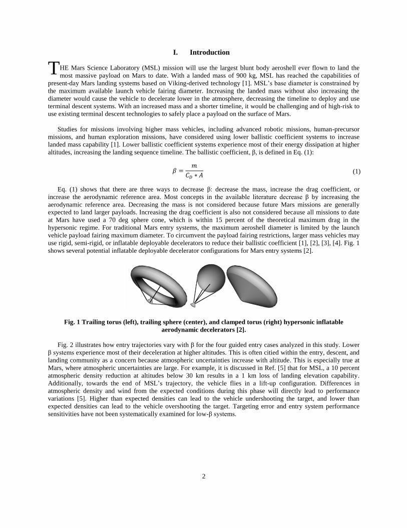
use rigid, semi-rigid, or inflatable deployable decelerators to reduce their ballistic coefficient [1], [2], [3], [4]. Fig. 1
shows several potential inflatable deployable decelerator configurations for Mars entry systems [2].
Fig. 1 Trailing torus (left), trailing sphere (center), and clamped torus (right) hypersonic inflatable
aerodynamic decelerators [2].
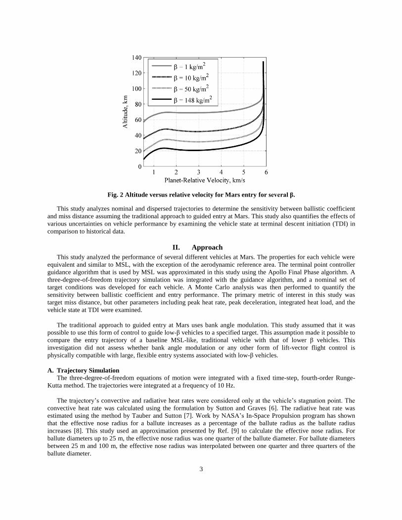
Fig. 2 illustrates how entry trajectories vary with β for the four guided entry cases analyzed in this study. Lower
β systems experience most of their deceleration at higher altitudes. This is often citied within the entry, descent, and
landing community as a concern because atmospheric uncertainties increase with altitude. This is especially true at
Mars, where atmospheric uncertainties are large. For example, it is discussed in Ref. [5] that for MSL, a 10 percent
atmospheric density reduction at altitudes below 30 km results in a 1 km loss of landing elevation capability.
Additionally, towards the end of MSL’s trajectory, the vehicle flies in a lift-up configuration. Differences in
atmospheric density and wind from the expected conditions during this phase will directly lead to performance
variations [5]. Higher than expected densities can lead to the vehicle undershooting the target, and lower than
expected densities can lead to the vehicle overshooting the target. Targeting error and entry system performance
sensitivities have not been systematically examined for low-β systems.
T
3
Fig. 2 Altitude versus relative velocity for Mars entry for several β.
This study analyzes nominal and dispersed trajectories to determine the sensitivity between ballistic coefficient
and miss distance assuming the traditional approach to guided entry at Mars. This study also quantifies the effects of
various uncertainties on vehicle performance by examining the vehicle state at terminal descent initiation (TDI) in
comparison to historical data.
II. Approach
This study analyzed the performance of several different vehicles at Mars. The properties for each vehicle were
equivalent and similar to MSL, with the exception of the aerodynamic reference area. The terminal point controller
guidance algorithm that is used by MSL was approximated in this study using the Apollo Final Phase algorithm. A
three-degree-of-freedom trajectory simulation was integrated with the guidance algorithm, and a nominal set of
target conditions was developed for each vehicle. A Monte Carlo analysis was then performed to quantify the
sensitivity between ballistic coefficient and entry performance. The primary metric of interest in this study was
target miss distance, but other parameters including peak heat rate, peak deceleration, integrated heat load, and the
vehicle state at TDI were examined.
The traditional approach to guided entry at Mars uses bank angle modulation. This study assumed that it was
possible to use this form of control to guide low-β vehicles to a specified target. This assumption made it possible to
compare the entry trajectory of a baseline MSL-like, traditional vehicle with that of lower β vehicles. This
investigation did not assess whether bank angle modulation or any other form of lift-vector flight control is
physically compatible with large, flexible entry systems associated with low-β vehicles.
A. Trajectory Simulation
The three-degree-of-freedom equations of motion were integrated with a fixed time-step, fourth-order Runge-
Kutta method. The trajectories were integrated at a frequency of 10 Hz.
The trajectory’s convective and radiative heat rates were considered only at the vehicle’s stagnation point. The
convective heat rate was calculated using the formulation by Sutton and Graves [6]. The radiative heat rate was
estimated using the method by Tauber and Sutton [7]. Work by NASA’s In-Space Propulsion program has shown
that the effective nose radius for a ballute increases as a percentage of the ballute radius as the ballute radius
increases [8]. This study used an approximation presented by Ref. [9] to calculate the effective nose radius. For
ballute diameters up to 25 m, the effective nose radius was one quarter of the ballute diameter. For ballute diameters
between 25 m and 100 m, the effective nose radius was interpolated between one quarter and three quarters of the
ballute diameter.
4
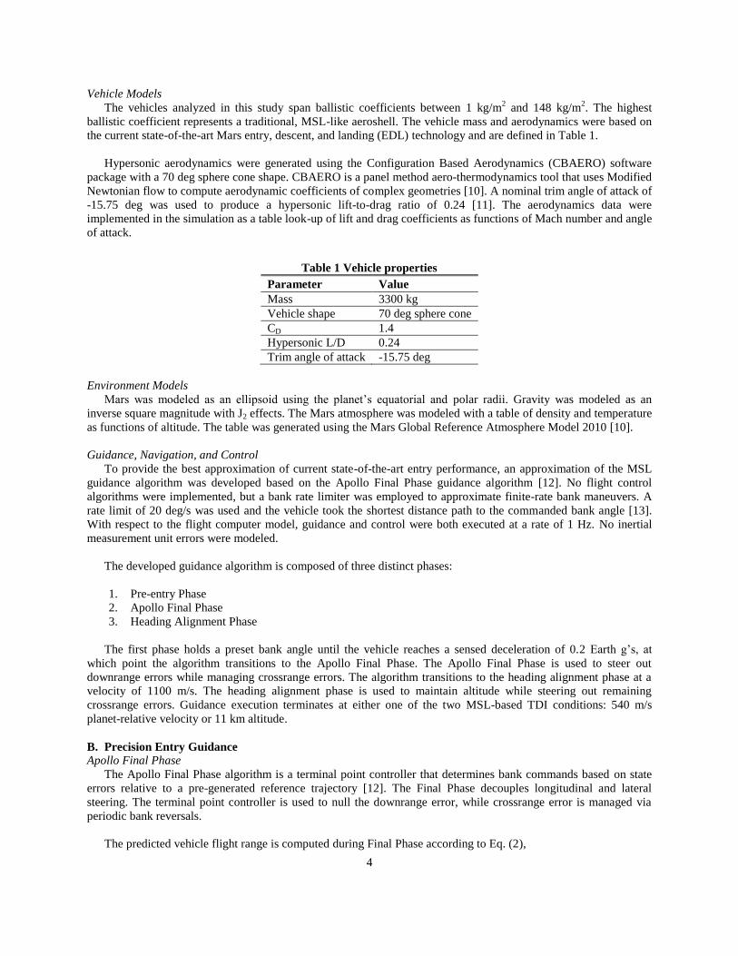
Vehicle Models
The vehicles analyzed in this study span ballistic coefficients between 1 kg/m2 and 148 kg/m
2. The highest
ballistic coefficient represents a traditional, MSL-like aeroshell. The vehicle mass and aerodynamics were based on
the current state-of-the-art Mars entry, descent, and landing (EDL) technology and are defined in Table 1.
Hypersonic aerodynamics were generated using the Configuration Based Aerodynamics (CBAERO) software
package with a 70 deg sphere cone shape. CBAERO is a panel method aero-thermodynamics tool that uses Modified
Newtonian flow to compute aerodynamic coefficients of complex geometries [10]. A nominal trim angle of attack of
-15.75 deg was used to produce a hypersonic lift-to-drag ratio of 0.24 [11]. The aerodynamics data were
implemented in the simulation as a table look-up of lift and drag coefficients as functions of Mach number and angle
of attack.
Table 1 Vehicle properties
Parameter Value
Mass 3300 kg
Vehicle shape 70 deg sphere cone
CD 1.4
Hypersonic L/D 0.24
Trim angle of attack -15.75 deg
Environment Models
Mars was modeled as an ellipsoid using the planet’s equatorial and polar radii. Gravity was modeled as an
inverse square magnitude with J2 effects. The Mars atmosphere was modeled with a table of density and temperature
as functions of altitude. The table was generated using the Mars Global Reference Atmosphere Model 2010 [10].
Guidance, Navigation, and Control
To provide the best approximation of current state-of-the-art entry performance, an approximation of the MSL
guidance algorithm was developed based on the Apollo Final Phase guidance algorithm [12]. No flight control
algorithms were implemented, but a bank rate limiter was employed to approximate finite-rate bank maneuvers. A
rate limit of 20 deg/s was used and the vehicle took the shortest distance path to the commanded bank angle [13].
With respect to the flight computer model, guidance and control were both executed at a rate of 1 Hz. No inertial
measurement unit errors were modeled.
The developed guidance algorithm is composed of three distinct phases:
1. Pre-entry Phase
2. Apollo Final Phase
3. Heading Alignment Phase
The first phase holds a preset bank angle until the vehicle reaches a sensed deceleration of 0.2 Earth g’s, at
which point the algorithm transitions to the Apollo Final Phase. The Apollo Final Phase is used to steer out
downrange errors while managing crossrange errors. The algorithm transitions to the heading alignment phase at a
velocity of 1100 m/s. The heading alignment phase is used to maintain altitude while steering out remaining
crossrange errors. Guidance execution terminates at either one of the two MSL-based TDI conditions: 540 m/s
planet-relative velocity or 11 km altitude.
B. Precision Entry Guidance
Apollo Final Phase
The Apollo Final Phase algorithm is a terminal point controller that determines bank commands based on state
errors relative to a pre-generated reference trajectory [12]. The Final Phase decouples longitudinal and lateral
steering. The terminal point controller is used to null the downrange error, while crossrange error is managed via
periodic bank reversals.
The predicted vehicle flight range is computed during Final Phase according to Eq. (2),
5
( ) ( ) ( ( )) ( ) ( ( )) (2)
where is the reference trajectory’s range, is the altitude rate, D is the vehicle’s drag, V is the vehicle’s
velocity, and and are the partial derivatives of range with respect to drag acceleration and altitude rate,
respectively. Reference values for the drag acceleration, Dref, and altitude rate, , are stored in the reference
trajectory as functions of velocity.
The L/D commands are generated with Eq. (3),
(
)
(
) ( )
(3)
where (L/D)cmd is the commanded vertical lift-to-drag ratio, (L/D)ref is the constant reference trajectory vertical L/D
command, rtogo is the range to the target, xtogo is the predicted vehicle flight range during the Final Phase, and F3 is
the partial derivative of range with respect to vertical L/D and is stored in a table.
The lateral channel periodically commands bank reversals to manage crossrange error during entry. Guidance
computes the estimated crossrange error each cycle and determines the crossrange error limit as a function of
velocity. If the crossrange error exceeds the limit, a bank reversal is commanded. The crossrange error limit is given
by Eq. (4),
(
)
(4)
where Klateral and Kbias are gains, raverage is the average radius of the planet, and Vcircular is the circular orbital velocity
at the planet’s surface. The limit, Y, is computed in radians. This crossrange limit decreases with the square of the
velocity to ensure that the allowable errors decrease with decreasing control authority. For velocities above 3 km/s,
the corridor width is divided by four to force an early bank reversal in most trajectories.
The bank command is calculated from Eq. (5),
(
( )⁄
( )⁄
) (5)
where is the bank command and (L/D)nom is the vehicle’s nominal lift-to-drag ratio. The ± sign is determined
by the lateral channel.
Heading Alignment Phase
The heading alignment phase begins at a velocity of 1100 m/s. The heading alignment phase’s goals are to null
the crossrange error and maintain altitude for TDI. Downrange errors are completely neglected during this phase,
highlighting the importance of altitude maintenance over accuracy for Mars missions to date. Bank commands
during this phase are generated from Eq. (6),
(
) (6)
where K is a proportional gain, λ is the current heading angle error, and θ is the current angular range to target. A
gain value of 100 was found to provide a good balance between accuracy and bank command stability. Bank
commands are limited between ± 30 deg to maintain altitude.
Final Phase Reference Trajectory Design
New reference trajectories were generated for each vehicle concept in this study. This process was modified
from the original formulation that is described in Ref. [12] to include Mach-dependent vehicle aerodynamics and

6
bank profile. Initial conditions for the reference trajectory were selected to match the expected vehicle state at the
start of the Apollo Final Phase. The reference bank profile was chosen to provide the best overall accuracy at the
terminal state.
The reference trajectory was generated by first integrating simplified entry equations of motion from a given
initial state to the desired TDI state using an assumed reference bank command profile. The simplified equations of
motion assumed a non-rotating spherical planet. Then, the adjoint equations were integrated backwards in time from
TDI to generate the reference control gains. The data, including the reference commands, were then compiled into a
single table as a function of velocity for use in the guidance algorithm.
The type of bank angle profile developed in Ref. [11] was used for this study. The profile is a linear function
with constant tails that are defined by the early and late bank angles. Fig. 3 shows the reference command as a
function of velocity for the baseline vehicle in this study. The constant early bank angle is used for velocities above
6 km/s. Between 2.5 km/s and 6 km/s, the reference bank command is linearly interpolated between the early bank
angle and late bank angle. Between 1.1 km/s and 2.5 km/s, the constant late bank angle is used. Velocities below 1.1
km/s, the heading alignment starting velocity, use a reference bank angle of 21.1 deg. This section of the bank
profile is used to account for the heading alignment phase in which the bank angle varies between ± 30 deg. A bank
angle of 21.1 deg corresponds to one half of the vertical lift between 0 deg and 30 deg. All trajectories in this study
used the bank angle profile shown in Fig. 3. This type of bank angle profile is well-suited to Mars entry: the vehicle
dives into the thicker atmosphere early in the trajectory and then slowly transitions to a more lift-up orientation to
maintain altitude at parachute deploy.
Fig. 3 Reference bank profile for the baseline vehicle.
C. Mission Design
The entry interface state is the initial state of the trajectory simulation. The entry velocity and altitude in this
study were selected to be consistent with the MSL entry state [11]. All ballistic coefficient systems in this study used
the same entry interface state, with the exception of the entry flight-path angle. This parameter was selected so that
the peak deceleration for each system matched that of the baseline case. Two different trajectory termination
conditions were considered: a planet-relative velocity of 540 m/s and an altitude of 11 km. These conditions
correspond to the approximate parachute deploy conditions of MSL [11]. Vehicles whose ballistic coefficients differ
from MSL fly different entry trajectories and because of this, these parachute deploy conditions do not occur
simultaneously. To accommodate this, the vehicle states at each of the MSL parachute deploy conditions were
analyzed independently. The terminal descent sequence was not considered in this study, so the vehicle state at the
terminal condition is referred to as the “terminal descent initiation” (TDI) state.
7
D. Monte Carlo Design Uncertainties
Monte Carlo simulations were computed to analyze the performance sensitivity of the lower ballistic coefficient
systems when subjected to day-of-flight uncertainties. Probability distributions were assigned to relevant simulation
model parameters, including vehicle aerodynamics, atmospheric parameters, vehicle mass, and initial vehicle state.
Table 2 shows the nominal value, distribution type, and distribution parameters for each dispersed parameter. These
parameters were based on past Mars uncertainty analyses [12]. The distributions were used to generate 1000
dispersed sets of inputs and model parameters. To provide more conservative results, the entry state uncertainties
were not correlated.
Table 2 Monte Carlo dispersions
Parameter Nominal Distribution Deviation, 3σ or
min/max
Entry mass, kg [12] 3300 Gaussian 3.0 kg
Axial-force coefficient multiplier, nd [12] 1.0 Gaussian 3 %
Normal-force coefficient multiplier, nd [12] 1.0 Gaussian 5 %
Trim angle of attack, deg [12] -15.75 Gaussian 2.0
Inertial entry flight-path angle, deg -15.5, -14.7, -14.3, -11.7 * Gaussian 0.050 deg
Entry latitude, deg 0 Gaussian 0.100 deg
Entry longitude, deg 0 Gaussian 0.100 deg
Entry azimuth, deg 90 Gaussian 0.005 deg
Inertial entry velocity magnitude, m/s 6100 Gaussian 2.0 m/s
Entry altitude, km 135 Gaussian 2.5 km
Atmosphere dust opacity (Dust Tau), nd 0.45 Uniform 0.1 / 0.9
* Listed for β = 148 kg/m2, 50 kg/m
2, 10 kg/m
2, and 1 kg/m
2, respectively
Mars-GRAM was used to generate a set of 1000 dispersed atmospheres with which the different ballistic
coefficient systems were tested. These atmospheres included dispersions in atmospheric winds and density. The
nominal atmosphere was generated by calculating the mean of the set of dispersed atmospheres.
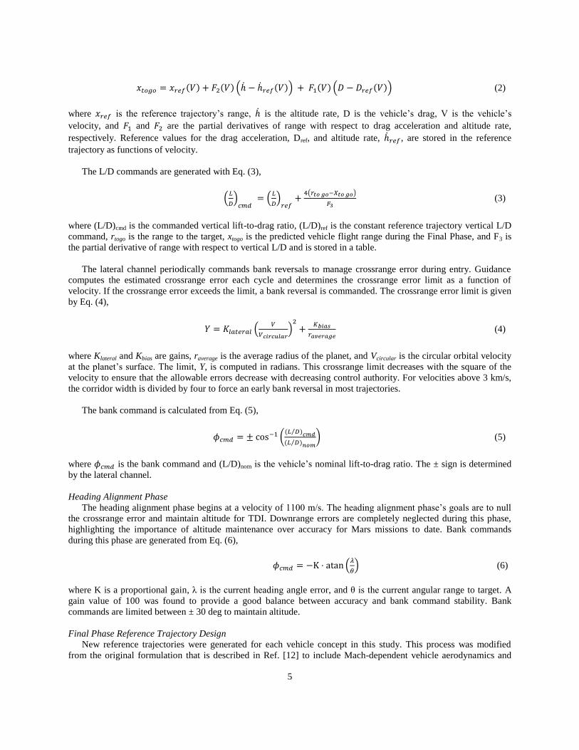
Fig. 4 shows a plot of the nominal density variation with altitude used in the Monte Carlo simulations. Near the
entry altitude of 135 km, the 3-σ dispersed density was 107 percent of the nominal density. At altitudes below 20
km, the density was much less dispersed, with a 3-σ variation of approximately 9 percent of the nominal density.
Fig. 4 Mars-GRAM density variations.
8
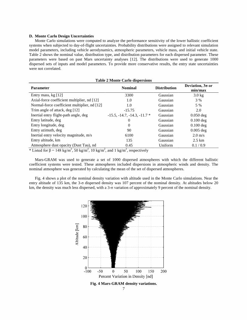
Fig. 5 shows the variation in wind magnitude as a function of altitude used in the Monte Carlo simulations. Wind
variations are largest between altitudes of 0 km to 20 km and 80 km to 110 km.
Fig. 5 Mars-GRAM wind variations.
E. Performance Metrics
Several metrics were used to assess the performance of the different ballistic coefficient systems in this study.
These metrics included the TDI vehicle state, peak sensed deceleration, peak heat rate, and integrated heat load.
Target miss distance, altitude, dynamic pressure, and Mach number were all considered at TDI. Miss distance was
calculated using Vincenty’s method [14] by comparing the latitude and longitude at TDI with the target latitude and
longitude. The iterative method developed by Vincenty computes the distance between two points by assuming that
the planet is an oblate spheroid. The peak heat rate was the maximum sum of the convective heat rate and the
radiative heat rate.
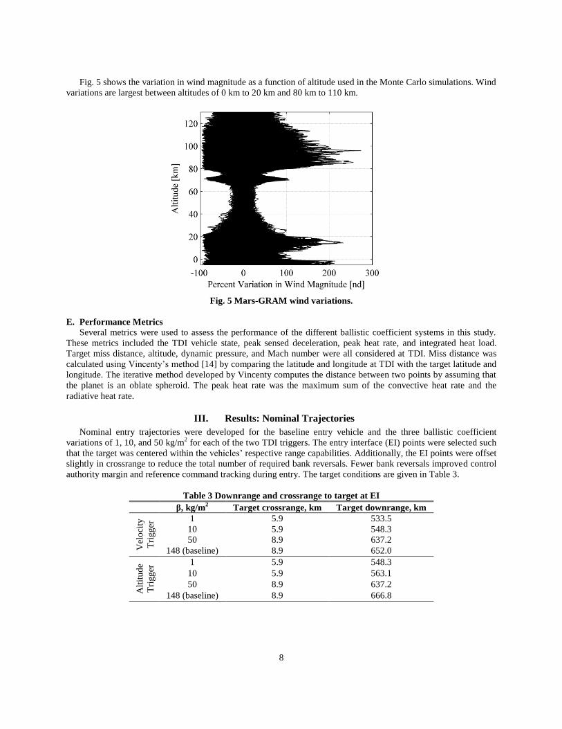
III. Results: Nominal Trajectories
Nominal entry trajectories were developed for the baseline entry vehicle and the three ballistic coefficient
variations of 1, 10, and 50 kg/m2 for each of the two TDI triggers. The entry interface (EI) points were selected such
that the target was centered within the vehicles’ respective range capabilities. Additionally, the EI points were offset
slightly in crossrange to reduce the total number of required bank reversals. Fewer bank reversals improved control
authority margin and reference command tracking during entry. The target conditions are given in Table 3.
Table 3 Downrange and crossrange to target at EI
β, kg/m2 Target crossrange, km Target downrange, km
Vel
oci
ty
Tri
gg
er 1 5.9 533.5
10 5.9 548.3
50 8.9 637.2
148 (baseline) 8.9 652.0
Alt
itu
de
Tri
gg
er 1 5.9 548.3
10 5.9 563.1
50 8.9 637.2
148 (baseline) 8.9 666.8
9
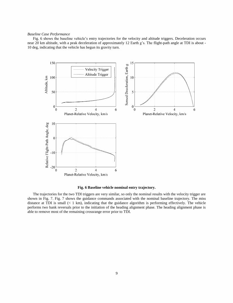
Baseline Case Performance
Fig. 6 shows the baseline vehicle’s entry trajectories for the velocity and altitude triggers. Deceleration occurs
near 20 km altitude, with a peak deceleration of approximately 12 Earth g’s. The flight-path angle at TDI is about -
10 deg, indicating that the vehicle has begun its gravity turn.
Fig. 6 Baseline vehicle nominal entry trajectory.
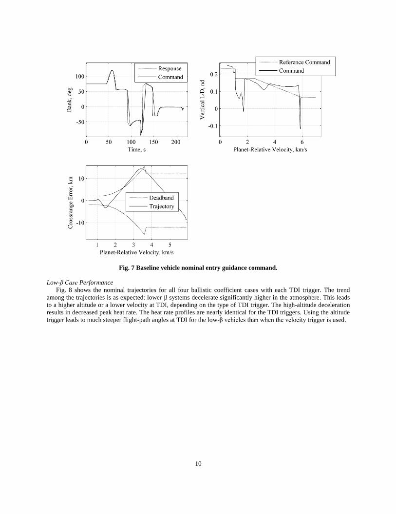
The trajectories for the two TDI triggers are very similar, so only the nominal results with the velocity trigger are
shown in Fig. 7. Fig. 7 shows the guidance commands associated with the nominal baseline trajectory. The miss
distance at TDI is small (< 1 km), indicating that the guidance algorithm is performing effectively. The vehicle
performs two bank reversals prior to the initiation of the heading alignment phase. The heading alignment phase is
able to remove most of the remaining crossrange error prior to TDI.
10
Fig. 7 Baseline vehicle nominal entry guidance command.
Low-β Case Performance
Fig. 8 shows the nominal trajectories for all four ballistic coefficient cases with each TDI trigger. The trend
among the trajectories is as expected: lower β systems decelerate significantly higher in the atmosphere. This leads
to a higher altitude or a lower velocity at TDI, depending on the type of TDI trigger. The high-altitude deceleration
results in decreased peak heat rate. The heat rate profiles are nearly identical for the TDI triggers. Using the altitude
trigger leads to much steeper flight-path angles at TDI for the low-β vehicles than when the velocity trigger is used.

11
a) Velocity Trigger b) Altitude Trigger
c) Velocity Trigger d) Altitude Trigger
e) Velocity Trigger f) Altitude Trigger
Fig. 8 Nominal trajectories for several ballistic coefficients for a)/b) altitude, c)/d) peak heat rate, and e)/f)
relative flight-path angle.
12
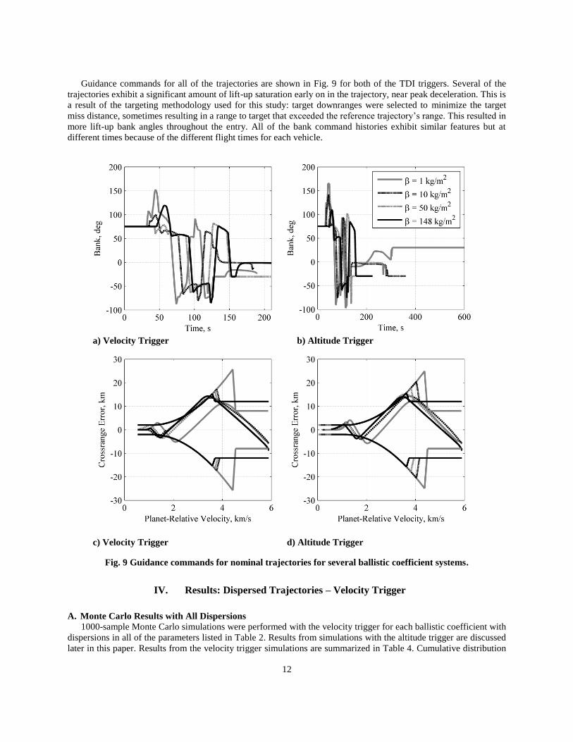
Guidance commands for all of the trajectories are shown in Fig. 9 for both of the TDI triggers. Several of the
trajectories exhibit a significant amount of lift-up saturation early on in the trajectory, near peak deceleration. This is
a result of the targeting methodology used for this study: target downranges were selected to minimize the target
miss distance, sometimes resulting in a range to target that exceeded the reference trajectory’s range. This resulted in
more lift-up bank angles throughout the entry. All of the bank command histories exhibit similar features but at
different times because of the different flight times for each vehicle.
a) Velocity Trigger b) Altitude Trigger
c) Velocity Trigger d) Altitude Trigger
Fig. 9 Guidance commands for nominal trajectories for several ballistic coefficient systems.
IV. Results: Dispersed Trajectories – Velocity Trigger
A. Monte Carlo Results with All Dispersions
1000-sample Monte Carlo simulations were performed with the velocity trigger for each ballistic coefficient with
dispersions in all of the parameters listed in Table 2. Results from simulations with the altitude trigger are discussed
later in this paper. Results from the velocity trigger simulations are summarized in Table 4. Cumulative distribution
13
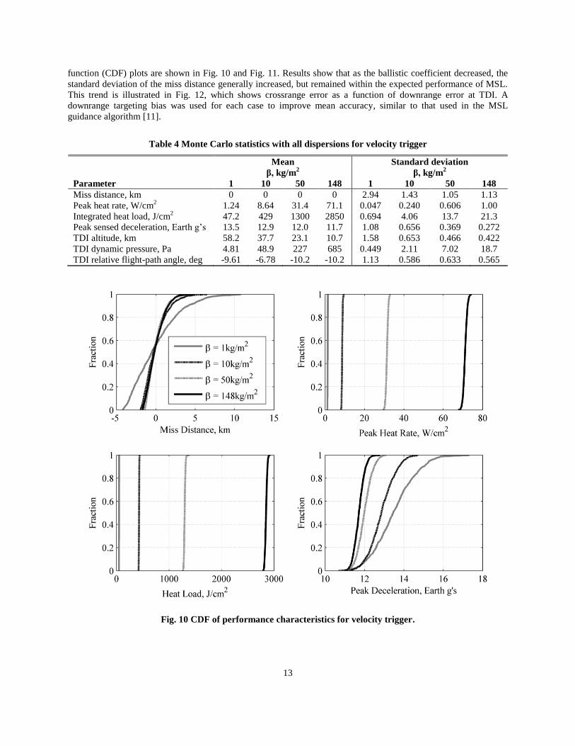
function (CDF) plots are shown in Fig. 10 and Fig. 11. Results show that as the ballistic coefficient decreased, the
standard deviation of the miss distance generally increased, but remained within the expected performance of MSL.
This trend is illustrated in Fig. 12, which shows crossrange error as a function of downrange error at TDI. A
downrange targeting bias was used for each case to improve mean accuracy, similar to that used in the MSL
guidance algorithm [11].
Table 4 Monte Carlo statistics with all dispersions for velocity trigger
Mean Standard deviation
β, kg/m2 β, kg/m
2
Parameter 1 10 50 148 1 10 50 148
Miss distance, km 0 0 0 0 2.94 1.43 1.05 1.13
Peak heat rate, W/cm2 1.24 8.64 31.4 71.1 0.047 0.240 0.606 1.00
Integrated heat load, J/cm2 47.2 429 1300 2850 0.694 4.06 13.7 21.3
Peak sensed deceleration, Earth g’s 13.5 12.9 12.0 11.7 1.08 0.656 0.369 0.272
TDI altitude, km 58.2 37.7 23.1 10.7 1.58 0.653 0.466 0.422
TDI dynamic pressure, Pa 4.81 48.9 227 685 0.449 2.11 7.02 18.7
TDI relative flight-path angle, deg -9.61 -6.78 -10.2 -10.2 1.13 0.586 0.633 0.565
Fig. 10 CDF of performance characteristics for velocity trigger.

14
Fig. 11 CDF of TDI conditions for velocity trigger.
15
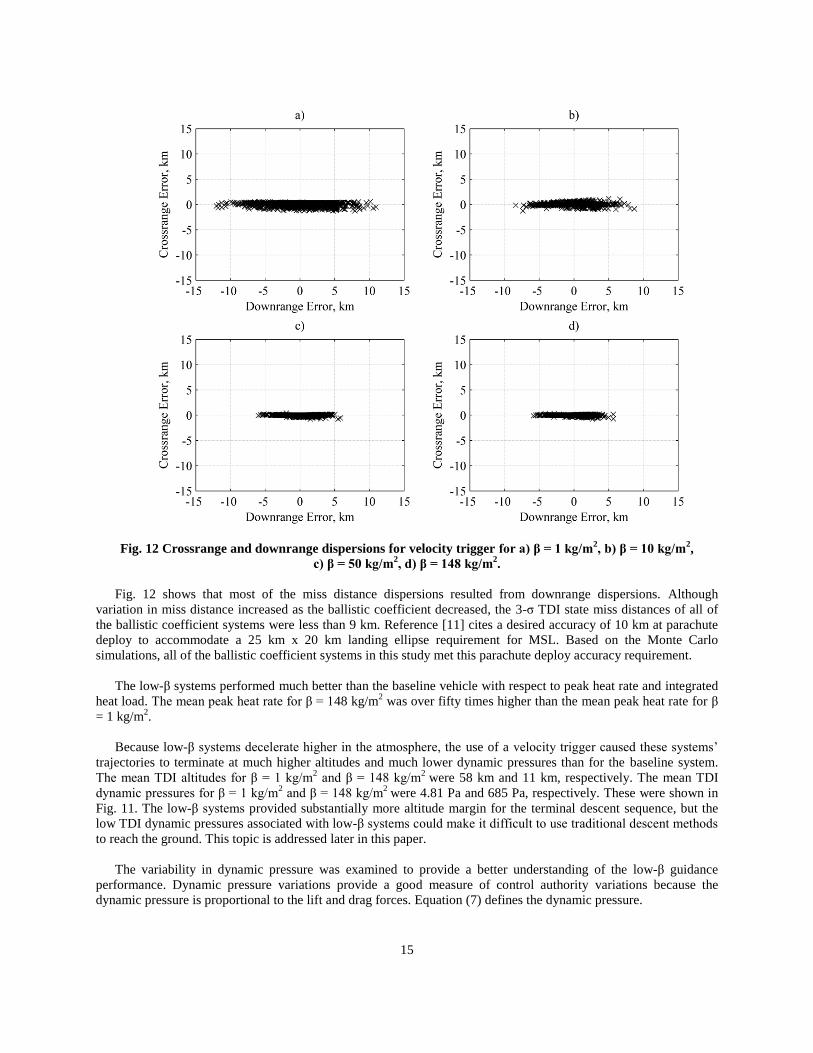
Fig. 12 Crossrange and downrange dispersions for velocity trigger for a) β = 1 kg/m
2, b) β = 10 kg/m
2,
c) β = 50 kg/m2, d) β = 148 kg/m
2.
Fig. 12 shows that most of the miss distance dispersions resulted from downrange dispersions. Although
variation in miss distance increased as the ballistic coefficient decreased, the 3-σ TDI state miss distances of all of
the ballistic coefficient systems were less than 9 km. Reference [11] cites a desired accuracy of 10 km at parachute
deploy to accommodate a 25 km x 20 km landing ellipse requirement for MSL. Based on the Monte Carlo
simulations, all of the ballistic coefficient systems in this study met this parachute deploy accuracy requirement.
The low-β systems performed much better than the baseline vehicle with respect to peak heat rate and integrated
heat load. The mean peak heat rate for β = 148 kg/m2 was over fifty times higher than the mean peak heat rate for β
= 1 kg/m2.
Because low-β systems decelerate higher in the atmosphere, the use of a velocity trigger caused these systems’
trajectories to terminate at much higher altitudes and much lower dynamic pressures than for the baseline system.
The mean TDI altitudes for β = 1 kg/m2 and β = 148 kg/m
2 were 58 km and 11 km, respectively. The mean TDI
dynamic pressures for β = 1 kg/m2 and β = 148 kg/m
2 were 4.81 Pa and 685 Pa, respectively. These were shown in
Fig. 11. The low-β systems provided substantially more altitude margin for the terminal descent sequence, but the
low TDI dynamic pressures associated with low-β systems could make it difficult to use traditional descent methods
to reach the ground. This topic is addressed later in this paper.
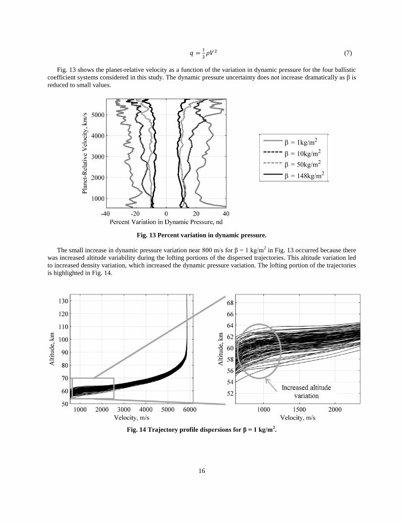
The variability in dynamic pressure was examined to provide a better understanding of the low-β guidance
performance. Dynamic pressure variations provide a good measure of control authority variations because the
dynamic pressure is proportional to the lift and drag forces. Equation (7) defines the dynamic pressure.
16
(7)
Fig. 13 shows the planet-relative velocity as a function of the variation in dynamic pressure for the four ballistic
coefficient systems considered in this study. The dynamic pressure uncertainty does not increase dramatically as β is
reduced to small values.
Fig. 13 Percent variation in dynamic pressure.
The small increase in dynamic pressure variation near 800 m/s for β = 1 kg/m2 in Fig. 13 occurred because there
was increased altitude variability during the lofting portions of the dispersed trajectories. This altitude variation led
to increased density variation, which increased the dynamic pressure variation. The lofting portion of the trajectories
is highlighted in Fig. 14.
Fig. 14 Trajectory profile dispersions for β = 1 kg/m2.
0 100 200 300 400 500 6000
1000
2000
3000
4000
5000
6000
7000
= 1kg/m2
= 10kg/m2
= 50kg/m2
= 148kg/m2
17
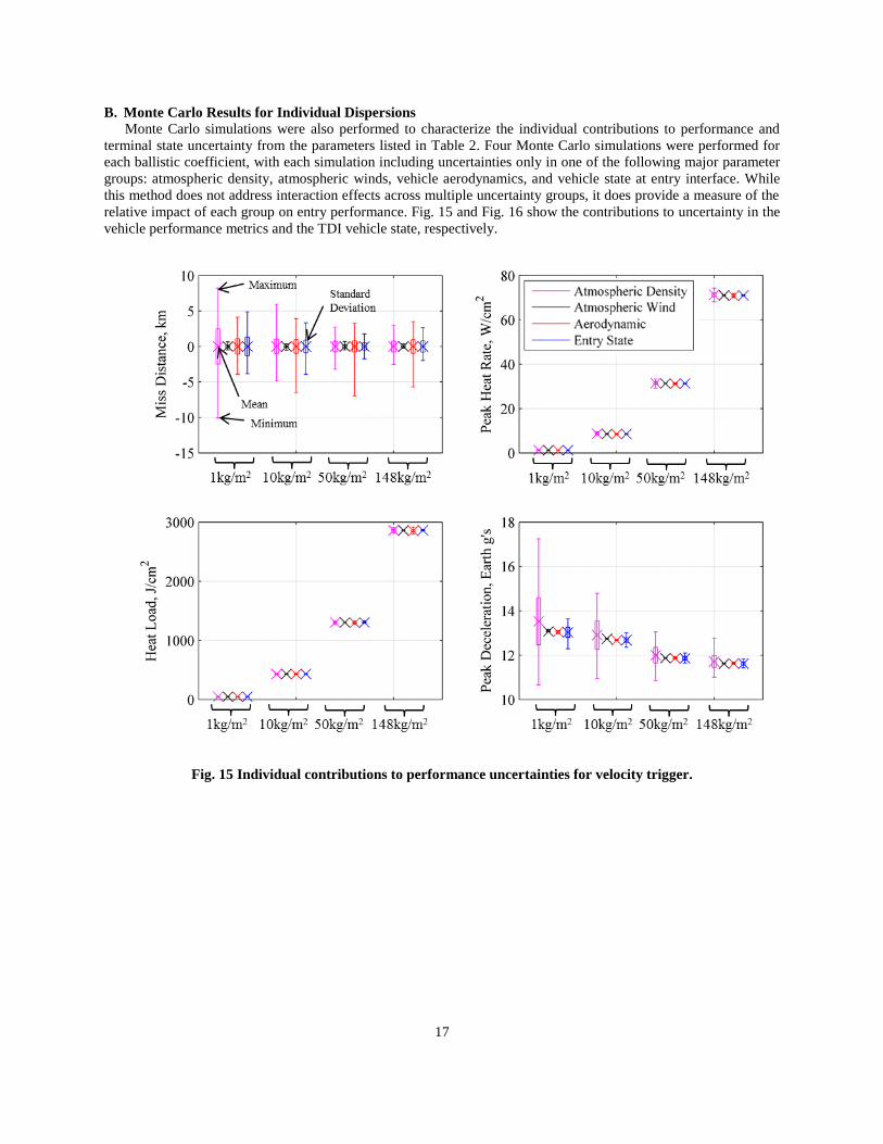
B. Monte Carlo Results for Individual Dispersions
Monte Carlo simulations were also performed to characterize the individual contributions to performance and
terminal state uncertainty from the parameters listed in Table 2. Four Monte Carlo simulations were performed for
each ballistic coefficient, with each simulation including uncertainties only in one of the following major parameter
groups: atmospheric density, atmospheric winds, vehicle aerodynamics, and vehicle state at entry interface. While
this method does not address interaction effects across multiple uncertainty groups, it does provide a measure of the
relative impact of each group on entry performance. Fig. 15 and Fig. 16 show the contributions to uncertainty in the
vehicle performance metrics and the TDI vehicle state, respectively.
Fig. 15 Individual contributions to performance uncertainties for velocity trigger.

18
Fig. 16 Individual contributions to terminal state uncertainties for velocity trigger.
Fig. 15 shows that for β higher than 1 kg/m2, the standard deviations of the contributions to miss distance from
each of the parameters were relatively equal, with the exception of the atmospheric wind uncertainties. Wind
uncertainty standard deviations were small for all β systems. Atmospheric density uncertainty was the largest
contributor to miss distance variability for β = 1 kg/m2 with respect to standard deviation. Lower β systems
experience most of their decelerations at higher altitudes, and density uncertainties are higher at these altitudes. This
behavior is overlaid with density uncertainty and wind uncertainty in Fig. 17 and Fig. 18, respectively. Although
Fig. 18 shows that standard deviations due to wind uncertainties are greater at lower altitudes (where high-β vehicles
decelerate), the contributions from wind uncertainties were small for all β systems.

19
Fig. 17 Primary altitudes of deceleration for various ballistic coefficient systems overlaid with density
uncertainty.
Fig. 18 Primary altitudes of deceleration for various ballistic coefficient systems overlaid with wind
uncertainty.
V. Results: Dispersed Trajectories – Altitude Trigger
A. Monte Carlo Results with All Dispersions
1000-sample Monte Carlo simulations were also performed for each ballistic coefficient when the trajectories
were terminated with an altitude trigger. The same dispersions that were used for the velocity trigger were used for
the altitude trigger. The mean and standard deviation in the miss distance are provided in Table 5. Results show that
as the ballistic coefficient decreased, the standard deviation of the miss distance increased. This trend is illustrated in
Fig. 19. This trend was also observed when the velocity trigger was used for TDI.
Table 5 Monte Carlo miss distance statistics with all dispersions for altitude trigger
Mean, km Standard deviation, km
β, kg/m2 β, kg/m
2
1 10 50 148 1 10 50 148
0 0 0 0 3.09 1.71 1.16 1.16
20
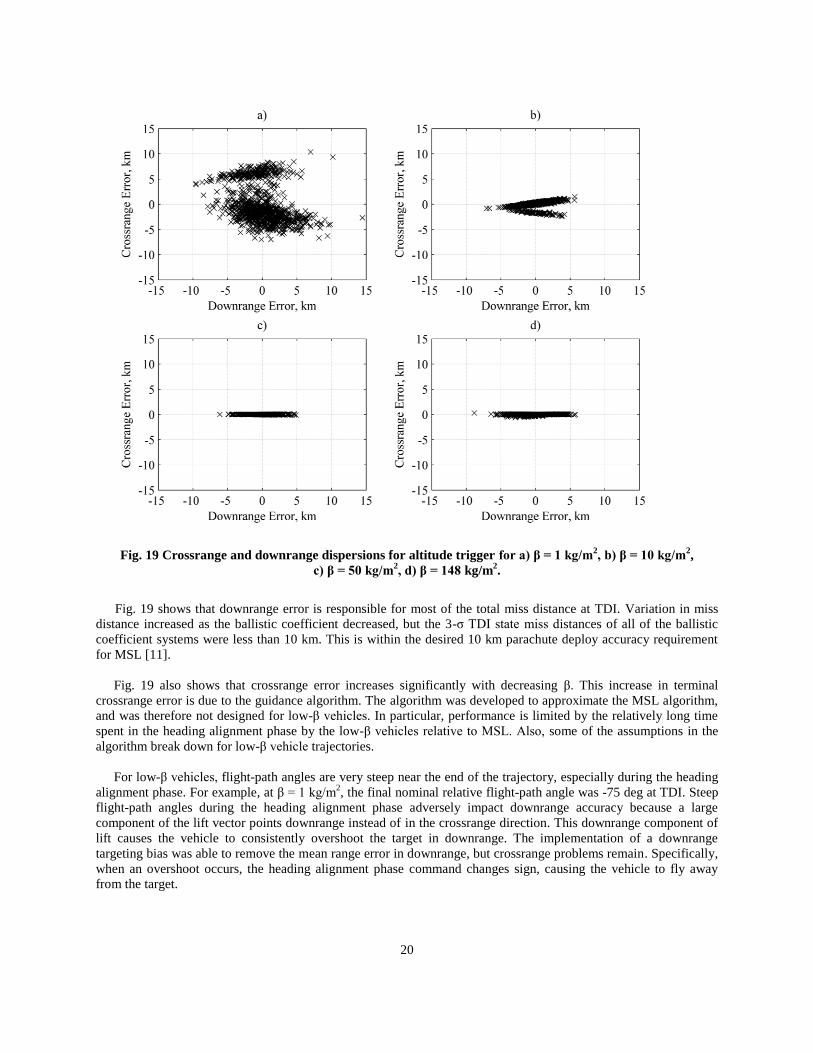
Fig. 19 Crossrange and downrange dispersions for altitude trigger for a) β = 1 kg/m2, b) β = 10 kg/m
2,
c) β = 50 kg/m2, d) β = 148 kg/m
2.
Fig. 19 shows that downrange error is responsible for most of the total miss distance at TDI. Variation in miss
distance increased as the ballistic coefficient decreased, but the 3-σ TDI state miss distances of all of the ballistic
coefficient systems were less than 10 km. This is within the desired 10 km parachute deploy accuracy requirement
for MSL [11].
Fig. 19 also shows that crossrange error increases significantly with decreasing β. This increase in terminal
crossrange error is due to the guidance algorithm. The algorithm was developed to approximate the MSL algorithm,
and was therefore not designed for low-β vehicles. In particular, performance is limited by the relatively long time
spent in the heading alignment phase by the low-β vehicles relative to MSL. Also, some of the assumptions in the
algorithm break down for low-β vehicle trajectories.
For low-β vehicles, flight-path angles are very steep near the end of the trajectory, especially during the heading
alignment phase. For example, at β = 1 kg/m2, the final nominal relative flight-path angle was -75 deg at TDI. Steep
flight-path angles during the heading alignment phase adversely impact downrange accuracy because a large
component of the lift vector points downrange instead of in the crossrange direction. This downrange component of
lift causes the vehicle to consistently overshoot the target in downrange. The implementation of a downrange
targeting bias was able to remove the mean range error in downrange, but crossrange problems remain. Specifically,
when an overshoot occurs, the heading alignment phase command changes sign, causing the vehicle to fly away
from the target.
21
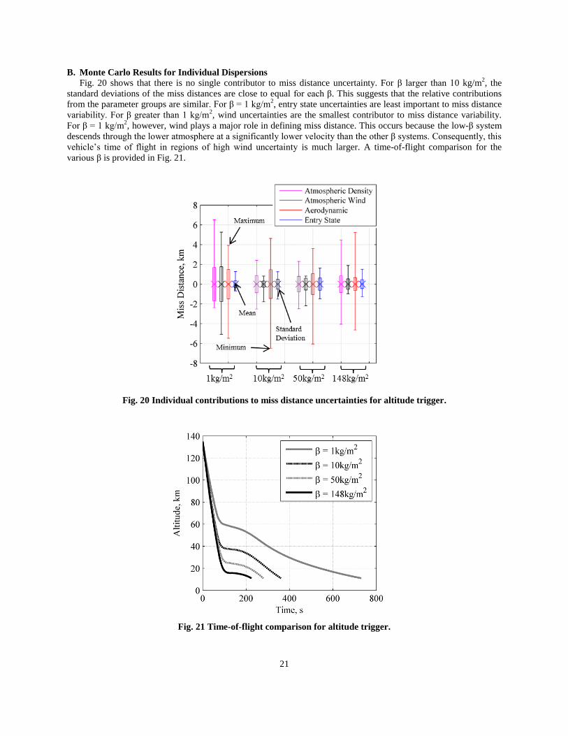
B. Monte Carlo Results for Individual Dispersions
Fig. 20 shows that there is no single contributor to miss distance uncertainty. For β larger than 10 kg/m2, the
standard deviations of the miss distances are close to equal for each β. This suggests that the relative contributions
from the parameter groups are similar. For β = 1 kg/m2, entry state uncertainties are least important to miss distance
variability. For β greater than 1 kg/m2, wind uncertainties are the smallest contributor to miss distance variability.
For β = 1 kg/m2, however, wind plays a major role in defining miss distance. This occurs because the low-β system
descends through the lower atmosphere at a significantly lower velocity than the other β systems. Consequently, this
vehicle’s time of flight in regions of high wind uncertainty is much larger. A time-of-flight comparison for the
various β is provided in Fig. 21.
Fig. 20 Individual contributions to miss distance uncertainties for altitude trigger.
Fig. 21 Time-of-flight comparison for altitude trigger.
22
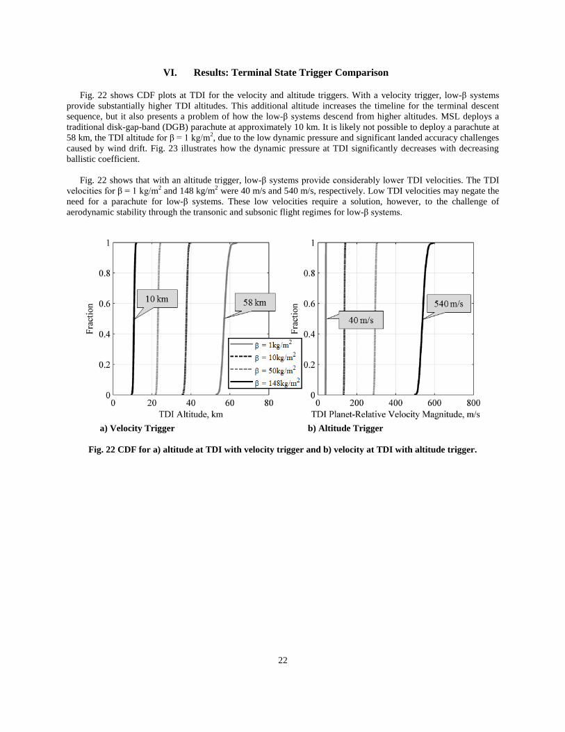
VI. Results: Terminal State Trigger Comparison
Fig. 22 shows CDF plots at TDI for the velocity and altitude triggers. With a velocity trigger, low-β systems
provide substantially higher TDI altitudes. This additional altitude increases the timeline for the terminal descent
sequence, but it also presents a problem of how the low-β systems descend from higher altitudes. MSL deploys a
traditional disk-gap-band (DGB) parachute at approximately 10 km. It is likely not possible to deploy a parachute at
58 km, the TDI altitude for β = 1 kg/m2, due to the low dynamic pressure and significant landed accuracy challenges
caused by wind drift. Fig. 23 illustrates how the dynamic pressure at TDI significantly decreases with decreasing
ballistic coefficient.
Fig. 22 shows that with an altitude trigger, low-β systems provide considerably lower TDI velocities. The TDI
velocities for β = 1 kg/m2 and 148 kg/m
2 were 40 m/s and 540 m/s, respectively. Low TDI velocities may negate the
need for a parachute for low-β systems. These low velocities require a solution, however, to the challenge of
aerodynamic stability through the transonic and subsonic flight regimes for low-β systems.
a) Velocity Trigger b) Altitude Trigger
Fig. 22 CDF for a) altitude at TDI with velocity trigger and b) velocity at TDI with altitude trigger.

23
a) Velocity Trigger b) Altitude Trigger
Fig. 23 CDF for dynamic pressure at TDI for a) velocity trigger and b) altitude trigger.
Fig. 24 shows a history of DGB parachute inflation in Mars-relevant conditions, including the TDI conditions for
the systems considered in this study. Traditional DGB parachutes have been qualified to deploy at a dynamic
pressure between 250 Pa and 700 Pa and a Mach number between 1.4 and 2.1 [1]. Fig. 24 shows that these
conditions are not met for β = 1 kg/m2 and 10 kg/m
2. If parachutes are to be used as complements to low-β systems
at Mars, Fig. 24 suggests that more work is needed to either re-qualify DGB parachutes at new deployment
conditions or to develop novel terminal descent systems. As discussed previously, low-β system architectures may
not employ a parachute and instead address the challenge of transonic and subsonic stability. Past work has studied
options for expanding the dynamic pressure and Mach number envelope to either higher [15] or lower conditions
[16].

24
Fig. 24 History of DGB parachute inflation in Mars-relevant conditions [1].
VII. Conclusions
This analysis presented the guided entry performance of low ballistic coefficient vehicles at Mars using an MSL-
like guidance algorithm. Entry performance metrics of interest, including target miss distance, were presented for
several ballistic coefficient systems. Prior to this study, it was hypothesized that atmospheric uncertainties would
have a detrimental effect on targeting accuracy for such vehicles. Results from this study verified this trend, but
showed that this effect is small in magnitude. A velocity and an altitude trigger were evaluated as a means to
terminate the guided entry phase. Use of these two triggers produced significant differences in entry performance
and termination conditions, but both are compatible with desired accuracy requirements. Results from this study
suggest that it is feasible, in terms of targeting requirements, to use guided entry vehicles at Mars with large
diameter aeroshells.
This analysis also compared the vehicle state at the end of the guided entry phase with traditional Mars entry
systems. Relative to traditional high ballistic coefficient systems at Mars, low ballistic coefficient systems provide
higher terminal state altitudes when a velocity trigger is used, and they provide lower terminal state velocities when
an altitude trigger is used. In each case, dynamic pressure is affected significantly, and the stability of low ballistic
coefficient vehicles in these flight regimes should be investigated. The increased crossrange error exhibited by low
ballistic coefficient trajectories when the altitude trigger was used suggests that guidance modifications should be
considered to improve the performance for the low-velocity, high flight-path angle trajectory phase. Work in these
areas would make it possible to take advantage of the benefits presented by low ballistic coefficient trajectories.
References
[1] Braun, R. D. and Manning, R. M., “Mars Exploration Entry, Descent and Landing Challenges”, Journal of Spacecraft and
Rockets, Vol. 44, No. 2, 2007, pp. 310-323.
[2] Clark, I. G., Braun, R. D., Theisinger, J.T., and Wells, G.W., “An Evaluation of Ballute Entry Systems for Lunar Missions,”
AIAA Paper 2006-6276, Aug. 2006.
[3] Dweyer Cianciolo, A., et al, “Entry, Descent and Landing Systems Analysis Study: Phase 1 Report,” NASA-TM-2010-
216720, July 2010.
25
[4] Adler, M. et al, “Draft Entry, Descent, and Landing Roadmap: Technology Area 09,” NASA, November 2010.
[5] Chen, A. et al., “Atmospheric Risk Assessment for the Mars Science Laboratory Entry, Descent, and Landing System,”
IEEEAC Paper 1153, March 2010.
[6] Sutton, K. S., and Graves, Jr., R. A., “A General Stagnation-Point Convective-Heating Equation for Arbitrary Gas
Mixtures,” NASA TR-R-376, Nov. 1971.
[7] Tauber, M. E., and Sutton, K., “Stagnation-Point Radiative Heating Relations for Earth and Mars Entries,” Journal of
Spacecraft and Rockets, Vol. 28, No. 2, 1991, pp. 40-42.
[8] Richardson, E., Munk, M., James, B., and Moon S., “Review of NASA In-Space Propulsion Technology Program Inflatable
Decelerator Investments,” AIAA Paper 2005-1603, May 2005.
[9] Clark, I., Braun, R., Theisinger, J., and Wells, G., “An Evaluation of Ballute Entry Systems for Lunar Return Missions,”
AIAA Paper 2006-6276, Aug. 2006.
[10] Justus, C. G., Johnson, D. L., “Mars Global Reference Atmospheric Model 2001 Version (Mars-GRAM 2001): Users
Guide,” April 2001.
[11] Mendeck, G. F., Craig, L, E., “Entry Guidance for the 2011 Mars Science Laboratory Mission,” AIAA Paper 2011-6639,
Aug. 2011.
[12] TRW, “The Apollo Entry Guidance: A Review of the Mathematical Development and Its Operational Characteristics,”
NASA T75-14618, December 1969.
[13] Striepe, S., Way, D.W., Dwyer, A. M., and Balaram, J., “Mars Science Laboratory Simulations for Entry, Descent, and
Landing,” Journal of Spacecraft and Rockets, Vol. 43, No. 2, 2006, pp. 311–323.
[14] Vincenty, T., “Direct and Inverse Solutions of Geodesics on the Ellipsoid with Application of Nested Equations,” Survey
Review, Vol. 23, No. 176, April 1975.
[15] Masciarelli, J., Cruz, J., Hengel, J., “Development of an Improved Performance Parachute System for Mars Missions,”
AIAA Paper 2003-2138, May 2003.
[16] Eckstrom, C., “Development and Testing of the Disk-Gap-Band Parachute Used for Low Dynamic Pressure Applications at
Ejection Altitude at or Above 200,000 feet,” NASA CR-502, June 1966.