Growth on a Finite Planet: Resources, Technology andPopulation in the Long Run

Pietro F. Peretto�

Department of Economics, Duke University

Simone Valentey

Center of Economic Research, ETH Zürich

June 9, 2011

Abstract

We study the interactions between technological change, resource scarcity and populationdynamics in a Schumpeterian model with endogenous fertility. There exists a pseudo-Malthusian equilibrium in which population is constant and income grows exponentially:the equilibrium population level is determined by resource scarcity but is independent oftechnology. The stability properties are driven by (i) the income reaction to increasedresource scarcity and (ii) the fertility response to income dynamics. If labor and resourcesare substitutes in production, income and fertility dynamics are self-balancing and thepseudo-Malthusian equilibrium is the global attractor of the system. If labor and resourcesare complements, income and fertility dynamics are self-reinforcing and drive the economytowards either demographic explosion or human extinction. Introducing a minimum resourcerequirement, we obtain a second steady state implying constant population even undercomplementarity. The standard result of exponential population growth appears as a ratherspecial case of our model.

Keywords Endogenous Innovation, Resource Scarcity, Population Growth, Fertility Choices

JEL codes E10, L16, O31, O40

�Pietro F. Peretto, Room 241, Department of Economics, Duke University, Durham, NC 27708 (USA). Phone:(919) 660-1807. Fax: (919) 684-8974. E-mail: peretto@econ.duke.edu.

ySimone Valente, CER-ETH, Zürichbergstrasse 18, ZUE F-13, CH-8032 Zürich, Switzerland. Phone: +41 44632 24724. Fax: +41 44 632 13 62. E-mail: svalente@ethz.ch.

1

1 Introduction

More than two centuries after the publication of Thomas Malthus�(1798) Essay on the Principleof Population, understanding the interactions between economic growth, resource scarcity andpopulation remains a central aim of scholars in di¤erent �elds of social sciences. The debaterevolves around two fundamental questions: whether a larger population is good or bad forhuman development and welfare (Birdsall and Sinding, 2001; Kelley, 2001), and how populationgrowth reacts to changing economic conditions (Wang et al. ,1994; Jones et al., 2010). In thepast century, economists treated these issues as distinct subjects, casting the �rst problem in therealm of welfare/resource economics (Robinson and Srinivasan, 1997) and addressing the secondin the context of fertility theories (Nerlove and Raut, 1997). It is increasingly evident, however,that little progress can be made without tackling both issues at the same time: assessing theeconomic consequences of growing population requires considering the feedback e¤ects of tighterresource scarcity on the fertility (Bloom and Canning, 2001).

This recognition underlies two strands of recent literature. The �rst is Uni�ed GrowthTheory (UGT), a framework that exploits the modern instruments of dynamic analysis toprovide consistent explanations of the historical phases of development, from the MalthusianStagnation to the current regime of sustained growth in per capita incomes (Galor and Weil,2000; Galor, 2005, 2011). The two building blocks of UGT models are endogenous fertilityand the assumption that consumption goods are produced by means of human capital anda natural resource, typically, land. This structure highlights the central mechanism behindeconomy-environment interactions: population growth a¤ects natural resource scarcity andlabor productivity, while income dynamics induce feedback e¤ects on fertility that determinefuture population growth.

Population-resource interactions are also studied in the literature on bio-economic systems,which seeks to explain the rise and fall of civilizations. These contributions draw explicit linksbetween population dynamics and the laws of biological regeneration that govern resource avail-ability: individuals operate in a closed system �e.g., islands �and the resource stock followsa logistic process that is directly a¤ected by harvesting choices. The interaction between pop-ulation growth and biological laws generates rich dynamics, including feast-famine equilibriumpaths that eventually drive the human society to extinction. Bio-economic models have beencalibrated to replicate the collapse of Easter Island and similar historical episodes (Brander andTaylor, 1998; Basener and Ross, 2005; Good and Reuveny, 2009). Several authors argued thatthe Easter Island economy is a metaphor of resource-based closed systems like Planet Earth andextended the model to include manufactured goods (Reuveny and Decker, 2000), intentionalcapital bequests (Harford, 2000) and endogenous technological change (Dalton et al., 2005).

In this paper, we take a di¤erent perspective and investigate the mechanism linking resourcescarcity, incomes and population in a Schumpeterian model of endogenous growth. UnlikeUGT, our analysis does not seek to explain the transition from the Malthusian Stagnation tomodern growth regimes but aims to build a theory of economy-environment interactions capableof addressing one of the main future challenges for modern industrialized economies: how tosustain income growth in a �nite habitat. In answering this question, standard balanced growthmodels are not satisfactory since they mostly predict exponential population growth in the longrun that is clearly at odds with the fact that Planet Earth has a �nite carrying capacity ofpeople. We tackle this issue by studying whether and under what circumstances population-

2

resource interactions generate long-run equilibria where income grows at sustained (endogenous)rates while population achieves a constant (endogenous) level. The existence of such equilibriarequires that long-term economic growth be driven by the accumulation of intangible assets.Accordingly, the modern theory of R&D-based productivity growth is the natural place to start.

In our model, �rms produce di¤erent varieties of manufacturing goods by means of labor anda resource in �xed aggregate supply �e.g., land �and hosuehold utility maximization determinesfertility choice. The central insight of our analysis is that as population growth raises naturalscarcity, the strength of the resource price response determines a resource income e¤ect thatdrives the feedback response of fertility and thereby the qualitative dynamics of population.The literature generally neglects these price e¤ects because the existing models either abstractfrom the resource market (e.g., Galor and Weil, 2000) or, when they allow for a resource market,assume a unit elasticity of substitution between labor and resources (e.g., Lucas, 2002). In ourmodel, instead, we consider a generic production function displaying constant returns to scaleand show that the e¤ect of the resource price on fertility drives the economy towards radicallydi¤erent long-run equilibria depending on whether labor and resources are complements orsubstitutes. Before describing our results in detail, we emphasize another characteristic of ouranalysis.

We employ a Schumpeterian model of endogenous growth in which horizontal and verticalinnovations coexist: manufacturing �rms undertake R&D to increase their total factor produc-tivity while outside entrepreneurs design new products in order to serve the market (Peretto,1998; Dinopoulos and Thompson, 1998). This class of models has received substantial empir-ical support in recent years (Laincz and Peretto, 2006; Ha and Howitt, 2007; Madsen, 2008;Madsen et al., 2010; Madsen and Ang, 2011) and is particularly useful in addressing our re-search question because its main mechanism yields that the e¤ect of endowments on growth isonly temporary. Speci�cally, product proliferation (i.e., net entry) sterilizes the scale e¤ect inthe long run because it fragments the aggregate market into submarkets whose size does notincrease with the size of the endowments. In the present analysis with endogenous fertility, theelimination of the scale e¤ect, combined with Hicks-neutrality of vertical technological change,has an important consequence: we obtain long-run equilibria in which population is constantand independent of the determinants of productivity growth.

Indeed, the �rst result of this paper is that there exists a pseudo-Malthusian steady state inwhich income per capita grows at a constant rate and the endogenous population size is constant.We label this steady state as pseudo-Malthusian because the equilibrium population level isproportional to the resource endowment but is not constrained by technology. Importantly, theexistence of the pseudo-Malthusian equilibrium is not due to ad-hoc assumptions on preferencesfor fertility or the reproduction technology �in fact, we work with a very standard speci�cationof the costs and bene�ts of reproduction �but is exclusively determined by the price e¤ectsarising under complementarity or substitutability. To emphasize this point, we show that ifwe impose unit elasticity of input substitution, the pseudo-Malthusian steady state disappearsand the equilibrium path displays exponential population growth as in most balanced growthmodels.

Our second result concerns how, speci�cally, the elasticity of input substitution determinesthe stability properties of the equilibrium. If labor and resources are substitutes, the pseudo-Malthusian steady state is a global attractor, and represents the long-run equilibrium of theeconomy for any initial condition, because the feedback e¤ect of scarcity on fertility is self-

3

balancing. Population growth reduces the resource-labor ratio but, due to substitutability, theresource price rises moderately. As a consequence, resource income declines over time andthe fertility rate decreases until population reaches a constant equilibrium level. If labor andresources are complements, instead, the pseudo-Malthusian steady state acts as a separatingthreshold: if the resource is initially scarce (abundant), population follows a diverging pathimplying demographic explosion (extinction). The reason is that complementarity generatesa self-reinforcing feedback e¤ect: starting from the pseudo-Malthusian steady state, a rise inpopulation yields a resource price increase that raises resource income and drive fertility up andthereby further population growth. If the deviation from the pseudo-Malthusian steady state istoward resource abundance (a drop in population), the resource price response induces furtherpopulation decline and eventual extinction.

The third result is that, if we introduce a minimum resource requirement per adult �e.g.,residential land �the economy may avoid demographic explosion under (weak) complementarity.As households respond to a price signal that re�ects congestion, fertility rates are subject to apreventive check that stabilizes the population level. And since this mechanism operates in thespecial Cobb-Douglas case, our model shows that the standard result of exponential populationgrowth often found in the literature is a rather special case: if the net resource supply per capitais subject to a lower bound, the economy converges towards a pseudo-Malthusian equilibriumeven though labor and resources are neither complements nor substitutes.

2 The model

A representative household purchases di¤erentiated consumption goods and chooses the numberof children in order to maximize utility. The household supplies labor services and a naturalresource (e.g., land) in competitive markets, and accumulates wealth in the form of �nancialassets. Each variety of consumption good is supplied by one monopolistic �rm and productivitygrowth stems from two types of innovations. First, the mass of manufacturing �rms increasesover time due to the development of new product lines (horizontal innovation). Second, each�rm undertakes in-house R&D to increase it own productivity (vertical innovation). The inter-play between horizontal and vertical innovations allows the economy to grow in the long run ata constant endogenous rate that is independent of factor endowments (Peretto, 1998; Dinopou-los and Thompson, 1998; Peretto and Connolly 2007). This class of models is receiving strongempirical support (Laincz and Peretto, 2006; Ha and Howitt, 2007; Madsen, 2008; Madsen etal. 2010; Madsen and Ang, 2011), which further legitimates its use in our theoretical analysis.Connolly and Peretto (2003) studied the role of endogenous fertility in this framework. Ouranalysis extends the model to include privately-owned natural resources and varying degrees ofsubstitutability between labor and resource inputs.

2.1 Households

The representative household maximizes present-value welfare at time t,

U(t) =

Z 1

te��(v�t) log u(v)dv; (1)

where log u(v) is the instantaneous utility of each adult at time v, and � > 0 is the discount rate.We specify preferences according to the Barro-Becker approach to fertility choice in continuous

4

time (see Barro and Sala-i-Martin, 2004: 411-421). Instantaneous utility depends on individualconsumption, the fertility rate �de�ned as the mass of children per adult and denoted by b �and population size:

log u (t) = log

"Z N(t)

0(Xi (t) =L (t))

��1� di

# ���1

+ � log b (t) + (� + 1) logL (t) ; (2)

where N is the mass of consumption goods, Xi is aggregate consumption of the i-th good, Lis the mass of adults, � > 1 is the elasticity of substitution among di¤erentiated goods, � > 0is the elasticity of utility to individual fertility and � > 0 is the net elasticity of utility withrespect to adult family size.1 The law of motion of adult population is

_L (t) = L (t) (b (t)� d) ; (3)

where d > 0 is the death rate, assumed exogenous and constant.Each adult is endowed with one unit of time, which can be spent either working or rearing

children. Denoting the time cost of child rearing by , each adult supplies 1 � b (t) unitsof labor in the market. In addition, the household supplies inelastically R units of a non-exhaustible natural resource (e.g., land) to manufacturing �rms. The wealth constraint thusreads

_A (t) = r (t)A (t) + w (t)L (t) (1� b (t)) + p (t)R (t)� Y (t) ; (4)

where A is assets holding, r is the rate of return on assets, w is the wage rate, L (1� b) is totallabor supply, p is the market price of the resource, and Y is consumption expenditure. Thehousehold solves the problem in two steps. First, it chooses the quantity of each consumptiongood in order to maximize the instantaneous utility (2) subject to the expenditure constraint

Y (t) =

Z N(t)

0Pi (t)Xi (t) di; (5)

where Pi is the price of the i-th good. In the second step, the household chooses the time pathsof expenditure and the fertility rate in order to maximize intertemporal welfare (1) subject tothe wealth constraint (4) and to the demographic law (3).

2.2 Production and Vertical Innovation

Each consumption good is produced by a single monopolistic �rm that makes two types of de-cisions. First, it chooses the cost-minimizing combination of production inputs at each instant.Second, it chooses the time path of R&D e¤ort in order to maximize the present value of itsfuture pro�ts.

Speci�cally, �rm i operates the production technology

Xi = Z�i � F (LXi � �;Ri) ; 0 < � < 1; � > 0 (6)

1Speci�cation (2) is the continuous-time equivalent of speci�cation [9.52] in Barro and Sala-i-Martin (2004:p.410). As shown in the Appendix, the consumption term reduces to log (Y (t) =L (t)), where Y (t) is totalconsumption expenditure, so that the net elasticity of utility to population size reduces to � + 1� 1 = �.

5

where Xi is output, LXi is labor employed in production, � is a �xed labor cost, Ri is theresource input and F (�; �) is a standard neoclassical production function homogeneous of de-gree one in its arguments. The productivity of the �rm depends on the stock of �rm-speci�cknowledge, Zi, with elasticity �. Note that the production function may exhibit an elasticityof input substitution below or above unity: whether labor and the resource are complementsor substitutes matters for our results and we will discuss all possible scenarios �including thecase of unit elasticity, when F (�; �) takes the Cobb-Douglas form. Second, the �xed labor cost,�, limits product proliferation in the long run, as discussed in detail in Peretto and Connolly(2007).

The stock of �rm-speci�c knowledge increases according to

_Zi (t) = �K (t)LZi (t) ; � > 0 (7)

where LZi is labor employed in R&D. The productivity of R&D e¤ort is determined by theexogenous parameter � and by the stock of public knowledge, K. Public knowledge accumulatesas a result of spillovers. When one �rm generates a new idea, it also generates non-excludableknowledge that bene�ts the R&D of other �rms. Speci�cally, we assume that

K (t) =

Z N(t)

0

1

N (t)Zi (t) di: (8)

As discussed in detail in Peretto and Smulders (2002), this is the simplest speci�cation of thespillover function that eliminates the strong scale e¤ect in models of this class.

Consider now a �rm that starts to produce in instant t. Its present discounted value of thenet cash �ow is

Vi (t) =

Z 1

t�i(v)e

�R vt [r(v

0)+�]dv0dv; (9)

where �i is the instantaneous pro�t, r is the instantaneous interest rate and � > 0 is theinstantaneous death rate.2 In each instant, the �rm chooses the cost-minimizing combinationof rival inputs, LXi and Ri, and the output level Xi that maximize static pro�ts �i subject tothe demand schedule coming from the household�s problem. Given this choice, the monopolistthen determines the time path of R&D employment LZi that maximizes present-value pro�ts(9) subject to the R&D technology (7), taking as given the other �rms�innovation paths. Thesolution to this problem is described in detail in the Appendix and yields the maximized valueof the �rm given the time path of the mass of �rms.

2.3 Horizontal Innovation (Entry)

Outside entrepreneurs hire labor to perform R&D that develops new products and then setup �rms to serve the market. This process of horizontal innovation increases the mass of�rms over time. We assume that for each entrant, denoted i without loss of generality, thelabor requirement translates into a sunk cost that is proportional to the value of production:denoting by LNi the labor employed in start-up activity, the entry cost is wLNi = �Yi, where

2The main role of the instantaneous death rate is to avoid the asymmetric dynamics and associated hysteresise¤ects that arise when entry entails a sunk cost. Such unnecessary complications would distract attention fromthe main point of the paper.

6

Yi � PiXi is the value of production of the new good when it enters the market and � > 0is a parameter representing technological opportunity. This assumption captures the notionthat entry requires more e¤ort the larger the anticipated volume of production.3 The value ofthe �rm entering the market at time t equals the maximized present-value net cash �ow Vi (t)because, once in the market, the �rm solves an intertemporal problem identical to that of thegeneric incumbent. Free entry, therefore, requires

Vi (t) = �Yi (t) = w (t)LNi (t) ; (10)

for each entrant.

3 Equilibrium Conditions

The intertemporal choices of households and the pro�t-maximizing behavior of manufacturing�rms characterize the equilibrium path of the economy. This section brie�y describes consump-tion and fertility decisions, the dynamics of innovation rates and the relevant market-clearingconditions.

3.1 Consumption and Fertility Choices

Consumption and fertility choices are the solutions to the household�s problem (see the Ap-pendix for detailed derivations). Consumption expenditure obeys the standard Keynes-Ramseyrule

_Y (t) =Y (t) = r (t)� �: (11)

To characterize fertility choice, we denote by ` (t) the dynamic multiplier associated to constraint(3). This is the marginal shadow value of bringing into the world a future worker. The fertilityrate must then satisfy the condition

` (t) =1

Y (t)� w (t)� �

b (t)L (t); (12)

which says that the marginal value of an additional family member equals the net marginalutility cost of having children at each point in time.4 The dynamics of ` (t) are governed by theco-state equation

�` (t)� _̀ (t) =�

L (t)+w (t) (1� b (t))

Y (t)+ ` (t) � (b (t)� d) ; (13)

which has the usual asset-pricing interpretation: each new born is an asset that delivers divi-dends in the future, directly as an adult family member and indirectly as an adult wage earner.

3Our assumption on the entry cost can be rationalized in several ways and does not a¤ect the generality ofour results. Peretto and Connolly (2007), in particular, discuss alternative formulations of the entry cost thatyield the same qualitative properties for the equilibrium dynamics of the mass of �rms that we exploit here.

4The �rst term in the right hand side of (12) is the gross marginal cost of child rearing in terms of foregone wageincome, w (t), expressed in utility terms (i.e., multiplied by the marginal utility from consumption expenditure,1=Y (t)). The second term is the direct marginal utility from increased population. The right hand side of (12)thus equals the net marginal cost of having children.

7

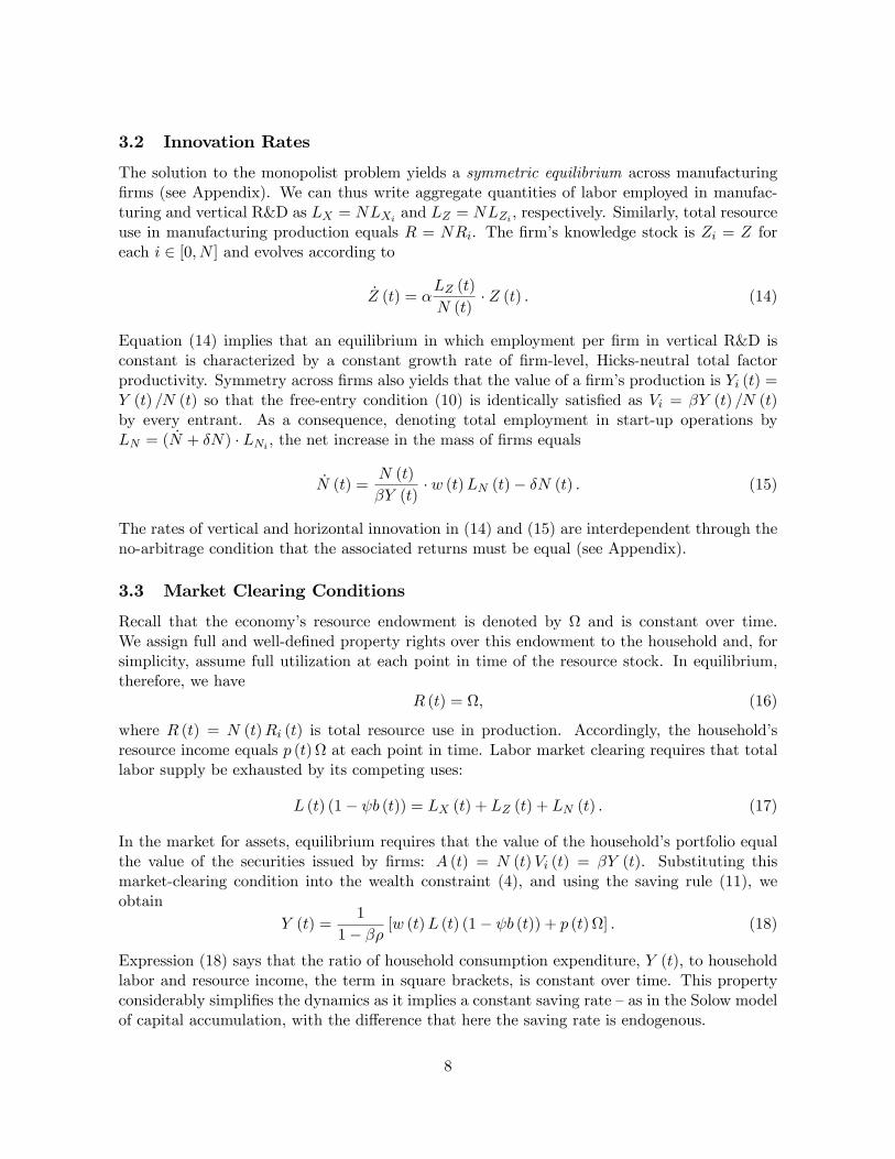
3.2 Innovation Rates

The solution to the monopolist problem yields a symmetric equilibrium across manufacturing�rms (see Appendix). We can thus write aggregate quantities of labor employed in manufac-turing and vertical R&D as LX = NLXi and LZ = NLZi , respectively. Similarly, total resourceuse in manufacturing production equals R = NRi. The �rm�s knowledge stock is Zi = Z foreach i 2 [0; N ] and evolves according to

_Z (t) = �LZ (t)

N (t)� Z (t) : (14)

Equation (14) implies that an equilibrium in which employment per �rm in vertical R&D isconstant is characterized by a constant growth rate of �rm-level, Hicks-neutral total factorproductivity. Symmetry across �rms also yields that the value of a �rm�s production is Yi (t) =Y (t) =N (t) so that the free-entry condition (10) is identically satis�ed as Vi = �Y (t) =N (t)by every entrant. As a consequence, denoting total employment in start-up operations byLN = ( _N + �N) � LNi , the net increase in the mass of �rms equals

_N (t) =N (t)

�Y (t)� w (t)LN (t)� �N (t) : (15)

The rates of vertical and horizontal innovation in (14) and (15) are interdependent through theno-arbitrage condition that the associated returns must be equal (see Appendix).

3.3 Market Clearing Conditions

Recall that the economy�s resource endowment is denoted by and is constant over time.We assign full and well-de�ned property rights over this endowment to the household and, forsimplicity, assume full utilization at each point in time of the resource stock. In equilibrium,therefore, we have

R (t) = ; (16)

where R (t) = N (t)Ri (t) is total resource use in production. Accordingly, the household�sresource income equals p (t) at each point in time. Labor market clearing requires that totallabor supply be exhausted by its competing uses:

L (t) (1� b (t)) = LX (t) + LZ (t) + LN (t) : (17)

In the market for assets, equilibrium requires that the value of the household�s portfolio equalthe value of the securities issued by �rms: A (t) = N (t)Vi (t) = �Y (t). Substituting thismarket-clearing condition into the wealth constraint (4), and using the saving rule (11), weobtain

Y (t) =1

1� �� [w (t)L (t) (1� b (t)) + p (t) ] : (18)

Expression (18) says that the ratio of household consumption expenditure, Y (t), to householdlabor and resource income, the term in square brackets, is constant over time. This propertyconsiderably simpli�es the dynamics as it implies a constant saving rate �as in the Solow modelof capital accumulation, with the di¤erence that here the saving rate is endogenous.

8

4 General Equilibrium Dynamics

For clarity, we split the analysis of general equilibrium dynamics in two parts. First, we studythe interplay between population dynamics and resource scarcity (section 4.1). Second, wedescribe the interaction between horizontal and vertical innovations in determining productivitygrowth (section 4.2). A crucial characteristic of the resulting equilibrium dynamics is theexistence of a steady state displaying constant population.

Henceforth, we take labor as the numeraire and set w (t) � 1 in each instant. In modelswith exogenous population growth, this normalization implies that (nominal) consumptionexpenditure par capita, y (t) � Y (t) =L (t), is constant over time and real growth is representedby the growth rate of the consumption term in the utility function. In the present model,nominal expenditures and production exhibit transitional dynamics due to the endogenousfertility rate. However, in steady state the usual result applies: (nominal) expenditure isconstant and real consumption grows because technological change yields a constant exponentialrate of decay of the consumer price index.

4.1 Fertility and Resource Scarcity

In this subsection we characterize the interactions between population and resource scarcity asa dynamic system involving two variables: the resource endowment per capita and the shadowvalue of humanity. The resource endowment per capita, ! (t) � =L (t), is a state variablethat is given at time zero but is subsequently driven by fertility choices via the dynamics ofpopulation. The shadow value of humanity is denoted by h (t) � ` (t)L (t), where ` (t) is themarginal shadow value of a new worker previously de�ned, and is a forward-looking variabledriving fertility choice under perfect foresight.

We derive the dynamical system in two steps. In section 4.1.1, we treat the values of ! (t)and h (t) as given at time t and derive the equilibrium values of the fertility rate, the resourceprice and consumption expenditure per capita. Building on this result, in section 4.1.2 wederive the two-by-two system that describes the joint dynamics of ! (t) and h (t).

4.1.1 Fertility, Expenditure and Resource Price

The de�nition of h (t) and the optimality condition (12) yield

b (t) =�

y(t) � h (t)

: (19)

Expression (19) shows that the fertility rate is positively related to consumption expenditureper capita, given the shadow value of humanity. Consumption expenditure per capita, in turn,satis�es the equilibrium condition (18), which can be rewritten as

y (t) =1� b (t) + p (t)! (t)

1� �� : (20)

Equation (20) says that consumption expenditure per capita is proportional to the sum oflabor income per capita, 1� b (t), and resource income per capita, p (t)! (t). Resource incomeper capita, in turn, is determined by the equilibrium between the demand for the resource by

9

manufacturing �rms and the household�s supply. Firms�conditional demand for the resource is(see Appendix)

p (t)! (t) = y (t)�� 1�

S (p (t)) ; (21)

where S (p) 2 (0; 1) is the cost share of resource use, i.e., the ratio between total resource rentspaid by manufacturing �rms to resource owners and the total variable costs of manufacturingproduction, and is a function of the resource price. Expression (21) speci�es how expendituredecisions determine resource income through the endogenous resource price. This relationshipdepends on the characteristics of the manufacturing technology (6). Speci�cally, the cost shareof resource use is increasing or decreasing in the resource price depending on the elasticity ofinput substitution (see Appendix):

@S (p)

@p

8<:> 0 if (LXi ; Ri) are complements;< 0 if (LXi ; Ri) are substitutes;= 0 if F (�; �) is Cobb-Douglas.

(22)

The cost-share e¤ect summarized in (22) plays a crucial role in our results.To see this, note that equations (19), (21) and (20) form a static system in three unknowns

that determines the equilibrium levels of p (t), y (t) and b (t) for given levels of the resourceendowment, ! (t), and the shadow value of humanity, h (t). Figure 1 describes graphically theequilibrium determination (see the Appendix for details). In the upper panel, the loci obtainedfrom (20) and (21) determine expenditure given fertility, �y (b (t) ;! (t)). In the lower panel,�y (b (t) ;! (t)) is combined with the locus (19) to determine the equilibrium expenditure andfertility, y� (! (t) ; h (t)) and b� (! (t) ; h (t)). The upper graphs of Figure 1 show that equilibriumexpenditure responds di¤erently to the resource endowment per capita, ! (t), depending onwhether labor and resources are complements or substitutes.5 We summarize the relevantcomparative-statics e¤ects in the following Proposition.

Proposition 1 Given (! (t) ; h (t)) = (!; h) at instant t, there exists a unique triple

fp� (!; h) ; y� (!; h) ; b� (!; h)g

determining the equilibrium levels of the fertility rate, consumption expenditure per capita andthe resource price. Holding h �xed, the marginal e¤ects of an increase in ! are:

(i) Complementarity: @p� (!; h) =@! < 0; @y� (!; h) =@! < 0; @b� (!; h) =@! < 0;(ii) Substitutability: @p� (!; h) =@! < 0; @y� (!; h) =@! > 0; @b� (!; h) =@! > 0;(iii) Cobb-Douglas: @p� (!; h) =@! < 0; @y� (!; h) =@! = 0; @b� (!; h) =@! = 0:

Holding ! �xed, the marginal e¤ects of an increase in h are

@p� (!; h) =@h < 0; @y� (!; h) =@h < 0; @b� (!; h) =@h > 0;

independently of the elasticity of input substitution.5 In graphical terms, an increase in ! implies that the locus y2 �which represents equation (20) � rotates

counter-clock-wise whereas the locus y3 � which represents equation (21) � is una¤ected. Consequently, anincrease in ! induces a decline in �y (b;!) under complementarity (diagram (a)), an increase in �y (b;!) undersubstitutability (diagram (b)), and no e¤ect on �y (b;!) in the Cobb-Douglas case (diagram (c)).

10

Proposition 1 establishes four results. First, the e¤ect of an increase in the resource en-dowment per capita ! on the equilibrium resource price p� is always negative. Second, thee¤ect of ! on equilibrium consumption expenditure per capita y� is negative (positive) if laborand resources are complements (substitutes). The reason is that the sign of the e¤ect of anincrease in ! on on resource income per capita depends on labor-resource substitutability. Un-der complementarity, resource demand is relatively inelastic and an increase in resource supplygenerates a drastic � that is, more than one-for-one � reduction of the price. Consequently,resource income, p!, falls and drives down consumption expenditure. Under substitutability,resource demand is relatively elastic and the increase in ! generates a mild reduction in theresource price, which implies a positive net e¤ect on resource income and thereby higher con-sumption expenditure. In the special Cobb-Douglas case, the price and quantity e¤ects exactlycompensate each other so that resource income and expenditure are not a¤ected by scarcity:@ (p!)� =@! = 0 and @y�=@! = 0.

The third result in Proposition 1 is that b� (!; h) reacts to ! in the same direction asconsumption expenditure: an increase in ! reduces (increases) the fertility rate if labor andresources are complements (substitutes). The reason is the optimality condition (19), whichsays that fertility raises with expenditure per capita for a given shadow value of humanity.The fourth result is that the marginal e¤ects of an increase in h do not depend on inputsubstitutability. On the one hand, the fertility rate is higher the higher is the shadow value ofhumanity. On the other hand, consumption expenditure and the resource price decline becausea higher fertility rate implies reduced work time.

These results play a key role in determining the equilibrium path of the economy: thequalitative characteristics of the transitional dynamics change depending on how income reactsto increased resource scarcity. We address this point by exploiting the instantaneous equilibriumde�ned in Proposition 1 to determine the joint dynamics of ! (t) and h (t).

4.1.2 Dynamic System

From (3), the di¤erential equation describing the equilibrium dynamics of ! (t) is

_! (t) = ! (t) � [d� b� (! (t) ; h (t))] : (23)

Using h (t) � ` (t)L (t), the co-state equation (13) becomes

_h (t) = �h (t)� � � 1� b� (! (t) ; h (t))

y� (! (t) ; h (t)): (24)

The system formed by (23) and (24) allows us to analyze the general equilibrium dynamicsof the resource-population ratio and the associated shadow value of humanity. The results inProposition 1 then allow us to characterize how expenditure per capita, the fertility rate and theresource price evolve along this path. Before studying in detail the properties of system (23)-(24), we complete the description of the general equilibrium dynamics by considering innovationrates and productivity growth.

4.2 Innovations and Productivity Growth

With the wage rate normalized to unity, the model�s relevant measure of real output is theconsumption term in the utility function (2). In equilibrium, therefore, the growth rate of the

11

economy, G (t), is (see Appendix)

G (t) =_y (t)

y (t)� S (p (t)) � _p (t)

p (t)+

(� �

_Z (t)

Z (t)+

1

�� 1 �_N (t)

N (t)

); (25)

where the last term in curly brackets represents the growth rate of total factor productivity(TFP), determined by vertical and horizontal innovations.

From (11) and (3), the equilibrium interest rate is

r (t) = �+_y (t)

y (t)+ b (t)� d: (26)

Note that (25) and (26) imply that in a steady-state equilibrium with constant population,constant expenditure and constant resource price the interest rate equals r (t) = � and the realgrowth rate equals the TFP growth rate.

To determine the dynamics of productivity growth (see the Appendix for details), we notethat in equilibrium the rates of vertical and horizontal innovation �respectively given by (14)and (15) �are jointly determined by a single variable, �rm size, which we denote by x (t) �Y (t) =N (t).

Lemma 2 Along the equilibrium path, the rate of vertical innovation equals

_Z (t)

Z (t)=

�x (t) ��(��1)� � r (t)� � if x (t) > ~x (t)0 if x (t) 6 ~x (t) ; (27)

where~x (t) � �

�� (�� 1) � (r (t) + �) : (28)

Accordingly, the net rate of entry equals

_N (t)

N (t)=1

�

"1

�� 1

x (t)

�+

1

��_Z (t)

Z (t)

!#� �� �: (29)

The existence of the critical �rm size ~x (t) has a clear economic rationale: investing invertical R&D is pro�table only if the �rm�s volume of production is large enough to allow eachproducer to direct the desired portion of earnings to in-house R&D while obtaining a rate ofreturn to vertical innovation that coincides with the prevailing interest rate in the economy.

Lemma 2 implies that the dynamics of the innovation rates can be jointly derived by analyz-ing the equilibrium time path of �rm size, x (t), which is governed by the di¤erential equation

_x (t) =

(�1��(��1)���(r(t)+�)

�� � x (t) + ���r(t)���� if x (t) > ~x (t)

�1���(r(t)+�)�� � x (t) + �

� if x (t) 6 ~x (t): (30)

This expression completes our characterization of equilibrium dynamics. Equation (30) deter-mines the path of �rm size and thereby the paths of vertical and horizontal innovation. Weare particularly interested in the long-run behavior of the productivity growth rate when theeconomy converges to a steady state where expenditure per capita, population and the resourceprice are constant. In this respect, the following result holds:

12

Proposition 3 Suppose that the long-run equilibrium of the economy exhibits limt!1 _y (t) =limt!1 _p (t) = limt!1 _L (t) = 0. Then, the net rate of horizontal innovation is zero and incomegrowth is exclusively driven by vertical innovation,

limt!1

_N (t)

N (t)= 0 and lim

t!1G (t) = � � lim

t!1

_Z (t)

Z (t): (31)

Provided that parameters satisfy � + � < ���(��1)1���(�+�) , the asymptotic �rm size limt!1 x (t) is

above the critical level and the growth rate is strictly positive:

limt!1

G (t) = � � � (�� 1) [��� (�+ �)]1� � (�� 1)� �� (�+ �) � � � (�+ �) > 0: (32)

Proposition 3 incorporates two main results concerning equilibria with constant population.First, economic growth in the long run is exclusively driven by vertical innovation. As discussedin detail elsewhere (Peretto, 1998; Peretto and Connolly, 2007) the process of entry enlarges themass of goods�varieties until the gross entry rate matches the �rms�death rate. Consequently,in the long run the mass of �rms is constant and each �rm invests a constant amount of labor invertical R&D. The second result is that, asymptotically, income growth is independent of factorendowments precisely because net entry eliminates the (strong) scale e¤ect. In the presentmodel, the interaction between horizontal and vertical innovation yields that the economyconverges to a long-run equilibrium with constant population but where (real) income percapita grows at a constant rate. We address this point in detail in the next section.

5 Population, Resources and Technology

5.1 The Pseudo-Malthusian Steady State

Consider a steady state (!ss; hss) in which both the resource per capita and the shadow valueof humanity are constant. Imposing _! = _h = 0 in the dynamic system (23)-(24), we obtain

d = b� (!ss; hss) ; (33)

hss =1

���� +

1� dy� (!ss; hss)

�: (34)

Condition (33) is the obvious requirement of zero net fertility for constant population. Condi-tion (34) de�nes the stationary shadow value of humanity. From Proposition 1, the steady-stateequilibrium (!ss; hss) also implies stationary values for the resource price, consumption expen-diture and the fertility rate, which we denote by (pss; yss; bss). In particular, the long-run levelsof expenditure per capita and population read (see Appendix)

yss = �� (1� d)� + � (�=d)

; (35)

Lss =pss

yss (1� ��)� (1� d) � ; (36)

Recall that by Proposition 3, given the constant values (pss; yss; bss), real income growth equalsthe constant rate of vertical innovation.

13

An important characteristic of this steady state is that yss and Lss are independent oftechnology. From (35), expenditure per capita depends solely on preferences and demographicparameters: neither the endowment of the natural resource, , nor total factor productivityplay any role. From (36), population is proportional to the resource endowment but remainsindependent of technology whereas real income per capita grows at the endogenous rate (32).Therefore, we have a pseudo-Malthusian steady state, that is, a steady state with the Malthusianproperty that resource scarcity limits the population level, but where real income grows at anendogenous rate driven by technological change. It should be clear that a key assumption drivingthis result is that the technological change that drives long-run growth is Hicks-neutral withrespect to labor and land.6 Before pursuing this property further, we need to assess whetherand under what circumstances the pseudo-Malthusian steady state is actually the long-runequilibrium achieved by the economy.

5.2 Stability in the General Case

The stability properties of the pseudo-Malthusian steady state depend on the input elasticity ofsubstitution in manufacturing. We thus have three main cases: complementarity, substitutabil-ity and unit elasticity (Cobb-Douglas). In this section we concentrate on strict complementarityand strict substitutability. We analyze the Cobb-Douglas case in section 5.3 below.

From (35), the pseudo-Malthusian steady state exists whenever � > 1� d. In the (!; h)plane, we denote by h( _!=0) the stationary locus of resource per capita obtained from (23) andby h( _h=0) the stationary locus for the shadow value of humanity obtained from (24). The phasediagrams for the cases of strict substitutability and strict complementarity are in Figure 2 andyield the following result:

Proposition 4 Under substitutability, the stationary loci h( _h=0) and h( _!=0) are decreasing,h(_h=0) cuts h( _!=0) from below, and (!ss; hss) is saddle-point stable. Consequently, the pseudo-

Malthusian steady state is the global attractor of the system and represents the long-run equilib-rium of economy. Under complementarity, the stationary loci are increasing, h( _h=0) cuts h( _!=0)

from above, and (!ss; hss) is an unstable node. Consequently, the pseudo-Malthusian steadystate is a separating threshold: if the resource is initially scarce (abundant) relative to labor,the economy experiences demographic explosion (collapse) in the long run.

Proposition 4 establishes that the pseudo-Malthusian steady state is the long-run equilib-rium of the economy if labor and the resource are substitutes in production. Under complemen-tarity, instead, the steady state is unstable and the economy follows diverging equilibrium pathsleading to population explosion or collapse depending on the relative abundance of resources attime zero. The economic intuition for these results follows from the income e¤ect of resourcescarcity established in Proposition 1.

6 It is of course possible to introduce land-augmenting technological change, as in UGT, but doing so wouldcomplicate the model without adding insight to this paper�s research question. In UGT land-augmenting tech-nological change lifts the economy out of the Malthusian trap by allowing population growth in the phase wherethe subsistence consumption constraint is binding. As explained, our focus is on the future, not the past, andconsequently we do not need to postulate a bias of technological change that puts downward pressure on theland to population ratio.

14

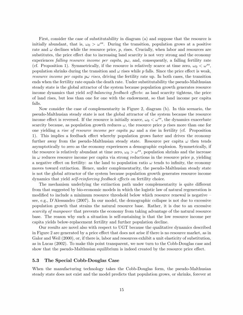
First, consider the case of substitutability in diagram (a) and suppose that the resource isinitially abundant, that is, !0 > !ss. During the transition, population grows at a positiverate and ! declines while the resource price, p, rises. Crucially, when labor and resources aresubstitutes, the price e¤ect due to increasing land scarcity is not very strong and the economyexperiences falling resource income per capita, p!, and, consequently, a falling fertility rate(cf. Proposition 1). Symmetrically, if the resource is relatively scarce at time zero, !0 < !ss,population shrinks during the transition and ! rises while p falls. Since the price e¤ect is weak,resource income per capita p! rises, driving the fertility rate up. In both cases, the transitionends when the fertility rate equals the death rate. Under substitutability the pseudo-Malthusiansteady state is the global attractor of the system because population growth generates resourceincome dynamics that yield self-balancing feedback e¤ects: as land scarcity tightens, the priceof land rises, but less than one for one with the endowment, so that land income per capitafalls.

Now consider the case of complementarity in Figure 2, diagram (b). In this scenario, thepseudo-Malthusian steady state is not the global attractor of the system because the resourceincome e¤ect is reversed. If the resource is initially scarce, !0 < !ss, the dynamics exacerbatescarcity because, as population growth reduces !, the resource price p rises more than one forone yielding a rise of resource income per capita p! and a rise in fertility (cf. Proposition1). This implies a feedback e¤ect whereby population grows faster and drives the economyfurther away from the pseudo-Malthusian steady state. Resource per capita ! then tendsasymptotically to zero as the economy experiences a demographic explosion. Symmetrically, ifthe resource is relatively abundant at time zero, !0 > !ss, population shrinks and the increasein ! reduces resource income per capita via strong reductions in the resource price p, yieldinga negative e¤ect on fertility: as the land to population ratio ! tends to in�nity, the economymoves toward extinction. Hence, under complementarity, the pseudo-Malthusian steady stateis not the global attractor of the system because population growth generates resource incomedynamics that yield self-reinforcing feedback e¤ects on fertility choice.

The mechanism underlying the extinction path under complementarity is quite di¤erentfrom that suggested by bio-economic models in which the logistic law of natural regeneration ismodi�ed to include a minimum resource threshold below which resource renewal is negative �see, e.g., D�Alessandro (2007). In our model, the demographic collapse is not due to excessivepopulation growth that strains the natural resource base. Rather, it is due to an excessivescarcity of manpower that prevents the economy from taking advantage of the natural resourcebase. The reason why such a situation is self-sustaining is that the low resource income percapita yields below-replacement fertility and further population decline.

Our results are novel also with respect to UGT because the qualitative dynamics describedin Figure 2 are generated by a price e¤ect that does not arise if there is no resource market, as inGalor and Weil (2000), or, if there is, labor and resources exhibit a unit elasticity of substitution,as in Lucas (2002). To make this point transparent, we now turn to the Cobb-Douglas case andshow that the pseudo-Malthusian equilibrium is indeed created by the resource price e¤ect.

5.3 The Special Cobb-Douglas Case

When the manufacturing technology takes the Cobb-Douglas form, the pseudo-Malthusiansteady state does not exist and the model predicts that population grows, or shrinks, forever at

15

a constant rate. The proof follows from Proposition 1. A unit elasticity of input substitutionimplies that neither expenditures nor the fertility rate are a¤ected by variations in resourcesper capita. Consequently, the stationary loci h( _!=0) and h( _h=0) become horizontal straight linesin the (!; h) plane. The properties of the dynamic system (23)-(24) fall in three subcases: (i)the locus h( _!=0) lies below h(

_h=0), (ii) the locus h( _!=0) lies above h( _h=0), or (iii) the two locicoincide.

Figure 3 describes the phase diagram (see the Appendix for details) in all subcases. Thecommon characteristic is that, given the initial condition ! (0) = !0, the shadow value of hu-manity jumps on the h( _h=0) locus at time zero.7 In subcase (i) there is no pseudo-Malthusianequilibrium: given !0, the economy moves along the h(

_h=0) locus and population grows at aconstant exponential rate during the whole transition.8 Subcase (ii) is specular: the economymoves along the h( _h=0) locus with a permanently declining level of population, with no tran-sitional dynamics in the fertility rate because the shadow value of humanity is constant. Insubcase (iii), the parameters of the model are such that the the equilibrium fertility rate ex-actly coincides with the exogenous mortality rate. However, this steady state is di¤erent fromthe pseudo-Malthusian equilibrium as there are no interactions between resource scarcity andfertility over time: the economy maintains the intial resource endowment per capita !0 forever.

6 Minimum Resource Requirement: A Preventive Check

A question that arises naturally is whether the prediction of stable population in the longrun �which holds under substitutability �extends to the cases of complementarity and unitsubstitution if we further enrich the model. In particular, considering the equilibrium pathsyielding ! (t) ! 0, what kind of forces may stop the demographic explosion? In this sectionwe present a simple extension of the model that yields a considerable generalization of ourresults. Speci�cally, we assume that each adult has a �xed minimum requirement of the resourceand show that this induces a congestion e¤ect that operates through the price of land p andampli�es the preventive check against demographic explosion making it the dominant force forany elasticity of substitution between labor and land.

6.1 Equilibrium with Minimum Requirement

We denote the �xed requirement of resource per adult by �, and impose

! (t) > � in each t 2 [0;1) : (37)

This assumption can be rationalized in many ways. For example, if the resource representstotal available land, constraint (37) establishes that there is a minimum land requirement �e.g., residential land �for each adult. Setting � = 0, we are back to the original model analyzedin the previous sections.

7All explosive paths yielding h (t)!1 or h (t) < 0 at some �nite date are ruled out by standard arguments:they either violate the transversality condition limt!1 h (t) e��t = 0 or the household�s budget constraint in�nite time.

8The population growth rate is constant because the shadow value of humanity is constant. Since expenditureis not a¤ected by variations in resource per capita (cf. Proposition 1), having _h = 0 implies a constant fertilityrate b (t) by virtue of condition (19). The same reasoning applies to all subcases.

16

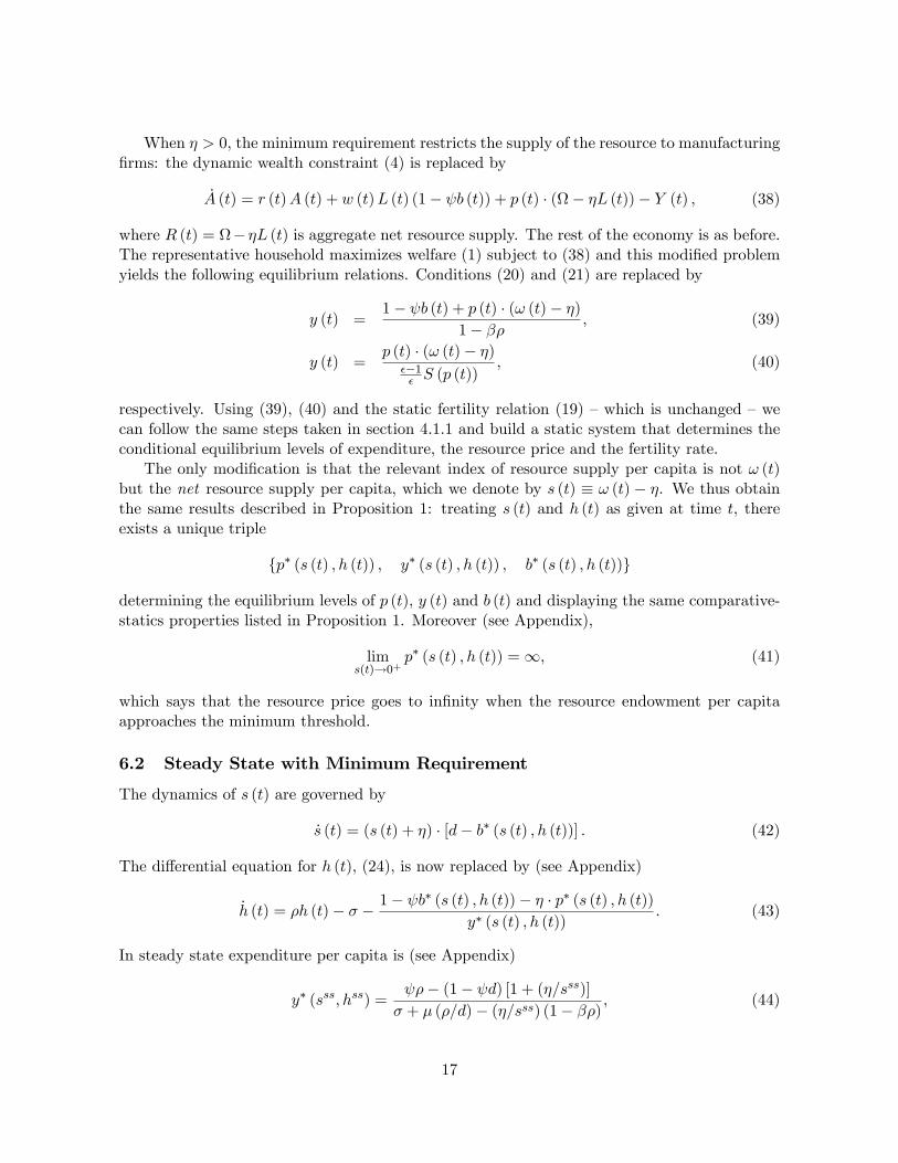
When � > 0, the minimum requirement restricts the supply of the resource to manufacturing�rms: the dynamic wealth constraint (4) is replaced by

_A (t) = r (t)A (t) + w (t)L (t) (1� b (t)) + p (t) � (� �L (t))� Y (t) ; (38)

where R (t) = ��L (t) is aggregate net resource supply. The rest of the economy is as before.The representative household maximizes welfare (1) subject to (38) and this modi�ed problemyields the following equilibrium relations. Conditions (20) and (21) are replaced by

y (t) =1� b (t) + p (t) � (! (t)� �)

1� �� ; (39)

y (t) =p (t) � (! (t)� �)

��1� S (p (t))

; (40)

respectively. Using (39), (40) and the static fertility relation (19) �which is unchanged �wecan follow the same steps taken in section 4.1.1 and build a static system that determines theconditional equilibrium levels of expenditure, the resource price and the fertility rate.

The only modi�cation is that the relevant index of resource supply per capita is not ! (t)but the net resource supply per capita, which we denote by s (t) � ! (t) � �. We thus obtainthe same results described in Proposition 1: treating s (t) and h (t) as given at time t, thereexists a unique triple

fp� (s (t) ; h (t)) ; y� (s (t) ; h (t)) ; b� (s (t) ; h (t))g

determining the equilibrium levels of p (t), y (t) and b (t) and displaying the same comparative-statics properties listed in Proposition 1. Moreover (see Appendix),

lims(t)!0+

p� (s (t) ; h (t)) =1; (41)

which says that the resource price goes to in�nity when the resource endowment per capitaapproaches the minimum threshold.

6.2 Steady State with Minimum Requirement

The dynamics of s (t) are governed by

_s (t) = (s (t) + �) � [d� b� (s (t) ; h (t))] : (42)

The di¤erential equation for h (t), (24), is now replaced by (see Appendix)

_h (t) = �h (t)� � � 1� b� (s (t) ; h (t))� � � p� (s (t) ; h (t))

y� (s (t) ; h (t)): (43)

In steady state expenditure per capita is (see Appendix)

y� (sss; hss) = �� (1� d) [1 + (�=sss)]

� + � (�=d)� (�=sss) (1� ��) ; (44)

17

where sss indicates the constant level of net resource supply per capita associated to the constantlevel of the shadow value of humanity hss.

Denote by h( _s=0) and h( _h=0) the stationary loci determined by (42) and (43) in the (s; h)plane. The di¤erence with respect to the original model with � = 0 is that the locus h( _h=0)

exhibits a vertical asymptote in h = 0 and goes to minus in�nity independently of the elasticityof substitution. This result is described in the upper panel of Figure 4, where we consider (a)substitutability, (b) complementarity and (c) the Cobb-Douglas case for the relevant subcasefeaturing growing population.9 Starting from � = 0, and subsequently imposing higher valuesof �, the left branch of the locus h( _h=0) bends downward and the locus shifts down. As one cansee, the congestion e¤ect due to the minumum land requirement per capita removes ! = 0 asa possible attractor of the system and, for technologies that feature elasticity of susbstitutionless than or equal to one, replaces it with one that features constant population.

The intuition is provided by result (41) combined with the costate equation (43). Whenthe amount of resource per capita approaches the minimum requirement, the resource priceexplodes to in�nity. This force shows up in fertility choices as the term � � p (s; h) in equation(43) that governs the dynamics of the shadow value of humanity: although, as in the baselinemodel with � = 0, our representative household experiences an exploding resource income percapita, it now responds to the exploding respource price by lowering fertility because it nowknows that that exploding price signals excessive congestion of the resource.

6.3 Dynamics with Minimum Requirement

Figure 4 clari�es the consequences of the minimum resource requirement for the number ofsteady states and their stability properties. Under substitutability, our conclusions do notchange: as shown in diagram (d), the steady state (sss; hss) is unique and is saddle-point stablebecause h( _h=0) cuts h( _s=0) from below.

Under complementarity, instead, two steady states arise. As shown in diagram (e), thereare is a �low�pseudo-Malthusian equilibrium, denoted by (s0ss; h

0ss), as well as a �high�pseudo-

Malthusian equilibrium, denoted by (s00ss; h00ss). The �high�equilibrium is an unstable node and

thus acts as a separating threshold. The �low�equilibrium, instead, is saddle-path stable andis therefore the local attractor of the system. Provided that the initial net resource endowmentis below s00ss, the economy converges to the pseudo-Malthusian steady state (s

00ss; h

00ss).

Consider now the Cobb-Douglas case. In the original model with � = 0 the economy followsa path of constant exponential growth of population (cf. Figure 3, subcase (i)). The positiverequirement � > 0 generates a unique pseudo-Malthusian steady state that is saddle-path stableand is thus the global attractor of the system; see Figure 4, diagram (f). We summarize theseconclusions as follows.

Proposition 5 Given a �xed requirement of resource per adult � > 0, the economy convergestowards a pseudo-Malthusian steady state under substitutability, under complementarity (pro-vided that s0 < s00ss) and under Cobb-Douglas technology (subcase (i)).

9 In the Cobb-Douglas scenario, we limit our attention to subcase (i) because it is the only case featuringdemographic explosion (cf. Figure 3). The introduction of a minimum resource requirement is only relevant forequilibrium paths that exhibit the inherent tendency to zero resource per capita in the long run.

18

With the inclusion of a congestion e¤ect due to a minimum resource requirement that mimicsthe role of residential land, our theory of the long-run level of population appears robust withrespect to scenarios in which labor and resources are not strictly substitutes: the preventive-check mechanism driven by the price of land always eliminates explosive population dynamics.

7 Conclusion

This paper investigated the links between resource scarcity, income levels and population growthin a Schumpeterian model with endogenous fertility. Our analysis o¤ers the following results.When labor and resources are strict complements or strict substitutes in production, the in-crease in resource scarcity induced by population growth generates price e¤ects that modifyincome per capita yielding feedback e¤ects on fertility. These price e¤ects create a pseudo-Malthusian equilibrium in which population is constant, income per capita grows at a constantendogenous rate and population size is independent of technology. Under substitutability, thisequilibrium is a global attractor and indeed determines the population level in the long run:increased resource scarcity reduces income producing self-balancing e¤ects on population viareduced fertility. Under complementarity, instead, the pseudo-Malthusian equilibrium acts as aseparating threshold and population level follows diverging paths: increased (reduced) resourcescarcity generated by the growth (decline) of population increases (decreases) income per capitaand fertility rates, implying self-reinforcing feedback e¤ects that drive the economy towards de-mographic explosion (human extinction). If we introduce a minimum resource requirementper adult �e.g., residential land �the economy avoids demographic explosion in all scenarios.Agents internalize the minimum requirement in intertemporal choices and this preventive checkgenerates stable pseudo-Malthusian equilibria: population achieves a stationary level in thelong run even under complementarity.

Our analysis unveils a theory of interactions between resources and population that di¤ers inseveral respects from the existing literature. Price e¤ects are generally neglected in the literatureon Uni�ed Growth Theory, which typically assumes a unit elasticity of substitution betweenlabor and resources. Also, the model predictions di¤er from those of bio-economic models: ifwe consider the extinction path arising under complementarity, the collapse of the society is notdue to excessive natural scarcity �as in models where natural regeneration becomes negativebelow a certain stock threshold �but rather to the continuous decline in resource prices whichreduces expenditures, incomes and fertility. More generally, our analysis suggests a theory ofthe population level which is consistent with the fact that Planet Earth has a �nite carryingcapacity of people. This basic characteristic of closed systems is not captured by standardbalanced growth models, that typically predict exponential population growth in the long run.

A Appendix

Household problem: derivation of (11), (12), (13). In the �rst step, the householdmaximizes (2) subject to (5). The solution yields the demand schedule for product i,

Xi (t) = Y (t)Pi (t)

��R N(t)0 Pi (t)

1�� di: (A.1)

19

Atomistic �rms take the denominator of (A.1) as given and each monopolist faces an isoelasticdemand curve. Plugging (A.1) in (A.1), indirect instantaneous utility reads

log u(t) = ~u+ log (Y (t) =L (t)) + � log b (t) + (� + 1) logL (t) (A.2)

where ~u is a function of the goods�prices (taken as given). Expression (A.2) implies a positivenet elasticity of utility to population, � > 0. In the second step, the household maximizes(1) subject to (4) and (3) using Y and b as control variables and A and L as state variables.Plugging (A.2) in (1), the Hamiltonian for this problem reads

LH � ~u+ log Y + � log b+ � logL+ � � [rA+ wL (1� b) + pR� Y ] + ` � [L (b� d)] ; (A.3)

where � and ` are the dynamic multipliers associated to A and L, respectively. The optimalityconditions read

1=Y (t) = � (t) ; (A.4)

�=b (t) = � (t)w (t)L (t)� ` (t)L (t) ; (A.5)

�� (t)� _� (t) = � (t) r (t) ; (A.6)

�` (t)� _̀ (t) = (�=L (t)) + � (t)w (t) (1� b (t)) + ` (t) � (b (t)� d) ; (A.7)

in addition to the usual transversality conditions

limt!1

� (t)A (t) e��t = limt!1

` (t)L (t) e��t = 0: (A.8)

Combining (A.4) with (A.6), we obtain (11). Substituting (A.4) in (A.5) and solving for ` (t),we obtain (12). Using (A.4) to eliminate � (t) from (A.7), we obtain equation (13) in the text.

The monopolist problem. The instantaneous pro�t of the i-th monopolist is

�i = PiXi � wLXi � pRi � wLZi : (A.9)

From (6), the cost-minimizing combination of LXi and Ri, for given wage w and resource pricep, yields total production costs

w�+ C(w; p)Z��i Xi; (A.10)

where C (�) is the unit-cost function homogeneous of degree one. Using (A.10), instantaneouspro�ts (A.9) can be re-written as

�i = [Pi � C(w; p)Z��i ]Xi � w�� wLZi ; (A.11)

where Pi is the market price of the produced variety. In the �rst step, the monopolist maximizes(A.11) subject to the demand schedule (A.1) �taking the denominator as given �obtaining themark-up rule

Pi =�

�� 1 � C(w; p)Z��i for each i 2 [0; N ] : (A.12)

In the second step, the �rm maximizes (9) subject to (7). Using (A.11), the current-valueHamiltonian for the i-th �rm reads

LMi � [Pi � C(w; p)Z��i ]Xi � w�� wLZi + �i�KLZi ;

20

where �i is the dynamic multiplier attached to �rm-speci�c knowledge. The state variable isZi, the control variable is R&D employment, LZi , and the public knowledge stock, K, is takenas given. The �rst order conditions for the interior solution are given by

�i�K = w (A.13)

r + � � �C(w; p)Z���1i

Xi

�i=

_�i�i; (A.14)

limv!1

e�R vt [r(v

0)+�]dv0�i(v)Zi(v) = 0: (A.15)

Peretto (1998, Proposition 1) shows that, under the restriction 1 > � (�� 1), the �rm is alwaysat the interior solution, where w = �i�K holds and equilibrium is symmetric.10

Innovation rates and no-arbitrage. Symmetry across manufacturing �rms implies K =Z = Zi and thereby _K=K = �LZ=N , where LZ is aggregate employment in vertical R&D.Also, the free-entry condition (10) reduces to Vi = �Y (t) =N (t) by every i-th entrant in themanufacturing business. Time-di¤erentiating (9), we have

r (t) + � =�Xi (t)

Vi (t)+_Vi (t)

Vi (t); (A.16)

which is a perfect-foresight, no-arbitrage condition for the equilibrium in the capital market.The rates of return to vertical and horizontal R&D read

r (t) = rZ (t) �_w (t)

w (t)+ �

��(�� 1)

�� Y (t)

N (t)w (t)� LZ (t)

N (t)

�� �; (A.17)

r (t) = rN (t) �1

�

�1

�� N (t)w (t)

Y (t)

��+

LZ (t)

N (t)

��+_Y (t)

Y (t)�

_N (t)

N (t)� �; (A.18)

respectively. Equation (A.17), is obtained by time-di¤erentiating (A.13) and using the demandcurve (A.1), the R&D technology (7) and the price strategy (A.12). Equation (A.18) followsfrom substituting Vi = �Y=N in (A.16). No-arbitrage requires that rZ (t) = rN (t) in eachinstant t.

Conditional input demands: derivation of (21) and (22). The cost function (A.10)gives rise to the conditional factor demands

LXi =@C (w; p)

@wZ��i Xi + � and Ri =

@C(w; p)

@pZ��i Xi (A.19)

for each �rm i. Combining (A.19) with the price strategy (A.12), and aggregating across �rmsunder symmetry, we obtain the aggregate demand schedules

LX (t) = Y (t)�� 1�

h1� ~S (w (t) ; p (t))

i+ �N (t) ; (A.20)

R (t) = Y (t)�� 1�

~S (w (t) ; p (t))

p (t); (A.21)

10Because the Hamiltonian is linear in LZi , we may have three cases. If �i�K < w, the value of the marginalunit of knowledge is below its cost and the �rm does not invest. If �i�K > w, the value of the marginal unitof knowledge exceeds its cost: this case is ruled out as it violates the general equilibrium conditions (the �rmwould demand an in�nite amount of labor for R&D purposes).

21

where ~S (w; p) is the resource share in the �rm�s total variable cost:

~S (w; p) � pRi

C(w; p)Z��i Xi

=@ logC(w; p)

@ log p: (A.22)

Normalizing the wage rate w (t) = 1 in each instant t, the cost function reduces to C(w; p) =C(1; p) and the resource cost share can be re-de�ned as

S (p) � ~S (1; p) =@ logC(1; p)

@ log p: (A.23)

Because the resource cost share S (p) equals the elasticity of the cost function with respect tothe resource price, it exhibits the properties reported in (22) as well as

(i) Complementarity: limp!0 S (p) = 0; limp!1 S (p) = 1;(ii) Substitutability: limp!0 S (p) = 1; limp!1 S (p) = 0;(iii) Cobb-Douglas: S (p) = �S 2 (0; 1) :

(A.24)

Multiplying both sides of (A.21) by p (t) =L (t) and substituting R (t) = from (16), we obtainequation (21) in the text.

Proof of Proposition 1. Eliminating time-arguments and treating (!; h) as parameters,the system formed by (19), (20) and (21) can be rewritten as

y1 (b;h) �

h+ (�=b); (A.25)

y2 (b; p;!) � 1� b1� �� +

!

1� �� � p; (A.26)

y3 (b; p) � 1� b1� ��� ��1

� S (p); (A.27)

where (A.27) is obtained by plugging (21) in (20) to eliminate p! and solving for y. Theproof of Proposition 1 involves three steps. First, we prove the existence and uniqueness of theequilibrium. Second, we assess the marginal e¤ects of variations in !. Third, we assess themarginal e¤ects of variations in h.

Step #1. The subsystem formed by (A.26) and (A.27) can be represented graphically in the(p; y) plane: given b and !, function y2 (b; p;!) is a linear increasing function of p, whereas thebehavior of y3 (b; p) depends on the elasticity of substitution: from (22), it is (i) increasing andconcave under complementarity; (ii) decreasing and convex under substitutability; (iii) a �athorizontal line in the Cobb-Douglas case. The three cases are respectively described in diagrams(a), (b) and (c) of Figure 1. The vertical intercepts and horizonal aymptotes of y3 (b; p) arede�ned in (A.24) and (A.27). In all cases, the intersection y2 (b; p;!) = y3 (b; p) is uniqueand determines the conditional values �y (b;!) and �p (b;!). In particular, �y (b;!) exhibits theproperty

ymin (b) �1� b1� �� < �y (b;!) <

1� b1� ��� ��1

�

� ymax (b) : (A.28)

In all cases, a ceteris paribus increase in b shifts down the vertical intercept of y2 (b; p;!) as wellas the vertical intercept and the horizontal asymptotes of y3 (b; p). This implies that �y (b;!) is

22

monotonically decreasing in b with

@

@b�y (b;!) < 0; lim

b!0�y (b;!) = �y (0;!) > 0; lim

b!1= �y (b;!) = 0: (A.29)

Reporting the �y (b;!) locus in the (b; y) plane in the three cases, we respectively obtain diagrams(d), (e) and (f) in Figure 1. In the same diagrams, we plot the y1 (b;h) schedule de�ned in (A.25),which is strictly increasing and concave in b. In all cases, the intersection �y (b;!) = y1 (b;h) isunique and thus determines a unique couple of equilibrium values, b� (!; h) and y� (!; h). Givenb� (!; h) and y� (!; h), there exists a unique value of the resource price p� (!; h) satisfying themonotonous relation (A.26).

Step #2. The marginal e¤ects of ! can be studied by means of Figure 1. In all cases, anincrease in ! increases the slope of y2 (b; p;!) leaving y3 (b; p) unchanged, so that

@�p (b;!)

@!< 0; lim

!!0+�p (b;!) =1; lim

!!1�p (b;!) = 0; (A.30)

independently of the elasticity of substitution. With respect to �y (b;!), we have to considereach case in turn. Under complementarity, the positive e¤ect of ! on the slope of y2 (b; p;!)implies

(Compl.):@�y (b;!)

@!< 0; lim

!!0+�y (b;!) = ymax (b) ; lim

!!1�y (b;!) = ymin (b) (A.31)

Result (A.31) implies that, in diagram (d) of Figure 1, the �y (b;!) schedule moves down rotatingcounter-clockwise around the horizontal intercept b = 1=!. We thus have @

@!y� (!; h) < 0 and

@@! b

� (!; h) < 0. From the equilibrium relation (A.27) evaluated in the equilibrium, the signs@@!y

� (!; h) < 0 and @@! b

� (!; h) < 0 require

@S (p� (!; h))

@!=@S (p)

@p� @p

� (!; h)

@!< 0;

which �given @S (p) =@p > 0 �implies @@!p

� (!; h) < 0. Now consider the case of substitutability :the positive e¤ect of ! on the slope of y2 (b; p;!) implies

(Subs.):@�y (b;!)

@!> 0; lim

!!0+�y (b;!) = ymin (b) ; lim

!!1�y (b;!) = ymax (b) ; (A.32)

Result (A.32) implies that, in diagram (e) of Figure 1, the �y (b;!) schedule moves up rotat-ing clockwise around the horizontal intercept b = 1=!. We thus have @

@!y� (!; h) > 0 and

@@! b

� (!; h) > 0. From the equilibrium relation (A.27) evaluated in the equlibrium, the signs@@!y

� (!; h) > 0 and @@! b

� (!; h) > 0 require

@S (p� (!; h))

@!=@S (p)

@p� @p

� (!; h)

@!> 0;

which �given @S (p) =@p < 0 �implies @@!p

� (!; h) < 0. Next consider the Cobb-Douglas case:the positive e¤ect of ! on the slope of y2 (b; p;!) yields a decline in �p (b;!) but no e¤ect on

23

conditional expenditure, @@! �y (b;!) = 0. This implies that, in diagram (f) of Figure 1, the

�y (b;!) schedule is the horizontal line

(Cobb-Douglas): �y (b;!) =1� b

1� ��� ��1��S; (A.33)

obtained by substituting the constant S (p) = �S 2 (0; 1) in (A.27). Hence, we get @@!y

� (!; h) =

0 and @@! b

� (!; h) = 0. The only e¤ect of ! is on the resource price, which is negative:@@!p

� (!; h) = @@! �p (b;!) < 0.

Step #3. From de�nition (A.23), the combined function � (p) � p=S (p) exhibits

@� (p)

@p> 0; lim

p!0� (p) = 0; lim

p!1� (p) =1; (A.34)

and allows us to rewrite the equilibrium relation (21) as

y� (!; h) = ! � �

�� 1 � � (p� (!; h)) : (A.35)

The marginal e¤ects of h can be studied by means of diagrams (d), (e) and (f) in Figure 1. Inall cases, an increase in h leaves the �y (b;!) schedule unchanged whereas the y1 (b;h) schedulede�ned in (A.25) exhibits

@y1 (b;h)

@h< 0; lim

h!0+y1 (b;h) =

�b; lim

h!1y1 (b;h) = 0: (A.36)

Result (A.36) implies that y1 (b;h) moves down rotating clockwise around the origin as h in-creases. Consequently, we have @

@hb� (!; h) > 0 and @

@hy� (!; h) < 0 independently of the

elasticity of substitution. The e¤ect of h on the resource price is obtained by di¤erentiating(A.35) with respect to h, which yields

@

@hy� (!; h) = !

�

�� 1 �@�

@p� @p

� (!; h)

@h:

Since @�=@p > 0 independently of the elasticity of substitution, the sign of @@hp

� (!; h) is alwaysthe same as that of @

@hy� (!; h) < 0. �

Derivation of (25). By symmetry in the manufacturing sector, substitute Xi = X foreach i 2 [0; N ], the demand function (A.1), and the price strategy (A.12), in the consumptionterm of the utility function (2) to obtain"Z N(t)

0

�Xi (t)

L (t)

� ��1�

di

# ���1

=y (t)

Pi (t)N (t)

1��1 =

�� 1�

� y (t)

C(1; p (t))Zi (t)

�N (t)1��1 ; (A.37)

where we have used Zi (t) = Z (t) and C(w (t) ; p (t)) = C (1; p (t)). Recalling that S (p) �@ logC(1;p)@ log p by de�ntion (A.23), the growth rate of (A.37) is given by (25).Proof of Lemma 2. Setting w (t) = 1 and Y (t) =N (t) in (A.17), and using (14) to

eliminate LZ=N , we obtain

_Z (t) =Z (t) = x (t) � (�=�) � � (�� 1)� r (t)� �;

24

which is (strictly) positive if and only if �rm size (strictly) exceeds ~x (t) de�ned in (28). Thisproves result (27). From (A.18), we have

r (t) =1

�

"1

�� 1

x (t)

�+

1

��_Z (t)

Z (t)

!#+_Y (t)

Y (t)�

_N (t)

N (t)� �: (A.38)

Plugging r (t) = �+ _Y (t) =Y (t) from (11) and solving the resulting expression for _N (t) =N (t),we obtain (29).

Derivation of (30). From (A.38), the growth rate of �rm size equals

_x (t)

x (t)=_Y (t)

Y (t)�

_N (t)

N (t)= r (t) + � � 1

�

"1

�� 1

x (t)

�+

1

��_Z (t)

Z (t)

!#;

where we can substitute (27) and solve for _x (t) in the two cases, x (t) > ~x (t) and x (t) 6 ~x (t),to obtain (30).

Proof of Proposition 3. If limt!1 _y (t) = limt!1 _p (t) = limt!1 _L (t) = 0, equations(25) and (26) respectively imply

limt!1

G (t) = � �_Z (t)

Z (t)+

1

�� 1 �_N (t)

N (t); (A.39)

limt!1

r (t) = �: (A.40)

Substituting (A.40) in (28), the asymptotic critical threshold for obtaining positive verticalinnovations is

limt!1

x (t) > ~x (1) � � (�+ �)

�� (�� 1) : (A.41)

Consequently, from (30), we have two possible steady-state levels for �rm size,

limt!1

x (t) =

((�=�) � ���(�+�)

1��(��1)���(�+�) if �+ � < ���(��1)1���(�+�)

��1���(�+�) if �+ � > ���(��1)

1���(�+�); (A.42)

where � + � < ���(��1)1���(�+�) implies strictly positive vertical innovations and � + � > ���(��1)

1���(�+�)implies, instead, constant Z (t) in the long run. Substituting (A.42) in (27), we have

limt!1

_Z (t)

Z (t)=

(�(��1)[���(�+�)]1��(��1)���(�+�) � (�+ �) if �+ � < ���(��1)

1���(�+�)0 if �+ � > ���(��1)

1���(�+�); (A.43)

where the case of operative vertical R&D does not require any further restriction on parameters.Plugging (A.43) in (29), we also have

limt!1

_N (t)

N (t)=

(0 if �+ � < ���(��1)

1���(�+�)0 if �+ � > ���(��1)

1���(�+�): (A.44)

Using (A.39), results (A.43) and (A.44) imply (31) and (32). �

25

Derivation of (35) and (36). Using (33) and (34) to eliminate bss and hss from theequilibrium conditions (19) and (20), respectively, we obtain expressions (35) and (36) in thetext.

Proof of Proposition 4. Proposition 4 is proved in three steps. First, we show thatthe stationary loci h( _!=0) and h( _h=0) are both increasing (decreasing) in the (!; h) plane undercomplementarity (substitutability), and are both horizontal straight lines in the special Cobb-Douglas case. Second, we show that under substitutability (complementarity), h( _h=0) cutsh( _!=0) from below (above). Third, we show that under substitutability (complementarity), thesteady state (!ss; hss) is a stable saddle-point (unstable node or focus).

Step #1. Equation (35) and condition (A.27) evaluated at (yss; bss) imply

� + � (�=d) = �� (1� d)

1� d ��1� ��� �� 1

�S (p)

�(A.45)

For future reference, de�ne the constants

�0 � 1� ����� 1�

and �1 � 1� ��; (A.46)

where �0 < �1. Imposing _! = 0 in (23), the resulting locus h( _!=0) is characterized by b� (!; h) =d. From the Proof of Proposition 1, we know that, given b� (!; h) = d, the equilibrium ischaracterized by the conditional values �y (b;!) and �p (b;!) determined in Figure 1 and evaluatedin b = d. In particular, results (A.31), (A.32) and (A.33) respectively imply the three cases8>>><>>>:

Comp: @�y(d;!)@! < 0; lim

!!0�y (d;!) = 1� d

�0; lim

!!1�y (d;!) = 1� d

�1;

Subs: @�y(b;!)@! > 0; lim

!!0�y (d;!) = 1� d

�1; lim

!!1�y (d;!) = 1� d

�0;

C-D: @�y(b;!)@! = 0; �y (d;!) = 1� d

1���� ��1��S:

9>>>=>>>; (A.47)

From (19), given b� (!; h) = d, the locus h( _!=0) is represented by

h( _!=0) =

y� (!; h)� �

b� (!; h)=

�y (d;!)� �

d: (A.48)

Plugging results (A.47) in (A.48), we obtain8>>><>>>:Comp: @h( _!=0)

@! > 0; lim!!0

h( _!=0) = �01� d �

�d ; lim

!!1h( _!=0) = �1

1� d ��d ;

Subs: @h( _!=0)

@! < 0; lim!!0

h( _!=0) = �11� d �

�d ; lim

!!1h( _!=0) = �0

1� d ��d ;

C-D: @h( _!=0)

@! = 0; h( _!=0) = (1���� ��1

��S)

1� d � �d :

9>>>=>>>; (A.49)

Now consider the locus h( _h=0). From (24), we have

h(_h=0) =

1

�

�� +

1� b� (!; h)y� (!; h)

�=1

�

�1� ��� �� 1

�S (p� (!; h)) + �

�; (A.50)

where we have used condition (A.27) evaluated in equilibrium to obtain the last term. Using theproperties of S (p) listed in (22) and (A.24), as well as the result @

@!p� (!; h) < 0 in Proposition

26

1, we have8>>><>>>:Comp: @h(

_h=0)

@! > 0; lim!!0

h(_h=0) = �0+�

� ; lim!!1

h(_h=0) = �1+�

� ;

Subs: @h(_h=0)

@! < 0; lim!!0

h(_h=0) = �1+�

� ; lim!!1

h(_h=0) = �0+�

� ;

C-D: @h(_h=0)

@! = 0; h(_h=0) = 1

�

�1� ��� ��1

��S + �

�:

9>>>=>>>; (A.51)

Results (A.49) and (A.51) imply that both h( _!=0) and h( _h=0) are increasing (decreasing) in the(!; h) plane under complementarity (substitutability) while they are both horizontal straightlines in the Cobb-Douglas case.

Step #2. Denote by � (0) the distance between the vertical intercepts of h( _!=0) and h( _h=0)

and, similarly, denote by � (1) the vertical distance between the asymptotic levels of h( _!=0)and h( _h=0) as ! !1, i.e.,

� (0) � lim!!0

h( _!=0) � lim!!0

h(_h=0) and � (1) � lim

!!1h( _!=0) � lim

!!1h(_h=0): (A.52)

First, consider the case of complementarity. From (A.49) and (A.51), we have

Comp: � (0) =1

�

� �� (1� d)

1� d � �0 � � � � (�=d)�:

Substituting (A.45) and recalling the de�nition of �0 in (A.46), the above expression reducesto

Comp: � (0) = �1�� �� (1� d)

1� d � �� 1�

� (1� S (pss)) < 0: (A.53)

Similarly, calculating � (1) from (A.49) and (A.51), using (A.45) and (A.46) to eliminate �1,we get

Comp: � (1) = 1

�� �� (1� d)

1� d � �� 1�

� S (pss) > 0: (A.54)

Results (A.53)-(A.54) imply that, under complementarity, h( _h=0) cuts h( _!=0) from above. Re-peating the same steps for the case of substitutability, we obtain the symmetric results

Subs: � (0) =1

�� �� (1� d)

1� d � �� 1�

� S (pss) > 0; (A.55)

Subs: � (1) = �1�� �� (1� d)

1� d � �� 1�

� (1� S (pss)) < 0; (A.56)

so that, under substitutability, h( _h=0) cuts h( _!=0) from below.Step #3. Linearizing system (23)-(24) around (!ss; hss), we obtain�

_!_h

�'�m1 m2

m3 m4

��(! � !ss)(h� hss)

�; (A.57)

where the coe¢ cient matrix is

m1 � �!ss � @b(!;h)@!

���!=!ss

and m2 � �!ss � @b(!;h)@h

���h=hss

;

m3 � ��1� � @

@!S (p� (!; h))

��!=!ss

and m4 � �+ ��1� � @

@hS (p� (!; h))

��h=hss

:

(A.58)

27

Denoting the characteristic roots of system (A.57) by ~�1;2, we have

~�1;2 =(m1 +m4)�

q(m1 +m4)

2 � 4 (m1m4 �m2m3)

2: (A.59)

Consider the case of substitutability. By Proposition 1, substitutability implies m1 < 0, m2 < 0,m3 > 0, m4 > 0. Since both stationary loci are decreasing and h( _!=0) is steeper than h( _h=0),the linearized slopes must satisfy

Subs: �m1=m2 < �m3=m4: (A.60)

Given that m2 < 0 and m4 > 0, inequality (A.60) implies

Subs: m1m4 < m2m3: (A.61)

From (A.61), the term under the square root in (A.59) is strictly positive and greater than(m1 +m4)

2, which implies two real roots of opposite sign � i.e., saddle-point stability. Next,consider the case of complementarity. By Proposition 1, complementarity implies m1 > 0,m2 < 0, m3 < 0 and m4 > 0.11 Since both stationary loci are increasing and h( _!=0) is steeperthan h( _h=0), the linearized slopes must satisfy

Comp.: �m1=m2 > �m3=m4: (A.62)

Given that m2 < 0 and m4 > 0, inequality (A.62) implies

Comp.: m1m4 > m2m3: (A.63)

From (A.63), the term under the square root in (A.59) is smaller than (m1 +m4)2, which

implies that the steady state is a node (or a focus). The fact that m1 +m4 > 0 implies thatthe node (focus) is unstable.

Dynamics in the Cobb-Douglas case. From (A.49) and (A.51) in the proof of Proposi-tion 4, the stationary loci are horizontal lines and generate the three cases described in Figure3.

Derivation of (39)-(40). Equations (39)-(40) are obtained following exactly the samesteps as in the derivations of (20)-(40) using the new wealth constraint (38).

Proof of result (41). Treating (s; h) as parameters, the system formed by (19), (39) and(40) can be rewritten as

y1 (b;h) � h+(�=b) ;

y2 (b; p; s) � 1� b1��� +

s1��� � p;

y3 (b; p) � 1� b1���� ��1

�S(p)

;

(A.64)

which is identical to system (A.25)-(A.27) up to the fact that net supply per adult s replacesendowment per adult !. Consequently, we can follow the same steps as in the proof of Propo-sition 1 to obtain analogous results. In particular, by analogy with (A.30), the model withminimum resource requirements yields

(all cases):@�p (b; s)

@s< 0; lim

s!0+�p (b; s) =1; lim

s!1�p (b; s) = 0; (A.65)

11While the signs m1 > 0, m2 < 0, m3 < 0 can be directly derived from Proposition 1, m4 > 0 follows fromthe fact that the h(

_h=0) locus is strictly increasing: being the linearized slope equal to �m3=m4 with m3 < 0,having �m3=m4 > 0 necessarily requires m4 > 0.

28

where the �rst limit in (A.65) implies result (41) in the text.Derivation of (43). Consider the household problem in the presence of minimum resource

requirement (section 6). Given the new constraint (38), the current-value Hamiltonian reads

Ls � log Y + � log b+ � logL+ �s � [rA+ wL (1� b) + p (� �L)� Y ] + `s � [L (b� d)] ;

where �s and `s are the dynamic multipliers. The �rst three necessary conditions for optimalitycoincide with (A.4), (A.5) and (A.6) after re-de�ning the multipliers accordingly. Instead, theco-state equation (A.7) is now replaced by

�`s (t)� _̀s (t) =�

L (t)+ �s (t) � [w (t) (1� b (t))� p (t) �] + `s (t) � (b (t)� d) : (A.66)

Re-de�ning the shadow value of humanity as h (t) � `s (t)L (t), and substituting �s (t) =1=Y (t) from (A.4), condition (A.66) implies

��_h (t)

h (t)=

�

h (t)+w (t) (1� b (t))� p (t) �

h (t) y (t):

Setting w (t) = 1 and rearranging terms in the above expression, we obtain (43).Derivation of (44). Imposing _s = _h = 0 in system (42)-(4324), we obtain

b� (sss; hss) = d and hss =1

���� +

1� d� �p� (sss; hss)y� (sss; hss)

�: (A.67)

From condition (19), in the steady state we also have

hss =

y� (sss; hss)� �

d: (A.68)

Combining (A.67) and (A.68) to eliminate hss, we obtain

y� (sss; hss) = �� [1� d� �p� (sss; hss)]

� + � (�=d): (A.69)

From (39), we can substitute

p� (sss; hss) � sss = y� (sss; hss) � (1� ��)� (1� d) (A.70)

into (A.69) to eliminate p� (sss; hss), obtaining (44).Proof of Proposition 5. Imposing _s = 0 in (42), the locus h( _s=0) is characterized by

b� (s; h) = d and has exactly the same qualitative properties as h( _!=0) in the model with noresource requirement (� = 0). Imposing _h = 0 in (43), the locus h( _h=0) in the presence ofminimum resource requirement is characterized by the condition

h(_h=0) =

�

�+1� b� (s; h)� � � p� (s; h)

�y� (s; h)

=1

�

�� +

1� b� (s; h)� � � p� (s; h)1� b� (s; h) �

�1� ��� �� 1

�S (p� (s; h))

��; (A.71)

29

where we have used the last condition in (A.64) to obtain the last term. Using the propertiesof S (p) listed in (22) and (A.24) with reference to s instead of !, as well as @

@sp� (s; h) < 0 by

analogy with Proposition 1, we have8>>><>>>:Comp: @h(

_h=0)

@s > 0; lims!0

h(_h=0) = �1; lim

s!1h(_h=0) = �1+��1

� ;

Subs: @h(_h=0)

@s ? 0 lims!0

h(_h=0) = �1; lim

s!1h(_h=0) = �0+��1

� ;

C-D: @h(_h=0)

@s > 0; lims!0

h(_h=0) = �1; lim

s!1h(_h=0) = 1

�

�1� ��� ��1

��S + �� 1

�:

9>>>=>>>; ;

(A.72)

where the sign of @h( _h=0)

@s under substitutability is positive for s close to zero (the price e¤ectdominates) whereas it becomes zero and then strictly negative as s assumes higher values (thefertility/income e¤ect dominates as in the model with � = 0). These results determine thephase diagrams reported in Figure 4. By analogy with the proof of Proposition 4, the stability(instability) of the various steady states is determined by the fact that h( _h=0) cuts h( _s=0) frombelow (above).

References

Barro, R., Sala-i-Martin, X. (2004). Economic Growth - Second Edition. Cambridge MA:MIT Press.

Basener, B., Ross, D. (2005). Booming and crashing populations and easter island. SIAMJournal of Applied Mathematics 65 (2): 684-701.

Brander, J., Taylor, M. (1998). The simple economics of easter island: A Ricardo Malthusmodel of renewable resource use. American Economic Review 88 (1): 119-138.

Connolly, M., Peretto, P.F. (2003). Industry and the Family: Two Engines of Growth. Journalof Economic Growth 8: 115-145.

D�Alessandro, S. (2007). Non-linear dynamics of population and natural resources: The emer-gence of di¤erent patterns of development. Ecological Economics 62 (3-4): 473-481.

Dalton, T., Coase, R., Badiollah, R. (2005). Renewable resources, property-rights regimes andendogenous growth. Ecological Economics, 52, 31�41.

Dinopoulos, E., Thompson, P. (1998). Schumpeterian growth without scale e¤ects. Journalof Economic Growth 3 (4): 313-335.

Galor, O. (2005). From stagnation to growth: uni�ed growth theory. In P. Aghion andS.N. Durlauf (eds) Handbook of Economic Growth, Vol. 1A, pp. 171-293. Elsevier:Amsterdam.

Galor, O., Moav, O. (2002). Natural selection and the origin of economic growth. QuarterlyJournal of Economics 117: 1133-1192.

Galor, O., Weil, D.N. (2000). Population, technology and growth: From the Malthusian regimeto the demographic transition. American Economic Review 110: 806-828.

30

Good, D.H., Reuveny, R. (2009). On the collapse of historical civilizations. American Journalof Agricultural Economics 91(4): 863-879.

Ha, J., Howitt, P. (2007). Accounting for Trends in Productivity and R&D: A SchumpeterianCritique of Semi-Endogenous Growth Theory. Journal of Money, Credit, and Banking 33:733-74.

Harford, J. (2000). Methods of pricing common property use and some implications for optimalchild-bearing and the social discount rate. Resource and Energy Economics, 22: 103-124.

Madsen, J.B. (2008). Semi-endogenous versus Schumpeterian Growth Models: Testing theKnowledge Production Function Using International Data. Journal of Economic Growth13: 1-26.

Madsen, J.B., Ang, J.B. (2011). Can Second-Generation Endogenous Growth Models Explainthe Productivity Trends in the Asian Miracle Economies? Review of Economics andStatistics, forthcoming.

Madsen, J.B., Ang, J.B., Banerjee, R. (2010). Four centuries of British economic growth: theroles of technology and population. Journal of Economic Growth 15: 263-290.

Malthus, T.R. (1798). An Essay on the Principle of Population. St. Paul�s Church-Yard,London.

Peretto, P.F. (1998). Technological Change and Population Growth. Journal of EconomicGrowth 3 (4): 283-311.

Peretto, P.F., Connolly, M. (2007). The Manhattan Metaphor. Journal of Economic Growth12 (4): 329-350.

Reuveny, R., Decker, C. (2000). Easter island: Historical anecdote or warning for the future?Ecological Economics 35: 271-287.

31

Figure 1: Equilibrium determination in system (19)-(20)-(21). In the upper graphs, the loci y2and y3 represent equations (20) and (21), respectively, and the equilibrium determines �y (b;!).In the lower graphs, �y (b;!) is combined with the locus y (b;h), representing equation (19), todetermine y� (!; h) and b� (!; h). See the proof of Proposition 1 for details.

32

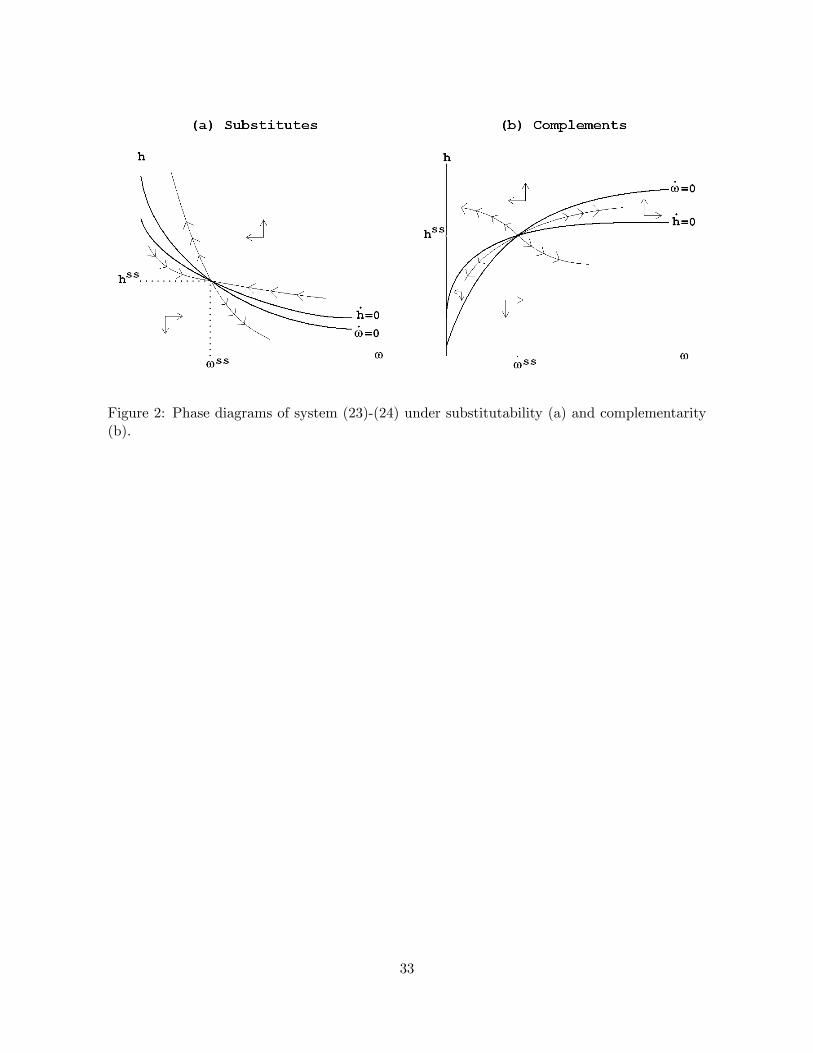
Figure 2: Phase diagrams of system (23)-(24) under substitutability (a) and complementarity(b).

33

Figure 3: Phase diagrams of system (23)-(24) in the Cobb-Douglas case for three di¤erentparametrizations.

34

Figure 4: Dynamics in the model with minimum resource requirement. Upper panel: thestationary locus h( _h=0) obtained from (43) under substitutability (a), complementarity (b) andCobb-Douglas (c) for increasing values of �. Lower panel: phase diagrams of system (42)-(43).

35