J Econ Growth (2015) 20:305–331DOI 10.1007/s10887-015-9118-z

Growth on a finite planet: resources, technology andpopulation in the long run

Pietro F. Peretto1 · Simone Valente2

Published online: 2 July 2015© Springer Science+Business Media New York 2015

Abstract We study the interactions between technological change, resource scarcity andpopulation dynamics in a Schumpeterian model with endogenous fertility. We find a steadystate in which population is constant and determined by resource scarcity while incomegrows exponentially. If labor and resources are substitutes in production, income and fertilitydynamics are stable and the steady state is the global attractor of the system. If labor andresources are complements, income and fertility dynamics are unstable and drive the economytowards either demographic explosion or collapse. We calibrate the model numerically tomatch past US data on fertility and land scarcity, obtaining future scenarios for the currentcentury and quantifying the response of fertility and productivity to exogenous shocks.

Keywords Endogenous innovation · Resource scarcity · Population growth · Fertilitychoices

JEL codes E10 · L16 · O31 · O40

1 Introduction

More than two centuries after the publication of Thomas Malthus’ (1798) Essay on thePrinciple of Population, understanding the interactions between economic growth, resourcescarcity and population remains a central aim of scholars in different fields of social sciences.

Electronic supplementary material The online version of this article (doi:10.1007/s10887-015-9118-z)contains supplementary material, which is available to authorized users.

B Pietro F. Perettoperetto@econ.duke.edu

Simone Valentes.valente@uea.ac.uk

1 Department of Economics, Duke University, Room 241, Durham, NC 27708, USA

2 School of Economics, University of East Anglia, ARTS 3.50, Norwich NR4 7TJ, UK

123

306 J Econ Growth (2015) 20:305–331

The debate revolves around two fundamental questions: (1) whether a larger population isgood or bad for human development and welfare (Birdsall and Sinding 2001; Kelley 2001)and (2) how population growth changes with economic conditions (Kremer 1993; Wanget al. 1994). There is an emerging consensus that both subjects should be tackled at the sametime: assessing the consequences of a growing population requires considering the feedbackeffects of resource scarcity on fertility (Bloom and Canning 2001). A prominent example isthe literature on unified growth theory (UGT), which seeks to explain the historical phasesof development, from the Malthusian Stagnation to the Industrial Revolution and then thecurrent regime of sustained growth of per capita incomes (Galor and Weil 2000; Galor 2005,2011). In the benchmark UGT model, the central mechanism behind economy-environmentinteractions is that population growth affects natural resource scarcity and labor productivity,while income dynamics affects fertility and thus future population growth.

In this paper, we investigate the mechanism linking resource scarcity, incomes and pop-ulation in a Schumpeterian model of endogenous growth. Our theory delivers an interactionbetween income dynamics and fertility but, differently from UGT, the feedback effect ofresource scarcity operates through resource prices and incomes, and may have oppositedirections depending on the degree of substitutability between labor and resources in theproduction of intermediate goods. In fact, our main results hinge on a ‘resource price effect’that is specific to our model, as we discuss below. Our general aim is to build a theory ofeconomy-environment interactions capable of addressing one of the main future challengesfor modern industrialized economies: how to sustain innovation-driven income per capitagrowth in a habitat—Planet Earth—that has finite carrying capacity of people. We tacklethis issue by studying under what circumstances population-resource dynamics generate asteady state where income per capita grows at a constant (endogenous) rate while populationstabilizes at a constant (endogenous) level.

In our model firms produce intermediate goods using labor and a resource in fixedaggregate supply—e.g., land—while households make fertility choices according to utilitymaximization. We employ a Schumpeterian model of endogenous growth in which horizon-tal and vertical innovations coexist: firms producing differentiated goods undertake R&Dto increase their total factor productivity while outside entrepreneurs design new productsand set up new firms in order to serve the market (Peretto 1998; Dinopoulos and Thompson1998). This class of models has received substantial empirical support in recent years (Lainczand Peretto 2006; Ha and Howitt 2007; Madsen 2008; Madsen et al. 2010; Madsen and Ang2011) and is particularly useful in addressing our research question because it predicts that theeffect of endowments on growth is only temporary. Specifically, product proliferation, i.e.,net entry, sterilizes the (strong) scale effect in steady state because it fragments the aggregatemarket into submarkets whose size does not increase with the size of the endowments. Inour analysis with endogenous fertility, the elimination of the (strong) scale effect generatessteady states in which population is constant and does not affect productivity growth.

Our first result is that there exists a steady state in which income per capita grows ata constant rate and population is constant. Importantly, the existence of this steady stateis not due to specific assumptions on fertility preferences but rather to the price effectsgenerated by the degree of substitutability between labor and resources in the production ofgoods: if we impose unit elasticity of input substitution, such steady state disappears andthe long-run growth rate of population is constant. Our second result is that the elasticityof substitution between labor and resources determines the stability properties of the steadystate. More precisely, if labor and resources are substitutes, the economy converges to thesteady state with constant population for any initial condition. The reason is that populationgrowth reduces the resource-labor ratio but, due to substitutability, the resource price rises

123

J Econ Growth (2015) 20:305–331 307

only moderately. As a consequence, resource income declines over time relative to laborincome, the fertility rate decreases and population stabilizes in the long run. If labor andresources are complements, instead, the steady state with constant population is a separatingthreshold: if the resource is either initially scarce or abundant, population diverges and wehave demographic explosion or collapse. The reason is that complementarity generates aself-reinforcing feedback effect: starting from the steady state, a rise in population yields aresource price increase that raises resource income, boosting fertility and thereby populationgrowth. If, instead, the deviation from the steady state is toward resource abundance—i.e., adrop in population—the resource price response induces lower income and further populationdecline.

We stress that feedback effects from resource income per capita to fertility decisions areneutralized in the special case of unit elasticity, i.e., when labor and resources are neithercomplements nor substitutes. This conclusion is relevant in three respects. First, it impliesthat departing from the hypothesis of Cobb–Douglas technology can be crucial for long-termpredictions on fertility and growth, whereas most related studies assume a unit elasticitybetween labor and fixed factors (e.g., Hansen and Prescott 2002; Lucas 2002; Doepke 2004).Second, the result is important from an empirical perspective since the recent cross-countryevidence rejects the hypothesis of unit elasticity between labor and land (or labor and naturalresources treated as fixed factors: see Ashraf et al. 2008; Weil and Wilde 2009). Third, ourprediction that constant long-run population growth rates only emerge in the Cobb–Douglascase captures a simple, yet often neglected idea: the hypothesis of exponential populationgrowth in the long run is clearly at odds with the fact that Planet Earth has a finite carryingcapacity of people.

We complete our analysis by presenting three applications of the model. First, we studythe fertility response to exogenous income shocks, stressing the consistency between ourqualitative results and recent evidence on the fertility–income relationship (Brückner andSchwandt 2014). Second, we calibrate the model to match the 1960–2012 data on birth ratesand land scarcity in the US, obtaining transitional dynamics that are consistent with the actualco-evolution of birth rates and income (Jones and Tertilt 2008). Third, using the in-samplecalibration, we construct a reference equilibrium path for the 1960–2100 period. This allowsus to use the US economy as a laboratory to quantify the potential consequences of a futuredemographic shock affecting the US from the year 2025 onwards.1

With respect to the existing literature on population-resource interactions, our analysisdiffers in both ends and means. In UGT models, consumption goods are produced by meansof human capital and land, population growth affects labor productivity, and the resultingincome dynamics determine fertility rates. Our analysis provides different insights for threemain reasons. First, UGT assigns a central role to human capital whereas our theory focuseson the fertility response to resource prices: the twomechanisms are notmutually exclusive andeach of them explains different stylized facts that characterized the 20th century.2 Second,both the nature and the role of technological change are different. In our model, verticalinnovations are Hicks-neutral with respect to labor and land so that technical change is

1 Given the lack of global data, using a specific country as a laboratory allows us to investigate the empiricaland quantitative properties of the model. We show in Sect. 6 below that our model can be applied to a singleeconomy with a minimum departure from the hypothesis of a closed system.2 More specifically, with respect to TFP growth our model predicts that fertility and TFP growth are pos-itively associated along the transition (both decline). Within our framework this outcome is consistent andintuitive: lower fertility slows down the growth of market size, which reduces the incentive for R&D. In UGT,instead, fertility and TFP growth are negatively correlated and productivity growth is driven by human capitalaccumulation, from which we abstract. We thank an anonymous referee for pointing this out.

123

308 J Econ Growth (2015) 20:305–331

consistent with constant population in the long run; in UGT, instead, technical change island-augmenting and lifts the economy out of the Malthusian trap by allowing population togrow when the subsistence consumption constraint is binding. Third, our main results hingeon a ‘resource price effect’ that is specific to our model: the response of fertility to increasedresource scarcity may be positive or negative, depending on the strength of the increasein the market resource price relative to the wage rate. Notably, the resource price effect isalso neglected in the parallel literature on industrial take-offs (e.g., Lucas 2002) because theexisting models either abstract from the resource market or, when they allow for a resourcemarket, assume a unit elasticity of substitution between labor and resources.3

Considering alternative approaches, there is an established literature on bio-economic sys-tems that seeks to explain the rise and fall of civilizations by modeling the relation betweenpopulation dynamics and resource availability in closed systems (e.g., islands) where naturalresources’ regeneration interacts with human harvesting. These models generate rich dynam-ics, including feast–famine oscillating paths and/or environmental crises that can eventuallydrive human society to extinction (Taylor 2009), and have been calibrated to replicate thecollapse of Easter Island and similar historical episodes (Brander and Taylor 1998; Basenerand Ross 2005; Good and Reuveny 2009). However, they neglect a fundamental element inthe functioning of modern societies: endogenous, innovation-driven productivity growth.

A strand of literature that comes close to our quest for more comprehensive predictionsfor future growth in a finite habitat is that on sustainable development, since it embraces aforward-looking perspective by definition (Pezzey 1992). At the conceptual level, sustain-ability analysis is motivated by the concern that future intergenerational conflicts will hingeon three issues: the scarcity of primary inputs, the environmental damage caused by economicactivity, and the further pressure exerted by population growth on both resource scarcity andenvironmental quality. Formal theories, however, insist on the first two issues—in particular,exhaustible resources (Smulders 2005) and pollution externalities (Xepapadeas 2005)—andtypically neglect the interdependence of scarcity and fertility. Despite its obvious relevancefor sustainability, only a few contributions formally analyze the fertility-scarcity interaction(Schäfer 2014; Bretschger 2013).4

2 The model

There are two main groups of agents. The first is a representative household who purchases ahomogeneous consumption good, supplies labor services and a natural resource (e.g., land)in competitive markets, accumulates wealth in the form of financial assets, and, crucially,makes reproduction decisions. The consumption good is produced by final firms assemblingdifferentiated intermediate inputs, each variety ofwhich is supplied by onemonopolistic firm.These intermediate firms are the second main group of actors in the model since productivitygrowth stems from their decisions concerning two types of innovations. First, the mass ofintermediate firms increases due to the costly development of new product lines (horizontalinnovation). Second, each intermediate firm undertakes in-house R&D to increase it own

3 A recent exception is Strulik and Weisdorf (2008), which investigates how the price of agricultural goods,determined in a two-sector economy by land scarcity and learning-by-doing activities, affects populationgrowth and economic growth.4 Schäfer (2014) builds a model of directed technological change in which skill-biased technological changeinduces a decline in population growth and a transitory increase in the depletion rate of natural resources.Bretschger (2013) considers poor substitution (complementarity) between labor and an exhaustible resourcein a Romer-style model of endogenous growth that exhibits the strong scale effect.

123

J Econ Growth (2015) 20:305–331 309

productivity (vertical innovation). The interplay between horizontal and vertical innovationsallows the economy to grow in steady state at a constant endogenous rate that is independentof factor endowments (Peretto 1998; Dinopoulos and Thompson 1998; Peretto and Con-nolly 2007). Connolly and Peretto (2003) studied the role of endogenous fertility in thisframework. Our analysis extends the model to include privately-owned natural resources andvarying degrees of substitutability between labor and resource inputs, exploiting the tractableframework developed by Peretto (2012).5

2.1 Households

The law of motion of adult population postulates that childhood lasts for one instant and thenthe child becomes an adult worker:

L (t) = B (t) − d · L (t) , (1)

where L is the mass of adults, B is the mass of children and d > 0 is the exogenous andconstant death rate. Children consume the same homogeneous good as adults but do notwork. Consumption and reproduction decisions are endogenous and reflect the intertemporalchoices of a single representative household who maximizes

U ≡∫ ∞

0log u(t)e−ρt dt, (2)

where u (t) is instantaneous utility at time t , and ρ > 0 is the discount rate. Instantaneousutility depends on consumption per adult, CL , consumption per child, CB , the mass of adultsand the mass of children, according to

log u (t) = μ log(CL (t) L (t)η

) + (1 − μ) log(CB (t) B (t)η

), (3)

where the parameters μ and η are both positive and below unity. This specification of pref-erences postulates that the decision maker cares about utility of adults and utility of childrenwith weights μ and 1− μ, and that each individual derives utility from own individual con-sumption as well as from the mass of individuals with weight η. The fact that CB is partof the decision problem introduces a trade-off in reproduction choices between the mass ofchildren and consumption expenditure per child.6 For future reference, we rewrite (3) as

log u (t) = logCL (t)μ CB (t)1−μ + log L (t)η + log b (t)η(1−μ) , (4)

where b (t) ≡ B (t) /L (t) is the gross fertility rate, and η (1 − μ) is the associated weightin household utility.

Each adult supplies inelastically one unit of labor to the production sector of the economy.The household is also endowed with� units of a non-exhaustible natural resource (e.g., land)that it supplies inelastically to manufacturing firms. The wealth constraint reads

A (t) = r (t) A (t) + w (t) L (t) + p (t) � − PC (t) [CL (t) L (t) + CB (t) B (t)] , (5)

5 Peretto (2012) studies the effects on income, growth andwelfare of a shock to the natural resource endowmentin a model with constant population.6 The original version of this paper (Peretto and Valente 2013) did not consider child consumption as anargument in the utility function. We thank an anonymous referee for suggesting this extension that producesthe same qualitative results but allows us to incorporate a quantity-quality tradeoff in the spirit of UnifiedGrowth Theory. Our results are nonetheless robust to alternative preference specifications as discussed inSect. 5.4.

123

310 J Econ Growth (2015) 20:305–331

where A is assets holding, r is the rate of return on assets, w is the wage rate, p is the marketprice of the resource and PC is the price of consumption. The household maximizes welfare(2) subject to the dynamic laws (1) and (5), using consumption and fertility levels as controlvariables and taking all prices as given.

2.2 Final sector

In the final sector, perfectly competitive firms produce the consumption good by means ofmanufactured intermediate inputs using the technology

C (t) =(∫ N (t)

0Xi (t)

ε−1ε di

) εε−1

, (6)

where C is total output of the homogeneous good, N is the mass of varieties of intermediateinputs, Xi is the quantity of the i-th variety, and ε > 1 is the elasticity of substitution betweenpairs of intermediate goods. Final producers maximize profits taking the prices and the massof varieties as given. The resulting demand for each intermediate good is

PXi (t) = PC (t) C (t)∫ N (t)0 Xi (t)

ε−1ε di

· Xi (t)−1ε , (7)

where PXi is the price of the i th variety.

2.3 Intermediate production and vertical innovation

Each variety of intermediate input is supplied by a monopolist. The intermediate firm ioperates the production technology

Xi (t) = Zi (t)θ · F(L Xi (t) − φ, Ri (t)

), (8)

where Xi is output, L Xi is overall labor employed in production, φ > 0 is a fixed operatingcost in units of labor (henceforth, fixed operating cost), Ri is the resource input, and F (·, ·) is astandardproduction functionhomogeneousof degreeone in itsmain arguments.7 Importantly,F (·, ·) may exhibit an elasticity of input substitution below or above unity. Whether laborand the resource are complements or substitutes matters for our results and we will discussall possible scenarios, including the case of unit elasticity where F (·, ·) is Cobb–Douglas.

The productivity of the firm depends on the stock of firm-specific knowledge, Zi , withelasticity θ ∈ (0, 1). Importantly, this firm-specific productivity term is Hicks-neutral withrespect to labor and the resource. The stock of firm-specific knowledge increases accordingto

Zi (t) = αK (t) L Zi (t) , (9)

where L Zi is labor employed in R&D. The productivity of labor in R&D depends on theexogenous parameter α > 0 and on the stock of public knowledge, K . Public knowledgeaccumulates as a result of spillovers across firms within the intermediate sector: when onefirm generates a new idea, it also generates non-excludable knowledge that benefits the R&D

7 The fixed operating cost, φ, ties product proliferation to population growth, as discussed in detail in Perettoand Connolly (2007). Section 4.2 clarifies how φ influences the interaction between the rates of horizontaland verical innovations.

123

J Econ Growth (2015) 20:305–331 311

of other firms according to the spillover function8

K (t) =∫ N (t)

0

1

N (t)Zi (t) di. (10)

Considering a monopolistic firm that starts to produce in instant t , the present discountedvalue of its net cash flow is

Vi (t) =∫ ∞

ti (v)e− ∫ v

t [r(v′)+δ]dv′dv, (11)

where i is the instantaneous profit, r is the instantaneous interest rate and δ > 0 is theinstantaneous death rate of firms.9 In each instant, the firm chooses the cost-minimizingcombination of rival inputs, L Xi and Ri , and the output level Xi that maximize static profitsi subject to the demand schedule (7) of final producers. Given this choice, the monopolistthen determines the time path of R&D employment L Zi that maximizes present-value profits(11) subject to the R&D technology (9), taking as given the other firms’ innovation paths.The solution to this problem is described in the Appendix and yields the maximized value ofthe firm given the time path of the mass of firms.

2.4 Horizontal innovation: entry

New firms enter the intermediate sector as time passes. Outside entrepreneurs hire labor toperform R&D activities that develop new varieties of intermediates, and then set up firms toserve the market. We assume that for each entrant, denoted i without loss of generality, thelabor requirement translates into a sunk entry cost (henceforth, entry cost) that is proportionalto the value of production of the new good when it enters the market, PXi Xi . Denoting byL Ni the labor employed in start-up activity, the entry cost is wL Ni = β PXi Xi , where β > 0is a parameter representing technological opportunity. This assumption captures the notionthat entry requires more effort the larger the anticipated volume of production.10

The value of the firm entering the market at time t equals the maximized present-valuenet cash flow Vi (t) because, once in the market, the firm solves an intertemporal problemidentical to that of the generic incumbent. Free entry, therefore, requires

Vi (t) = β PXi (t) Xi (t) = w (t) L Ni (t) (12)

for each entrant.

3 Equilibrium conditions

The intertemporal choices of households and the profit-maximizing behavior of firms charac-terize the equilibrium path of the economy. This section describes consumption and fertilitydecisions, the dynamics of innovation rates and the relevant market-clearing conditions.

8 Specification (10) is the simplest form of spillover function that eliminates the strong scale effect in modelsof this class, and exhibits sound microfoundations as discussed in Peretto and Smulders (2002).9 The main role of the instantaneous death rate is to avoid the asymmetric dynamics and associated hysteresiseffects that arise when entry entails a sunk cost. Such unnecessary complications would distract attention fromthe main point of the paper.10 Our assumption on the entry cost can be rationalized in several ways and does not affect the generality ofour results. Peretto and Connolly (2007), in particular, discuss alternative formulations of the entry cost thatyield the same qualitative properties for the equilibrium dynamics of the mass of firms that we exploit here.

123

312 J Econ Growth (2015) 20:305–331

3.1 Consumption and fertility choices

From (4), the Hamiltonian for the household problem takes the general form

H ≡ log u (CL , CB , L , b) + λA · A + λL · L,

where (CL , CB , b) are the control variables and λA and λL are the marginal shadow values ofasset holdings and household size, respectively. The necessary conditions for maximizationare derived in Appendix and yield three key relationships. The first is the standard Eulerequation

PC (t)

PC (t)+ C (t)

C (t)= r (t) − ρ (13)

which governs the dynamics of total consumption expenditure. The second relationship isthe static condition determining fertility choice at instant t ,

η (1 − μ) + λL (t) B (t) = 1 − μ, (14)

which equates the current utility value of generating children to the current utility cost ofproviding consumption to them.11 The third relationship is the dynamic law governing thegross fertility rate over time: by combining (14) with the relevant co-state equation for themarginal shadow value λL , we obtain

b (t)

b (t)= b (t)

(1 − μ) (1 − η)·[η + w (t) L (t) − PC (t) C (t)

PC (t) C (t)

]︸ ︷︷ ︸

Rate of return from generating future adults

− ρ. (15)

Expression (15) asserts that the fertility rate increases over time when the anticipated rate ofreturn from generating future adults exceeds the utility discount rate ρ. The term in squarebrackets in (15) emphasizes two components of this rate of return. The first is the elasticityparameter η, reflecting the direct utility benefit of expanding the future mass of adults. Thesecond component is a ‘private productivity gain’—namely, the anticipated net gain for thehousehold of generating a future worker –measured by the (rate of) excess of household laborincome, wL , over household consumption expenditures, PC C . The private productivity gainis the crucial channel whereby firms’ productivity and resource scarcity affect the dynamicsof the fertility rate in our model.

3.2 Production and innovation rates

In the intermediate sector, the solution to the typical firm’s problem yields a symmetricequilibrium: as shown in the Appendix, each monopolist charges the same price PXi = PX

and produces the same quantity of intermediate good, Xi = X . Combining this result withthe zero-profit condition in the final sector, the total value of intermediates equals totalconsumption expenditure, with each monopolist capturing the same share 1/N of the goods’total market value:

PX (t) X (t) = PC (t) C (t)

N (t). (16)

11 In the left hand side of (14), the current utility value to the household of generating children representedby direct utility benefits (from (4), the term η (1 − μ) is the elasticity of utility to the fertility rate) plus theshadow value of increasing current population, λL B. The right hand side of Eq. (14) is the current utility cost,represented by the elasticity of utility to child consumption, 1 − μ.

123

J Econ Growth (2015) 20:305–331 313

Accordingly, the output quantities of the final and the intermediate sectors are linked throughthe equilibrium relationship

C (t) = N (t)ε

ε−1 X (t) . (17)

Considering employment in the intermediate sector, we can write the aggregate quantitiesof labor employed in production and vertical R&D as L X = N L Xi and L Z = N L Zi ,respectively. Similarly, total resource use in manufacturing production equals R = N Ri .The typical firm’s knowledge stock is Zi = Z for each i ∈ [0, N ] and evolves according to

Z (t)

Z (t)= α

L Z (t)

N (t). (18)

Since the value of an intermediate firm’s production is PX X = PC C/N , the free-entrycondition (12) implies Vi N = β PC C . Using this result, and denoting total employment instart-up operations by L N = (N + δN ) · L Ni , the net increase in the mass of firms equals

N (t)

N (t)= w (t)

β PC (t) C (t)· L N (t) − δ. (19)

The rates of vertical and horizontal innovation in (18) and (19) are interdependent throughthe no-arbitrage condition that the associated returns must be equal (see Appendix).

3.3 Market clearing conditions

Reseource market clearing requires that total resource use in intermediates production, R =N Ri , be equal to the available endowment: R = �. Accordingly, the household’s resourceincome equals p�.

Labor market clearing requires L = L X + L Z + L N . Asset market equilibrium requiresthat the value of the household’s portfolio equal the value of the securities issued by firms:A = N Vi = β PC C . Substituting this condition into the wealth constraint (5), and using thesaving rule (13), we obtain

PC (t) C (t) = 1

1 − βρ[w (t) L (t) + p (t)�] . (20)

This expression says that the ratio of household consumption expenditure to the household’sincome from labor and land, wL + p�, is constant over time.

4 General equilibrium dynamics

For clarity, we split the analysis of dynamics in two parts. First, we study the interactionof population and resource scarcity (Sect. 4.1). Next, we describe the interaction betweenhorizontal and vertical innovations in determining productivity growth (Sect. 4.2). A crucialcharacteristic of the resulting dynamics is the existence of a steady state displaying constantpopulation associated to constant growth of (real) consumption per capita. Henceforth, wetake labor as the numeraire and set w (t) ≡ 1 in each instant t . This normalization implies,inter alia, that an increase in p represents an increase in the resource price relative to thewage rate.

123

314 J Econ Growth (2015) 20:305–331

4.1 Fertility and resource scarcity

In this subsectionwe characterize the interactions betweenpopulation and resource scarcity asa dynamic system involving two variables: the resource endowment per capita and the fertilityrate. The resource endowment per capita, ω (t) ≡ �/L (t), is a state variable that is givenat time zero but is subsequently driven by fertility choices via the dynamics of population.We derive the dynamical system in two steps. In Sect. 4.1.1, we treat the value of ω (t)as given at time t and derive the equilibrium values of the resource price and consumptionexpenditure per capita. Building on this result, in Sect. 4.1.2 we derive the two-by-two systemthat describes the joint dynamics of ω (t) and b (t).

4.1.1 Fertility, expenditure and resource price

Denoting consumption expenditure per capita by y ≡ PC C/L , the equilibrium condition(20) becomes

y (t) = 1 + p (t) ω (t)

1 − βρ, (21)

which says that consumption expenditure per capita is proportional to the sumof labor incomeper capita, 1, and resource income per capita, p (t) ω (t). Resource income per capita, inturn, is determined by the equilibrium between the demand for the resource by firms andthe household’s supply. From the firms’ conditional demand for the resource, we obtain (seeAppendix)

p (t) ω (t) = ε − 1

ε· S (p (t)) · y (t) , (22)

where S (p) ∈ (0, 1) is the cost share of resource use—i.e., the ratio between totalresource rents paid by firms to resource owners and the total variable costs of manufac-turing production—and is a function of the resource price. This expression specifies howexpenditure decisions determine resource income through the endogenous resource price.Specifically, the cost share of resource use S (p) is increasing or decreasing in the resourceprice depending on the elasticity of input substitution (see Appendix):

∂S (p)

∂p

⎧⎨⎩

> 0 if(L Xi , Ri

)are complements;

< 0 if(L Xi , Ri

)are substitutes;

= 0 if F (·, ·) is Cobb–Douglas.(23)

The intuition for result (23) is that, under complementarity (substitutability), the resourcedemand per unit of labor is relatively rigid (elastic) and an increase in the resource priceraises (reduces) the share of firm’s costs for resource use relative to wage payments. Thiscost-share effect plays a crucial role in our results.

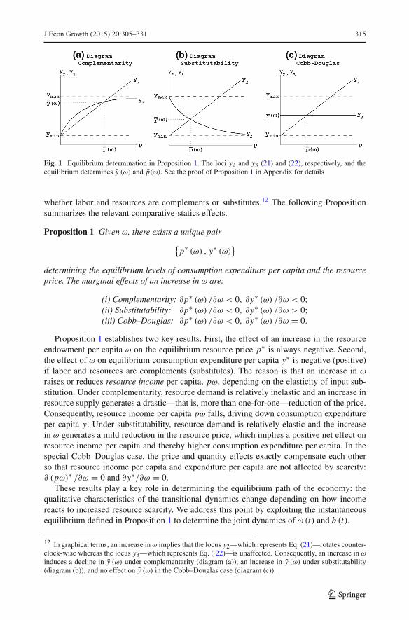
For a given level of the resource endowment per capita, ω (t), Eqs. (21) and (22) forma static system in two unknowns that determines the equilibrium levels of p (t) and y (t).Figure 1 describes graphically the equilibrium determination, showing that that equilibriumexpenditure per capita always falls within the interval y (ω) ∈ (ymin, ymax), where ymin =

11−ρβ

and ymax = 1(1/ε)−ρβ

(see Appendix). Importantly, consumption expenditure per capitaresponds differently to variations in the resource endowment per capita ω (t) depending on

123

J Econ Growth (2015) 20:305–331 315

Fig. 1 Equilibrium determination in Proposition 1. The loci y2 and y3 (21) and (22), respectively, and theequilibrium determines y (ω) and p(ω). See the proof of Proposition 1 in Appendix for details

whether labor and resources are complements or substitutes.12 The following Propositionsummarizes the relevant comparative-statics effects.

Proposition 1 Given ω, there exists a unique pair{

p∗ (ω) , y∗ (ω)}

determining the equilibrium levels of consumption expenditure per capita and the resourceprice. The marginal effects of an increase in ω are:

(i) Complementarity: ∂p∗ (ω) /∂ω < 0, ∂y∗ (ω) /∂ω < 0;(ii) Substitutability: ∂p∗ (ω) /∂ω < 0, ∂y∗ (ω) /∂ω > 0;(iii) Cobb–Douglas: ∂p∗ (ω) /∂ω < 0, ∂y∗ (ω) /∂ω = 0.

Proposition 1 establishes two key results. First, the effect of an increase in the resourceendowment per capita ω on the equilibrium resource price p∗ is always negative. Second,the effect of ω on equilibrium consumption expenditure per capita y∗ is negative (positive)if labor and resources are complements (substitutes). The reason is that an increase in ω

raises or reduces resource income per capita, pω, depending on the elasticity of input sub-stitution. Under complementarity, resource demand is relatively inelastic and an increase inresource supply generates a drastic—that is, more than one-for-one—reduction of the price.Consequently, resource income per capita pω falls, driving down consumption expenditureper capita y. Under substitutability, resource demand is relatively elastic and the increasein ω generates a mild reduction in the resource price, which implies a positive net effect onresource income per capita and thereby higher consumption expenditure per capita. In thespecial Cobb–Douglas case, the price and quantity effects exactly compensate each otherso that resource income per capita and expenditure per capita are not affected by scarcity:∂ (pω)∗ /∂ω = 0 and ∂y∗/∂ω = 0.

These results play a key role in determining the equilibrium path of the economy: thequalitative characteristics of the transitional dynamics change depending on how incomereacts to increased resource scarcity. We address this point by exploiting the instantaneousequilibrium defined in Proposition 1 to determine the joint dynamics of ω (t) and b (t).

12 In graphical terms, an increase in ω implies that the locus y2—which represents Eq. (21)—rotates counter-clock-wise whereas the locus y3—which represents Eq. ( 22)—is unaffected. Consequently, an increase in ω

induces a decline in y (ω) under complementarity (diagram (a)), an increase in y (ω) under substitutability(diagram (b)), and no effect on y (ω) in the Cobb–Douglas case (diagram (c)).

123

316 J Econ Growth (2015) 20:305–331

4.1.2 Dynamic system

Since the total resource endowment is fixed, resources per capita decline as population grows:from (1), the dynamics of ω (t) obey the differential equation

ω (t) = ω (t) · (d − b (t)) . (24)

The dynamics of the fertility rate are governed by Eq. (15): the marginal return from gener-ating future workers may be re-expressed in terms of expenditure per capita as

b (t)

b (t)=

[1

(1 − η) · y∗ (ω (t))− 1

]· b (t)

1 − μ− ρ, (25)

where the properties of the equilibrium relationship y∗ (ω) are those established in Propo-sition 1. The system formed by (24) and (25) allows us to analyze the general equilibriumdynamics of the resource-population ratio and the fertility rate. Before studying in detail theproperties of this system, we complete the description of the general equilibrium dynamicsby considering innovation rates and productivity growth.

4.2 Innovations and productivity growth

In this model real final output is equal to real consumption. Accordingly, the growth rate ofthe economy, G (t), is (see Appendix)

G (t) ={θ · Z (t)

Z (t)+ 1

ε − 1· N (t)

N (t)

}︸ ︷︷ ︸

TFP growth rate

+[

y (t)

y (t)− S (p (t)) · p (t)

p (t)

]︸ ︷︷ ︸Transitional resource-income effect

, (26)

where the term in curly brackets represents the growth rate of total factor productivity (TFP)determined by vertical and horizontal innovations. The ‘transitional resource-income effect’in square brackets, instead, captures possible unbalanced dynamics among expendituresper capita, resource price and the wage rate. If the economy reaches a balanced growthequilibrium where both expenditure per capita and the resource price are proportional tothe wage rate (normalized to unity), we have y (t) = p (t) = 0 and the term in squarebrackets becomes zero. Out of such steady states, however, the contribution of the transitionaldynamics of resource income to the overall real growth rate can be substantial. Moreover,we can distinguish between a first component, y/y, which captures the role of expendituregrowth in raising resource demand, and a second component, S (p) · p/p, which representsthe scarcity drag, i.e., the increase in the resource price due to the growing resource demand.We study the quantitative importance of these components in Sect. 6 below.

The costly development of vertical andhorizontal innovations is profitable only if thefirm’svolume of production is large enough: there thus exist thresholds of market size below whichvertical innovation or horizontal innovation, or both, are inactive because firms cannot obtaina rate of return equal to the prevailing interest rate in the economy. These thresholds, whichwediscuss in theAppendix13, play an important role in the characterization of early developmentphases—where “no-innovation traps” plausibly arise—but have no crucial bearing on thepresent analysis,which focuses on the future behavior of an economy that has already transitedto “modern” production. Consequently, we henceforth assume that the values of the relevant

13 The proof of Lemma 2 in Appendix proves the existence of threshold levels in firm size determining regionsof the phase space where vertical and/or horizontal innovations shut down.

123

J Econ Growth (2015) 20:305–331 317

parameters and the initial conditions (L (0) , N (0)) are such that both vertical and horizontalinnovations are active.

The following Lemma establishes that, in equilibrium, the rates of vertical and horizontalinnovation are jointly determined by two variables: firm size, denoted by x ≡ PX X =PC C/N , and the interest rate.

Lemma 2 Along the equilibrium path, the rates of vertical and horizontal innovation are,respectively:

Z (t)

Z (t)= x (t) · αθ (ε − 1)

ε− r (t) − δ, (27)

N (t)

N (t)= 1

β

[1 − θ (ε − 1)

ε− 1

x (t)·(

φ − r (t) + δ

α

)]− ρ − δ. (28)

The behavior of firm size, x (t), is governed by the differential equation

x (t) = αφ − r (t) − δ

αβ− 1 − θ (ε − 1) − βε (r (t) + δ)

βε· x (t) . (29)

According to Eq. (29), the evolution of firm size depends on the equilibrium path of theinterest rate. The interest rate, in turn, follows the dynamics of aggregate market size, thatreflect households’ consumption and fertility choices: from (1) and (13), we have

r (t) = ρ + y (t)

y (t)+ b (t) − d. (30)

These results highlight the functioning of the modern economy captured by our model struc-ture: the path of the interest rate carries all the information that firms need in order to choosepaths of vertical and horizontal R&D that are consistent with the evolution of the size of themarket for manufacturing goods. The path of market size, in turn, depends on the evolutionof the economy’s resource base, that is, on the path of population.

Before analyzing population dynamics, we characterize the behavior of productivitygrowth when the economy converges to a steady state where expenditure per capita, popula-tion and the resource price are constant. Eqs. (26) and (30) imply that in such a steady state,the interest rate equals r (t) = ρ and the economy’s real growth rate equals the TFP growthrate. Then, the following result holds:

Proposition 3 Suppose that limt→∞ y (t) = limt→∞ p (t) = limt→∞ L (t) = 0. Then, thenet rate of horizontal innovation is zero and income growth is exclusively driven by verticalinnovation:

limt→∞

N (t)

N (t)= 0 and lim

t→∞ G (t) = θ · limt→∞

Z (t)

Z (t). (31)

Provided that parameters satisfy ρ + δ <αφθ(ε−1)1−βε(ρ+δ)

, the growth rate is strictly positive:

limt→∞ G (t) = θ

θ (ε − 1) [αφ − (ρ + δ)]

1 − θ (ε − 1) − βε (ρ + δ)− θ (ρ + δ) > 0. (32)

Proposition 3 establishes twomain results concerning equilibria with constant population.First, as discussed in detail in Peretto (1998) and Peretto and Connolly (2007), steady-stateeconomic growth is exclusively driven by vertical innovation: the process of entry enlargesthe mass of goods until the gross entry rate matches the firms’ death rate. Consequently,the mass of firms is constant and each firm invests a constant amount of labor in verticalR&D. The second result is that steady-state real income growth is independent of factor

123

318 J Econ Growth (2015) 20:305–331

endowments because net entry eliminates the strong scale effect. This property allows theeconomy to exhibit equilibria in which population is constant but real income per capitagrows at a constant, endogenous rate. The next section addresses this point in detail.

5 Population, resources and technology

This section characterizes the equilibrium path of population and derives the main resultsof this paper. Population dynamics determine the supply of labor and the extent of resourcescarcity at each point in time.An important property of themodel is that the path of populationcan be studied in isolation from market size and innovation rates: system (24) and (25) fullycaptures the interactions between fertility and resource scarcity, and generates the equilibriumpaths of population and resource use underlying the dynamics of aggregatemarket size. Then,as explained in Sect. 4.2, aggregate market size and the interest rate induced by populationdynamics determine the evolution of firmsize and, ultimately, total factor productivity growth.

The next subsection studies the joint dynamics of fertility and resource endowment percapita, characterizing the steady state with constant population. The stability properties of thesteady state crucially depend on the elasticity of substitution between labor and the naturalresource in manufacturing production: Sect. 5.2 discusses strict complementarity and strictsusbstitutability, whereas Sect. 5.3 considers the special Cobb–Douglas case.

5.1 Steady state with constant population

Consider a steady state (ωss, bss) in which both the resource per capita and the fertility rateare constant. Imposing ω = 0 and b = 0 in the dynamic system (24 ) and (25), we obtain:

bss = d, (33)

bss = ρ (1 − μ)(1 − η) · yss (ωss)

1 − (1 − η) · yss (ωss). (34)

Equation (33) is the obvious requirement of zero net fertility for constant population. Equation(34) determines steady-state endwoment per capita ωss and thereby defines the stationaryvalue of expenditure per capita yss that is consistentwith the fertility rate bss = d . Concerningthe existence of a steady state with positive fertility rate bss > 0, it can be shown that η > ρβ

guarantees (1 − η) · yss < 1 and, hence, a positive right hand side in (34). In the remainderof the analysis, we impose this sufficient, though not necessary, parameter restriction.14

From Proposition 1, the steady-state equilibrium (ωss, bss) also implies a stationary valuefor the resource price, which we denote by pss . Concerning expenditure and populationlevels, we have:

14 The proof of Proposition 1 (see Appendix) shows that equilibrium expenditure per capita is always boundedby y (ω) ∈ (ymin, ymax), where ymin = 1

1−ρβand ymax = 1

(1/ε)−ρβ. Consequently, to guarantee that the

term in brackets is always positive it is sufficient to assume 11−η

> ymax, which necessarily holds as long asη > ρβ. It is possible to consider alternative cases where η � ρβ but this would complicate the phase-diagramanalysis without much gain in terms of economic insight.

123

J Econ Growth (2015) 20:305–331 319

Proposition 4 Assume η > ρβ. Then, there exists a steady state where expenditure percapita and population are, respectively:

yss = 1

1 − η· d

d + ρ (1 − μ)> 0, (35)

Lss = pss

yss · (1 − βρ) − 1· � > 0. (36)

Recall that by Proposition 3, given the constant values (pss, yss, bss), real income growthequals the constant rate of vertical innovation. An important characteristic of this steadystate is that yss and Lss are independent of technology. From (35), expenditure per capitadepends solely on preferences and demographic parameters: neither the endowment of thenatural resource, �, nor total factor productivity play any role. From (36), population isproportional to the resource endowment but remains independent of technology, while realincome per capita grows at the endogenous rate (32). Therefore, we have a steady state withthe property that resource scarcity limits the population level, but where real income growsat an endogenous rate driven by technological change. Before pursuing this property further,we need to assess whether and under what circumstances the economy converges to suchsteady state.

5.2 Dynamics under substitutability and complementarity

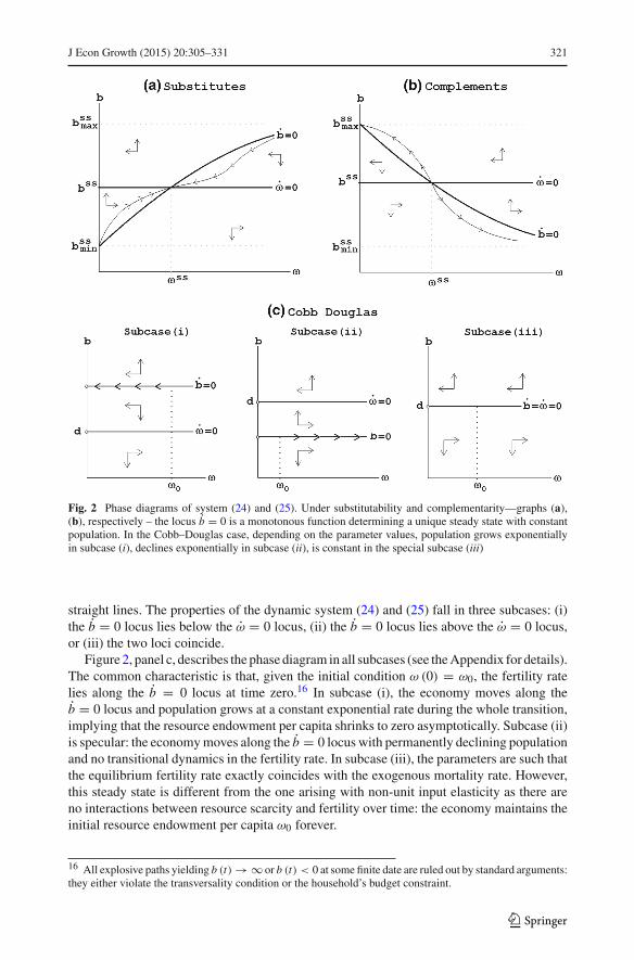
The stability of the steady state with constant population depends on the input elasticityof substitution in the intermediate sector. We thus have three main cases: complementarity,substitutability and unit elasticity (Cobb–Douglas). In this subsection we concentrate onstrict complementarity and strict substitutability. The phase diagrams for these cases, shownin Fig. 2, yield the following result.

Proposition 5 Under substitutability, the b = 0 locus is increasing and cuts the ω = 0 locusfrom below so that (ωss, bss) is saddle-path stable. Consequently, the steady state with con-stant population is the global attractor of the system. Under complementarity, the b = 0locus is decreasing and cuts the ω = 0 locus from above so that (ωss, bss) is an unstablenode or focus. Consequently, the steady state with constant population is a separating thresh-old: if the resource is initially scarce (abundant) relative to labor, the economy experiencesdemographic explosion (collapse).

Proposition 5 establishes that the economy converges to the steady state with constantpopulation if labor and the resource are substitutes in production. Under complementarity,instead, such steady state is unstable and the economy follows diverging equilibrium pathsleading to population explosion or collapse depending on the relative scarcity of the resourceat time zero.15

The intuition for these results follows from the effects of resource scarcity on resourceincome per capita established in Proposition 1. First, consider the case of substitutability:the equilibrium trajectory lies along the saddle path depicted in Fig. 2, diagram (a). Supposethat the resource is initially abundant, that is, ω0 > ωss . The initial equilibrium level of thefertility rate b (0) lying along the stable arm of the saddle exceeds the death rate d = bss

15 We report the details on the uniqueness of the equilibrium path in Appendix. For brevity, we focus onthe case in which the steady-state loci intersect and the steady state exists. Nonetheless, global dynamics arewell defined and the equilibrium path is unique even when the loci do not intersect: in such cases (which areessentially slight extensions of the Cobb–Douglas scenarios studied in Sect. 5.3) the system converges eitherto exponential population growth or to population collapse, depending on the parameters.

123

320 J Econ Growth (2015) 20:305–331

so that population grows and ω declines. As resources per capita shrink, the resource price,p, rises during the transition. Crucially, when labor and resources are substitutes, the priceeffect due to increasing land scarcity is not very strong and the economy experiences fallingresource income per capita, pω, and, consequently, a falling fertility rate (cf. Proposition1). Symmetrically, if the resource is relatively scarce at time zero, ω0 < ωss , net fertility isinitially negative, population shrinks during the transition and ω rises while p falls; since theprice effect is weak, resource income per capita pω rises, driving the fertility rate up. In bothcases, the transition ends when the fertility rate equals the death rate, d = bss . Hence, undersubstitutability the steady state with constant population is the global attractor of the systembecause population growth generates resource income dynamics that yield self-balancingfeedback effects: as resource scarcity tightens, the resource price rises, but less than one forone with the endowment, so that resource income per capita falls.

Now consider the case of complementarity in Fig. 2, diagram (b). In this scenario, thesteady state is not stable because the resource income effect is reversed. If the resource isinitially scarce, ω0 < ωss , the dynamics exacerbate scarcity because, as population growthreduces ω, the resource price p rises more than one for one yielding a rise of resourceincome per capita pω and a rise in fertility (cf. Proposition 1). This implies a feedbackeffect whereby population grows faster and drives the economy further away from the steadystate. Resource per capita ω then tends asymptotically to zero as the economy experiencesa demographic explosion. Symmetrically, if the resource is relatively abundant at time zero,ω0 > ωss , population shrinks and the increase in ω reduces resource income per capita viastrong reductions in the resource price p, yielding a negative effect on fertility. Hence, undercomplementarity, the steady state is not the global attractor of the system because populationgrowth generates resource income dynamics that yield self-reinforcing feedback effects onfertility.

The mechanism generating extinction under complementarity is quite different from thatsuggested by bio-economic models in which collapse is due to over-exploitation of the nat-ural resource base—see, e.g., D’Alessandro (2007) and, especially, Taylor (2009). In contrastto these stories, the demographic collapse in our model is due to an excessive scarcity ofmanpower that prevents the economy from taking advantage of the natural resource base.This situation is self-reinforcing because the low resource income per capita yields below-replacement fertility and further population decline. Moreover, as we highlighted in thediscussion of the dynamics of the innovation rates, the collapse of the population eventu-ally results in the shutting down of R&D activity and ultimately of modern manufacturingproduction itself.

Also, our results are novel with respect to those of Unified Growth Theory because thequalitative dynamics described in Fig. 2 are generated by a price effect that does not ariseif there is no resource market—as in Galor and Weil (2000)—or, if there is, when labor andresources exhibit a unit elasticity of substitution, as in Lucas (2002). To make this pointtransparent, we now turn to the Cobb–Douglas case and show that the steady state withconstant population is indeed created by the resource price effect.

5.3 The special Cobb–Douglas case

When the intermediate sector’s technology takes the Cobb–Douglas form, the steady statewith constant population does not exist and the model predicts that population grows orshrinks forever at a constant rate. The proof follows from Proposition 1. A unit elasticityof input substitution implies that neither expenditures nor the fertility rate are affected byvariations in resources per capita. Consequently, the ω = 0 and b = 0 loci become horizontal

123

J Econ Growth (2015) 20:305–331 321

Fig. 2 Phase diagrams of system (24) and (25). Under substitutability and complementarity—graphs (a),(b), respectively – the locus b = 0 is a monotonous function determining a unique steady state with constantpopulation. In the Cobb–Douglas case, depending on the parameter values, population grows exponentiallyin subcase (i), declines exponentially in subcase (ii), is constant in the special subcase (iii)

straight lines. The properties of the dynamic system (24) and (25) fall in three subcases: (i)the b = 0 locus lies below the ω = 0 locus, (ii) the b = 0 locus lies above the ω = 0 locus,or (iii) the two loci coincide.

Figure 2, panel c, describes the phase diagram in all subcases (see theAppendix for details).The common characteristic is that, given the initial condition ω (0) = ω0, the fertility ratelies along the b = 0 locus at time zero.16 In subcase (i), the economy moves along theb = 0 locus and population grows at a constant exponential rate during the whole transition,implying that the resource endowment per capita shrinks to zero asymptotically. Subcase (ii)is specular: the economymoves along the b = 0 locus with permanently declining populationand no transitional dynamics in the fertility rate. In subcase (iii), the parameters are such thatthe equilibrium fertility rate exactly coincides with the exogenous mortality rate. However,this steady state is different from the one arising with non-unit input elasticity as there areno interactions between resource scarcity and fertility over time: the economy maintains theinitial resource endowment per capita ω0 forever.

16 All explosive paths yielding b (t) → ∞ or b (t) < 0 at some finite date are ruled out by standard arguments:they either violate the transversality condition or the household’s budget constraint.

123

322 J Econ Growth (2015) 20:305–331

5.4 Remarks

5.4.1 Robustness

Our main results concerning the existence and stability properties of the steady state withconstant population are robust to alternative specifications of fertility preferences. In thecurrent analysis, the cost of child bearing cost is determined by the assumed trade-off betweenconsumption per adult and consumption per child. The original version of this paper (Perettoand Valente 2013) obtains the same predictions by assuming, instead, that child bearingentails a fixed time cost of reproduction which reduces total labor supply and thereby thehousehold labor income. More generally, the model predictions do not hinge on the natureof child bearing costs but rather on the fact that the response of fertility to increased resourcescarcity is determined by variations in resouce income per capita. For example, the ‘resourceprice mechanism’ driving the results would not arise in the absence of a resource market witheffective property rights.

5.4.2 Constant long-run population under complementarity

In the previous analysis, the economy permanently diverges from the steady state with con-stant population if labor and resources are complements. However, minimal extensions ofthe model may generate constant long-run population even under complementarity. In theoriginal version of this paper (Peretto and Valente 2013), for example, we assume that afraction of the per capita endowment of the resource cannot be exploited for productionpurposes—e.g., part of the economy’s total land must be devoted to residential use. Theexistence of a minimum resource requirement allows the economy to avoid demographicexplosion even under complementarity. The reason is that, as the resource per capita movesclose to the minimum threshold level, the land price signals congestion and fertility rates aresubject to an enhanced preventive check that always stabilizes the population level before itgrows too large. Moreover, this mechanism also operates with Cobb–Douglas technology,implying that the standard result of exponential population growth is a rather special case.

5.4.3 Technological change

Weassumed that the technological changedriving long-rungrowth—i.e., vertical innovations—is Hicks-neutral with respect to labor and land. It is possible to introduce land-augmentingtechnological change, as in UGT, but doing so would complicate the model without addinginsight to this paper’s research question. Since we focus on the future prospects for economicgrowth, we do not need to postulate a bias of technological change which may instead berelevant to study, e.g., the industrial take-off or the escape from a Malthusian trap.

5.4.4 Related empirical evidence

Our emphasis on the cases of complementarity and substitutability seems relevant froman empirical perspective since recent cross-country evidence rejects the hypothesis of unitelasticity between labor and land (or between labor and natural resources interpreted asfixed factors: see Ashraf et al. 2008; Weil and Wilde 2009). In particular, most contributionsfind high estimated values for the elasticity of substitution—e.g., Weil and Wilde (2009)report estimates ranging from 1.6 to 8.0. Concerning the joint dynamics of population and

123

J Econ Growth (2015) 20:305–331 323

income, however, there is no empirical work that attempts at testing the impulse-responsemechanism between fertility and resource income that characterizes our model.17 A recentstudy that points in a similar direction is Brückner and Schwandt (2014): although theiranalysis abstracts from feedback effects induced by the elasticity of substitution, they showthat positive income shocks raise population growth via increased fertility.We explain furtherthe link between our theory and Brückner and Schwandt’s (2014) empirical findings Sect. 6.1below.

6 Exogenous shocks and quantitative analysis

This section presents three applications of our model. First, we study the fertility responseto exogenous income shocks (Sect. 6.1), showing that the core mechanism of our theory isconsistent with recent evidence on the fertility-income relationship (Brückner and Schwandt2014). Second, in order to check the plausibility of the theoretical predictions, we applythe model to the United States by calibrating the parameters to match the 1960–2012 dataon birth rates and land scarcity (Sect. 6.2). In this exercise, we use the US economy asa laboratory: the simulation yields a reference future equilibrium path for the 1960–2100period, using the parameters of the in-sample calibration for 1960–2012. This applicationof the model to a single economy only requires a minimal departure from the hypothe-sis of a perfectly closed system. Third, we extend the benchmark simulation for the USto study, both qualitatively and quantitatively, the consequences of a demographic shock(Sect. 6.3).

6.1 Fertility response to income shocks

In a recent paper, Brückner and Schwandt (2014) document the fertility effects of incomeshocks using state-of-the-art dynamic panels for a large number of countries. Importantly,they use shocks to the world oil price as an instrument in the identification procedure,obtaining the result—crucial for our purposes—that positive exogenous income shocks raisepopulation growth via increased fertility. While Brückner and Schwandt (2014) do not spec-ify a theoretical model, their empirical result appears to address the core mechanism ofour model, i.e., the fertility response to income variations for given values of the funda-mental demographic parameters. We illustrate how by considering a parameter shock thatmodifies the steady state land-to-population ratio exclusively through the resource incomechannel.

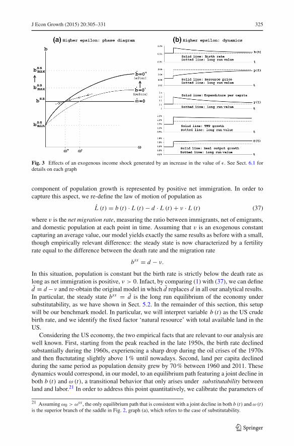
Suppose that labor and land are substitutes. The economy is initially in the steady statewith constant population, and there is a permanent unexpected rise in ε. Recalling expression(22), this shock produces a ceteris paribus increase in the amount of resource income. In thephase diagram of system (24) and (25), the shock implies a counter-clockwise rotation of theb = 0 locus whereas the ω = 0 locus is unchanged.18 As shown in Fig. 3, diagram (a), theshock yields a new steady state in which the long-run fertility rate bss is the same as before

17 This is partly due to lack of data on land rents for many countries, including the most developed economies.The same problem of data availability constrains the methods for estimating the elasticity of substitution (seeWeil and Wilde 2009).18 Formally, the reason for the shift is that a higher ε raises bss

max, i.e., the horizontal aymptote of the b = 0locus. In economic terms, variations in the parameters governing resource demand change resource income andthereby the opportunity cost of fertility—which means modifying the b = 0 locus—while the same variationsleave the natural law of resource depletion (24) unaffected.

123

324 J Econ Growth (2015) 20:305–331

but the long-run level of land per capita ωss is lower (ω′′ < ω′). The intuition is that thepositive income shock lowers the opportunity cost of fertility and initially drives the currentbirth rate above replacement. In the long run, instead, population is stabilized again as theprice effect generated by the increased scarcity offsets the net private gains from populationexpansion.

The sequence of events triggered by the shock is as follows. First, given ω, the positiveshock to resource demand yields a higher resource price p. Second, the resulting upwardjump in resource income raises expenditure per capita y. Third, the fertility rate b initiallyreacts to the higher expenditure with an upward jump on the saddle path leading to the newsteady state. Fourth, higher expenditure and slower population growth increase firm size,inducing entry of new firms as well as more vertical R&D investment by existing firms: thehigher rates of horizontal and vertical innovations raise TFP growth both in the short and insteady state.

Following the same logical order, the graphs reported in Fig. 3, panel b, provide a quantita-tive assessment of both the initial and the transitional effects of the income shock. We obtainthese diagrams assuming an initial steady statewith ε = 2.20 and a shock to ε = 2.46 . All theother parameter values are the same as in the calibration that we discuss in the next subsection.

Beyond its illustrative purpose, the numerical exercise delivers an additional result. Underthe assumed parameters, the growth rates of TFP and real output converge to the new steadystate level following qualitatively different transitional paths. Specifically, after the initialjumps, TFP growth declines monotonically whereas real output growth exhibits a hump-shaped path—i.e., it keeps on increasing for a while after the shock, reaches a peak andthen converges from above to the long-run level.19 Driving this difference is the behaviorof the transitional resource-income effect, see Eq. (26), which is strictly negative duringthe transition because we have y/y < 0 and p/p > 0. This effect becomes smaller andsmaller in absolute value as time passes, as y and p approach the respective steady states.In our calibration, this effect dominates the transitional TFP slowdown in the short-mediumrun, determining the hump-shaped path of real income growth. We will encounter a similareffect in the next subsection, where we apply the model to the US economy and interpretthis mechanism as a “resource-income drag” linked to the transitional decline of populationgrowth.

6.2 Birth rates and land scarcity in US

This subsection performs a numerical simulation of the model to study the joint dynamicsof birth rates and land scarcity in the United States. As a first step, we introduce a minormodification to the theorywhich allows us to reinterpret themodel as one of a single economythat is subject to migratory inflows. We then calibrate the model to match the 1960–2012data on birth rates and land scarcity in the US, obtaining a reference future equilibrium pathfor the whole present century.

Like in other industrialized economies, the age-adjusted fertility rate in the US is alreadybelow the replacement level20: total births are only slightly above total deaths, and a relevant

19 In Fig. 3, panel b, the pre-shock growth rate of both TFP and real output is 1.45% and the new long-rungrowth rate, represented by the dotted lines, is 1.83%. The last graph shows that G (t) reaches a peak above2% and then converges to 1.83% only in the very long run: the convergence speed of real output growth israther slow relative to the other variables, which makes the hump-shaped transitional path difficult to show inFig. 3, panel b.20 According to World Bank (2014) data, in each year within the 2011–2013 period, the average fertility ratein the US is 1.9 children per woman, strictly below the replacement ratio of 2.1.

123

J Econ Growth (2015) 20:305–331 325

Fig. 3 Effects of an exogenous income shock generated by an increase in the value of ε. See Sect. 6.1 fordetails on each graph

component of population growth is represented by positive net immigration. In order tocapture this aspect, we re-define the law of motion of population as

L (t) = b (t) · L (t) − d · L (t) + ν · L (t) (37)

where v is the net migration rate, measuring the ratio between immigrants, net of emigrants,and domestic population at each point in time. Assuming that v is an exogenous constantcapturing an average value, our model yields exactly the same results as before with a small,though empirically relevant difference: the steady state is now characterized by a fertilityrate equal to the difference between the death rate and the migration rate

bss = d − ν.

In this situation, population is constant but the birth rate is strictly below the death rate aslong as net immigration is positive, ν > 0. Infact, by comparing (1) with (37), we can defined ≡ d −ν and re-obtain the original model in which d replaces d in all our analytical results.In particular, the steady state bss = d is the long run equilibrium of the economy undersubstitutability, as we have shown in Sect. 5.2. In the remainder of this section, this setupwill be our benchmark model. In particular, we will interpret variable b (t) as the US crudebirth rate, and we identify the fixed factor ‘natural resource’ with total available land in theUS.

Considering the US economy, the two empirical facts that are relevant to our analysis arewell known. First, starting from the peak reached in the late 1950s, the birth rate declinedsubstantially during the 1960s, experiencing a sharp drop during the oil crises of the 1970sand then fluctutating slightly above 1% until nowadays. Second, land per capita declinedduring the same period as population density grew by 70% between 1960 and 2011. Thesedynamics would correspond, in our model, to an equilibrium path featuring a joint decline inboth b (t) and ω (t), a transitional behavior that only arises under substitutability betweenland and labor.21 In order to address this point quantitatively, we calibrate the parameters of

21 Assuming ω0 > ωss , the only equilibrium path that is consistent with a joint decline in both b (t) and ω (t)is the superior branch of the saddle in Fig. 2, graph (a), which refers to the case of substitutability.

123

326 J Econ Growth (2015) 20:305–331

system (24) and (25) in order to match the past trends in birth rates and land per capita. Thenet migration and death rates are set equal to v = 0.30% and d = 0.85%, in line with therecently observed averages. The steady state is thus characterized by

limt→∞ b (t) = d = d − v = 0.55%.

For the intermediate sector, we assume the CES production function

F(L Xi − φ, Ri

) =[ψ · (

L Xi − φ) τ−1

τ + (1 − ψ) · Rτ−1τ

i

] ττ−1

,

where ψ ∈ (0, 1) is the labor share, and τ is the input elasticity of substitution. Given thistechnology, the cost-share function S (p), as defined in expression (22 ), reads

S (p) = (1 − ψ)τ p1−τ

ψτw1−τ + (1 − ψ)τ p1−τ.

Fixing a set of benchmark valuesρ = 2%, η = 0.6,ψ = 0.85, andβ = 0.03,we calibrate theremaining parameters (ε, μ, τ) to ensure: (i) the existence of the steady state bss = 0.55%;(ii) the feasibility of an initial equilibrium value b (0) ≈ 2.4%, consistent with the US birthrate in 1960; (iii) a convergence speed to the steady state consistent with the rate of fertilitydecline observed between 1960 and 2012 in the US. Among the combinations satisfyingthese requirements, we choose ε = 2.46, μ = 0.95, τ = 4 (see the Appendix for furtherdetails).

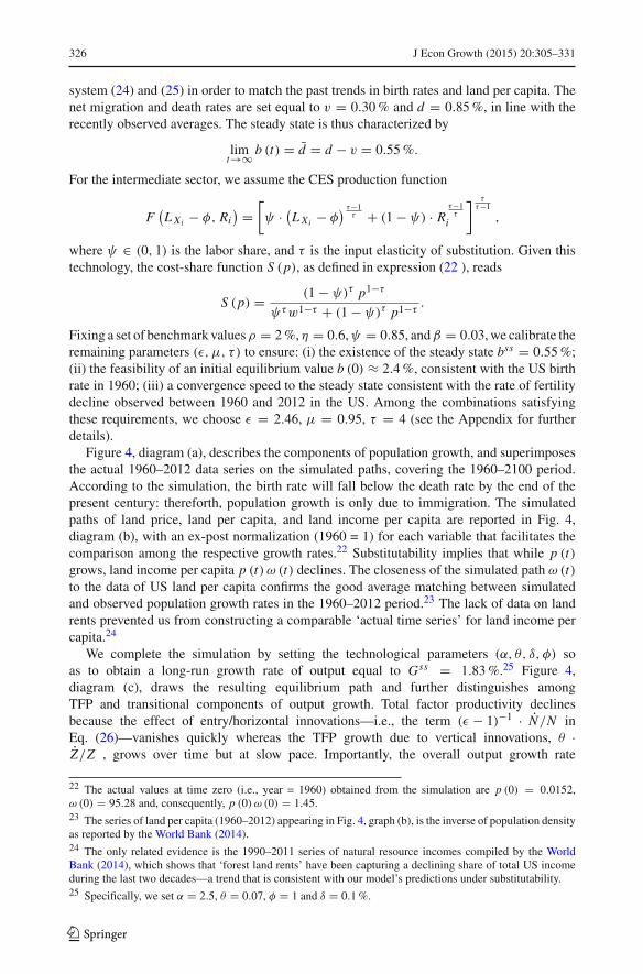
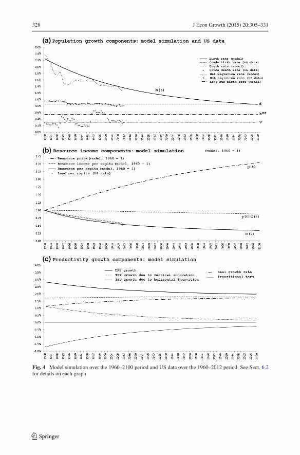
Figure 4, diagram (a), describes the components of population growth, and superimposesthe actual 1960–2012 data series on the simulated paths, covering the 1960–2100 period.According to the simulation, the birth rate will fall below the death rate by the end of thepresent century: thereforth, population growth is only due to immigration. The simulatedpaths of land price, land per capita, and land income per capita are reported in Fig. 4,diagram (b), with an ex-post normalization (1960 = 1) for each variable that facilitates thecomparison among the respective growth rates.22 Substitutability implies that while p (t)grows, land income per capita p (t) ω (t) declines. The closeness of the simulated path ω (t)to the data of US land per capita confirms the good average matching between simulatedand observed population growth rates in the 1960–2012 period.23 The lack of data on landrents prevented us from constructing a comparable ‘actual time series’ for land income percapita.24

We complete the simulation by setting the technological parameters (α, θ, δ, φ) soas to obtain a long-run growth rate of output equal to Gss = 1.83%.25 Figure 4,diagram (c), draws the resulting equilibrium path and further distinguishes amongTFP and transitional components of output growth. Total factor productivity declinesbecause the effect of entry/horizontal innovations—i.e., the term (ε − 1)−1 · N/N inEq. (26)—vanishes quickly whereas the TFP growth due to vertical innovations, θ ·Z/Z , grows over time but at slow pace. Importantly, the overall output growth rate

22 The actual values at time zero (i.e., year = 1960) obtained from the simulation are p (0) = 0.0152,ω (0) = 95.28 and, consequently, p (0) ω (0) = 1.45.23 The series of land per capita (1960–2012) appearing in Fig. 4, graph (b), is the inverse of population densityas reported by the World Bank (2014).24 The only related evidence is the 1990–2011 series of natural resource incomes compiled by the WorldBank (2014), which shows that ‘forest land rents’ have been capturing a declining share of total US incomeduring the last two decades—a trend that is consistent with our model’s predictions under substitutability.25 Specifically, we set α = 2.5, θ = 0.07, φ = 1 and δ = 0.1%.

123

J Econ Growth (2015) 20:305–331 327

G (t) increases over time despite the TFP slowdown, according to the mechanismnoted in Sect. 6.1. The present context allows us to interpret this phenomenon as fol-lows.

When labor and land are substitutes, the transitional resource-income effect in Eq. (26)operates like a resource-income drag in the short run. Infact, when population grows rel-atively fast, the resource price grows quickly, and a relatively high value of p/p > 0keeps the output growth rate low in the short run. As time passes, population growth slowsdown and the same mechanism makes the transitional resource-income effect smaller inabsolute value, pushing up the overall output growth rate during the whole transition—cf.Fig. 4, diagram (c). The fact that the resource-income drag may be quantitatively relevantfor transitional output growth is an interesting result that should deserve careful empiricalscrutiny.

6.3 Demographic shock

This section exploits the benchmark simulation of theUS economy to study the consequencesof a future reduction in the US migration rate. In qualitative terms, the model yields clearpredictions: considering the phase diagram of system (24) and (25), a permanent reductionof the average migration rate, v, induces an upward shift of the ω = 0 locus like the onedepicted in Fig. 5, graph (a). Differently from the income shock studied in Sect. 6.1, themigration shock modifies both the fertility rate bss and the level of per capita resourceωss in the long run. More precisely, the drop in net migration generates a sequence of (i)lower population growth rates and (ii) higher birth rates relative to the pre-shock situation,regardless of whether the economy is initially in the steady state.26 The intuition for result(i) is that a drop in the migration rate is equivalent to an increase in the death rate: thereduction of v directly reduces population growth and thus raises land per capita in the longrun—e.g., from ω′ to ω′′ > ω′ in Fig. 5, graph (a). The intuition for result (ii) is that lowermigration induces labor scarcity and thereby a higher net private benefit from fertility. Itfollows that the sudden drop in net immigration does not translate into an equivalent drop inthe population growth rate because it is partially offset by an increase in the domestic birthrate.

In order to analyze future reductions in the US migration rate, we assume that, at thetime of the shock, the economy is placed to the right of the initial steady state, i.e., land percapita is above the pre-shock steady state ω′ in Fig. 5, graph (a). The qualitative featuresof the transitional dynamics depend on how far land per capita is from ω′ when the shockhits. If it is realtively close (e.g., ω = ωa), the transition features reversion: the previouslydeclining birth rate jumps upwards, and keeps on increasing thereafter. If it is relatively far(e.g., ω = ωb), instead, the birth rate overshoots upward and converges to the new long-runvalue from above.

In our quantitative analysis, we consider the benchmark simulation of the US economyand assume that the net migration rate halves—i.e., v declines from 0.30 to 0.15%—fromyear 2025 onwards. At the time of the shock, land per capita is far from our reference steady

26 To prove this statement, consider Fig. 5, graph (a), and suppose that the economy is initially placed alongany given point along the saddle path leading to the initial steady state

(d ′, ω′). After the shock, the birth rate

jumps upward on the new saddle path leading to the new steady state(d ′′, ω′′) given the pre-shock level of

resource per capita ω′. In such a point, the gap between the after-shock fertility rate and d ′′ is smaller thanthe gap between the pre-shock fertility rate and d ′, which implies that the after-shock population growth rateis lower than the before-shock population growth rate.

123

328 J Econ Growth (2015) 20:305–331

Fig. 4 Model simulation over the 1960–2100 period and US data over the 1960–2012 period. See Sect. 6.2for details on each graph

123

J Econ Growth (2015) 20:305–331 329

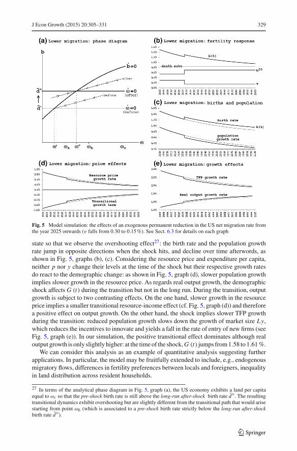
Fig. 5 Model simulation: the effects of an exogenous permanent reduction in the US net migration rate fromthe year 2025 onwards (v falls from 0.30 to 0.15%). See Sect. 6.3 for details on each graph

state so that we observe the overshooting effect27: the birth rate and the population growthrate jump in opposite directions when the shock hits, and decline over time afterwords, asshown in Fig. 5, graphs (b), (c). Considering the resource price and expenditure per capita,neither p nor y change their levels at the time of the shock but their respective growth ratesdo react to the demographic change: as shown in Fig. 5, graph (d), slower population growthimplies slower growth in the resource price. As regards real output growth, the demographicshock affects G (t) during the transition but not in the long run. During the transition, outputgrowth is subject to two contrasting effects. On the one hand, slower growth in the resourceprice implies a smaller transitional resource-income effect (cf. Fig. 5, graph (d)) and thereforea positive effect on output growth. On the other hand, the shock implies slower TFP growthduring the transition: reduced population growth slows down the growth of market size Ly,which reduces the incentives to innovate and yields a fall in the rate of entry of new firms (seeFig. 5, graph (e)). In our simulation, the positive transitional effect dominates although realoutput growth is only slightly higher: at the timeof the shock,G (t) jumps from1.58 to 1.61%.

We can consider this analysis as an example of quantitative analysis suggesting furtherapplications. In particular, the model may be fruitfully extended to include, e.g., endogenousmigratory flows, differences in fertility preferences between locals and foreigners, inequalityin land distribution across resident households.

27 In terms of the analytical phase diagram in Fig. 5, graph (a), the US economy exhibits a land per capitaequal to ωc so that the pre-shock birth rate is still above the long-run after-shock birth rate d ′′. The resultingtransitional dynamics exhibit overshooting but are slightly different from the transitional path that would arisestarting from point ωb (which is associated to a pre-shock birth rate strictly below the long-run after-shockbirth rate d ′′).

123

330 J Econ Growth (2015) 20:305–331

7 Conclusion

This paper investigated the dynamic interdependence of resource scarcity, income and popu-lation in a Schumpeterian model with endogenous fertility. The analysis offers the followingresults. When labor and resources are strict complements or strict substitutes in production,the increase in resource scarcity induced by population growth generates price effects thatmodify income per capita yielding opposite feedback effects on fertility. These price effectscreate a steady state in which population is constant, income per capita grows at a constantendogenous rate, and population size is independent of technology. Under substitutability,this steady state is the system’s global attractor. Under complementarity, instead, it is a sep-arating threshold and the population level follows diverging paths: higher (lower) resourcescarcity generated by the growth (decline) of population increases (decreases) income percapita and fertility rates, implying self-reinforcing feedback effects that drive the economytowards demographic explosion (extinction).

The paper thus proposes a theory of the population level which is consistent with the factthat Planet Earth has a finite carrying capacity of people. This basic characteristic of closedsystems is not captured bybalancedgrowthmodels that feature exponential population growthin the long run. Nonetheless, our theory can be exploited to perform a quantitative analysisof real-world economies. Given the lack of global data, we focused on the US economy as alaboratory to analyze the joint dynamics of population, income, land scarcity and total factorproductivity. Future quantitative research may exploit the benchmark model to include, e.g.,endogenous migratory flows, preference heterogeneity and inequality in land distributionacross households.

References

Ashraf, Q., Lester, A., &Weil, D. N. (2008). When does improving health raise GDP?. NBERWorking Paper14449.

Basener, B., & Ross, D. (2005). Booming and crashing populations and Easter island. SIAM Journal of AppliedMathematics, 65(2), 684–701.

Birdsall, N., & Sinding, S. W. (2001). How and why population matters: New findings, new issues. In N.Birdsall, A. C. Kelley, & S. W. Sinding (Eds.), Population matters: Demographic change, economicgrowth, and poverty in the developing world (pp. 3–23). Oxford: Oxford University Press.

Bloom, D., & Canning, D. (2001). Cumulative causality, economic growth, and the demographic transition. InN. Birdsall, A. C. Kelley, & S. W. Sinding (Eds.), Population matters: Demographic change, economicgrowth, and poverty in the developing world (pp. 165–198). Oxford: Oxford University Press.

Brander, J., & Taylor, M. (1998). The simple economics of Easter island: A Ricardo Malthus model ofrenewable resource use. American Economic Review, 88(1), 119–138.

Bretschger, L. (2013). Population growth and natural resource Scarcity: Long-run development under seem-ingly unfavourable conditions. Scandinavian Journal of Economics, 115(3), 722–755.

Brückner,M., & Schwandt, H. (2014). Income and population growth.Economic Journal Forthcoming. doi:10.1111/ecoj.12152.

Connolly, M., & Peretto, P. F. (2003). Industry and the family: Two engines of growth. Journal of EconomicGrowth, 8, 115–145.

D’Alessandro, S. (2007). Non-linear dynamics of population and natural resources: The emergence of differentpatterns of development. Ecological Economics, 62(3–4), 473–481.

Dinopoulos, E., & Thompson, P. (1998). Schumpeterian growth without scale effects. Journal of EconomicGrowth, 3(4), 313–335.

Doepke, M. (2004). Accounting for fertility decline during the transition to growth. Journal of EconomicGrowth, 9(3), 347–383.

Galor, O. (2005). From stagnation to growth: Unified growth theory. In P. Aghion & S. N. Durlauf (Eds.),Handbook of economic growth (pp. 171–293). Amsterdam: Elsevier.

Galor, O. (2011). Unified growth theory. Princeton, NJ: Princeton University Press.

123

J Econ Growth (2015) 20:305–331 331

Galor, O., & Weil, D. N. (2000). Population, technology and growth: From the Malthusian regime to thedemographic transition. American Economic Review, 110, 806–828.

Good,D.H.,&Reuveny,R. (2009).On the collapse of historical civilizations.American Journal of AgriculturalEconomics, 91(4), 863–879.

Ha, J., & Howitt, P. (2007). Accounting for trends in productivity and R&D: A schumpeterian critique ofsemi-endogenous growth theory. Journal of Money, Credit, and Banking, 33, 733–774.

Hansen, G. D., & Prescott, E. C. (2002). Malthus to Solow. American Economic Review, 92(4), 1205–1217.Jones, L. E., & Tertilt, M. (2008). An economic history of fertility in the US: 1826–1960. In P. Rupert (Ed.),

Frontiers of family economics (Vol. 1). Bingley: Emerald Press.Kelley, A. (2001). The population debate in historical perspective: Revisionism revised. In N. Birdsall, A. C.

Kelley, & S.W. Sinding (Eds.), Population matters: Demographic change, economic growth, and povertyin the developing world (pp. 24–54). Oxford: Oxford University Press.

Kremer, M. (1993). Population growth and technological change: One million BC to 1990. Quarterly Journalof Economics, 108, 681–716.

Laincz, C., & Peretto, P. F. (2006). Scale effects in endogenous growth theory: An error of aggregation, notspecification. Journal of Economic Growth, 11, 263–288.

Lucas, R. (2002). Lectures on Economic Growth. Cambridge, MA: Harvard University Press.Madsen, J. B. (2008). Semi-endogenous versus schumpeterian growth models: Testing the knowledge pro-

duction function using international data. Journal of Economic Growth, 13, 1–26.Madsen, J. B., &Ang, J. B. (2011). Can second-generation endogenous growthmodels explain the productivity

trends in the Asian miracle economies? Review of Economics and Statistics, Forthcoming, 93(4), 1360–1373.

Madsen, J. B., Ang, J. B., & Banerjee, R. (2010). Four centuries of British economic growth: The roles oftechnology and population. Journal of Economic Growth, 15, 263–290.

Malthus, T. R. (1798). An essay on the principle of population. London: St. Paul’s Church-Yard.Peretto, P. F. (1998). Technological change and population growth. Journal of Economic Growth, 3(4), 283–

311.Peretto, P. F. (2012). Resource abundance, growth and welfare: A Schumpeterian perspective. Journal of

Development Economics, 97, 142–155.Peretto, P. F., & Connolly, M. (2007). The manhattan metaphor. Journal of Economic Growth, 12(4), 329–350.Peretto, P. F., & Smulders, S. (2002). Technological distance growth and scale effects. Economic Journal,

112(481), 603–624.Peretto, P. F., & Valente, S. (2013). Growth on a finite planet: Resources, technology and population in the

long run. Working Paper 147, Department of Economics, Duke University.Pezzey, J. C. V. (1992). Sustainable development concepts: An economic analysis.Washington, DC: TheWorld

Bank.Schäfer, A. (2014). Technological change, population dynamics, and natural resource depletion.Mathematical

Social Sciences, 71, 122–136.Smulders, S. (2005). Endogenous technological change, natural resources, and growth. In R. D. Simpson, M.

A. Toman, & R. U. Ayres (Eds.), Scarcity and growth revisited; natural resources and the environmentin the New Millennium (Chap. 8). Baltimore: RFF Press.

Strulik, H., & Weisdorf, J. (2008). Population, food, and knowledge: A simple unified growth theory. Journalof Economic Growth, 13, 169–194.

Taylor, M. S. (2009). Innis Lecture: Environmental crises: past, present, and future. Canadian Journal ofEconomics, 42(4), 1240–1275.

Wang, P., Yip, C. K., & Scotese, C. A. (1994). Fertility choice and economic growth: Theory and evidence.The Review of Economics and Statistics, 76(2), 255–266.

Weil,D.N.,&Wilde, J. (2009).How relevant isMalthus for economic development today?American EconomicReview—Papers and Proceedings, 99(2), 255–260.

World Bank (2014). World Development Indicators 2013. www.worldbank.org. Accessed 1 June 2014.Xepapadeas, A. (2005). Economic growth and the environment. In K.-G. M äler & J. R. Vincent (Eds.),

Handbook of environmental economics. Amsterdam: Elsevier.

123