group 6 nde project

ME 7820 Group Project

Group No- 6

Submitted by-

Praveen Kumar Kumaresan (FX1628)

Harshada Patil (FX4157)

Sathish Kumar Manjulaushankar (FX6865)

Sushma Mallula (FT5826)

Viswa Sai Manoj Mungara (FZ4883)

Chayan Mishra (FX 5634)

Guided By-

Dr. Emmanuel O. Ayorinde

THREE MASS, FOUR SPRING VIBRATORY SYSTEM, WITH AN ATTACHED

VIBRATION ABSORBER WITH A SMALL SPRING AND MASS SYSTEM

M1 = m = 1; K1 = k= 1 (appropriate units)

F_2016 7820 PROJECT GUIDANCE

1.Analyze the horizontal, longitudinal vibration motion of your system (without the appended “absorber”, the

auxiliary system Ma-Ka), assuming frictionless translation, and computing all resonance frequencies.

2.Calculate, Sketch and Anotate (label with values) all the mode shapes.

3. Start the design to obtain values of Ma and Ka that would yield an x2 value (i.e. the motion amplitude of mass

M2) equal to or nearly equal to zero, by trying three sizes (low, medium, large) of values for the auxiliary system,

and reiterating your analyses until you satisfy the project goal (mass and stiffness values that would give us as

near-zero as possible relative amplitude value for M2) for the whole system. In each case of iteration, record the

magnitude of the relative amplitude of mass M2, to be shown as part of your report.

4.Do you think a proper sizing of the auxiliary system can change the amplitude of vibration of the mass to which

the “absorber” system is attached, i.e. M2 here? Give logical, technical reasons.

5.What sizes of Ka and Ma should we use to reduce the amplitude of M2 to practically zero?

6.Comment on the whole exercise and what you think may be learnt from it.

Parameters for Group 6- M2 =1.5m; M3 = 2m; K2 = k; K3 = 2k ; K4 = 3k (Given)

Make a column for these entities.

PART-1

The free body diagrams shown below of each of the masses in the mass-spring system shown above.

(Mass-I)

(Mass-II)

(Mass-III)

(Ma-Ka)

Now the system with considering the auxiliary mass using free body diagram analysis, we could set

up the following equation to solve for the spring coefficient matrix below.

a)𝑚1�̈�1= −𝑘1𝑥1+ 𝑘2 𝑥2− 𝑥1 b) 𝑚2�̈�2= −𝑘2 𝑥2− 𝑥1 + 𝑘3 𝑥3− 𝑥2 + 𝑘𝑎 𝑥𝑎− 𝑥2

c)𝑚3�̈�3= −𝑘4𝑥3− 𝑘3 𝑥3− 𝑥2 d) 𝑚𝑎�̈�𝑎= − 𝑘𝑎 𝑥𝑎− 𝑥2

Shifting the variables around, we get the following,

𝑚1𝑥 1+ 𝑘1+ 𝑘2 𝑥1− 𝑘2𝑥2 = 0 𝑚2𝑥 2− 𝑘2 𝑥1+ 𝑘2+ 𝑘3+ 𝑘𝑎 𝑥2− 𝑘3𝑥3 − 𝑘𝑎𝑥𝑎 = 0

𝑚3𝑥 3− 𝑘3𝑥2+ 𝑘3+ 𝑘4 𝑥3 = 0 𝑚𝑎𝑥 𝑎− 𝑘𝑎𝑥2+ 𝑘𝑎𝑥𝑎= 0

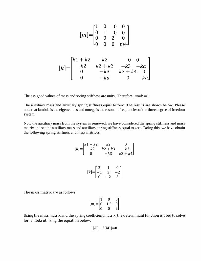
Now the above equations into matrix form, we obtain the mass and spring coefficient matrices below.

[𝑚]=[

1 0 0 00 1 0 000

00

2 00 𝑚4

]

[𝑘]=[

𝑘1 + 𝑘2 𝑘2 0 0−𝑘2 𝑘2 + 𝑘3 −𝑘3 −𝑘𝑎00

−𝑘3−𝑘𝑎

𝑘3 + 𝑘4 00 𝑘𝑎

]

The assigned values of mass and spring stiffness are unity. Therefore, 𝑚=𝑘 =1. The auxiliary mass and auxiliary spring stiffness equal to zero. The results are shown below. Please

note that lambda is the eigenvalues and omega is the resonant frequencies of the three degree of freedom

system.

Now the auxiliary mass from the system is removed, we have considered the spring stiffness and mass

matrix and set the auxiliary mass and auxiliary spring stiffness equal to zero. Doing this, we have obtain

the following spring stiffness and mass matrices.

[𝒌]=[𝑘1 + 𝑘2 𝑘2 0−𝑘2 𝑘2 + 𝑘3 −𝑘30 −𝑘3 𝑘3 + 𝑘4

]

[𝑘]=[2 1 0−1 3 −20 −2 5

]

The mass matrix are as follows

[𝑚]=[1 0 00 1.5 00 0 2

]

Using the mass matrix and the spring coefficient matrix, the determinant function is used to solve

for lambda utilizing the equation below.

|[𝑲]− 𝜆[𝑴]|=𝟎

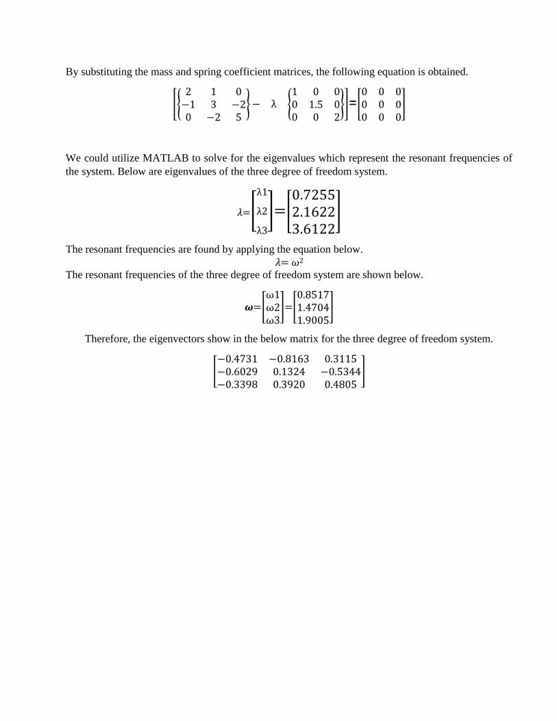
By substituting the mass and spring coefficient matrices, the following equation is obtained.

[{2 1 0−1 3 −20 −2 5

}− λ {1 0 00 1.5 00 0 2

}]=[0 0 00 0 00 0 0

]

We could utilize MATLAB to solve for the eigenvalues which represent the resonant frequencies of

the system. Below are eigenvalues of the three degree of freedom system.

𝜆=[λ1

λ2

λ3

]=[0.72552.16223.6122

]

The resonant frequencies are found by applying the equation below.

𝜆= 𝜔2

The resonant frequencies of the three degree of freedom system are shown below.

𝝎=[ω1ω2ω3

]=[0.85171.47041.9005

]

Therefore, the eigenvectors show in the below matrix for the three degree of freedom system.

[−0.4731 −0.8163 0.3115−0.6029 0.1324 −0.5344−0.3398 0.3920 0.4805

]

PART-2

The mode shapes of the three degree of freedom mass-spring system shown below.

I. First Mode Shape-

II. Second Mode Shape-

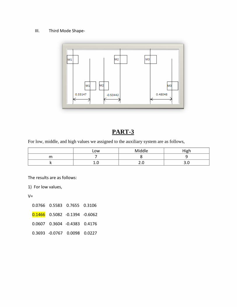
III. Third Mode Shape-

PART-3

For low, middle, and high values we assigned to the auxiliary system are as follows,

Low Middle High

m 7 8 9

k 1.0 2.0 3.0

The results are as follows:

1) For low values,

V=

0.0766 0.5583 0.7655 0.3106

0.1466 0.5082 -0.1394 -0.6062

0.0607 0.3604 -0.4383 0.4176

0.3693 -0.0767 0.0098 0.0227

2) For Middle values,

V=

0.1029 0.6516 0.6983 0.2777

0.1950 0.4068 -0.1438 -0.6652

0.0814 0.3618 -0.4892 0.3509

0.3390 -0.0903 0.0184 0.0401

3) For Maximum values,

V=

0.1125 0.7386 0.6192 0.2416

0.2127 0.3193 -0.1440 -0.7062

0.0890 0.3425 -0.5384 0.2914

0.3169 -0.0862 0.0253 0.0513

PART-4

Many a times, a vibratory system under forced vibration is required to run near resonance i.e. the

excitation frequency is close to the natural frequency of the system. Under such a situation, the response

of the system can be large and we must try to reduce it by taking some measure. By attaching a separate

smaller spring-mass system, an auxiliary system, to the main system the vibration of the main system

can be reduced, drastically, if the mass and the stiffness of the auxiliary system are properly calculated,

i.e. if the auxiliary system is tuned to the natural frequency of the main system and the excitation

frequency.

Adding stiffness and mass to the system, results in change of resonant frequencies and mode shapes of

the system. The reason that we add stiffness to the auxiliary system is to dampen the amplitude of the

second mass. Normally, we are concerned with the first mode, so the objective here is to find an

optimized combination of mass and stiffness of the auxiliary system to reduce the amplitude of mass 2

in the first mode.

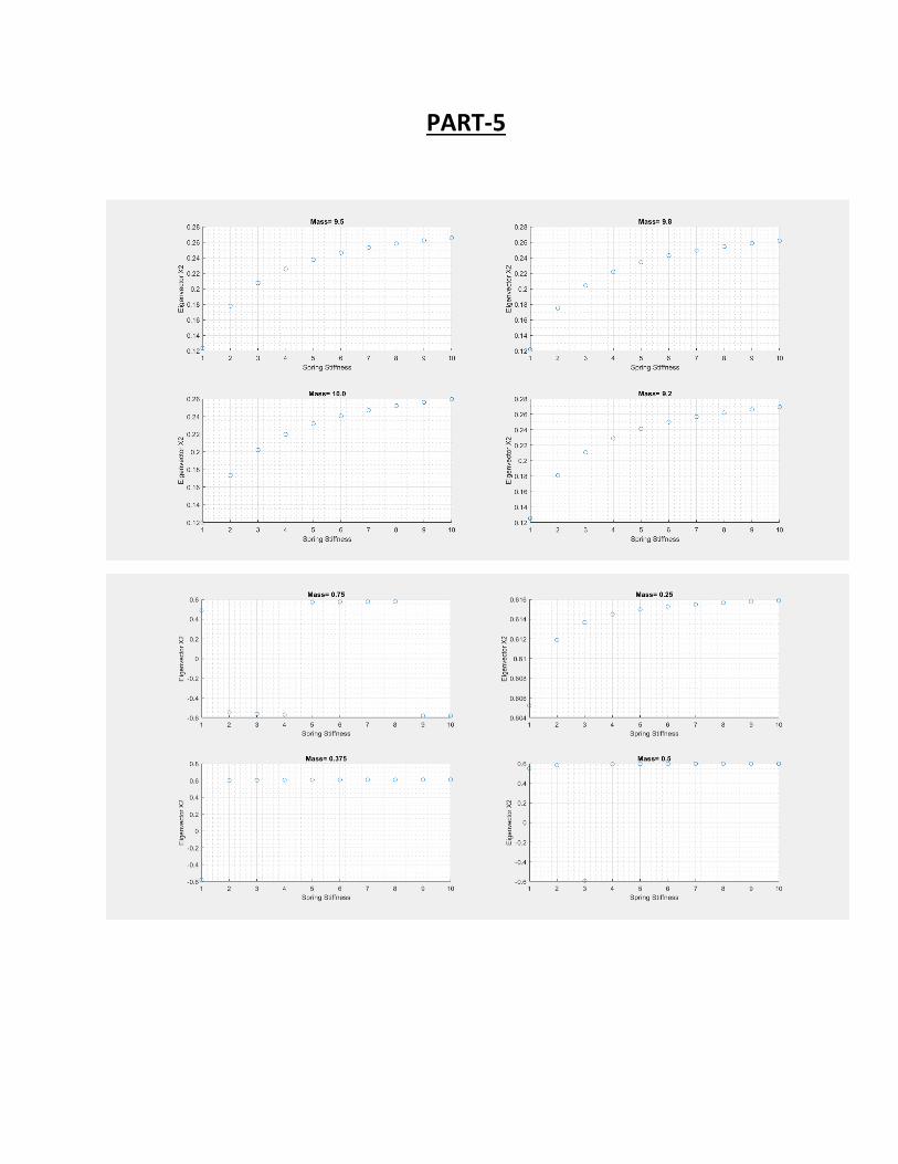
PART-5

OBSERVATION:

Value is never zero because there is no damper as we increase mass the value approaches zero but will

get to zero.

In all the three graphs it can be clearly observed that as the stiffness constant increases the amplitude

also increases but here we are more inclined towards finding the right combination which decreases the

amplitude to zero. Even though the amplitude cannot be zero totally we would rather choose the

combination where it approaches to closer to zero.

If we see the trend in the graph, the amplitude of M2 will never be zero but it can get as close to zero

which is 0.02 in this case. So the best combination for lowest amplitude possible is Ma=9.5 & Ka=0.1

and for which the amplitude is 0.25.

PART-6

Amplitude is equation given by

Hypothetically, the reaction of an un-damped framework relies on upon the initial displacement, speed

and natural frequency of the framework. As the initial two terms are not considered in this work, the

main thing influencing the reaction is the regular frequencies of the framework. Expanding mass of

assistant framework does not really bring about decreasing the amplitude of mass 2. Moreover,

expanding the solidness does not roll out any improvement to framework from a specific esteem. The

best mix to diminish the adequacy of mass 2 happens when the mass is 9.5 and stiffness 0.25. It is sure

that expanding mass and firmness all the while doesn’t influence the normal frequency. Evidently in

this issue, impacts of mass are far more than the impact of firmness. That is to state, this framework is

likely to change of mass of helper framework as opposed to the solidness. Since it was watched that

after a specific esteem for stiffness of helper framework, there is no adjustment in the sufficiency of

the second mass.

Appendix (MATLAB Code)

clear all

m1=1; m2=1; m3=2; k1=1; k2=1; k3=2; k4=3;

for ka=1:10

ma1=0.75;

K= [k1+k2 -k2 0 0; -k2 k2+k3+ka -k3 -ka; 0 -k3 k3+k4 0; 0

-ka 0 ka];

M= [m1 0 0 0; 0 m2 0 0; 0 0 m3 0; 0 0 0 ma1];

[V1,D1]=eig(K,M);

X(ka)=V1(2,1);

disp(V1);

disp(D1);

end

subplot(2,2,1);

scatter(1:10,X);

grid on;

grid minor;

xlabel('Spring Stiffness');

ylabel('Eigenvector X2');

title('Mass= 0.75');

for ka=1:10

ma1=0.25;


-ka 0 ka];

M= [m1 0 0 0; 0 m2 0 0; 0 0 m3 0; 0 0 0 ma1];

[V2,D2]=eig(K,M);

X(ka)=V2(2,1);

disp(V2);

disp(D2);

end

subplot(2,2,2);

scatter(1:10,X);

grid on;

grid minor;




for ka=1:10

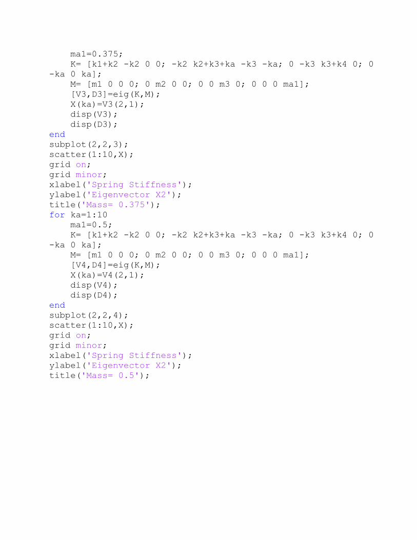
ma1=0.375;


-ka 0 ka];

M= [m1 0 0 0; 0 m2 0 0; 0 0 m3 0; 0 0 0 ma1];

[V3,D3]=eig(K,M);

X(ka)=V3(2,1);

disp(V3);

disp(D3);

end

subplot(2,2,3);

scatter(1:10,X);

grid on;

grid minor;




for ka=1:10

ma1=0.5;


-ka 0 ka];

M= [m1 0 0 0; 0 m2 0 0; 0 0 m3 0; 0 0 0 ma1];

[V4,D4]=eig(K,M);

X(ka)=V4(2,1);

disp(V4);

disp(D4);

end

subplot(2,2,4);

scatter(1:10,X);

grid on;

grid minor;



title('Mass= 0.5');

group 6 nde project

Documents