ground displacement in a fault zone in the presence of

Abstract. Friction on faults controls slip distribution in response to tectonic stress:the friction distribution can be simplified by considering locked zones (asperities)surrounded by aseismic slipping zones. The aseismic slip of fault sections has animportant role in concentrating stress on the asperities and in producing their failure.The slow ground displacement in fault zones is measurable through classic or spatialgeodetic techniques and may help to localize the greater asperities on faults.Therefore accurate geodetic measurements in fault zones may be used to evaluatethe seismic hazard in the region. We represent the Earth’s crust by an elastic,homogeneous and isotropic half-space, including a plane normal fault. A lockedasperity is considered on the fault, while the surrounding area of the fault surfaceundergoes a uniform slip. The surface displacement field is analyzed in the presenceand in the absence of the asperity; the influence of the asperity shape, size and depthis studied also varying the dip angle of the fault. We conclude that an asperity, whosearea is about 1 km2, determines a surface displacement of mm order, when its centreis placed at depths ranging from 5 to 10 km and the surrounding fault area slips bytens of centimeters: in this case an asperity with an area of about 5×5 km2 could bereasonably localized by current geodetic measurements.

1. Introduction

Earthquakes result when the Earth’s crust fails in response to accumulated deformation.Geodetic measurements document the crustal deformation leading to these failures and thedeformation resulting from them. For both earthquakes and aseismic fault motions, geodetic

VOL. 40, N. 2, pp. 95-110; JUNE 2000BOLLETTINO DI GEOFISICA TEORICA ED APPLICATA

Corresponding author: M. Dragoni; Dipartimento di Fisica, Settore di Geofisica, Università di Bologna, VialeB. Pichat 8, Bologna, Italia; phone: +39 02 23996504; fax +39 02 23996530; e-mail:[email protected]

© 2000 OGS

Ground displacement in a fault zonein the presence of asperities

S. SANTINI(1), A. PIOMBO

(2) and M. DRAGONI(2)

(1) Istituto di Fisica, Università di Urbino, Italy(2) Dipartimento di Fisica, Settore di Geofisica, Università di Bologna, Italy

(Received June 24, 1999; accepted May 17, 2000)

95

96

Boll. Geof. Teor. Appl., 41, 95-110 SANTINI et al.

measurements constrain physical models of the processes that cause such events. The use of leveling, GPS and SAR interferometry (InSAR) data allows us to determine the

displacement field at the Earth’s surface associated with fault slip. In particular, whereasmeasurements by conventional and space-based geodetic methods, such as GPS, can moreaccurately determine the displacement vectors for a network of points, InSAR can provide muchdenser spatial coverage of the ground displacement.

The observed variability in the seismic phenomenology is attributed to the mechanicheterogeneity of the fault surfaces. The asperity model of faults assumes that earthquakes are aconsequence of the fast failure of one or more asperities, occurring when the tectonic stress,increasing over a long period of time, overcomes the resistance of the asperity. The search forasperities on active faults is therefore a fundamental step towards a deeper understanding of theseismic source and its dynamics.

Several methods can be used to recognize and locate asperities: the measurement of grounddeformation; the observation of seismicity patterns; the analysis of seismic records of pastearthquakes (both strong motions and teleseismic waves); and, in particular cases, geologicobservations.

If the study of seismicity provides basic information about the failure of strong fault patches,only the observation of slow ground deformation can give direct information about areas whichslip aseismically. In fact, it is conceivable that in the time interval between two large earthquakeson the same fault segment (interseismic phase), the relative plate motion along a plate boundaryis partly accommodated by the aseismic slip of faults. The contrast between the locked areas(asperities) and the freely slipping areas on a fault surface is detectable at the Earth’s surface bygeodetic techniques. Therefore, ground deformation measurements can play a crucial role in thesearch for asperities, in particular if part of the interseismic slip is aseismic.

Attempts to recognize asperities on the San Andreas Fault, in particular on the Parkfieldsegment, were made by several authors (Slawson and Savage, 1983; Bakun and Lindh, 1985;Stuart et al., 1985; Tse et al., 1985; Harris and Segall, 1987; Stuart and Tullis, 1995).

In order to evaluate the pattern and magnitude of ground deformation due to asperities,Dragoni (1988) considered a model in which asperities of different shapes, sizes and depths arepresent on a vertical strike-slip fault embedded in an elastic half-space. In this paper in order toimprove the interpretation of geodetic measurements in terms of asperities for a wider number ofsituations, we calculate the displacement and tilt fields produced by the presence of asperities onnormal faults with different dip angles, embedded in an elastic half-space. Such a model couldbe usefully employed for the seismogenic structures of the Apenninic chain, where an increasingamount of geodetic data is becoming available.

2. The model

Let us consider an elastic, homogeneous and isotropic half-space, occupying the region x3 ≤ 0in a Cartesian coordinate system (Fig. 1a), and assume that a half-plane represents a normal faultsurface intersecting the Earth’s surface with a dip angle δ. As is usual for the Earth’s crust, it is

assumed that the Lamé constants are equal (Poisson solid) and λ = μ = 3 × 1010 Pa. In the case of

a rectangular dislocation, the displacement field at the Earth’s surface can be obtained by

available analytical solutions (e.g. Okada, 1985). The x1 axis is parallel to the fault strike and

contains the projection of the bottom side of the dislocation on the Earth’s surface.

It is assumed that friction on the fault is not homogeneous, but that asperities are present.

According to the asperity model, during the interseismic phase, the fault slips aseismically or

with small earthquakes, corresponding to smaller asperity failures. We assume that a single

dominant asperity is present on the fault: this asperity remains locked, while the remaining part

of the fault slips aseismically in a uniform fashion by an amount U. The displacement field

produced by dislocations, including asperities, can be obtained by suitably combining solutions

for dislocations.

97

Boll. Geof. Teor. Appl., 41, 95-110Ground displacement in the presence of asperities

Fig. 1 - (a) The model: the green area indicates a slipping zone on a normal fault and the red one a locked zone(asperity). (b) Case of a finite-area dislocation including an asperity: z is the depth of the bottom size of the dislocation,d is the same quantity for the asperity and D is the distance of fault trace from the x1 axis.

98


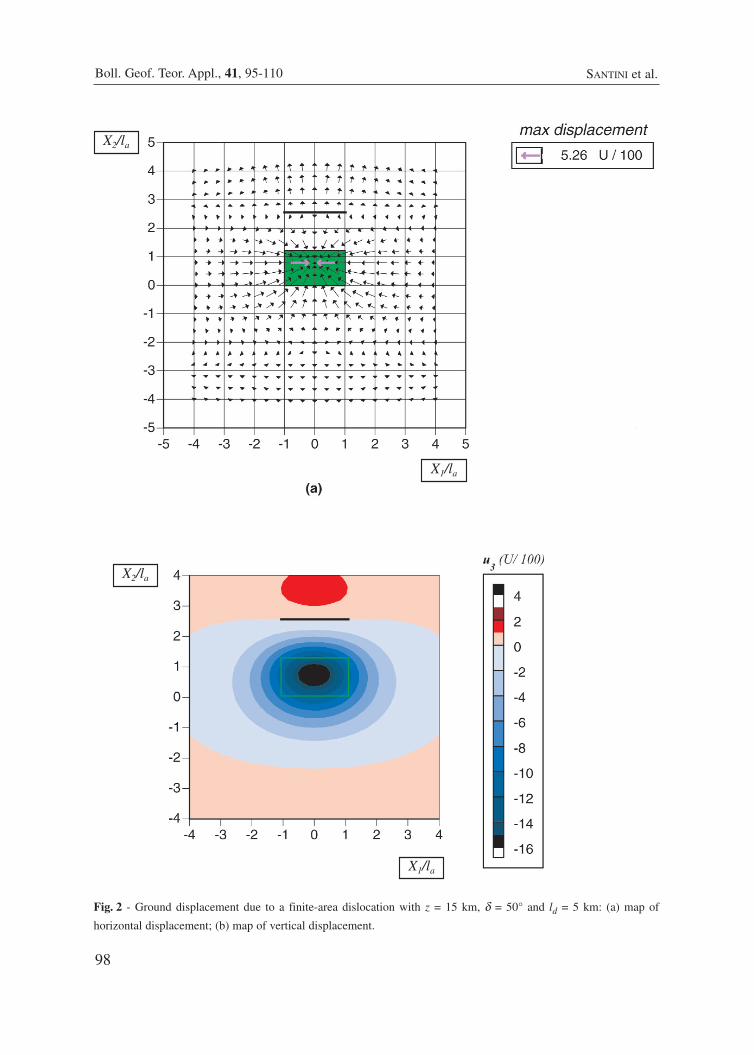
Fig. 2 - Ground displacement due to a finite-area dislocation with z = 15 km, δ = 50° and ld = 5 km: (a) map of

horizontal displacement; (b) map of vertical displacement.

X1/la

X1/la

X2/la

X2/la

99


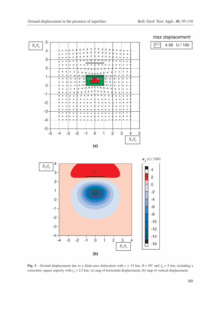
Fig. 3 - Ground displacement due to a finite-area dislocation with z = 15 km, δ = 50° and ld = 5 km, including aconcentric square asperity with la = 2.5 km: (a) map of horizontal displacement; (b) map of vertical displacement.

X2/la

X2/la

X1/la

X1/la

We consider asperities and dislocations with rectangular shapes and find the solutions in thepresence of asperities by considering the asperity as a fault region where the slip is opposite tothat of the dislocation (Fig. 1b). We call z the depth of the bottom side of dislocations and d thesame quantity for asperities. For simplicity, we examine the case of a square dislocation and asquare asperity having the same centre.

We indicate with ud (x1, x2; U, ld) the ground displacement in the case of a square dislocationwith a side of half-length ld and a slip amplitude U; accordingly, the effect of a square asperitywith a side of half-length la can be indicated as ud (x1, x2; -U, la). Since U is a multiplying factorin the displacement, one can write

The total displacement field at the Earth’s surface is obtained by adding the contributions ofthe dislocation and the asperity:

In the case of a square asperity on a half-plane fault, the displacement components u2 and u3

are obtained by adding a uniform slip of the fault walls to the corresponding components ofground displacement due to the asperity:

where D is the distance from the x1 axis to the fault trace

The component x1 is given by

Another useful quantity to be measured at the Earth’s surface is ground tilt, the components ofwhich are defined as

u u1 1d( , ) ( , ; , )x x x x U la1 2 1 2=

D d= cotan δ

u u

u3

3d

3d

( , )sin ( , ; , )

sin ( , ; , ) x x

Ux x U l x D

Ux x U l x D

a

a

1 2

1 2 2

1 2 2

2

2

=− >

− − <

⎧

⎨⎪⎪

⎩⎪⎪

δ

δ

u x x

Ud ud x x U la x D

Ud ud x x U la x D

2 1 22 2 1 2 2

2 2 1 2 2

( , )sin ( , ; , )

sin ( , ; , ) =

− >

− − <

⎧

⎨⎪⎪

⎩⎪⎪

u u u( , ) ( , ; , ) ( , ; , )x x x x U l x x U la a1 2 1 2 1 2= −d d

u ud d( , ; , ) ( , ; , )x x U l x x U la a1 2 1 2− = −

100


(1)

(2)

(3)

(4)

(5)

(6)

101


Fig. 4 - (a) Curves of u3 component along the x2 axis for the case of Fig. 3 (red) and for an appropriate dislocation ofsmaller area without asperity (blue) (for parameters see text).

From the solution for a square asperity, it is easy to obtain the analytical solution for any asperity,with a polygonal contour. As a consequence, it is possible to model the presence of asperitieswith any shape.

3. Discussion

To evaluate the effect on ground displacement of the presence of an asperity on a fault plane,first we consider the displacement field due to a square dislocation; secondly, we examine thecase when an asperity is present inside the dislocation. In Fig. 2, the components of displacementproduced by a square dislocation are shown for δ = 50°, ld = 5 km and z = 15 km; in Fig. 3 thedisplacement field produced by the same dislocation, including a square asperity of side la = 2.5km, is shown. Note that vertical displacement reaches its maximum values along the x2 axis.Negative values of vertical displacement indicate subsidence and positive values indicate uplift,since the x3 axis points upward. The presence of an asperity in the dislocation produces anincrease of the area which is affected by significant uplift, but a decrease of the maximumvertical displacement. For U = 50 cm, the maximum displacement in the case of Fig. 2 is about8 cm and in the case of Fig. 3 is about 7 cm. The maximum absolute values of grounddisplacement are found in correspondence to the centre of the projection on the Earth’s surfaceof the dislocation.

Because the aim of this paper is the interpretation of geodetic measurements, in the followingwe consider the vertical displacement field along the x2 axis where u3 is maximum.

It is interesting to evaluate whether the effects of an asperity inside a dislocation can be modeledby a dislocation with a smaller area but without asperity. Fig. 4a shows that the vertical displacementalong the x2 axis, for the case in Fig. 3, has the same minimum value as that due to a concentricdislocation with ld = 4.55 km but without asperity. The presence of an asperity causes a differentu3pattern and in particular a shift from the fault trace of the position of maximum uplift. Sincegeodetic measurements can have centimetre point positioning accuracies from several millimetres to1 cm, the difference between the two curves of Fig. 4a must be at least of this magnitude for anappropriate interval of x2 in order to distinguish between the two different situations. Fig. 4b showsthat it can be achieved for an amount of slip of 50 cm and that there are two regions along the x2 axis,3 and 5 km wide respectively, where the difference between two cases can be measured.

In the case of a half-plane dislocation, Fig. 5 shows the displacement field for an asperity withd = 15 km, la = 2.5 km, δ = 45°; Fig. 6 shows the same case but for d = 10 km. We note that thepattern of ground displacement varies appreciably, but the maximum values are about constant.As expected, the area of maximum displacement increases for decreasing asperity depths.

We can conclude that the presence of an asperity on a fault plane may change the grounddisplacement field appreciably and, in favourable cases, can allow the location of locked patches.

tu

xii

i

= =∂∂

3 1 2 ,

102


(7)

103


Fig. 5 - Maps of horizontal (a) and vertical displacement (b) in the case of an asperity included in a half-plane

dislocation: z = 15 km, δ = 45° and la = 5 km.

104


Fig. 6 - Maps of horizontal (a) and vertical displacement (b) in the case of an asperity included in a half-plane

dislocation: z = 10 km, δ = 45° and la = 5 km.

To describe the observed surface deformation, it is interesting to evaluate the effects of thevariation of model parameters on the ground displacement pattern. In particular, variations of themodel parameters induce changes in the u3 curves: an increase in asperity depth causes both adecrease in the maximum value of u3 and an increase in the distance between fault trace and theposition of maximum (Fig. 7); an increase in dip angle causes both a decrease in the maximumand a decrease in the distance between fault trace and maximum position (Fig. 8); an increase inasperity area causes both an increase in the maximum and a decrease in the distance betweenfault trace and maximum position (Fig. 9). Obviously, the ground displacement increases as thesize of the asperity increases and its depth decreases.

105


Fig. 7 - Vertical displacement u3 for different values of d, in the case of a half-plane dislocation: la = 5 km and δ = 45°.

For a fault dip of 45°, Fig. 10 shows vertical displacement for an asperity with la = 2.5 km,inside a concentric dislocation with side length increasing up to the Earth’s surface and z = 15km; we note that a larger side of the dislocation causes a larger vertical ground displacement anda shift of position of its maximum and minimum.

Fig. 11 shows the tilt fields along the x2 axis for the cases shown in Fig. 4; the dashed lineindicates the curve of the difference between the two cases. For U = 50 cm tilts of several μradare produced. This indicates that the presence of an asperity on the fault plane can be appreciatedalso by tilt measurements.

106


Fig. 8 - Vertical displacement u3 for different values of angle δ, in the case of a half-plane dislocation: d = 15 km and

la = 5 km.

The location of an asperity on a fault by geodetic measurements may allow us to evaluate theseismogenic potential of the asperity itself. In fact, we can define a potential seismic moment Mp

of the asperity as the maximum value of the seismic moment that can be released in the failureof the asperity, calculated as

where μ is the rigidity of the elastic medium, A is the area of the asperity and U is the slip of the

M AUp = μ

107


Fig. 9 - Vertical displacement u3 for different values of la, in the case of a half-plane dislocation: d = 10 km and

δ = 45°.

(8)

surrounding fault area. The seismic moment Mp is released if during the earthquake the asperityslips by an amount U, so that the total displacement is uniform on the fault after the earthquake.With la= 2.5 km and U = 50 cm, we have Mp = 1.5 × 1018 N m, which corresponds to a magnitude-6 earthquake according to empirical relations (e.g. Kasahara, 1981).

The actual seismic moment may be greater than the value given in Eq. (8) if a larger area than

108


Fig. 10 - Vertical displacement u3 for a finite-area dislocation in presence of an asperity for different values of ld:

z = 15 km, δ = 45° and la = 2.5 km.

the asperity ruptures during the earthquake. In the Parkfield segment of the San Andreas fault,for which accurate data are available, asperities with sizes in the order of several kilometres havebeen detected (Stuart et al.,1985; Harris and Segall, 1987).

4. Conclusions

Using leveling, GPS and InSAR data, it is now possible to study regional deformation fieldsand even to zoom in on individual faults. Geodetic measurements allow us to produce a completepicture of the ground displacement field. Post-seismic deformation studies exemplify howgeodetic data are essential to understanding the aseismic fault behavior and the process of strainaccumulation and release in a seismogenic region. Combining seismic and geodetic data shouldallow identification and characterization of active faults.

The model presented in this paper suggests how the displacement at the Earth’s surface canbe affected by the presence of asperities on active faults. The displacement and tilt fields can bevery complex even in the case of relatively simple asperity shapes as considered in this paper.The inversion and the interpretation of geodetic measurements can give information about thedepth, dip angle and area of the asperities, the amount of the aseismic fault slip and the potentialseismic moment of the asperity. The interpretation of geodetic data with the present model startsfrom knowledge of the position and the orientation of the fault. This indicates that reliableinterpretations can be given only in the presence of sufficiently dense geodetic networks.

109


Fig. 11 - Tilt component t2 along the x2 axis the case of Fig. 4; the dashed line is the difference between the two curves.

We have shown that asperities, the failure of which can produce potentially damagingearthquakes (i.e. shallow asperities producing earthquake magnitudes ≥ 6), can be detected byaccurate geodetic measurements.

Acknowledgments. This research has been carried out in the framework of grant ARS-98-68 of the Agenzia SpazialeItaliana.

References

Bakun W. H. and Lindh A. G.; 1985: The Parkfied, California, prediction experiment. Earthq. Predict. Res., 3, 285-304.

Dragoni M.; 1988: Role of geodetic measurements in the detection of fault asperities. In: P. Baldi and S. Zerbini (eds),Proc. Third Int. Conf. on the WEGENER/MEDLAS Project, Bologna, 129-146.

Harris R. A. and Segall P.; 1987: Detection of a locked zone at depth on the Parkfield, California, segment of the SanAndreas Fault. J. Geophys. Res., 92, 7945-7962.

Kasahara K.; 1981: Earthquake mechanics. Cambridge Earth Science Series, Cambridge University Press, Cambridge,248 pp.

Okada Y.; 1985: Surface deformation due to shear and tensile faults in a half-space. Bull. Seism. Soc. Amer., 75,1135-1154.

Slawson W. F. and Savage J. C.; 1983: Deformation near the junction of the creeping and locked segments of the SanAndreas Fault, Cholame Valley, California (1970-1980). Bull. Seism. Soc. Amer., 73, 1407-1414.

Stuart W. D., Archuleta R. J. and Lindh A. G.; 1985: Forecast model for moderate earthquakes near Parkfield,California. J. Geophys. Res., 90, 592-604.

Stuart W. D. and Tullis T. E.; 1995: Fault model for preseismic deformation at Parkfield, California. J. Geophys. Res.,100, 24 079-24 099.

Tse S. T., Dmowska R. and Rice J. R.; 1985: Stressing of locked patches along a creeping fault. Bull. Seism. Soc.Amer., 75, 709-736.

110


ground displacement in a fault zone in the presence of

Documents