grey water footprint f accounting b...
TRANSCRIPT
GREY WATER FOOTPRINT
ACCOUNTING
TIER 1 SUPPORTING GUIDELINES
N.A. FRANKE
H. BOYACIOGLU
A.Y. HOEKSTRA
DECEMBER 2013
VALUE OF WATER RESEARCH REPORT SERIES NO. 65

GREY WATER FOOTPRINT ACCOUNTING
TIER 1 SUPPORTING GUIDELINES
N.A. FRANKE1,*
H. BOYACIOGLU2
A.Y. HOEKSTRA3
DECEMBER 2013
VALUE OF WATER RESEARCH REPORT SERIES NO. 65
1 Water Footprint Network, Enschede, The Netherlands
2 Department of Environmental Engineering, Dokuz Eylul University, Izmir, Turkey 3 Twente Water Centre, University of Twente, Enschede, The Netherlands
*Corresponding author: Nicolas A. Franke, [email protected]
© 2013 N.A. Franke, H. Boyacioglu, A.Y. Hoekstra
Published by:
UNESCO-IHE Institute for Water Education
P.O. Box 3015
2601 DA Delft
The Netherlands
The Value of Water Research Report Series is published by UNESCO-IHE Institute for Water Education, in
collaboration with University of Twente, Enschede, and Delft University of Technology, Delft.
All rights reserved. No part of this publication may be reproduced, stored in a retrieval system, or transmitted, in
any form or by any means, electronic, mechanical, photocopying, recording or otherwise, without the prior
permission of the authors. Printing the electronic version for personal use is allowed.
Please cite this publication as follows:
Franke, N.A., Boyacioglu, H. and Hoekstra, A.Y. (2013) Grey water footprint accounting: Tier 1 supporting
guidelines, Value of Water Research Report Series No. 65, UNESCO-IHE, Delft, the Netherlands.
Acknowledgement
We would like to thank the Grey Water Footprint Expert Panel, for their input and feedback in the process of
developing these supporting guidelines: Colin Brown (University of York – UK), Richard Coupe (U.S.
Geological Survey, Pearl, Mississippi), Julian Dawson* (The James Hutton Institute, Craigiebuckler, Scotland
UK), Mark Huijbregts (Radboud University Nijmegen, The Netherlands), Himanshu Joshi (Indian Institute of
Technology at Roorkee, India), Bernd Lennartz (Faculty for Agricultural and Environmental Sciences Rostock
University, Germany), Roger Moussa (French National Institute of Agricultural Research, France), Alain
Renard (Sustainable Business Development, C&A, Brussels), Ranvir Singh (Massey University, New Zealand),
Merete Styczen (KU-Life, Copenhagen, Denmark), Aaldrik Tiktak (Netherlands Environmental Assessment
Agency, Netherlands), and Matthias Zessner (Vienna University of Technology, Austria). Special thanks also to
Phillip Chamberlain and the C&A Foundation for funding this project.
* In memory of Julian Dawson who tragically passed away in the period of finalizing the guidelines.
Contents
1. Introduction ..................................................................................................................................................... 7 2. Objective and scope of the guidelines ............................................................................................................. 9 3. How to calculate the grey water footprint ..................................................................................................... 11 4. How to estimate the leaching-runoff fraction for diffuse pollution sources.................................................. 15
4.1. Overview ............................................................................................................................................... 15 4.2. Nitrogen ................................................................................................................................................ 18 4.3. Phosphorus ............................................................................................................................................ 20 4.4. Metals .................................................................................................................................................... 23 4.5. Pesticides ............................................................................................................................................... 25
5. Which maximum allowable concentration to use ......................................................................................... 29 5.1. Introduction ........................................................................................................................................... 29 5.2. Nitrogen and phosphorous .................................................................................................................... 30 5.3. Metals & inorganics, pesticides & organics, and additional water quality parameters ......................... 31
6. What natural background concentration to use ............................................................................................. 37 References ............................................................................................................................................................ 39
Appendices
I. Supporting information ..................................................................................................................................... 43 General information ..................................................................................................................................... 43 Contaminant factors ..................................................................................................................................... 43 Soil information ........................................................................................................................................... 43 Nutrient surplus ............................................................................................................................................ 44 Maximum allowable concentrations ............................................................................................................ 44 Natural background concentrations .............................................................................................................. 44
II. Leaching-runoff influencing factor maps ......................................................................................................... 45 III. Agricultural management practice questionnaire ........................................................................................... 55 IV. Example on how to calculate the grey water footprint based on these guidelines .......................................... 57

1. Introduction
The grey water footprint (GWF) is an indicator of the water volume needed to assimilate a pollutant load that
reaches a water body. As an indicator of water resources appropriation through pollution, it provides a tool to
help assess the sustainable, efficient and equitable use of water resources. The application of the GWF by
different stakeholders (from companies to environmental ngo’s and governmental institutions) has shown its
diverse usability as an indicator for water resource management.
The GWF is defined as part of the global water footprint standard in The Water Footprint Assessment Manual
(Hoekstra et al., 2011). The GWF is an indicator of the amount of freshwater pollution that can be associated
with an activity. The GWF of a product will depend on the GWFs of the different steps of its full production and
supply chain. The GWF is defined as the volume of freshwater that is required to assimilate a load of pollutants
to a freshwater body, based on natural background concentrations and existing ambient water quality standards.
The GWF is calculated as the volume of water that is required to dilute pollutants (chemical substances) to such
an extent that the quality of the water remains above agreed ambient water quality standards.
The Water Footprint Assessment Manual recommends a three-tier approach for estimating diffuse pollution
loads entering a water body. The three-tier approach was the outcome of the Grey Water Footprint Working
Group of the Water Footprint Network (WFN) in 2010 and is analogue to the tier approach proposed by the
Intergovernmental Panel on Climate Change for estimating greenhouse gas emissions (IPCC, 2006). From tier 1
to 3, the accuracy of estimating the load reaching a water body increases, but the feasibility of carrying out the
analysis decreases because of the increasing data demand.
Tier 1 simply uses a leaching-runoff fraction to translate data on the amount of a chemical substance applied to
the soil to an estimate of the amount of the substance entering the groundwater or surface water system. The
fraction is to be derived from existing literature and will depend on the chemical considered. This tier-1 estimate
is sufficient for a first rough estimate, but obviously does not describe the different pathways of a chemical
substance from the soil surface to surface or groundwater and the interaction and transformation of different
chemical substances in the soil or along its flow path.
Tier 2 applies standardized and simplified model approaches and can be used based on relatively easily
obtainable data (such as the chemical properties of the chemical substance considered and the topographic,
climatic, hydrologic and soil characteristics of the environment in which the chemical substance is applied).
These simple and standardized model approaches should be derived from more advanced and validated models.
Tier 3 uses sophisticated modelling techniques and/or intensive measurement approaches. Since this approach is
very laborious, available resources should allow for it and the purpose of application should warrant it. Whereas
detailed physically-based models of contaminant flows through soils are available, their complexity often
renders them inappropriate even for use at tier-3 level. However, validated empirical models driven by
8 / Grey water footprint accounting: Tier1 supporting guidelines
information on farm practices and data on soil and weather characteristics are presently available for use in
diffuse-load studies at this level.
Up to date, GWF studies have been based on the tier-1 level and also in the near future this is expected to
remain so, at least in practical applications by business and governments. Although it is the most feasible
approach of the three tiers, practical applications have often been hampered by lack of guidance and reference
values. Values chosen for leaching-runoff fractions used in the calculations were often based on limited
information and assumptions. These studies have shown that the GWF methodology as described in The Water
Footprint Assessment Manual (Hoekstra et al., 2011) could be reinforced through expert guidance on how to
best estimate the values of the leaching-runoff fractions.
This has been the reason for WFN to develop the tier 1 supporting guidelines as presented in this report. In order
to obtain the necessary expert inputs and feedback, a panel of experts was formed. The GWF Expert Panel
contributed to this guidance document by advising on key issues that must be addressed when estimating a
GWF at the tier 1 level. The report addresses three subjects: (i) how to estimate leaching-runoff fractions
depending on the chemical substance, environmental conditions and application practice; (ii) what water quality
standards (maximum allowable concentrations) to use in the calculations; and (iii) what to assume regarding
natural background concentrations.
These guidelines support GWF accounting at its simplest level, using the least detailed approach to estimate the
GWF in the case of diffuse and direct pollution. Although these guidelines are meant to support GWF
accounting at the simplest level, it was quite a task to create guidelines that can be relatively easily applied
globally by different stakeholders for different forms of pollution and still be scientifically acceptable. These
guidelines are recommended only as a default method, as a screening level method, to be used if time and
resources do not allow a more detailed study at tier 2 or tier 3 level. Results obtained from applying these tier 1
supporting guidelines must always been seen in the context of the limitations of the tier-1 approach. The
guidelines are based on the current understanding and information available. They will need revision as the
understanding of the transport and fate of chemicals from diffuse sources further develops.
2. Objective and scope of the guidelines
These guidelines support determining the parameter values necessary for calculating the GWF at tier 1 level.
The guidelines supplement the global water footprint standard in The Water Footprint Assessment Manual
(Hoekstra et al, 2011). The guidelines help analysts to choose default values for leaching-runoff fractions,
maximum allowable concentrations and natural background concentrations, when local data are lacking. This
tier-1 estimate is sufficient for a first rough estimate, but outcomes have to be interpreted with extreme care,
within the context of the assumptions taken.
Tier 1 uses leaching-runoff fractions to estimate the amount of chemical substances, applied to a soil, that enter
the ground- or surface water system. The fraction is to be derived from existing literature or otherwise
estimated. These guidelines suggest leaching-runoff fractions to be used based on literature and experience of
the GWF Expert Panel and can be considered as best estimates if no other, better information is available. The
guidelines show, per type of chemical substance, a range (minimum and maximum) and also an average for the
leaching-runoff fraction. The guidelines further show which factors are most relevant when assessing the
leaching-runoff fraction. Without any information about the characteristics of the influencing factors at the spot
where GWF accounting is done, we advise to apply the average value for the leaching-runoff fraction. Where
information on the influencing factors is available, a simple table and equation can be used to derive a more
specific estimate of the leaching-runoff fraction. The more specific estimate will fall somewhere in the range
between the minimum and maximum value.
Regarding the maximum allowable concentrations in ambient water bodies, The Water Footprint Assessment
Manual suggests to use local ambient water quality standards. However, for comparative studies, in which GWF
estimates for different locations are to be compared, it is recommended to take the same standards throughout
the study. Regarding the maximum allowable concentrations in ambient water bodies, these guidelines suggest
to select the strictest standard as used in the European Union (EU, 2013), the United States (US-EPA, 2013) or
Canada (CCME, 2013). These standards are up to date and scientifically most reliable.
For the natural background concentrations, local data are to be used. Should these not be available, these
guidelines suggest using the natural/background concentrations referenced by Chapman (1996).
These guidelines are structured into the following chapters, based on the procedures and parameters necessary
for the GWF calculation using tier-1 approach. Chapter 3 summarises how to calculate the grey water footprint
for the case of point or diffuse pollution based on The Water Footprint Assessment Manual. Chapter 4 assists in
estimating the leaching-runoff fractions for diffuse pollution. Chapter 5 suggest which maximum allowable
concentrations for ambient water bodies can be used when local data are lacking and Chapter 6 which natural
background concentrations.

3. How to calculate the grey water footprint
The methodology and calculation of the grey water footprint (GWF) is described in The Water Footprint
Assessment Manual (Hoekstra et al., 2011). Here, we provide a summary.
When assessing the GWF of an activity or process, the GWF for each contaminant (chemical substance) of
concern has to be calculated separately. The overall GWF is equal to the largest GWF found when comparing
the contaminant-specific GWFs.
The GWF is calculated by dividing the pollutant load entering a water body (L, in mass/time) by the critical load
(Lcrit, in mass/time) times the runoff of the water body (R, in volume/time).
RL
L
crit
GWF [volume/time] (1)
The critical load is the load of pollutants that will fully consume the assimilation capacity of the receiving water
body. It can be calculated by multiplying the runoff of the water body (R, in volume/time) by the difference
between the ambient water quality standard of the pollutant (the maximum acceptable concentration cmax, in
mass/volume) and its natural background concentration in the receiving water body (cnat, in mass/volume).
natmaxcrit ccRL [mass/time] (2)
By inserting Equation 2 in 1, we obtain:
natmax cc
L
GWF [volume/time] (3)
In the case of point sources of water pollution, when chemicals are directly released into a water body in the
form of a wastewater disposal, the added load (L) can be estimated by measuring the effluent volume and the
concentration of a pollutant in the effluent. More precisely: the pollutant load can be calculated as the effluent
volume (Effl, in volume/time) multiplied by the concentration of the pollutant in the effluent (ceffl, in
mass/volume) minus the water volume of the abstraction (Abstr, in volume/time) multiplied by the actual
concentration of the intake water (cact, in mass/volume). The load can thus be calculated as follows:
acteffl cAbstrcEfflL [mass/time] (4)
In the case of diffuse sources of water pollution, estimating the chemical load is not as straightforward as in
the case of point sources. When a chemical substance is applied on or put into the soil, as in the case of solid
waste disposal or use of fertilizers or pesticides, it may happen that only a fraction seeps into the groundwater or
12 / Grey water footprint accounting: Tier1 supporting guidelines
runs off over the surface to a surface water stream. In this case, the pollutant load is the fraction of the total
amount of chemical substances applied (put on or into the soil) that reaches ground- or surface water. The
amount of substance applied can be measured. The fraction of applied chemical substances that reaches ground-
or surface water, however, cannot be easily measured, since it enters the water in a diffuse way. Therefore it is
not clear where and when to measure. As a solution, one can measure the water quality at the outlet of a
catchment, but the load at this point will be the sum of contamination from different sources, so that the
challenge becomes to apportion the measured concentrations to different sources. Besides, concentrations may
decrease along the way due to decay processes. Therefore, it is necessary to determine the fraction of applied
chemical substances that will enter the water system. The simplest method is to assume that a certain fraction of
the applied chemical substances finally reaches the ground- or surface water:
ApplL [mass/time] (5)
The dimensionless factor alpha (α) stands for the leaching-runoff fraction, defined as the fraction of applied
chemical substances reaching freshwater bodies. The variable Appl represents the application of chemical
substances on or into the soil (in mass/time), i.e. artificial fertilizers, manure or pesticides put on croplands,
urine deposits on pastures by grazing animals, solid waste or sludge put in landfills, etc.
Another approach to estimate the pollutant load entering a water body, mostly relevant in the case of nutrient
application in crop cultivation, is by explicitly taking into account the uptake of the chemical substance by
plants. The leaching-runoff fraction can then be applied to the surplus after plant uptake and harvest. The
surplus is the difference between the application rate (Appl) of the chemical substance and the offtake rate
(Offtake):
OfftakeApplSurplus [mass/time] (6)
The offtake, the amount of chemical substance taken up by a crop and harvested, can be estimated by
multiplying the crop yield and the chemical substance content in the crop.
cropin content substance Chemical YieldOfftake [mass/time] (7)
The load entering a water body can now be calculated as a leaching-runoff fraction beta (β) times the surplus:
SurplusL [mass/time] (8)
How to estimate the leaching-runoff fractions α or β will be explained in the next chapter.
GWF calculations are carried out using ambient water quality standards for the receiving freshwater body,
i.e. standards with respect to maximum allowable concentrations in the water bodies. The reason is that the
GWF aims to show the required ambient water volume to assimilate contaminants. Ambient water quality
Grey water footprint accounting: Tier 1 supporting guidelines / 13
standards are a specific category of water quality standards. Other sorts of standards are, for example, drinking
water quality standards, irrigation quality standards and emission (or effluent) standards. One should take care
of using ambient water quality standards. For one particular chemical substance, the ambient water quality
standard may differ from one to another water body. Besides, the natural concentration may differ from place to
place. As a result, a certain pollutant load can result in one GWF in one place and another GWF in another
place. This is reasonable, because the required water volume for assimilating a certain pollutant load will indeed
be different depending on the difference between the maximum allowable and the natural concentration.
Although ambient water quality standards often exist in national or state legislation or have to be formulated by
catchment and/or water body in the framework of national legislation or by regional agreement (like in the
European Water Framework Directive), they do not exist for all chemical substances and for all places. Most
important is, of course, to specify which water quality standards and natural concentrations have been used in
preparing a GWF account.
The natural concentration in a receiving water body (cnat) is the concentration in the water body that would
occur if there were no human disturbances in the catchment. For human-made chemical substances that
naturally do not occur in water, cnat = 0. When natural concentrations are not known precisely but are estimated
to be low, for simplicity one may assume cnat = 0. However, when cnat is actually not equal to zero, this results in
an underestimated GWF, because the assimilation capacity for the chemical substance would be overestimated.
One may ask why the natural concentration is used as a reference and not the actual concentration in the
receiving water body. The reason is that the GWF is an indicator of appropriated assimilation capacity. The
assimilation capacity of a receiving water body depends on the difference between the maximum allowable and
the natural concentration of a substance. If one would compare the maximum allowable concentration with the
actual concentration of a substance, one would look at the remaining assimilation capacity, which is obviously
changing all the time, as a function of the actual level of pollution at a certain time.

4. How to estimate the leaching-runoff fraction for diffuse pollution sources
4.1. Overview
The movement of a chemical substance applied on soil is mainly controlled by the physical-chemical properties
of a contaminant, environmental factors and agricultural management practices. Therefore, the potential for
water contamination by loads from diffuse sources varies from site to site, from chemical substance to substance
and from management practice to management practice. The amount of chemical substance that will reach a
water body (either ground- or surface water) will depend on the leaching-runoff fraction of the chemical applied.
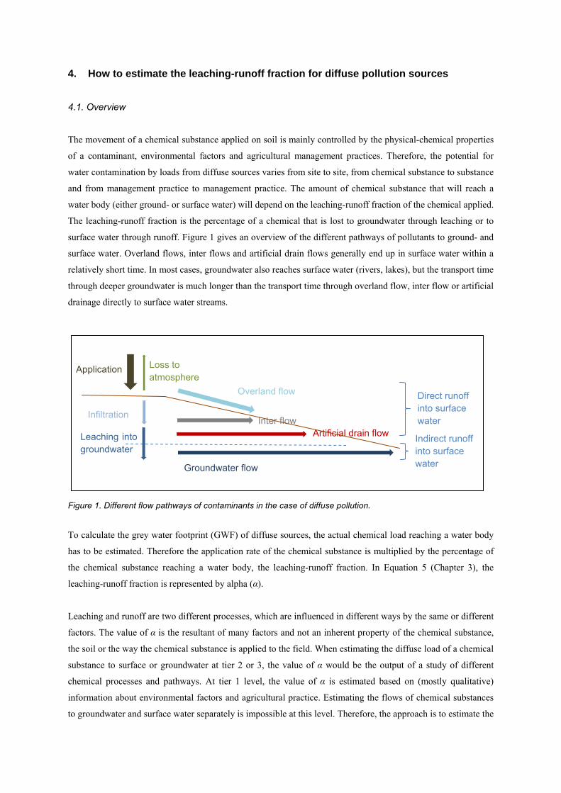
The leaching-runoff fraction is the percentage of a chemical that is lost to groundwater through leaching or to
surface water through runoff. Figure 1 gives an overview of the different pathways of pollutants to ground- and
surface water. Overland flows, inter flows and artificial drain flows generally end up in surface water within a
relatively short time. In most cases, groundwater also reaches surface water (rivers, lakes), but the transport time
through deeper groundwater is much longer than the transport time through overland flow, inter flow or artificial
drainage directly to surface water streams.
Figure 1. Different flow pathways of contaminants in the case of diffuse pollution.
To calculate the grey water footprint (GWF) of diffuse sources, the actual chemical load reaching a water body
has to be estimated. Therefore the application rate of the chemical substance is multiplied by the percentage of
the chemical substance reaching a water body, the leaching-runoff fraction. In Equation 5 (Chapter 3), the
leaching-runoff fraction is represented by alpha (α).
Leaching and runoff are two different processes, which are influenced in different ways by the same or different
factors. The value of α is the resultant of many factors and not an inherent property of the chemical substance,
the soil or the way the chemical substance is applied to the field. When estimating the diffuse load of a chemical
substance to surface or groundwater at tier 2 or 3, the value of α would be the output of a study of different
chemical processes and pathways. At tier 1 level, the value of α is estimated based on (mostly qualitative)
information about environmental factors and agricultural practice. Estimating the flows of chemical substances
to groundwater and surface water separately is impossible at this level. Therefore, the approach is to estimate the
Loss to atmosphere
Overland flow
Infiltration
Groundwater flow
Direct runoff into surface water
Artificial drain flow
Application
Inter flow
Leaching into groundwater
Indirect runoff into surface water
16 / Grey water footprint accounting: Tier1 supporting guidelines
overall leaching-runoff fraction, without making explicit which part refers to the leaching to groundwater and
which part to the direct runoff to surface water. More advanced methods should be used if a differentiation is to
be made.
These guidelines suggest default global average leaching-runoff fractions that can be used if no local
information is available, which may occur for example when companies aim to assess the GWF of their supply
chain without knowing the precise origin of inputs. With some local information, one can make more site-
specific estimates of leaching-runoff fractions. There are three categories of influencing factors, which should
be considered to estimate the leaching-runoff fraction at tier 1 level:
physical-chemical properties of the chemical substance applied (like the soil-water partition coefficient Kd or
the soil organic carbon-water partition coefficient Koc, and the persistency of the substance);
environmental conditions (like soil properties and climatic conditions); and
management practices (like the application rate of the chemical substance, the harvest, the presence of
artificial drainage).
In each category, there are different specific factors that influence the leaching-runoff fraction. The list of
influencing factors is slightly different per chemical substance group: nutrients, metals, and pesticides, whereby
nutrients are further distinguished into nitrogen and phosphorus. Sections 4.2 to 4.5 describe the influencing
factors per type of chemical substance.
The state of a factor determines whether the leaching-runoff potential for a chemical substance will be relatively
low or high. For nitrogen, for example, soils with little water retention, such as sandy soils, generally have
higher leaching (Simmelsgaard, 1998). Per factor i, a certain score s between 0 and 1 for the leaching-runoff
potential will be given, based on the state of the factor. A score of 0 means a very low leaching-runoff potential,
a score 0.33 a low, a score 0.67 a high, and a score of 1 a very high leaching-runoff potential. If no information
about the state of a factor can be obtained, it is suggested to use a score of 0.5 for the corresponding factor.
Each separate factor will influence the leaching-runoff of a chemical substance to a greater or lesser extent.
Therefore, weights are given for each factor. A weight w per factor i denotes the importance of the factor. The
weights given to the separate influencing factors add up to a total of 100. Tables 3-6 in Sections 4.2 to 4.5 show,
per type of chemical substance, the weight per influencing factor and what is the score per factor depending on
the state of the factor. The supporting information and maps in Appendices I-II may help to estimate the state of
a certain influencing factor if no local data is available.
Once the state of each factor has been determined, the leaching-runoff fraction α can be calculated using the
following equation:
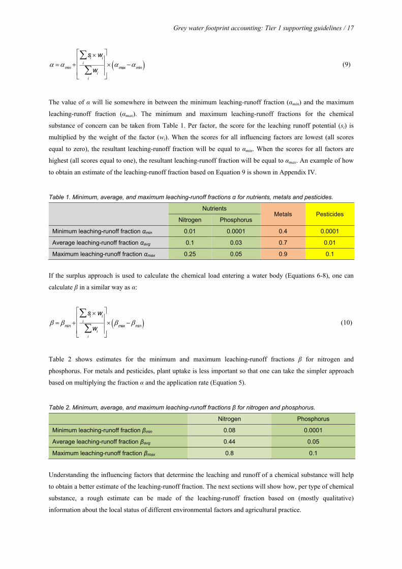
Grey water footprint accounting: Tier 1 supporting guidelines / 17
min
siw
ii
w
ii
max
min (9)
The value of α will lie somewhere in between the minimum leaching-runoff fraction (αmin) and the maximum
leaching-runoff fraction (αmax). The minimum and maximum leaching-runoff fractions for the chemical
substance of concern can be taken from Table 1. Per factor, the score for the leaching runoff potential (si) is
multiplied by the weight of the factor (wi). When the scores for all influencing factors are lowest (all scores
equal to zero), the resultant leaching-runoff fraction will be equal to αmin. When the scores for all factors are
highest (all scores equal to one), the resultant leaching-runoff fraction will be equal to αmax. An example of how
to obtain an estimate of the leaching-runoff fraction based on Equation 9 is shown in Appendix IV.
Table 1. Minimum, average, and maximum leaching-runoff fractions α for nutrients, metals and pesticides.
Nutrients Metals Pesticides
Nitrogen Phosphorus
Minimum leaching-runoff fraction αmin 0.01 0.0001 0.4 0.0001
Average leaching-runoff fraction αavg 0.1 0.03 0.7 0.01
Maximum leaching-runoff fraction αmax 0.25 0.05 0.9 0.1
If the surplus approach is used to calculate the chemical load entering a water body (Equations 6-8), one can
calculate β in a similar way as α:
min
s
iw
ii
w
ii
max
min (10)
Table 2 shows estimates for the minimum and maximum leaching-runoff fractions β for nitrogen and
phosphorus. For metals and pesticides, plant uptake is less important so that one can take the simpler approach
based on multiplying the fraction α and the application rate (Equation 5).
Table 2. Minimum, average, and maximum leaching-runoff fractions β for nitrogen and phosphorus.
Nitrogen Phosphorus
Minimum leaching-runoff fraction βmin 0.08 0.0001
Average leaching-runoff fraction βavg 0.44 0.05
Maximum leaching-runoff fraction βmax 0.8 0.1
Understanding the influencing factors that determine the leaching and runoff of a chemical substance will help
to obtain a better estimate of the leaching-runoff fraction. The next sections will show how, per type of chemical
substance, a rough estimate can be made of the leaching-runoff fraction based on (mostly qualitative)
information about the local status of different environmental factors and agricultural practice.
18 / Grey water footprint accounting: Tier1 supporting guidelines
4.2. Nitrogen
Nitrogen is one of the most important plant nutrients and forms one of the most mobile compounds in the soil-
crop system (National Research Council, 1993). Nitrogen is added to the soil in the form of nitrate (NO3) or
ammonium (NH4) in artificial fertilizer, as well as in the form of organic nitrogen and ammonia in different
types of manure. In most soils, ammonium and organic nitrogen transform to nitrate over time. Nitrogen fixation
and deposition are also important nitrogen inputs into the soil. Nitrogen fixation refers to the conversion of
atmospheric nitrogen (the gas N2) into ammonium (NH4) by bacteria living symbiotically in the roots of
leguminous crops. Deposition refers to nitrogen compounds that are emitted from industry, traffic and
agriculture and return to the soil via dry and wet deposition. Especially nitrogen fixation can be a major input
depending on the crop grown (leguminous crops fix nitrogen and after harvest the leaching can be substantial)
and the fertilization level (high level of fertilization generally reduces fixation).
The leaching-runoff of nitrogen to the combined ground-surface water system can be estimated in four different
ways, listed from least to most preferred, but also from least to most data-demanding:
1. based on the N-application rate (Equation 5) and the global average value for the leaching-runoff fraction α
(Table 1).
2. based on the N-surplus in the soil (Equations 6-8) and the global average value for the leaching-runoff
fraction β (Table 2).
3. based on the N-application rate (Equation 5), a rough estimate of the leaching-runoff fraction α (Equation 9)
within the range of αmin and αmax (Table 1) and the estimated nitrogen leaching-runoff potential (Table 3).
4. based on the N-surplus in the soil (Equations 6-8), a rough estimate of the leaching-runoff fraction β
(Equation 10) within the range of βmin and βmax (Table 2) and the estimated nitrogen leaching-runoff potential
(Table 3).
The first two calculation methods are simplest, since no local data on soil and climate conditions or agricultural
practice are required. However, the outcome will not depend on local factors, while in reality leaching-runoff
fractions can vary over a wide range, depending on local conditions. The last two calculation methods are better
because they take into account local factors, even though mostly in a qualitative way. The method based on
nitrogen surplus is more precise than the method based on the nitrogen application rate. The nitrogen contained
in harvested crops represents the greatest and most important output of nitrogen from croplands. The amount of
nitrogen taken up varies depending on the crop and yield. Therefore, it is best to subtract the nitrogen offtake
due to harvest from the nitrogen application rate before estimating the amount of nitrogen leaching or running
off. The nitrogen surplus is the difference between the amount of nitrogen applied and the amount of nitrogen
taken up by the crop and harvested. The nitrogen surplus should be estimated using primarily local data.
Alternatively, yields can be obtained from national and global statistical databases. N-content in crops can be
found in agricultural handbooks and databases, such as listed for example in Appendix I under the heading
‘nutrient surplus’.
Grey water footprint accounting: Tier 1 supporting guidelines / 19
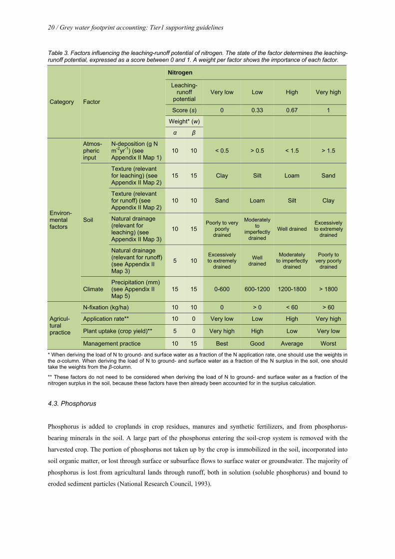
In the case of nitrogen, leaching and runoff is mainly influenced by:
environmental factors: N-deposition, soil properties (texture, drainage) and climate (precipitation); and
agricultural practice: N-fixation, N-application rate, N-offtake through harvest and management practice.
Table 3 can be used to estimate the leaching-runoff potential in a specific location. The table helps to identify
the leaching-runoff potential (from very low to very high, with scores from 0 to 1) per influencing factor. The
table further shows the importance (weight) per influencing factor. When determining the scores for the
leaching-runoff potential per influencing factor, it is generally better to use local data on these factors. If no
local data are available, one can choose to derive data from global databases or literature. A few relevant
references and maps are provided in Appendix II. For those influencing factors for which no information can be
obtained, it is suggested to use a score of 0.5.
The different factors influence the leaching-runoff fraction as follows:
N-deposition will considerably influence the amount of nitrogen that will leach or run off. The higher the N-
deposition, the higher the leaching-runoff potential.
Regarding soil texture, sandy soils are particularly vulnerable to nitrate leaching because of their low water
holding capacity, whereas loamy, silty and clayey soils retain water, and with it nitrogen, more effectively,
thus lowering leaching capacity. Losses through runoff are influenced by soil texture opposite to leaching.
The poorer natural drainage of a soil, the less nitrogen will leach to groundwater, but the higher the
probability of runoff towards surface water.
Rainfall is probably the most important climate factor affecting nitrate leaching and runoff. Heavy rain
causes a peak in leaching and runoff, because water flushes nitrate from soil.
The amount of nitrogen lost through leaching or runoff is related to the amount of nitrogen applied. The
higher the application rate, the larger the fraction of loss.
Depending on the crop grown (and the associated nitrogen uptake) and the yield, the amount of nitrogen
exposed to leaching and runoff will differ. The higher the plant uptake and crop yield, the lower the potential
of leaching and runoff.
Management practices such as timing and mode of nitrogen application can affect chemical and transport
processes in the soil. Excessive irrigation increases the risk of nitrate leaching (Thompson et al., 2007). Best
management practice is highly specific to crop and location (National Research Council, 1993). Here we
categorize management practice from ‘best’ to ‘worst’. ‘Best’ includes a series of measures reducing the risk
of leaching-runoff. In order to classify the management practice in a particular situation, the questionnaire
provided in Appendix III can be used as a reference. If no information on management practice is available,
we suggest using ‘best’ or ‘good’ for industrialized countries, ‘good’ or ‘average’ for emerging countries and
‘average’ or ‘worst’ for developing countries.
20 / Grey water footprint accounting: Tier1 supporting guidelines
Table 3. Factors influencing the leaching-runoff potential of nitrogen. The state of the factor determines the leaching-runoff potential, expressed as a score between 0 and 1. A weight per factor shows the importance of each factor.
Category Factor
Nitrogen
Leaching-runoff
potential Very low Low High Very high
Score (s) 0 0.33 0.67 1
Weight* (w)
α β
Environ-mental factors
Atmos-pheric input
N-deposition (g N m-2yr-1) (see Appendix II Map 1)
10 10 < 0.5 > 0.5 < 1.5 > 1.5
Soil
Texture (relevant for leaching) (see Appendix II Map 2)
15 15 Clay Silt Loam Sand
Texture (relevant for runoff) (see Appendix II Map 2)
10 10 Sand Loam Silt Clay
Natural drainage (relevant for leaching) (see Appendix II Map 3)
10 15 Poorly to very
poorly drained
Moderately to
imperfectly drained
Well drained Excessively to extremely
drained
Natural drainage (relevant for runoff) (see Appendix II Map 3)
5 10 Excessively to extremely
drained
Well drained
Moderately to imperfectly
drained
Poorly to very poorly
drained
Climate Precipitation (mm) (see Appendix II Map 5)
15 15 0-600 600-1200 1200-1800 > 1800
Agricul-tural practice
N-fixation (kg/ha) 10 10 0 > 0 < 60 > 60
Application rate** 10 0 Very low Low High Very high
Plant uptake (crop yield)** 5 0 Very high High Low Very low
Management practice 10 15 Best Good Average Worst
* When deriving the load of N to ground- and surface water as a fraction of the N application rate, one should use the weights in the α-column. When deriving the load of N to ground- and surface water as a fraction of the N surplus in the soil, one should take the weights from the β-column.
** These factors do not need to be considered when deriving the load of N to ground- and surface water as a fraction of the nitrogen surplus in the soil, because these factors have then already been accounted for in the surplus calculation.
4.3. Phosphorus
Phosphorus is added to croplands in crop residues, manures and synthetic fertilizers, and from phosphorus-
bearing minerals in the soil. A large part of the phosphorus entering the soil-crop system is removed with the
harvested crop. The portion of phosphorus not taken up by the crop is immobilized in the soil, incorporated into
soil organic matter, or lost through surface or subsurface flows to surface water or groundwater. The majority of
phosphorus is lost from agricultural lands through runoff, both in solution (soluble phosphorus) and bound to
eroded sediment particles (National Research Council, 1993).
Grey water footprint accounting: Tier 1 supporting guidelines / 21
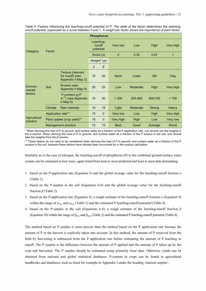
Table 4. Factors influencing the leaching-runoff potential of P. The state of the factor determines the leaching-runoff potential, expressed as a score between 0 and 1. A weight per factor shows the importance of each factor.
Category Factor
Phosphorus
Leaching-runoff
potential Very low Low High Very high
Score (s) 0 0.33 0.67 1
Weight* (w)
α β
Environ- mental factors
Soil
Texture (relevant for runoff) (see Appendix II Map 2)
15 25 Sand Loam Silt Clay
Erosion (see Appendix II Map 9)
20 25 Low Moderate High Very high
P-content (g P m−2) (see Appendix II Map 6)
15 20 < 200 200-400 400-700 > 700
Climate Rain intensity 10 15 Light Moderate Strong Heavy
Agricultural practice
Application rate** 15 0 Very low Low High Very high
Plant uptake (crop yield)** 10 0 Very high High Low Very low
Management practice 15 15 Best Good Average Worst
* When deriving the load of P to ground- and surface water as a fraction of the P application rate, one should use the weights in the α-column. When deriving the load of P to ground- and surface water as a fraction of the P surplus in the soil, one should take the weights from the β-column.
** These factors do not need to be considered when deriving the load of P to ground- and surface water as a fraction of the P surplus in the soil, because these factors have already been accounted for in the surplus calculation.
Similarly as in the case of nitrogen, the leaching-runoff of phosphorus (P) to the combined ground-surface water
system can be estimated in four ways, again listed from least to most preferred and least to most data-demanding:
1. based on the P-application rate (Equation 5) and the global average value for the leaching-runoff fraction α
(Table 1).
2. based on the P-surplus in the soil (Equations 6-8) and the global average value for the leaching-runoff
fraction β (Table 2).
3. based on the P-application rate (Equation 5), a rough estimate of the leaching-runoff fraction α (Equation 9)
within the range of αmin and αmax (Table 1) and the estimated P leaching-runoff potential (Table 4).
4. based on the P-surplus in the soil (Equations 6-8), a rough estimate of the leaching-runoff fraction β
(Equation 10) within the range of βmin and βmax (Table 2) and the estimated P leaching-runoff potential (Table 4).
The method based on P surplus is more precise than the method based on the P application rate because the
amount of P in the harvest is explicitly taken into account. In this method, the amount of P removed from the
field by harvesting is subtracted from the P application rate before estimating the amount of P leaching or
runoff. The P surplus is the difference between the amount of P applied and the amount of P taken up by the
crop and harvested. The P surplus should be estimated using primarily local data. Otherwise yields can be
obtained from national and global statistical databases. P-content in crops can be found in agricultural
handbooks and databases, such as listed for example in Appendix I under the heading ‘nutrient surplus’.
22 / Grey water footprint accounting: Tier1 supporting guidelines
The leaching-runoff potential for phosphorus is mainly influenced by:
environmental factors: soil (texture, erosion, P-content) and climate (rain intensity);
agricultural practice: P-application rate, P-offtake through harvest and management practice.
The leaching-runoff potential in a specific location can be estimated with Table 4, which helps to identify the
leaching-runoff potential (from very low to very high, with scores from 0 to 1) per influencing factor. The table
further shows the importance (weight) per influencing factor. When determining the leaching-runoff potential
per factor, it is generally better to use local data. If no local data are available, one can choose to derive data
from global databases or literature. A few relevant references and maps are provided in Appendix II. For those
influencing factors for which no information can be obtained, it is suggested to use a score of 0.5.
The different factors influence the leaching-runoff fraction as follows:
Regarding soil texture, clayey and silty soils generally have low infiltration rates and therefore more surface
runoff and erosion. These soils are therefore particularly vulnerable to surface runoff of P, whereas loamy
and sandy soils have higher infiltration, allowing P to be sorbed in the soil column.
Soil erosion contributes significantly to the inputs of P into surface water bodies. One can apply the
Universal Soil Loss Equation (Wischmeier and Smith, 1978) as a simple equation that attempts to predict the
annual average erosion rate through factors describing the rainfall (erosivity, which depends on rainfall
energy and intensity), soil (erodibility, which depends on soil texture, structure, organic matter content and
permeability), slope and slope length, the vegetation and soil conservation practices. The equation allows
also inclusion of modifying factors for vegetation and agricultural practices.
Increased residual P levels in the soil lead to increased phosphorus loadings to surface water, both in
solution and attached to soil particles (National Research Council, 1993). Therefore, the P content in the soil
is a critical factor in determining actual loads of P to surface water.
The higher rain intensities, the higher the probability that P will be transported through overland flow to
surface water, either dissolved or with eroded soil.
The lower the P-application rate, the lower the risk of leaching or runoff.
Depending on the crop grown (and the associated P uptake) and the yield, the amount of P exposed to
leaching and runoff will differ. The higher the plant uptake and crop yield, the lower the leaching-runoff
potential.
Best management practice includes a series of measures reducing the risk of leaching-runoff. In order to
classify the management practice in a particular situation, the questionnaire provided in Appendix III can be
used as a reference. If no information on management practice is available, we suggest using ‘best’ or ‘good’
for industrialized countries, ‘good’ or ‘average’ for emerging countries and ‘average’ or ‘worst’ for
developing countries.
Grey water footprint accounting: Tier 1 supporting guidelines / 23
4.4. Metals
All soils naturally contain trace levels of metals, which are primarily related to the geology of the region. Metals
added to soil will normally be retained at the soil surface. An important parameter is the so-called distribution
coefficient Kd, also called the soil-water partition coefficient. The Kd is expressed in L/kg and defined as the
ratio of a chemical's sorbed concentration (mg/kg) to the dissolved concentration (mg/L) at equilibrium. Metals
associated with the aqueous phase of soils are subject to movement with soil water, and may be transported to
ground water (McLean and Bledsoe, 1992). Most of metal losses, though, are through lateral movement of soil,
due to mechanical operations or erosion (Camobreco et al., 1996). Metals, unlike organic chemicals, cannot be
degraded. Therefore, sooner or later, metals applied onto the soil will reach a water body either through
leaching, runoff or erosion.
Because of the wide range of soil characteristics and various forms by which metals can be added to soil,
evaluating the extent of metal retention by a soil is site specific (McLean and Bledsoe, 1992). Changes in the
soil environment over time, such as the degradation of organic waste, changes in pH, redox potential, or soil
solution composition, due to various remediation schemes or to natural weathering processes may enhance metal
mobility. Therefore, field specific models for evaluating the behaviour of metals in soils should be used. Here
we attempt to establish a simplified tier 1 approach to estimate the leaching-runoff potential of applied metals to
soil, which should only be used if no better method is available.
The leaching-runoff of metals to the combined ground-surface water system can be estimated by multiplying the
metal-application rate with the leaching-runoff fraction α (Equation 5). If no local data are available, one can
assume the global average value for the leaching-runoff fraction α (Table 1). More precise, but requiring some
local data, is to make a rough estimate of the leaching-runoff fraction α (Equation 9) within the range of αmin and
αmax (Table 1) and the estimated metal leaching-runoff potential (Table 5).
The leaching-runoff potential of metals is mainly influenced by:
the soil-water partition coefficient Kd (which depends on the chemical properties of the metal, but
environmental conditions such as pH as well);
environmental factors (beside the environmental factors that influence the Kd value): soil properties (texture,
erosion potential) and climate (rain intensity);
site management: artificial drainage.
The leaching-runoff potential in a specific location can be estimated with Table 5, which helps to identify the
leaching-runoff potential (from very low to very high, with scores from 0 to 1) per influencing factor. The table
further shows the importance (weight) per influencing factor. When determining the leaching-runoff potential
per factor, it is generally better to use local data. If no local data are available, one can choose to derive data
from global databases or literature. A few relevant references and maps are provided in Appendices I-II. For
those influencing factors for which no information can be obtained, it is suggested to use a score of 0.5.
24 / Grey water footprint accounting: Tier1 supporting guidelines
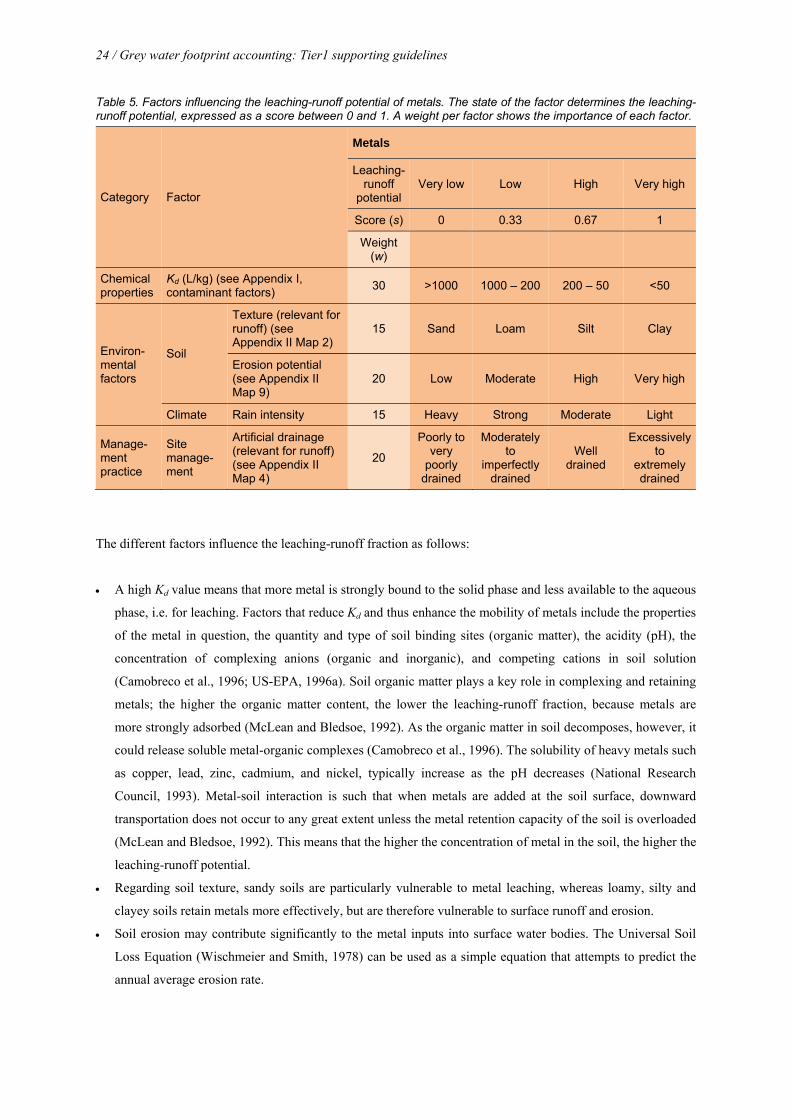
Table 5. Factors influencing the leaching-runoff potential of metals. The state of the factor determines the leaching-runoff potential, expressed as a score between 0 and 1. A weight per factor shows the importance of each factor.
Category Factor
Metals
Leaching-runoff
potential Very low Low High Very high
Score (s) 0 0.33 0.67 1
Weight (w)
Chemical properties
Kd (L/kg) (see Appendix I, contaminant factors)
30 >1000 1000 – 200 200 – 50 <50
Environ- mental factors
Soil
Texture (relevant for runoff) (see Appendix II Map 2)
15 Sand Loam Silt Clay
Erosion potential (see Appendix II Map 9)
20 Low Moderate High Very high
Climate Rain intensity 15 Heavy Strong Moderate Light
Manage-ment practice
Site manage-ment
Artificial drainage (relevant for runoff) (see Appendix II Map 4)
20
Poorly to very
poorly drained
Moderately to
imperfectly drained
Well drained
Excessively to
extremely drained
The different factors influence the leaching-runoff fraction as follows:
A high Kd value means that more metal is strongly bound to the solid phase and less available to the aqueous
phase, i.e. for leaching. Factors that reduce Kd and thus enhance the mobility of metals include the properties
of the metal in question, the quantity and type of soil binding sites (organic matter), the acidity (pH), the
concentration of complexing anions (organic and inorganic), and competing cations in soil solution
(Camobreco et al., 1996; US-EPA, 1996a). Soil organic matter plays a key role in complexing and retaining
metals; the higher the organic matter content, the lower the leaching-runoff fraction, because metals are
more strongly adsorbed (McLean and Bledsoe, 1992). As the organic matter in soil decomposes, however, it
could release soluble metal-organic complexes (Camobreco et al., 1996). The solubility of heavy metals such
as copper, lead, zinc, cadmium, and nickel, typically increase as the pH decreases (National Research
Council, 1993). Metal-soil interaction is such that when metals are added at the soil surface, downward
transportation does not occur to any great extent unless the metal retention capacity of the soil is overloaded
(McLean and Bledsoe, 1992). This means that the higher the concentration of metal in the soil, the higher the
leaching-runoff potential.
Regarding soil texture, sandy soils are particularly vulnerable to metal leaching, whereas loamy, silty and
clayey soils retain metals more effectively, but are therefore vulnerable to surface runoff and erosion.
Soil erosion may contribute significantly to the metal inputs into surface water bodies. The Universal Soil
Loss Equation (Wischmeier and Smith, 1978) can be used as a simple equation that attempts to predict the
annual average erosion rate.
Grey water footprint accounting: Tier 1 supporting guidelines / 25
The higher rainfall intensities, the higher the probability that metals will be washed out or that the soil
erodes, taking along the metals contained in the soil.
Artificial drainage increases the probability that metals end up in surface water. Soils that are poorly drained
will accumulate the metals; in this case, metals can, in the long term, reach groundwater through leaching or
surface water through erosion.
4.5. Pesticides
Leaching and runoff of pesticides is strongly influenced by their specific chemical properties. The term
pesticides includes different chemical mixtures with different purposes (insecticides, herbicides, fungicides,
etc.). They usually include one or more ‘active ingredients’ (specific chemical substances), with different
properties and behaviours. Estimating the leaching and runoff potential for all of these compounds is
challenging. In addition, technical difficulties and the high costs associated with measuring the fraction of
pesticides present in the various compartments over time make a full understanding of the fate and transport of
pesticides more difficult (National Research Council, 1993).
The leaching-runoff of pesticides to the combined ground-surface water system can be estimated by multiplying
the pesticide-application rate with the leaching-runoff fraction α (Equation 5). If no local data are available, one
can assume the global average value for the leaching-runoff fraction α (Table 1). More precise, but requiring
some local data, is to make a rough estimate of the leaching-runoff fraction α (Equation 9) within the range of
αmin and αmax (Table 1) and the estimated metal leaching-runoff potential (Table 6).
The leaching-runoff potential of pesticides is mainly influenced by:
pesticide properties: the soil organic carbon-water partitioning coefficient (Koc) and persistence (half-life);
environmental factors: soil properties (soil texture, organic matter content) and climate (rain intensity,
precipitation);
agricultural practice.
The leaching-runoff potential of pesticides in a specific location can be estimated with Table 6, which helps to
identify the leaching-runoff potential (from very low to very high, with scores from 0 to 1) per influencing
factor. The table further shows the importance (weight) per influencing factor. When determining the leaching-
runoff potential per factor, it is generally better to use local data. If no local data are available, one can choose to
derive data from global databases or literature. A few relevant references and maps are provided in Appendices
I-II. For those influencing factors for which no information can be obtained, it is suggested to use a score of 0.5.
26 / Grey water footprint accounting: Tier1 supporting guidelines
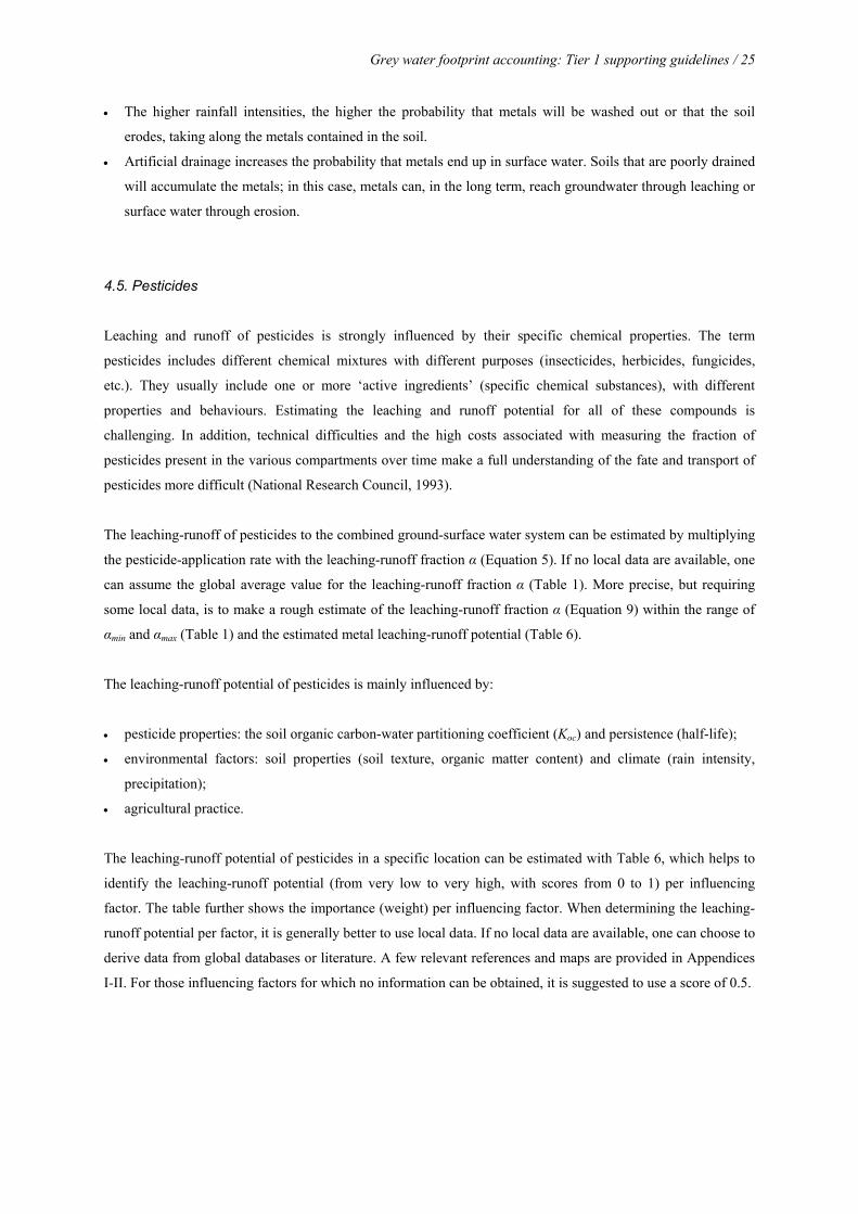
Table 6. Factors influencing the leaching-runoff potential of pesticides. The state of the factor determines the leaching-runoff potential, expressed as a score between 0 and 1. A weight per factor shows the importance of each factor.
Category Factor
Pesticides
Leaching-runoff
potential Very low Low High Very high
Score (s) 0 0.33 0.67 1
Weight (w)
Chemical properties
Koc (L/kg) (see Appendix I, contaminant factors)
20 >1000 1000 - 200 200 - 50 <50
Persistence (half-life in days) (relevant for leaching) (see Appendix I, contaminant factors)
15 <10 10 - 30 30 - 100 >100
Persistence (half-life in days) (relevant for runoff) (see Appendix I, contaminant factors)
10 <10 10 - 30 30 - 100 >100
Environmental factors
Soil
Texture (relevant for leaching) (see Appendix II Map 2)
15 Clay Silt Loam Sand
Texture (relevant for runoff) (see Appendix II Map 2)
10 Sand Loam Silt Clay
Organic matter content (kg/m2) (see Appendix II Map 8)
10 >80 41 - 80 21 - 40 <20
Climate
Rain intensity (relevant for runoff)
5 Light Moderate Strong Heavy
Precipitation (mm) (relevant for leaching) (see Appendix II Map 5)
5 0-600 600-1200 1200-1800
> 1800
Agricultural practice
Management practice (relevant for runoff)
10 Best Good Average Worst
The different factors influence the leaching-runoff fraction as follows:
The soil organic carbon-water partitioning coefficient (Koc) is the ratio of the mass of a chemical that is
adsorbed in the soil per unit mass of organic carbon in the soil to the equilibrium concentration of the
chemical in solution. It is the soil-water partition coefficient (Kd) normalized to total organic carbon content.
Koc values are useful in predicting the mobility of organic soil contaminants: the lower the Koc value, the
lower the adsorption affinity of a chemical, the higher the leaching-runoff potential.
The persistence of an active ingredient of a pesticide is commonly evaluated in terms of half-life, which is
the time that it takes for 50 per cent of a chemical substance to be degraded or transformed. Pesticides with a
long half-life are more persistent and therefore have a higher leaching-runoff potential (National Research
Council, 1993).
The soil texture is an important factor, because the texture determines the movement of water, which in turn
determines the movement of the pesticides dissolved in water. While leaching generally increases from
clayey to sandy soils, runoff decreases.
Grey water footprint accounting: Tier 1 supporting guidelines / 27
The organic matter content in the soil will influence the biodegradability of the active ingredients of a
pesticide. The organic matter content is an important variable affecting sorption of the active ingredients
onto soil particles. Adsorption retains chemical substances in the soil, thus allowing more time for
degradation by chemical and biological processes. Organic matter provides binding sites and is very reactive
chemically. Soil organic matter also influences how much water the soil can hold before movement occurs.
Increasing organic matter will increase the water-holding capacity of the soil (USDA, 1997).
The more intense the rainfall, the higher the probability that pesticides will be washed out or that the soil
erodes.
At large rainfall rates, it is likely that more pesticides will reach the groundwater through leaching.
Additionally, there is a greater potential that a rainfall event will closely follow application, which can be an
important factor in pesticide runoff.
Management practices such as the mode of pesticide application affect the amount reaching freshwater
bodies. Spraying, for instance, may lead to drift away from the field, and spraying to close by streams will
increase the risk of pesticides depositing directly onto the water. Best management practice includes a series
of measures reducing the risk of leaching-runoff. In order to classify the management practice in a particular
situation, the questionnaire provided in Appendix III can be used as a reference. If no information on
management practice is available, we suggest using ‘best’ or ‘good’ for industrialized countries, ‘good’ or
‘average’ for emerging countries and ‘average’ or ‘worst’ for developing countries.

5. Which maximum allowable concentration to use
5.1. Introduction
Grey water footprint (GWF) calculations are carried out using ambient water quality standards for the receiving
freshwater body (in other words, standards with respect to maximum allowable concentrations). The reason is
that the GWF aims to show the required ambient water volume to assimilate chemical substances. For a
particular chemical substance, the ambient water quality standard may vary from one to another water body.
Besides, the natural concentration may vary from place to place. As a result, a certain pollutant load can result in
one GWF in one place and another GWF in another place. This is reasonable, because the required water
volume for assimilating a certain pollutant load will indeed be different depending on the difference between the
maximum allowable and the natural concentration (Hoekstra et al., 2011).
Although ambient water quality standards often exist in national or state legislation or have to be formulated by
catchment and/or water body in the framework of national legislation or by regional agreement (like in the
European Water Framework Directive), they do not exist for all chemical substances and all places (Hoekstra et
al., 2011). This is why, if no local information can be obtained, this guideline proposes to use the maximum
allowable concentrations as based on the assessment of long term/chronic environmental effects from one of
these sources:
EU (2013) – European priority substances in the field of water policy.
US-EPA (2013) – US National Recommended Water Quality Criteria - Aquatic Life Criteria.
CCME (2013) - Canadian Water Quality Guidelines for the Protection of Aquatic Life.
These sources are recommended because the water quality standards included in these references are among the
most advanced and they include relatively large sets of parameters1. They have large application areas as well
and are referenced by many countries that establish country-specific standards.
In the following sections, maximum allowable concentrations are suggested for the GWF calculation for the
case in which no local standards are available. Separate tables are included for four groups of parameters:
nutrients, metals & inorganics, pesticides & organics and ‘other water quality parameters’. Per chemical
substance, it is recommended to select the strictest standard from the above three sources. For cross-country
studies, it is recommended to use a consistent set of standards, so that differences in national legislations will
not affect the GWF calculations. In any case, it is recommended to explicitly mention the standards used.
1 EC (2008) includes about 35 parameters, US-EPA (2013) 60 parameters and CCME (2013) 125 parameters.
30 / Grey water footprint accounting: Tier1 supporting guidelines
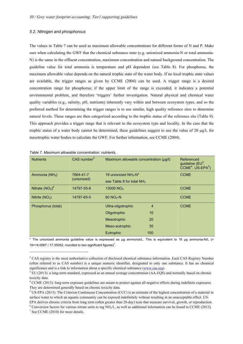
5.2. Nitrogen and phosphorous
The values in Table 7 can be used as maximum allowable concentrations for different forms of N and P. Make
sure when calculating the GWF that the chemical substance state (e.g. unionized ammonia-N or total ammonia-
N) is the same in the effluent concentration, maximum concentration and natural background concentration. The
guideline value for total ammonia is temperature and pH dependent (see Table 8). For phosphorus, the
maximum allowable value depends on the natural trophic state of the water body. If no local trophic state values
are available, the trigger ranges as given by CCME (2004) can be used. A trigger range is a desired
concentration range for phosphorus; if the upper limit of the range is exceeded, it indicates a potential
environmental problem, and therefore ‘triggers’ further investigation. Natural physical and chemical water
quality variables (e.g., salinity, pH, nutrients) inherently vary within and between ecosystem types, and so the
preferred method for determining the trigger ranges is to use similar, high quality reference sites to determine
natural levels. These ranges are then categorized according to the trophic status of the reference site (Table 9).
This approach provides a trigger range that is relevant to the ecosystem type and locality. In the case that the
trophic status of a water body cannot be determined, these guidelines suggest to use the value of 20 µg/L for
mesotrophic water bodies to calculate the GWF. For further information, see CCME (2004).
Table 7. Maximum allowable concentration: nutrients.
Nutrients CAS number2 Maximum allowable concentration (µg/l) Referenced guideline (EU3, CCME4, US-EPA5)
Ammonia (NH3) 7664-41-7 (unionized)
19 unionized NH3-N*
see Table 8 for total NH3
CCME
Nitrate (NO3)6 14797-55-8 13000 NO3 CCME
Nitrite (NO2) 14797-65-0 60 NO2-N CCME
Phosphorus (total) Ultra-oligotrophic 4
Oligotrophic 10
Mesotrophic 20
Meso-eutrophic 35
Eutrophic 100
CCME
* The unionized ammonia guideline value is expressed as μg ammonia/L. This is equivalent to 16 μg ammonia-N/L (=
19×14.0067 / 17.35052, rounded to two significant figures)7.
2 CAS registry is the most authoritative collection of disclosed chemical substance information. Each CAS Registry Number (often referred to as CAS number) is a unique numeric identifier, designated to only one substance. It has no chemical significance and is a link to information about a specific chemical substance (www.cas.org). 3 EU (2013): a long-term standard, expressed as an annual average concentration (AA-EQS) and normally based on chronic toxicity data. 4 CCME (2013): long-term exposure guidelines are meant to protect against all negative effects during indefinite exposures. They are determined generally based on chronic toxicity data. 5 US-EPA (2013): The Criterion Continuous Concentration (CCC) is an estimate of the highest concentration of a material in surface water to which an aquatic community can be exposed indefinitely without resulting in an unacceptable effect. US-EPA derives chronic criteria from long term (often greater than 28-day) tests that measure survival, growth, or reproduction. 6 Conversion factors for various nitrate units to mg NO3/L, as well as additional information can be found in CCME (2012). 7 See CCME (2010) for more details.
Grey water footprint accounting: Tier 1 supporting guidelines / 31
Table 8. Water quality guidelines for total ammonia for the protection of aquatic life (mg NH3/L). Source: CCME (2010).
Temperature (oC) pH
6.0 6.5 7.0 7.5 8.0 8.5 9.0 10.0
0 231 73.0 23.1 7.32 2.33 0.749 0.25 0.042
5 153 48.3 15.3 4.84 1.54 0.502 0.172 0.034
10 102 32.4 10.3 3.26 1.04 0.343 0.121 0.029
15 69.7 22.0 6.98 2.22 0.715 0.239 0.089 0.026
20 48.0 15.2 4.82 1.54 0.499 0.171 0.067 0.024
25 33.5 10.6 3.37 1.08 0.354 0.125 0.053 0.022
30 23.7 7.50 2.39 0.767 0.256 0.094 0.043 0.021
Measurements of total ammonia in the aquatic environment are often expressed as mg/L total ammonia-N. The present guideline values (in mg/L NH3) can be converted to mg/L total ammonia-N by multiplying the guideline values by 0.8224.
Table 9. Total phosphorus trigger ranges. Source: CCME (2004).
Trophic status Canadian trigger ranges total phosphorus (μg/L)
Ultra-oligotrophic < 4
Oligotrophic 4-10
Mesotrophic 10-20
Meso-eutrophic 20-35
Eutrophic 35-100
Hyper-eutrophic > 100
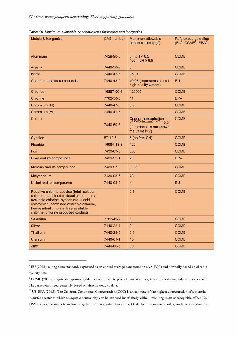
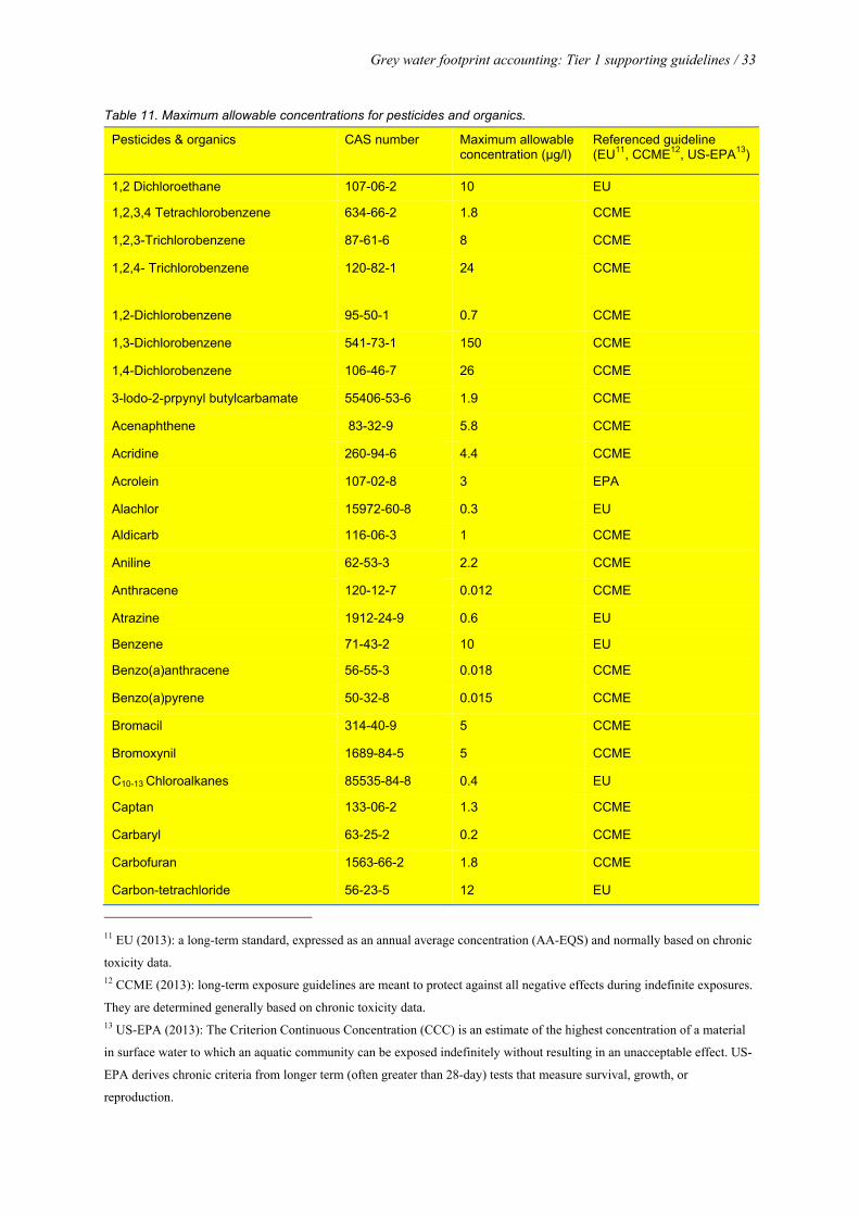
5.3. Metals & inorganics, pesticides & organics, and additional water quality parameters
Tables 10-11 show suggested maximum allowable concentrations for metals/inorganics and pesticides/organics,
respectively, for those cases where no local standards are available or for comparative studies. There are some
water quality parameters, which are neither listed in the EU standard as priority substances, nor in the CCME
and US-EPA guidelines, but are often used by industry to assess their water quality limits. Therefore, if no local
standards are available, these guidelines suggest using the values from EEC (1975) concerning the quality
required of surface water intended for the abstraction of drinking water (Table 12).
32 / Grey water footprint accounting: Tier1 supporting guidelines
Table 10. Maximum allowable concentrations for metals and inorganics.
Metals & inorganics CAS number Maximum allowable concentration (µg/l)
Referenced guideline (EU8, CCME9, EPA10)
Aluminum 7429-90-5 5 if pH < 6.5 100 if pH ≥ 6.5
CCME
Arsenic 7440-38-2 5 CCME
Boron 7440-42-8 1500 CCME
Cadmium and its compounds 7440-43-9 ≤0.08 (represents class I-high quality waters)
EU
Chloride 16887-00-6 120000 CCME
Chlorine 7782-50-5 11 EPA
Chromium (III) 7440-47-3 8.9 CCME
Chromium (VI) 7440-47-3 1 CCME
Copper
7440-50-8
Copper concentration = e0.8545[ln(hardness)]-1.465 * 0.2 (if hardness is not known the value is 2)
CCME
Cyanide 57-12-5 5 (as free CN) CCME
Fluoride 16984-48-8 120 CCME
Iron 7439-89-6 300 CCME
Lead and its compounds 7439-92-1 2.5 EPA
Mercury and its compounds 7439-97-6 0.026 CCME
Molybdenum 7439-98-7 73 CCME
Nickel and its compounds 7440-02-0 4 EU
Reactive chlorine species (total residual chlorine, combined residual chlorine, total available chlorine, hypochlorous acid, chloramine, combined available chlorine, free residual chlorine, free available chlorine, chlorine produced oxidants
0.5 CCME
Selenium 7782-49-2 1 CCME
Silver 7440-22-4 0.1 CCME
Thallium 7440-28-0 0.8 CCME
Uranium 7440-61-1 15 CCME
Zinc 7440-66-6 30 CCME
8 EU (2013): a long-term standard, expressed as an annual average concentration (AA-EQS) and normally based on chronic
toxicity data. 9 CCME (2013): long-term exposure guidelines are meant to protect against all negative effects during indefinite exposures.
They are determined generally based on chronic toxicity data. 10 US-EPA (2013): The Criterion Continuous Concentration (CCC) is an estimate of the highest concentration of a material
in surface water to which an aquatic community can be exposed indefinitely without resulting in an unacceptable effect. US-
EPA derives chronic criteria from long term (often greater than 28-day) tests that measure survival, growth, or reproduction.
Grey water footprint accounting: Tier 1 supporting guidelines / 33
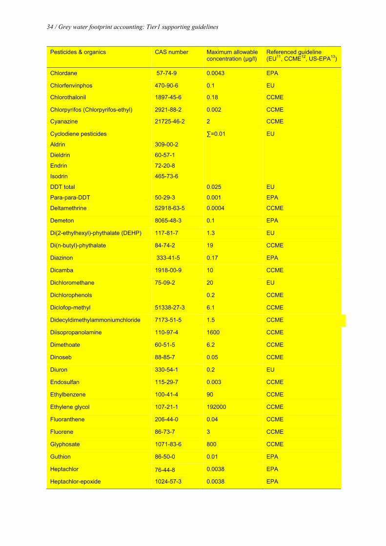
Table 11. Maximum allowable concentrations for pesticides and organics.
Pesticides & organics CAS number Maximum allowable concentration (µg/l)
Referenced guideline (EU11, CCME12, US-EPA13)
1,2 Dichloroethane 107-06-2 10 EU
1,2,3,4 Tetrachlorobenzene 634-66-2 1.8 CCME
1,2,3-Trichlorobenzene 87-61-6 8 CCME
1,2,4- Trichlorobenzene
120-82-1 24 CCME
1,2-Dichlorobenzene 95-50-1 0.7 CCME
1,3-Dichlorobenzene 541-73-1 150 CCME
1,4-Dichlorobenzene 106-46-7 26 CCME
3-lodo-2-prpynyl butylcarbamate 55406-53-6 1.9 CCME
Acenaphthene 83-32-9 5.8 CCME
Acridine 260-94-6 4.4 CCME
Acrolein 107-02-8 3 EPA
Alachlor 15972-60-8 0.3 EU
Aldicarb 116-06-3 1 CCME
Aniline 62-53-3 2.2 CCME
Anthracene 120-12-7 0.012 CCME
Atrazine 1912-24-9 0.6 EU
Benzene 71-43-2 10 EU
Benzo(a)anthracene 56-55-3 0.018 CCME
Benzo(a)pyrene 50-32-8 0.015 CCME
Bromacil 314-40-9 5 CCME
Bromoxynil 1689-84-5 5 CCME
C10-13 Chloroalkanes 85535-84-8 0.4 EU
Captan 133-06-2 1.3 CCME
Carbaryl 63-25-2 0.2 CCME
Carbofuran 1563-66-2 1.8 CCME
Carbon-tetrachloride 56-23-5 12 EU
11 EU (2013): a long-term standard, expressed as an annual average concentration (AA-EQS) and normally based on chronic
toxicity data. 12 CCME (2013): long-term exposure guidelines are meant to protect against all negative effects during indefinite exposures.
They are determined generally based on chronic toxicity data. 13 US-EPA (2013): The Criterion Continuous Concentration (CCC) is an estimate of the highest concentration of a material
in surface water to which an aquatic community can be exposed indefinitely without resulting in an unacceptable effect. US-
EPA derives chronic criteria from longer term (often greater than 28-day) tests that measure survival, growth, or
reproduction.
34 / Grey water footprint accounting: Tier1 supporting guidelines
Pesticides & organics CAS number Maximum allowable concentration (µg/l)
Referenced guideline (EU11, CCME12, US-EPA13)
Chlordane 57-74-9 0.0043 EPA
Chlorfenvinphos 470-90-6 0.1 EU
Chlorothalonil 1897-45-6 0.18 CCME
Chlorpyrifos (Chlorpyrifos-ethyl) 2921-88-2 0.002 CCME
Cyanazine 21725-46-2 2 CCME
Cyclodiene pesticides
Aldrin
Dieldrin
Endrin
Isodrin
309-00-2
60-57-1
72-20-8
465-73-6
∑=0.01 EU
DDT total
Para-para-DDT
50-29-3
0.025
0.001
EU
EPA
Deltamethrine 52918-63-5 0.0004 CCME
Demeton 8065-48-3 0.1 EPA
Di(2-ethylhexyl)-phythalate (DEHP) 117-81-7 1.3 EU
Di(n-butyl)-phythalate 84-74-2 19 CCME
Diazinon 333-41-5 0.17 EPA
Dicamba 1918-00-9 10 CCME
Dichloromethane 75-09-2 20 EU
Dichlorophenols 0.2 CCME
Diclofop-methyl 51338-27-3 6.1 CCME
Didecyldimethylammoniumchloride 7173-51-5 1.5 CCME
Diisopropanolamine 110-97-4 1600 CCME
Dimethoate 60-51-5 6.2 CCME
Dinoseb 88-85-7 0.05 CCME
Diuron 330-54-1 0.2 EU
Endosulfan 115-29-7 0.003 CCME
Ethylbenzene 100-41-4 90 CCME
Ethylene glycol 107-21-1 192000 CCME
Fluoranthene 206-44-0 0.04 CCME
Fluorene 86-73-7 3 CCME
Glyphosate 1071-83-6 800 CCME
Guthion 86-50-0 0.01 EPA
Heptachlor 76-44-8 0.0038 EPA
Heptachlor-epoxide 1024-57-3 0.0038 EPA
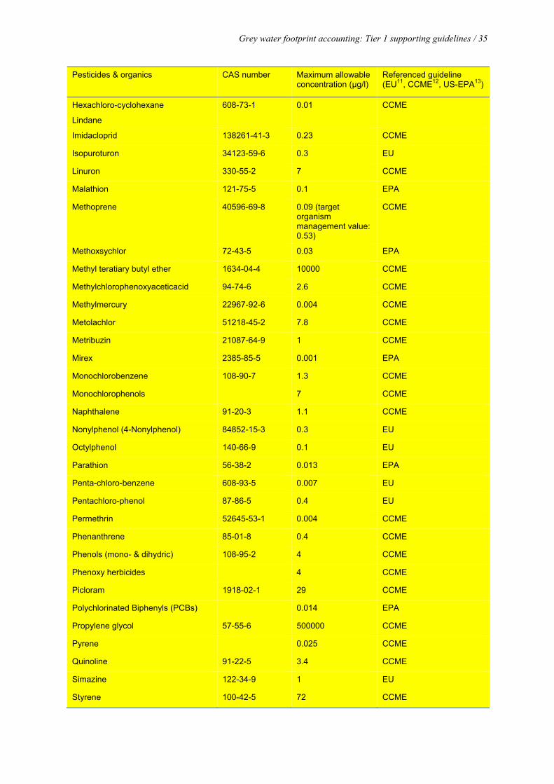
Grey water footprint accounting: Tier 1 supporting guidelines / 35
Pesticides & organics CAS number Maximum allowable concentration (µg/l)
Referenced guideline (EU11, CCME12, US-EPA13)
Hexachloro-cyclohexane
Lindane
608-73-1 0.01 CCME
Imidacloprid 138261-41-3 0.23 CCME
Isopuroturon 34123-59-6 0.3 EU
Linuron 330-55-2 7 CCME
Malathion 121-75-5 0.1 EPA
Methoprene 40596-69-8 0.09 (target organism management value: 0.53)
CCME
Methoxsychlor 72-43-5 0.03 EPA
Methyl teratiary butyl ether 1634-04-4 10000 CCME
Methylchlorophenoxyaceticacid 94-74-6 2.6 CCME
Methylmercury 22967-92-6 0.004 CCME
Metolachlor 51218-45-2 7.8 CCME
Metribuzin 21087-64-9 1 CCME
Mirex 2385-85-5 0.001 EPA
Monochlorobenzene 108-90-7 1.3 CCME
Monochlorophenols 7 CCME
Naphthalene 91-20-3 1.1 CCME
Nonylphenol (4-Nonylphenol) 84852-15-3 0.3 EU
Octylphenol 140-66-9 0.1 EU
Parathion 56-38-2 0.013 EPA
Penta-chloro-benzene 608-93-5 0.007 EU
Pentachloro-phenol 87-86-5 0.4 EU
Permethrin 52645-53-1 0.004 CCME
Phenanthrene 85-01-8 0.4 CCME
Phenols (mono- & dihydric) 108-95-2 4 CCME
Phenoxy herbicides 4 CCME
Picloram 1918-02-1 29 CCME
Polychlorinated Biphenyls (PCBs) 0.014 EPA
Propylene glycol 57-55-6 500000 CCME
Pyrene 0.025 CCME
Quinoline 91-22-5 3.4 CCME
Simazine 122-34-9 1 EU
Styrene 100-42-5 72 CCME
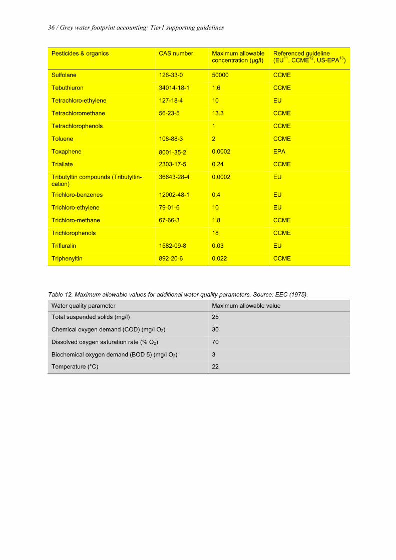
36 / Grey water footprint accounting: Tier1 supporting guidelines
Pesticides & organics CAS number Maximum allowable concentration (µg/l)
Referenced guideline (EU11, CCME12, US-EPA13)
Sulfolane 126-33-0 50000 CCME
Tebuthiuron 34014-18-1 1.6 CCME
Tetrachloro-ethylene 127-18-4 10 EU
Tetrachloromethane 56-23-5 13.3 CCME
Tetrachlorophenols 1 CCME
Toluene 108-88-3 2 CCME
Toxaphene 8001-35-2 0.0002 EPA
Triallate 2303-17-5 0.24 CCME
Tributyltin compounds (Tributyltin-cation)
36643-28-4 0.0002 EU
Trichloro-benzenes 12002-48-1 0.4 EU
Trichloro-ethylene 79-01-6 10 EU
Trichloro-methane 67-66-3 1.8 CCME
Trichlorophenols 18 CCME
Trifluralin 1582-09-8 0.03 EU
Triphenyltin 892-20-6 0.022 CCME
Table 12. Maximum allowable values for additional water quality parameters. Source: EEC (1975).
Water quality parameter Maximum allowable value
Total suspended solids (mg/l) 25
Chemical oxygen demand (COD) (mg/l O2) 30
Dissolved oxygen saturation rate (% O2) 70
Biochemical oxygen demand (BOD 5) (mg/l O2) 3
Temperature (°C) 22
6. What natural background concentration to use
The general definition of natural background level is the concentration that is present owing to natural and
geological processes only, i.e. the background level with no anthropogenic contribution (‘preindustrial’ levels)
(EC, 2011). Natural background concentrations within an environmental compartment may vary by several
orders of magnitude between geologically disparate areas, and are determined by various factors, like site-
specific bedrock composition and the effects of climate on the degree of weathering. Due to natural dynamic
processes like weathering, the addition of organic material (leaves) in autumn and uptake by plants during
spring and summer, natural background concentrations may show annual cycles (Quevauviller et al., 2008). This
variation of water quality over time and space makes it impossible to establish a ‘global’ natural background
level for individual chemical substances, which also would not be very meaningful because of the great
variation (EC, 2011). Therefore we strongly recommend using local data on natural background concentrations.
In more or less pristine rivers, one can assume that natural concentrations are equal to the actual concentrations
and thus rely on long-term daily or monthly averages as measured in a nearby measuring station. For disturbed
rivers, one will have to rely on historical records or model studies (Hoekstra et al., 2011).
EC (2011), a technical guidance document for deriving environmental quality standards, mentions that the
preferred procedure for determining the ‘natural’ background concentrations in freshwater, will usually be to
determine the concentrations in springs or in water bodies in ‘pristine’ areas in the given region, e.g. headwaters.
Another possibility is to measure concentrations in deep groundwater. In some cases, however, the
concentration may be higher in the groundwater than in the surface water, for instance because of the
groundwater’s contact with deep lying mineral rocks or soils and subsequent dilution by rain. Yet another
possibility is to use models to simulate soil processes and erosion, in combination with geochemical database
(like for instance GTK, 2013).
The Canadian water quality guidelines have used the background concentration approach to establish their
objectives (CCME, 2003). The natural background concentrations of a contaminant are estimated and used to
define acceptable water quality conditions at a site under consideration. Three general approaches have been
used to define background concentrations of water quality variables, which involve:
Utilization of historically-collected water quality data for the site (i.e., prior to the commencement of
activities that could have substantially altered water quality conditions);
Monitoring contemporary water quality conditions at one or more stations located upstream of contaminant
sources; and
Monitoring contemporary water quality conditions at one or more reference areas, which are generally
located nearby the site under consideration but have not been adversely affected by human activities.
If local data are not available and time and budget do not allow determining the natural background
concentrations, we suggest using the values in the following tables, which were derived from the
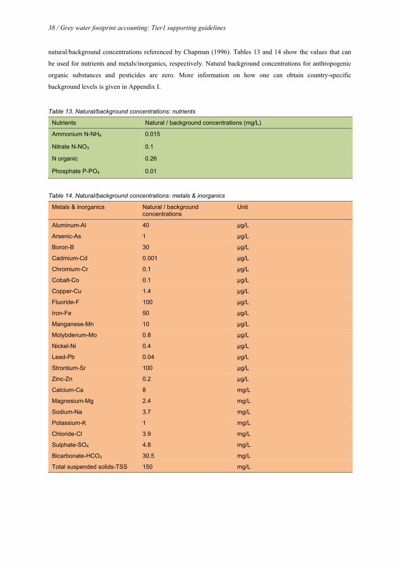
38 / Grey water footprint accounting: Tier1 supporting guidelines
natural/background concentrations referenced by Chapman (1996). Tables 13 and 14 show the values that can
be used for nutrients and metals/inorganics, respectively. Natural background concentrations for anthropogenic
organic substances and pesticides are zero. More information on how one can obtain country-specific
background levels is given in Appendix I.
Table 13. Natural/background concentrations: nutrients
Nutrients Natural / background concentrations (mg/L)
Ammonium N-NH4 0.015
Nitrate N-NO3 0.1
N organic 0.26
Phosphate P-PO4 0.01
Table 14. Natural/background concentrations: metals & inorganics
Metals & inorganics Natural / background concentrations
Unit
Aluminum-Al 40 µg/L
Arsenic-As 1 µg/L
Boron-B 30 µg/L
Cadmium-Cd 0.001 µg/L
Chromium-Cr 0.1 µg/L
Cobalt-Co 0.1 µg/L
Copper-Cu 1.4 µg/L
Fluoride-F 100 µg/L
Iron-Fe 50 µg/L
Manganese-Mn 10 µg/L
Molybdenum-Mo 0.8 µg/L
Nickel-Ni 0.4 µg/L
Lead-Pb 0.04 µg/L
Strontium-Sr 100 µg/L
Zinc-Zn 0.2 µg/L
Calcium-Ca 8 mg/L
Magnesium-Mg 2.4 mg/L
Sodium-Na 3.7 mg/L
Potassium-K 1 mg/L
Chloride-Cl 3.9 mg/L
Sulphate-SO4 4.8 mg/L
Bicarbonate-HCO3 30.5 mg/L
Total suspended solids-TSS 150 mg/L
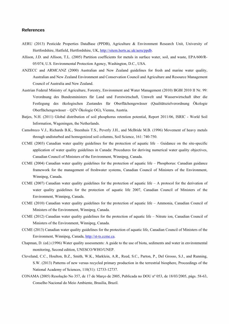
References
AERU (2013) Pesticide Properties DataBase (PPDB), Agriculture & Environment Research Unit, University of
Hertfordshire, Hatfield, Hertfordshire, UK, http://sitem.herts.ac.uk/aeru/ppdb.
Allison, J.D. and Allison, T.L. (2005) Partition coefficients for metals in surface water, soil, and waste, EPA/600/R-
05/074, U.S. Environmental Protection Agency, Washington, D.C., USA.
ANZECC and ARMCANZ (2000) Australian and New Zealand guidelines for fresh and marine water quality,
Australian and New Zealand Environment and Conservation Council and Agriculture and Resource Management
Council of Australia and New Zealand.
Austrian Federal Ministry of Agriculture, Forestry, Environment and Water Management (2010) BGBl 2010 II Nr. 99:
Verordnung des Bundesministers für Land und Forstwirtschaft, Umwelt und Wasserwirtschaft über die
Festlegung des ökologischen Zustandes für Oberflächengewässer (Qualitätszielverordnung Ökologie
Oberflächengewässer – QZV Ökologie OG), Vienna, Austria.
Batjes, N.H. (2011) Global distribution of soil phosphorus retention potential, Report 2011/06, ISRIC - World Soil
Information, Wageningen, the Netherlands.
Camobreco V.J., Richards B.K., Steenhuis T.S., Peverly J.H., and McBride M.B. (1996) Movement of heavy metals
through undisturbed and homogenized soil columns, Soil Science, 161: 740-750.
CCME (2003) Canadian water quality guidelines for the protection of aquatic life – Guidance on the site-specific
application of water quality guidelines in Canada: Procedures for deriving numerical water quality objectives,
Canadian Council of Ministers of the Environment, Winnipeg, Canada.
CCME (2004) Canadian water quality guidelines for the protection of aquatic life – Phosphorus: Canadian guidance
framework for the management of freshwater systems, Canadian Council of Ministers of the Environment,
Winnipeg, Canada.
CCME (2007) Canadian water quality guidelines for the protection of aquatic life – A protocol for the derivation of
water quality guidelines for the protection of aquatic life 2007, Canadian Council of Ministers of the
Environment, Winnipeg, Canada.
CCME (2010) Canadian water quality guidelines for the protection of aquatic life – Ammonia, Canadian Council of
Ministers of the Environment, Winnipeg, Canada.
CCME (2012) Canadian water quality guidelines for the protection of aquatic life – Nitrate ion, Canadian Council of
Ministers of the Environment, Winnipeg, Canada.
CCME (2013) Canadian water quality guidelines for the protection of aquatic life, Canadian Council of Ministers of the
Environment, Winnipeg, Canada, http://st-ts.ccme.ca.
Chapman, D. (ed.) (1996) Water quality assessments: A guide to the use of biota, sediments and water in environmental
monitoring, Second edition, UNESCO/WHO/UNEP.
Cleveland, C.C., Houlton, B.Z., Smith, W.K., Marklein, A.R., Reed, S.C., Parton, P., Del Grosso, S.J., and Running,
S.W. (2013) Patterns of new versus recycled primary production in the terrestrial biosphere, Proceedings of the
National Academy of Sciences, 110(31): 12733-12737.
CONAMA (2005) Resolução No 357, de 17 de Março de 2005, Publicada no DOU nº 053, de 18/03/2005, págs. 58-63,
Conselho Nacional do Meio Ambiente, Brasilia, Brazil.
40 / Grey water footprint accounting: Tier1 supporting guidelines
DWAF (1996) South African water quality guidelines, Volume 7 Aquatic ecosystems, Second edition, Department of
Water Affairs and Forestry, Pretoria, South Africa.
EEA (2005) Gross nutrient balance (CSI 025), European Environment Agency, Copenhagen, Denmark,
www.eea.europa.eu/data-and-maps/indicators/gross-nutrient-balance-1.
EEC (1975) Quality required of surface water intended for the abstraction of drinking water in the Member States,
Council Directive 75/440/EEC, European Economic Community, Brussels, Belgium.
EC (2008) Environmental quality standards in the field of water policy, Directive 2008/105/EC of the European
Parliament and of the Council, European Commission, Brussels, Belgium.
EC (2011) Common implementation strategy for the Water Framework Directive (2000/60/EC), Guidance Document
No. 27: Technical guidance for deriving environmental quality standards, Technical Report 2011-055, European
Commission, Brussels, Belgium.
EU (2013) Directive 2013/39/EU of the European Parliament and of the Council amending Directives 2000/60/EC and
2008/105/EC as regards priority substances in the field of water policy, European Union, Brussels, Belgium.
FAO (2013a) GeoNetwork, Food and Agriculture Organization, Rome, Italy, www.fao.org/geonetwork.
FAO (2013b) FAOSTAT, Food and Agriculture Organization, Rome, Italy, http://faostat3.fao.org/faostat-
gateway/go/to/home/E.
Feick, S., Siebert, S. and Döll, P. (2005) A digital global map of artificially drained agricultural areas, Frankfurt
Hydrology Paper 04, Institute of Physical Geography, Frankfurt University, Frankfurt am Main, Germany.
Garrabrants, A.C. Kosson, D.S., Van der Sloot, H.A., Sanchez, F. and Hjelmar, O. (2010) Background information for
the leaching environmental assessment framework (LEAF) test methods, EPA/600/R-10/170, U.S.
Environmental Protection Agency, Washington, D.C., USA.
GTK (2013) FOREGS Geochemical Atlas of Europe, Geological Survey of Finland, http://weppi.gtk.fi/publ/foregsatlas.
Hem, J.D. (1985) Study and interpretation of the chemical characteristics of natural water, Third edition, Water Supply
Paper 2254, U.S Geological Survey, Alexandria, VA, USA.
Hoekstra, A.Y., Chapagain, A.K., Aldaya, M.M. and Mekonnen, M.M. (2011) The water footprint assessment manual:
Setting the global standard, Earthscan, London, UK.
IIASA (2013) Harmonized world soil database, International Institute for Applied Systems Analysis, Laxenburg,
Austria, http://www.iiasa.ac.at/Research/LUC/External-World-soil-database/HTML.
IPCC (2006) 2006 IPCC guidelines for national greenhouse gas inventories, Intergovernmental Panel on Climate
Change, www.ipcc-nggip.iges.or.jp.
JRC (2013) European Soil Portal, Institute for Environment and Sustainability, Joint Research Centre, European
Commission, Ispra, Italy, http://eusoils.jrc.ec.europa.eu.
Koirala, S. (2013) Soil texture maps, Hirabayashi lab, University of Tokyo, Japan, http://hydro.iis.u-
tokyo.ac.jp/~sujan/home.html.
LAWA-AO (2007) Rahmenkonzeption Monitoring, Teil B Bewertungsgrundlagen und Methodenbeschreibungen –
Arbeitspapier II Hintergrund- und Orientierungswerte fu�r physikalisch-chemische Komponenten,
Bund/Länder-Arbeitsgemeinschaft Wasser, Magdeburg, Germany.
MacDonald, G.K., Bennett, E.M., Potter, P.A. and Ramankutty, N. (2011) Agronomic phosphorus imbalances across
the world’s croplands, Proceedings of the National Academy of Sciences, 108(7): 3086-3091.
Grey water footprint accounting: Tier 1 supporting guidelines / 41
McLean, J.E. and Bledsoe, B.E. (1992) Ground water issue: Behavior of metals in soils, EPA/540/S-92/018, U.S.
Environmental Protection Agency, Washington, D.C., USA.
MEP (1994) Quality standard for ground water, GB/T 14848-93, Ministry of Environmental Protection, The People’s
Republic of China, Beijing, China.
MEP (2002) Environmental quality standard for surface water, GB 3838-2002, Ministry of Environmental Protection,
The People’s Republic of China, Beijing, China.
Ministry of the Environment (2010) Environmental quality standards for water pollution, Ministry of the Environment,
Government of Japan, Tokyo, Japan, www.env.go.jp/en/water/wq/wp.pdf.
National Research Council (1993) Soil and water quality: an agenda for agriculture, Committee on Long-Range Soil
and Water Conservation, Board on Agriculture, National Academy Press, Washington, D.C., USA.
Osté, L.A., Klein, J. and Zwolsman, G.J. (2011) Inventory and evaluation of methods to derive natural background
concentrations of trace metals in surface water, and application of two methods in a case study, Deltares report
1206111.005, Utrecht, the Netherlands.
Quevauviller, P.P., Borchers, U., Thompson, C. and Simonart, T. (eds.) (2008) The water framework directive:
Ecological and chemical status monitoring, John Wiley & Sons, Chichester, UK.
Roy, R.N., Finck, A., Blair G.J. and Tandon H.L.S. (2006) Chapter 8 Nutrient management guidelines for some major
field crops, In: Plant nutrition for food security: A guide for integrated nutrient management, FAO Fertilizer and
Plant Nutrition Bulletin 16, Food and Agriculture Organization, Rome, Italy.
SAGE (2013), The atlas of the biosphere, Center for Sustainability and the Global Environment (SAGE), Nelson
Institute for Environmental Studies, University of Wisconsin, Madison, USA,
www.sage.wisc.edu/atlas/maps.php.
Scharlemann, J.P.W., Hiederer, R., Kapos, V. and Ravilious, C. (2011) Updated global carbon map, World
Conservation Monitoring Centre, United Nations Environment Programme, Nairobi, Kenya.
Simmelsgaard, S.E. (1998) The effect of crop, N-level, soil type and drainage on nitrate leaching from Danish soil, Soil
Use and Management, 14(1): 30-36.
Thompson, T., Fawell, J., Kunikane, S., Jackson, D., Appleyard, S., Callan, P., Bartram, J. and Kingston, P. (2007)
Chemical safety of drinking-water: Assessing priorities for risk management, World Health Organization,
Geneva, Switzerland.
UKTAG (2008) UK environmental standards and conditions – Phase 1 & Phase 2, UK Technical Advisory Group on
the Water Framework Directive, UK.
UKTAG (2013) Updated recommendations on environmental standards: River basin management, Final report, UK
Technical Advisory Group on the Water Framework Directive, UK.
UNEP (2009) GEMStat: Global Environment Monitoring System (GEMS) Water Programme, United Nations
Environment Programme, Nairobi, Kenya, www.gemstat.org.
USDA (1997) Water quality and agriculture: Status, conditions, and trends, Working Paper #16, Natural Resources
Conservation Service, United States Department of Agriculture, Washington, D.C., USA.
USDA (2013a) Soils, Natural Resources Conservation Service, United States Department of Agriculture, Washington,
D.C., USA, www.nrcs.usda.gov/wps/portal/nrcs/site/soils.
USDA (2013b) Nutrient content of crops, Natural Resources Conservation Service, United States Department of
Agriculture, Washington, D.C., USA, http://plants.usda.gov/npk/main.
42 / Grey water footprint accounting: Tier1 supporting guidelines
US-EPA (1996a) Soil screening guidance: Users guide, Second edition, EPA/540/R-96/018, United States
Environmental Protection Agency, Washington, D.C., USA.
US-EPA (1996b) Soil screening guidance: Technical background document, Second edition, EPA/540/R-95/128,
United States Environmental Protection Agency, Washington, D.C., USA.
US-EPA (1999) Understanding variation in partition coefficient, Kd, values, Volume II: Review of geochemistry and
available Kd values for cadmium, cesium, chromium, lead, plutonium, radon, strontium, thorium, tritium (3H),
and uranium, EPA 402-R-99-004B, U.S. Environmental Protection Agency, Washington, D.C., USA.
US-EPA (2012) Water quality standards handbook: Second edition, EPA-823-B-12-002, Environmental Protection
Agency, Washington, D.C., USA.
US-EPA (2013) National recommended water quality criteria – aquatic life criteria, Environmental Protection Agency,
Washington, D.C., USA, http://water.epa.gov/scitech/swguidance/standards/criteria/current/index.cfm.
Wauchope, R.D., Buttler, T.M., Hornsby, A.G., Augustijn-Beckers, P.W.M. and Burt, J.P. (1992) The SCS/ARS/CES
pesticide properties database for environmental decision- making, Reviews of Environmental Contamination and
Toxicology, 123: 1-156.
Wischmeier, W.H. and Smith, D.D. (1978) Predicting rainfall erosion losses: A guide to conservation planning,
Agriculture Handbook No. 537, United States Department of Agriculture, Washington, D.C., USA.
Yang X., Post W.M., Thornton P.E., and Jain A. (2013) The distribution of soil phosphorus for global biogeochemical
modelling, Biogeosciences, 10(4): 2525–2537.
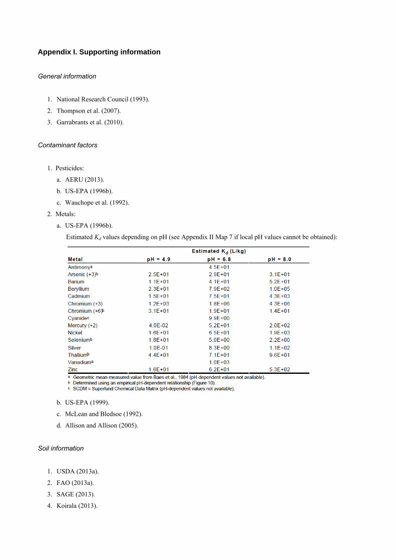
Appendix I. Supporting information
General information
1. National Research Council (1993).
2. Thompson et al. (2007).
3. Garrabrants et al. (2010).
Contaminant factors
1. Pesticides:
a. AERU (2013).
b. US-EPA (1996b).
c. Wauchope et al. (1992).
2. Metals:
a. US-EPA (1996b).
Estimated Kd values depending on pH (see Appendix II Map 7 if local pH values cannot be obtained):
b. US-EPA (1999).
c. McLean and Bledsoe (1992).
d. Allison and Allison (2005).
Soil information
1. USDA (2013a).
2. FAO (2013a).
3. SAGE (2013).
4. Koirala (2013).
44 / Grey water footprint accounting: Tier1 supporting guidelines
5. JRC (2013).
6. IIASA (2013).
7. MacDonald et al. (2011).
8. Batjes (2011).
9. Cleveland et al. (2013).
10. Yang et al. (2013).
11. Scharlemann et al. (2011).
Nutrient surplus
1. FAO (2013b).
2. Roy et al. (2006).
3. USDA (2013b)
4. EEA (2005).
Maximum allowable concentrations
1. Australia and New Zealand: ANZECC and ARMCANZ (2000).
2. Austria: Austrian Federal Ministry of Agriculture, Forestry, Environment and Water Management (2010).
3. Brazil: CONAMA (2005).
4. Canada: CCME (2013).
5. China: MEP (1994, 2002).
6. European Union: EC (2008).
7. Germany LAWA-AO (2007).
8. Japan: Ministry of the Environment (2010).
9. South Africa: DWAF (1996).
10. United Kingdom: UKTAG (2008, 2013).
11. United States: US-EPA (2012, 2013).
Natural background concentrations
1. As a reference, a global database on actual (not natural) concentrations is available through UNEP (2009).
2. Using the geochemical atlas of GTK (2013), natural background concentrations can be derived, using the
guidelines of EC (2011).
3. For several parts of the world, for specific substances, good studies are available, for example: United States:
Hem (1985); Austria: Austrian Federal Ministry of Agriculture, Forestry, Environment and Water Management
(2010); Germany: LAWA-AO (2007); The Netherlands: Osté et al. (2011).
Appendix II. Leaching-runoff influencing factor maps
Map 1. Global N deposition. Source: Cleveland et al. (2013).
Map 2. Global average soil texture. Source: Koirala (2013).
Map 3. Soil drainage class. Source: FAO (2013a).
Map 4. Global map of artificially drained agricultural areas. Source: Feick et al. (2005).
Map 5. Global average annual precipitation. Source: FAO (2013a).
Map 6. Global distribution of total phosphorous content (g P/m2) in soil. Source: Yang et al. (2013).
Map 7. pH topsoil. Source: FAO (2013a).
Map 8. Organic carbon. Source: Scharlemann et al. (2011).
Map 9. Water erosion vulnerability. Source: USDA (2013a).
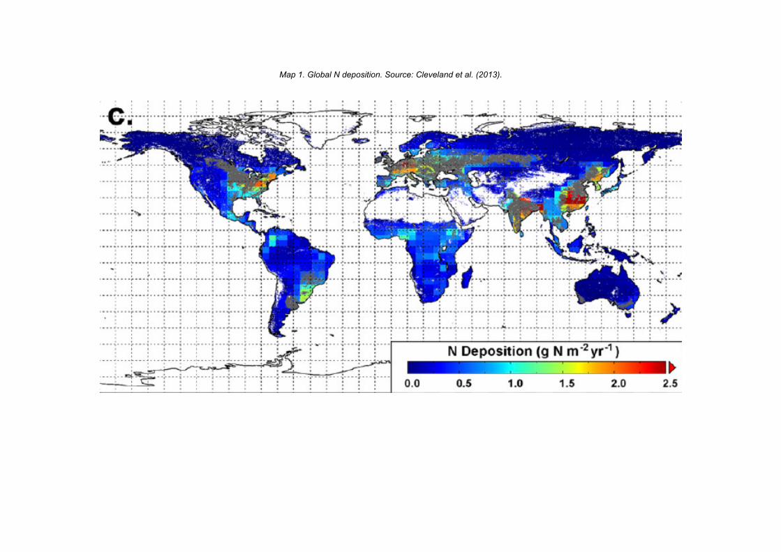
Map 1. Global N deposition. Source: Cleveland et al. (2013).
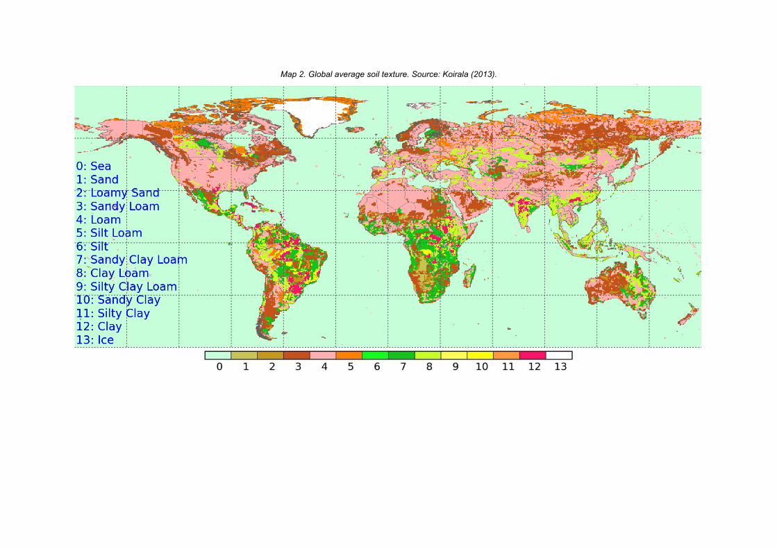
Map 2. Global average soil texture. Source: Koirala (2013).
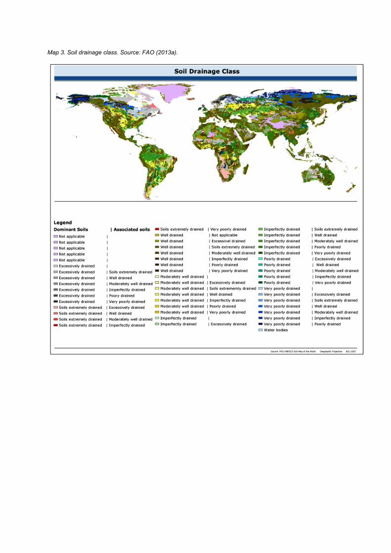
Map 3. Soil drainage class. Source: FAO (2013a).
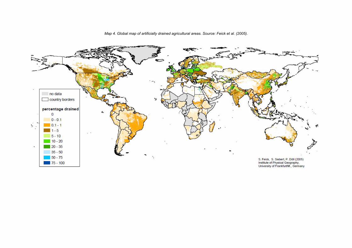
Map 4. Global map of artificially drained agricultural areas. Source: Feick et al. (2005).
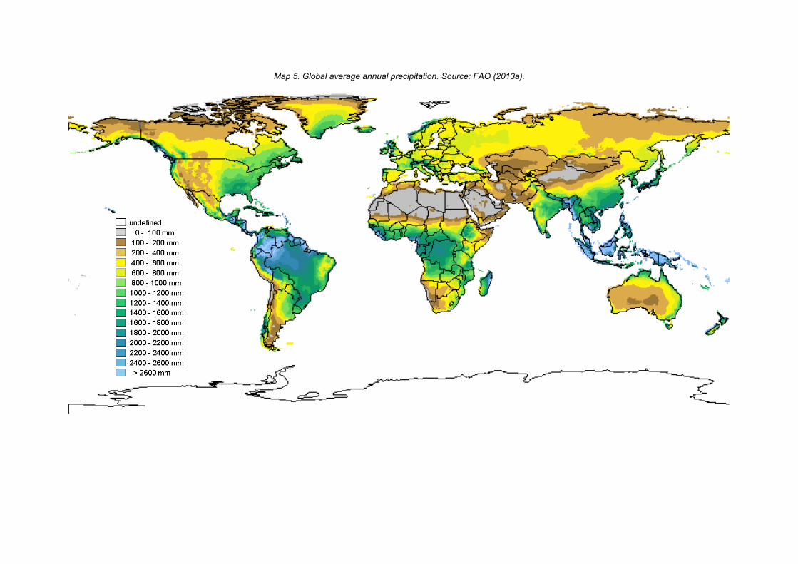
Map 5. Global average annual precipitation. Source: FAO (2013a).
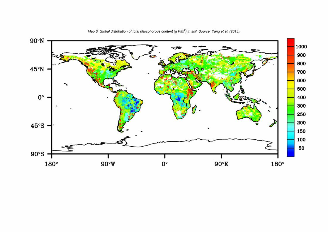
Map 6. Global distribution of total phosphorous content (g P/m2) in soil. Source: Yang et al. (2013).
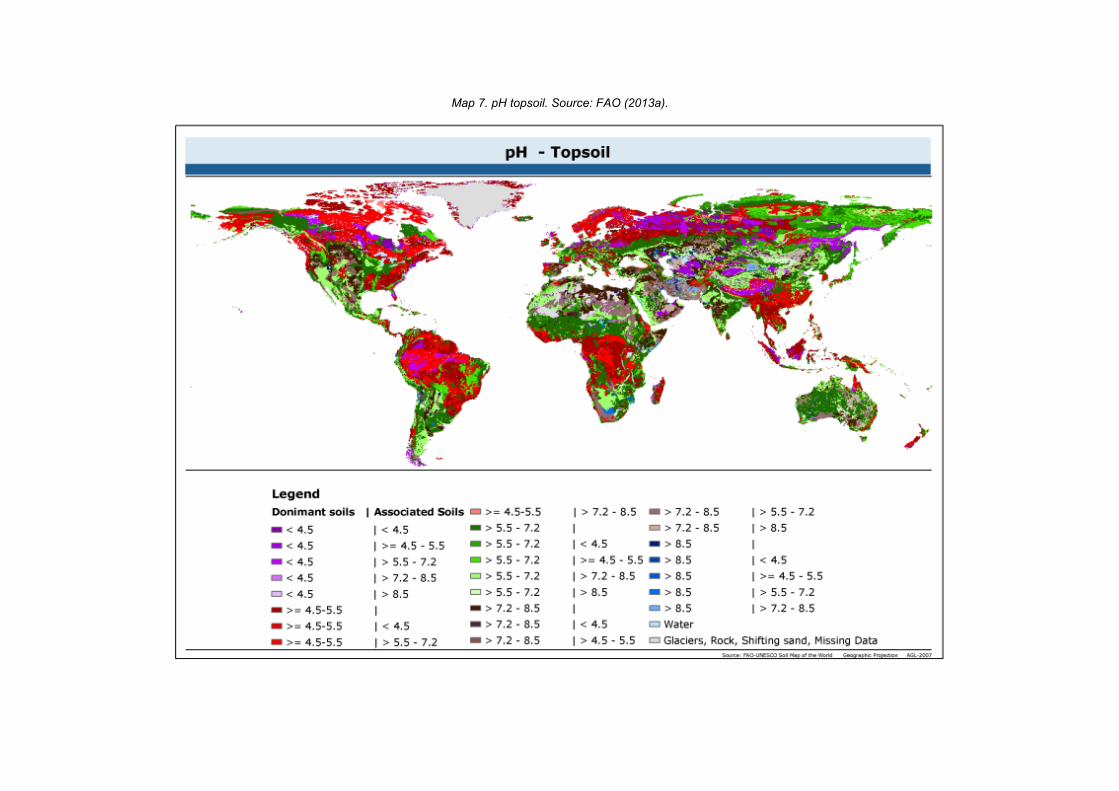
Map 7. pH topsoil. Source: FAO (2013a).
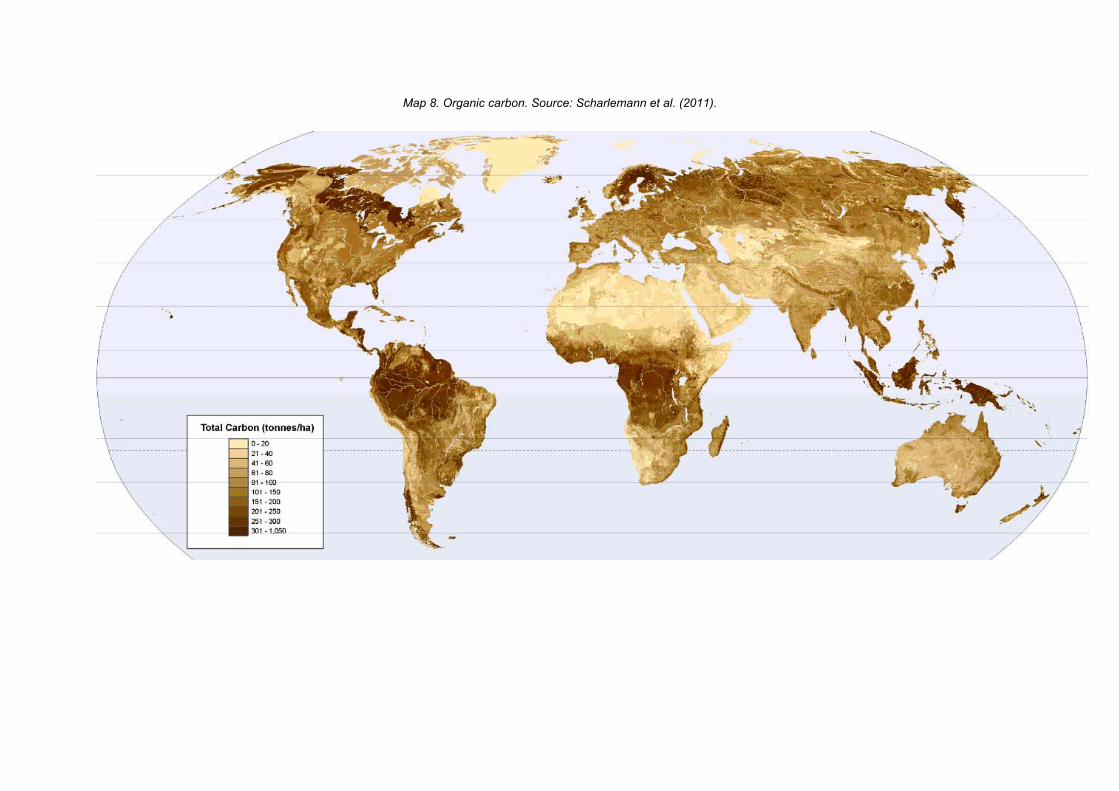
Map 8. Organic carbon. Source: Scharlemann et al. (2011).
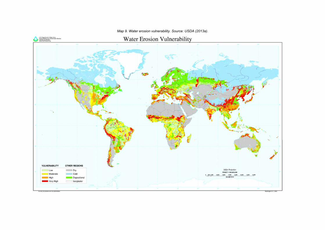
Map 9. Water erosion vulnerability. Source: USDA (2013a).
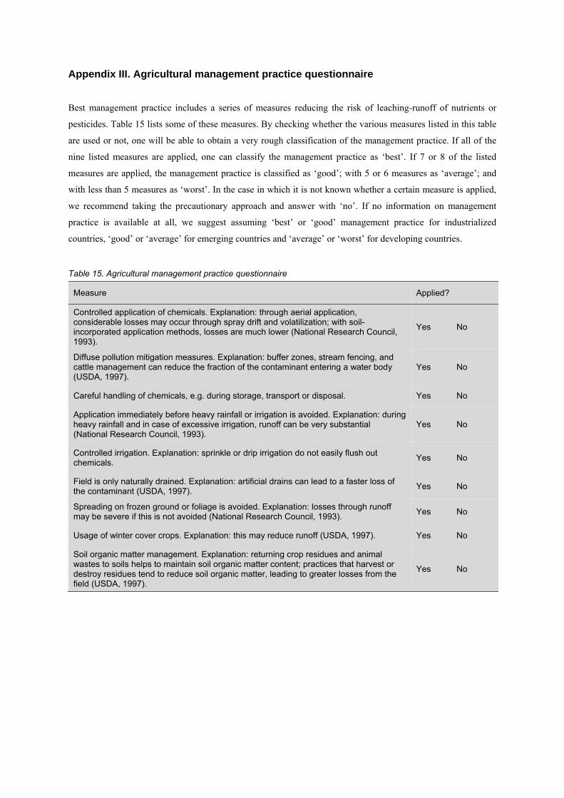
Appendix III. Agricultural management practice questionnaire
Best management practice includes a series of measures reducing the risk of leaching-runoff of nutrients or
pesticides. Table 15 lists some of these measures. By checking whether the various measures listed in this table
are used or not, one will be able to obtain a very rough classification of the management practice. If all of the
nine listed measures are applied, one can classify the management practice as ‘best’. If 7 or 8 of the listed
measures are applied, the management practice is classified as ‘good’; with 5 or 6 measures as ‘average’; and
with less than 5 measures as ‘worst’. In the case in which it is not known whether a certain measure is applied,
we recommend taking the precautionary approach and answer with ‘no’. If no information on management
practice is available at all, we suggest assuming ‘best’ or ‘good’ management practice for industrialized
countries, ‘good’ or ‘average’ for emerging countries and ‘average’ or ‘worst’ for developing countries.
Table 15. Agricultural management practice questionnaire
Measure Applied?
Controlled application of chemicals. Explanation: through aerial application, considerable losses may occur through spray drift and volatilization; with soil-incorporated application methods, losses are much lower (National Research Council, 1993).
Yes No
Diffuse pollution mitigation measures. Explanation: buffer zones, stream fencing, and cattle management can reduce the fraction of the contaminant entering a water body (USDA, 1997).
Yes No
Careful handling of chemicals, e.g. during storage, transport or disposal. Yes No
Application immediately before heavy rainfall or irrigation is avoided. Explanation: during heavy rainfall and in case of excessive irrigation, runoff can be very substantial (National Research Council, 1993).
Yes No
Controlled irrigation. Explanation: sprinkle or drip irrigation do not easily flush out chemicals.
Yes No
Field is only naturally drained. Explanation: artificial drains can lead to a faster loss of the contaminant (USDA, 1997).
Yes No
Spreading on frozen ground or foliage is avoided. Explanation: losses through runoff may be severe if this is not avoided (National Research Council, 1993).
Yes No
Usage of winter cover crops. Explanation: this may reduce runoff (USDA, 1997). Yes No
Soil organic matter management. Explanation: returning crop residues and animal wastes to soils helps to maintain soil organic matter content; practices that harvest or destroy residues tend to reduce soil organic matter, leading to greater losses from the field (USDA, 1997).
Yes No

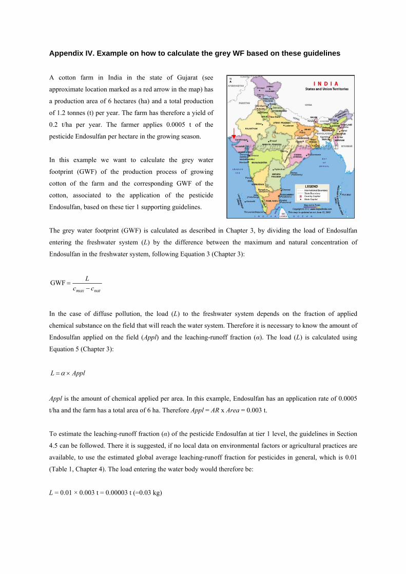
Appendix IV. Example on how to calculate the grey WF based on these guidelines
A cotton farm in India in the state of Gujarat (see
approximate location marked as a red arrow in the map) has
a production area of 6 hectares (ha) and a total production
of 1.2 tonnes (t) per year. The farm has therefore a yield of
0.2 t/ha per year. The farmer applies 0.0005 t of the
pesticide Endosulfan per hectare in the growing season.
In this example we want to calculate the grey water
footprint (GWF) of the production process of growing
cotton of the farm and the corresponding GWF of the
cotton, associated to the application of the pesticide
Endosulfan, based on these tier 1 supporting guidelines.
The grey water footprint (GWF) is calculated as described in Chapter 3, by dividing the load of Endosulfan
entering the freshwater system (L) by the difference between the maximum and natural concentration of
Endosulfan in the freshwater system, following Equation 3 (Chapter 3):
natmax cc
L
GWF
In the case of diffuse pollution, the load (L) to the freshwater system depends on the fraction of applied
chemical substance on the field that will reach the water system. Therefore it is necessary to know the amount of
Endosulfan applied on the field (Appl) and the leaching-runoff fraction (α). The load (L) is calculated using
Equation 5 (Chapter 3):
ApplL
Appl is the amount of chemical applied per area. In this example, Endosulfan has an application rate of 0.0005
t/ha and the farm has a total area of 6 ha. Therefore Appl = AR x Area = 0.003 t.
To estimate the leaching-runoff fraction (α) of the pesticide Endosulfan at tier 1 level, the guidelines in Section
4.5 can be followed. There it is suggested, if no local data on environmental factors or agricultural practices are
available, to use the estimated global average leaching-runoff fraction for pesticides in general, which is 0.01
(Table 1, Chapter 4). The load entering the water body would therefore be:
L = 0.01 × 0.003 t = 0.00003 t (=0.03 kg)
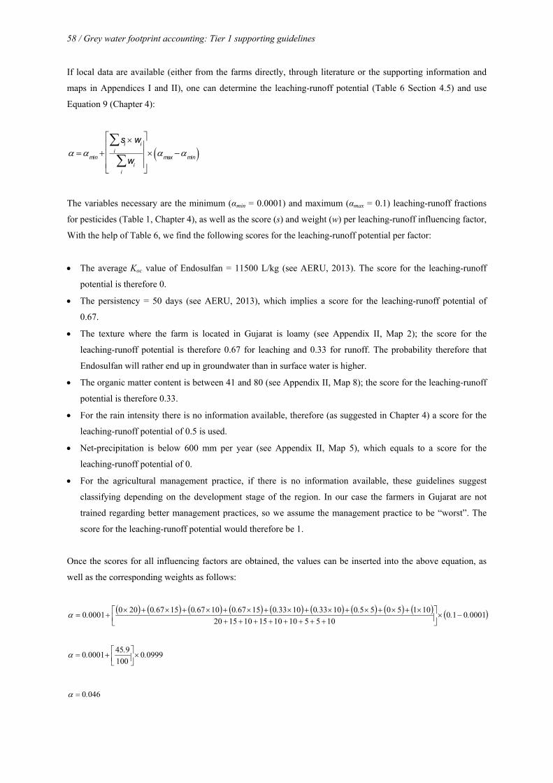
58 / Grey water footprint accounting: Tier 1 supporting guidelines
If local data are available (either from the farms directly, through literature or the supporting information and
maps in Appendices I and II), one can determine the leaching-runoff potential (Table 6 Section 4.5) and use
Equation 9 (Chapter 4):
min
siw
ii
w
ii
max
min
The variables necessary are the minimum (αmin = 0.0001) and maximum (αmax = 0.1) leaching-runoff fractions
for pesticides (Table 1, Chapter 4), as well as the score (s) and weight (w) per leaching-runoff influencing factor,
With the help of Table 6, we find the following scores for the leaching-runoff potential per factor:
The average Koc value of Endosulfan = 11500 L/kg (see AERU, 2013). The score for the leaching-runoff
potential is therefore 0.
The persistency = 50 days (see AERU, 2013), which implies a score for the leaching-runoff potential of
0.67.
The texture where the farm is located in Gujarat is loamy (see Appendix II, Map 2); the score for the
leaching-runoff potential is therefore 0.67 for leaching and 0.33 for runoff. The probability therefore that
Endosulfan will rather end up in groundwater than in surface water is higher.
The organic matter content is between 41 and 80 (see Appendix II, Map 8); the score for the leaching-runoff
potential is therefore 0.33.
For the rain intensity there is no information available, therefore (as suggested in Chapter 4) a score for the
leaching-runoff potential of 0.5 is used.
Net-precipitation is below 600 mm per year (see Appendix II, Map 5), which equals to a score for the
leaching-runoff potential of 0.
For the agricultural management practice, if there is no information available, these guidelines suggest
classifying depending on the development stage of the region. In our case the farmers in Gujarat are not
trained regarding better management practices, so we assume the management practice to be “worst”. The
score for the leaching-runoff potential would therefore be 1.
Once the scores for all influencing factors are obtained, the values can be inserted into the above equation, as
well as the corresponding weights as follows:
00010101055101015101520
10150550103301033015670106701567020000010 ..
.......
09990100
94500010 .
..
0460.
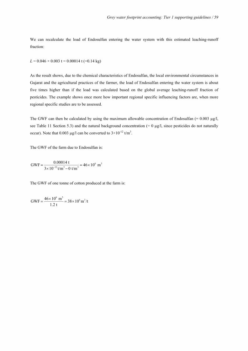
Grey water footprint accounting: Tier 1 supporting guidelines / 59
We can recalculate the load of Endosulfan entering the water system with this estimated leaching-runoff
fraction:
L = 0.046 × 0.003 t = 0.00014 t (=0.14 kg)
As the result shows, due to the chemical characteristics of Endosulfan, the local environmental circumstances in
Gujarat and the agricultural practices of the farmer, the load of Endosulfan entering the water system is about
five times higher than if the load was calculated based on the global average leaching-runoff fraction of
pesticides. The example shows once more how important regional specific influencing factors are, when more
regional specific studies are to be assessed.
The GWF can then be calculated by using the maximum allowable concentration of Endosulfan (= 0.003 µg/l,
see Table 11 Section 5.3) and the natural background concentration (= 0 µg/l, since pesticides do not naturally
occur). Note that 0.003 µg/l can be converted to 3×10-12 t/m3.
The GWF of the farm due to Endosulfan is:
GWF 0.00014 t
31012 t/m3 0 t/m3 46106 m3
The GWF of one tonne of cotton produced at the farm is:
GWF 46106 m3
1.2 t 38106 m3 /t

Value of Water Research Report Series
Editorial board: A.Y. Hoekstra, University of Twente; H.H.G. Savenije, Delft University of Technology; P. van der Zaag, UNESCO-IHE. Reports can be downloaded from: www.waterfootprint.org and www.unesco-ihe.org/value-of-water-research-report-series. 1. Exploring methods to assess the value of water: A case study on the Zambezi basin
A.K. Chapagain February 2000 2. Water value flows: A case study on the Zambezi basin.
A.Y. Hoekstra, H.H.G. Savenije and A.K. Chapagain March 2000 3. The water value-flow concept
I.M. Seyam and A.Y. Hoekstra December 2000 4. The value of irrigation water in Nyanyadzi smallholder irrigation scheme, Zimbabwe G.T. Pazvakawambwa and P. van der Zaag – January 2001 5. The economic valuation of water: Principles and methods J.I. Agudelo – August 2001 6. The economic valuation of water for agriculture: A simple method applied to the eight Zambezi basin countries J.I. Agudelo and A.Y. Hoekstra – August 2001 7. The value of freshwater wetlands in the Zambezi basin I.M. Seyam, A.Y. Hoekstra, G.S. Ngabirano and H.H.G. Savenije – August 2001 8. ‘Demand management’ and ‘Water as an economic good’: Paradigms with pitfalls H.H.G. Savenije and P. van der Zaag – October 2001 9. Why water is not an ordinary economic good H.H.G. Savenije – October 2001 10. Calculation methods to assess the value of upstream water flows and storage as a function of downstream benefits I.M. Seyam, A.Y. Hoekstra and H.H.G. Savenije – October 2001 11. Virtual water trade: A quantification of virtual water flows between nations in relation to international crop trade A.Y. Hoekstra and P.Q. Hung – September 2002 12. Virtual water trade: Proceedings of the international expert meeting on virtual water trade, IHE Delft, the Netherlands, 12-13 December 2002 A.Y. Hoekstra (ed.) – February 2003 13. Virtual water flows between nations in relation to trade in livestock and livestock products A.K. Chapagain and A.Y. Hoekstra – July 2003 14. The water needed to have the Dutch drink coffee A.K. Chapagain and A.Y. Hoekstra – August 2003 15. The water needed to have the Dutch drink tea A.K. Chapagain and A.Y. Hoekstra – August 2003 16. Water footprints of nations, Volume 1: Main Report, Volume 2: Appendices A.K. Chapagain and A.Y. Hoekstra – November 2004 17. Saving water through global trade A.K. Chapagain, A.Y. Hoekstra and H.H.G. Savenije – September 2005 18. The water footprint of cotton consumption A.K. Chapagain, A.Y. Hoekstra, H.H.G. Savenije and R. Gautam – September 2005 19. Water as an economic good: the value of pricing and the failure of markets P. van der Zaag and H.H.G. Savenije – July 2006 20. The global dimension of water governance: Nine reasons for global arrangements in order to cope with local water problems A.Y. Hoekstra – July 2006 21. The water footprints of Morocco and the Netherlands A.Y. Hoekstra and A.K. Chapagain – July 2006 22. Water’s vulnerable value in Africa P. van der Zaag – July 2006 23. Human appropriation of natural capital: Comparing ecological footprint and water footprint analysis A.Y. Hoekstra – July 2007 24. A river basin as a common-pool resource: A case study for the Jaguaribe basin in Brazil P.R. van Oel, M.S. Krol and A.Y. Hoekstra – July 2007 25. Strategic importance of green water in international crop trade M.M. Aldaya, A.Y. Hoekstra and J.A. Allan – March 2008 26. Global water governance: Conceptual design of global institutional arrangements M.P. Verkerk, A.Y. Hoekstra and P.W. Gerbens-Leenes – March 2008 27. Business water footprint accounting: A tool to assess how production of goods and services impact on freshwater resources worldwide P.W. Gerbens-Leenes and A.Y. Hoekstra – March 2008 28. Water neutral: reducing and offsetting the impacts of water footprints A.Y. Hoekstra – March 2008 29. Water footprint of bio-energy and other primary energy carriers P.W. Gerbens-Leenes, A.Y. Hoekstra and Th.H. van der Meer – March 2008 30. Food consumption patterns and their effect on water requirement in China J. Liu and H.H.G. Savenije – March 2008 31. Going against the flow: A critical analysis of virtual water trade in the context of India’s National River Linking Programme S. Verma, D.A. Kampman, P. van der Zaag and A.Y. Hoekstra – March 2008 32. The water footprint of India D.A. Kampman, A.Y. Hoekstra and M.S. Krol – May 2008 33. The external water footprint of the Netherlands: Quantification and impact assessment P.R. van Oel, M.M. Mekonnen and A.Y. Hoekstra – May 2008 34. The water footprint of bio-energy: Global water use for bio-ethanol, bio-diesel, heat and electricity P.W. Gerbens-Leenes, A.Y. Hoekstra and Th.H. van der Meer – August 2008
35. Water footprint analysis for the Guadiana river basin M.M. Aldaya and M.R. Llamas – November 2008 36. The water needed to have Italians eat pasta and pizza M.M. Aldaya and A.Y. Hoekstra – May 2009 37. The water footprint of Indonesian provinces related to the consumption of crop products F. Bulsink, A.Y. Hoekstra and M.J. Booij – May 2009 38. The water footprint of sweeteners and bio-ethanol from sugar cane, sugar beet and maize P.W. Gerbens-Leenes and A.Y. Hoekstra – November 2009 39. A pilot in corporate water footprint accounting and impact assessment: The water footprint of a sugar-containing carbonated beverage A.E. Ercin, M.M. Aldaya and A.Y. Hoekstra – November 2009 40. The blue, green and grey water footprint of rice from both a production and consumption perspective A.K. Chapagain and A.Y. Hoekstra – March 2010 41. Water footprint of cotton, wheat and rice production in Central Asia M.M. Aldaya, G. Muñoz and A.Y. Hoekstra – March 2010 42. A global and high-resolution assessment of the green, blue and grey water footprint of wheat M.M. Mekonnen and A.Y. Hoekstra – April 2010 43. Biofuel scenarios in a water perspective: The global blue and green water footprint of road transport in 2030 A.R. van Lienden, P.W. Gerbens-Leenes, A.Y. Hoekstra and Th.H. van der Meer – April 2010 44. Burning water: The water footprint of biofuel-based transport P.W. Gerbens-Leenes and A.Y. Hoekstra – June 2010 45. Mitigating the water footprint of export cut flowers from the Lake Naivasha Basin, Kenya M.M. Mekonnen and A.Y. Hoekstra – June 2010 46. The green and blue water footprint of paper products: methodological considerations and quantification P.R. van Oel and A.Y. Hoekstra – July 2010 47. The green, blue and grey water footprint of crops and derived crop products M.M. Mekonnen and A.Y. Hoekstra – December 2010 48. The green, blue and grey water footprint of animals and derived animal products M.M. Mekonnen and A.Y. Hoekstra – December 2010 49. The water footprint of soy milk and soy burger and equivalent animal products A.E. Ercin, M.M. Aldaya and A.Y. Hoekstra – February 2011 50. National water footprint accounts: The green, blue and grey water footprint of production and consumption M.M. Mekonnen and A.Y. Hoekstra – May 2011 51. The water footprint of electricity from hydropower M.M. Mekonnen and A.Y. Hoekstra – June 2011 52. The relation between national water management and international trade: a case study from Kenya M.M. Mekonnen and A.Y. Hoekstra – June 2011 53. Global water scarcity: The monthly blue water footprint compared to blue water availability for the world’s major river basins A.Y. Hoekstra and M.M. Mekonnen – September 2011 54. Proceedings of the ESF Strategic Workshop on accounting for water scarcity and pollution in the rules of international trade A.Y. Hoekstra, M.M. Aldaya and B. Avril (eds.) – October 2011 55. A comparative study on the water footprint of poultry, pork and beef in different countries and production systems P.W. Gerbens-Leenes, M.M. Mekonnen and A.Y. Hoekstra – December 2011 56. The water footprint of France A.E. Ercin, M.M. Mekonnen and A.Y. Hoekstra – March 2012 57. The water footprint of Switzerland A.E. Ercin, M.M. Mekonnen and A.Y. Hoekstra – March 2012 58. Blue water footprint of agriculture, industry, households and water management in the Netherlands A.Y. Hoekstra, M.J. Booij, J.C Hunink and K.S. Meijer – June 2012 59. Water footprint scenarios for 2050: A global analysis and case study for Europe A.E. Ercin and A.Y. Hoekstra – September 2012 60. Proceedings of the session "Solving the Water Crisis: Common Action Toward a Sustainable Water Footprint", Planet under Pressure Conference,
London, 26 March 2012 G.P. Zhang, A.Y. Hoekstra and D. Tickner (eds.) – October 2012 61. Water footprint of Tunisia from an economic perspective H. Chouchane, A.Y. Hoekstra, M.S. Krol and M.M. Mekonnen – November 2013 62. Sensitivity and uncertainty in crop water footprint accounting: A case study for the Yellow River Basin L. Zhuo, M.M. Mekonnen and A.Y. Hoekstra – November 2013 63. Wise freshwater allocation: Water footprint caps by river basin, benchmarks by product and fair water footprint shares by community A.Y. Hoekstra – November 2013 64. Benchmarking the water footprint of crops M.M. Mekonnen and A.Y. Hoekstra – December 2013 65. Grey water footprint accounting: Tier 1 supporting guidelines N.A. Franke, H. Boyacioglu and A.Y. Hoekstra – December 2013

UNESCO-IHEP.O. Box 30152601 DA DelftThe Netherlands
Website www.unesco-ihe.orgPhone +31 15 2151715
University of Twente
Delft University of Technology