gravity with gravitas: a solution to the border puzzlevi.unctad.org/tda/papers/gravity...

Gravity with Gravitas: A Solution to the Border Puzzle

By JAMES E. ANDERSON AND ERIC VAN WINCOOP*

Gravity equations have been widely used to infer trade flow effects of variousinstitutional arrangements. We show that estimated gravity equations do not have atheoretical foundation. This implies both that estimation suffers from omittedvariables bias and that comparative statics analysis is unfounded. We develop amethod that (i) consistently and efficiently estimates a theoretical gravity equationand (ii) correctly calculates the comparative statics of trade frictions. We apply themethod to solve the famous McCallum border puzzle. Applying our method, we findthat national borders reduce trade between industrialized countries by moderateamounts of 20–50 percent. (JEL F10, F15)

The gravity equation is one of the most em-pirically successful in economics. It relates bi-lateral trade flows to GDP, distance, and otherfactors that affect trade barriers. It has beenwidely used to infer trade flow effects of insti-tutions such as customs unions, exchange-ratemechanisms, ethnic ties, linguistic identity, andinternational borders. Contrary to what is oftenstated, the empirical gravity equations do nothave a theoretical foundation. The theory, firstdeveloped by Anderson (1979), tells us thatafter controlling for size, trade between tworegions is decreasing in their bilateral trade bar-rier relative to the average barrier of the tworegions to trade with all their partners. Intu-itively, the more resistant to trade with all othersa region is, the more it is pushed to trade with agiven bilateral partner. We will refer to thetheoretically appropriate average trade barrieras “multilateral resistance.” The empirical grav-ity literature either does not include any form ofmultilateral resistance in the analysis or in-

cludes an atheoretic “remoteness” variable re-lated to distance to all bilateral partners. Theremoteness index does not capture any of theother trade barriers that are the focus of theanalysis. Moreover, even if distance were theonly bilateral barrier, its functional form in theremoteness index is at odds with the theory.1

The lack of theoretical foundation of empir-ical gravity equations has two important impli-cations. First, estimation results are biased dueto omitted variables. Second, and perhaps evenmore important, one cannot conduct com-parative statics exercises, even though this isgenerally the purpose of estimating gravityequations.2 In order to conduct a comparativestatics exercise, such as asking what the effectsare of removing certain trade barriers, one hasto be able to solve the general-equilibriummodel before and after the removal of tradebarriers. In this paper we will (i) develop amethod that consistently and efficiently esti-mates a theoretical gravity equation, (ii) use theestimated general-equilibrium gravity model toconduct comparative statics exercises of the ef-

* Anderson: Department of Economics, Boston College,Chestnut Hill, MA 02467 (e-mail: [email protected]), and NBER; van Wincoop: Department of Economics,University of Virginia, 116 Rouss Hall, Charlottesville, VA22904 (e-mail: [email protected]), and NBER. Wewould like to thank two referees, Carolyn Evans, RobertFeenstra, Jim Harrigan, John Helliwell, Russell Hillberry,David Hummels, Andy Rose, and Kei-Mu Yi for helpfulcomments. We also thank seminar participants at BostonCollege, Brandeis University, Harvard University, Prince-ton University, Tilburg University, the University of Cali-fornia at Davis, the University of Colorado, the Universityof North Carolina, the University of Virginia, the Universityof Wisconsin, Vanderbilt University, and the 2000 NBERITI Fall meeting for helpful comments.

1 Jeffrey H. Bergstrand (1985, 1989) acknowledges themultilateral resistance term and deals with its time-seriesimplications, but is unable to deal with the cross-sectionaspects which are crucial for proper treatment of bilateraltrade barriers. Anderson and Douglas Marcouiller (2002)use a Tornqvist approximation to the multilateral resistanceterm which handles the cross-section variation of bilateralbarriers.

2 Recently, some authors (e.g., David Hummels, 1999)control for multilateral resistance in estimation with fixedeffects, but cannot consistently do comparative statics onthis basis.

170

fect of trade barriers on trade flows, and (iii)apply the theoretical gravity model to resolvethe “border puzzle.”

One of the most celebrated inferences fromthe gravity literature is John McCallum’s(1995) finding that the U.S.–Canadian borderled to 1988 trade between Canadian provincesthat is a factor 22 (2,200 percent) times tradebetween U.S. states and Canadian provinces.Maurice Obstfeld and Kenneth Rogoff (2001)pose it as one of their six puzzles of openeconomy macroeconomics. John F. Helliwelland McCallum (1995) document its violation ofeconomists’ prior beliefs. Gene Grossman(1998) says it is an unexpected result, evenmore surprising than Daniel Trefler’s (1995)“mystery of the missing trade.” A rapidlygrowing literature is aimed at measuring andunderstanding trade border effects.3 So farnone of the subsequent research has explainedMcCallum’s finding. We solve the borderpuzzle in this paper by applying the theory ofthe gravity equation seriously both to estima-tion and to the general-equilibrium compara-tive statics of borders.

The first step in solving the border puzzle isto estimate the gravity equation correctly basedon the theory. In doing so we aim to stay asclose as possible to McCallum’s (1995) gravityequation, in which bilateral trade flows betweentwo regions depend on the output of both re-gions, their bilateral distance, and whether theyare separated by a border. The theory modifiesMcCallum’s equation only by adding the mul-tilateral resistance variables. The second step insolving the border puzzle is to conduct thegeneral-equilibrium comparative statics exer-cise of removing the U.S.–Canada border bar-rier in order to determine the effect of the borderon trade flows. The primary concern of policymakers and macroeconomic analysts is the im-pact of borders on international trade. McCal-lum’s regression model (and the subsequentliterature following him) cannot validly be used

to infer such border effects.4 In contrast, ourtheoretically grounded approach can be used tocompute the impact of borders both on intrana-tional trade (within a country) and internationaltrade. Applying our approach to 1993 data, wefind that borders reduce trade between theUnited States and Canada by 44 percent, whilereducing trade among other industrialized coun-tries by 29 percent. While not negligible, weconsider these to be plausibly moderate impactsof borders on international trade.

Two factors contribute to making McCal-lum’s ceteris paribus ratio of interprovincial toprovince–state trade so large. First, his estimateis based on a regression with omitted variables,the multilateral resistance terms. EstimatingMcCallum’s regression for 1993 data we find aratio of 16.4, while our calculation based onasymptotically unbiased structural estimationand the computed general-equilibrium compar-ative statics of border removal implies a ratio of10.7. Second, the magnitude of both ratioslargely reflects the small size of the Canadianeconomy. If we estimate McCallum’s regres-sion with U.S. data, we find that trade betweenstates is only a factor 1.5 times trade betweenstates and provinces. The intuition is simple inthe context of the model. Even a moderate bar-rier between Canada and the rest of the worldhas a large effect on multilateral resistance ofthe provinces because Canada it is a small openeconomy that trades a lot with the rest of theworld (particularly the United States). This sig-nificantly raises interprovincial trade, by a fac-tor 6 based on our estimated model. In contrast,the multilateral resistance of U.S. states is muchless affected by a border barrier since it does notaffect the barrier between a state and the rest ofthe large U.S. economy. Therefore trade betweenthe states is not much increased by border barriers.

To a large extent the contribution of thispaper is methodological. Our specificationcan be applied in many different contexts inwhich various aspects of implicit trade barri-ers are the focus. Gravity equations similar toMcCallum’s have been estimated to deter-mine the impact of trade unions,5 monetary3 See Hans Messinger (1993), Helliwell and McCallum

(1995), Helliwell (1996, 1997, 1998), Shang-Jin Wei(1996), Russell Hillberry (1998, 1999, 2001), Michael A.Anderson and Stephen L. S. Smith (1999a, b), Jon Havemanand Hummels (1999), Hummels (1999), Natalie A. Chen(2000), Carolyn L. Evans (2000a, b), Holger Wolf (2000),Keith Head and John Ries (2001), Helliwell and GenevieveVerdier (2001), and Hillberry and Hummels (2002).

4 McCallum cautiously did not claim that his estimatedfactor 22 implied that removal of the border would raiseCanada–U.S. trade relative to within-Canada trade by 2,200percent.

5 See Jeffrey Frankel et al. (1998).

171VOL. 93 NO. 1 ANDERSON AND VAN WINCOOP: GRAVITY WITH GRAVITAS

unions,6 different languages, adjacency, and avariety of other factors; all can be improvedwith our methods. Authors have, like McCal-lum, often hesitated to draw comparative staticinferences from their estimates. Using our meth-ods, they can. Gravity equations have also beenapplied to migration flows, equity flows, and FDIflows.7 Here there is no received theory to apply,consistently or not, but our results suggest thefruitfulness of theoretical foundations.

The remainder of the paper is organized asfollows. In Section I we will provide someresults based on McCallum’s gravity equation.The main new aspect of this section is that wealso report the results from the U.S. perspective,comparing interstate trade to state–provincetrade. In Section II we derive the theoreticalgravity equation. The main innovation here is torewrite it in a simple symmetric form, relatingbilateral trade to size, bilateral trade barriers,and multilateral resistance variables. Section IIIdiscusses the procedure for estimating the the-oretical gravity equation, both for a two-countryversion of the model, consisting of the UnitedStates and Canada, and for a multicountry ver-sion that also includes all other industrializedcountries. The results are discussed in SectionIV. Section V performs sensitivity analysis, andthe final section concludes.

I. The McCallum Gravity Equation

McCallum (1995) estimated the followingequation:

(1) ln xij � �1 � �2ln yi � �3ln yj

� �4ln dij � �5�ij � �ij .

Here xij is exports from region i to region j, yiand yj are gross domestic production in regions

i and j, dij is the distance between regions i andj, and �ij is a dummy variable equal to one forinterprovincial trade and zero for state–provincetrade. For the year 1988 McCallum estimatedthis equation using data for all 10 provinces andfor 30 states that account for 90 percent ofU.S.–Canada trade. In this section we will alsoreport results when estimating equation (1) fromthe U.S. perspective. In that case the dummy vari-able is one for interstate trade and zero for state–province trade. We also report results whenpooling all data, in which case there are twodummy variables. The first is one for interprovin-cial trade and zero otherwise, while the second isone for interstate trade and zero otherwise.

The data are discussed in Appendix A. With-out going into detail here, a couple of com-ments are useful. The interprovincial and state–province trade data are from different divisionsof Statistics Canada, while the interstate tradedata are from the Commodity Flow Survey con-ducted by the Bureau of the Census. We followMcCallum by applying adjustment factors tothe original data in order to make them asclosely comparable as possible. All results re-ported below are for the year 1993, for whichthe interstate data are available. We follow Mc-Callum and others by using data for only 30states.

The results from estimating (1) are reportedin Table 1. The first three columns report resultsfor, respectively, (i) state–province and inter-provincial trade, (ii) state–province and inter-state trade, (iii) state–province, interprovincial,and interstate trade. In the latter case there areseparate border dummies for within-U.S. tradeand within-Canada trade. The final three col-umns report the same results after imposingunitary coefficients on the GDP variables. Thismakes comparison with our theoretically basedgravity equation results easier because the the-ory imposes unitary coefficients.

Border–Canada is the exponential of the Ca-nadian dummy variable coefficient, �5 , whichgives us the effect of the border on the ratio ofinterprovincial trade to state–province trade af-ter controlling for distance and size. Similarly,Border–U.S. is the exponential of the coeffi-cient on the U.S. dummy variable, which givesthe effect of the border on the ratio of interstatetrade to state–province trade after controllingfor distance and size.

Four conclusions can be reached from the

6 Andrew K. Rose (2000) finds that trade among coun-tries in a monetary union is three times the size of tradeamong countries that are not in a monetary union, holdingother trade costs constant. Rose and van Wincoop (2001)apply the theory developed in this paper to compute theeffect of monetary unions on bilateral trade.

7 The first application to migration flows dates from thenineteenth-century writings by Ernst G. Ravenstein (1885).For a more recent application see Helliwell (1997). RichardPortes and Helene Rey (1998) applied a gravity equation tobilateral equity flows. Paul Brenton et al. (1999) apply thegravity equation to FDI flows.

172 THE AMERICAN ECONOMIC REVIEW MARCH 2003

table. First, we confirm a very large bordercoefficient for Canada. The first column showsthat, after controlling for distance and size, in-terprovincial trade is 16.4 times state–provincetrade. This is only somewhat lower than theborder effect of 22 that McCallum estimatedbased on 1988 data. Second, the U.S. bordercoefficient is much smaller. The second columntells us that interstate trade is a factor 1.50 timesstate–province trade after controlling for dis-tance and size. We will show below that thislarge difference between the Canadian and U.S.border coefficients is exactly what the theorypredicts. Third, these border coefficients arevery similar when pooling all the data. Fi-nally, the border coefficients are also similar

when unitary income coefficients are im-posed. With pooled data and unitary incomecoefficients (last column), the Canadian bor-der coefficient is 14.2 and the U.S. bordercoefficient is 1.62.

The bottom of the table reports results whenremoteness variables are added. We use thedefinition of remoteness that has been com-monly used in the literature following McCal-lum’s paper. The regression then becomes

(2) ln xij � �1 � �2ln yi � �3ln yj � �4ln dij

� �5ln REMi � �6ln REMj

� �7�ij � �ij

TABLE 1—MCCALLUM REGRESSIONS

Data

McCallum regressions Unitary income elasticities

(i)CA–CACA–US

(ii)US–USCA–US

(iii)US–USCA–CACA–US

(iv)CA–CACA–US

(v)US–USCA–US

(vi)US–USCA–CACA–US

Independent variableln yi 1.22 1.13 1.13 1 1 1

(0.04) (0.03) (0.03)ln yj 0.98 0.98 0.97 1 1 1

(0.03) (0.02) (0.02)ln dij �1.35 �1.08 �1.11 �1.35 �1.09 �1.12

(0.07) (0.04) (0.04) (0.07) (0.04) (0.03)Dummy–Canada 2.80 2.75 2.63 2.66

(0.12) (0.12) (0.11) (0.12)Dummy–U.S. 0.41 0.40 0.49 0.48

(0.05) (0.05) (0.06) (0.06)

Border–Canada 16.4 15.7 13.8 14.2(2.0) (1.9) (1.6) (1.6)

Border–U.S. 1.50 1.49 1.63 1.62(0.08) (0.08) (0.09) (0.09)

R� 2 0.76 0.85 0.85 0.53 0.47 0.55

Remoteness variables addedBorder–Canada 16.3 15.6 14.7 15.0

(2.0) (1.9) (1.7) (1.8)Border–U.S. 1.38 1.38 1.42 1.42

(0.07) (0.07) (0.08) (0.08)R� 2 0.77 0.86 0.86 0.55 0.50 0.57

Notes: The table reports the results of estimating a McCallum gravity equation for the year 1993 for 30 U.S. states and 10Canadian provinces. In all regressions the dependent variable is the log of exports from region i to region j. The independentvariables are defined as follows: yi and yj are gross domestic production in regions i and j; dij is the distance between regionsi and j; Dummy–Canada and Dummy–U.S. are dummy variables that are one when both regions are located in respectivelyCanada and the United States, and zero otherwise. The first three columns report results based on nonunitary incomeelasticities (as in the original McCallum regressions), while the last three columns assume unitary income elasticities. Resultsare reported for three different sets of data: (i) state–province and interprovincial trade, (ii) state–province and interstate trade,(iii) state–province, interprovincial, and interstate trade. The border coefficients Border–U.S. and Border–Canada are theexponentials of the coefficients on the respective dummy variables. The final three rows report the border coefficients and R� 2

when the remoteness indices (3) are added. Robust standard errors are in parentheses.


where the remoteness of region i is

(3) REMi � �m�j

dim /ym .

This variable is intended to reflect the averagedistance of region i from all trading partnersother than j. Although these remoteness vari-ables are commonly used in the literature, wewill show in the next section that they are en-tirely disconnected from the theory. Table1 shows that adding remoteness indices for bothregions changes the border coefficient estimatesvery little and also has very little additionalexplanatory power based on the adjusted R2.

II. The Gravity Model

The empirical literature cited above pays nomore than lip service to theoretical justification.We show in this section how taking the existinggravity theory seriously provides a differentmodel to estimate with a much more usefulinterpretation.

Anderson (1979) presented a theoreticalfoundation for the gravity model based on con-stant elasticity of substitution (CES) prefer-ences and goods that are differentiated byregion of origin. Subsequent extensions (Berg-strand, 1989, 1990; Alan V. Deardoff, 1998)have preserved the CES preference structureand added monopolistic competition or aHeckscher-Ohlin structure to explain special-ization. A contribution of this paper is our manip-ulation of the CES expenditure system to derivean operational gravity model with an elegantlysimple form. On this basis we derive a decompo-sition of trade resistance into three intuitive com-ponents: (i) the bilateral trade barrier betweenregion i and region j, (ii) i’s resistance to tradewith all regions, and (iii) j’s resistance to tradewith all regions.

The first building block of the gravity modelis that all goods are differentiated by place oforigin. We assume that each region is special-ized in the production of only one good.8 Thesupply of each good is fixed.

The second building block is identical, ho-mothetic preferences, approximated by a CESutility function. If cij is consumption by regionj consumers of goods from region i, consumersin region j maximize

(4) � �i

� i�1 � ��/�cij

�� 1�/�� /�� 1�

subject to the budget constraint

(5) �i

pij cij � yj .

Here � is the elasticity of substitution betweenall goods, �i is a positive distribution parame-ter, yj is the nominal income of region j resi-dents, and pij is the price of region i goods forregion j consumers. Prices differ between loca-tions due to trade costs that are not directlyobservable, and the main objective of the em-pirical work is to identify these costs. Let pidenote the exporter’s supply price, net of tradecosts, and let tij be the trade cost factor betweeni and j. Then pij � pi tij.

We assume that the trade costs are borne bythe exporter. We have in mind informationcosts, design costs, and various legal and regu-latory costs as well as transport costs. The newempirical literature on the export behavior offirms (Mark Roberts and James Tybout, 1997;Andrew Bernard and Joachim Wagner, 2001)emphasizes the large costs facing exporters.Formally, we assume that for each good shippedfrom i to j the exporter incurs export costs equalto tij � 1 of country i goods. The exporterpasses on these trade costs to the importer. Thenominal value of exports from i to j ( j’s pay-ments to i) is xij � pijcij , the sum of the valueof production at the origin, picij and the tradecost (tij � 1) picij that the exporter passes on tothe importer. Total income of region i is there-fore yi � ¥j xij.

9

8 With this assumption we suppress finer classifications ofgoods. Our purpose is to reveal resistance to trade on average,with special reference to the proper treatment of internationalborders. Resistance to trade does differ among goods, so thereis something to be learned from disaggregation.

9 The model is essentially the same when adopting the“iceberg melting” structure of the economic geography lit-erature, whereby a fraction (tij � 1)/tij of goods shipped islost in transport. The only small difference is that observedfree on board (f.o.b.) trade data do not include transportationcosts, while they do include costs that are borne by theexporter and passed on to the importer. When transportationcosts are the only trade costs, the observed f.o.b. trade flows


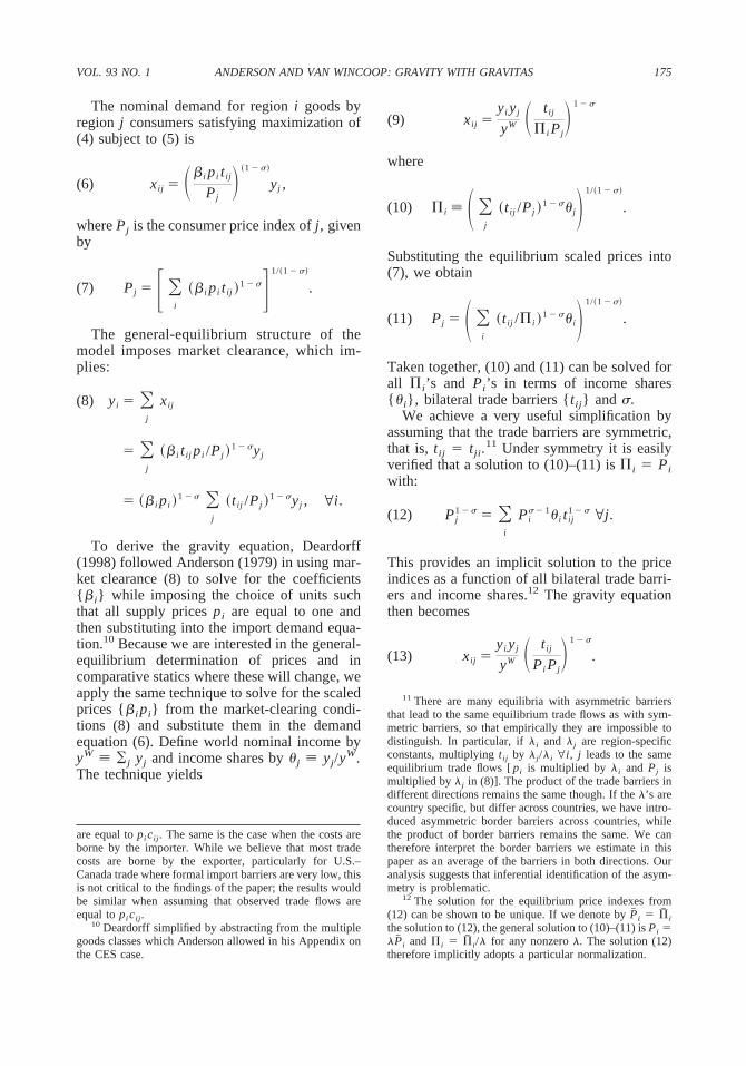
The nominal demand for region i goods byregion j consumers satisfying maximization of(4) subject to (5) is

(6) xij � �� i pi tij

Pj� �1 � ��

yj ,

where Pj is the consumer price index of j, givenby

(7) Pj � � �i

�� i pi tij �1 � �� 1/�1 � ��

.

The general-equilibrium structure of themodel imposes market clearance, which im-plies:

(8) yi � �j

xij

� �j

�� i t ij pi /Pj �1 � �yj

� �� i pi �1 � � �

j

�tij /Pj �1 � �yj , @i.

To derive the gravity equation, Deardorff(1998) followed Anderson (1979) in using mar-ket clearance (8) to solve for the coefficients{�i} while imposing the choice of units suchthat all supply prices pi are equal to one andthen substituting into the import demand equa-tion.10 Because we are interested in the general-equilibrium determination of prices and incomparative statics where these will change, weapply the same technique to solve for the scaledprices {�ipi} from the market-clearing condi-tions (8) and substitute them in the demandequation (6). Define world nominal income byyW � ¥j yj and income shares by �j � yj/y

W.The technique yields

(9) xij �yi yj

yW � tij

� i Pj� 1 � �

where

(10) � i � � �j

�tij /Pj �1 � �� j� 1/�1 � ��

.

Substituting the equilibrium scaled prices into(7), we obtain

(11) Pj � � �i

�tij /� i �1 � �� i� 1/�1 � ��

.

Taken together, (10) and (11) can be solved forall �i’s and Pi’s in terms of income shares{�i}, bilateral trade barriers {tij} and �.

We achieve a very useful simplification byassuming that the trade barriers are symmetric,that is, tij � tji.

11 Under symmetry it is easilyverified that a solution to (10)–(11) is �i � Piwith:

(12) Pj1 � � � �

i

Pi� � 1� i t ij

1 � � @j.

This provides an implicit solution to the priceindices as a function of all bilateral trade barri-ers and income shares.12 The gravity equationthen becomes

(13) xij �yi yj

yW � tij

Pi Pj� 1 � �

.

are equal to picij. The same is the case when the costs areborne by the importer. While we believe that most tradecosts are borne by the exporter, particularly for U.S.–Canada trade where formal import barriers are very low, thisis not critical to the findings of the paper; the results wouldbe similar when assuming that observed trade flows areequal to picij.

10 Deardorff simplified by abstracting from the multiplegoods classes which Anderson allowed in his Appendix onthe CES case.

11 There are many equilibria with asymmetric barriersthat lead to the same equilibrium trade flows as with sym-metric barriers, so that empirically they are impossible todistinguish. In particular, if i and j are region-specificconstants, multiplying tij by j/i @i, j leads to the sameequilibrium trade flows [ pi is multiplied by i and Pj ismultiplied by j in (8)]. The product of the trade barriers indifferent directions remains the same though. If the ’s arecountry specific, but differ across countries, we have intro-duced asymmetric border barriers across countries, whilethe product of border barriers remains the same. We cantherefore interpret the border barriers we estimate in thispaper as an average of the barriers in both directions. Ouranalysis suggests that inferential identification of the asym-metry is problematic.

12 The solution for the equilibrium price indexes from(12) can be shown to be unique. If we denote by P� i � �� i

the solution to (12), the general solution to (10)–(11) is Pi �P� i and �i � �� i/ for any nonzero . The solution (12)therefore implicitly adopts a particular normalization.


Our basic gravity model is (13) subject to (12).Equation (13) significantly simplifies expres-sions derived by Anderson (1979) and Dear-dorff (1998), while our simultaneous use of themarket-clearing constraints to obtain the equi-librium price indexes in (12) is a significant inno-vation that will allow us to estimate the gravityequation and therefore make it operational.

We will refer to the price indices {Pi} as“multilateral resistance” variables as they de-pend on all bilateral resistances {tij}, includingthose not directly involving i. A rise in tradebarriers with all trading partners will raise theindex. For example, in the absence of trade barri-ers (all tij � 1) it follows immediately from (12)that all price indices are equal to 1. Below we willshow that a marginal increase in cross-countrytrade barriers will raise all price indices above 1.

While the Pi are consumer price indices inthe model, that would not be a proper interpre-tation of these indices more generally. One canderive exactly the same gravity equation andsolution to the Pi when trade costs are nonpe-cuniary. An example is home bias in prefer-ences, whereby cij in the utility function isreplaced by cij/tij. In that case Pi no longerrepresents the consumer price index and theborder barrier includes home bias.

The gravity equation tells us that bilateraltrade, after controlling for size, depends on thebilateral trade barrier between i and j, relativeto the product of their multilateral resistanceindices. It is easy to see why higher multilateralresistance of the importer j raises its trade withi. For a given bilateral barrier between i and j,higher barriers between j and its other tradingpartners will reduce the relative price of goodsfrom i and raise imports from i. Higher multi-lateral resistance of the exporter i also raisestrade. Higher trade barriers faced by an exporterwill lower the demand for its goods and there-fore its supply price pi. For a given bilateralbarrier between i and j, this raises the level oftrade between them.

The gravity model (13), subject to (12), im-plies that bilateral trade is homogeneous of de-gree zero in trade costs, where these include thecosts of shipping within a region, tii. This fol-lows because the equilibrium multilateral resis-tances Pi are homogeneous of degree 1⁄2 in thetrade costs. The economics behind the formalresult is that the constant vector of real productsmust be distributed despite higher trade costs.

The rise in trade costs is offset by the fall insupply prices [they are homogeneous of degreeminus 1⁄2 in trade costs, based on (7) and thehomogeneity of the equilibrium multilateral re-sistances] required to achieve shipment of thesame volume. The invariance of trade to uni-form decreases in trade costs may offer a clue asto why the usual gravity model estimation hasnot found trade becoming less sensitive to dis-tance over time (Barry Eichengreen and Doug-las A. Irwin, 1998).

The key implication of the theoretical gravityequation is that trade between regions is deter-mined by relative trade barriers. Trade betweentwo regions depends on the bilateral barrierbetween them relative to average trade barriersthat both regions face with all their tradingpartners. This insight has many implications forthe impact of trade barriers on trade flows. Herewe will focus on one important set of implica-tions related to the size of countries becausethey are useful in interpreting the findings inSection IV. Consider the simple thought exper-iment of a uniform rise in border barriers be-tween all countries. For simplicity we assumethat each region i is a frictionless country. Wewill discuss three general-equilibrium compar-ative static implications of this experiment,which are listed below.

IMPLICATION 1: Trade barriers reduce size-adjusted trade between large countries morethan between small countries.

IMPLICATION 2: Trade barriers raise size-adjusted trade within small countries more thanwithin large countries.

IMPLICATION 3: Trade barriers raise theratio of size-adjusted trade within country 1relative to size-adjusted trade between coun-tries 1 and 2 by more the smaller is country 1and the larger is country 2.

The experiment amounts to a marginal in-crease in trade barriers across all countries, sodtij � dt, i � j; dtii � 0. Frictionless initialequilibrium implies tij � 1 @i, j f Pi � 1.Differentiating (12) at tij � 1, @i, j yields13

13 To obtain this expression we differentiate totally attij � 1 � Pi to obtain


(14) dPi � � 12

� i �12 �

k

�k2�dt.

Thus a uniform increase in trade barriers raisesmultilateral resistance more for a small countrythan a large country.14 In a two-country exam-ple, where the small country’s income is 10percent of the total, a 20-percent trade barrierraises the price index of the large country by 0.2percent, while raising the price index of thesmall country by 16 percent. This is not unlikethe U.S.–Canada example to which the modelwill be applied later. For a very large countrymultilateral resistance is not much affected be-cause increased trade barriers do not apply totrade within the country. For a small countrytrade is more important and trade barriers there-fore have a bigger effect on multilateral resistance.

Equation (14) implies that the level of tradebetween countries i and j, after controlling forsize, changes by

(15)

d� xij

yW

yi yj� � �� 1��i � �j �k

�k2�dt.

This implies that trade between large countriesdrops more than trade between small countries(Implication 1). While two small countries facea larger bilateral trade barrier, they face thesame increase in trade barriers with almost theentire world. Bilateral trade depends on the rel-ative trade resistance tij/PiPj. Since multilateraltrade resistance rises much more for small coun-tries than for large countries, relative trade re-

sistance rises less for small countries, so thattheir bilateral trade drops less.15

Equation (14) also implies that trade within acountry i, after controlling for size, increases by

(16)

d� xii

yW

yi yi� � �� 1��1 2� i � �k

�k2�dt.

Therefore trade within a small country increasesmore than trade within a large country (Implica-tion 2). A rise in multilateral resistance implies adrop in relative resistance tii/PiPi for intranationaltrade. The drop is larger for small countries thatface a bigger increase in multilateral resistance.

Implication 3 follows from the previous two.After controlling for size, trade within country irelative to trade between countries i and j rises by

(17) d� xii /yi yi

xij /yi yj� � �� 1�1 � i � � j dt.

The increase is larger the smaller i and thebigger j. We already knew from Implication 2that intranational trade rises most for smallcountries. From Implication 1 we also knowthat for a given small country international tradedrops most with large countries.

The implications relating to size are muchmore general than the specifics of the modelmight suggest. Consider the following examplewithout any reference to gravity equations andmultilateral resistance variables. A small econ-omy with two regions and a large economy with100 regions engage in international trade. Allregions have the same GDP. What matters hereis not the number of regions, but the relativesize of the two economies as measured by totalGDP. We only introduce regions in this exam-ple because it is illustrative in the context of theU.S. states and Canadian provinces that are thefocus of the empirical analysis. Under borderless

dPj � �i

� i dtij �i

� i dPi �1

1 � �i

d� i .

¥i d�i � 0, since the sum of the shares is equal to one.Multiplying each equation by �j and summing using dtij �dt, i � j, dtii � 0, we solve for ¥ �jdPj � (1 � ¥�j

2)dt/ 2 and thus dPi � (1⁄2 � �i � ¥ �j2/ 2)dt.

14 Country size is determined by the endowment of thegoods. It can be shown that at the frictionless equilibrium, arise in country i’s endowment will lower its supply price pi ,raise all other supply prices, and with � � 1 this will raise�i and lower the other income shares. Thus we treat �i as anexogenous variable for the purposes of talking about coun-try size.

15 As is immediately clear from (15), trade between twosmall countries can even rise after a uniform increase intrade barriers. This is because the pre-barrier prices pi dropmore in small countries than in large countries as smallcountries are more affected by a drop in foreign demand.This makes it more attractive for small countries to tradewith each other than with large countries.


trade, all regions sell one unit of one good to all102 regions (including themselves). Now im-pose a barrier between the small and the largecountry, reducing trade between the two coun-tries by 20 percent. Region 1 in the small coun-try then reduces its exports to the large countryby 20. It sells ten more goods to itself and tenmore goods to region 2 in the small country.Trade between the two regions in the smallcountry rises by a factor 11, while trade be-tween two regions in the large country rises bya factor of only 1.004 (an illustration of Impli-cation 2 above). This shows that even a smalldrop in international trade can lead to a verylarge increase in trade within a small country.Trade between the two regions in the smallcountry is now 13.75 times trade between re-gions in both countries, while trade betweentwo regions in the large country is only 1.255times trade between regions in the two countries(an illustration of Implication 3).

The final step in our theoretical developmentof the gravity equation is to model the unob-servable trade cost factor tij. We follow otherauthors in hypothesizing that tij is a loglinearfunction of observables, bilateral distance dij ,and whether there is an international borderbetween i and j:

(18) tij � bij dij� .

bij � 1 if regions i and j are located in the samecountry. Otherwise bij is equal to one plus thetariff equivalent of the border barrier betweenthe countries in which the regions are located.Other investigators have added other factorsrelated to trade barriers, such as adjacency andlinguistic identity. We have chosen the trade costsspecification (18) to stay as close as possible toMcCallum’s (1995) equation, so that we can keepthe focus on the multilateral resistance indices thatare absent from McCallum’s analysis.

We can now compare the theoretical gravityequation with that estimated in the empiricalliterature. The theory implies that

(19)

ln xij � k � ln yi � ln yj � �1 �� ln dij

� �1 ��ln bij �1 ��ln Pi

� �1 ��ln Pj

where k is a constant. The key difference be-tween (20) and equation (1) estimated by Mc-Callum is the two price index terms. Theomitted multilateral resistance variables arefunctions of all bilateral trade barriers tijthrough (12), which in turn are a function of dijand bij through the trade cost equation (18).Since the multilateral resistance terms are there-fore correlated with dij and bij , they createomitted variable bias when the coefficient of thedistance and border variables is interpreted as(1 � �)� and (1 � �)ln bij. Our multilateralresistance variables bear some resemblance to“remoteness” indexes such as (3) that have beenincluded in gravity equation estimates subse-quent to McCallum’s paper. But the latter donot include border barriers and even withoutborder barriers the functional form is entirelydisconnected from the theory. Finally, our mul-tilateral resistance variables as equilibrium con-structs are functions of all bilateral resistancesin the solution to (12).

A small difference between the theory andthe empirical literature is that the theoreticalgravity equation imposes unitary income elas-ticities. Anderson (1979) provided a rationalefor earlier (and subsequent) empirical gravitywork that estimates nonunitary income elastic-ities. He allowed for nontraded goods andassumed a reduced-form function of the expen-diture share falling on traded goods as a func-tion of total income. We already found inSection I that imposing unitary income elastic-ities has little effect on McCallum’s border es-timates. We will therefore impose unitaryincome elasticities in most of the analysis, leav-ing an extension to nonunitary elasticities tosensitivity analysis.

III. Estimation

We implement the theory both in the contextof a two-country model, consisting of theUnited States and Canada, and a multicountrymodel that also includes other industrializedcountries. The latter approach is obviously morerealistic as it takes into account that the UnitedStates and Canada also trade with other coun-tries. It has the additional advantage that itdelivers an estimate of the impact of borderbarriers on trade among the other industrializedcountries. We first discuss the two-countrymodel and then the multicountry model.


A. Two-Country Model

In the two-country model we estimate thegravity equation for trade flows among the same30 states and 10 provinces as in McCallum(1995). We do not include in the sample theother 21 regions (20 states plus the District ofColumbia), which account for about 15 percentof U.S. GDP, and trade flows internal to a stateor province. However, in order to compute themultilateral resistance variables for the regionsin our sample, we do need to use information onsize and distance associated with the other 21regions and we also need to use information onthe distances within regions. We simplify byaggregating the other 21 regions into one re-gion, defining the distance between this regionand region i in our sample as the GDP weightedaverage of the distance between i and each ofthe 21 regions that make up the new region.There is no obvious way to compute distancesinternal to a region. Fortunately, as we willshow in Section V, our results are not verysensitive to assumptions about internal distance.We use the proxy developed by Wei (1996),which is one-fourth the distance of a region’scapital from the nearest capital of anotherregion.16

In the two-country model bij � b1 � �ij ,where b � 1 represents the tariff-equivalentU.S.–Canada border barrier and �ij is the samedummy variable as in Section I, equal to one ifi and j are in the same country and zerootherwise.

We estimate a stochastic form of (13):

(20) ln zij � ln� xij

yi yj�

� k � a1ln dij � a2 �1 �ij �

� ln Pi1 � � ln Pj

1 � � � �ij

where a1 � (1 � �)� and a2 � (1 � �)ln b.To stay as close as possible to McCallum’s(1995) regression we have simply added an

error term to the logarithmic form of the gravityequation, which one can think of as reflectingmeasurement error in trade. Apart from the uni-tary income elasticities, the only difference withMcCallum (1995) is the presence of the twomultilateral resistance terms.

The multilateral resistance terms are not ob-servables. As discussed above, the price indicesin general cannot be interpreted as consumerprice levels.17 The observables in our model aredistances, borders, and income shares. Usingthe 41 goods market-equilibrium conditions(12) and the trade cost function (18), we cansolve for the vector of the Pi

1�� as an implicitfunction of observables and model parametersa1 and a2:

(21) Pj1 � � � �

i

Pi� � 1� i e

a1ln dij�a2 �1��ij �

j � 1, ... , 41.

After substituting the implicit solutions for thePi

1�� in (21), the gravity equation to be esti-mated becomes:

(22) ln z � h�d, �, �; k, a1 , a2 � � �

where z, d, �, �, and � are vectors that containall the elements of the corresponding variableswith subscripts, and h� is the right-hand sideof (20) after substituting the equilibrium Pi

1��

and Pj1��.

The right-hand side is now written explicitlyas a function of observables. We estimate (22)with nonlinear least squares, minimizing thesum of squared errors. For any set of parametersthe error terms of the regression can only becomputed after first solving for 41 equations(21). The estimated parameters are k, a1, and

16 For the region obtained from the aggregation of the 21regions, we compute internal distance as ¥i�1

21 ¥j�121 si sjdij ,

where si is the ratio of GDP in region i to total GDP of the21-region area.

17 Even if one assumes that the price indices are con-sumer price levels, which would require that all trade costsare pecuniary costs, there are still many measurement prob-lems that makes them unobservable for our purposes. Non-traded goods, which are not present in our model, play a keyrole in explaining differences in price levels across coun-tries and regions. In the short to medium run, nominalexchange rates also have a significant impact on the ratio ofprice levels across countries. Moreover, while comparableprice-level data are available for countries, this is not thecase for states and provinces.


a2.18 The substitution elasticity � cannot beestimated separately as it enters in multiplica-tive form with the trade cost parameters � andln b in a1 and a2.19

Our estimator is unbiased if � is uncorrelatedwith the derivatives of h with respect to d, �,and �. This is not a problem when we interpret�ij simply as measurement error associated withbilateral trade, as we have done. Errors canenter the model in many other ways of course,about which the theory has little to say. Inparticular, it is possible that the trade cost func-tion (18) is misspecified in that other factorsthan just distance and borders matter, or thefunctional form is incorrect. One could add anerror term to the trade cost function to capturethis. If this error term is correlated with d or �,our estimates will be biased. But this is a stan-dard omitted variables problem that is not spe-cific to the presence of multilateral resistanceterms. We have chosen the trade cost functionto stay as close as possible to McCallum’s(1995) specification. If an error term in the tradecost function is uncorrelated with d and �, thereis still the problem that the error term affectsequilibrium prices and therefore income shares�, which affect the multilateral resistance terms.In practice the bias resulting from this is verysmall though. As we will report below, even ifwe take the dramatic step of entirely removingthe U.S.–Canada border, practically none of theresulting changes in the Pi

1�� are associatedwith changes in income shares.

An alternative to the estimation method de-scribed above is to replace the multilateral re-sistance terms with country-specific dummies.This leads to consistent estimates of model pa-rameters. Hummels (1999) has done so for agravity equation using disaggregated U.S. im-port data. The main advantage is simplicity as

ordinary least squares can be used. Anotheradvantage is that we do not need to make anyassumptions about distances internal to statesand provinces, which are needed to compute thestructural multilateral resistance terms and aredifficult to measure. Rose and van Wincoop(2001) use this estimator when applying themethod in this paper to determine the effect ontrade of monetary unions. We need to empha-size though that the fixed-effects estimator isless efficient than the nonlinear least-squaresestimator discussed above, which uses informa-tion on the full structure of the model. Thesimple fixed-effects estimator is not necessarilymore robust to specification error. For example,if the trade cost function is misspecified, eitherin terms of functional form or set of variables,both estimators are biased to the extent that thespecification error is correlated with distance orthe border dummy.

For comparative statics analysis, such as re-moving the U.S.–Canada border, the structuralmodel can be used with either method of esti-mation. We use the fixed-effects estimator insensitivity analysis reported in Table 6, givingsimilar results.

B. Multicountry Model

In the multicountry model the world consistsof all industrialized countries, a total of 22countries.20 In that case there are 61 regions inour analysis: 30 states, the rest of the UnitedStates, 10 provinces, and 20 other countries. Wewill often refer to the 20 additional countries asROW (rest of the world). In this expanded en-vironment we assume that border barriers bijmay differ for U.S.–Canada trade, US–ROWtrade, Canada–ROW trade, and ROW–ROWtrade. We define these respectively as bUS,CA,bUS,ROW, bCA,ROW, and bROW,ROW.

For consistency with the estimation methodin the two-country model, and given our focuson the U.S.–Canada border effect, we will con-tinue to estimate the parameters by minimizingthe sum of the squared residuals for the 30 statesand 10 provinces. But there are now three ad-

18 Computationally, we solve

mink,a1 ,a2

�i

�j�i

ln zij k a1ln dij a2 �1 �ij �

� ln Pi1 � � � ln Pj

1 � �]2

subject to Pj1 � � � �

i

Pi� � 1�i e

a1ln dij�a2 �1��ij � @j.

19 As Hummels (1999) has shown, identification of � ispossible in applications where elements of tij are directlyobservable, as with tariffs.

20 Those are the United States, Canada, Australia, Japan,New Zealand, Austria, Belgium-Luxembourg, Denmark,Finland, France, Germany, Greece, Ireland, Italy, Nether-lands, Norway, Portugal, Spain, Sweden, Switzerland, andthe United Kingdom.


ditional parameters that affect the multilateralresistance variables of the states and provinces:(1 � �)ln bUS,ROW, (1 � �)ln bCA,ROW, and(1 � �)ln bROW,ROW. We impose three con-straints in order to obtain estimates for theseparameters. The constraints set the average ofthe residuals for US–ROW trade, CA–ROWtrade, and ROW–ROW trade equal to zero.21

Formally,

�j�ROW

��US,j � � j,US � � 0

�j�ROW

��CA,j � � j,CA � � 0

�i,j�ROW

�i�j

� ij � 0.

Since we have data on trade only between theROW countries and all of the United States, theresiduals �US, j and �j,US are defined as the logof bilateral trade between the United States andcountry j minus the log of predicted trade,where the latter is obtained by summing overthe model’s predicted trade between j and allU.S. regions. The same is done for trade be-tween Canada and countries in ROW.22

IV. Results

Our goal in this section is threefold. First, wereport results from estimating the theoreticalgravity equation. Second, we use the estimatedgravity equation to determine the impact ofnational borders on trade flows. This is done bycomputing the change in bilateral trade flowsafter removing the border barriers. Finally, weuse the estimated gravity equation to accountfor the estimated McCallum border parame-ters. This procedure illustrates the role of themultilateral resistance variables in generatinga much smaller McCallum border parameterfor the United States than for Canada as wellas the effect of the omitted variable bias inMcCallum’s procedure.

A. Parameter Estimates

Table 2 reports the bilateral trade resistanceparameter estimates. The estimate of the U.S.–Canada border barrier is very similar in both thetwo-country model and the multicountry model.In the multicountry model the border barrierestimates are also strikingly similar acrosscountry pairs. The barrier between the UnitedStates and Canada is only slightly lower thanbetween the other 20 industrialized countries,the majority of which is trade among EuropeanUnion countries. The only border barrier that isa bit higher than the others is between Canadaand the ROW countries.

As discussed above, we can estimate only(1 � �)ln b. We would need to make an as-sumption about the elasticity of substitution �in order to obtain an estimate of b � 1, the advalorem tariff equivalent of the border barrier.The model is of course highly stylized in thatthere is only one elasticity. In reality somegoods may be perfect substitutes, with an infi-nite elasticity, while others are weak substitutes.Hummels (1999) obtains estimates for the elas-ticity of substitution within industries. The re-sults depend on the disaggregation of theindustries. The average elasticity is respectively4.8, 5.6, and 6.9 for 1-digit, 2-digit, and 3-digit

21 Apart from consistency with the two-country estima-tion method, there are two reasons why we prefer thisestimation method as opposed to minimizing the sum of allsquared residuals, including those of the ROW countries.First, border barriers are likely to be different across countrypairs for the 20 other industrialized countries. Neither esti-mation method allows us to identify all these barriers sep-arately, but the method we chose is less sensitive to suchdifferences as we only use information on the average errorterms involving the ROW countries. Second, the alternativemethod of minimizing the sum of all squared residuals hasweaker finite sample properties. The US–ROW barrier hasa much greater impact on US–ROW trade than on tradeamong the states and provinces, but US–ROW observationsare only 2 percent of the sample. If there is only weakspurious correlation between the 1,511 error terms for tradeamong states and provinces and the partial derivatives of thecorresponding multilateral resistance terms with respect tothe US–ROW barrier, it could significantly affect the esti-mate of that barrier.

22 Data on exports from individual states to ROW coun-tries do exist (see Robert C. Feenstra, 1997), but this isbased on information about the location of the exporter,which is often not the location of the plant where the goodsare produced. The International Trade Division and theInput Output Divisions of Statistics Canada both report dataon trade between provinces and the rest of the world. Thedata from the IO Division are considered more reliable, but

only the IT division reports trade with individual countries.The differences between the total export and import num-bers reported by both divisions are often very large (almosta factor 8 difference for imports by Prince Edward Island).


industries. For further levels of disaggrega-tion the elasticities could be much higher, withsome goods close to perfect substitutes.23 Itis therefore hard to come up with an appro-priate average elasticity. To give a sense ofthe numbers though, the estimate of �1.58 for(1 � �)ln bUS,CA in the multicountry modelimplies a tariff equivalent of respectively 48,19, and 9 percent if the average elasticity is 5,10, and 20.

The last three rows of Table 2 report theaverage error terms for interstate, interprovin-cial, and state–province trade. Particularly forthe multicountry model they are close to zero.The average percentage difference between ac-tual trade and predicted trade in the multicoun-try model is respectively 6, �2, and �4 percentfor interstate, interprovincial, and state–provincetrade. The largest error term in the two-countrymodel is for interprovincial trade, where onaverage actual trade is 17 percent lower thanpredicted trade.24

B. The Impact of the Borderon Bilateral Trade

We now turn to the general-equilibrium com-parative static implications of the estimated bor-der barriers for bilateral trade flows. We willcalculate the ratio of trade flows with borderbarriers to that under the borderless trade im-plied by our model estimates. Appendix B dis-cusses how we compute the equilibrium afterremoving all border barriers while maintainingdistance frictions. It turns out that we need toknow the elasticity � in order to solve for thefree trade equilibrium. This is because the newincome shares �i depend on relative prices,which depend on �. We set � � 5, but we willshow in the sensitivity analysis section that re-sults are almost identical for other elasticities.The elasticity � plays no role other than toaffect the equilibrium income shares a little.

In what follows we define the “average” oftrade variables and (transforms of the) multilat-eral resistance variables as the exponential of

23 For example, for a highly homogeneous commoditysuch as silver bullion, Feenstra (1994) estimates a 42.9elasticity of substitution among varieties imported from 15different countries.

24 The R� 2 is respectively 0.43 and 0.45 for the two-country and multicountry model, which is somewhat lowerthan the 0.55 for the McCallum equation with unitary elas-ticities (last column Table 1). This is not a test of the theorythough because McCallum’s equation is not theoreticallygrounded. It also does not imply that multilateral resistance

does not matter; the dummies in McCallum’s equationcapture the average difference in multilateral resistance ofstates and provinces. With a higher estimate of internaldistance, the R� 2 from the structural model becomes quiteclose to that in the McCallum equation. It turns out thoughthat internal distance has little effect on our key results(Section V).

TABLE 2—ESTIMATION RESULTS

Two-countrymodel

Multicountrymodel

Parameters (1 � �)� �0.79 �0.82(0.03) (0.03)

(1 � �)ln bUS,CA �1.65 �1.59(0.08) (0.08)

(1 � �)ln bUS,ROW �1.68(0.07)

(1 � �)ln bCA,ROW �2.31(0.08)

(1 � �)ln bROW,ROW �1.66(0.06)

Average error terms: US–US 0.06 0.06CA–CA �0.17 �0.02US–CA �0.05 �0.04

Notes: The table reports parameter estimates from the two-country model and the multicoun-try model. Robust standard errors are in parentheses. The table also reports average errorterms for interstate, interprovincial, and state–province trade.


the average logarithm of these variables, con-sistent with McCallum (1995).25

The multilateral resistance variables are crit-ical to understanding the impact of border bar-riers on bilateral trade and understanding whataccounts for the McCallum border parameters.Defining regions in the United States, Canada,and ROW as three sets, Table 3 reports theaverage transform of multilateral resistanceP� � 1 for regions in each of these sets. Theresults are shown both with the estimated borderbarrier and under borderless trade. As discussedin Section II, based on the model we wouldexpect border barriers to lead to a larger in-crease of multilateral resistance in small coun-tries than in large countries. This is exactly whatwe see in Table 3. P� � 1 rises by 12 percent forU.S. states, while it rises by a factor 2.44 forCanadian provinces.26 The number is interme-diate for ROW countries, whose size is also

intermediate. The Canadian border creates abarrier between provinces and most of its po-tential trading partners, while states face noborder barriers with the rest of the large U.S.economy. Multilateral resistance therefore risesmuch more for provinces than for states.

Even under borderless trade Pi1�� is substan-

tially higher for provinces than for states. Dis-tances are somewhat larger on average betweenthe United States and Canada than within them.This affects multilateral resistance for provincesmore than for states as most potential tradingpartners of the provinces are outside their coun-try, while for the states they are inside thecountry. This is again the result of the small sizeof the Canadian economy.

Table 3 reports the transforms Pi1�� of the

multilateral resistance indices because theymatter for trade levels. It is worthwhile pointingout that the Pi themselves, which are a measureof average trade barriers faced by regions, risemuch less as a result of borders. For � � 5, Pirises on average by 3 percent for states and 25percent for Canadian provinces. For higher � itis even smaller.

Table 4 reports the impact of border barrierson bilateral trade flows among and within eachof the three sets of regions (US, CA, ROW).Size is controlled for by multiplying the bilat-eral trade numbers by yW/( yiyj). Letting a tildedenote borderless trade, the ratio of averagetrade between regions in sets h and k (h, k �US, CA, ROW) with and without border bar-riers is

(23) bhk1 � ��Ph

� � 1

Ph� � 1��Pk

� � 1

Pk� � 1�

where Ph��1 refers to the average of regions in

that set. We can therefore break down the im-pact of border barriers on trade into the impactof the bilateral border barrier and the impact ofborder barriers on multilateral resistance of re-gions in both sets. To the extent that borderbarriers raise average trade barriers faced by animporter and an exporter (multilateral resis-tance), it dampens the negative impact of thebilateral border barrier on trade between the two

25 McCallum’s border effect is the difference betweenthe average logarithm of bilateral trade among regions in thesame country and the average logarithm of bilateral trade ofregions in different countries. This is converted back tolevels by taking the exponential. Among a set of regions,bilateral trade between two regions is therefore consideredto be average when the logarithm of bilateral trade is aver-age within the set.

26 Very little of the change in P� � 1 is associated with achange in income shares �i. The change in income shares

alone would lower P� � 1 for Canadian provinces by 0.4percent and raise it for states by 0.8 percent.

TABLE 3—AVERAGE OF P1 � �

US Canada ROW

Two-country model

With border barrier (BB) 0.77 2.45(0.03) (0.12)

Borderless trade (NB) 0.75 1.18(0.03) (0.01)

Ratio (BB/NB) 1.02 2.08(0.00) (0.08)

Multicountry model

With border barrier (BB) 1.55 4.67 2.97(0.01) (0.09) (0.07)

Borderless trade (NB) 1.39 1.91 1.54(0.00) (0.04) (0.01)

Ratio (BB/NB) 1.12 2.44 1.93(0.01) (0.09) (0.06)

Notes: The table reports the average of Pi��1, where the

average is defined as the exponential of the average loga-rithm. For the United States the average is taken over the 30states in the sample, for Canada over the 10 provinces, andfor ROW over the other 20 industrialized countries.


countries. In what follows we will focus on thenumbers for the more realistic multicountrymodel.

Implication 2 of the theory that cross-countrytrade barriers raise trade within a country morefor small than for large countries is stronglyconfirmed in Table 4. The table reports a spec-tacular factor 6 increase in interprovincial tradedue to borders, while interstate trade rises byonly 25 percent. The larger increase in multilat-eral resistance of the provinces leads to a biggerdrop in relative trade resistance tii/PiPi fortrade within Canada than within the UnitedStates, explaining the large increase in interpro-vincial trade.

Table 4 also reports that borders reduce tradebetween the United States and Canada to afraction 0.56 of that under borderless trade, orby 44 percent. Trade among ROW countries isreduced by 29 percent. The bilateral border bar-rier itself implies an 80-percent drop in tradebetween states and provinces, but increasedmultilateral resistance, particularly for prov-inces, raises state–province trade by a factor 2.72.While U.S. goods have become more expensivefor Canada due to the border barrier, the goods ofalmost all trading partners of the provinces havebecome more expensive. This significantly mod-erates the negative impact on U.S.–Canada trade.

It may seem somewhat surprising that tradebetween the ROW countries drops somewhat

less than between the United States and Canada,particularly because the estimates in Table 2 im-ply a slightly lower U.S.–Canada border barrier.But it can be understood in the context of Im-plication 1 from the theory that border barriershave a bigger effect on trade between countriesthe larger their size. For the same border barri-ers, U.S.–Canada trade would have droppedmuch less if the United States were a muchsmaller country. This also explains why tradebetween the United States and the ROW coun-tries drops somewhat more than between theUnited States and Canada. Canada is evensmaller than the average ROW country. Basedon size alone one would expect trade betweenCanada and the ROW countries to drop lessthan between Canada and the United States, butthis is not the case as a result of the higher tradebarrier between Canada and the ROW countries.

C. Intranational Trade Relative toInternational Trade

McCallum aimed to measure the impact ofborders on intranational trade (within Canada)to international trade (between the United Statesand Canada). In this subsection we will showthat the large McCallum border parameter forCanada is due to a combination of (i) the rela-tive small size of the Canadian economy and (ii)omitted variables bias.

TABLE 4—IMPACT OF BORDER BARRIERS ON BILATERAL TRADE

US–US CA–CA US–CA US–ROW CA–ROW ROW–ROW

Two-country model

Ratio BB/NB 1.05 4.31 0.41(0.01) (0.34) (0.02)

Due to bilateral resistance 1.0 1.0 0.19(0.0) (0.0) (0.01)

Due to multilateral resistance 1.05 4.31 2.13(0.01) (0.34) (0.09)

Multicountry model

Ratio BB/NB 1.25 5.96 0.56 0.40 0.46 0.71(0.02) (0.42) (0.03) (0.01) (0.01) (0.02)

Due to bilateral resistance 1.0 1.0 0.20 0.19 0.10 0.19(0.0) (0.0) (0.02) (0.01) (0.01) (0.01)

Due to multilateral resistance 1.25 5.96 2.72 2.15 4.70 3.71(0.02) (0.42) (0.12) (0.09) (0.31) (0.25)

Notes: The table reports the ratio of trade with the estimated border barriers (BB) to that under borderless trade (NB). Thisratio is broken down into the impact of border barriers on trade through bilateral resistance (tij

1��) and through multilateralresistance (Pi

��1Pj��1).


The impact of border barriers on intranationalrelative to international trade follows immedi-ately from Table 4 and is reported in the firstrow of Table 5. The multicountry model impliesthat national borders lead to trade between prov-inces that is a factor 10.7 larger than betweenstates and provinces. In contrast, border barriersraise trade between states by only a factor 2.24relative to trade between states and provinces.This is exactly as anticipated by Implication 3of the theory. It is the result of the relativelysmall size of Canada, leading to a factor 6increase in trade between the provinces. Thesmall change in trade between U.S. states leadsto a correspondingly much smaller increase inintranational to international trade for theUnited States.

This is only part of the explanation for thelarge McCallum border parameter for Canada.The other part is the result of omitted variablesbias in two distinct senses: estimation and com-putation. By estimation bias we mean the ordi-nary econometric omitted variables bias. Bycomputation bias we mean the erroneous com-parative statics which arise from a reduced-formcalculation which omits terms. In order to ana-lyze the omitted variables bias, rewrite the the-oretical gravity equation as

(24) ln xij � k � ln yi � ln yj

� ��1 ��ln dij � Rij � �ij

where

Rij � �1 ��ln bij �1 ��ln Pi

� �1 ��ln Pj .

Rij measures the sum of all trade resistanceterms with the exception of the bilateral dis-tance term. McCallum estimated (24), but re-placed Rij with a dummy variable that is 1 forinterprovincial trade and 0 for state–provincetrade. In the absence of the multilateral resis-tance terms this would yield unbiased estimatesof (1 � �)� and (1 � �)ln b. But since theomitted multilateral resistance terms are corre-lated with both distance and the border dummy,McCallum’s regression does not yield an unbi-ased estimate of either (1 � �)� or (1 � �)ln b.Next, consider computation bias. Assume forthe moment that McCallum had correctly esti-mated the parameter (1 � �)� multiplying bi-lateral distance. In that case McCallum’s bordereffect can still not be interpreted as the effect ofborders on the ratio of interprovincial trade rel-ative to state–province trade. In the context ofthe theory we can then interpret McCallum’sborder parameter for Canada as an estimator ofthe average of Rij for interprovincial trade mi-nus the average for state–province trade, andsimilarly for the United States.27 Taking theexponential for comparison with McCallum’sheadline number, we get (following the notationof Section I)

(25) BorderCanada � �bUS,CA �� 1PCA

� � 1

PUS� � 1 .

27 We will take the average over all trade pairs, eventhough for a few state–province pairs and state–statepairs no trade data exist. Taking the average only overpairs for which trade data exist leads to almost identicalnumbers.

TABLE 5—IMPACT BORDER ON INTRANATIONAL TRADE RELATIVE TO INTERNATIONAL TRADE

Two-country model Multicountry model

Canada US Canada US

Theoretically consistent estimate 10.5 2.56 10.7 2.24(1.16) (0.13) (1.06) (0.12)

McCallum parameter implied by theory 16.5 1.64 14.8 1.63(1.63) (0.09) (1.32) (0.10)

Notes: The first row of the table reports the theoretically consistent estimate of the impact ofborder barriers on intranational trade relative to international trade for both Canada and theUnited States. The second row reports the McCallum border parameter implied by the model,which provides a biased estimate of the impact of borders on the ratio of intranational tointernational trade.


Similarly, for the United States we get

(26) BorderUS � �bUS,CA �� 1PUS

� � 1

PCA� � 1 .

The theoretical McCallum border parametersimplied by (25)–(26) are reported in the secondrow of Table 5. For the multicountry model theborder parameters are 14.8 for Canada and 1.63for the United States. This corresponds closelyto the 14.2 and 1.62 parameters reported in the lastcolumn of Table 1 when estimating McCallum’sregression with unitary income coefficients. Themuch higher Canadian (transform of) multilat-eral resistance term, PCA

��1, than the U.S. mul-tilateral resistance term, PUS

��1, blows up theborder effect for Canada, while dampening itwith the same factor for the United States.

A comparison of rows 1 and 2 of Table 5shows that McCallum’s measure for Canadaoverstates our consistent estimate of the impactof borders on intranational trade relative to in-ternational trade. The reason is that in the cor-rect measure of the impact of borders onintranational relative to international trade, themultilateral resistance terms in (25) and (26) arereplaced by the ratio of multilateral resistancewith border barriers relative to that without bor-der barriers; the comparative static experimentof taking away the borders must include itseffect on multilateral resistance. McCallum’smeasure would have implied a border parameterlarger than 1 for Canada even in the absence ofborder barriers because of the higher multilat-eral resistance of provinces than states due todistance alone.

The difference between the two rows in Ta-ble 5 illustrates the omitted variables bias inMcCallum’s results due to comparative staticsalone as we have used the parameter estimatesfrom the theoretical model to compute (25) and(26). It turns out that almost all of the biasresulting from omitted variables is associatedwith comparative statics as opposed to a biasedestimate of the distance coefficient (1 � �)�. Ifwe reestimate McCallum’s regression in the lastcolumn of Table 1 after imposing the distancecoefficient obtained from estimating the theo-retical gravity equation, the resulting McCallumborder coefficient changes only slightly from14.2 to 14.7.

There is also a literature that has estimatedthe impact of borders on domestic trade relative

to international trade for a wide range of otherOECD countries. This literature is based onMcCallum-type regressions, often with atheo-retical remoteness variables added, using inter-national trade data combined with an estimateof total domestic trade in each of the countries.The findings from this literature can be com-pared to the theory. Based on the estimatedmulticountry model, international trade amongthe ROW countries drops to a fraction 0.71 ofthat under free trade, while intranational traderises on average by a factor 3.8. This implies afactor 5.4 (3.8/0.71) increase in intranationaltrade relative to international trade, which fallswithin the range of estimates of about 2.5 to 10that have been reported in the empirical litera-ture. For example, Helliwell (1998) reports afactor 5.7 for 1992 data, estimating (3) with theatheoretical remoteness variables (3) included.Our findings suggest that the trade home biasreported in this literature is primarily a result ofthe large increase in intranational trade. Inter-national trade drops by only 29 percent as aresult of borders. Intranational trade rises somuch for the same reason that interprovincialtrade rises so much in Canada. Most countriesare relatively small as a fraction of the worldeconomy.

V. Sensitivity Analysis

Table 6 reports the results from a variety ofsensitivity analysis. In order to save space wereport only the key variables of interest, theimpact of borders on trade, and the McCallumborder parameter. For comparison we report incolumn (i) results from the base regression.

Column (ii) assumes a higher elasticity ofsubstitution � � 10 (in the benchmark � � 5).This has no impact on the nonlinear least-squares estimator itself but, as discussed in Sec-tion IV, subsection B, it affects somewhat theequilibrium when removing the border barrier.It is clear though from column (ii) that thedifference is negligible. The same is the casewhen we lower � to 2 or raise it 20 (not re-ported). The insensitivity to � is encouraging asthere is little agreement about the precise mag-nitude of this parameter.

Columns (iii) and (iv) report results when werespectively double and halve our measure ofdistance internal to states, provinces, and theother industrialized countries. While we have


used the proxy by Wei (1996) that has beencommonly used in the literature, this is only arough estimate. The correct measure depends alot on a region’s geography.28 Helliwell (1998)finds that results are very sensitive to internaldistance when applying a McCallum gravityequation to international and intranational tradeof OECD countries. Halving internal distancesreduces the border effect by about half, whiledoubling internal distances more than doublesit. In contrast, columns (iii) and (iv) of Table 6show that doubling or halving internal distances

has very little effect on our results. A big ad-vantage of the U.S.–Canada data set is that theintranational trade data are for interstate tradeand interprovincial trade. It is relatively easy tomeasure distances between states and betweenprovinces. We do not use data on trade internalto states and provinces, for which distance ishard to measure. In our regression internal dis-tance matters only to the extent that it affectsmultilateral resistance.

Column (v) reports results when we do notuse data on interstate trade. The reason fordoing so is that McCallum did not use interstatetrade data and we do not want to leave theimpression that the interstate data set is criticalto our findings. The results reported in column(v) are somewhat different from those based on

28 For example, it is possible that most trade takes placewithin one industrial area, in which case the appropriatemeasure of internal distance could be close to zero.

TABLE 6—SENSITIVITY ANALYSIS

(i) (ii) (iii) (iv) (v) (vi) (vii) (viii) (ix)

Two-country modelTrade (BB/NB)

US–US 1.05 1.05 1.05 1.05 1.04 1.04 1.03 1.05(0.01) (0.01) (0.01) (0.01) (0.01) (0.00) (0.00) (0.01)

CA–CA 4.31 4.26 4.31 4.41 3.92 3.82 4.37 3.76(0.34) (0.34) (0.30) (0.39) (0.53) (0.29) (0.38) (0.23)

US–CA 0.41 0.41 0.41 0.41 0.50 0.50 0.54 0.43(0.02) (0.02) (0.02) (0.02) (0.03) (0.02) (0.02) (0.02)

McCallum parameterUS 1.64 1.64 1.58 1.70 1.37 1.03 1.05 1.33

(0.09) (0.09) (0.08) (0.09) (0.11) (0.05) (0.06) (0.07)CA 16.5 16.5 17.1 16.1 12.2 15.4 14.9 16.4

(1.63) (1.63) (1.64) (1.65) (1.93) (1.50) (1.63) (1.56)

Multicountry modelTrade (BB/NB)

US–US 1.25 1.26 1.21 1.29 1.22 1.19 1.18 1.14(0.02) (0.02) (0.02) (0.02) (0.04) (0.02) (0.02) (0.02)

CA–CA 5.96 5.93 5.90 6.21 5.07 5.03 5.21 4.44(0.42) (0.42) (0.37) (0.49) (0.66) (0.36) (0.40) (0.39)

US–CA 0.56 0.56 0.54 0.57 0.63 0.62 0.63 0.51(0.03) (0.03) (0.03) (0.03) (0.05) (0.03) (0.03) (0.03)

ROW–ROW 0.71 0.70 0.71 0.72 0.83 0.50 0.87 0.76(0.02) (0.02) (0.02) (0.02) (0.06) (0.02) (0.04) (0.04)

McCallum parameterUS 1.63 1.63 1.56 1.69 1.38 1.13 1.19 1.56

(0.10) (0.10) (0.09) (0.11) (0.12) (0.06) (0.08) (0.09)CA 14.8 14.8 15.3 14.5 11.1 13.6 12.9 12.4

(1.32) (1.32) (1.34) (1.33) (1.57) (1.37) (1.29) (1.25)

Notes: The table reports sensitivity analysis with regards to the ratio of trade with border barriers to trade without borderbarriers and with regards to the McCallum border parameters implied by the model. Column (i) repeats results from thebenchmark regression. Column (ii) assumes � � 10 (in the benchmark � � 5). Columns (iii) and (iv) report results whenrespectively doubling and halving distances internal to regions and countries. Column (v) reports results based on a regressionthat does not use interstate data. Columns (vi) and (vii) report results when income y is replaced by x�y with x respectivelyincome y and per capita income y/N. x� represents the fraction spent on tradables in a region or country. Column (viii) reportsfor the two-country case results based on fixed-effects estimation. The final column reports for the multicountry case resultswhen minimizing the sum of all squared error terms, including those involving ROW countries.


the benchmark regression, but they are qualita-tively identical. The reported impact of borderson trade levels is not statistically different fromthat reported under the benchmark regression. Ifanything it reinforces our key finding of a mod-erate impact of borders on international trade.The multicountry model tells us that U.S.–Canada trade is reduced by 37 percent as aresult of border barriers, while trade amongother industrialized countries is reduced by 17percent.

Columns (vi) and (vii) report results whenallowing for nonunitary income elasticities.Anderson (1979) allowed for nonunitary in-come elasticities by modeling the fraction spenton tradable goods. We have used total GDP,from hereon Y, as an estimate of tradables out-put y in the model. But in reality GDP alsoincludes nontradables. Anderson (1979) as-sumed that a fraction � of total income is spenton tradables, so that spending on tradables is�Y. Because of balanced trade, output of trad-ables must also be �Y. Anderson allowed � tobe a function of both Y and N (population).Column (vi) reports results when � � Y�, sothat bilateral trade is equal to Yi

1��Yj1�� times

the trade resistance terms. While this introducesnonunitary income elasticities, as in McCallum(1995), we should stress that there is no cleartheoretical foundation for specifying the frac-tion spent on tradables as Y�. Column (vii)reports results when � � (Y/N)�. In that casebilateral trade is equal to Yi

1��Yj1��Ni

��Nj��

times the trade resistance terms. This assump-tion has somewhat more solid theoreticalgrounding. The well-known Balassa-Samuelsoneffect tells us that regions with higher produc-tivity in the tradables sector will have a higherrelative price of nontradables, which shouldraise the fraction spent on tradables. To theextent that Y/N proxies for productivity in thetradables sector, one might expect � to be pos-itive. This is indeed what we find in the estima-tion.29 The results reported in Table 6, whilethey change somewhat from the base regres-sion, are still qualitatively the same. If anything,we find that the impact of borders on interna-

tional trade is reduced somewhat further when� is a function of Y/N.

Column (viii) reports results based on fixed-effects estimation, replacing the transforms ofmultilateral resistance terms with region dum-mies. This is feasible only in the two-countrymodel. It again has very little effect on the traderesults. It is worthwhile pointing out that whilethe border parameter (1 � �)ln b does notchange much, the distance parameter (1 � �)�drops from �0.79 in the structural model to�1.25. This suggests that internal distances arelarger than assumed when estimating the struc-tural model. Raising the benchmark internal dis-tances leads to a more negative estimate of (1 ��)� in the structural model. It also raises theadjusted R2 and leads to a higher correlationbetween the region dummies and the theoreticalmultilateral resistance terms. Fixed costs oftransportation may provide a justification forhigher internal distances.

As a final form of sensitivity analysis, in thelast column of Table 6 we report results for themulticountry model when we estimate all pa-rameters by minimizing the sum of all squaredresiduals, including the ROW–ROW, US–ROW, and CA–ROW residuals. As discussedabove, an important reason for not doing so inthe first place is that this estimation procedurehas weaker finite sample properties, primarilybecause there are relatively few US–ROW andCA–ROW observations. One implausible find-ing, not reported in Table 6, is that the US–ROW barrier now becomes lower than theUS–CA border barrier, with (1 � �)ln b ofrespectively �0.88 and �1.48. Nonetheless theresults reported in Table 6, the impact of bor-ders on trade and the McCallum parameters,remain quite close to those under the benchmarkregression.

Overall we can therefore conclude that theresults from the benchmark regression are ro-bust to a wide range of sensitivity analysis.

VI. Conclusion

Although commonly estimated gravity equa-tions generally have a very good fit to the data,we have shown that they are not theoreticallygrounded. This leads to biased estimation, in-correct comparative statics analysis, and gener-ally a lack of understanding of what is drivingthe results. In this paper we have developed a

29 For example, in the multicountry model we find � �1.07, and similar for the two-country model. When � Y�,we find that � is about 0.3 for both models.


method that consistently and efficiently esti-mates a theoretical gravity equation. We haveapplied the method to solve the border puzzle.We find that borders reduce bilateral nationaltrade levels by plausible though substantialmagnitudes. The results of previous studies thatimply enormous border effects are explicable interms of our model: (i) they considered theeffect of the border on the ratio intranational tointernational trade; (ii) this border effect is in-herently large for small countries; and (iii) omit-ted variables biased the estimated border effectupwards. The approach can easily be applied todetermine the effect of many other institutionson bilateral trade flows.

The methodology we developed is based onexisting gravity theory, which makes a varietyof simplifying assumptions that need to be gen-eralized in future research. One important draw-back of the existing theory is that all countriesimport all varieties of a good from all countriesthat produce the good. Haveman and Hummels(1999) find that this violates available evidencethat many goods are imported from only one ortwo producers. They suggest extensions of themodel that involve homogeneous goods, differ-ences in preferences, and fixed costs.30 Anotherlimitation of the model is the assumption of anendowment economy. Border barriers can alsoaffect trade through their impact on the produc-tion structure. Hillberry and Hummels (2002)discuss the effect of borders on production lo-cation of intermediate goods producers, whileKei-Mu Yi (2003) analyzes the effect of tariffson trade in the context of vertical specialization.We believe that these are all fruitful direc-tions for future research. We suspect thoughthat the key aspect of the gravity model, thedependence of trade on bilateral and multilateralresistance, will hold up under a wide range ofgeneralizations.

APPENDIX A: THE DATA

The paper uses data on trade, distances, GDP,and population for states, provinces, and 20other industrialized countries. Before turning toa detailed discussion of the trade data, we de-scribe the sources of the other data first. Great

circle distances are computed using the longi-tude and latitude of states, provinces, and othercountries, obtained from the web site http://www.indo.com/distance/. GDP data are fromStatistics Canada for the provinces, the Bureauof Economic Analysis for the states, and fromthe IMF’s International Financial Statistics forthe 20 other industrialized countries. Populationdata are from the Bureau of the Census for thestates. For provinces and the other industrial-ized countries the source is the same as forGDP.

The paper combines four trade data sets:interprovincial merchandise trade from theInput-Output Division of Statistics Canada;province–trade merchandise trade from the In-ternational Trade Division of Statistics Canada;interstate commodity flows from the Commod-ity Flow Survey by the U.S. Census; and mer-chandise trade among the other industrializedcountries from the IMF’s Direction of TradeStatistics. It should be said from the outset thatthese data sets use concepts that are differentfrom each other and adjustments are necessaryin order to make them more compatible.

McCallum (1995) combines the first two datasources listed above. The IO Division, whichcollects the interprovincial trade data, also col-lects data on trade between each province andthe rest of the world. Those data net out exportsand imports that are en route to and from otherprovinces. The trade data from the IT Division,on the other hand, are based on customs data,for which the original source and final destina-tion of shipments are not known. There is a nicediscussion of these issues in Anderson andSmith (1999a, b). Because the data of the IODivision are more reliable, McCallum multi-plies the state–province trade flows from the ITDivision by the ratio of trade of each provincewith the rest of the world from the IO and ITsources. Helliwell (1998) makes the same ad-justment, but at the more detailed level of 27individual industries. In this paper we use thedata with the more detailed adjustment by Helli-well. Data are available for all 90 interprovin-cial pairs, while they are available for 589 of the600 state–province pairs (bilateral flows be-tween 10 provinces and 30 states).

For the year 1993 the Commodity Flow Sur-vey (CFS) by the U.S. Census Bureau providesdata on within-state and cross-state shipments.The data set and methodology are described in

30 Evans (2000a) and Hillberry (2001) analyze the im-pact of borders when there are fixed costs.


detail in the Bureau of Transportation website http://www.bts.gov/ntda/cfs/. The data con-sists of shipments by domestic establishmentsin manufacturing, wholesale, mining, and se-lected retail establishments. The survey covers200,000 representative establishments out of atotal of about 800,000. Four times per year,during a two-week period, the surveyed estab-lishments were asked to report the value andvolume of shipments, as well as the origin anddestination addresses. There are three importantdifferences between these shipments data andthe merchandise trade data. First, while mer-chandise trade data measure only shipmentsfrom source to final user, the commodity flowdata include all shipments. For example, a prod-uct may be shipped from a manufacturing plantto a warehouse and from there to a retailer.Second, goods that are intended for exports, butare first shipped domestically (e.g., to a harbor),are included in domestic shipments. Similarly,goods that are imported are measured once theyare shipped from the port of entry to anotherdomestic destination. Third, while the Com-modity Flow Survey provides extensive cover-age of the manufacturing sector, which is by farthe most important goods-producing sector, itexcludes agriculture and part of mining.

As a result of these inconsistencies, an ad-justment is made to the CFS data. The CFS dataare scaled down by the ratio of total domesticmerchandise trade to total domestic shipmentsfrom the CFS. Following Helliwell (1997,1998) and Wei (1996), total domestic merchan-dise trade is approximated as gross output inmostly goods-producing sectors, minus mer-chandise exports. The goods-producing sectorsare defined as the sum of agriculture, mining,and manufacturing. Using this methodology, to-tal domestic U.S. merchandise trade was $3,025billion in 1993, while shipments in the CFStotal to $5,846 billion. The CFS data are there-fore scaled down by 3,025/5,846. Of the total870 trade pairs among the 30 states in the sam-ple, data are available for 832 pairs.

There are several reasons to believe that theadjusted U.S. trade data are not so bad. First, forboth the two-country model and the multicoun-try model the estimated model coefficients aresimilar when estimating the model without theuse of interstate data (an experiment consideredin sensitivity analysis), and the difference is notstatistically significant. Second, the average

squared error term is smaller for the interstatedata than for the interprovincial data, respec-tively 0.48 and 1.40 in the multicountry model.This is not the result of the dominance of inter-state trade data. When estimating the multi-country model without interstate trade data, theaverage squared error term of interprovincialdata remains 1.44. Consistent with that, Table1 also reports a higher R� 2 when estimatingMcCallum’s equation for the United States(0.86) than for Canada (0.77).

We do not pretend to have solved all mea-surement problems with the adjustment factorapplied to the U.S. commodity flow data. Asdiscussed above, the data used in the originalMcCallum study are not without measurementproblems either, with even much larger adjust-ment factors applied to the original state–province data. These data nonetheless remainby far the best currently available to study theimpact of borders on trade. Moreover, as re-ported in the sensitivity analysis, the key find-ings of this paper do not rely on the U.S. tradedata set.

APPENDIX B: SOLUTION TO THE BORDERLESS

TRADE EQUILIBRIUM

To solve for the borderless trade equilibriumof the model we set bij � 1 @i, j. When solvingfor the new equilibrium prices pi , or alterna-tively for the price indices Pi from (12), weneed to take into account that the income shares�i change. Let a 1 superscript denote the “noborders” equilibrium with a 0 superscript de-note the estimated model with borders present.Since quantities produced are assumed fixed,yi

1 � ( pi1/pi

0) yi0. We observe yi

0 and havesolved for pi

0. The new income shares �i1 then

become functions of the new prices pi1 that are

being solved.While equilibrium trade flows with border

barriers can be computed using only the esti-mated trade cost parameters (1 � �)ln bij and(1 � �)�, we need to know the elasticity � inorder to compute equilibrium trade flows underborderless trade. In the equilibrium with borderbarriers we can solve for pi

1�� @i as a functionof the estimated trade cost parameters. Thisdetermines the equilibrium Pi

1�� @i, whichdetermines equilibrium trade flows. But in theborderless trade equilibrium the pi

1�� also de-pend on the income shares �i , which are func-


tions of the prices pi. We therefore need toknow � in order to solve for pi

1��.

REFERENCES

Anderson, James E. “A Theoretical Foundationfor the Gravity Equation.” American Eco-nomic Review, March 1979, 69(1), pp. 106–16.

Anderson, James E. and Marcouiller, Douglas.“Insecurity and the Pattern of Trade: An Em-pirical Investigation.” Review of Economicsand Statistics, May 2002, 84(2), pp. 345–52.

Anderson, Michael A. and Smith, Stephen L. S.“Canadian Provinces in World Trade: En-gagement and Detachment.” Canadian Jour-nal of Economics, February 1999a, 32(1), pp.23–37.

. “Do National Borders Really Matter?Canada–U.S. Regional Trade Reconsidered.”Review of International Economics, May1999b, 7(2), pp. 219–27.

Bergstrand, Jeffrey H. “The Gravity Equation inInternational Trade: Some MicroeconomicFoundations and Empirical Evidence.” Re-view of Economics and Statistics, August1985, 67(3), pp. 474–81.

. “The Generalized Gravity Equation,Monopolistic Competition, and the Factor-Proportions Theory in International Trade.”Review of Economics and Statistics, February1989, 71(1), pp. 143–53.

. “The Heckscher-Ohlin-SamuelsonModel, the Linder Hypothesis and the Deter-minants of Bilateral Intra-Industry Trade.”Economic Journal, December 1990, 100(403),pp. 1216–29.

Bernard, Andrew and Wagner, Joachim. “ExportEntry and Exit by German Firms.” Weltwirt-schaftliches Archiv, 2001, 137(1), pp. 105–23.

Brenton, Paul; Di Mauro, Francesca and Lucke,Matthias. “Economic Integration and FDI: AnEmpirical Analysis of Foreign Investment inthe EU and in Central and Eastern Europe.”Empirica, 1999, 26(2), pp. 95–121.

Chen, Natalie A. “Intra-national Versus Interna-tional Trade in the European Union: Why DoNational Borders Matter?” Mimeo, ECARES,Universite Libre de Bruxelles, April 2000.

Deardorff, Alan V. “Determinants of BilateralTrade: Does Gravity Work in a NeoclassicalWorld?” in J. A. Frankel, ed., The regional-

ization of the world economy. Chicago: Uni-versity of Chicago Press, 1998, pp. 7–22.

Eichengreen, Barry and Irwin, Douglas A. “TheRole of History in Bilateral Trade Flows,” inJ. A. Frankel, ed., The regionalization of theworld economy. Chicago: University of Chi-cago Press, 1998, pp. 33–57.

Evans, Carolyn L. “National Border Effects andHeterogeneous Fixed Costs of InternationalTrade.” Mimeo, Federal Reserve Bank ofNew York, 2000a.

. “The Economic Significance of Na-tional Border Effects.” Mimeo, Federal Re-serve Bank of New York, 2000b.

Feenstra, Robert C. “New Product Varieties andthe Measurement of International Prices.”American Economic Review, March 1994,84(1), pp. 157–77.

. “U.S. Exports, 1972–1994: With StateExports and Other U.S. Data.” National Bu-reau of Economic Research (Cambridge,MA) Working Paper No. 5990, April 1997.

Frankel, Jeffrey; Stein, Ernesto and Wei, Shang-Jin. “Continental Trading Blocs: Are TheyNatural or Supernatural?” in J. A. Frankel,ed., The regionalization of the world econ-omy. Chicago: University of Chicago Press,1998, pp. 91–113.

Grossman, Gene. “Comment on Alan V. Dear-dorff, Determinants of Bilateral Trade: DoesGravity Work in a Neoclassical World?” inJ. A. Frankel, ed., The regionalization of theworld economy. Chicago: University of Chi-cago Press, 1998, pp. 29–31.

Haveman, Jon and Hummels, David. “AlternativeHypotheses and the Volume of Trade: Evi-dence on the Extent of Specialization.”Mimeo, Krannert School of Management,Purdue University, 1999.

Head, Keith and Ries, John. “Increasing Returnsversus National Product Differentiation as anExplanation for the Pattern of U.S.–CanadaTrade.” American Economic Review, Sep-tember 2001, 91(4), pp. 858–76.

Helliwell, John F. “Do National Borders Matterfor Quebec’s Trade?” Canadian Journal ofEconomics, August 1996, 29(3), pp. 507–22.

. “National Borders, Trade and Migra-tion.” Pacific Economic Review, October1997, 2(3), pp. 165–85.

. How much do national borders mat-ter? Washington, DC: Brookings Institution,1998.


Helliwell, John F. and McCallum, John. “Na-tional Borders Still Matter for Trade.” PolicyOptions, July/August 1995, 16, pp. 44–48.

Helliwell, John F. and Verdier, Genevieve. “Mea-suring Internal Trade Distances: A NewMethod Applied to Estimate Provincial BorderEffects in Canada.” Canadian Journal of Eco-nomics, November 2001, 34(4), pp. 1024–41.

Hillberry, Russell. “Regional Trade and theMedicine Line: The National Border Effectin U.S. Commodity Flow Data.” Journal ofBorderlands Studies, Fall 1998, 8(2), pp.1–17.

. “Explaining the Border Effect: WhatCan We Learn from Disaggregated Com-modity Flow Data?” Mimeo, InternationalTrade Commission, 1999.

. “Aggregation Bias, CompositionalChange and the Border Effect.” Mimeo, Fed-eral Trade Commission, 2001.

Hillberry, Russell and Hummels, David. “Ex-plaining Home Bias in Consumption: TheRole of Intermediate Input Trade.” NationalBureau of Economic Research (Cambridge,MA) Working Paper No. 9020, 2002.

Hummels, David. “Toward a Geography ofTrade Costs.” Mimeo, Krannert School ofManagement, Purdue University, 1999.

McCallum, John. “National Borders Matter:Canada–U.S. Regional Trade Patterns.”American Economic Review, June 1995,85(3), pp. 615–23.

Messinger, Hans. “Interprovincial Trade Flowsof Goods and Services.” Canadian EconomicObserver, 1993, pp. 3.8–3.14.

Obstfeld, Maurice and Rogoff, Kenneth. “The SixMajor Puzzles in International Macroeco-nomics. Is There a Common Cause?” inBen S. Bernanke and Kenneth Rogoff,eds., NBER macroeconomics annual 2000.

Cambridge, MA: MIT Press, 2001, pp. 339–90.

Portes, Richard and Rey, Helene. “The Euro andInternational Equity Flows.” Journal of theJapanese and International Economies, De-cember 1998, 12(4), pp. 406–23.

Ravenstein, Ernst G. “The Laws of Migration.”Journal of the Royal Statistical Society, 1885,48(2), pp. 167–235.

Roberts, Mark J. and Tybout, James R. “TheDecision to Export in Colombia: An Empir-ical Model of Entry with Sunk Costs.” Amer-ican Economic Review, September 1997,87(4), pp. 545–64.

Rose, Andrew K. “One Money, One Market: TheEffect of Common Currencies on Trade.”Economic Policy, April 2000, 15(30), pp.7–33.

Rose, Andrew K. and van Wincoop, Eric. “Na-tional Money as a Barrier to Trade: The RealCase for Currency Union.” American Eco-nomic Review, May 2001 (Papers and Pro-ceedings), 91(2), pp. 386–90.

Trefler, Daniel. “The Case of the Missing Tradeand Other Mysteries.” American EconomicReview, December 1995, 85(5), pp. 1029–46.

Wei, Shang-Jin. “Intra-national versus Inter-national Trade: How Stubborn Are Nations inGlobal Integration?” National Bureau of Eco-nomic Research (Cambridge, MA) WorkingPaper No. 5531, 1996.

Wolf, Holger. “(Why) Do Borders Matter ForTrade?” in G. D. Hess and E. van Wincoop,eds., Intranational macroeconomics. Cam-bridge: Cambridge University Press, 2000,pp. 112–28.

Yi, Kei-Mu. “Can Vertical Specialization Ex-plain the Growth of World Trade?” Journalof Political Economy, 2003 (forthcoming).


gravity with gravitas: a solution to the border puzzlevi.unctad.org/tda/papers/gravity...

Documents