graphics processing units and high-dimensional optimization · graphics processing units and...

Graphics Processing Units and

High-Dimensional Optimization

Hua Zhou, Kenneth Lange and Marc A. Suchard

Department of Human Genetics, University of California, Los Angeles, e-mail:[email protected].

Departments of Biomathematics, Human Genetics, and Statistics, University of California,,Los Angeles, e-mail: [email protected].

Departments of Biomathematics, Biostatistics, and Human Genetics, University ofCalifornia, Los Angeles, e-mail: [email protected].

Abstract: This paper discusses the potential of graphics processing units(GPUs) in high-dimensional optimization problems. A single GPU cardwith hundreds of arithmetic cores can be inserted in a personal computerand dramatically accelerates many statistical algorithms. To exploit thesedevices fully, optimization algorithms should reduce to multiple paralleltasks, each accessing a limited amount of data. These criteria favor EMand MM algorithms that separate parameters and data. To a lesser extentblock relaxation and coordinate descent and ascent also qualify. We demon-strate the utility of GPUs in nonnegative matrix factorization, PET imagereconstruction, and multidimensional scaling. Speedups of 100 fold can eas-ily be attained. Over the next decade, GPUs will fundamentally alter thelandscape of computational statistics. It is time for more statisticians toget on-board.

Keywords and phrases: Block relaxation, EM and MM algorithms, mul-tidimensional scaling, nonnegative matrix factorization, parallel computing,PET scanning.

1. Introduction

Statisticians, like all scientists, are acutely aware that the clock speeds on theirdesktops and laptops have stalled. Does this mean that statistical computinghas hit a wall? The answer fortunately is no, but the hardware advances thatwe routinely expect have taken an interesting detour. Most computers now soldhave two to eight processing cores. Think of these as separate CPUs on thesame chip. Naive programmers rely on sequential algorithms and often fail totake advantage of more than a single core. Sophisticated programmers, the kindwho work for commercial firms such as Matlab, eagerly exploit parallel program-ming. However, multicore CPUs do not represent the only road to the successof statistical computing.

Graphics processing units (GPUs) have caught the scientific community bysurprise. These devices are designed for graphics rendering in computer anima-tion and games. Propelled by these nonscientific markets, the old technology ofnumerical (array) coprocessors has advanced rapidly. Highly parallel GPUs are

1

mailto:[email protected]



Zhou, Lange, and Suchard/GPUs and High-Dimensional Optimization 2

now making computational inroads against traditional CPUs in image process-ing, protein folding, stock options pricing, robotics, oil exploration, data mining,and many other areas (27). We are starting to see orders of magnitude improve-ment on some hard computational problems. Three companies, Intel, NVIDIA,and AMD/ATI, dominate the market. Intel is struggling to keep up with itsmore nimble competitors.

Modern GPUs support more vector and matrix operations, stream datafaster, and possess more local memory per core than their predecessors. Theyare also readily available as commodity items that can be inserted as videocards on modern PCs. GPUs have been criticized for their hostile program-ming environment and lack of double precision arithmetic and error correction,but these faults are being rectified. The CUDA programming environment (26)for NVIDIA chips is now easing some of the programming chores. We couldsay more about near-term improvements, but most pronouncements would beobsolete within months.

Oddly, statisticians have been slow to embrace the new technology. Silbersteinet al (30) first demonstrated the potential for GPUs in fitting simple Bayesiannetworks. Recently Suchard and Rambaut (32) have seen greater than 100-foldspeed-ups in MCMC simulations in molecular phylogeny. Lee et al (17) andTibbits et al (33) are following suit with Bayesian model fitting via particlefiltering and slice sampling. Finally, work is under-way to port common datamining techniques such as hierarchical clustering and multi-factor dimension-ality reduction onto GPUs (31). These efforts constitute the first wave of aneventual flood of statistical and data mining applications. The porting of GPUtools into the R environment will undoubtedly accelerate the trend (3).

Not all problems in computational statistics can benefit from GPUs. Sequen-tial algorithms are resistant unless they can be broken into parallel pieces. Evenparallel algorithms can be problematic if the entire range of data must be ac-cessed by each GPU. Because they have limited memory, GPUs are designed tooperate on short streams of data. The greatest speedups occur when all of theGPUs on a card perform the same arithmetic operation simultaneously. Effec-tive applications of GPUs in optimization involves both separation of data andseparation of parameters.

In the current paper, we illustrate how GPUs can work hand in glove withthe MM algorithm, a generalization of the EM algorithm. In many optimizationproblems, the MM algorithm explicitly separates parameters by replacing theobjective function by a sum of surrogate functions, each of which involves a singleparameter. Optimization of the one-dimensional surrogates can be accomplishedby assigning each subproblem to a different core. Provided the different coreseach access just a slice of the data, the parallel subproblems execute quickly.By construction the new point in parameter space improves the value of theobjective function. In other words, MM algorithms are iterative ascent or descentalgorithms. If they are well designed, then they separate parameters in high-dimensional problems. This is where GPUs enter. They offer most of the benefitsof distributed computer clusters at a fraction of the cost. For this reason alone,computational statisticians need to pay attention to GPUs.


−2 −1.5 −1 −0.5 0 0.5 1 1.5 2−1

−0.5

0

0.5

1

1.5

2

2.5

3

x1

x 2

Fig 1. Left: The Rosenbrock (banana) function (the lower surface) and a majorization func-tion at point (-1,-1) (the upper surface). Right: MM iterates.

Before formally defining the MM algorithm, it may help the reader to walkthrough a simple numerical example stripped of statistical content. Considerthe Rosenbrock test function

f(x) = 100(x21 − x2)

2 + (x1 − 1)2 (1.1)

= 100(x41 + x2

2 − 2x21x2) + (x2

1 − 2x1 + 1),

familiar from the minimization literature. As we iterate toward the minimumat x = 1 = (1, 1), we construct a surrogate function that separates parameters.This is done by exploiting the obvious majorization

−2x21x2 ≤ x4

1 + x22 + (x2

n1 + xn2)2 − 2(x2

n1 + xn2)(x21 + x2),

where equality holds when x and the current iterate xn coincide. It follows thatf(x) itself is majorized by the sum of the two surrogates

g1(x1 | xn) = 200x41 − [200(x2

n1 + xn2) − 1]x21 − 2x1 + 1

g2(x2 | xn) = 200x22 − 200(x2

n1 + xn2)x2 + (x2n1 + xn2)

2.

The left panel of Figure 1 depicts the Rosenbrock function and its majorizationg1(x1 | xn) + g2(x2 | xn) at the point −1.

According to the MM recipe, at each iteration one must minimize the quarticpolynomial g1(x1 | xn) and the quadratic polynomial g2(x2 | xn). The quarticpossesses either a single global minimum or two local minima separated by alocal maximum These minima are the roots of the cubic function g′1(x1|xn) andcan be explicitly computed. We update x1 by the root corresponding to theglobal minimum and x2 via xn+1,2 = 1

2 (x2n1 + xn2). The right panel of Figure 1

displays the iterates starting from x0 = −1. These immediately jump into theRosenbrock valley and then slowly descend to 1.

Separation of parameters in this example makes it easy to decrease the ob-jective function. This almost trivial advantage is amplified when we optimize


functions depending on tens of thousands to millions of parameters. In these set-tings, Newton’s method and variants such as Fisher’s scoring are fatally handi-capped by the need to store, compute, and invert huge Hessian or informationmatrices. On the negative side of the balance sheet, MM algorithms are of-ten slow to converge. This disadvantage is usually outweighed by the speed oftheir updates even in sequential mode. If one can harness the power of parallelprocessing GPUs, then MM algorithms become the method of choice for manyhigh-dimensional problems.

We conclude this introduction by sketching a roadmap to the rest of thepaper. Section 2 reviews the MM algorithm. Section 3 discusses three high-dimensional MM examples. Although the algorithm in each case is known, wepresent brief derivations to illustrate how simple inequalities drive separationof parameters. We then implement each algorithm on a realistic problem andcompare running times in sequential and parallel modes. We purposefully omitprogramming syntax since many tutorials already exist for this purpose, andmaterial of this sort is bound to be ephemeral. Section 4 concludes with abrief discussion of other statistical applications of GPUs and other methods ofaccelerating optimization algorithms.

2. MM Algorithms

The MM algorithm like the EM algorithm is a principle for creating optimiza-tion algorithms. In minimization the acronym MM stands for majorization-minimization; in maximization it stands for minorization-maximization. Bothversions are convenient in statistics. For the moment we will concentrate onmaximization.

Let f(θ) be the objective function whose maximum we seek. Its argumentθ can be high-dimensional and vary over a constrained subset Θ of Euclideanspace. An MM algorithm involves minorizing f(θ) by a surrogate function g(θ |θn) anchored at the current iterate θn of the search. The subscript n indicatesiteration number throughout this article. If θn+1 denotes the maximum of g(θ |θn) with respect to its left argument, then the MM principle declares that θn+1

increases f(θ) as well. Thus, MM algorithms revolve around a basic ascentproperty.

Minorization is defined by the two properties

f(θn) = g(θn | θn) (2.1)

f(θ) ≥ g(θ | θn) , θ 6= θn. (2.2)

In other words, the surface θ 7→ g(θ | θn) lies below the surface θ 7→ f(θ) andis tangent to it at the point θ = θn. Construction of the minorizing functiong(θ | θn) constitutes the first M of the MM algorithm. In our examples g(θ | θn)is chosen to separate parameters.

In the second M of the MM algorithm, one maximizes the surrogate g(θ | θn)rather than f(θ) directly. It is straightforward to show that the maximum point


θn+1 satisfies the ascent property f(θn+1) ≥ f(θn). The proof

f(θn+1) ≥ g(θn+1 | θn) ≥ g(θn | θn) = f(θn)

reflects definitions (2.1) and (2.2) and the choice of θn+1. The ascent propertyis the source of the MM algorithm’s numerical stability and remains valid if wemerely increase g(θ | θn) rather than maximize it. In many problems MM up-dates are delightfully simple to code, intuitively compelling, and automaticallyconsistent with parameter constraints. In minimization we seek a majorizingfunction g(θ | θn) lying above the surface θ 7→ f(θ) and tangent to it at thepoint θ = θn. Minimizing g(θ | θn) drives f(θ) downhill.

The celebrated Expectation-Maximization (EM) algorithm (7; 21) is a specialcase of the MM algorithm. The Q-function produced in the E step of the EMalgorithm constitutes a minorizing function of the loglikelihood. Thus, bothEM and MM share the same advantages: simplicity, stability, graceful adap-tation to constraints, and the tendency to avoid large matrix inversion. Themore general MM perspective frees algorithm derivation from the missing datastraitjacket and invites wider applications. For example, our multi-dimensionalscaling (MDS) and non-negative matrix factorization (NNFM) examples involveno likelihood functions. Wu and Lange (37) briefly summarize the history of theMM algorithm and its relationship to the EM algorithm.

The convergence properties of MM algorithms are well-known (15). In par-ticular, five properties of the objective function f(θ) and the MM algorithmmap θ 7→ M(θ) guarantee convergence to a stationary point of f(θ): (a) f(θ)is coercive on its open domain; (b) f(θ) has only isolated stationary points; (c)M(θ) is continuous; (d) θ

∗ is a fixed point of M(θ) if and only if θ∗ is a station-

ary point of f(θ); and (e) f [M(θ∗)] ≥ f(θ∗), with equality if and only if θ∗ is a

fixed point of M(θ). These conditions are easy to verify in many applications.The local rate of convergence of an MM algorithm is intimately tied to how wellthe surrogate function g(θ | θ

∗) approximates the objective function f(θ) nearthe optimal point θ

∗.

3. Numerical Examples

In this section, we compare the performances of the CPU and GPU implementa-tions of three classical MM algorithms coded in C++: (a) non-negative matrixfactorization (NNMF), (b) positron emission tomography (PET), and (c) mul-tidimensional scaling (MDS). In each case we briefly derive the algorithm fromthe MM perspective. For the CPU version, we iterate until the relative change

|f(θn) − f(θn−1)|

|f(θn−1)| + 1

of the objective function f(θ) between successive iterations falls below a pre-setthreshold ǫ or the number of iterations reaches a pre-set number nmax, whichevercomes first. In these examples, we take ǫ = 10−9 and nmax = 100, 000. For ease


CPU GPU

Model Intel Core 2 NVIDIA GeForceExtreme X9440 GTX 280

# Cores 4 240Clock 3.2G 1.3G

Memory 16G 1G

Table 1

Configuration of the desktop system

of comparison, we iterate the GPU version for the same number of steps as theCPU version. Overall, we see anywhere from a 22-fold to 112-fold decrease intotal run time. The source code is freely available from the first author.

Table 1 shows how our desktop system is configured. Although the CPUis a high-end processor with four cores, we use just one of these for ease ofcomparison. In practice, it takes considerable effort to load balance the variousalgorithms across multiple CPU cores. With 240 GPU cores, the GTX 280 GPUcard delivers a peak performance of about 933 GFlops in single precision. Thiscard is already obsolete. Newer cards possess twice as many cores, and up to fourcards can fit inside a single desktop computer. It is relatively straightforward toprogram multiple GPUs. Because previous generation GPU hardware is largelylimited to single precision, this is a worry in scientific computing. To assessthe extent of roundoff error, we display the converged values of the objectivefunctions to ten significant digits. Only rarely is the GPU value far off the CPUmark. Finally, the extra effort in programming the GPU version is relativelylight. Exploiting the standard CUDA library (26), it takes 77, 176, and 163extra lines of GPU code to implement the NNMF, PET, and MDS examples,respectively.

3.1. Non-Negative Matrix Factorizations

Non-negative matrix factorization (NNMF) is an alternative to principle com-ponent analysis useful in modeling, compressing, and interpreting nonnegativedata such as observational counts and images. The articles (18; 19; 2) discuss indetail algorithm development and statistical applications of NNMF. The basicproblem is to approximate a data matrix X with nonnegative entries xij by aproduct VW of two low rank matrices V and W with nonnegative entries vik

and wkj . Here X, V, and W are p×q, p×r, and r×q, respectively, with r muchsmaller than min{p, q}. One version of NNMF minimizes the objective function

f(V,W) = ‖X− VW‖2F =

∑

i

∑

j

(

xij −∑

k

vikwkj

)2

, (3.1)

where ‖ · ‖F denotes the Frobenius-norm. To get an idea of the scale of NNFMimaging problems, p (number of images) can range 101 − 104, q (number ofpixels per image) can surpass 102 − 104, and one seeks a rank r approximation


of about 50. Notably, part of the winning solution of the Netflix challenge relieson variations of NNMF (12). For the Netflix data matrix, p = 480, 000 (raters),q = 18, 000 (movies), and r ranged from 20 to 100.

Exploiting the convexity of the function x 7→ (xij − x)2, one can derive theinequality

(

xij −∑

k

vikwkj

)2

≤∑

k

anikj

bnij

(

xij −bnij

anikj

vikwkj

)2

where anikj = vnikwnkj and bnij =∑

k anikj . This leads to the surrogate func-tion

g(V,W | Vn,Wn) =∑

i

∑

j

∑

k

anikj

bnij

(

xij −bnij

anikj

vikwkj

)2

(3.2)

majorizing the objective function f(V,W) = ‖X − VW‖2F. Although the ma-

jorization (3.2) does not achieve a complete separation of parameters, it does ifwe fix V and update W or vice versa. This strategy is called block relaxation.

If we elect to minimize g(V,W | Vn,Wn) holding W fixed at Wn, then thestationarity condition for V reads

∂

∂vik

g(V,Wn | Vn,Wn) = −2∑

j

(

xij −bnij

anikj

vikwnkj

)

wnkj = 0.

Its solution furnishes the simple multiplicative update

vn+1,ik = vnik

∑

j xijwnkj∑

j bnijwnkj

. (3.3)

Likewise the stationary condition

∂

∂wkj

g(Vn+1,W | Vn+1,Wn) = 0

gives the multiplicative update

wn+1,kj = wnkj

∑

i xijvn+1,ik∑

i cnijvn+1,ik

, (3.4)

where cnij =∑

k vn+1,ikwnkj . Close inspection of the multiplicative updates(3.3) and (3.4) shows that their numerators depend on the matrix productsXWt

n and Vtn+1X and their denominators depend on the matrix products

VnWnWtn and Vt

n+1Vn+1Wn. Large matrix multiplications are very fast onGPUs because CUDA implements in parallel the BLAS (basic linear algebra sub-programs) library widely applied in numerical analysis (25). Once the relevantmatrix products are available, each elementwise update of vik or wkj involvesjust a single multiplication and division. These scalar operations are performed


Algorithm 1 (NNMF) Given X ∈ Rp×q+ , find V ∈ R

p×r+ and W ∈ R

r×q+

minimizing ‖X− VW‖2F.

Initialize: Draw v0ik and w0kj uniform on (0,1) for all 1 ≤ i ≤ p, 1 ≤ k ≤ r, 1 ≤ j ≤ qrepeat

Compute XWtn and VnWnWt

n

vn+1,ik ← vnik · {XWtn}ik / {VnWnWt

n}ik for all 1 ≤ i ≤ p, 1 ≤ k ≤ rCompute Vt

n+1X and Vt

n+1Vn+1Wn

wn+1,kj ← wnkj · {Vtn+1

X}kj / {Vtn+1

Vn+1Wn}kj for all 1 ≤ k ≤ r, 1 ≤ j ≤ quntil convergence occurs

CPU GPU

Rank r Iters Time Function Time Function Speedup

10 25459 1203 106.2653503 55 106.2653504 2220 87801 7564 89.56601262 163 89.56601287 4630 55783 7013 78.42143486 103 78.42143507 6840 47775 7880 70.05415929 119 70.05415950 6650 53523 11108 63.51429261 121 63.51429219 9260 77321 19407 58.24854375 174 58.24854336 112

Table 2

Run-time (in seconds) comparisons for NNMF on the MIT CBCL face image data. Thedataset contains p = 2, 429 faces with q = 19× 19 = 361 pixels per face. The columns labeled

Function refer to the converged value of the objective function.

in parallel through hand-written GPU code. Algorithm 1 summarizes the stepsin performing NNMF.

We now compare CPU and GPU versions of the multiplicative NNMF al-gorithm on a training set of face images. Database #1 from the MIT Centerfor Biological and Computational Learning (CBCL) (24) reduces to a matrixX containing p = 2, 429 gray scale face images with q = 19 × 19 = 361 pixelsper face. Each image (row) is scaled to have mean and standard deviation 0.25.Figure 2 shows the recovery of the first face in the database using a rank r = 49decomposition. The 49 basis images (rows of W) represent different aspects ofa face. The rows of V contain the coefficients of these parts estimated for thevarious faces. Some of these facial features are immediately obvious in the re-construction. Table 2 compares the run times of Algorithm 1 implemented onour CPU and GPU respectively. We observe a 22 to 112-fold speed-up in theGPU implementation. Run times for the GPU version depend primarily on thenumber of iterations to convergence and very little on the rank r of the approx-imation. Run times of the CPU version scale linearly in both the number ofiterations and r.

It is worth stressing a few points. First, the objective function (3.1) is convexin V for W fixed, and vice versa but not jointly convex. Thus, even thoughthe MM algorithm enjoys the descent property, it is not guaranteed to findthe global minimum (2). There are two good alternatives to the multiplicativealgorithm. First, pure block relaxation can be conducted by alternating leastsquares (ALS). In updating V with W fixed, ALS omits majorization and solves


Fig 2. Approximation of a face image by rank-49 NNMF: coefficients × basis images =approximate image.

the p separated nonnegative least square problems

minV(i,:)

‖X(i, :) − V(i, :)W]‖22 subject to V(i, :) ≥ 0,

where V(i, :) and X(i, :) denote the i-th row of the corresponding matrices.Similarly, in updating W with V fixed, ALS solves q separated nonnegativeleast square problems. Another possibility is to change the objective function to

L(V,W) =∑

i

∑

j

[

xij ln(

∑

k

vikwkj

)

−∑

k

vikwkj

]

according to a Poisson model for the counts xij (18). This works even whensome entries xij fail to be integers, but the Poisson loglikelihood interpretationis lost. A pure MM algorithm for maximizing L(V,W) is

vn+1,ik = vnik

√

∑

j xijwnkj/bnij∑

j wnkj

, wn+1,ij = wnkj

√

∑

i xijvnik/bnij∑

i vnik

.

Derivation of these variants of Lee and Seung’s (18) Poisson updates is left tothe reader.

3.2. Positron Emission Tomography

The field of computed tomography has exploited EM algorithms for many years.In positron emission tomography (PET), the reconstruction problem consists ofestimating the Poisson emission intensities λ = (λ1, . . . , λp) of p pixels arrangedin a 2-dimensional grid surrounded by an array of photon detectors. The ob-served data are coincidence counts (y1, . . . yd) along d lines of flight connectingpairs of photon detectors. The loglikelihood under the PET model is

L(λ) =∑

i

[

yi ln(

∑

j

eijλj

)

−∑

j

eijλj

]

,


where the eij are constants derived from the geometry of the grid and thedetectors. Without loss of generality, one can assume

∑

i eij = 1 for each j.It is straightforward to derive the traditional EM algorithm (13; 36) from theMM perspective using the concavity of the function ln s. Indeed, application ofJensen’s inequality produces the minorization

L(λ) ≥∑

i

yi

∑

j

wnij ln(eijλj

wnij

)

−∑

i

∑

j

eijλj = Q(λ | λn),

where wnij = eijλnj/(∑

k eikλnk). This maneuver again separates parameters.The stationarity conditions for the surrogate Q(λ | λn) supply the parallelupdates

λn+1,j =

∑

i yiwnij∑

i eij

. (3.5)

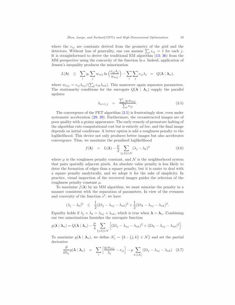
The convergence of the PET algorithm (3.5) is frustratingly slow, even undersystematic acceleration (29; 39). Furthermore, the reconstructed images are ofpoor quality with a grainy appearance. The early remedy of premature halting ofthe algorithm cuts computational cost but is entirely ad hoc, and the final imagedepends on initial conditions. A better option is add a roughness penalty to theloglikelihood. This device not only produces better images but also acceleratesconvergence. Thus, we maximize the penalized loglikelihood

f(λ) = L(λ) −µ

2

∑

{j,k}∈N

(λj − λk)2 (3.6)

where µ is the roughness penalty constant, and N is the neighborhood systemthat pairs spatially adjacent pixels. An absolute value penalty is less likely todeter the formation of edges than a square penalty, but it is easier to deal witha square penalty analytically, and we adopt it for the sake of simplicity. Inpractice, visual inspection of the recovered images guides the selection of theroughness penalty constant µ.

To maximize f(λ) by an MM algorithm, we must minorize the penalty in amanner consistent with the separation of parameters. In view of the evennessand convexity of the function s2, we have

(λj − λk)2 ≤1

2(2λj − λnj − λnk)2 +

1

2(2λk − λnj − λnk)2.

Equality holds if λj + λk = λnj + λnk, which is true when λ = λn. Combiningour two minorizations furnishes the surrogate function

g(λ | λn) = Q(λ | λn) −µ

4

∑

{j,k}∈N

[

(2λj − λnj − λnk)2 + (2λk − λnj − λnk)2]

.

To maximize g(λ | λn), we define Nj = {k : {j, k} ∈ N} and set the partialderivative

∂

∂λj

g(λ | λn) =∑

i

[yiwnij

λj

− eij

]

− µ∑

k:∈Nj

(2λj − λnj − λnk) (3.7)


equal to 0 and solve for λn+1,j . Multiplying equation (3.7) by λj produces aquadratic with roots of opposite signs. We take the positive root

λn+1,j =−bnj −

√

b2nj − 4ajcnj

2aj

,

where

aj = −2µ∑

k∈Nj

1, bnj =∑

k∈Nj

(λnj + λnk) − 1, cnj =∑

i

yiwnij .

Algorithm 2 summarizes the complete MM scheme. Obviously, complete param-eter separation is crucial. The quantities aj can be computed once and stored.The quantities bnj and cnj are computed for each j in parallel. To improveGPU performance in computing the sums over i, we exploit the widely availableparallel sum-reduction techniques (30). Given these results, a specialized butsimple GPU code computes the updates λn+1,j for each j in parallel.

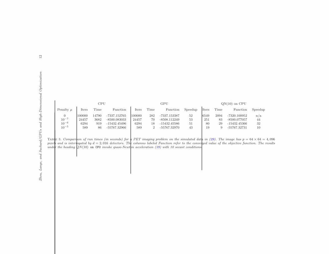
Table 3 compares the run times of the CPU and GPU implementations fora simulated PET image (29). The image as depicted in the top of Figure 3 hasp = 64 × 64 = 4, 096 pixels and is interrogated by d = 2, 016 detectors. Overallwe see a 43- to 53-fold reduction in run times with the GPU implementation.Figure 3 displays the true image and the estimated images under penalties ofµ = 0, 10−5, 10−6, and 10−7. Without penalty (µ = 0), the algorithm fails toconverge in 100,000 iterations.

Algorithm 2 (PET Image Recovering) Given the coefficient matrix E ∈ Rd×p+ ,

coincident counts y = (y1, . . . , yd) ∈ Zd+, and roughness parameter µ > 0,

find the intensity vector λ = (λ1, . . . , λp) ∈ Rp+ that maximizes the objective

function (3.6).Scale E to have unit l1 column norms.Compute |Nj | =

∑

k:{j,k}∈N1 and aj − 2µ|Nj | for all 1 ≤ j ≤ p.

Initialize: λ0j ← 1, j = 1, . . . , p.repeat

znij ← (yieijλnj)/(∑

keikλnk) for all 1 ≤ i ≤ d, 1 ≤ j ≤ p

for j = 1 to p do

bnj ← µ(|Nj |λnj +∑

k∈Njλnk)− 1

cnj ←∑

iznij

λn+1,j ← (−bnj −√

b2nj− 4ajcnj)/(2aj )

end for

until convergence occurs

3.3. Multidimensional Scaling

Multidimensional scaling (MDS) was the first statistical application of theMM principle (6; 5). MDS represents q objects as faithfully as possible in p-dimensional space given a nonnegative weight wij and a nonnegative dissimi-larity measure yij for each pair of objects i and j. If θ

i ∈ Rp is the position

Zhou,Lange

,and

Such

ard

/G

PU

sand

Hig

h-D

imen

sionalO

ptim

ization

12

CPU GPU QN(10) on CPU

Penalty µ Iters Time Function Iters Time Function Speedup Iters Time Function Speedup

0 100000 14790 -7337.152765 100000 282 -7337.153387 52 6549 2094 -7320.100952 n/a10−7 24457 3682 -8500.083033 24457 70 -8508.112249 53 251 83 -8500.077057 4410−6 6294 919 -15432.45496 6294 18 -15432.45586 51 80 29 -15432.45366 3210−5 589 86 -55767.32966 589 2 -55767.32970 43 19 9 -55767.32731 10

Table 3. Comparison of run times (in seconds) for a PET imaging problem on the simulated data in (29). The image has p = 64 × 64 = 4, 096pixels and is interrogated by d = 2, 016 detectors. The columns labeled Function refer to the converged value of the objective function. The resultsunder the heading QN(10) on CPU invoke quasi-Newton acceleration (39) with 10 secant conditions.


10 20 30 40 50 60

10

20

30

40

50

60

10 20 30 40 50 60

10

20

30

40

50

60

10 20 30 40 50 60

10

20

30

40

50

60

10 20 30 40 50 60

10

20

30

40

50

60

10 20 30 40 50 60

10

20

30

40

50

60

Fig 3. The true PET image (top) and the recovered images with penalties µ = 0, 10−7, 10−6,and 10−5.


of object i, then the p × q parameter matrix θ = (θ1, . . . , θq) is estimated byminimizing the stress function

f(θ) =∑

1≤i<j≤q

wij(yij − ‖θi − θj‖)2 (3.8)

=∑

i<j

wijy2ij − 2

∑

i<j

wijyij‖θi − θ

j‖ +∑

i<j

wij‖θi − θ

j‖2,

where ‖θi − θj‖ is the Euclidean distance between θ

i and θj . The stress func-

tion (3.8) is invariant under translations, rotations, and reflections of Rp. To

avoid translational and rotational ambiguities, we take θ1 to be the origin and

the first p−1 coordinates of θ2 to be 0. Switching the sign of θ2

p leaves the stressfunction invariant. Hence, convergence to one member of a pair of reflected min-ima immediately determines the other member.

Given these preliminaries, we now review the derivation of the MM algorithmpresented in (16). Because we want to minimize the stress, we majorize it. Themiddle term in the stress (3.8) is majorized by the Cauchy-Schwartz inequality

−‖θi − θj‖ ≤ −

(θi − θj)t(θi

n − θjn)

‖θin − θ

jn‖

.

To separate the parameters in the summands of the third term of the stress,we invoke the convexity of the Euclidean norm ‖ · ‖ and the square function s2.These maneuvers yield

‖θi − θj‖2 =

∥

∥

∥

1

2

[

2θi − (θi

n + θjn)

]

−1

2

[

2θj − (θj

n + θjn)

]∥

∥

∥

2

≤ 2∥

∥

∥θ

i −1

2(θi

n + θjn)

∥

∥

∥

2

+ 2∥

∥

∥θ

j −1

2(θi

n + θjn)

∥

∥

∥

2

.

Assuming that wij = wji and yij = yji, the surrogate function therefore becomes

g(θ | θn) = 2∑

i<j

wij

[

∥

∥

∥θ

i −1

2(θi

n + θjn)

∥

∥

∥

2

−yij(θ

i)t(θin − θ

jn)

‖θin − θ

jn‖

]

+2∑

i<j

wij

[

∥

∥

∥θ

j −1

2(θi

n + θjn)

∥

∥

∥

2

+yij(θ

j)t(θin − θ

jn)

‖θin − θ

jn‖

]

= 2

q∑

i=1

∑

j 6=i

[

wij

∥

∥

∥θ

i −1

2(θi

n + θjn)

∥

∥

∥

2

−wijyij(θ

i)t(θin − θ

jn)

‖θin − θ

jn‖

]

up to an irrelevant constant. Setting the gradient of the surrogate equal to the0 vector produces the parallel updates

θin+1,k =

∑

j 6=i

[

wijyij(θink−θ

j

nk)

‖θin−θ

jn‖

+ wij(θink + θj

nk)]

2∑

j 6=i wij


for all movable parameters θik.

Algorithm 3 summarizes the parallel organization of the steps. Again thematrix multiplications Θt

nΘn and Θn(W − Zn) can be taken care of by theCUBLAS library (25). The remaining steps of the algorithm are conducted byeasily written parallel code.

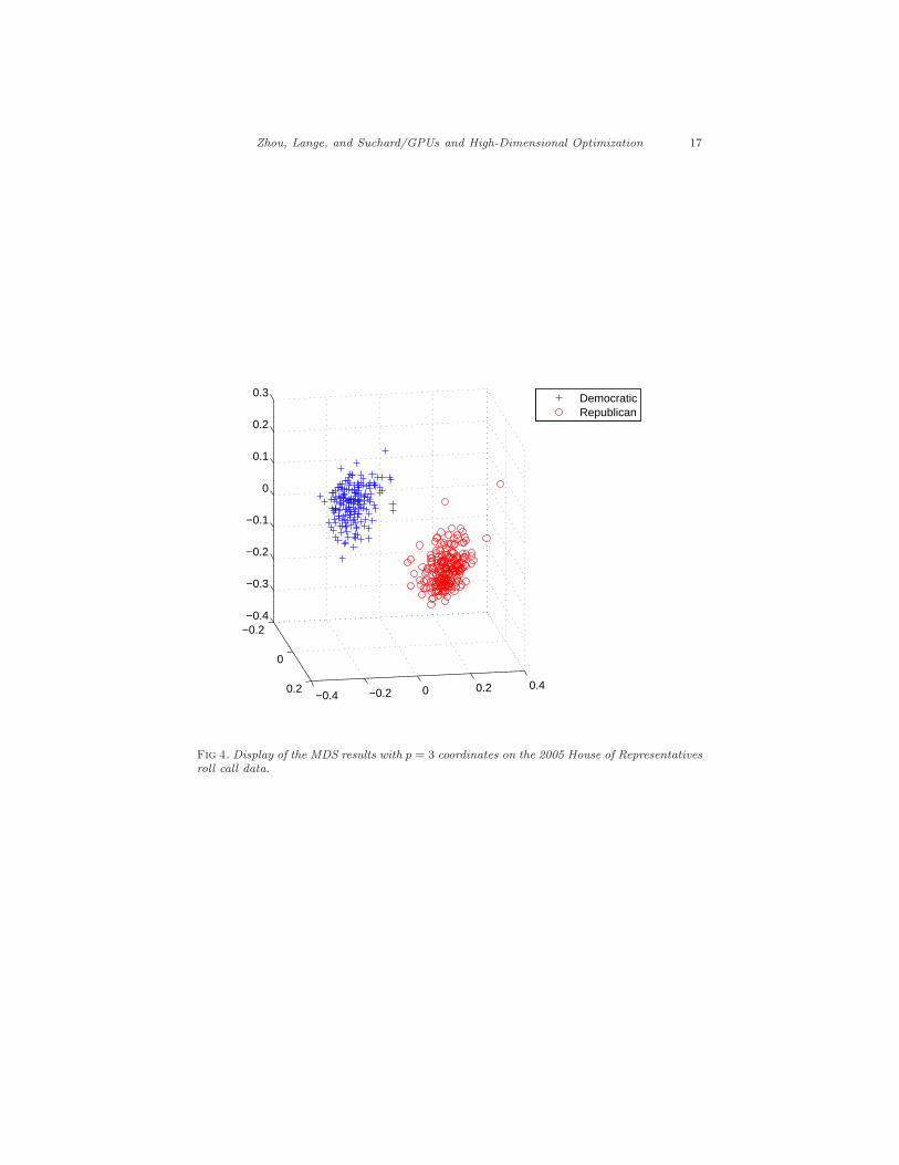
Table 4 compares the run times in seconds for MDS on the 2005 UnitedStates House of Representatives roll call votes. The original data consist of the671 roll calls made by 401 representatives. We refer readers to the reference (8)for a careful description of the data and how the MDS input 401× 401 distancematrix is derived. The weights wij are taken to be 1. In our notation, thenumber of objects (House Representatives) is q = 401. Even for this relativelysmall dataset, we see a 27–48 fold reduction in total run times, depending on theprojection dimension p. Figure 4 displays the results in p = 3 dimensional space.The Democratic and Republican members are clearly separated. For p = 30, thealgorithm fails to converge within 100,000 iterations.

Although the projection of points into p > 3 dimensional spaces may soundartificial, there are situations where this is standard practice. First, MDS is fore-most a dimension reduction tool, and it is desirable to keep p > 3 to maximizeexplanatory power. Second, the stress function tends to have multiple local min-ima in low dimensions (9). A standard optimization algorithm like MM is onlyguaranteed to converge to a local minima of the stress function. As the numberof dimensions increases, most of the inferior modes disappear. One can formallydemonstrate that the stress has a unique minimum when p = q − 1 (4; 9). Inpractice, uniqueness can set in well before p reaches q − 1. In the recent work(38), we propose a “dimension crunching” technique that increases the chanceof the MM algorithm converging to the global minimum of the stress function.In dimension crunching, we start optimizing the stress in a Euclidean space R

m

with m > p. The last m − p components of each column θi are gradually sub-

jected to stiffer and stiffer penalties. In the limit as the penalty tuning parametertends to ∞, we recover the global minimum of the stress in R

p. This strategyinevitably incurs a computational burden when m is large, but the MM+GPUcombination comes to the rescue.

Algorithm 3 (MDS) Given weights W and distances Y ∈ Rq×q, find the matrix

Θ = [θ1, . . . , θq] ∈ Rp×q which minimizes the stress (3.8).

Precompute: xij ← wijyij for all 1 ≤ i, j ≤ qPrecompute: wi· ←

∑

jwij for all 1 ≤ i ≤ q

Initialize: Draw θi0k

uniformly on [-1,1] for all 1 ≤ i ≤ q, 1 ≤ k ≤ prepeat

Compute ΘtnΘn

dnij ← {ΘtnΘn}ii + {Θt

nΘn}jj − 2{ΘtnΘn}ij for all 1 ≤ i, j ≤ q

znij ← xij/dnij for all 1 ≤ i 6= j ≤ qzni· ←

∑

jznij for all 1 ≤ i ≤ q

Compute Θn(W − Zn)θin+1,k

← [θink

(wi· + zni·) + {Θn(W − Zn)}ik ]/(2wi·) for all 1 ≤ i ≤ p, 1 ≤ k ≤ q

until convergence occurs

Zhou,Lange

,and

Such

ard

/G

PU

sand

Hig

h-D

imen

sionalO

ptim

ization

16

CPU GPU QN(20) on CPU

Dim-p Iters Time Stress Iters Time Stress Speedup Iters Time Stress Speedup

2 3452 43 198.5109307 3452 1 198.5109309 43 530 16 198.5815072 33 15912 189 95.55987770 15912 6 95.55987813 32 1124 38 92.82984196 54 15965 189 56.83482075 15965 7 56.83482083 27 596 18 56.83478026 115 24604 328 39.41268434 24604 10 39.41268444 33 546 17 39.41493536 1910 29643 441 14.16083986 29643 13 14.16083992 34 848 35 14.16077368 1320 67130 1288 6.464623901 67130 32 6.464624064 40 810 43 6.464526731 3030 100000 2456 4.839570118 100000 51 4.839570322 48 844 54 4.839140671 n/a

Table 4. Comparison of run times (in seconds) for MDS on the 2005 House of Representatives roll call data. The number of points (representatives)is q = 401. The results under the heading QN(20) on CPU invoke the quasi-Newton acceleration (39) with 20 secant conditions.


−0.2

0

0.2−0.4 −0.2 0 0.2 0.4

−0.4

−0.3

−0.2

−0.1

0

0.1

0.2

0.3

DemocraticRepublican

Fig 4. Display of the MDS results with p = 3 coordinates on the 2005 House of Representativesroll call data.


4. Discussion

The rapid and sustained increases in computing power over the last half cen-tury have transformed statistics. Every advance has encouraged statisticians toattack harder and more sophisticated problems. We tend to take the steadymarch of computational efficiency for granted, but there are limits to a chip’sclock speed, power consumption, and logical complexity. Parallel processing viaGPUs is the technological innovation that will power ambitious statistical com-puting in the coming decade. Once the limits of parallel processing are reached,we may see quantum computers take off. In the meantime statisticians shouldlearn how to harness GPUs productively.

We have argued by example that high-dimensional optimization is driven byparameter and data separation. It takes both to exploit the parallel capabilitiesof GPUs. Block relaxation and the MM algorithm often generate ideal parallelalgorithms. In our opinion the MM algorithm is the more versatile of the twogeneric strategies. Unfortunately, block relaxation does not accommodate con-straints well and may generate sequential rather than parallel updates. Evenwhen its updates are parallel, they may not be data separated. The EM algo-rithm is one of the most versatile tools in the statistician’s toolbox. The MMprinciple generalizes the EM algorithm and shares its positive features. Scoringand Newton’s methods become impractical in high dimensions. Despite thesearguments in favor of MM algorithms, one should always keep in mind hybridalgorithms such as the one we implemented for NNMF.

Although none of our data sets is really large by today’s standards, they dodemonstrate that a good GPU implementation can easily achieve one to twoorders of magnitude improvement over a single CPU core. Admittedly, modernCPUs come with 2 to 8 cores, and distributed computing over CPU-based clus-ters remains an option. But this alternative also carries a hefty price tag. TheNVIDIA GTX280 GPU on which our examples were run drives 240 cores at acost of several hundred dollars. High-end computers with 8 or more CPU nodescost thousands of dollars. It would take 30 CPUs with 8 cores each to equal asingle GPU at the same clock rate. Hence, GPU cards strike an effective andcost efficient balance.

The simplicity of MM algorithms often comes at a price of slow (at best lin-ear) convergence. Our MDS, NNMF, and PET (without penalty) examples arecases in point. Slow convergence is a concern as statisticians head into an eradominated by large data sets and high-dimensional models. Think about thescale of the Netflix data matrix. The speed of any iterative algorithm is deter-mined by both the computational cost per iteration and the number of iterationsuntil convergence. GPU implementation reduces the first cost. Computationalstatisticians also have a bag of software tricks to decrease the number of itera-tions (22; 10; 20; 14; 11; 23; 35). For instance, the recent paper (39) proposesa quasi-Newton acceleration scheme particularly suitable for high-dimensionalproblems. The scheme is off-the-shelf and broadly applies to any search algo-rithm defined by a smooth algorithm map. The acceleration requires only mod-est increments in storage and computation per iteration. Tables 3 and 4 also


list the results of this quasi-Newton acceleration of the CPU implementationfor the MDS and PET examples. As the tables make evident, quasi-Newtonacceleration significantly reduces the number of iterations until convergence.The accelerated algorithm always locates a better mode while cutting run timescompared to the unaccelerated algorithm. We have tried the quasi-Newton ac-celeration on our GPU hardware with mixed results. We suspect that the lackof full double precision on the GPU is the culprit. When full double precisionbecomes widely available, the combination of GPU hardware acceleration andalgorithmic software acceleration will be extremely potent.

Successful acceleration methods will also facilitate attacking another nag-ging problem in computational statistics, namely multimodality. No one knowshow often statistical inference is fatally flawed because a standard optimizationalgorithm converges to an inferior mode. The current remedy of choice is tostart a search algorithm from multiple random points. Algorithm accelerationis welcome because the number of starting points can be enlarged without anincrease in computing time. As an alternative to multiple starting points, ourrecent paper (38) suggests modifications of several standard MM algorithmsthat increase the chance of locating better modes. These simple modificationsall involve variations on deterministic annealing (34).

Our treatment of simple classical examples should not hide the wide appli-cability of the powerful MM+GPU combination. A few other candidate ap-plications include penalized estimation of haplotype frequencies in genetics (1),construction of biological and social networks under a random multigraph model(28), and data mining with a variety of models related to the multinomial dis-tribution (40). Many mixture models will benefit as well from parallelization,particularly in assigning group memberships. Finally, parallelization is hardlylimited to optimization. We can expect to see many more GPU applications inMCMC sampling. Given the computationally intensive nature of MCMC, theultimate payoff may even be higher in the Bayesian setting than in the frequen-tist setting. Of course realistically, these future triumphs will require a greatdeal of thought, effort, and education. There is usually a desert to wander anda river to cross before one reaches the promised land.

Acknowledgements

M.S. acknowledges support from NIH grant R01 GM086887. K.L. was supportedby United States Public Health Service grants GM53275 and MH59490.

References

[1] Ayers, K. L. and Lange, K. L (2008). Penalized estimation of haplotypefrequencies. Bioinformatics 24 1596–1602.

[2] Berry, M. W., Browne, M., Langville, A. N., Pauca, V. P., andPlemmons, R. J. (2007). Algorithms and applications for approximate


nonnegative matrix factorization. Comput. Statist. Data Anal. 52 155–173.MR2409971

[3] Buckner, J., Wilson J., Seligman, M., Athey, B., Watson, S. andMeng, F. (2009) The gputools package enables GPU computing in R. Bioin-formatics 22 btp608.

[4] de Leeuw, J. Fitting distances by least squares. unpublished manuscript.[5] de Leeuw, J. and Heiser, W. J. (1977). Convergence of correction ma-

trix algorithms for multidimensional scaling. Geometric Representations ofRelational Data, 133–145. Mathesis Press, Ann Arbor, MI.

[6] de Leeuw, J. (1977). Applications of convex analysis to multidimensionalscaling. Recent developments in statistics (Proc. European Meeting Statisti-cians, Grenoble, 1976), 133–145. North-Holland, Amsterdam.

[7] Dempster, A. P., Laird, N. M., and Rubin, D. B. (1977). Maximumlikelihood from incomplete data via the EM algorithm. (with discussion) J.Roy. Statist. Soc. Ser. B 39 1–38. MR0501537

[8] Diaconis, P., Goel, S., and Holmes, S. (2008). Horseshoes in multidi-mensional scaling and local kernel methods. Annals of Applied Statistics 2

777–807.[9] Groenen, P. J. F. and Heiser, W. J. (1996). The tunneling method for

global optimization in multidimensional scaling. Pshychometrika 61 529–550.[10] Jamshidian, M. and Jennrich, R. I. (1993). Conjugate gradient acceler-

ation of the EM algorithm. J. Amer. Statist. Assoc. 88 221–228. MR1212487[11] Jamshidian, M and Jennrich, R. I. (1997). Acceleration of the EM al-

gorithm by using quasi-Newton methods. J. Roy. Statist. Soc. Ser. B 59

569–587. MR1452026[12] Koren, Y, Bell, R., and Volinsky, C. (2009). Matrix factorization

techniques for recommender systems. Computer 42 30–37.[13] Lange, K. L. and Carson, R. (1984). EM reconstruction algorithms for

emission and transmission tomography. J. Comput. Assist. Tomogr. 8 306–316.

[14] Lange, K. L. (1995). A quasi-Newton acceleration of the EM algorithm.Statist. Sinica 5 1–18. MR1329286

[15] Lange, K. L. (2004). Optimization. Springer-Verlag, New York.MR2072899

[16] Lange, K. L., Hunter, D. R., and Yang, I. (2000). Optimization trans-fer using surrogate objective functions. (with discussion) J. Comput. Graph.Statist. 9 1–59. MR1819865

[17] Lee, A., Yan, C., Giles, M. B., Doucet, A., and Holmes, C. C.

(2009). On the utility of graphics cards to perform massively parallel sim-ulation of advanced Monte Carlo methods. Technical report, Department ofStatistics, Oxford University.

[18] Lee, D. D. and Seung, H. S. (1999). Learning the parts of objects bynon-negative matrix factorization. Nature 401 788–791.

[19] Lee, D. D. and Seung, H. S. (2001). Algorithms for non-negative matrixfactorization. NIPS, pages 556–562, MIT Press.

[20] Liu, C. and Rubin, D. B. (1994). The ECME algorithm: a simple ex-

http://www.ams.org/mathscinet-getitem?mr=2409971








tension of EM and ECM with faster monotone convergence. Biometrika 81

633–648. MR1326414[21] McLachlan, G. J. and Krishnan, T. (2008). The EM algorithm and

extensions. Wiley-Interscience [John Wiley & Sons], Hoboken, NJ, secondedition. MR2392878

[22] Meng, X. L. and Rubin, D. B. (1993). Maximum likelihood estima-tion via the ECM algorithm: a general framework. Biometrika 80 267–278.MR1243503

[23] Meng, X. L. and van Dyk, D. (1997). The EM algorithm—an old folk-song sung to a fast new tune. (with discussion) J. Roy. Statist. Soc. Ser. B,59(3):511–567. MR1452025

[24] MIT center for biological and computational learning. CBCL Face Database#1, http://www.ai.mit.edu/projects/cbcd.

[25] NVIDIA (2008). NVIDIA CUBLAS Library.[26] NVIDIA (2008). NVIDIA CUDA Compute Unified Device Architecture:

Programming Guide Version 2.0.[27] Owens, J. D., Luebke, D., Govindaraju, N., Harris, M., Kruger,

J., Lefohn, A. E., and Purcell, T. J. (2007). A survey of general-purposecomputation on graphics hardware. Computer Graphics Forum 26 80–113.

[28] Ranola, J.M., Ahn, S., Sehl, M.E., Smith, D.J. and Lange, K. L.

(2010) A Poisson model for random multigraphs. unpublished manuscript.[29] Roland, C., Varadhan, R., and Frangakis, C. E. (2007). Squared

polynomial extrapolation methods with cycling: an application to the positronemission tomography problem. Numer. Algorithms 44 159–172. MR2334694

[30] Silberstein, M., Schuster, A., Geiger, D., Patney, A., and Owens,

J. D. (2008). Efficient computation of sum-products on GPUs throughsoftware-managed cache. Proceedings of the 22nd Annual International Con-ference on Supercomputing, pages 309–318, ACM.

[31] Sinnott-Armstrong, N. A., Greene, C. S., Cancare, F., andMoore, J. H. (2009). Accelerating epistasis analysis in human genetics withconsumer graphics hardware. BMC Research Notes 2 149.

[32] Suchard, M. A. and Rambaut, A. (2009). Many-core algorithms forstatistical phylogenetics. Bioinformatics 25 1370–1376.

[33] Tibbits, M. M., Haran, M., and Liechty, J. C. (2009). Parallel multi-variate slice sampling. Statistics and Computing, to appear.

[34] Ueda, N. and Nakano, R. (1998). Deterministic annealing EM algorithm.Neural Networks 11 271 – 282.

[35] Varadhan, R. and Roland, C. (2008). Simple and globally convergentmethods for accelerating the convergence of any EM algorithm. Scand. J.Statist. 35 335–353. MR2418745

[36] Vardi, Y., Shepp, L. A., and Kaufman, L. (1985). A statistical modelfor positron emission tomography. (with discussion) J. Amer. Statist. Assoc.80 8–37. MR786595

[37] Wu, T. T. and Lange, K. L. (2009). The MM alternative to EM. Stat.Sci., in press.

[38] Zhou, H. and Lange K. L. (2009). On the bumpy road to the dominant





http://www.ai.mit.edu/projects/cbcd





mode. Scandinavian Journal of Statistics, in press.[39] Zhou, H., Alexander, D., and Lange, K. L. (2009). A quasi-newton ac-

celeration for high-dimensional optimization algorithms. Statistics and Com-puting, DOI:10.1007/s11222-009-9166-3.

[40] Zhou, H. and Lange, K. L. (2009). MM algorithms for some discretemultivariate distributions. J Computational Graphical Stat, in press.

graphics processing units and high-dimensional optimization · graphics processing units and...

Documents