Graphical Models for Game TheoryGraphical Models for Game Theory

by

Michael Kearns,

Michael L. Littman,

Satinder Singh

Presented by: Gedon Rosner

AgendaAgenda• Introduction

• Motivation• Goals

• Terminology• The Algorithm

• Outline• Details• Proof

• Back up

IntroductionIntroduction

• This paper describes a graphical representation of multi-player single-stage games.

• Presents a polynomial algorithm that provides approximations to well-defined problems that would otherwise be computationally hard.

• Presents an exponential algorithm with precise results that will not be described.

Introduction – cont.Introduction – cont.• Multi-Player game theory uses Tables to

represent games – payoffs to each player per their course of action.

• Tables require immense computational resources (space & time).

• In certain cases graphical structures succinctly describe the game and may be computationally less expensive as well (depending on what is computed).

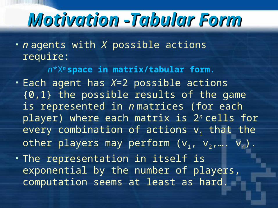
Motivation -Tabular FormMotivation -Tabular Form• n agents with X possible actions require:

n*Xn space in matrix/tabular form.

• Each agent has X=2 possible actions {0,1} the possible results of the game is represented in n matrices (for each player) where each matrix is 2n cells for every combination of actions vi that the other players may perform (v1, v2,…. vn).

• The representation in itself is exponential by the number of players, computation seems at least as hard.

Motivation-Graphical FormMotivation-Graphical Form

• Matrices ~ Graphs :- special graphs (e.g. trees) are better used to describe sparse Matrices.

• A full graph (V,E) is isomorphic to a matrix. • Trees - graph traversal algorithms are “better”

for flowflow computation – representing dependencies.

• If a game has dependencies between sets of localized players and mutual influence is propagated “across the board” a tree structure is inherent.

Motivation - ComputationMotivation - Computation

• Nash Equilibriums are sets of strategies in which no player can unilaterally change his/her strategy and gain benefit (=local maxim).

• Radio stations music vs. rating benefit:

A\BמזרחיתMTVישראלית

50,20 50,30 25,25מזרחית

MTV30,50 15,15 30,20

10,10 20,30 20,50ישראלית

Nash equilibriumNash equilibrium

• The danger is that both stations will choose the more profitable מזרחית format -- and split the market, getting only 25 each! Actually, there is an even worse danger that each station might assume that the other station will choose and each choose MTV, splitting that ,מזרחיתmarket and leaving each with a market share of just 15.

GoalsGoals

1. Provide a complete graphical representation for multi-player one-stage games.

2. Define how/when the graphical structure may provide a succinct representation in an order of magnitude. (polynomial vs. exponential).

3. Provide a polynomial algorithm for computing approximate Nash equilibriums in one stage games by trees or sparse graphs.

AgendaAgenda• Introduction

• Motivation• Goals

• Terminology• The Algorithm

• Outline• Details• Proof

• Back up

TerminologyTerminology

• Games in Tabular form:

An n-player, two-action game is defined by n matrices Mi with n indices. The entry Mi(x1,.. xn) specifies the payoff to player i when the combined action of the n players is x {0,1}n.

Each matrix has 2n entries.• Pure and Mixed Strategies:

The actions of either 0 or 1 are pure. A mixed strategy is a probability pi the player will play 0.

Terminology – cont.Terminology – cont.

• Expected Payoff for mixed strategy:

Player i expects the payoff Mi(p) which is defined as the Exp.x~p[Mi(p)].

here x~p indicates that:

xj = 0 pj.

xj = 1 1- pj.

• Nash Theorem (1951):

For any game, there exists a Nash equilibrium in the space of joint mixed strategies.

{

Terminology – cont. Terminology – cont.

• Nash equilibrium:

A mixed strategy of all the players denoted as.

p s.t. for any player i and for any other strategy p[0,1]: Mi(p) Mi(p[i:pi]). This just means that no player can improve their payoff by deviating unilaterally from the Nash equilibrium.

-Nash equilibrium:

Mi(p)+ Mi(p[i:pi]) – improve by at most .

AgendaAgenda• Introduction

• Motivation• Goals

• Terminology• The Algorithm

• Outline• Details• Proof

• Back up

Graphical Game description Graphical Game description

• An n-player game is - (G,M): G is an undirected graph on n vertices and Mi is a set of n matrices for each player. Player i is represented by a vertex labeled i.

• NG(i){1,…,n} – the neighbors j of i in G s.t. the undirected edge (i,j)E(G) and (i,i) NG(i).

• If | NG(i)|k then p [0,1]k the expected payoff is effected by k neighbors only and Mi(p) = Exp.x~p[Mi(p)] = O(2k) << O(2k).

?

A Complete DescriptionA Complete Description

• Proof:There is a complete mapping between graph representation and tabular representation. Every game has a trivial representation as a graphical game by choosing the complete graph.

In cases (like Bayesian networks) where a flow or a local neighborhood may be defined and can be bound by k << n, exponential space saving occurs.

Attaining Goal #1 + #2

The Tree Algorithm - AbstractThe Tree Algorithm - Abstract

• The graphical game is (G,M). G is a tree.• The computation is an -Nash equilibrium of

the game.• The algorithm traverses the tree in reverse

depth-first order using a relaxation computation in each step. Inductively a group of Nash equilibrium is determined.

• Finally the tree is traversed in depth-first ordering where a single Nash equilibrium is chosen.

Terminology of the gameTerminology of the game

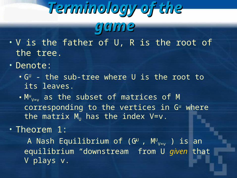
• V is the father of U, R is the root of the tree.• Denote:

• GU - the sub-tree where U is the root to its leaves.

• MuV=v as the subset of matrices of M corresponding

to the vertices in Gu where the matrix MU has the index V=v.

• Theorem 1: A Nash Equilibrium of (GU , MU

V=v ) is an equilibrium “downstream” from U given that V plays v.

Traversing the TreeTraversing the Tree

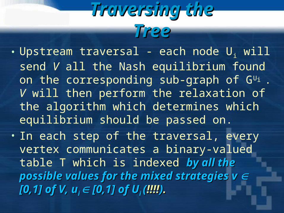
• Upstream traversal - each node Ui will send V all the Nash equilibrium found on the corresponding sub-graph of GUi . V will then perform the relaxation of the algorithm which determines which equilibrium should be passed on.

• In each step of the traversal, every vertex communicates a binary-valued table T which is indexed by all the possible values for the mixed by all the possible values for the mixed strategies v strategies v [0,1] of V, u [0,1] of V, ui i [0,1] of U [0,1] of Ui i ((!!!!!!!!))..

The RelaxationThe Relaxation

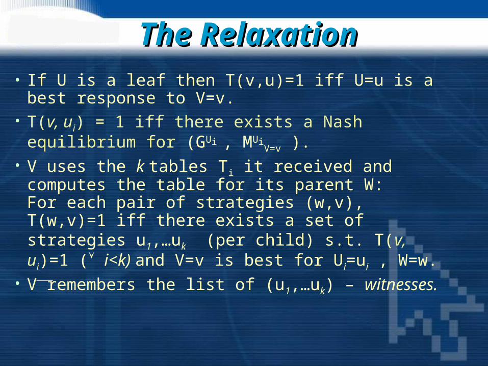
• If U is a leaf then T(v,u)=1 iff U=u is a best response to V=v.

• T(v, ui) = 1 iff there exists a Nash equilibrium for (GUi , MUi

V=v ).• V uses the k tables Ti it received and computes

the table for its parent W: For each pair of strategies (w,v), T(w,v)=1 iff there exists a set of strategies u1,…uk (per child) s.t. T(v, ui)=1 ( i<k) and V=v is best for Ui=ui , W=w.

• V remembers the list of (u1,…uk) – witnesses.

Abstract Algorithm ProofAbstract Algorithm Proof

Base case: Every leaf U sends its parent V the table T(v,u)

for every strategy pair (v,u).General case: If T(w,v)=1 for some pair (w,v) then there exists

a witness (u1,…uk) s.t. T(v, ui)=1 for all i. Induction assumption & Theorem 1 there exists

a downstream equilibrium s.t. each Ui=ui ; since V=v is the best response - the equilibrium is from V.

Abstract Algorithm Proof – Abstract Algorithm Proof – cont.cont.

• If T(w,v)=0 using the same reasoning there is no equilibrium in which W=w and V=v.

• Nash Theorem concludes and assures that for every game there exists at least one pair (w,v) s.t. T(w,v) = 1.

• R receives a table that along with the witnesses represent all Nash equilibriums.

• R chooses a strategy non-deterministically and informs its sons – one of the strategies is determined at the end of the downstream flow.

AgendaAgenda• Introduction

• Motivation• Goals

• Terminology• The Algorithm

• Outline• Details• Proof

• Back up

Details…Details …Details…Details …

• Claimed to find an approximation of a Nash equilibrium in O(n) – looks like we’ve found every Nash equilibrium ??

• The table T(w,v) is unrealistic – w,v are continues not discrete.

• There may be exponential numbers of Nash Equilibrium – a deterministic algorithm can’t be polynomial.

Quantification Quantification

• Instead of continues values – discrete values with finite size and computational ease.

• Determine a grid {0,,2 ,…,1}. Player i plays qi {0,,2 ,…,1} and q {0,,2 ,…,1}n.

• Each table consists of binary values for 1/ 2 entries.

• Finding best responses is a simple search across the table and are now approximate best responses.

AgendaAgenda• Introduction

• Motivation• Goals

• Terminology• The Algorithm

• Outline• Details• Proof

• Back up

Determining Determining

1. needs to insure that the loss suffered by any player in moving to the grid is bound.

2. needs to insure the Nash equilibriums may be approximately preserved existence of an –Nash equilibrium.

3. needs to be scalable to the size of the representation to allow the algorithm to be polynomial – 1/ = O(nx).

Bound Loss of Players - #1Bound Loss of Players - #1

• Let | NG(i)|=k then as defined

Mi(p) = Exp.x~p[Mi(p)]

)()1()(}1,0{ 1

1 xMpp ix

k

j

xj

xj

k

jj

• Remember xj = {0,1} so this is merely the probability that x actually occurs.

Lemma 1Lemma 1

• Let p,q [0,1]k satisfy |pi – qi| (i=1..k).

Then provided 4/ (k log2(k/2)) :

τkkqpk

ii

k

ii

log11

• Proof by induction on k:

Base case k =2: k · logk = 2 2 ( p2+q2) |p1- q1|·( p2+q2) |p1 p2 - q1 q2| + |p1 q2 - q1 p2| |p1 p2 - q1 q2|

Lemma 1 – Proof cont.Lemma 1 – Proof cont.

• Without loss of generality assume k is even.

2

1

1)2/(

2/

11)2/(

2/

11

)))2/)(log(2/(()1(log

))2/(log()2/(

))2/(log()2/(

kkkkp

kkp

kkpqqq

k

ii

k

kii

k

ii

k

kii

k

ii

k

ii

• The lemma holds if -k+((k/2)(log(k/2)))2 0.

So 4/(k·log2(k/2)).

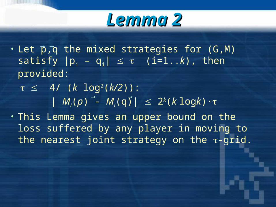
Lemma 2Lemma 2

• Let p,q the mixed strategies for (G,M) satisfy |pi – qi| (i=1..k), then provided:

4/ (k log2(k/2)):

| Mi(p) - Mi(q)| 2k(k logk)·

• This Lemma gives an upper bound on the loss suffered by any player in moving to the nearest joint strategy on the -grid.

Lemma 2 - ProofLemma 2 - Proof

)log(2

)log(

)()1()()1()(

)()1()()1()(

)()(

}1,0{

}1,0{ 1

1

1

1

}1,0{ 1

1

1

1

kk

kk

xMqqpp

xMqqpp

qMpM

k

x

ix

k

j

xj

xj

k

j

xj

xj

ix

k

j

xj

xj

k

j

xj

xj

ii

k

k

jjjj

k

jjjj

– –Nash equilibrium - #2Nash equilibrium - #2

Lemma 3: Let p be a Nash equilibrium for (G,M) and let q

be the nearest mixed strategy on the grid. Then provided 4/(k log2(k/2)): q is a 2k+1(k·log(k) · - Nash Equilibrium for (G,M).

Proof:

Let ri be the best response for player i to q. We bound Mi(q[i: ri]) - Mi(q) which is the benefit player i could attain from deviating from q.

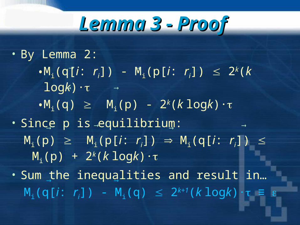
Lemma 3 - ProofLemma 3 - Proof

• By Lemma 2:

• Mi(q[i: ri]) - Mi(p[i: ri]) 2k(k logk)·

• Mi(q) Mi(p) - 2k(k logk)·• Since p is equilibrium:

Mi(p) Mi(p[i: ri]) Mi(q[i: ri]) Mi(p) + 2k(k logk)·

• Sum the inequalities and result in…

Mi(q[i: ri]) - Mi(q) 2k+1(k logk)· ≡

Polynomial scalabilityPolynomial scalability

• We now choose in accordance with the constraints: 2k+1(k logk)·

4/(k log2(k/2)) So:

min(/ 2k+1(k logk) , 4/(k log2(k/2)) ) Notice that is exponential to k << n. Each

step in the algorithm computes over (1/ )2 entries totaling (1/ )2k, the complete run time is polynomial in n.

Back up

Graphical Models for Game TheoryGraphical Models for Game Theory