velocity determination for pore pressure prediction · velocity determination for pore pressure...

28 CSEG RECORDER April 2006

Continued on Page 29

Velocity determination for pore pressure prediction Satinder Chopra* and Alan Huffman**

*Arcis Corporation, Calgary, Alberta, Canada; **Fusion Petroleum Technologies, Houston, USA

Summary

Knowledge of formation pore pressure is not only essentialfor safe and cost-effective drilling of wells, but is also criticalfor assessing exploration risk factors including the migrationof formation fluids and seal integrity. Usually, pre-drill esti-mates of pore pressure are derived from surface seismic databy first estimating seismic velocities and then utilizingvelocity-to-effective stress transforms appropriate for a givenarea combined with an estimated overburden stress to obtainpore pressure. So, the accuracy of velocity models used forpore pressure determination is of paramount importance.This paper briefly discusses some of the causes and mecha-nisms of overpre s s u res, and then reviews the availablemethods of velocity model building, mentioning therein theshortcomings and/or the advantages of each.

Introduction

An understanding of the rock/fluid characteristics of subsur-face formations is of critical importance in the evolution of oiland gas fields. During the exploration phase, pore pressureprediction for example helps in studying the hydrocarbontrap seals, mapping of hydrocarbon migration pathways,analyzing trap configurations and basin geometry andproviding calibrations for basin modeling. Predrill pore pres-sure prediction allows for appropriate mud weight to beselected and drill casing program to be optimised, therebyenabling safe and economic subsurface drilling. The impor-tance of determination of this information has gradually beenrealized as some major well disasters have led to the loss ofprecious human life, material and adverse publicity. It is timenow that pore pressure prediction formed an integral part ofprospect evaluation and well planning.

Besides drilling a well, the only way to predict potentialhazards like overpressured subsurface zones is through theuse of seismic surveys. Although such an analysis originatedwith the work of Terzaghi (1930) ( a soilscientist), it was the works of Hottman andJohnson (1965) (both petrophysicists) andPennebaker (1968) (drilling engineer), thatdrew the attention of geoscientists. While arange of disciplines are involved andneeded in a comprehensive pore pressureanalysis, geophysicists play a key role inmany ways (Bruce, 2002). Seismic methodsdetect changes of interval velocities withdepth from velocity analysis of CMP data,and so geophysicists are involved inseismic interpretation and determination ofrock properties which are related with porep re s s u re (Bell, 2002). Over pre s s u re dformations exhibit several of the followingproperties when compared with a normally

pressured section at the same depth (Dutta, 2002): (1) higherporosities (2) lower bulk densities (3) lower effective stresses(4) higher temperatures (5) lower interval velocities (6) higherPoisson’s ratios.

Seismic interval velocities get influenced by changes in eachof these properties and this is exhibited in terms of reflectionamplitudes in seismic surveys. Consequently, velocity deter-mination is the key to pore pressure prediction.

Some definitions

A detailed description of pore pressure terminology can be found in Bruce and Bowers (2002), Bowers (2002) and Dutta (2002). We include some of these definitions herefor convenience.

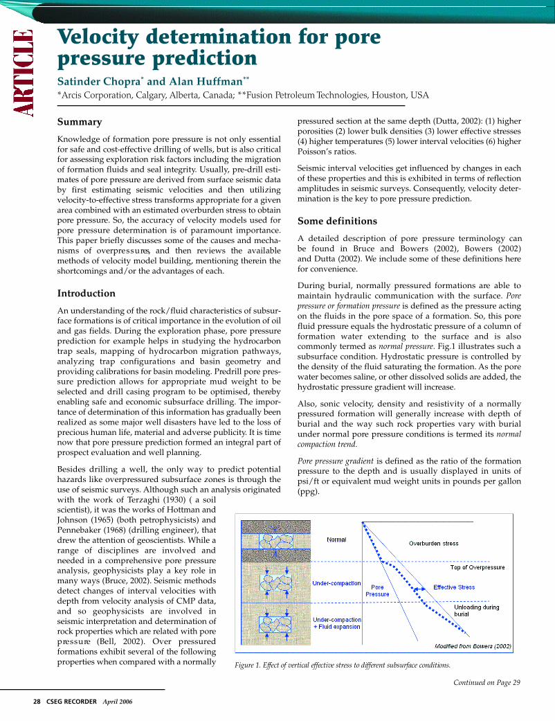
During burial, normally pressured formations are able tomaintain hydraulic communication with the surface. Porepressure or formation pressure is defined as the pressure actingon the fluids in the pore space of a formation. So, this porefluid pressure equals the hydrostatic pressure of a column offormation water extending to the surface and is alsocommonly termed as normal pressure. Fig.1 illustrates such asubsurface condition. Hydrostatic pressure is controlled bythe density of the fluid saturating the formation. As the porewater becomes saline, or other dissolved solids are added, thehydrostatic pressure gradient will increase.

Also, sonic velocity, density and resistivity of a normallypressured formation will generally increase with depth ofburial and the way such rock properties vary with burialunder normal pore pressure conditions is termed its normalcompaction trend.

Pore pressure gradient is defined as the ratio of the formationpressure to the depth and is usually displayed in units ofpsi/ft or equivalent mud weight units in pounds per gallon(ppg).

F i g u re 1. Effect of vertical effective stress to different subsurface conditions.

April 2006 CSEG RECORDER 29

Article Cont’d


Overburden pressure at any depth is the pressure that results fromthe combined weight of the rock matrix and the fluids in the porespace overlying the formation of interest. Overburden pressureincreases with depth and is also called the vertical stress.

Effective pressure is defined as the pressure acting on the solidrock framework. Terzaghi defined it as the difference betweenthe overburden pressure and the pore pressure.

Effective pre s s u re thus controls the compaction that takes place inp o rous granular media including sedimentary rocks and this hasbeen confirmed by laboratory studies (Tosaya, 1982; Dvorkin(1999)). Any process or condition causing a reduction of eff e c t i v es t ress will result in overpre s s u re. In overpre s s u res, the pore fluidsbear part of the weight of the overlying rocks. A lower eff e c t i v es t ress and a higher porosity tend to lower the rock velocity.C o n s e q u e n t l y, a relationship between velocity and effective stre s s ,p o rosity and lithology could be used to study pore pre s s u re s .

Causes of overpressure

Overpressures in sedimentary basins have been attributed todifferent mechanisms but the main ones are related to increase instress and in-situ fluid generating mechanisms. The ability ofeach of these processes to generate overpressures depends on therock and fluid properties of the sedimentary rocks and their rateof change under the normal range of basin conditions.

I n c rease in stre s s : During deposition of sediments, with thei n c rease in vertical stress, the pore fluids escape as the pore spacestry to compact. If a layer of low permeability, e.g. clay, pre v e n t sthe escape of pore fluids at rates sufficient to keep up with therate of increase in vertical stress, the pore fluid begins to carry al a rge part of the load and pore-fluid pre s s u re will increase. Thisp rocess is re f e r red to as u n d e rcompaction or compaction disequilib-r i u m (Hubbert and Rubey, 1959), and is by far the most wellunderstood overpre s s u re mechanism used to explain and quan-tify overpre s s u res in Tertiary basins where rapid deposition andsubsidence occur, e.g. the Mississippi, Ornico and Niger Deltaregions (Yassir and Addis, 2002).

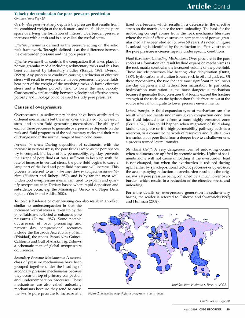
Tectonic subsidence or overthrusting can also result in an eff e c tsimilar to undercompaction in that thei n c reased vertical stress is taken up by thep o re fluids and reflected as enhanced porep re s s u res (Dutta, 1987). Some notableo c c u r rences of over pressuring andp resent day compressional tectonicsinclude the Barbados A c c retionary Prism( Trinidad), the Andes, Papua New Guinea,California and Gulf of Alaska. Fig. 2 showsa schematic map of global overpre s s u reo c c u r re n c e s .

Secondary Pressure Mechanisms: A secondclass of pressure mechanisms have beengrouped together under the heading ofsecondary pressure mechanisms becausethey occur on top of primary compactionand undercompaction processes. Thesemechanisms are also called unloadingmechanisms because they tend to causethe in-situ pore pressure to increase at a

fixed overburden, which results in a decrease in the effectivestress on the matrix, hence the term unloading. The basis for theunloading concept comes from the rock mechanics literaturewhere the role of effective stress on compaction of porous gran-ular media has been studied for over 50 years. As noted in figure1, unloading is identified by the reduction in effective stress asthe pore pressure increases rapidly under specific conditions.

Fluid Expansion Unloading Mechanisms: Over pre s s u re in the porespaces of a formation can result by fluid expansion mechanisms asthe rock matrix constrains the increased volume of the pore fluid.These include processes like heating, clay dehydration (Dutta,1987), hydrocarbon maturation (source rock to oil and gas), etc. Ofthese mechanisms, the two that are most significant in real ro c k sa re clay diagenesis and hydrocarbon maturation. In particular,h y d rocarbon maturation is the most dangerous mechanismbecause it generates fluid pre s s u res that locally exceed the fractures t rength of the rocks as the hydrocarbon fluids fracture out of thes o u rce interval to migrate to lower pre s s u re enviro n m e n t s .

Lateral transfer: A fluid-expansion type of mechanism can alsoresult when sediments under any given compaction conditionhas fluid injected into it from a more highly-pressured zone(Fertl, 1976). This could happen when migration of fluid alongfaults takes place or if a high-permeability pathway such as areservoir, or a connected network of reservoirs and faults allowstransmission of pore fluid from a deeper trap to a shallower one,a process termed lateral transfer.

Structural Uplift: A very dangerous form of unloading occurswhen sediments are uplifted by tectonic activity. Uplift of sedi-ments alone will not cause unloading if the overburden load is not changed, but when the overburden is reduced duringuplift either by syn-depositional tectonic processes or by erosion,the accompanying reduction in overburden results in the orig-inal in-s i t u p o re pre s s u re being contained by a much lower over-b u rden, which results in a reduction of the effective stress, andunloading.

For more details on overpressure generation in sedimentarybasins, the reader is referred to Osborne and Swarbrick (1997)and Huffman (2002).

Velocity determination for pore pressure prediction Continued from 8

F i g u re 2. Schematic map of global overpre s s u re occurre n c e s .


Article Cont’d

Continued on 1

Detection of Overpressures

The methods currently being used for detection of overpressuresexploit the deviation of formation properties from an expected ornormal trend in the area of interest. Well logs provide the mostextensively used and a reliable means to construct trends anddetect overpre s s u res. Usually, density, resistivity and sonicvelocity data either continue to increase or remain constant afterthey depart from their normal trends. However, this informationis forthcoming only after the well has been drilled. Detection ofoverpressures before drilling is more useful as precautions canbe taken and planning can be done accordingly. Reflectionseismic methods are commonly used for this purpose and exploitthe fact that overpressured intervals have lower velocities andimpedances that are lower than normally pressured intervals atthe same depth.

Empirical relationshipsAs porosity is a direct measure of compaction, Athy (1930) putforward the following exponential relationship between porosityand depth

ϕ(z) = ϕ0e−cz

where ϕ(z) is porosity at depth, ϕ0 is the porosity at z=0 and c isa constant.

Since then other modifications have been suggested to thismodel and this equation has been recast into (Dutta 2002),

ϕ(z) = ϕ0e−κσ

where coefficient k is related to the bulk density of the sedimentsand the density of pore water and σ is the effective stress.

Terzaghi’s equation is given as follows

ϕ(z) = 1 - ϕ0σc/4.606

and there are other empirical relationships as well.

One of these relationships is used to compute the effective stressfrom the porosity and then the pore pressure is computed easilyfrom Terzaghi’s relationship

S = P + σ

S = vertical overburden stress

P = pore fluid stress

σ= effective stress acting on the rock frame.

The commonly used approach for relating acoustic intervalvelocity to pore pressure is the Eaton’s empirical method (Eaton,1968, 1972).

According to Eaton

PP=Pobs – (Pobs – Phyd)x (ViVn)3

where

Pp = Predicted (shale) pore pressure

Pobs = Overburden pressure (rocks and fluids)

Phyd = Hydrostatic pressure (fluids)

Vi = Interval velocity (seismic data)

Vn = Normally compacted shale velocity

Pp, Phyd and Vn are empirically derived values from relevant welldata and the interval velocity is derived from seismic processing.The Eaton method has been described as a “horizontal” pressuremethod because it compares an in-situ physical property to a“normally-compacted” equivalent physical property at the samedepth. This implies that the method is valid as long as the normalcompaction trend can be constructed for all depths of interest.For high sedimentation rates as is common in Gulf of Mexicoslope and deepwater environments, the normal compactiontrends are absent. From a practical perspective, the Eaton trendline must often be adjusted from one location to another tohandle local variations, which can become rather “non-physical”in its implementation. This makes the application of the Eatonequation for large seismic volumes with thousands to millions oftraces very difficult to implement.

The Bowers MethodAs effective stress methods became more prevalent, experts inthe geopressure community began seeking more robust equa-tions that had a physical basis in the compaction process andcould be modeled in the laboratory. In a seminal paper on the

subject, Bowers (1994) published a newpower law equation that allowed normalcompaction, undercompaction andunloading to be handled by a singleequation that could be calibrated toexisting data even in cases where nonormal compaction trend is present (e.g.deepwater settings). Bowers recognizedthe fundamental concept that unloadingintervals are effectively zones of stressh y s t e resis where the effective stre s sdrops and is maintained at a lower leveluntil some event causes the pore pres-sures to bleed off. This equation (figure3a) allows the user to define the normalcompaction trend for an area by defininga Vo term and a coefficient and exponentfor the effective stress. In unloaded inter-vals, the equation re q u i res that the

Velocity determination for pore pressure prediction Continued from Page 29

F i g u re 3. Graphical re p resentation of the Bowers equation for compaction and unloading (after Bowers, 1994).

a) b)


Article Cont’d


maximum stress state where the unloading started beknown, and the unloading trajectory is then defined byan unloading exponent that is fit to the offset well data(figure 3b). In the case where the unloading exponentequals unity, the stress ratio term in the expanded equa-tion collapses back to the equation for the normalcompaction trend or virgin curve as Bowers called it.

Overpressure detection from borehole data

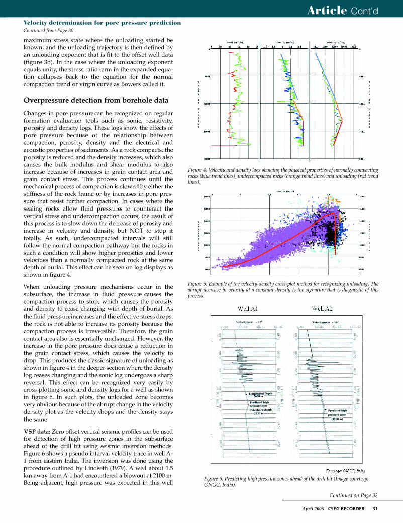
Changes in pore pre s s u re can be recognized on re g u l a rformation evaluation tools such as sonic, re s i s t i v i t y,p o rosity and density logs. These logs show the effects ofp o re pre s s u re because of the relationship betweencompaction, poro s i t y, density and the electrical andacoustic properties of sediments. As a rock compacts, thep o rosity is reduced and the density increases, which alsocauses the bulk modulus and shear modulus to alsoi n c rease because of increases in grain contact area andgrain contact stress. This process continues until themechanical process of compaction is slowed by either thes t i ffness of the rock frame or by increases in pore pre s-s u re that resist further compaction. In cases where thesealing rocks allow fluid pre s s u res to counteract thevertical stress and undercompaction occurs, the result ofthis process is to slow down the decrease of porosity andi n c rease in velocity and density, but NOT to stop itt o t a l l y. As such, undercompacted intervals will stillfollow the normal compaction pathway but the rocks insuch a condition will show higher porosities and lowervelocities than a normally compacted rock at the samedepth of burial. This effect can be seen on log displays asshown in figure 4.

When unloading pre s s u re mechanisms occur in thesubsurface, the increase in fluid pre s s u re causes thecompaction process to stop, which causes the poro s i t yand density to cease changing with depth of burial. A sthe fluid pre s s u re increases and the effective stress dro p s ,the rock is not able to increase its porosity because thecompaction process is irreversible. There f o re, the graincontact area also is essentially unchanged. However, thei n c rease in the pore pre s s u re does cause a reduction inthe grain contact stress, which causes the velocity tod rop. This produces the classic signature of unloading asshown in figure 4 in the deeper section where the densitylog ceases changing and the sonic log undergoes a sharpreversal. This effect can be recognized very easily byc ross-plotting sonic and density logs for a well as shownin figure 5. In such plots, the unloaded zone becomesvery obvious because of the abrupt change in the velocitydensity plot as the velocity drops and the density staysthe same.

VSP data: Z e ro offset vertical seismic profiles can be usedfor detection of high pre s s u re zones in the subsurfaceahead of the drill bit using seismic inversion methods.F i g u re 6 shows a pseudo interval velocity trace in well A -1 from eastern India. The inversion was done using thep ro c e d u re outlined by Lindseth (1979). A well about 1.5km away from A-1 had encountered a blowout at 2100 m.Being adjacent, high pre s s u re was expected in this well


F i g u re 4. Velocity and density logs showing the physical properties of normally compactingrocks (blue trend lines), undercompacted rocks (orange trend lines) and unloading (red tre n dl i n e s ) .

F i g u re 6. Predicting high pre s s u re zones ahead of the drill bit (Image courtesy:ONGC, India).

F i g u re 5. Example of the velocity-density cross-plot method for recognizing unloading. Theabrupt decrease in velocity at a constant density is the signature that is diagnostic of thisp ro c e s s .


Article Cont’d



also at around the same depth. VSP d a t aw e re acquired in this well and the pseudointerval velocity trace generated from thecorridor stack trace. As is evident from the‘knee’ (Fig.3), high pre s s u re was predicted at2930 m. However, due to some practical diff i-culties, drilling for this well was suspendedat 2650 m, and upto that depth no high pre s-s u re zones were encountere d .

Another well A-2, about 2 km away from A -1 was drilled (depth not available) and VSPdata was acquired and processed. The ‘knee’seen on the pseudo interval velocity traceindicated that high pre s s u re was to beexpected at 3200 m. Drilling was continuedfurther and high pre s s u re was encountere dat 3180 m in accordance with the pre d i c t i o n .At the time this work was done, pre s s u reindications were read off from the intervalvelocity traces

Overpressure detection from seismic data

The estimation of pore pre s s u res fro mseismic data uses seismically-derivedvelocities to infer the subsurface formationpore pressure. The Eaton method uses adirect transform from velocity to pore pres-sure, while the Bowers method estimatesthe effective stress from the velocities andthen calculates the pore pressure. There aremany different types of seismic velocities,but only those velocities that are dense andaccurate and are close to the formationvelocity under consideration, will be ofinterest. The following methods have beenused with varying degrees of success andwill be discussed individually.

1. Dense velocity analysis.

2. Geologically consistent velocity analysis.

3. Horizon-keyed velocity analysis.

4. Automated velocity analysis.

5. Velocity determination using reflectiontomography.

6. Residual velocity analysis.

7. Velocities from seismic inversion.

B e f o re discussing these methods, some-thing must be said about data conditioningfor geopressure.

Data ConditioningVelocity analysis for geopre s s u re pre d i c t i o nre q u i res a level of detail in the velocityanalysis that goes beyond the normalstacking velocity approaches used for tradi-tional imaging work. Imaging velocityanalysis usually results in a highlysmoothed velocity field that is designed toF i g u re 9. Traditional semblance-based velocity analysis display showing under-corrected gather (left) and an

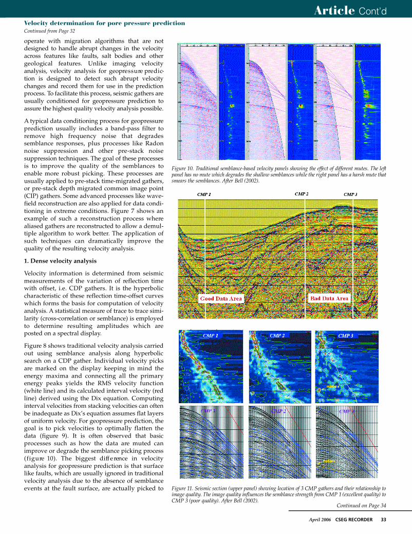
o v e r - c o r rected gather (right) compared to the properly flattened gather (middle). After Bell (2002).

F i g u re 8. Traditional semblance-based velocity analysis display showing a semblance panel (left), un-corre c t e dgather (middle panel) and NMO-corrected gather (right panel). After Bell (2002).

F i g u re 7. Example of advanced wavefield reconstruction to eliminate aliasing of pre-stack data for impro v e dvelocity analysis and imaging. The water-bottom multiples in panel A a re severely aliased which degrades thequality of the radon demultiple (panel C). After wavefield reconstruction (panel B), the multiples can be re m o v e dm o re robustly (panel D).


Article Cont’d

operate with migration algorithms that are notdesigned to handle abrupt changes in the velocitya c ross features like faults, salt bodies and othergeological features. Unlike imaging velocityanalysis, velocity analysis for geopre s s u re pre d i c-tion is designed to detect such abrupt velocitychanges and re c o rd them for use in the pre d i c t i o np rocess. To facilitate this process, seismic gathers areusually conditioned for geopre s s u re prediction toa s s u re the highest quality velocity analysis possible.

A typical data conditioning process for geopressureprediction usually includes a band-pass filter toremove high frequency noise that degradessemblance responses, plus processes like Radonnoise suppression and other pre-stack noisesuppression techniques. The goal of these processesis to improve the quality of the semblances toenable more robust picking. These processes areusually applied to pre-stack time-migrated gathers,or pre-stack depth migrated common image point(CIP) gathers. Some advanced processes like wave-field reconstruction are also applied for data condi-tioning in extreme conditions. Figure 7 shows anexample of such a reconstruction process wherealiased gathers are reconstructed to allow a demul-tiple algorithm to work better. The application ofsuch techniques can dramatically improve thequality of the resulting velocity analysis.

1. Dense velocity analysis

Velocity information is determined from seismicmeasurements of the variation of reflection timewith offset, i.e. CDP gathers. It is the hyperboliccharacteristic of these reflection time-offset curveswhich forms the basis for computation of velocityanalysis. A statistical measure of trace to trace simi-larity (cross-correlation or semblance) is employedto determine resulting amplitudes which areposted on a spectral display.

Figure 8 shows traditional velocity analysis carriedout using semblance analysis along hyperbolicsearch on a CDP gather. Individual velocity picksare marked on the display keeping in mind theenergy maxima and connecting all the primaryenergy peaks yields the RMS velocity function(white line) and its calculated interval velocity (redline) derived using the Dix equation. Computinginterval velocities from stacking velocities can oftenbe inadequate as Dix’s equation assumes flat layersof uniform velocity. For geopressure prediction, thegoal is to pick velocities to optimally flatten thedata (figure 9). It is often observed that basicprocesses such as how the data are muted canimprove or degrade the semblance picking process( f i g u re 10). The biggest diff e rence in velocityanalysis for geopressure prediction is that surfacelike faults, which are usually ignored in traditionalvelocity analysis due to the absence of semblanceevents at the fault surface, are actually picked to


F i g u re 11. Seismic section (upper panel) showing location of 3 CMP gathers and their relationship toimage quality. The image quality influences the semblance strength from CMP 1 (excellent quality) toCMP 3 (poor quality). After Bell (2002).

F i g u re 10. Traditional semblance-based velocity panels showing the effect of different mutes. The leftpanel has no mute which degrades the shallow semblances while the right panel has a harsh mute thatsmears the semblances. After Bell (2002).


F i g u re 12 (a). Cross-section through the final velocity model, (b). Cross-section through the calibrated pore pre s s u re gradient volume. (After Snijder et al., 2003).

F i g u re 13 (a). Interval velocity map before and after velocity refinement and calibration, (b). Computed pore pre s s u re overlaying the seismic data. (After Caudron et al., 2003).


assure that velocity changes across the fault are honored. It isalso often observed that the quality of velocity analysis is directlyaffected by the quality of the underlying imaging. Figure 11shows an example of 3 CDP’s on a seismic line with variable dataquality. This example shows how significant the image quality isfor good velocity analysis.

Example 1Traditional stacking velocities have been used to construct pre s s u rep rediction cubes that provide new insights into the 3D subsurfacep re s s u re distribution. Figure 12 (a) shows a cross-section through afinal velocity volume from the Columbus Basin, off s h o re Tr i n i d a d& Tobago (Snijder et al., 2002). An interval velocity cube was firstgenerated from DMO velocity functions and DMO velocities slicesgenerated along 150 ms thick time slices parallel to the sea bed.Next, the DMO velocities were converted into interval velocitiesusing Dix formula and smoothed using a 3000m running averagef i l t e r. These smooth interval velocity slices were used to convert thetime slices into depth and generate the seismic interval velocitycube with respect to depth. The horizons tracked on the seismictime volume were converted to depth using the smoothed velocityfunction and overlayed on the interval velocity depth volume. Therather large mismatches between this modelled velocity and welldata were minimized by applying the first-order laterally variablevelocity correction map to the velocity cube.

Actual measurements carried out in wells like RFT, MDT and mudweights etc. were next used to perform a final calibration ofp redicted pre s s u re to actual pre s s u res via cross-plots. A c o n s i s t e n tbias found was removed by using a simple linear corre c t i o n .

F i g u re 12(b) shows a cross-section through the calibrated pore pre s-s u re gradient volume. More details about the method and itsimplementation can be picked up from the re f e rence cited above.

Example 2This example is from the Macuspana Basin, located at the northof the Montagua-Polochic fault system in South Mexico(Caudron et al., 2003). Complex shale tectonics has complicatedthe basin’s geological structure setting and presents a challengefor petroleum exploration and production. Drilling in the areahas confirmed compartmentalization of pore pressures, which isassociated with the complex structure.

RMS velocity functions were picked on a grid of 20 x 20 (inlinesx crosslines) for use in 3D prestack time migrated gathers. Thequality of the seismic data and the complex nature of the struc-tures being investigated suggested manual residual moveoutpicking so as to refine the RMS velocity to a grid of 5 x 5 (150m x150m). Next, the velocity field was calibrated with well log data.

Figure 13(a) shows a comparison of an interval velocity map at adepth of 3000 m before and after the velocity refinement and cali-bration. Clearly, more detailed velocity changes can be seen onthe refined interval velocity map.

Figure 13(b) shows the pore pressure overlaying the seismicdata. The growth fault in red and the fault in yellow on thedisplay appear to be pressure boundaries. Apparently, the highcompartmentalized pressure distribution has been influenced bythe pattern of the fault system. The growth faults might haveprevented the expulsion of water from the pores of sedimentsduring compaction and diagenesis.

Article Cont’dVelocity determination for pore pressure prediction Continued from Page 33


a) b)

a)

b)

2. Geologically consistent velocity analysis

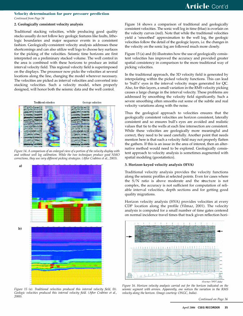
Traditional stacking velocities, while producing good qualitystacks usually do not follow key geologic features like faults, litho-logic boundaries and major sequence events in a consistentfashion. Geologically-consistent velocity analysis addresses theseshortcomings and can also utilize well logs to choose key surfacesfor the picking of the velocities. Seismic time horizons are firsti n t e r p reted on a preliminary stacked volume. The well control inthe area is combined with these horizons to produce an initialinterval velocity field. This regional velocity field is superimposedon the displays. The processor now picks the velocities at severallocations along the line, changing the model wherever necessary.The velocities are picked as interval velocities and converted intostacking velocities. Such a velocity model, when pro p e r l ydesigned, will honor both the seismic data and the well contro l .

F i g u re 14 shows a comparison of traditional and geologicallyconsistent velocities. The sonic well log in time (blue) is overlain onthe velocity curves (red). Note that while the traditional velocitiesyield a ‘smoothed’ approximation to the well log, the geologicvelocities follow the detail of the geologic layers, i.e. the changes inthe velocity on the sonic log are followed much more closely.

F i g u re 15 (a) and (b) illustrates how the use of geologically consis-tent velocities has improved the accuracy and provided gre a t e rspatial consistency in comparison to the more traditional way ofpicking velocities.

In the traditional approach, the 3D velocity field is generated byinterpolating within the picked velocity functions. This can leadto ‘bull’s’ eyes in the interval velocity maps generated for QC.Also, for thin layers, a small variation in the RMS velocity pickingcauses a large change in the interval velocity. These problems area d d ressed by smoothing the velocity field significantly. Such as e v e re smoothing often smooths out some of the subtle and re a lvelocity variations along with the noise.

Thus the geological approach to velocities ensures that thegeologically consistent velocities are horizon consistent, laterallyconsistent and so ensures bull’s eyes are avoided and re a l i s t i cvalues that tie to the wells at each line intersection are consistent.While these velocities are geologically more meaningful andc o r rect, they need to be used care f u l l y. Another point that needsmention here is that such a velocity field may not properly flattenthe gathers. If this is an issue in the area of interest, then an alter-native method would need to be explored. Geologically consis-tent approach to velocity analysis is sometimes augmented withspatial modeling (geostatistics).

3. Horizon-keyed velocity analysis (HVA)

Traditional velocity analysis provides the velocity functionsalong the seismic profiles at selected points. Even for cases wherethe S/N ratio is above moderate and the stru c t u re is notcomplex, the accuracy is not sufficient for computation of reli-able interval velocities, depth sections and for getting goodquality migrations.

Horizon velocity analysis (HVA) provides velocities at everyCDP location along the profile (Yilmaz, 2001). The velocityanalysis is computed for a small number of time gates centeredon normal incidence travel times that track given reflection hori-




F i g u re 14. A comparison of an enlarged view of a portion of the velocity display withand without well log calibration. While the two techniques produce good NMOc o r rections, they use very different picking strategies. (After Crabtree et al., 2003).

F i g u re 15 (a). Traditional velocities produced this interval velocity field, (b).Geologic velocities produced this interval velocity field. (After Crabtree et al.,2 0 0 0 ) .

F i g u re 16. Horizon velocity analysis carried out for the horizon indicated on theseismic segment with arrows. Appare n t l y, one notices the variation in the RMSvelocity along the horizon. (Image courtesy: ONGC, India).

a)

b)


zons. Since only a few time gates are to be considered and therange of trial velocities is limited, the computer time is used in abetter way in conducting an intensive analysis on importantevents, than on time zones between horizons.

Figure 16 shows a reflecting horizon and its associated computedHVA. Once HVA computation is completed for the main hori-zons in the section, it is possible to build up a grid by computingthe interval velocity between these main horizons.

Horizon velocity analysis can provide high spatial resolution butthe temporal resolution may be low for pore pressure predictionapplications. Due to this reason, this approach should be appliedin conjunction with another technique where this informationproves useful.

4. Automated velocity inversion

An automated velocity inversion technique has been proposed byMao et al., 2000 in which stacking velocities are assumed equiva-lent to RMS velocities, an assumption that would re q u i re appro-priate corrections for reflector dip, non-hyperbolic moveout andevent timing. Such assumptions can only be satisfied with pre s t a c kdepth migration as demonstrated by Deregowski 1990. The datainput to this method are migrated image gathers. The methodcomprises a series of algorithmic components:

( 1 )As the first step, reflection events in 3D space are first analysed.Those events and their corresponding stacking velocities thatexhibit maximum spatial consistency are picked.

( 2 )Next, treating the stacking velocities as RMS velocities andusing a least-squares optimisation pro c e d u re constrainedinterval velocities are computed.

( 3 )These velocities are then smoothed using a cascaded medianf i l t e r, keeping in mind the desired resolution limits in terms ofthe magnitude and the lateral extent of the smallest velocityanomaly to be resolved.

The method yields a 3D velocity model in which steep dips and relatively rapid velocity variations have been handled (Maoet al., 2003).

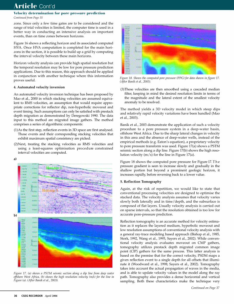
Banik et al., 2003 demonstrate the application of such a velocityprocedure to a pore pressure system in a deep-water basin,offshore West Africa. Due to the sharp lateral changes in velocityin this area and the absence of deep-water wells, instead of theempirical methods (e.g. Eaton’s equation), a proprietary velocityto pore pressure transform was used. Figure 17(a) shows a PSTMseismic section along a dip line. Figure 17(b) shows the high reso-lution velocity (m/s) for the line in Figure 17(a).

Figure 18 shows the computed pore pressure for Figure 17. T h ep re s s u re gradient is seen to increase slowly and gradually in theshallow portion but beyond a prominent geologic horizon, iti n c reases rapidly, before reversing back to a lower value.

5. Reflection Tomography

Again, at the risk of repetition, we would like to state thatconventional processing velocities are designed to optimise thestacked data. The velocity analysis assumes that velocity variesslowly both laterally and in time/depth, and the subsurface iscomposed of flat layers. Usually velocity analysis is carried outon sparse intervals, so that the resolution obtained is too low foraccurate pore-pressure prediction.

Reflection tomography is an accurate method for velocity estima-tion as it replaces the layered medium, hyperbolic moveout andlow resolution assumptions of conventional velocity analysis witha general ray-trace modeling based approach (Bishop et al., 1985,Stork, 1992, Wang et al., 1995, Sayers et al., 2002). While conven-tional velocity analysis evaluates moveout on CMP g a t h e r s ,tomography utilizes prestack depth migrated common imagepoint (CIP) gathers for the same process. This latter analysis isbased on the premise that for the correct velocity, PSDM maps agiven reflection event to a single depth for all offsets that illumi-nate it (Wo o d w a rd et al., 1998; Sayers et al., 2002). To m o g r a p h ytakes into account the actual propagation of waves in the media,and is able to update velocity values in the model along the raypath. Tomography also provides a dense horizontal and verticalsampling. Both these characteristics make the technique very



F i g u re 18. Shows the computed pore pre s s u re (PPG) for data shown in figure 17.(After Banik et al., 2003).

F i g u re 17. (a) shows a PSTM seismic section along a dip line from deep watero f f s h o re West Africa, (b) shows the high resolution velocity (m/s) for the line inF i g u re (a). (After Banik et al., 2003).

a)

b)

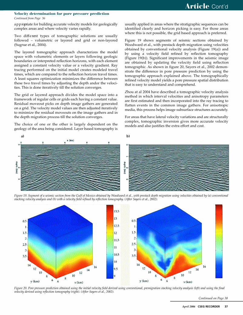
F i g u re 19. Segment of a seismic section from the Gulf of Mexico obtained by Woodward et al., with prestack depth migration using velocities obtained by (a) conventionalstacking velocity analysis and (b) with a velocity field refined by reflection tomography. (After Sayers et al., 2002).

a) b)

F i g u re 20. Pore pre s s u re prediction obtained using the initial velocity field derived using conventional, premigration stacking velocity analysis (left) and using the finalvelocity derived using reflection tomography (right). (After Sayers et al., 2002).




a p p ropriate for building accurate velocity models for geologicallycomplex areas and where velocity varies rapidly.

Two diff e rent types of tomographic solutions are usuallyfollowed – volumetric or layered and grid or non-layere d(Sugrue et al., 2004).

The layered tomographic approach characterizes the modelspace with volumetric elements or layers following geologicboundaries or interpreted reflection horizons, with each elementassigned a constant velocity value or a velocity gradient. Raytracing performed on the initial model creates modeled traveltimes, which are compared to the reflection horizon travel times.A least squares optimization minimizes the difference betweenthese two travel times by adjusting the depth andor the veloci-ties. This is done iteratively till the solution converges.

The grid or layered approach divides the model space into aframework of regular cells or grids each having a constant value.Residual moveout picks on depth image gathers are generatedon a grid. The velocity model values are then adjusted iterativelyto minimize the residual moveouts on the image gathers and inthe depth migration process till the solution converges.

The choice of one or the other is largely dependent on thegeology of the area being considered. Layer based tomography is

usually applied in areas where the stratigraphic sequences can beidentified clearly and horizon picking is easy. For those areaswhere this is not possible, the grid based approach is preferred.

F i g u re 19 shows segments of seismic sections obtained byWoodward et al., with prestack depth migration using velocitiesobtained by conventional velocity analysis (Figure 19(a)) and by using a velocity field refined by reflection tomography(Figure 19(b)). Significant improvements in the seismic image are obtained by updating the velocity field using reflection tomographic. As shown in figure 20, Sayers et al., 2002 demon-strate the difference in pore pressure prediction by using thetomographic approach explained above. The tomographicallyrefined velocity model yields a pore pressure spatial distributionthat is easy to understand and comprehend.

Zhou at al 2004 have described a tomographic velocity analysismethod in which interval velocities and anisotropy parametersare first estimated and then incorporated into the ray tracing toflatten events in the common image gathers. For anisotropicmedia, this process helps image subsurface structures accurately.

For areas that have lateral velocity variations and are structurallycomplex, tomographic inversion gives more accurate velocitymodels and also justifies the extra effort and cost.


6. Residual velocity analysis

One of the serious problems in doing AVO analysis isobtaining precise stacking velocity measurements for itsproper application. Velocity errors that have little to no affecton conventional stacking can cause significant AVO variationseveral times larger than those predicted by theory (Spratt,1987). Shuey’s formulation for AVO yields an intercept and agradient stack. While the intercept represents the zero offsetreflection coefficients, the gradient is a measure of the offsetdependent re f l e c t i v i t y. Swan, 2001 studied the effect ofresidual velocity on the gradient and developed a method-ology to minimize the errors by utilizing a new AVO productindicator which he called the Residual Velocity Indicator(RVI). This indicator equals the product of AVO zero offsetstack and the phase quadrature of the gradient. The sign of thecorrelation indicates whether the NMO velocity is too high ortoo low. The optimal NMO velocity is the one which mini-mizes this RVI correlation. Residual velocity analysisproduces a null point at every sample point, which facilitatesthe generation of a velocity value at every data sample. Thusa high resolution velocity field is generated. So, while tradi-tional stacking velocities are generally picked withsemblances, optimum velocities for AVO are picked usingRVI, which is more sensitive to velocity variations than a stan-d a rd semblance estimate. The residual velocity method,which was popularized by ARCO with the AVEL algorithm,also allows accurate prediction of velocities in the presence oftype II polarity-reversing AVO events which cause problemsfor traditional semblance analysis. Spatial and temporal aver-aging forms part of the process to obtain a smooth and acontinuous residual velocity estimate.

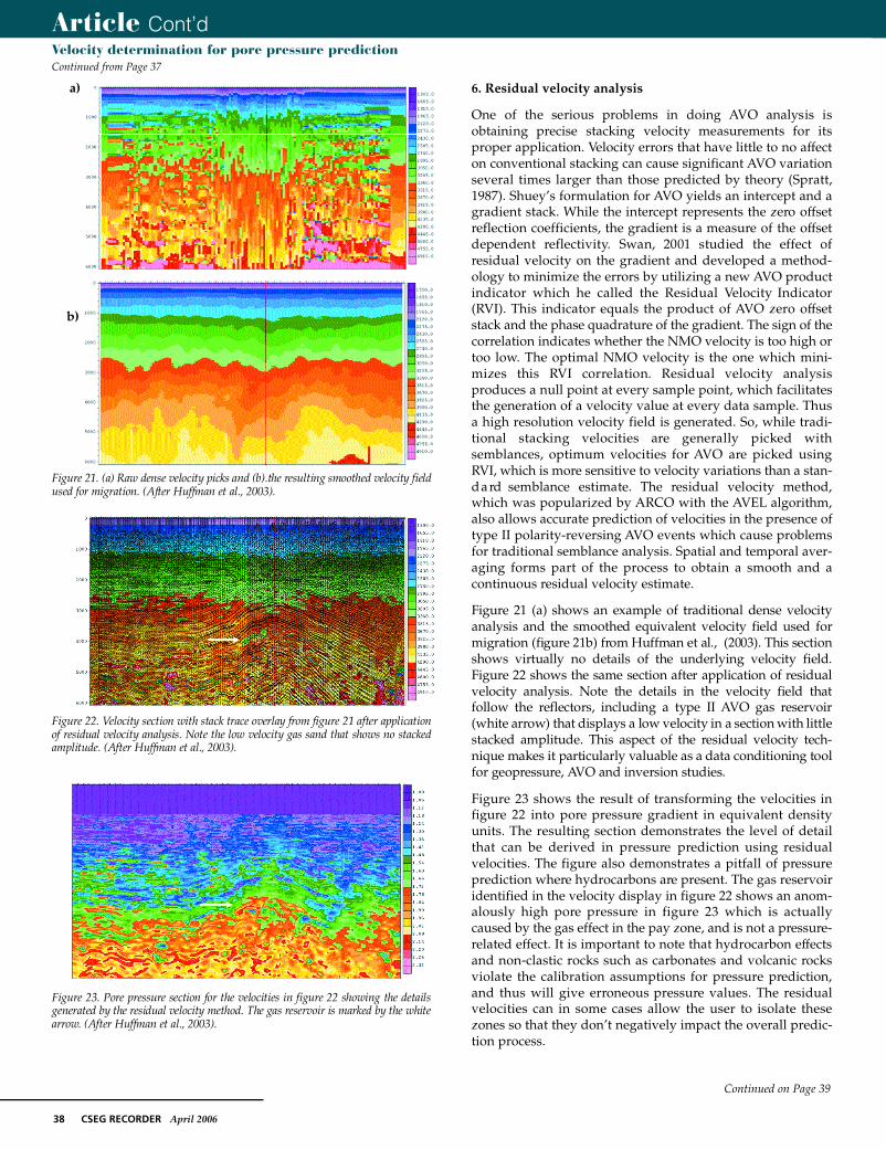
F i g u re 21 (a) shows an example of traditional dense velocityanalysis and the smoothed equivalent velocity field used formigration (figure 21b) from Huffman et al., (2003). This sectionshows virtually no details of the underlying velocity field.F i g u re 22 shows the same section after application of re s i d u a lvelocity analysis. Note the details in the velocity field thatfollow the reflectors, including a type II AVO gas re s e r v o i r(white arrow) that displays a low velocity in a section with littlestacked amplitude. This aspect of the residual velocity tech-nique makes it particularly valuable as a data conditioning toolfor geopre s s u re, AVO and inversion studies.

Figure 23 shows the result of transforming the velocities infigure 22 into pore pressure gradient in equivalent densityunits. The resulting section demonstrates the level of detailthat can be derived in pressure prediction using residualvelocities. The figure also demonstrates a pitfall of pressureprediction where hydrocarbons are present. The gas reservoiridentified in the velocity display in figure 22 shows an anom-alously high pore pressure in figure 23 which is actuallycaused by the gas effect in the pay zone, and is not a pressure-related effect. It is important to note that hydrocarbon effectsand non-clastic rocks such as carbonates and volcanic rocksviolate the calibration assumptions for pressure prediction,and thus will give erroneous pressure values. The residualvelocities can in some cases allow the user to isolate thesezones so that they don’t negatively impact the overall predic-tion process.



F i g u re 22. Velocity section with stack trace overlay from figure 21 after applicationof residual velocity analysis. Note the low velocity gas sand that shows no stackedamplitude. (After Huffman et al., 2003).

F i g u re 23. Pore pre s s u re section for the velocities in figure 22 showing the detailsgenerated by the residual velocity method. The gas reservoir is marked by the whitea r ro w. (After Huffman et al., 2003).

F i g u re 21. (a) Raw dense velocity picks and (b).the resulting smoothed velocity fieldused for migration. (After Huffman et al., 2003).

a)

b)




The computation of residual velocities uses a number of assump-tions, an important one being that the velocity is assumed asconstant and that AVO behaviour is consistent in the RVI window.Short offset for moveout and AVO analysis is another assumption.R a t c l i ff and Roberts (2003) showed that these and other assump-tions are often invalid in real data and this adds noise and insta-bility to the iteration process. By monitoring the converg e n c ecriteria it is possible to reduce or avoid these instabilities.

Ratcliff and Roberts extended Swan’s method in that once RVIestimates are computed, they are used to update the velocityfield and any subsequent moveout correction. AVO analysis isrepeated on the revised gathers and another residual velocity iscalculated. This process is iterated until convergence occurs. Thisreduces the side effects mentioned above.

7. Velocities from Seismic Inversion

Seismic inversion plays an important role in seismic interpreta-tion, reservoir characterization, time lapse seismic, pressureprediction and other geophysical applications. Usually, the termseismic inversion refers to transformation of post-stack or pre-stack seismic data into acoustic impedance inversion. Becauseacoustic impedance is a layer property, it simplifies lithologicand stratigraphic identification and may be directly converted tolithologic or reservoir properties such as pseudo velocity,porosity, fluid fill and net pay. In such cases, inversion allowsd i rect interpretation of three-dimensional geobodies. Forgeopressure prediction, inversion can be implemented as ameans to refine the velocity field beyond the resolution ofresidual velocity analysis, and also as a means to separateunwanted data from the pressure calculations.

The pre f e r red methodology for implementing inversion forg e o p re s s u re prediction is to start with a 3D residual velocity field(e.g. figure 21b) that can be used as a low-frequency velocity fieldto seed the inversion. The inversion is then used to refine thevelocity field using the reflectivity information contained in thestacked data or gathers to provide the high-frequency velocityfield.

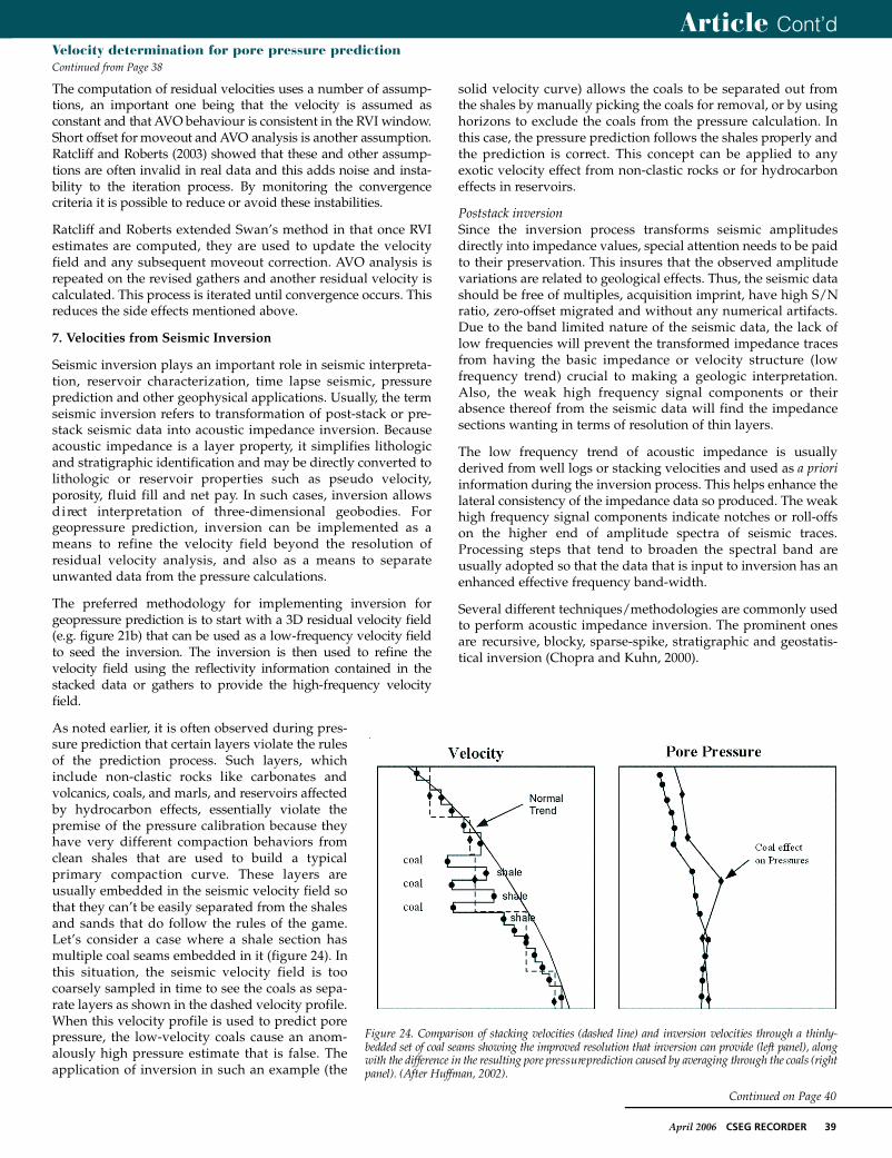
As noted earlier, it is often observed during pres-sure prediction that certain layers violate the rulesof the prediction process. Such layers, whichinclude non-clastic rocks like carbonates andvolcanics, coals, and marls, and reservoirs affectedby hydrocarbon effects, essentially violate thepremise of the pressure calibration because theyhave very different compaction behaviors fromclean shales that are used to build a typicalprimary compaction curve. These layers areusually embedded in the seismic velocity field sothat they can’t be easily separated from the shalesand sands that do follow the rules of the game.Let’s consider a case where a shale section hasmultiple coal seams embedded in it (figure 24). Inthis situation, the seismic velocity field is toocoarsely sampled in time to see the coals as sepa-rate layers as shown in the dashed velocity profile.When this velocity profile is used to predict porepressure, the low-velocity coals cause an anom-alously high pressure estimate that is false. Theapplication of inversion in such an example (the

solid velocity curve) allows the coals to be separated out fromthe shales by manually picking the coals for removal, or by usinghorizons to exclude the coals from the pressure calculation. Inthis case, the pressure prediction follows the shales properly andthe prediction is correct. This concept can be applied to anyexotic velocity effect from non-clastic rocks or for hydrocarboneffects in reservoirs.

Poststack inversionSince the inversion process transforms seismic amplitudesdirectly into impedance values, special attention needs to be paidto their preservation. This insures that the observed amplitudevariations are related to geological effects. Thus, the seismic datashould be free of multiples, acquisition imprint, have high S/Nratio, zero-offset migrated and without any numerical artifacts.Due to the band limited nature of the seismic data, the lack oflow frequencies will prevent the transformed impedance tracesfrom having the basic impedance or velocity structure (lowfrequency trend) crucial to making a geologic interpretation.Also, the weak high frequency signal components or theirabsence thereof from the seismic data will find the impedancesections wanting in terms of resolution of thin layers.

The low frequency trend of acoustic impedance is usuallyderived from well logs or stacking velocities and used as a prioriinformation during the inversion process. This helps enhance thelateral consistency of the impedance data so produced. The weakhigh frequency signal components indicate notches or roll-offson the higher end of amplitude spectra of seismic traces.Processing steps that tend to broaden the spectral band areusually adopted so that the data that is input to inversion has anenhanced effective frequency band-width.

Several different techniques/methodologies are commonly usedto perform acoustic impedance inversion. The prominent onesare recursive, blocky, sparse-spike, stratigraphic and geostatis-tical inversion (Chopra and Kuhn, 2000).

F i g u re 24. Comparison of stacking velocities (dashed line) and inversion velocities through a thinly-bedded set of coal seams showing the improved resolution that inversion can provide (left panel), alongwith the difference in the resulting pore pre s s u re prediction caused by averaging through the coals (rightpanel). (After Huffman, 2002).


All the above model based inversion methods belongs to a cate-gory called local optimization methods. A common characteristic isthat they iteratively adjust the subsurface model in such a waythat the misfit function (between synthetic and actual data)decreases monotonically. In the case of good well control, thestarting model is good and so the local optimization methodsproduce satisfactory results. For sparse well control or where thecorrelation between seismic events and nearby well control ismade difficult by fault zones, thinning of beds, local disappear-ance of impedance contrast or the presence of noise, thesemethods do not work satisfactorily. In such cases global opti-mization methods, e.g. simulated annealing, needs to be used.Global optimization methods employ statistical techniques andgive reasonably accurate results.

Thus whatever inversion approach is adopted i.e. constrained, strati-graphic, the acoustic impedance volumes so generated have signifi-cant advantages. These include increased frequency bandwidth,enhanced resolution and reliability of amplitude interpre t a t i o nt h rough detuning of seismic data and obtaining a layer property thata ff o rds convenience in understanding and interpre t a t i o n .

Prestack inversionWhile poststack seismic inversion is being used routinely thesedays, the results can be viewed with suspicion due to theinherent problem of uniqueness in terms of lithology and fluiddiscrimination. Variations in acoustic impedance could resultfrom a combination of many factors like lithology, porosity, fluidcontent and saturation or pore pressure. Prestack inversion helpsin reducing this ambiguity, as it can generate not only compres-sional but shear information for the rocks under consideration.For example, for a gas sand a lowering of compressional velocityand a slight increase in shear velocity is encountered, ascompared with a brine-saturated sandstone. Prestack inversionproves useful in such cases.

The commonly used prestack inversion methods, aimed atdetecting lithology and fluid content, derive the AVO interceptand AVO gradient (Shuey, 1985) or normal incident reflectivityand Poisson reflectivity (Verm and Hilterman, 1995) or P-and S-reflectivities (Fatti et al., 1994). Fatti’s approach makes noassumption about the Vp/Vs and density and is valid for inci-dent angles upto 50 degrees. The AVO derived reflectivities areusually inverted individually to determine rock properties forthe respective rock layers. The accuracy and resolution of rockproperty estimates depend to a large extent on the inversionmethod utilized.

A joint or simultaneous inversion flow may simultaneouslytransform the P- and S- reflectivity data (Ma, 2001) into acousticand shear impedances or it may simultaneously invert for rockproperties starting from prestack P-wave offset seismic gathers(Ma, 2002). Simultaneous inversion methodology extracts anenhanced dynamic range of data from offset seismic stacks,resulting in an improved response for reservoir characterizationover traditional post stack or AVO analysis (Fowler et al., 2002).

Prestack inversion for rock properties has been addressed latelyusing global optimization algorithms (Sen and Stoffa, 1991,Mallick, 1995, Ma, 2001, Ma, 2002). In these model-driven inver-sion methods, synthetic data are generated using an initialsubsurface model and compared to real seismic data; the model

is modified and synthetic data are updated and compared to thereal data again. If after a number of iterations no furtherimprovement is achieved, the updated model is the inversionresult. Some constraints can be incorporated to reduce the non-uniqueness of the output. These methods utilize a Monte Carlorandom approach and effectively find a global minimumwithout making assumptions about the shape of the objectivefunction and are independent of the starting models.

Mallick (1999) presented a prestack inversion method using agenetic algorithm to find the P- and S- velocity models by mini-mizing the misfit between observed angle gathers and theirsynthetic computations. On the Woodbine gas sand dataset fromEast Texas, he showed a comparison of prestack inversion withpost stack recursive inversion, and demonstrated that prestackinversion showed detailed stratigraphic features of the subsur-face not seen on the post stack inversion. This method iscomputer intensive but the superior quality of the results justi-fies rthe need for such an inversion.

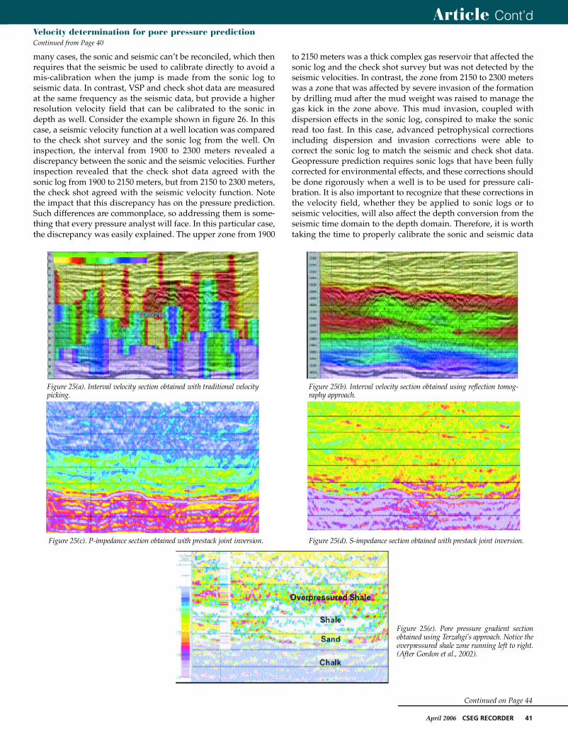
ExampleThe sonic and velocity log-derived porosity trends from offshoreIreland suggest overpressures within Tertiary shale sequences.Analysis of seismic velocities for this area suggest normal shalecompaction for most of the Tertiary overburden, except in certainlithologies where overcompaction is seen. The stacking velocitiespicked on a coarse grid and were not horizon consistent, so lookblocky as shown in Figure 25(a). If there are lateral velocity vari-ations, as seen in this case, this approach is not suitable for porepressure analysis. In order to obtain accurate and high resolutionseismically derived velocities, several iterations of the prestackdepth migration using tomography was attempted. The gridbased tomography provides an optimum seismic image as wellas the velocity section shown in Fig. 25(b) corresponding to Fig.25(a). Next prestack seismic inversion was attempted using Ma’s(2001) approach to be able to predict different lithologies in termsof P- and S- impedances and the two equivalent sections areshown in Fig. 25(c) and (d).

Terzaghi’s effective principle was then used to transform theseismic inversion derived impedance to pore pressure. Theequivalent section shown in Fig. 25 (e) shows overpressuredshales as anticipated in this area. Such information providesassurance for development well locations.

Discrepancies Between Wellbore and Seismic VelocitiesOne of the challenges in performing geopressure prediction withseismic velocities is that the seismic and wellbore velocities oftendo not calibrate properly against each other. When this occurs, anobvious question arises regarding which data type provides thebest base calibration for geopressure. While this topic is beyondthe general scope of this review, a few words should be saidabout this important topic. The issue not only affects the calibra-tion for pressure, but also has an impact on the time-depthconversion that is required to equate the seismic velocities intime to pressure profiles in depth that are used for drilling wells.

While sonic velocities provide the highest resolution of the avail-able velocity data, the sonic velocities often don’t provide thebest calibration for seismic-based prediction because of differ-ences in the frequency of measurement compared to seismic dataand due to invasion and other deleterious wellbore effects. In




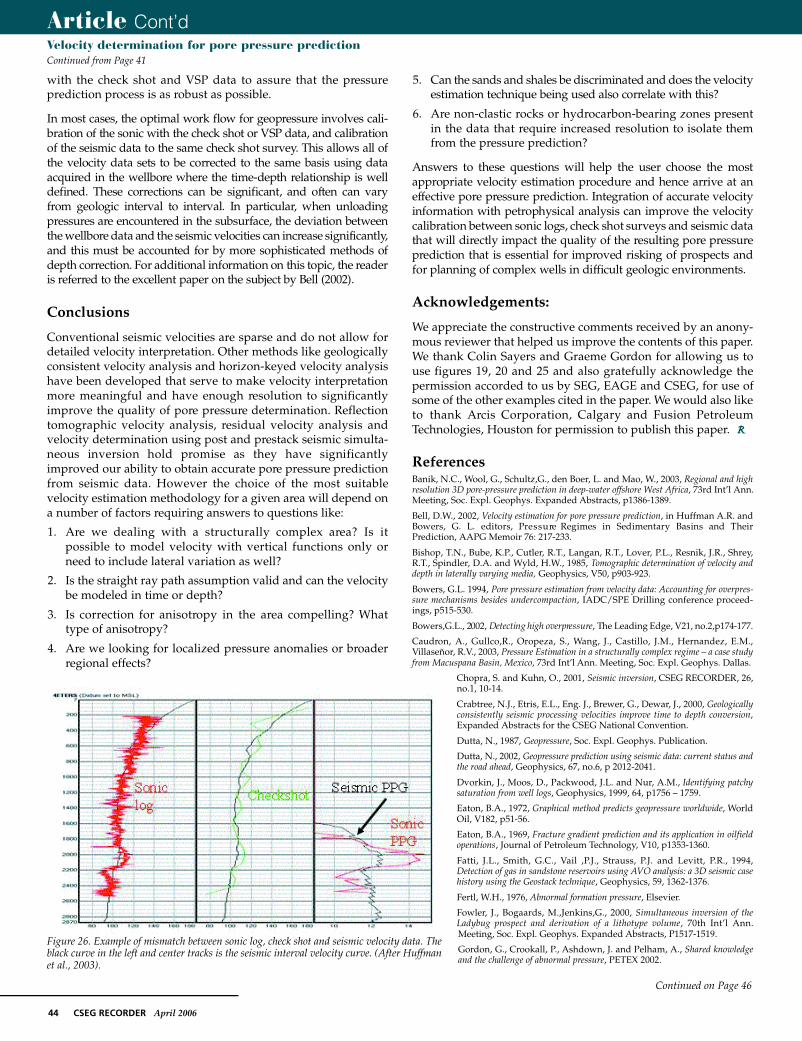
many cases, the sonic and seismic can’t be reconciled, which thenrequires that the seismic be used to calibrate directly to avoid amis-calibration when the jump is made from the sonic log toseismic data. In contrast, VSP and check shot data are measuredat the same frequency as the seismic data, but provide a higherresolution velocity field that can be calibrated to the sonic indepth as well. Consider the example shown in figure 26. In thiscase, a seismic velocity function at a well location was comparedto the check shot survey and the sonic log from the well. Oninspection, the interval from 1900 to 2300 meters revealed adiscrepancy between the sonic and the seismic velocities. Furtherinspection revealed that the check shot data agreed with thesonic log from 1900 to 2150 meters, but from 2150 to 2300 meters,the check shot agreed with the seismic velocity function. Notethe impact that this discrepancy has on the pressure prediction.Such differences are commonplace, so addressing them is some-thing that every pressure analyst will face. In this particular case,the discrepancy was easily explained. The upper zone from 1900

to 2150 meters was a thick complex gas reservoir that affected thesonic log and the check shot survey but was not detected by theseismic velocities. In contrast, the zone from 2150 to 2300 meterswas a zone that was affected by severe invasion of the formationby drilling mud after the mud weight was raised to manage thegas kick in the zone above. This mud invasion, coupled withdispersion effects in the sonic log, conspired to make the sonicread too fast. In this case, advanced petrophysical correctionsincluding dispersion and invasion corrections were able tocorrect the sonic log to match the seismic and check shot data.Geopressure prediction requires sonic logs that have been fullycorrected for environmental effects, and these corrections shouldbe done rigorously when a well is to be used for pressure cali-bration. It is also important to recognize that these corrections inthe velocity field, whether they be applied to sonic logs or toseismic velocities, will also affect the depth conversion from theseismic time domain to the depth domain. Therefore, it is worthtaking the time to properly calibrate the sonic and seismic data



F i g u re 25(a). Interval velocity section obtained with traditional velocityp i c k i n g .

F i g u re 25(b). Interval velocity section obtained using reflection tomog-raphy appro a c h .

F i g u re 25(c). P-impedance section obtained with prestack joint inversion.

F i g u re 25(e). Pore pre s s u re gradient sectionobtained using Te r z a h g i ’s approach. Notice theo v e r p re s s u red shale zone running left to right.(After Gordon et al., 2002).

F i g u re 25(d). S-impedance section obtained with prestack joint inversion.


with the check shot and VSP data to assure that the pressureprediction process is as robust as possible.

In most cases, the optimal work flow for geopre s s u re involves cali-bration of the sonic with the check shot or VSP data, and calibrationof the seismic data to the same check shot survey. This allows all ofthe velocity data sets to be corrected to the same basis using dataa c q u i red in the wellbore where the time-depth relationship is welldefined. These corrections can be significant, and often can varyf rom geologic interval to interval. In particular, when unloadingp re s s u res are encountered in the subsurface, the deviation betweenthe wellbore data and the seismic velocities can increase significantly,and this must be accounted for by more sophisticated methods ofdepth correction. For additional information on this topic, the re a d e ris re f e r red to the excellent paper on the subject by Bell (2002).

Conclusions

Conventional seismic velocities are sparse and do not allow fordetailed velocity interpretation. Other methods like geologicallyconsistent velocity analysis and horizon-keyed velocity analysishave been developed that serve to make velocity interpretationmore meaningful and have enough resolution to significantlyimprove the quality of pore pressure determination. Reflectiontomographic velocity analysis, residual velocity analysis andvelocity determination using post and prestack seismic simulta-neous inversion hold promise as they have significantlyimproved our ability to obtain accurate pore pressure predictionfrom seismic data. However the choice of the most suitablevelocity estimation methodology for a given area will depend ona number of factors requiring answers to questions like:

1. Are we dealing with a structurally complex area? Is itpossible to model velocity with vertical functions only orneed to include lateral variation as well?

2. Is the straight ray path assumption valid and can the velocitybe modeled in time or depth?

3. Is correction for anisotropy in the area compelling? Whattype of anisotropy?

4. Are we looking for localized pressure anomalies or broaderregional effects?

5. Can the sands and shales be discriminated and does the velocityestimation technique being used also correlate with this?

6. Are non-clastic rocks or hydrocarbon-bearing zones presentin the data that require increased resolution to isolate themfrom the pressure prediction?

Answers to these questions will help the user choose the mosta p p ropriate velocity estimation pro c e d u re and hence arrive at ane ffective pore pre s s u re prediction. Integration of accurate velocityinformation with petrophysical analysis can improve the velocitycalibration between sonic logs, check shot surveys and seismic datathat will directly impact the quality of the resulting pore pre s s u rep rediction that is essential for improved risking of prospects andfor planning of complex wells in difficult geologic enviro n m e n t s .

Acknowledgements:

We appreciate the constructive comments received by an anony-mous reviewer that helped us improve the contents of this paper.We thank Colin Sayers and Graeme Gordon for allowing us touse figures 19, 20 and 25 and also gratefully acknowledge thepermission accorded to us by SEG, EAGE and CSEG, for use ofsome of the other examples cited in the paper. We would also liketo thank Arcis Corporation, Calgary and Fusion PetroleumTechnologies, Houston for permission to publish this paper. R

ReferencesBanik, N.C., Wool, G., Schultz,G., den Boer, L. and Mao, W., 2003, Regional and highresolution 3D pore-pressure prediction in deep-water offshore West Africa, 73rd Int’l Ann.Meeting, Soc. Expl. Geophys. Expanded Abstracts, p1386-1389.

Bell, D.W., 2002, Velocity estimation for pore pressure prediction, in Huffman A.R. andBowers, G. L. editors, Pre s s u re Regimes in Sedimentary Basins and TheirPrediction, AAPG Memoir 76: 217-233.

Bishop, T.N., Bube, K.P., Cutler, R.T., Langan, R.T., Lover, P.L., Resnik, J.R., Shrey,R.T., Spindler, D.A. and Wyld, H.W., 1985, Tomographic determination of velocity anddepth in laterally varying media, Geophysics, V50, p903-923.

Bowers, G.L. 1994, Pore pressure estimation from velocity data: Accounting for overpres-sure mechanisms besides undercompaction, IADC/SPE Drilling conference proceed-ings, p515-530.

Bowers,G.L., 2002, Detecting high overpre s s u re, The Leading Edge, V21, no.2,p174-177.

Caudron, A., Gullco,R., Oropeza, S., Wang, J., Castillo, J.M., Hernandez, E.M.,Villaseñor, R.V., 2003, Pressure Estimation in a structurally complex regime – a case studyfrom Macuspana Basin, Mexico, 73rd Int’l Ann. Meeting, Soc. Expl. Geophys. Dallas.

Chopra, S. and Kuhn, O., 2001, Seismic inversion, CSEG RECORDER, 26,no.1, 10-14.

Crabtree, N.J., Etris, E.L., Eng. J., Brewer, G., Dewar, J., 2000, Geologicallyconsistently seismic processing velocities improve time to depth conversion,Expanded Abstracts for the CSEG National Convention.

Dutta, N., 1987, Geopressure, Soc. Expl. Geophys. Publication.

Dutta, N., 2002, Geopressure prediction using seismic data: current status andthe road ahead, Geophysics, 67, no.6, p 2012-2041.

Dvorkin, J., Moos, D., Packwood, J.L. and Nur, A.M., Identifying patchysaturation from well logs, Geophysics, 1999, 64, p1756 – 1759.

Eaton, B.A., 1972, Graphical method predicts geopressure worldwide, WorldOil, V182, p51-56.

Eaton, B.A., 1969, Fracture gradient prediction and its application in oilfieldoperations, Journal of Petroleum Technology, V10, p1353-1360.

Fatti, J.L., Smith, G.C., Vail ,P.J., Strauss, P.J. and Levitt, P.R., 1994,Detection of gas in sandstone reservoirs using AVO analysis: a 3D seismic casehistory using the Geostack technique, Geophysics, 59, 1362-1376.

Fertl, W.H., 1976, Abnormal formation pressure, Elsevier.

Fowler, J., Bogaards, M.,Jenkins,G., 2000, Simultaneous inversion of theLadybug prospect and derivation of a lithotype volume, 70th Int’l Ann.Meeting, Soc. Expl. Geophys. Expanded Abstracts, P1517-1519.

Gordon, G., Crookall, P., Ashdown, J. and Pelham, A., Shared knowledgeand the challenge of abnormal pressure, PETEX 2002.



Figure 26. Example of mismatch between sonic log, check shot and seismic velocity data. Theblack curve in the left and center tracks is the seismic interval velocity curve. (After Huffmanet al., 2003).



Hottman, C.E. and Johnson, R.K., 1965, Estimation of formation pressures from logderived shale properties, J. Pet. Tech. 6, June 717 – 722.

Hubbert, M.K. and Rubey, W.W. 1959, Role of fluid pressures in mechanics of overthrustfaulting, Geol. Soc. Am. Bull., 70, 115-166.

Huffman, A. R., (2002), The Future of Pressure Prediction Using Geophysical Methods,in Huffman A.R. and Bowers, G. L. editors, Pressure Regimes in SedimentaryBasins and Their Prediction, AAPG Memoir 76: 217-233.

Huffman, A.R., J. Mancilla, Mendez, E., and Santana, A (2003), Geopressure predictionadvances in the Veracruz Basin, Mexico, 73th Int’l Ann. Meeting, Soc. Expl. Geophys.Expanded Abstracts, P2336.

Lindseth, R.O., 1979, Synthetic sonic logs – a process for stratigraphic interpretation,Geophysics, 46, 1235-1243.

Ma, X.Q., 2001, Global joint inversion for the estimation of acoustic and shear impedancesfrom AVO derived P- and S- wave reflectivity data, First Break, V19, p557-566.

Ma, X.Q., 2002, Simultaneous inversion of prestack seismic data for rock properties usingsimulated annealing, Geophysics, V67, no.6, p1877-1885.

Mallick, S., 1999, Some practical aspects of prestack waveform inversion using a geneticalgorithm: An example from east Texas Woodbine gas sand, Geophysics, V64, no.2,p326-336.

Mao, W., Fletcher,R., Deregowski,S., 2000, Automated interval velocity inversion, 70thInt’l Ann. Meeting, Soc. Expl. Geophys. Expanded Abstracts, P1000-1003.

Osborne, M.J. and Swarbrick, R.E., 1997, Mechanisms for generating overpressure insedimentary basins: a re-evaluation, AAPG Bulletin, V81,p1023-1041.

Pennebaker, E.S., 1968, Seismic data indicate depth and magnitude of abnormal pressure,World Oil, 166, 73-82.

Ratcliff, A. and Roberts, G., 2003, Robust automatic continuous velocity analysis, 73rdInt’l Ann. Meeting, Soc. Expl. Geophys. Dallas, p181-184.

Sayers, C., Wo o d w a rd, M., and Bartman, R.C., 2002, Seismic pore pre s s u re pre d i c t i o nusing reflection tomography and 4C seismic data, The Leading Edge, V21, no.2., p188-192.

Sen, M.K. and Stoffa, P.L., 1991, Non-linear one-dimensional seismic waveform inversionusing simulated annealing, Geophysics, V56, p1624-1638.

S h u e y, R.T., 1985, A simplification of the Zoeppritz equations, Geophysics, V50, p609-614.

Snijder, J., Dickson, D., Hillier, A., Litvin, A., Gregory, C., Crookall,P., 2002, 3D porepressure prediction in the Columbus Basin, Offshore Trinidad & Tobago, First Break, 20,no. 5, May 2002, p283-286.

Stork,C., 1992, Reflection tomography in the post migrated domain, Geophysics, V57, no.5, p680-692.

Sugrue, M., Jones, I.F., Evans,E., Fairhead, S., Marsden, G., 2004, Velocity estimationin complex chalk, CSEG National Convention.

Swan, H.W., 2001, Velocities from amplitude variations with offset, Geophysics, 66, no.6,p1735-1743.

Terzaghi, K., 1943, Theoretical soil mechanics, John Wiley and Sons, Inc.

Tosaya, C.A. (1982), Acoustical properties of clay-bearing rocks, PhD Dissertation,Stanford University Department of Geophysics.

Verm, R. and Hilterman, F., 1995, Lithology color-coded seismic sections: The calibrationof AVO crossplotting to rock properties, The Leading Edge, V14, p847-853.

Wang, B.,Pann, K. Meek, R.A., 1995, Macrovelocity model estimation through model-based globally-optimised residual curvature analysis, Expanded Abstracts, 65th Int’lAnn. Meeting, Soc. Expl. Geophys. P1084-1087.

Woodward, M., Farmer,P., Nichols,D., Charles,S., 1998, Automated 3D tomographicvelocity analysis of residual moveout in prestack depth migrated common image pointgathers, Expanded Abstracts, 68th Int’l Ann. Meeting, Soc. Expl. Geophys. P1218-1221.

Yassir, N. and Addis, M.A., 2002, Relationship between pore pressure stress in differenttectonic settings, in Pressure regimes in sedimentary basins and their prediction. Alan R.Huffman and Glen Bowers (Eds.) American Association of petroleum GeologistsPublication.

Yilmaz, O., 2001, Seismic data processing, Soc. Expl. Geophys. Publication.

Zhou, H, Pham, D., Gray, S. and Wang, B., 2004, Tomographic velocity analysis ins t rongly anisotropic TTI media, 74th Int’l Ann. Meeting, Soc. Expl. Geophys.Expanded Abstracts, P2347-2350.

velocity determination for pore pressure prediction · velocity determination for pore pressure...

Documents