1

1Graphs Types

Graph Types

Peter M. Kogge

Please Sir, I want more

2Graphs Types

Types of Graphs• Graphs: Sets (V,E) where E= {(u,v)}

– Undirected: (u,v) = (v,u)– Directed: (u,v) != (v,u)

• Networks: Graphs with “weights”• Multi-graphs: multiple edges permitted

between same two vertices– https://en.wikipedia.org/wiki/Multigraph#/media/File:Multi-pseudograph.svg

• Hyper-Graphs: edges connect >2 vertices– k-uniform: all edges connect k vertices

https://i.stack.imgur.com/htqk5.png

2

3Graphs Types

How to Characterize Graphs• # of vertices; # of edges• Vertex Degree: average, max, distribution

4Graphs Types

Power Law

• Power Law: If y = f(x) and– A change in one variable causes a proportional

change in other, independent of initial value– i.e. y varies as a power of x (& thus v.v.)– E.g. area of a square: 2X length => 4X area

• Equivalent form: y ≈ ax-γ, a, -γ constants• Scale Invariance: f(cx) = a(cx)-γ = c-γ

f(x)– scaling x by a constant factor scales y by a constant

• Power Law functions are scale invariant• Plotting on log-log gives straight line

3

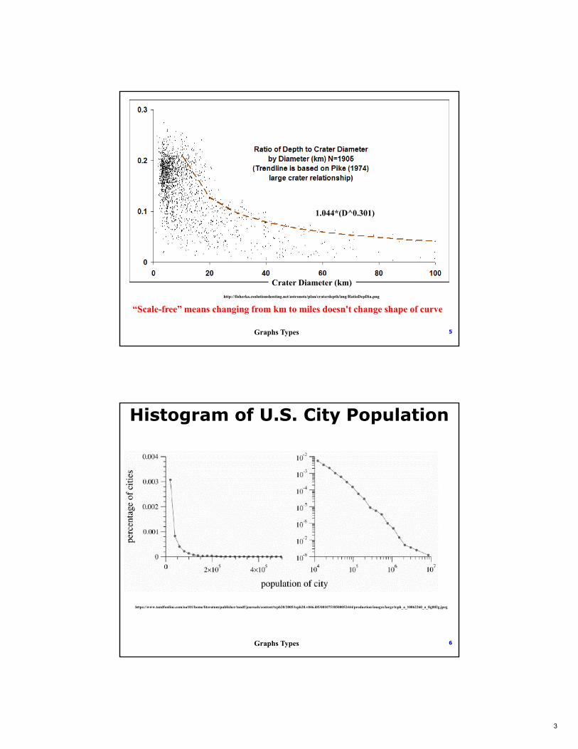
5Graphs Types

http://fisherka.csolutionshosting.net/astronote/plan/craterdepth/img/RatioDepDia.png

1.044*(D^0.301)

Crater Diameter (km)

“Scale-free” means changing from km to miles doesn't change shape of curve

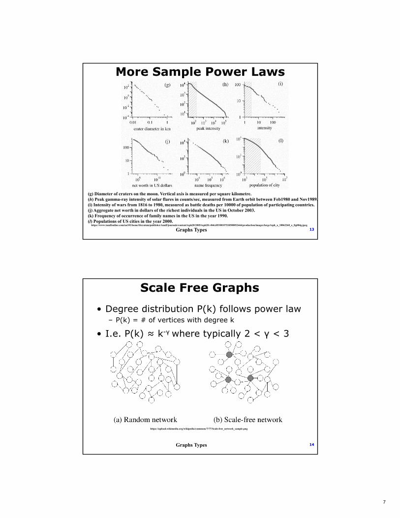
6Graphs Types

https://www.tandfonline.com/na101/home/literatum/publisher/tandf/journals/content/tcph20/2005/tcph20.v046.i05/00107510500052444/production/images/large/tcph_a_10062260_o_fig002g.jpeg

Histogram of U.S. City Population

4

7Graphs Types

Probability Density (Probability Mass)• function of a variable

– whose integral over any interval– is probability that variable will lie within that interval.

http://www.chrisbeales.net/env_images/env_dice%20probability%20graph.jpg

36 possible results from rolling 2 dice

8Graphs Types

https://cdn-images-1.medium.com/max/1600/1*IdGgdrY_n_9_YfkaCh-dag.png

μ = meanσ = std dev

# is integral of densityover interval

5

9Graphs Types

Power Law Distributions• If p(x) dx is prob. of some event having a

value from x to x+dx• Then if distribution is a power law• Then on log log curve it’s a straight line• Then log(p(x)) ≈ -γ*log(x) + c• or p(x) ≈ Cx-γ , C = ec

• These are distributions, thus -γ negative• Values on right-hand side are small

10Graphs Types

Cumulative Distributions of Power Law Distributions

• P(x>z) = ∫∞ p(x)• If p(x) = Cx-γ, then P(x>z) = (C/(γ-1))x(-γ+1)

• Again a straight line on log-log graph– But different slope

z

6

11Graphs Types

Looking for Power Laws in Real Data

• Notional approach– Compute histogram of data, with constant bin size– Graph on log-log curve– Measure slope & y-intercept

• Problem: – With constant bins, righthand cases have few events– Result: very “noisy”

• Better: use logarithmic binning:– Intervals get bigger when moving right– E.g. have intervals grow by some factor at each step

• Best: compute cumulative distribution and graph on log-log– Slope is -γ+1 rather than γ– https://www.tandfonline.com/doi/full/10.1080/00107510500052444?s

croll=top&needAccess=true

12Graphs Types

Sample Power Laws

https://www.tandfonline.com/na101/home/literatum/publisher/tandf/journals/content/tcph20/2005/tcph20.v046.i05/00107510500052444/production/images/large/tcph_a_10062260_o_fig004g.jpeg

(a) Numbers of occurrences of words in the novel Moby Dick by Hermann Melville. (b) Numbers of citations to scientific papers published in 1981, from time of publication until June 1997. (c) Numbers of hits on web sites by 60000 users of the America Online Internet service for the day of 1 December 1997.(d) Numbers of copies of bestselling books sold in the US between 1895 and 1965. (e) Number of calls received by AT&T telephone customers in the US for a single day. (f) Magnitude of earthquakes in California between January 1910 and May 1992. .

7

13Graphs Types

More Sample Power Laws

https://www.tandfonline.com/na101/home/literatum/publisher/tandf/journals/content/tcph20/2005/tcph20.v046.i05/00107510500052444/production/images/large/tcph_a_10062260_o_fig004g.jpeg

(g) Diameter of craters on the moon. Vertical axis is measured per square kilometre. (h) Peak gamma-ray intensity of solar flares in counts/sec, measured from Earth orbit between Feb1980 and Nov1989. (i) Intensity of wars from 1816 to 1980, measured as battle deaths per 10000 of population of participating countries.(j) Aggregate net worth in dollars of the richest individuals in the US in October 2003. (k) Frequency of occurrence of family names in the US in the year 1990. (l) Populations of US cities in the year 2000.

14Graphs Types

Scale Free Graphs• Degree distribution P(k) follows power law

– P(k) = # of vertices with degree k

• I.e. P(k) ≈ k-γ where typically 2 < γ < 3

https://upload.wikimedia.org/wikipedia/commons/7/77/Scale-free_network_sample.png

8

15Graphs Types

Erdős–Rényi Graph Model

• 1959• Goal: generate “Random Graphs”• Assumption: all graphs with fixed #

vertices and edges are equally likely• G(n, p) model:

– n vertices– Thus n(n-1)/2 possible edges– Probability of each edge being in a graph is p– Probability of any particular graph = pM(1-p) -=M

• Expected # edges is p

(n)2

16Graphs Types

Barabási–Albert Graph Model

• 1999• Generate scale-free power law graphs

using:– Assumption of Growth of # of vertices over time– Preferential Attachment: more connected a vertex

is, more likely to receive more edges

• Algorithm:– Assume initially m0 vertices– Add new vertices one at a time– Probability that new vertex connected to vertex v is– pv =kv/∑jkj, where kv is degree of v

• Resulting P(k) = k-3

9

17Graphs Types

Kronecker Graphs• Given real graph, generate a synthetic

graphs with matching properties• Algorithm: Build graph as adjacency matrix

– Start with initiator graph K1 with N1 vertices, E1 edges– Recursively build K2, K3, … where Kj has N1

j vertices – At each step take Kronecker product of Kj with itself

• Resulting graphs maintain many properties of original

18Graphs Types

Examples

https://cs.stanford.edu/~jure/pubs/kronecker-jmlr10.pdf

10

19Graphs Types

R-MAT Graph Generators• Used in Grap500 graph generation

– See D. Chakrabarti, Y. Zhan, and C. Faloutsos, R-MAT: A recursive model for graph mining, SIAM Data Mining 2004

• Algorithm: construct Adjacency Matrix– Recursively divide matrix into 4 submatrices

labelled a,b,c,d– Each submatrix has a probability– To add an edge, select source (and target)

vertex by• Use probabilities to select submatrix of full matrix• Use probabilities to select submatrix of submatrix• …• Stop on 1x1 submatrix

• To smooth out fluctuations in degree distribution, add some “noise” at each step

p(a) = 0.57p(b)=p(c) = 0.19p(d) = 0.05

20Graphs Types

Representing Sparse Adjacency Matrices

• Adjacency matrix for N vertex graph is N2

– One row/column per vertex– E.g. Graph500 graphs have 4 billion vertices– That’s 1.6x1019 elements

• Most real adjacency matrices VERY sparse– # of 1’s per row = degree of that vertex– Graph500 have on average 32 1’s per row

• Would rather not store O(N2) elements when all but O(N) are zero

11

21Graphs Types

Common Approaches• Dictionary of Keys

– Each non-zero recorded as (r,c,v) pair, in random order– Good for generating edge set dynamically– But slow when need to iterate

• E.g. step through edges leaving/arriving at some vertex

• Coordinate List:– Again (r,c,v) pairs but sorted first by row then by column– Improved random access time

• List of Lists:– One list per row, with (column, value) as element– Typically list is sorted by column number– Good for accessing by row, bad if by column

For adjacency matrices “value” = 1

22Graphs Types

Common Approaches• Compressed Sparse Row (CSR, CRS):

– Three 1D vectors• A: length NNZ (# of non-zeros) of values

– Listed in order of matching column index– Non needed for adjacency matrices where all values = 1

• AJ: length NNZ – column # for each non-zero• IA: length N+1 (N # of vertices) of indices into A

– IA[i] points to 1st non-zero for row I• IA[i+1]-IA[I]-1 = # of non-zeros for row I

– Fast access to individual rows of matrix– Slow access to columns– Expensive incremental adding of edges to graph

• Compressed Sparse Column(CSC, CCS)– Same as CSR but for columns rather than rows

12

23Graphs Types

Stinger

CSR but vectors in linked lists of blocks that hold several edges;• multiple edge types permitted• timestamps on edges• blocks may be on different nodes

IA

Etype vector has starting index to 1st block with edges of that type

Logical verticespermit relocating vertex data to different physical nodes

24Graphs Types

Compressed Vector Representation (CVR)

• Many microprocessors have “short vector” SIMD instructions– If values are in consecutive memory/registers– Then one “SIMD” instruction can perform lots of ops

• CVR reformats matrix so elements in consecutive order

• When doing SpMV-like need to create matching vectors

http://delivery.acm.org/10.1145/3170000/3168818/cgo18-p58.pdf?ip=129.74.153.250&id=3168818&acc=ACTIVE%20SERVICE&key=EA62C54EFA59E1BA%2E367AD4ADD93F5D2F%2E4D4702B0C3E38B35%2E4D4702B0C3E38B35&__acm__=1539193774_ecb3de8e8c575e521adc8a4447bf2240