grapevine age: impact on physiology and berry and wine quality
TRANSCRIPT
HAL Id: tel-02426245https://tel.archives-ouvertes.fr/tel-02426245
Submitted on 2 Jan 2020
HAL is a multi-disciplinary open accessarchive for the deposit and dissemination of sci-entific research documents, whether they are pub-lished or not. The documents may come fromteaching and research institutions in France orabroad, or from public or private research centers.
L’archive ouverte pluridisciplinaire HAL, estdestinée au dépôt et à la diffusion de documentsscientifiques de niveau recherche, publiés ou non,émanant des établissements d’enseignement et derecherche français ou étrangers, des laboratoirespublics ou privés.
Grapevine age : Impact on physiology and berry andwine qualityKhalil Bou Nader
To cite this version:Khalil Bou Nader. Grapevine age : Impact on physiology and berry and wine quality. Agricul-tural sciences. Université de Bordeaux; Hochschule Geisenheim University, 2018. English. �NNT :2018BORD0329�. �tel-02426245�

Grapevine Age:
Impact on Physiology and Berry and Wine Quality
Presented by
Khalil Bou Nader, MSc.
Thesis in co-supervision between
HOCHSCHULE GEISENHEIM UNIVERSITY
and
BORDEAUX UNIVERSITY
DOCTORAL SCHOOL OF LIFE AND HEALTH SCIENCES
to obtain a joint degree with the ranks of
DOCTOR OF AGRICULTURAL SCIENCES (Dr. agr.)
and
DOCTOR
Mention: Sciences, Technology, Health
Option: Enology
Defended on December 21, 2018
after a proper doctoral procedure in accordance with the provisions of the cooperation agreement "Convention de Cotutelle Internationale de Thèse entre l'Université Bordeaux et l’Université de Geisenheim" had been completed. Both doctoral degree certificates are only valid together and qualify for using either the German or French doctoral title.
Members of the jury:
Ms. Annette REINEKE Professor, Hochschule Geisenheim University President
Ms. Astrid FORNECK Professor, Universität für Bodenkultur Wien Reviewer
Mr. Laurent TORREGROSA Professor, Montpellier SupAgro Reviewer
Mr. Vivian ZUFFEREY Doctor, Institut de recherche Agroscope Reviewer
Mr. Manfred STOLL Professor, Hochschule Geisenheim University Thesis supervisor
Mr. Eric GOMÈS Professor, Université de Bordeaux Thesis supervisor


3
Declaration of authorship “I declare that I have prepared the submitted dissertation with the title
Grapevine Age: Impact on Physiology and Berry and Wine Quality
independently and without unauthorized third-party help and that no other than the in the dissertation
listed facilities have been used. All text passages that are quoted literally or analogously from other
published papers and all information that are based on verbal statements are identified as such. I have
observed the principles of good scientific practice as defined in the statutes of the HOCHSCHULE
GEISENHEIM UNIVERSITY and the UNIVERSITY OF BORDEAUX for safeguarding good
scientific practice when carrying out the analyses of my research mentioned in the dissertation.”
Place: Geisenheim Signature: Khalil Bou Nader
„Ich erkläre: Ich habe die vorgelegte Dissertation mit dem Titel
Grapevine Age: Impact on Physiology and Berry and Wine Quality
selbständig und ohne unerlaubte fremde Hilfe und nur mit den Hilfen angefertigt, die ich in der
Dissertation angegeben habe. Alle Textstellen, die wörtlich oder sinngemäß aus veröffentlichten
Schriften entnommen sind, und alle Angaben, die auf mündlichen Auskünften beruhen, sind als solche
kenntlich gemacht. Bei den von mir durchgeführten und in der Dissertation erwähnten Untersuchungen
habe ich die Grundsätze guter wissenschaftlicher Praxis, wie sie in den Satzungen der Hochschule
Geisenheim und der UNIVERSITY of BORDEAUX zur Sicherung guter wissenschaftlicher Praxis
niedergelegt sind, eingehalten.“
Ort: Geisenheim Unterschrift: Khalil Bou Nader
« Je declare avoir preparé la thèse soumise au titre
Grapevine Age: Impact on Physiology and Berry and Wine Quality
de manière indépendante et sans l'aide d'une tierce partie non autorisée et que seules les installations
mentionnées dans la thèse ont été utilisées. Tous les passages de texte cités littéralement ou de manière
analogue dans d'autres articles publiés et toutes les informations basées sur des déclarations verbales
sont identifiés comme tels. J'ai observé les principes de bonne pratique scientifique tels qu'ils sont
définis dans les statuts de l'UNIVERSITÉ HOCHSCHULE GEISENHEIM et de l'UNIVERSITÉ DE
BORDEAUX pour la sauvegarde de la bonne pratique scientifique lors de la réalisation des analyses
de mes recherches mentionnées dans la thèse. »
Lieu : Geisenheim Signature: Khalil Bou Nader

4
Acknowledgements
I would like to express my sincere gratitude and appreciation to the following people and staff:
- Profs. Manfred Stoll and Eric Gomès for their guidance and encouragements throughout
the PhD. It was a pleasure to work on this topic under their supervision.
- Prof. Hans-Reiner Schultz, Prof. Prof. Doris Rauhut, Dr. Claus-Dieter Patz, Prof. Rainer
Jung, and Prof. Otmar Löhnertz for their contributions to the project.
- Prof. Serge Delrot, Dr. Ghislaine Hilbert, Christel Renaud, and Dipl. Ing. Jean-Philippe
Roby for their support on the French side.
- Dipl. Ing Magali Blank, Dr. Susanne Tittmann, Annette Rheinberger, Sabrina Samer,
Regine Donecker, Jesus Felipe Ravelo Rodriguez, and Claude Bonnet for their help in the
laboratory.
- The members of various departments at HGU and the ISVV for the friendly and fruitful
collaboration that we maintained throughout the project.
- Elise Laizé Julian Dittmann, Liying Shao, Jakob Gasser, Maximilian Leonard Pfahl, and
Hélène Georges for their help with data collection.
- My PhD colleagues and other students in Geisenheim and Bordeaux, from whom I learned
a lot and whose company I always enjoyed.
Finally, I would like to extend my gratitude to my parents, my sisters and my friends for their
unconditional support. I would have never made it without you all, thank you!

“The first hundred years are the hardest.”
- Proverb -

6
Abstract
Vine age and its relation to the quality of the wine are topics of recurring interest, both scientific
and economic. Consumers and actors in the wine sector seem to agree on the ability of old vines to
produce wines of superior character. Despite ongoing research, the validity of this point of view
remains debated and questions about the mechanisms through which old vines would end up with
superior quality wines remain numerous. To try to answer them, the impact vine age on physiology,
tolerance to water stress, and berry and wine quality were studied in an experimental vineyard
planted with Vitis vinifera L. cv. of identical genetic material (Riesling Gm 239 grafted on 5C
Teleki) but planted in different years.
In 2014 and 2015, the vines planted in 2012 had not yet reached their full potential and had a
significantly lower vegetative productivity and yield than the vines planted in 1995 and 1971.
Moreover, the vines planted in 2012 were not subjected to the same grass treatment as older vines
during this period to prevent excessive competition during establishment. The lower capacity of
these vines and the absence of cover crop led to greater exposure of clusters to light and greater
nitrogen accumulation, which resulted in a higher concentration of amino acids, monoterpenes,
norisoprenoids, and flavonols in 2014 and 2015. In the following years (2016 and 2017), the yield
and pruning weight of these vines, as well as their berry composition, were comparable to those of
the older vines. The parameters of technological maturity (° Brix, total acidity and must pH) were
not significantly affected by vine age.
Vines planted in 1995 and 1971 showed similar physiological characteristics throughout the study
with the exception of a higher incidence of esca syndrome in the older group. This disease was
responsible for the decline in the total yield of vines planted in 1971, but individual yield per vine
was equivalent for both groups.
Sensory and chemical analyzes were conducted in 2017 on wines from previous vintages. The
wines of the youngest vines were associated with aromas of ripe fruit and the kerosene aroma that
is typical of Riesling. These wines were also identified by higher concentrations of potential
monoterpenes and norisoprenoids and volatile sulfur compounds in 2014 and 2015 only. The
sensory and chemical profiles of wines from vineyards planted in 1995 and 1971 were dependent
on the vintage but not on the age of the vines. The wine profiles produced in 2016 were overlapping
for the three age groups.

7
The works described in this thesis manuscript are unique, particularly because the vineyard in
which they were conducted was designed specifically to study the effect of the age of the vine
under comparable environmental conditions. Once the youngest vines reached their fruiting
potential and were conducted in the same way as the older vines, their productivity, the composition
of their berries and the quality of the wines they produce converged with those of the two other
groups. More interestingly, vines aged 19 and 43 years behaved similarly throughout the study and
resulted in wines comparable in terms of sensory analysis, which goes against the an idea that the
older vines produce wines of a different profile.
Previous studies have shown that the productivity of the vines, whatever their age, could be
explained by the wood reserves and the size of the trunk. To have a better idea of differences linked
to reserves, the structure-from-motion with multi-view stereo-photogrammetry (SfM-MVS)
method was tested to measure trunk thickness and volume. The technique, which allows the
creation of scaled, georeferenced 3D models based on photographs, was able to produce accurate
models of field-grown grapevine trunks.
Keywords: old vine, water deficit, berry composition, wine quality, sensory analysis.
Zusammenfassung
Das Rebalter und seine Beziehung zur Weinqualität sind Themen von wiederkehrendem Interesse,
sowohl wissenschaftlich als auch wirtschaftlich. Vielfach wird behauptet, dass alte Reben Weine
mit besonderem Charakter produzieren können. Trotz vielfältiger Forschung bleibt diese
Sichtweise jedoch nicht eindeutig belegt, und es gibt immer noch mehr offene Fragen als erklärende
Antworten. Deshalb wurde auf einer Rebfläche der Hochschule Geisenheim University hierzu über
viele Jahre eine einzigartige Versuchsfläche aufgebaut. Dort ist es möglich, Untersuchungen
innerhalb einer Rebfläche (Geisenheimer Fuchsberg) für eine Rebsorte (Riesling) gleichen Klons
(Gm 239), gleicher Unterlage (5C Teleki) und auf einheitlichem Standraum (2,8 m2) an Reben der
drei Pflanzjahre 1971 („alt“), 1995 („alternd“) und 2012 („jung“) durchzuführen. Über einen
Zeitraum von vier Vegetationsperioden wurden verschiedene Fragen bearbeitet.
In den Versuchsjahren 2014 und 2015 hatten die im Jahr 2012 gepflanzten Reben noch nicht ihr
volles Ertragspotenzial erreicht und zeigten eine deutlich geringere vegetative Produktivität als die
in den Jahren 1995 und 1971 gepflanzten Reben. In diesen Anfangsjahren unterschied sich die

8
Bodenbewirtschaftung zwischen den drei Versuchsgliedern durch offene Bodenbewirtschaftung
oder eine Dauerbegrünung. Die geringere Wüchsigkeit der jungen Reben und die höhere
Mineralisationsrate der offenen Böden führten zu einer stärkeren Exposition der Trauben und einer
stärkeren Anreicherung von hefeverwertbarem Stickstoff, Aminosäuren, Monoterpenen,
Norisoprenoiden und Flavonolen in den Jahren 2014 und 2015. In den folgenden Jahren (2016 und
2017) waren Ertrag und Schnittholzgewicht der jungen Reben sowie deren
Beerenzusammensetzung mit denen der älteren Rebstöcke vergleichbar. Die Parameter der
technologischen Reife (° Brix, Gesamtsäure- und pH-Wert) wurden durch das Alter der Rebe nicht
wesentlich beeinflusst.
Die in den Jahren 1995 und 1971 gepflanzten Reben zeigten in der gesamten Studie ähnliche
physiologische Merkmale mit Ausnahme eines häufigeren Auftretens von Esca-Symptomen bei
den älteren Reben. Diese Krankheit war für den Rückgang des Gesamtertrags der im Jahr 1971
gepflanzten Rebstöcke verantwortlich, wobei hervorzuheben ist, dass der Einzelstockertrag aller
drei Versuchsglieder dann auch gleich war.
Im Jahr 2017 wurden sensorische und chemische Analysen der Weine aus früheren Jahrgängen
durchgeführt. Die Geschmacksattribute der Weine der jungen Reben wurden mit Aromen von
reifen Früchten und dem für Riesling typischen Kerosinaroma in Verbindung gebracht. In diesen
Weinen wurden auch in den Jahren 2014 und 2015 höhere Konzentrationen potenzieller
Monoterpene und Norisoprenoide sowie flüchtiger Schwefelverbindungen festgestellt. Die
sensorischen Profile der Weine aller Versuchsjahre und des Rebalters waren stärker vom
Weinjahrgang selbst als vom Alter der Reben geprägt. Sobald die jungen Reben das
Ertragspotential erreicht hatten und auf dieselbe Weise wie die älteren Reben bewirtschaftet
wurden, stimmten ihre Produktivität, die Zusammensetzung ihrer Beeren und die Qualität der
Weine mit denen der beiden anderen Versuchsglieder überein. Interessanterweise traten zwischen
den 1971 und 1995 gepflanzten Reben bei physiologischen Messungen und sensorischen
Untersuchungen keine Unterschiede auf.
Frühere Studien haben einen Zusammenhang zwischen der Produktivität der Reben und der
Reservestoffe im Holz gezeigt. Hierzu wurde im Rahmen der eigenen Untersuchungen mittels der
„structure-from-motion with multi-view stereo-photogrammetry“ (SfM-MVS) das Stammvolumen
untersucht und erstmals ein 3-D-Modell des Rebstammes publiziert.
Schlagworte: alte Reben, Wasserstress, Traubeninhaltsstoffe, Weinqualität, sensorische Prüfung.

9
Résumé
L’âge de la vigne et sa relation avec la qualité du vin sont des sujets d’intérêt récurrents, tant
scientifiques qu’économiques. Les consommateurs et acteurs de la filière vitivinicole semblent
s’accorder à propos de la capacité des vieilles vignes à produire des vins de caractère supérieur.
Malgré les recherches en cours, la validité de ce point de vue reste débattue et les questions
concernant les mécanismes à travers lesquels de vieilles vignes aboutiraient à des vins qualité
supérieure restent nombreuses. Pour tenter d’y répondre, l’impact de l’âge des vignes sur la
physiologie, la tolérance au stress hydrique, ainsi que la qualité des baies et du vin ont été étudiés
dans un vignoble expérimental constitué de plants de Vitis vinifera L. cv. de matétiel génétique
identique (Riesling de clone Gm 239 greffé sur 5C Teleki) mais aux dates de plantation différentes.
En 2014 et 2015, les vignes plantées en 2012 n’avaient pas encore atteint leur plein potentiel et
avaient une productivité végétative et un rendement significativement inférieurs à ceux des vignes
plantées en 1995 et 1971. Par ailleurs, les vignes plantées en 2012 n’ont pas été soumises au même
traitement d’enherbement que les vignes plus âgées pendant cette période afin de prévenir une
compétition excessive pendant leur établissement. La capacité inférieure de ces vignes et l’absence
d’enherbement ont mené à une plus grande exposition des grappes à la lumière et une plus grande
accumulation d’azote, ce qui s’est traduit par une plus grande concentration en acides aminés,
monoterpènes, norisoprénoides, et flavonols en 2014 et 2015. Les années suivantes (2016 et 2017),
le rendement et le poids des bois de taille de ces vignes, ainsi que la composition des baies, étaient
comparables à ceux des vignes plus âgées. Les paramètres de maturité technologique (°Brix,
l’acidité totale et le pH de moûts) n’ont pas été significativement affectés par l’âge des vignes.
Les vignes plantées en 1995 et 1971 ont présenté des caractéristiques physiologiques similaires
tout au long de l’étude à l’exception d’une plus grande incidence du syndrome de l’esca chez le
groupe le plus âgé. Cette maladie a été responsable de la baisse du rendement à la parcelle des
vignes plantées en 1971, les rendements individuels à l’échelle du cep restant équivalents pour les
deux groupes.
Des analyses sensorielles et chimiques ont été réalisées en 2017 sur des vins de millésimes
précédents. Les vins des plus jeunes vignes ont été associés à des arômes de fruits mûrs et de
l’arôme de pétrole typique du Riesling. Ces vins ont aussi été identifiés par de plus hautes
concentrations de monoterpènes et norisoprénoides potentiels et de composés soufrés volatils, en

10
2014 et 2015 uniquement. Les profils sensoriels et chimiques de vins issus des vignes plantées en
1995 et 1971 étaient dépendants du millésime mais pas de l’âge des vignes. Les profils des vins
produits en 2016 étaient en superposables pour les trois groupes d’âge.
Les travaux décrit dans ce manuscrit de thèse sont uniques, du fait notamment que le vignoble dans
lequel ils ont été conduits a été conçu spécifiquement pour étudier l’effet de l’âge de la vigne dans
des conditions environnementales comparables. Une fois que les vignes les plus jeunes ont atteint
leur potentiel fructifère et ont été conduites de la même manière que les vignes plus âgées, leur
productivité, la composition de leurs baies et la qualité des vins qu’elles produisent ont convergé
avec celles des deux autres groupes. Plus intéressant encore, des vignes âgées de 19 et 43 ans se
sont comportées de la même façon tout au long de l’étude et ont abouti à des vins comparables en
termes d’analyses sensorielles, ce qui va à l’encontre de l’idée reçue qui veut que les vignes les
plus âgées produisent des vins de qualité différente.
Des travaux précédents ont démontré que la productivité des vignes, quel que soit leur âge, pouvait
être expliquée par les réserves de bois et par la taille du tronc. Pour avoir une meilleure idée des
différences liées aux réserves, la technique dite « structure-from-motion with multi-view stereo-
photogrammetry » (SfM-MVS) a été testée pour mesurer l’épaisseur des troncs et leur volume.
Cette technique qui permet la création de modèles tridimensionnels géo-référencés et à l’échelle a
pu générer des modèles précis de tronc de vignes plantées en champ.
Mots-clés : vieille vigne, déficit hydrique, composition de la baie, qualité du vin, analyse
sensorielle.

11
Table of contents
Declaration of authorship ................................................................................................................. 3
Acknowledgements .......................................................................................................................... 4
Abstract ............................................................................................................................................ 6
Zusammenfassung ............................................................................................................................ 7
Résumé ............................................................................................................................................. 9
Table of contents ............................................................................................................................ 11
List of tables ................................................................................................................................... 14
List of figures ................................................................................................................................. 16
List of appendices .......................................................................................................................... 19
List of abbreviations ....................................................................................................................... 21
Chapter 1. General Introduction ..................................................................................................... 24
1. Wine quality and grapevine age ....................................................................................... 26
1.1. The dimensions of wine quality ............................................................................... 26
1.2. A bottle of old vines ................................................................................................. 27
1.3. Grapevine age and wine quality in the scientific literature ...................................... 29
2. Grapevine vigor and balance ........................................................................................... 32
2.1. Factors influencing grapevine vigor......................................................................... 32
2.2. Consequences of excessive vigor ............................................................................. 38
2.3. Achieving grapevine balance ................................................................................... 41
3. Grapevine water relations ................................................................................................ 45
3.1. Cellular and physiological water transport mechanisms .......................................... 45
3.2. Grapevine responses to water deficit ....................................................................... 46
4. Berry development and composition ............................................................................... 48
4.1. Berry structure .......................................................................................................... 48
4.2. Berry development ................................................................................................... 49
5. The Riesling cultivar ........................................................................................................ 51
5.1. Varietal aromas of Riesling ...................................................................................... 52
6. Objectives of the thesis .................................................................................................... 55
Chapter 2. Impact of grapevine age on water status and productivity ........................................... 56
1. Abstract ............................................................................................................................ 57
2. Introduction ...................................................................................................................... 57
3. Materials and methods ..................................................................................................... 59

12
3.1. Weather data............................................................................................................. 59
3.2. Experimental design and plant material ................................................................... 59
3.3. Gas exchange measurements.................................................................................... 61
3.4. Vine capacity and balance ........................................................................................ 61
3.5. Berry technological maturity and δ13C..................................................................... 62
3.6. Experiment on water deficit ..................................................................................... 63
3.7. Statistical analysis .................................................................................................... 63
4. Results .............................................................................................................................. 64
4.1. Weather data............................................................................................................. 64
4.2. Vine selection and soil management ........................................................................ 65
4.3. Gas exchange measurements.................................................................................... 68
4.4. Vine capacity and balance ........................................................................................ 69
4.5. Berry technological maturity and δ13C ................................................................... 74
4.6. Experiment on water deficit ..................................................................................... 74
5. Discussion ........................................................................................................................ 78
6. Conclusion ....................................................................................................................... 82
7. Acknowledgments ............................................................................................................ 83
8. Funding ............................................................................................................................ 83
Chapter 3. Impact of grapevine age on berry structure and secondary metabolites ...................... 84
1. Introduction ...................................................................................................................... 85
2. Materials and methods ..................................................................................................... 86
2.1. Experimental design and plant material ................................................................... 86
2.2. Berry sampling ......................................................................................................... 87
2.3. Organic and amino acids .......................................................................................... 88
2.4. Potentially volatile monoterpenes and C13-norisoprenoids ...................................... 89
2.5. Flavonol content in berry skin ................................................................................. 90
2.6. Statistical analysis .................................................................................................... 91
3. Results and discussion ..................................................................................................... 91
3.1. Berry composition .................................................................................................... 91
3.2. Secondary metabolites and light interception .......................................................... 97
4. Conclusion ....................................................................................................................... 98
Chapter 4. Impact of grapevine age on wine composition and sensory attributes ....................... 100
1. Introduction .................................................................................................................... 101
2. Materials and methods ................................................................................................... 102

13
2.1. Experimental design and plant material ................................................................. 102
2.2. Winemaking ........................................................................................................... 103
2.3. Sensory analysis ..................................................................................................... 103
2.4. Wine composition .................................................................................................. 105
2.5. Statistical analysis .................................................................................................. 108
3. Results and discussion ................................................................................................... 109
3.1. Sensory analysis ..................................................................................................... 109
3.2. Chemical analysis................................................................................................... 112
3.3. MFA with chemical and sensory data .................................................................... 113
3.4. PCA of chemical data for older wines ................................................................... 116
4. Conclusion ..................................................................................................................... 117
Chapter 5. Evaluating grapevine trunk size with a handheld camera by 3D modeling ............... 118
1. Abstract .......................................................................................................................... 119
2. Introduction .................................................................................................................... 119
3. Materials and methods ................................................................................................... 121
3.1. Plant material and field-measured trunk diameter and circumference ................... 121
3.2. Image acquisition for trunk reconstruction ............................................................ 122
3.3. 3D model reconstruction by SfM-MVS ................................................................. 123
3.4. SfM-MVS measurements and model validation .................................................... 124
3.5. Estimation of trunk volume and crown contribution ............................................. 124
3.6. Statistical analysis .................................................................................................. 125
4. Results and discussion ................................................................................................... 126
4.1. SfM-MVS measurements and model validation .................................................... 126
4.2. Exclusion of the grapevine crown .......................................................................... 128
5. Conclusion ..................................................................................................................... 129
Chapter 6. General discussion ...................................................................................................... 130
Appendices ................................................................................................................................... 137
References .................................................................................................................................... 158

14
List of tables
Table 1.1. Overview of the current literature related to grapevine age. The grapevine age column refers
to the youngest and oldest grapevines in their respective study (adapted from Grigg et al., 2017).
........................................................................................................................................................ 31
Table 1.2. Optimal ranges for various grapevine balance indices aggregated from various studies
(adapted from Dry et al., 2004). ..................................................................................................... 42
Table 1.3. Top five countries by Riesling vineyard area in 2015 (data sourced from OIV, 2018b, 2017).
........................................................................................................................................................ 52
Table 2.1. Growing degree-day (GDD) and precipitation data for Geisenheim Fuchsberg, Germany,
from April 1st to October 31st for the growing seasons 2014-2017. The yearly average represents
the period of 1981-2010. ................................................................................................................ 64
Table 2.2. Percentages among vines planted in 1971 and 1995 of healthy vines, vines with esca
symptoms, and missing vines as visually assessed at the end of each growing season between 2015
and 2017. ........................................................................................................................................ 70
Table 2.3. Vine balance parameters for three age groups and four replicates over the growing seasons
2014-2017 (n = 4). Fruit yield (which includes rotten berries) and pruning weight refer to values
recorded in the field, while adjusted fruit yield and pruning weight take into account the number of
missing vines per row (means ± sd). .............................................................................................. 73
Table 2.4. Technological maturity parameters and dry mass carbon isotope discrimination (δ13C) for
the three grapevine age groups (n = 4) over the growing seasons 2014 to 2017 (means ± sd). δ13C
was only measured in 2016 and 2017. ........................................................................................... 74
Table 3.1. Maturity pqrameters and amino acid concentrations for the three grapevine age groups (n
= 4) over the growing seasons 2015 to 2017. ................................................................................ 93
Table 3.2. Free and potentially volatile monoterpenes and norisoprenoids, and flavonol glycosidesfor
the three grqpevine qge groups (n = 4) from 2015 to 2017. .......................................................... 94
Table 4.1. Composition of aroma reference standards prepared using aroma standards by soaking in
propanediol (Pd). .......................................................................................................................... 105
Table 4.2. Taste reference standards with low and high concentrations. ......................................... 105
Table 4.3. Average ratings per attribute in the 2017 tasting for wines from the three grapevine age
groups (vintages 2014 to 2016). The means and standard deviations were calculated from three
replications with 12 panelists. ...................................................................................................... 111

15
Table 4.4. List of the compounds analyzed in wine. ........................................................................ 113
Table 5.1. Overview of the three grapevine ages used in the 2017 study on trunk size. .................. 121
Table 5.2. Field-measured and modeled metrics for 5-year-old, 22-year-old, and 46-year-old
grapevines (presented as mean ± sandard deviation) and the root mean square error (RMSE) and
bias of modelled data. .................................................................................................................. 127
Table 5.3. Comparison between total trunk volume and trunk volume 40 cm above the grafting point
and the volume fraction formed by the grapevine crown (data presented as mean ± standard
deviation)...................................................................................................................................... 128

16
List of figures
Figure 1.1. In the center, the 'Old Vine' of Maribor, Slovenia (Bogdan Zelnik, www.maribor-pohorje.si.
Accessed October 2018). ............................................................................................................... 27
Figure 1.2. 'Vegetative' cycle during which shade stimulates vegetative growth at the expense of yield
and quality. (b) 'Balanced' cycle where light favors shoot fruitfulness, leading to balance between
shoot and fruit growth (adapted from Smart and Robinson, 1991)................................................ 39
Figure 1.3. Schematic model of steady water flow through a plant, from soil to atmosphere. Water
uptake at the roots, long-distance transport in the xylem and stomatal resistances are represented
as resistors of relative resistance placed in series (Reproduced from Steudle 2000b). .................. 47
Figure 1.4. Schematic representation of the grape berry at maturity (reproduced from Coombe, 1987).
........................................................................................................................................................ 49
Figure 1.5. Diagram showing the double sigmoid growth curve of berry development, including the
timing of accumulation of metabolites and indications of xylem and phloem inflow rates
(reproduced from Kennedy, 2002). ................................................................................................ 50
Figure 2.1. Double Guyot vine selection process in 2014 with trunk diameter and fruitful bud count
for all vines and for the 24 selected vines per age group. .............................................................. 65
Figure 2.2. Fruitful bud count of selected double Guyot vines from 2014 to 2017 (n = 24). ............. 66
Figure 2.3. Soil nitrate content measured at horizons 0-30 cm and 30-60 cm over the growing seasons
2014-2017 for double Guyot rows planted in 1971, 1995, and 2012 (means ± sd). ...................... 67
Figure 2.4. Soil water content measured at horizons 0-30 cm and 30-60 cm over the growing seasons
2014-2017 for double Guyot rows planted in 1971, 1995, and 2012 (means ± sd). ...................... 67
Figure 2.5. Chlorophyll fluorescence ratio under green excitation (SFR_G) measured at regular time
intervals on selected double Guyot vines from flowering to harvest over the growing seasons 2014-
2017 (means ± sd). ......................................................................................................................... 68
Figure 2.6. Leaf assimilation (AN), stomatal conductance (gs), and transpiration (E) measured
periodically on double Guyot vines over the growing seasons 2016 and 2017 with n = 24 (means ±
sd). .................................................................................................................................................. 69
Figure 2.7. PCA biplot of point quadrat analysis, cluster architecture and grapevine balance
components for 2014-2016. The point labels represent the growing season followed by the
grapevine age group (‘O’ for old grapevines planted in 1971; ‘M’ for ‘mature’ grapevines planted
in 1995; ‘Y’ for ‘young’ grapevines planted in 2012). There are four replicates per growing season
per age group. They are represented by the numbers 1 to 4 next to the letter. .............................. 72
17
Figure 2.8. Soil water content for the water deficit experiment on cordon vines in 2016 and 2017 at
flowering, pea-sized berries, and two weeks after veraison (means ± sd) at horizons 0-30 cm and
30-60 cm. ....................................................................................................................................... 76
Figure 2.9. Chlorophyll fluorescence ratio under green excitation (SFR_G) measured at regular time
intervals on selected cordon vines for the water deficit experiment from flowering to harvest in
2016 and 2017 (means ± sd). ......................................................................................................... 76
Figure 2.10. Stomatal conductance (gs) measured periodically on selected cordon vines for the water
deficit experiment over the growing seasons of 2016 and 2017 (means ± sd). ............................. 77
Figure 2.11. Predawn water potential (ΨPD) measured on cordon-trained vines for the water deficit
experiment over the growing seasons of 2016 and 2017 (means ± sd). ........................................ 77
Figure 3.1. PCA score plot of technological parameters and secondary metabolites (amino acids,
quercetin glucosides, and free and potentially volatile terpenes and norisoprenoids) from 2015-
2017. The point labels represent the growing season followed by the grapevine age group (‘O’ for
‘old’ grapevines planted in 1971; ‘M’ for ‘mature’ grapevines planted in 1995; ‘Y’ for ‘young’
grapevines planted in 2012). There are four replicates per growing season per age group,
represented by the numbers 1 to 4 next to the letter. ..................................................................... 95
Figure 3.2. Loadings plot of technological parameters and secondary metabolites (amino acids,
quercetin glucosides, and free and potentially volatile terpenes and norisoprenoids) from 2015-
2017. ............................................................................................................................................... 95
Figure 3.3. k-means clustering of the technological parameters and secondary metabolites, with four
clusters and 50 iterations. The centroid positions were calculated as to minimize the sum of squares
within each cluster. The point labels represent the growing season followed by the grapevine age
group (‘O’ for ‘old’ grapevines planted in 1971; ‘M’ for ‘mature’ grapevines planted in 1995; ‘Y’
for ‘young’ grapevines planted in 2012). There are four replicates per growing season per age group.
They are represented by the numbers 1 to 4 next to the letter. ...................................................... 96
Figure 3.4. PCA biplot of bound and free terpenes and quercetin glucosides in berry must at harvest
from 2015 to 2017. The point labels represent the growing season followed by the grapevine age
group (‘O’ for ‘old’ grapevines planted in 1971; ‘M’ for ‘mature’ grapevines planted in 1995; ‘Y’
for ‘young’ grapevines planted in 2012). There are four replicates per growing season per age group.
They are represented by the numbers 1 to 4 next to the letter. ...................................................... 98
Figure 4.1. PCA biplot of the 2017 sensory analysis of grapevines from the three grapevine age groups.
The point labels represent the growing season followed by the grapevine age group (‘O’ for ‘old’
grapevines planted in 1971; ‘M’ for ‘mature’ grapevines planted in 1995; ‘Y’ for ‘young’
grapevines planted in 2012). There are four replicates per growing season per age group,
represented by the numbers 1 to 4 next to the letter. ................................................................... 112

18
Figure 4.2. MFA Loadings plot of the sensory and chemical and sensory variables analyzed in 2017.
...................................................................................................................................................... 115
Figure 4.3. MFA partial score plot with chemical sensory variables analyzed in 2017. The point labels
represent the growing season followed by the grapevine age group (‘O’ for ‘old’ grapevines planted
in 1971; ‘M’ for ‘mature’ grapevines planted in 1995; ‘Y’ for ‘young’ grapevines planted in 2012).
There are four replicates per growing season per age group, represented by the numbers 1 to 4 next
to the letter.................................................................................................................................... 115
Figure 4.4. PCA score plot from the chemical analysis of wines from 2002 to 2016. Some vintages
were not available for analysis. The point labels represent the growing season followed by the
grapevine age group (‘O’ for ‘old’ grapevines planted in 1971; ‘M’ for ‘mature’ grapevines planted
in 1995; ‘Y’ for ‘young’ grapevines planted in 2012). There are four replicates per growing season
per age group, represented by the numbers 1 to 4 next to the letter. ........................................... 116
Figure 4.5. PCA loadings plot from the chemical analysis of wines from 2002 to 2016. ................ 117
Figure 5.1. Example of the experimental setup for taking the pictures (a) with a general view of
grapevine with the georeference grid and the point of measurement (white arrow); (b) focus on the
point of measurement of trunk circumference and cross-sectional area 10 cm above the grafting
point highlighted in the field using a plastic cord; (c) focus on the georeference grid around the
base of the trunk. .......................................................................................................................... 122
Figure 5.2. Images of the SfM-MVS reconstructed grapevine a) with squares representing camera
positions when taking photographs; b) showing the intact trunk (left), the trunk cross-section 10
cm above the grafting point with the two orthogonal diameters (middle), and the modeled disc
(right)............................................................................................................................................ 123
Figure 5.3. (a) Example of a complex crown on a 46 year old vine; (b) removal of the crown by
truncating the trunk volume to 40 cm above the grafting point. .................................................. 125
Figure 5.4. Regression analysis of the trunk diameter in the row direction (drow) and in the direction
perpendicular to the row (dper), the trunk cross-sectional area (TCSA), and the trunk circumference
with SfM-MVS estimates against field values for grapevines aged aged 5 (), 22 (), and 46 years
(). .............................................................................................................................................. 126
19
List of appendices
Appendix 2.1. Images of the plastic covers when retracted and deployed (approximate surface of 20
m2) around the four vines with the “stress” treatment. ................................................................ 137
Appendix 2.2. Daily mean temperatures, precipitations, and main phenological stages for the years
2014-2017. The black line represents the global average of daily temperatures from 1981 to 2010.
...................................................................................................................................................... 138
Appendix 2.3. LMM results for double Guyot including soil NO3- and water contents from 0-30 cm
and 30-60 cm (n = 4), leaf chlorophyll index, assimilation, stomatal conductance, transpiration (n
= 24), and carbon isotope discrimination (n = 4). The data represents three age groups and four
replicates over the growing seasons 2014-2017. Three measurements were made for soil NO3- and
water contents per vintage (flowering, veraison, and harvest), while six measures were taken
between 400 GDD and harvest for the chlorophyll index depending on weather conditions.
Assimilation, stomatal conductance and transpiration measured four times during the season. . 139
Appendix 2.4. Leaf chlorophyll index (SFR_G) for selected vines planted in 1971 (a) and 2012 (b)
from 2014 to 2017. The red points represent the vines R#61-15 and R#56b-2, which were found to
be positive for GLRaV-1 (grapevine leafroll-associated virus 1) and GFLV (grapevine fan-leaf
virus) respectively. ....................................................................................................................... 140
Appendix 2.5. LMM results for double Guyot vine balance parameters for three age groups and four
replicates over the growing seasons 2014-2017 (n = 4). .............................................................. 141
Appendix 2.6. LMM results for double Guyot vine balance parameters for vines planted in 1995 and
1971 with four replicates over the growing seasons 2014-2017 (n = 4). .................................... 143
Appendix 2.7. Eigen values and Eigen vectors from principal component analysis presented in Figure
2.7. ................................................................................................................................................ 144
Appendix 2.8. LMM results for double Guyot berry technological maturity for the three age groups
and four replicates over the growing seasons 2014-2017 (n = 4). ............................................... 145
Appendix 2.9. LMM results for the water deficit trial on cordon vines. Soil water content from 0-30
cm and 30-60 cm (n = 4), leaf chlorophyll index (n = 8), stomatal conductance (n = 8), predawn
water potential (n = 8), and carbon isotope discrimination (n = 4). The data represents three age
groups, two water deficit treatments, and four replicates over the growing seasons 2016-2017.
Three measurements were made for soil water content per vintage (flowering, pea size, and two
weeks after veraison). Six measures were taken between 400 GDD and harvest for chlorophyll
index and stomatal conductance in 2016 and seven measures in 2017, depending on weather
conditions. Four measures were taken for predawn water potential during the same period. Carbon
isotope discrimination was measured on berry samples at harvest. ............................................. 146

20
Appendix 3.1. Eigenvalues and eigenvectors from principal component analysis presented in Figure
3.2. ................................................................................................................................................ 148
Appendix 3.2. Mean values per cluster from the k-mean clustering in Figure 3.3. .......................... 149
Appendix 3.3. Eigenvalues and eigenvectors from principal component analysis presented in Figure
3.4. ................................................................................................................................................ 150
Appendix 4.1. ANOVA P-values from the sensory descriptive analysis in 2017. ........................... 151
Appendix 4.2. Eigenvalues and eigenvectors from principal component analysis presented in Figure
4.1 ................................................................................................................................................. 151
Appendix 4.3. Concentrations of free qnd potentially volatile monoterpenes qnd norisoprenoids
(μg L- 1) measured in available wines from 2002 to 2016. .......................................................... 152
Appendix 4.4. Volatile sulfur compounds (µg L-1) measured in available wines from 2002 to 2016.
Only H2S and DMS were detected in wine. ................................................................................. 153
Appendix 4.5. Chemical compounds by 1H NMR and CIELab parameters measured in available wines
from 2002 to 2016. ....................................................................................................................... 154
Appendix 4.6. Organic acids measured by HPLC (g L-1) in available wines from 2002 to 2016. ... 155
Appendix 4.7. Eigenvalues and eigenvectors from principal component analysis presented in Figure
4.2. ................................................................................................................................................ 156
Appendix 4.8. Eigenvalues and eigenvectors from principal component analysis presented in Figure
4.4. ................................................................................................................................................ 157

List of abbreviations
°Brix °Brix
3SH 3-sulfanylhexan-1-ol
4MSP 4-methyl-4-sulfanylpentan-2-one
a* Red/green
ABA Abscisic acid
AN Leaf assimilation
ArMV Arabis Mosaic Virus
B Boron
b* Yellow/blue
Ca Calcium
Cl- Chlorine
CS2 Carbon disulfide
Cu Copper
D2O Deuterium oxide
DA Descriptive analysis
DEDS Diethyl disulfide
DI Deficit irrigation
DMAPP Dimethyl allyl diphosphate
DMDS Dimethyl disulfide
DMH Octan-3-ol and 2.6-dimethylhept-5-en-2-ol
DMS Dimethyl sulfide
DMTS Dimethyl trisulfide
dper Trunk diameter in the direction perpendicular to the row
drow Trunk diameter in the row direction
E Transpiration
EDTA Ethylenediamine tetra acetic acid
EGFV Ecophysiology and Functional Genomics
EI Electron impact mode
ELISA Enzyme-Linked Immunosorbent Assay
EtSAc Thioaceticacid -S- ethyl ester
EtSH Ethanethiol
Fe Iron
GC-MS Gas chromatography coupled with mass spectrometry
GDC Geneva double curtain
GDD Growing degree-day
GFkV Grapevine Fleck Virus
GFlV Grapevine Flanleaf Virus
GLRaV-1 Grapevine Leafroll-Associated Virus 1

0 - List of abbreviations |
22
GLRaV-3 Grapevine Leafroll-Associated Virus 3
GPP Geranyl phosphate
gs Stomatal conductance
H2S Hydrogen sulfide
HCA Hierarchical cluster analysis
HCl Hydrochloric acid
HGU Hochschule Geisenheim University
IPP Isopentenyl pyrophosphate
ISVV Institute of grapevine and Wine Sciences
K Potassium
K2PO4 Dipotassium phosphate
K2S2O5 Potassium metabisulfite
L* Lightness
LA/Y Leaf area to fruit yield ratio
LC-MS Liquid chromatography coupled with mass spectrometry
LLN Leaf layer number
LMM Linear mixed-effect models
MeSAc Thioaceticacid -S- methyl ester
MeSH Methanethiol (MeSH)
MFA Multiple factor analysis
Mg Magnesium
MPa Megapascal
N Nitrogen
NH4+ Ammonium
NMR Nuclear magnetic resonance
NO3- Nitrate
P Phosphorus
PAR Photosynthetically active radiation
PC Principal component
PCA Principal component analysis
Pd Propanediol
PG Percent gaps
PHPD Pulsed flame photometric detector
PIC Percentage interior clusters
PIL Percent interior leaves
PRD Partial rootzone drying
RDI Regulated deficit irrigation
REML Restricted maximum likelihood
rh Relative humidity
RMSE Root mean square error
S Sulfur
S/N Signal-to-noise ratio

0 - List of abbreviations |
23
SD Standard deviation
SfM-MVS Structure-from-motion with multi-view stereo-photogrammetry
SFR_G Chlorophyll fluorescence ratio under green excitation
SIM Selected ion monitoring mode
SO2 Sulfur dioxide
SO32- Sulfite ion
SO42- Sulfate ion
SPE Solid-phase extraction
SW Sweep width
SWC Soil water content
SWHC Soil water holding capacity
TA Total acidity
TCSA Trunk cross-sectional area
TDN 1,1,6-trimethyl-1,2-dihydronaphtalene
TSP 3-(trimethylsilyl)propanoic acid sodium salt
TSS Total soluble solid
UHPLC Ultra-high performance liquid chromatography
UTCC Under-trellis cover crop
VPD Vapor pressure deficit
VSC Volatile sulfur compounds
VvDXS Deoxy-D-xylulose synthase
VvTS Vitis vinifera
WUE Water use efficiency
Y/P Yield to pruning weight ratio
YAN Yeast-assimilable nitrogen
δ13C Dry mass carbon isotope discrimination
Ψ Water potential
ΨM Surface tension forces
ΨPD Predawn water potential
Ψsoil Soil water potential
Ψπ Osmotic potential

Chapter 1 - General Introduction |
24
Chapter 1. General Introduction
“The trick is growing up without growing old.”
- Casey Stengel -

Chapter 1 - General Introduction |
25
Wine is a unique commodity that has been produced even before history was recorded (Bisson
et al., 2002; McGovern, 2013). As noted by Phillips (2000), “it is perhaps the most historically
charged and culturally symbolic of the foods and beverages with which we regularly have
contact”. The cultivation of the grapevine is an ancestral activity that has shaped the landscape
and cultural heritage of numerous regions around the world (Oakes and Price, 2008). Wines
produced in these regions are deeply integrated with local cultures and have acquired their own
distinctive styles over generations (Duarte Alonso and Northcote, 2009).
Today traditional wine regions still account for a large share of the global wine production.
Countries of the European Union led by Spain, France, and Italy represent no less than 43% of
the total vineyard area (OIV, 2018a). Nevertheless, the international wine trade has expanded
far beyond the Old World. Over the last decades, new markets and consumers have gained
familiarity with wine. Wine drinking has also become part of an increasingly globalized
lifestyle, which contributes to the spread of the beverage (Lombardi et al., 2016; Smith and
Mitry, 2007). In fact, world wine consumption has reached an estimate of 243 million hl in
2017, an increase of 7.5% since the year 2000 (OIV, 2018a). Over the same period, the
international vineyard surface has decreased by about 4% due in part to the European Union
program (2011/2012 harvest) to regulate viticultural production potential in the EU (OIV,
2018a). The total wine production reached an estimate of 250 million hl in 2017 despite
unfavorable climatic conditions in large European wine producing countries, which produced
14.6% less wine than they did in 2016 (OIV, 2018a).
Despite efforts to balance global wine production with global consumption, there has been a
recurrent production surplus on the wine market since the early 2000s. This has increased the
pressure on wine producers who already have to adapt to an ever-changing consumer landscape.
In past generations, these producers along with wine experts held a large influence on the
definition of wine quality, and consumers who did not agree were often treated as uncultured
(Bisson et al., 2002). Globalization and a better access to wine information have essentially
shifted this privilege to wine consumers. As a result, any wine producer who wants to succeed
must have a clear understanding of consumer motivations and product quality perceptions
(Lockshin and Corsi, 2012).

Chapter 1 - General Introduction |
26
1. Wine quality and grapevine age
1.1. The dimensions of wine quality
The notion of product quality has been extensively studied since the 1960s. It has evolved from
an abstract idea of excellence to a management framework to guarantee the conformity of a
product to specifications (Crosby, 1979). As marketing science gradually acknowledged the
impact of consumers, quality was redefined as the degree to which a product can meet consumer
expectations (Olshavsky, 1985). This new approach created the concept of “perceived quality”
— the gap between what consumers expect from a product, and what they perceive when
consuming it (Verdú Jover et al., 2004).
Perceived quality is often seen as the central component of the product experience (Olshavsky,
1985). However, the nature of wine with its high complexity, its strong dependence on the
drinker’s level of involvement and culture (Robertson et al., 2018; Sáenz-Navajas et al., 2015),
not to mention the “quasi-aesthetic” character of its appreciation (Charters and Pettigrew 2005),
makes it particularly difficult to assess its quality.
Several attempts have been made to understand how different consumers behave when
evaluating wine. Research suggests that wine perceived quality, similarly to other food products,
can be divided into extrinsic and intrinsic dimensions that interact with each other to form a
global judgment (Holbrook and Corfman, 1985). Intrinsic attributes are those that directly
contribute to the consumption experience like appearance, aroma and taste (Charters and
Pettigrew, 2007; Hopfer and Heymann, 2014). Wine experts, who are more familiar with blind
tastings, tend to give more weight to intrinsic qualities in their assessment of wine quality. On
the other hand, consumer wine evaluation is based on subjective perception that can be altered
by extrinsic factors (Sáenz-Navajas et al., 2015). Before purchasing an unfamiliar wine product,
consumers attempt to reduce the risk associated with the purchase by relying on a number of
cues as proxies for quality. These attributes, such as region of origin (Lockshin and Corsi, 2012),
brand (Bruwer et al., 2013), price (Curzi and Pacca, 2015), and packaging (Piqueras-Fiszman
and Spence, 2012) extrinsically communicate quality.
In recent years the term “old vines” has emerged as a new external cue that is being increasingly
mentioned on wine labels throughout the world.

Chapter 1 - General Introduction |
27
1.2. A bottle of old vines
The grapevine is a perennial plant of remarkable longevity (Grigg et al., 2017; Robinson and
Harding, 2015). One of the oldest living and fruiting specimen, a Žametovka grapevine (syn.
Blauer Kölner) from Maribor, Slovenia (figure 1.1) was already represented in paintings dating
back to 1657. It is believed to be at least 400 years old but still produces an impressive yearly
crop of 35 to 55 kilograms (Maribor - Pohorje Tourist Board, 2014; Vršič et al., 2011).
Figure 1.1. In the center, the 'Old Vine' of Maribor, Slovenia (Bogdan Zelnik, www.maribor-pohorje.si.
Accessed October 2018).
Within Europe, grapevines of comparable age are extremely difficult to encounter, due in large
part to the phylloxera crisis that occurred in the 1860s. During this decade, the grape phylloxera
(Daktulosphaira vitifoliae, Fitch) an aphid native to Eastern North America, was introduced in
Europe. Phylloxera feeds on grapevine roots and leaves, causing nodosities that prevent water
and nutrient uptake and transport. The damage caused by leaf nodosities (gallicoles) is generally
limited to a decrease in cane growth, but root nodosities (radicicoles) can cause severe decline
or death of the grapevines (Granett et al., 2001). In the course of a few years, phylloxera caused

Chapter 1 - General Introduction |
28
such damage that a large portion of Europe’s vineyard surface was destroyed (Wapshere and
Helm, 1987).
Early control methods against phylloxera involved the use of insecticides, but such strategies
were abandoned with the realization that roots of American Vitis species and hybrids were not
severely damaged by the insect’s activity (Pouget, 1990). This led to the grafting Vitis vinifera
cultivars onto resistant American rootstocks and allowed the gradual reconstitution of European
vineyards over the following decades (Wapshere and Helm, 1987). Today, approximately 80%
of grapevines planted in the world are phylloxera-susceptible cultivars grafted on resistant
rootstocks that are hybrids of American Vitis species (Whiting, 2004).
Only a few pre-phylloxera vineyards remain where soil conditions are especially unfavorable
to the aphid’s development, or in regions where natural barriers like deserts prevented its
spreading (Ray, 1988; Robinson and Harding, 2015). Two such vineyards, planted with Pinot
Noir in the French villages of Ay and Bouzy and owned by the champagne house Bollinger, are
still being cultivated. In 1969, the English wine writer Cyril Ray suggested that their fruit be
kept aside to produce a separate champagne. The cuvée was named ‘Vieilles Vignes Françaises’
(old French vines) because the grapevines, in addition to predating the phylloxera era, were
trained according to the ancestral layering technique, growing freely and close to the ground,
and were planted ‘en foule’, without any visible uniformity. The Blanc de Noir cuvée quickly
rose to become one of the most sought-after products of the champagne house (Ray, 1988).
In more recent years, the term ‘old vines’ has been placed on various wine labels across the
world, but often with a new meaning: it no longer refers to a traditional training system or
ungrafted, pre-phylloxera grapevines, but simply to the fact that the wine was produced from
grapevines of a certain age. And while the denomination is becoming increasingly common,
legislation to regulate its use is still scarce. There is little consensus on the time necessary for a
grapevine to be deemed ‘old enough’ to have any impact on wine quality (Robinson and
Harding, 2015). To the author’s knowledge, only two wine regions, the Barossa Valley in South
Australia and the Napa Valley in the USA, have introduced local charters to keep track of
grapevine age and codify the usage of the term ‘old vines’. Grapevines need to be at least 35
years old to qualify for the denomination in Barossa Valley, while in Napa Valley the minimal
grapevine age has been set to 50 years, although both values do not seem informed by science
(Barossa Chapters, 2018; Historic Vineyard Society, 2018).

Chapter 1 - General Introduction |
29
It is not surprising that old grapevines attract the interest of wine consumers. Their rarity, the
fact that they have withstood the test of time and witnessed generations of wine growers, are
already commendable in and of themselves. Most important, however, is the common belief
that old grapevines produce superior wine since they reduce their yield and achieve a better
plant balance.
1.3. Grapevine age and wine quality in the scientific literature
It has long been suggested that grapevines produce wines of increasing quality as they grow
older, which as a concept finds no parallel in other crops. Nevertheless, the idea has been
perpetuated by popular media and even features in trade journals, books, and peer-reviewed
publications (Goode, 2005; Heymann and Noble, 1987; Howell, 2001; Koblet and Perret, 1982;
Robinson and Harding, 2015; Smart, 1993). Although the literature supporting the claim that
wine quality increases with vine age is still scarce, a growing body of research on the subject
has developed over the last 15 years, as summarized in table 1.1. Some studies have focused on
berry metabolites and wine sensory attributes. In two studies on several cultivars, old grapevine
berries had a higher total acidity (TA) and a lower pH than young grapevines. Old grapevine
wines were also slightly better rated in sensory analysis, with more differences for some red
cultivars (Reynolds et al., 2008; Zufferey and Maigre, 2008). Heymann and Noble (1987)
compared Californian Cabernet Sauvignon wines from different properties whose grapevine
ages ranged from 5 to 20 years, and found a positive correlation between grapevine age and
berry aroma intensity and a negative correlation between grapevine age and vegetal aromas. In
a Chinese experiment that studied the aromatic profile of the autochthonous Beihong cultivar,
wines from 12-year-old grapevines were reportedly more concentrated in total volatile
compounds and had higher odor activity values than 3 and 6-year-old grapevines (Du et al.,
2012). Other research has investigated the influence of grapevine age on its vegetative and
reproductive performance. Zufferey and Maigre (2007) studied six cultivars between 5 and 34
years old in Switzerland and recorded higher net photosynthesis, predawn water potential, and
pruning weight for older grapevines of all cultivars. In an experiment that included grapevines
aged 6 to 168 years old distributed across five vineyards, Grigg et al. (2017) found that the older
grapevines even produced higher fruit yields compared to young grapevines.
In what may seem as contradictory to the previously described research, two trials in Australia
(Considine, 2004) and Tunisia (Ezzili, 1992) reported old grapevines to be equally or less
vigorous than young grapevines. These apparent discrepancies may arise from several factors.
Chapter 1 - General Introduction |
30
The most obvious is the diversity of climatic regions in which the studies were conducted. In
addition, the grapevine ages that were considered ‘young’ and ‘old’ vary widely among studies
(table 1.1). This is due in part to the difficulty in finding adequate plant material and
implementing field experiments on grapevine age with comparable conditions. In fact, the
clonal material of very old vineyards may be challenging to acquire decades later, unless the
grapevines are own-rooted and propagated directly in the field. For grafted grapevines, the
nature of the scion and rootstock combination can also influence grapevine longevity (Bauerle
et al., 2008; Keller et al., 2012; Lider et al., 1978), and this adds another layer of complexity to
such comparisons. Finally, the effects related to grapevine age can be difficult to separate from
seasonal and site variability (Grigg et al., 2017; Reynolds et al., 2008; Zufferey and Maigre,
2008).
Over their lifetime grapevines are constantly adapting their canopy size, wood reserves and
rooting depth (Tyminski, 2013; Williams et al., 1990). This adaptation can have an important
influence on grapevine on productivity and on grape and wine quality (Dry et al., 2004;
Reynolds and Wardle, 1989; Smart and Robinson, 1991). In order to better understand the
implications of grapevine age on physiology, the next section of this chapter reviews the
concepts of grapevine vigor and grapevine balance and the factors that impact them. Another
section is dedicated to water relations in grapevines, as previous research has suggested that
young grapevines were more sensitive to drought than older grapevines (Zufferey and Maigre,
2007). The last two sections focus on berry development and on varietal aromas, in particular
for the white cultivar Riesling (Vitis vinifera L.).

Chapter 1 - General Introduction |
31
Table 1.1. Overview of the current literature related to grapevine age. The grapevine age column refers
to the youngest and oldest grapevines in their respective study (adapted from Grigg et al., 2017).
Measures Vine age
(years)
Location Cultivars Findings References
- Fruitset
kinetics
13 50 Tunisia
(El Khanguet)
Alicante,
Grenache Noir
Older grapevines had lower vigor and
reduced fruit set.
Ezzili (1992)
- Vegetative
- Fruit
6 50 Australia
(Western
Australia)
Zante Currant Older grapevines had lower vigor and
berry number per bunch. Grapevine
age was not related to total yield,
bunch number or berry volume.
Considine
(2004)
- Vegetative
- Fruit
- Wine
5 34 Switzerland
(Wädenswil)
Chasselas, Pinot
Blanc, Arvine,
Gamay, Syrah,
Humagne
Rouge
Older grapevines had higher TA,
YAN and pruning mass. Age had no
impact on sugar concentration. Wines
of old grapevines were more
preferred early and after 4 years of
aging.
Zufferey and
Maigre (2008,
2007)
- Vegetative
- Fruit
- Wine
4 14 Canada
(Ontario)
Cabernet-
Sauvignon,
Cabernet Franc,
Pinot Noir and
Pinot Meunier
Old grapevines had higher yield,
bunch number, bunch mass and berry
mass and lower TSS in one season
only. Age had little impact in second
season. Wine pH and TA were
contrasting in each season, and wines
from old grapevines were more
vegetal in 2002 but not in 2003.
Reynolds et al.
(2008)
- Vegetative 5 18 China
(Beijing)
Kyoho Vine age was correlated with seasonal
carbon storage and total dry matter
production.
Chiarawipa et al.
(2013)
- Vegetative
- Fruit
6 168 Australia
(South Australia)
Syrah Older grapevines had a higher yield,
which may be due to their increased
size. The effects associated with
planting site were more important
than the effect of grapevine age.
Grigg et al.
(2017)
- Wine 5 20 USA
(California)
Cabernet-
Sauvignon
Vine age was correlated with berry
aroma and fruit flavor in finished
wines. Wines of old grapevines had
higher ratings. Negative correlation
between grapevine age and green
bean and vegetative flavor in wines.
Younger grapevines from cooler areas
produced more vegetative wines.
Heymann and
Noble (1987)
- Wine 3 12 China
(Beijing)
Beihong As grapevine age increased, the
concentration of total volatiles and
the odor activity values of the wines
increased.
Du et al. (2012)

Chapter 1 - General Introduction |
32
2. Grapevine vigor and balance
Vigor was described by Winkler (1974) as “the quality or condition that is expressed in rapid
growth of the parts of the vine”. Shoots with thick stems, large leaves, and numerous secondary
(lateral) shoots that grow rapidly even after veraison are considered highly vigorous. On the
contrary, shoots that display poor vigor are characteristically short, with small leaves and
internodes (Kliewer and Dokoozlian, 2005).
A distinction is often made between vigor and capacity. In the viticultural sense, grapevine
capacity is related to the total production of a grapevine rather than its growth rate (Howell,
2001). Although the two parameters may be interchangeable at the shoot level—vigorous
shoots tend to have a high capacity for the production of biomass and fruit—these parameters
are not always equivalent at the whole grapevine level. A young, non-fruiting grapevine and a
mature but severely pruned grapevine may both exhibit high shoot vigor and low capacity.
Conversely, a mature, non-pruned grapevine may have a low shoot vigor but a relatively high
capacity (Dry and Loveys, 1998).
2.1. Factors influencing grapevine vigor
2.1.1. Climatic conditions
2.1.1.1. Radiation and temperature
Sunlight is an important source of energy for green plants, and wavelengths that fall within the
visible range of 400-700 nm in particular are necessary for photosynthesis. Consequently, this
wavelength range is often referred to as photosynthetically active radiation (PAR). On a sunny
day, PAR can be above 2000 µE m-2s-1, and overcast conditions can reduce this value to less
than 300 µE m-2s-1. Grapevine leaves have a light absorption capacity that is generally saturated
between 700 and 1500 µE m-2s-1 (Smart and Robinson, 1991; Yu et al., 2009). Below saturation
levels, light is not sufficient for maximum rates of photochemistry (Allen and Ort, 2001), while
above these levels leaves are said to be CO2 limited because enzymatic reactions regeneration
cannot keep pace with the photochemistry triggered by strong radiation (Yu et al., 2009). This
phenomenon is directly related to the afternoon depression in photosynthesis observed in plants
(Correia et al., 1990). Light absorbed by a single leaf usually represents 85 to 90% of incident
light in the PAR range. The rest is either reflected on the leaf surface (6%) or transmitted
through leaves (4-9%; Smart, 1985). As a result, leaves located deep inside the canopy (after
the third leaf layer) receive negligible amounts of sunlight. And even if they are able to achieve

Chapter 1 - General Introduction |
33
a positive carbon balance since they also respire less, their overall contribution to
photosynthesis is only 10-20% of the contribution of fully exposed leaves (Keller, 2010).
Grapevines are not suited for areas where average air temperature is less than 10° C during the
growing season, under which their development is stalled (Gladstones, 2011). Typically, shoot
elongation and leaf expansion accelerate with rising temperatures and reach an optimum at
around 25-30 °C. The growth rate slows down with further temperature increases, until it stops
at approximately 35-40 °C depending on the cultivar (Greer, 2018). Modeling studies have
shown that above this threshold carbon fixation becomes limited by stomatal closure, but also
by the rate of RuBP carboxylation at the chloroplast level (Greer and Weedon, 2012). In cool
climate regions where overcast conditions are frequent, grapevines will have a tendency to
invest additional resources in the production of larger, more photosynthetically capable leaves
than in warm climate in order to compensate for the lower light intensity (Keller, 2010).
On a daily basis, the canopy temperature changes with fluctuations in radiation and air
movement. Exterior leaves and bunches that are heated by the sun and tend to have elevated
tissue temperatures, especially under wind-still conditions; berries exposed to bright sunlight
on calm days can be warmed up to 15° C above air temperature (Cola et al., 2009). Sun-exposed
leaves do not experience such increases in temperature because of the emission of long-wave
radiation, heat loss due to air circulation around the leaf, and evaporative cooling caused by
transpiration (Jones, 2013).
2.1.1.2. Wind and relative humidity
Wind exerts a mechanical force on canopies that intensifies with shoot length. Grapevines
usually respond to this action by developing shorter but thicker shoots, with smaller leaves and
lower stomatal density. This common behavior in the plant kingdom is called
‘thigmomorphogenetism’ (Braam, 2005). Strong winds with speeds above 6 m s-1 can induce
visible damage to the grapevine. Wind also decreases the leaf’s boundary layer resistance,
which is an advantage in warm climates because it favors evaporative cooling through
transpiration (Jones, 2013). Nevertheless, in order to avoid excessive water losses, grapevines
partially close their stomata when wind speed becomes greater than 2.5 m s-1 (Williams et al.,
1994). This strategy allows the grapevine to save water but comes at the expense of lower
photosynthetic CO2 assimilation (Davies et al., 1987; Martínez-Lüscher et al., 2015; Stoll et al.,
2000). On the other hand, if wind speed is too low, leaves may deplete the surrounding CO2 in
the air, reducing their photosynthetic ability (Vogel, 2009). Wind speeds lower than 0.5 m s-1

Chapter 1 - General Introduction |
34
also lead to more humidity at the center of canopies, which encourages the development of
fungal diseases (Reynolds and Vanden Heuvel, 2009).
Leaf transpiration does not have a significant impact on canopy humidity. Instead, canopy
humidity mostly depends on two factors: relative humidity (rh) and air temperature. This is due
to their effect on the vapor pressure deficit (VPD) between leaves and their surrounding
atmosphere. A higher VPD increases the air’s capability to extract water vapor and is correlated
with evaporation. As a response, leaf stomatal conductance will tend to decrease in an attempt
to control water deficit, which will inhibit CO2 absorption and photosynthesis (Williams and
Baeza, 2007). In addition, high water pressure deficit hinders leaf growth by decreasing cell
division and expansion rates. For an equal amount of soil water available, grapevines growing
in drier climates will have smaller leaves and more open canopies than grapevines growing in
humid climate (Keller, 2010).
2.1.2. Soil characteristics
Grapevines are grown in a wide variety of soils. Soil physical properties such as texture and
depth, water holding capacity, and mineral and organic matter contents have a strong impact on
resource availability and root development, but also shoot growth and berry quality.
2.1.2.1. Texture and depth
Soil texture is defined by the relative amounts of clay, silt, and sand particles that compose it.
The size of particles influences their total surface area and the size of the pores and channels in
the soil (Brady and Weil, 2002). Soil texture influences soil water holding capacity (SWHC),
and thus the availability of water for uptake by the roots (Lovisolo et al., 2016). In one study, a
higher percentage of sand was positively correlated with the total soluble solid (TSS) and
polyphenol concentration (De Santis et al., 2017). Other work has found that soil texture did
impact wine quality, but that its effects were mitigated by climatic factors such as growing
season temperatures and precipitations (Reynolds et al., 2013; van Leeuwen et al., 2004).
According to several studies, soil depth until the water table has a much higher impact on
rooting depth distribution, along with the presence of high bulk density elements that cannot be
penetrated by roots such as stones or pebbles (Saayman and Van Huyssteen, 1983; Smart et al.,
2006; van Leeuwen et al., 2004; Williams and Smith, 1991).

Chapter 1 - General Introduction |
35
2.1.2.2. Water availability
The principal limitation to plant growth and yield formation is inadequate water supply (Kramer
and Boyer, 1995; Serra et al., 2014). Under natural conditions, water is provided by rainfall and
snow and is temporarily stored in the soil until it evaporates. Plant water availability is
influenced by the amount, but also by the timing of precipitation events. SWHC varies with soil
depth, texture, and organic matter content (Rowe, 1993; White et al., 2007). Loamy soils are
able to hold up to six times more water than coarse sand, but this water may not be available to
grapevines because of elevated surface tension forces (ΨM) (Hsiao and Xu, 2000). In fact, water
contained in pores smaller than 0.2 µm would necessitate a suction of around 1.5 MPa, which
cannot be achieved by grapevines. This pressure level represents the lower limit of grapevine
available water, or ‘permanent wilting point’ of the grapevine (Watt et al., 2006). A coarse soil
on the other hand dries much faster than loam. This can cause important decreases in soil water
potential (Ψsoil) making water withdrawal more difficult (Jackson et al., 2008; Sperry et al.,
1998).
Excessive soil water can also be detrimental to grapevine root development. In case of
waterlogging, which is sometimes the result of flooding events or excessive irrigation, soil
moisture can increase way above field capacity. Water will then drive gases, including oxygen
(O2) out of soil pores. As a result, roots cannot respire properly and can suffer from hypoxia
(O2 deficiency) or even anoxia (complete O2 absence) if conditions are prolonged (Keller, 2010).
2.1.2.3. Organic matter and minerals
The minerals present in the soil are derived from organic matter but also from the degradation
of the mother rock. They are classified as: (1) macro-elements that form the basis of grapevine
nutrition such as nitrogen (N), phosphorus (P), potassium (K), and calcium (Ca), and (2) micro-
elements like sulfur (S), magnesium (Mg), iron (Fe), boron (B), and copper (Cu).
Organic matter (humus) is an essential source of nutrition for plants, as its degradation provides
a large fraction of nitrogen and other minerals necessary for growth. Nitrogen mineralization,
the degradation of nitrogen from organic matter to nitrate (NO3-) and ammonium (NH4
+) by soil
microorganisms, is the main process by which plants can access soil nitrogen (Hart et al., 1994).
Plants may also use amino acids and other organic forms of nitrogen directly obtained from the
depolymerization of larger nitrogen-containing molecules, though to a lesser extent (Schimel
and Bennett, 2004). Photosynthesis requires high quantities of nitrogen in order to convert light
into energy. Ribulose-1,5-bisphosphate carboxylase/oxygenase (Rubisco) is the enzyme

Chapter 1 - General Introduction |
36
responsible for CO2 fixation by leaves and can account for up to 40% of the leaf’s organic
nitrogen (Evans, 1989). Harvest also exports a large quantity of nitrogen outside of the vineyard
(Schreiner et al., 2006). Overall it is estimated that grapevines require between 30 and 80 kg
ha-1 y-1 of nitrogen depending on their productivity, and this quantity needs to be replenished
yearly while accounting for potential leaching (Delas, 2010).
The majority of grapevine nutrients are acquired in their ionic form by roots. Soluble nutrients
mostly diffuse towards roots as part of soil water, therefore their availability is also a function
of water availability in the soil. As earlier, a loamy soil will usually store more nutrient ions
than a sandy soil. Soil pH is another parameter that influences nutrient availability as it will
determine the fraction of minerals present in ionic form (Keller, 2010).
2.1.3. Viticultural management practices
2.1.3.1. Scion and rootstock combination
Potential shoot vigor differs among genotypes. For instance, Muscat of Alexandria is
considered as having low potential shoot vigor compared to Syrah, which is often referred to as
a vigorous cultivar. The two cultivars planted on the same site would have to be trained
differently (e.g. by varying the number of nodes at pruning) to deliver similar results in shoot
growth (Dry and Loveys, 1998).
In addition to shoot vigor, genotypes behave differently when subjected to water deficit,
specifically with their control of stomatal conductance (Chaves et al., 2010; Gaudillère et al.,
2002; Lovisolo et al., 2010). Those that demonstrate a better sensitivity to water deficits like
Grenache have been classified as isohydric (‘drought-avoiding’ or ‘pessimistic’), while the
others like Syrah were regarded as anisohydric (‘optimistic’) with their response (Schultz,
2003).
Grapevine rootstock are primarily used to provide susceptible Vitis vinifera cultivars with
resistance to soil-borne infestation by phylloxera and nematodes. Secondly, rootstocks are also
bred for their tolerance to adverse soil characteristics such as drought, waterlogging, high or
low pH, and salinity, as well as their ability to influence scion vigor and fruit ripening (Lovisolo
et al., 2016).
However, while some rootstocks tend to confer a lesser degree of vigor to the scion than others
in a humid environment (Hatch et al., 2011), the variation in grapevine growth, yield formation
and fruit ripening and composition is dominated in dry climate conditions by factors such as

Chapter 1 - General Introduction |
37
water deficit and spatial disparity across the vineyard site. Rootstock effects also depend on
interactions with their grafting partner (Keller et al., 2012; Tandonnet et al., 2010).
2.1.3.2. Planting density
Planting density varies considerably among world wine regions. It is not uncommon to find
vineyards with planting densities of 10,000 grapevines per hectare in Bordeaux and Champagne,
while some vineyards in Spain are planted with only a few hundred grapevines per hectare due
to water scarcity and heat intensity (Gladstones, 2011).
Vine spacing and arrangement has a relatively significant effect on yield. Increasing grapevine
distance allows grapevines roots to explore larger soil volumes, and usually results in larger
leaf area and yield per grapevine. However depending on row length this may ultimately lead
to lower yields per hectare (Bernizzoni et al., 2009; Turkington et al., 1980; Winkler, 1969).
Also counterintuitively, high density planting does not necessarily decrease shoot growth and
yield. Narrower grapevine spacings may lead to smaller root systems per grapevine, but these
root systems will have a higher root density, allowing grapevines to better utilize soil reserves
(Archer and Strauss, 1985). In high potential soils, closely spaced grapevines must be pruned
to a restricted number of nodes to prevent shoots from adjacent grapevines to overlap on the
trellis, which typically increases shoot vigor and canopy shading (Smart and Robinson, 1991).
2.1.3.3. Training system
The amount and distribution of leaf area in a canopy as well as its interaction with above-ground
climate are determining factors for canopy microclimate and grapevine vigor (Deloire, 2012;
Jackson and Lombard, 1993; Smart, 1985). Training systems, which allow the physical
manipulation of a plant’s form (Reynolds and Vanden Heuvel, 2009) are therefore of central
importance. Training was already a widespread viticultural practice in the ancient vineyards of
the Rome (Winkler, 1974) and today a myriad of training systems, some still indigenous to their
geographical region of origin, can be found throughout the world.
Regardless of their complexity, training systems can be brought down to four basic
combinations. The grapevine trunk can be either trained to form a ‘head’ or a ‘cordon’
(horizontal extension of the trunk), and the resulting structure can either support ‘spurs’ (two-
node bearing units) or ‘canes’ (longer bearing units) that will give rise to new shoots in the
following season. Training systems therefore include two central components: (1) the amount
of perennial wood, represented by the height of the trunk and the presence/absence of cordon,

Chapter 1 - General Introduction |
38
and (2) the pruning method, which can be either spur or cane pruning, although it may
sometimes incorporate both (Reynolds and Vanden Heuvel, 2009). The choice of training
system at the time of planting must take into account vineyard potential and grapevine spacing
(Bernizzoni et al., 2009). A suitable system should allow maximal light interception without
overexposing clusters to sunlight, and it should optimize the leaf to fruit ratio to optimize both
berry quality while avoiding shoot overlap between grapevines on the same row (Reynolds and
Vanden Heuvel, 2009). The amount of perennial wood must also be adjusted to allow the
reestablishment of growth around budburst and to reduce the risk of winter injury in
aboveground organs (Holzapfel et al., 2010).
2.1.4. Biotic stresses
Biotic stresses such as those incurred by fungi and herbivorous insects can affect grapevine
growth by reducing photosynthetic capacity and leaf area (Moriondo et al., 2005). Powdery
mildew and downy mildew, caused respectively by Uncinula necator and Plasmopara viticola,
are common cryptogamic diseases that affect virtually all Vitis vinifera cultivars (Doster and
Schnathorst, 1985).
Grapevine viruses may also have a detrimental impact on vigor (Credi and Babini, 1997). They
are often transmitted by vectors like dagger nematodes or mealy bugs and can only be countered
by preventative approaches, the most cost-effective being the use of resistant cultivars and
rootstocks when available. Even so, such plant material may only slow down the infection, as
no complete resistance has been observed in Vitis vinifera hybrids yet (Oliver and Fuchs, 2011).
In addition to cryptogamic and viral diseases, trunk diseases can have an important impact on
grapevine productivity. Such is the case of the esca disease, which is caused by complexes of
xylem-dwelling fungi (Bertsch et al., 2013; Mugnai et al., 1999). Common wood symptoms for
esca include discoloration with black necrosis in sectors of the xylem, while visible symptoms
include ‘tiger-striped’ leaves and spotting of the berry skin, also known as ‘black measles’.
Esca may lead to apoplexy, with leaf fall and berry shriveling on shoots, and ultimately to
grapevine death (Bertsch et al., 2013).
2.2. Consequences of excessive vigor
Lateral shoot number and mean length per lateral shoot (Smart and Coombe 1983) as well as
the percentage of leaf area made up by laterals (Myers et al., 2008) increase with the vigor of
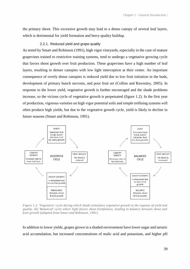
Chapter 1 - General Introduction |
39
the primary shoot. This excessive growth may lead to a dense canopy of several leaf layers,
which is detrimental for yield formation and berry quality buildup.
2.2.1. Reduced yield and grape quality
As noted by Smart and Robinson (1991), high vigor vineyards, especially in the case of mature
grapevines trained to restrictive training systems, tend to undergo a vegetative growing cycle
that favors shoot growth over fruit production. These grapevines have a high number of leaf
layers, resulting in denser canopies with low light interception at their center. An important
consequence of overly dense canopies is reduced yield due to low fruit initiation in the buds,
development of primary bunch necrosis, and poor fruit set (Collins and Rawnsley, 2005). In
response to the lower yield, vegetative growth is further encouraged and the shade problems
increase, so the vicious cycle of vegetative growth is perpetuated (figure 1.2). In the first year
of production, vigorous varieties on high vigor potential soils and simple trellising systems will
often produce high yields, but due to the vegetative growth cycle, yield is likely to decline in
future seasons (Smart and Robinson, 1991).
Figure 1.2. 'Vegetative' cycle during which shade stimulates vegetative growth at the expense of yield and
quality. (b) 'Balanced' cycle where light favors shoot fruitfulness, leading to balance between shoot and
fruit growth (adapted from Smart and Robinson, 1991).
In addition to lower yields, grapes grown in a shaded environment have lower sugar and tartaric
acid accumulation, but increased concentrations of malic acid and potassium, and higher pH
Chapter 1 - General Introduction |
40
values compared to non-shaded grapes (Smart, 1985). Substantial changes in secondary
metabolites involved in wine flavors and aromas are also noted, including polyphenols and
anthocyanins (Downey et al., 2006), skin flavonols (Diago et al., 2012), monoterpenes (Skinkis
et al., 2010), and norisoprenoids (Lee et al., 2007).
2.2.2. Increased cryptogamic disease pressure
A dense canopy usually contributes to the development of grape pathogens (Austin et al., 2011).
Uncinula necator and Plasmopara viticola are able to develop on leaf tissues, but also on green
stems, inflorescences, and fruit. Early season infections interfere with fruit set and cause
dramatic tield reductions if not controlled (Chellemi and Marois, 1992; Oliva et al., 1999).
Fungicide applications are usually necessary until the fruit reaches a certain degree of maturity,
although some varieties such as Muscat of Alexandria, Tokaz, Carignane, and Thompson
Seedless may be more resistant to infection (Chellemi and Marois, 1992; Gadoury et al., 2003).
Botrytis cinerea is another grapevine fungus whose growth is favored by dense canopies and
bunch compactness. This pathogen is especially damaging in cool climate regions with frequent
rain events late in the growing season, in many cases causing penalties in quality and yield. The
first symptoms of infection usually appear by the stage of veraison, and yield losses generally
occur because of stalk rot (leading to premature cluster fall) or losses of juice and berry
desiccation (Gubler et al., 1987). Botrytis cinerea converts glucose and fructose to gluconic
acid and glycerol and produces the Laccase enzyme that catalyzes the oxidation of phenolic
compounds, causing must browning (Zimdars et al., 2017). Botrytis cinerea also consumes high
quantities of yeast-assimilable nitrogen (YAN) and secretes polysaccharides such as β-glucans
that hinder wine fermentation and clarification due to their viscosity (Dimopoulou et al., 2017).
Several studies have shown that fruit grown in the shade is more prone to powdery/downy
mildew and bunch rot infection than fruits that are exposed to sunlight (Bavaresco et al., 2008;
Chellemi and Marois, 1992; Zahavi et al., 2001). In a trial on Vitis vinifera L. cv. Rielsing in
the Niagara region, Canada, (Percival et al., 1994) showed that machine-assisted leaf removal
at pea size stage on both sides of the fruiting zone of vigorous grapevines reduced the incidence
of bunch rot by as much as 20% and the percentage of clusters with slight symptoms by 17%.
In the case of powdery mildew, the phenomenon was explained in terms of plant-pathogen
interaction by the synergistic effects of UV-B radiation and the rise in temperature of exposed
grapevine tissues, both of which inhibit the development of fungi (Austin et al., 2009; Keller et
al., 2003). Other advantages of low canopy density are improved fungicide coverage of clusters

Chapter 1 - General Introduction |
41
and the possible increase in the volatility of sulfur due to the warming of exposed tissues, which
provides further suppression effects on the pathogens (Austin et al., 2011).
2.2.3. Higher management costs
Higher disease pressure, yield losses and grape quality reduction combined with vigorous and
long-lasting shoot growth all contribute to increase vineyard management costs. More elaborate
trellis systems like divided canopies are needed to support foliage weight and reduce canopy
shading. Summer pruning becomes necessary to allow machine circulation between rows and
make cultural operations like weed control, harvesting and foliage spraying more efficient.
However, this creates another problem since lateral shoot growth is favored by the trimming of
vigorous shoots, leading to more crowding in the remaining canopy (Poni et al., 2014). For this
reason, establishing a vineyard with the adequate parameters of planting density,
cultivar/rootstock combination, and management strategies is crucial for the long-term
productivity of the vineyard.
2.3. Achieving grapevine balance
Grapevine vigor is often regarded as a pejorative term, although neither low nor high shoot
vigor are necessarily undesirable as long as the grapevine produces a high yield of fruit at a
desirable quality, i.e. as long as it is balanced (Dry and Loveys, 1998). Balance from a
viticultural point of view can be expressed as the equilibrium between vegetative growth and
crop load. Although this concept has gained extensive attention in recent decades, it was first
imagined by Ravaz (1911) in the early 20th century, who devised a fruit to pruning weight ratio
as a practical method for winegrowers to evaluate grapevine balance. His concept has evolved
over time (Patridge, 1925; Shaulis, 1982) and is now also understood in terms of leaf area
needed to ripen a unit of crop weight (Kliewer and Dokoozlian, 2005; Petrie et al., 2000a, 2000b)
or leaf area per meter of canopy (Filippetti and Intrieri, 2001; Howell, 2001). Dry et al. (2004)
have reviewed grapevine balance indices that are commonly used in contemporary viticulture
(table 1.2). The general recommendation for the yield to pruning weight ratio (Y/P) is between
5 and 10, with values above this range leading to insufficient grape maturity. However, the
optimal Y/P ratio is highly dependent on planting conditions and genotypes. Low Y/P values
are associated with excessive vegetative growth, but studies have shown that values as low as
three may be optimal for cultivars with small bunches in cool climate (Kliewer and Dokoozlian,
2005). The leaf area to fruit yield ratio (LA/Y) and other ratios described in table 1.2 are
inversely related to Y/P, with higher values indicating excessive vigor.

Chapter 1 - General Introduction |
42
Table 1.2. Optimal ranges for various grapevine balance indices aggregated from various studies (adapted
from Dry et al., 2004).
Balance Index Abbreviation Optimal value
fruit weight per grapevine (kg) / pruning weight per
grapevine (kg)
Y / P 3 - 12
total leaf area per grapevine (m2) / fruit weight per
grapevine (kg)
LA / Y 0.6 - 1.5
pruning weight (kg) / unit of canopy length (m) P 0.3 - 1.0
total leaf area per grapevine (m2) / surface area per
grapevine (m2)
TLA / VSA < 2.5
total leaf area per grapevine (m2) / unit canopy length (m) - 2 - 5
mean cane weight (g) - 25 - 45
Several management practices can be employed to achieve grapevine balance. In cool climate,
the goal will often be to restrict grapevine vigor to avoid its negative consequences (Schultz,
1995), while it is more important in warm climate to ensure that the leaf area is sufficient to
optimally ripen the crop (Palliotti et al., 2014; Schultz, 1997).
2.3.1. Leaf and shoot removal
The vegetative growth cycle can be broken by reducing shade in the canopy directly or by
reducing grapevine vigor. Management practices such as shoot thinning and leaf removal are
cost-effective and flexible methods to achieve more open canopies (Bavaresco et al., 2008;
Nicolosi et al., 2012; Pellegrino et al., 2014). The amount of leaf area taken out can be relatively
precise and the location from where the leaves/shoots are removed (e.g. in the cluster zone or
above the cluster zone, inner leaves or outer leaves) can have more or less impact on vigor and
berry quality (Stoll et al., 2013). The main downside of these methods is that they can only
serve as temporary or ‘Band-Aid’ treatments to control excessive vigor since their effects only
last for a single growing season(Smart and Robinson, 1991). Defoliation around the cluster
zone can be performed manually or mechanically between fruit set and ripening in order to
expose clusters to sunlight and wind, and to improve spraying effectiveness (Bavaresco et al.,
2008; Percival et al., 1994). At veraison, leaf removal operations in very dense canopies resulted
in increased sugars, flavonoids, and aromas and lower acidity and botrytis and powdery mildew
infections (Austin et al., 2011; Percival et al., 1994; Poni et al., 2004; Stoll et al., 2013). In
addition to obtaining a more favorable canopy microclimate, this practice also modifies the
source/sink distribution and enhances the activation of light-induced enzymes such as the

Chapter 1 - General Introduction |
43
phenylanaline ammonia-lyase that participates in the formation of skin phenolic compounds
(Dokoozlian and Kliewer, 1995; Haselgrove et al., 2000).
Shoot thinning or ‘desuckering’ is usually performed in spring on water shoots (‘suckers’) that
compete with bearing shoots for grapevine resources and cause unfavorable shading (Smart and
Robinson, 1991). Shoot thinning can also be performed on bearing shoots, but only if crop load
is deemed excessive with regards to leaf area, in which case the practice is commonly called
‘summer pruning’. Depending on the cultivar, research reported reduced crop load and cluster
compactness as well as improvements in berry composition as a consequence of shoot thinning,
notably in the case of total soluble solids (TSS), total acidity (TA), and total polyphenols
(Morris et al., 2004; Reynolds et al., 2005; Sun et al., 2011; Tardaguila et al., 2008). However,
shoot thinning early in the season can have negative impacts on canopy microclimate in case
of high vigor, as remaining shoots will tend to grow longer and develop more laterals (Reynolds
et al., 2005).
Shoot trimming is another practice aiming to control vigor. It refers to cutting off the shoot
apical meristem in the summer to inhibit the growth of primary shoots and is usually performed
by machine. Shoot positioning must be done adequately beforehand, and varieties with an
upright behavior such as Cabernet Sauvignon are usually easier to manage (Poni et al., 2014).
Again, if performed in a high vigor situation, trimming will tend to trigger lateral growth near
the cutting position (Smart and Robinson, 1991).
2.3.2. Training system adaptation
A long-term alternative to leaf and shoot removal is to modify the training system and pruning
level to better counterbalance the effects of climate and vineyard potential.
It is well understood that pruning too severely in winter often leads to fewer but more vigorous
shoots (Winkler, 1974). Leaving a sufficient number of nodes in winter should lead to shoots
that are still growing after fruit set, but at a slow rate. Combined with a light trim in summer,
this method ensures that lateral growth is reduced (Palliotti et al., 2010). Increasing the number
of nodes is also the idea behind minimally pruned vineyards, where grapevines are not pruned
and shoots remain short and cease their growth around flowering (Poni et al., 2014; Smart and
Robinson, 1991). But increasing the number of nodes requires more space on the trellis to
prevent shading. This is possible with spur-pruned cordons but more difficult to apply in the
case of the Guyot training system.

Chapter 1 - General Introduction |
44
An alternative is the formation of divided canopies, which can ensure that a sufficient number
of nodes are retained without the risk of shoot crowding. By creating two or more canopies
from a single curtain, fruiting nodes can be better spread out in space, allowing for higher yield,
better light interception and resulting in higher fruitfulness and improved berry composition
(Smart, 1985). Notable examples of horizontally divided trellis systems include the Geneva
double curtain (GDC) and the lyre, and the vertically divided system in the Scott Henry
(Reynolds and Vanden Heuvel, 2009).
2.3.3. Root restriction
Intentional root volume restriction by using an artificial barrier that allows drainage has already
been used as a means to restrict the vigor of various fruit trees (Ismail and Davies, 1998; Yeh
and Chiang, 2001). Although experiments with container-grown grapevines demonstrated that
shoot growth was correlated to root volume regardless of the plant’s water and nutritional status
(Hatch et al., 2011; Yang et al., 2007), root restriction remains difficult to implement (Dry and
Loveys, 1998). Root pruning is easier to apply and was proven to be effective at reducing
grapevine shoot growth (Giese et al., 2015; McArtney and Ferree, 1999; Smart et al., 2006),
but is also not frequently used in commercial viticulture.
In regions where irrigation is beneficial for grapevine cultivation, deficit irrigation (DI),
regulated deficit irrigation (RDI) and partial rootzone drying (PRD) can be used to manage
vigor (Beis and Patakas, 2015). DI and RDI are based on controlling the water supply to induce
a light water stress during the growing season to reduce vegetative growth and improve berry
quality (Chaves et al., 2007). In DI, the same irrigation regime is applied thought the season
while in RDI water can be completely restricted during drought-insensitive phenological stages
like the end of the ripening period (Lopes et al., 2011). PRD aims to achieve the same benefits
by drying approximately half of the root system while the other half is still irrigated, and
switching between dry and wet side at regular time intervals (Stoll et al., 2000). The literature
suggests that DI, RDI, and PRD, depending on their timing and environmental conditions, are
useful techniques to increase grapevine water use efficiency while maintaining crop yield and
quality (Beis and Patakas, 2015; Chaves et al., 2010; Lopes et al., 2011).
2.3.4. Cover crop
Cover crops have been increasingly implemented in vineyards around the world in the last
decade. Whether purposely seeded or consisting of resident species that naturally cover the
vineyard floor, they bring about several benefits such as soil protection from erosion and

Chapter 1 - General Introduction |
45
crusting, improved soil fertility, structure, better water infiltration and water holding capacity.
Cover crops were also found to encourage soil biological diversity and the presence of
beneficial predators, weed suppression, and provide early firm footing for cultural operations
(Guerra and Steenwerth, 2011). Cover crops can also provide intentional competition for water
and soil nutrients to help regulate grapevine vigor (Ingels et al., 2005). The ability to choose
from a wide assortment of plant species comprising, among others, the Poaceae (cereals or
grasses) and Fabaceae (legumes) families, and the possibility to mow the cover crop anytime
during the growing season allows the adaptation of the timing and intensity of the competition
to best suit vineyard needs. In a trial by Hatch et al. (2011) on Cabernet Sauvignon in Virginia,
creeping red fescue (Festuca rubra) was associated to a permanent, mixed sward of tall fescue
(Festuca arundinacea) and orchard grass (Dactylis glomerata) as an under-trellis cover crop
(UTCC). The treatment was compared with a weed-free strip under the trellis obtained by
herbicide application. Results showed that UTCC was successful at suppressing vegetative
growth during the seasons of 2008 and 2009, as measured by rate and seasonal duration of shoot
growth, lateral shoot development, dormant pruning weights, and trunk circumference.
While cover crops can be used advantageously to control vigor in some situations, their effects
should be closely monitored to protect grapevines from uncontrolled competition that would
lead to undesirable reductions in capacity. In a study in Switzerland, the competition exerted
by a cover crop of tall fescue was too high for the grapevine, even with a deep soil and abundant
water resources (David et al., 2001). In order to prevent such a situation, cover crop species
should be selected while taking into account the timing and duration of their water use peak so
that it does not coincide with that of the grapevine (Celette et al., 2008).
3. Grapevine water relations
3.1. Cellular and physiological water transport mechanisms
Water constitutes a large fraction of a grapevine’s fresh weight and is involved in virtually all
the processes related to metabolism, including photosynthesis, thermal regulation, and ion
assimilation. At the cellular level, water transport occurs radially through apoplastic and cell-
to-cell pathways. The apoplastic pathway refers to water movement around protoplasts. The
cell-to-cell pathway combines two processes that are experimentally difficult to separate. The
first is the flow of water molecules through the cytoplasm and plasmodesmata between cells

Chapter 1 - General Introduction |
46
(symplastic pathway), while the second is the diffusion of water across the phospholipid bilayer
of cell membranes (transcellular pathway) (Steudle, 2000a; Vandeleur et al., 2009).
The cell-to-cell pathways are mostly regulated by aquaporins present in cell membranes. These
channel proteins, depending on their number and activity, allow the rapid diffusion of water
between cells (Gambetta et al., 2013). Several plasma membrane- and tonoplast-bound
aquaporins have been identified and functionally characterized in grapevine (Shelden et al.,
2009). In addition to water transport, specialized aquaporins can modify the concentration in
cells of specific solutes such as sugars, organic acids like malate, and inorganic ions like
potassium (K+) and chlorine (Cl-). Aquaporin ‘gates’ that are guarded by a negative charge are
impermeable to anions, while those that are guarded by a positive charge are impermeable to
cations (Maurel et al., 2008). As such, aquaporins are effective means of regulating the osmotic
potential (Ψπ) of cells.
Water is axially transported inside the grapevine through xylem vessels. The xylem is radially
connected to the apoplasts through a cell wall continuum, and is surrounded by parenchyma
cells that also contribute to water exchanges (Steudle, 2000a). Xylem water transport is largely
passive. In early spring, root water uptake is triggered by the release in the xylem sap of stored
reserves in the form of osmotically active ions and organic molecules. The differences in water
concentrations create an osmotic gradient throughout the grapevine and between the root
surface and the soil. This leads to a positive pressure that pushes water towards higher organs.
After leaf expansion, water uptake becomes mainly dependent on the hydraulic pull created by
leaf transpiration. By losing water to the atmosphere, the intrinsic leaf water pressure decreases,
which creates a pressure gradient that pulls water from lower parts of the grapevine (Keller,
2010).
3.2. Grapevine responses to water deficit
Grapevines experience water stress when the transpiration rate at the stomata exceeds the
absorption rate of water at the roots. In fact, transpiration consumes 95-98% of all the water
acquired by the grapevine, and it is the main driving force behind water movement during the
growing season (Keller, 2010). In order to limit water loss, grapevines are able to enact a series
of hydraulic resistances (figure 1.3). The main hydraulic resistance occurs at the leaf level with
stomatal closure (Steudle, 2000b). When Ψsoil declines, abscisic acid (ABA) is synthesized in
roots and shoots and is translocated through the xylem sap to the guard cells in the leaves to

Chapter 1 - General Introduction |
47
trigger stomatal closure (Chaves et al., 2010; Stoll et al., 2000). At the same time, ABA
promotes auxin-dependent root and root hair growth in order to increase soil volume
exploration and the size of the soil-root exchange surface (Lovisolo et al., 2016).
Figure 1.3. Schematic model of steady water flow through a plant, from soil to atmosphere. Water uptake
at the roots, long-distance transport in the xylem and stomatal resistances are represented as resistors of
relative resistance placed in series (Reproduced from Steudle 2000b).
The hydraulic pull at the leaf stomata leads to a hydraulic pressure difference between the roots
and xylem, and this pressure drives water through the roots using both apoplastic and cell-to-
cell pathways. In the absence of water stress, the cell-to-cell pathway is mostly used. This
pathway has a high hydraulic resistance to limit water losses to the soil, hence the ‘resistor’ in
the physics analogy of figure 1.3 (Steudle, 2000b).
The hydraulic resistance of the xylem is relatively small. However, xylem vessels are
susceptible to cavitation, a phenomenon that occurs during strong water deficits. When it
happens, the tension created by the transpiration rate and a dry soil separates the gas molecules
that are dissolved in the xylem sap. Cavitation reduces the grapevine’s capacity to transport
water, and if prolonged can cause irreversible damage to xylem vessels (Brodersen et al., 2010).

Chapter 1 - General Introduction |
48
Isohydric genotypes like Grenache or Tempranillo can better modulate their stomatal
conductance and prevent cavitation more easily than anisohydric genotypes like Syrah,
Chardonnay, or Riesling (Lovisolo et al., 2010; Schultz, 2003; Vandeleur et al., 2009).
It is worth noting that isohydricity has been defined in many ways over time, which can shift
the classification of cultivars on its scale. For example, Tardieu and Simonneau (1998)
described it as the ability (or its lack) to maintain a constant midday water potential (ΨMD) when
Ψsoil declines, while Martínez-Vilalta et al. (2014) used the slope σ of ΨMD and predawn water
potential (ΨPD) in their definition (σ < 1 isohydric). Furthermore, contradicting research has
recently shown that cultivars may behave differently depending on climatic conditions (Chaves
et al., 2010; Hochberg et al., 2018), somewhat blurring the iso/anishohydric distinction.
4. Berry development and composition
4.1. Berry structure
The grape berry begins its development after fecundation of the ovary (fruit set). The ovary
wall develops into the fruit wall or pericarp, which is in turn divided into the external exocarp
(the skin), the mesocarp in the middle (the flesh), and the inner endocarp (the seeds and the
tissue that surrounds them) (figure 1.4). The exocarp is made of two anatomically distinct
regions, the epidermis and the hypodermis. The former is made of a single uniform layer of
cells, while the latter is thicker and is the main storage organ for several secondary metabolites
such as anthocyanins (responsible for the red pigmentation of certain cultivars), flavonols, and
various aroma precursors (Coombe, 1987; Downey et al., 2006; Kennedy, 2002; Ollat et al.,
2002).
The mesocarp represents the majority of the weight of ripe berries. Its parenchymatic cells are
responsible for the storage of sugars, organic acids, and nutrients in their large vacuole, which
can make up as much as 99% of the total cell volume at maturity (Jackson, 2008; Ollat et al.,
2002).
The endocarp in the innermost tissue of the pericarp and represents the seeds and their
surrounding locules. The seeds are made of an epiderm and a pair of integuments that
encapsulate the embryo and the endosperm. The seeds only accounts for a small portion of the
berry weight (Cadot et al., 2006).

Chapter 1 - General Introduction |
49
Figure 1.4. Schematic representation of the grape berry at maturity (reproduced from Coombe, 1987).
4.2. Berry development
Berry growth follows a double-sigmoid curve (figure 1.5). In stage I, which typically lasts
between six weeks and two months, berry cells divide rapidly and increase in size while the
endosperms forms (Coombe and McCarthy, 2000; Kennedy, 2002; Ollat et al., 2002). These
changes are accompanied by an accumulation of tartaric and malic acid in the mesocarp.
Tartaric and malic acids are predominant at all stages of the berry development and have the
largest influence on juice acidity (Sweetman et al., 2014). Phenolic compounds such as
flavonoids and hydroxycinnamic acids are also accumulated (Downey et al., 2006). Chlorophyll
is the major berry pigment during stage I. In fact, throughout this initial phase berries are able
to produce the carbon necessary for their growth via photosynthesis (Kliewer, 1965).

Chapter 1 - General Introduction |
50
Figure 1.5. Diagram showing the double sigmoid growth curve of berry development, including the timing
of accumulation of metabolites and indications of xylem and phloem inflow rates (reproduced from
Kennedy, 2002).
The first growth phase is followed by a latent phase (stage II) during which the growth rate of
the berry is diminished while the embryos develop and the seed coats harden (Ollat et al., 2002).
This stage can vary between one to six weeks depending on the cultivar and largely decides if
a cultivar has an early or late maturing character (Jackson, 2008). The second stage ends with
veraison, the inflection point at which the berry begins to lose its green color. The change of
color represents a fundamental shift in berry metabolism that ultimately leads to maturity (stage
III); the berries lose their ability to enact photosynthesis. Instead, water and sucrose produced
by surrounding leaves are imported through the phloem, which significantly increases the
volume of mesocarp vacuoles (Kliewer, 1965). Sucrose is hydrolyzed to glucose and fructose
inside the apoplast or the vacuole by the invertase enzyme (Conde et al., 2007). Malic acid,
having reached its peak concentration just before veraison, is gradually degraded in stage III to

Chapter 1 - General Introduction |
51
be used as a potential carbon source for respiration and/or glucogenesis (Sweetman et al., 2014).
The degradation of malic acid and the dilution of tartaric acid contribute to the increase in juice
pH during ripening (Kliewer, 1965).
In addition to sugar accumulation and the decrease in organic acid concentration, the third stage
is also the stage at which phenolic compounds and aroma compounds are synthesized in the
exocarp (Ollat et al., 2002). Phenolic compounds are derived through the phenylpropanoid
pathway from the amino acid phenylalanine. The compounds produced from phenylalanine are
classified as stilbens and flavonoids, the latter of which includes anthocyanins, flavonols,
flavan-3-ols, and proanthocyanidins (Flamini et al., 2013).
Flavonols are a family of compounds that play a protective role against UV radiation in the
plant kingdom by acting as radical scavengers (Downey et al., 2006; Haselgrove et al., 2000).
They are yellow pigments that contribute directly to the color of white wine and indirectly to
the color of red wine by copigmentation with anthocyanins. Flavanols mostly found in grape
berries and wine are the glycosylated forms of quercetin, kaempferol, isorhamnetin, myriecetin,
laricitrin, and syringetin with the glycones 3-O-glycosyl, 3-O-galactosyl, and 3-O-gycuronyl
(Castillo-Muñoz et al., 2010). Quercetin derivatives are generally predominant in wine (Mattivi
et al., 2006).
5. The Riesling cultivar
Riesling is believed to be native of the Rheingau valley of Germany. The oldest written
reference to the cultivar, or at least one of its close progenitors, was the word ‘Rießlingen’ on
cellar accounting documents dating from March 13, 1435 that were addressed to the Earl of
Katzenelnbogen in Rüsselsheim am Main (Staab, 1991, 1986). Genetic analyses have
established Riesling as having a parent-offspring relationship with Gouais Blanc, who is
genetically related to at least 80 other grape varieties including Chardonnay and Gamay
(Boursiquot et al., 2004). Another hypothesis suggest that Riesling may be a progeny of
Traminer brought by the Romans to the Rhine region and a frost resistant, small-berry,
autochthonous cultivar that was cultivated by German tribes. The resulting cultivar is thought
to have been further interbred with Heunisch to increase its consistency, vitality and acid
potential to become the Riesling that is cultivated today (Lott et al., 2010).
Riesling has erect shoots with fairly short internodes. Its mature trapeze-shaped leaves are dark
green in color with a closed petiolar sinus. Its clusters are relatively small, compact and

Chapter 1 - General Introduction |
52
cylindrical, often with one or two wings. The berries are small with a thick light-yellow skin
(Schneider et al., 2012). Riesling is a late-ripening variety compared to other German cultivars
like Müller-Thurgau. Its budbreak is also quite late, which makes it less prone to spring frost.
In cold climate regions, Riesling needs a sufficient quantity of warmth during the growing
season order to fully ripen, but excessive hot weather is generally detrimental to fruit quality
(Ambrosi, 2011). Riesling is not particularly vulnerable to pests and diseases such as downy
and powdery mildew, but bursting berries are frequent in years with high humidity, which may
lead to higher susceptibility to Botrytis cinerea infections (Lott et al., 2010).
The global Riesling vineyard area is estimated around 64000 ha (OIV, 2018b). Germany
accounts for 36.9% of this value, followed by Romania, the USA, France, and Australia (table
1.3). At the country scale, 23.3% of Germany’s vineyard area is allocated to the variety, making
it the most important cultivar in the country (Deutsches Weininstitut, 2017; OIV, 2017).
Table 1.3. Top five countries by Riesling vineyard area in 2015 (data sourced from OIV, 2018b, 2017).
Country Riesling vineyard area
(ha)
% World Riesling area % Country vineyard
area
Germany 23596 36.9 23.3
Romania 6121 9.6 3.1
USA 4605 7.2 1.0
France 4025 6.3 0.5
Australia 3157 4.9 2.0
5.1. Varietal aromas of Riesling
The aroma of Riesling wines reflect the soil, climate, and management practices that produced
them (Douglas et al., 2001; Fischer et al., 1999). Because of this close relationship with ‘terroir’,
it is difficult to define a very specific character for this grape variety, but some general
characteristics can be extracted from the literature. For example, Riesling wines that are
produced in cool climates tend to have low alcohol and a high degree of acidity, giving them a
distinct brightness and clarity in the mouth (Robinson et al., 2013). On the other hand, Rieslings
such as those coming from the Pfalz region of Germany are more intense and full-bodied, with
aromas ranging from floral to honey-like. Other aromas that are frequently described in Riesling
wines include the citrus, stone and exotic fruit families, as well as vegetal aromas like freshly
cut grass and hay (Schüttler et al., 2015). When aged, Riesling wines have a uniquely

Chapter 1 - General Introduction |
53
characteristic profile as they develop aromas of dried fruits and the so-called ‘kerosene’ aroma,
the hallmark of the cultivar (Lott et al., 2010).
The varietal aromas of Riesling wine are derived from multiple classes of volatile compounds
including monoterpenes, norisoprenoids, and volatile thiols (Schüttler et al., 2015).
5.1.1. Monoterpenes
Monoterpenes are organic C10 compounds that belong to a large group of chemicals known as
terpenoids, which also includes norisoprenoids. The first step of monoterpene biosynthesis
occurs with the formation of isopentenyl pyrophosphate (IPP) through either the cytosolic
melavonate pathway or the plastidial methylerythriol pathway (Duchêne et al., 2009). The
second step involves the synthesis of geranyl phosphate (GPP) by condensation of IPP and its
isomer dimethyl allyl diphosphate (DMAPP). Monoterpenes are produced from GPP through
the action of terpene synthase (Robinson et al., 2014). The Vitis vinifera (VvTS) terpene
synthase gene family is reportedly involved in the production more than 21 monoterpenes
(Martin et al., 2010). Other genes like the ones coding for deoxy-D-xylulose synthase (VvDXS)
are also known to be associated with the early steps of terpene production (Emanuelli et al.,
2010).
Plants rely on monoterpenes for a variety of functions, from deterring animals to protecting
against fungal and bacterial infections (Gershenzon and Dudareva, 2007). Indeed, recent studies
have shown that volatile monoterpenes and sesquiterpenes are emitted by in vitro-grown plants
after inoculation with P. viticola strains, and that the nature and quantity of emitted quanpounds
depended on the grapevine genotype (Algarra Alarcon et al., 2015). The most common
monoterpenes in grapes and wine are the monoterpene alcohols linalool, α-terpineol, nerol,
geraniol, citronellol and hotrienol. Some of those compounds also form isomeric oxides like
linalool oxide (cis-, trans- in pyranoide and furanoide forms) and nerol oxide (Bakker and
Clarke, 2011). Monoterpenes are mainly found in berries as odorless glycoside conjugates. The
odor-active aglycones can be released by enzymatic or acidic hydrolysis during wine
fermentation and storage (Black et al., 2015).From a winemaking perspective, monoterpenes
play a major role in the aroma of Muscat varieties and non-Muscat aromatic varieties like
Gewürztraminer and Riesling (Mateo and Jiménez, 2000), with high levels of linalool and α-
terpineol being positively correlated with flowery aromas (Günata et al., 1985).

Chapter 1 - General Introduction |
54
5.1.2. Norisoprenoids
Norisoprenoids (C13) are degradation products of carotenoids, which participate in the light
harvesting activity of chloroplasts and protect the cell from photo-oxidative damage
(Lashbrooke et al., 2013). Norisoprenoids consist of a megastigmane skeleton and can have
various olfactory properties depending on the position of an oxygen group. Damascenones are
norisoprenoids with the oxygen group bound to carbon 7, while ionones have the oxygen group
bound to carbon 9 (Winterhalter et al., 1990).
Two norisoprenoids of particular importance for wine are β-damascenone and β-ionone, which
contribute to fruity and flowery notes (Mendes-Pinto, 2009). The typical ‘kerosene’ aroma of
Riesling wine is due to the norisoprenoid 1,1,6-trimethyl-1,2-dihydronaphtalene (TDN). This
compound, which is barely present in free form in berries, is obtained by the hydrolysis and
rearrangement of glycosylated precursors during winemaking and aging (Sacks et al., 2012).
5.1.3. Volatile Thiols
Thiols are sulfur-containing molecules that are widely represented in food products beverages
and are often characterized by low odor thresholds (Vermeulen et al., 2005). Several odorous
thiols were identified in Sauvignon Blanc wines and later in wines from Semillon, Riesling, and
Pinot Gris, and Colombard with varying concentrations (Tominaga et al., 2000). Among these
thiols, 4-methyl-4-sulfanylpentan-2-one (4MSP) and 3-sulfanylhexan-1-ol (3SH) contribute
respectively to Sauvignon Blanc box-tree and passion fruit aromas (Helwi et al., 2016). They
are obtained by cleavage of odorless precursors, namely S-conjugates to glutathione and
cysteine, during fermentation (Robinson et al., 2014; Roland et al., 2011).

Chapter 1 - General Introduction |
55
6. Objectives of the thesis
The research objectives of the present work were to investigate the impact of grapevine age on
its leaf physiology, water tolerance, vegetative growth, vine balance, and berry and wine quality.
For this purpose, a dedicated vineyard planted in Geisenheim, Germany for this very purpose,
with Vitis vinifera L. cv. Riesling grapevines of the same plant material but planted in 1971,
1995 and 2012 was studied between years 2014 and 2017.
More specifically, the four objectives of this work are were:
1. to follow the productivity and vegetative growth of the three grapevine age groups over
time, and examine their response to an induced water stress;
2. to analyze and compare the canopy and cluster architectures among the three grapevine
groups and assess the effects of these parameters on berry composition and enological
potential;
3. to chemically analyze and sensorially evaluate wines produced from the three grapevine
age groups, both from recent (2014 to 2017, all three groups) and older vintages
(predating 2014, only for grapevines planted in 1971 and 1995);
4. to develop and test a non-destructive, structure-from-motion with multi-view stereo-
photogrammetry-based method that could be used as a tool directly at the vineyard to
complement traditional dendrology measurements.

Chapter 2 - Impact of grapevine age on water status and productivity |
56
Chapter 2. Impact of grapevine age
on water status and productivity
This chapter has been published in a modified version as:
Bou Nader, Khalil, Manfred Stoll, Doris Rauhut, Claus-Dieter Patz, Rainer Jung, Otmar
Loehnertz, Hans Reiner Schultz, et al. “Impact of Grapevine Age on Water Status and
Productivity of Vitis vinifera L. Cv. Riesling.” European Journal of Agronomy 104 (March 1,
2019): 1–12. https://doi.org/10.1016/j.eja.2018.12.009.
Author contributions: the author designed and conducted the research experiments, analyzed the
data, drafted and constructed the manuscript. ELISA analysis was performed by Dr. Elvira
Bleser and Johannes Kiesgen (Department of Grapevine Breeding, HGU) and carbon
discrimination analysis was performed by Olivier Mathieu (Biogeosciences, CNRS/University
of Burgundy).
Chapter 2 - Impact of grapevine age on water status and productivity |
57
1. Abstract
Grapevines are perennial plants that can display remarkable longevity. It is often thought that
some of their characteristics evolve in a positive way as they grow older, such as having a
higher tolerance to water deficit and an improved balance between vegetative and reproductive
growth. However, only a few studies have been conducted so far on the possible effects of age
on vine productivity and water status.
An experimental vineyard was designed in the German Rheingau region to compare vines of
identical planting material planted at three different times. The vineyard was established in
1971 with Vitis vinifera (L.) cv. Riesling vines (clone Gm 239-17) grafted on 5C Teleki and
trained in double Guyot and cordon in alternating rows. In 1995 and 2012, rows of both training
systems were uprooted and replanted with the same scion/rootstock combination. The aim of
this study was to evaluate the impact of vine age on several physiological and reproductive
parameters. Vines planted in 2012 were generally more sensitive to water deficit than vines
planted in 1995 and 1971, although this depended on the amount of precipitations during the
growing season. A supporting trial was carried out to create more intense drought conditions
by deploying a plastic mulch around selected vines during rain events. Young vines were most
affected by the treatment, suggesting that their lower tolerance to water deficit might be due to
a shallower root system. Vines planted in 1995 and 1971 displayed similar response to water
deficit. Canopy architecture, cluster parameters and vine balance components including pruning
weight and yield were different for the youngest vines until the fifth year after planting due to
their lower cropping capacity. Even though the observed yield and pruning weight per meter
were lower for grapevines planted in 1971 than those planted in 1995, these variables were
similar across the two age groups when missing vines were taken into account. Wood diseases
were identified as the main factor behind the decline of old vines. The study suggests that the
management of wood diseases is a key component in improving vineyard longevity, and that
the conservation of grape yield and technological maturity parameters for vineyards in similar
environmental conditions is indeed possible over the long term.
Keywords: old vine, water deficit, balance, vigor, capacity, trunk disease.
2. Introduction
Grapevines can thrive over several centuries while still producing wine (Grigg et al., 2017;
Robinson et al., 2013; Vršič et al., 2015). Despite their longevity, it is not uncommon today to

Chapter 2 - Impact of grapevine age on water status and productivity |
58
see vineyards uprooted only two to three decades after planting. Sometimes the goal may simply
be to replant them with cultivars that better fit wine consumption trends, but the decision can
also be due to declining grape production (Bernizzoni et al., 2009; Duthie et al., 1991). Indeed,
a number of external factors may, on their own or in combination, lead to significant losses in
their economic viability (Kaplan et al., 2016). These factors include wood diseases such as esca,
eutypa dieback, and botrysphaeria dieback (Bertsch et al., 2013) and viral diseases that can
prove damaging once their vectors are well established (Credi and Babini, 1997; Walker et al.,
2004). In some cases, poor management practices may result in dense canopies and compact
soils, reducing the value of the crop while escalating production costs (Morlat and Jacquet,
2003; Smart and Robinson, 1991).
While it may be difficult to manage vineyards over long periods of time, the benefits of doing
so from a viticultural and enological perspective remain unclear. Nevertheless, a growing body
of research on grapevine age has developed over the last 15 years, with a focus on berry
metabolites and wine sensory attributes (Du et al., 2012; Heymann and Noble, 1987; Reynolds
et al., 2008; Zufferey and Maigre, 2008). Other studies have investigated the influence of vine
age on its vegetative and reproductive performance. For instance, Zufferey and Maigre (2007)
recorded higher net photosynthesis, predawn water potential, and pruning weight for older vines,
while Grigg et al. (2017) noted the tendency of old vines to form higher fruit yields, with the
possible explanation of increased wood reserves. Some of these results contrasted with other
research that described older vines as equally or less vigorous than young vines (Considine,
2004; Ezzili, 1992). The apparent disparities in the literature may arise from the difficulty in
finding adequate plant material and designing field experiments about vine age with
comparable conditions. As a consequence, the vine ages that are referred to as ‘young’ and ‘old’
vary widely among studies. In addition, the plant material of old vineyards can be difficult to
acquire decades later, unless the vines are own-rooted. For grafted vines, the nature of the scion
and rootstock combination can also influence vine longevity (Lider et al., 1978), which adds
another layer of complexity to experimental conditions. Finally, the effects related to vine age
can be difficult to separate from seasonal and site variability (Grigg et al., 2017; Reynolds et
al., 2008).
A major source of climatic variation is water availability, reflected by the timing and intensity
of precipitation events. High water deficits over the growing period can inhibit shoot growth
and photosynthesis (Keller et al., 2016; Schultz and Matthews, 1988) and negatively affect yield

Chapter 2 - Impact of grapevine age on water status and productivity |
59
and berry composition (Marciniak et al., 2013; Romero et al., 2015). Previous research
suggested that young vines were more sensitive to drought, possibly because of a less developed
root system (Zufferey and Maigre, 2007), but experiments comparing groups of older vines
have not yet been undertaken. In order to systematically investigate the influence of vine age
on water status, this paper reports on a unique Riesling vineyard with alternating rows of vines
of identical planting material, but with three planting years ranging from 1971 to 2012. It also
includes two training systems, the double (bilateral) Guyot and the single spur-pruned cordon.
The main goal of the present work, which focused on the Guyot vines, was to compare the three
vine age groups with respect to their tolerance to water deficit and vine productivity as
described by canopy architecture, cluster parameters, pruning weight, and yield from 2014 to
2017. The second part of this work was designed as a supporting experiment on the cordon
trained vines to investigate drought tolerance, which was achieved by deploying a plastic mulch
during rain events around a subset of vines in 2016 and 2017 and monitoring the vines’ behavior
with respect to the absence of precipitations.
3. Materials and methods
3.1. Weather data
The trial was conducted in Geisenheim, Germany (49° 98’ N, 07° 94’ E) in an experimental
vineyard managed by the Department of General and Organic Viticulture of Hochschule
Geisenheim University (HGU). Daily temperature, precipitation, and wind speed data were
recorded by a local weather station belonging to HGU and located around 500 m east of the
vineyard. The temperature information was used to compute the growing degree-day (GDD)
accumulation from April 1st to October 31st by subtracting a base temperature of 10 °C from
the daily average temperature (Jones, 2005; Winkler, 1974).
3.2. Experimental design and plant material
The experimental vineyard was established in 1971 with Vitis vinifera (L.) cv. Riesling (clone
Gm 239-17) grafted on 5C Teleki rootstock (Vitis berlandieri × Vitis riparia) in well-drained,
fertile clay loam soil (270 g kg-1 clay, 410 g kg-1 silt, 260 g kg-1 sand, with a pH of 6.9, and
wilting point and field capacity of 0.15 and 0.30 m3 water m-3 soil, respectively). The vines
were planted along 68 rows in a North-South orientation coinciding with a downward slope of
eight degrees, an inter-row distance of 2.00 m, and vine spacing of 1.40 m. Two pruning
systems were managed on the same plot: the double (bilateral) Guyot with downward arched
Chapter 2 - Impact of grapevine age on water status and productivity |
60
canes, and the single cordon with two-node spurs. In 1995 and 2012, several rows of vines were
uprooted and replanted with the same combination of clone and rootstock. The end result was
a vineyard with alternating rows of vines of different ages and pruning systems. Each combined
treatment (planting year × pruning system) was available in four field replicates.
The trial on double Guyot vines started in 2014, which was the first productive year of vines
planted in 2012. At that time, some vines were already missing in the rows planted in 1971 and
1995. A fully randomized block experimental design was therefore not possible to implement.
Instead, a selection process was carried out at the beginning of the 2014 growing season in
order to choose six double Guyot vines per age group and field replicate for seasonal
measurements (n = 24). The number of nodes retained was adjusted to 10 per meter (equivalent
to 14 nodes per vine) during winter pruning. The trunk diameter measured 10 cm above the
grafting point (Santesteban et al., 2010) and the bud fruitfulness of individual vines were
compared to the median and mean values of their respective rows, and the three vines closest
to these values were selected. Trunk size is commonly used to estimate the vigor of perennial
plants. It was used at the beginning of the 2014 growing season to select vines that were most
representative of their respective populations, especially for vines planted in 1971 which had
the largest heterogeneity in size. Bud fruitfulness, being directly related to inflorescence
number and fruit production (Sánchez and Dokoozlian, 2005) was also considered as a selection
parameter. However, since it is much more sensitive to external factors such as late frost
damage and is affected by the environmental conditions of the previous season (May and
Antcliff, 1963) this variable only played a minor role in vine selection.
Vines close to the edges of the vineyard and those adjacent to the empty spaces left by missing
vines were used as buffer and were not included in measurements. The health status of selected
vines was visually appraised for trunk diseases and viral infections. In 2017, the selected vines
were also inspected by Enzyme-Linked Immunosorbent Assay (ELISA) tests (Clark and Adams,
1977) for potential infections of Arabis Mosaic Virus (ArMV), Grapevine Fleck Virus (GFkV),
Grapevine Leafroll-Associated Virus 1 and 3 (GLRaV-1, GLRaV-3), and Grapevine Flanleaf
Virus (GFlV). The tests were made on dormant shoot cuttings that were collected prior to winter
pruning.
Due to the general vigor of the site, a cover crop of grass and clover was sown in alternating
rows when the vineyard was established with a weed-free strip of about 10 cm under the rows.

Chapter 2 - Impact of grapevine age on water status and productivity |
61
When the second group of vines was planted in 1995, their rows were tilled in the first two
years to prevent excessive competition with cover crop during the early developmental stages
of the vines (Williams et al., 1990). The same treatment was applied from 2012 to 2014 in the
rows of the youngest vines. Afterwards, these rows were sown with the same cover crop
combination that already existed in 1995 and 1971 rows. In order to assess the impact of cover
crop over time, the soil nitrate content at depths of 0 to 30 cm and 30 to 60 cm was used as
indicator for nitrogen mineralization (Stenberg et al., 1999; Wehrmann and Scharpf, 1986). It
was measured from 2014 to 2017 at flowering, veraison, and harvest. Fifteen soil samples per
field replicate (n = 4) were combined with a soil homogenizer (Schäfer, Euskirchen, Germany)
and analyzed according to Schaller (1988) by flow injection at 450 nm with a Tecator FIAstar
Analyzer® (FOSS, Hillerød, Denmark). The fresh weight was taken at the time of measurement,
after which soil samples were dried in a laboratory stove at 80 °C until mass stabilization. The
difference between wet and dry weight was recorded for each sample to calculate soil water
content. The leaf chlorophyll index under green excitation (SFR_G) of three healthy, mature
leaves per selected vine was also assessed every two weeks from berry set to harvest with a
Multiplex Research® portable sensor array (Force-A, Orsay, France) set to leaf measurement
with an aperture of 4 cm (n = 24). The data was collected between 0900 and 1200 hr on the
eastern side of the canopy on fully illuminated leaves. The vine measuring order was
randomized to account for diurnal variability. Phenology was followed on 50 random vine
organs per double Guyot and cordon row on a weekly basis until veraison according to the
modified E-L system developed by Coombe (1995) that simplifies previous systems (Baggiolini,
1952; Lorenz et al., 1995).
3.3. Gas exchange measurements
The leaf CO2 assimilation rate (AN), stomatal conductance (gs), and transpiration rate (E) of
selected vines were followed during the 2016 and 2017 seasons using a LI-6400XT®
photosynthesis system (LI-COR, Nebraska, USA). The measurements were made in a 6 cm2
chamber at ambient CO2 concentration and photosynthetically active radiation (PAR). Block
temperature was controlled at 30 °C, which resulted in leaf temperatures between 29 and 30 °C.
3.4. Vine capacity and balance
Leaf and cluster distribution in the cluster zone were determined at veraison by point quadrat
analysis (Meyers and Vanden Heuvel, 2008; Smart and Robinson, 1991). A measuring tape was
extended along the cluster zone at a fixed height and a thin, sharpened metal rod was passed

Chapter 2 - Impact of grapevine age on water status and productivity |
62
horizontally through the canopy from end to end. A total of 50 insertions were made per row,
with a distance of 20 cm between insertions. Contacts with leaves, clusters, and canopy gaps
were recorded and used to calculate percent gaps (PG), leaf layer number (LLN), percent
interior leaves (PIL) and percentage interior clusters (PIC). Point quadrat analysis could not be
performed in 2017 due to a severe infection of downy mildew around flowering and berry set,
which forced a partial defoliation of the cluster zone for all grapevines. Cluster parameters were
assessed yearly around two weeks before harvest in order to ensure the availability of healthy
clusters. Four clusters per row were randomly selected. After weighing and destemming, the
number of berries per cluster and their average weight were recorded.
Harvest date was chosen yearly according to the technological maturity (with general targets of
23 °Brix, titratable acidity of 9 g tartaric acid eq. L-1 and pH 2.9 for dry Riesling wine) and the
disease status of the grapes. The double Guyot rows were harvested by hand while sorting out
healthy and rotten berries. Both yield fractions were weighed separately, and only healthy
berries were used in winemaking. Pruning weight per vine and average cane weight were
recorded during winter pruning. The adjusted values of pruning weight and yield, both of which
account for the number of missing vines per row, were also calculated.
3.5. Berry technological maturity and δ13C
Berry samples were collected at harvest from individual rows for maturity analysis and dry
mass carbon isotope discrimination (δ13C). Maturity analysis was made on fresh berries. Juice
total soluble solids (TSS) was determined for each sample with a refractometer (Kübler,
Karlsruhe, Germany). Titratable acidity (TA) and pH were assessed with a 719 S Titrino
terminal titration unit (Metrohm AG, Herisau, Switzerland). The α-amino nitrogen content was
determined by o-phthaldialdehyde/N-Acetyl-L-Cysteine spectrophotometric assay (NOPA),
according to Dukes and Butzke (1998). For δ13C the juice obtained at harvest was frozen until
analysis, which followed the method described by Gaudillère et al. (2002). The samples were
prepared at the joint research unit of Vine Ecophysiology and Functional Genomics (EGFV) of
the Institute of Vine and Wine Sciences (ISVV) in Bordeaux, France, and analyzed with a
Vario® elemental analyzer (Elementar, Hanau, Germany) coupled with a continuous-flow
isotope mass spectrometer (Isoprime, Manchester, UK). This latter part was subcontracted to
the joint research unit Biogeosciences (National Center for Scientific Research CNRS/
University of Burgundy) in Dijon, France. The instrument was calibrated with isotopic

Chapter 2 - Impact of grapevine age on water status and productivity |
63
reference materials of L-glutamic acid (USGS40; δ13C = -26.389 ± 0.042 ‰) and caffeine
(IAEA-600; δ13C = -27.771 ± 0.043 ‰).
3.6. Experiment on water deficit
In 2016 and 2017, a separate field experiment on water deficit was carried out on the cordon
trained rows. Eight consecutive vines were selected within these rows in 2016 with criteria
similar to the double Guyot vine selection and the same number of retained nodes. White
foldable plastic sheets were installed in the first week of May around four of those vines, with
an approximate covering area of 20 m2 (“stress”, appendix 2.1). During the growing season the
plastic sheets were extended to cover the soil during rain events and were otherwise folded to
avoid condensation. The other four vines remained uncovered for the duration of the experiment
(“control”, appendix 2.1). The two central vines from each treatment were used for
measurements (n = 8). Soil samples were manually collected at flowering, pea-size berries and
two weeks after veraison for the estimation of water content for the stressed and control
treatments. A Pürkauer auger was used between the center vines on the eastern and western
sides of the rows, and samples were collected from 0 to 30 cm and from 30 to 60 cm. The
chlorophyll index was monitored on the central vines of each treatment on the same dates as
the double Guyot vines as described above.
Leaf stomatal conductance was assessed on cordon vines using an AP4® porometer (Delta-T,
Cambridge, UK) that was calibrated in the vineyard prior to measuring. Predawn water potential
(ΨPD) was measured on cordon vines using a Scholander pressure chamber connected to a
nitrogen gas cylinder (Soil-Moisture Corporation, Santa Barbara, CA, USA; following the
principle of Scholander et al., 1965) on several dates over the growing season. Measurements
were made on dry, mature leaves of the two center vines of the control and stressed treatments.
The negative value of the pressure required to force sap from the petiole (in MPa) was recorded
as the water potential. The berry δ13C at maturity was assessed for the three age groups of vines
and the two water treatments following the protocol described earlier.
3.7. Statistical analysis
Linear mixed-effect models (LMM) were used to evaluate the effect of vine age on the
parameters of interest. Vine age and year were converted to categorical variables and used as
fixed effects in all models. Water status was added as a fixed effect with two levels (control and
stressed) for data related to the water deficit trial on cordon vines. For measurements that were

Chapter 2 - Impact of grapevine age on water status and productivity |
64
repeated along the growing season, random effects were structured to account for space and
time variability (Schielzeth and Forstmeier, 2009). Single vines were included as a nested
random effect inside blocks. The dates of measurement or phenological stages were grouped
and converted to a factor that was used as a crossed random effect. A similar approach was used
in the case of yearly measurements such as fruit yield and pruning weight, with both vine age
and year as fixed effects and block as a random effect. Model parameters were estimated by
restricted maximum likelihood (REML) in R (R Core Team, 2018) with the packages lme4
(Bates et al., 2015) and pkbrtest (Halekoh and Højsgaard, 2014). The importance of fixed
effects was assessed by Kenward-Roger approximations at a significance level of P = 0.05
(Schaalje et al., 2002). Variation around means was reported as standard deviation (sd).
Principal Component Analysis (PCA) was used to examine the relationship between point
quadrat analysis, cluster parameters and grapevine balance components. PCA was performed
with the packages FactoMineR (version 1.41; Lê et al., 2008) and factoextra (version 1.0.5;
Kassambara and Mundt, 2017).
4. Results
4.1. Weather data
The year 2014 had the highest growing degree-day (GDD) accumulation from April 1st to
October 31st (table 2.1), with high temperatures around flowering. Although mean daily
temperatures in July were above average during this growing season, they were the lowest of
all years in August, with elevated precipitation levels for these two months.
Table 2.1. Growing degree-day (GDD) and precipitation data for Geisenheim Fuchsberg, Germany, from
April 1st to October 31st for the growing seasons 2014-2017. The yearly average represents the period of
1981-2010.
Growing season GDD Precipitations (mm)
2014 1366 447
2015 1359 239
2016 1358 358
2017 1345 363
yearly average (1981-2010) 1119 336
The year 2017 had the second highest cumulative precipitations during the growing season, but
it was also the coolest on average, with low temperatures between flowering and veraison. The
growing seasons of 2015 and 2016 were the warmest on average, with mean daily temperatures

Chapter 2 - Impact of grapevine age on water status and productivity |
65
close to 30 °C and maximal temperatures above 35 °C for several days in July and August
(appendix 2.2). Precipitation levels in the growing season were lowest in 2015 with only 239
mm of rain. Although the year 2016 was fairly rainy compared to the long-term average, most
precipitation events occurred at the beginning of the growing season, with warm and dry
conditions from fruit set to harvest. Budburst occurred at its earliest on April 7th in 2014, while
the latest budburst date was recorded in 2016 on April 22nd. Other phenological events, notably
flowering and veraison, took place at similar times in all growing seasons. Among the three age
groups and two training systems, vines planted in 2012 were consistently two to three days
more advanced for budburst, flowering, and veraison compared to vines planted in 1971 and
1995.
4.2. Vine selection and soil management
The trunk diameter of double Guyot vines planted in 2012 showed low variability in 2014
(figure 2.1). Trunk variability was higher for other age groups, with values ranging from 34.4
to 82.7 mm for vines planted in 1971. Although the nodes retained at pruning were limited to
14 per vine, the mean number of fruitful buds per vine in spring 2014 was 13.4, 11.5, and 7.0
for vines planted in 1971, 1995, and 2012 respectively. The bud fruitfulness of the youngest
vines gradually increased to reach levels comparable to other age groups in 2016 and 2017,
which were the fourth and fifth years after they were planted (figure 2.2).
Figure 2.1. Double Guyot vine selection process in 2014 with trunk diameter and fruitful bud count for all
vines and for the 24 selected vines per age group.

Chapter 2 - Impact of grapevine age on water status and productivity |
66
Figure 2.2. Fruitful bud count of selected double Guyot vines from 2014 to 2017 (n = 24).
Soil cultivation in 2014 and 2015 stimulated nitrogen mineralization in rows planted in 2012,
resulting in a higher soil nitrate content, as well as higher soil water content due to reduced soil
transpiration compared to rows planted in 1995 and 1971 (figures 2.3 and 2.4). After sowing
the cover crop in the youngest vine rows in winter 2015/2016 and halting soil cultivation
practices, their soil nitrate and water content reached levels similar to those of other age groups
in 2016 and 2017. The LMM for both soil NO3- and water content (appendix 2.3) showed
significant effects for age group, growing season, and their interaction (P < 0.001). Similarly,
the leaf chlorophyll index, which is positively correlated with plant nitrogen status (Padilla et
al., 2016), was consistently higher for vines planted in 2012 over the 2014 and 2015 growing
seasons (figure 2.5; appendix 2.4). These differences dissipated in 2016 and 2017 once cover
crop was established.

Chapter 2 - Impact of grapevine age on water status and productivity |
67
Figure 2.3. Soil nitrate content measured at horizons 0-30 cm and 30-60 cm over the growing seasons
2014-2017 for double Guyot rows planted in 1971, 1995, and 2012 (means ± sd).
Figure 2.4. Soil water content measured at horizons 0-30 cm and 30-60 cm over the growing seasons 2014-
2017 for double Guyot rows planted in 1971, 1995, and 2012 (means ± sd).

Chapter 2 - Impact of grapevine age on water status and productivity |
68
Figure 2.5. Chlorophyll fluorescence ratio under green excitation (SFR_G) measured at regular time
intervals on selected double Guyot vines from flowering to harvest over the growing seasons 2014 -2017
(means ± sd).
The health status of the vineyard was monitored since the beginning of the study. Despite
continuous visual assessments of vine health, the ELISA tests revealed that from the 72 selected
vines tested for five viruses, two were infected with single viruses. One vine planted in 1971
was infected with GFlV. The other belonged to the group planted in 2012 and was infected by
GLRaV-1. The chlorophyll index for this latter vine was consistently high in 2015 (appendix
2.4), possibly due to interactions between the viral infection and the unusually hot and dry
weather during this growing season (El Aou-ouad et al., 2016; Wolpert and Vilas, 1992).
Otherwise, the observed behavior of these two vines was in line with other vines of the same
age group for all studied parameters.
4.3. Gas exchange measurements
Vines planted in 1995 and 1971 had greater net CO2 assimilation rate, stomatal conductance,
and transpiration compared to those planted in 2012 after the first measurement in 2016,
differing by a factor of 1.5 to 3 close to harvest (figure 2.6; appendix 2.5). The differences
among studied parameters were smaller during the majority of the 2017 growing season.

Chapter 2 - Impact of grapevine age on water status and productivity |
69
Figure 2.6. Leaf assimilation (AN), stomatal conductance (gs), and transpiration (E) measured periodically
on double Guyot vines over the growing seasons 2016 and 2017 with n = 24 (means ± sd).
4.4. Vine capacity and balance
Table 2.2 shows the percentages of healthy, esca affected, and missing vines in double Guyot
rows from 2015 to 2017. While only 3% of the vines planted in 1995 were missing in 2015, 27%
of vines planted in 1971 had already died by that time. The percentage of vines with esca
symptoms was also greater for the oldest group at 4%, which meant that only 69% of these
vines were fully productive in 2015. The disease progressed over the next two years, with more
vines ceasing production and more showing esca symptoms. Even though the visibility of
symptoms depended on the growing season, the rate of infection slightly increased for both age
groups over time.

Chapter 2 - Impact of grapevine age on water status and productivity |
70
Table 2.2. Percentages among vines planted in 1971 and 1995 of healthy vines, vines with esca symptoms,
and missing vines as visually assessed at the end of each growing season between 2015 and 2017.
Planting year Healthy vines (%) Vines with esca symptoms
(%) Missing vines
(%)
2015
1971 69 4 27
1995 97 1 2
2012 98 0 2
2016
1971 67 5 28
1995 95 1 4
2012 98 0 2
2017
1971 65 5 30
1995 93 3 4
2012 98 0 2
The youngest vines did not reach the same number of fruitful buds than older groups until 2016.
This had a direct impact on their canopy architecture, pruning weight and, yield (table 3).
Within the point quadrat analysis, the percentage of gaps (PG) was considerably higher in the
canopy of vines planted in 2012 in the growing seasons of 2014 and 2015 than for those planted
in 1971 and 1995. Grapevines planted in 2012 also had the lowest percentage of interior leaves
(PIL) and percentage of interior clusters (PIC) in 2014. Within the point quadrat analysis, the
three vine ages had comparable PG, PIL and PIC in 2016. These results may be attributed in
part to the growth of grapevines planted in 2012, which were in their second year after planting
at the start of the trial as supported by the LMM analysis (appendix 2.5) that shows significant
interactions between grapevine age and year in PG (P = 0.026) and LLN (P = 0.029) despite
larger differences between vintages than differences due to grapevine age.
Grapevines planted in 2012 had lower cluster and berry weights in 2014 and 2015 than
grapevines planted in 1995 and 1971 (table 2.3). Their average berry number per cluster was
also lower in 2014. In 2016 and 2017, the three parameters were similar for all age groups.
Cluster weight and number of berries per cluster were higher in 2016 compared to other
growing seasons, while in 2017 clusters generally had the lowest berry numbers but the highest
berry weights.

Chapter 2 - Impact of grapevine age on water status and productivity |
71
The recorded and adjusted pruning weights for vines planted in 2012 were 40-50% lower than
older vines in 2014 and 2015. The average cane weight was similar across age groups (P = 0.12)
and was mostly dependent on growing season (P = 0.0018) (appendix 2.5). The number of
missing vines in the youngest rows was minimal (three vines were not able to survive after
planting) so their recorded and adjusted pruning weights were almost identical. This was also
relatively the case for vines planted in 1995. For vines planted in 1971, the differences between
recorded and adjusted pruning weights ranged from 30 to 45%.
There were no significant differences in the recorded yield of vines planted in 1995 and 1971,
but the values were consistently higher for the formers during the study. The adjusted fruit yield
had relatively greater values for vines planted in 1971, slightly surpassing other vine age groups
in two out of four years. In 2014 and 2015, the yield to pruning (Y/P) ratio was lowest for vines
planted in 2012 with a value of 1.0. The year 2015 also had the highest yield-to-pruning ratios
for all vine ages. In 2016, the lowest ratio was calculated for vines planted in 1971. In the final
year of the study the values of yield to pruning weight ratios were similar among age groups.
The generally lower productivity of the youngest vines was translated in the model by a strong
impact of vine age on most parameters (P < 0.001). Year was also a strong predictor for the
data (P ≤ 0.003). However the interaction terms between vine age and year were significant in
most cases. This was mostly attributed to the youngest vines’ increase in cropping potential
from 2014 to 2017. In fact, once the youngest vines were removed from the LMM, there were
no significant differences in balance components among vines planted in 1995 and 1971
(appendix 2.6).
The data from point quadrat analysis and cluster parameters from 2014 to 2016 was combined
with data from grapevine balance components and subjected to principal component analysis
(PCA). Figure 2.7 displays the biplot of the first two principal components (PCs), which
together represented 62.9% of the variance in the data. The eigenvalues from PCA and the
eigenvectors for each variable in the principle components of the PCA are presented in appendix
2.7. The separation between the data points underlines the differences between grapevines
planted in 2012 and the older grapevine groups in seasons 2014 and 2015, as the former had a
strong positive correlation with PG and a strong negative correlation with the number of fruitful
buds and yield. Percent gaps and fruitful buds were also the variables responsible for the highest
variation on PC 1. The strong negative correlation between these two variables suggests that
the main reason behind the high percentage gaps in the canopy of grapevines planted in 2012
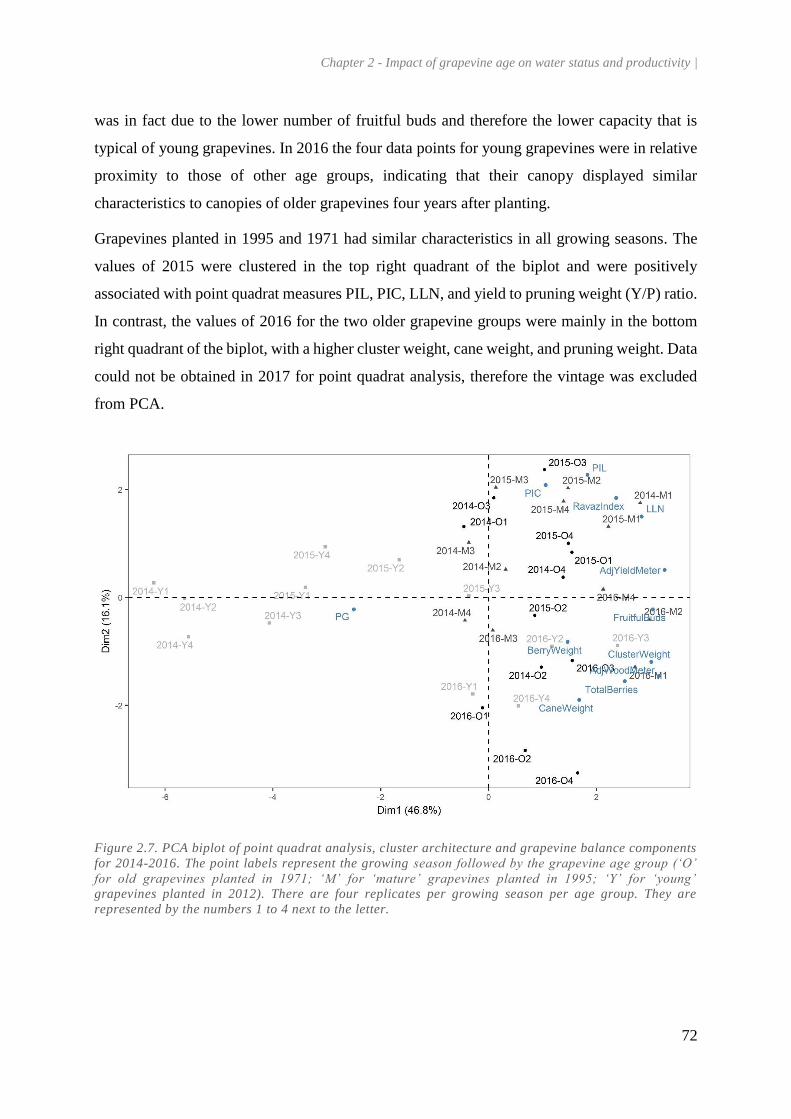
Chapter 2 - Impact of grapevine age on water status and productivity |
72
was in fact due to the lower number of fruitful buds and therefore the lower capacity that is
typical of young grapevines. In 2016 the four data points for young grapevines were in relative
proximity to those of other age groups, indicating that their canopy displayed similar
characteristics to canopies of older grapevines four years after planting.
Grapevines planted in 1995 and 1971 had similar characteristics in all growing seasons. The
values of 2015 were clustered in the top right quadrant of the biplot and were positively
associated with point quadrat measures PIL, PIC, LLN, and yield to pruning weight (Y/P) ratio.
In contrast, the values of 2016 for the two older grapevine groups were mainly in the bottom
right quadrant of the biplot, with a higher cluster weight, cane weight, and pruning weight. Data
could not be obtained in 2017 for point quadrat analysis, therefore the vintage was excluded
from PCA.
Figure 2.7. PCA biplot of point quadrat analysis, cluster architecture and grapevine balance components
for 2014-2016. The point labels represent the growing season followed by the grapevine age group (‘O’
for old grapevines planted in 1971; ‘M’ for ‘mature’ grapevines planted in 1995; ‘Y’ for ‘young’
grapevines planted in 2012). There are four replicates per growing season per age group. They are
represented by the numbers 1 to 4 next to the letter.

Chapter 2 - Impact of grapevine age on water status and productivity |
73
Table 2.3. Vine balance parameters for three age groups and four replicates over the growing seasons 2014-2017 (n = 4). Fruit yield (which includes rotten berries)
and pruning weight refer to values recorded in the field, while adjusted fruit yield and pruning weight take into account the number of missing vines per row (means
± sd).
Planting
year
% gaps
(PG)
% interior
leaves
(PIL)
% interior
clusters
(PIC)
Leaf layer
number
(LLN)
Cluster
weight (g)
Berry
number
(no./cluster)
Berry
weight (g)
Fruitful
bud
number
(buds/vine
)
Average
cane
weight (g)
Pruning
weight
(kg/m) (P)
Adjusted
pruning
weight
(kg/m)
Fruit yield
(kg/m) (Y)
Adjusted
fruit yield
(kg/m)
Yield/pr
uning
weight
(Y/P)
2014
1971 21.8 ± 7.4 25.3 ± 3.9 52.1 ± 7.41 1.61 ± 0.16 194.8 ± 72.4 144.0 ± 52.7 1.3 ± 0.15 13.4 ± 2.2 68.1 ± 9.2 0.48 ± 0.07 0.63 ± 0.13 1.31 ± 0.35 1.66 ± 0.24 2.7 ± 0.9
1995 9.5 ± 3.4 21.3 ± 5.0 50.1 ± 12.8 1.86 ± 0.34 187.4 ± 43.4 130.9 ± 26.8 1.3 ± 0.11 11.5 ± 1.3 71.8 ± 6.9 0.57 ± 0.09 0.60 ± 0.09 1.61 ± 0.16 1.70 ± 0.18 2.9 ± 0.5
2012 32.5 ± 11.2 11.5 ± 3.2 40.6 ± 11.6 1.07 ± 0.16 129.0 ± 33.8 104.7 ± 21.4 1.1 ± 0.15 7.0 ± 1.6 53.4 ± 13.2 0.27 ± 0.08 0.27 ± 0.07 0.26 ± 0.08 0.27 ± 0.08 1.0 ± 0.3
2015
1971 21.8 ± 7.4 23.6 ± 2.0 50.5 ± 6.9 1.61 ± 0.16 213.0 ± 35.0 152.6 ± 26.1 1.1 ± 0.15 13.3 ± 1.8 65.8 ± 14.6 0.43 ± 0.03 0.62 ± 0.11 1.79 ± 0.24 2.50 ± 0.13 4.1 ± 0.7
1995 19.3 ± 2.4 22.7 ± 5.6 60.4 ± 3.9 1.69 ± 0.13 208.5 ± 32.2 153.2 ± 19.7 1.1 ± 0.15 12.8 ± 1.8 61.1 ± 12.6 0.54 ± 0.11 0.56 ± 0.11 2.39 ± 0.34 2.48 ± 0.32 4.5 ± 0.5
2012 27.3 ± 11.3 17.2 ± 3.9 57.8 ± 7.8 1.41 ± 0.15 194.1 ± 48.5 153.4 ± 33.8 0.8 ± 0.18 7.8 ± 2.6 73.5 ± 17.8 0.39 ± 0.10 0.40 ± 0.09 1.00 ± 0.51 1.01 ± 0.51 2.4 ± 0.7
2016
1971 21.5 ± 6.4 13.4 ± 3.5 44.0 ± 8.0 1.40 ± 0.15 232.5 ± 49.0 172.3 ± 28.4 1.3 ± 0.16 13.5 ± 2.5 85.8 ± 18.9 0.54 ± 0.06 0.78 ± 0.06 1.27 ± 0.26 1.81 ± 0.20 2.3 ± 0.4
1995 10.0 ± 6.5 16.9 ± 2.3 49.0 ± 9.8 1.75 ± 0.24 225.6 ± 48.5 177.1 ± 41.2 1.2 ± 0.21 14.2 ± 2.3 70.4 ± 7.1 0.68 ± 0.09 0.71 ± 0.09 2.16 ± 0.45 2.23 ± 0.46 3.1 ± 0.2
2012 17.0 ± 6.9 15.2 ± 6.0 44.0 ± 5.3 1.47 ± 0.18 226.6 ± 40.6 179.8 ± 38.4 1.2 ± 0.15 11.8 ± 2.0 79.6 ± 9.4 0.66 ± 0.10 0.67 ± 0.09 2.04 ± 0.36 2.07 ± 0.33 3.1 ± 0.3
2017
1971 - - - - 209.1 ± 40.6 127.1 ± 28.5 1.6 ± 0.23 10.6 ± 2.0 99.7 ± 15.0 0.49 ± 0.08 0.71 ± 0.05 1.47 ± 0.36 2.14 ± 0.15 3.0 ± 0.4
1995 - - - - 207.2 ± 47.9 132.3 ± 24.2 1.5 ± 0.22 10.9 ± 2.2 87.2 ± 6.2 0.65 ± 0.05 0.67 ± 0.05 1.65 ± 0.25 1.69 ± 0.26 2.8 ± 0.5
2012 - - - - 174.9 ± 49.8 118.2 ± 25.0 1.4 ± 0.21 11.3 ± 2.2 70.9 ± 18.2 0.56 ± 0.14 0.57 ± 0.15 1.79 ± 0.22 1.81 ± 0.21 2.6 ± 0.6

Chapter 2 - Impact of grapevine age on water status and productivity |
74
4.5. Berry technological maturity and δ13C
Total soluble solids (TSS), titratable acidity (TA), and pH were similar for the three age group
in all growing seasons (table 2.4; appendix 2.8). However, the α-amino acid content of berries
of the youngest grapevines was more than double that of grapevines planted in 1995 and 1971
in the first and second years of the trial.
Table 2.4. Technological maturity parameters and dry mass carbon isotope discrimination (δ 13C) for the
three grapevine age groups (n = 4) over the growing seasons 2014 to 2017 (means ± sd). δ13C was only
measured in 2016 and 2017.
Planting year Total soluble
solids
(TSS; °Brix)
Titratable
acidity
(TA; g tartaric
acid L-1)
pH α-amino acids
(mg isoleucine
equivalent L-1)
δ13C (%)
2014
1971 19.33 ± 0.41 11.85 ± 1.03 2.9 ± 0.03 68.3 ± 15.65 -
1995 19.16 ± 0.65 11.31 ± 0.29 2.9 ± 0.01 66.5 ± 13.48 -
2012 19.10 ± 0.18 10.39 ± 0.62 3.0 ± 0.02 154.3 ± 12.07 -
2015
1971 20.85 ± 0.28 11.89 ± 0.25 2.9 ± 0.06 63.8 ± 16.58 -
1995 20.80 ± 0.29 12.58 ± 0.82 2.9 ± 0.03 57.0 ± 16.06 -
2012 21.30 ± 0.21 10.71 ± 0.51 3.0 ± 0.03 114.0 ± 5.94 -
2016
1971 19.56 ± 0.32 8.71 ± 1.04 3.2 ± 0.10 57.5 ± 11.67 -27.78 ± 0.13
1995 19.22 ± 0.43 8.92 ± 0.32 3.1 ± 0.04 53.0 ± 11.83 -27.03 ± 1.74
2012 18.48 ± 0.50 8.79 ± 0.73 3.1 ± 0.07 68.8 ± 11.95 -26.79 ± 1.68
2017
1971 19.73 ± 0.22 13.04 ± 0.46 3.0 ± 0.04 49.8 ± 9.64 -28.32 ± 0.34
1995 19.73 ± 0.65 12.90 ± 0.33 2.9 ± 0.02 48.8 ± 10.14 -28.26 ± 0.17
2012 20.01 ± 0.64 12.42 ± 0.38 3.0 ± 0.03 53 ± 9.13 -28.02 ± 0.69
The δ13C analysis that took place in 2016 and 2017 on mature berries indicated only a weak
water deficit during both growing seasons. No significant differences were recorded among age
groups (P = 0.31).
4.6. Experiment on water deficit
In the framework of the water deficit trial on cordon vines, the soil water content measured at
flowering and pea-sized berries in 2016 was approximately 5% lower for the stressed treatment
compared to the control for all age groups (figure 2.8; appendix 2.9). However, due to the dry

Chapter 2 - Impact of grapevine age on water status and productivity |
75
weather around veraison and the lack of covering, the soil water content of stress and control
treatments tended to converge at the end of the season, especially in the lowest soil horizon.
The frequency and intensity of precipitation events in the first half of the 2017 season led to
similar water content for all treatments between flowering and pea-size, but not when measured
two weeks after veraison (0 - 30 cm: Year, P < 0.001; Water status, P < 0.001; Year × Water
status, P = 0.038. 30-60 cm: Year, P < 0.001; Water status, P < 0.001; Year × Water status, P
= 0.54). There were no differences in leaf chlorophyll between age groups in 2016 and 2017
(figure 2.9), as well as no differences between years and water treatments. The stomatal
conductance measured on cordon vines in 2016 and 2017 showed significant differences across
vine age groups (P < 0.001; figure 2.10). The water treatment also affected grapevine response,
but its effect depended on the year (Year × Water status, P = 0.039).
Over most of the 2017 season vines planted in 2012 and subjected to water deficit had the
lowest stomatal conductance. During this season, the high precipitations combined with the
vineyard slope led to water runoff, which affected upper and lower blocks to different extents
and increased spatial heterogeneity. ΨPD on cordon vines decreased along the 2016 growing
season for the cordon vines of all age groups and treatments, with the lowest ΨPD being observed
for vines planted in 2012 towards harvest (figure 2.11). Values above -0.4 MPa were maintained
over the 2017 growing season for all vine ages and treatments, and only the vines planted in
2012 under the stress treatment showed mild water stress around -0.3 MPa, which is usually
defined as the limit for the onset of water stress for white cultivars (Schultz and Matthews,
1988).

Chapter 2 - Impact of grapevine age on water status and productivity |
76
Figure 2.8. Soil water content for the water deficit experiment on cordon vines in 2016 and 2017 at
flowering, pea-sized berries, and two weeks after veraison (means ± sd) at horizons 0-30 cm and 30-60
cm.
Figure 2.9. Chlorophyll fluorescence ratio under green excitation (SFR_G) measured at regular time
intervals on selected cordon vines for the water deficit experiment from flowering to harvest in 2016 and
2017 (means ± sd).

Chapter 2 - Impact of grapevine age on water status and productivity |
77
Figure 2.10. Stomatal conductance (gs) measured periodically on selected cordon vines for the water
deficit experiment over the growing seasons of 2016 and 2017 (means ± sd).
Figure 2.11. Predawn water potential (ΨPD) measured on cordon-trained vines for the water deficit
experiment over the growing seasons of 2016 and 2017 (means ± sd).
The δ13C of cordon vines was affected by age (P < 0.001) and year (P < 0.001) but not by water
treatment (P = 0.31). This variable mirrored the trend observed for ΨPD in 2017. Nevertheless,
neither planting year, season, nor water status were sufficiently different to warrant definitive
conclusions (table 2.5).
Table 2.5. Dry mass carbon isotope discrimination (δ13C) measured at mature berries on cordon vines for
the water deficit experiment over the growing seasons of 2016 and 2017 (means ± sd).

Chapter 2 - Impact of grapevine age on water status and productivity |
78
Planting year Water deficit experiment (single cordon)
δ13C – Control (%) δ13C – Stress (%)
2016
1971 -27.54 ± 0.33 -27.97 ± 0.41
1995 -27.68 ± 0.13 -27.74 ± 0.28
2012 -26.02 ± 1.19 -25.66 ± 1.64
2017
1971 -28.23 ± 0.69 -28.27 ± 0.71
1995 -28.94 ± 0.19 -28.56 ± 0.53
2012 -28.25 ± 0.54 -26.81 ± 2.16
5. Discussion
The present work is unique in that it compares field-grown vines of different planting years but
identical genetic material in a single experimental vineyard. It is also, to the authors’ knowledge,
the only study to compare three vine groups with age gaps of around 20 years in the same
environmental conditions: starting from two year old vines in their first productive vintage,
nineteen year old vines representative of ‘mature’ vineyards, and forty-three year old vines that
are reasonably considered as ‘old vines’ in the public opinion (Historic Vineyard Society, 2018).
Studying three age groups simultaneously can provide insight about the timing at which
changes occur in vine physiology and productivity. However, a long-term trial such as this one
was bound to be influenced by external factors, and vine decline was the most important. The
decision was made early on not to replace dying or missing vines over time, as it would have
led to increasing heterogeneity in row populations. Instead, special care was taken when
selecting vines for seasonal measurements. The main purpose of the selection was to avoid
vines adjacent to missing spaces and detect extreme outliers while confirming the health status
of the selected vines. Despite precautions, two selected vines were tested as positive for viral
infections in 2017, even though their general response was not markedly affected during the
trial.
Another factor of influence was the cover crop. The Rheingau region is generally described as
a cool wine region, with lower GDD accumulation and frequent precipitations over the growing
season (Gladstones, 2011). Winegrowers have traditionally adapted to the constraints of this
climate by preferring rootstocks that restrict scion vigor (Reynolds, 2015). Cover crops are
frequently used as a complementary lever to manage vegetative growth due to their ability to

Chapter 2 - Impact of grapevine age on water status and productivity |
79
reduce the availability of water and nutrients, especially nitrogen, in upper soil layers (Agnelli
et al., 2014; Celette et al., 2008). In order to prevent excessive competition with the youngest
vines, the introduction of cover crop in newly established rows was postponed to the third year
after planting for all vines. This treatment was applied to the entire vineyard when it was
established in 1971 and for newly planted rows in 1995 and 2012. Nitrogen supplied from the
soil contributes directly to berry development and has been positively correlated with yeast-
assimilable nitrogen (YAN) content in must (Bell and Henschke, 2005). However, excessive
nitrogen promotes vegetative growth, which can lead to dense canopies with low light
interception and temperature and higher humidity. Such conditions are optimal for the
development of fungal pathogens like Botrytis cinerea that can severely reduce grape quality
and yield (Percival et al., 1994). Shaded canopies also tend to decrease the vine’s water use
efficiency (WUE) since inner leaves marginally contribute to photosynthesis but still transpire
(Keller et al., 2016). The presence of cover crop in 2016 and 2017 reduced the soil water content
for vines planted in 2012, reaching values in line with rows planted in 1995 and 1971 at both
0-30 cm and 30-60 cm horizons.
Stomatal closure is among the earliest physiological responses to water deficit, followed by a
decrease in photosynthesis and transpiration (Chaves et al., 2010; Loveys et al., 2004). In the
relatively warm growing season of 2016, these variables were consistently lower for double
Guyot vines planted in 2012, with no apparent differences between vines planted in 1995 and
1971. In 2017, a year characterized by frequent precipitation events during the season, vines
planted in 2012 had a similar response to older vine groups.
Because assimilation, stomatal conductance and transpiration were measured on leaves, these
parameters were representative of WUE at leaf level and were dependent on leaf environment
at the time of measurement (Tomás et al., 2014). On the other hand, δ13C is well correlated with
midday stem water potential (Gaudillère et al., 2002; van Leeuwen et al., 2009) and provides
an integrated assessment of the whole-vine response to water deficit when measured in berry
juice at harvest (Bchir et al., 2016). Vine age did not significantly impact δ13C over 2016 and
2017, but the measurements underlined seasonal variation.
Vine productivity is often discussed in reference to vine capacity and vine balance. The term
‘vine capacity’ is used to describe the maximal productivity of a grapevine (Howell, 2001)
while ‘vine balance’ is expressed as the equilibrium between vegetative growth and crop level

Chapter 2 - Impact of grapevine age on water status and productivity |
80
leading to optimal fruit quality (Gladstones, 1992). An insufficient leaf area will fail to fully
ripen a crop, while excessive shoot growth affects canopy microclimate by altering light
exposure, temperature, and humidity inside the canopy (Smart and Robinson, 1991). Previous
studies have reported that pruning weights above 1.0 kg m-1 are generally detrimental to fruit
quality, while optimal values varied between 0.3 to 0.6 kg m-1 depending on plant material and
field conditions (Dry et al., 2004). Another common measure for vine balance is pruning weight
ratio (Y/P) with an optimal range estimated between 4 and 10(Dry et al., 2004). Ratios under 4
are often associated with excessive vigor, but they can be still be considered optimal in cool
climates to compensate for lower ambient light and temperature (Kliewer and Dokoozlian,
2005).
In the present trial, even though the youngest vines had access to higher amounts of nitrogen in
the first years after planting, their low bud fruitfulness had a larger impact on their canopy
architecture, as shown by their high PG and low PIL, PIC, and LLN (table 3). The reduced bud
count of these vines in 2014 and 2015 also translated into low pruning weight and yield. The
capacity of vines planted in 2012 increased over time to become comparable to other groups in
2016 (figure 2.7), with their Y/P ratio increasing from 1.0 to 3.1 in the same period. Overall,
the productivity of vines planted in 1995 and 1971 was more difficult to assess due to missing
and symptomatic vines. In 2015, 27% of the vines originally planted in 1971 had already ceased
production, compared to only 2% for vines planted in 1995 (table 4). In 2016, the oldest vines
had the lowest recorded yield among age groups, but once adjusted to account for missing vines
their yield was similar to vines planted in 2012 and 1995.
Trunk diseases such as esca, caused by complexes of xylem-dwelling fungi (Bertsch et al., 2013;
Mugnai et al., 1999), can dramatically hinder canopy and yield formation. Esca specifically is
becoming a widespread threat for vineyard longevity (Larignon et al., 2009). The disease
precipitates vine decline and leads to apoplexy, with leaf fall and berry shriveling on shoots,
and ultimately to vine death (Bertsch et al., 2013). Trunk diseases are chronic issues in old
vineyards. Their cumulated incidence often correlates linearly with the age the vineyard (Surico
et al., 2006), and they appeared as an inevitable constraint in this trail. The decision not to
replace dying or missing vines by co-plantation meant that the remaining plants would be facing
less competition and display higher vegetative and reproductive productivity, as noted in
experiments that varied planting density (Bernizzoni et al., 2009). Some caution should be

Chapter 2 - Impact of grapevine age on water status and productivity |
81
applied when reviewing this data since it is possible that vines planted in 1971 could have been
less productive if all vines were present.
Nevertheless, most results obtained for the main trial on double Guyot vines were in agreement
with previous research that described young vines as being more sensitive to water deficit
(Zufferey and Maigre, 2007), but no differences among technological maturity parameters were
noted other than the high α-amino acid content of the youngest vines in the absence of cover
crop.
The water deficit experiment on cordon vines gave results similar to the double Guyot vines.
The success of this secondary trial was based on the duration and intensity of precipitation
events, which varied across growing seasons. The trial was considered in 2016 after sowing the
cover crop, but its implementation in double Guyot rows was not possible due to the relatively
small size of the vineyard and the inevitable interference that the plastic sheets would have with
selected vines. It was therefore decided to use the adjacent cordon rows that were managed in
the same way as the double Guyot rows with the addition of the water treatment (control or
stress) used as a fixed LMM effect. The plastic sheets that were deployed during rain events
were able to create a difference in soil moisture between stressed and control treatments at 0-
30 and 30-60 cm, and this was reasonably visible in gs and ΨPD measurements. A distinction
between control and stressed vines was gradually settling over the 2016 growing season, but
the high temperatures and absence of rain towards harvest reduced differences based on water
treatment, and the three vine age groups followed the same patterns as double Guyot vines. In
2017, it was only possible to obtain differences between stress and control treatments for the
youngest vines. This was relatively supported by δ13C measurements, with young stressed vines
reaching -26.81% on average. In order to confirm the 2016 results on water deficit, it may have
been desirable to increase the coverage area and/or the number of measured vines per treatment
to reduce the impact of water runoff along the vineyard slope, which was responsible for
increased differences between blocks. Yet, the fact that the youngest vines in both control and
stress treatments experienced water stress in 2016, while only the youngest vines under the
stress treatment differed from other groups in 2017, suggests that the smaller exploration of
their root system is indeed the driving factor behind the youngest vines’ lower tolerance to
water deficit (Zufferey and Maigre, 2007).
Chapter 2 - Impact of grapevine age on water status and productivity |
82
The study underlines the special considerations needed during the establishment of young vines,
as well as the ability possibility to maintain vineyards with a long-term perspective if diseases
are prevented. This would create compounded benefits terms of adaptability to water deficit
and yield conservation. Vine size and capacity were determinant factors in the youngest vines’
productivity (Grigg et al., 2017), which gradually increased from the first to the fourth years
after planting.
Future research will focus on the analysis of secondary metabolites in juice and berry skins, as
well as chemical and sensory analysis of wines obtained from the three grapevine groups. It
will also be interesting to study the evolution of carbohydrate reserves and root density as vines
become older to learn more about the interaction of these factors with the vine’s response to
water deficit and its productivity.
6. Conclusion
In the present work we examined the physiological behavior, productivity, and berry
technological maturity of vines planted in the same vineyard in 1971, 1995, and 2012.
Photosynthesis, stomatal conductance, and transpiration were generally lower for the youngest
vines, even though their response was dependent on seasonal factors. One can speculate that
given our results, a possible explanation is that the shallower root system of young vines and
its proximity to soil surface, may prevent access to deeper water reserves in periods of drought.
The youngest vines also displayed smaller canopy size and lower productivity than older groups
at the beginning of the study. However, they were able to reach similar levels of bud fruitfulness,
yield, and pruning weight in the fourth years after planting. The behavior of vines planted in
1971 and 1995 did not differ for most vegetative and generative parameters including water
status, canopy architecture, cluster parameters, and technological maturity. The most
distinguishing factor between the two older groups was the higher incidence of trunk diseases
for vines planted in 1971, which resulted in a non-negligible decrease in recorded yield despite
the fact that individual vine production was similar among the two groups.
The results of this study indicate that provided they are managed in the same way, the
physiological behavior, productivity, and berry composition of individual vines around 20 and
40 years old and planted in conditions of cool climate and deep soil is comparable, with yield
decline being mostly due to trunk diseases.

Chapter 2 - Impact of grapevine age on water status and productivity |
83
7. Acknowledgments
The authors gratefully acknowledge the support of Dr. Susanne Tittmann, Magali Blank and
Bernhard Gaubatz (Department of General and Organic Viticulture, HGU) for laboratory
organization and vineyard management, Stefan Muskat and Ralf Lehnart for soil sampling and
analysis (Department of Soil Sciences and Plant Nutrition, HGU) as well as Dr. Elvira Bleser
and Johannes Kiesgen (Department of Grapevine Breeding, HGU) for performing the ELISA
tests. Carbon isotope discrimination was made by Olivier Mathieu of the joint research unit
Biogeosciences (CNRS/University of Burgundy). The authors would also like to thank the
students Julian Dittmann, Hélène Georges, Elise Laizé, Maximilian Pfahl, and Liying Shao for
their contribution to data collection.
8. Funding
This work was funded by a doctoral scholarship to Khalil Bou Nader from the “Forschungsring
des Deutschen Weinbaus” (FDW) association.

Chapter 3. Impact of grapevine age
on berry structure and secondary
metabolites
This chapter is in preparation for publication in a modified version as:
Bou Nader, Khalil, Eric Gomès, Ghislaine Hilbert, Christel Renaud, Jean-Philippe Roby, Serge
Delrot, Hans R. Schultz, et al. “A Bottle of Old Vines Part 1. The Impact of Vine Age on
Riesling Berry Structure and Composition.” American Journal of Enology and Viticulture.
Author contributions: the author designed and conducted the research experiments, analyzed the
data, drafted and constructed the manuscript. Free and potential monoterpene and norisoprenoid
analysis was performed by Stefanie Fritsch (Department of Microbiology and Biochemistry,
HGU).

Chapter 3 - Impact of grapevine age on berry structure and secondary metabolites |
85
1. Introduction
There seems to be a general consensus about the ability of old grapevines to produce wines of
superior character (Goode, 2005; Heymann and Noble, 1987; Koblet and Perret, 1982; Zufferey
and Maigre, 2008), possibly due to larger wood reserves (Howell, 2001) or to an improved
equilibrium between vegetative growth and yield (Zufferey and Maigre, 2008).
Previous research on grapevine age has examined berry composition of young and old vines,
however most studies only focused on primary metabolites and technological maturity
indicators (Grigg et al., 2017; Reynolds et al., 2008; Zufferey and Maigre, 2008). Some studies
reported that old grapevine berries had a higher titratable acidity and formol index than young
grapevines, while sugar content was not markedly different among grapevine age groups
(Zufferey and Maigre, 2007). However, the observed trends appeared to be strongly dependent
on weather conditions during the growing season, as well as vineyard location (Grigg et al.,
2017; Reynolds et al., 2008).
Climate is usually a better predictor of overall grape quality than soil characteristics (van
Leeuwen et al., 2004). However, the concentration of soil organic matter can still affect berry
parameters, whether directly by increasing nitrogen supply to the berries, or indirectly by
favoring vegetative growth (Habran et al., 2016). Canopy density is known to affect berry
quality by having a direct impact on cluster light exposure, temperature, and humidity (Smart
and Robinson, 1991). Vigorous grapevines with dense canopies show a tendency to have higher
humidity and shade and lower temperatures in the cluster zone. This not only promotes fungal
infections (Austin et al., 2009) but also affects berry composition and quality (Dry et al., 2004).
The compounds that are affected by canopy density include aromatic compounds such as
monoterpenes, norisoprenoids as well as skin flavonols, especially for white cultivars.
Monoterpenes have been associated with the aroma profile of Muscat varieties and non-Muscat
aromatic varieties such as Gewürztraminer and Riesling (Mateo and Jimenez 2000). They are
mostly present in berries as glycosidic conjugates and are gradually released during wine
fermentation and aging (Black 2015). Thin canopies have also been shown to increase the
expression of the terpene synthase genes and as a result the berry monoterpene content due to
the higher sun exposure of clusters (Friedel et al., 2016; Skinkis et al., 2010).
Norisoprenoids are formed from the degradation of carotenoids in berry skin after they undergo
chemical, photochemical, and/or oxidative reactions (Robinson et al., 2014). As such, these

Chapter 3 - Impact of grapevine age on berry structure and secondary metabolites |
86
reactions are highly impacted by temperature and light. Marais et al. (1999) have demonstrated
early on that artificially shaded canopies, which received less light and had lower temperatures
during the season, produced lower concentrations of norisoprenoids compared to control
grapevines.
Flavonols are phenolic compounds located in berry skin that act as protectants against oxidation
by UV radiation (Haselgrove et al., 2000). Light exposure positively impacts grape flavonols,
especially quercetin glucosides (Cortell and Kennedy, 2006; Friedel et al., 2015). The effects
of temperature and light are inherently difficult to separate in field experiments. Nevertheless,
studies that have focused on vineyard orientation (Friedel et al., 2016) or have artificially cooled
sun-exposed clusters reported that high temperatures inhibits the production of phenolic
compounds such as anthocyanins without having an impact on flavonols (Spayd et al., 2002).
In order to examine the potential effects of grapevine age berry structure and composition, a
vineyard planted in Geisenheim, Germany, with alternating rows of Riesling grapevines on
identical rootstock that were planted in 1971, 1995 and 2012, was studied from 2014 to 2017
(Bou Nader et al., 2019). Riesling is usually described as a non-Muscat white aromatic cultivar,
with a wine profile heavily influenced by monoterpenes and norisoprenoids (Günata et al., 1985;
Lott et al., 2010). The two classes of compounds contribute in large part to the cultivar’s typical
floral and fruity aromas, in addition to its well-recognized ‘kerosene’ aroma due to the presence
of free 1,1,6-trimethyl-1,2-dihydronaphthalene (TDN) (Mateo and Jiménez, 2000).
The aim of this work was to compare the three grapevine age groups with regards to their berry
composition, with a focus on amino acids, free and potential monoterpenes and norisoprenoids,
and flavonols to examine whether the nature and concentration of these compounds were
affected by grapevine age.
2. Materials and methods
2.1. Experimental design and plant material
A single experimental plot located in Geisenheim, Germany, with alternating rows of Vitis
vinifera (L.) cv. Riesling grapevines (clone Gm 239-17) on 5C Teleki rootstocks and trained in
double Guyot was studied. While the vineyard was planted in 1971, some rows were uprooted
in 1995 and 2012 and replanted with the same plant material in order to obtain four blocks with
each grapevine age group. The vineyard is described in more detail in Bou Nader et al. (2019).

Chapter 3 - Impact of grapevine age on berry structure and secondary metabolites |
87
It was studied from 2014, which was the first year of harvest for grapevines planted in 2012,
until 2017.
Due to the general vigor of the site, a cover crop of grass and clover was sown in alternating
rows (Bou Nader et al., 2019). When the second group of grapevines was planted in 1995, their
rows were ploughed in the first two years to prevent excessive competition with the cover crop
during the early developmental stages of the grapevines (Williams et al., 1990). The same
treatment was applied from 2012 to 2014 in the rows of young grapevines. Afterwards, these
rows were sown with the same cover crop combination that already existed in 1995 and 1971
rows. Soil nitrate and water content from depths of 0 to 30 cm and from 30 to 60 cm were
significantly higher in 2014 and 2015 for rows planted in 2012, but after this period the three
age groups had similar soil nitrate and water contents (Bou Nader et al., 2019).
2.2. Berry sampling
Phenology was followed with the modified E-L system developed by Coombe (1995). No
significant phenological shifts were found between grapevine age groups during the study.
Veraison date was determined by the onset of berry softening and the beginning of soluble solid
accumulation. Before harvest date, which was decided according to technological maturity and
berry health status, randomized samples of 40 berries were collected for each treatment ×
replicate combination for a total of 12 samples (n = 4). The berries were collected by cutting
their pedicel with scissors and placed in plastic boxes that were saturated with CO2. This was
done to limit oxidation during storage. The samples were then placed in a freezer at -20 °C.
Berries were taken out of the freezer one by one and peeled while still frozen. The pedicel, skin,
seeds, and pulp were separated and weighted. The skins and seeds were returned to the freezer
while the pulp was pressed in a plastic bag to extract the juice. The juice was centrifuged for
3 min at 4500 g at room temperature. Aliquots for organic acids analysis were diluted with
ultrapure water from a quarter to a tenth depending on the stage of maturity before bieng frozen
in order to prevent tartaric acid precipitation during storage.
The skins were freeze-dried for 5 days in an Alpha1-4 freeze-dryer (Martin Christ
Gefriertrocknungsanlagen GmbH, Osterode am Harz, Germany) and were weighed to
determine their dry weight. The samples were then ground with the MM200 mixer mill (Retsch
GmbH, Haan, Germany) for 30 seconds at a vibrational frequency of 25 s-1 to obtain a fine
powder.
Chapter 3 - Impact of grapevine age on berry structure and secondary metabolites |
88
Berry samplings for the analysis of potentially volatile monoterpene and were collected on the
same dates as other berry samplings. In this case, 200 berries per replicate were collected with
their pedicel and placed in liquid nitrogen under CO2 atmosphere. The samples were then stored
at -20 °C in sealed bags including CO2 until analysis.
2.3. Organic and amino acids
Tartaric and malic acid concentrations were quantified with a TRAACS 800 continuous flux
analyzer (Bran & Luebbe, Plaisir, France) and the AACE AutoAnalyzer software (Bran &
Luebbe, Plaisir, France). It allowed measuring malic acid titration using the enzymatic
spectrophotometric method at 340 nm after the reduction of NAD+ to NADH by malate
dehydrogenase (Merck, Darmstadt, Germany). Tartaric acid content was determined by
colorimetry at 520 nm after reacting with ammonium vanadate in the presence of 2 g L-1 NaOH
to form the metapervanadyl tartrate complex (Torres et al., 2017).
Free amino acids in must were derived according to Hilbert et al. (2003) modified by Habran
et al. (2016). The derivatization reagent was 6-aminoquinolyl-N-hydroxisuccinimidyl
carbamate (AccQ-Tag, supplied by Waters, Milford, MA USA). Samples were then analyzed
on an UltiMate 3000 ultra-high performance liquid chromatography (UHPLC) system with a
FLD-3000 fluorescence detector (Thermo Electron SAS, Waltham, MA USA). The separation
occurred at 37 °C in an AccQ-Tag Ultra column of dimensions 2.1 × 100 nm and particle size
1.7 μm (Waters, Milford, MA USA). Elution rate was maintained at 0.5 mL min-1 with the
following elution gradient (v/v): 0 min 93% A 4.2% B 2.8% C, 6.5 min 95% A 8.4% B 5.6%
C, 9 min 78% A 13.2% B 8.8% C, 11 min 71% A 17.4% B 11.6% C linear for 2 min, 14 min
60% B 40% C linear for 1 min, 15 min 93% A 4.2% B 2.8% C (eluent A, sodium acetate buffer,
140 mM at pH 5.7; eluent B, acetonitrile 100%; eluent C, ultrapure water). An ultrapure water
control was added before each set of 18 samples ensure retention time and baseline consistency.
Standard samples containing 20 amino-acids (Alanine, Arginine, Aspartic acid, Asparagine,
Cysteine, GABA, Glycine, Glutamic acid, Glutamine, Histidine, Isoleucine, Leucine, Lysine,
Methionine, Phenylalanine, Proline, Serine, Threonine, Tyrosine, Valine) were used as external
standards to calibrate amino-acid quantification (Sigma, St Louis, MO USA). Chromatograms
were recorded for excitation at 250 nm and emission at 395 nm. The software Chromeleon 7.1
(Thermo Electron SAS, Waltham, MA USA) was used to calculate peak area.

Chapter 3 - Impact of grapevine age on berry structure and secondary metabolites |
89
Must sugar content was measured by enzymatic titration using a Glucose/Fructose enzymatic
kit (BioSenTec, Toulouse, France). Samples were diluted with a Precision 2000 microplate
preparation robot (Biotek Instruments Inc., Winooski, VT, USA) and analyzed with an
ELx8000UC microplate reader (Biotek Instruments Inc., Winooski, VT, USA) by tracking the
change of absorbance at 340 nm.
2.4. Potentially volatile monoterpenes and C13-norisoprenoids
Potentially volatile monoterpenes and C13-norisoprenoids were analyzed by a modified solid-
phase extraction (SPE) for sample preparation (Günata et al., 1985) as described in Schüttler
(2012) and (Schüttler et al., 2015), followed by gas chromatography coupled with mass
spectrometry (GC-MS). The method was adapted by replacing the enzymatic release of
aglycones by acid hydrolysis using the procedure described by (Kotseridis et al., 1999).
Frozen berry samples were allowed to thaw overnight at 4 °C and were blended with a
household blender for 30 s. The resulting must was distributed in 50 mL falcon tubes (VWR,
Lutterworth, UK) and centrifuged three times at 7200 g and 4 °C in a 5430 R centrifuge
(Eppendorf, Hamburg, Germany) and the clear must was analyzed.
Strata SDB-L cartridges containing 500 mg of styrene-divenylbenzene polymer (Phenomenex,
Torrance, CA USA) were preconditioned with 5 mL of pentane/dichloromethane (2/1 v/v),
followed by 10 mL of methanol, 10 mL of methanol/H2O (1/1 v/v) and 10 mL of H2O. Must
samples of 50 mL were diluted 1:1 with ultrapure water and were spiked with octan-3-ol and
2.6-dimethylhept-5-en-2-ol (DMH) as internal standards (c(octan-3-ol) = 50 µg L-1; c(DMH) = 25 µg
L-1) and were loaded on the SPE cartridges. Cartridges were washed again with 10 mL of water
and dried for 1h with nitrogen under vacuum (see above). Dried samples were eluted with 10
mL of pentane/dichloromethane (2/1 v/v). The eluates were dried with anhydrous sodium
sulfate and concentrated to a final volume of 50 µL under gentle nitrogen flow, and 2 µL were
used to analyze free monoterpenes and norisoprenoids by gas chromatography.
For potentially volatile monoterpenes and norisoprenoids the SPE cartridges were eluted with
10 mL of ethyl acetate. The fractions were evaporated to dryness under vacuum with a rotary
evaporator (Büchi, Flawil, Switzerland) at water bath temperature 40 °C and p = 138 kPa. The
residues were resolved in 5 mL of 0.2 M citric acid (pH = 2.5), transferred to 10 mL head space
vials, sealed, and heated in a laboratory oven at 100 °C for 60 min. After cooling down the
samples on ice, the internal standard mix was added based on the initial sample volume. Three
Chapter 3 - Impact of grapevine age on berry structure and secondary metabolites |
90
successive liquid-liquid extractions were conducted with 2 mL, 1 mL, and 1 mL
pentane/dichloromethane (2/1 v/v), combined with anhydrous sodium sulfate and concentrated
under nitrogen flow to a final volume of 50 µL. Gas chromatography coupled to mass
spectrometry (GC-MS) was performed with a Thermo Fisher Trace GC Ultra gas
chromatograph equipped with a PTV injector and coupled to a Thermo Fisher ITQ 900 Ion Trap
MS mass spectrometric detector (Thermo Fisher Scientific, Waltham, MA USA). Samples (2
µl) were injected in spitless mode (spitless time 90 s) at 200 °C. An Agilent DB-Wax capillary
column of dimensions 30 m × 0.25 mm ID × 0.5 µm film density (Agilent Technologies, Santa
Clara, CA, USA) was used for the separation. The following temperature gradient program was
used: 40 °C for 1 min, then temperature increased until 60 °C at 10 °C min-1, then from 60 °C
to 200 °C at 3 °C min-1, and from 200 °C to 230 °C at 10 °C min-1. The temperature was finally
maintained at 230 °C for 10 min. Helium was used as a carrier gas with a flow rate of 1.4 mL
min-1 and average velocity of 27 cm s-1. The interface and MS source temperatures were set to
240 °C and 200 °C respectively. Mass spectrometric data was acquired in electron impact mode
(EI) with an ionization energy of 70 eV. Quantification was made with the Selected Ion
Monitoring (SIM) mode.
2.5. Flavonol content in berry skin
The flavonol extraction from skins was done according to Hilbert et al. (2015) with 20 mg of
skin powder per sample and 500 μl of acidified methanol at 0.1% HCl (v/v). The extracts were
centrifuged for 1 min at 4500 g and were filtered directly in UHPLC vials with 0.22 μm syringe
filters (GHP Acrodisc, Pall Gelman Corporation, Ann Arbor, MI, USA). The analysis was
performed as described by Torres et al. (2017) with an UltiMate 3000 UHPLC system (Thermo
Electron SAS, Waltham, MA USA) equipped with a DAD-3000 diode array detector at a
wavelength of 360 nm (Thermo Electron SAS, Waltham, MA USA). The separation was made
with a Syncronis C18 column of dimensions 2.1 × 100 mm and particle size 1.7 μm (Thermo
Fischer Scientific, Waltham, MA USA) at an elution debit of 0.368 mL min-1 and the following
binary gradient (v/v): 0 min 92.2% A 7.8% B, 9.6 min 73% A 27% B, 14.1 min 70% A 30% B,
14.8 min 92.2% A 7.8% B (eluent A,ultrapure water and formic acid, 90/10 v/v; eluent B,
acetonitrile 100%). The retention times and UV-visible spectrometric data of the samples were
compared with those of pure standards for the identification and assignment of peaks. Peak area
was calculated with the Chromeleon 7.1 software (Thermo Electron SAS, Waltham, MA, USA).
Chapter 3 - Impact of grapevine age on berry structure and secondary metabolites |
91
Individual flavonol concentrations were translated in milligrams per gram (mg g-1) of dry skin
with quercetin-3-O-glucoside (Extrasynthèse, Genay, France) as reference.
2.6. Statistical analysis
The statistical analysis was performed with RStudio (version 1.1.453; Rstudio, 2018) and R
(version 3.5.0; R Core Team, 2018). Linear mixed-effect models (LMM) were used to evaluate
the effect of grapevine age on the parameters of interest. Grapevine age and year were converted
to categorical variables and used as fixed effects in all models and field replicates were added
as random effects. Model parameters were estimated by restricted maximum likelihood (REML)
with the packages lme4 (Bates et al., 2015) and pkbrtest (Halekoh and Højsgaard, 2014). The
importance of fixed effects was assessed by Kenward-Roger approximations at a significance
level of P = 0.05 (Schaalje et al., 2002). Graphics were drawn with the ggplot2 package (version
2.2.1; Wickham, 2009).
Principal Component Analysis (PCA) was used to examine the various classes of chemical
compounds measured in berry skin and juice. For this analysis, the current dataset was
combined with data about technological maturity parameters (average berry weight, must
titratable acidity, pH, total soluble solids, and α-amino acids) described in Bou Nader et al.
(2019) (see Chapter 2).The scaled berry composition data was also assessed by k-means
clustering with 50 iterations to reach convergence (Hartigan and Wong, 1979). Four clusters
were used based on agreement between the gap statistic and elbow methods.
PCA and k-means clustering were executed with the packages FactoMineR (version 1.41; Lê
et al., 2008) and factoextra (version 1.0.5; Kassambara and Mundt, 2017). The point labels
represent the growing season followed by the grapevine age group (‘O’ for ‘old’ grapevines
planted in 1971; ‘M’ for ‘mature’ grapevines planted in 1995; ‘Y’ for ‘young’ grapevines
planted in 2012). There are four replicates per growing season per age group. They are
represented by the numbers 1 to 4 next to the letter.
3. Results and discussion
3.1. Berry composition
Due to the absence of cover crop in rows planted in 2012 during the growing seasons 2014 and
2015 (Bou Nader et al., 2019), the concentration of various amino acids in must was higher for
the youngest grapevine age group, especially in 2015 (table 3.1). Notably, the amino acids most
present in the berries from 2012 grapevines in 2015 were α-ketoglutarate derivatives glutamine,
Chapter 3 - Impact of grapevine age on berry structure and secondary metabolites |
92
arginine, and proline, as well as phenylalanine. Glucose, fructose, malic and tartaric acid
concentrations were similar for the three age groups but were susceptible to yearly changes.
Free and potentially volatile monoterpenes and norisoprenoids also showed a similar trend
(table 3.2), with a potential TDN content of 8.8 μg L-1 for grapevines planted in 2012 compared
to 4.6 and 3.3 μg L-1 for grapevines planted in 1995 and 1971, respectively. The concentrations
of the studied flavonols were dependent on the season, with higher values in 2017 for all age
groups. This may be due to the partial defoliation that took place at fruitset as already reported
(Mijowska et al., 2016; Yu et al., 2016).
The PCA showed a clear separation between data points of 2015 and those of 2016 and 2017
(figure 3.1). Young grapevines were highly represented by α-amino acid content and individual
amino acids in 2015, especially phenyalanine (figure 3.2; appendix 3.1). In 2016 only one
replicate of grapevines planted in 2012 had higher amino acid concentration. Interestingly
phenylalanine content in juice was inversely proportional with quercetin-3-galactoside and
quercetin-3-glucuronide, but this correlation is not sufficient to draw a direct connection to the
phenylpropanoid pathway, in which phenylalanine is used as a substrate to produce flavonoids
(Flamini et al., 2013; Yin et al., 2012). As mentioned for the α-amino acid content, soil
ploughing and the absence of cover crop in 2015 for grapevines planted in 2012 were most
likely responsible for the high increase in their berry amino acid content (Giese et al., 2015). A
higher nitrogen content in berries is also known to favor the production of monoterpenes and
some norisoprenoids (Linsenmeier and Löhnertz, 2016).
Young grapevines tend to be more sensitive to water stress (Bou Nader et al., 2019; Zufferey
and Maigre, 2007). Seasonal water deficit may also affect monoterpene and norisoprenoid
concentration (Deluc et al., 2009). In an experiment on partial rootzone drying, Bindon et al.
(2007) showed that moderate water stress decreased berry weight at harvest and increased the
production of norisoprenoids. The influence of water stress on berry flavonols depends on its
intensity and its timing during the growing season, with post-veraion water deficits having only
limited impact on flavonol content (Torres et al., 2017). In the present trial, grapevines planted
in 2012 experienced a weak water stress at the end of the 2015 and 2016 growing seasons (Bou
Nader et al., 2019). Therefore it is difficult to clearly differentiate between the effects of
nitrogen and water status on the berry composition of the youngest grapevines.
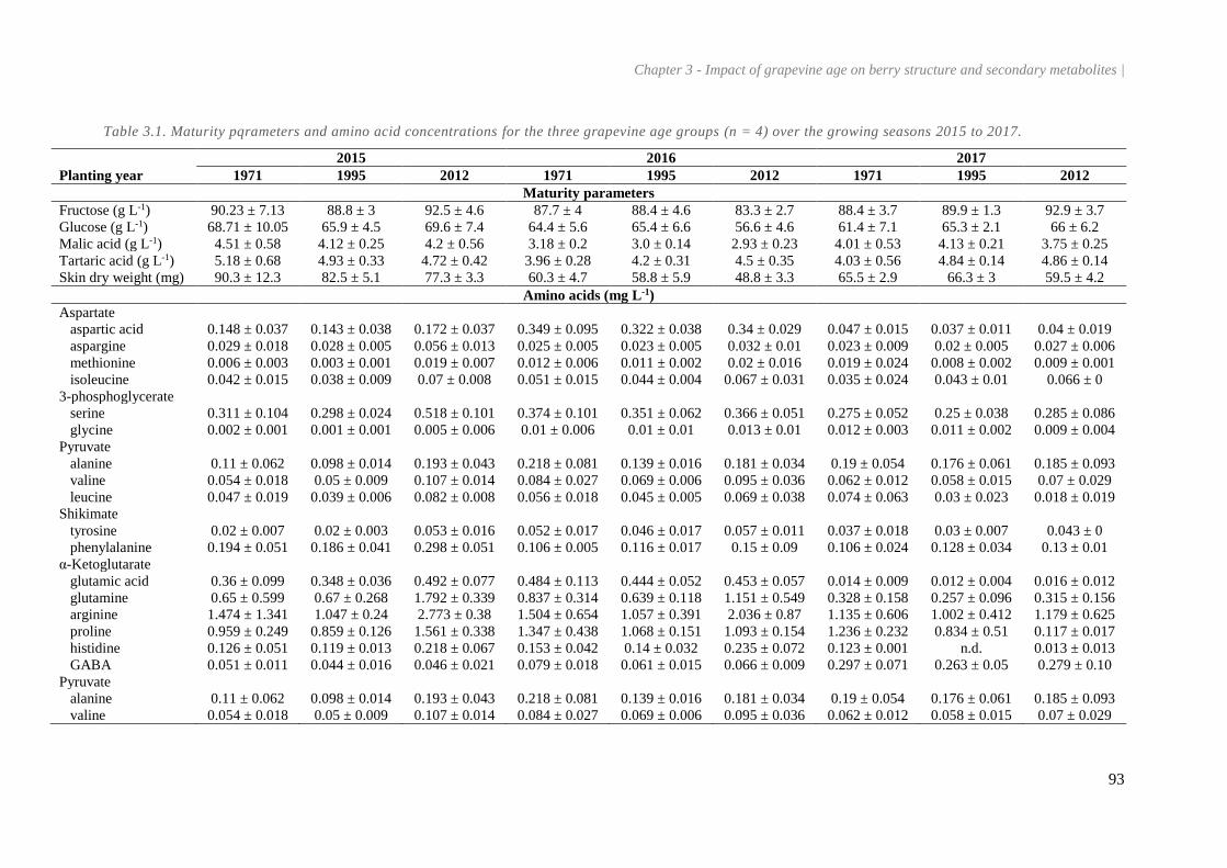
Chapter 3 - Impact of grapevine age on berry structure and secondary metabolites |
93
Table 3.1. Maturity pqrameters and amino acid concentrations for the three grapevine age groups (n = 4) over the growing seasons 2015 to 2017.
2015 2016 2017
Planting year 1971 1995 2012 1971 1995 2012 1971 1995 2012
Maturity parameters
Fructose (g L-1) 90.23 ± 7.13 88.8 ± 3 92.5 ± 4.6 87.7 ± 4 88.4 ± 4.6 83.3 ± 2.7 88.4 ± 3.7 89.9 ± 1.3 92.9 ± 3.7
Glucose (g L-1) 68.71 ± 10.05 65.9 ± 4.5 69.6 ± 7.4 64.4 ± 5.6 65.4 ± 6.6 56.6 ± 4.6 61.4 ± 7.1 65.3 ± 2.1 66 ± 6.2
Malic acid (g L-1) 4.51 ± 0.58 4.12 ± 0.25 4.2 ± 0.56 3.18 ± 0.2 3.0 ± 0.14 2.93 ± 0.23 4.01 ± 0.53 4.13 ± 0.21 3.75 ± 0.25
Tartaric acid (g L-1) 5.18 ± 0.68 4.93 ± 0.33 4.72 ± 0.42 3.96 ± 0.28 4.2 ± 0.31 4.5 ± 0.35 4.03 ± 0.56 4.84 ± 0.14 4.86 ± 0.14
Skin dry weight (mg) 90.3 ± 12.3 82.5 ± 5.1 77.3 ± 3.3 60.3 ± 4.7 58.8 ± 5.9 48.8 ± 3.3 65.5 ± 2.9 66.3 ± 3 59.5 ± 4.2
Amino acids (mg L-1)
Aspartate
aspartic acid 0.148 ± 0.037 0.143 ± 0.038 0.172 ± 0.037 0.349 ± 0.095 0.322 ± 0.038 0.34 ± 0.029 0.047 ± 0.015 0.037 ± 0.011 0.04 ± 0.019
aspargine 0.029 ± 0.018 0.028 ± 0.005 0.056 ± 0.013 0.025 ± 0.005 0.023 ± 0.005 0.032 ± 0.01 0.023 ± 0.009 0.02 ± 0.005 0.027 ± 0.006
methionine 0.006 ± 0.003 0.003 ± 0.001 0.019 ± 0.007 0.012 ± 0.006 0.011 ± 0.002 0.02 ± 0.016 0.019 ± 0.024 0.008 ± 0.002 0.009 ± 0.001
isoleucine 0.042 ± 0.015 0.038 ± 0.009 0.07 ± 0.008 0.051 ± 0.015 0.044 ± 0.004 0.067 ± 0.031 0.035 ± 0.024 0.043 ± 0.01 0.066 ± 0
3-phosphoglycerate
serine 0.311 ± 0.104 0.298 ± 0.024 0.518 ± 0.101 0.374 ± 0.101 0.351 ± 0.062 0.366 ± 0.051 0.275 ± 0.052 0.25 ± 0.038 0.285 ± 0.086
glycine 0.002 ± 0.001 0.001 ± 0.001 0.005 ± 0.006 0.01 ± 0.006 0.01 ± 0.01 0.013 ± 0.01 0.012 ± 0.003 0.011 ± 0.002 0.009 ± 0.004
Pyruvate
alanine 0.11 ± 0.062 0.098 ± 0.014 0.193 ± 0.043 0.218 ± 0.081 0.139 ± 0.016 0.181 ± 0.034 0.19 ± 0.054 0.176 ± 0.061 0.185 ± 0.093
valine 0.054 ± 0.018 0.05 ± 0.009 0.107 ± 0.014 0.084 ± 0.027 0.069 ± 0.006 0.095 ± 0.036 0.062 ± 0.012 0.058 ± 0.015 0.07 ± 0.029
leucine 0.047 ± 0.019 0.039 ± 0.006 0.082 ± 0.008 0.056 ± 0.018 0.045 ± 0.005 0.069 ± 0.038 0.074 ± 0.063 0.03 ± 0.023 0.018 ± 0.019
Shikimate
tyrosine 0.02 ± 0.007 0.02 ± 0.003 0.053 ± 0.016 0.052 ± 0.017 0.046 ± 0.017 0.057 ± 0.011 0.037 ± 0.018 0.03 ± 0.007 0.043 ± 0
phenylalanine 0.194 ± 0.051 0.186 ± 0.041 0.298 ± 0.051 0.106 ± 0.005 0.116 ± 0.017 0.15 ± 0.09 0.106 ± 0.024 0.128 ± 0.034 0.13 ± 0.01
α-Ketoglutarate
glutamic acid 0.36 ± 0.099 0.348 ± 0.036 0.492 ± 0.077 0.484 ± 0.113 0.444 ± 0.052 0.453 ± 0.057 0.014 ± 0.009 0.012 ± 0.004 0.016 ± 0.012
glutamine 0.65 ± 0.599 0.67 ± 0.268 1.792 ± 0.339 0.837 ± 0.314 0.639 ± 0.118 1.151 ± 0.549 0.328 ± 0.158 0.257 ± 0.096 0.315 ± 0.156
arginine 1.474 ± 1.341 1.047 ± 0.24 2.773 ± 0.38 1.504 ± 0.654 1.057 ± 0.391 2.036 ± 0.87 1.135 ± 0.606 1.002 ± 0.412 1.179 ± 0.625
proline 0.959 ± 0.249 0.859 ± 0.126 1.561 ± 0.338 1.347 ± 0.438 1.068 ± 0.151 1.093 ± 0.154 1.236 ± 0.232 0.834 ± 0.51 0.117 ± 0.017
histidine 0.126 ± 0.051 0.119 ± 0.013 0.218 ± 0.067 0.153 ± 0.042 0.14 ± 0.032 0.235 ± 0.072 0.123 ± 0.001 n.d. 0.013 ± 0.013
GABA 0.051 ± 0.011 0.044 ± 0.016 0.046 ± 0.021 0.079 ± 0.018 0.061 ± 0.015 0.066 ± 0.009 0.297 ± 0.071 0.263 ± 0.05 0.279 ± 0.10
Pyruvate
alanine 0.11 ± 0.062 0.098 ± 0.014 0.193 ± 0.043 0.218 ± 0.081 0.139 ± 0.016 0.181 ± 0.034 0.19 ± 0.054 0.176 ± 0.061 0.185 ± 0.093
valine 0.054 ± 0.018 0.05 ± 0.009 0.107 ± 0.014 0.084 ± 0.027 0.069 ± 0.006 0.095 ± 0.036 0.062 ± 0.012 0.058 ± 0.015 0.07 ± 0.029
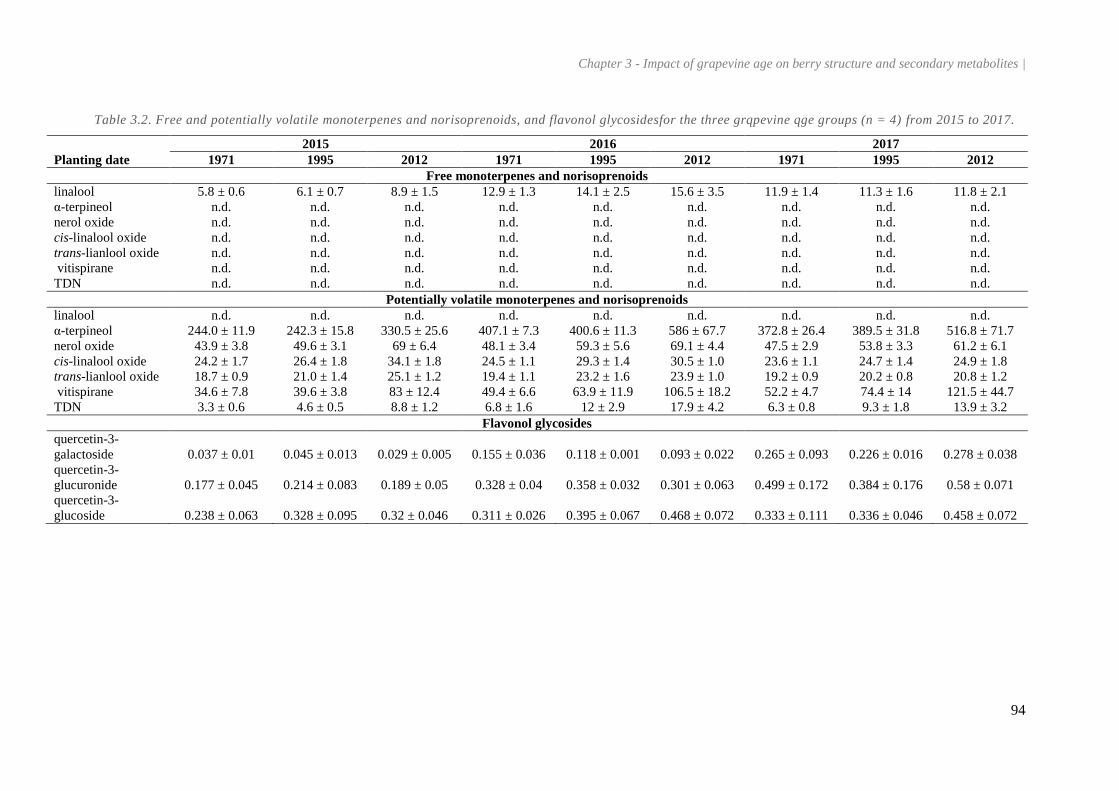
Chapter 3 - Impact of grapevine age on berry structure and secondary metabolites |
94
Table 3.2. Free and potentially volatile monoterpenes and norisoprenoids, and flavonol glycosidesfor the three grqpevine qge groups (n = 4) from 2015 to 2017.
2015 2016 2017
Planting date 1971 1995 2012 1971 1995 2012 1971 1995 2012
Free monoterpenes and norisoprenoids
linalool 5.8 ± 0.6 6.1 ± 0.7 8.9 ± 1.5 12.9 ± 1.3 14.1 ± 2.5 15.6 ± 3.5 11.9 ± 1.4 11.3 ± 1.6 11.8 ± 2.1
α-terpineol n.d. n.d. n.d. n.d. n.d. n.d. n.d. n.d. n.d.
nerol oxide n.d. n.d. n.d. n.d. n.d. n.d. n.d. n.d. n.d.
cis-linalool oxide n.d. n.d. n.d. n.d. n.d. n.d. n.d. n.d. n.d.
trans-lianlool oxide n.d. n.d. n.d. n.d. n.d. n.d. n.d. n.d. n.d.
vitispirane n.d. n.d. n.d. n.d. n.d. n.d. n.d. n.d. n.d.
TDN n.d. n.d. n.d. n.d. n.d. n.d. n.d. n.d. n.d.
Potentially volatile monoterpenes and norisoprenoids
linalool n.d. n.d. n.d. n.d. n.d. n.d. n.d. n.d. n.d.
α-terpineol 244.0 ± 11.9 242.3 ± 15.8 330.5 ± 25.6 407.1 ± 7.3 400.6 ± 11.3 586 ± 67.7 372.8 ± 26.4 389.5 ± 31.8 516.8 ± 71.7
nerol oxide 43.9 ± 3.8 49.6 ± 3.1 69 ± 6.4 48.1 ± 3.4 59.3 ± 5.6 69.1 ± 4.4 47.5 ± 2.9 53.8 ± 3.3 61.2 ± 6.1
cis-linalool oxide 24.2 ± 1.7 26.4 ± 1.8 34.1 ± 1.8 24.5 ± 1.1 29.3 ± 1.4 30.5 ± 1.0 23.6 ± 1.1 24.7 ± 1.4 24.9 ± 1.8
trans-lianlool oxide 18.7 ± 0.9 21.0 ± 1.4 25.1 ± 1.2 19.4 ± 1.1 23.2 ± 1.6 23.9 ± 1.0 19.2 ± 0.9 20.2 ± 0.8 20.8 ± 1.2
vitispirane 34.6 ± 7.8 39.6 ± 3.8 83 ± 12.4 49.4 ± 6.6 63.9 ± 11.9 106.5 ± 18.2 52.2 ± 4.7 74.4 ± 14 121.5 ± 44.7
TDN 3.3 ± 0.6 4.6 ± 0.5 8.8 ± 1.2 6.8 ± 1.6 12 ± 2.9 17.9 ± 4.2 6.3 ± 0.8 9.3 ± 1.8 13.9 ± 3.2
Flavonol glycosides
quercetin-3-
galactoside 0.037 ± 0.01 0.045 ± 0.013 0.029 ± 0.005 0.155 ± 0.036 0.118 ± 0.001 0.093 ± 0.022 0.265 ± 0.093 0.226 ± 0.016 0.278 ± 0.038
quercetin-3-
glucuronide 0.177 ± 0.045 0.214 ± 0.083 0.189 ± 0.05 0.328 ± 0.04 0.358 ± 0.032 0.301 ± 0.063 0.499 ± 0.172 0.384 ± 0.176 0.58 ± 0.071
quercetin-3-
glucoside 0.238 ± 0.063 0.328 ± 0.095 0.32 ± 0.046 0.311 ± 0.026 0.395 ± 0.067 0.468 ± 0.072 0.333 ± 0.111 0.336 ± 0.046 0.458 ± 0.072

Chapter 3 - Impact of grapevine age on berry structure and secondary metabolites |
95
Figure 3.1. PCA score plot of technological parameters and secondary metabolites (amino acids, quercetin
glucosides, and free and potentially volatile terpenes and norisoprenoids) from 2015-2017. The point
labels represent the growing season followed by the grapevine age group (‘O’ for ‘old’ grapevines planted
in 1971; ‘M’ for ‘mature’ grapevines planted in 1995; ‘Y’ for ‘young’ grapevines planted in 2012). There
are four replicates per growing season per age group, represented by the numbers 1 to 4 next to the letter.
Figure 3.2. Loadings plot of technological parameters and secondary metabolites (amino acids, quercetin
glucosides, and free and potentially volatile terpenes and norisoprenoids) from 2015-2017.
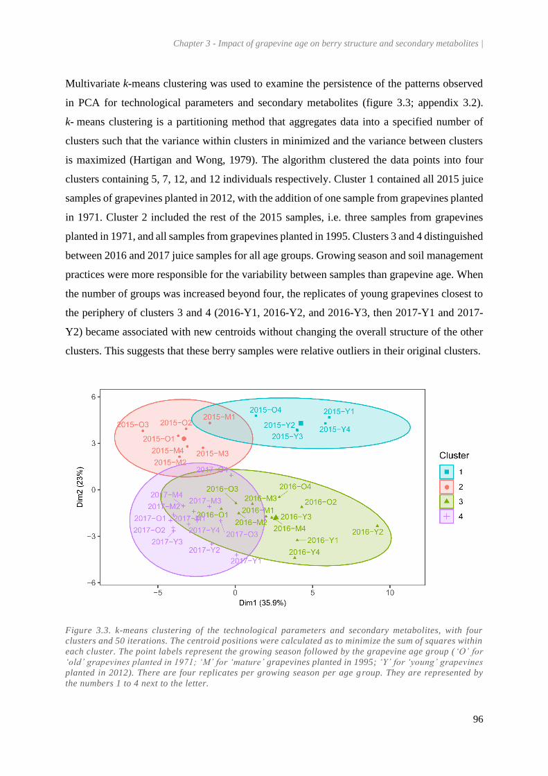
Chapter 3 - Impact of grapevine age on berry structure and secondary metabolites |
96
Multivariate k-means clustering was used to examine the persistence of the patterns observed
in PCA for technological parameters and secondary metabolites (figure 3.3; appendix 3.2).
k- means clustering is a partitioning method that aggregates data into a specified number of
clusters such that the variance within clusters in minimized and the variance between clusters
is maximized (Hartigan and Wong, 1979). The algorithm clustered the data points into four
clusters containing 5, 7, 12, and 12 individuals respectively. Cluster 1 contained all 2015 juice
samples of grapevines planted in 2012, with the addition of one sample from grapevines planted
in 1971. Cluster 2 included the rest of the 2015 samples, i.e. three samples from grapevines
planted in 1971, and all samples from grapevines planted in 1995. Clusters 3 and 4 distinguished
between 2016 and 2017 juice samples for all age groups. Growing season and soil management
practices were more responsible for the variability between samples than grapevine age. When
the number of groups was increased beyond four, the replicates of young grapevines closest to
the periphery of clusters 3 and 4 (2016-Y1, 2016-Y2, and 2016-Y3, then 2017-Y1 and 2017-
Y2) became associated with new centroids without changing the overall structure of the other
clusters. This suggests that these berry samples were relative outliers in their original clusters.
Figure 3.3. k-means clustering of the technological parameters and secondary metabolites, with four
clusters and 50 iterations. The centroid positions were calculated as to minimize the sum of squares within
each cluster. The point labels represent the growing season followed by the grapevine age group (‘O’ for
‘old’ grapevines planted in 1971; ‘M’ for ‘mature’ grapevines planted in 1995; ‘Y’ for ‘young’ grapevines
planted in 2012). There are four replicates per growing season per age g roup. They are represented by
the numbers 1 to 4 next to the letter.

Chapter 3 - Impact of grapevine age on berry structure and secondary metabolites |
97
3.2. Secondary metabolites and light interception
In 2014 and 2015, the youngest grapevines had thinner canopies and did not have a sufficient
bud fruitfulness to fill their allocated space on the trellis. Bunch exposure to light positively
impacts the concentration of monoterpenes, norisoprenoid and flavonols (Friedel et al., 2016;
Skinkis et al., 2010; Matus et al., 2009). PCA was thus undertaken with a focus on light-
sensitive compounds (monoterpenes, norisoprenoids, and flavonols) to assess the effect of
canopy microclimate identified earlier between grapevines planted in 2012 and grapevines
planted in 1995 and 1971 (Bou Nader et al., 2019).
Grapevines planted in 2012 were relatively more concentrated in monoterpenes, norisoprenoids,
and flavonols for all growing seasons (figure 3.4; appendix 3.3), although the specific
compounds varied from one season to the other. The first and second PCs were responsible for
82% of the variability in the data. The potentially volatile fractions of TDN, vitispirane and α-
terpineol were mostly correlated with PC 1, while PC 2 was mostly affected by quercetin-3-
galactoside and quercetin-3-glucuronide concentrations. Potential monoterpenes and
norisoprenoids were the most discriminant variables among samples. In 2017, only two berry
samples from vines planted in 2012 were still markedly different from other age groups, which
suggests that even though their characteristics were becoming similar to other age groups
specifically in amino acid content, there are still some differences with regards to their phenolic
and aroma composition.

Chapter 3 - Impact of grapevine age on berry structure and secondary metabolites |
98
Figure 3.4. PCA biplot of bound and free terpenes and quercetin glucosides in berry must at harvest from
2015 to 2017. The point labels represent the growing season followed by the grapevine age group ( ‘O’ for
‘old’ grapevines planted in 1971; ‘M’ for ‘mature’ grapevines planted in 1995; ‘Y’ for ‘young’ grapevines
planted in 2012). There are four replicates per growing season per age group. They are represented by
the numbers 1 to 4 next to the letter.
4. Conclusion
This work has focused on the canopy and cluster architecture of Riesling grapevines planted in
1971, 1995, and 2012 in the same vineyard from 2014 to 2017. It also assessed their berry
composition with regards to primary metabolites, amino acids, and aroma and phenolic
compounds.
Due to their young age, grapevines planted in 2012 were not subjected to the same soil treatment
as older groups in 2014 and 2015 and experienced a weak water deficit at the end of 2015 and
2016. They also had a thinner canopy at the beginning of the study. These factors, which are
difficult to clearly separate, had a large impact on the berry composition of the youngest
grapevines in their first vintages, with higher concentrations of amino acids but also higher free
and potentially volatile monoterpene and norisoprenoid content, and higher amounts of skin
flavonols. Grapevines planted in 1995 and 1971 had similar canopy and cluster architectures,

Chapter 3 - Impact of grapevine age on berry structure and secondary metabolites |
99
as well as comparable berry compositions throughout the study. This work suggests that the
impact of grapevine age is more important for young vines than fully established ones, mainly
for reasons related to different bud fruitfulness and vineyard management in early years, and
that these differences tend to disappear over a few years. More importantly, it was shown that
grapevines that were 19 and 43 years old did not have different berry compositions for the
studied compounds over a period of three to four years.

Chapter 4. Impact of grapevine age
on wine composition and sensory
attributes
This chapter is in preparation for publication in a modified version as:
Bou Nader, Khalil, Eric Gomès, Ghislaine Hilbert, Christel Renaud, Jean-Philippe Roby, Serge
Delrot, Hans R. Schultz, et al. “A Bottle of Old Vines Part 2. The Impact of Vine Age on
Riesling Wine Quality.” American Journal of Enology and Viticulture.
Author contributions: the author designed and conducted the sensory experiment, analyzed the data,
drafted and constructed the manuscript. Free and potential monoterpene and norisoprenoid
analysis, organic acid analysis, volatile sulfur compound analysis were performed by Stefanie
Fritsch, Heike Semmler, and Beata Beisert (Department of Microbiology and Biochemistry,
HGU). 1H NMR analysis was performed by Petra Kürbel (Department of Wine Analysis and
Beverage Technology, HGU). Sensory analysis was performed with Doris Häge (Department
of Enology, HGU).

Chapter 4 - Impact of grapevine age on wine composition and sensory attributes |
101
1. Introduction
Grapevine age and its relationship to wine quality has been a recurring topic of interest. Old
grapevines are usually held in high regard and are considered in many parts of the world as
belonging to cultural heritage (Barossa Chapters, 2018; Historic Vineyard Society, 2018). Some
winemaking regions even hold a register to track the age of vineyards and attribute a special
denomination to their wines, which are highly regarded and have a high reputation. It is
generally accepted that old grapevines have an improved balance between plant growth and
yield formation, which would hypothetically lead to richer, more concentrated berries and,
therefore, to an enhanced wine profile.
In the last decades, a few studies have attempted to confirm the supposed link between
grapevine age and wine quality, but research on the subject is still scarce. In one of the earliest
experiments to investigate wines from young and old vines, Heymann and Noble (1987)
performed descriptive sensory analysis on commercial Cabernet Sauvignon wines from several
regions in California, USA. The wines were produced from grapevines aged 5 to 20 years old.
A positive correlation was reported between grapevine age and berry aroma, while wines from
young grapevines were correlated with green bean and vegetal aromas with intensities that
depended on the region.
Reynold et al. (2008) studied Cabernet Sauvignon, Cabernet Franc, Pinot Noir, and Riesling
grapevines aged 4 and 14 years old over two growing seasons in Ontario, Canada. They reported
a higher concentration in phenolic compounds and anthocyanins for young grapevines. Sensory
analysis results for wines made from berries from grapevines of different age differed by
cultivar and growing season. Pinot Noir and Pinot Meunier wines from young grapevines were
rated higher for chocolate aroma, while Cabernet Sauvignon and Cabernet Franc wines from
young grapevines were lower in vegetal aroma in the first season.
In the same year in Wädenswil, Switzerland, Zufferey and Maigre (2008) compared wines from
three white cultivars (Chasselas, Arvine, and Pinot Blanc) and three red cultivars (Gamay,
Syrah, and Humagne Rouge) with respect to grapevine age. The sensory analysis of the vintages
2002 to 2006 showed that wines produced from old Gamay, Syrah and Humagne Rouge
grapevines were rated slightly better and described as having an improved tannic structure.
Conversely for white cultivars, there were no significant differences among grapevine ages for
Chapter 4 - Impact of grapevine age on wine composition and sensory attributes |
102
Chasselas and Arvine wines, and only wines of old Pinot Blanc grapevines were considered
better than those made from young grapevines (Zufferey and Maigre 2008).
The current study aims to add to the body of work on grapevine age and wine quality by
examining wines made from Vitis vinifera cv. Riesling grapevines of identical plant material,
but planted in 1971, 1995, and 2012 in a single vineyard. A descriptive sensory analysis of
wines from the 2014, 2015, and 2016 vintages was made in 2017. In parallel, the wines were
analyzed chemically with a focus on potential monoterpenes and norisoprenoids, volatile sulfur
compounds (VSC), organic acids, and higher alcohols. The project has also accumulated wines
from vintages as old as 2002. While these wines could not be submitted to sensory analysis due
to the low number of bottles remaining, they were analyzed in the same way as wines from
2014 to 2016.
2. Materials and methods
2.1. Experimental design and plant material
The study was performed in an experimental vineyard in Geisenheim, Germany, with
alternating rows of Vitis vinifera (L.) cv. Riesling grapevines (clone Gm 239-17) on 5C Teleki
rootstocks and trained in double Guyot. The vineyard was initially planted in 1971, but some
rows were uprooted in 1995 and 2012 replanted with the same plant material in order to obtain
four blocks with each grapevine age group. The plot is described in more detail in Bou Nader
et al. (2019). It was studied from 2014, which was the first year of harvest for grapevines planted
in 2012, until 2017.
A cover crop of grass and clover was sown in alternating rows, but the rows of grapevines
planted in 2012 were rows were ploughed in 2014 and 2015 to prevent excessive competition
during the early developmental stages of the grapevines (Williams et al., 1990). Afterwards,
these rows were sown with the same cover crop combination that already existed in 1995 and
1971 rows. Soil nitrate and water content from depths of 0 to 30 cm and from 30 to 60 cm were
significantly higher in 2014 and 2015 for rows planted in 2012, but after this period the three
age groups had similar soil nitrate and water contents (Bou Nader at al., 2019).
Grapevines planted in 2012 did not fill their allocated space on the trellis until 2016 due to their
lower bud fruitfulness in previous years (Bou Nader et al., in preparation, see chapter 3). This
increased light interception in the cluster zone.

Chapter 4 - Impact of grapevine age on wine composition and sensory attributes |
103
2.2. Winemaking
The project has accumulated wines since the 2002 vintage so the same winemaking procedure
was used for wines from 2014 to 2017. A total of 200 kg of healthy grapes were harvested for
each grapevine age group. The clusters were pressed without destemming and 45 mg L-1 of SO2
in the form of K2S2O5 was added. After settling for 18 h at around 16 °C, the three must samples
were racked from the lees and were transferred to one 50 L and one 25 L stainless steel tank.
All batches were inoculated with dry yeast (Saccharomyces cerevisiae, 10g dry wt/hL) and
were kept at 18 °C until the end of fermentation. After fermentation the 50 L container was
topped up by combing it with the 25 L volume, sulfur dioxide was adjusted to 40 mg L-1 free
SO2. After six months, wines were sterile filtered, bottled in 0.75 L bottles sealed with screw
caps and stored at 16°C until further analysis or sensory assessment.
2.3. Sensory analysis
Sensory evaluation was carried out in a laboratory equipped according to the ISO standard
8589:2007. The wine descriptive analysis (DA), which was conducted in July 2017 and was
limited to wines from 2014 to 2016 (nine wines total) because of the relatively low volume of
wine from previous vintages. Twelve trained panelists from the staff of Hochschule Geisenheim
University (eight women and four men, ranging from 22 to 63 years) were recruited for the
sensory assessment. All panelists underwent basic sensory training according to DIN EN ISO
8586:2014-05 and were familiar with Riesling wines and DA. The first few sessions were
dedicated to the generation of descriptive attributes with a subset of wines from the study. The
final attribute list contained one visual attribute (color intensity), nine aroma attributes (table
4.1), and three taste attributes (table 4.2). The color intensity standard consisted of a scale made
with five wine glasses. The first glass contained water and the four others contained an old
Riesling wine (Villa Monrepos Classic 2009, Hochschule Geisenheim University) with
concentrations 100% (not diluted), 75%, 50%, and 25%. One extra aroma attribute was added
to describe the general impression of the wine. Once the attributes were generated, the panelists
underwent odor recognition and scale training. Most aroma references were prepared by
soaking the product of interest in propanediol overnight then spiking a neutral Riesling wine
with the obtained solution on the day of the tasting. This procedure allowed to precisely vary
the intensity of aromas and to create standards that conformed to panelists’ perception of the
aromas in the wines.
Chapter 4 - Impact of grapevine age on wine composition and sensory attributes |
104
The panelists practiced blind odor and taste recognition over eight one-hour sessions. Fresh
references were prepared weekly and renewed whenever necessary. In the last three training
sessions, subsets from the studied wines were used to conduct practice evaluations after odor
and taste training. Samples were presented in a clear ISO 3591:1977 glass covered with a petri
dish for aroma conservation. Each glass contained around 30 mL of wine that was cooled to
13 °C. Panelists rated the samples on an unstructured line scale of from ‘0 = weak’ to ‘9 =
strong’. For general impression, the four descriptors (green, floral, fruity, and ripe) were printed
under the scale instead of ‘weak’ and ‘strong’. The attributes were presented to panelists in
groups according to modalities with color intensity first, followed by aroma attributes and taste
attributes. Panelists were given a 20 s break after rating each sample to cleanse their palate with
water and unsalted crackers (Matzo) if necessary. The data was collected on individual
computers using FIZZ Acquisition version 2.50 (Biosystèmes, Couternon, France). Consensus
results were shown to the panelists at the end of the training sessions with FIZZ Calculation
version 2.50 (Biosystèmes, Couternon, France) so that they could assess their performance
relative to the group.
The final DA evaluation session was performed in the same conditions as the training sessions.
The reference standards were given to the panelists before the session to refresh their memory
and remained accessible until the end of the tasting. The nine wine samples were presented in
three repetitions, served nomadically in randomized order with three-digit codes. The tasting
was done in triplicate (9 wines × 3 repetitions for every panelist). Each sample was followed
by a 20 s break, and each flight of nine wines was followed by a 5 min break.

Chapter 4 - Impact of grapevine age on wine composition and sensory attributes |
105
Table 4.1. Composition of aroma reference standards prepared using aroma standards by soaking in
propanediol (Pd).
Aroma references prepared by soaking in propanediol
Aroma attribute Reference in propanediol (Pd, 20% v/v) Reference volume added to 20
mL neutral wine
Citrus 0.5 g lemon zest in 20 mL Pd 2 mL
Peach 25 g peaches in syrup in 30 mL Pd 3 mL
Dry fruits 10 g dry apricots + 10 g dry prunes in 40 mL Pd 10 mL
Rose ½ white rose in 20 mL Pd 2 mL
Spicy 0.25 g black pepper + 0.75 g nutmeg in 20 mL Pd 0.5 mL
Vegetal 1 g grass in 20 mL Pd 1 mL + 1.5 mL canned white bean
brine†
Other aroma references
Aroma attribute Reference standard
Aging/kerosene 20 mL of old Riesling (Villa Monrepos Classic 2009, Hochschule Geisenheim
University).
Burnt rubber 0.2 g of burnt rubber band placed in a 10 mL vial.
Reductive The smell of fermented cabbage and/or rotten eggs. No reference standard produced.
General impression An abstract scale divided into four sections (green-floral-fruity-ripe).
†The canned white bean brine was added directly in the wine.
Table 4.2. Taste reference standards with low and high concentrations.
Taste attribute Low concentration High concentration
Sweetness 3.0 g L-1 fructose in water 7.0 g L-1 fructose in water
Sourness 0.6 g L-1 citric acid in water 1.0 g L-1 citric acid in water
Bitterness 0.1 g L-1 caffeine in water 0.3 g L-1 caffeine in water
2.4. Wine composition
2.4.1. Color measurement
Wine color was assessed by tristimulus colorimetry based on CIELab parameters lightness (L*),
red/green (a*) and yellow/blue (b*) (CIE, 1986). The spectra were registered directly on the
wine with a Unicam 500 UV/Vis spectrophotometer set to measure in the visible region
(λ = 380–770 nm) at constant intervals (Δλ = 2 nm) and integrated using the software
CromaLab®.

Chapter 4 - Impact of grapevine age on wine composition and sensory attributes |
106
2.4.2. Organic acids
Wine organic acids content were determined by HPLC according to Schneider et al. (1987). An
internal standard of formic acid was added to the wine samples (5 g L-1) and 5 μL of the mixture
were injected in a Agilent 1100 Series liquid chromatograph (Agilent Technologies, Santa Clara,
CA, USA) equipped with a variable wavelength detector. The separation was made with an
Allure Organic Acids column (Restek GmbH, Bad Homburg, Germany) with a 5 μm particle
size, 60 Å pore size, and dimensions of 250 mm × i.d. 4.6 mm, in conjunction with a security
guard cartridge C 18 of dimensions 4.0 × 3.0 mm (Phenomenex, Aschaffenburg, Germany).
The column was eluted with an aqueuous solution of sulfuric acid (0.0139% v/v) and ethanol
(0.5% v/v) at a flow rate of 0.6 mL/min and was operated at 46 °C. Compound detection was
performed at a wavelength of 210 nm.
2.4.3. Potentially volatile monoterpenes and C13-norisoprenoids
Potentially volatile monoterpenes and C13-norisoprenoids were analyzed by a modified solid-
phase extraction (SPE) for sample preparation (Günata et al. 1985) as described in Schüttler
(2012) and Schüttler et al. (2015), followed by gas chromatography coupled with mass
spectrometry (GC-MS). The method was adapted by replacing the enzymatic release of
aglycones by acid hydrolysis using the procedure described by Kosteridis et al. (1999).
Wine samples were maintained at 4 °C before analysis. Strata SDB-L cartridges containing 500
mg of styrene-divenylbenzene polymer (Phenomenex, Torrance, CA USA) were
preconditioned with 5 mL of pentane/dichloromethane (2/1 v/v), followed by 10 mL of
methanol, 10 mL of methanol/H2O (1/1 v/v) and 10 mL of H2O. Must samples of 50 mL were
diluted 1:1 with water and were spiked with octan-3-ol and 2.6-dimethylhept-5-en-2-ol (DMH)
as internal standards (c(octan-3-ol) = 50 µg L-1; c(DMH) = 25 µg L-1) and were loaded on the SPE
cartridges. It was washed again with 10 mL of water and dried for one hour with nitrogen under
vacuum (see above). After drying the samples were eluted with 10 mL of
pentane/dichloromethane (2/1 v/v). The eluates were dried with anhydrous sodium sulfate and
concentrated to a final volume of 50 µL under gentle nitrogen flow, and 2 µL were used to
analyze free monoterpenes and norisoprenoids by gas chromatography.
For bound monoterpenes and norisoprenoids the SPE cartridges were eluted with 10 mL of
ethyl acetate. The fractions were evaporated to dryness under vacuum with a rotary evaporator
(Büchi, Flawil, Switzerland) at water bath temperature 40 °C and p = 138 kPa. The residues
were resolved in 5 mL of 0.2 M citric acid (pH = 2.5), transferred to 10 mL head space vials,

Chapter 4 - Impact of grapevine age on wine composition and sensory attributes |
107
sealed, and heated in a laboratory oven at 100 °C for 60 min. After cooling down the samples
in ice, the internal standard mix was added based on the initial sample volume. Three successive
liquid-liquid extractions were conducted with 2 mL, 1 mL, and 1 mL pentane/dichloromethane
(2/1 v/v) and the recombined organic extracts were dried with anhydrous sodium sulfate and
concentrated under nitrogen flow to a final volume of 50 µL and 2 µL were injected for gas
chromatography. GC-MS was performed with a Thermo Fisher Trace GC Ultra gas
chromatograph equipped with a PTV injector and coupled to a Thermo Fisher ITQ 900 Ion Trap
MS mass spectrometric detector (Thermo Fisher Scientific, Waltham, MA USA). Two µL of
sample extract were injected in spitless mode (spitless time 90 s) at 200 °C. An Agilent DB-
Wax capillary column of dimensions 30 m × 0.25 mm ID × 0.5 µm film density (Agilent
Technologies, Santa Clara, CA USA) which was used for the separation. During injection, the
column oven was gradually heated to reach the following temperatures: 40 °C for 1 min, then
heated until 60 °C at 10 °C min-1, then from 60 °C to 200 °C at 3 °C min-1, and from 200 °C to
230 °C at 10 °C min-1. The temperature was finally maintained at 230 °C for 10 min. Helium
was used as a carrier gas with a flow of 1.4 mL min-1 and average velocity of 27 cm s-1. The
interface and MS source temperatures were set to 240 °C and 200 °C respectively. Mass
spectrometric data was acquired in electron impact mode (EI) with an ionization energy of 70
eV. The quantification of aroma compounds was made with the selected ion monitoring mode
(SIM).
2.4.4. Volatile sulfur compounds
Volatile sulfur compounds (VSC) were analyzed by gas chromatography coupled with a pulsed
flame photometric detector (PHPD) with headspace injection according to Rauhut et al. (2005)
and Schüttler et al. (2015). The equipment used for the analysis included a GC Hewlett Packard
(HP) 5890 Series II (Agilent, Waldbronn, Germany) equipped with cooled injection system
(CIS-3) (Gerstel GmbH, Mülheim an der Ruhr, Germany), a headspace single injection system
(HIS) (Gerstel GmbH, Mülheim an der Ruhr, Germany), and coupled to a PFPD Model 5380
(Ol Analytical, College Station, TX, USA). The liner was packed with 25 mg Porapak Q
80/100 mesh (Sigma-Aldrich, Seelze, Germany). The separation was made on a 30 m × 0.32
mm ID × 4 μm SBP-1 Sulfur column (Supelco, Bellefonte, PA, USA). The wine samples were
taken at 4 °C just before the sensory evaluation. Three mL of wine were pipetted into 5 mL GC
vials that were flused with argon and contained 4 mg L-1 2,6-di-tert-butyl-4-methyl-phenol,
0.27 g mL-1 NaCl, 0.2 g L-1 EDTA (ethylenediamine tetra acetic acid), and 500 mg L-1 propanal

Chapter 4 - Impact of grapevine age on wine composition and sensory attributes |
108
to bind SO2 molecules. An ethanolic internal standard of methyl-iso-propylsulfide and
butylmethylsulfide (8 μg L-1) was added before closing the vial with a magnetic screwcap. The
samples were preheated at 60 °C for 45 min before injection into the CIS-3. A total of 1000 μL
headspace volume were injected in solvent vent mode with helium gas (Linde Gas, Würzburg,
Germany). During injection the temperature was kept at 60 °C then increased to 180 °C with a
gradient of 12 °C/s and was held for 8 min. Oven temperature was kept at 35 °C for 5 min and
increased to 180 °C with a gradient of 10 °C/min and was kept for 10 min. The temperature of
the detector was maintained at 250 °C and air and hydrogen flows were maintained at a pressure
of 420 kPa.
2.4.5. NMR fingerprinting
The wines were analyzed by 1H NMR (nuclear magnetic resonance) for the quantification of
several compounds including alcohols and aldehydes (Godelmann et al., 2016, 2013). The
samples were diluted to 90% with a 1 M K2PO4 buffer (pH = 2.4) in D2O, with 3-
(trimethylsilyl)-propanoic acid sodium salt (TSP) as internal standard for referencing the
chemical shift to 0ppm. The pH of the mixture was adjusted to 3.10 ± 0.02 with 1 M NaOH or
HCl. A total of 600 μL were transferred to a 5 mm NMR tube and measured immediately.
Measurements were made with a 400 MHz Avance III NMR spectrometer (Bruker BioSpin
GmbH, Rheinstetten, Germany) equipped with a 5 mm 1H/D-TXI probehead with z-gradient,
automated tuning and matching accessory, and BTO-2000 for temperature control.
Measurements were made under water and ethanol suppression with the correction of eventual
interferences. Signal-to-noise (S/N) ratio was 10:1 and recycling time was 6 s. Temperature
was set to 300 ± 0.2 K without rotation. The pulse angle was maintained for the calibration and
measurement of wine samples and the sweep width (SW) was 18 ppm. Compound
quantification was performed by Bruker BioSpin GmbH according to Godelmann et al. (2016).
2.5. Statistical analysis
The statistical analysis was performed with RStudio (version 1.1.453; Rstudio, 2018) and R
(version 3.5.0; R Core Team, 2018). Analysis of variance (ANOVA) was used to assess the
panelists’ rating of the 2014, 2015, and 2016 wines. Principal component analysis (PCA) on
mean ratings was used to examine the relationships between the sensory attributes and the wines.
It was also used to assess the chemical composition of wines from older vintages. Multiple
factor analysis (MFA) was used to contrast the sensory and chemical descriptions of the tasted
wines. ANOVA analysis on wine sensory analysis was made with PanelCheck (Tomic et al.,

Chapter 4 - Impact of grapevine age on wine composition and sensory attributes |
109
2009). PCA and MFA were performed with the packages FactoMineR (version 1.41; Lê et al.,
2008) and factoextra (version 1.0.5; Kassambara and Mundt, 2017).
3. Results and discussion
3.1. Sensory analysis
The average ratings of the 14 attributes over the three tasting replicates are presented in table
4.3. All attributes except citrus (P = 0.20), rose (P = 0.51), and bitterness (P = 0.19) were
significantly different across wines (appendix 4.1). There were significant interactions for wine
× replicate for the attributes of color intensity (P = 0.046), peach (P = 0.033), and dry fruit (P
= 0.015). The interaction for color intensity may be due to the order of tasting, with wines that
are presented after a more intense wine being judged less intense than when following a light
wine. Peach and dry fruit attributes were the most difficult to differentiate for panelists despite
their training and experience.
PCA was used to examine the relationship between wines and attributes (figure 4.1). The first
two principal components (PCs) explained 82% of the variability in the data. The first PC
clustered several sensory attributes into a single group, with color intensity, peach, dry fruit,
spices, aging/kerosene, general impression, and sweetness being positively correlated. This
group was highly representative for the 2014 and 2015 wines from grapevines planted in 2012
(2014-Y and 2015-Y). The second PC was mostly affected by citrus, reductive, and burnt rubber
aromas. The latter two attributes described the 2014 and 2016 wines from grapevines planted
in 1995 (2014-M and 2016-M) and the 2016 wine from grapevines planted in 1971 (2016-O).
Eigenvalues and eigenvectors are presented in appendix 4.2.
The PCA separated wines by grapevine age but the differences were mostly present between
grapevines planted in 2012 and one hand and grapevines planted in 1995 and 1971 on the other.
Indeed, except for the 2014 vintage, wines from grapevines planted in 1995 and 1971 were
similar in sensory profile. Its results agree with the data obtained from berry composition (Bou
Nader et al., in preparation, chapter 3). During 2014 and 2015, grapevines planted in 2012 were
subjected to a different soil treatment (absence cover crop, ploughing) than older grapevine
groups due to their young age. This is likely to have increased soil nitrogen mineralization
(Davies et al., 2001), which in turn caused a higher nitrogen accumulation in the berries as
reported in raspberry (Zebarth et al., 2007). In the same period, young grapevines generally had
a lower bud fruitfulness than grapevines planted in 1995 and 1971. As a result, their clusters

Chapter 4 - Impact of grapevine age on wine composition and sensory attributes |
110
were better exposed to light in the cluster zone and a higher production of monoterpenes,
norisoprenoids, and skin flavonols (Bou Nader et al., in preparation, chapter 3). The berry
composition of grapevines planted in 2012 was similar to older groups once cover crop was
sown and they reached the same bud fruitfulness in 2016.

Chapter 4 - Impact of grapevine age on wine composition and sensory attributes |
111
Table 4.3. Average ratings per attribute in the 2017 tasting for wines from the three grapevine age groups (vintages 2014 to 2016). The means and standard
deviations were calculated from three replications with 12 panelists.
2014 2015 2016
Planting date 1971 1995 2012 1971 1995 2012 1971 1995 2012
color intensity 3.70 ± 1.28 3.06 ± 1.26 5.74 ± 1.33 4.02 ± 1.22 3.67 ± 1.27 6.29 ± 1.06 4.34 ± 1.25 3.47 ± 1.04 2.65 ± 0.92
citrus 2.32 ± 1.44 1.90 ± 1.39 1.93 ± 1.47 2.22 ± 1.24 2.36 ± 1.82 1.88 ± 1.37 2.15 ± 1.52 2.20 ± 1.07 2.52 ± 1.39
peach 2.28 ± 1.26 1.63 ± 1.38 2.40 ± 1.30 2.21 ± 1.49 1.89 ± 1.25 2.84 ± 1.78 1.43 ± 1.00 1.85 ± 1.52 1.87 ± 1.52
dry fruit 2.21 ± 1.62 1.10 ± 1.21 3.07 ± 1.72 2.40 ± 1.65 2.19 ± 1.54 4.35 ± 1.32 1.12 ± 1.31 0.93 ± 0.92 0.94 ± 0.93
rose 1.37 ± 0.87 1.19 ± 0.94 1.26 ± 0.98 1.40 ± 1.10 1.14 ± 1.13 1.27 ± 0.99 1.39 ± 1.17 1.49 ± 1.15 1.58 ± 1.30
vegetal 1.41 ± 1.58 1.57 ± 1.27 0.96 ± 1.21 1.17 ± 1.48 1.23 ± 1.39 0.59 ± 0.55 2.17 ± 1.47 2.07 ± 1.36 1.79 ± 1.30
spices 1.18 ± 1.06 0.71 ± 0.56 0.90 ± 0.62 1.11 ± 0.83 1.06 ± 0.81 1.25 ± 0.96 0.62 ± 0.41 0.58 ± 0.48 0.96 ± 0.93
aging/kerosene 2.42 ± 2.04 1.46 ± 1.85 3.94 ± 2.27 2.74 ± 1.8 2.83 ± 1.95 4.54 ± 2.34 1.20 ± 1.28 0.82 ± 0.75 0.84 ± 0.81
general impression 4.68 ± 2.50 2.86 ± 2.52 6.05 ± 1.92 4.77 ± 2.24 4.59 ± 2.59 7.23 ± 0.83 2.48 ± 1.88 2.38 ± 1.60 2.76 ± 1.77
reductive 0.64 ± 0.69 1.67 ± 1.85 0.60 ± 0.62 0.78 ± 1.0 0.70 ± 0.98 0.48 ± 0.56 1.28 ± 1.50 1.10 ± 1.22 1.04 ± 0.89
burnt rubber 1.14 ± 1.52 3.58 ± 2.60 0.94 ± 1.71 0.92 ± 1.27 1.04 ± 1.42 0.42 ± 0.42 3.86 ± 2.14 3.10 ± 1.98 2.77 ± 2.10
sourness 4.27 ± 1.86 4.50 ± 1.88 3.57 ± 1.68 5.38 ± 1.67 5.11 ± 1.91 3.31 ± 1.46 4.92 ± 1.66 5.05 ± 1.88 4.95 ± 1.72
sweetness 2.06 ± 1.45 1.71 ± 1.49 2.41 ± 1.40 1.77 ± 1.41 1.93 ± 1.56 4.45 ± 2.05 1.69 ± 1.19 1.57 ± 1.30 1.40 ± 1.15
bitterness 2.20 ± 1.85 2.24 ± 2.30 2.66 ± 2.25 2.68 ± 2.20 2.50 ± 1.93 1.79 ± 1.73 2.67 ± 2.30 2.46 ± 1.95 2.36 ± 2.01

Chapter 4 - Impact of grapevine age on wine composition and sensory attributes |
112
Figure 4.1. PCA biplot of the 2017 sensory analysis of grapevines from the three grapevine age groups.
The point labels represent the growing season followed by the grapevine age group ( ‘O’ for ‘old’
grapevines planted in 1971; ‘M’ for ‘mature’ grapevines planted in 1995; ‘Y’ for ‘young’ grapevines
planted in 2012). There are four replicates per growing season per age group, represented by the numbers
1 to 4 next to the letter.
3.2. Chemical analysis
The concentration of various compounds obtained from 1H NMR and HPLC, as well as free
and potential monoterpenes and norisoprenoids and VSCs are presented in appendices 4.3-4.6.
Among monoterpens and norisoprenoids, α-terpineol, hotrienol, cis- and trans-linalool oxides,
and TDN were found in free form in the wines, but only hotrienol and TDN had concentrations
around their odor thresholds (table 4.4). Hotrienol, with an odor threshold of 30 μg L-1 (Pino
and Fajardo, 2011) is characterized by a floral aroma. Its highest concentrations were reported
for wines from vintages 2012, 2014, and 2015. The norisoprenoid TDN, which has an odor
threshold of 2 to 20 μg L-1 (Ross et al., 2014; Sacks et al., 2012) and is responsible for the
typical kerosene like aroma of Riesling wines, was already present in free form at a
concentration of 1.8 μg L-1 for 2016 wines, and generally increased up to 14.6 μg L-1 for older
vintages. TDN is formed by the hydrolysis and rearrangement of carotenoid-derived precursors
during wine fermentation and storage (Sacks et al., 2012). Hence, potential TDN, which
represents the concentration of these precursors, was higher in younger wines, although the
concentration was dependent on the vintage.

Chapter 4 - Impact of grapevine age on wine composition and sensory attributes |
113
Hydrogen sulfide (H2S), dimethyl sulfide (DMS), and carbon disulfide (CS2) were the only
VSCs detected in the wine samples. These low-boiling point sulfur compounds do not occur in
grapes and are mostly generated during fermentation and storage from exogenous sulfate (SO42-)
and sulfite (SO32-) ions and subsequently from the sulfur-containing amino acids cysteine and
methionine (Smith et al., 2015). With the exception of H2S, these compounds can have a
positive effect on the complexity of wine aroma by interacting with other odorant molecules.
Specifically, DMS found at low concentrations can develop a blackcurrant or truffle aroma, but
is related to vegetal aromas like asparagus at high concentration (Segurel et al., 2004). The
wines of grapevines planted in 2012 had higher levels of H2S and DMS than wines from older
grapevines in 2014 and 2015, possibly due to the higher amino acid concentration in their juice
(Bou Nader et al., in preparation, chapter 3).
Table 4.4. List of the compounds analyzed in wine.
Free monoterpenes and norisoprenoids Volatile sulfur compounds Measured by 1H
NMR†
linalool hydrogen sulfide methanol
α-terpineol methanethiol 2,3-butanediol
hotrienol ethanethiol 2-phenylethanol
nerol oxide carbon disulfide 3-mehtylbutanol
cis-linalool oxide dimethyl sulfide glycerol
trans-lianlool oxide thioaceticacid -S- methyl ester acetaldehyde
vitispirane thioaceticacid -S- ethyl ester ethyl acetate
TDN dimethyl disulfide succinic acid
Potential monoterpenes and norisoprenoids diethyl disulfide galacturonic acid
linalool dimethyl trisulfide caftaric acid
α-terpineol Organic acids CIELab color space
hotrienol tartaric Acid L*
nerol oxide malic Acid a*
cis-linalool oxide shikimic Acid b*
trans-lianlool oxide lactic Acid
vitispirane acetic Acid
TDN citric Acid †Several classes of compounds.
3.3. MFA with chemical and sensory data
Multiple factor analysis (MFA) was used to relate the chemical data obtained for wine to the
sensory attributes. MFA is a relatively recent factorial method that can analyze datasets
consisting of several groups of variables defined on the same set of individuals. It allows the

Chapter 4 - Impact of grapevine age on wine composition and sensory attributes |
114
group matrices to be scaled individually before concatenating them and performing principal
component analysis (Escofier and Pagès, 1994).
The first and second PCAs accounted for 70% of the total variability between wine samples
(figure 4.2; appendix 4.7). The separation of sensory attributes that was visible in PCA was
conserved, with attributes related to ripeness grouped together on the right-hand side of the
MFA loadings plot. These attributes were positively correlated with the b* component of the
CIELab color space, which takes positive values for yellow. They were also positively
correlated with concentrations of free TDN, DMS, and H2S. The left-hand side of the MFA
loadings plot regrouped attributes linked to greenness such as citrus, vegetal, and rose, but also
the reductive and burnt rubber aromas. Sourness was also part of this group of variables and
was related to citrus aroma and the concentration of tartaric acid. Finally, the rose attribute,
even though it did not significantly vary across wines, was correlated with succinic acid,
methylbutanol, and phenylethanol, which havea light floral aroma (García et al., 2003; Maoz et
al., 2018). The second PCA was mostly defined by potential TDN and α-terpineol, as well as
lactic acid. In fact, most potentially volatile monoterpenes and norisoprenoids were located on
the bottom right of the loadings plot, while their free counterparts were clustered in the top right.
In 2014 and 2015 the wines from grapevines planted in 2012 were correlated with the group of
ripeness attributes and potential monoterpenes and norisoprenoids, while wines from
grapevines planted in 1995 and 1971 were grouped together (figure 4.3). In 2016 there was a
high agreement within the sensorial panel between the three wine samples with regard to
sensory and chemical profile. The trend seen in MFA mirrored the trend of berry composition,
where the berry composition of grapevines planted in 2012 converged with older grapevines
after cover crop was sown and they had reached their bud fruitfulness potential.

Chapter 4 - Impact of grapevine age on wine composition and sensory attributes |
115
Figure 4.2. MFA Loadings plot of the sensory and chemical and sensory variables analyzed in 2017.
Figure 4.3. MFA partial score plot with chemical sensory variables analyzed in 2017. The point labels
represent the growing season followed by the grapevine age group (‘O’ for ‘old’ grapevines planted in
1971; ‘M’ for ‘mature’ grapevines planted in 1995; ‘Y’ for ‘young’ grapevines planted in 2012). There
are four replicates per growing season per age group, represented by the numbers 1 to 4 next to the letter.
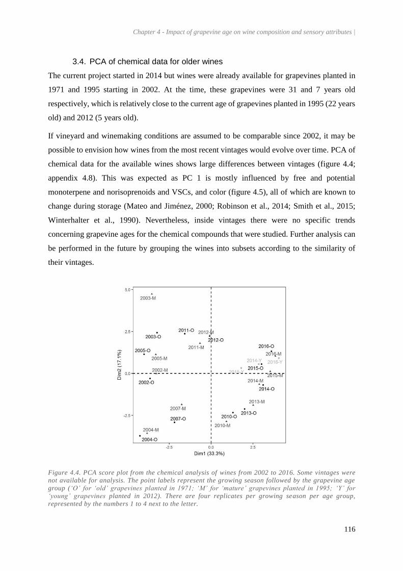
Chapter 4 - Impact of grapevine age on wine composition and sensory attributes |
116
3.4. PCA of chemical data for older wines
The current project started in 2014 but wines were already available for grapevines planted in
1971 and 1995 starting in 2002. At the time, these grapevines were 31 and 7 years old
respectively, which is relatively close to the current age of grapevines planted in 1995 (22 years
old) and 2012 (5 years old).
If vineyard and winemaking conditions are assumed to be comparable since 2002, it may be
possible to envision how wines from the most recent vintages would evolve over time. PCA of
chemical data for the available wines shows large differences between vintages (figure 4.4;
appendix 4.8). This was expected as PC 1 is mostly influenced by free and potential
monoterpene and norisoprenoids and VSCs, and color (figure 4.5), all of which are known to
change during storage (Mateo and Jiménez, 2000; Robinson et al., 2014; Smith et al., 2015;
Winterhalter et al., 1990). Nevertheless, inside vintages there were no specific trends
concerning grapevine ages for the chemical compounds that were studied. Further analysis can
be performed in the future by grouping the wines into subsets according to the similarity of
their vintages.
Figure 4.4. PCA score plot from the chemical analysis of wines from 2002 to 2016. Some vintages were
not available for analysis. The point labels represent the growing season followed by the grapevine age
group (‘O’ for ‘old’ grapevines planted in 1971; ‘M’ for ‘mature’ grapevines planted in 1995; ‘Y’ for
‘young’ grapevines planted in 2012). There are four replicates per growing season per age group,
represented by the numbers 1 to 4 next to the letter.

Chapter 4 - Impact of grapevine age on wine composition and sensory attributes |
117
Figure 4.5. PCA loadings plot from the chemical analysis of wines from 2002 to 2016.
4. Conclusion
The wines from Riesling grapevines planted in 1971, 1995, and 2012 were evaluated by sensory
descriptive analysis and chemical analysis. The largest variability in the samples, both in
sensory and chemical analysis, was found for wines from the first vintages of grapevines
planted in 2012 and was likely caused by differences in soil management and an inherently
lower bud fruitfulness. Wines produced from these grapevines were highly colored and were
associated with aromas of kerosene and ripe fruits and with free and potential monoterpenes
and norisoprenoids and VSC. In the third vintage, wines from grapevines planted in 2012 had
similar chemical and sensory profiles than wines from older age groups. Wines from older
vintages were also analyzed chemically. Vintage effects were more important than the variance
due to grapevine age.

Chapter 5. Evaluating grapevine
trunk size with a handheld camera
by 3D modeling
This chapter was submitted for publication in a modified version as:
Bou Nader, Khalil, Leonard Maximilian Pfahl, Eric Gomès, and Manfred Stoll. “Evaluating
Grapevine Trunk Size with a Handheld Camera by 3D Modeling.” OENO One.
Author contributions: the author designed the research experiment and drafted the manuscript. The
experiment, analysis of the data and construction of the manuscript were conducted with
Leonard Maximilian Pfahl. The modeling was performed by Leonard Maximilian Pfahl.

Chapter 5 - Evaluating grapevine trunk size with a handheld camera by 3D modeling |
119
1. Abstract
Background and aims: Grapevine size measurements are necessary to assess their carbon
reserves at single vine level and study the carbon sequestration potential of vineyards. These
measurements mostly rely on traditional dendrology techniques that may be prone to errors.
Here we examine the applicability of structure-from-motion with multi-view stereo-
photogrammetry (SfM-MVS) to accurately measure vine trunk thickness and volume. SfM-
MVS allows the creation of scaled, georeferenced 3D models based on a set of overlapping
photographs.
Methods and results: The study was conducted on field-grown Vtis vinifera L. cv. Riesling
vines aged 5, 22, and 46 years and pruned in a bilateral Guyot. Trunk diameter, cross-sectional
area and circumference 10 cm above the grafting point were measured with traditional
dendrometry and compared with values obtained from the reconstructed 3D models. SfM-MVS
was also used to estimate the total trunk volume and the contribution of the vine crown to this
volume. The correlations between measured and modeled metrics were close to unity (0.976 ≤
R2 ≤ 0.988). The estimates for 5-year-old vines had the largest errors due to their small trunk
size (RMSEdrow = 18.59%, RMSEdper = 14.19%, RMSETCSA = 20.97%, RMSEcircumference =
3.40%). In fact, the volume of 46-year-old vine trunks was 1.7 times greater than 22-year-old
vine trunks and more than 10 times greater than 5-year-old trunks. The vine crown contribution
to the total trunk volume was as high as 60% for the two older vine groups, and most of its size
increase occurred in the early stages of grapevine development.
Conclusions: SfM-MVS was able to produce accurate models of the vine trunks provided
adequate lighting conditions and image resolution.
Significance of the Study: This work serves as a proof of concept for the use of SfM-MVS to
measure the trunk size of field-grown grapevines of different ages. The technique, which is
relatively new, is cost-effective and easy to implement. Future research is necessary to
determine specific applications where it could assist or replace traditional dendrology methods.
Keywords: dendrology, vine age, carbon storage, wood reserves, photogrammetry, SfM-MVS.
2. Introduction
Trunk dimensions and structure (Tyminski, 2013) are often assessed in the fields of forestry,
ecology, and arboriculture. Their measurement at the single tree and forest scales allow the
evaluation of wood volume and biomass, water limitations, carbon stocks, as well as

Chapter 5 - Evaluating grapevine trunk size with a handheld camera by 3D modeling |
120
environmental and commercial values (Daudet et al., 2005; Houghton, 2005; Mlambo et al.,
2017; Nowak et al., 2013). Traditional dendrology methods have also been applied in viticulture
for determining grapevine age and annual growth rate (Tyminski, 2013). Knowledge about
grapevine carbon storage capacity and reallocation dynamics is essential to study the potential
of vineyards for carbon sequestration in permanent organs (trunk and roots) but also necessary
to assess the effect of management strategies on grapevine performance (Miranda et al., 2017;
Schreiner et al., 2006).
Grapevine perennial structure and production capacity increase with age, especially in the first
years after planting (Bou Nader et al., 2019; Chiarawipa et al., 2013; Grigg et al., 2017) but
their evolution depends on several environmental factors such as soil profile and depth, water
availability, and climate (Keller M., 2010). Grapevines present unique challenges compared to
tree species. Because of their liana nature, they can be trained into various systems to optimize
vigor and canopy light interception (Reynolds and Vanden Heuvel, 2009), adapt to
environmental and climatic factors (Palliotti et al., 2014), and reduce the incidence of fungal
infections (Austin et al., 2009). This results in a wide variety of grapevine trunk structures, thus
limiting the use of simple measurements such as trunk circumference when comparing multiple
training systems. In addition, traditional dendrology methods that produce the most accurate
results are often expensive, labor-intensive, and destructive, requiring plants to be uprooted for
measurement, while those that are simple and cost-effective are often prone to errors (Kitahara
et al., 2010).
Structure-from-motion with multi-view stereo-photogrammetry (SfM-MVS) is a recent
photogrammetric approach that automatically combines overlapping 2D images to create 3D
models of captured objects. It operates by identifying and matching object features across
images, then using these features to infer camera location and orientation (James and Robson,
2012). The technique has already been tested with success for the description of tree structures
(Liang et al., 2014; Miller et al., 2015; Morgenroth and Gomez, 2014).
The following paper is primarily intended as a proof of concept for the application of SfM-MVS in
viticulture by comparing the trunk circumference and cross-sectional area measured in the field on
grapevines of different ages to values derived from 3D model reconstruction. Secondly, it provides
a measure of the total volume of the trunk and also gives the opportunityto divide it into parts,
which might be of interest if parts of the trunk should not be taken into consideration, i.e. the
crown of the trunk in the case of older grapevines.

Chapter 5 - Evaluating grapevine trunk size with a handheld camera by 3D modeling |
121
3. Materials and methods
3.1. Plant material and field-measured trunk diameter and circumference
The trial was conducted in an experimental vineyard at the Hochschule Geisenheim University
(HGU) in Geisenheim, Germany (+49° 98’ 76.59”, +7° 94’ 47.90”). The vineyard was initially
planted in 1971 with Vitis vinifera (L.) cv. Riesling, clone Gm239-17, grafted on 5C Teleki
rootstock. Grapevines were distributed along 68 rows in a North-South orientation and cane-
pruned to form a bilateral, downward-arched Guyot. In 1995 and 2012, several rows were
uprooted and replanted with the same planting material. The end result was a vineyard with
identical grapevines of three different ages divided in alternating rows. The year 2014 was the
first productive vintage for grapevines planted in 2012. At that time, some grapevines were
already missing in the rows planted in 1971 and 1995. A fully randomized block experimental
design was therefore not possible to implement. Instead, a selection process was carried out at
the beginning of the 2014 growing season in order to select six grapevines per age group and
field replicate (n = 24). The number of nodes retained was adjusted to 10 per meter (equivalent
to 14 nodes per vine) during winter pruning. At the beginning of the growing season, the trunk
diameter in the direction of the row was measured 10 cm above the grafting point with an digital
caliper. This value, coupled with bud fruitfulness, was used to compare individual grapevines
to the row medians and means, and the three grapevines closest to these values were selected.
More weight was given to trunk diameter in the selection process because of its higher stability
across growing seasons. The selected grapevines were used in a separate trial on the impact of
grapevine age on productivity and water stress tolerance (Bou Nader et al., 2019). The current
trial was conducted in 2017, when the yield and pruning weight of grapevines planted in 2012
was similar to those of older grapevines (table 5.1).
Table 5.1. Overview of the three grapevine ages used in the 2017 study on trunk size.
Planting
year
Age
(years)
Variety/
Clone
Rootstock Pruning
system
Row ×
grapevine
distance (m)
Mean pruning
weight† (kg/m)
Mean yield†
(kg/m)
1971 5 Riesling/
Gm239-17
5C Teleki Bilateral
Guyot
2.0 × 1.4 0.78 ± 0.06 1.81 ± 0.20
1995 22 Riesling/
Gm239-17
5C Teleki Bilateral
Guyot
2.0 × 1.4 0.71 ± 0.09 2.23 ± 0.46
2012 46 Riesling/
Gm239-17
5C Teleki Bilateral
Guyot
2.0 × 1.4 0.67 ± 0.09 2.07 ± 0.33
†Values for the 2016 growing season.

Chapter 5 - Evaluating grapevine trunk size with a handheld camera by 3D modeling |
122
When the trunk diameter in the row direction was measured, a thin plastic cord was tied to the
trunk just under the caliper position to serve as a reference point for further measurements
(figures 5.1a and 5.1b). The diameter was measured again in the direction perpendicular to the
row. The two values were averaged and used to compute the trunk cross-sectional area (TCSA)
by approximating the trunk to a disc (Lepsis and Blanke, 2006). The trunk circumference was
measured with a flexible measuring tape at the same position.
3.2. Image acquisition for trunk reconstruction
The ground around the trunks was manually weeded to have a direct visual access to the trunk
base. Loose bark pieces were removed by gently whisking over the trunk to prevent volume
miscalculations. In order to georeference the images, a reference grid made of seven equally
spaced markers (Agisoft LLC, 2014) printed on cardboard was laid down on the ground around
the trunk before it was photographed (figure 5.1c). Models built with SfM-MVS initially do not
have any scale or georeference, and this information can be manually supplied to the software
with an object of known dimensions that is placed in the image (in this case the distance between
two adjacent markers, which was equal to 10.5 cm).
Figure 5.1. Example of the experimental setup for taking the pictures (a) with a general view of grapevine
with the georeference grid and the point of measurement (white arrow); (b) focus on the point of
measurement of trunk circumference and cross-sectional area 10 cm above the grafting point highlighted
in the field using a plastic cord; (c) focus on the georeference grid around the base of the trunk.
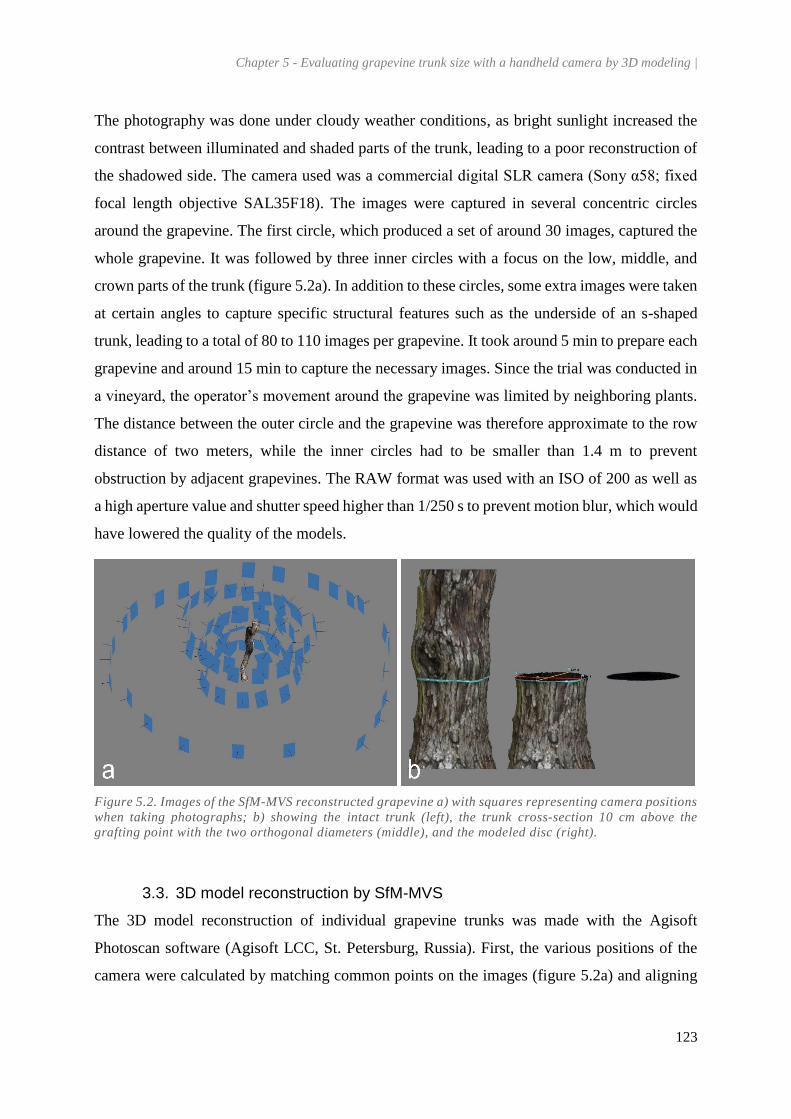
Chapter 5 - Evaluating grapevine trunk size with a handheld camera by 3D modeling |
123
The photography was done under cloudy weather conditions, as bright sunlight increased the
contrast between illuminated and shaded parts of the trunk, leading to a poor reconstruction of
the shadowed side. The camera used was a commercial digital SLR camera (Sony α58; fixed
focal length objective SAL35F18). The images were captured in several concentric circles
around the grapevine. The first circle, which produced a set of around 30 images, captured the
whole grapevine. It was followed by three inner circles with a focus on the low, middle, and
crown parts of the trunk (figure 5.2a). In addition to these circles, some extra images were taken
at certain angles to capture specific structural features such as the underside of an s-shaped
trunk, leading to a total of 80 to 110 images per grapevine. It took around 5 min to prepare each
grapevine and around 15 min to capture the necessary images. Since the trial was conducted in
a vineyard, the operator’s movement around the grapevine was limited by neighboring plants.
The distance between the outer circle and the grapevine was therefore approximate to the row
distance of two meters, while the inner circles had to be smaller than 1.4 m to prevent
obstruction by adjacent grapevines. The RAW format was used with an ISO of 200 as well as
a high aperture value and shutter speed higher than 1/250 s to prevent motion blur, which would
have lowered the quality of the models.
Figure 5.2. Images of the SfM-MVS reconstructed grapevine a) with squares representing camera positions
when taking photographs; b) showing the intact trunk (left), the trunk cross-section 10 cm above the
grafting point with the two orthogonal diameters (middle), and the modeled disc (right).
3.3. 3D model reconstruction by SfM-MVS
The 3D model reconstruction of individual grapevine trunks was made with the Agisoft
Photoscan software (Agisoft LCC, St. Petersburg, Russia). First, the various positions of the
camera were calculated by matching common points on the images (figure 5.2a) and aligning

Chapter 5 - Evaluating grapevine trunk size with a handheld camera by 3D modeling |
124
them to produce a sparse point model. Next, a dense point model in which points are several
times more numerous was generated. At this time the point cloud already resembles the original
grapevine but needs to be cleaned of noise coming from background elements, the ground,
trellis wires and posts, as well as false points that are sometimes caused by shadows. For the
purpose of this experiment, the trunk was truncated at the grafting point and the bilateral canes
were excluded. Finally, a polygonal mesh was fitted to the dense point model to form the 3D
trunk models.
As noted previously, the models do not yet have a scale or geographic position. To measure
distance or volume it is necessary to implement a coordinate system and a measuring scale.
After specifying the distance between markers on the georeferenced grid, the software can
create a coordinate system that allows data acquisition from various point. In some cases the
software failed to automatically identify all markers, so missing markers were manually
referenced.
3.4. SfM-MVS measurements and model validation
The trunk diameters in the direction of the row and perpendicular to the row were estimated on
the 3D models at the level of the plastic cord. The trunk was truncated at the measuring point,
and point markers were added based on the position of the georeferenced grid relative to the
trunk (figure 5.2b). For TCSA and trunk circumference it was necessary to create a surface at
the cross-section. This was done with the ‘close holes’ tool in Agisoft, which generates a
‘watertight’ mesh by connecting the points at the periphery of holes with a flat surface. It was
then possible to measure the trunk circumference TCSA directly on the surface without having
to rely on the orthogonal diameter (figure 5.2b). The values obtained for the metrics were
compared with field-measured values for validation.
3.5. Estimation of trunk volume and crown contribution
The computation of the total trunk volume also required the use of the ‘close holes’ tool.
However, the trunk volume that was calculated with the model could not be validated with field
measurements, as it would have been necessary to uproot the grapevines to obtain an accurate
volume of the trunk (Özçelik et al., 2008). This was not possible due to ongoing trials on the
72 selected grapevines.
It was apparent during measurements that the crowns of older grapevines formed more or less
important part of the total trunk volume. The grapevine crown is formed over the years after

Chapter 5 - Evaluating grapevine trunk size with a handheld camera by 3D modeling |
125
successive pruning, and depending on pruning techniques may contain dead wood. The
contribution of the grapevine crown to the total trunk volume was assessed by excluding it from
the model and comparing the volume obtained to the total volume. Since the grapevines were
approximately trained to the same height it was possible to estimate the minimal trunk height
before the crown. After visual inspection of all grapevine models, it was decided to keep 40 cm
of trunk above the grafting point for measurements and omit the fraction of the trunk above this
limit (figures 5.3a and 5.3b).
Figure 5.3. (a) Example of a complex crown on a 46 year old vine; (b) removal of the crown by truncating
the trunk volume to 40 cm above the grafting point.
3.6. Statistical analysis
The dendrological parameters derived from the 3D models were compared to the traditional
field measurements by linear regression with an estimation of R2. In addition to this procedure,
the root mean square error (RMSE) and bias as defined by equations 1 and 2 were calculated
for each grapevine age according to Kankare et al. (2013) and Miller et al. (2015):
𝑅𝑀𝑆𝐸 = √∑ (𝑦𝑖 − 𝑦𝑖)2𝑛𝑖=1
𝑛 Equation 1
𝐵𝑖𝑎𝑠 =∑ (𝑦𝑖 − 𝑦𝑖)𝑛𝑖=1
𝑛 Equation 2
where n is the number of estimates, yi is the value estimated by model reconstruction, and ŷi is
the value measured directly in the vineyard. Calculations were made with R (version 3.5.1; R
Core Team, 2018) and RStudio (version 1.1.419; RStudio, 2018).
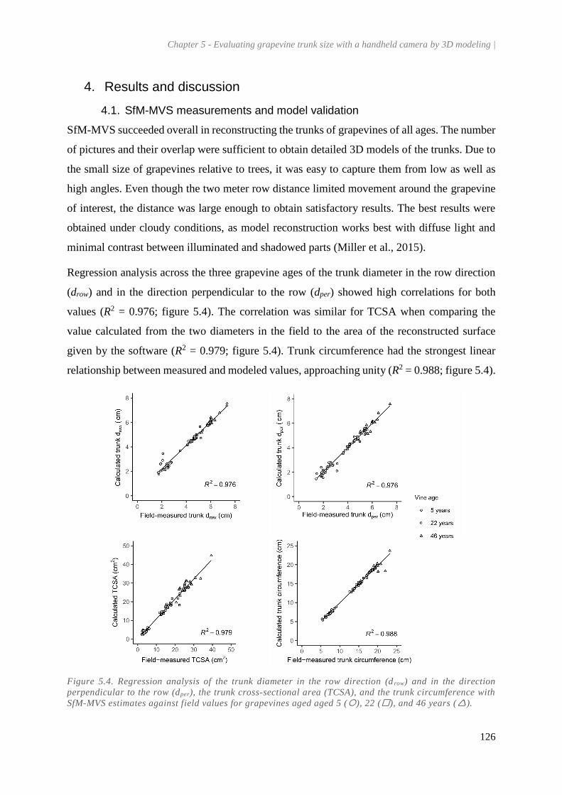
Chapter 5 - Evaluating grapevine trunk size with a handheld camera by 3D modeling |
126
4. Results and discussion
4.1. SfM-MVS measurements and model validation
SfM-MVS succeeded overall in reconstructing the trunks of grapevines of all ages. The number
of pictures and their overlap were sufficient to obtain detailed 3D models of the trunks. Due to
the small size of grapevines relative to trees, it was easy to capture them from low as well as
high angles. Even though the two meter row distance limited movement around the grapevine
of interest, the distance was large enough to obtain satisfactory results. The best results were
obtained under cloudy conditions, as model reconstruction works best with diffuse light and
minimal contrast between illuminated and shadowed parts (Miller et al., 2015).
Regression analysis across the three grapevine ages of the trunk diameter in the row direction
(drow) and in the direction perpendicular to the row (dper) showed high correlations for both
values (R2 = 0.976; figure 5.4). The correlation was similar for TCSA when comparing the
value calculated from the two diameters in the field to the area of the reconstructed surface
given by the software (R2 = 0.979; figure 5.4). Trunk circumference had the strongest linear
relationship between measured and modeled values, approaching unity (R2 = 0.988; figure 5.4).
Figure 5.4. Regression analysis of the trunk diameter in the row direction (d row) and in the direction
perpendicular to the row (dper), the trunk cross-sectional area (TCSA), and the trunk circumference with
SfM-MVS estimates against field values for grapevines aged aged 5 (), 22 (), and 46 years ().

Chapter 5 - Evaluating grapevine trunk size with a handheld camera by 3D modeling |
127
Although linear regression for the three grapevine ages combined showed a good fit of the data,
the RMSE and bias of the modelled data were generally higher for younger grapevines (table
5.2). This was especially true for 5-year-old grapevines, for which the impact of measurement
errors was magnified due to the small size of their trunk. The decrease in accuracy for 5-year-
old grapevines may also be related to the higher difficulty of applying SfM-MVS on small
objects such as slender tree branches (Kankare et al., 2013; Morgenroth and Gomez, 2014). The
density of point clouds generated by the software depends on image resolution, and it is
therefore affected by the camera and the distance at which the images are taken (James and
Robson, 2012).
Table 5.2. Field-measured and modeled metrics for 5-year-old, 22-year-old, and 46-year-old grapevines
(presented as mean ± sandard deviation) and the root mean square error (RMSE) and bias of modelled
data.
Metric Meanmeasured Meanmodeled RMSE† Bias† RMSE
(%)
Bias
(%)
5-year-old vines
drow (cm) 2.21 ± 0.29 2.40 ± 0.36 0.41 0.19 18.59 8.67
dper (cm) 2.21 ± 0.46 2.20 ± 0.40 0.31 0.00 14.19 -0.20
TCSA (cm2) 3.90 ± 1.10 4.16 ± 0.97 0.82 0.26 20.97 6.61
circumference (cm) 7.23 ± 0.96 7.18 ± 0.85 0.25 -0.04 3.40 -0.60
22-year-old vines
drow (cm) 4.59 ± 0.40 4.67 ± 0.40 0.19 0.07 4.22 1.61
dper (cm) 4.50 ± 0.52 4.50 ± 0.49 0.17 0.00 3.79 0.02
TCSA (cm2) 16.34 ± 3.80 17.45 ± 2.81 1.85 1.11 11.34 6.80
circumference (cm) 14.85 ± 2.44 14.76 ± 1.18 0.28 -0.09 1.90 -0.59
46-years-old vines
drow (cm) 5.97 ± 0.57 6.03 ± 0.62 0.14 0.07 2.42 1.12
dper (cm) 5.65 ± 0.62 5.69 ± 0.65 0.21 0.04 3.76 0.67
TCSA (cm2) 26.64 ± 4.36 28.62 ± 4.46 2.72 1.97 10.21 7.41
circumference (cm) 19.08 ± 1.87 18.91 ± 1.42 0.89 -0.17 4.69 -0.87
†Units for RMSE and bias are the same as their respective metric.
All metrics except trunk circumference were generally overestimated by the models, as shown
by their positive bias. The RMSE values for drow were consistently higher than for dper, possibly
because of systematic errors by the operator when measuring in the two positions with the
digital caliper. Nevertheless, the level of accuracy obtained in this study was comparable to the
previous literature that used SfM-MVS to assess tree size (Kankare et al., 2013; Liang et al.,

Chapter 5 - Evaluating grapevine trunk size with a handheld camera by 3D modeling |
128
2014; Miller et al., 2015). The technique was also described as an alternative to Lidar (light
detection and ranging) 3D scanning, which is frequently used in crop management (Rosell and
Sanz, 2012).
4.2. Exclusion of the grapevine crown
The total trunk volume obtained from SfM-MVS models varied widely across grapevine ages,
with 46-year-old grapevine trunks being 1.7 times larger than 22-year-old grapevines trunks
and more than 10 times larger than 5-year-old grapevine trunks (table 5.3). SfM-MVS makes it
possible to divide objects into specific parts and analyze each of them independently. The crown
volume fraction accounted for 35% of the total volume of 5-year-old grapevines. These
grapevines had a uniform, close to cylindrical trunk shape, and their crown was barely formed.
In contrast, the crown fraction represented close to 60% of the total volume of 22-year-old and
46 year-old grapevine trunks. It is worth noting that the increase in the relative crown volume
mostly occurred in the early years of grapevine development and remained constant thereafter.
Table 5.3. Comparison between total trunk volume and trunk volume 40 cm above the grafting point and
the volume fraction formed by the grapevine crown (data presented as mean ± standard deviation).
Planting
year
Vine age Total trunk volume (cm3) Trunk volume 40 cm
above grafting point
(cm3)
Crown volume
(%)
2012 5 years 327.0 ± 64.2 210.5 ± 50.5 35.1 ± 12.5
1995 22 years 2120.7 ± 349.0 875.9 ± 129.5 57.8 ± 8.3
1971 46 years 3740.9 ± 729.3 1531.8 ± 246.6 58.1 ± 8.3
Yearly pruning alters the volume of perennial wood over time, generally increasing the size and
height of the trunk. At the same time, pruning can lead to the formation of cones of desiccation
that restrict sap flow and cause portions of the crown wood to die (Rolshausen et al., 2010).
Removing the crown and setting the trunks to the same height would allow some control over
the variability of the crown size from grapevine to grapevine.
The permanent grapevine structure, which includes the trunk and roots, comprises most of the
vine’s nutrient reserves. Knowledge of the trunk volume may be used for the estimation of
vineyard biomass and carbon sequestration potential as outlined by Chiarawipa et al. (2013)
and Miranda et al. (2017), with the added advantage of being relevant across pruning systems.
Another possible application of trunk volume could be to improve upon the methods that assess

Chapter 5 - Evaluating grapevine trunk size with a handheld camera by 3D modeling |
129
vegetative and generative capacity, as increased perennial wood is known to alter yield, fruit
composition, and cold hardiness (Howell, 2001).
5. Conclusion
SfM-MVS was able to build realistic 3D models of grapevine trunks of different ages while
providing accurate estimates of trunk diameter, area, and circumference. It was also able to
accommodate complex crown structures on old Guyot grapevines and assess the relative
contribution of the crown to the total trunk volume. The technique is cost-effective and easy to
apply in the field, although it struggles in shadowed environments and when the object captured
does not generate enough points due to low image resolution. SfM-MVS is relatively recent
and its development in the areas of automation and object detection will provide various new
opportunities in forestry, ecology, or viticulture.

Chapter 6. General discussion
“I am not young enough to know everything.”
- Oscar Wilde -

Chapter 6 - General discussion |
131
The age of perennial plants is seldom investigated in relationship to the quality of their crop,
and grapevines are unique in this regard. The term ‘old vines’ is often used by producers as an
extrinsic indication to convey wine quality, even though there are barely any regulations to
manage its use. Despite past and ongoing research, objective evidence that older grapevines
produce better wines is still debated and studies on robust, specifically dedicated plots are
scarce. The objective of this work was therefore to expand the current knowledge on grapevine
age and its relationship with fruit and wine quality. Unlike other studies, the one described here
was performed in a single vineyard, where grapevines of the same rootstock/clone combination
but three different planting years (1971, 1995, and 2012) were compared in the same
microclimatic and soil conditions. Having three vine age groups that were each almost 20 years
apart allowed a better understanding of whether some changes occurred early on in the life of
the grapevine or in later years. This strategy was supported by the use of the grapevine age
variable as a three level factor instead of a continuous scale. Furthermore, the youngest
grapevines were followed since their first year after planting in order to determine whether their
viticultural and enological potential would become similar to older groups in the first few years
after planting.
Newly planted vineyards are usually subjected to particular management strategies to ensure
proper vine establishment. The years 2014 and 2015 of this study were indeed marked by
different management practices for grapevines planted in 2012. The removal of cover crop in
their rows led to a higher nitrogen mineralization in the upper soil layers, which resulted in a
higher nitrogen accumulation in their leaves and berries as shown by green fluorescence and
berry analysis (Chapters 2 and 3; Giese et al., 2015; Habran et al., 2016). Over the same time
period, the bud load of grapevines planted in 2012 was not sufficient to achieve the same
number of shoots compared to grapevines planted in 1995 and 1971, which resulted in an
overall lower vegetative and fruit production. Specifically, the canopy density in the cluster
zone was significantly lower for vines planted in 2012 than for vines planted in 1995 and 1971
(Chapter 2). No differences were found in the number of berries or their weight among age
groups, which led to the conclusion that most differences in early vintages were caused by the
lower shoot number of vines planted in 2012. In terms of statistical analysis, the change in cover
crop management and the gradual increase in productivity of the youngest grapevines until 2016
resulted in interactions between grapevine age and growing season in several LMMs. Part of
this limitation could have been avoided if the soil management had been the same for all age

Chapter 6 - General discussion |
132
groups since the beginning of the trial, but doing so would have increased the risk that the cover
competes too severely with young grapevines, stunting their development in the long term. It is
therefore recommended to re-examine the data in the future by separating the 2014 and 2015
vintages from later ones.
Stomatal conductance and carbon isotope discrimination measurements suggested that
grapevines planted in 2012 were more sensitive to water deficit as indicated in previous
literature (Zufferey and Maigre, 2007). However, due to the frequent summer precipitations
and perhaps the limited soil area that was covered around the grapevines, only a mild water
stress was reported in a single growing season (Chapter 2). Seasonal variations present
challenges in every field trial, and conducting this study over a longer period of time that
includes more extreme weather conditions could potentially lead to greater significance in the
results. One can hypothesize that in drier vintages, the more developed root system of old vines
may be advantageous compared to younger grapevines. It is also worth noting that the trial was
conducted in a deep loam-clay soil, where grapevines could exploit a large soil volume. If the
experiment was performed in a shallower soil with a higher content of sand and coarse elements,
the soil volume available for root colonization would have been limited, and older grapevines
might have been more exposed to water deficit. In this situation the rooting density may have
become a higher differentiator among grapevine age groups (Smart et al., 2006).
In order to have a better overview of the evolution of grapevine-soil interactions over time,
future work on root distribution would greatly add to the value of the present study. Seguin
(1972) and Champagnol (1984) suggested that depending on soil characteristics, young
grapevines reach their maximal rooting distribution in the first decade after planting. They also
suggested that further soil colonization happened mostly by increasing the root density in the
already explored soil volume, a process that becomes less efficient as they grow older. However,
literature on the long-term dynamics of grapevine rooting is limited, and these results have yet
to be confirmed. In addition, it is possible that the aging of the root system may have less to do
with vine age than with viticultural practices, with parameters such as soil compaction leading
to losses in vegetative and fruit production by limiting root growth (Ferree and Streeter, 2004;
Unger and Kaspar, 1994). The aging of the root system may also be influenced by soil
microbiota, a topic that has been scarcely explored for grapevines (Schreiner and Mihara, 2009).

Chapter 6 - General discussion |
133
Technological parameters such as TSS, TA, and pH recorded at harvest were not influenced by
grapevine age and depended mostly on weather conditions during the growing season. Due to
the absence of cover crop in 2014 and 2015, the berry α-amino acid content of grapevines
planted in 2012 and single amino acid concentrations were significantly higher than for older
grapevines (Chapters 3). At the same time the production of monoterpenes, norisoprenoids, and
flavonols in berries was highest for grapevines planted in 2012. This may be correlated with
the higher nitrogen concentration in berries, but also with the higher sun exposition of berries
from these grapevines due to the thinner canopy (Friedel et al., 2016; Linsenmeier and Löhnertz,
2016; Schüttler et al., 2015). In the following years, once the soil management practices became
identical for all three treatments and grapevines planted in 2012 matched the bud load of older
grapevines, the previously reported differences decreased rapidly. At the end of the study,
grapevines planted in 2012 had a similar berry composition than older grapevines.
The differences in grapevine physiology were indicative of wine sensory and chemical profiles.
Nitrogen supply in the vineyard is known to influence the chemical and sensory profile of wine
both directly and indirectly, whether through its involvement in the metabolic pathways of
various aroma compounds in berries (Linsenmeier and Löhnertz, 2016) or by providing yeast
with added nutrition (Bell and Henschke, 2005). Wines from grapevines planted in 2012 were
deeper in color and were more concentrated in free and potential monoterpenes and
norisoprenoids as well as volatile sulfur compounds in 2014 and 2015 (Chapter 4). Their aroma
profiles were associated with ripeness, spices, and aging aromas. In 2016 the wines made from
the three age groups had almost overlapping profiles, with a high agreement between sensory
and chemical data in the MFA. When wines from vintages 2002 to 2013 were added to the
comparison of chemical profiles, most of the variability among samples could be explained by
the ‘vintage’ variable. This result may be due to various rearrangements that monoterpenes and
norisoprenoids undergo during wine fermentation and storage (Robinson et al., 2014). From
this point of view the trial could have benefited from the analysis of other aromatic compounds
such as esters, which are typically associated with fruity notes (Maoz et al., 2018). Other
alternatives to descriptive sensory analysis, for example triangular tests that compare the three
grapevine age groups for every vintage, could have been undertaken. However triangular tests
require a much higher wine volume due to the higher number of panelists needed and the
pairwise comparisons of the samples. This would have not been possible with the low yield of
the youngest grapevines in 2014. Nevertheless, descriptive analysis coupled with multivariate

Chapter 6 - General discussion |
134
techniques such as PCA and MFA has repeatedly proven its ability to reveal differences
between wine products (Heymann and Noble, 1987; Le Dien and Pagès, 2003).
Throughout the study the main contrasting factor between grapevines planted in 1971 and 1995
was the higher incidence of wood diseases for the former group. Pruning wounds can become
entry doors to the xylem-dwelling fungi that are responsible for the diseases (Rolshausen et al.,
2010). The higher incidence of wood diseases for grapevines planted in 1971 resulted in a
significant number of missing grapevines even before the start of the study. The decision was
made not to replace missing grapevines early on in order to maintain the same grapevine age
inside the rows. As a consequence the remaining grapevines were subjected to less competition
than grapevines planted in 1995 (Bernizzoni et al., 2009). It was therefore difficult to rule out
the possibility of obtaining different results if missing grapevines were still present. An
alternative could have been to replace missing vines in 2012 when the youngest grapevines
were planted. However, these grapevines due to their smaller root system would not have
competed as intensely over resources as if they were of the same age. Furthermore, several
vines planted in 1995 and 1971 were infected by trunk diseases and died after the beginning of
the trial, and this would have still influenced the end results.
An important factor to consider when studying perennial plants over time is their increasing
capacity to store reserves in wooden parts, reflected in the growing trunk and the expanding
root system. Changes in the perennial wood and carbohydrate reserves are known to affect
grapevine vegetative and reproductive growth. Research by Koblet and Perret (1982) and
Reynolds et al. (1994) reported higher yields and improvements in technological maturity
parameters for grapevines with a large amount of perennial wood. These results were in line
with the findings of Grigg et al. (2017) who reported a correlation between vine productivity
and size. Carbohydrate reserves play a significant role in the adaptability and ecological
resilience of grapevines. Like other perennials, they rely on their overwintering carbon reserves
to supply the nutrition necessary for growth reestablishment at the beginning of the season. This
dependency only ceases around flowering, when leaves are sufficiently developed to meet the
carbon needs of the grapevine (Zapata et al., 2004). Carbohydrate reserves can also be
mobilized in response to environmental stresses such as adverse weather conditions or
pathogens (Holzapfel et al., 2010). Contrary to expectations, grapevines planted in 1995 and
1971 displayed similar physiological characteristics at the single vine level, including yield,
pruning weight, berry structure and composition, and ultimately wine profile. This was despite

Chapter 6 - General discussion |
135
the significant difference in their trunk size as measured in Chapters 2 and 5. Further
experiments can be carried out to potentially isolate the effects of vine age from vine size. Some
vines from the three age groups could be cut off and allowed to regrow, and then compared to
vines without changes in above-ground storage capacity (Grigg, 2017).
The results of this thorough investigation on grapevine age go against the common belief that
old grapevines produce wines that are different from young grapevines. While this study was
centered on Riesling in a cool climate setting, there has been other research on the sensory
aspects of grapevine age. Studies that focused on red cultivars reported higher fruit character
for old grapevine wines and improved tannic structure (Heymann and Noble, 1987; Zufferey
and Maigre, 2008) although results also depended on the cultivar studied (Reynolds et al., 2008).
The dependence on cultivar was also found for white cultivars (Zufferey and Maigre, 2008).
A clear solution to the puzzle of old grapevines and wine quality is difficult to find. Site
selection and experimental designs are often difficult to replicate, and the ages considered vary
widely among studies. Finding old grapevines in a commercial setting can already be a problem,
as the only grapevines that are not prematurely replaced are grapevines that already produce
acceptable yield and wine quality. A large number of external factors can also have compound
effects on grapevine physiology, from climate to soil but also pathogens and management
practices (Duthie et al., 1991; Lider et al., 1978). Some old practices that were habitual in
previous decades such as pruning with a wood saw instead of shears or relying on
environmentally harmful pesticides may have been abandoned, but they can arguably leave a
long-standing mark on grapevines that are still alive today.
Nevertheless, the project brings significant contributions to the body of knowledge regarding
the effects of grapevine age. It has taken a multidisciplinary approach that combined
physiological aspects with berry composition and wine sensory and chemical analysis.
Furthermore, it has successfully applied new photogrammetric methods for the three-
dimensional assessment of grapevine size, regardless of the complexity of its trunk. It has
shown that in similar environmental conditions single grapevine yield, berry composition and
wine profile of grapevines older than 40 years grapevines were equivalent to those of 22-year-
old grapevines, and that only wood diseases were responsible for lower production associated
with the older group. This constitutes a strong argument for managing vineyards with a long-
term perspective to extend their longevity.

Chapter 6 - General discussion |
136
From a consumer perspective it is usually impossible to verify the age of grapevines or what
percentage of the original vineyard had been replanted with new grapevines over time when
tasting a wine made from ‘old vines’. Extrinsic attributes such as protected denominations of
origins (PDO) create clear expectations about wine characteristics and style. PDOs are closely
related with the concept of ‘typicality’ which allows to recognize a typical wine with respect to
the expression of the terroir (Canuti et al., 2017). Regions that lack a traditional background in
wine production have attempted to overcome the absence of established traditions that lend
themselves to regional branding (Duarte Alonso and Northcote, 2009). The concept of old
grapevines was first mentioned in an Old World country, but interestingly the only two regions
to have codified its use, California in the USA and the Barossa Valley in Australia, are both in
the New World.
Instead of typicality, the term ‘old vine’ may be more associated with the concept of
‘authenticity’. As noted by Peterson (2005), concerns about authenticity are only brought up
when authenticity is itself questioned. ‘Old vines’ can be found in all corners of the world, yet
not all wines made from grapevines of a certain age carry the denomination. If a wine is
qualitative enough and already representative of a region and a terroir, there should be little
need to assert its authenticity. And even if grapevine age is actually an intrinsic attribute of
wine quality, i.e. that grapevine age does indeed have an impact on wine quality, the current
literature and the present work suggest that its effect would be less influential on wine profile
than growing season, region, or management practices (Grigg et al., 2017; Heymann and Noble,
1987; Reynolds et al., 2008).
This is not to say that the term should be prohibited or that bottles that display it be treated with
suspicion. In the end, it all comes down to whether the increasing costs of managing older
grapevines, which have a compounding exposure to wood diseases and long-term stresses, are
justly reflected in the price of the bottle. When presented with a bottle of ‘old vines’, consumers
should not shy away from asking about the age of the grapevines and their history. Because
even if there is no direct relationship between grapevine age and wine quality, the fact that they
still produce wine definitely reflects the care and dedication that generations of viticulturists
have given them.

137
Appendices
Appendix 2.1. Images of the plastic covers when retracted and deployed (approximate surface of 20 m 2)
around the four vines with the “stress” treatment.

138
Appendix 2.2. Daily mean temperatures, precipitations, and main phenological stages for the years 2014 -
2017. The black line represents the global average of daily temperatures from 1981 to 2010.

139
Appendix 2.3. LMM results for double Guyot including soil NO3- and water contents from 0-30 cm and 30-
60 cm (n = 4), leaf chlorophyll index, assimilation, stomatal conductance, transpiration (n = 24), and
carbon isotope discrimination (n = 4). The data represents three age groups and four replicates over the
growing seasons 2014-2017. Three measurements were made for soil NO3- and water contents per vintage
(flowering, veraison, and harvest), while six measures were taken between 400 GDD and harvest for the
chlorophyll index depending on weather conditions. Assimilation, stomatal conductance and transpiration
measured four times during the season.
Variable Num. df Denom. df F P
Soil NO3- at 0-30 cm
Planting year 2 133 22.08 < 0.001
Year 3 133 12.30 < 0.001
Planting year × Year 6 127 16.60 < 0.001
Soil NO3- at 30-60 cm
Planting year 2 133 27.68 < 0.001
Year 3 133 13.33 < 0.001
Planting year × Year 6 127 9.55 < 0.001
Soil water at 0-30 cm
Planting year 2 133 3.60 0.030
Year 3 133 21.87 < 0.001
Planting year × Year 6 127 2.96 0.0097
Soil water at 30-60 cm
Planting year 2 133 8.87 < 0.001
Year 3 133 27.24 < 0.001
Planting year × Year 6 127 2.50 0.025
SFR_G index
Planting year 2 142 17.33 < 0.001
Year 3 5081 198.77 < 0.001
Planting year × Year 6 5081 25.05 < 0.001
AN
Planting year 2 34 17.42 < 0.001
Year 1 236 221.31 < 0.001
Planting year × Year 2 233 89.36 < 0.001
gs
Planting year 2 34 25.19 < 0.001
Year 1 236 84.85 < 0.001
Planting year × Year 2 233 12.22 < 0.001
E
Planting year 2 34 21.73 < 0.001
Year 1 236 0.47 0.49
Planting year × Year 2 233 17.51 < 0.001

140
Appendix 2.4. Leaf chlorophyll index (SFR_G) for selected vines planted in 1971 (a) and 2012 (b) from
2014 to 2017. The red points represent the vines R#61-15 and R#56b-2, which were found to be positive
for GLRaV-1 (grapevine leafroll-associated virus 1) and GFLV (grapevine fan-leaf virus) respectively.

141
Appendix 2.5. LMM results for double Guyot vine balance parameters for three age groups and four
replicates over the growing seasons 2014-2017 (n = 4).
Planting year Num. df Denom. df F P
% gaps (PG)
Planting year 2 2 6.76 0.13
Year 2 22 3.17 0.062
Planting year × Year 4 18 3.56 0.026
% interior leaves (PIL)
Planting year 2 2 6.98 0.13
Year 2 22 5.78 0.0096
Planting year × Year 4 18 4.85 0.079
% interior clusters (PIC)
Planting year 2 2 1.16 0.46
Year 2 22 5.68 0.010
Planting year × Year 4 18 1.47 0.25
Leaf layer number
Planting year 2 2 4.21 0.19
Year 2 22 0.21 0.81
Planting year × Year 4 18 6.03 0.029
Cluster weight (g)
Planting year 2 2 3.74 0.21
Year 3 33 15.52 < 0.00
Planting year × Year 6 27 2.50 0.047
Berry number (no./cluster)
Planting year 2 2 0.98 0.51
Year 3 33 32.52 < 0.00
Planting year × Year 6 27 2.68 0.035
Berry weight (g)
Planting year 2 2 5.72 0.15
Year 3 33 53.08 < 0.00
Planting year × Year 6 27 2.99 0.023
Fruitful bud number
Planting year 2 2 16.96 < 0.001
Year 3 33 5.49 0.0030
Planting year × Year 6 27 9.71 < 0.001
Average cane weight
Planting year 2 2 2.56 0.12
Year 3 33 6.01 0.0018
Planting year × Year 6 27 2.24 0.063

142
Appendix 2.5. cont.
Planting year Num. df Denom. df F P
Pruning weight
Planting year 2 2 8.72 < 0.001
Year 3 33 9.36 < 0.001
Planting year × Year 6 27 3.10 0.016
Adjusted pruning weight
Planting year 2 2 17.94 < 0.001
Year 3 33 12.28 < 0.001
Planting year × Year 6 27 2.15 0.074
Fruit yield
Planting year 2 2 8.77 < 0.001
Year 3 33 6.24 0.0014
Planting year × Year 6 27 12.01 < 0.001
Adjusted fruit yield
Planting year 2 2 13.14 < 0.001
Year 3 33 8.40 < 0.001
Planting year × Year 6 27 14.13 < 0.001
Yield/pruning weight
Planting year 2 2 5.08 < 0.001
Year 3 33 7.56 < 0.001
Planting year × Year 6 27 12.18 < 0.001

143
Appendix 2.6. LMM results for double Guyot vine balance parameters for vines planted in 1995 and 1971
with four replicates over the growing seasons 2014-2017 (n = 4).
Planting year Num. df Denom. df F P
Fruitful bud number
Planting year 1 24 0.75 0.40
Year 3 24 12.45 < 0.001
Planting year × Year 3 21 2.91 0.059
Average cane weight
Planting year 1 24 3.71 0.066
Year 3 24 11.84 < 0.001
Planting year × Year 3 21 1.37 0.28
Pruning weight
Planting year 1 24 20.53 < 0.001
Year 3 24 4.01 0.019
Planting year × Year 3 21 0.24 0.87
Adjusted pruning weight
Planting year 1 24 4.25 0.051
Year 3 24 8.13 < 0.001
Planting year × Year 3 21 0.14 0.93
Fruit yield
Planting year 1 24 18.70 < 0.001
Year 3 24 5.89 < 0.001
Planting year × Year 3 21 2.34 0.061
Adjusted fruit yield
Planting year 1 24 0.0008 0.98
Year 3 24 11.62 < 0.001
Planting year × Year 3 21 4.72 0.011
Yield/pruning weight
Planting year 1 24 1.91 0.18
Year 3 24 19.76 < 0.001
Planting year × Year 3 21 2.86 0.061

144
Appendix 2.7. Eigen values and Eigen vectors from principal component analysis presented in Figure 2.7.
Eigenvalues PC 1 PC 2 PC 3 PC 4 PC 5 PC 6 PC 7 PC 8
Eigenvalue 5.817 2.509 1.506 0.55 0.398 0.115 0.081 0.023
Variance (%) 52.886 22.808 13.695 5.004 3.619 1.043 0.733 0.212
Cumulative (%) 52.886 75.694 89.389 94.393 98.012 99.055 99.788 100
Eigenvectors
ClusterWeight 0.8958 -0.2858 0.3276 0.0769 0.0286 0.0205 -0.0171 -0.0343
TotalBerries 0.7627 -0.4000 0.4568 0.0682 -0.0996 0.0799 -0.1562 0.0653
BerryWeight 0.3987 -0.3459 -0.8085 0.1394 0.1353 0.1570 0.0530 0.0506
PG -0.8028 0.0665 0.3718 0.3422 0.3058 0.0285 0.0218 -0.0304
LLN 0.8297 0.3571 -0.2867 -0.3037 -0.0729 -0.0405 -0.0215 -0.0477
PIL 0.5102 0.7333 -0.1922 0.0320 0.3698 -0.1062 -0.1216 0.0345
PIC 0.3439 0.7848 0.3917 -0.2243 0.0883 0.2238 0.0637 0.0000
AdjWoodMeter 0.8829 -0.4058 -0.1135 0.0871 0.1597 0.0482 -0.0202 -0.0842
AdjYieldMeter 0.9355 0.1358 0.0146 0.3007 -0.1065 -0.0448 0.0445 -0.0230
RavazIndex 0.7921 0.4953 0.1293 0.2677 -0.1274 -0.0694 0.1265 0.0432
CaneWeight 0.5301 -0.6584 0.3101 -0.3002 0.2694 -0.1016 0.1223 0.0378
FruitfulBuds 0.8344 -0.060 -0.3340 -0.3178 0.1481 -0.1010 -0.0444 -0.2070
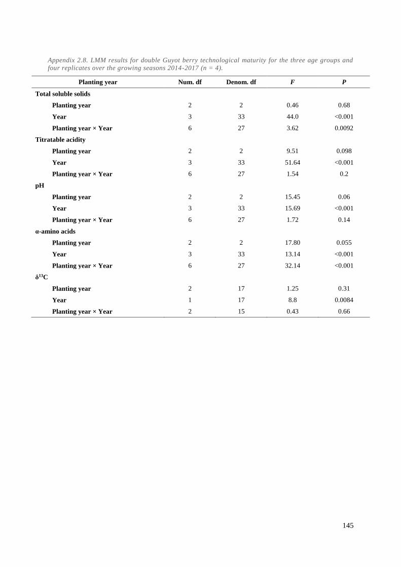
145
Appendix 2.8. LMM results for double Guyot berry technological maturity for the three age groups and
four replicates over the growing seasons 2014-2017 (n = 4).
Planting year Num. df Denom. df F P
Total soluble solids
Planting year 2 2 0.46 0.68
Year 3 33 44.0 <0.001
Planting year × Year 6 27 3.62 0.0092
Titratable acidity
Planting year 2 2 9.51 0.098
Year 3 33 51.64 <0.001
Planting year × Year 6 27 1.54 0.2
pH
Planting year 2 2 15.45 0.06
Year 3 33 15.69 <0.001
Planting year × Year 6 27 1.72 0.14
α-amino acids
Planting year 2 2 17.80 0.055
Year 3 33 13.14 <0.001
Planting year × Year 6 27 32.14 <0.001
δ13C
Planting year 2 17 1.25 0.31
Year 1 17 8.8 0.0084
Planting year × Year 2 15 0.43 0.66

146
Appendix 2.9. LMM results for the water deficit trial on cordon vines. Soil water content from 0-30 cm
and 30-60 cm (n = 4), leaf chlorophyll index (n = 8), stomatal conductance (n = 8), predawn water
potential (n = 8), and carbon isotope discrimination (n = 4). The data represents three age groups, two
water deficit treatments, and four replicates over the growing seasons 2016-2017. Three measurements
were made for soil water content per vintage (flowering, pea size, and two weeks after veraison). Six
measures were taken between 400 GDD and harvest for chlorophyll index and stomatal conductance in
2016 and seven measures in 2017, depending on weather conditions. Four measures were taken for
predawn water potential during the same period. Carbon isotope discrimination was measured on berry
samples at harvest.
Planting year Num. df Denom. df F P
Soil water at 0-30 cm
Planting year 2 134 4.60 0.012
Year 1 134 74.90 < 0.001
Water status 1 134 87.48 < 0.001
Planting year × Year 2 129 1.98 0.14
Planting year × Water status 2 129 0.95 0.39
Year × Water status 1 129 4.40 0.038
Planting year × Year × Water status 2 127 0.024 0.98
Soil water at 30-60 cm
Planting year 2 134 1.75 0.18
Year 1 134 86.38 < 0.001
Water status 1 134 34.38 < 0.001
Planting year × Year 2 129 0.0016 1
Planting year × Water status 2 129 0.69 0.51
Year × Water status 1 129 0.45 0.54
Planting year × Year × Water status 2 127 1.26 0.29
SFR_G index
Planting year 2 43 2.59 0.086
Year 1 1680 1.67 0.20
Water status 1 43 0.03 0.87
Planting year × Year 2 1677 5.67 0.0035
Planting year × Water status 2 41 0.74 0.48
Year × Water status 1 1677 3.28 0.070
Planting year × Year × Water status 2 1676 4.93 0.0073
gs
Planting year 2 571 42.92 < 0.001
Year 1 571 187.18 < 0.001
Water status 1 571 9.81 0.0018 Planting year × Year 2 566 081 0.45 Planting year × Water status 2 566 3.68 0.026 Year × Water status 1 566 4.28 0.039 Planting year × Year × Water status 2 564 3.77 0.02 ΨPD
Planting year 2 41 10.40 < 0.001
Year 1 332 51.21 < 0.001
Water status 1 41 10.39 0.0025
Planting year × Year 2 329 0.015 0.99
Planting year × Water status 2 39 2.62 0.085
Year × Water status 1 329 3.52 0.062
Planting year × Year × Water status 2 327 1.65 0.19
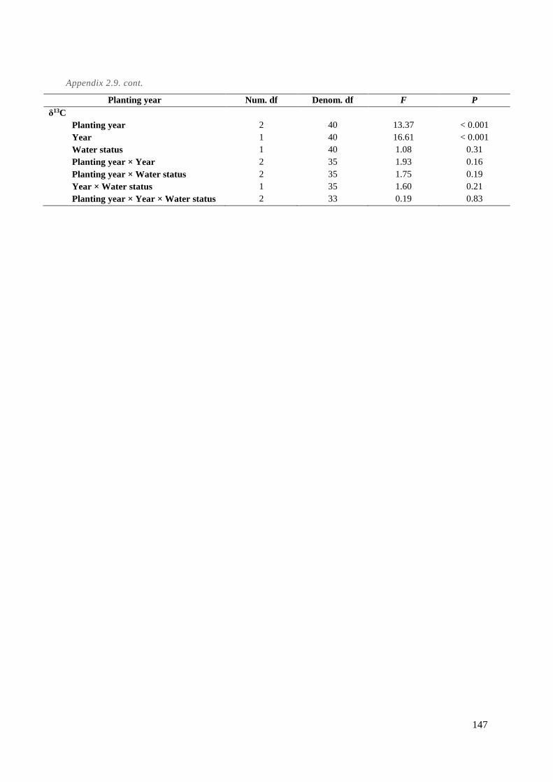
147
Appendix 2.9. cont.
Planting year Num. df Denom. df F P
δ13C
Planting year 2 40 13.37 < 0.001
Year 1 40 16.61 < 0.001
Water status 1 40 1.08 0.31
Planting year × Year 2 35 1.93 0.16
Planting year × Water status 2 35 1.75 0.19
Year × Water status 1 35 1.60 0.21
Planting year × Year × Water status 2 33 0.19 0.83

148
Appendix 3.1. Eigenvalues and eigenvectors from principal component analysis presented in Figure 3.2.
Eigenvalue PC 1 PC 2 PC 3 PC 4 PC 5 PC 6 PC 7 PC 8 PC 9
Eigenvalue 12.903 8.371 3.648 3.074 1.887 1.327 0.874 0.678 0.555
Variance (%) 35.841 23.254 10.134 8.540 5.241 3.685 2.426 1.883 1.543
Cumulative (%) 35.841 59.095 69.229 77.768 83.009 86.694 89.121 91.004 92.546
Eigenvector
SkinDryWeight -0.407 0.849 0.024 -0.020 0.124 0.014 0.127 0.122 -0.068
Fructose -0.262 0.269 0.468 0.186 0.753 -0.007 0.026 0.086 -0.107
Glucose -0.190 0.413 0.279 0.100 0.797 -0.052 0.056 0.138 -0.057
Mal -0.353 0.669 0.334 0.308 -0.301 -0.078 0.091 -0.093 0.169
Tar -0.343 0.380 0.433 -0.433 -0.255 -0.087 0.111 0.280 0.272
Asp 0.649 -0.137 -0.612 -0.283 0.133 0.071 -0.012 0.147 0.016
Glu 0.660 0.347 -0.490 -0.335 0.160 0.118 -0.051 0.138 0.049
Asn 0.654 0.543 0.312 0.155 -0.037 -0.038 -0.199 -0.043 0.045
Ser 0.828 0.341 0.044 0.211 0.184 0.230 0.032 0.022 0.148
Gly 0.214 -0.617 0.041 0.214 0.205 0.072 0.547 0.031 0.249
Gln 0.853 0.445 0.045 0.050 -0.044 0.090 -0.114 -0.009 0.019
Arg 0.806 0.341 0.198 0.249 -0.210 0.118 -0.053 -0.005 0.035
Thr 0.907 0.257 -0.023 0.140 -0.124 0.041 -0.046 0.027 0.121
Ala 0.532 -0.260 0.091 0.570 -0.147 0.373 0.220 -0.053 0.008
Pro 0.560 0.319 -0.479 0.398 0.099 0.025 0.109 -0.094 0.129
Tyr 0.830 -0.229 0.033 0.302 0.237 -0.112 -0.048 0.109 0.118
Val 0.899 0.007 0.107 0.243 -0.054 0.240 0.064 0.127 -0.133
Met 0.619 -0.055 0.106 0.492 -0.072 -0.496 -0.162 0.213 -0.078
Ileu 0.755 0.021 0.129 -0.002 -0.201 0.449 0.101 0.107 -0.275
Leu 0.575 0.258 -0.202 0.500 -0.128 -0.432 -0.066 0.199 0.068
Phe 0.470 0.729 0.314 0.089 -0.108 -0.088 -0.016 0.010 -0.190
F.Linalool 0.464 -0.788 -0.052 0.055 0.003 -0.054 -0.006 0.020 -0.266
B.Linalooloxide1 0.804 0.235 0.235 -0.309 0.106 -0.117 -0.007 -0.280 0.045
B.Neroloxide 0.718 -0.170 0.508 -0.316 -0.027 -0.177 0.058 -0.164 -0.006
B.Linalooloxide2 0.780 0.063 0.306 -0.311 0.120 -0.206 0.025 -0.259 0.017
B.Vitispirane 0.418 -0.462 0.694 -0.196 -0.097 -0.022 0.129 0.068 -0.066
B.aTerpineol 0.427 -0.795 0.284 -0.084 -0.062 -0.087 -0.003 0.121 -0.037
B.TDN 0.519 -0.641 0.370 -0.300 -0.009 -0.167 0.194 0.079 0.018
Brix -0.237 0.779 0.278 -0.027 0.064 0.278 -0.138 -0.048 0.026
pH 0.719 -0.456 -0.327 -0.189 0.112 -0.038 -0.060 -0.066 0.051
TotalAcidity -0.693 0.230 0.430 0.431 -0.118 -0.001 0.111 -0.064 -0.013
BerryWeight -0.223 -0.628 -0.264 0.512 0.143 -0.140 0.001 -0.208 0.032
NOPAFresh 0.762 0.367 -0.052 -0.136 0.219 -0.013 0.001 -0.282 -0.002
Querc.3.gal -0.408 -0.692 0.283 0.416 0.031 0.074 -0.151 -0.117 0.004
Querc.3.glucuronide -0.284 -0.686 0.340 0.268 0.094 0.224 -0.360 -0.033 0.099
Querc.3.glc 0.180 -0.608 0.364 -0.209 0.135 0.277 -0.344 0.149 0.255
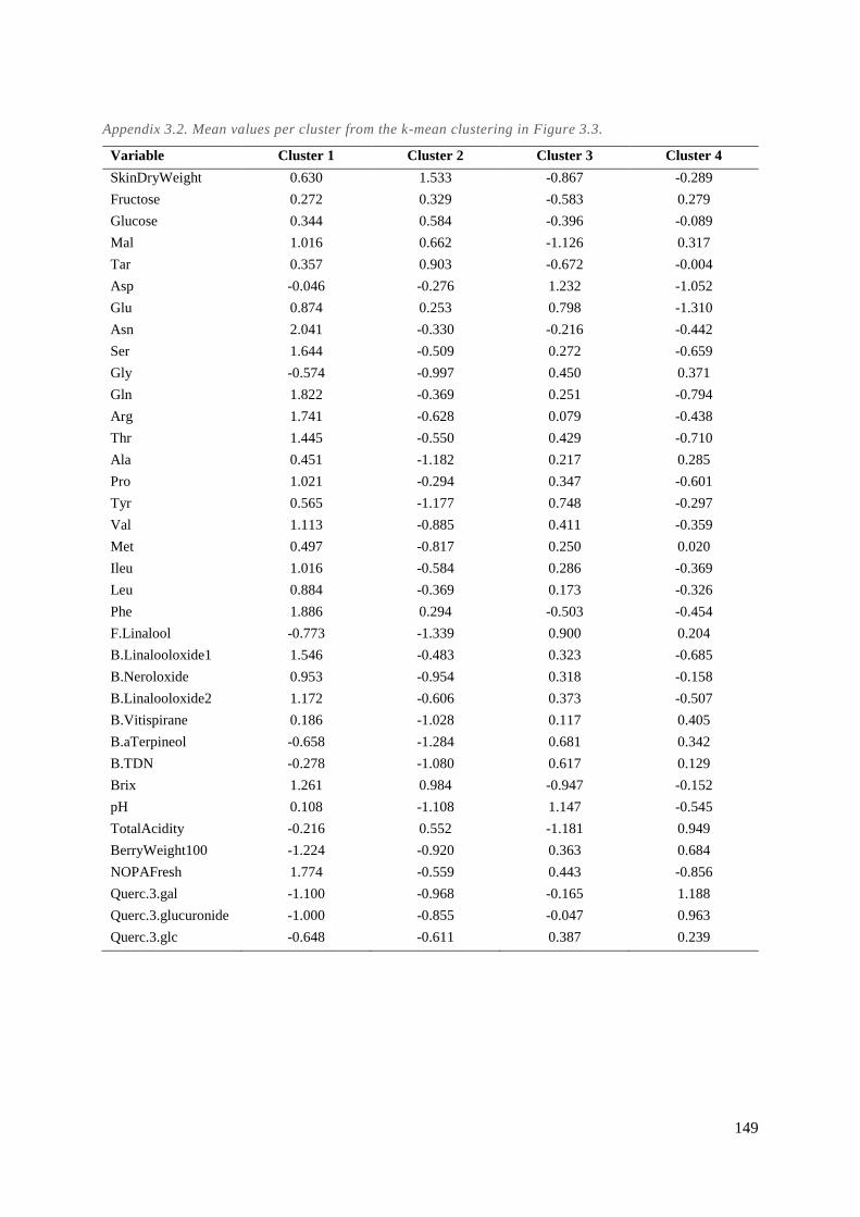
149
Appendix 3.2. Mean values per cluster from the k-mean clustering in Figure 3.3.
Variable Cluster 1 Cluster 2 Cluster 3 Cluster 4
SkinDryWeight 0.630 1.533 -0.867 -0.289
Fructose 0.272 0.329 -0.583 0.279
Glucose 0.344 0.584 -0.396 -0.089
Mal 1.016 0.662 -1.126 0.317
Tar 0.357 0.903 -0.672 -0.004
Asp -0.046 -0.276 1.232 -1.052
Glu 0.874 0.253 0.798 -1.310
Asn 2.041 -0.330 -0.216 -0.442
Ser 1.644 -0.509 0.272 -0.659
Gly -0.574 -0.997 0.450 0.371
Gln 1.822 -0.369 0.251 -0.794
Arg 1.741 -0.628 0.079 -0.438
Thr 1.445 -0.550 0.429 -0.710
Ala 0.451 -1.182 0.217 0.285
Pro 1.021 -0.294 0.347 -0.601
Tyr 0.565 -1.177 0.748 -0.297
Val 1.113 -0.885 0.411 -0.359
Met 0.497 -0.817 0.250 0.020
Ileu 1.016 -0.584 0.286 -0.369
Leu 0.884 -0.369 0.173 -0.326
Phe 1.886 0.294 -0.503 -0.454
F.Linalool -0.773 -1.339 0.900 0.204
B.Linalooloxide1 1.546 -0.483 0.323 -0.685
B.Neroloxide 0.953 -0.954 0.318 -0.158
B.Linalooloxide2 1.172 -0.606 0.373 -0.507
B.Vitispirane 0.186 -1.028 0.117 0.405
B.aTerpineol -0.658 -1.284 0.681 0.342
B.TDN -0.278 -1.080 0.617 0.129
Brix 1.261 0.984 -0.947 -0.152
pH 0.108 -1.108 1.147 -0.545
TotalAcidity -0.216 0.552 -1.181 0.949
BerryWeight100 -1.224 -0.920 0.363 0.684
NOPAFresh 1.774 -0.559 0.443 -0.856
Querc.3.gal -1.100 -0.968 -0.165 1.188
Querc.3.glucuronide -1.000 -0.855 -0.047 0.963
Querc.3.glc -0.648 -0.611 0.387 0.239

150
Appendix 3.3. Eigenvalues and eigenvectors from principal component analysis presented in Figure 3.4.
Eigenvalues PC 1 PC 2 PC 3 PC 4 PC 5 PC 6 PC 7 PC 8 PC 9
Eigenvalues 5.126 3.098 0.687 0.454 0.364 0.095 0.076 0.058 0.027
Variance (%) 51.266 30.983 6.877 4.541 3.643 0.952 0.761 0.581 0.273
Cumulative (%) 51.266 82.249 89.126 93.667 97.311 98.263 99.024 99.606 99.880
Eigenvectors
F.Linalool 0.722 0.289 -0.487 0.373 0.049 -0.087 0.002 0.084 0.005
B.Linalooloxide1 0.562 -0.764 0.176 0.184 0.157 -0.017 0.054 -0.007 0.002
B.Neroloxide 0.869 -0.428 0.109 -0.122 0.104 0.034 0.042 0.073 -0.114
B.Linalooloxide2 0.690 -0.660 0.132 0.139 0.175 0.059 -0.054 -0.059 0.077
B.Vitispirane 0.891 0.060 0.020 -0.406 0.024 -0.172 0.035 0.030 0.060
B.aTerpineol 0.881 0.312 -0.246 -0.037 -0.124 0.084 0.140 -0.141 -0.007
B.TDN 0.943 0.010 -0.161 -0.133 -0.133 0.080 -0.202 -0.006 -0.013
Querc.3.gal 0.189 0.908 0.069 -0.082 0.308 0.157 0.029 0.077 0.036
Querc.3.glucuronide 0.320 0.855 0.283 0.125 0.194 -0.119 -0.068 -0.105 -0.049
Querc.3.glc 0.675 0.391 0.465 0.197 -0.359 0.019 0.027 0.064 0.023

151
Appendix 4.1. ANOVA P-values from the sensory descriptive analysis in 2017.
Attribute
Assessor
(A) Wine (W)
Replicate
(R) A × W W × R A × R
color intensity < 0.001 < 0.001 0.624 0.001 0.046 < 0.001
citrus < 0.001 0.199 0.544 0.217 0.352 0.002
peach < 0.001 0.029 0.955 < 0.001 0.033 < 0.001
dry fruit < 0.001 < 0.001 0.240 0.009 0.015 0.583
rose < 0.001 0.508 0.003 0.054 0.624 0.043
vegetative < 0.001 0.001 0.845 0.389 0.128 < 0.001
spice < 0.001 < 0.001 0.067 0.127 0.951 0.401
aging/kerosene < 0.001 < 0.001 0.024 0.002 0.887 0.422
burnt rubber < 0.001 0.019 0.543 0.02 0.056 0.053
reductive < 0.001 < 0.001 0.984 0.001 0.773 0.007
sourness < 0.001 < 0.001 0.954 < 0.001 0.731 0.001
sweetness < 0.001 < 0.001 0.018 < 0.001 0.793 0.382
bitterness < 0.001 0.19 0.60 0.028 0.729 < 0.001
overall < 0.001 < 0.001 0.124 < 0.001 0.118 0.399
Appendix 4.2. Eigenvalues and eigenvectors from principal component analysis presented in Figure 4.1
Eigenvalue PC 1 PC 2 PC 3 PC 4 PC 5 PC 6 PC 7 PC 8
Eigenvalue 9.398 2.048 1.157 0.832 0.228 0.213 0.094 0.030
Variance (%) 67.129 14.628 8.266 5.944 1.629 1.519 0.673 0.214
Cumulative (%) 67.129 81.756 90.022 95.966 97.595 99.114 99.786 100.000
Eigenvector
Color 0.832 -0.301 -0.130 0.404 0.164 0.073 0.063 0.016
Citrus -0.472 0.838 0.099 -0.081 0.201 -0.110 0.042 -0.073
Peach 0.931 0.189 0.177 0.139 -0.178 -0.003 -0.123 0.013
DryFruit 0.992 0.003 -0.045 0.055 0.038 0.090 0.028 0.008
Rose -0.452 0.439 0.491 0.572 -0.156 0.087 0.055 -0.017
Vegetal -0.947 -0.055 0.125 0.190 0.181 -0.038 -0.029 0.116
Spices 0.756 0.539 0.119 -0.283 -0.047 0.033 0.185 0.081
Aging 0.973 -0.028 -0.225 -0.002 0.006 0.005 0.033 -0.017
Reductive -0.793 -0.520 0.084 -0.210 -0.163 0.103 0.110 -0.019
BurntRubber -0.871 -0.436 0.182 0.062 0.058 0.011 0.100 -0.028
Sourness -0.768 0.428 -0.251 -0.141 0.035 0.372 -0.071 0.007
Sweetness 0.895 -0.236 0.283 0.041 0.178 0.165 0.007 -0.046
Bitterness -0.500 0.172 -0.764 0.356 -0.071 -0.026 0.072 -0.011
Impression 0.992 0.066 -0.099 0.016 -0.030 -0.008 0.030 -0.008

152
Appendix 4.3. Concentrations of free qnd potentially volatile monoterpenes qnd norisoprenoids (μg L-1)
measured in available wines from 2002 to 2016.
Wine α-terpineol hotrienol
cis-linalool
oxide
trans-lianlool
oxide TDN
Free monoterpenes and norisoprenoids
2002-O 34.0 64.8 133.0 64.8 7.5
2002-M 37.4 63.8 122.0 60.5 8.8
2003-O 31.3 69.2 136.0 67.9 14.6
2003-M 22.1 65.3 128.2 66.4 12.4
2004-O 9.8 29.2 113.9 60.1 6.0
2004-M 10.9 33.5 117.0 59.6 10.1
2005-O 82.7 75.9 127.5 65.5 1.5
2005-M 77.2 66.7 113.7 56.0 1.6
2007-O 31.6 80.7 107.4 57.6 4.6
2007-M 27.1 68.4 124.5 63.2 6.0
2010-O 36.7 57.0 83.4 42.0 4.2
2010-M 39.3 70.3 92.6 47.7 4.8
2011-O 65.0 90.0 127.2 62.4 13.1
2011-M 59.9 83.6 121.8 63.4 9.0
2012-O 85.4 104.4 106.5 47.9 2.8
2012-M 75.0 113.4 113.3 53.3 6.4
2013-O 28.1 50.7 50.7 22.4 3.5
2013-M 24.3 59.0 57.8 26.0 5.2
2014-O 54.9 145.8 70.0 33.1 3.1
2014-M 45.9 132.2 70.0 33.5 3.4
2014-Y 28.6 125.2 56.4 25.9 3.8
2015-O 29.9 121.4 53.2 24.6 4.3
2015-M 191.9 128.6 77.1 38.2 4.5
2015-Y 60.8 107.0 66.7 28.5 5.2
2016-O 55.5 90.1 23.2 11.5 1.8
2016-M 54.7 79.7 22.7 11.4 2.1
2016-Y 73.2 62.9 23.4 11.5 1.9
Potentially volatile monoterpenes and norisoprenoids
2002-O 15.6 n.d. n.d. 10.1 6.1
2002-M 18.3 n.d. n.d. 10.8 9.0
2003-O 11.0 n.d. n.d. 9.0 7.9
2003-M 8.7 n.d. n.d. 8.3 7.3
2004-O 6.8 n.d. n.d. 9.0 0.8
2004-M 6.6 n.d. n.d. 8.4 3.4
2005-O 12.9 n.d. n.d. 9.6 3.9
2005-M 13.5 n.d. n.d. 9.1 0.7
2007-O 9.3 n.d. n.d. 8.9 0.8
2007-M 8.7 n.d. n.d. 9.1 3.7
2010-O 19.8 n.d. n.d. 9.7 7.2
2010-M 21.5 n.d. n.d. 11.5 8.6
2011-O 15.6 n.d. n.d. 10.4 11.4
2011-M 17.5 n.d. n.d. 10.5 11.2
2012-O 22.1 n.d. n.d. 7.9 6.6
2012-M 19.3 n.d. n.d. 8.3 8.3
2013-O 21.9 n.d. n.d. 7.9 9.5
2013-M 17.0 n.d. n.d. 7.9 9.6

153
Appendix 4.3. cont.
Wine α-terpineol hotrienol
cis-linalool
oxide
trans-linalool
oxide TDN
Potentially volatile monoterpenes and norisoprenoids
2014-O 23.7 n.d. n.d. 8.1 11.2
2014-M 19.7 n.d. n.d. 7.7 10.9
2014-Y 82.2 n.d. n.d. 10.1 19.6
2015-O 20.6 n.d. n.d. 8.1 9.7
2015-M 18.4 n.d. n.d. 7.8 10.1
2015-Y 38.0 n.d. n.d. 9.3 14.0
2016-O 26.9 n.d. n.d. 7.6 11.3
2016-M 28.0 n.d. n.d. 8.3 14.1
2016-Y 35.6 n.d. n.d. 8.7 17.9
Appendix 4.4. Volatile sulfur compounds (µg L-1) measured in available wines from 2002 to 2016. Only
H2S and DMS were detected in wine.
Wine H2S DMS
2002-O 7.8 31.2
2002-M 15.5 27.6
2003-O 10.2 23.5
2003-M 20.0 20.6
2004-O 24.1 36.8
2004-M 16.7 33.1
2005-O 29.0 28.3
2005-M 25.9 25.7
2007-O 32.3 28.7
2007-M 27.8 25.3
2010-O 7.8 18.4
2010-M 8.6 19.2
2011-O 17.7 15.5
2011-M 10.6 13.7
2012-O 26.4 18.8
2012-M 20.7 17.1
2013-O 24.5 16.8
2013-M 7.7 13.8
2014-O 11.8 10.2
2014-M 21.9 10.1
2014-Y 26.1 11.7
2015-O 12.0 7.3
2015-M 10.3 6.5
2015-Y 27.5 10.8
2016-O 6.4 4.2
2016-M 6.0 3.7
2016-Y 9.6 4.4

154
Appendix 4.5. Chemical compounds by 1H NMR and CIELab parameters measured in available wines from 2002 to 2016.
Wine
Butane-
diol
Phenyl-
ethanol
Methyl-
butanol
Acet-
aldehyde
Caftaric
Acid
Ethyl-
acetate
Galactu-
ronic Acid Glycerol Methanol
Succinic
Acid L* a* b*
2002-O 300 53.0 132 18.8 19.5 n.d. 467 6534 102 453 96.85 -2.50 20.04
2002-M 265 62.4 141 26.5 27.0 n.d. 478 6530 92 471 96.39 -2.29 20.82
2003-O 461 61.2 157 19.5 24.6 n.d. 362 7524 56 576 98.55 -2.17 11.71
2003-M 518 85.9 182 17.9 28.0 n.d. 343 7512 51 657 98.34 -2.01 12.11
2004-O 256 n.d. n.d. 20.9 n.d. n.d. 364 6011 87 214 98.14 -2.54 14.41
2004-M 248 n.d. n.d. 29.6 n.d. n.d. 348 5584 99 216 97.65 -2.07 15.23
2005-O 408 27.8 127 20.1 19.8 n.d. 425 8840 52 498 97.85 -2.79 16.10
2005-M 349 44.9 152 12.6 21.5 n.d. 414 8486 53 528 98.30 -2.72 14.23
2007-O 365 n.d. n.d. 38.8 n.d. n.d. 243 6659 57 263 99.41 -1.30 6.16
2007-M 279 n.d. 110 34.2 16.0 n.d. 246 6565 60 327 99.28 -1.39 6.94
2010-O 217 44.0 152 49.3 29.6 n.d. 661 7587 87 441 99.38 -1.27 6.49
2010-M 237 38.7 133 49.3 29.0 n.d. 615 7000 100 371 99.19 -1.46 7.34
2011-O 285 70.3 163 25.9 32.3 50.6 513 9302 56 570 98.78 -1.72 9.33
2011-M 264 69.4 149 31.9 40.3 52.5 463 8392 49 536 99.03 -1.55 8.16
2012-O 328 73.9 209 23.7 39.3 n.d. 525 7138 84 718 98.47 -1.97 11.31
2012-M 389 93.4 179 26.3 40.4 n.d. 493 6638 83 626 98.81 -1.86 9.59
2013-O 225 36.0 118 36.4 44.7 n.d. 475 5505 76 412 99.30 -1.45 6.77
2013-M 191 55.0 109 33.7 48.3 n.d. 451 5363 67 386 99.48 -1.23 5.50
2014-O 300 25.5 104 36.3 44.2 59.5 576 5228 63 447 99.27 -1.01 5.69
2014-M 258 27.9 108 32.0 42.4 52.0 468 5006 57 489 99.41 -0.99 4.95
2014-Y 272 31.5 127 26.6 42.7 60.1 476 6030 51 629 98.63 -1.58 9.59
2015-O 261 35.6 141 23.6 40.7 60.5 476 6165 55 660 99.14 -1.07 6.16
2015-M 261 n.d. 112 31.4 41.5 54.5 764 6126 86 504 99.27 -0.98 5.51
2015-Y 547 n.d. 100 53.4 50.7 85.6 720 8196 66 479 98.70 -1.56 9.54
2016-O 306 31.3 137 19.8 44.2 n.d. 282 5507 36 710 99.17 -1.01 5.89
2016-M 301 31.8 131 21.5 46.4 n.d. 266 5299 36 624 99.40 -0.89 4.84
2016-Y 299 31.9 125 24.1 44.5 n.d. 254 5120 36 603 99.54 -0.81 4.09

155
Appendix 4.6. Organic acids measured by HPLC (g L-1) in available wines from 2002 to 2016.
Wine
Tartaric
Acid Malic Acid
Shikimic
Acid Lactic Acid Acetic Acid Citric Acid
2002-O 1.96 2.60 52.63 0.16 0.25 0.11
2002-M 2.00 2.43 51.12 0.14 0.22 0.10
2003-O 2.41 1.27 32.66 0.11 0.28 0.11
2003-M 2.78 0.97 28.68 0.13 0.23 n.d.
2004-O 2.66 2.33 46.35 0.15 0.34 n.d.
2004-M 2.70 2.36 43.63 0.14 0.30 0.11
2005-O 1.64 1.79 37.15 0.22 0.28 n.d.
2005-M 1.67 1.65 37.10 0.23 0.26 0.13
2007-O 2.97 1.59 43.30 0.58 0.45 0.12
2007-M 2.97 1.94 45.39 0.19 0.34 0.12
2010-O 0.96 4.21 67.41 0.24 0.34 0.14
2010-M 0.98 4.64 70.71 0.18 0.29 0.14
2011-O 2.95 1.49 39.75 0.11 0.41 0.11
2011-M 3.10 1.40 39.24 n.d. 0.46 0.12
2012-O 1.88 2.16 51.37 0.16 0.30 0.14
2012-M 2.22 1.91 53.09 0.12 0.29 0.12
2013-O 1.16 3.84 58.35 n.d. 0.40 0.15
2013-M 1.82 3.74 61.02 n.d. 0.38 0.14
2014-O 2.37 2.67 57.21 0.11 0.49 0.12
2014-M 2.84 2.80 54.00 0.10 0.38 0.12
2014-Y 1.14 2.82 55.41 0.25 0.33 0.13
2015-O 3.88 3.13 55.31 0.10 0.47 0.14
2015-M 4.08 3.27 54.00 0.11 0.45 0.14
2015-Y 2.83 3.01 52.44 0.13 0.58 0.21
2016-O 3.62 2.28 44.36 0.11 0.25 0.13
2016-M 3.98 2.30 42.29 0.14 0.27 0.12
2016-Y 3.82 2.25 42.41 0.14 0.29 0.14

156
Appendix 4.7. Eigenvalues and eigenvectors from principal component analysis presented in Figure 4.2.
Eigenvalue PC 1 PC 2 PC 3 PC 4 PC 5 PC 6 PC 7 PC 8
Eigenvalue 1.938 0.598 0.373 0.283 0.185 0.125 0.052 0.020
Variance (%) 54.212 16.728 10.434 7.923 5.177 3.501 1.462 0.562
Cumulative (%) 54.212 70.940 81.374 89.297 94.475 97.976 99.438 100.000
Eigenvector
Color 0.785 -0.478 -0.019 0.063 0.337 -0.026 -0.187 0.039
Citrus -0.524 0.334 0.234 0.577 -0.434 -0.133 -0.075 0.122
Peach 0.879 -0.218 0.144 0.231 -0.222 0.176 0.032 -0.159
DryFruit 0.968 -0.134 0.053 0.176 0.085 0.047 -0.029 0.021
Rose -0.577 -0.422 0.427 0.334 -0.314 0.310 0.015 -0.016
Vegetal -0.956 -0.042 0.104 -0.142 0.046 -0.034 -0.221 -0.014
Spices 0.739 0.292 0.176 0.387 -0.333 0.177 0.042 0.207
Aging 0.965 -0.088 -0.141 0.174 0.097 -0.028 -0.012 0.032
Rubber -0.711 0.096 -0.079 -0.613 0.207 0.073 0.224 0.073
Reductive -0.837 -0.109 0.071 -0.493 0.173 -0.046 0.015 0.090
Sourness -0.769 0.450 -0.008 0.385 0.175 0.084 0.121 -0.067
Sweetness 0.886 -0.204 0.368 -0.114 0.154 -0.006 -0.027 0.016
Bitterness -0.545 -0.112 -0.638 0.457 0.258 -0.056 -0.058 0.033
Impression 0.971 -0.105 -0.045 0.208 -0.018 0.027 -0.005 0.024
Butanediol 0.620 -0.268 0.710 -0.134 0.137 0.036 -0.034 0.044
Phenylethanol -0.647 -0.403 -0.388 0.020 -0.150 0.494 0.034 -0.008
Methylbutanol -0.602 -0.367 -0.251 0.512 0.371 0.186 0.075 -0.014
Acetaldehyde 0.846 0.160 0.404 -0.290 -0.107 0.008 -0.004 0.027
CaftaricAcid 0.347 -0.412 0.776 -0.250 0.000 -0.038 -0.145 -0.150
Ethylacetate 0.918 0.267 -0.205 -0.047 -0.006 0.186 0.077 -0.019
GalacturonicAcid 0.829 0.521 -0.020 0.045 0.044 -0.182 -0.060 -0.010
Methanol 0.661 0.691 -0.126 0.061 0.012 -0.252 -0.019 -0.033
SuccinicAcid -0.538 -0.534 -0.189 0.414 0.443 0.091 0.044 0.108
L -0.798 0.468 0.210 -0.098 -0.268 0.016 0.125 -0.058
a -0.841 0.476 0.180 0.043 -0.172 0.025 0.021 -0.034
b 0.833 -0.477 -0.152 0.040 0.211 -0.033 -0.087 0.037
TartaricAcid -0.542 0.441 0.508 0.327 0.315 -0.037 0.198 -0.084
MalicAcid 0.709 0.522 -0.283 0.209 0.215 -0.001 0.225 -0.065
ShikimicAcid 0.699 0.400 -0.525 -0.027 -0.106 0.238 -0.069 0.030
LacticAcid 0.262 -0.767 -0.419 0.049 -0.186 -0.346 0.026 -0.103
AceticAcid 0.824 0.449 0.179 0.075 -0.055 0.279 0.021 -0.022
CitricAcid 0.714 -0.112 0.572 0.076 0.256 -0.054 0.221 0.165
Ethanol 0.664 0.114 0.385 0.313 0.535 0.081 -0.034 -0.080
F.Linalooloxide1 0.732 0.579 -0.293 -0.185 -0.094 -0.025 0.009 -0.013
F.Linalooloxide2 0.649 0.647 -0.334 -0.178 -0.104 -0.075 -0.005 -0.022
F.Hotrienol 0.545 0.501 -0.568 -0.171 -0.058 0.188 -0.247 -0.034
F.aTerpineol 0.034 0.627 0.159 0.235 0.044 -0.722 -0.025 0.033
F.TDN 0.887 0.298 -0.100 0.124 0.199 0.009 0.234 -0.073

157
Appendix 4.7. cont.
Eigenvector PC 1 PC 2 PC 3 PC 4 PC 5 PC 6 PC 7 PC 8
B.Linalooloxide2 0.553 -0.716 -0.109 0.152 -0.277 -0.163 0.182 -0.099
B.aTerpineol 0.350 -0.784 -0.398 0.071 -0.180 -0.254 0.035 0.028
B.TDN 0.078 -0.807 -0.054 0.050 -0.422 -0.334 0.217 0.003
H2S 0.797 -0.268 -0.205 -0.393 -0.026 0.009 0.304 0.058
DMS 0.812 -0.022 -0.383 -0.337 -0.214 0.178 0.013 0.049
Appendix 4.8. Eigenvalues and eigenvectors from principal component analysis presented in Figure 4.4.
Eigenvalue PC 1 PC 2 PC 3 PC 4 PC 5 PC 6 PC 7 PC 8 PC 9
Eigenvalue 9.021 5.312 3.408 2.872 1.809 1.646 1.483 1.078 0.749
Variance (%) 30.069 17.707 11.360 9.572 6.031 5.486 4.943 3.593 2.498
Cumulative (%) 30.069 47.776 59.135 68.707 74.739 80.225 85.168 88.761 91.259
Eigenvector
Butanediol -0.268 -0.564 0.049 0.338 0.161 0.293 0.068 0.294 -0.209
Phenylethanol -0.150 -0.408 0.466 -0.531 0.423 -0.017 0.211 0.059 0.055
Methylbutanol 0.167 -0.547 0.565 -0.399 0.202 -0.008 0.293 -0.014 -0.130
Acetaldehyde 0.382 0.670 0.230 0.323 0.231 0.041 -0.026 0.061 -0.301
CaftaricAcid 0.824 -0.281 0.309 -0.159 0.126 0.082 0.113 0.087 0.172
Ethylacetate 0.505 -0.142 0.331 0.649 0.102 0.069 -0.280 0.020 0.206
GalacturonicAcid 0.296 0.243 0.786 0.326 -0.060 -0.149 0.144 0.205 0.068
Methanol -0.361 0.595 0.466 -0.011 -0.256 -0.311 0.048 0.222 0.038
SuccinicAcid 0.365 -0.809 0.271 -0.277 0.028 0.069 0.110 0.033 -0.016
L 0.733 0.099 -0.355 0.099 0.329 -0.024 0.271 -0.027 -0.279
a 0.884 0.089 -0.263 0.024 0.164 -0.214 -0.067 -0.017 -0.143
b -0.825 -0.075 0.336 -0.082 -0.284 0.082 -0.170 0.023 0.234
TartaricAcid 0.267 -0.472 -0.502 0.321 0.032 -0.467 -0.197 -0.018 0.127
MalicAcid 0.506 0.708 0.278 -0.171 -0.217 -0.070 0.028 0.178 -0.012
ShikimicAcid 0.485 0.682 0.405 -0.114 -0.205 -0.057 0.063 0.112 -0.081
LacticAcid 0.111 0.547 -0.216 -0.218 0.295 0.376 0.391 -0.084 0.391
AceticAcid 0.462 0.248 0.043 0.744 0.272 0.041 0.026 0.000 0.212
CitricAcid -0.359 -0.117 -0.227 0.054 0.134 0.110 -0.060 0.770 -0.027
Ethanol -0.548 -0.491 0.250 0.444 -0.062 0.058 0.188 -0.139 0.093
F.Linalooloxide1 -0.870 -0.020 0.287 0.205 0.213 -0.110 0.080 -0.089 -0.087
F.Linalooloxide2 -0.884 -0.005 0.217 0.203 0.224 -0.130 0.048 -0.098 -0.117
F.Hotrienol 0.596 -0.369 0.321 0.411 -0.113 0.008 0.078 -0.047 -0.068
F.aTerpineol 0.300 -0.338 0.266 0.309 -0.264 -0.343 0.397 -0.186 0.035
F.TDN -0.510 -0.125 0.178 0.040 0.599 -0.256 -0.336 0.134 0.116
B.Linalooloxide2 -0.351 0.225 0.511 -0.054 0.186 0.117 -0.447 -0.346 -0.242
B.aTerpineol 0.577 -0.127 0.268 -0.089 -0.217 0.546 -0.378 -0.052 -0.019
B.TDN 0.755 -0.271 0.231 -0.159 0.100 0.156 -0.416 0.003 0.088
H2S -0.342 0.005 -0.100 0.480 -0.117 0.650 0.269 -0.014 -0.093
DMS -0.928 0.329 -0.021 0.049 -0.097 0.079 0.010 -0.008 -0.017

158
References
Agisoft LLC, 2014. Sample Data [WWW Document]. Agisoft Sample Data. URL
http://www.agisoft.com/downloads/sample-data/ (accessed 9.17.18).
Algarra Alarcon, A., Lazazzara, V., Cappellin, L., Bianchedi, P.L., Schuhmacher, R., Wohlfahrt,
G., Pertot, I., Biasioli, F., Perazzolli, M., 2015. Emission of volatile sesquiterpenes and
monoterpenes in grapevine genotypes following Plasmopara viticola inoculation in vitro. J.
Mass Spectrom. 50, 1013–1022. https://doi.org/10.1002/jms.3615
Allen, D.J., Ort, D.R., 2001. Impacts of chilling temperatures on photosynthesis in warm-climate
plants. Trends Plant Sci. 6, 36–42. https://doi.org/10.1016/S1360-1385(00)01808-2
Ambrosi, H., 2011. Farbatlas Rebsorten - 300 Sorten und ihre Weine. Ulmer, Stuttgart.
Archer, E., Strauss, H.C., 1985. Effect of Plant Density on Root Distribution of Three-Year-Old
Grafted 99 Richter Grapevines. South Afr. J. Enol. Vitic. 6, 25–30.
https://doi.org/10.21548/6-2-2347
Austin, C.N., Grove, G.G., Meyers, J.M., Wilcox, W.F., 2011. Powdery Mildew Severity as a
Function of Canopy Density: Associated Impacts on Sunlight Penetration and Spray
Coverage. Am. J. Enol. Vitic. 62, 23–31. https://doi.org/10.5344/ajev.2010.10077
Austin, C.N., Lakso, A.N., Seem, R.C., Riegel, D.G., Wilcox, W.F., 2009. Inhibition of powdery
mildew by improved vineyard sunlight exposure. Abstr. Am. J. Enol. Vitic. 60, 369A.
Bakker, J., Clarke, R.J., 2011. Wine: flavour chemistry. John Wiley & Sons.
Barossa Chapters, 2018. Barossa Chapters: Old Vines [WWW Document]. Barossa Wine. URL
https://www.barossawine.com/barossa/barossa-chapters/barossa-chapters-old-vines/ (accessed
2.22.18).
Bauerle, T.L., Richards, J.H., Smart, D.R., Eissenstat, D.M., 2008. Importance of internal
hydraulic redistribution for prolonging the lifespan of roots in dry soil. Plant Cell Environ. 31,
177–186. https://doi.org/10.1111/j.1365-3040.2007.01749.x
Bavaresco, L., Gatti, M., Pezzutto, S., Fregoni, M., Mattivi, F., 2008. Effect of Leaf Removal on
Grape Yield, Berry Composition, and Stilbene Concentration. Am. J. Enol. Vitic. 59, 292–
298.
Beis, A., Patakas, A., 2015. Differential physiological and biochemical responses to drought in
grapevines subjected to partial root drying and deficit irrigation. Eur. J. Agron. 62, 90–97.
https://doi.org/10.1016/j.eja.2014.10.001

159
Bell, S.-J., Henschke, P.A., 2005. Implications of nitrogen nutrition for grapes, fermentation and
wine. Aust. J. Grape Wine Res. 11, 242–295. https://doi.org/10.1111/j.1755-
0238.2005.tb00028.x
Bernizzoni, F., Gatti, M., Civardi, S., Poni, S., 2009. Long-term Performance of Barbera Grown
under Different Training Systems and Within-Row Vine Spacings. Am. J. Enol. Vitic. 60,
339–348.
Bindon, K.A., Dry, P.R., Loveys, B.R., 2007. Influence of Plant Water Status on the Production
of C13-Norisoprenoid Precursors in Vitis vinifera L. Cv. Cabernet Sauvignon Grape Berries.
J. Agric. Food Chem. 55, 4493–4500. https://doi.org/10.1021/jf063331p
Bisson, L.F., Waterhouse, A.L., Ebeler, S.E., Walker, M.A., Lapsley, J.T., 2002. The present and
future of the international wine industry. Nature 418, 696.
Black, C. a., Parker, M., Siebert, T. e., Capone, D. l., Francis, I. l., 2015. Terpenoids and their
role in wine flavour: recent advances. Aust. J. Grape Wine Res. 21, 582–600.
https://doi.org/10.1111/ajgw.12186
Bou Nader, K., Stoll, M., Rauhut, D., Patz, C.-D., Jung, R., Loehnertz, O., Schultz, H.R., Hilbert,
G., Renaud, C., Roby, J.-P., Delrot, S., Gomès, E., 2019. Impact of grapevine age on water
status and productivity of Vitis vinifera L. cv. Riesling. Eur. J. Agron. 104, 1–12.
https://doi.org/10.1016/j.eja.2018.12.009
Bou Nader, K., Stoll, M., Rauhut, D., Patz, C.-D., Jung, R., Löhnertz, O., Schultz, H.R., Hilbert,
G., Renaud, C., Roby, J.-P., Delrot, S., Gomès, E., n.d. Impact of Grapevine Age on Water
Stress Tolerance and Productivity of Vitis vinifera L. cv. Riesling. Eur. J. Agron.
Boursiquot, J., Lacombe, T., Bowers, J., Meredith, C., 2004. Le Gouais, un cépage clé du
patrimoine viticole européen. Bull. L’OIV 77, 5–19.
Braam, J., 2005. In touch: plant responses to mechanical stimuli. New Physiol. 165, 373–389.
Brady, N.C., Weil, R.R., 2002. The nature and properties of soils. Prentice Hall, Upper Saddle
River.
Brodersen, C.R., McElrone, A.J., Choat, B., Matthews, M.A., Shackel, K.A., 2010. The
dynamics of embolism repair in xylem: in vivo visualizations using High Resolution
Computed Tomography. Plant Physiol. pp.110.162396.
https://doi.org/10.1104/pp.110.162396
Bruwer, J., Fong, M., Saliba, A., 2013. Perceived risk, risk-reduction strategies (RRS) and
consumption occasions: Roles in the wine consumer’s purchase decision. Asia Pac. J. Mark.
Logist. 25, 369–390. https://doi.org/10.1108/APJML-06-2012-0048

160
Cadot, Y., Miñana-Castelló, M.T., Chevalier, M., 2006. Anatomical, Histological, and
Histochemical Changes in Grape Seeds from Vitis vinifera L. cv Cabernet franc during Fruit
Development. J. Agric. Food Chem. 54, 9206–9215. https://doi.org/10.1021/jf061326f
Canuti, V., Picchi, M., Zanoni, B., Fia, G., Bertuccioli, M., 2017. A Multivariate Methodological
Approach to Relate Wine to Characteristics of Grape Composition: The Case of Typicality.
Am. J. Enol. Vitic. 68, 49–59. https://doi.org/10.5344/ajev.2016.15111
Castillo-Muñoz, N., Gómez-Alonso, S., García-Romero, E., Hermosín-Gutiérrez, I., 2010.
Flavonol profiles of Vitis vinifera white grape cultivars. J. Food Compos. Anal. 23, 699–705.
https://doi.org/10.1016/j.jfca.2010.03.017
Celette, F., Gaudin, R., Gary, C., 2008. Spatial and temporal changes to the water regime of a
Mediterranean vineyard due to the adoption of cover cropping. Eur. J. Agron. 29, 153–162.
https://doi.org/10.1016/j.eja.2008.04.007
Champagnol, F., 1984. Elements de Physiologie de la Vigne et de Viticulture Generale, F.
Champagnol. Champagnol, Montpellier.
Charters, S., Pettigrew, S., 2007. The dimensions of wine quality. Food Qual. Prefer. 18, 997–
1007. https://doi.org/10.1016/j.foodqual.2007.04.003
Chaves, M.M., Santos, T.P., Souza, C.R., Ortuño, M.F., Rodrigues, M.L., Lopes, C.M., Maroco,
J.P., Pereira, J.S., 2007. Deficit irrigation in grapevine improves water-use efficiency while
controlling vigour and production quality. Ann. Appl. Biol. 150, 237–252.
https://doi.org/10.1111/j.1744-7348.2006.00123.x
Chaves, M.M., Zarrouk, O., Francisco, R., Costa, J.M., Santos, T., Regalado, A.P., Rodrigues,
M.L., Lopes, C.M., 2010. Grapevine under deficit irrigation: hints from physiological and
molecular data. Ann. Bot. 105, 661–676. https://doi.org/10.1093/aob/mcq030
Chellemi, D.O., Marois, J.J., 1992. Influence of Leaf Removal, Fungicide Applications, and
Fruit Maturity on Incidence and Severity of Grape Powdery Mildew. Am. J. Enol. Vitic. 43,
53–57.
Chiarawipa, R., Wang, Y., Zhang, X.Z., Han, Z.H., 2013. Growing Season Carbon Dynamics
and Stocks in Relation to Vine Ages under a Vineyard Agroecosystem in Northern China.
Am. J. Plant Physiol. 8, 1–16. https://doi.org/10.3923/ajpp.2013.1.16
CIE, 1986. Colorimetry, 2nd ed, Publication. Commission Internationale de l’Eclairage, Vienna.
Cola, G., Failla, O., Mariani, L., 2009. BerryTone—A simulation model for the daily course of
grape berry temperature. Agric. For. Meteorol. 149, 1215–1228.
https://doi.org/10.1016/j.agrformet.2009.01.007
161
Collins, C., Rawnsley, B., 2005. Factors influencing primary bud necrosis (PBN) in Australian
vineyards. Acta Hortic. 81–86. https://doi.org/10.17660/ActaHortic.2005.689.5
Conde, C., Silva, P., Fontes, N., Dias, A.C.P., Tavares, R.M., Sousa, M.J., Agasse, A., Delrot, S.,
Gerós, H., 2007. Biochemical changes throughout grape berry development and fruit and
wine quality.
Considine, J.A., 2004. Grapevine productivity and yield components: A case study using field
vines of Zante currant. Aust. J. Grape Wine Res. 10, 108–115. https://doi.org/10.1111/j.1755-
0238.2004.tb00013.x
Coombe, B.G., 1995. Growth Stages of the Grapevine: Adoption of a system for identifying
grapevine growth stages. Aust. J. Grape Wine Res. 1, 104–110.
https://doi.org/10.1111/j.1755-0238.1995.tb00086.x
Coombe, B.G., 1987. Distribution of Solutes within the Developing Grape Berry in Relation to
Its Morphology. Am. J. Enol. Vitic. 38, 120–127.
Coombe, B.G., McCarthy, M.G., 2000. Dynamics of grape berry growth and physiology of
ripening. Aust. J. Grape Wine Res. 6, 131–135. https://doi.org/10.1111/j.1755-
0238.2000.tb00171.x
Correia, M.J., Chaves, M.M.C., Pereira, J.S., 1990. Afternoon Depression In Photosynthesis in
Grapevine Leaves—Evidence for a High Light Stress Effect. J. Exp. Bot. 41, 417–426.
https://doi.org/10.1093/jxb/41.4.417
Cortell, J.M., Kennedy, J.A., 2006. Effect of Shading on Accumulation of Flavonoid Compounds
in (Vitis vinifera L.) Pinot Noir Fruit and Extraction in a Model System. J. Agric. Food Chem.
54, 8510–8520. https://doi.org/10.1021/jf0616560
Credi, R., Babini, A.R., 1997. Effects of Virus and Virus-Like Infections on Growth, Yield, and
Fruit Quality of Albana and Trebbiano Romagnolo Grapevines. Am. J. Enol. Vitic. 48, 7–12.
Crosby, P.B., 1979. Quality is free: The art of marketing quality certain. New American Library,
New York, NY.
Curzi, D., Pacca, L., 2015. Price, quality and trade costs in the food sector. Food Policy 55, 147–
158. https://doi.org/10.1016/j.foodpol.2015.06.007
Daudet, F.-A., Améglio, T., Cochard, H., Archilla, O., Lacointe, A., 2005. Experimental analysis
of the role of water and carbon in tree stem diameter variations. J. Exp. Bot. 56, 135–144.
https://doi.org/10.1093/jxb/eri026
David, E., Serrano, E., Renard, R., 2001. Vigne et qualité de vendage: Effet de l’enherbement
semé. Phytoma 544, 46–47.

162
Davies, M., Smith, K., Vinten, A., 2001. The mineralisation and fate of nitrogen following
ploughing of grass and grass-clover swards. Biol. Fertil. Soils 33, 423–434.
https://doi.org/10.1007/s003740100348
Davies, W.J., Blackman, P.G., Lodge, T.R., Rosa da Costa, A., Metcalfe, J., 1987. Root to shoot
communication of the effects of soil drying, flooding or increase salinity. A case for the
involvement of plant growth regulators in a multiple chemical signal, in: Tenhunen, J.D.,
Catarino, F.M., Lange, O.L., Oechel, W.C. (Eds.), Plant Response to Stress, NATO ASI
Series. Springer Berlin Heidelberg, pp. 201–221.
De Santis, D., Frangipane, M.T., Brunori, E., Cirigliano, P., Biasi, R., 2017. Biochemical
Markers for Enological Potentiality in a Grapevine Aromatic Variety under Different Soil
Types. Am. J. Enol. Vitic. 68, 100–111. https://doi.org/10.5344/ajev.2016.15123
Delas, J., 2010. Fertilisation de la vigne: contribution à une viticulture durable. Éd. Féret,
Bordeaux.
Deloire, A., 2012. A few thoughts on grapevine training systems. Wineland Mag. 274, 82–86.
Deluc, L.G., Quilici, D.R., Decendit, A., Grimplet, J., Wheatley, M.D., Schlauch, K.A.,
Mérillon, J.-M., Cushman, J.C., Cramer, G.R., 2009. Water deficit alters differentially
metabolic pathways affecting important flavor and quality traits in grape berries of Cabernet
Sauvignon and Chardonnay. BMC Genomics 10, 212. https://doi.org/10.1186/1471-2164-10-
212
Deutsches Weininstitut, 2017. Riesling [WWW Document]. Wines Ger. URL
https://www.germanwines.de/knowledge/grape-varieties/white-grapes/riesling/ (accessed
10.6.18).
Diago, M.P., Ayestarán, B., Guadalupe, Z., Poni, S., Tardáguila, J., 2012. Impact of Prebloom
and Fruit Set Basal Leaf Removal on the Flavonol and Anthocyanin Composition of
Tempranillo Grapes. Am. J. Enol. Vitic. 63, 367–376.
https://doi.org/10.5344/ajev.2012.11116
Dimopoulou, M., Lonvaud-Funel, A., Dols-Lafargue, M., 2017. Polysaccharide Production by
Grapes Must and Wine Microorganisms, in: Biology of Microorganisms on Grapes, in Must
and in Wine. Springer, Cham, pp. 293–314. https://doi.org/10.1007/978-3-319-60021-5_12
Dokoozlian, N.K., Kliewer, W.M., 1995. The Light Environment Within Grapevine Canopies. II.
Influence of Leaf Area Density on Fruit Zone Light Environment and Some Canopy
Assessment Parameters. Am. J. Enol. Vitic. 46, 219–226.
Doster, M.A., Schnathorst, W.C., 1985. Comparative Susceptibility of Various Grapevine
Cultivars to the Powdery Mildew Fungus Uncinula Necator. Am. J. Enol. Vitic. 36, 101–104.

163
Douglas, D., Cliff, M.A., Reynolds, A.G., 2001. Canadian terroir: characterization of Riesling
wines from the Niagara Peninsula. Food Res. Int. 34, 559–563.
https://doi.org/10.1016/S0963-9969(01)00071-0
Downey, M.O., Dokoozlian, N.K., Krstic, M.P., 2006. Cultural Practice and Environmental
Impacts on the Flavonoid Composition of Grapes and Wine: A Review of Recent Research.
Am. J. Enol. Vitic. 57, 257–268.
Dry, P., Iland, P., Ristic, R., 2004. What is vine balance?, in: Proceedings of the 12th Australian
Wine Industry Technical Conference. Presented at the Australian Wine Industry Technical
Conference, Melbourne, pp. 68–74.
Dry, P, Iland, P., Ristic, R., 2004. What is vine balance? Australian Wine Industry Technical
Conference.
Dry, P. r., Loveys, B. r., 1998. Factors influencing grapevine vigour and the potential for control
with partial rootzone drying. Aust. J. Grape Wine Res. 4, 140–148.
https://doi.org/10.1111/j.1755-0238.1998.tb00143.x
Du, G., Zhan, J., Li, J., You, Y., Zhao, Y., Huang, W., 2012. Effect of Grapevine Age on the
Aroma Compounds in “Beihong” Wine. Afr J Enol Vitic 33, 7–13.
Duarte Alonso, A., Northcote, J., 2009. Wine, history, landscape: origin branding in Western
Australia. Br. Food J. 111, 1248–1259. https://doi.org/10.1108/00070700911001068
Duchêne, E., Butterlin, G., Claudel, P., Dumas, V., Jaegli, N., Merdinoglu, D., 2009. A
grapevine (Vitis vinifera L.) deoxy-d-xylulose synthase gene colocates with a major
quantitative trait loci for terpenol content. Theor. Appl. Genet. 118, 541–552.
https://doi.org/10.1007/s00122-008-0919-8
Duthie, J., Munkvold, G., Marois, J., Grant, S., Chellemi, D., 1991. Relationship between age of
vineyard and incidence of Eutypa dieback. Phytopathology 81, 1183.
Emanuelli, F., Battilana, J., Costantini, L., Le Cunff, L., Boursiquot, J.-M., This, P., Grando,
M.S., 2010. A candidate gene association study on muscat flavor in grapevine (Vitis
viniferaL.). BMC Plant Biol. 10, 241. https://doi.org/10.1186/1471-2229-10-241
Evans, J.R., 1989. Photosynthesis and nitrogen relationships in leaves of C3 plants. Oecologia
78, 9–19. https://doi.org/10.1007/BF00377192
Ezzili, B., 1992. Effect of the vine age on the evolution of the number of flower buds of Alicante
Grenache noir grown in El Khanguet (Tunisia) [fruit set, flower abscission]. Bull. OIV Fr.
Ferree, D.C., Streeter, J.G., 2004. Response of Container-grown Grapevines to Soil Compaction.
HortScience 39, 1250–1254. https://doi.org/10.21273/HORTSCI.39.6.1250

164
Filippetti, I., Intrieri, C., 2001. Planting density and physiological balance: Comparing
approaches to European viticulture in the 21st century, in: Proceedings of the ASEV 50th
Anniversary Annual Meeting, Seattle, Washington, June 19-23, 2000. American Society for
Enology and Viticulture, ASEV, pp. 296–308.
Fischer, U., Roth, D., Christmann, M., 1999. The impact of geographic origin, vintage and wine
estate on sensory properties of Vitis vinifera cv. Riesling wines. Food Qual. Prefer. 10, 281–
288. https://doi.org/10.1016/S0950-3293(99)00008-7
Flamini, R., Mattivi, F., Rosso, M.D., Arapitsas, P., Bavaresco, L., 2013. Advanced Knowledge
of Three Important Classes of Grape Phenolics: Anthocyanins, Stilbenes and Flavonols. Int. J.
Mol. Sci. 14, 19651–19669. https://doi.org/10.3390/ijms141019651
Friedel, M., Frotscher, J., Nitsch, M., Hofmann, M., Bogs, J., Stoll, M., Dietrich, H., 2016. Light
promotes expression of monoterpene and flavonol metabolic genes and enhances flavour of
winegrape berries (Vitis vinifera L. cv. Riesling). Aust. J. Grape Wine Res. 22, 409–421.
https://doi.org/10.1111/ajgw.12229
Friedel, M., Stoll, M., Patz, C., Will, F., Dietrich, H., 2015. Impact of light exposure on fruit
composition of white’Riesling’grape berries (Vitis vinifera L.). VITIS-J. Grapevine Res. 54,
107–116.
Gadoury, D.M., Seem, R.C., Ficke, A., Wilcox, W.F., 2003. Ontogenic Resistance to Powdery
Mildew in Grape Berries. Phytopathology 93, 547–555.
https://doi.org/10.1094/PHYTO.2003.93.5.547
Gambetta, G.A., Fei, J., Rost, T.L., Knipfer, T., Matthews, M.A., Shackel, K.A., Walker, M.A.,
McElrone, A.J., 2013. Water uptake along the length of grapevine fine roots: developmental
anatomy, tissue specific aquaporin expression, and pathways of water transport. Plant Physiol.
pp.113.221283. https://doi.org/10.1104/pp.113.221283
García, E., Chacón, J.L., Martínez, J., Izquierdo, P.M., 2003. Changes in Volatile Compounds
during Ripening in Grapes of Airén, Macabeo and Chardonnay White Varieties Grown in La
Mancha Region (Spain). Food Sci. Technol. Int. 9, 33–41.
https://doi.org/10.1177/1082013203009001006
Gaudillère, J.-P., Van Leeuwen, C., Ollat, N., 2002. Carbon isotope composition of sugars in
grapevine, an integrated indicator of vineyard water status. J. Exp. Bot. 53, 757–763.
https://doi.org/10.1093/jexbot/53.369.757
Gershenzon, J., Dudareva, N., 2007. The function of terpene natural products in the natural
world. Nat. Chem. Biol. 3, 408–414. https://doi.org/10.1038/nchembio.2007.5

165
Giese, G., Wolf, T.K., Velasco-Cruz, C., Roberts, L., Heitman, J., 2015. Cover Crop and Root
Pruning Impacts on Vegetative Growth, Crop Yield Components, and Grape Composition of
Cabernet Sauvignon. Am. J. Enol. Vitic. 66, 212–226.
https://doi.org/10.5344/ajev.2014.14100
Gladstones, J., 2011. Wine, terroir and climate change. Wakefield Press, Adelaide.
Godelmann, R., Fang, F., Humpfer, E., Schütz, B., Bansbach, M., Schäfer, H., Spraul, M., 2013.
Targeted and Nontargeted Wine Analysis by 1H NMR Spectroscopy Combined with
Multivariate Statistical Analysis. Differentiation of Important Parameters: Grape Variety,
Geographical Origin, Year of Vintage. J. Agric. Food Chem. 61, 5610–5619.
https://doi.org/10.1021/jf400800d
Godelmann, R., Kost, C., Patz, C.-D., Ristow, R., Wachter, H., 2016. Quantitation of
Compounds in Wine Using 1H NMR Spectroscopy: Description of the Method and
Collaborative Study. J. AOAC Int. 99, 1295–1304. https://doi.org/10.5740/jaoacint.15-0318
Goode, J., 2005. Wine science. Lond. Mitchell Beazley.
Granett, J., Walker, M.A., Kocsis, L., Omer, A.D., 2001. Biology and management of grape
phylloxera. Annu. Rev. Entomol. 46, 387–412.
Greer, D.H., 2018. The short-term temperature-dependency of CO2 photosynthetic responses of
two Vitis vinifera cultivars grown in a hot climate. Environ. Exp. Bot. 147, 125–137.
https://doi.org/10.1016/j.envexpbot.2017.11.012
Greer, D.H., Weedon, M.M., 2012. Modelling photosynthetic responses to temperature of
grapevine (Vitis vinifera cv. Semillon) leaves on vines grown in a hot climate. Plant Cell
Environ. 35, 1050–1064. https://doi.org/10.1111/j.1365-3040.2011.02471.x
Grigg, D., Methven, D., de Bei, R., Rodríguez López, C.M., Dry, P., Collins, C., 2017. Effect of
vine age on vine performance of Shiraz in the Barossa Valley, Australia. Aust. J. Grape Wine
Res. 75–87. https://doi.org/10.1111/ajgw.12312
Grigg, D.P., 2017. An investigation into the effect of grapevine age on vine performance, grape
and wine composition, sensory evaluation and epigenetic characterisation.
https://doi.org/10.25909/5b3d6e8347ffc
Gubler, W.D., Marois, J.J., Bledsoe, A.M., Bettiga, L.J., 1987. Control of Botrytis bunch rot.
Plant Dis. 71, 599–601.
Guerra, B., Steenwerth, K., 2011. Influence of Floor Management Technique on Grapevine
Growth, Disease Pressure, and Juice and Wine Composition: A Review. Am. J. Enol. Vitic.
ajev.2011.10001. https://doi.org/10.5344/ajev.2011.10001

166
Günata, Y., Bayonove, C., Baumes, R., Cordonnier, R., 1985. The aroma of grapes I. Extraction
and determination of free and glycosidically bound fractions of some grape aroma
components. J. Chromatogr. A 331, 83–90.
Habran, A., Commisso, M., Helwi, P., Hilbert, G., Negri, S., Ollat, N., Gomès, E., van Leeuwen,
C., Guzzo, F., Delrot, S., 2016. Roostocks/Scion/Nitrogen Interactions Affect Secondary
Metabolism in the Grape Berry. Front. Plant Sci. 7. https://doi.org/10.3389/fpls.2016.01134
Hart, S.C., Stark, J.M., Davidson, E.A., Firestone, M.K., 1994. Nitrogen Mineralization,
Immobilization, and Nitrification. Methods Soil Anal. Part 2—Microbiological Biochem.
Prop. sssabookseries, 985–1018. https://doi.org/10.2136/sssabookser5.2.c42
Hartigan, J.A., Wong, M.A., 1979. Algorithm AS 136: A K-Means Clustering Algorithm. J. R.
Stat. Soc. Ser. C Appl. Stat. 28, 100–108. https://doi.org/10.2307/2346830
Haselgrove, K., Botting, D., van Heeswijck, R., Hoj, P.B., Dry, P.R., Ford, C., 2000. Canopy
microclimate and berry composition: the effect of bunch exposure on the phenolic
composition of Vitis vinifera L. cv. Shiraz grape berries. Aust. J. Grape Wine Res. 6, 141–
149.
Hatch, T.A., Hickey, C.C., Wolf, T.K., 2011. Cover Crop, Rootstock, and Root Restriction
Regulate Vegetative Growth of Cabernet Sauvignon in a Humid Environment. Am. J. Enol.
Vitic. 62, 298–311. https://doi.org/10.5344/ajev.2011.11001
Helwi, P., Guillaumie, S., Thibon, C., Keime, C., Habran, A., Hilbert, G., Gomes, E., Darriet, P.,
Delrot, S., van Leeuwen, C., 2016. Vine nitrogen status and volatile thiols and their
precursors from plot to transcriptome level. BMC Plant Biol. 16, 173.
https://doi.org/10.1186/s12870-016-0836-y
Heymann, H., Noble, A.C., 1987. Descriptive Analysis of Commercial Cabernet Sauvignon
Wines from California. Am. J. Enol. Vitic. 38, 41–44.
Hilbert, G., Soyer, J., Molot, C., Giraudon, J., Milin, S., Gaudillère, J.-P., 2003. Effects of
nitrogen supply on must quality and anthocyanin accumulation in berries of cv. Merlot. Vitis
42, 69–76.
Hilbert, G., Temsamani, H., Bordenave, L., Pedrot, E., Chaher, N., Cluzet, S., Delaunay, J.-C.,
Ollat, N., Delrot, S., Mérillon, J.-M., Gomès, E., Richard, T., 2015. Flavonol profiles in
berries of wild Vitis accessions using liquid chromatography coupled to mass spectrometry
and nuclear magnetic resonance spectrometry. Food Chem. 169, 49–58.
https://doi.org/10.1016/j.foodchem.2014.07.079
Historic Vineyard Society, 2018. Historic Vineyard Society [WWW Document]. Hist. Vineyard
Soc. URL https://historicvineyardsociety.org/ (accessed 2.22.18).

167
Hochberg, U., Rockwell, F.E., Holbrook, N.M., Cochard, H., 2018. Iso/Anisohydry: A Plant–
Environment Interaction Rather Than a Simple Hydraulic Trait. Trends Plant Sci. 23, 112–
120. https://doi.org/10.1016/j.tplants.2017.11.002
Holbrook, M.B., Corfman, K.P., 1985. Quality and value in the consumption experience:
Phaedrus rides again. Perceived Qual. 31, 31–57.
Holzapfel, B.P., Smith, J.P., Field, S.K., Hardie, W.J., others, 2010. Dynamics of Carbohydrate
Reserves in Cultivated Grapevines. Hortic. Rev. 37, 143.
Hopfer, H., Heymann, H., 2014. Judging wine quality: Do we need experts, consumers or trained
panelists? Food Qual. Prefer. 32, Part C, 221–233.
https://doi.org/10.1016/j.foodqual.2013.10.004
Houghton, R.A., 2005. Aboveground Forest Biomass and the Global Carbon Balance. Glob.
Change Biol. 11, 945–958. https://doi.org/10.1111/j.1365-2486.2005.00955.x
Howell, G.S., 2001. Sustainable Grape Productivity and the Growth-Yield Relationship: A
Review. Am. J. Enol. Vitic. 52, 165–174.
Hsiao, T.C., Xu, L.-K., 2000. Sensitivity of growth of roots versus leaves to water stress:
biophysical analysis and relation to water transport. J. Exp. Bot. 51, 1595–1616.
https://doi.org/10.1093/jexbot/51.350.1595
Ingels, C.A., Scow, S.C., Whisson, D.A., Drenovsky, R.E., 2005. Effects of cover crop on
grapevines, yield, juice composition, soil microbial ecology, and gopher activity. Am. J. Enol.
Vitic. 56, 19–29.
Ismail, M.R., Davies, W.J., 1998. Root restriction affects leaf growth and stomatal response: the
role of xylem sap ABA. Sci. Hortic. 74, 257–268. https://doi.org/10.1016/S0304-
4238(98)00090-9
Jackson, D.I., Lombard, P.B., 1993. Environmental and Management Practices Affecting Grape
Composition and Wine Quality - A Review. Am. J. Enol. Vitic. 44, 409–430.
Jackson, L.E., Burger, M., Cavagnaro, T.R., 2008. Roots, Nitrogen Transformations, and
Ecosystem Services. Annu. Rev. Plant Biol. 59, 341–363.
https://doi.org/10.1146/annurev.arplant.59.032607.092932
Jackson, R.S., 2008. Wine science: principles and applications. Academic press.
James, M.R., Robson, S., 2012. Straightforward reconstruction of 3D surfaces and topography
with a camera: Accuracy and geoscience application. J. Geophys. Res. Earth Surf. 117.
https://doi.org/10.1029/2011JF002289

168
Jones, H.G., 2013. Plants and microclimate: a quantitative approach to environmental plant
physiology. Cambridge university press.
Kankare, V., Holopainen, M., Vastaranta, M., Puttonen, E., Yu, X., Hyyppä, J., Vaaja, M.,
Hyyppä, H., Alho, P., 2013. Individual tree biomass estimation using terrestrial laser
scanning. ISPRS J. Photogramm. Remote Sens. 75, 64–75.
https://doi.org/10.1016/j.isprsjprs.2012.10.003
Kassambara, A., Mundt, F., 2017. factoextra: Extract and Visualize the Results of Multivariate
Data Analyses.
Keller, M., 2010. The science of grapevines: anatomy and physiology. MA: Academic Press,
Burlington.
Keller M., 2010. Managing grapevines to optimise fruit development in a challenging
environment: a climate change primer for viticulturists. Aust. J. Grape Wine Res. 16, 56–69.
https://doi.org/10.1111/j.1755-0238.2009.00077.x
Keller, M., Mills, L.J., Harbertson, J.F., 2012. Rootstock Effects on Deficit-Irrigated Winegrapes
in a Dry Climate: Vigor, Yield Formation, and Fruit Ripening. Am. J. Enol. Vitic. 63, 29–39.
https://doi.org/10.5344/ajev.2011.11078
Keller, M., Rogiers, S.Y., Schultz, H.R., 2003. Nitrogen and ultraviolet radiation modify
grapevines’ susceptibility to powdery mildew. Vitis 42, 87–94.
Kennedy, J., 2002. Understanding grape berry development. Pract. Winery Vineyard 4, 1–5.
Kitahara, F., Mizoue, N., Yoshida, S., 2010. Effects of training for inexperienced surveyors on
data quality of tree diameter and height measurements. Silva Fenn. 44, 657–667.
Kliewer, W.M., 1965. Changes in the Concentration of Malates, Tartrates, and total free Acids in
Flowers and Berries of Vitis vinifera. Am. J. Enol. Vitic. 16, 92–100.
Kliewer, W.M., Dokoozlian, N.K., 2005. Leaf Area/Crop Weight Ratios of Grapevines:
Influence on Fruit Composition and Wine Quality. Am. J. Enol. Vitic. 56, 170–181.
Koblet, W., Perret, P., 1982. Wanderung, Einlagerung and Mobilisation von Kohlehydraten in
Reben. Wein-Wiss.
Kotseridis, Y., Baumes, R.L., Skouroumounis, G.K., 1999. Quantitative determination of free
and hydrolytically liberated β-damascenone in red grapes and wines using a stable isotope
dilution assay. J. Chromatogr. A 849, 245–254. https://doi.org/10.1016/S0021-
9673(99)00540-3
Kramer, P.J., Boyer, J.S., 1995. Water Relations of Plants and Soils. Academic Press, San Diego.
169
Lashbrooke, J.G., Young, P.R., Dockrall, S.J., Vasanth, K., Vivier, M.A., 2013. Functional
characterisation of three members of the Vitis viniferaL. carotenoid cleavage dioxygenase
gene family. BMC Plant Biol. 13, 156. https://doi.org/10.1186/1471-2229-13-156
Le Dien, S., Pagès, J., 2003. Hierarchical Multiple Factor Analysis: application to the
comparison of sensory profiles. Food Qual. Prefer., The Sixth Sense - 6th Sensometrics
Meeting 14, 397–403. https://doi.org/10.1016/S0950-3293(03)00027-2
Lê, S., Josse, J., Husson, F., 2008. FactoMineR: A Package for Multivariate Analysis. J. Stat.
Softw. 25, 1–18. https://doi.org/10.18637/jss.v025.i01
Lee, S.-H., Seo, M.-J., Riu, M., Cotta, J.P., Block, D.E., Dokoozlian, N.K., Ebeler, S.E., 2007.
Vine Microclimate and Norisoprenoid Concentration in Cabernet Sauvignon Grapes and
Wines. Am. J. Enol. Vitic. 58, 291–301.
Lepsis, J., Blanke, M.M., 2006. The Trunk Cross-Section Area as a Basis for Fruit Yield
Modelling in Intensive Apple Orchards, in: Acta Horticulturae. International Society for
Horticultural Science (ISHS), Leuven, Belgium, pp. 231–235.
https://doi.org/10.17660/ActaHortic.2006.707.29
Liang, X., Jaakkola, A., Wang, Y., Hyyppä, J., Honkavaara, E., Liu, J., Kaartinen, H., 2014. The
Use of a Hand-Held Camera for Individual Tree 3D Mapping in Forest Sample Plots. Remote
Sens. 6, 6587–6603. https://doi.org/10.3390/rs6076587
Lider, L.A., Ferrari, N.L., Bowers, K.W., 1978. A Study of Longevity of Graft Combinations in
California Vineyards, with Special Interest in the Vinifera x Rupestris Hybrids. Am. J. Enol.
Vitic. 29, 18–24.
Linsenmeier, A.W., Löhnertz, O., 2016. Changes in norisoprenoid levels with long-term nitrogen
fertilisation in different vintages of Vitis vinifera var. Riesling wines. South Afr. J. Enol.
Vitic. 28, 17–24.
Lockshin, L., Corsi, A.M., 2012. Consumer behaviour for wine 2.0: A review since 2003 and
future directions. Wine Econ. Policy 1, 2–23. https://doi.org/10.1016/j.wep.2012.11.003
Lombardi, P., Dal Bianco, A., Freda, R., Caracciolo, F., Cembalo, L., 2016. Development and
trade competitiveness of the European wine sector: A gravity analysis of intra-EU flows.
Wine Econ. Policy 5, 50–59. https://doi.org/10.1016/j.wep.2015.12.002
Lopes, C.M., Santos, T.P., Monteiro, A., Rodrigues, M.L., Costa, J.M., Chaves, M.M., 2011.
Combining cover cropping with deficit irrigation in a Mediterranean low vigor vineyard. Sci.
Hortic. 129, 603–612. https://doi.org/10.1016/j.scienta.2011.04.033
Lott, H., Pfaff, F., Prior, B., 2010. Taschenbuch der Rebsorten. Fachverl. Fraund.
170
Lovisolo, C., Lavoie-Lamoureux, A., Tramontini, S., Ferrandino, A., 2016. Grapevine
adaptations to water stress: new perspectives about soil/plant interactions. Theor. Exp. Plant
Physiol. 28. https://doi.org/10.1007/s40626-016-0057-7
Lovisolo, C., Perrone, I., Carra, A., Ferrandino, A., Flexas, J., Medrano, H., Schubert, A., 2010.
Drought-induced changes in development and function of grapevine (Vitis spp.) organs and in
their hydraulic and non-hydraulic interactions at the whole-plant level: a physiological and
molecular update. Funct. Plant Biol. 37, 98–116. https://doi.org/10.1071/FP09191
Maoz, I., Rikanati, R.D., Schlesinger, D., Bar, E., Gonda, I., Levin, E., Kaplunov, T., Sela, N.,
Lichter, A., Lewinsohn, E., 2018. Concealed ester formation and amino acid metabolism to
volatile compounds in table grape (Vitis vinifera L.) berries. Plant Sci. 274, 223–230.
https://doi.org/10.1016/j.plantsci.2018.05.020
Marais, J., Hunter, J.J., Haasbroek, P.D., 1999. Effect of Canopy Microclimate, Season and
Region on Sauvignon blanc Grape Composition and Wine Quality. South Afr. J. Enol. Vitic.
20, 19–30. https://doi.org/10.21548/20-1-2223
Maribor - Pohorje Tourist Board, 2014. The Old Vine: oldest in the world [WWW Document].
URL https://maribor-pohorje.si/worlds-oldest-vine0.aspx (accessed 4.18.18).
Martin, D.M., Aubourg, S., Schouwey, M.B., Daviet, L., Schalk, M., Toub, O., Lund, S.T.,
Bohlmann, J., 2010. Functional Annotation, Genome Organization and Phylogeny of the
Grapevine (Vitis vinifera) Terpene Synthase Gene Family Based on Genome Assembly,
FLcDNA Cloning, and Enzyme Assays. BMC Plant Biol. 10, 226.
https://doi.org/10.1186/1471-2229-10-226
Martínez-Lüscher, J., Morales, F., Delrot, S., Sánchez-Díaz, M., Gomès, E., Aguirreolea, J.,
Pascual, I., 2015. Characterization of the adaptive response of grapevine (cv. Tempranillo) to
UV-B radiation under water deficit conditions. Plant Sci. 232, 13–22.
https://doi.org/10.1016/j.plantsci.2014.12.013
Martínez‐Vilalta, J., Poyatos, R., Aguadé, D., Retana, J., Mencuccini, M., 2014. A new look at
water transport regulation in plants. New Phytol. 204, 105–115.
https://doi.org/10.1111/nph.12912
Mateo, J.J., Jiménez, M., 2000. Monoterpenes in grape juice and wines. J. Chromatogr. A 881,
557–567. https://doi.org/10.1016/S0021-9673(99)01342-4
Mattivi, F., Guzzon, R., Vrhovsek, U., Stefanini, M., Velasco, R., 2006. Metabolite Profiling of
Grape: Flavonols and Anthocyanins. J. Agric. Food Chem. 54, 7692–7702.
https://doi.org/10.1021/jf061538c

171
Matus, J.T., Loyola, R., Vega, A., Peña-Neira, A., Bordeu, E., Arce-Johnson, P., Alcalde, J.A.,
2009. Post-veraison sunlight exposure induces MYB-mediated transcriptional regulation of
anthocyanin and flavonol synthesis in berry skins of Vitis vinifera. J. Exp. Bot. 60, 853–867.
https://doi.org/10.1093/jxb/ern336
Maurel, C., Verdoucq, L., Luu, D.-T., Santoni, V., 2008. Plant Aquaporins: Membrane Channels
with Multiple Integrated Functions. Annu. Rev. Plant Biol. 59, 595–624.
https://doi.org/10.1146/annurev.arplant.59.032607.092734
McArtney, S.J., Ferree, D.C., 1999. Root and can pruning affect vegetative development,
fruiting, and dry-matter accumulation of grapevines. HortScience 34, 617–621.
McGovern, P.E., 2013. Ancient wine: the search for the origins of viniculture. Princeton
University Press.
Mendes-Pinto, M.M., 2009. Carotenoid breakdown products the—norisoprenoids—in wine
aroma. Arch. Biochem. Biophys., Recent Achievements of Carotenoid Science and
Technology 483, 236–245. https://doi.org/10.1016/j.abb.2009.01.008
Mijowska, K., Ochmian, I., Oszmiański, J., Mijowska, K., Ochmian, I., Oszmiański, J., 2016.
Impact of Cluster Zone Leaf Removal on Grapes cv. Regent Polyphenol Content by the
UPLC-PDA/MS Method. Molecules 21, 1688. https://doi.org/10.3390/molecules21121688
Miller, J., Morgenroth, J., Gomez, C., 2015. 3D modelling of individual trees using a handheld
camera: Accuracy of height, diameter and volume estimates. Urban For. Urban Green. 14,
932–940. https://doi.org/10.1016/j.ufug.2015.09.001
Miranda, C., Santesteban, L.G., Escalona, J.M., Herralde, F.D., Aranda, X., Nadal, M.,
Intrigliolo, D.S., Castel, J.R., Royo, J.B., Medrano, H., 2017. Allometric relationships for
estimating vegetative and reproductive biomass in grapevine (Vitis vinifera L.). Aust. J. Grape
Wine Res. 23, 441–451. https://doi.org/10.1111/ajgw.12285
Mlambo, R., Woodhouse, I., Gerard, F., Anderson, K., Mlambo, R., Woodhouse, I.H., Gerard,
F., Anderson, K., 2017. Structure from Motion (SfM) Photogrammetry with Drone Data: A
Low Cost Method for Monitoring Greenhouse Gas Emissions from Forests in Developing
Countries. Forests 8, 68. https://doi.org/10.3390/f8030068
Morgenroth, J., Gomez, C., 2014. Assessment of tree structure using a 3D image analysis
technique—A proof of concept. Urban For. Urban Green. 13, 198–203.
https://doi.org/10.1016/j.ufug.2013.10.005
Moriondo, M., Orlandini, S., Giuntoli, A., Bindi, M., 2005. The Effect of Downy and Powdery
Mildew on Grapevine (Vitis vinifera L.) Leaf Gas Exchange. J. Phytopathol. 153, 350–357.
https://doi.org/10.1111/j.1439-0434.2005.00984.x

172
Morris, J.R., Main, G.L., Oswald, O.L., 2004. Flower cluster and shoot thinning for crop control
in French-American hybrid grapes. Am. J. Enol. Vitic. 55, 423–426.
Myers, J.K., Wolpert, J.A., Howell, G.S., 2008. Effect of Shoot Number on the Leaf Area and
Crop Weight Relationship of Young Sangiovese Grapevines. Am. J. Enol. Vitic. 59, 422–424.
Nicolosi, E., Continella, A., Gentile, A., Cicala, A., Ferlito, F., 2012. Influence of early leaf
removal on autochthonous and international grapevines in Sicily. Sci. Hortic. 146, 1–6.
https://doi.org/10.1016/j.scienta.2012.07.033
Nowak, D.J., Greenfield, E.J., Hoehn, R.E., Lapoint, E., 2013. Carbon storage and sequestration
by trees in urban and community areas of the United States. Environ. Pollut. 178, 229–236.
https://doi.org/10.1016/j.envpol.2013.03.019
Oakes, T., Price, P.L., 2008. The Cultural Geography Reader. Routledge, New York, NY.
OIV, 2018a. Eléments de Conjoncture Mondiale. OIV, Paris.
OIV, 2018b. Grapevine varieties’ area by country, 2015. OIV, Paris.
OIV, 2017. Distribution of the world’s grapevine varieties. OIV, Paris.
Oliva, J., Navarro, S., Navarro, G., Cámara, M.A., Barba, A., 1999. Integrated control of grape
berry moth (Lobesia botrana), powdery mildew (Uncinula necator), downy mildew
(Plasmopara viticola) and grapevine sour rot (Acetobacter spp.). Crop Prot. 18, 581–587.
https://doi.org/10.1016/S0261-2194(99)00064-2
Oliver, J.E., Fuchs, M., 2011. Tolerance and Resistance to Viruses and Their Vectors in Vitis
sp.: A Virologist’s Perspective of the Literature. Am. J. Enol. Vitic. 62, 438–451.
https://doi.org/10.5344/ajev.2011.11036
Ollat, N., Carde, J.-P., Gaudillère, J.-P., Barrieu, F., Diakou-Verdin, P., Moing, A., 2002. Grape
berry development : A review. OENO One 36, 109–131. https://doi.org/10.20870/oeno-
one.2002.36.3.970
Olshavsky, R.W., 1985. Perceived quality in consumer decision making: an integrated
theoretical perspective, in: Perceived Quality. Lexington Books, Lexington, MA, pp. 267–
296.
Özçelik, R., Wiant, H.V., Brooks, J.R., 2008. Accuracy using xylometry of log volume estimates
for two tree species in Turkey. Scand. J. For. Res. 23, 272–277.
https://doi.org/10.1080/02827580801995323
Palliotti, A., Poni, S., Berrios, J.G., Bernizzoni, F., 2010. Vine performance and grape
composition as affected by early-season source limitation induced with anti-transpirants in
173
two red Vitis vinifera L. cultivars. Aust. J. Grape Wine Res. 16, 426–433.
https://doi.org/10.1111/j.1755-0238.2010.00103.x
Palliotti, A., Tombesi, S., Silvestroni, O., Lanari, V., Gatti, M., Poni, S., 2014. Changes in
vineyard establishment and canopy management urged by earlier climate-related grape
ripening: A review. Sci. Hortic. 178, 43–54. https://doi.org/10.1016/j.scienta.2014.07.039
Patridge, N.L., 1925. The use of the growth-yield relationship in field trials with grapes. Proc
Am Soc Hort Sci 23, 131–134.
Pellegrino, A., Clingeleffer, P., Cooley, N., Walker, R., 2014. Management practices impact vine
carbohydrate status to a greater extent than vine productivity. Front. Plant Sci. 5.
https://doi.org/10.3389/fpls.2014.00283
Percival, D.C., Fisher, K.H., Sullivan, J.A., 1994. Use of Fruit Zone Leaf Removal With Vitis
vinifera L. cv. Riesling Grapevines. II. Effect on Fruit Composition, Yield, and Occurrence of
Bunch Rot (Botrytis cinerea Pers.:Fr.). Am. J. Enol. Vitic. 45, 133–140.
Peterson, R.A., 2005. In Search of Authenticity. J. Manag. Stud. 42, 1083–1098.
https://doi.org/10.1111/j.1467-6486.2005.00533.x
Petrie, P.R., Trought, M.C. t., Howell, G.S., 2000a. Growth and dry matter partitioning of Pinot
Noir (Vitis vinifera L.) in relation to leaf area and crop load. Aust. J. Grape Wine Res. 6, 40–
45. https://doi.org/10.1111/j.1755-0238.2000.tb00160.x
Petrie, P.R., Trought, M.C. t., Howell, G.S., 2000b. Fruit composition and ripening of Pinot Noir
(Vitis vinifera L.) in relation to leaf area. Aust. J. Grape Wine Res. 6, 46–51.
https://doi.org/10.1111/j.1755-0238.2000.tb00161.x
Phillips, R., 2000. A short history of wine. Ecco, New York.
Pino, J.A., Fajardo, M., 2011. Volatile composition and key flavour compounds of spirits from
unifloral honeys. Int. J. Food Sci. Technol. 46, 994–1000. https://doi.org/10.1111/j.1365-
2621.2011.02586.x
Piqueras-Fiszman, B., Spence, C., 2012. The weight of the bottle as a possible extrinsic cue with
which to estimate the price (and quality) of the wine? Observed correlations. Food Qual.
Prefer. 25, 41–45. https://doi.org/10.1016/j.foodqual.2012.01.001
Poni, S., Bernizzoni, F., Presutto, P., Rebucci, B., 2004. Performance of Croatina under Short-
Cane Mechanical Hedging: A Successful Case of Adaptation. Am. J. Enol. Vitic. 55, 379–
388.

174
Poni, S., Zamboni, M., Vercesi, A., Garavani, A., Gatti, M., 2014. Effects of Early Shoot
Trimming of Varying Severity on Single High-Wire Trellised Pinot noir Grapevines. Am. J.
Enol. Vitic. 65, 493–498. https://doi.org/10.5344/ajev.2014.14037
Pouget, R., 1990. Histoire de la lutte contre le phylloxéra de la vigne en France: 1868-1895. Hist.
Sci.
Rauhut, D., Beisert, B., Berres, M., Gawron-Scibek, M., Kürbel, H., 2005. Pulse flame
photometric detection: an innovative technique to analyse volatile sulfur compounds in wine
and other beverages, in: Hofmann, T., Rothe, M., Schieberle, P. (Eds.), State of the Art in
Flavour Chemistry and Biology. Deutsche Forschungsanstalt für Lebensmittelchemie,
Garching, pp. 363–368.
Ravaz, M.L., 1911. L’effeuellage de la vigne. Ann. Ecole Natl. Agric. Montp. 11, 216–244.
Ray, C., 1988. Bollinger: Tradition of a Champagne Family, 3rd ed. Heinemann Kingswood,
London.
Reynolds, A.G., Molek, T., Savigny, C.D., 2005. Timing of Shoot Thinning in Vitis vinifera:
Impacts on Yield and Fruit Composition Variables. Am. J. Enol. Vitic. 56, 343–356.
Reynolds, A.G., Pearson, E.G., Savigny, C.D., Coventry, J., Strommer, J., 2008. Interactions of
Vine Age and Reflective Mulch Upon Berry, Must, and Wine Composition of Five Vitis
vinifera Cultivars. Int. J. Fruit Sci. 7, 85–119. https://doi.org/10.1080/15538360802003381
Reynolds, A.G., Taylor, G., Savigny, C. de, 2013. Defining Niagara Terroir by Chemical and
Sensory Analysis of Chardonnay Wines from Various Soil Textures and Vine Sizes. Am. J.
Enol. Vitic. 64, 180–194. https://doi.org/10.5344/ajev.2013.12092
Reynolds, A.G., Vanden Heuvel, J.E., 2009. Influence of Grapevine Training Systems on Vine
Growth and Fruit Composition: A Review. Am. J. Enol. Vitic. 60, 251–268.
Reynolds, A.G., Wardle, D.A., 1989. Influence of Fruit Microclimate on Monoterpene Levels of
Gewürztraminer. Am. J. Enol. Vitic. 40, 149–154.
Reynolds, A.G., Wardle, D.A., Dever, M., 1994. Shoot Density Effects on Riesling Grapevines:
Interactions with Cordon Age. Am. J. Enol. Vitic. 45, 435–443.
Robertson, J., Ferreira, C., Botha, E., 2018. The influence of product knowledge on the relative
importance of extrinsic product attributes of wine. J. Wine Res. 29, 159–176.
https://doi.org/10.1080/09571264.2018.1505605
Robinson, A.L., Boss, P.K., Solomon, P.S., Trengove, R.D., Heymann, H., Ebeler, S.E., 2014.
Origins of Grape and Wine Aroma. Part 1. Chemical Components and Viticultural Impacts.
Am. J. Enol. Vitic. 65, 1–24. https://doi.org/10.5344/ajev.2013.12070
175
Robinson, J., Harding, J., 2015. The Oxford Companion to Wine. Oxford University Press,
Oxford.
Robinson, J., Harding, J., Vouillamoz, J., 2013. Wine Grapes: A complete guide to 1,368 vine
varieties, including their origins and flavours. Penguin UK, London.
Roland, A., Schneider, R., Razungles, A., Cavelier, F., 2011. Varietal Thiols in Wine: Discovery,
Analysis and Applications. Chem. Rev. 111, 7355–7376. https://doi.org/10.1021/cr100205b
Rolshausen, P.E., Úrbez-Torres, J.R., Rooney-Latham, S., Eskalen, A., Smith, R.J., Gubler,
W.D., 2010. Evaluation of Pruning Wound Susceptibility and Protection Against Fungi
Associated with Grapevine Trunk Diseases. Am. J. Enol. Vitic. 61, 113–119.
Rosell, J.R., Sanz, R., 2012. A review of methods and applications of the geometric
characterization of tree crops in agricultural activities. Comput. Electron. Agric. 81, 124–141.
https://doi.org/10.1016/j.compag.2011.09.007
Ross, C.F., Zwink, A.C., Castro, L., Harrison, R., 2014. Odour detection threshold and consumer
rejection of 1,1,6-trimethyl-1,2-dihydronaphthalene in 1-year-old Riesling wines. Aust. J.
Grape Wine Res. 20, 335–339. https://doi.org/10.1111/ajgw.12085
Rowe, R.N., 1993. Grapevine devigoration. Aust. N. Z. Wine Ind. J. 8, 326–328.
Saayman, D., Van Huyssteen, L., 1983. Preliminary studies on the effect of a permanent cover
crop and root pruning on an irrigated Colombar vineyard. Afr J Enol Vitic 4, 7–12.
Sacks, G.L., Gates, M.J., Ferry, F.X., Lavin, E.H., Kurtz, A.J., Acree, T.E., 2012. Sensory
Threshold of 1,1,6-Trimethyl-1,2-dihydronaphthalene (TDN) and Concentrations in Young
Riesling and Non-Riesling Wines. J. Agric. Food Chem. 60, 2998–3004.
https://doi.org/10.1021/jf205203b
Sáenz-Navajas, M.-P., Avizcuri, J.-M., Ballester, J., Fernández-Zurbano, P., Ferreira, V., Peyron,
D., Valentin, D., 2015. Sensory-active compounds influencing wine experts’ and consumers’
perception of red wine intrinsic quality. LWT - Food Sci. Technol. 60, 400–411.
https://doi.org/10.1016/j.lwt.2014.09.026
Schimel, J.P., Bennett, J., 2004. Nitrogen Mineralization: Challenges of a Changing Paradigm.
Ecology 85, 591–602. https://doi.org/10.1890/03-8002
Schneider, A., Gerbi, V., Redoglia, M., 1987. A Rapid HPLC Method for Separation and
Determination of Major Organic Acids in Grape Musts and Wines. Am. J. Enol. Vitic. 38,
151–155.
Schneider, A., Mainardi, G., Raimondi, S., 2012. Riesling. Ampel. Univers. Stor. Illus.

176
Schreiner, R.P., Mihara, K.L., 2009. The diversity of arbuscular mycorrhizal fungi amplified
from grapevine roots (Vitis vinifera L.) in Oregon vineyards is seasonally stable and
influenced by soil and vine age. Mycologia 101, 599–611. https://doi.org/10.3852/08-169
Schreiner, R.P., Scagel, C.F., Baham, J., 2006. Nutrient Uptake and Distribution in a Mature
`Pinot noir’ Vineyard. HortScience 41, 336–345.
Schultz, H.R., 2003. Differences in hydraulic architecture account for near‐isohydric and
anisohydric behaviour of two field‐grown Vitis vinifera L. cultivars during drought. Plant Cell
Environ. 26, 1393–1405. https://doi.org/10.1046/j.1365-3040.2003.01064.x
Schultz, H.R., 1997. Physiological mechanisms of water use efficiency in grapevines under
drought conditions, in: Proceedings of the 5th International Symposium on Grapevine
Physiology, Acta Horticulturae. Presented at the 5th International Symposium on Grapevine
Physiology, Jerusalem, pp. 115–136.
Schultz, H.R., 1995. Grape canopy structure, light microclimate and photosynthesis. I. A two-
dimensional model of the spatial distribution of surface area densities and leaf ages in two
canopy systems. VITIS 34, 211–216.
Schüttler, A., 2012. Influencing factors on aromatic typicality of wines from Vitis vinifera L. cv.
Riesling – sensory, chemical and viticultural insights (thesis). Bordeaux 2.
Schüttler, A., Friedel, M., Jung, R., Rauhut, D., Darriet, P., 2015. Characterizing aromatic
typicality of Riesling wines: merging volatile compositional and sensory aspects. Food Res.
Int. 69, 26–37. https://doi.org/10.1016/j.foodres.2014.12.010
Seguin, G., 1972. Repartition dans l’espace du systeme radiculaire de la vigne. Acad Sci Paris C
R Ser D.
Segurel, M.A., Razungles, A.J., Riou, C., Salles, M., Baumes, R.L., 2004. Contribution of
Dimethyl Sulfide to the Aroma of Syrah and Grenache Noir Wines and Estimation of Its
Potential in Grapes of These Varieties. J. Agric. Food Chem. 52, 7084–7093.
https://doi.org/10.1021/jf049160a
Serra, I., Strever, A., Myburgh, P.A., Deloire, A., 2014. Review: the interaction between
rootstocks and cultivars (Vitis vinifera L.) to enhance drought tolerance in grapevine. Aust. J.
Grape Wine Res. 20, 1–14. https://doi.org/10.1111/ajgw.12054
Shaulis, N.J., 1982. Responses of grapevines and grapes to spacing of and within canopies., in:
Grape and Wine Centennial Symposium Proceedings. D. Webb, University of California:
Davis, pp. 353–360.

177
Shelden, M.C., Howitt, S.M., Kaiser, B.N., Tyerman, S.D., 2009. Identification and functional
characterisation of aquaporins in the grapevine, Vitis vinifera. Funct. Plant Biol. 36, 1065–
1078. https://doi.org/10.1071/FP09117
Skinkis, P.A., Bordelon, B.P., Butz, E.M., 2010. Effects of Sunlight Exposure on Berry and
Wine Monoterpenes and Sensory Characteristics of Traminette. Am. J. Enol. Vitic. 61, 147–
156.
Smart, D.R., Schwass, E., Lakso, A., Morano, L., 2006. Grapevine Rooting Patterns: A
Comprehensive Analysis and a Review. Am. J. Enol. Vitic. 57, 89–104.
Smart, R., Robinson, M., 1991. Sunlight into Wine: a handbook for winegrape growing
management, in: Sunlight into Wine: A Handbook of Winegrape Canopy Management.
Winetitles, Adelaide, p. 88.
Smart, R.E., 1993. Older vines make better wines – or do they? Aust. N. Z. Wine Ind. J. 8, 330–
331.
Smart, R.E., 1985. Principles of Grapevine Canopy Microclimate Manipulation with
Implications for Yield and Quality. A Review. Am. J. Enol. Vitic. 36, 230–239.
Smith, D.E., Mitry, D.J., 2007. Cultural Convergence: Consumer Behavioral Changes in the
European Wine Market. J. Wine Res. 18, 107–112.
https://doi.org/10.1080/09571260701660870
Smith, M.E., Bekker, M.Z., Smith, P.A., Wilkes, E.N., 2015. Sources of volatile sulfur
compounds in wine. Aust. J. Grape Wine Res. 21, 705–712.
https://doi.org/10.1111/ajgw.12193
Spayd, S.E., Tarara, J.M., Mee, D.L., Ferguson, J.C., 2002. Separation of Sunlight and
Temperature Effects on the Composition of Vitis vinifera cv. Merlot Berries. Am. J. Enol.
Vitic. 53, 171–182.
Sperry, J.S., Adler, F.R., Campbell, G.S., Comstock, J.P., 1998. Limitation of plant water use by
rhizosphere and xylem conductance: results from a model. Plant Cell Environ. 21, 347–359.
https://doi.org/10.1046/j.1365-3040.1998.00287.x
Staab, J., 1991. Wein auf Briefmarken. Ges. für Geschichte d. Weines, Wiesbaden.
Staab, J., 1986. Zur Herkunft der Rieslingrebe: die Geschichte einer Rebsorte. Pro Riesling,
Trier.
Steudle, E., 2000a. Water uptake by plant roots: an integration of views. Plant Soil 226, 45–56.
https://doi.org/10.1023/A:1026439226716

178
Steudle, E., 2000b. Water uptake by roots: effects of water deficit. J. Exp. Bot. 51, 1531–1542.
https://doi.org/10.1093/jexbot/51.350.1531
Stoll, M., Bischoff-Schaefer, M., Lafontaine, M., Tittmann, S., Henschke, J., 2013. Impact of
Various Leaf Area Modifications on Berry Maturation in Vitis vinifera L. ‘Riesling,’ in: Acta
Horticulturae. International Society for Horticultural Science (ISHS), Leuven, Belgium, pp.
293–299. https://doi.org/10.17660/ActaHortic.2013.978.34
Stoll, M., Loveys, B., Dry, P., 2000. Hormonal changes induced by partial rootzone drying of
irrigated grapevine. J. Exp. Bot. 51, 1627–1634. https://doi.org/10.1093/jexbot/51.350.1627
Sun, Q., Sacks, G., Lerch, S., Heuvel, J.E.V., 2011. Impact of Shoot Thinning and Harvest Date
on Yield Components, Fruit Composition, and Wine Quality of Marechal Foch. Am. J. Enol.
Vitic. 62, 32–41. https://doi.org/10.5344/ajev.2010.10023
Sweetman, C., Sadras, V.O., Hancock, R.D., Soole, K.L., Ford, C.M., 2014. Metabolic effects of
elevated temperature on organic acid degradation in ripening Vitis vinifera fruit. J. Exp. Bot.
65, 5975–5988. https://doi.org/10.1093/jxb/eru343
Tandonnet, J.-P., Cookson, S.J., Vivin, P., Ollat, N., 2010. Scion genotype controls biomass
allocation and root development in grafted grapevine. Aust. J. Grape Wine Res. 16, 290–300.
https://doi.org/10.1111/j.1755-0238.2009.00090.x
Tardaguila, J., Petrie, P.R., Poni, S., Diago, M.P., Toda, F.M. de, 2008. Effects of Mechanical
Thinning on Yield and Fruit Composition of Tempranillo and Grenache Grapes Trained to a
Vertical Shoot-Positioned Canopy. Am. J. Enol. Vitic. 59, 412–417.
Tardieu, F., Simonneau, T., 1998. Variability among species of stomatal control under
fluctuating soil water status and evaporative demand: modelling isohydric and anisohydric
behaviours. J. Exp. Bot. 49, 419–432.
Tomic, O., Luciano, G., Nilsen, A., Hyldig, G., Lorensen, K., Næs, T., 2009. Analysing sensory
panel performance in a proficiency test using the PanelCheck software. Eur. Food Res.
Technol. 230, 497. https://doi.org/10.1007/s00217-009-1185-y
Tominaga, T., Baltenweck-Guyot, R., Gachons, C.P.D., Dubourdieu, D., 2000. Contribution of
Volatile Thiols to the Aromas of White Wines Made From Several Vitis vinifera Grape
Varieties. Am. J. Enol. Vitic. 51, 178–181.
Torres, N., Hilbert, G., Luquin, J., Goicoechea, N., Antolín, M.C., 2017. Flavonoid and amino
acid profiling on Vitis vinifera L. cv Tempranillo subjected to deficit irrigation under elevated
temperatures. J. Food Compos. Anal. 62, 51–62. https://doi.org/10.1016/j.jfca.2017.05.001
Turkington, C.R., Peterson, J.., Evans, J.., 1980. A spacing, trellising, and pruning experiment
with Muscat Gordo Blanco grapevines. Am. J. Enol. Vitic. 31, 298–302.
179
Tyminski, W.P., 2013. Dendro-Viticultural Applications. Tree-Ring Res. 69, 15–20.
https://doi.org/10.3959/1536-1098-69.1.15
Unger, P.W., Kaspar, T.C., 1994. Soil Compaction and Root Growth: A Review. Agron. J. 86,
759–766. https://doi.org/10.2134/agronj1994.00021962008600050004x
van Leeuwen, C., Friant, P., Choné, X., Tregoat, O., Koundouras, S., Dubourdieu, D., 2004.
Influence of Climate, Soil, and Cultivar on Terroir. Am. J. Enol. Vitic. 55, 207–217.
Vandeleur, R.K., Mayo, G., Shelden, M.C., Gilliham, M., Kaiser, B.N., Tyerman, S.D., 2009.
The Role of Plasma Membrane Intrinsic Protein Aquaporins in Water Transport through
Roots: Diurnal and Drought Stress Responses Reveal Different Strategies between Isohydric
and Anisohydric Cultivars of Grapevine. Plant Physiol. 149, 445–460.
https://doi.org/10.1104/pp.108.128645
Verdú Jover, A.J., Lloréns Montes, F.J., Fuentes Fuentes, M. del M., 2004. Measuring
perceptions of quality in food products: the case of red wine. Food Qual. Prefer. 15, 453–469.
https://doi.org/10.1016/j.foodqual.2003.08.002
Vermeulen, C., Gijs, L., Collin, S., 2005. Sensorial Contribution and Formation Pathways of
Thiols in Foods: A Review. Food Rev. Int. 21, 69–137. https://doi.org/10.1081/FRI-
200040601
Vogel, S., 2009. Leaves in the lowest and highest winds: temperature, force and shape. New
Phytol. 183, 13–26. https://doi.org/10.1111/j.1469-8137.2009.02854.x
Vršič, S., Ivančič, A., Šušek, A., Zagradišnik, B., Valdhuber, J., Šiško, M., 2011. The World’s
oldest living grapevine specimen and its genetic relationships. Vitis 50, 167–171.
Wapshere, A.J., Helm, K.F., 1987. Phylloxera and Vitis: An Experimentally Testable
Coevolutionary Hypothesis. Am. J. Enol. Vitic. 38, 216–222.
Watt, M., Silk, W.K., Passioura, J.B., 2006. Rates of root and organism growth, soil conditions,
and temporal and spatial development of the rhizosphere. Ann. Bot. 97, 839–855.
White, R., Balachandra, L., Edis, R., Chen, D., 2007. The soil component of terroir. OENO One
41. https://doi.org/10.20870/oeno-one.2007.41.1.860
Whiting, J., 2004. Grapevine rootstocks. Viticulture 1, 167–188.
Williams, L., Matthews, M., Stewart, B., Nielsen, D., 1990. Irrigation of agricultural crops. Irrig.
Agric. Crops 30.

180
Williams, L.E., Baeza, P., 2007. Relationships among Ambient Temperature and Vapor Pressure
Deficit and Leaf and Stem Water Potentials of Fully Irrigated, Field-Grown Grapevines. Am.
J. Enol. Vitic. 58, 173–181.
Williams, L.E., Dokoozlian, N.K., Wample, R.L., 1994. Grape, in: Handbook of Environmental
Physiology of Fruit Crops. Vol. I. Temperate Crops. FL: CRC Press, Boca Raton.
Williams, L.E., Smith, R.J., 1991. The effect of rootstock on the partitioning of dry weight,
nitrogen and potassium and root distribution of Cabernet Sauvignon grapevines. Am. J. Enol.
Vitic. 42, 118–122.
Winkler, A.J., 1974. General viticulture. Univ of California Press.
Winkler, A.J., 1969. Effect of vine spacing in an unirrigated vineyard on vine physiology,
production and wine quality. Am. J. Enol. Vitic. 20, 7–15.
Winterhalter, P., Sefton, M.A., Williams, P.J., 1990. Volatile C13-Norisoprenoid Compounds in
Riesling Wine Are Generated From Multiple Precursors. Am. J. Enol. Vitic. 41, 277–283.
Yang, T., Zhu, L., Wang, S., Gu, W., Huang, D., Xu, W., Jiang, A., Li, S., 2007. Nitrate uptake
kinetics of grapevine under root restriction. Sci. Hortic. 111, 358–364.
https://doi.org/10.1016/j.scienta.2006.11.005
Yeh, D.M., Chiang, H.H., 2001. Growth and flower initiation in hydrangea as affected by root
restriction and defoliation. Sci. Hortic. 91, 123–132. https://doi.org/10.1016/S0304-
4238(01)00238-2
Yin, R., Messner, B., Faus-Kessler, T., Hoffmann, T., Schwab, W., Hajirezaei, M.-R., von Saint
Paul, V., Heller, W., Schäffner, A.R., 2012. Feedback inhibition of the general
phenylpropanoid and flavonol biosynthetic pathways upon a compromised flavonol-3-O-
glycosylation. J. Exp. Bot. 63, 2465–2478. https://doi.org/10.1093/jxb/err416
Yu, D.J., Kim, S.J., Lee, H.J., 2009. Stomatal and non-stomatal limitations to photosynthesis in
field-grown grapevine cultivars. Biol. Plant. 53, 133–137. https://doi.org/10.1007/s10535-
009-0019-x
Yu, R., Cook, M.G., Yacco, R.S., Watrelot, A.A., Gambetta, G., Kennedy, J.A., Kurtural, S.K.,
2016. Effects of Leaf Removal and Applied Water on Flavonoid Accumulation in Grapevine
(Vitis vinifera L. cv. Merlot) Berry in a Hot Climate. J. Agric. Food Chem. 64, 8118–8127.
https://doi.org/10.1021/acs.jafc.6b03748
Zahavi, T., Reuveni, M., Scheglov, D., Lavee, S., 2001. Effect of grapevine training systems on
development of powdery mildew. Eur. J. Plant Pathol. 107, 495–501.

181
Zapata, C., Deléens, E., Chaillou, S., Magné, C., 2004. Partitioning and mobilization of starch
and N reserves in grapevine (Vitis vinifera L.). J. Plant Physiol. 161, 1031–1040.
https://doi.org/10.1016/j.jplph.2003.11.009
Zebarth, B.J., Kowalenko, C.G., Harding, B., 2007. Soil Inorganic Nitrogen Content and Indices
of Red Raspberry Yield, Vigor, and Nitrogen Status as Affected by Rate and Source of
Nitrogen Fertilizer. Commun. Soil Sci. Plant Anal. 38, 637–660.
https://doi.org/10.1080/00103620701216054
Zimdars, S., Hitschler, J., Schieber, A., Weber, F., 2017. Oxidation of Wine Polyphenols by
Secretomes of Wild Botrytis cinerea Strains from White and Red Grape Varieties and
Determination of Their Specific Laccase Activity. J. Agric. Food Chem. 65, 10582–10590.
https://doi.org/10.1021/acs.jafc.7b04375
Zufferey, V., Maigre, S., 2008. Age de la vigne II. Influence sur la qualité des raisins et des vins.
Rev. Suisse Vitic. Arboric. Hortic. 40, 241–245.
Zufferey, V., Maigre, S., 2007. Age de la vigne. I. Influence sur le comportement physiologique
des souches. Rev. Suisse Vitic. Arboric. Hortic. 39, 257–261.