graduate school etd form 9 - iupui
TRANSCRIPT
Graduate School ETD Form 9 (Revised 12/07)
PURDUE UNIVERSITY GRADUATE SCHOOL
Thesis/Dissertation Acceptance
This is to certify that the thesis/dissertation prepared
By
Entitled
For the degree of
Is approved by the final examining committee:
Chair
To the best of my knowledge and as understood by the student in the Research Integrity and Copyright Disclaimer (Graduate School Form 20), this thesis/dissertation adheres to the provisions of Purdue University’s “Policy on Integrity in Research” and the use of copyrighted material.
Approved by Major Professor(s): ____________________________________
____________________________________
Approved by: Head of the Graduate Program Date
Yao Zhai
Design of Switching Strategy for Adaptive Cruise Control Under String StabilityConstraints
Master of Science in Electrical and Computer Engineering
Yaobin Chen
Glenn R. Widmann
Lingxi Li
Yaobin Chen
Yaobin Chen 12/06/2010
Graduate School Form 20 (Revised 9/10)
PURDUE UNIVERSITY GRADUATE SCHOOL
Research Integrity and Copyright Disclaimer
Title of Thesis/Dissertation:
For the degree of Choose your degree
I certify that in the preparation of this thesis, I have observed the provisions of Purdue University Executive Memorandum No. C-22, September 6, 1991, Policy on Integrity in Research.*
Further, I certify that this work is free of plagiarism and all materials appearing in this thesis/dissertation have been properly quoted and attributed.
I certify that all copyrighted material incorporated into this thesis/dissertation is in compliance with the United States’ copyright law and that I have received written permission from the copyright owners for my use of their work, which is beyond the scope of the law. I agree to indemnify and save harmless Purdue University from any and all claims that may be asserted or that may arise from any copyright violation.
______________________________________ Printed Name and Signature of Candidate
______________________________________ Date (month/day/year)
*Located at http://www.purdue.edu/policies/pages/teach_res_outreach/c_22.html
Design of Switching Strategy for Adaptive Cruise Control Under String Stability Constraints
Master of Science in Electrical and Computer Engineering
Yao Zhai
12/06/2010
DESIGN OF SWITCHING STRATEGY FOR ADAPTIVE CRUISE CONTROL
UNDER STRING STABILITY CONSTRAINTS
A Thesis
Submitted to the Faculty
of
Purdue University
by
Yao Zhai
In Partial Fulfillment of the
Requirements for the Degree
of
Master of Science in Electrical and Computer Engineering
December 2010
Purdue University
Indianapolis, Indiana
ii
ACKNOWLEDGEMENTS
I would like to thank my advisor, Professor Yaobin Chen, for his guidance,
encouragement, long-term support, and patience during the entire process of my
research and thesis work, without which I cannot even imagine how I could get where
I am today. He is not only being helpful in my research work, but also a mentor in
every aspect of my life. I hereby give my full gratitude to Professor Yaobin Chen.
I would also like to thank Dr. Glenn R. Widmann of Delphi Electronics and
Safety for his insightful advice on my thesis research, which inspired me to revise the
whole idea of headway control algorithm. A major part of this thesis has been derived
according to his suggestions, by which I have been greatly encouraged.
I would like to express my great appreciation to Professor Lingxi Li, for his
consistent support to each and every level of my research. He has been giving me
tremendous help and useful suggestions. Whenever I have trouble, I know I can
always go to him for help. He also gave me suggestions about how to write a thesis,
which I have profited from.
Finally, I would also like to thank Ms. Valerie Lim Diemer for her help on
formatting this thesis and guidance throughout my graduate study. I am also grateful
for my friends Dr. Yiqiang Li, from China Agricultural University, Hong Fu from
Tsinghua University, Dr. Xiao Lin from Zhejiang University and lab mate Jie Xue,
for their helpful comments and suggestions which help me improve my research and
thesis.

iii
TABLE OF CONTENTS
Page
LIST OF FIGURES ............................................................................................................ v
ABSTRACT ...................................................................................................................... vii
1. INTRODUCTION ....................................................................................................... 1
2. MODEL OF VEHICLE DYNAMICS ......................................................................... 5
2.1 Longitudinal Vehicle Model ................................................................................5
2.2 Engine Model .......................................................................................................7
2.3 Drivetrain Dynamic ...........................................................................................11
2.3.1 Torque Converter ................................................................................. 11
2.3.2 Transmission Model ............................................................................. 12
2.3.3 Wheel Model ........................................................................................ 13
2.4 Model Verification ............................................................................................17
2.5 Summary ...........................................................................................................19
3. ACC CONTROLLER DESIGN .................................................................................20
3.1 Introduction .......................................................................................................20
3.2 Problem Description ..........................................................................................21
3.2.1 Constant Deadway Distance Strategy .................................................. 24
3.2.2 Constant Headway Time Strategy ........................................................ 24
3.3 Range Vs. Range-Rate Chart ............................................................................25
3.3.1 Properties of The Range vs. Range-Rate Chart .................................... 26
3.3.2 A Linear Relationship between R and Rdot ......................................... 28
3.3.3 Constant Decelerations Of The Following Vehicle ............................. 31
3.4 Design of A Headway Control Strategy ............................................................35
3.5 Chapter Summary ..............................................................................................46
4. STRING STABILITY ANALYSIS ........................................................................... 47
4.1 Introduction .......................................................................................................47
4.1.1 Desired Headway Distance Based on Preceding Vehicle
Velocity ................................................................................................. 48
4.1.2. Desired Headway Distance Based on Following Vehicle
Velocity ................................................................................................. 49
4.2. Conditions for String Stability ..........................................................................49
iv
Page
4.3. String Stability Analysis of A Vehicle Platoon .................................................53
4.3.1. Desired Headway Distance Based on Velocity of The Preceding
Vehicle .................................................................................................. 55
4.3.2. Desired Headway Distance Based on Velocity of The Following
Vehicle .................................................................................................. 59
4.4. Simulation Results.............................................................................................61
4.5. Chapter Summary ..............................................................................................64
5. CONCLUSION .......................................................................................................... 65
LIST OF REFERENCES .................................................................................................. 67

v
LIST OF FIGURES
Figure Page
Figure 2.1 Vehicle Dynamics and Motion ................................................................... 6
Figure 2.2 First Order Engine Map .............................................................................. 8
Figure 2.3 ( ) as a Function of for CertainThrottle Angle .................. 9
Figure 2.4 A Typical Engine Power Demand Function ............................................. 10
Figure 2.5 Power and Load Flow in a Vehicle Drivetrain ......................................... 11
Figure 2.6 Longitudinal Tire Force as a Function of Slip Ratio ................................ 14
Figure 2.7 Tire Dynamics and Motion on Driving Wheel ......................................... 15
Figure 2.8 Tire Dynamics and Motion on a Following Wheel .................................. 15
Figure 2.9 Close Loop of a Longitudinal Model ........................................................ 17
Figure 2.10 Step Response of the Close Loop Model .................................................. 18
Figure 2.11 Speed Response to a Simple Speed Reference ......................................... 18
Figure 2.12 Vertical Tire Force and Horizontal Tire Force Responses ....................... 19
Figure 3.1 Acc System in Action ............................................................................... 21
Figure 3.2 Variables Definitions for Design of an ACC Controller .......................... 22
Figure 3.3 Properties of R-Rdot Chart ....................................................................... 26
Figure 3.4 Different Paths with Different Elapsed Time ........................................... 27
Figure 3.5 Comparison of Linear Relationship between R and Rdot ........................ 29
Figure 3.6 Linear Trajectory in R-Rdot Chart ............................................................ 31
vi
Figure Page
Figure 3.7 Trajectory of Constant Deceleration Strategy........................................... 34
Figure 3.8 Trajectories with Different Deceleration Level ........................................ 35
Figure 3.9 Example of an Adaptive Cruise Control Strategy Design ........................ 37
Figure 3.10 Rdot and Spacing Error during the Simulation ......................................... 38
Figure 3.11 Car Following Model ................................................................................ 39
Figure 3.12 Reference Input for Sudden Braking Simulation ...................................... 40
Figure 3.13 Trajectory with Sudden Braking of the Preceding Vehicle ...................... 41
Figure 3.14 Reference for Jittering Phenomenon Example ......................................... 42
Figure 3.15 Jittering Phenomenon around the Equilibrium Point ................................ 42
Figure 3.16 Dead Zone Design for Mitigation of Jittering Phenomenon ..................... 43
Figure 3.17 R-Rdot Chart Showing No Jittering Phenomenon after Design
of Dead Zone............................................................................................. 44
Figure 3.18 Values of R Shows Mitigated Jittering Phenomenon ............................... 45
Figure 3.19 Spacing Error with Dead Zone Design ..................................................... 46
Figure 4.1 Vehicles Moving in a Platoon ................................................................... 47
Figure 4.2 Step Response of the Vehicle Model ........................................................ 54
Figure 4.3 Vehicle Platoon ......................................................................................... 56
Figure 4.4 Amplification of Steady State Errors Along the Vehicle Platoon
with Parameters That Violate Conditions for String Stability .................. 62
Figure 4.5 Speed Performance of Each Vehicle in the Platoon with Parameters
That Violate Conditions for String Stability ............................................. 62
Figure 4.6 Amplification of Steady State Errors along the Vehicle Platoon
with Parameters That Satisfy Conditions for String Stability ................... 63
Figure 4.7 Speed Performance of Each Vehicle in the Platoon with Parameters
That Satisfy Conditions for String Stability.............................................. 64

vii
ABSTRACT
Zhai, Yao. M.S.E.C.E., Purdue University, December, 2010. Design of Switching
Strategy for Adaptive Cruise Control under String Stability Constraints. Major Professor:
Yaobin Chen.
An Adaptive Cruise Control (ACC) system is a driver assistance system that
assists a driver to improve driving safety and driving comfort. The design of ACC
controller often involves the design of a switching logic that decides where and when to
switch between the two modes in order to ameliorate driving comfort, mitigate the chance
of a potential collision with the preceding vehicle while reduce long-distance driving load
from the driver.
In this thesis, a new strategy for designing ACC controller is proposed. The
proposed control strategy utilizes Range vs. Range-rate chart to illustrate the relationship
between headway distance and velocity difference, and then find out a constant
deceleration trajectory on the chart, which the following vehicle is controlled to follow.
This control strategy has a shorter elapsed time than existing ones while still maintaining
a relatively safe distance during transient process. String stability issue has been
addressed by many researchers after the adaptive cruise control (ACC) concept was
developed. The main problem is when many vehicles with ACC controller forming a
vehicle platoon end to end, how the control algorithm is designed to ensure that the
spacing error, which is the deviation of the actual range from the desired headway
distance, would not amplify as the number of following vehicles increases downstream
along the platoon. In this thesis, string stability issues have been taken into consideration
viii
and constraints of parameters of an ACC controller are derived to mitigate steady
state error propagation.
1
1. INTRODUCTION
An Adaptive Cruise Control (ACC) system is a driver assistance system that
assists driver to improve driving safety and driving comfort. Adaptive cruise control is
similar to conventional cruise control already available in most passenger cars in that, it
maintains the vehicle’s pre-set speed in the absence of preceding vehicles. However,
unlike conventional cruise control, an ACC system can automatically adjust speed in
order to maintain a proper spacing between the slower preceding vehicle and the subject
vehicle.
In order to achieve such functionality, each ACC equipped vehicle has radar
and/or other sensor(s) such as lidar that measures the distance to the preceding vehicle
and calculates the relative velocity of the preceding vehicle according to its own speed [1,
2].
The ACC system is a longitudinal control strategy comprised of two distinct
operational control modes, speed control mode and headway control mode. During
normal driving when no preceding vehicle is present, ACC controller operates in the
speed control mode and functions as a conventional cruise controller that maintains the
speed of the subject vehicle to a driver pre-set speed. Once a preceding vehicle is
detected, either because of a cut-in or encounters of slower moving vehicle ahead, the
ACC system switches from cruise control mode to headway control mode. In headway
control mode, a desired safety distance from the preceding vehicle to the subject vehicle
is maintained, in order to mitigate possibilities of any collision, and ameliorate driving
comfort at the same time.
2
As part of the Automated Highway Systems (AHS) program conducted during the
late 90s, adaptive cruise control systems were paid a lot of attention to and intense
research and development were carried out by several research groups, most notably by
the California PATH program at the University of California, Berkeley [3]. The objective
of the AHS program was to dramatically improve the traffic capacity on a highway by
enabling vehicles to run together in a tightly spaced platoon. Only adequately equipped
vehicles are allowed to drive on a specially designed highway segment, while manually
driven vehicles are not [4].
Since then, much research has been conducted mainly in three categories:
autonomous control, semi-autonomous control and centralized control of intelligent
vehicles [4-6]. Autonomous control of a vehicle refers to methods that solely depend on
information collected by sensors located on the subject vehicle, while semi-autonomous
control, in comparison, refers to control methods that also depend on information sent
back and forth among vehicles, which requires vehicle-to-vehicle communication
systems and vehicle networks. The last category, centralized control, requires not only
vehicle-to-vehicle communication systems but also vehicle to infrastructure
communication systems as well. The idea is that a centralized supervisory controller
outside the platoon of intelligent vehicles is going to be in charge of each of the vehicles
in the platoon, such as to adjust the velocity of each vehicle and the spacing range
between consecutive vehicles [6].
While the last two categories (semi-autonomous and centralized control) are not
practical traffic control implementation realizations in the near future, an autonomous
control strategy using an ACC system, is however a very attractive feature consideration
right now and is already available in the market [7]. Radar-based ACC systems have been
in series production since 1999.
With the increase market availability of ACC systems in the vehicle fleet, then
another question arises with the implementation of such system. Envision that a multitude
3
of ACC-equipped vehicles operating in a platoon traffic scenario on a highway, all of
which have the ACC system engaged. The objective of this thesis is to investigate the
string stability issues related to the platoon string as a whole and the design of an ACC
control strategy that addresses the platoon stability. Several researchers have already paid
much attention to this issue in their previous works [3, 6, 8, 9].
The primary idea of developing ACC systems and furthermore, Automated
Highway Systems described above has been fueled by a number of motivations,
including the purpose to better improve driver comfort and driving safety. An ACC
system not only takes control of the vehicle when it’s engaged, it also serves as a warning
system that reminds the driver of appearance of any potential danger. ACC systems and
other automated systems in general are assumed to contribute to improvement of safety
on the highway. Statistics show that over 90% of accidents are caused by human errors
[10], while only a relatively small percentage of accidents are the result of vehicle
function failure or due to environmental conditions such as icy road. The ACC system
and other Automated Highway technologies alleviate driver burden and provide driver
assistance, it’s expected that the use of such technologies will noticeably lead to
reduction of accidents.
This thesis work is focused on design a new ACC control strategy that takes into
consideration the string stability issues in platoon scenario. Based on Rate vs. Range-rate
chart, a new switching logic for designing ACC controllers systematically with shorter
transient time has been proposed in this Thesis. Simulation based on the proposed design
steps has been carried out and results are presented. String stability issues have been
taken into consideration and constraints for controller parameters were derived in order to
mitigate steady state error propagation. Two different definitions of desired headway
distance have been discussed and string stability constraints under both definitions have
been considered and derived.

4
The remainder of this thesis is organized as following. Chapter 2 describes a
longitudinal model of vehicle dynamics used in this thesis. Using Matlab/Simulink
platform, all the simulation results are based on such model of vehicle dynamics. Chapter
3 presents a generalized method of developing an Adaptive Cruise Controller along with
its quantitative analysis of performance. Chapter 4 elaborates in details the issue of string
stability mentioned above. Simulation results are also presented and discussed in Chapter
4. And Chapter 5 concludes the thesis and provides recommendations for future work.

5
2. MODEL OF VEHICLE DYNAMICS
The control of longitudinal motion has been examined by many researchers and
engineers. In order to facilitate the development of a longitudinal controller for ACC
system that addresses the platoon stability control issue, a realistic model representing the
vehicle’s longitudinal dynamics is necessary. Simulation techniques will be utilized to
identify system deficiencies and alter control algorithms to improve and verify
performance.
This chapter presents a dynamic model for the longitudinal control of vehicle
motion, which includes two major parts, vehicle dynamics and powertrain dynamics.
Longitudinal tire forces, aerodynamic drag forces, rolling resistance forces and
gravitational forces will be described in the discussion about the vehicle dynamics. The
engine model, the torque converter model, the transmission model and the wheel model
will be included in the discussion about powertrain dynamics.
2.1. Longitudinal Vehicle Model
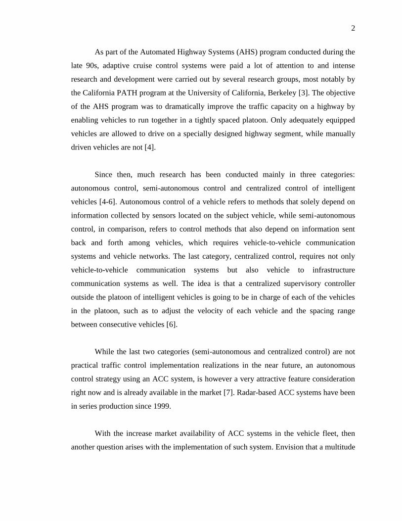
Imagine a vehicle running on an inclined road as shown in Figure 2.1 [11].
is the gravity of the vehicle, where is the vehicle mass and is the gravity
acceleration; is the incline angle of the road; is the height of the vehicle’s Center of
Gravity(CG); and are torques applied to the front and rear wheels; and
are longitudinal forces on the vehicle at the front and rear wheel ground contact points,
respectively; and are vertical load forces on the vehicle at the front and rear
ground contact points, respectively; is the longitudinal vehicle velocity and
is the
6
longitudinal acceleration of the vehicle, where and are the distances between CG and
the front and rear axles, respectively.
Figure 2.1 Vehicle Dynamics and Motion
The external longitudinal forces acting on the vehicle include longitudinal tire
forces, gravitational forces, aerodynamic drag forces and rolling resistance forces. The
vehicle motion is determined by the net effect of all these external forces and torques
applied on it. The following equations describe all the relationships among these external
forces [11, 12].
( )
( )
( ) ( )
where is the air drag coefficient, A is the frontal area and is the air density.
From vertical perspective, zero vertical acceleration and zero pitch torque require
( )
( )

7
( )
( )
where
( )
2.2. Engine Model
If the intake manifold filling dynamics are ignored, a first order engine model can
be used to represent engine dynamics. It’s still valid to use such engine model for some
longitudinal vehicle control applications if the bandwidth of the control system to be
designed is low [13].
In the case where a first order model is used for simulation, the engine dynamics
consist of just one state , the rotational velocity of an engine and is given by
( )
where is the engine inertia, is the load torque and ( ) is the net torque
after losses, and can be obtained from an engine map. ( ) is provided as a steady
state function of the engine rotational velocity and the throttle angle as inputs.
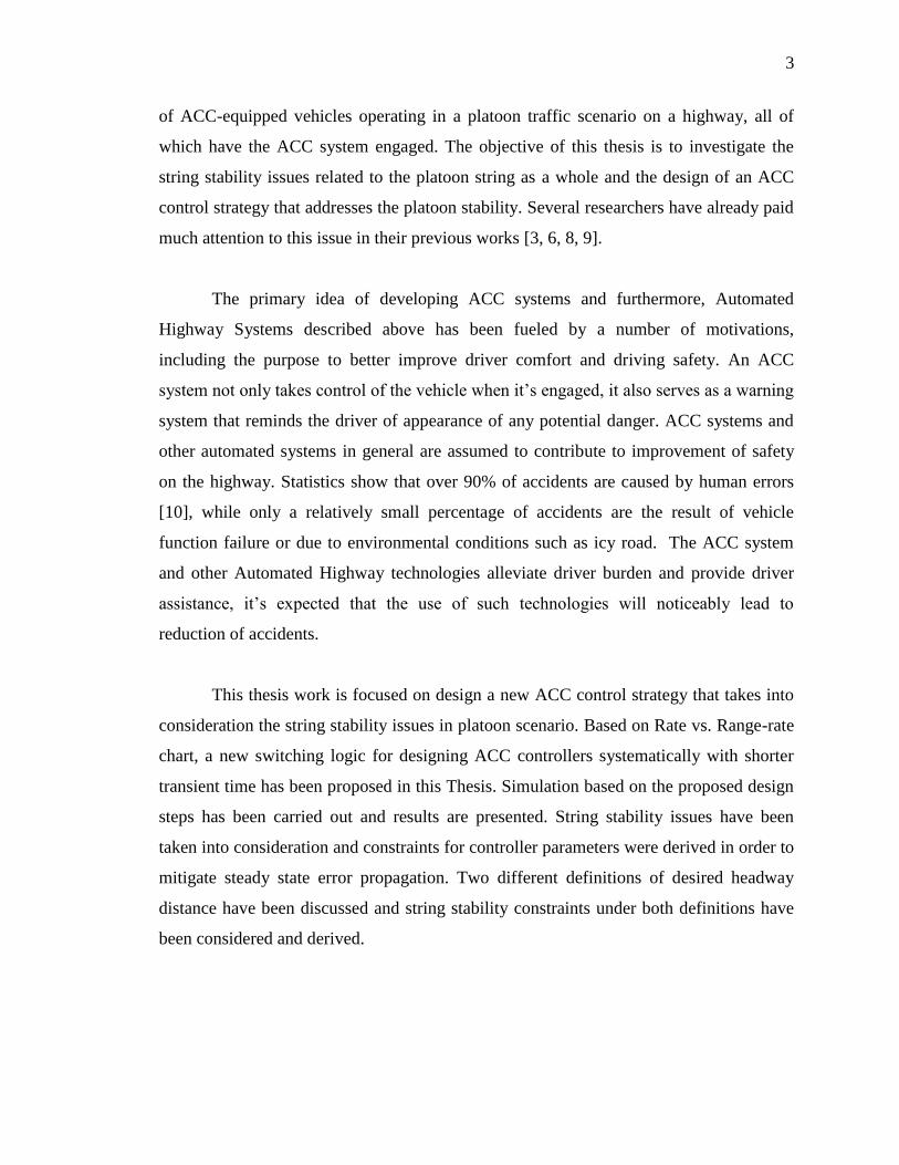
Figure 2.2 represents a typical engine map with engine rotational velocity and
the throttle angle as inputs, the net torque after losses ( ) as output [12]. It’s
clear that ( ) increases with throttle angle nonlinearly but monotonically. For
each throttle, ( ) initially increases with rotational engine velocity , reaches a
maximum and then decreases.
8
Figure 2.2 First Order Engine Map
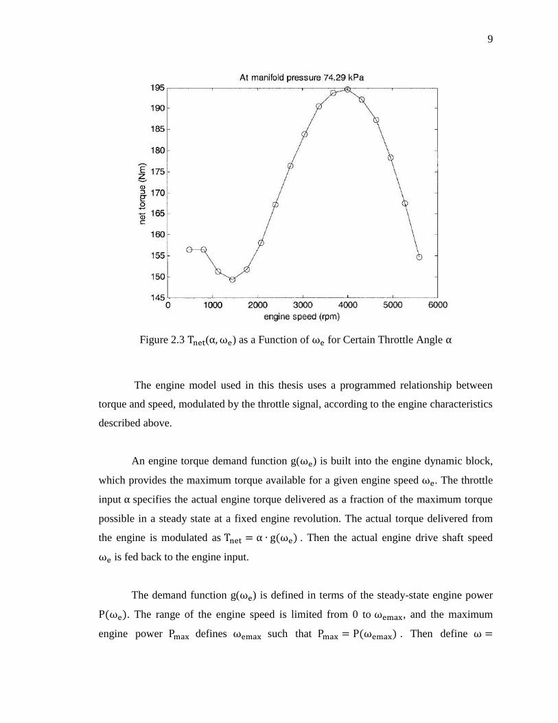
Thus for each throttle angle, there is an engine speed at which maximum
torque is achieved, because throttle angle relates to the pressure in the intake manifold
of an engine, as seen in Figure 2.3.
9
Figure 2.3 ( ) as a Function of for Certain Throttle Angle
The engine model used in this thesis uses a programmed relationship between
torque and speed, modulated by the throttle signal, according to the engine characteristics
described above.
An engine torque demand function g( ) is built into the engine dynamic block,
which provides the maximum torque available for a given engine speed . The throttle
input specifies the actual engine torque delivered as a fraction of the maximum torque
possible in a steady state at a fixed engine revolution. The actual torque delivered from
the engine is modulated as ( ) . Then the actual engine drive shaft speed
is fed back to the engine input.
The demand function g( ) is defined in terms of the steady-state engine power
( ). The range of the engine speed is limited from 0 to , and the maximum
engine power defines such that ( ) . Then define
10
and ( ) ( ). Since power is the product of torque and angular
velocity, the torque demand function is thus
( ) (
) [ ( )
] ( )
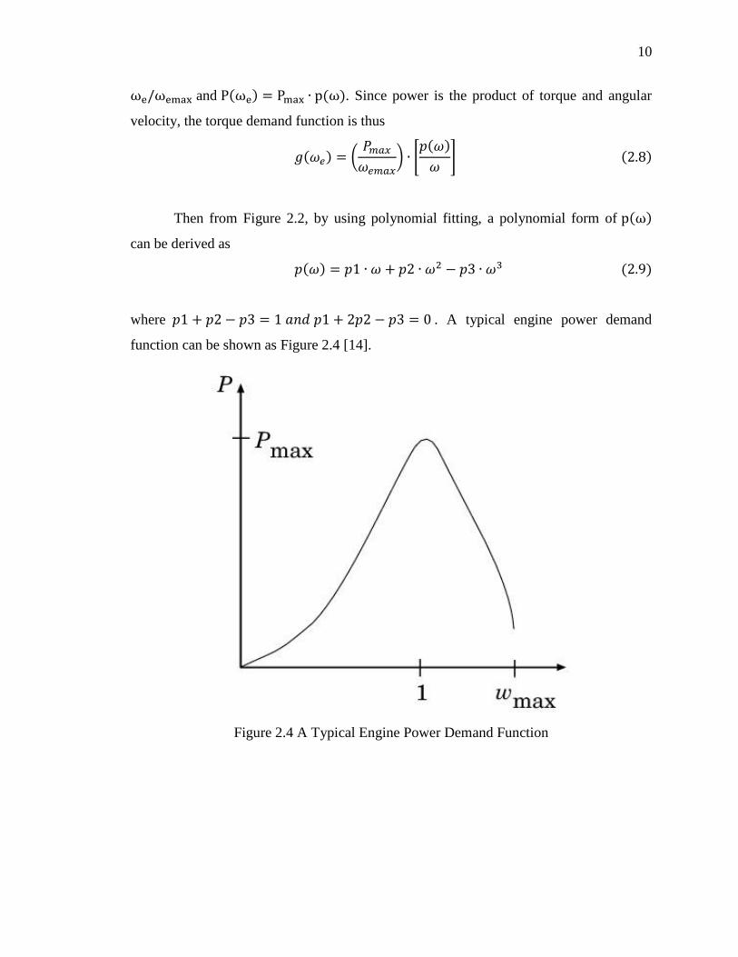
Then from Figure 2.2, by using polynomial fitting, a polynomial form of ( )
can be derived as
( ) ( )
where . A typical engine power demand
function can be shown as Figure 2.4 [14].
Figure 2.4 A Typical Engine Power Demand Function

11
2.3. Drivetrain Dynamic
Through powertrain dynamic the power generated by engine flows from the
engine to the wheels, and load flows backwards from wheels to the engine shaft [15],
shown as in Figure 2.5.
Figure 2.5 Power and Load Flow in a Vehicle Drivetrain
2.3.1. Torque Converter
Torque converter is the equipment that couples torque from engine side to the
transmission side and couples load backwards. It consists of two major components, a
pump on the engine side and a turbine on the transmission side. The fins of the pump are
attached to the flywheel of the engine and therefore turn at the same speed as the engine.
The turbine is connected to the transmission and causes the transmission to spin at the
same speed as the turbine, and then basically this mechanism moves the wheels after
torque is passed through the gear box of the transmission [12].
Torque converter has three operational modes, stall mode, acceleration mode and
coupling mode. During stall mode when the engine shaft is transferring power to the
pump but the turbine cannot rotate due to constant braking, the torque converter can
produce maximum torque multiplication (called stall ratio in this case) if sufficient input
power is applied. When the load is accelerating but there still is a relatively large
difference between pump and turbine speed, the torque converter works in acceleration
mode. In this case, the amount of multiplication will depend upon the actual difference
speed of the pump and the turbine.
12
The coupling mode of the torque converter is the main working mode. In this
mode, the turbine has reached over 90% of the speed of the pump. Torque multiplication
has basically ceased and the torque converter is working as a plain fluid coupling.
Usually in this mode, a lock-up clutch is applied to improve fuel efficiency.
In the simulation model on which this thesis is based, an assumption is made such
that the torque converter is always working in the coupling mode and the loss caused by
the torque converter is neglected.
2.3.2. Transmission Model
Transmission, a.k.a. gearbox, provides speed and torque from the engine through
connection with the turbine in torque converter. Often, a transmission will have multiple
gear ratios, with the ability to switch between them as speed varies [16].
In the simulation used by this thesis, two differential blocks are used to represent
differential gear that couples rotational motion about the longitudinal axis to rotational
motion of the tow lateral axes. In terms of the driving gear ratio , the longitudinal
motion is related to the sum of the lateral motions,
( ) ( )
where and are the speeds of the front wheels and the sum of the motion is the
transformed longitudinal motion, as long as the longitudinal axis is connected.
The torques along the lateral axes, and are constrained to the longitudinal
torque input, in a superposition way,
( )
Combining Equation 2.10 and Equation 2.11, we have
( )
( )
13
where is the transmission gear ratio. Equation 2.12 is the transmission model used in
the simulation [17].
2.3.3. Wheel Model
The tire is a flexible body what contacts the road surface and gives the subject on
it the force needed to move forward or backward. When a torque is applied to the wheel
axle, the tire deforms, pushes the ground and delivers a reverse force back from the
ground to the wheel, and then pushes the wheel forward or backward.
Longitudinal forces and in Equation 2.4 and Equation 2.5 are friction
forces from the ground that act on the tires, which depend on three factors, the slip ratio,
the normal load on each tire and the friction coefficient of the tire-road interface [18].
A longitudinal slip of a tire is defined as the difference between the actual
longitudinal velocity at the axle of the wheel, in Figure 2.1, and the equivalent
rotational velocity of the tire, where is the effective tire radius and is the
rotational speed of the wheel. In other words, longitudinal slip is equal to .
Longitudinal slip ratio is defined differently during different situations.
During braking:
( )
During acceleration:
( )

14
From experimental data, Figure 2.6 shows why and how slip ratio affects
longitudinal tire forces. It is clear that in the case where longitudinal slip is small, the
longitudinal tire force is approximately proportional to the slip ratio [18].
Figure 2.6 Longitudinal Tire Force as a Function of Slip Ratio
A Simulink tire block simulates a tire as a rigid-wheel, flexible-body combination
in contact with the road, including only longitudinal motion. Figure 2.7 shows the
dynamics and motion of a tire model used in the Simulink library, which is for a driving
wheel. Figure 2.8 shows different situation when the wheel is a following wheel.
15
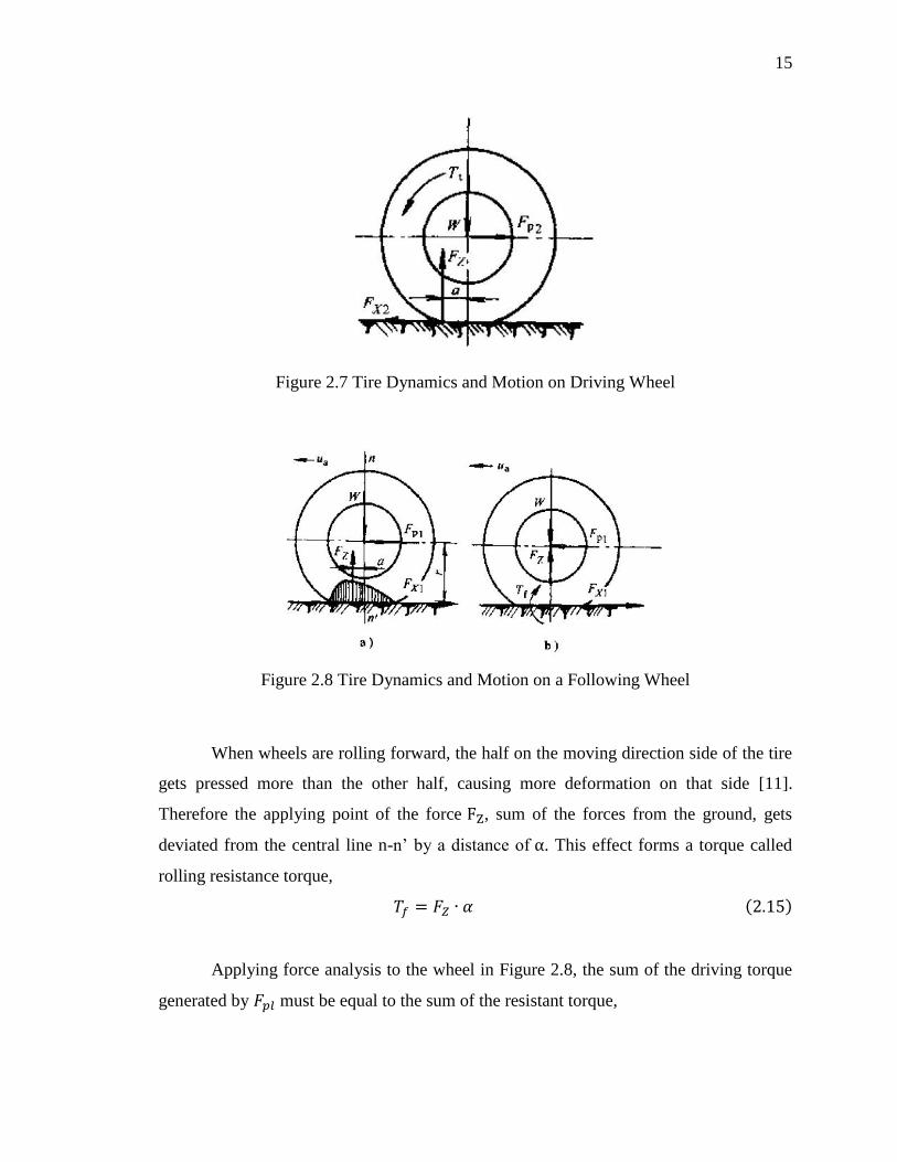
Figure 2.7 Tire Dynamics and Motion on Driving Wheel
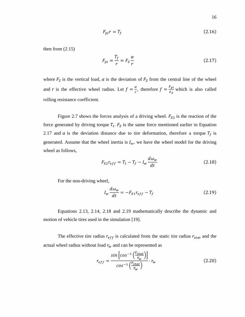
Figure 2.8 Tire Dynamics and Motion on a Following Wheel
When wheels are rolling forward, the half on the moving direction side of the tire
gets pressed more than the other half, causing more deformation on that side [11].
Therefore the applying point of the force , sum of the forces from the ground, gets
deviated from the central line n-n’ by a distance of . This effect forms a torque called
rolling resistance torque,
( )
Applying force analysis to the wheel in Figure 2.8, the sum of the driving torque
generated by must be equal to the sum of the resistant torque,
16
( )
then from (2.15)
( )
where is the vertical load, is the deviation of from the central line of the wheel
and is the effective wheel radius. Let
, therefore
which is also called
rolling resistance coefficient.
Figure 2.7 shows the forces analysis of a driving wheel. is the reaction of the
force generated by driving torque . is the same force mentioned earlier in Equation
2.17 and is the deviation distance due to tire deformation, therefore a torque is
generated. Assume that the wheel inertia is , we have the wheel model for the driving
wheel as follows,
( )
For the non-driving wheel,
( )
Equations 2.13, 2.14, 2.18 and 2.19 mathematically describe the dynamic and
motion of vehicle tires used in the simulation [19].
The effective tire radius is calculated from the static tire radius and the
actual wheel radius without load and can be represented as
* (
)+
( )
( )
17
Now the following relationship is shown as . The total
longitudinal force is given by
( )
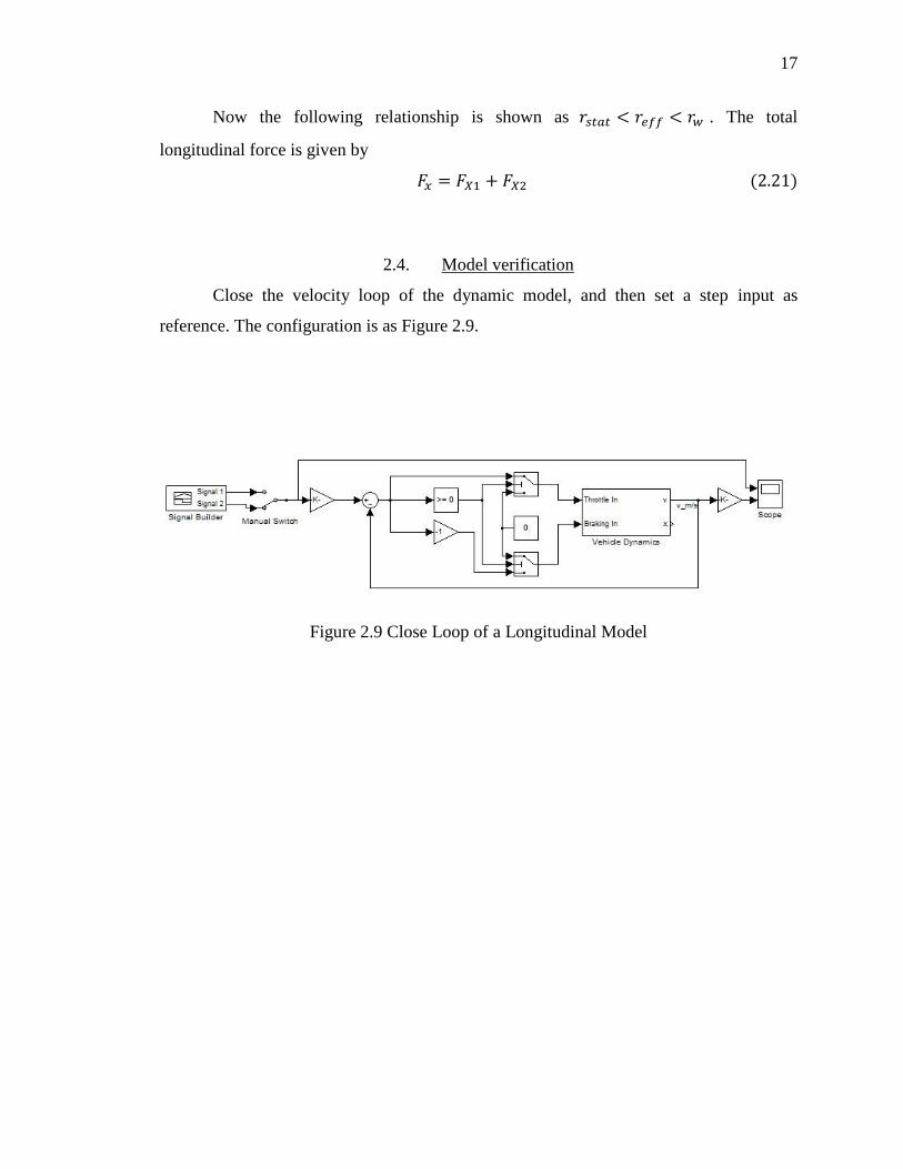
2.4. Model verification
Close the velocity loop of the dynamic model, and then set a step input as
reference. The configuration is as Figure 2.9.
Figure 2.9 Close Loop of a Longitudinal Model
18
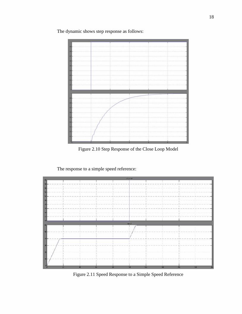
The dynamic shows step response as follows:
Figure 2.10 Step Response of the Close Loop Model
The response to a simple speed reference:
Figure 2.11 Speed Response to a Simple Speed Reference
19
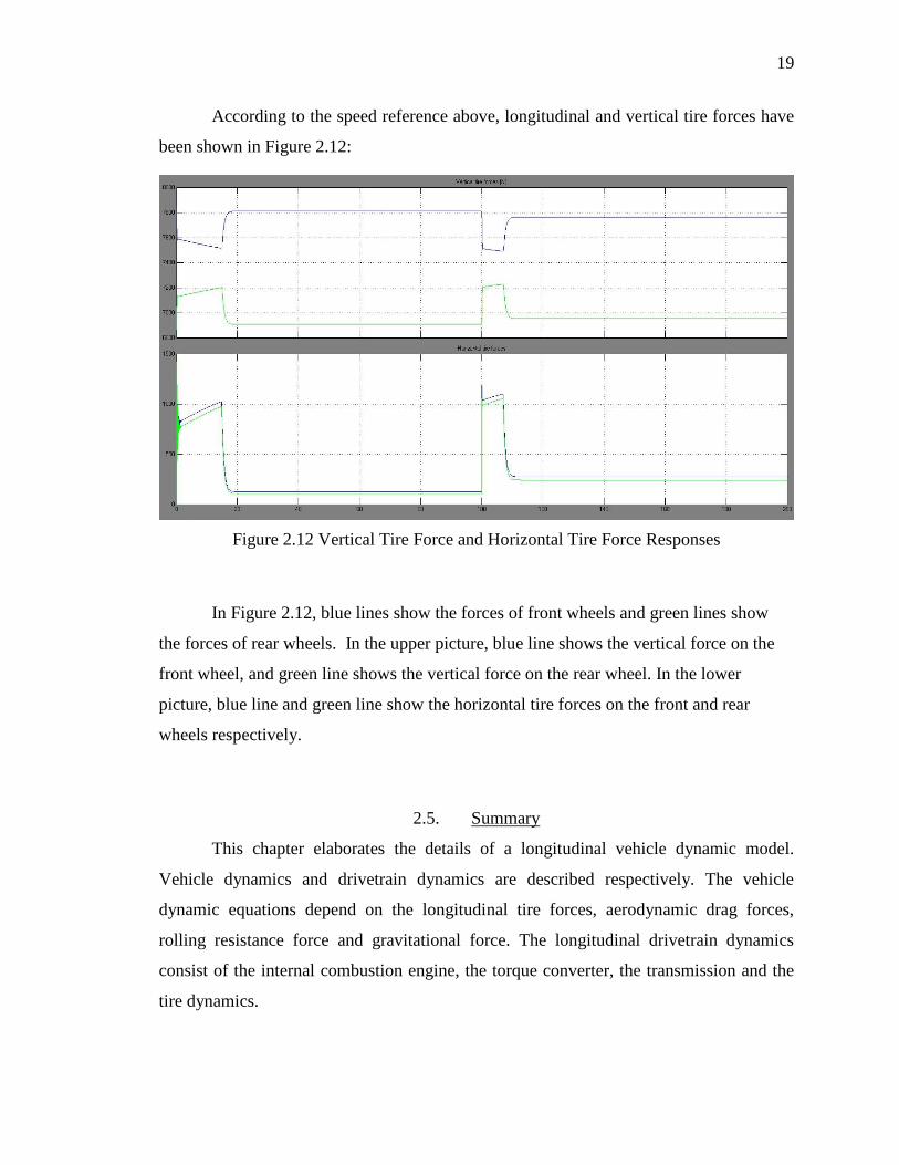
According to the speed reference above, longitudinal and vertical tire forces have
been shown in Figure 2.12:
Figure 2.12 Vertical Tire Force and Horizontal Tire Force Responses
In Figure 2.12, blue lines show the forces of front wheels and green lines show
the forces of rear wheels. In the upper picture, blue line shows the vertical force on the
front wheel, and green line shows the vertical force on the rear wheel. In the lower
picture, blue line and green line show the horizontal tire forces on the front and rear
wheels respectively.
2.5. Summary
This chapter elaborates the details of a longitudinal vehicle dynamic model.
Vehicle dynamics and drivetrain dynamics are described respectively. The vehicle
dynamic equations depend on the longitudinal tire forces, aerodynamic drag forces,
rolling resistance force and gravitational force. The longitudinal drivetrain dynamics
consist of the internal combustion engine, the torque converter, the transmission and the
tire dynamics.
20
3. ACC CONTROLLER DESIGN
3.1. Introduction
ACC (Adaptive Cruise Control) system is an extension of the standard cruise
control system that takes control of the vehicle speed and tries to maintain a pre-set
velocity by the driver. For ACC operation, radars or other type of detection sensors such
as a lidar are used to accomplish the function that consistently measures the distance to a
preceding in-lane vehicle. The sensor is integrated into the subject vehicle, shown in
Figure 3.1. The ACC controller processes the kinematic information of the preceding in-
lane vehicle to autonomously control the brake and throttle system to regulate the vehicle
speed.
When no preceding in-lane vehicle is detected or is sufficiently apart from the
subject vehicle, the ACC controller works the same way as a conventional cruise
controller does. Once a preceding vehicle is detected, the ACC controller determines
whether or not the subject vehicle can continue running safely at the current driver
selected set-speed. If a potential hazardous condition is assessed, such as when the
preceding vehicle is moving at a slower speed, or the distance between the subject
vehicle and the preceding vehicle is getting too close, the ACC controller will switch
from speed control mode to headway control mode. During headway control mode
operation, in order to maintain a desired headway for the subject vehicle, both throttle
and brake are used.

21
Figure 3.1 ACC System in Action
An important function of an ACC controller is to maintain a desired headway
distance between the subject vehicle and preceding in-lane vehicle to reduce potential
hazardous events from taking place. An ACC system also provides better driving
experience and comfort by allowing the system to take control of the vehicle, which is an
extension of the conventional cruise control system. Different from Automated Highway
System, the ACC system is an autonomous system that doesn’t depend on either wireless
vehicle-to-vehicle communication or communication between vehicle and infrastructure.
Besides the two operational modes, the ACC controller would also have to decide
the condition of when and where to switch between the two modes. Thus, a transitional
switching logic that decides which ACC control mode should be activated has to be
designed, according to different traffic situations.
This chapter will focus on the design of transitional switching logic; the next
chapter will focus on the string stability analysis of ACC controlled vehicles while
operating in a platoon traffic scenario.
3.2. Problem Description
Figure 3.2 shows the basic concepts based on which the ACC controller design
would be mathematically modeled. Two consecutive vehicles in a generic platoon traffic
situation are illustrated in the figure.

22
Figure 3.2 Variables Definitions for Design of an ACC Controller
: Velocity of the preceding vehicle.
: Relative position (based on a 1-D coordinate) of the preceding vehicle.
: Velocity of following vehicle (subject vehicle).
: Relative position of following vehicle (subject vehicle).
: Pre-set reference speed of the following vehicle by driver.
: Actual distance between two consecutive vehicles.
: Desired headway distance between the two vehicles.
: Switching range by which ACC controller switches between the two
modes.
: Braking range, in which the following vehicle has to apply maximum
braking to avoid potential collision.
: Buffer zone before reaching the equilibrium point.
I: Speed control zone.
II: Headway control zone.
III: Moderate Braking zone.
IV: Maximum Braking zone.
23
The headway control problem can be described as to develop a system that
maintains a desired headway distance , between two consecutive vehicles by
modulating the speed of the following vehicle, as shown in Figure 3.2.
Once the onboard sensor of the following vehicle detects the presence of a
preceding vehicle and the ACC system is engaged, the ACC control strategy starts to take
control of the vehicle.
When the following vehicle reaches Zone I in Figure 3.2, the system determines
there is still enough distance left from the preceding vehicle, then according to the driver
pre-set speed, the controller maintains the pre-set speed as a conventional cruise
controller. If the pre-set speed is greater than that of the preceding vehicle, the range
between the two vehicles is going to gradually shrink, that means, the following vehicle
is catching up with the preceding one.
After the following vehicle reaches Zone II, the ACC controller switches from
speed control mode to headway control mode. The line between Zone II and Zone III
indicates the desired distance.
There are basically two different strategies to control the velocity of the following
vehicle, based on different definitions of the desired headway distance . The
different definitions of will result in totally different results. The controller regulates
the speed of the following vehicle to catch up and then maintain the desired distance ,
depending on the preceding vehicle kinematic information available to the following
vehicle’s onboard controller as provided by the detection sensors.
In a cut-in case, if the following vehicle’s onboard ACC controller detects a cut-in
vehicle that causes the range is within Zone III, the ACC controller will switch to
headway control instantly and reduce the following vehicle’s speed, which enlarges the

24
range to be equal to . In extreme cases when the actual range is within Zone IV,
maximum braking would be applied to avoid a potential collision.
3.2.1. Constant Headway Distance Strategy
Constant headway distance strategy simply means that regardless of the velocity
of the preceding vehicle or that of the following vehicle, the desired headway distance
from the subject vehicle to the preceding vehicle to be a constant. Previous work has
shown that this control strategy is not suitable for autonomous control applications such
as ACC because it has been proven to be unstable in vehicle string scenario [8].
3.2.2. Constant Headway Time Strategy
A constant headway time strategy refers to a headway control condition that tries
to maintain a constant headway time “ ”. In this case, the desired headway distance
is not a constant but a linear function of either the velocity of preceding vehicle or that
the following vehicle [20]. Both situations will be discussed in this thesis.
The famous “Two Second Rule” is an example of this headway strategy. It’s a
rule by which a driver may maintain a safe following distance at any speed. The rule
states that a driver should stay at least two seconds behind any vehicle that is directly in
front of the driver’s vehicle. In this case, the two second is the constant headway time
mentioned above.
For drivers, the “two second” headway time rule inherently includes human
response time. However, with the incorporation of an onboard controller system, the
response time is much shorter than that of the human’s. As such, in many ACC system
implementations, multiple timed-headway gap settings are offered to the driver, typically
ranging from 1 second to 2.2 seconds. The driver is allowed to select the appropriate
headway setting based upon personal preferences and traffic density.

25
3.3. Range Vs. Range-rate Chart
A Range (R) versus Range-rate (dR/dt or Rdot) chart can be used to describe the
control mode switching logic problem more efficiently and effectively [21]. Relative
position and relative velocity between the two consecutive vehicles can be represented in
such chart. Define variables as follows,
At the steady state equilibrium point, the range would be equal to the desired
headway distance and the velocity of the following vehicle would be equal to the
velocity of the preceding vehicle .
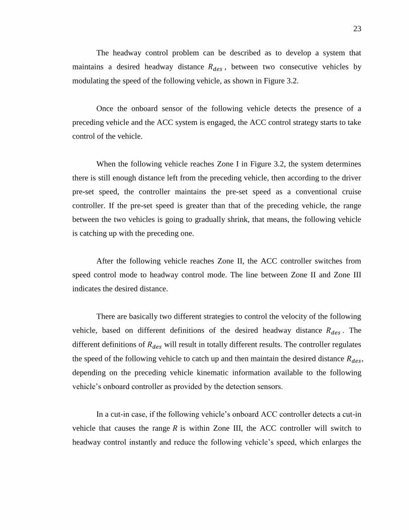
3.3.1. Properties of the Range Vs. Range-rate Chart
Certain properties need to be elaborated before any mathematical formulation is
developed on the R-Rdot chart. Figure 3.3 shows a basic principle concerning the
direction of trajectories as time increases.
In the upper left quadrant, because , that means and the
following vehicle is moving faster than the preceding vehicle. In this situation, the
trajectories on the R-Rdot chart have the tendency to go downward since the value R
tends to decrease.
In the upper right quadrant, because , that means and the
following vehicle is moving slower than the preceding vehicle. In this situation, the
trajectories on the R-Rdot chart have the tendency to go upward since the value R tends to
increase.
Possible equilibrium point on the R-Rdot chart should be on the vertical axis,
where and .
26
Figure 3.3 Properties of R-Rdot Chart
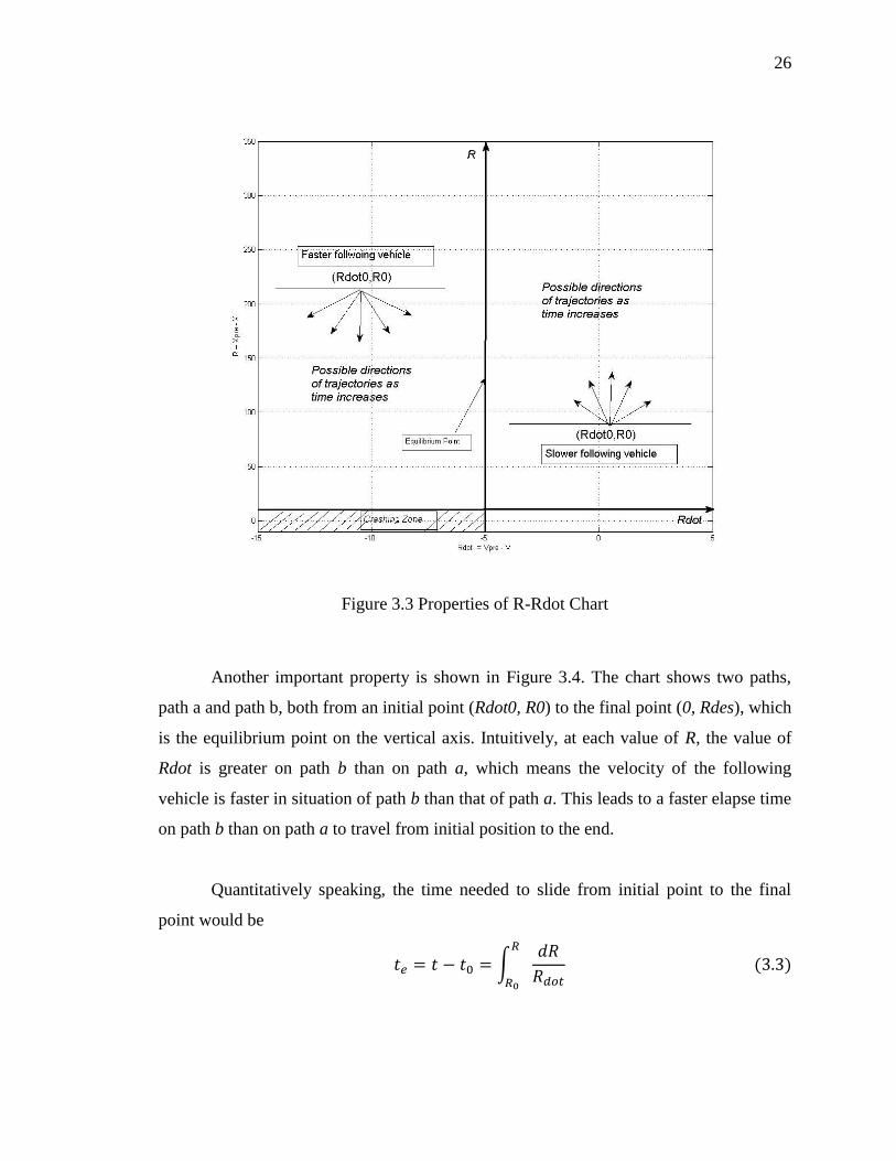
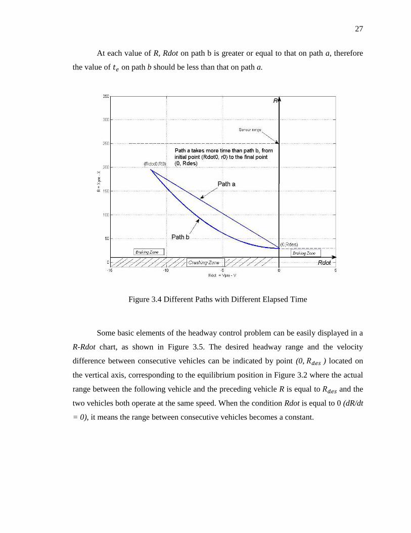
Another important property is shown in Figure 3.4. The chart shows two paths,
path a and path b, both from an initial point (Rdot0, R0) to the final point (0, Rdes), which
is the equilibrium point on the vertical axis. Intuitively, at each value of R, the value of
Rdot is greater on path b than on path a, which means the velocity of the following
vehicle is faster in situation of path b than that of path a. This leads to a faster elapse time
on path b than on path a to travel from initial position to the end.
Quantitatively speaking, the time needed to slide from initial point to the final
point would be
∫
27
At each value of R, Rdot on path b is greater or equal to that on path a, therefore
the value of on path b should be less than that on path a.
Figure 3.4 Different Paths with Different Elapsed Time
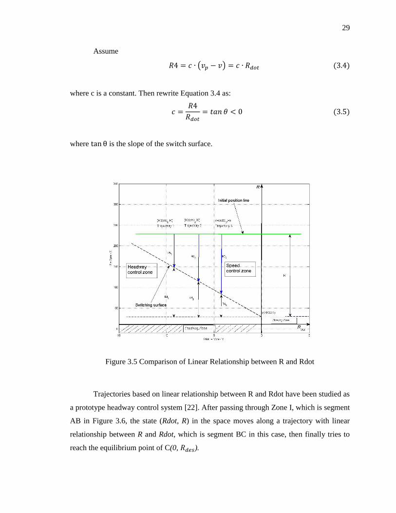
Some basic elements of the headway control problem can be easily displayed in a
R-Rdot chart, as shown in Figure 3.5. The desired headway range and the velocity
difference between consecutive vehicles can be indicated by point (0, ) located on
the vertical axis, corresponding to the equilibrium position in Figure 3.2 where the actual
range between the following vehicle and the preceding vehicle R is equal to and the
two vehicles both operate at the same speed. When the condition Rdot is equal to 0 (dR/dt
= 0), it means the range between consecutive vehicles becomes a constant.

28
3.3.2. A Linear Relationship between R and Rdot
The zones (Zone I, Zone II, Zone III, and Zone IV) and ACC control modes
(speed control & headway control) represented in Figure 3.2 can be correspondly mapped
to the R-Rdot chart of Figure 3.3. Furthermore, the boundaries of each zone indicate the
switching surface that different control strategy is needed to achieve corresponding
control goal. Quantitative descriptions are going to be explained in this section to gain a
better understanding of the chart. A whole set of switching strategies for design of ACC
controller will be represented using this chart later.
First of all, a comparison between Figure 3.2 and Figure 3.7 is necessary. Figure
3-2 shows the image of R-Rdot linear relationship in an intuitive way whereas Figure 3.7
shows the relationship in an R-Rdot chart. Since the distance R4 in Figure 3.6 serves as a
buffer before the equilibrium position, then Zone II is called the buffer zone. By
definition, . While operating in Zone I (R5), the following vehicle
keeps running at the pre-set speed . Once the following vehicle proceeds into Zone II,
control strategy switches from speed control mode to headway control mode and
continues to approach the equilibrium point .
The above situation can be represented by one of the three trajectories in Figure
3.7. Take trajectory 1 for example. The initial position in the space is located on the
“Initial Position Line” shown in the chart. Then as the following vehicle keeps
approaching the preceding vehicle at the driver’s pre-set speed over R5, the state position
goes downward vertically along the trajectory in the chart, until it reaches the switching
surface. After passing the switching surface, the following vehicle switches from speed
control mode to headway control mode. Trajectory 2 and trajectory 3 are both similar
processes with different initial position and different values of R5 and R4.
Since only two vehicles are considered in this case, we can redefine and
.
29
Assume
( )
where c is a constant. Then rewrite Equation 3.4 as:
where is the slope of the switch surface.
Figure 3.5 Comparison of Linear Relationship between R and Rdot
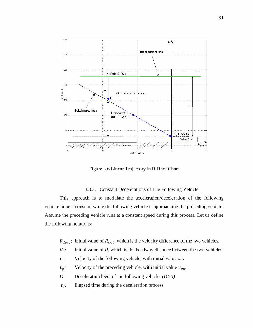
Trajectories based on linear relationship between R and Rdot have been studied as
a prototype headway control system [22]. After passing through Zone I, which is segment
AB in Figure 3.6, the state (Rdot, R) in the space moves along a trajectory with linear
relationship between R and Rdot, which is segment BC in this case, then finally tries to
reach the equilibrium point of C(0, ).

30
The equation of the trajectory BC is as follows:
where -c is the slope of the segment BC in Figure 3.6. Obviously c should be greater than
0 here, and is different from Equation 3.5 because of the additional minus sign in
Equation 3.6.
Rewriting Equation 3.6 as a general first order differential equation with the
initial condition , we have the following equation:
Solving Equation 3.7 with the initial condition, one obtains
⁄ (
⁄ )
where c is like a time constant that decides how fast the system would approach the
equilibrium point. However from the solution, it is clear that no matter how long it takes,
the system would only approach the final position but would never reach it because of the
exponential term in Equation 3.8. However, from a practical consideration, at
time, the system will get close enough to the equilibrium point, with over 99% of the
whole length of segment BC.
31
Figure 3.6 Linear Trajectory in R-Rdot Chart
3.3.3. Constant Decelerations of The Following Vehicle
This approach is to modulate the acceleration/deceleration of the following
vehicle to be a constant while the following vehicle is approaching the preceding vehicle.
Assume the preceding vehicle runs at a constant speed during this process. Let us define
the following notations:
: Initial value of , which is the velocity difference of the two vehicles.
: Initial value of R, which is the headway distance between the two vehicles.
: Velocity of the following vehicle, with initial value .
: Velocity of the preceding vehicle, with initial value .
D: Deceleration level of the following vehicle. (D>0)
: Elapsed time during the deceleration process.
32
From the definitions and assumptions above,
From equations 3.1, 3.2, 3.9 and 3.10,
where is the initial value of on the trajectory.
From Equation 3.11
which is the estimated amount of time needed for the following vehicle to reach the
equilibrium point. In the R-Rdot chart, it also represents the time needed for the states to
move from the initial point to the end of the trajectory, where and .
Therefore, if let in Equation 3.12,
Equation 3.13 shows the time elapsed (for Rdot<0) in reaching the vertical axis,
i.e., Rdot=0.
Rewriting Equation 3.11 as,
⇔
⇔
then integrating the two sides of Equation 3.14 with respect to time,

33
∫
∫
∫
Substituting in Equation 3.15 with Equation 3.12 and rearranging the two sides,
we obtain
When the following vehicle reaches equilibrium point, , R is expected to
be , which means Equation 3.16 should be equal to ,
Therefore a relationship between R and Rdot has been derived and shown in
Figure 3.7. Depending on how large the value of deceleration would be, the elapsed time
of the deceleration process can be calculated by Equation 3.13. When a larger
deceleration level is selected, the trajectory of the deceleration process is shifting toward
the more negative side of Rdot, which is shown in Figure 3.8.

34
Figure 3.7 Trajectory of Constant Deceleration Strategy

35
Figure 3.8 Trajectories with Different Deceleration Level
3.4. Design of A Headway Control Strategy
Assumptions had been made that a reliable conventional cruise control system
had already been available to represent the speed control mode and the simulation has
been conducted in a situation in which the preceding vehicle is moving at a constant
speed for most of the time. A desirable comparison can only be made when the desired
headway distance, i.e., is fixed in the R-Rdot chart.
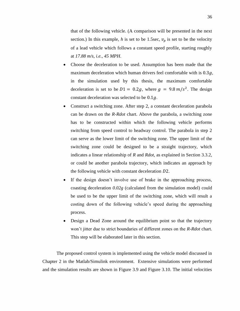
With reference to Figure 3.9 below, the design process proposed in this thesis
consists of the following steps:
Define the desired headway distance for a selected velocity and headway
time. For example, define , where h is called headway time
with second as its unit and is the velocity of the preceding vehicle.
Usually is a function of either the velocity of the preceding vehicle or
36
that of the following vehicle. (A comparison will be presented in the next
section.) In this example, h is set to be 1.5sec, is set to be the velocity
of a lead vehicle which follows a constant speed profile, starting roughly
at 17.88 m/s, i.e., 45 MPH.
Choose the deceleration to be used. Assumption has been made that the
maximum deceleration which human drivers feel comfortable with is ,
in the simulation used by this thesis, the maximum comfortable
deceleration is set to be , where . The design
constant deceleration was selected to be .
Construct a switching zone. After step 2, a constant deceleration parabola
can be drawn on the R-Rdot chart. Above the parabola, a switching zone
has to be constructed within which the following vehicle performs
switching from speed control to headway control. The parabola in step 2
can serve as the lower limit of the switching zone. The upper limit of the
switching zone could be designed to be a straight trajectory, which
indicates a linear relationship of R and Rdot, as explained in Section 3.3.2,
or could be another parabola trajectory, which indicates an approach by
the following vehicle with constant deceleration .
If the design doesn’t involve use of brake in the approaching process,
coasting deceleration 0.02g (calculated from the simulation model) could
be used to be the upper limit of the switching zone, which will result a
costing down of the following vehicle’s speed during the approaching
process.
Design a Dead Zone around the equilibrium point so that the trajectory
won’t jitter due to strict boundaries of different zones on the R-Rdot chart.
This step will be elaborated later in this section.
The proposed control system is implemented using the vehicle model discussed in
Chapter 2 in the Matlab/Simulink environment. Extensive simulations were performed
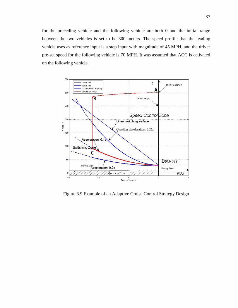
and the simulation results are shown in Figure 3.9 and Figure 3.10. The initial velocities
37
for the preceding vehicle and the following vehicle are both 0 and the initial range
between the two vehicles is set to be 300 meters. The speed profile that the leading
vehicle uses as reference input is a step input with magnitude of 45 MPH, and the driver
pre-set speed for the following vehicle is 70 MPH. It was assumed that ACC is activated
on the following vehicle.
Figure 3.9 Example of an Adaptive Cruise Control Strategy Design
38
Figure 3.10 Rdot and Spacing Error during the Simulation
39
From Figure 3.9, it’s clear that the range in between is getting shorter as time
epalses. Then after a while, when the trajectory on R-Rdot chart crosses the switching line
and gets into the switching zone, the ACC controller immediately switches from speed
control mode to headway control mode and starts to decelerate with a constant
deceleration of 0.1g, as designed in the example. In Figure 3.10, it shows the spacing
error between the actual spacing and the desired spacing becomes smaller and smaller as
time elapses and goes to zero eventually. Point A, B, C and D shown in Figure 3.10 are
corresponding to points with the same name in Figure 3.9.
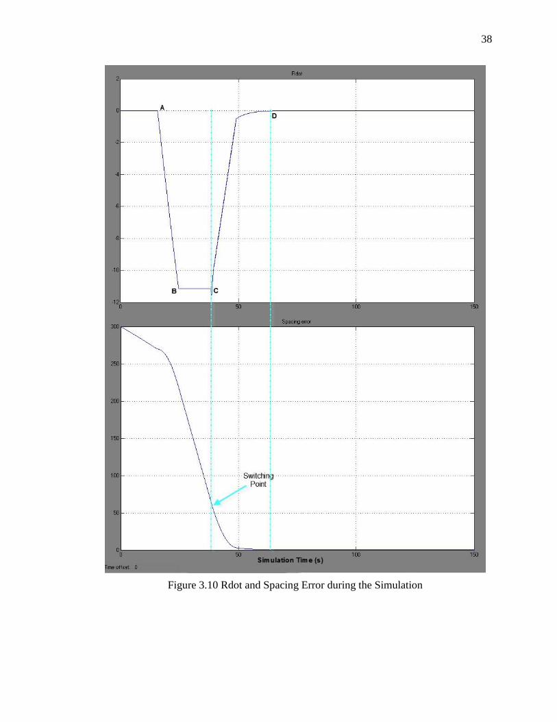
Another simulation case has been designed so that the preceding vehicle conducts
a sudden braking during headway control mode of the following vehicle, as shown in
Figure 3.11 and Figure 3.12, where y axis shows velocity input and x axis shows
simulation time in seconds.
Figure 3.11 Car Following Model
40
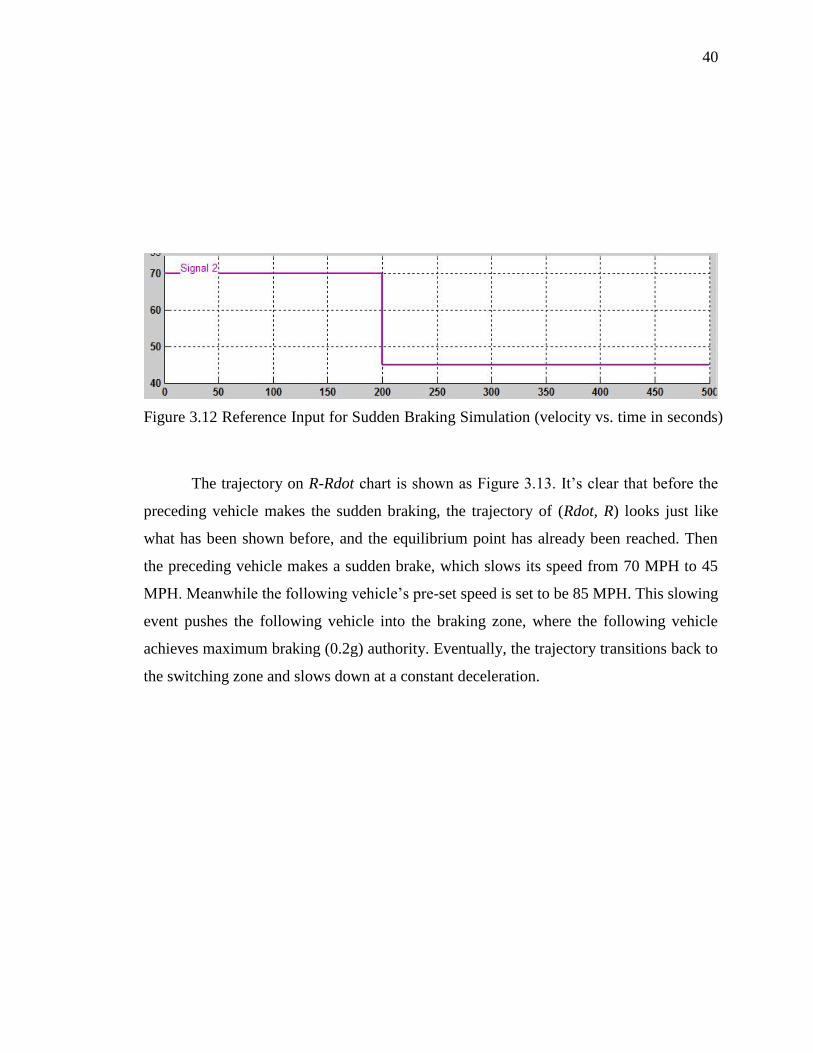
Figure 3.12 Reference Input for Sudden Braking Simulation (velocity vs. time in seconds)
The trajectory on R-Rdot chart is shown as Figure 3.13. It’s clear that before the
preceding vehicle makes the sudden braking, the trajectory of (Rdot, R) looks just like
what has been shown before, and the equilibrium point has already been reached. Then
the preceding vehicle makes a sudden brake, which slows its speed from 70 MPH to 45
MPH. Meanwhile the following vehicle’s pre-set speed is set to be 85 MPH. This slowing
event pushes the following vehicle into the braking zone, where the following vehicle
achieves maximum braking (0.2g) authority. Eventually, the trajectory transitions back to
the switching zone and slows down at a constant deceleration.

41
Figure 3.13 Trajectory with Sudden Braking of the Preceding Vehicle
In step 5 of the design procedures for the proposed ACC controller, a dead zone
should be designed around the equilibrium point (0, ) on the R-Rdot chart. The
reason for design a dead zone is because if a strict boundary is defined on the R-Rdot
chart between two separate zones with two control strategies leading to conflicting
control goals, the trajectory would be pushed back and forth within a small range on the
boundary. Although from a large scale, the jittering phenomenon is hardly noticeable,
it’ll still become an unstable issue for the whole system when the string of ACC
controlled vehicles gets longer.
42
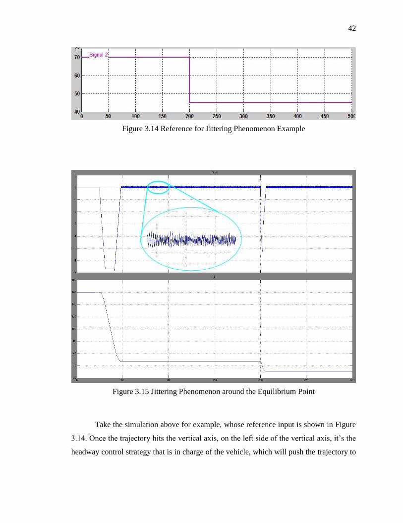
Figure 3.14 Reference for Jittering Phenomenon Example
Figure 3.15 Jittering Phenomenon around the Equilibrium Point
Take the simulation above for example, whose reference input is shown in Figure
3.14. Once the trajectory hits the vertical axis, on the left side of the vertical axis, it’s the
headway control strategy that is in charge of the vehicle, which will push the trajectory to
43
the vertical axis as close as possible; however since a PD controller is used to mitigate the
spacing error between the actual range of consecutive vehicles and the desired headway
distance, an overshoot is always possible. Due to the overshoot of the trajectory, it could
sometimes go across the vertical axis and get into the right side, within which the speed
control strategy will take charge. The speed control strategy forces the vehicle speed to
match the driver’s pre-set speed, which is greater than the speed of the preceding vehicle
because the trajectory initially comes from the left side where .
Therefore, the trajectory has to be pushed back to the left side of the vertical axis. After
that it will repeat the process described above another round and continue within a
relatively small range. It’s very clear when a close-up view is taken at the Rdot value as
time passes, separately, which is shown in Figure 3.15.
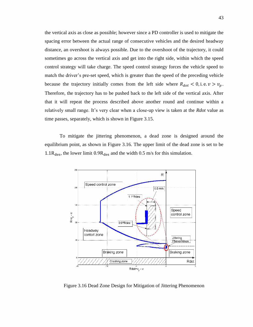
To mitigate the jittering phenomenon, a dead zone is designed around the
equilibrium point, as shown in Figure 3.16. The upper limit of the dead zone is set to be
, the lower limit and the width 0.5 m/s for this simulation.
Figure 3.16 Dead Zone Design for Mitigation of Jittering Phenomenon

44
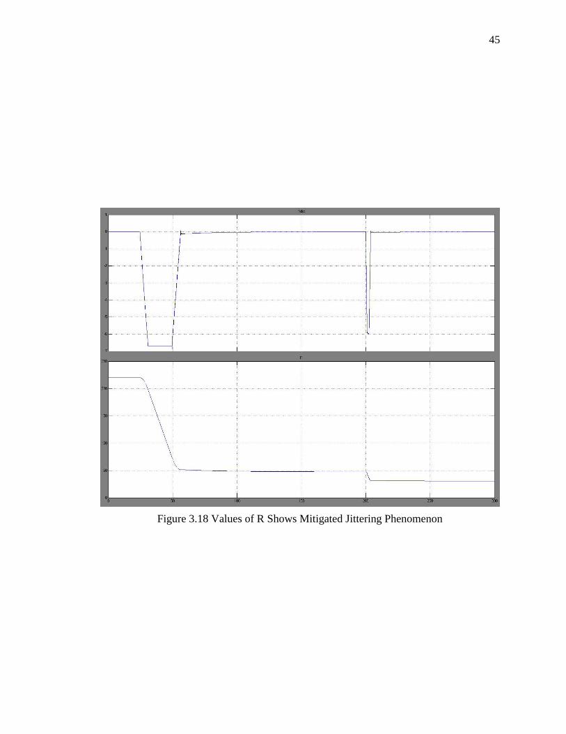
Within this dead zone headway control strategy applies, and speed control
strategy takes over beyond it. As a result of this modification, the result became quite
satisfactory, which is shown in Figure 3.17 and Figure 3.18.
Figure 3.17 R-Rdot Chart Showing No Jittering Phenomenon after Design of Dead Zone
45
Figure 3.18 Values of R Shows Mitigated Jittering Phenomenon
46
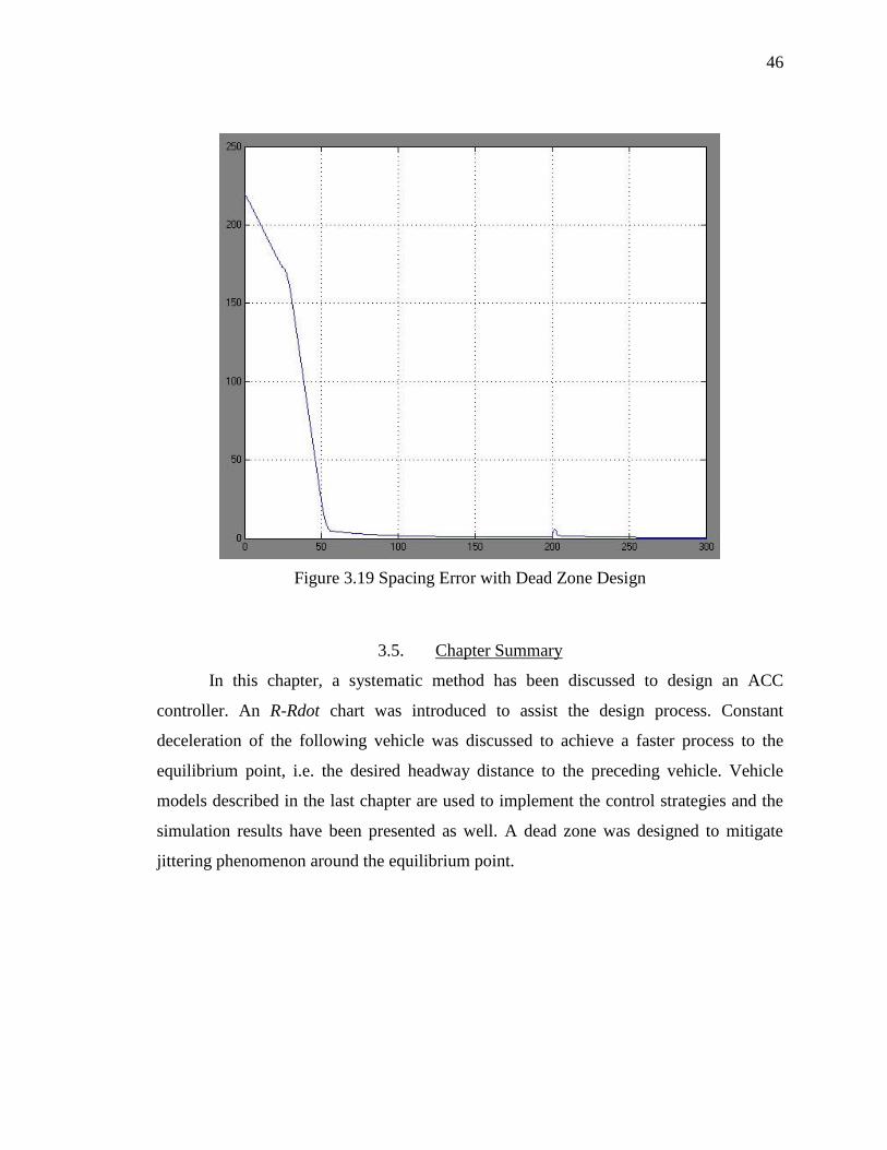
Figure 3.19 Spacing Error with Dead Zone Design
3.5. Chapter Summary
In this chapter, a systematic method has been discussed to design an ACC
controller. An R-Rdot chart was introduced to assist the design process. Constant
deceleration of the following vehicle was discussed to achieve a faster process to the
equilibrium point, i.e. the desired headway distance to the preceding vehicle. Vehicle
models described in the last chapter are used to implement the control strategies and the
simulation results have been presented as well. A dead zone was designed to mitigate
jittering phenomenon around the equilibrium point.
47
4. STRING STABILITY ANALYSIS
String stability issue has been addressed by other researchers after the adaptive
cruise control (ACC) concept was introduced [3]. The main problem is when many ACC
equipped vehicles form a vehicle platoon end to end, how the control algorithm is
designed to ensure that the spacing error, which is the deviation of the actual range from
the desired headway distance, would not amplify as the number of following vehicles
increases downstream along the platoon.
Different spacing policies have been briefly discussed in Section 3.2, including
constant spacing policy and constant headway time policy. In this chapter, these control
strategies will be discussed in detail.
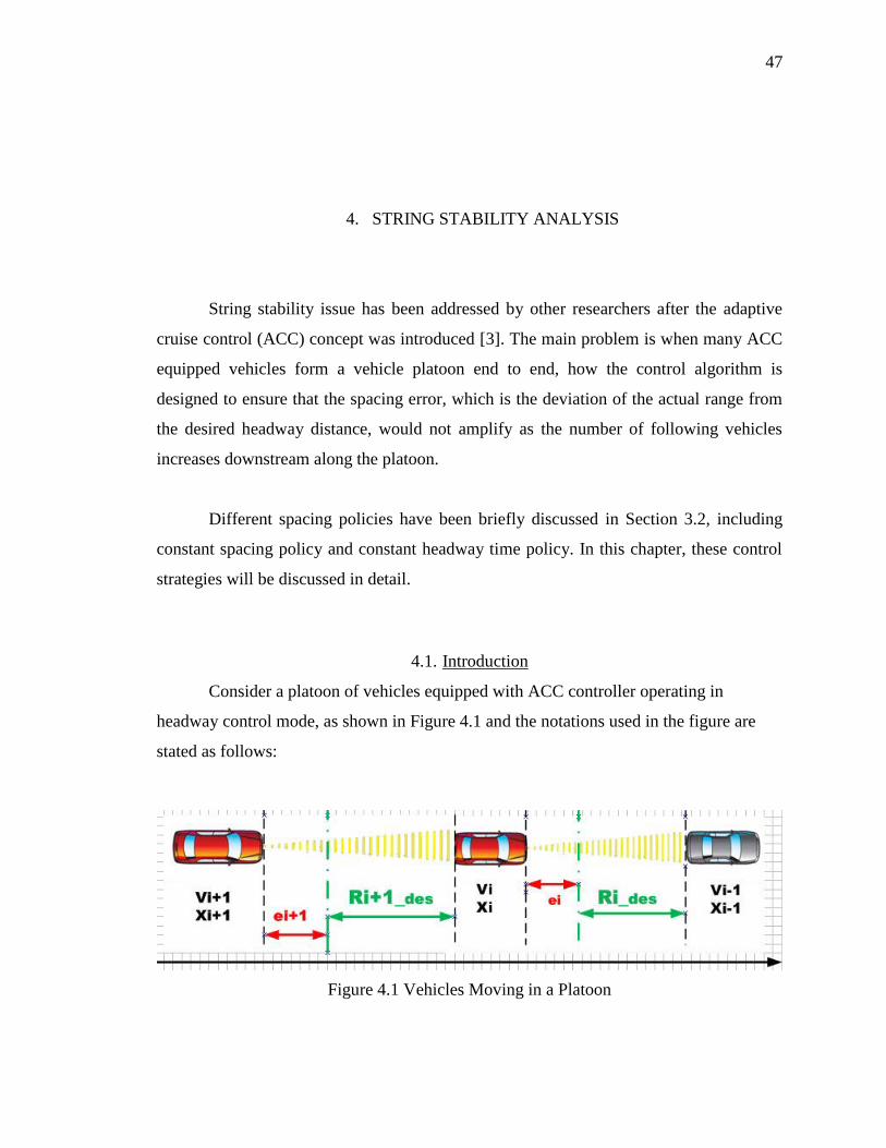
4.1. Introduction
Consider a platoon of vehicles equipped with ACC controller operating in
headway control mode, as shown in Figure 4.1 and the notations used in the figure are
stated as follows:
Figure 4.1 Vehicles Moving in a Platoon
48
: Velocity of the i-1 th vehicle.
: Relative position (based on a 1-D coordinate) of the i-1 th vehicle.
: Velocity of the i-th vehicle.
: Relative position of the i-th vehicle.
: Spacing error of the i-1 th vehicle.
: Spacing error of the i-th vehicle.
The length of each vehicle is not going to affect the result of the analysis, thereby
an assumption is made that the vehicle length is neglected in the following calculation.
Relative position of each vehicle in the platoon is defined according to a common
reference starting point. The mathematical definitions of these variables are given in the
following sections.
4.1.1. Desired Headway Distance Based on Preceding Vehicle Velocity
The desired spacing between consecutive vehicles is defined as a function of the
velocity of the preceding vehicle:
where h represents the desired headway time. According to the 2 second rule, h should be
equal to 2 seconds. However since the vehicle is controlled by ACC controller whose
response time is much shorter than human driver, typically h could be around chosen
from 1 to 2.2 second.
The spacing error of the i-th vehicle is defined as
From Equation 4.1, Equation 4.2 can be rewritten as

49
4.1.2. Desired Headway Distance Based on Following Vehicle Velocity
The other way to define the desired headway distance is to set as a
function of the following vehicle’s velocity [3, 9]:
Therefore the spacing error of the i-th vehicle under this definition is:
In the later sections, both implementations will be discussed and a brief
comparison is presented based on simulation results. String stability issues will be
addressed under both definitions, respectively.
4.2. Conditions for String Stability
It is important to describe how the spacing error would propagate from vehicle to
vehicle downstream along the platoon, because the spacing error of each vehicle in the
platoon is expected to be non-zero during acceleration or deceleration of the preceding
vehicle. Assuming that every vehicle in the platoon uses the same spacing policy, control
algorithm and switching strategy, the string stability of a platoon of vehicles can be
referred to as such a property that the spacing error of each vehicle is guaranteed not to
be amplified as the number of vehicles in the platoon increases [9].
Mathematically, a desirable characteristic for string stability is often specified as
‖ ‖ ‖ ‖
where is the spacing error of the i-th vehicle and is that of the i-1 th vehicle [3, 8].
Equation 4.6 implies that the least upper bound of the spacing error of the i-th
vehicle should be less than or equal to that of the preceding one, which means the spacing
error does not amply downstream along the vehicle platoon.

50
Previous work has shown that Equation 4.6 requires two conditions [8],
(1) ‖ ‖
(2)
where is the error transfer function in frequency domain, defined as,
and is the impulse response of .The outline of the proof of these conditions is
as follows:
Proof: Let , , define such that
That is, is equal to the convolution of and .
Equation 4.8 can be rewritten as integration form,
∫
Performing Laplace transform Equation 4.9, one obtains
where is the transfer function of the system, and is the impulse
response of the system.
Define -norm and 1-norm of the transfer function as follows,
-norm: ‖ ‖ | |
1-norm: ‖ ‖ ∫ | |

51
According to Parseval’s Theorem for Fourier series, the sum (or integral) of the
square of a function is equal to the sum (or integral) of the square of its transform, a.k.a.
Rayleigh’s energy theorem [23]. Therefore,
‖ ‖ ‖ ‖
∫ | |
| |
‖ ‖
∫ | |
‖ ‖ ‖ ‖
Because ‖ ‖ ‖ ‖
(Parseval’s Theorem), Equation 4.10 can be
rewritten as
‖ ‖ ‖ ‖
‖ ‖
Therefore,
‖ ‖
‖ ‖
‖ ‖
⇒ ‖ ‖
‖ ‖
‖ ‖
From Equation 4.9,
| | |∫
|
∫ | |
‖ ‖ ∫ | |
‖ ‖ ‖ ‖
Since Equation 4.13 for any t, it’s also true when | | is replaced by the least
upper bound of , that is , ‖ ‖ . Therefore,
52
‖ ‖ ‖ ‖ ‖ ‖
Equation 4.14 can be rewritten as
‖ ‖
‖ ‖
‖ ‖
String stability requires Equation 4.6. Therefore to guarantee string stability,
Equation 4.16 has to be less than or equal to 1, which means
‖ ‖
where is the impulse response of the error transfer function in Equation 4.07.
QED.
However to design a system that satisfies inequality (4.17) is not intuitive. The
following lemma shows that instead of requiring condition (4.17), a system could satisfy
the following two conditions to ensure string stability.
Lemma: If , then all the input output induced norms are equal [8].
Proof: Let be the p-th induced norm i.e.
‖ ‖
‖ ‖
From linear systems theory,
| | ‖ ‖
‖ ‖
If does not change sign, then
| | |∫
| ∫ | |
∫ | | ‖ ‖
53
Therefore | | ‖ ‖ if and only if does not change sign. Hence from
Equation 4.19,
‖ ‖
‖ ‖
QED.
To sum up:
Condition ‖ ‖ guarantees ‖ ‖
‖ ‖ since ‖ ‖ ‖ ‖
‖ ‖
‖ ‖ , from Equation 4.12.
Condition guarantees that ‖ ‖ ‖ ‖ , implies ‖ ‖
‖ ‖
‖ ‖ , from Equation 4.16.
Therefore, if ‖ ‖ and are satisfied, string stability is
guaranteed.
4.3. String Stability Analysis of A Vehicle Platoon
Before doing string stability analysis, the time constant of the vehicle system
model in Chapter 2 has to be determined. The reason for system identification of the
vehicle model is because the vehicle dynamic model described in Chapter is a highly
non-linear model, and simplification has to be made before doing system stability
analysis mathematically.
Usually a second order linear system can be used to represent the 1-D dynamic
model of a vehicle for longitudinal control, as shown below,
54
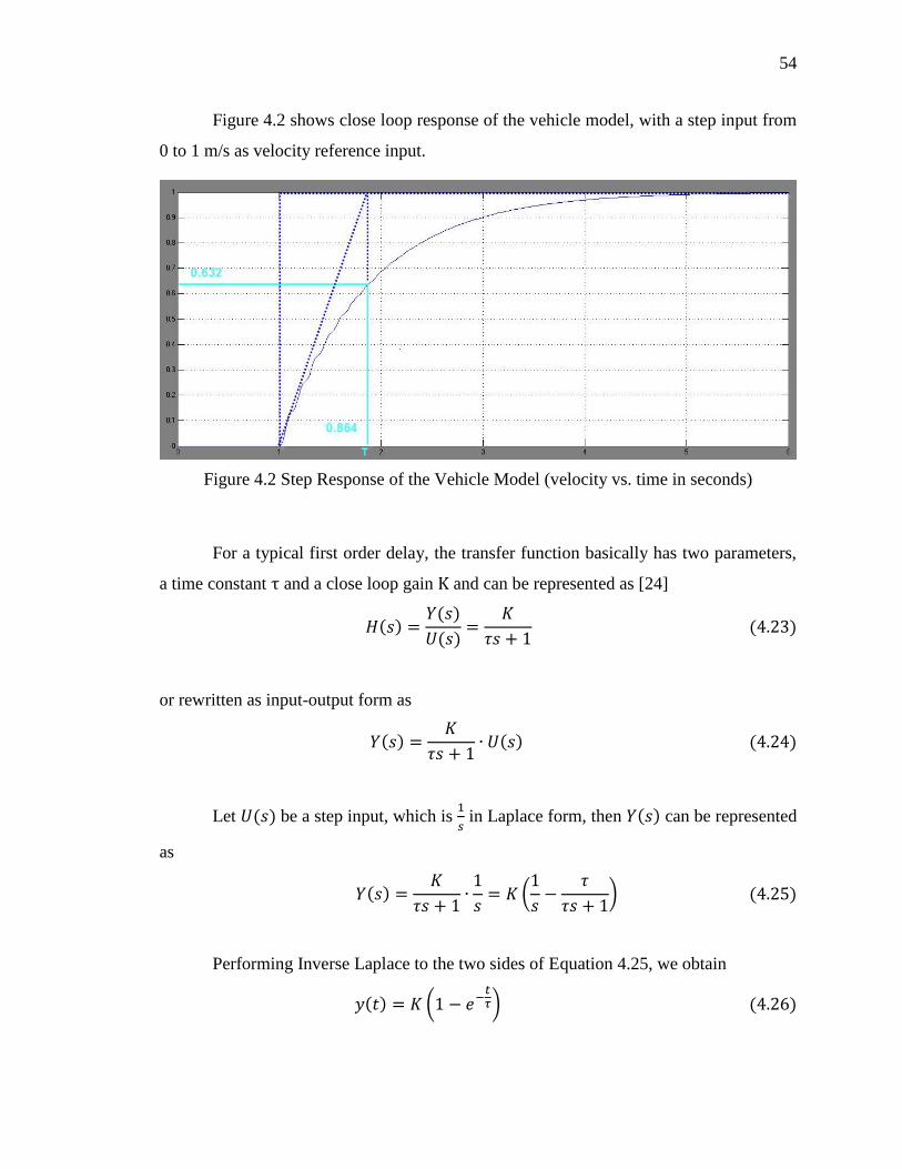
Figure 4.2 shows close loop response of the vehicle model, with a step input from
0 to 1 m/s as velocity reference input.
Figure 4.2 Step Response of the Vehicle Model (velocity vs. time in seconds)
For a typical first order delay, the transfer function basically has two parameters,
a time constant and a close loop gain and can be represented as [24]
or rewritten as input-output form as
Let be a step input, which is
in Laplace form, then can be represented
as
(
)
Performing Inverse Laplace to the two sides of Equation 4.25, we obtain
( )
55
Let t = and K = 1, from Equation 4.26,
It can be clearly recognized that a first order delay is characterized in the step
response and by measuring the corresponding time at magnitude of 63.2% of the step
response [25]. From Equation 4.27, the time constant of the first order delay can be
estimated, which is equal to 0.864s. Therefore a component of the dynamic system can be
written as a first order delay with time constant s, shown as follows:
where and unknown.
Observing the step response, it’s not difficult to notice that there are small waves
around the beginning part of the response, which are caused by the other pole with a
much smaller time constant, because when looking on a larger time scale, the influence of
the pole with smaller time constant is limited and even hardly noticeable.
Using the Matlab System Identification toolbox, the other time constant is
estimated to be 0.002, exactly as what has been predicted, a much smaller time constant
than that of the first order component. Since the pole corresponding to time constant is
much farther away from the vertical axis in a complex plane than that corresponding to
time constant (more than 10 times farther way), its influence to the whole system can
be neglected when looking on a large scale in time.
4.3.1. Desired Headway Distance Based on Velocity of The Preceding Vehicle
As described in Section 4.1.1, the implementation of desired headway distance
based on the velocity of the preceding vehicle is more straight-forward. In this section,
two conditions are derived from what has been discussed above for this type of
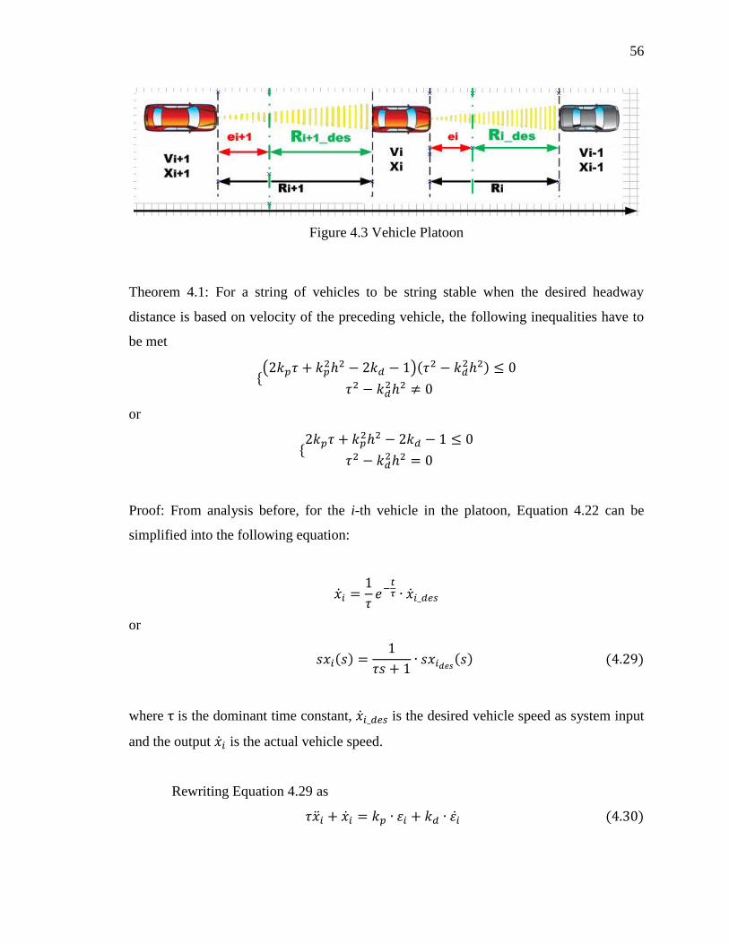
implementation, as shown in Figure 4.3.
56
Figure 4.3 Vehicle Platoon
Theorem 4.1: For a string of vehicles to be string stable when the desired headway
distance is based on velocity of the preceding vehicle, the following inequalities have to
be met
(
)
or
Proof: From analysis before, for the i-th vehicle in the platoon, Equation 4.22 can be
simplified into the following equation:
or
where is the dominant time constant, is the desired vehicle speed as system input
and the output is the actual vehicle speed.
Rewriting Equation 4.29 as
57
where is the spacing error of the i-the vehicle, and are the parameters of the PD
controller for headway control, and serves as control input [26].
From Equation 4.30, change the index of each term from i to i-1,
From the definition of spacing error, refer to Figure 4.3,
Differentiating the two sides of Equation 4.32 yields
Rewriting Equation 4.32 and Equation 4.33, one obtains
( )
Substituting and in Equation 4.31 for Equation 4.34 yields
( )
Taking Laplace Transform to the equation, we obtain
Changing the index of each term in Equation 4.32 from i to i-1 yield
Subtracting the two sides of Equation 4.32 from the two sides of Equation 4.36,
one obtains
58
Performing Laplace transform to Equation 4.37, we obtain
Substituting in Equation 4.38 for Equation 4.35 and rearranging the two
sides yields
(
)
Changing the index of Equation 4.39 from i-1 to i, we obtain
(
)
Substituting and in Equation 4.38 for Equation 4.39 and Equation
4.40, the error transfer function could be derived as
( )
From Section 4.2, for a platoon of vehicle to maintain string stability, the norm of
error transfer function has to be less or equal to 1 for any angular frequency , therefore,
| | |
|
Then the following equation can be derived from the above condition,
The above inequality has to hold for all to ensure string stability, which
requires that
59
then the following conditions can be derived,
(
)
or
4.3.2. Desired Headway Distance Based on Velocity of The Following Vehicle
As discussed in Section 4.1.2, a different definition of desired headway distance
would lead to different conditions for string stability. In Section 4.3.1, conditions for the
first case have been derived, while in this section, condition for the second case will be
discussed.
Theorem 4.2: For a string of vehicles to be string stable when the desired headway
distance is based on velocity of the preceding vehicle, the following inequalities have to
be met
Proof: Equation 4.23 and Equation 4.24 still hold in this case. Different definition of
desired headway distance leads to a different definition of headway spacing error of the i-
th vehicle, which is shown as follows,
Differentiating the two sides of Equation 4.45 yields
Equation 4.45 and Equation 4.46 can be rewritten as follows:
60
( )
Substituting and in Equation 4.24 for Equation 4.47, we obtain
( )
By rearranging the two sides of the Equation 4.48 and performing Laplace
transform, one obtains
Changing the index of Equation 4.46 and Equation 4.49 from i to i-1 yields
Subtracting the two sides of Equation 4.46 from the two sides of Equation 4.50,
we obtain
Substituting and in Equation 4.52 for Equation 4.49 and Equation
4.51, the error transfer function could be derived as follows,
( )
From Section 4.2, for a platoon of vehicle to maintain string stability, the norm of
error transfer function has to be less or equal to 1 for any angular frequency , therefore
| | |
|
61
The following equation can be derived from the above condition,
|
( )
|
⇒
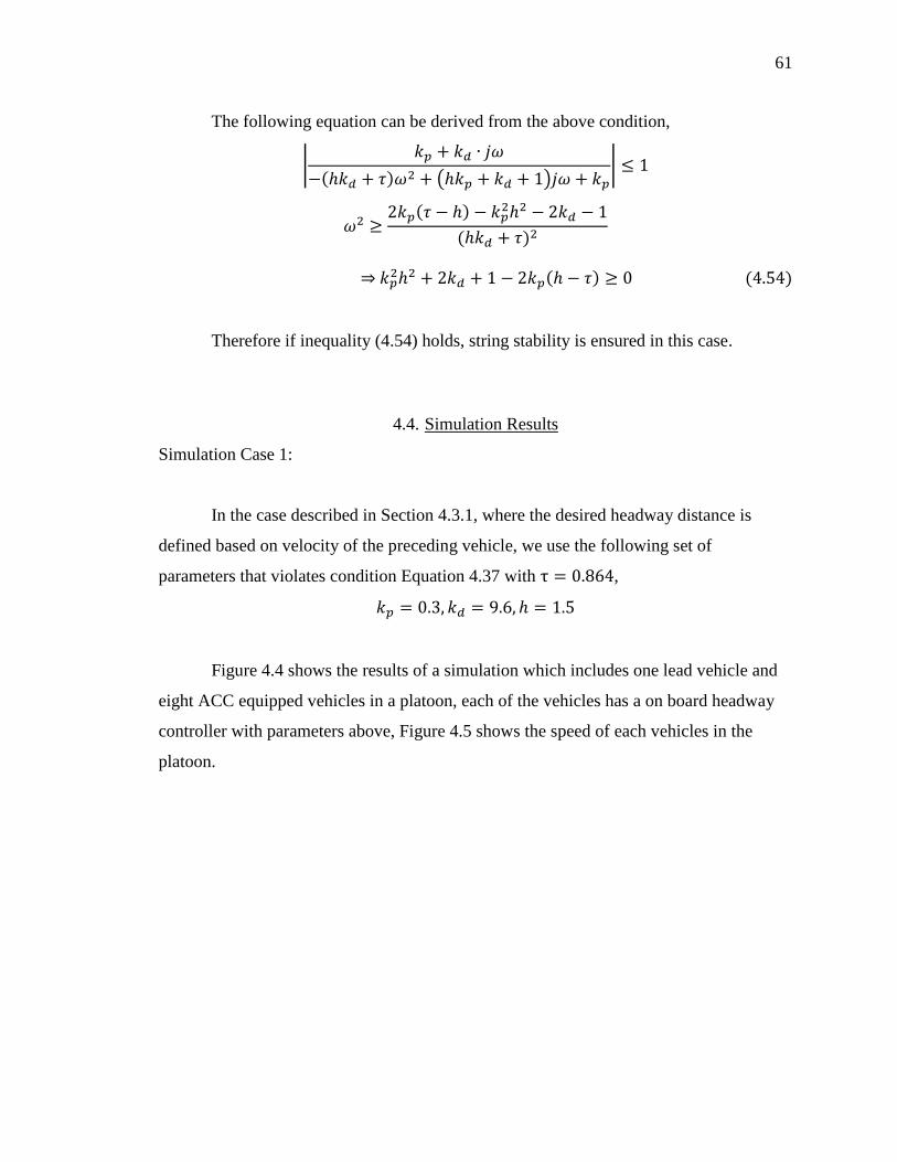
Therefore if inequality (4.54) holds, string stability is ensured in this case.
4.4. Simulation Results
Simulation Case 1:
In the case described in Section 4.3.1, where the desired headway distance is
defined based on velocity of the preceding vehicle, we use the following set of
parameters that violates condition Equation 4.37 with ,
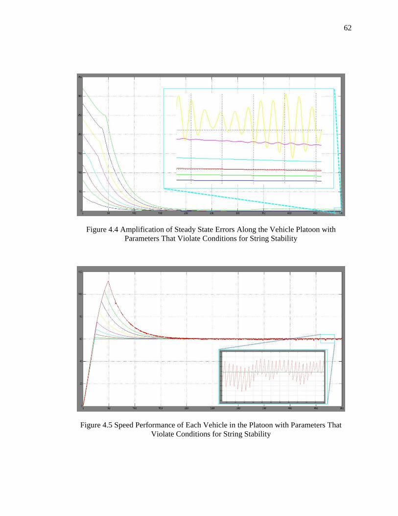
Figure 4.4 shows the results of a simulation which includes one lead vehicle and
eight ACC equipped vehicles in a platoon, each of the vehicles has a on board headway
controller with parameters above, Figure 4.5 shows the speed of each vehicles in the
platoon.
62
Figure 4.4 Amplification of Steady State Errors Along the Vehicle Platoon with
Parameters That Violate Conditions for String Stability
Figure 4.5 Speed Performance of Each Vehicle in the Platoon with Parameters That
Violate Conditions for String Stability

63
Simulation Case 2:
Then we try to use another set of parameters that satisfies condition (4.38), which
is
Then there should be no amplification of steady state errors, shown in Figure 4.6, and
Figure 4.7 shows the speed performance of each vehicle. This simulation shows results
that is exactly as what has been theoretically predicted.
Figure 4.6 Amplification of Steady State Errors along the Vehicle Platoon with
Parameters That Satisfy Conditions for String Stability

64
Figure 4.7 Speed Performance of Each Vehicle in the Platoon with Parameters That
Satisfy Conditions for String Stability
4.5. Chapter Summary
In this chapter, the definition of string stability in a platoon of vehicles was
discussed and mathematically described. General conditions for string stability have been
derived. Conditions of string stability in steady state for two common implementations
have also been discussed and mathematically derived.
65
5. CONCLUSION
In this thesis, we studied the algorithms of Adaptive Cruise Control (ACC) for
common passenger vehicles and systematic pressures have been developed for
implementations of such controller. In addition, string stability issues of a platoon of
vehicles which are equipped with ACC controller have been discussed.
A longitudinal model of vehicle dynamic has been designed and verified on
Matlab/Simulink environment. The vehicle dynamic equations depend on the longitudinal
tire forces, aerodynamic drag forces, rolling resistance force and gravitational force. A
systematic way to design ACC algorithms has been discussed in details. R-Rdot chart has
been introduced to assist the design process. Constant deceleration of the following
vehicle has been discussed to achieve a faster process to the equilibrium point, i.e. the
desired headway distance to the preceding vehicle. Two constant deceleration levels have
been chosen to be the upper limit and lower limit for the switching zone on an R-Rdot
chart, according to the maximum deceleration level which human beings normally feel
comfortable with. Simulations have shown a faster elapsed time than conventional design
of ACC system, and maintained driving safety at the same time.
The string stability issues in situations where when many vehicles with ACC
controller forming a vehicle platoon have been investigated. A generation of string
stability of interconnected vehicles has been addressed and mathematically described.
According to different definitions of desired headway distance, headway distance based
on velocity of the preceding vehicle and based on that of the following vehicle, different
conditions have been derived corresponding to each situation, respectively.
66
Corresponding to each case, simulations have been conducted and the results are
quite satisfactory indeed.
Possible future works involve (1) using advanced control algorithms instead of
PID to improve performance, (2) using more aggressive switching logic to further shorten
elapsed time during transient process, and (3) taking sensor noise influence into
consideration.

LIST OF REFERENCES
67
LIST OF REFERENCES
[1] P. Fancher, et al., “Intelligent cruise control field operational test,” DOT HS, vol.
808, p. 849, 1998.
[2] J. Woll, "Radar-based adaptive cruise control for truck applications,"
International Truck & Bus Meeting & Exposition, Nov. 1997.
[3] D. Swaroop, J.K. Hedrick, "String stability of interconnected systems," IEEE
Trans. Automatic Control., vol. 41, no. 3, pp. 349-357, Mar. 1996.
[4] J.K. Hedrick, D. McMahon, D. Swaroop, "Vehicle modeling and control for
automated highway systems," PATH Report, Institute of Transportation Studies,
UC Berkeley, UCB-ITS-PRP-93-24, Nov. 1993.
[5] J.K. Hedrick, D. McMahon, V. Narendran, D. Swaroop, "Longitudinal vehicle
controller design for IVHS systems," American Control Conference, pp.
3107-3112, 1991.
[6] D. Swaroop, et al., “A Comparision of Spacing and Headway Control Laws for
Automatically Controlled Vehicles,” Vehicle System Dynamics, vol. 23, pp.
597-625, 1994.
[7] Reichart, G., Haller, R., Naab, K., "Driver assistance: BMW solutions for the
future of individual mobility," in Proc. of ITS World Congress, 1996.
[8] D. Swaroop and J. Hedrick, “String stability of interconnected systems,” IEEE
Transactions on Automatic Control, vol. 41, pp. 349 - 357, 1996.
[9] R. Rajamani and C. Zhu, “Semi-autonomous adaptive cruise control systems,”
IEEE Transitions on Vehicular Technology, vol. 51, pp. 1186 - 1192, 2002.
68
[10] “A Compilation of Motor Vehicle Crash Data from the Fatal Accident Reporting
System and the General Estimates System,” US Department of Transportation,
National Highway Traffic Safety Administration, p. 50, 1994.
[11] 余志生, 汽车理论, 第三版. 北京: 机械工业出版社, 2005. (Zhisheng Yu,
Automobile Theory, Third Edition, Beijing: China Machine Press, 2005).
[12] R. Rajamani, Vehicle dynamics and control, Springer, 2006.
[13] E. Hendricks and S. Sorenson, “Mean value modeling of spark ignition engines,”
International Congress & Exposition, 1990.
[14] Mathworks, Gasoline Engine Block Online Help Documents. Available:
http://www.mathworks.com/help/toolbox/physmod/drive/gasolineengine.html.
[15] D. Cho and J. Hedrick, “Automotive powertrain modeling for control,” Journal of
Dynamic Systems, Measurement, and Control, vol. 111, p. 568, 1989.
[16] A. Tugcu, et al., “Modeling and simulation of the powertrain dynamics of
vehicles equipped with automatic transmission,” pp. 39-61, 1987.
[17] J. Runde, Modeling and Control of an Automatic Transmission, Massachusetts
Institute of Technology, 1986.
[18] H. Pacejka, “The tyre as a vehicle component,” XXVI FISITA Congress, 1996.
[19] Mathworks, Simulink Tire Model Online Help Documents. Available:
http://www.mathworks.com/help/toolbox/physmod/drive/tire.html
[20] P. Ioannou and C. Chien, “Autonomous intelligent cruise control,” IEEE
Transactions on Vehicular Technology, vol. 42, pp. 657-672, 1993.
[21] P. Fancher and Z. Bareket, "Evaluating headway control using range versus
range-rate relationships," Vehicle System Dynamics, vol. 23, no. 1, pp. 575-596,
1994.
[22] P. Fancher, et al., “Intelligent cruise control: Performance studies based upon an
operating prototype,” 1994, pp. 391-399.
69
[23] C. Desoer and M. Vidyasagar, Feedback Systems: Input-Output Properties,
Society for Industrial and Applied Mathematics, 2009.
[24] 徐薇莉, 曹柱中, 田作华, 自动控制理论与设计, 第三版: 上海交通大学出版
社, 1995. (W. Xu, Z. Cao, and Z. Tian, Automotive Control Theory and Design,
Third Edition: Shanghai Jiaotong University Press, 1995.)
[25] K. Ogata, Modern Control Engineering, Prentice Hall, 2009.
[26] K. Astrom and T. Hagglund, PID Controllers: Theory, Design, and Tuning,
Second Edition, International Society for Measurement and Control, 1995.