gps group 9 project

GPS Group Project ENAE441 Fall 2012

Group 9 Marco Colleluori Mike Hamilton Thomas Noyes Matthew Rich

1. Problem Statement

The ultimate goal of this project is to determine the location of a ‘receiver’ site on the surface of the Earth. Intermediate steps necessary to achieve this goal include the calculation of satellite ‘orbit in time’ data using orbital elements and related data and the design and validation of code used to calculate the Earth surface location of an observer site or ‘receiver’. Three Receiver Independent Exchange (RINEX) data sets are provided: 1) A NAV set which provides the orbital parameters, observation time and time corrections, and harmonic corrections for a set of satellites observed on November 6, 2012; 2) A set of satellite observation data (OBS) from a known Continuously Operating Reference Station (CORS); 3) A set of satellite observation data (OBS) from an unknown International GNSS Service (IGS) site.

Data set one is used to calculate satellite ‘orbit in time’ information for the satellites under observation in the CORS and IGS data sets.

Data set two is used to verify and validate the code used to determine the Earth surface location of the ‘receiver’. The location of this ‘receiver’ is provided for comparison with the calculated results to verify accuracy.

Data set three is used to determine the Earth surface location of an unknown ‘receiver’ site.

The algorithm described within Elliott Kaplan’s “Understanding GPS: Principles and Applications” on page 38 was used to determine each satellite’s ECEF position vector in time. The algorithm described within Dr. Liam Healy’s ENAE441 course notes on page 510 was used to calculate the observer’s site vector.

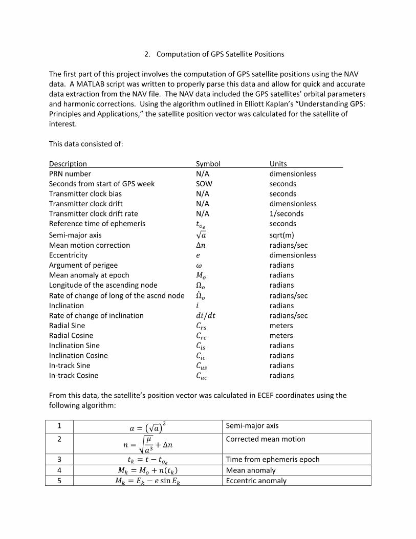
2. Computation of GPS Satellite Positions

The first part of this project involves the computation of GPS satellite positions using the NAV data. A MATLAB script was written to properly parse this data and allow for quick and accurate data extraction from the NAV file. The NAV data included the GPS satellites’ orbital parameters and harmonic corrections. Using the algorithm outlined in Elliott Kaplan’s “Understanding GPS: Principles and Applications,” the satellite position vector was calculated for the satellite of interest. This data consisted of: Description Symbol Units PRN number N/A dimensionless Seconds from start of GPS week SOW seconds Transmitter clock bias N/A seconds Transmitter clock drift N/A dimensionless Transmitter clock drift rate N/A 1/seconds Reference time of ephemeris

seconds

Semi-major axis √ sqrt(m) Mean motion correction radians/sec Eccentricity dimensionless Argument of perigee radians Mean anomaly at epoch radians Longitude of the ascending node radians

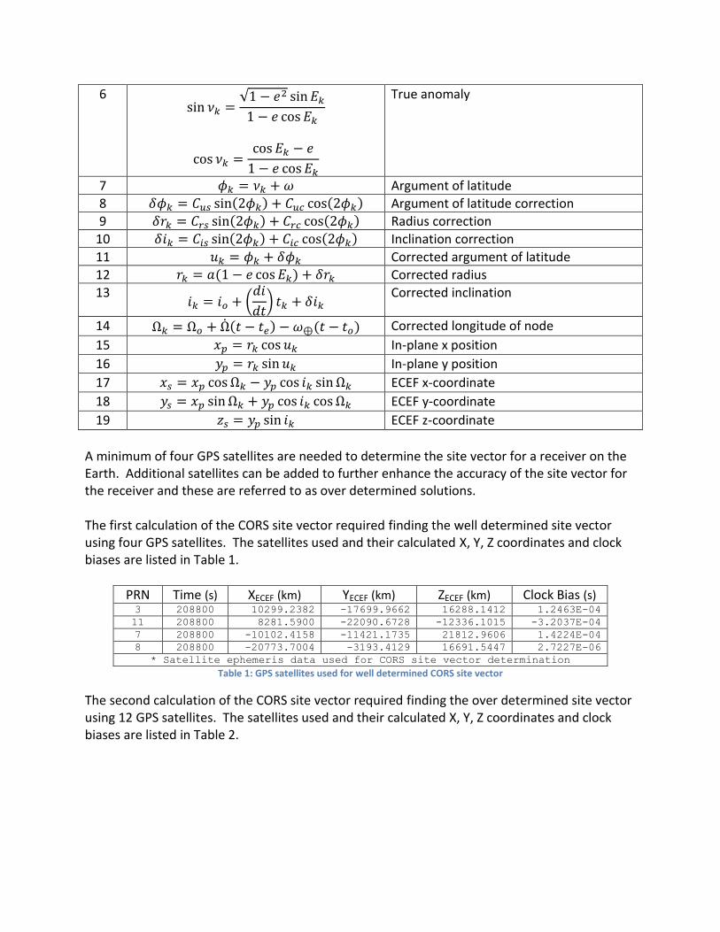
Rate of change of long of the ascnd node radians/sec Inclination radians Rate of change of inclination radians/sec Radial Sine meters Radial Cosine meters Inclination Sine radians Inclination Cosine radians In-track Sine radians In-track Cosine radians From this data, the satellite’s position vector was calculated in ECEF coordinates using the following algorithm:

1 (√ ) Semi-major axis

2 √

Corrected mean motion

3 Time from ephemeris epoch

4 ( ) Mean anomaly

5 Eccentric anomaly

6

√

True anomaly

7 Argument of latitude

8 ( ) ( ) Argument of latitude correction

9 ( ) ( ) Radius correction

10 ( ) ( ) Inclination correction

11 Corrected argument of latitude

12 ( ) Corrected radius

13 (

)

Corrected inclination

14 ( ) ( ) Corrected longitude of node

15 In-plane x position

16 In-plane y position

17 ECEF x-coordinate

18 ECEF y-coordinate

19 ECEF z-coordinate

A minimum of four GPS satellites are needed to determine the site vector for a receiver on the Earth. Additional satellites can be added to further enhance the accuracy of the site vector for the receiver and these are referred to as over determined solutions. The first calculation of the CORS site vector required finding the well determined site vector using four GPS satellites. The satellites used and their calculated X, Y, Z coordinates and clock biases are listed in Table 1.

Table 1: GPS satellites used for well determined CORS site vector

The second calculation of the CORS site vector required finding the over determined site vector using 12 GPS satellites. The satellites used and their calculated X, Y, Z coordinates and clock biases are listed in Table 2.

PRN Time (s) XECEF (km) YECEF (km) ZECEF (km) Clock Bias (s) 3 208800 10299.2382 -17699.9662 16288.1412 1.2463E-04

11 208800 8281.5900 -22090.6728 -12336.1015 -3.2037E-04

7 208800 -10102.4158 -11421.1735 21812.9606 1.4224E-04

8 208800 -20773.7004 -3193.4129 16691.5447 2.7227E-06

* Satellite ephemeris data used for CORS site vector determination

Table 2: GPS satellites used for over determined CORS site vector

Lastly, the calculation of the IGS site vector required finding the over determined site vector using 12 GPS satellites. The satellites used and their calculated X, Y, Z coordinates and clock biases are listed in Table 3.

Table 3: GPS satellites used for over determined IGS site vector

PRN Time (s) XECEF (km) YECEF (km) ZECEF (km) Clock Bias (s) 3 209400 10618.9515 -16376.4016 17410.0880 1.2464E-04

6 209400 14035.9460 -10218.0668 20115.3665 4.6525E-04

7 209400 -8643.4861 -12213.1130 21993.6406 1.4224E-04

11 209400 9072.0141 -22525.9284 -10833.4510 -3.2037E-04

13 209400 -5380.2722 -23405.8483 11082.6871 1.6920E-04

16 209400 15535.6195 -6486.9209 20619.6322 -2.4914E-04

1 219330 14154.7188 -19784.7796 10569.8217 2.8118E-04

7 219330 6070.5817 -25431.2592 3732.8626 1.4228E-04

8 219330 -1572.5761 -21219.2547 15591.3738 2.7249E-06

19 219330 17049.9642 -988.9773 20366.3791 -3.1971E-04

26 219330 -19490.0943 -8879.9478 15310.9563 -2.1978E-04

28 219330 -9154.9835 -13257.4212 21722.7257 2.0209E-04

* Satellite ephemeris data used for CORS site vector determination

PRN Time (s) XECEF (km) YECEF (km) ZECEF (km) Clock Bias (s) 2 212700 -21407.0026 12059.1386 -9254.4832 4.0813E-04

9 212700 -15288.5186 20996.4242 -6255.8804 1.9779E-04

12 212700 -5722.5105 13651.1141 -22064.2346 1.0015E-04

14 212700 13704.8248 16560.9162 -15498.9501 2.1625E-04

2 216000 -18708.2283 6798.3012 -17182.6372 4.0813E-04

9 216000 -15994.0940 20692.7507 4267.6771 1.9779E-04

12 216000 -14266.8402 11829.4635 -18968.2784 1.0016E-04

14 216000 14456.4518 21332.0212 -6545.7742 2.1625E-04

15 216000 -10559.8380 12269.0196 21014.3448 -9.8993E-05

18 216000 7334.4216 15683.3711 20599.8756 2.2329E-04

21 216000 784.9253 21266.2825 16061.2225 -2.6052E-04

25 216000 -578.9280 15002.3479 -21946.9613 4.9818E-05

* Satellite ephemeris data used for IGS site vector determination

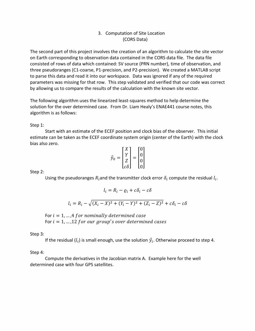
3. Computation of Site Location (CORS Data)

The second part of this project involves the creation of an algorithm to calculate the site vector on Earth corresponding to observation data contained in the CORS data file. The data file consisted of rows of data which contained: SV source (PRN number), time of observation, and three pseudoranges (C1-coarse, P1-precision, and P2-precision). We created a MATLAB script to parse this data and read it into our workspace. Data was ignored if any of the required parameters was missing for that row. This step validated and verified that our code was correct by allowing us to compare the results of the calculation with the known site vector. The following algorithm uses the linearized least-squares method to help determine the solution for the over determined case. From Dr. Liam Healy’s ENAE441 course notes, this algorithm is as follows: Step 1: Start with an estimate of the ECEF position and clock bias of the observer. This initial estimate can be taken as the ECEF coordinate system origin (center of the Earth) with the clock bias also zero.

[

] [

]

Step 2: Using the pseudoranges and the transmitter clock error compute the residual .

√( ) ( ) ( )

For For

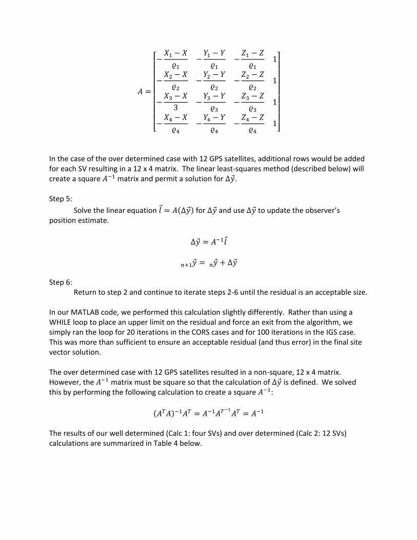
Step 3: If the residual ( ) is small enough, use the solution . Otherwise proceed to step 4. Step 4: Compute the derivatives in the Jacobian matrix A. Example here for the well determined case with four GPS satellites.

[

]

In the case of the over determined case with 12 GPS satellites, additional rows would be added for each SV resulting in a 12 x 4 matrix. The linear least-squares method (described below) will create a square matrix and permit a solution for . Step 5:

Solve the linear equation ( ) for and use to update the observer’s position estimate.

Step 6: Return to step 2 and continue to iterate steps 2-6 until the residual is an acceptable size. In our MATLAB code, we performed this calculation slightly differently. Rather than using a WHILE loop to place an upper limit on the residual and force an exit from the algorithm, we simply ran the loop for 20 iterations in the CORS cases and for 100 iterations in the IGS case. This was more than sufficient to ensure an acceptable residual (and thus error) in the final site vector solution. The over determined case with 12 GPS satellites resulted in a non-square, 12 x 4 matrix. However, the matrix must be square so that the calculation of is defined. We solved this by performing the following calculation to create a square :

( )

The results of our well determined (Calc 1: four SVs) and over determined (Calc 2: 12 SVs) calculations are summarized in Table 4 below.

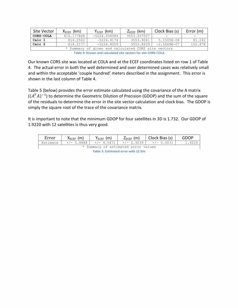
Table 4: Known and calculated site vectors for site CORS-COLA

Our known CORS site was located at COLA and at the ECEF coordinates listed on row 1 of Table 4. The actual error in both the well determined and over determined cases was relatively small and within the acceptable ‘couple hundred’ meters described in the assignment. This error is shown in the last column of Table 4. Table 5 (below) provides the error estimate calculated using the covariance of the A matrix (( ) ) to determine the Geometric Dilution of Precision (GDOP) and the sum of the square of the residuals to determine the error in the site vector calculation and clock bias. The GDOP is simply the square root of the trace of the covariance matrix. It is important to note that the minimum GDOP for four satellites in 3D is 1.732. Our GDOP of 1.9220 with 12 satellites is thus very good.

Table 5: Estimated error with 12 SVs

Site Vector XECEF (km) YECEF (km) ZECEF (km) Clock Bias (s) Error (m) CORS-COLA 816.177848 -5224.934084 3553.937007 - -

Calc 1 816.2502 -5224.9174 3553.9041 5.1505E-08 81.242

Calc 2 816.2177 -5224.8059 3553.8639 -2.5669E-07 152.878

* Summary of given and calculated CORS site vectors

Error XECEF (m) YECEF (m) ZECEF (m) Clock Bias (s) GDOP Estimate +/- 0.8888 +/- 4.5471 +/- 2.9239 +/- 0.0031 1.9220

* Summary of estimated error values

4. Computation of Site Location (IGS Data)

The third and final part of this project involved the calculation of an unknown site vector using the data contained in the IGS data file. This data file was formatted in an identical manner to the CORS file, and we were able to use a similar MATLAB script to parse and extract the data into our workspace. This time however we used a time in the middle of the data set as well as data from both the L1 and L2 carrier frequencies. By using a time in the middle of the data set, we were forced to propagate the position of the satellites. With the above modifications, we used the same algorithm and calculations described in the previous section with 12 SVs (the over determined case). This time however we iterated 100 times through the update algorithm to ensure that a sufficiently small residual would result.

Table 6: Unknown site vector determination from IGS data using 12 SVs

We determined that the observations were made from the IGS site BAKO in Cibinong, West Java, Indonesia. The location is displayed on a map in Figure 1. Again, the actual error in the site determination and clock bias is very good, as is the error estimate and the GDOP. In fact, the error in the IGS calculation is significantly smaller (less than 50%) than the error in the CORS calculations.

Table 7: Error estimate in IGS site vector calculation using 12 SVs

Site Vector XECEF (km) YECEF (km) ZECEF (km) Clock Bias

(s) Error (m) IGS-BAKO -1836.969054 6065.617126 -716.257839 - -

L1 Calc -1837.0315 6065.6098 -716.2317 1.3364E-07 68.0738

L2 Calc -1837.0334 6065.6093 -716.2313 1.4177E-07 70.007

* Summary of determined and calculated IGS site vectors

Error XECEF (m) YECEF (m) ZECEF (m) Clock Bias (s) GDOP L1 Est. +/- 0.5125 +/- 3.5970 +/- 0.2959 +/- 0.0010 1.9353

L2 Est. +/- 0.5041 +/- 3.5377 +/- 0.2910 +/- 0.0010 1.9353


IGS Site Vector Results

City or Town : Cibinong

State or Province : West Java

Country : Indonesia

Figure 1: Location of the IGS observation site

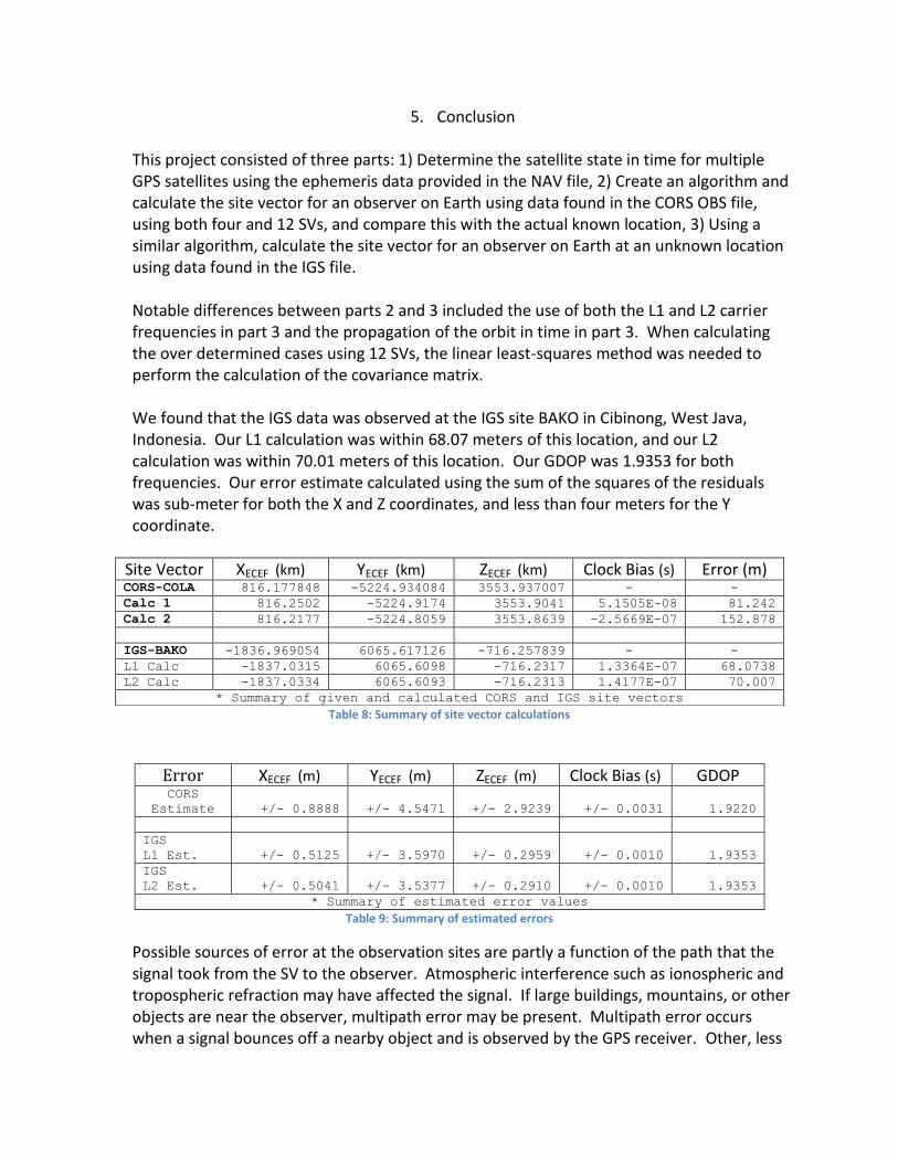
5. Conclusion This project consisted of three parts: 1) Determine the satellite state in time for multiple GPS satellites using the ephemeris data provided in the NAV file, 2) Create an algorithm and calculate the site vector for an observer on Earth using data found in the CORS OBS file, using both four and 12 SVs, and compare this with the actual known location, 3) Using a similar algorithm, calculate the site vector for an observer on Earth at an unknown location using data found in the IGS file. Notable differences between parts 2 and 3 included the use of both the L1 and L2 carrier frequencies in part 3 and the propagation of the orbit in time in part 3. When calculating the over determined cases using 12 SVs, the linear least-squares method was needed to perform the calculation of the covariance matrix. We found that the IGS data was observed at the IGS site BAKO in Cibinong, West Java, Indonesia. Our L1 calculation was within 68.07 meters of this location, and our L2 calculation was within 70.01 meters of this location. Our GDOP was 1.9353 for both frequencies. Our error estimate calculated using the sum of the squares of the residuals was sub-meter for both the X and Z coordinates, and less than four meters for the Y coordinate.

Table 8: Summary of site vector calculations

Table 9: Summary of estimated errors

Possible sources of error at the observation sites are partly a function of the path that the signal took from the SV to the observer. Atmospheric interference such as ionospheric and tropospheric refraction may have affected the signal. If large buildings, mountains, or other objects are near the observer, multipath error may be present. Multipath error occurs when a signal bounces off a nearby object and is observed by the GPS receiver. Other, less

Site Vector XECEF (km) YECEF (km) ZECEF (km) Clock Bias (s) Error (m) CORS-COLA 816.177848 -5224.934084 3553.937007 - -

Calc 1 816.2502 -5224.9174 3553.9041 5.1505E-08 81.242

Calc 2 816.2177 -5224.8059 3553.8639 -2.5669E-07 152.878

IGS-BAKO -1836.969054 6065.617126 -716.257839 - -

L1 Calc -1837.0315 6065.6098 -716.2317 1.3364E-07 68.0738

L2 Calc -1837.0334 6065.6093 -716.2313 1.4177E-07 70.007

* Summary of given and calculated CORS and IGS site vectors

Error XECEF (m) YECEF (m) ZECEF (m) Clock Bias (s) GDOP CORS

Estimate +/- 0.8888 +/- 4.5471 +/- 2.9239 +/- 0.0031 1.9220

IGS

L1 Est. +/- 0.5125 +/- 3.5970 +/- 0.2959 +/- 0.0010 1.9353

IGS

L2 Est. +/- 0.5041 +/- 3.5377 +/- 0.2910 +/- 0.0010 1.9353


significant sources of error include noise in the receiver and phase center variation. Because the GDOP was so low, the error resulting from the spread of the satellites was minimal. Our calculation did take into account clock biases and drift, so these should not have played a significant role in the error. We may have been able to reduce the error by using a Kalman filter instead of the linear least-squares method. This would have allowed us to take into account the signal noise and variability in the GPS signals. More accurate results are possible if differential GPS (DGPS) is used. DGPS uses known ground stations to broadcast telemetry. Nearby receivers can use this broadcast and the error calculations it contains to correct the GPS signals they receive. This can result in very precise (sub-meter) accuracy.

6. Appendix (MATLAB Code)

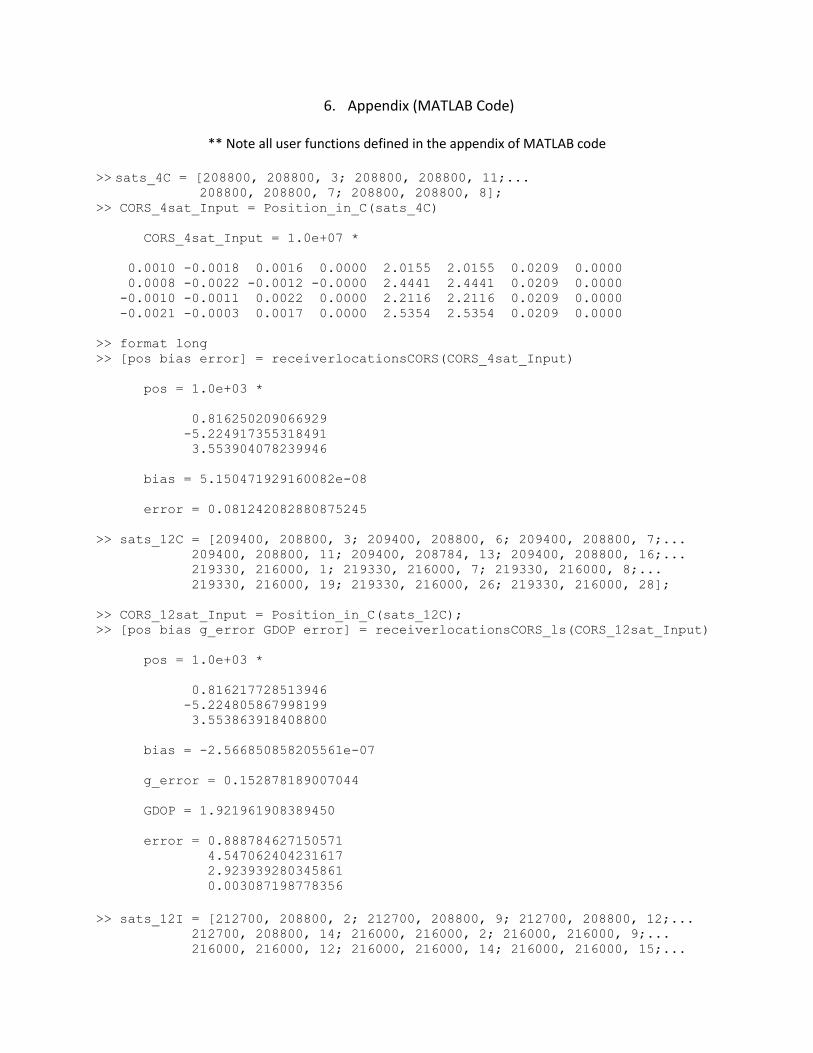
** Note all user functions defined in the appendix of MATLAB code >> sats_4C = [208800, 208800, 3; 208800, 208800, 11;... 208800, 208800, 7; 208800, 208800, 8];

>> CORS_4sat_Input = Position_in_C(sats_4C)

CORS_4sat_Input = 1.0e+07 *

0.0010 -0.0018 0.0016 0.0000 2.0155 2.0155 0.0209 0.0000

0.0008 -0.0022 -0.0012 -0.0000 2.4441 2.4441 0.0209 0.0000

-0.0010 -0.0011 0.0022 0.0000 2.2116 2.2116 0.0209 0.0000

-0.0021 -0.0003 0.0017 0.0000 2.5354 2.5354 0.0209 0.0000

>> format long

>> [pos bias error] = receiverlocationsCORS(CORS_4sat_Input)

pos = 1.0e+03 *

0.816250209066929

-5.224917355318491

3.553904078239946

bias = 5.150471929160082e-08

error = 0.081242082880875245

>> sats_12C = [209400, 208800, 3; 209400, 208800, 6; 209400, 208800, 7;...

209400, 208800, 11; 209400, 208784, 13; 209400, 208800, 16;...

219330, 216000, 1; 219330, 216000, 7; 219330, 216000, 8;...

219330, 216000, 19; 219330, 216000, 26; 219330, 216000, 28];

>> CORS_12sat_Input = Position_in_C(sats_12C);

>> [pos bias g_error GDOP error] = receiverlocationsCORS_ls(CORS_12sat_Input)

pos = 1.0e+03 *

0.816217728513946

-5.224805867998199

3.553863918408800

bias = -2.566850858205561e-07

g_error = 0.152878189007044

GDOP = 1.921961908389450

error = 0.888784627150571

4.547062404231617

2.923939280345861

0.003087198778356

>> sats_12I = [212700, 208800, 2; 212700, 208800, 9; 212700, 208800, 12;...

212700, 208800, 14; 216000, 216000, 2; 216000, 216000, 9;...

216000, 216000, 12; 216000, 216000, 14; 216000, 216000, 15;...

216000, 216000, 18; 216000, 216000, 21; 216000, 216000, 25];

>> IGS_12sat_Input = Position_in_I(sats_12I);

>> [L1 bias1 GDOP1 err1 L2 bias2 GDOP2 err2] =

receiverlocationsIGS_ls(IGS_12sat_Input)

L1 = 1.0e+03 *

-1.837031467133219

6.065609787766618

-0.716231670360575

bias1 = 1.336439782907477e-07

GDOP1 = 1.935269567622818

err1 = 0.512543635831831

3.596950296278345

0.295861967230292

0.001047449534270

L2 = 1.0e+03 *

-1.837033355134456

6.065609260657103

-0.716231298230505

bias2 = 1.417722762048748e-07

GDOP2 = 1.935269518503820

err2 = 0.504094316862999

3.537654498653472

0.290984702563833

0.001030182418294

>> IGS_sv = [-1836.969054; 6065.617126; -716.257839];

>> g_error1 = norm(IGS_sv-L1)*1000

g_error1 = 68.073831659035022

>> g_error2 = norm(IGS_sv-L2)*1000

g_error2 = 70.006513672866589

Appendix of MATLAB Code

Kepler.m function [E] = Kepler(M, e)

if(M>pi)

E = M - e/2;

else

E = M + e/2;

end

ratio = 1;

while(ratio>(10e-4))

f1 = E - e*sin(E) - M;

f2 = 1 - e*cos(E);

ratio = f1/f2;

E = E - ratio;

end

end

sat_ECEF.m function [output] = sat_ECEF(ephem, obs)

% Define Constants

mu = 398600.4418; % gravitational constant

Om_e = 7.292115146e-5; % rotation rate of Earth

% Extract Parameters from input

PRN = ephem(1);

t_0e = ephem(2);

t = obs(1);

% Orbit Parameters

sqrt_a = ephem(4); % Square root of semimajor Axis (m^1/2)

dn = ephem(5); % Motion correction (rad/sec)

e = ephem(6); % Eccentricity

w = ephem(7); % Argument of perigee (rad)

M_0 = ephem(8); % Mean anomaly at epoch (rad)

Om_0 = ephem(9); % Right ascension (rad)

Om_dot = ephem(10); % Right ascension rate (rad/sec)

i_0 = ephem(11); % Inclination (rad)

i_dot = ephem(12); % Inclination rate (rad/sec)

% Corrections

C_rs = ephem(13); % Sine correction to orbital radial (m)

C_rc = ephem(14); % Cosine correction to orbital radial (m)

C_is = ephem(15); % Sine correction to inclination (rad)

C_ic = ephem(16); % Cosine correction to inclination (rad)

C_us = ephem(17); % Sine correction to in-track (rad)

C_uc = ephem(18); % Cosine correction to in-track (rad)

% Calculate ECEF Coordinates

a = sqrt_a^2/1000; % semimajor axis (km)

n = sqrt(mu/a^3) + dn; % corrected mean motion (rad/sec)

t_k = t - t_0e; % Time from Ephemeric epoch (secs)

bias = t_k*ephem(19)+ephem(3); % Bias T0 propogated forward depending

% on the propogated time and drift (secs)

M_k = M_0 + n*t_k; % Total Mean anomaly (rad)

M_k = mod(M_k,2*pi); % Normalized Mean anomoly (rad)

[E_k] = Kepler(M_k,e); % eccentric anomaly (rad)

v_k = atan2(sqrt(1-e^2)*sin(E_k),cos(E_k)-e); % true anomaly (rad)

phi_k = v_k + w; % Argument of latitude (rad)

dphi_k = C_us*sin(2*phi_k) + C_uc*cos(2*phi_k); % Corrected Argument of latitude (rad)

dr_k = (10^-3)*(C_rs*sin(2*phi_k) + C_rc*cos(2*phi_k)); % Radial correction (rad)

di_k = C_is*sin(2*phi_k) + C_ic*cos(2*phi_k); % Inclination correction (rad)

% Corrected values

u_k = phi_k + dphi_k; % Corrected argument of latitude (rad)

r_k = a*(1-e*cos(E_k)) + dr_k; % Corrected radius (km)

i_k = i_0 + i_dot*t_k + di_k; % Corrected inclination (rad)

Om_k = Om_0 + Om_dot*t_k - Om_e*t; % Corrected longitude of node (rad)

% PF Vectors

x_p = r_k*cos(u_k); % X_pf (km)

y_p = r_k*sin(u_k); % Y_pf (km)

% ECEF coordinates

X_s = x_p*cos(Om_k) - y_p*cos(i_k)*sin(Om_k); % (km)

Y_s = x_p*sin(Om_k) + y_p*cos(i_k)*cos(Om_k); % (km)

Z_s = y_p*sin(i_k); % [km]

output(1) = X_s;

output(2) = Y_s;

output(3) = Z_s;

output(4) = bias;

output(5) = obs(3);

output(6) = obs(4);

output(7) = t;

output(8) = obs(2);

end

searchCORS.m function [row] = searchCORS(time,satnum)

load('aero441proj')

for i=1:length(CORS)

if CORS(i,1)==time

if CORS(i,2)==satnum

row(1) = CORS(i,1);

row(2) = CORS(i,2);

row(3) = CORS(i,3);

row(4) = CORS(i,4);

end

end

end

end

searchIGS.m function [row] = searchIGS(time,satnum)

load('aero441proj')

for i=1:length(IGS)

if IGS(i,1)==time

if IGS(i,2)==satnum

row(1) = IGS(i,1);

row(2) = IGS(i,2);

row(3) = IGS(i,3);

row(4) = IGS(i,4);

end

end

end

end

readdata.m function [A] = readdata()

% Generate ID number for navigation file

fid=fopen('nov06.nav');

line=0;

i=0;

j=1;

% Loop through the entire file

while line~=-1

% Read text in line-by-line

line=fgets(fid);

% There are 46 lines per data set. Each relevant parameter appears a

% certain number of lines into each set and a certain number of

% characters into that line. Use the mod function to identify the

% relevant lines in the data set, then index by character in the line.

if mod(j,46)==4

i=i+1;

% PRN satellite number

A(i,1)=str2num(line(7:8));

elseif mod(j,46)==7

% SOW time


elseif mod(j,46)==21

% Bias T0



% Drift



% Semimajor axis



% Motion correction



% Eccentricity



% Argument of perigee



% Mean anomaly at epoch



% Right ascension


% Right ascension rate



% Inclination


% Inclination rate



% Amplitude of radial sine correction


% Amplitude of radial cosine correction



% Amplitude of inclination sine correction


% Amplitude of inclination cosine correction



% Amplitude of in-track sine correction


% Amplitude of in-track cosine correction


end

j=j+1;

end

% Close navigation file

fclose(fid);

end

searchNAV.m function out = searchNAV(time, satnum)

A = readdata();

[R,C] = size(A);

for i=1:R

if A(i,1)==satnum

if A(i,2)==time

for j=1:19

out(j) = A(i,j);

end

end

end

end

end

Position_in_C.m function [Posit] = Position_in_C(sats)

% sats is a Nx2 array of sat # and time

[R,C] = size(sats);

% Pick data from array

for j=1:R

ephem(j,:) = searchNAV(sats(j,2),sats(j,3));

end

% Get observation data

for i=1:R

obs(i,:) = searchCORS(sats(i,1),sats(i,3));

end

for k=1:R;

Posit(k,:) = sat_ECEF(ephem(k,:), obs(k,:));

end

end

Position_in_I.m function [Posit] = Position_in_I(sats)

% sats is a Nx2 array of sat # and time

[R,C] = size(sats);

% Pick data from array

for j=1:R

ephem(j,:) = searchNAV(sats(j,2),sats(j,3));

end

% Get observation data

for i=1:R

obs(i,:) = searchIGS(sats(i,1),sats(i,3));

end

for k=1:R;

Posit(k,:) = sat_ECEF(ephem(k,:), obs(k,:));

end

end

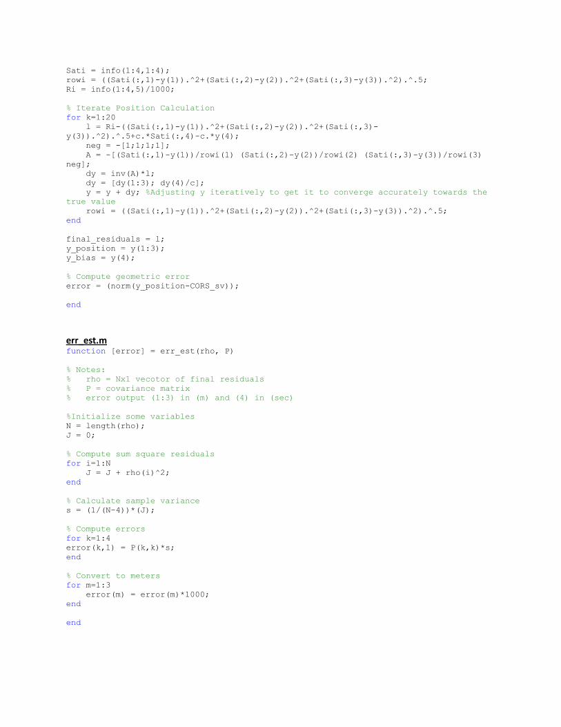
receiverlocationsCORS.m function [y_position y_bias error] = receiverlocationsCORS(info)

%% Receiver Locations

% A = matrix of derivatives

% c = signal speed (speed of light)

% d = clock bias

% di = satellite i clock bias

% l = residual from satellite

% rowi = range to satellite i

% Ri = pseudorange observed for satellite i

% Sati = matrix which holds information (Xi,Yi,Zi,c*di) for 4 satellites

% X,Y,Z = Receiver ECEF positions

% Xi,Yi,Zi = satellite i ECEF position

%% CORS Receiver Position - 4 Pseudo Ranges

% Known location

CORS_sv = [816.177848; -5224.934084; 3553.937007];

% Define constant

c = 3e5; % (km/s)

% Initialize Data

y = [0;0;0;0];

Sati = info(1:4,1:4);

rowi = ((Sati(:,1)-y(1)).^2+(Sati(:,2)-y(2)).^2+(Sati(:,3)-y(3)).^2).^.5;

Ri = info(1:4,5)/1000;

% Iterate Position Calculation

for k=1:20

l = Ri-((Sati(:,1)-y(1)).^2+(Sati(:,2)-y(2)).^2+(Sati(:,3)-

y(3)).^2).^.5+c.*Sati(:,4)-c.*y(4);

neg = -[1;1;1;1];

A = -[(Sati(:,1)-y(1))/rowi(1) (Sati(:,2)-y(2))/rowi(2) (Sati(:,3)-y(3))/rowi(3)

neg];

dy = inv(A)*l;

dy = [dy(1:3); dy(4)/c];

y = y + dy; %Adjusting y iteratively to get it to converge accurately towards the

true value


end

final_residuals = l;

y_position = y(1:3);

y_bias = y(4);

% Compute geometric error

error = (norm(y_position-CORS_sv));

end

err_est.m function [error] = err_est(rho, P)

% Notes:

% rho = Nx1 vecotor of final residuals

% P = covariance matrix

% error output (1:3) in (m) and (4) in (sec)

%Initialize some variables

N = length(rho);

J = 0;

% Compute sum square residuals

for i=1:N

J = J + rho(i)^2;

end

% Calculate sample variance

s = (1/(N-4))*(J);

% Compute errors

for k=1:4

error(k,1) = P(k,k)*s;

end

% Convert to meters

for m=1:3

error(m) = error(m)*1000;

end

end

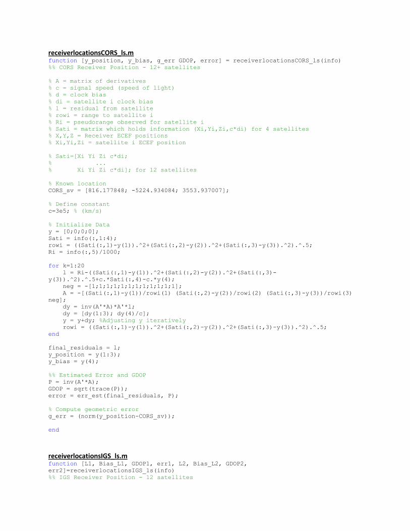
receiverlocationsCORS_ls.m function [y_position, y_bias, g_err GDOP, error] = receiverlocationsCORS_ls(info)

%% CORS Receiver Position - 12+ satellites



% d = clock bias








% Sati=[Xi Yi Zi c*di;

% ...

% Xi Yi Zi c*di]; for 12 satellites

% Known location

CORS_sv = [816.177848; -5224.934084; 3553.937007];

% Define constant

c=3e5; % (km/s)

% Initialize Data

y = [0;0;0;0];

Sati = info(:,1:4);


Ri = info(:,5)/1000;

for k=1:20

l = Ri-((Sati(:,1)-y(1)).^2+(Sati(:,2)-y(2)).^2+(Sati(:,3)-

y(3)).^2).^.5+c.*Sati(:,4)-c.*y(4);

neg = -[1;1;1;1;1;1;1;1;1;1;1;1];

A = -[(Sati(:,1)-y(1))/rowi(1) (Sati(:,2)-y(2))/rowi(2) (Sati(:,3)-y(3))/rowi(3)

neg];

dy = inv(A'*A)*A'*l;

dy = [dy(1:3); dy(4)/c];

y = y+dy; %Adjusting y iteratively


end

final_residuals = l;

y_position = y(1:3);

y_bias = y(4);

%% Estimated Error and GDOP

P = inv(A'*A);

GDOP = sqrt(trace(P));

error = err_est(final_residuals, P);

% Compute geometric error

g_err = (norm(y_position-CORS_sv));

end

receiverlocationsIGS_ls.m function [L1, Bias_L1, GDOP1, err1, L2, Bias_L2, GDOP2,

err2]=receiverlocationsIGS_ls(info)

%% IGS Receiver Position - 12 satellites



% d = clock bias








% Sati=[Xi Yi Zi c*di;

% ...

% Xi Yi Zi c*di]; for 12 satellites

% Define constant

c = 3e5; % (km/s)

% Initialize Data

y1 = [0;0;0;0];

y2 = [0;0;0;0];

Sati = info(:,1:4);

rowi1 = ((Sati(:,1)-y1(1)).^2+(Sati(:,2)-y1(2)).^2+(Sati(:,3)-y1(3)).^2).^.5;


Ri1 = info(:,6)/1000;

Ri2 = info(:,5)/1000;

% Iteratively solve for site vector using L1 data

for k=1:100

l1 = Ri1-((Sati(:,1)-y1(1)).^2+(Sati(:,2)-y1(2)).^2+(Sati(:,3)-

y1(3)).^2).^.5+c.*Sati(:,4)-c.*y1(4);

neg1 = -[1;1;1;1;1;1;1;1;1;1;1;1];

A1 = -[(Sati(:,1)-y1(1))/rowi1(1) (Sati(:,2)-y1(2))/rowi1(2) (Sati(:,3)-

y1(3))/rowi1(3) neg1];

dy1 = inv(A1'*A1)*A1'*l1;

dy1 = [dy1(1:3); dy1(4)/c];

y1 = y1+dy1;


end

% Iteratively solve for site vector using L2 data

for k=1:100

l2 = Ri2-((Sati(:,1)-y2(1)).^2+(Sati(:,2)-y2(2)).^2+(Sati(:,3)-

y2(3)).^2).^.5+c.*Sati(:,4)-c.*y2(4);

neg2 = -[1;1;1;1;1;1;1;1;1;1;1;1];

A2 = -[(Sati(:,1)-y2(1))/rowi2(1) (Sati(:,2)-y2(2))/rowi2(2) (Sati(:,3)-

y2(3))/rowi2(3) neg2];

dy2 = inv(A2'*A2)*A2'*l2;

dy2 = [dy2(1:3); dy2(4)/c];

y2 = y2+dy2;


end

final_residuals_L1 = l1;

final_residuals_L2 = l2;

Bias_L1 = y1(4);

Bias_L2 = y2(4);

L1 = y1(1:3);

L2 = y2(1:3);

%% Estimated Error and GDOP

P1 = inv(A1'*A1);

P2 = inv(A2'*A2);

GDOP1 = sqrt(trace(P1));

GDOP2 = sqrt(trace(P2));

err1 = err_est(final_residuals_L1, P1);

err2 = err_est(final_residuals_L2, P2);

end

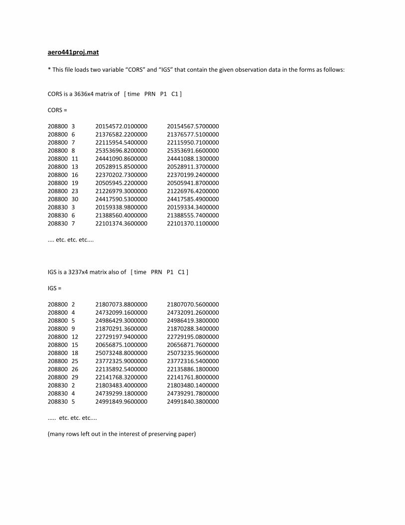
aero441proj.mat * This file loads two variable “CORS” and “IGS” that contain the given observation data in the forms as follows: CORS is a 3636x4 matrix of [ time PRN P1 C1 ] CORS = 208800 3 20154572.0100000 20154567.5700000 208800 6 21376582.2200000 21376577.5100000 208800 7 22115954.5400000 22115950.7100000 208800 8 25353696.8200000 25353691.6600000 208800 11 24441090.8600000 24441088.1300000 208800 13 20528915.8500000 20528911.3700000 208800 16 22370202.7300000 22370199.2400000 208800 19 20505945.2200000 20505941.8700000 208800 23 21226979.3000000 21226976.4200000 208800 30 24417590.5300000 24417585.4900000 208830 3 20159338.9800000 20159334.3400000 208830 6 21388560.4000000 21388555.7400000 208830 7 22101374.3600000 22101370.1100000 .... etc. etc. etc.... IGS is a 3237x4 matrix also of [ time PRN P1 C1 ] IGS = 208800 2 21807073.8800000 21807070.5600000 208800 4 24732099.1600000 24732091.2600000 208800 5 24986429.3000000 24986419.3800000 208800 9 21870291.3600000 21870288.3400000 208800 12 22729197.9400000 22729195.0800000 208800 15 20656875.1000000 20656871.7600000 208800 18 25073248.8000000 25073235.9600000 208800 25 23772325.9000000 23772316.5400000 208800 26 22135892.5400000 22135886.1800000 208800 29 22141768.3200000 22141761.8000000 208830 2 21803483.4000000 21803480.1400000 208830 4 24739299.1800000 24739291.7800000 208830 5 24991849.9600000 24991840.3800000 ..... etc. etc. etc.... (many rows left out in the interest of preserving paper)

gps group 9 project

Documents