gotthard-i documentation - psi.ch · gotthard-i documentation, release 0.2 to compile the software...

Gotthard-I DocumentationRelease 0.2

A. Mozzanica and J. Zhang

October 11, 2016

CONTENTS

1 Introduction to Gotthard-I 31.1 Introduction . . . . . . . . . . . . . . . . . . . . . . . . . . . . . . . . . . . . . . . . . . . . . . . 3

2 Softwares 52.1 The software package . . . . . . . . . . . . . . . . . . . . . . . . . . . . . . . . . . . . . . . . . . 52.2 Install softwares . . . . . . . . . . . . . . . . . . . . . . . . . . . . . . . . . . . . . . . . . . . . . 52.3 Upgrade softwares . . . . . . . . . . . . . . . . . . . . . . . . . . . . . . . . . . . . . . . . . . . . 8

3 Detector set-up and configuration 93.1 Connect the detector . . . . . . . . . . . . . . . . . . . . . . . . . . . . . . . . . . . . . . . . . . . 93.2 Configure the system . . . . . . . . . . . . . . . . . . . . . . . . . . . . . . . . . . . . . . . . . . . 103.3 Exit after measurements . . . . . . . . . . . . . . . . . . . . . . . . . . . . . . . . . . . . . . . . . 123.4 CLI mode . . . . . . . . . . . . . . . . . . . . . . . . . . . . . . . . . . . . . . . . . . . . . . . . . 123.5 Setup file . . . . . . . . . . . . . . . . . . . . . . . . . . . . . . . . . . . . . . . . . . . . . . . . . 173.6 Configure two detectors . . . . . . . . . . . . . . . . . . . . . . . . . . . . . . . . . . . . . . . . . 17

4 Use GUI to perform measurement 194.1 Usage of GUI . . . . . . . . . . . . . . . . . . . . . . . . . . . . . . . . . . . . . . . . . . . . . . . 194.2 Examples to set-up measurements . . . . . . . . . . . . . . . . . . . . . . . . . . . . . . . . . . . . 23

5 Characterization and calibration 255.1 Gains & offsets in “fixed” gain mode . . . . . . . . . . . . . . . . . . . . . . . . . . . . . . . . . . 255.2 Gains & offsets in dynamic gain mode . . . . . . . . . . . . . . . . . . . . . . . . . . . . . . . . . 265.3 Noise . . . . . . . . . . . . . . . . . . . . . . . . . . . . . . . . . . . . . . . . . . . . . . . . . . . 275.4 Energy conversion . . . . . . . . . . . . . . . . . . . . . . . . . . . . . . . . . . . . . . . . . . . . 28

6 Data processing 296.1 Data structure . . . . . . . . . . . . . . . . . . . . . . . . . . . . . . . . . . . . . . . . . . . . . . . 296.2 Conversion gain . . . . . . . . . . . . . . . . . . . . . . . . . . . . . . . . . . . . . . . . . . . . . 306.3 Pedestal and noise . . . . . . . . . . . . . . . . . . . . . . . . . . . . . . . . . . . . . . . . . . . . 326.4 Mask generation . . . . . . . . . . . . . . . . . . . . . . . . . . . . . . . . . . . . . . . . . . . . . 346.5 Energy conversion . . . . . . . . . . . . . . . . . . . . . . . . . . . . . . . . . . . . . . . . . . . . 356.6 Callables . . . . . . . . . . . . . . . . . . . . . . . . . . . . . . . . . . . . . . . . . . . . . . . . . 366.7 Last words . . . . . . . . . . . . . . . . . . . . . . . . . . . . . . . . . . . . . . . . . . . . . . . . 40

7 Routines 417.1 Python routines . . . . . . . . . . . . . . . . . . . . . . . . . . . . . . . . . . . . . . . . . . . . . . 41

8 Indices and tables 53

i

Gotthard-I Documentation, Release 0.2

This is a webpage documenting the Gotthard-I module information. For more details about the sen-sor, ASIC and readout of Gotthard-I, please refer to A. Mozzanica et al., JINST 7, C01019 (2012):http://iopscience.iop.org/article/10.1088/1748-0221/7/01/C01019.

This document gives a more practical information on the usage and characterization of the detector.

Document version: 0.2

Document contribution and revision:

A. Mozzanica (PSI), A. Parenti (XFEL.EU), D. Thattil (PSI), M. Turcato (XFEL.EU), J. Zhang (PSI)

Contents:

CONTENTS 1

http://iopscience.iop.org/article/10.1088/1748-0221/7/01/C01019


2 CONTENTS

CHAPTER

ONE

INTRODUCTION TO GOTTHARD-I

1.1 Introduction

Gotthard-I is a charge-integrating silicon micro-strip detector with a pitch of 50 um (or optionally 25 um), and 1280strips in total. It can be operated at < 1 MHz frame rate in burst mode. The schematic of Gotthard-I ASIC can be seenas below:

Gotthard-I has a dynamic gain switching pre-amplifier to achieve high dynamic range, and a CDS stage to removereset noise charge of the pre-amplifier. In dynamic gain switching mode, the CDS works before gain switching andis bypassed once gain switching happened. The detector can also work in a “fixed” gain mode, in which case only aconstant gain applies. In “fixed” gain mode, the feedback capacitance of the pre-amplifier is fixed according to theinput by users for detector operation, and the CDS stage is activated all the time.

In the following, the detailed information about how to configure and set-up the detector module, how to performmeasurements and get data, and how to perform data analysis with basic routines will be introduced.

3


4 Chapter 1. Introduction to Gotthard-I

CHAPTER

TWO

SOFTWARES

The SLS detectors software is intended to control the detectors developed by the SLS Detectors group. It provides acommand line interface (text client), a graphical user interface(GUI) as well as an API that can be embedded in youracquisitions system, some tools for detector calibration and the software to receive the data from detector with highdata throughput (e.g. Gotthard).

2.1 The software package

The SLS detector software (slsDetectorPackage) can be downloaded through: https://www.psi.ch/detectors/users-support. The complete software package is composed of several programs which can be installed (or locally compiled)depending on the needs:

• The slsDetector shared and static libraries which are necessary for all user interfaces.

• The command line interfaces which are provided to communicate with the detectors using the command lineand eventually to the data receiver

• The data receiver (slsReceiver), which can be run on a different machine, receives the data from the detector andinterfaces to the control software via TCP/IP for defining e.g. the file name, output path and return status andprogress of the acquisition

• The graphical user interface (slsDetectorGUI) which provides a user friendly way of operating the detectorswith online data preview

• The calibration wizards (energyCalibrationWizard, angularCalibrationWizard) to analyze the data and producethe energy or angular calibration files (only for photon-counting detector and thus not an interest for Gotthardusers)

• The Gotthard virtual servers to simulate the detectors behavior (however only control commands work, not thedata acquisition itself)

2.2 Install softwares

1. Prerequisites for using the softwares

The software is written in C/C++. It needs to be able to access the shared memeory of the control PC andcommunicate to the detectors over TCP/IP. Therefore the detector should receive a proper IP address (eitherDHCP or static) and no firewall should be present between th control PC and the detector.

For installing the slsDetector shared and static libraries and the slsDetectorClient software, any Linux installa-tion with a working gcc should be fine. The slsDetectorGUI is based on Qt4 with Qwt libraries. The calibrationwizards are based on the CERN Root data analysis framework.

5

https://www.psi.ch/detectors/users-support



To compile the software you will need the whole Qt4, Qwt and Root installation, including the header files. Torun the software, it is enough to have the Qt4, Qwt or Root libraries appended to the LD_LIBRARY_PATH.CERN Root is not mandatory if users perform data analysis with another program language.

For detector configuration and data acquisition, the minimal requirements can be summarized below:

• slsDetectorPackage: All detector related executables and libraries

• Qt-4.8.2, qwt-6.0.1 and Qwt3D: Necessary for the GUI

In addition to slsDetectorPackage, the Qt-4.8.2 software can be downloaded: ftp://ftp.qt.nokia.com/qt/source/qt-everywhere-opensource-src-4.8.1.tar.gz (or alternatively at http://doc.qt.io/qt-4.8), qwt-6.0.1:https://svn.code.sf.net/p/qwt/code/branches/qwt-6.0/, and Qwt3D: http://qwtplot3d.sourceforge.net/.

Installation of Qt-4.8.2:

> gunzip [qt_file_name].tar.gz> tar xvf [qt_file_name].tar> ./configure> make> make install

Installation of Qwt-related packages:

> svn co https://svn.code.sf.net/p/qwt/code/branches/qwt-6.0> cd qwt-6.0> qmake> make> make install

More information about the software installation can be found at the following link:https://www.psi.ch/detectors/UsersSupportEN/slsDetectorInstall.pdf

PS: If there are repositories including Qt-4.8.2 and Qwt existing, instead of using the fore-mentioned standardinstallation, simply try “yum install qt-devel qwt-devel root” for Scientific Linux, “apt-get install libqt4-devlibqwt4-dev root-system” for Ubuntu.

2. Export the libraries and executables through command line after software installation:

• Qt library:

> export QTDIR=[.../.../]Qt-4.8.2> export LD_LIBRARY_PATH=$QTDIR:$LD_LIBRARY_PATH> export PATH=$QTDIR/bin:$PATH

• g++ directory:

> export QMAKESPEC=$QTDIR/mkspecs/linux-g++

• qwt directory:

> export QWTDIR=[.../.../]qwt-6.0.1> export LD_LIBRARY_PATH=$QWTDIR:$LD_LIBRARY_PATH

• Qwt3D:

> export QWT3D=[.../]qwtplot3d> export LD_LIBRARY_PATH=$QWT3D:$LD_LIBRARY_PATH

It is also recommended to put them into the ”.bashrc” file so that they do not have to be input for each start.

3. Compile slsDetectorPackage

The slsReceiver and slsDetectorGui executables should be compiled before using:

6 Chapter 2. Softwares

ftp://ftp.qt.nokia.com/qt/source/qt-everywhere-opensource-src-4.8.1.tar.gz

ftp://ftp.qt.nokia.com/qt/source/qt-everywhere-opensource-src-4.8.1.tar.gz

http://doc.qt.io/qt-4.8

https://svn.code.sf.net/p/qwt/code/branches/qwt-6.0/

http://qwtplot3d.sourceforge.net/

https://www.psi.ch/detectors/UsersSupportEN/slsDetectorInstall.pdf


> cd [.../.../]slsDetectorPackage> make clean; make

Then export the libraries and executables:

> cd bin> export LD_LIBRARY_PATH=$PWD:$LD_LIBRARY_PATH> export PATH=$PWD:$PATH

The method mentioned above is the minimal effort to compile the slsDetectorPackage. Other compilation meth-ods:

• make -> compile the library, the command line interface and the receiver

• make lib -> compile only the library

• make slsDetectorClient -> compile the command line interface (and the library, since it is required)

• make slsDetectorClient_static -> static compile the command line interface statically linking the library(and the library, since it is required)

• make slsReceiver -> compile the data reciever (and the library, since it is required)

• make slsReceiver_static -> compile the data reciever statically linking the library (and the library, since itis required)

• make slsDetectorGUI -> compile slsDetectorGUI - requires a working Qt4 and Qwt installation

• make calWiz -> compile the calibration wizards - requires a working root installation

• make doc -> compile documentation in pdf format

• make htmldoc -> compile documentation in html format

• make install_lib -> installs the libraries, the text clients, the documentation and the includes for the API

• make install -> installs all software, including the gui, the cal wizards and the includes for the API

• make confinstall -> installs all software, including the gui, the cal wizards and the includes for the API,prompting for the install paths

• make clean -> remove object files and executables

• make help -> lists possible targets

• make gotthard_virtual -> compile a virtual GOTTHARD detector server (works for control commands,not for data taking)

The path where the files binaries, libraries, documentation and includes will be installed can either be definedinteractively by sourcing the configure script (not executing!) or during compilation using make confinstall ordefined on the command line deifning one (or all) the following variables (normally INSTALLROOT is enough):

• INSTALLROOT -> Directory where you want to install the software. Defaults to PWD

• BINDIR -> Directory where you want to install the binaries. Defaults to bin/

• INCDIR -> Directory where you want to pute the header files. Defaults to include

• LIBDIR -> Directory where you want to install the libraries. Defaults to bin/

• DOCDIR Directory where you want to copy the documentation. Defaults to doc/

To be able to run the executables, append the BINDIR directory to your PATH and LIBDIR to theLD_LIBRARY_PATH. To run the GUI, you also need to add to your LD_LIBRARY_PATH the Qt4 and Qwtlibraries, without the need to install the whole Qt and Qwt developer package:

• libqwt.so.6

2.2. Install softwares 7


• libQtGui.so.4

• libQtCore.so.4

• libQtSvg.so.4

More options and information about software installation can be found inhttps://www.psi.ch/detectors/UsersSupportEN/slsDetectorInstall.pdf.

2.3 Upgrade softwares

The softwares are released through the following webpage: https://www.psi.ch/detectors/users-support.It is recommended to check the new release there. The client, receiver and detector server have to beupdated at the same time. To update the detector server, follow the instruction below:

1. Server binary preparation

First, check the location of the tftp directory:

> more /etc/xinetd.d/tftp

The tftpboot directory will be shown after the “server_args”. Here in the test machine, it is “/tftp-boot”. If no tftp exists, download and install it: http://askubuntu.com/questions/201505/how-do-i-install-and-run-a-tftp-server.

The, copy the server binary to tftp directory:

> cp [.../.../]slsDetectorPackage/slsDetectorSoftware/gotthardDetectorServer/gotthardDetectorServer /tftpboot/

2. Update the detector server

After powering on the detector, do the following in the command line:

> telnet bchip050 (either the hostname or the IP address of the detector)> ps (list the running processes)> killall gotthardDetectorServer (stop the currently running server)> tftp -r pc_name gotthardDetectorServer -g> chmod 777 gotthardDetectorServer> ./gotthardDetectorServer & (start the new server)

Note that the bchip050 should be replaced by the hostname of the specific detector module.

8 Chapter 2. Softwares

https://www.psi.ch/detectors/UsersSupportEN/slsDetectorInstall.pdf


http://askubuntu.com/questions/201505/how-do-i-install-and-run-a-tftp-server

http://askubuntu.com/questions/201505/how-do-i-install-and-run-a-tftp-server

CHAPTER

THREE

DETECTOR SET-UP AND CONFIGURATION

The information about how to set-up the Gotthard-I detector and configure the detector has been summarized as below.

3.1 Connect the detector

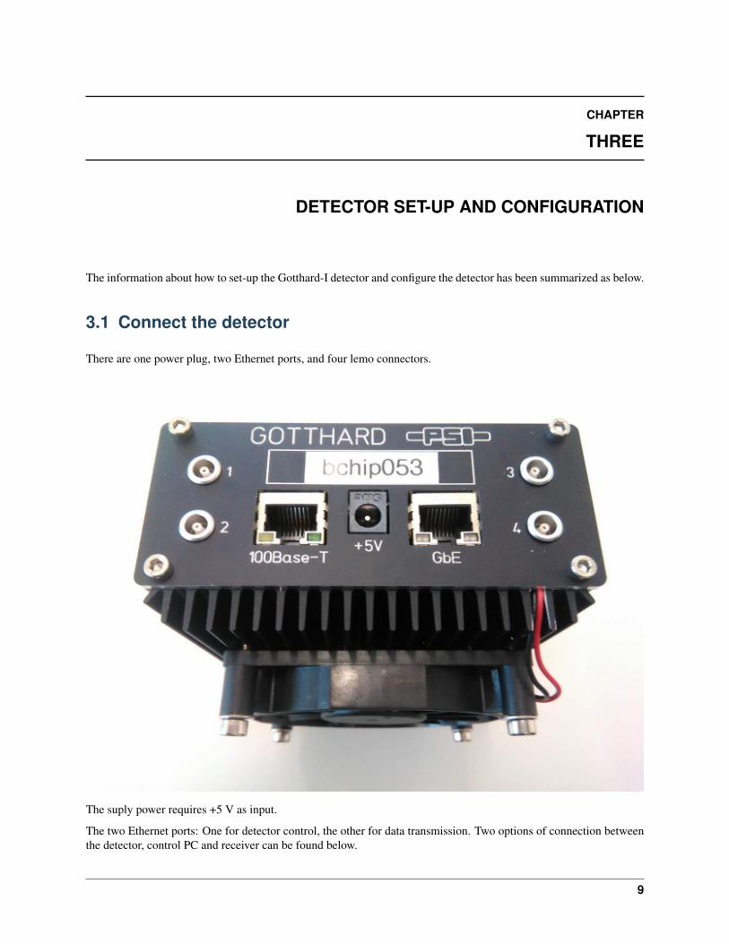
There are one power plug, two Ethernet ports, and four lemo connectors.

The suply power requires +5 V as input.

The two Ethernet ports: One for detector control, the other for data transmission. Two options of connection betweenthe detector, control PC and receiver can be found below.

9


The command can be sent through a control PC to the detector directly or through a receiver(refer to the figures above)and the data received by the receiver through 1 GbEthernet link under UDP protocal.

The four lemo connectors (labeled 1-4): 1 is used to receive triggers for the detector, 2-4 are triggers sent-out from thedetector. In order to trigger the detector by an external signal, refer to the section “Edit the configuration file”. Thelemo connectors 2-4 always generate trigger signals by the detector in case the other devices need to synchronize withit.

3.2 Configure the system

1. Edit the configuration file

The configuration file ends with an extension of ”.config”. In the whole text, the file name “bchip.config” isused.

1 type Gotthard+2 0:hostname 10.42.0.353 #0:port 19524 #0:stopport 19535 #0:rx_tcpport 19546 0:settingsdir /home/wp74diag/slsDetectorsPackage/settingsdir/gotthard7 0:angdir 1.0000008 0:moveflag 0.0000009 0:lock 0

10 0:caldir /home/wp74diag/slsDetectorsPackage/settingsdir/gotthard11 0:ffdir /home/wp74diag12 0:extsig:0 off

10 Chapter 3. Detector set-up and configuration


13 0:extsig:1 off14 0:extsig:2 off15 0:extsig:3 off16 0:detectorip 10.42.0.217 0:detectormac 00:aa:bb:cc:dd:ee18 0:rx_udpport 5000419 0:rx_hostname 10.42.0.120 0:outdir /home/wp74diag/data/gotthard21 0:vhighvoltage 12022 0:frames 100023 0:exptime 0.000124 0:period 0.010025 master -126 sync none27 outdir /home/wp74diag/data/gotthard28 ffdir /home/wp74diag29 headerbefore none30 headerafter none31 headerbeforepar none32 headerafterpar none33 badchannels none34 angconv none35 globaloff 0.00000036 binsize 0.00100037 threaded 1

The following line should be changed accordingly for each detector module or PC connection:

• L2: hostname or IP address for the detector

• L5: the communication port between client and receiver, 1954 by default

• L6 & L10: setting directory based on the location of slsDetectorsPackage folder

• L11, L20, L27 & L28: output directory of data

• L12: set to “trigger_in_rising_edge” if a trigger will be used. It is suggested to set it all the time. With this,it is also possible to work with “Auto” mode without triggers. The setting of different modes, e.g. “Auto”or “Trigger Exposure Series”, can be done from the “Timing Mode” box inside “Measurement” tab of theSLS Detector GUI. The details for setting GUI can be found in the Section “Usage of GUI” of Chapter“Use GUI to perform measurement”.

• L16: the ip address of the detector for the UPD interface with the receiver

• L17: the mac address of the detector upd interface to mac is configurable; any unique mac address can beset

• L18: the udp port of the receiver for data receiving

• L19: host name or IP address of the receiver for the TCP/IP interface with the client

• L21: bias voltage of the sensor; 200 V is recommended for operation

In addtion, the “rx_udpip” can also be set if several internet connections exist:

• rx_udpip: the ip address of the receiver for the UDP interface with the detector; it has to be on the sameinternet as L16

2. Power on the detector module first and start the detector server

The detector server will automatically start for users. If not, type the following in the command line:

3.2. Configure the system 11


> ping bchip050> telnet bchip050> killall gotthardDetectorServerroot:>./gotthardDetectorServer

Note that “bchip050” is the name of specific module! Try to ping the module and see whether it has beenconnected and then start the server.

3. Start receiver

To start the receiver on the PC, enter the “slsDetectorsPackage/bin” folder and type the following in the com-mand line:

> which slsReceiver (if path is configured correctly, it's in the right bin folder)> slsReceiver (Note: or ./slsReceiver)

The libSlsDetector.so and libSlsReceiver.so project libraries, and project executatbles should be added beforestarting receiver server. See chapter section-2.2.

4. Start GUI

To start GUI for detector control and data display, type the following in the command line:

> slsDetectorGui --f [.../.../]bchip.config

The -f option is only needed if the detector and receiver are not configured.

In the GUI pop-up, the “developer” tab will not be activated and thus the DAC values cannot be changed in theGUI (only in command line in this case). If a DAC value needs to be changed, the “developer” tab should beactivated and the following command should be used:

> slsDetectorGui -df [.../.../]bchip.config

In such case, the DAC values can be changed in-situ and the temperature of the FPGA can be readout. Only dothis if DAC values need to be changed.

Note that “export” has to be done to run any project executables.

3.3 Exit after measurements

1. Stop the receiver first:

> CTRL + C

2. Stop the detector server

This automatically done when powering off the detector.

3.4 CLI mode

The detector can also be ran and controlled without using GUI. In this case, the make file needs to be modified. Thisis useful if the QWT is not available on the system. To compile without GUI using: “make client; “make receiver;make” in the command line.

Some useful executables in such mode:



> sls_detector_put (Note: set a value of a parameter)> sls_detector_get (Note: get a value of a parameter)> sls_detector_help (Note: get help on something)> sls_detector_acquire (Note: acquire images)

The syntax of commands is:

> sls_detector_put [id]:command [argument] (for using sls detector class)> sls_detector_put [id]-command [arguments] (for using multi-detector class)

Initialization commands:

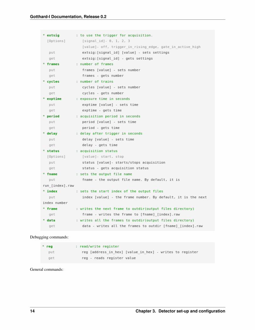
Acquisition commands:

3.4. CLI mode 13


Debugging commands:

General commands:



Commands for configuring network (these are normally not used independently, since a configuration file is loaded):

3.4. CLI mode 15


Example of using commands:



More useful commands can be found in https://www.psi.ch/detectors/UsersSupportEN/slsDetectorClientHowTo.pdf.

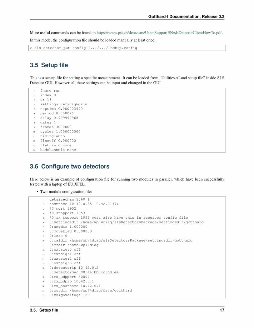
In this mode, the configuration file should be loaded manually at least once:

> sls_detector_put config [.../.../]bchip.config

3.5 Setup file

This is a set-up file for setting a specific measurement. It can be loaded from “Utilities->Load setup file” inside SLSDetector GUI. However, all these settings can be input and changed in the GUI.

1 fname run2 index 03 dr 164 settings veryhighgain5 exptime 0.0000029906 period 0.0000257 delay 0.9999999688 gates 19 frames 3000000

10 cycles 1.00000000011 timing auto12 fineoff 0.00000013 flatfield none14 badchannels none

3.6 Configure two detectors

Here below is an example of configuration file for running two modules in parallel, which have been successfullytested with a laptop of EU.XFEL.

• Two-module configuration file:

1 detsizechan 2560 12 hostname 10.42.0.35+10.42.0.37+3 #0:port 19524 #0:stopport 19535 #0:rx_tcpport 1956 must also have this in receiver config file6 0:settingsdir /home/wp74diag/slsDetectorsPackage/settingsdir/gotthard7 0:angdir 1.0000008 0:moveflag 0.0000009 0:lock 0

10 0:caldir /home/wp74diag/slsDetectorsPackage/settingsdir/gotthard11 0:ffdir /home/wp74diag12 0:extsig:0 off13 0:extsig:1 off14 0:extsig:2 off15 0:extsig:3 off16 0:detectorip 10.42.0.217 0:detectormac 00:aa:bb:cc:dd:ee18 0:rx_udpport 5000419 0:rx_udpip 10.42.0.120 0:rx_hostname 10.42.0.121 0:outdir /home/wp74diag/data/gotthard22 0:vhighvoltage 120

3.5. Setup file 17

https://www.psi.ch/detectors/UsersSupportEN/slsDetectorClientHowTo.pdf


23 0:frames 100024 0:exptime 0.000125 0:period 0.010026

27 #1:port 195228 #1:stopport 195329 #1:rx_tcpport 1956 must also have this in receiver config file30 1:settingsdir /home/wp74diag/slsDetectorsPackage/settingsdir/gotthard31 1:angdir 1.00000032 1:moveflag 0.00000033 1:lock 034 1:caldir /home/wp74diag/slsDetectorsPackage/settingsdir/gotthard35 1:ffdir /home/wp74diag36 1:extsig:0 off37 1:extsig:1 off38 1:extsig:2 off39 1:extsig:3 off40 1:rx_tcpport 172041 1:detectorip 10.42.0.342 1:detectormac 01:aa:bb:cc:dd:e143 1:rx_udpport 5000544 1:rx_udpip 10.42.0.145 1:rx_hostname 10.42.0.146 1:outdir /home/wp74diag/data/gotthard47 1:vhighvoltage 12048 1:frames 100049 1:exptime 0.000150 1:period 0.010051

52

53 master -154 sync none55 outdir /home/wp74diag/data/gotthard56 ffdir /home/wp74diag57 headerbefore none58 headerafter none59 headerbeforepar none60 headerafterpar none61 badchannels none62 angconv none63 globaloff 0.00000064 binsize 0.00100065 threaded 1


CHAPTER

FOUR

USE GUI TO PERFORM MEASUREMENT

4.1 Usage of GUI

As introduced in previous chapter, the GUI can be started with the following in the command line:

> slsDetectorGui --f [.../.../]bchip.config

The GUI includes several tabs for detector control and data acquisition.

• The “Measurement” tab:

In this tab, it is possible to specify the following parameters:

– Number of measurements: Each measurement includes a number of frames input on the right ofthe window

– Run index: The file name ends up with the index number, for example“run_f000000000000_RunIndex.raw”

19


– Number of frames: The total number of frames to be measured for each measurement

– Timing mode: “Auto” or “Trigger Exposure Series”. The former does not trigger whereas thelatter uses a trigger.

– Exposure time: Time of integration

– Acquisition period: Period per frame. The frame rate is given by 1 divided by the acquisitionperiod, for example 1 ms input gives a frame rate of 1 kHz.

– Number of triggers: Perform a number of frames for each trigger and total frames given bynumber of frames multiplying number of triggers for each measurement

– Delay after trigger: Delay time to start taking data after receiving a trigger signal

Note that in order to use the trigger mode, the line “0:extsig:0 off” in the configuration file has tobe changed to “0:extsig:0 trigger_in_rising_edge”. The #1 of the lemo connectors is used to receivetrigger signals. #2-4 are the trigger signals from the detector which can be used to synchronize theother devices when they need to be triggered by the detector, as explained in the previous chapter.

Only when the trigger mode is selected from the “Timing Mode” block, the input for “Number oftriggers” and “Delay after trigger” area can be activated.

• The “Setting” tab:

20 Chapter 4. Use GUI to perform measurement


– Settings: Select operating mode either “fixed” gain or dynamic gain switching

* High gain: Single photons regime low noise, working up to a few tens of 12 keV photons

* Very high gain: Single photons regime and very low noise, working up to a couple tens of12 keV photons

* Medium gain: No single photon sensitivity, working for photons between a few tens tohundreds

* Low gain: No single photon sensitivity, working for photons from a few hundreds to tenthousand

* Dynamic gain: Dynamically switch gain, working for single photon up to ten thousandphotons

• The “Data Output” tab: Choose the folder for output data

4.1. Usage of GUI 21


• The “Plot” tab:

The refresh rate of the plot in “Plotting window” can be set here. In addtion, pedestal subtracted



results can be shown in the “Plotting window” by perform an on-line pedestal subtration through“1D plot option 1” dialog.

• The other tabs:

Since the other tabs are irrelevant for users’ setting, they will not be discussed here.

4.2 Examples to set-up measurements

• Measurements without trigger:

– Choose “Auto” in “Timing Mode” of “Measurement” tab

– In “Settings”, select an operation gain in measurement: “Very High Gain”, “High Gain”, “Medium Gain”,“Low Gain”, or “Dynamic Gain”

– Enter the “Exposure Time” in “Measurement” tab: With “Very High Gain” and “High Gain” mode, the“Exposure Time” should not exceed a few tens of microsecond, otherwise the ADU saturates due to leakagecurrent.

– Enter the “Acquision Period” in “Measurement” tab: 100 microseciond or 1 milisecond and so on, depend-ing on the required frame rate.

– Set “Number of frames” in “Measurement” tab and “Number of Measurements”: The total frames givenby “Number of frames” multiplied by “Number of Measurements”.

– Set the “File Name” and “Run Index”

– Press the “Start” button in “Measurement” tab to start taking data

• Measurements with trigger:

– In the configuration file, change “0:extsig:0 off” to “0:extsig:0 trigger_in_rising_edge”; and then load theconfiguration file again from GUI: “Utilities” -> “Load Configuration File”

– Choose “Trigger Exposure Series” in “Timing Mode” of “Measurement” tab

– Input “Number of Triggers” to be received by the detector in the “Measurement” tab

– Input the delays through “Delay After Trigger” in the “Measurement” tab: The measurement starts withthis delay after receiving trigger signal

– In “Settings”, select an operation gain in measurement: “Very High Gain”, “High Gain”, “Medium Gain”,“Low Gain” or “Dynamic Gain”

– Enter the “Exposure Time” in “Measurement” tab: With “Very High Gain” and “High Gain” mode, the“Exposure Time” should not exceed a few tens of microsecond, otherwise the ADU saturates due to leakagecurrent.

– Enter the “Acquision Period” in “Measurement” tab: 100 microseciond or 1 milisecond and so on, depend-ing on the required frame rate.

– Set “Number of frames” in “Measurement” tab and “Number of Measurements”: The total frames givenby “Number of frames” multiplied by “Number of Measurements” and “Number of Triggers”

– Set the “File Name” and “Run Index”

– Press the “Start” button in “Measurement” tab to start taking data

• Note that the dark measurement, X-ray flurescence measurement with lab X-ray source can be done with “Auto”mode; whereas measurements with the single shot laser and synchrotron beam/FEL should be done with “Trig-ger” mode.

4.2. Examples to set-up measurements 23

CHAPTER

FIVE

CHARACTERIZATION AND CALIBRATION

To get correct photon energy from measurements with a charge-integrating detector (Gotthard), proper characterizationand calibration is necessary. This chapter will introduce the basic concept of detector calibration.

Usually, the following need to be characterized/calibrated:

• Gains and offsets in “fixed” gain mode (HG0, G0, G1 and G2)

• Gains and offsets in dynamic gain mode (G0, G1 and G2)

• Noise

The conversion of measured ADU to photon energy in a measurement will be based on the calibration results men-tioned above.

5.1 Gains & offsets in “fixed” gain mode

The gain and offset (also called “pedestal” sometimes) for very high gain (HG0) and high gain (G0) can be measuredwith X-ray fluorescence from an X-ray tube. However the gains for medium gain (G1) and low gain (G2) can only bemeasured with synchrotron/FEL beam instead of a lab X-ray source.

For example, in case a lab X-ray tube is used, the X-ray fluorescence from a Cu, Mo or other targets can be measuredusing Gotthard detector by putting it in front of the target. For this measurement, an exposure time (also called“integration time” sometimes) of a few microsecond, an acquisition period of 1 ms and “fixed” gain with either highgain (G0) or very high gain (HG0) shall be set. 2 us, 5 us and 10 us are commonly used as exposure time and >500000 frames recommended to obtain enough data.

After the measurement, the histogram/occurance of ADU values for each strip can be plotted and peak positions canbe extracted. As seen below, it is the histogram from a strip (Strip-64) in ameasurement using X-ray fluorescence froma Cu-target (Ka line at 8.05 keV). The 0, 1, ..., up to 4 photon peaks can be seen and their peak positions extracted andplotted as function of energy from different number of coincident photons.

25


The straight line fit gives the slope (gain in a unit of ADU/keV) and offset (in a unit of ADU). The gains for HG0 andG0 are different.

Since the medium gain and low gain are very small, it is not possible to get separated peak in the histogram usingX-ray fluorescence. In this case, multiple coincident photons from synchrotron/FEL beam should be used to calibrateG1 and G2.

The offsets (pedestals) for HG0, G0, G1 and G2 can be obtained from measurements using the same settings butwithout any X-rays. The mean or the center of a gaussian fit to the hitogram represents the offset (pedestal) for thespecific gain setting used in the measurement.

5.2 Gains & offsets in dynamic gain mode

In dynamic gain mode, the high gain (G0) is used as the initial gain stage. The gain [ADU/keV] and offset [ADU] ofhigh gain stage in dynamic gain mode are identical to the ones in “fixed” gain mode. That is, with X-ray fluorescence,the histogram for dynamic range mode and “fixed” gain mode using “high gain” are the same; however, the gainsand offsets of medium and low gains are different between dynamic gain mode and “fixed” gain mode. Thus, it isnecessary to calibrate the medium gain and low gain in dynamic range mode independent of the calibration of mediumgain and low gain in “fixed” gain mode. Similarly, these can be measured with either strong X-ray source (synchrotronor FEL) or laser.

For lab tests using a laser, one can select the dynamic gain in the setting. By scanning the laser intensity, it is possibleto obtain the dynamic range curve of a strip into which laser injects. The laser intensity can be converted to numberof photons or keV based on a conversion rate between the slope in high gain region and the high gain (G0) measuredwith X-ray fluorescence. The dynamic range curve from laser measurement is shown below:

26 Chapter 5. Characterization and calibration


Based on the fore-mentioned conversion, the medium and low gain region can be fit by staight lines separated and thengains and offsets extracted as indicated in the figure.

Note that all numbers indicate in the figures are from a prototype instead of a detector module and thus it can bedifferent from the results obtained with a detector module.

5.3 Noise

Noise is a key factor indicating the best separation of two different photon energies in a measurement. For example, fora noise of 300 e- (corresponding to 1 keV), a good energy separation can be achieved for 5 keV when counting 5 sigma.The noise is related to the exposure time and temperature. For a “fixed” experimental condition where exposure timeand temperature do not change, the noise can also be measured through “dark” measurement: Operating the detectorin a light-tight environment without X-rays. The settings for exposure time and acquisition period can be identical tothe ones in X-ray measurement but not mandatory. The number of frames can be less, for example ~ 10 000 frames intotal.

After the measurement, the histogram/occurance of ADU values for each strip shall be calculated. The distributionof histogram is fited by a gaussian function with mean value the offset (pedestal) as mentioned before and the sigma(unit: ADU) the noise related parameter. Then the noise can be calculated based on the following formula:

Noise[E.N.C.]=Sigmal[ADU]/gain[ADU/keV]*1000/3.6[eV]

Here below is an example of noise measurement with very high gain and high gain:

5.3. Noise 27


It is recommended to perform this measurement with the same settings used for an experiment.

5.4 Energy conversion

Once the gains and offsets calibrated, the conversion can be done with:

photon_energy=(Analog[ADU]-offset[ADU])/gain[ADU/keV]

using offset (pedestal) and gain values for specific gain stages.

28 Chapter 5. Characterization and calibration

CHAPTER

SIX

DATA PROCESSING

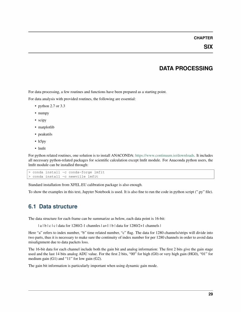
For data processing, a few routines and functions have been prepared as a starting point.

For data analysis with provided routines, the following are essential:

• python 2.7 or 3.3

• numpy

• scipy

• matplotlib

• peakutils

• h5py

• lmfit

For python related routines, one solution is to install ANACONDA: https://www.continuum.io/downloads. It includesall necessary python-related packages for scientific calculation except lmfit module. For Anaconda python users, thelmfit module can be installed through:

> conda install -c conda-forge lmfit> conda install -c newville lmfit

Standard installation from XFEL.EU calibration package is also enough.

To show the examples in this text, Jupyter Notebook is used. It is also fine to run the code in python script (”.py” file).

6.1 Data structure

The data structure for each frame can be summarize as below, each data point is 16-bit:

| a | b | c | c | data for 1280/2-1 channles | a+1 | b | data for 1280/2+1 channels |

Here “a” refers to index number, “b” time related number, “c” flag. The data for 1280 channels/strips will divide intotwo parts, thus it is necessary to make sure the continuity of index number for per 1280 channels in order to avoid datamisalignment due to data packets loss.

The 16-bit data for each channel include both the gain bit and analog information: The first 2 bits give the gain stageused and the last 14 bits analog ADU value. For the first 2 bits, “00” for high (G0) or very high gain (HG0), “01” formedium gain (G1) and “11” for low gain (G2).

The gain bit information is particularly important when using dynamic gain mode.

29

https://www.continuum.io/downloads


6.2 Conversion gain

The gain for very high gain (HG0) and high gain (G0) can be calculated based on X-ray fluorescence data withthe function: calGain_Xray(Folder, Run_index, binsize=5, E_xray=8.05, half_region=10, thres=0.2, min_dist=40,channels=linspace(1,1280,1280), common_correction=”No”). The input parameters are:

• Folder: where the data file located

• Run_index: the input index number in GUI. This number is in front of ”.raw” in the name of measurement files.

• binsize: the bin size to generate the histogram

• E_xray: energy of the X-ray fluorescence

• half_region: half of the fitting region per peak

• thres: threshold to consider as a peak in its histogram

• min_dist: minimal distance between two peaks

• channels: input channels to be calcuated

• common_correction: whether a common mode correction is mode or not

It calls function index_peaks() using “thres” and “min_dist” as input defined in PeakUtils module. More informationabout this module can be found at http://pythonhosted.org/PeakUtils/.

Below is an example about how to use the function calGain_Xray(). Download the example athttps://desycloud.desy.de/index.php/s/E2n1uRYXogabLhA.

30 Chapter 6. Data processing

http://pythonhosted.org/PeakUtils/

https://desycloud.desy.de/index.php/s/E2n1uRYXogabLhA


6.2. Conversion gain 31


Another function can also be called for gain calculation using lmfit module with a method of multi-peak fitting:calGain_Xray_lmfit(Folder, Run_index, binsize=5, Exray=8.05, gain_guess=10.0, sigma_guess=15, prob_1ph=0.4,channels=linspace(1,1280,1280), common_correction=”No”). The input parameters are:



• binsize: the bin size to generate the histogram

• E_xray: energy of the X-ray fluorescence

• gain_guess: initial guess of gain value in terms of ADU/keV

• sigma_guess: initial guess of sigma value of gaussian fitting to noise and single photon peak

• prob_1ph: initial guess of single photon probability per channel per frame

• channels: input channels to be calcuated

• common_correction: whether a common correction is mode or not

It is recommended to run both functions separately and merge the gain data, especially for the channels with failedfitting. If the convergence is not good enough, the program should run a few times till satisfication reached. Theexample for gain data merging can be downloaded at https://desycloud.desy.de/index.php/s/vBIZ2hZqkKHVksP.

6.3 Pedestal and noise

The pedestal (offset) and noise can be calculated for dark measurement in a light-tight box with the function: cal-Noise_ADU(Folder, Run_index, binsize=5, common_correction=”No”). The input parameters are:




https://desycloud.desy.de/index.php/s/vBIZ2hZqkKHVksP


• binsize: the bin size to fill in the histogram

• common_correction: whether a common correction is mode or not

The calculated noise in terms of ADU can be converted to equivalent noise charge (E.N.C.) with the function convert-Noise(noise_ADU, gain). The input:

• noise_ADU: the output from calNoise_ADU() function

• gain: the output from calGain_Xray() function

Below is an example about how to use the function calNoise_ADU() and convertNoise(). Download the example athttps://desycloud.desy.de/index.php/s/T2XCi9orhNv1MDl.

6.3. Pedestal and noise 33

https://desycloud.desy.de/index.php/s/T2XCi9orhNv1MDl


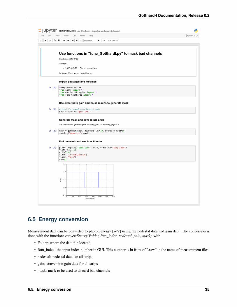
6.4 Mask generation

For dead channels and noisy channels, it is possible to generate a mask which can be used to mask out the bad datawhen converting measurement to photon energy. The function for generating mask: genMask(data, boundary_low,boundary_high), with

• data: either gain result or noise result

• boundary_low: channel with data below this boundary to be considered as a bad channel to be masked

• boundary_high: channel with data above this boundary to be considered as a bad channel to be masked

Below is an example about how to use the function genMask(). Download the example athttps://desycloud.desy.de/index.php/s/gVJQ49QinjpXf0Q.


https://desycloud.desy.de/index.php/s/gVJQ49QinjpXf0Q


6.5 Energy conversion

Measurement data can be converted to photon energy [keV] using the pedestal data and gain data. The conversion isdone with the function: convertEnergy(Folder, Run_index, pedestal, gain, mask), with



• pedestal: pedestal data for all strips

• gain: conversion gain data for all strips

• mask: mask to be used to discard bad channels

6.5. Energy conversion 35


By applying this function, a series of files in hdf5 format named “convertEnergy_XXX.nxs” will be generated, eachmax.20 GB with converted photon energy saved. The saved file with photon energy can be open with hdfview.

Below is an example about how to use the function convertEnergy(). Download the example athttps://desycloud.desy.de/index.php/s/hss5kkxhtHN9JO8.

6.6 Callables

Here below will list the functions written in python, which can be called directly after importing the“func_GotthardI.py” module.

• getHist(Folder, Run_index, i_strip, binsize, common_correction)

– This function will return the histogram for a specific strip.

– Input:


https://desycloud.desy.de/index.php/s/hss5kkxhtHN9JO8


* Folder: where the data file located

* Run_index: the input index number in GUI. This number is in front of ”.raw” in the name of mea-surement files

* i_strip: get the histogram for which strip

* binsize: bin size in terms of ADU to get the histogram

* common_correction: whether a common mode correction is preferred

– Return:

* bins

* occurance

• plotHist(Folder, Run_index, i_strip, binsize, common_correction)

– This function will run getHist first and plot the histogram

– Input:



* i_strip: get the histogram for which strip


* common_correction: whether a common correction is preferred

– Return:

* bins

* occurance

• getGain_Xray(bins, occurance, E_xray, half_region, thres, min_dist)

– This function will calculate the gain according to the input histogram and energy of X-ray

– Input:

* bins: the bins from output of getHist() or plotHist()

* occurance: the occurance for each bin from the output of getHist() or plotHist()

* E_xray: energy of X-ray characteristic line

* half_region: half of peak region to be fit with Gaussian

* thres: the threshold counts as a peak

* min_dist: minimal distance between two peaks

– Return:

* gain: calculated gain from the input histogram

* offset: offset/pedestal of the histogram

* gain_error: error of calculated gain

* peak_pos: the peak positions

* E_peaks: the corresponding peak energies

• getGain_Xray_lmfit(bins, occurance, Exray, gain_guess, sigma_guess, prob_1ph)

6.6. Callables 37


– This function will calculate the gain according to the input histogram and energy of X-ray using lmfitmodule

– Input:



* Exray: energy of X-ray characteristic line

* gain_guess: initial guess of conversion gain

* sigma_guess: initial guess of sigma for a gaussian fitting

* prob_1ph: probability of seeing 1 photon per channel per frame

– Return:

* gain: calculated gain from the input histogram

* offset: offset/pedestal of the histogram

* gain_error: error of calculated gain, 0 given at the moment

* peak_pos: the peak positions

* E_peaks: the corresponding peak energies

• calGain_Xray(Folder, Run_index, binsize, E_xray, half_region, thres, min_dist, common_correction)

– This function will calculate the gains for all strips/channels

– Input:


* Run_index: the input index number in GUI. This number is in front of ”.raw” in the name of mea-surement files.

* binsize: the bin size to generate the histogram

* E_xray: energy of the X-ray fluorescence

* half_region: half of the fitting region per peak

* thres: threshold to consider as a peak in its histogram

* min_dist: minimal distance between two peaks


– Return:

* gain: calculated gain for all strips

* offset: offset/pedestal for all strips

* gain_error: error of gain for each strip

• calGain_Xray_lmfit(Folder, Run_index, binsize, Exray, gain_guess, sigma_guess, prob_1ph, com-mon_correction)

– This function will calculate the gains for all strips/channels based on lmfit module

– Input:





* binsize: the bin size to generate the histogram

* Exray: energy of X-ray characteristic line

* gain_guess: initial guess of conversion gain

* sigma_guess: initial guess of sigma for a gaussian fitting

* prob_1ph: probability of seeing 1 photon per channel per frame


– Return:

* gain: calculated gain for all strips

* offset: offset/pedestal for all strips

* gain_error: error of gain for each strip

• getNoise_ADU(bins, occurance)

– This function will calculate the noise in terms of ADU for a specific input histogram

– Input:



– Return:

* sigma: the noise in terms of ADU

* pedestal: offset/pedestal from the noise measurement

* sigma_error: error of noise in terms of ADU

* pedestal_error: error of offset/pedestal

• calNoise_ADU(Folder, Run_index, binsize, common_correction)

– This function will calculate the noise in ADU for all strips

– Input:





– Return:

* sigma: the noise in terms of ADU

* pedestal: offset/pedestal from the noise measurement

* sigma_error: error of noise in terms of ADU

* pedestal_error: error of offset/pedestal

• convertNoise(noise_ADU, gain)

– This function will convert the noise in ADU to equivalent electron charge (E.N.C.)

6.6. Callables 39


– Input:

* noise_ADU: the calculated noise in [ADU]

* gain: the calculated gain in [ADU/keV]

– Return:

* noise_e: noise E.N.C. [e-]

• genMask(data, boundary_low, boundary_high)

– This function will generate a mask according to input data and boundaries

– Input:

* data: either gain or noise

* boundary_low: the low boundary for reliable data

* boundary_high: the high boundary for reliable data

– Return:

* mask: the mask for strips. 1 -> good strip/channel, 0 -> masked strip/channel

• convertEnergy(Folder, Run_index, pedestal, gain, mask)

– This function will convert the measurement into photon energy and save the data into a file with hdf format

– Input:



* pedestal: pedestal data for all strips

* gain: conversion gain data for all strips

* mask: mask to be used to discard bad channels

– Return:

* No data return but all saved into a hdf file automatically

6.7 Last words

All routines and functions provided are only served as a basis for understanding the data process and analysis. Thechoise of programming language and software is up to the users.


CHAPTER

SEVEN

ROUTINES

7.1 Python routines

There is a python module called “func_GotthardI.py”, in which the basic functions are defined and can be called byimporting this module. The file can be downloaded at https://desycloud.desy.de/index.php/s/VbhSuBmlIM18GHx.

1 """2 # A collection of functions for Gotthard-I module3 Changes:4 - 2016-08-09 Common mode correction with Gaussian fit to get the mean value per frame5 - 2016-08-05 Add common mode correction for function getHist() and plotHist() and calNoise_ADU()6 - 2016-08-05 Add functions calGain_Xray_lmfit() and getGain_Xray_lmfit() using lmfit module for gain calculation as an option and compensation for mis-calculation by calGain_Xray() and getGain_Xray()7 - 2016-08-04 Add error handling for function calNoise_ADU()8 - 2016-08-03 Solve the run_index non-umbiguous problem for function getHist() and convertEnergy()9 - 2016-08-03 Merge with the modification by Andrea

10 - 2016-08-03 Correct the threshold input error for function index_peaks()11 - 2016-07-28 Change the way of file sorting12 - 2016-07-25 Decode gain bit in fixed gain mode for functions: getHist() and convertEnergy()13 - 2016-07-21 First creation14

15 # Created by [email protected] """17

18 #!/usr/bin/env python19 # ld elements in base 2, 10, 16.20

21 import os,sys22 from numpy import *23 from matplotlib.pyplot import *24 from pylab import *25 from scipy.optimize import curve_fit26 import peakutils27 from lmfit.models import GaussianModel, ExponentialModel28 from lmfit import minimize, Minimizer, Parameters, Parameter, report_fit29

30

31

32 ############### FUNCTION COLLECTIONS FOR DATA CONVERSION ###############33 # global definition34 # base = [0, 1, 2, 3, 4, 5, 6, 7, 8, 9, A, B, C, D, E, F]35 base = [str(x) for x in range(10)] + [ chr(x) for x in range(ord('A'),ord('A')+6)]36

37 # bin2dec38 def bin2dec(string_num):39 return str(int(string_num, 2))

41

https://desycloud.desy.de/index.php/s/VbhSuBmlIM18GHx


40

41 # hex2dec42 def hex2dec(string_num):43 return str(int(string_num.upper(), 16))44

45 # dec2bin46 def dec2bin(string_num):47 num = int(string_num)48 mid = []49 while True:50 if num == 0: break51 num,rem = divmod(num, 2)52 mid.append(base[rem])53

54 return ''.join([str(x) for x in mid[::-1]])55

56 # dec2hex57 def dec2hex(string_num):58 num = int(string_num)59 mid = []60 while True:61 if num == 0: break62 num,rem = divmod(num, 16)63 mid.append(base[rem])64

65 return ''.join([str(x) for x in mid[::-1]])66

67 # hex2tobin68 def hex2bin(string_num):69 return dec2bin(hex2dec(string_num.upper()))70

71 # bin2hex72 def bin2hex(string_num):73 return dec2hex(bin2dec(string_num))74 ########################################################################75

76

77

78 ################### DEFINE FUNCTIONS FOR FITTING #######################79 # Define fitting functions80 # Gaussian81 def func_gauss(x, A, xbar, sigma):82 return A*exp(-(x-xbar)**2/(2*sigma**2))83 # Linear84 def func_lin(x, k, b):85 return k*x+b86

87 # Sqrt88 def func_sqrt(x, k, b):89 return k*sqrt(x)+b90

91 # Sqrt all component92 def func_sqrt_all(x, k, b):93 return sqrt(k*x+b)94

95 # Log1096 def func_log10(x, k, b):97 return k*log10(x+1)+b

42 Chapter 7. Routines


98

99 # Linear + exponential100 def func_lin_exp(x, k, b, A, tau):101 return k*x+b-A*exp(-x/tau)102

103 # Pure exponential104 def func_exp_pure(x, A, tau):105 return A*exp(-x/tau)106

107 # Exponential with shift108 def func_exp_shift(x, A, tau, xbar):109 return A*exp((x-xbar)/tau)110 ########################################################################111

112

113 ############################## Histogram related #######################114 # Plot the distribution of ADU in histogram115 def plot_histogram(data_array, binsize=5, style="-", label=""):116 """117 # Use hist from matplotlib function118 n, bins, patches = hist(data_array, bins=16385/binsize, range=(0,16385), histtype="step", align = "mid")119 print(len(n), len(bins))120 """121 # Use histogram from numpy function122 range_ADU = linspace(0, 16385, 16386)123 bins = range_ADU[0::binsize]124 occurance = histogram(data_array, bins)[0]125 plot(bins[1:], occurance, style, label=label, drawstyle="steps-mid", linewidth=2.0)126 legend(loc=1, frameon=False, fontsize=10)127 grid(True)128 xlim(0,16000)129 xlabel("ADU")130 ylabel("Occurance")131 return bins[1:], occurance, std(data_array), mean(data_array)132

133 # Generate the histogram for input data array134 def histogram_array(data_array, binsize=5):135 range_ADU = linspace(0, 16385, 16386)136 bins = range_ADU[0::binsize]137 occurance = histogram(data_array, bins)[0]138 return bins[1:], occurance139

140 # Generate the histogram for input data array141 def histogram_array_ADC(data_array, nbits=12, binsize=5):142 range_ADU = linspace(0, 2**nbits, 2**nbits+1)-binsize/2.0143 bins = range_ADU[0::binsize]144 occurance = histogram(data_array, bins)[0]145 return bins[1:], occurance146

147 # Generate the histogram for input data array148 def histogram_array_range(data_array, bins):149 occurance = histogram(data_array, bins)[0]150 return bins[1:], occurance151 ########################################################################152

153

154

155 ######################## Fitting related func ############################

7.1. Python routines 43


156 # Get mean and sigma from a gaussian fitting157 def para_gauss_fit(xdata, ydata, p0, thr=0):158 ydata_thr = ydata[where(ydata>=thr)[0]]159 xdata_thr = xdata[where(ydata>=thr)[0]]160 if len(ydata_thr) > 1:161 try:162 popt, pcov = curve_fit(func_gauss, xdata_thr, ydata_thr, p0=p0)163 except RuntimeError:164 popt = zeros(3, dtype="uint32")165 popt[0] = max(ydata_thr)166 popt[1] = xdata_thr[where(ydata_thr==max(ydata_thr))[0]]167 popt[2] = 0168 pcov = zeros((3,3))169 return popt, pcov170 else:171 popt = ydata_thr[0], xdata_thr[0], 0172 #popt = 0, 0, 0173 pcov = zeros((3,3))174 return popt, pcov175

176 # Get mean and sigma from a gaussian fitting, the curve_fit function with errors input for data177 def para_gauss_fit_error_in(xdata, ydata, p0, thr=0, sigma=None, absolute_sigma=False):178 ydata_thr = ydata[where(ydata>=thr)[0]]179 xdata_thr = xdata[where(ydata>=thr)[0]]180 if len(ydata_thr) > 1:181 try:182 popt, pcov = curve_fit(func_gauss, xdata_thr, ydata_thr, p0=p0, sigma=sigma, absolute_sigma=absolute_sigma)183 except RuntimeError:184 popt = zeros(3, dtype="uint32")185 popt[0] = max(ydata_thr)186 if len(where(ydata_thr==max(ydata_thr))[0])==1:187 popt[1] = xdata_thr[where(ydata_thr==max(ydata_thr))[0]]188 else:189 popt[1] = xdata_thr[where(ydata_thr==max(ydata_thr))[0][0]]190 popt[2] = 0191 pcov = zeros((3,3))192 return popt, pcov193 else:194 popt = ydata_thr[0], xdata_thr[0], 0195 pcov = zeros((3,3))196 return popt, pcov197

198 # Get parameters from a linear fit, the curve_fit function with errors input for data199 def para_lin_fit_error_in(xdata, ydata, p0, sigma=None, absolute_sigma=False):200 if len(ydata) > 1:201 try:202 popt, pcov = curve_fit(func_lin, xdata, ydata, p0=p0, sigma=sigma, absolute_sigma=absolute_sigma)203 except RuntimeError:204 popt = zeros(2)205 pcov = zeros((2,2))206 return popt, pcov207 else:208 popt = zeros(2)209 pcov = zeros((2,2))210 return popt, pcov211

212

213 # Peak indexes of distributions using peakutils packages



214 # Input: thres - in percentage of peak value215 # min_dist - in difference of index numbers216 def index_peaks(data_array, thres=0.01, min_dist=40):217 return peakutils.indexes(data_array, thres=thres, min_dist=min_dist)218

219

220 # Moving average221 def moving_average(a, n=2) :222 ret = cumsum(a, dtype=float)223 ret[n:] = ret[n:] - ret[:-n]224 return ret[n - 1:] / n225

226

227 # Moving sum228 def moving_sum(a, n=2) :229 ret = cumsum(a, dtype=float)230 ret[n:] = ret[n:] - ret[:-n]231 return ret[n - 1:]232 ########################################################################233

234

235 ######################## High level functions ##########################236 # Get histogram from X-ray measurement237 def getHist(Folder, Run_index, i_strip=500, binsize=5, common_correction="No"):238

239 # Get all files with this index240 files = []241 files += [each for each in os.listdir(Folder) if each.endswith("_"+str(Run_index)+'.raw')]242 # Sort files by generation time243 #files.sort(key=lambda x: os.path.getmtime(x)) # Opt-1244 files.sort() # Opt-2245 #print(files)246

247 N_channels = 1280 # Number of channels248 Header = 6 # x 16 bits (2 bytes)249 Header_odd = 4250 Header_even = 2251

252 Frame_length = Header + N_channels253 Frame_halflength = int(Frame_length/2)254

255 # loop all files256 for i in range(len(files)):257 #print("It is processing", i+1, "th file...")258 Filepath = Folder + files[i]259

260 Data = fromfile(Filepath, dtype=uint16, count=-1)261

262 nPackets = len(Data)/Frame_halflength263 #print("The number of packets received:", nPackets)264 #print(Data[:Frame_halflength])265 #print(Data[Frame_halflength:2*Frame_halflength])266

267 # Index of packets268 Index_packets = Data[0::Frame_halflength]269 #print(Index_packets)270

271 # Index for odd and even number of indexes



272 Index_packets_odd = where(mod(Index_packets,2)==1)[0]273 Index_packets_even = where(mod(Index_packets,2)==0)[0]274 #print(Index_packets_odd, Index_packets_even)275

276 # Give a specific strip277 if i_strip <= N_channels/2 - 2 + 1: # data in odd number of index278 Data_i_strip_file = Data[Index_packets_odd*Frame_halflength+i_strip+Header_odd-1]279 else: # data in even number of index280 Data_i_strip_file = Data[Index_packets_even*Frame_halflength+i_strip-int(N_channels/2-2)+Header_even-1-1]281

282 # Get rid of the gain bit of data283 Data_i_strip_file[where(Data_i_strip_file<2**14)[0]] = Data_i_strip_file[where(Data_i_strip_file<2**14)[0]]284 Data_i_strip_file[concatenate((where(Data_i_strip_file>=2**14)[0], where(Data_i_strip_file<2**15+2**14)[0]))] = Data_i_strip_file[concatenate((where(Data_i_strip_file>=2**14)[0], where(Data_i_strip_file<2**15+2**14)[0]))] - 2**14285 Data_i_strip_file[where(Data_i_strip_file>=2**15+2**14)[0]] = Data_i_strip_file[where(Data_i_strip_file>=2**15+2**14)[0]] - (2**15+2**14)286

287 # Accumulate the data for each file288 #Data_i_strip.append(Data_i_strip_file)289 #print(i, len(files))290

291 # Check whether the common mode correction is on or not292 if common_correction == "No":293 Data_i_strip_file = Data_i_strip_file294 elif common_correction == "Yes":295 if len(Index_packets_odd) != len(Index_packets_even):296 print("Packets lost! Watch out the correctness of the common mode correction!")297

298 CM_corr = []299 for iPacket in range(len(Index_packets_odd)):300 data_1Packet = Data[Index_packets_odd[iPacket]*Frame_halflength+Header_odd:Index_packets_odd[iPacket]*Frame_halflength+Header_odd+int(N_channels/2-1)]301 data_2Packet = Data[Index_packets_even[iPacket]*Frame_halflength+Header_even:Index_packets_even[iPacket]*Frame_halflength+Header_even+int(N_channels/2+1)]302 data_frame = concatenate((data_1Packet, data_2Packet))303

304 # Opt-1: Use a mean value of each frame to make common correction305 CM_corr = append(CM_corr, mean(data_frame))306 """307 # Opt-2: Use a gaussian fitting to get the mean of gaussian308 bins_frame, occurance_frame = histogram_array(data_frame, binsize=binsize)309 sigma_frame, pedestal_frame, sigma_error_frame, pedestal_error_frame = getNoise_ADU(bins_frame, occurance_frame)310 CM_corr = append(CM_corr, pedestal_frame)311 """312

313 # Take the first frame as reference314 if len(CM_corr) != 0:315 CM_corr = CM_corr - CM_corr[0]316 Data_i_strip_file = Data_i_strip_file - CM_corr317 else:318 print("The input for common_correction should be either Yes or No.")319

320 # Accumulate the accurrance321 bins, occurance_file = histogram_array(Data_i_strip_file, binsize=binsize)322 if i == 0:323 occurance = occurance_file324 else:325 occurance = occurance + occurance_file326

327 return bins, occurance328

329



330 # Plot the histogram from Xray331 def plotHist(Folder, Run_index, i_strip=500, binsize=5, common_correction="No"):332

333 bins, occurance = getHist(Folder, Run_index, i_strip=i_strip, binsize=binsize, common_correction=common_correction)334

335 # plot it336 figure("histogram")337 plot(bins, occurance, drawstyle="steps-pre", linewidth=1.0)338 grid(True)339 #xlim(0,16000)340 xlim(bins[where(occurance>1)[0]].min(), bins[where(occurance>1)[0]].max())341 ylim(1,)342 yscale("log")343 xlabel("ADU")344 ylabel("Occurance")345 show()346

347 return bins, occurance348

349

350 # Calculate gain from X-ray fluorescence measurement using peakutils and curve_fit of scipy351 def getGain_Xray(bins, occurance, E_xray=8.05, half_region=10, thres=0.2, min_dist=40):352

353 # Do peak finding and linear fitting here354 # Peak finding355 peak_index_guess = index_peaks(where(occurance>1, occurance, 1), thres=thres, min_dist=min_dist)356 #print("The index of peak position:", peak_index_guess)357 n_peaks = len(peak_index_guess)358

359 if n_peaks!= 0:360 E_peaks = linspace(0, n_peaks-1, n_peaks)*E_xray361 E_plot = linspace(-1, n_peaks, 100)*E_xray # Generate a series energy points for plotting362 peak_pos_i_strip = zeros(n_peaks)363 peak_pos_error_i_strip = zeros(n_peaks)364 # Peak fitting365 for i in range(n_peaks):366 popt, pcov = para_gauss_fit_error_in(bins[peak_index_guess[i]-half_region:peak_index_guess[i]+half_region], occurance[peak_index_guess[i]-half_region:peak_index_guess[i]+half_region], p0=[occurance[peak_index_guess[i]], bins[peak_index_guess[i]], 20.0], thr=thres, sigma=sqrt(occurance[peak_index_guess[i]-half_region:peak_index_guess[i]+half_region]), absolute_sigma=True)367 #popt, pcov = para_gauss_fit_error_in(bins[peak_index_guess[i]-half_region:peak_index_guess[i]+half_region], occurance_i_strip[peak_index_guess[i]-half_region:peak_index_guess[i]+half_region], p0=[occurance_i_strip[peak_index_guess[i]], bins[peak_index_guess[i]], 20.0], thr=0)368 peak_pos_i_strip[i] = popt[1]369 peak_pos_error_i_strip[i] = sqrt(pcov[1][1])370

371

372 # Calculate gain for the input strip from one ADC373 popt, pcov = para_lin_fit_error_in(E_peaks, peak_pos_i_strip, p0=[35.0, peak_pos_i_strip[0]], sigma=peak_pos_error_i_strip, absolute_sigma=True)374 gain_i_strip = popt[0]375 offset_i_strip = popt[1]376 gain_error_i_strip = sqrt(pcov[0][0])377

378 return gain_i_strip, offset_i_strip, gain_error_i_strip, peak_pos_i_strip, E_peaks379

380 else: # For the channel dead381 print("No proper value find by peakutils! A dead channel?")382 gain_i_strip = 0383 offset_i_strip = 0384 gain_error_i_strip = 0385 peak_pos_i_strip = 0386 E_peaks = 0387



388 return gain_i_strip, offset_i_strip, gain_error_i_strip, peak_pos_i_strip, E_peaks389

390

391 # Calculate gain from X-ray fluorescence measurement using lmfit package392 # Exray: X-ray energy393 # gain_guess: guess value of gain in unit of ADU/keV394 # sigma_guess: guess value of sigma in Gaussian fit395 # prob_1ph: probably of seeing a single photon in a frame for peak value guess396 def getGain_Xray_lmfit(bins, occurance, Exray=8.05, gain_guess=10.0, sigma_guess=15, prob_1ph=0.4):397

398 ADU_guess = gain_guess*Exray399

400 # Get the noise peak location401 if len(where(occurance==max(occurance))[0]) > 1:402 noise_peak_loc = bins[where(occurance==max(occurance))[0][0]]403 else:404 noise_peak_loc = bins[where(occurance==max(occurance))[0]]405 # Get the occurance of noise peak406 noise_peak_val = max(occurance)407

408 #print(noise_peak_loc, noise_peak_val)409

410 gauss1 = GaussianModel(prefix='g1_')411 pars = gauss1.make_params()412 #pars.update( gauss1.make_params())413

414 pars['g1_center'].set(noise_peak_loc, min=noise_peak_loc-3*sigma_guess, max=noise_peak_loc+3*sigma_guess)415 pars['g1_sigma'].set(sigma_guess)416 pars['g1_amplitude'].set(noise_peak_val)417

418 gauss2 = GaussianModel(prefix='g2_')419

420 pars.update(gauss2.make_params())421

422 pars['g2_center'].set(noise_peak_loc+ADU_guess, min=noise_peak_loc+3*sigma_guess)423 pars['g2_sigma'].set(sigma_guess)424 pars['g2_amplitude'].set(noise_peak_val*prob_1ph)425

426 mod = gauss1 + gauss2427

428 # Get the fit429 out = mod.fit(occurance, pars, x=bins)430

431 # Calculate gain432 gain = abs(out.best_values["g1_center"] - out.best_values["g2_center"])/Exray433 offset = min(out.best_values["g1_center"], out.best_values["g2_center"])434 gain_error = 0.0435 peak_pos = array([min(out.best_values["g1_center"], out.best_values["g2_center"]), max(out.best_values["g1_center"], out.best_values["g2_center"])])436 E_peaks = array([0.0, Exray])437

438 return gain, offset, gain_error, peak_pos, E_peaks439

440

441

442 # Calculate conversion gains for all strips443 def calGain_Xray(Folder, Run_index, binsize=5, E_xray=8.05, half_region=10, thres=0.2, min_dist=40, channels=linspace(1,1280,1280), common_correction="No"):444

445 #N_channels = 1280 # Number of channels



446 N_channels = len(channels)447 Header = 6 # x 16 bits (2 bytes)448 Header_odd = 4449 Header_even = 2450

451 gain = zeros(N_channels)452 gain_error = zeros(N_channels)453 offset = zeros(N_channels, dtype="uint16")454 # Loop all strips by calling getHist() and getGain_Xray() functions455 i = 0456 for i_strip in channels.astype("uint16"):457 bins, occurance = getHist(Folder, Run_index, i_strip=i_strip, binsize=binsize, common_correction=common_correction)458 gain[i], offset[i], gain_error[i], dummy1, dummy2 = getGain_Xray(bins, occurance, E_xray=E_xray, half_region=half_region, thres=thres, min_dist=min_dist)459 if mod(i,N_channels/10) == 0:460 print("Channel:", i_strip,", gain:", int(gain[i]*10)/10.0, "ADU/keV...")461 i = i + 1462 return gain, offset, gain_error463

464

465 # Calculate conversion gains for all strips based on lmfit method466 def calGain_Xray_lmfit(Folder, Run_index, binsize=5, Exray=8.05, gain_guess=10.0, sigma_guess=15, prob_1ph=0.4, channels=linspace(1,1280,1280), common_correction="No"):467

468 #N_channels = 1280 # Number of channels469 N_channels = len(channels)470 #print(N_channels)471 Header = 6 # x 16 bits (2 bytes)472 Header_odd = 4473 Header_even = 2474

475 gain = zeros(N_channels)476 gain_error = zeros(N_channels)477 offset = zeros(N_channels, dtype="uint16")478 # Loop all strips by calling getHist() and getGain_Xray() functions479 i = 0480 for i_strip in channels.astype("uint16"):481 #print(i)482 bins, occurance = getHist(Folder, Run_index, i_strip=i_strip, binsize=binsize, common_correction=common_correction)483 gain[i], offset[i], gain_error[i], dummy1, dummy2 = getGain_Xray_lmfit(bins, occurance, Exray=Exray, gain_guess=gain_guess, sigma_guess=sigma_guess, prob_1ph=prob_1ph)484 if mod(i,N_channels/10) == 0:485 print("Channel:", i_strip,", gain:", int(gain[i]*10)/10.0, "ADU/keV...")486 i = i + 1487 return gain, offset, gain_error488

489

490 # Calculate noise in terms of ADU from dark measurement491 # Run getHist() first to get bins and occurance for the specific channel and run getNoise_ADU()492 def getNoise_ADU(bins, occurance):493 # Fit the histogram494 # The initial guess495 occ_max = max(occurance)496 pos_max = bins[where(occurance==max(occurance))[0]]497 if len(pos_max) > 1:498 popt, pcov = para_gauss_fit(bins, occurance, p0=[occ_max, pos_max[0], 10.0], thr=0.1)499 else:500 popt, pcov = para_gauss_fit(bins, occurance, p0=[occ_max, pos_max, 10.0], thr=0.1)501 pedestal = popt[1]502 sigma = popt[2]503 pedestal_error = sqrt(pcov[1][1])



504 sigma_error = sqrt(pcov[2][2])505

506 return sigma, pedestal, sigma_error, pedestal_error507

508 # Calculate noise in terms of ADU for all strips509 def calNoise_ADU(Folder, Run_index, binsize=5, common_correction="No"):510


516 sigma = zeros(N_channels)517 sigma_error = zeros(N_channels)518 pedestal = zeros(N_channels, dtype="uint16")519 pedestal_error = zeros(N_channels, dtype="uint16")520

521 # Loop all strips by calling getNoise_ADU() and getHist() functions522 for i in range(N_channels):523 bins, occurance = getHist(Folder, Run_index, i_strip=i+1, binsize=binsize, common_correction=common_correction)524 try:525 sigma[i], pedestal[i], sigma_error[i], pedestal_error[i] = getNoise_ADU(bins, occurance)526 except ValueError:527 sigma[i], pedestal[i], sigma_error[i], pedestal_error[i] = [0, 0, 0, 0]528 if mod(i+1, 1) == 0:529 print("Channel:", i+1, ", noise in ADU:", int(sigma[i]*10)/10.0, "ADU...")530

531 return sigma, pedestal, sigma_error, pedestal_error532

533 # Convert noise in ADU to noise in electrons534 # Keep the noise_ADU and gain the same dimension535 def convertNoise(noise_ADU, gain):536 noise_e = noise_ADU/gain*1000/3.6537 return noise_e538

539 # Generate a mask for data correction540 # Noise or gain data can be input, the lower and upper boundary defined for good data, others masked out541 def genMask(data, boundary_low=-1, boundary_high=inf):542 # define an intial mask: 1 representing good strip, 0 for bad543 mask = ones(len(data))544 mask[concatenate((where(data<boundary_low)[0],where(data>boundary_high)[0]))] = 0545

546 return mask547

548

549 # Convert the measurement data into photon energy on a basis of per frame and save a copy into a hdf file550 def convertEnergy(Folder, Run_index, pedestal, gain, mask=ones(1280)):551

552 # Get all files with this index553 files = []554 files += [each for each in os.listdir(Folder) if each.endswith("_"+str(Run_index)+'.raw')]555 # Sort files by generation time556 files.sort(key=lambda x: os.path.getmtime(os.path.join(Folder, x)))557




562

563 Frame_length = Header + N_channels564 Frame_halflength = int(Frame_length/2)565

566

567 import h5py568 # The output file creation569 #f5 = h5py.File(Folder + "/convertEnergy.hdf", "w")570 f5 = h5py.File(Folder + "/"+ "convertEnergy_%03i.nxs", "w", driver="family",memb_size=20*1024**3)571 grp_frames = f5.create_group("Frames")572 dset = grp_frames.create_dataset('data', (1,N_channels), maxshape=(None,N_channels), dtype=float, compression='gzip',compression_opts=2, chunks=(1,N_channels))573 dsequence = grp_frames.create_dataset("sequence_number", (1,1,), maxshape=(None,1,), dtype=np.uint32)574

575 mycnt=0576 # loop all files577 for i in range(len(files)):578

579 Filepath = Folder + files[i]580

581 Data = fromfile(Filepath, dtype=uint16, count=-1)582

583 nPackets = len(Data)/Frame_halflength584 nFrames = nPackets/2585 #print("The number of packets received:", nPackets)586 #print(Data[:Frame_halflength])587 #print(Data[Frame_halflength:2*Frame_halflength])588

589 # Index of packets590 Index_packets = Data[0::Frame_halflength]591 #print(Index_packets)592

593 # Index for odd and even number of indexes594 Index_packets_odd = where(mod(Index_packets,2)==1)[0]595 Index_packets_even = where(mod(Index_packets,2)==0)[0]596 #print(Index_packets_odd, Index_packets_even)597

598 # Pre-define data arrays599 data_frame_1st_half = zeros(Frame_halflength-Header_odd)600 data_frame_2nd_half = zeros(Frame_halflength-Header_even)601

602

603 # Loop the packets604 for j in range(len(Index_packets)):605

606 if mod(Index_packets[j],2) == 1:607 if Index_packets[j+1]-Index_packets[j] == 1:608 data_frame_1st_half = Data[j*Frame_halflength+Header_odd:(j+1)*Frame_halflength]609 data_frame_2nd_half = Data[(j+1)*Frame_halflength+Header_even:(j+2)*Frame_halflength]610

611 data_merge = concatenate((data_frame_1st_half, data_frame_2nd_half))612

613 # Get rid of the gain bit of data614 data_merge[where(data_merge<2**14)[0]] = data_merge[where(data_merge<2**14)[0]]615 data_merge[concatenate((where(data_merge>=2**14)[0], where(data_merge<2**15+2**14)[0]))] = data_merge[concatenate((where(data_merge>=2**14)[0], where(data_merge<2**15+2**14)[0]))] - 2**14616 data_merge[where(data_merge>=2**15+2**14)[0]] = data_merge[where(data_merge>=2**15+2**14)[0]] - (2**15+2**14)617

618 data_corrected = (data_merge - pedestal)/gain619



620 # mask out the bad data621 data_corrected[where(mask==0)[0]] = 0622

623 # Create dateset and merge the two packets624 #data_corrected_frame = grp_frames.create_dataset(str(int(floor(j/2)+1)), (N_channels,), dtype = "float")625 #data_corrected_frame[:] = data_corrected626 #del data_corrected_frame627

628 # New method to write in data629 mycnt+=1630 if mycnt > 1:631 dset.resize((mycnt,N_channels))632 dsequence.resize((mycnt,1))633 dset[mycnt-1,:] = data_corrected634 dsequence[mycnt-1,:] = mycnt635

636 # Close the hdf5 file637 f5.close()638 del f5639 del dset640 del dsequence641

642

643 ########################################################################


CHAPTER

EIGHT

INDICES AND TABLES

• genindex

• modindex

• search

53

gotthard-i documentation - psi.ch · gotthard-i documentation, release 0.2 to compile the software...

Documents