NBER WORKING PAPER SERIES

GOODS PRICES AND AVAILABILITY IN CITIES

Jessie HandburyDavid E. Weinstein

Working Paper 17067http://www.nber.org/papers/w17067

NATIONAL BUREAU OF ECONOMIC RESEARCH1050 Massachusetts Avenue

Cambridge, MA 02138May 2011

This paper was previously circulated as "Is New Economic Geography Right? Evidence from PriceData." We wish to thank Paul Carrillo, Donald Davis, Jonathan Dingel, Gilles Duranton, Zheli He,Joan Monras, Mine Senses, and Jonathan Vogel for excellent comments. Molly Schnell and ProttoyAman Akbar provided us with outstanding research assistance. DavidWeinstein would like to thankthe NSF (Award 1127493) for generous financial support. Jessie Handbury would like to thank theResearch Sponsors’ Program of the Zell-Lurie Real Estate Center at Wharton for financial support.The views expressed herein are those of the authors and do not necessarily reflect the views of theNational Bureau of Economic Research.

NBER working papers are circulated for discussion and comment purposes. They have not been peer-reviewed or been subject to the review by the NBER Board of Directors that accompanies officialNBER publications.

© 2011 by Jessie Handbury and David E. Weinstein. All rights reserved. Short sections of text, notto exceed two paragraphs, may be quoted without explicit permission provided that full credit, including© notice, is given to the source.

Goods Prices and Availability in CitiesJessie Handbury and David E. WeinsteinNBER Working Paper No. 17067May 2011, Revised November 2014JEL No. L81,R12,R13

ABSTRACT

This paper uses detailed barcode data on purchase transactions by households in 49 U.S. cities to overcomea large number of problems that have plagued spatial price index measurement. We identify two importantsources of bias. Heterogeneity bias arises from comparing different goods in different locations, andvariety bias arises from not correcting for the fact that some goods are unavailable in some locations.Eliminating heterogeneity bias causes 97 percent of the variance in the price level of food productsacross cities to disappear relative to a conventional index. Eliminating both biases reverses the commonfinding that prices tend to be higher in larger cities. Instead, we find that price level for food productsfalls with city size.

Jessie HandburyThe Wharton SchoolUniversity of Pennsylvania1463 Steinberg Hall-Dietrich HallPhiladelphia, PA 19104handbury@wharton.upenn.edu

David E. WeinsteinColumbia University, Department of Economics420 W. 118th StreetMC 3308New York, NY 10027and NBERdew35@columbia.edu

1 Introduction

The variation in prices and price indexes across locations is as central to economic geogra-phy and international economics as inflation is to macroeconomics. However, the methodsused to construct prominent spatial price indexes are significantly cruder than those used toconstruct inflation rates and other inter-temporal price indexes. For example, while the U.S.Consumer Price Index (CPI) compares the relative prices over time of identical goods sold inthe same store, regional price indexes compare different (but similar) goods purchased in dif-ferent stores.1 Moreover, the U.S. CPI accounts for product entry and exit. Evidence suggeststhat product availability varies across locations as well as over time, yet even the latest spatialprice indexes do not account for these differences.2

This paper uses detailed barcode data documenting purchase transactions by householdsin 49 U.S. cities to overcome these obstacles in spatial price index measurement. In order togive some sense of the magnitude of the heterogeneity and variety biases in standard indexeswe focus on two phenomena: the spatial variation in price indexes, which is itself the subjectof the purchasing power parity (PPP) debate, and the correlation of price indexes with popu-lation, which yields a common agglomerating force across many New Economic Geography(NEG) models. Our use of better data enables us to replicate prior results from these areas anddemonstrate a number of novel findings.

First, we precisely measure prices of identical goods sold in comparable stores across 49U.S. cities to properly estimate spatial price differences. While standard price indexes showa positive correlation between average prices and city sizes, this correlation almost entirelydisappears when we compare transaction prices of identical products purchased in the samestores. If we define purchasing power parity (PPP) deviations as differences in the averageprice of traded goods, we find that 97 percent of the variance in PPP deviations for groceriesacross U.S. cities can be attributed to heterogeneity biases in the construction of price indexes.

Second, while average product prices do not vary much across space, we find dramaticdifferences in product availability. The detail of our transaction-level data allows us to quantifythese differences. We estimate the number of varieties of products available in each city and findthat a doubling in city size is associated with a 20 percent increase in the number of availableproducts.

1The ACCRA (American Chamber of Commerce Researchers Association) index of U.S. urban prices, usedin important papers such as Chevalier (1995), Parsley and Wei (1996), Albouy (2009), and Moretti (2013), is anexample of such an index.

2The Bureau of Economic Analysis (BEA) recently released regional price (RPP) indexes for the U.S. The RPPmethodology, outlined in Aten (2005) and Aten and Martin (2012), makes some headway towards adjusting forproduct and store heterogeneity. Product heterogeneity has also been partially addressed in the latest Penn WorldTable (PWT), which compares quality-adjusted prices across countries (Feenstra et al., 2012). Data limitationsmean that neither the PWT or the BEA’s RPP indexes compare identical goods in different markets (which iscritical for the approach used in this paper), nor do they adjust for variety differences.

1

Finally, we use data on the purchase quantities, as well as transaction prices, to demonstratethat the differences in variety availability yield economically significant variation in the pricelevel across cities.3 When we use the data to construct a theoretically-rigorous price index thatcorrects for product, purchaser, and retailer heterogeneity and accounts for variety differencesacross locations, we find that the price level is actually lower in larger cities. Consumers spendless, on average, to get the same amount of consumption utility in larger cities.

The association between city population and price levels plays an important role in manyurban and NEG models. NEG models typically predict that price indexes over tradable goodsare lower in larger cities (see, e.g., Fujita (1988); Rivera-Batiz (1988); Krugman (1991); Help-man (1998); Ottaviano et al. (2002); Behrens and Robert-Nicoud (2011)). This prediction isat odds with empirical work demonstrating that prices are higher in larger cities (DuMond etal., 1999; Tabuchi, 2001). One reason that these studies have not been deemed fatal for thetheory is that it is easy to modify NEG models to generate higher housing prices in cities (see,e.g., Helpman (1998)). Our paper suggests data problems in the construction of urban priceindexes are sufficiently large to explain the seemingly contradictory evidence: variety- andheterogeneity-adjusted price indexes are lower in larger cities. If we also extract non-tradedland price components from goods prices to construct a producer price index, we find that theprice of purely traded goods falls even more sharply. This result is consistent with Helpman(1998) and Suedekum (2006) whose work suggests that, while the price of purely traded goodsshould be lower in cities, the inclusion of non-traded goods prices in the index can produce aninconclusive result.

A key difference between this paper and earlier work is that we work with barcode data,so the prices we compare are for identical goods. Our dataset includes the prices for hundredsof thousands of goods purchased by 33,000 households in 49 cities in the U.S. Critically, thedata lets us know the price of each good, where it was purchased, and information about thepurchaser. Consistent with earlier analyses, if we aggregate our data and compare the prices ofcategories of goods, we find that the elasticity of the grocery price level with respect to popula-tion is 0.042. This implies that a New Yorkers pay 16 percent more for similar, but not neces-sarily identical, groceries than people in Des Moines (population 456,000). However, when weadjust this index, step-by-step, for the various biases we identify in the standard methodology,we end up with our final estimate for the correct elasticity: -0.011. In other words, when theyare estimated properly, grocery price indexes do not rise, but rather fall, with population.

One of the most important classes of bias are “heterogeneity biases,” which arise from notbeing careful about which prices are being compared. For example, the price of an item likea “half-gallon of whole milk” can vary enormously depending on a number of sources of un-

3We use the word “price” to refer to the price of a particular good and the term “price level” to refer to a priceindex, or some weighted average of relative prices across goods.

2

derlying heterogeneity. “Product heterogeneity biases” arise because there are many varietiesof whole milk that differ enormously in price, e.g., name brand vs. store brand, organic vs.non-organic, etc.4 “Retailer heterogeneity biases” arise because high-amenity stores may sys-tematically charge different prices to low-amenity stores for the same good. Finally, “purchaserheterogeneity biases” arise because shoppers who search intensely for the lowest price can of-ten purchase the same good in the same store for less. Regional price indexes typically do notcorrect for these biases because without barcode data it is difficult to find the same good inthe same store chain in two different locations.5 To get some sense of the magnitude of thesebiases among goods that are available in more than one location, we regress dis-aggregate logprices against log population with product, purchaser characteristic, and store controls. Wefind that controlling for these heterogeneity biases reduces the elasticity of price with respectto population from 0.042 to 0.006 (86 percent). This indicates that the large positive elasticityin the aggregate data is due to the fact that consumers in large cities tend to purchase higherquality varieties in nicer stores and shop less intensely (presumably because rich people have ahigher opportunity cost of time). Although statistically different from zero, the elasticity thatremains after controlling for heterogeneity is not economically meaningful; it implies prices ofcommonly-available goods are approximately equal in large and small cities. Indeed, between95-97 percent of the variance in PPP deviations across cities disappears once we correct forthese biases.

A second major source of bias is variety bias. Variety biases arise because consumers do nothave access to the same set of products in all locations. These biases have been studied in thecontext of the CPI by Broda and Weinstein (2010), but there is reason to believe that they aremuch more important in the regional context. The difference in product availability betweenNew York and Des Moines, for example, is likely to be much greater than the difference inproduct availability in the U.S. economy from one year to the next. In order to quantify thiseffect, we adapt some well-developed statistical procedures to the problem of estimating thenumber of varieties in cities. Our results indicate very large differences in variety availability.We estimate that there are approximately four times more types of grocery products availablein New York than in Des Moines.

In order to quantify the variety bias we need to put more structure on the problem. We usea spatial variant of the Constant Elasticity of Substitution (CES) exact price index developed inthe seminal work of Feenstra (1994). The CES structure is commonly employed in NEG models

4Just to give one simple case of this, in Westside Market in New York on August 18, 2013, a half gallon ofFarmland whole milk sold for $2.47 while a half gallon of Sky Top Farms whole milk sold for $6.59.

5The food component of the BEA RPP is based on BLS data. The BLS is careful to keep products and storesconstant over time, but uses random sampling to select the stores and products for which prices are collected ineach location. ACCRA provides field agents with detailed instructions to collect prices for products and in storesmeeting certain specifications. These instructions leave a large scope for product and store heterogeneity in prices.

3

and is well suited for our data.6 When calculated over varieties available in more than one cityand using prices adjusted for product, purchaser, and store heterogeneity, the theoretically-rigorous CES index yields almost the same elasticity of price with respect to population as theprice regression above. An advantage of the CES framework is that it enables us to make anadditional adjustment for the fact that small cities offer consumers substantially fewer purchaseoptions. Given the important difference in product availability across locations, we find thatvariety bias is extremely important economically. Correcting for the variety bias further lowersthe elasticity to -0.011. In other words, when we correct for heterogeneity and variety biases,the standard result that prices rise with city size is reversed.

This paper complements large literatures studying international price and variety differ-ences. Simonovska (2010) and Landry (2013), for example, use micro price data to documentinternational price differences of identical products. Barcode price data has also been used ex-tensively in the study of PPP convergence (see a recent survey by Burstein and Gopinath (2013))and PPP convergence (see, e.g., Broda et al. (2008); Burstein and Jaimovich (2009); Gopinathet al. (2011)). Hummels and Klenow (2005) document that larger countries both export morevarieties of products; while Bernard et al. (2007) and Eaton et al. (2011) document that largercountries import more varieties of products.

There is less work on intranational price and variety differences. Parsley and Wei (1996)use the ACCRA data to examine convergence to the law of one price in the U.S. Crucini andShintani (2008) use similar data from the Economist Intelligence Unit, to examine the persis-tence of law of one price deviations for nine U.S. cities. This work on deviations from the lawof one price does not address the question of how much of the difference in observed pricesacross cities reflects unobserved heterogeneity in products or retailers. The only other paper, toour knowledge, to compare prices of identical goods within countries is Atkin and Donaldson(2012), who use spatial price differences as a proxy for intranational trade costs in developingcountries.

A nascent literature has documented that larger and more dense areas in the U.S. have morevarieties of restaurants (Schiff, 2012). Unfortunately, the lack of price data and the inability tocontrol for quality differences across restaurants in different locations make it difficult to accu-rately measure the welfare implications of these variety differences. Recent work by Couture(2013) uses household travel patterns to estimate the substitution between restaurants but, with-out an additional price or quality measure, he cannot separately identify price from quality somust assume that these two factors are perfectly correlated.

In complementary work, Handbury (2012) uses the same data as the current paper to cal-

6Recent NEG models have also used the quadratic linear framework developed by Ottaviano et al. (2002).While quadratic linear framework is tractable for theoretical analysis, it is difficult to estimate and, therefore, notwell-suited for price index measurement.

4

culate variety-adjusted city-specific price indexes for households at different income levels andfinds that high-income households face relatively lower price indexes in cities with higher percapita incomes. Consistent with the PPP variance results here, Handbury (2012) finds that theseintra-income differences are driven entirely by variety differences across cities. Both paperspoint towards the relevance of the extensive variety margin in explaining PPP deviations acrosscities.

The rest of the paper is structured as follows. Sections 3 and 4 explore how identical goodsprices and goods availability vary across cities. In Section 5 we summarize these results usingan urban price index that adjusts for the heterogeneity and variety biases in standard indexes.Finally, in Section 6, we control for retail rents in order to estimate how producer, or wholesale,prices vary across cities. Section 7 concludes.

2 Data

The primary dataset that we use is taken from the Nielsen HomeScan database. These data werecollected by Nielsen from a demographically representative sample of approximately 33,000households in 52 markets across the U.S. in 2005.7 Households were provided with UniversalProduct Code (UPC) scanners to scan in every purchase they made including online purchasesand regardless of whether purchases were made in a store with scanner technology.8 Eachobservation in our data represents the purchase of an individual UPC (or barcode) in a particularstore by a particular consumer on a particular day. We have the purchase records for groceryitems, with information on the purchase quantity, pre-tax price, and date; the name or type ofthe store where the purchase is made; and demographic information on the household makingthe purchase.9

Figure 1 presents the basic structure of our data. A barcode, u, uniquely identifies a prod-uct. For example, “Horizon 1% Milk in a Half-Gallon Container” has a different barcode than“Horizon 2% Milk in a Half-Gallon Container.” Nielsen provides product characteristics foreach barcode, including its brand, a detailed description of the type of good that Nielsen refersto as a “module,” and a more aggregate description of a good that Nielsen refers to as a product“group.” For example, “Horizon 1% Milk in a Half-Gallon Container” is sold under the “Hori-

7The Nielsen sample is demographically representative within each market.8In cases where panelists shop at stores without scanner technology, they report the price paid manually. Since

errors can be made in this reporting process, we discard any purchase records for which the price paid was greaterthan twice or less than half the median price paid for the same UPC, approximately 250,000 out of 16 millionobservations.

9Nielsen provides a store code for each transaction in the data. For all but 800,000 of 16 million transactions,the store code identifies a unique store name. For the remaining observations representing 4.4 percent of sales inthe data, Nielsen’s store code refers to one of approximately 60 store categories, such as “Fish Market,” “CheeseStore,” “Drug Store,” etc.

5

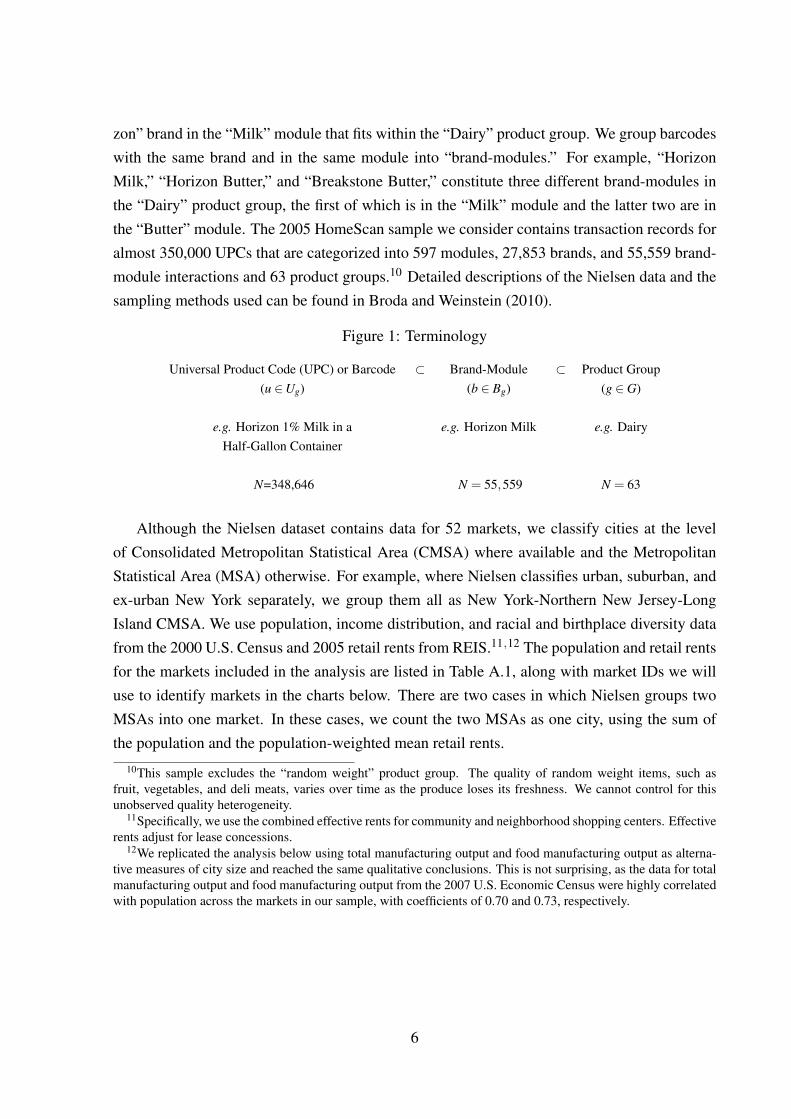
zon” brand in the “Milk” module that fits within the “Dairy” product group. We group barcodeswith the same brand and in the same module into “brand-modules.” For example, “HorizonMilk,” “Horizon Butter,” and “Breakstone Butter,” constitute three different brand-modules inthe “Dairy” product group, the first of which is in the “Milk” module and the latter two are inthe “Butter” module. The 2005 HomeScan sample we consider contains transaction records foralmost 350,000 UPCs that are categorized into 597 modules, 27,853 brands, and 55,559 brand-module interactions and 63 product groups.10 Detailed descriptions of the Nielsen data and thesampling methods used can be found in Broda and Weinstein (2010).

Figure 1: Terminology

Universal Product Code (UPC) or Barcode ⊂ Brand-Module ⊂ Product Group(u ∈Ug) (b ∈ Bg) (g ∈ G)

e.g. Horizon 1% Milk in a e.g. Horizon Milk e.g. DairyHalf-Gallon Container

N=348,646 N = 55,559 N = 63

Although the Nielsen dataset contains data for 52 markets, we classify cities at the levelof Consolidated Metropolitan Statistical Area (CMSA) where available and the MetropolitanStatistical Area (MSA) otherwise. For example, where Nielsen classifies urban, suburban, andex-urban New York separately, we group them all as New York-Northern New Jersey-LongIsland CMSA. We use population, income distribution, and racial and birthplace diversity datafrom the 2000 U.S. Census and 2005 retail rents from REIS.11,12 The population and retail rentsfor the markets included in the analysis are listed in Table A.1, along with market IDs we willuse to identify markets in the charts below. There are two cases in which Nielsen groups twoMSAs into one market. In these cases, we count the two MSAs as one city, using the sum ofthe population and the population-weighted mean retail rents.

10This sample excludes the “random weight” product group. The quality of random weight items, such asfruit, vegetables, and deli meats, varies over time as the produce loses its freshness. We cannot control for thisunobserved quality heterogeneity.

11Specifically, we use the combined effective rents for community and neighborhood shopping centers. Effectiverents adjust for lease concessions.

12We replicated the analysis below using total manufacturing output and food manufacturing output as alterna-tive measures of city size and reached the same qualitative conclusions. This is not surprising, as the data for totalmanufacturing output and food manufacturing output from the 2007 U.S. Economic Census were highly correlatedwith population across the markets in our sample, with coefficients of 0.70 and 0.73, respectively.

6

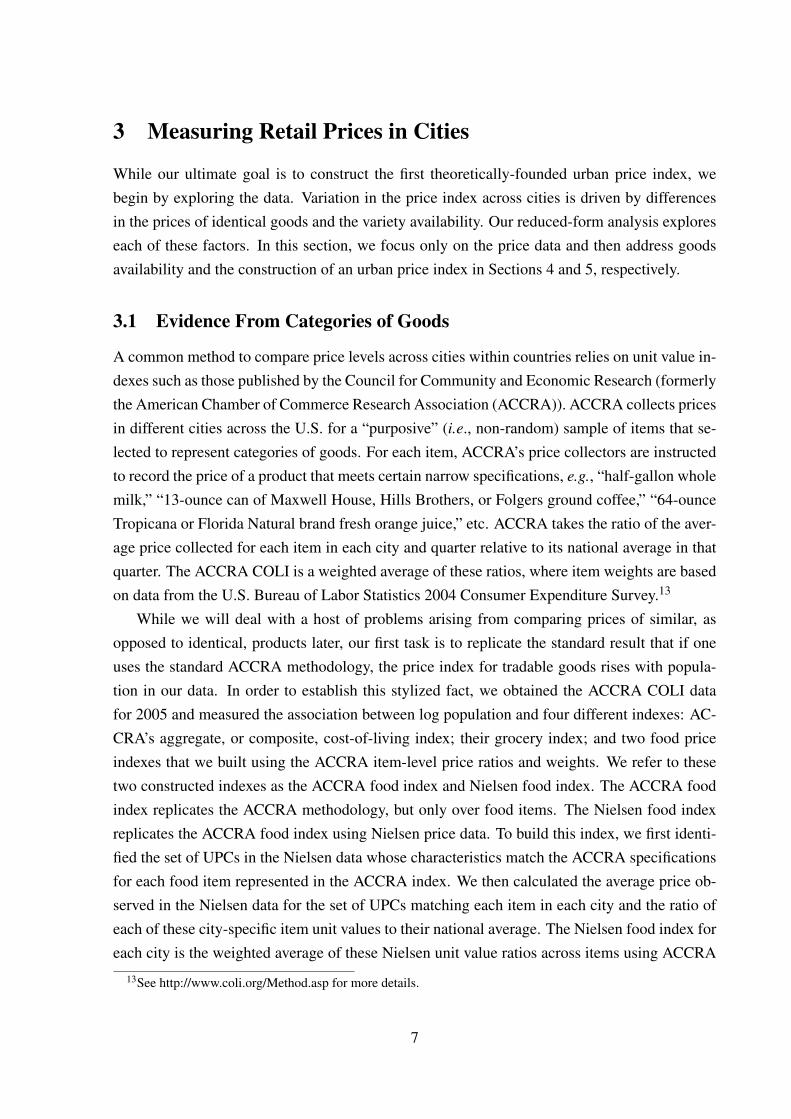
3 Measuring Retail Prices in Cities

While our ultimate goal is to construct the first theoretically-founded urban price index, webegin by exploring the data. Variation in the price index across cities is driven by differencesin the prices of identical goods and the variety availability. Our reduced-form analysis exploreseach of these factors. In this section, we focus only on the price data and then address goodsavailability and the construction of an urban price index in Sections 4 and 5, respectively.

3.1 Evidence From Categories of Goods

A common method to compare price levels across cities within countries relies on unit value in-dexes such as those published by the Council for Community and Economic Research (formerlythe American Chamber of Commerce Research Association (ACCRA)). ACCRA collects pricesin different cities across the U.S. for a “purposive” (i.e., non-random) sample of items that se-lected to represent categories of goods. For each item, ACCRA’s price collectors are instructedto record the price of a product that meets certain narrow specifications, e.g., “half-gallon wholemilk,” “13-ounce can of Maxwell House, Hills Brothers, or Folgers ground coffee,” “64-ounceTropicana or Florida Natural brand fresh orange juice,” etc. ACCRA takes the ratio of the aver-age price collected for each item in each city and quarter relative to its national average in thatquarter. The ACCRA COLI is a weighted average of these ratios, where item weights are basedon data from the U.S. Bureau of Labor Statistics 2004 Consumer Expenditure Survey.13

While we will deal with a host of problems arising from comparing prices of similar, asopposed to identical, products later, our first task is to replicate the standard result that if oneuses the standard ACCRA methodology, the price index for tradable goods rises with popula-tion in our data. In order to establish this stylized fact, we obtained the ACCRA COLI datafor 2005 and measured the association between log population and four different indexes: AC-CRA’s aggregate, or composite, cost-of-living index; their grocery index; and two food priceindexes that we built using the ACCRA item-level price ratios and weights. We refer to thesetwo constructed indexes as the ACCRA food index and Nielsen food index. The ACCRA foodindex replicates the ACCRA methodology, but only over food items. The Nielsen food indexreplicates the ACCRA food index using Nielsen price data. To build this index, we first identi-fied the set of UPCs in the Nielsen data whose characteristics match the ACCRA specificationsfor each food item represented in the ACCRA index. We then calculated the average price ob-served in the Nielsen data for the set of UPCs matching each item in each city and the ratio ofeach of these city-specific item unit values to their national average. The Nielsen food index foreach city is the weighted average of these Nielsen unit value ratios across items using ACCRA

13See http://www.coli.org/Method.asp for more details.

7

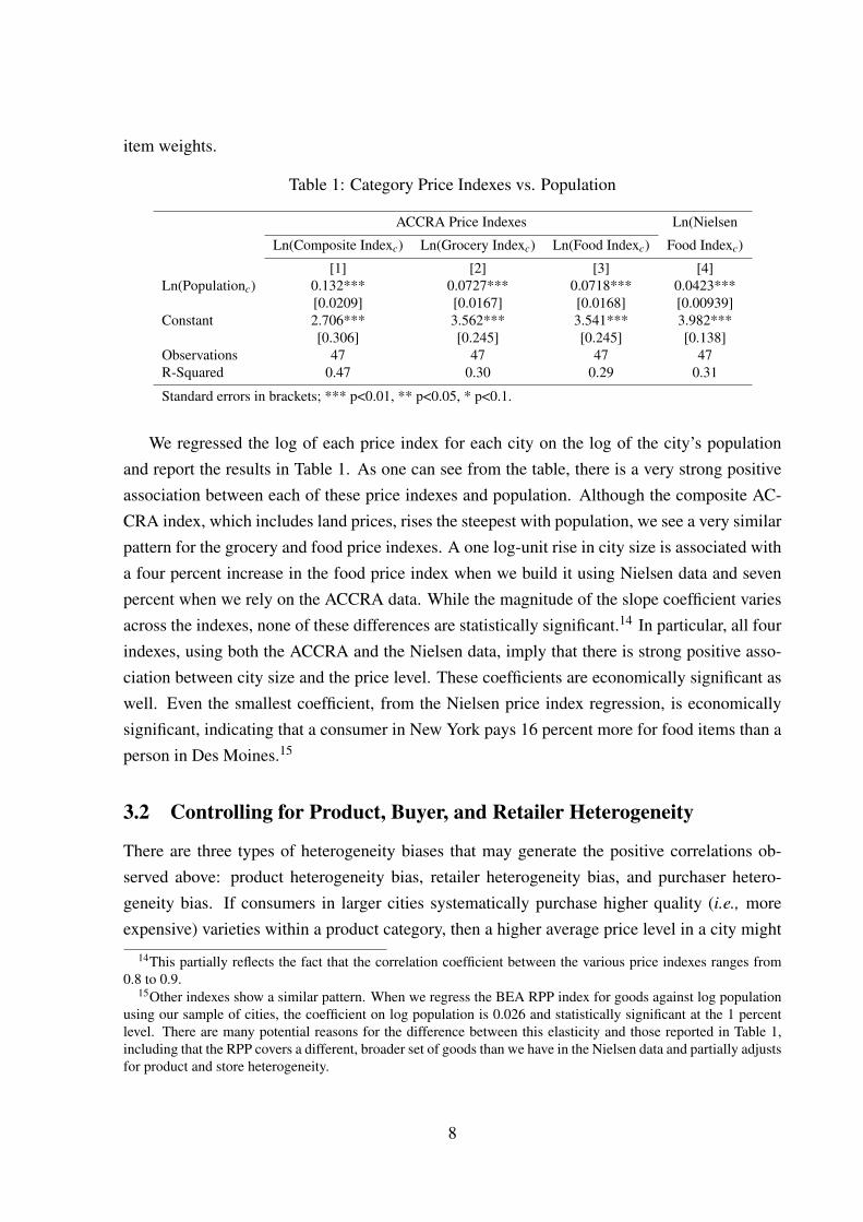
item weights.

Table 1: Category Price Indexes vs. Population

ACCRA Price Indexes Ln(Nielsen

Ln(Composite Indexc) Ln(Grocery Indexc) Ln(Food Indexc) Food Indexc)

[1] [2] [3] [4]Ln(Populationc) 0.132*** 0.0727*** 0.0718*** 0.0423***

[0.0209] [0.0167] [0.0168] [0.00939]Constant 2.706*** 3.562*** 3.541*** 3.982***

[0.306] [0.245] [0.245] [0.138]Observations 47 47 47 47R-Squared 0.47 0.30 0.29 0.31

Standard errors in brackets; *** p<0.01, ** p<0.05, * p<0.1.

We regressed the log of each price index for each city on the log of the city’s populationand report the results in Table 1. As one can see from the table, there is a very strong positiveassociation between each of these price indexes and population. Although the composite AC-CRA index, which includes land prices, rises the steepest with population, we see a very similarpattern for the grocery and food price indexes. A one log-unit rise in city size is associated witha four percent increase in the food price index when we build it using Nielsen data and sevenpercent when we rely on the ACCRA data. While the magnitude of the slope coefficient variesacross the indexes, none of these differences are statistically significant.14 In particular, all fourindexes, using both the ACCRA and the Nielsen data, imply that there is strong positive asso-ciation between city size and the price level. These coefficients are economically significant aswell. Even the smallest coefficient, from the Nielsen price index regression, is economicallysignificant, indicating that a consumer in New York pays 16 percent more for food items than aperson in Des Moines.15

3.2 Controlling for Product, Buyer, and Retailer Heterogeneity

There are three types of heterogeneity biases that may generate the positive correlations ob-served above: product heterogeneity bias, retailer heterogeneity bias, and purchaser hetero-geneity bias. If consumers in larger cities systematically purchase higher quality (i.e., moreexpensive) varieties within a product category, then a higher average price level in a city might

14This partially reflects the fact that the correlation coefficient between the various price indexes ranges from0.8 to 0.9.

15Other indexes show a similar pattern. When we regress the BEA RPP index for goods against log populationusing our sample of cities, the coefficient on log population is 0.026 and statistically significant at the 1 percentlevel. There are many potential reasons for the difference between this elasticity and those reported in Table 1,including that the RPP covers a different, broader set of goods than we have in the Nielsen data and partially adjustsfor product and store heterogeneity.

8

just reflect the fact that consumers in that city buy more expensive varieties of that product cat-egory. Similarly, retailer heterogeneity bias can arise because consumer in large cities mightpurchase goods in stores that offer systematically higher amenities. For example, some grocerystores, like Whole Foods, offer nicer shopping experiences than mass-merchandisers. Finally,if there are a higher fraction of wealthy people in large cities, and rich people look for bargainsless than poor people, purchaser heterogeneity might mean that purchase prices may reflectdifferent shopping intensities of consumers.

As we mentioned earlier, our objective is obtain a standardized price measure that reflectsthe prices of identical goods purchased in different locations but at similar stores and by con-sumers with similar shopping intensities. Essentially, we are trying to do the spatial equivalentto the time-series methodology employed in the construction of the U.S. Consumer Price In-dex, which measures price changes for identical products, purchased in the same store, by fieldagents with common shopping instructions.

Our methodology for doing this is quite straightforward. Let Pucrh be the average price thata household h paid for UPC u in store r in city c.16 We refer Pucrh as the “unadjusted price”and define pucrh as ln(Pucrh). We can then construct an adjusted price index by running thefollowing regression:

pucrh = αu +αc +αr +Zhβ + εucrh (1)

where αu, αc, and αr are UPC, city, and store fixed effects, respectively, and Zh denotes a vectorof household characteristics and β are the corresponding coefficients. Household demographicdummies are included for household size, as well as the gender, age, marital status, and race ofthe head of household; in addition, we control for household income, which is correlated withshopping intensity. Our store fixed effects take a different value for each of the approximately600 retail chains in our sample that serve at least 2 cities. For stores that we observe serving asingle city, we restrict αr to be the same for all stores of the same type, where type is defined inone of seven “channel-IDs”: grocery, drug, mass merchandiser, super-center, club, convenience,and other.17 The αr are designed to capture store amenities, and the Zhβ capture factors relatedto purchaser heterogeneity.

The city fixed effects, αc, can be thought of as city price indexes that control for the typesof products purchased, the store in which the purchase occurred, and the shopping intensity

16HomeScan panelists record purchases for each transaction they make while participating the survey and datarecords are identified using a calendar date. We aggregate the data to the annual frequency, summing purchasevalues and quantities across transactions in the 2005 sample. The average price paid is, therefore, the sum ofthe dollar amounts that a household h paid for UPC u in store r over all of the transactions where we observethe household purchasing that UPC in that store, divided by the sum of the number of units that the householdpurchased across the same set of transactions. We identify the “store” r that a transaction occurs in using Nielsen’sstore code variable.

17We apply the same restriction to stores whose codes refer to store categories (such as “Fish Market,” “CheeseStore,” etc.) rather than store names.

9

of the buyer. We then can test whether standardized urban prices co-vary with population byregressing the city fixed effects on log population, i.e.,

αc = α + γ ln(Popc)+ εc, (2)

where ln(Popc) is the log of population in city c. In this specification, γ tells us how prices varywith population after we control for the different bundles of products purchased in differentcities. An advantage of this two-stage approach as opposed to simply including co-variates ofinterest in equation (1) is that our city price level estimates are not affected by what we thinkco-varies with urban prices. Thus, we separate the question of whether urban prices rise withpopulation from the question of how to correctly measure urban prices. We will use this featureof the methodology in Section 5. However, as a robustness check, we will also show in Section3.4.1 that our two-stage approach is not qualitatively important for our results.

3.3 Evidence from Barcode Prices

Recall that in Section 3.1 above, we showed that products from the same category were pur-chased for higher unit values in larger cities. The results in Table 1 indicated that a one log unitrise in city size is associated with a four percent rise in the unit value of groceries. We will nowdemonstrate that almost all of this effect can be explained by product, retailer, and purchaserheterogeneity biases. In other words, past studies have found that there are higher traded goodsprices in larger cities because big cities have different (less price sensitive) consumers purchas-ing different (more expensive) varieties of products in different (more expensive) stores.

Table 2 presents results from estimating equations (1) and (2). The first key difference fromTable 1 is that we are now gauging price differences between identical products, or UPCs, soldin different cities.18 In the first column of the table, we present the results from a specificationthat only adjusts for product heterogeneity. In other words, instead of running the regressionspecified in equation (1), we compute the city price index by only regressing prices on UPCdummies and city dummies. This method for computing the price index corrects for productheterogeneity, which are contained in the UPC fixed effects, but does not adjust for purchaserand retailer heterogeneity. In the second panel, we report the results from regressing the es-timated city dummy coefficients on log population. We obtain a coefficient of 0.0139, whichis only one third as large as the coefficient we obtained in Table 1 when we used the ACCRAmethodology to generate a price index and regressed that on population. This result indicatesthat two-thirds of the positive relationship between prices and city size in the unit value indexreflects the fact that people in larger cities purchase far more high-priced varieties of goods than

18In all regressions, we weight the data by the transaction value which gives more weight to goods that constitutehigher expenditure shares.

10

residents of small cities.19

Table 2: Identical Product Price Indexes vs. Population

Panel A

p1ucrh

[1] [2] [3] [4]Ln(Incomeh) - 0.0114*** - 0.00805***

- [0.000961] - [0.000525]

UPC Fixed Effects Yes Yes Yes YesCity Fixed Effects Yes Yes Yes YesHousehold Demographic Dummies2 No Yes No YesStore Dummies3 No No Yes Yes

Observations 15,570,529 15,570,529 15,570,529 15,570,529Number of UPCs4 348,645 348,645 348,645 348,645R-Squared 0.948 0.948 0.953 0.953

Panel B

City Fixed Effect Coefficient from Panel A

[1] [2] [3] [4]Ln(Populationc) 0.0139*** 0.0130*** 0.00603*** 0.00568**

[0.00400] [0.00396] [0.00215] [0.00214]Constant -0.245*** -0.229*** -0.117*** -0.110***

[0.0586] [0.0581] [0.0315] [0.0314]

Observations 49 49 49 49R-Squared 0.916 0.205 0.187 0.143

Standard errors in brackets; *** p<0.01, ** p<0.05, * p<0.1. Panel A standard errors are clustered by city.

Notes:1. pucrh = ln(Pucrh) where Pucrh is the total expenditures by household h on UPC u in store r in city c in 2005 divided bythe total quantity of UPC u purchased by household h in store r in city c during 2005. Observations in thePanel A regression are weighted by the total expenditure of household h on UPC u in store r.2. Household demographic dummies are for household size, male and female head of household age, marital status,race, and hispanic.3. Regressions with store dummies include one of seven channel-ID dummies is Nielsen does not provide a store nameor the store identified only has sales in one city and a store name dummy otherwise.4. Random weight UPCs have been dropped from the sample.

In Column 2 of Table 2, we adjust the urban price index for both product heterogeneityand purchaser heterogeneity. The positive coefficient on household income indicates that highincome households systematically pay more for the same goods as poorer households. Some ofthis may be due to the fact that high-income households have a higher opportunity cost of timeand therefore shop less intensively and also have a greater willingness to shop in high amenitystores. Alternatively, some of this positive association may be due to the fact that stores that

19One possible concern with these results is that shifts in the weighting of the data or some other factor associatedwith the shift from the price index methodology to the regression methodology is responsible for the drop. Weinvestigate this possibility as a robustness check and show in Appendix Section C that this concern is not warranted.

11

cater to richer clientele are able to charge higher markups. While we will disentangle thesetwo forces later, for the time being we simply note that controlling for purchaser heterogeneitycauses the coefficient on log population to fall by another ten percent.

Interestingly, controlling for store fixed effects in Column 3 has a much more substantialimpact on the elasticity of urban prices with respect to population than controlling for purchaserheterogeneity: more than halving the coefficient. The large impact of controlling for storeheterogeneity implies that a second important reason why prices appear higher in larger citiesis that residents of large cities disproportionately shop in stores that charge high prices in all

cities. The most obvious source of this sort of heterogeneity is differences in amenities—richhouseholds tend to purchase nicer varieties of goods and shop in nicer stores—but we will alsoexamine the possibility that markup variations are explaining this in Section 3.4.2. Finally, ifwe control for both product, purchaser, and retailer heterogeneity in Column 4 the coefficientcollapses to only 13 percent of its magnitude in Table 1. Most of this fall arises from adjustingfor retailer heterogeneity, which reflects that shoppers in larger cities purchase more items inhigh-amenity stores. The coefficient on household income remains positive and significant,which means that richer households pay more for the same UPC even in the same store. Weinterpret this as evidence for the impact of purchaser heterogeneity on prices. Interestingly, themagnitude of the coefficient on income in Column 4 is about 70 percent as large as in Column2, indicating that most of the reason why richer households pay more for the same UPC is dueto their lower shopping intensity within stores and not to their choosing to shop in nicer stores.

Figure 2: Estimated Price Levels vs. Log City Population

DMLR

Oma

SyrAlb

Bir

Ric

Lou

GR

Jac

Mem

R−DNas

SLC

ChaCol

SA

Ind

OrlMil

NH

KC

NO

OkCCin

Por

B−RPitTam

DenStL

SDCle

Pho

Sea

Mia

Atl

Hou

Dal

Det

Bos

Phi

SF

DC

Chi

LA NY

−.2

0.2

.4Pr

ice

Inde

x

13 14 15 16 17ln(City Population)

Adjusted Nielsen Price Index Nielsen Food Price Index

Notes:1. The market labels on the ACCRA price indexes reference the city represented, as listed in Table A.1.2. City price indexes are normalized to be mean zero.

12

Figure 2 presents plots of price indexes computed using the ACCRA methodology in pre-sented in the final column of Table 1 and the price indexes generated in Column 4 of Table 2.The hollow circles indicate the price indexes computed using the ACCRA methodology and thesolid circles indicate those computed after correcting for the various forms of heterogeneity inthe data. As one can see from the plot, there is a dramatic collapse in the relationship betweenurban prices and population once one controls for product, purchaser, and retailer heterogene-ity. Indeed, the slight positive association that we identified in Table 2 is almost imperceptible,indicating that its economic significance is minor. Moreover, most of the dispersion in city priceindexes disappears once we control for heterogeneity yielding very small deviations from thefitted line. After adjusting for the various forms of heterogeneity bias, the variance in urbanprice levels falls by 95 percent. In other words, purchasing price parity for tradables hardlyvaries across US cities.

3.4 Robustness

In this section we consider two robustness checks. First, we demonstrate that our results aresimilar when we estimate the association between city population and prices in a one-step esti-mation procedure. Second, we demonstrate that our results are not due to variable markups.

3.4.1 One-Step Estimation Procedure

Thus far we have been working with a two-step procedure for estimating the association be-tween city population and prices. In Table 3 we repeat our exercise using a one-step procedurein which we replace the city fixed effects in equation (1) with the log of population in each city.The results are extremely similar to our earlier ones. The coefficients on log population are, inparticular, very close to their counterparts in Panel B of Table 2, which tells us that our choiceof a two-step procedure does not qualitatively affect the results.

3.4.2 Amenities vs. Mark-ups

One of the important adjustments that we make is for store amenities. Our methodology as-sumes that if consumers in a given city pay more for identical products when they buy themat one type of store relative to other stores within the same city, the higher price must reflecta difference in store amenities. An alternative explanation is that the higher price reflects ahigher markup. If stores that are prevalent in larger cities charge higher markups, our resultsmight be due to the fact that our method of eliminating retailer heterogeneity would be eliminat-ing markup variation across cities and therefore might be understating the high prices in largecities. In other words, if the store effects capture amenities, consumers do not necessarily find

13

Table 3: Are prices higher in larger cities?

p1ucrh

[1] [2] [3] [4]Ln(Populationc) 0.0155*** 0.0150*** 0.00650*** 0.00604***

[0.00267] [0.00363] [0.00223] [0.00219]Ln(Incomeh) - 0.00704*** - 0.00554***

- [0.00149] - [0.000727]

UPC Fixed Effects Yes Yes Yes YesHousehold Demographic Dummies2 No Yes No YesStore Dummies3 No No Yes Yes

Observations 15,570,529 15,570,529 15,570,529 15,570,529Number of UPCs4 348,645 348,645 348,645 348,645Number of Cities 49 49 49 49R-squared 0.947 0.947 0.953 0.953

Robust standard errors in brackets; *** p<0.01, ** p<0.05, * p<0.1. Standard errors are clustered by cityand storename/type in specifications where store dummies are included and city otherwise.

Notes:1. pucrh = ln(Pucrh) where Pucrh is the total expenditures by household h on UPC u in store r in city c in 2005 divided bythe total quantity of UPC u purchased by household h in store r in city c during 2005. Observations are weightedby the total expenditure of household h on UPC u in store r.2. Household demographic dummies are for household size, male and female head of household age, marital status,race, and hispanic.3. Regressions with store dummies include one of seven channel-ID dummies is Nielsen does not provide a store nameor the store identified only has sales in one city and a store name dummy otherwise.4. Random weight UPCs have been dropped from the sample.

big cities to be more expensive because they are getting a higher-quality shopping experiencein return for paying a higher price. If the store effects instead reflect markup differences dueto differences in market power across stores offering the same shopping experience, then con-sumers are not getting anything in return for the relatively high prices charged by stores in largecities and will, therefore, perceive these stores as more expensive.

Although we cannot measure markups directly, we can look at store market share informa-tion in an attempt to assess how markups might vary in our data, first across cities, and thenacross retailers and, in particular, across retailers that locate disproportionately in large, rela-tive to small, cities. In many variable markup demand systems involving strategic substitutes,markups positively covary with market shares. For example, Feenstra and Weinstein (2010)show that for the translog system, markups will positively covary with the Herfindahl indexin the market. We can compute retailer Herfindahl indexes for each city by aggregating thepurchases of consumers in each store. Not surprisingly, Herfindahl indexes are negatively cor-related with city size (ρ =−0.3) reflecting the fact that consumers in large cities not only havemore choices of products, but also more choices of where to purchase those products. This cir-cumstantial evidence suggests that, if anything, we are understating the amenity effect because

14

stores in large cities are likely to face more competition and charge lower markups (which isalso consistent with models like Melitz and Ottaviano (2008)).

We also can try to strip out the market power effect from our estimates more directly. Inorder to do this we control for differences in markups across retail chains, or types, by includingstore market shares in the regression where we estimate the store effects (αr).20 Specifically,we add the market share of each store in each city to equation (1) and estimate

pucrh = αu +αc +αr +Zhβ + γSharerc + εucrh, (3)

where Sharerc is store r’s market share in city c and γ is a parameter to be estimated. Weinterpret αr in this specification as the component of the store’s idiosyncratic price that cannotbe explained by its market power. We then subtract these αr estimates from observed prices,adjusting prices for the component that is potentially related to differences in amenities, but notthe component related to differences in markups via market power. We regress these adjustedprices against city fixed effects to estimate urban price indexes that control for differences inamenities across stores, but still allow for price differences resulting from differences in marketpower:

pucrh− αr = αu + αc +Zhβ + εucrh, (4)

The dependent variable is the store amenity-adjusted price and αc is an urban price index thatreflects systematic differences in prices across stores with different market shares, but not thoserelated to unobserved heterogeneity between stores.

Table 4 presents the results of this exercise. The estimates for equation (3), in Column 1,suggest no significant relationship between a store’s market share in a market and the price itcharges.21 The coefficient on market share is positive but not statistically significant, indicatingthat the capacity of a retailer to exercise market power is quite limited in most cities.22

Column 2 presents the results of estimating the price indexes according to equation (4), andColumn 3 presents the results of regressing the resulting adjusted city fixed effects, αc, againstpopulation. Not surprisingly, given the lack of a significant effect in Column 1, we do not findthat adjusting for market share qualitatively affects our results. The city price indexes that have

20Recall that r denotes the store code for each transaction. Most store codes uniquely identify retail chains orstandalone stores; others refer to one of 60 store categories. If a store only has sales in one city or we do not havethe store name, we restrict αr to be equal across stores with the same “channel-ID,” which can take one of sevenvalues: grocery, drug, mass merchandiser, super-center, club, convenience, and other. We do not group stores inthis manner when calculating market shares: Sharerc represents the sales share of store code r in city c.

21We also tried non-linear specifications linking store shares with market power by including quadratic andcubic terms without finding a significant link.

22This result is consistent with the previous literature on retailer market power in the U.S. grocery sector whichfinds that stores do not exploit market power in their pricing decisions. For example, Ellickson and Misra (2008)demonstrate that “stores in a particular market do not use pricing strategy as a differentiation device but insteadcoordinate their actions” and find that “firm size is not the primary determinant of pricing strategy.”

15

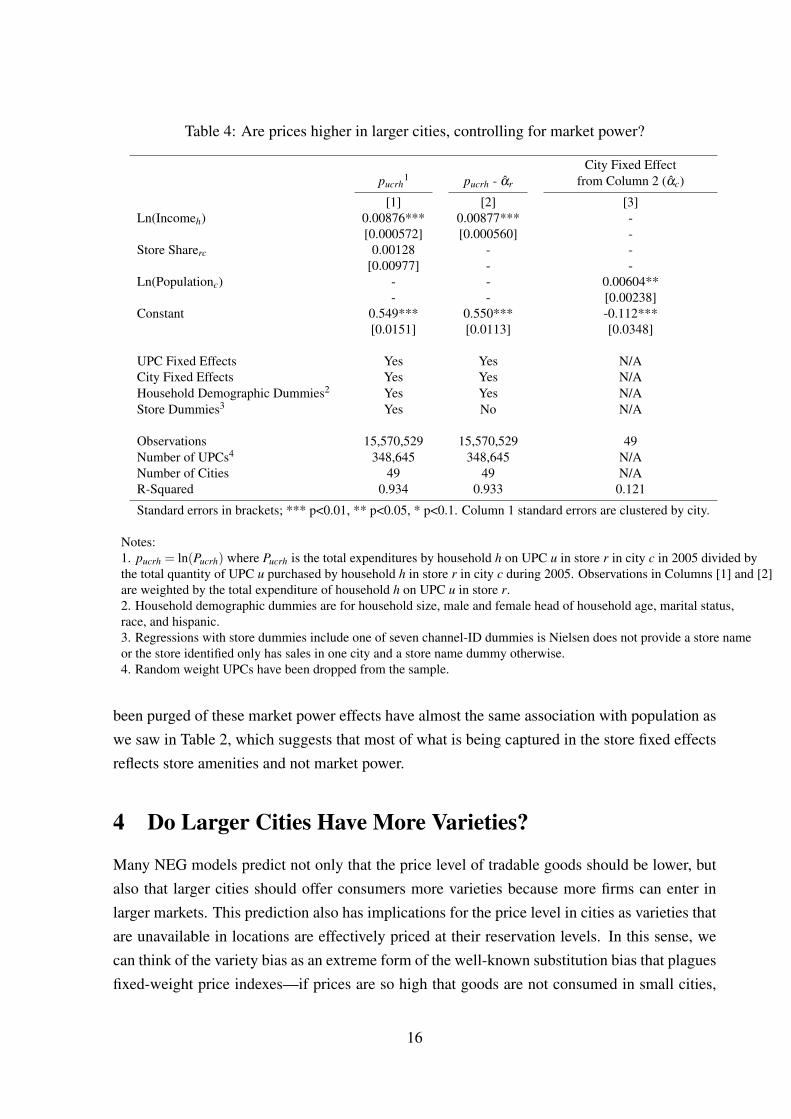
Table 4: Are prices higher in larger cities, controlling for market power?

City Fixed Effectpucrh

1 pucrh - αr from Column 2 (αc)

[1] [2] [3]Ln(Incomeh) 0.00876*** 0.00877*** -

[0.000572] [0.000560] -Store Sharerc 0.00128 - -

[0.00977] - -Ln(Populationc) - - 0.00604**

- - [0.00238]Constant 0.549*** 0.550*** -0.112***

[0.0151] [0.0113] [0.0348]

UPC Fixed Effects Yes Yes N/ACity Fixed Effects Yes Yes N/AHousehold Demographic Dummies2 Yes Yes N/AStore Dummies3 Yes No N/A

Observations 15,570,529 15,570,529 49Number of UPCs4 348,645 348,645 N/ANumber of Cities 49 49 N/AR-Squared 0.934 0.933 0.121

Standard errors in brackets; *** p<0.01, ** p<0.05, * p<0.1. Column 1 standard errors are clustered by city.

Notes:1. pucrh = ln(Pucrh) where Pucrh is the total expenditures by household h on UPC u in store r in city c in 2005 divided bythe total quantity of UPC u purchased by household h in store r in city c during 2005. Observations in Columns [1] and [2]are weighted by the total expenditure of household h on UPC u in store r.2. Household demographic dummies are for household size, male and female head of household age, marital status,race, and hispanic.3. Regressions with store dummies include one of seven channel-ID dummies is Nielsen does not provide a store nameor the store identified only has sales in one city and a store name dummy otherwise.4. Random weight UPCs have been dropped from the sample.

been purged of these market power effects have almost the same association with population aswe saw in Table 2, which suggests that most of what is being captured in the store fixed effectsreflects store amenities and not market power.

4 Do Larger Cities Have More Varieties?

Many NEG models predict not only that the price level of tradable goods should be lower, butalso that larger cities should offer consumers more varieties because more firms can enter inlarger markets. This prediction also has implications for the price level in cities as varieties thatare unavailable in locations are effectively priced at their reservation levels. In this sense, wecan think of the variety bias as an extreme form of the well-known substitution bias that plaguesfixed-weight price indexes—if prices are so high that goods are not consumed in small cities,

16

fixed-weight indexes will understate the true cost of living because high-priced goods that arenot consumed will receive a weight of zero in the index. While we will deal with both thesubstitution and variety biases in Section 5, in this section we examine the underlying evidenceon variety availability.

4.1 Data Overview

The simplest way to document that consumers in larger cities consume more varieties is toexamine whether we observe more varieties being purchased in larger cities. Figure 3 showsthe relationship between the log number of UPCs observed in the Nielsen sample for eachcity against log population. This relationship is upward sloping with a coefficient of 0.312and standard error of 0.043. We cannot interpret this estimate as the elasticity of variety withrespect to city size, however, because it is affected by sample bias: Nielsen tends to samplemore households in larger cities.

Figure 3: Log Number of Distinct UPCs in Each City Sample vs. Log City Population

DM

LR

Oma

Syr Alb

Bir

Ric

Lou

GR

Jac

Mem

R−D

Nas

SLC

ChaCol

SA

IndOrl

Mil

NHKC

Sac

NOOkC

Cin

Por

B−R

Pit

TamDenStL

SD

Cle

MinPhoSeaMia

AtlHouDal

DetBos

Phi

SF

DC

Chi LA

NY

1010

.511

11.5

Ln(N

umbe

r of U

PCs)

13 14 15 16 17Ln(Population)

Ln(No. of Distinct UPCs Purchased by Sample HHs) Fitted values

Notes:1. Numbers on plots reference the market ID of the city represented, as listed in Table A.1.

One way to deal with this bias is to instead examine whether the number of different vari-eties consumed by an equal number of households varies with city size. The basic idea is thatany two households are less likely to purchase the same product in markets where there aremore products to choose from. If there is less overlap in the varieties purchased by differenthouseholds in larger cities, we expect to see equally-sized samples of households from thesecities purchasing larger numbers of unique varieties.

We therefore restrict ourselves to only looking at 25 cities in which Nielsen sampled atleast 500 households and compare the number of varieties purchased by a random sample of

17

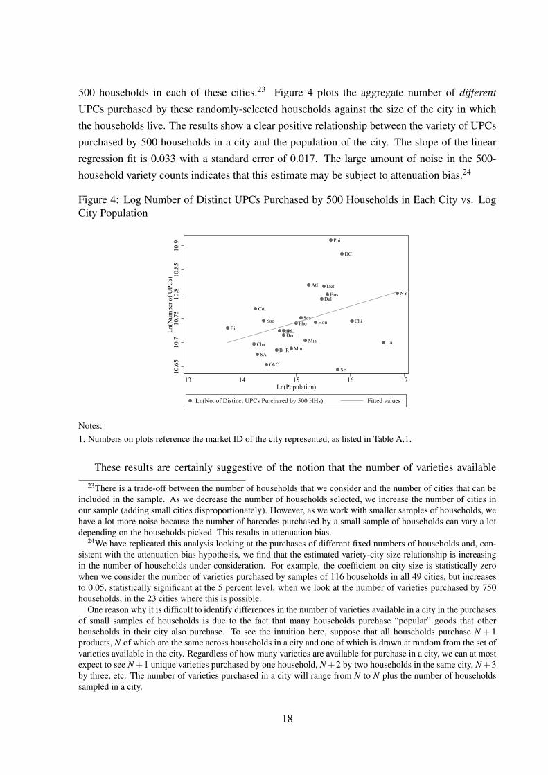
500 households in each of these cities.23 Figure 4 plots the aggregate number of different

UPCs purchased by these randomly-selected households against the size of the city in whichthe households live. The results show a clear positive relationship between the variety of UPCspurchased by 500 households in a city and the population of the city. The slope of the linearregression fit is 0.033 with a standard error of 0.017. The large amount of noise in the 500-household variety counts indicates that this estimate may be subject to attenuation bias.24

Figure 4: Log Number of Distinct UPCs Purchased by 500 Households in Each City vs. LogCity Population

Bir

Cha

Col

SA

Sac

OkC

B−R

TamDenStL

Min

PhoSea

Mia

Atl

Hou

Dal

DetBos

Phi

SF

DC

Chi

LA

NY

10.6

510

.710

.75

10.8

10.8

510

.9Ln

(Num

ber o

f UPC

s)

13 14 15 16 17Ln(Population)

Ln(No. of Distinct UPCs Purchased by 500 HHs) Fitted values

Notes:1. Numbers on plots reference the market ID of the city represented, as listed in Table A.1.

These results are certainly suggestive of the notion that the number of varieties available

23There is a trade-off between the number of households that we consider and the number of cities that can beincluded in the sample. As we decrease the number of households selected, we increase the number of cities inour sample (adding small cities disproportionately). However, as we work with smaller samples of households, wehave a lot more noise because the number of barcodes purchased by a small sample of households can vary a lotdepending on the households picked. This results in attenuation bias.

24We have replicated this analysis looking at the purchases of different fixed numbers of households and, con-sistent with the attenuation bias hypothesis, we find that the estimated variety-city size relationship is increasingin the number of households under consideration. For example, the coefficient on city size is statistically zerowhen we consider the number of varieties purchased by samples of 116 households in all 49 cities, but increasesto 0.05, statistically significant at the 5 percent level, when we look at the number of varieties purchased by 750households, in the 23 cities where this is possible.

One reason why it is difficult to identify differences in the number of varieties available in a city in the purchasesof small samples of households is due to the fact that many households purchase “popular” goods that otherhouseholds in their city also purchase. To see the intuition here, suppose that all households purchase N + 1products, N of which are the same across households in a city and one of which is drawn at random from the set ofvarieties available in the city. Regardless of how many varieties are available for purchase in a city, we can at mostexpect to see N +1 unique varieties purchased by one household, N +2 by two households in the same city, N +3by three, etc. The number of varieties purchased in a city will range from N to N plus the number of householdssampled in a city.

18

in a location rises with number of inhabitants in that location, but neither provides a reliableestimate of the elasticity. In the next section, we take a more direct approach to estimating thevariety-city size relationship: we use all of the information at hand to estimate the total numberof varieties available in each location and then examine how these aggregate variety estimatesvary with city size.

4.2 Estimating the Number of Varieties in Cities

The principle challenge that we face in measuring the number of varieties in a city is that ourdata is not a census of all varieties purchased in a city but rather a count of varieties basedon a random sample of households. Fortunately, our problem is isomorphic to a well-studiedproblem in biostatistics: estimating the number different species in a general area based onthe number of species identified in certain locations (see Mao et al. (2005, 2004)). Prior workin this area has solved the problem using parametric and structural approaches that yield verysimilar results in our data. Since the parametric approach is significantly simpler to explain, wefocus on the parametric approach and relegate the the structural approach to Appendix A as arobustness check.

In order to obtain some intuition for this methodology, assume that the expected numberof different products purchased by one household in city c is denoted by Sc (1). The expectednumber of distinct products purchased in a sample of n households can be denoted by the “accu-mulation curve,” Sc (n). Accumulation curves must be concave because every time the samplesize rises by one household the probability of finding good that has not been purchased by anyof the other households falls. Moreover, a critical feature of accumulation curves is that as thenumber of households surveyed rises, the number of observed varieties in a city must approachthe true total number of varieties in a city. We can write this formally as limn→∞ Sc (n) = ST

c ,where ST

c is the total number of distinct varieties available in the city.25 In other words, theasymptote of the accumulation curve is the estimate for the total number of goods available inthe city.

Estimation of STc requires us to know the expected value of distinct varieties for each sample

of households, i.e., (Sc(1),Sc(2),Sc(3), . . . ), and also the functional form of Sc (n). Estimat-ing the expected number of distinct varieties purchased by a sample of n households, Sc (n) isstraightforward. The only econometric issue we face is that the number of distinct varietieswe observe being purchased, Sc (n), in a sample of n households is going to depend on exactlywhich households are in the sample. For example, our measure of Sc(1), how many differentgoods one household purchases, depends on which household is chosen. In order to obtain an

25This property is based on the assumption that all types of varieties have a positive probability of being pur-chased.

19

estimate of the expected number of goods purchased by a sample of n households, Colwell andCoddington (1994) propose randomizing the sample order I times and generating an accumula-tion curve for each random ordering indexed by i. The expected value of the number of varietiespurchased by n households can then be set equal to the mean of the accumulation curves over I

different randomizations, i.e.,

Sc(n) =1I

I

∑i=1

Sci(n).

We set I = 50.26

Once we have our estimates for each Sc (n), we can turn to estimating the asymptote,Sc (Hc) = ST

c . Unfortunately, theory does not tell us what the functional for of Sc (n) is, sowe follow Jimenez-Valverde et al. (2006) by estimating the parameters of various plausiblefunctional forms and use the Akaike Information Criterion (AIC) goodness-of-fit test to choosebetween a range of functional forms that pass through the origin and have a positive asymptote.

4.3 Results

We can get a clear sense of how this methodology works by simply plotting the accumulationcurves. Figure 5 presents a plot of accumulation curves for the twelve cities for which we havethe largest samples. As one can see from the picture, the average sample of 1000 households inPhiladelphia (population 6.2 million) purchased close to 70,000 different varieties of groceries.By contrast, the average sample of a 1000 households in Saint Louis (population 2.6 million)purchased closer to 50,000 different varieties. Moreover, these curves reveal that the four high-est curves correspond to Philadelphia, D.C.-Baltimore, New York, and Boston, which are allamong the five largest cities in our sample. In other words, this limited sample indicates that agiven number of households tends to purchase a more diverse set of goods when that sample isdrawn from a city with a larger population.

We can examine this more formally by estimating the asymptotes of the accumulationcurves. Since we are not sure how to model the functional forms of these accumulation curves,we tried five different possible functional forms – Clench, Chapman-Richards, Morgan-Mercer-Flodin, Negative Exponential, and Weibull. We choose among these based on the Akaike In-formation Criterion (AIC). The Weibull was a strong favorite with the lowest AIC score in themajority of cities for which we modeled UPC count accumulation curves, and so we decided tofocus on this functional form.

Once again, we can get intuition for how this methodology works by showing the fit for asub-sample. Figure 6 plots the raw data and the estimated Weibull accumulation curve for our

26The resulting estimates are less noisy, and their correlation with city size less subject to attenuation bias, thanthe 500-household variety counts studied in Section 4.1 above, each of which is just a single point on a singleaccumulation curve for each city.

20

Figure 5: UPC Accumulation Curves for Markets with 12 Largest Samples

020

000

4000

060

000

8000

0N

umbe

r of U

PCs i

n sa

mpl

e

0 500 1000 1500Number of households in sample

PHILADELPHIA

D.C.−BALTIMORE

NEW YORK

BOSTON

COLUMBUS

SEATTLE

PHOENIX

TAMPA

DENVER

LOS ANGELES

MINNEAPOLIS

ST. LOUIS

Cities Listed inOrder of Curve Height

largest city, New York. A typical sample of 500 random households buys around 49,000 uniqueUPCs, and a sample of 1000 households typically purchases around 66,000 different goods. Asone can see from the plot, the estimated Weibull distribution fits the data extremely well. Theestimated asymptote is approximately 112,000 varieties, which is 35,000 more than we observein our sample of 1500 New York households.27

Figure 7 presents a plot of the log of the estimated Weibull asymptotes for each city againstthe log population in the city. As one can see, there is a clear positive relationship betweenthe two variables—we estimate that households in larger cities have access to more varietiesthan households in smaller ones. It is interesting that the relationship between city size andthe total number of varieties in a city is much stronger than the relationship between city sizeand the number of varieties purchased by a fixed sample of cities observed in Figure 4. Thisis consistent with the pattern observed in Figure 5: there is less dispersion in the number ofunique UPCs purchased by a common set of household across cities increases as the number ofhousehold in that set increases. Overall, the data support relationship between the size of a cityand the number of varieties available hypothesized by NEG models. Residents of New Yorkhave access just over 110,000 different varieties of groceries, while residents of small cities like

27Since the number of households in a city is large, we obtain almost identical results regardless of whether setthe number of varieties equal to Sc (Hc) or Sc (∞).

21

Figure 6: Fitted UPC Accumulation Curve for New York

050

000

1000

00N

umbe

r of U

PCs

0 2000 4000 6000 8000 10000Number of households

Accumulation Curve Fitted Weibull Weibull Asymptote

Weibull: y = 111838 * [1−exp(−.011 x^.641)]

Omaha and Des Moines have access to fewer than 24,000.

Figure 7: Log Weibull Variety Estimate vs. Log City Population

DM

LR

Oma

Syr Alb

Bir

Ric

Lou

GRJac

MemR−D

Nas

SLC

ChaCol

SA

IndOrl

MilNHKC

Sac

NOOkCCin

Por

B−R

Pit

Tam

DenStL

SD

Cle

MinPhoSeaMiaAtlHouDal

DetBos

Phi

SF

DC

Chi LA

NY

10.5

1111

.512

Ln(W

eibu

ll A

sym

ptot

e)

13 14 15 16 17Ln(Population)

Ln(Weibull Variety Estimate) Fitted values

Notes:1. Acronyms on plots reference the city represented, as listed in Table A.1.

We test this relationship between city size and variety abundance formally in Table 5. Table5 presents the results from regressing the log estimated number of varieties in a city on the log

22

of the population in the city. The first three columns of the table present regressions of thelog sample counts of varieties in each city on the log of the city’s population. The next threecolumns present regressions of the log estimate of number of varieties based on the Weibullasymptotes on city size. As one can see from comparing columns 1 and 4, the elasticity ofvariety with respect to population is slightly less using the Weibull estimate presumably becausethe Weibull corrects for the correlation between sample size and population in the Nielsen data.What is most striking, however, is that we observe a very strong and statistically significantrelationship between the size of the city and the number of estimated varieties. Our estimatesindicate that a city with twice the population as another one typically has 20 percent morevarieties.

Table 5: Do larger cities have more UPC varieties?

Ln(Sample Countc) Ln(Weibull Asymptotec)

[1] [2] [3] [4] [5] [6]Ln(Populationc) 0.312*** 0.338*** 0.281*** 0.289*** 0.317*** 0.321***

[0.0432] [0.0678] [0.0971] [0.0373] [0.0582] [0.0841]Ln(Per Capita Incomec) - -0.155 -0.043 - -0.032 -0.038

- [0.341] [0.369] - [0.293] [0.319]Income Herfindahl Index - -0.952 -0.289 - -1.302 -1.338

- [3.132] [3.246] - [2.689] [2.809]Race Herfindahl Index - 0.064 0.115 - 0.147 0.145

- [0.411] [0.417] - [0.353] [0.361]Birthplace Herfindahl Index - 0.006 0.029 - 0.068 0.067

- [0.282] [0.285] - [0.222] [0.225]Ln(Land Areac) - - 0.087 - - -0.005

- - [0.106] - - [0.0919]Constant 6.158*** 7.474** 6.275* 6.835*** 6.790** 6.856**

[0.632] [3.391] [3.704] [0.546] [2.911] [3.205]Observations 49 49 49 49 49 49R-squared 0.53 0.53 0.54 0.56 0.57 0.57

Standard errors in brackets; *** p<0.01, ** p<0.05, * p<0.1

One concern with these results is that they might be biased because larger cities have morediverse populations. In order to control for this we constructed a number of Herfindahl indexesbased on the shares of MSA population with different income, race, and country of birth. Theseindexes will be rising in population homogeneity. In addition, we include the per capita incomein each city. As one can see from columns 2 and 5 in Table 5, controlling for urban income anddiversity does not alter the results.

Finally, we were concerned that our results might be due to a spurious correlation betweencity population and urban land area. If there are a constant number of unique varieties per unitarea, then more populous cities might appear to have more diversity simply because they oc-cupy more area. To make sure that this force was not driving our results, we include the log ofurban land area in our regressions. The coefficient on land area is not significant in any of the

23

specifications, while the coefficient on population remains positive and very significant. Theseresults indicate that controlling for land area and demographic characteristics does not qualita-tively affect the strong relationship between city size and the number of available varieties. TheR2 of around 0.5 to 0.6 indicates that city size is an important determinant of variety availability.Thus, the number of tradable goods varies systematically with city size as hypothesized by theNEG literature.

5 The Price Level in Cities

5.1 Constructing an Exact Urban Price Index

In order to produce a theoretically-sound price index for a city, we need to take into account notonly the heterogeneity measurement issues discussed in section 3 and the product availabilitydifferences discussed in Section 4 but also make adjustments for substitution biases. Progresscan only be made by putting some more structure on the problem, and so we will assume thatone can use a CES utility function to measure welfare in cities. The CES has the advantage ofnot only being tractable and estimatable, but also has been used in many economic geographymodels, such as Krugman (1991), so our results can be thought of as a reasonable structuralestimate of what the price level is in this framework. Moreover, Feenstra and Weinstein (2010)show that this index yields very similar aggregate price levels to the translog (which is a second-order approximation of an arbitrary expenditure system) even when the number of varieties isvarying. Thus, the CES assumption is unlikely to dramatically affect our results relative to othercommonly used price indexes.28

Feenstra (1994) developed the variety-adjusted price index for the CES utility function.Here, we will modify it so that it can be used with our data. In the original Feenstra paper,the price index was expressed in terms of price level in period t as compared to t− 1. Insteadof working with two time periods, we modify the notation of the basic theory so that we cancompare two locations. In particular, we will express the price level in each city as its levelrelative to the price level a consumer would face if the buyer faced the average price level in theU.S. and had access to all the varieties available in the U.S. This approach enables us to writethe price level in every city relative to the the same U.S. national benchmark, which greatly

28Given that the median number of UPCs purchased in a module by a single person household (conditional onpurchasing anything in the module) is one, the data suggest that one should think of households as having hetero-geneous ideal-type preferences, as opposed to the identical CES preferences that form the theoretical foundationfor the variety-adjusted exact prices indexes used in this paper. This discrepancy, however, is not a problem forour analysis if we think of consumers as having a logit demand system. In particular, Anderson et al. (1987) havedemonstrated that a CES demand system can arise from the aggregation of ideal-type logit consumers. We willtherefore follow Anderson et al. (1987) and use the CES structure to evaluate aggregate welfare even though weknow that the discrete choice model is a better depiction of reality at the household level.

24

simplifies the analysis.

5.1.1 Intuition

It is worth spending a little time on the intuition behind this index before plunging into thedetail. Feenstra’s basic insight was that a variety-adjusted CES exact price index (EPI) can bewritten as a standard CES price index, which we term the “Conventional Exact Price Index”or CEPI, multiplied by a “Variety Adjustment” or VA term. The CEPI is a sales-weightedaverage of the prices of each good sold in the city where the weights adjust for conventionalsubstitution effects. In our context, one can think of the CEPI in city c, CEPIc, as the correctway of measuring the price level of the commonly available goods within each product groupin city c relative to their national average price.

Since some goods are not available in each location, we need to adjust the CEPIc by thevariety adjustment VAc. The variety adjustment corrects the price index for the impact of miss-ing varieties on consumer utility. It is based on two factors: the quality-weighted count of thegoods unavailable in a location and the substitutability of these missing goods with other goodsthat are available in a location. The quality-weighted count of missing goods weights each goodby how important it is in the utility function. Controlling for price, consumers will care moreabout not having access to high-quality varieties more than low-quality ones. In the CES setup,if two goods of have the same price, their relative market shares will be determined by theirrelative qualities. So, if consumers in a city do not have access to a good with a high national

sales share, we know that they are missing a good with greater importance (or price-adjustedquality) than they would be missing if they could not buy a good with a low market share. Asa result, the national market shares of goods not available in a location properly captures thequality-adjusted count of the unavailable goods.

The second adjustment comes from knowing the substitutability of the goods. Not havingaccess to a good without close substitutes is worse than not having access to a goods with closesubstitutes. In order to account for this force empirically, we follow Broda and Weinstein (2010)by allowing consumers to value not having access to an entire brand-module differently thannot having access to a good within a brand-module. For example, if Coke and Pepsi both selltwo soft-drink barcodes under each of their brands (cans and two-liter bottles), it may be worsefor consumers in a location not to have access to any Coke items than to not have access to justtwo-liter bottles. In terms of the formulas, this will require us to weight our quality-adjustedcounts of missing products in a location by how similar those products are to products that areavailable in that location.

25

5.1.2 Notation

Before actually writing down the price index, we need to set forth some notation to make theseconcepts concrete. Our first task is to compute the quality-weighted counts of missing goodsin each city that we can feed into our price index. Let g ∈ {1, ...,G} denote a product “group”,which we define in the same way as Nielsen to capture broadly similar grocery items. Let Bg

and Ug respectively denote the set of all “brand-modules” and UPCs in a product group g, andUb be the set of all UPCs in brand-module b.

Not all UPCs are sold in every city, so we now define the subsets of UPCs that we observebeing purchased. Let vuc denote the value of purchases of UPC u observed in the sample forcity c.29 We define Ubc ≡ {u ∈Ub|vuc > 0} as the set of all UPCs in brand-module b that havepositive observed sales in city c, and Ugc ≡ {u ∈Ug|vuc > 0} as the set of all UPCs in productgroup g that have positive observed sales in city c. We similarly define Bgc≡{b∈Bg|∑u∈b vuc 6=0} as the set of all brand-modules that have positive sales in city c in product group.

We next need to measure the share of available goods both within brand-modules and withinproduct groups. The simplest of these to construct is the share of available UPCs within a brand-module. Let sbc be share of national expenditures on brand-module b on UPCs Ubc that are soldin city c, i.e.,

sbc ≡∑u∈Ubc ∑c vuc

∑u∈Ub ∑c vuc. (5)

sbc tells us the expenditure share of UPCs within a brand-module that are available in a cityusing national weights. The numerator is the total amount spent nationally on all the goodsavailable in city c on UPCs in brand-module b, while the denominator gives the total spenton brand-module b nationally. This ratio will be less than one whenever a UPC from brand-module b is unavailable in city c. Another way to think about this variable is to realize that sbc

is positively related to the number of available UPCs in a city and will be smaller if, holdingfixed the number of unavailable UPCs, varieties with a high market share are unavailable. Itis easiest to see what moves sbc by considering an extreme case. If all varieties had the sameprice and quality and therefore the same market share, sbc would equal the share of all varietieswithin a brand-module that are available in city c, and sbA would equal sbB only if cities A andB had the same number of UPCs available in brand-module b. In general, however, two citieswith the same number of UPCs available in brand-module b will have equal values of sbc if theirunavailable varieties have the same aggregate importance in national consumption, or nationalexpenditure share.

29The national average price of a UPC is the total value of purchases of that UPC across all cities in the HomeS-can sample divided by the total quantity that these purchases represent. In all of the analysis below, we work withnationally-representative values and quantities for each UPC, scaling the value and quantity of purchases in eachcity by the population in that city divided by the total number of household members represented in the Nielsensample for that city (i.e., the sum of the household sizes for the Nieslen sample households).

26

We define a quality-weighted count of the brand-modules available in a location analo-gously:

sgc ≡∑

b∈Bgc

∑c

vbc

∑b∈Bg

∑c

vbc, where vbc = ∑

u∈Ub

vuc, (6)

and sgc is the expenditure share of brand-modules within product group g that are available incity c. The numerator of sgc is the total amount spent nationally on the product group g brand-modules available in city c, and its denominator is the total spent on product group g nationally.While sbc tells us about the availability of UPCs within brand-modules, sgc tells us about theavailability of brand-modules themselves.

Finally, it is useful to discuss the price data we use in the index. In our preferred speci-fication, we will work with “adjusted prices” that correct for product, purchaser, and retailerheterogeneity biases. In the simplest case, where we only control for product heterogeneitybiases, we set the adjusted price, Pucrh, equal to the the actual price: Pucrh ≡ Pucrh = exp{pucrh}.However, at other times we may want to correct for product and purchaser heterogeneity bi-ases in the collection of price data that we documented in Section 3. In this case, we willset Pucrh ≡ exp

{pucrh−Zhβ

}, or to correct for product, purchase, and retailer heterogeneity

biases we will set prices equal to Pucrh ≡ exp{

pucrh− αr−Zhβ

}. Similarly, we can write

the adjusted value and quantity of UPC u purchased in city c as vuc ≡ ∑h∈Hc

∑r∈Rc

Pucrhqucrh and

quc≡ ∑h∈Hc

∑r∈Rc

qucrh, respectively, where qucrh is the quantity that household h in city c purchases

of UPC u in store r.

5.1.3 Definition

We define a variety-adjusted spatial price index is based on Broda and Weinstein (2010)’s ex-tension of the Feenstra (1994) index. This extension is exact to a nested CES utility functionand was developed in order to measure inflation over barcoded products, nested according toNielsen categories defined above. We adapt Broda and Weinstein (2010)’s intertemporal priceindex to a spatial context, re-writing their Proposition 1 as follows:

Proposition 1. If Bgc 6= /0 for all g ∈ G, then the exact price index for the price of the set of

goods G in city c relative to the nation as a whole that takes into account the differences in

variety in the two locations is given by,

EPIc = ∏g∈G

[CEPIgcVAgc]wgc

27

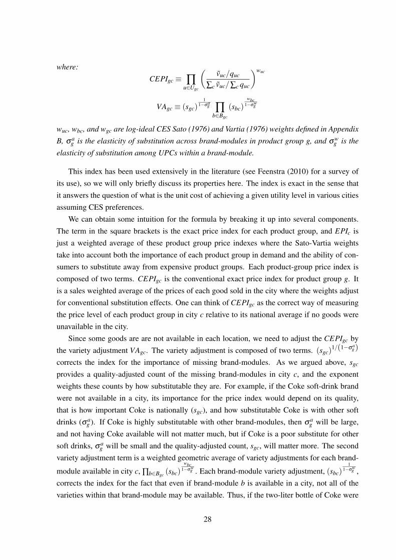
where:

CEPIgc ≡ ∏u∈Ugc

(vuc/quc

∑c vuc/∑c quc

)wuc

VAgc ≡ (sgc)1

1−σag ∏

b∈Bgc

(sbc)wbc

1−σwg

wuc, wbc, and wgc are log-ideal CES Sato (1976) and Vartia (1976) weights defined in Appendix

B, σag is the elasticity of substitution across brand-modules in product group g, and σw

g is the

elasticity of substitution among UPCs within a brand-module.

This index has been used extensively in the literature (see Feenstra (2010) for a survey ofits use), so we will only briefly discuss its properties here. The index is exact in the sense thatit answers the question of what is the unit cost of achieving a given utility level in various citiesassuming CES preferences.

We can obtain some intuition for the formula by breaking it up into several components.The term in the square brackets is the exact price index for each product group, and EPIc isjust a weighted average of these product group price indexes where the Sato-Vartia weightstake into account both the importance of each product group in demand and the ability of con-sumers to substitute away from expensive product groups. Each product-group price index iscomposed of two terms. CEPIgc is the conventional exact price index for product group g. Itis a sales weighted average of the prices of each good sold in the city where the weights adjustfor conventional substitution effects. One can think of CEPIgc as the correct way of measuringthe price level of each product group in city c relative to its national average if no goods wereunavailable in the city.

Since some goods are are not available in each location, we need to adjust the CEPIgc bythe variety adjustment VAgc. The variety adjustment is composed of two terms. (sgc)

1/(1−σag )

corrects the index for the importance of missing brand-modules. As we argued above, sgc

provides a quality-adjusted count of the missing brand-modules in city c, and the exponentweights these counts by how substitutable they are. For example, if the Coke soft-drink brandwere not available in a city, its importance for the price index would depend on its quality,that is how important Coke is nationally (sgc), and how substitutable Coke is with other softdrinks (σa

g ). If Coke is highly substitutable with other brand-modules, then σag will be large,

and not having Coke available will not matter much, but if Coke is a poor substitute for othersoft drinks, σa

g will be small and the quality-adjusted count, sgc, will matter more. The secondvariety adjustment term is a weighted geometric average of variety adjustments for each brand-

module available in city c, ∏b∈Bgc (sbc)wbc

1−σwg . Each brand-module variety adjustment, (sbc)

11−σw

g ,corrects the index for the fact that even if brand-module b is available in a city, not all of thevarieties within that brand-module may be available. Thus, if the two-liter bottle of Coke were

28

not available in a city, the impact on the price index would depend on how important two-liter Coke is (sbc) and how similar two-liter Coke is to other Coke products (σw

g ). We obtain theelasticities of substitution computed for UPCs within a brand-module and across brand-moduleswithin a product group from Broda and Weinstein (2010).

5.2 Measuring the Share of Commonly Available Goods

Recall that we do not observe the full set of UPCs available in each city. Just as we estimated theraw count of UPCs available in each city, we now have to estimate the quality-adjusted counts(or national expenditure shares) of available brand-modules (sgc) and UPCs (sbc). In Section4.2, we built an accumulation curve corresponding to the raw count of the UPCs representedin different-sized samples of households for each city. We now use the same method to buildcurves corresponding to the national market shares of the different brand-modules and UPCsrepresented in a sample. Our estimates of the sgc and sbc are simply the asymptotes of theseshares accumulation curves in each market. If sgc(n) denotes the national expenditure shareof brand-modules within a product group g purchased by n households in city c, our estimateof sgc (the national market share of the brand-modules that are available in a city within aproduct group) is simply the value we expect sgc (n) to take when the number of householdsequals the number of households in the city, which we approximate using the asymptote ofthe accumulation curve, or limn→∞ sgc(n). We use a similar procedure to estimate the nationalmarket share of the UPCs that are available in a city within each brand-module that is availablein the city, sbc.

Unfortunately, we are unable to estimate a value of sbc for every brand-module b in eachproduct group g for each city c because household samples are sometimes too small to allowus to observe more than a few purchases of UPCs within many of the brand-modules availablein a city. Since we do not want to estimate accumulation curves for brand-modules in whichthere are very few purchases, we pool the data across brand-modules in each city and estimatea common sbc within each product group, which we denote sgc. In other words, sgc tells tellsus the average national market share of UPCs available in a city within the set available brand-modules in a product group in that city. Since sgc does not vary at the brand-module level, thisassumption simplifies the variety adjustment in Proposition 1 to:

VAgc ≡ (sgc)1

1−σag (sgc)

11−σw

g (7)

5.3 Price Level in Cities: Evidence

In this section we will present our variety-adjusted exact prices for each city. First, however, weillustrate how we estimate the brand-module and UPC share inputs into the variety-adjustment

29

component (sgc and sgc) using the bread product group and show how these quality-adjustedcounts vary across cities of different sizes.

Figures 8 and 9 plot the share accumulation curves for one of the largest product groupsin terms of sales and the number of varieties available nationally (bread and baked goods) andusing data from two cities with very different populations, New York and Des Moines. Figure 8shows the sgc accumulation curve, which tells us about the availability of brand-modules, whileFigure 9 portrays the same curve for sgc (which tells us about the availability of UPCs withinbrand-modules). We estimate sgc and sgc for each product group and city as the asymptotes ofa Weibull function fitted to each of these curves. As one can see from the plots, the Weibull fitsthe share accumulation curves extremely well.30 By examining the asymptote of the Weibulldistribution in the first panel, we can see that New Yorkers have access to a set of bread brand-modules available that constitute 80 percent of national expenditures on bread. By contrast,residents of Des Moines, with a population less than a fortieth as large, have access to breadbrand-modules that constitute only 62 percent of national expenditures. In other words, thequality-adjusted count of brand-module varieties is higher in Des Moines than in New York.

Figure 9 shows that even when brand-modules are available in a city, many of the UPCs thatmake up these brand-modules are often not available. For example, consumers in New York andDes Moines only had access to bread UPCs that accounted for on average 64 and 43 percentof their brands’ national sales in a given module, respectively. This indicates that knowing thata firm sells a product in a city does not necessarily mean that all varieties of that product areavailable there.

In summary, the bread brand-modules available to New Yorkers account for 18 percent moreof the national bread market than the brand-modules available in Des Moines and, conditionalon a brand being available in their city, the varieties of these brand-modules available to NewYorkers account for 21 percent more of the national market for each brand-module than thevarieties of these brand-modules available to Des Moines residents.

To demonstrate how these differences in the market shares of UPCs and brand-modulesavailable in the two cities translate into a discount on the exact price index in New York relativeto Des Moines, we can calculate the variety adjustments for bread in each city from equation (7).The elasticity of substitution between UPCs within brand-modules in the bread product groupis 17.2, so the UPC variety adjustment for New York is 0.641/(1−17.2), or 1.028. The across-brand-module elasticity of substitution for the bread product group is 9.6, so the brand-modulevariety adjustment for New York is 0.801/(1−9.6), or 1.026. Assuming that that all availablegoods are sold at the same price in all locations, our estimates imply that the fact that there arefewer bread varieties available in New York than nationally means that someone restricted to

30We selected the Weibull since the AIC favored it for the raw count accumulation curves. We find that the AICfavors the Weibull distribution when estimating the share accumulation curves as well.

30

Figure 8: Brand-Module Share Accumulation Curves for the Bread Product Group

.2.4

.6.8

Bra

nd S

hare

0 1000 2000 3000Number of households

Accumulation Curve Fitted Weibull

Weibull Asymptote

New York: y = .8 * [1−exp(−.48 x^.29)]

.2.4

.6.8

0 1000 2000 3000Number of households

Accumulation Curve Fitted Weibull

Weibull Asymptote

Des Moines: y = .62 * [1−exp(−.38 x^.47)]

Figure 9: UPC Share Accumulation Curves for the Bread Product Group

0.2

.4.6

UPC

Sha

re

0 1000 2000 3000Number of households

Accumulation Curve Fitted Weibull

Weibull Asymptote

New York: y = .64 * [1−exp(−.12 x^.45)]

0.2

.4.6

0 1000 2000 3000Number of households

Accumulation Curve Fitted Weibull

Weibull Asymptote

Des Moines: y = .43 * [1−exp(−.05 x^.76)]

31

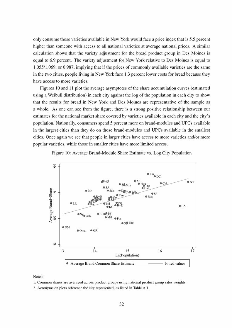
only consume those varieties available in New York would face a price index that is 5.5 percenthigher than someone with access to all national varieties at average national prices. A similarcalculation shows that the variety adjustment for the bread product group in Des Moines isequal to 6.9 percent. The variety adjustment for New York relative to Des Moines is equal to1.055/1.069, or 0.987, implying that if the prices of commonly available varieties are the samein the two cities, people living in New York face 1.3 percent lower costs for bread because theyhave access to more varieties.

Figures 10 and 11 plot the average asymptotes of the share accumulation curves (estimatedusing a Weibull distribution) in each city against the log of the population in each city to showthat the results for bread in New York and Des Moines are representative of the sample asa whole. As one can see from the figure, there is a strong positive relationship between ourestimates for the national market share covered by varieties available in each city and the city’spopulation. Nationally, consumers spend 5 percent more on brand-modules and UPCs availablein the largest cities than they do on those brand-modules and UPCs available in the smallestcities. Once again we see that people in larger cities have access to more varieties and/or morepopular varieties, while those in smaller cities have more limited access.

Figure 10: Average Brand-Module Share Estimate vs. Log City Population

DM

LR

Oma

Syr Alb

Bir

RicLou

GR

JacMemR−DNas

SLC

ChaCol

SA

Ind

OrlMilNH

KC

Sac

NOOkCCin

Por

B−RPit

TamDen

StL

SD

Cle

Min

Pho

SeaMia

AtlHou

DalDet

Bos

Phi

SF

DC

Chi

LA

NY

.8.8

5.9

.95

Ave

rage

Bra

nd−S

hare

13 14 15 16 17Ln(Population)

Average Brand Common Share Estimate Fitted values

Notes:1. Common shares are averaged across product groups using national product group sales weights.2. Acronyms on plots reference the city represented, as listed in Table A.1.

32

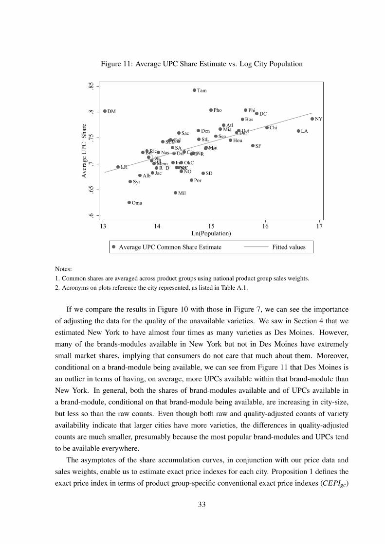
Figure 11: Average UPC Share Estimate vs. Log City Population

DM

LR

Oma

SyrAlb

BirRicLou

GR

Jac

MemR−D

Nas

SLCChaColSA

Ind

Orl

Mil

NHKC

Sac

NO

OkC

Cin

Por

B−RPit

Tam

Den

StL

SD

CleMin

Pho

SeaMia

Atl

HouDalDet

Bos

Phi

SF

DC

Chi LA

NY

.6.6

5.7

.75

.8.8

5A

vera

ge U

PC−S

hare

13 14 15 16 17Ln(Population)

Average UPC Common Share Estimate Fitted values

Notes:1. Common shares are averaged across product groups using national product group sales weights.2. Acronyms on plots reference the city represented, as listed in Table A.1.

If we compare the results in Figure 10 with those in Figure 7, we can see the importanceof adjusting the data for the quality of the unavailable varieties. We saw in Section 4 that weestimated New York to have almost four times as many varieties as Des Moines. However,many of the brands-modules available in New York but not in Des Moines have extremelysmall market shares, implying that consumers do not care that much about them. Moreover,conditional on a brand-module being available, we can see from Figure 11 that Des Moines isan outlier in terms of having, on average, more UPCs available within that brand-module thanNew York. In general, both the shares of brand-modules available and of UPCs available ina brand-module, conditional on that brand-module being available, are increasing in city-size,but less so than the raw counts. Even though both raw and quality-adjusted counts of varietyavailability indicate that larger cities have more varieties, the differences in quality-adjustedcounts are much smaller, presumably because the most popular brand-modules and UPCs tendto be available everywhere.

The asymptotes of the share accumulation curves, in conjunction with our price data andsales weights, enable us to estimate exact price indexes for each city. Proposition 1 defines theexact price index in terms of product group-specific conventional exact price indexes (CEPIgc)

33

and variety adjustments (VAgc). We aggregate across product groups to obtain values for eachof these components for each city. Rearranging terms in the exact price index definition fromProposition 1, we can see that the exact price index is the product of each of these aggregatecomponents:

EPIc = ∏g∈G

[CEPIgcVAgc]wgc = ∏

g∈G[CEPIgc]

wgc∏g∈G

[VAgc]wgc =CEPIcVAc.

Table 6 presents our estimates for how the conventional exact price index (CEPIc), the varietyadjustment (VAc), and their product, the exact price index (EPIc), vary across cities. The firstthree columns in the table use unadjusted prices to compute the index. As we saw in Table2, unadjusted prices are higher in larger cities, and these results translate into a common exactprice index that rises with city size. These higher prices, however, are offset by an even strongervariety adjustment to prices arising from the greater availability of varieties in larger cities,leading to an exact price index that falls slightly, but not significantly with city size.

Table 6: Are price indexes higher in larger cities?

Unadjusted Prices Prices Adjusted for Prices Adjusted forPurchaser Heterogeneity Purchaser and Store Heterogeneity

CEPIc VAc EPIc CEPIc VAc EPIc CEPIc VAc EPIc

[1] [2] [3] [4] [5] [6] [7] [8] [9]Ln(Populationc) 0.012*** -0.016*** -0.0025 0.012*** -0.016*** -0.003 0.0041** -0.015*** -0.011***

[0.0035] [0.0028] [0.0050] [0.0034] [0.0028] [0.0050] [0.0018] [0.0028] [0.0036]Constant 0.82*** 1.31*** 1.11*** 0.82*** 1.31*** 1.12*** 0.94*** 1.31*** 1.24***

[0.051] [0.042] [0.074] [0.050] [0.042] [0.073] [0.027] [0.042] [0.053]

Observations 49 49 49 49 49 49 49 49 49R-squared 0.206 0.394 0.005 0.201 0.394 0.007 0.096 0.388 0.167

Standard errors in brackets; *** p<0.01, ** p<0.05, * p<0.1.

Notes:1. The dependent variables in the above regressions are indices. These indices are calculated using unadjusted prices or prices that have beenadjusted as indicated above, using estimates from the regression in Column [4] of Panel A in Table 2.2. EPIc = CEPIcVAc which implies that log(EPIc) = log(CEPIc) + log(VAc). Note that the dependent variables in theabove regressions are in levels, not logs, so the coefficients on log population in the CEPIc and VAc regressions do not add to thecoefficient on log population in the EPIc regression.

As we argued in Section 3.3, the unadjusted prices, however, are problematic because theydo not correct for the store in which the goods are purchased or the type of household making thepurchase. We therefore use adjusted prices in the subsequent columns. Our price adjustmentsare based on the estimates from Column 4 of Table 2. Adjusting for purchaser heterogeneityhardly had any impact in Table 2, and it barely affects our point estimates in columns 4-6.However, adjusting for retailer heterogeneity has a big impact. Columns 7-9 present resultsin which we also control for retailer heterogeneity. We still obtain a statistically significantpositive association between city size and the common goods price index, but it is economicallysmall in size. A person moving from Des Moines to New York City would experience the price

34

Figure 12: City Price Indexes vs. Log City Population

Indexes Calculated using Unadjusted Prices

LROmaSyr BirRic

Lou

JacMem

R−D

NasSLC

Cha

Col

SA

Ind

OrlMil

NH

KC

Sac

OkCCin

PorB−R

PitTam

Den

StL

SD

Cle

Min

Pho

SeaMia

Atl

Hou

DalDet

BosPhi

SF

DCChi

LA NY

−.08

−.04

0.0

4.0

8ce

pi

13 14 15 16 17Ln(Population)

LR

Oma

Syr

BirRic

Lou

JacMem

R−D

NasSLC

Cha

Col

SA

IndOrl

MilNH

KC

Sac

OkCCin

Por

B−R

Pit

Tam

DenStL

SD

Cle

Min

Pho

Sea

Mia

AtlHou

DalDetBosPhi

SF

DC

Chi

LA

NY

−.08

−.04

0.0

4.0

8ep

i

13 14 15 16 17Ln(Population)

Indexes Calculated using PricesAdjusted for Purchaser and Store Heterogeneity

LR

OmaSyrBirRic

LouJacMemR−DNas

SLC

ChaColSAIndOrlMilNHKC

Sac

OkCCinPorB−RPitTamDen

StL

SD

CleMin

PhoSea

Mia

AtlHou

Dal

DetBosPhi

SF

DCChi

LA NY

−.08

−.04

0.0

4.0

8ce

pi

13 14 15 16 17Ln(Population)

LR

Oma

Syr

BirRic

Lou

JacMemR−D

Nas

SLCChaColSA

IndOrl

MilNHKCSac

OkCCin

Por

B−R

Pit

Tam

DenStL

SD

Cle

Min

Pho

Sea

MiaAtlHouDal

Det

BosPhi

SF

DC Chi

LA

NY

−.08

−.04

0.0

4.0

8ep

i

13 14 15 16 17Ln(Population)

Notes:1. Acronyms on plots reference the city represented, as listed in Table A.1.2. City price indexes are normalized to be mean zero.

of commonly available groceries rise by 1.5 percent. However, this higher common goods priceindex would be more than offset by the fact that many goods are not available in Des Moinesand are therefore effectively priced at their reservation level. The gains due to variety mean thatthe theoretically rigorous exact price index indicates that the price level in New York is actually4.2 percent lower than Des Moines.

We can assess the importance of the heterogeneity and variety availability biases visuallyin Figure 12. The plots on the left shows how the common-goods exact price index variesacross cities, and the plots on the right shows how the variety-adjusted exact price index varies.As we saw in Figure 2, there is virtually no upward relationship between the price index forcommonly available UPCs that adjusts for heterogeneity biases and only a slight upward sloping

35

relationship when we do not. Similarly, the negative relationship between city population andthe variety-adjusted exact price index is clearly not driven by any outliers.

Figure 12 also demonstrates how controlling for heterogeneity impacts the variance of theprice level across cities. The common-goods exact price indexes plotted on the top left arecalculated with unadjusted prices. The variance in these price indexes, that control for productheterogeneity but not purchaser or store effects, is already 87 percent lower than the variance inour replication of the ACCRA food price index. When we further control for purchaser and storeheterogeneity in the indexes on plotted on the bottom left, the variance falls by an additional10 percentage points to just 3 percent of the variance in the ACCRA-style index. In sum, thevariance in the price level falls by 97 percent when we move from an ad hoc price index toa theoretically-justified one that corrects for both heterogeneity and substitution biases. Thisdrop is almost identical to the 95 percent decline in variance that we observed comparing ourreplication of the ACCRA food price index with the city fixed effects estimated in Section 5.3.The methodological differences between the city fixed effects and the CES indexes, therefore,play only a small role in the drop in variance. We attribute most of the variance in measuredPPP of commonly-available food products to heterogeneity, rather than substitution biases.31

It is interesting to compare the common-good exact price index, CEPIc, in Table 6, withthe coefficient on the city fixed effects, αc, in Table 2. We can think of the city fixed effectsas a price index in the sense that they summarize the relative price levels across locations,where relative prices are weighted by the transaction value weights used in the regressions.An important difference between the two is that the Sato-Vartia weights used to calculate theCEPIc are theoretically justified if one assumes a CES utility function, whereas the transactionweights used in the estimation of the αc’s do not have a theoretical justification but rather servean econometric purpose: to minimize the influence of errors associated with small transactionson the estimates. Nevertheless, it is reassuring that the associations between these variablesand population are so close; the differences are typically around 0.002. This indicates that ourresults regarding the computation of the price level of available goods in a city are robust to anumber of sensible aggregation methods.

Taken together with those in Section 3, these results suggest that conventional price indexesprovide a very misleading picture of what the prices of tradables are in cities and also help toexplain why. In Column 1 of Table 1, we saw that the elasticity of a conventional urban priceindex with respect to population was 4.2 percent. However, once we controlled for productheterogeneity, the fact that the standard urban price indexes don’t compare the same goods,we see that the elasticity falls to 1.6 percent (Column 1 of Table 2): a loss of two-thirds of itsmagnitude. Controlling for purchaser and especially retailer heterogeneity more than halves themagnitude of this coefficient, taking it down to 0.6 percent. Further using the common exact

31These price indexes and their relative variances are listed in Appendix Table (A.2).

36

price index instead of an ad hoc one, which is the principle difference between CEPIc and αc,reduces the coefficient to 0.4 percent (Column 7 of Table 6), which is less than on tenth of itsinitial magnitude. Finally, the exact price index, which differs from the CEPIc by correcting forthe fact that some goods are dropped from CEPIc because they are not available (an extremeform of substitution bias), flips the sign, suggesting that the elasticity of urban price with respectto population is -1.1 percent (Column 9 of Table 6): a 5 percentage point differential. Thus, thestandard result that the prices of tradables are higher in cities is due to a series of measurementissues. If one uses a theoretically-sound approach, the result reverses.

5.4 Robustness

One possible concern about these results is that people who live in large cities might not shopin all of the neighborhoods within the city’s borders. This might bias our variety adjustmentdownwards because we may be counting varieties in, say, suburbs that are irrelevant for peoplewho live downtown.

An easy solution to this problem is to make use of the fact that the Nielsen data records thehousehold’s county and the zip codes of the stores in which they purchase each UPC. We firstassume that a household is located in the zip code in the county where its grocery expendituresare the highest. We then construct the population of the market where households in each zipcode can choose to shop. For a set of households living in the same zip code, we sum thepopulations of the zip codes where we observe the set of households purchasing UPCs. Thissum tells us the population of the market that is available to households located in that zip code.We average these market populations across the zip codes in each city to yield the averagepopulation of the neighborhoods where households in the city choose to shop. We refer to thisnumber as the relevant population.

Table 7 presents results in which we replace the city’s population with the relevant popu-lation in the neighborhoods in which households actually shop. The results are, if anything,stronger than the results using urban population as the measure of city size. The fact that theresults are so similar indicates that understanding where households shop within cities is notimportant for understanding the relationship between city size and prices. The key finding isthat the exact price index falls with city size, and this relationship is significant whenever weadjust prices to take into account store amenities and buyer characteristics.

6 Producer Prices in Cities

Thus, far we have been focused on consumer prices. However, given that we did not findmuch variation in retail markups (which is consistent with our CES structure), we push the

37

Table 7: Are price indexes higher in larger markets?

Unadjusted Prices Prices Adjusted for Prices Adjusted for PurchaserPurchaser Heterogeneity and Store Heterogeneity

CEPIc VAc EPIc CEPIc VAc EPIc CEPIc VAc EPIc

[1] [2] [3] [4] [5] [6] [7] [8] [9]Ln(Relevant 0.0082*** -0.016*** -0.0066 0.0079** -0.016*** -0.0069* 0.0027* -0.015*** -0.012***Populationc) [0.0030] [0.0020] [0.0041] [0.0030] [0.0020] [0.0040] [0.0016] [0.0020] [0.0027]Constant 0.86*** 1.34*** 1.18*** 0.86*** 1.34*** 1.19*** 0.95*** 1.34*** 1.29***

[0.050] [0.034] [0.068] [0.049] [0.034] [0.067] [0.026] [0.034] [0.045]Observations 49 49 49 49 49 49 49 49 49R-squared 0.137 0.553 0.052 0.133 0.553 0.058 0.06 0.549 0.304

Standard errors in brackets; *** p<0.01, ** p<0.05, * p<0.1

Notes:1. The dependent variables in the above regressions are indices. These indices are calculated using unadjusted prices or prices that have beenadjusted as indicated above, using estimates from the regression in Column [4] of Panel A in Table 2.2. EPIc = CEPIcVAc which implies that log(EPIc) = log(CEPIc) + log(VAc). Note that the dependent variables in theabove regressions are in levels, not logs, so the coefficients on log population in the CEPIc and VAc regressions do not add to thecoefficient on log population in the EPIc regression.

data and strip prices of retailing costs to estimate how producer prices vary across cities. Thisis an interesting exercise because many economic geography models (e.g., Helpman (1998))postulate that the price index for tradables should be lower in larger cities, and the price of landoffsets this price. In these models, it might be the case that producer prices are lower in largercities, even when consumer prices indexes, which include land costs, are not.32 Land costsmay drive a similar wedge between retail and wholesale prices in our data. Our retail pricesundoubtedly contain a non-traded land component reflecting the rent paid by the stores sellingthe goods. The fact that we observe PPP in these retail prices does not rule out the possibilitythat producer prices are lower in bigger cities. While our results provide the correct elasticitybetween consumer prices and the size of a city, to the extent that rents are higher in largercities, they likely understate the relationship between the prices of traded goods and city size.Although it is not appropriate for welfare analysis, it is worth considering what happens to thetraded component of goods prices as city size varies.

If we assume that all prices contain a non-traded rental component that rises in proportion tothe rent, we can examine how the tradable component of the price index moves with populationby controlling for a city’s commercial real estate rental cost in the price regressions. This effectis easiest to see in comparing Panels A and B of Table 8. Panel A replicates the price-city sizeregressions across the 45 cities for which we have retail rent data. These results are almostidentical to the estimates over the full sample: each of the coefficients and their associatedstandard errors are identical to their corresponding values in Panel B in Table 2 up to onesignificant figure. In Panel B, we include retail rents as an explanatory variable and estimate

32In Helpman (1998), producer prices of identical tradable goods are lower, on average, in larger cities becausemore goods are produced in high population areas and these goods can be consumed locally without paying trans-port costs. There could, however, be other mechanisms driving our results here. We leave distinguishing betweenthese explanations to future work.

38

αc = α + γ ln(Popc)+δ ln(Rentc)+ εc, (8)

where ln(Rentc) is the log of commercial real estate rents in city c and greek letters are pa-rameters to be estimated. The results indicate a very strong positive relationship between retailrents and urban price levels as is evidenced by the large positive and significant coefficient onlog retail rents and the dramatic jump in R2. Once again, the coefficient on population now be-comes negative (although not significantly so), indicating a weak negative association betweencity size and the prices of traded goods. Interestingly, the coefficient on retail rent is quite smallin most specifications, which suggests that the elasticity of goods prices with respect to retailrents is less than 10 percent. This helps explain why the deviations from PPP are so small infigures 2 and 12.33

We also can adjust our price index regressions in Table 6 for this force. In Panel B of Table9, we regress each element of our exact price index on both log population and log rent. As onemight expect, controlling for land rents has a big impact on the common-good exact price indexbut has almost no impact on the variety-adjustment, which has no clear theoretical tie to landprices. Overall, this suggests that the price index for the tradable component of goods pricesfalls about 50 percent faster than the overall index.

Although there is a weak positive relationship between city size and retail prices after con-trolling for product, purchaser, and retailer heterogeneity (but not product availability), theseresults suggest that this positive association is entirely due to the fact that retail prices incorpo-rate non-traded goods prices, which vary across cities: if we focused on wholesale prices alone,we would expect to see, if anything, a negative association with city size.

7 Conclusion

In this paper we have shown how the lack of sophistication of standard spatial price indexes canlead to very misleading portraits of how prices vary across space. We find that most of the largedispersion in food prices across space can be attributed problems in the measurement of theseprices. 97 percent of the variation in price levels across space in these indexes can be attributedto unobserved heterogeneity in the goods being compared. In particular, product and retailerheterogeneity play very large roles. We also show that standard indexes suffer severely from thespatial equivalent of the “new goods bias” that is well known in inflation measurement. Smallcities offer consumers a much smaller array of available goods. Building a price index that

33This result is robust across all of our specifications from Section 3. We have replicated the results in Tables3 and 4 over the sample of cities with retail rents data and find almost no change in the coefficients and theirstatistical significance. In all cases, adding retail rents to these regressions flips the sign on the coefficient onpopulation (although the point estimate is no-longer significant).

39

Table 8: Prices and City Size, Controlling for Rents

City Fixed Effect Coefficient from Panel A of Table 2

[1] [2] [3] [4]UPC Fixed Effects Yes Yes Yes YesCity Fixed Effects Yes Yes Yes YesHousehold Demographic Dummies No Yes No YesStore Dummies No No Yes Yes

Panel A: Cities with Non-Missing Retail Rent Data

Ln(Populationc) 0.0133*** 0.0123*** 0.00649*** 0.00610**[0.00437] [0.00433] [0.00237] [0.00236]

Constant -0.235*** -0.218*** -0.124*** -0.117***[0.0644] [0.0637] [0.0350] [0.0348]

Observations 45 45 45 45R-Squared 0.177 0.159 0.148 0.134

Panel B: Controlling for Retail Rents

Ln(Populationc) -0.00648 -0.00725* -0.00236 -0.00279[0.00421] [0.00416] [0.00266] [0.00263]

Ln(Retail Rentc) 0.101*** 0.0996*** 0.0450*** 0.0452***[0.0148] [0.0146] [0.00932] [0.00923]

Constant -0.216*** -0.199*** -0.115*** -0.108***[0.0451] [0.0445] [0.0284] [0.0282]

Observations1 45 45 45 45R-Squared 0.608 0.601 0.452 0.449

Standard errors in brackets; *** p<0.01, ** p<0.05, * p<0.1

Notes:1. Sample is limited to the 45 markets for which commercial retail rent data was available.

takes all of these biases into account, we reverse the conventional finding that tradable goodsprices rise with city size. The elasticity of tradable goods prices with respect to city populationis -0.11.

These results have important implications for a broad class of New Economic Geographymodels in which agglomeration is driven, at least in part, by pecuniary externalities. In Krugman(1991)’s model of monopolistic competition, these externalities arise when there are positivetrade costs between locations: locally-produced goods are cheaper in the local market than theyare elsewhere and larger cities produce more varieties than smaller ones, so consumers in theselocations have access to more locally-produced goods and therefore face a lower price index.

More recent papers propose that other mechanisms are at play here. Behrens and Robert-Nicoud (2011) and Combes et al. (2012) demonstrate that, with quadratic linear preferencesand fixed trade costs as in Melitz and Ottaviano (2008), three related phenomena yield lowerprices in larger cities: (i) more efficient firms are more likely to locate in, or “select into,”

40

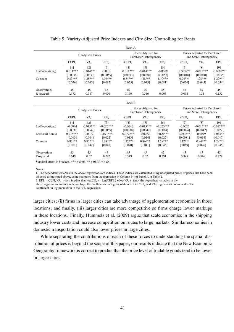
Table 9: Variety-Adjusted Price Indexes and City Size, Controlling for Rents

Panel A

Unadjusted Prices Prices Adjusted for Prices Adjusted for PurchaserPurchaser Heterogeneity and Store Heterogeneity

CEPIc VAc EPIc CEPIc VAc EPIc CEPIc VAc EPIc

[1] [2] [3] [4] [5] [6] [7] [8] [9]Ln(Populationc) 0.011*** -0.014*** -0.0013 0.011*** -0.014*** -0.0019 0.0038** -0.013*** -0.0093**

[0.0038] [0.0030] [0.0055] [0.0037] [0.0030] [0.0055] [0.0018] [0.0030] [0.0036]Constant 0.83*** 1.28*** 1.09*** 0.84*** 1.28*** 1.10*** 0.94*** 1.28*** 1.22***

[0.056] [0.045] [0.082] [0.055] [0.045] [0.081] [0.026] [0.045] [0.054]

Observations 45 45 45 45 45 45 45 45 45R-squared 0.172 0.317 0.001 0.160 0.316 0.003 0.094 0.31 0.132

Panel B

Unadjusted Prices Prices Adjusted for Prices Adjusted for PurchaserPurchaser Heterogeneity and Store Heterogeneity

CEPIc VAc EPIc CEPIc VAc EPIc CEPIc VAc EPIc

[1] [2] [3] [4] [5] [6] [7] [8] [9]Ln(Populationc) -0.0044 -0.015*** -0.020*** -0.0046 -0.015*** -0.020*** -0.0023 -0.015*** -0.017***

[0.0039] [0.0042] [0.0065] [0.0038] [0.0042] [0.0064] [0.0024] [0.0042] [0.0050]Ln(Retail Rentc) 0.078*** 0.0072 0.091*** 0.077*** 0.0072 0.090*** 0.033*** 0.0079 0.043**

[0.013] [0.014] [0.022] [0.013] [0.014] [0.022] [0.0081] [0.014] [0.017]Constant 0.82*** 0.85*** 1.28*** 1.12*** 0.86*** 1.28*** 1.12*** 0.94*** 1.28***

[0.051] [0.042] [0.045] [0.070] [0.041] [0.045] [0.069] [0.026] [0.045]

Observations 45 45 45 45 45 45 45 45 45R-squared 0.549 0.32 0.292 0.549 0.32 0.291 0.348 0.316 0.228

Standard errors in brackets; *** p<0.01, ** p<0.05, * p<0.1

Notes:1. The dependent variables in the above regressions are indices. These indices are calculated using unadjusted prices or prices that have beenadjusted as indicated above, using estimates from the regression in Column [4] of Panel A in Table 2.2. EPIc = CEPIcVAc which implies that log(EPIc) = log(CEPIc) + log(VAc). Since the dependent variables in theabove regressions are in levels, not logs, the coefficients on log population in the CEPIc and VAc regressions do not add to thecoefficient on log population in the EPIc regression.

larger cities; (ii) firms in larger cities can take advantage of agglomeration economies in thoselocations; and finally, (iii) larger cities are more competitive so firms charge lower markupsin these locations. Finally, Hummels et al. (2009) argue that scale economies in the shippingindustry lower costs and increase competition on routes to large markets. Similar economies indomestic transportation could also lower prices in large cities.

While separating the contributions of each of these forces to understanding the spatial dis-tribution of prices is beyond the scope of this paper, our results indicate that the New EconomicGeography framework is correct to predict that the price level of tradable goods tend to be lowerin larger cities.

41

References

Albouy, David, “The Unequal Geographic Burden of Federal Taxation,” Journal of Political

Economy, 2009, 117 (41), 635–667.

Anderson, Simon P., Andre de Palma, and Jacques-Francois Thisse, “The CES is a DiscreteChoice Model?,” Economics Letters, 1987, 24, 139–140.

Aten, Bettina, “Report on Interarea Price Levels,” Bureau of Economic Analysis Working Pa-

pers, November 2005.

Atkin, David and Dave Donaldson, “Who’s Getting Globalized? The Size and Nature ofIntranational Trade Costs,” Yale University and MIT, unpublished mimeo, 2012.

B., Figueroa-E. Aten and T. Martin, “Notes on Estimating the Multi-Year Regional PriceParities by 16 Expenditure Categories: 2005-2009,” Bureau of Economic Analysis Working

Papers, April 2012, (0071).

Behrens, Kristian and Frederic Robert-Nicoud, “Survival of the Fittest in Cities: Agglomer-ation, Selection, and Inequality,” CEPR Discussion Papers, February 2011, (7019).

Bernard, Andrew B., J. Bradford Jensen, Stephen J. Redding, and Peter K. Schott, “Firmsin International Trade,” The Journal of Economic Perspectives, 2007, 21 (3), pp. 105–130.

Broda, Christian and David E. Weinstein, “Product Creation and Destruction: Evidence andPrice Implications,” American Economic Review, 2010, 100, 691.

, Nuno Limão, and David E. Weinstein, “Optimal Tariffs and Market Power: The Evi-dence,” The American Economic Review, 2008, 98 (5), 2032–2065.

Burstein, Ariel and Gita Gopinath, “International Prices and Exchange Rates,” NBER Work-

ing Paper 18829, 2013.

and Nir Jaimovich, “Understanding Movements in Aggregate and Product-Level Real Ex-change Rates,” unpublished paper, UCLA and Stanford University, 2009.

Chevalier, Judith A., “Capital structure and product-market competition: Empirical evidencefrom the supermarket industry,” The American Economic Review, 1995, p. 415–435.

Colwell, Robert K. and Jonathan A. Coddington, “Estimating Terrestrial Biodiversiththrough Extrapolation,” Philosophical Transactions: Biological Sciences, July 1994, 345

(1311), 101–118.

42

Combes, Pierre-Philippe, Gilles Duranton, Laurent Gobillon, Diego Puga, and SébastienRoux, “The productivity advantages of large cities: Distinguishing agglomeration from firmselection,” Econometrica, 2012, 80 (6), 2543–2594.

Couture, Victor, “Valuing the Consumption Benefits of Urban Density,” 2013.

Crucini, Mario J. and Mototsugu Shintani, “Persistence in law of one price deviations: Evi-dence from micro-data,” Journal of Monetary Economics, 2008, 55 (3), 629–644.

DuMond, J. Michael, Barry T. Hirsch, and David A. Macpherson, “Wage DifferentialsAcross Labor Markets and Workers: Does Cost of Living Matter?,” Economic Inquiry, Octo-ber 1999, 37 (4), 577–598.

Eaton, Jonathan, Samuel Kortum, and Francis Kramarz, “An anatomy of internationaltrade: Evidence from French firms,” Econometrica, 2011, 79 (5), 1453–1498.

Ellickson, Paul B. and Sanjog Misra, “Supermarket pricing strategies,” Marketing Science,2008, 27 (5), 811–828.

Feenstra, Robert C., “New Product Varieties and the Measurement of International Prices,”The American Economic Review, 1994, 84 (1), 157–177.

, Product Variety and the Gains from International Trade, MIT Press, 2010.

and David E. Weinstein, “Globalization, Markups, and the U.S. Price Level,” NBER Work-

ing Paper 15749, Febraury 2010, 35.

, Robert Inklaar, and Marcel Timmer, “The Next Generation of the Penn World Table,”2012.

Fujita, Masahisa, “A Monopolistic Competition Model of Spatial Agglomeration,” Regional

Science and Urban Economics, 1988, 18, 87–124.

Gopinath, Gita, Pierre-Olivier Gourinchas, Chang-Tai Hsieh, and Nicholas Li, “Interna-tional prices, costs, and markup differences,” The American Economic Review, 2011, 101 (6),2450–2486.

Handbury, Jessie, “Are Poor Cities Cheap for Everyone? Non-Homotheticity and the Cost ofLiving Across U.S. Cities,” 2012.

Helpman, Elhanan, “The size of regions,” in Itzhak Zilcha David Pines, Efraim Sadka, ed.,Topics in Public Economics, Cambridge University Press, 1998, pp. 33–54.

43

Hummels, David and Peter J. Klenow, “The Variety and Quality of a Nation’s Exports,” The

American Economic Review, 2005, 95 (3), 704–723.

, Volodymyr Lugovskyy, and Alexandre Skiba, “The trade reducing effects of marketpower in international shipping,” Journal of Development Economics, 2009, 89 (1), 84–97.

Jimenez-Valverde, Alberto, Silvia Jimenez Mendoza, Jose Martin Cano, and Miguel L.Munguira, “Comparing relative model fit of several species-accumulation functions to localPapilionoidea and Hesperioidea butterfly inventories of Mediterranean habitats,” Biodiversity

and Conservation, 2006, 15, 163–176.

Krugman, Paul, “Increasing Returns and Economic Geography,” Journal of Political Econ-

omy, 1991, 99 (3), 483–499.

Landry, Anthony, “Borders and Big Macs,” Economics Letters, 2013.

Mao, Chang Xuan, Robert K. Colwell, and Jing Chang, “Interpolating, Extrapolating, andComparing Incidence-Based Species Accumulation Curves,” Ecology, 2004, 85 (2717-2727),433–441.

, , and , “Estimating the Species Accumulation Curve Using Mixtures,” Biometrics,2005, 61 (2), 433–441.

Melitz, Marc J. and Gianmarco I. P. Ottaviano, “Market Size, Trade, and Productivity,”Review of Economic Studies, January 2008, 75 (1), 295–316.

Moretti, Enrico, “Real Wage Inequality,” American Economic Journal: Applied Economics,2013, 5 (1), 65–103.

Ottaviano, Gianmarco I.P., Takatoshi Tabuchi, and Jacques-Francois Thisse, “Agglomera-tion and Trade Revisited„” International Economic Review, May 2002, 43 (2), 409–435.

Parsley, David C. and Shang-Jin Wei, “Convergence to the Law of One Price Without TradeBarriers or Currency Fluctuations,” The Quarterly Journal of Economics, 1996, 111 (4),1211–1236.

Rivera-Batiz, Francisco L., “Increasing Returns, Monopolistic Competition, and Agglomera-tion Economies in Consumption and Production,” Regional Science and Urban Economics,1988, 18, 125–153.

Sato, Kazuo, “The Ideal Log-Change Index Number,” The Review of Economics and Statistics,1976, 58 (2), 223–228.

44

Schiff, Nathan, “Cities and product variety,” University of British Columbia, 2012.

Simonovska, Ina, “Income Differences and Prices of Tradables,” UC Davis Working Paper,2010, No. 10-15.

Suedekum, Jens, “Agglomeration and Regional Costs of Living,” Journal of Regional Science,2006, 46 (3), 529–543.

Tabuchi, Takatoshi, “On Interregional Price Differentials,” The Japanese Economic Review,March 2001, 52 (1), 104–115.

Vartia, Y., “Ideal Log-Change Index Numbers,” Scandinavian Journal of Statistics, 1976, 3

(3), 121–126.

45

AppendicesTable A.1: Sample Market Data

EffectiveSample Retail Normalized

Population1 Household Rent3 HerfindahlMarket Name (thousands) Count2 (psf) Index4

Correlation with Population 0.20 0.54 0.00 0.18

Omaha (Oma) 717 116 11.70 0.116Jacksonville (Jac) 1,100 130 12.95 0.157Albany (Alb) 876 138 - 0.139San Diego (SD) 2,814 139 23.52 0.116Des Moines (DM) 456 145 - 0.176Syracuse (Syr) 732 164 10.77 0.078Milwaukee (Mil) 1,690 170 13.37 0.220Hartford-New Haven (NH) 1,725 193 14.53 0.138Richmond (Ric) 997 194 15.04 0.120Grand Rapids (GR) 1,089 198 - 0.221Kansas City (KC) 1,776 220 12.10 0.082Raleigh-Durham (R-D) 1,188 239 15.25 0.113Indianapolis (Ind) 1,607 245 12.82 0.109Orlando (Orl) 1,645 247 15.74 0.203Salt Lake City (SLC) 1,334 248 14.11 0.092Portland, Or (Por) 2,265 263 16.76 0.110Pittsburgh (Pit) 2,359 303 14.07 0.143Cincinnati (Cin) 1,979 317 12.52 0.201Memphis (Mem) 1,136 331 11.98 0.155Little Rock (LR) 584 351 11.11 0.193Cleveland (Cle) 2,946 362 13.88 0.095Nashville (Nas) 1,231 403 12.99 0.169New Orleans-Mobile (NO) 1,878 409 - 0.216Louisville (Lou) 1,026 454 13.46 0.209Oklahoma City-Tulsa (OkC) 1,887 528 9.83 0.147Birmingham (Bir) 921 570 12.81 0.154Dallas (Dal) 5,222 899 14.05 0.119San Antonio (SA) 1,592 921 12.48 0.305San Francisco (SF) 7,039 995 29.90 0.152Detroit (Det) 5,456 1,001 15.66 0.135Atlanta (Atl) 4,112 1,038 15.31 0.141Sacramento (Sac) 1,797 1,052 19.84 0.064Chicago (Chi) 9,158 1,064 16.92 0.127Houston (Hou) 4,670 1,070 13.63 0.143Miami (Mia) 3,876 1,086 20.08 0.286Columbus (Col) 1,540 1,101 10.97 0.171Charlotte (Cha) 1,499 1,115 14.89 0.132Washington, DC-Baltimore (DC) 7,608 1,115 21.49 0.070Denver (Den) 2,582 1,128 14.70 0.163Buffalo-Rochester (B-R) 2,268 1,135 11.20 0.176Seattle (Sea) 3,555 1,149 19.78 0.104Los Angeles (LA) 16,400 1,151 24.47 0.100Tampa (Tam) 2,396 1,173 13.11 0.198St. Louis (StL) 2,604 1,183 12.84 0.107Philadelphia (Phi) 6,188 1,183 17.02 0.066Phoenix (Pho) 3,252 1,211 16.27 0.129Minneapolis (Min) 2,969 1,236 14.99 0.165Boston (Bos) 5,819 1,275 19.03 0.122New York (NY) 21,200 1,477 20.13 0.088

Sources and notes:1. 2000 U.S. Census.2. 2005 Nielsen HomeScan sample.3. 2005 Community/Neighborhood Shopping Center Effective Rents from reis.com.4. Herfindahl indexes measure the concentration of retail chains in each market.

46

Table A.2: Price Indexes

Price Indexes2

Nielsen Unadjusted Purchaser-Store AdjustedPopulation1 Food City Fixed City Fixed

Market Name (thousands) Index3 Effect4 CEPI6 Effect4 CEPI6 EPI6

Correlation with Population 1.00 0.49 0.44 0.43 0.42 0.37 -0.19Coefficient of Variation 6.8% 2.6% 2.2% 1.3% 1.1% 2.0%Var(Index)/Var(Nielsen Food Index) 0.18 0.13 0.05 0.03 0.12

Omaha (Oma) 717 0.802 0.959 0.968 0.963 0.971 1.039Jacksonville (Jac) 1,100 0.872 0.953 0.961 0.969 0.976 1.007Albany (Alb) 876 0.924 0.967 0.970 0.973 0.975 1.013San Diego (SD) 2,814 0.973 1.004 1.001 0.996 0.995 1.033Des Moines (DM) 456 0.844 0.927 0.940 0.964 0.974 1.039Syracuse (Syr) 732 0.847 0.953 0.961 0.967 0.972 1.014Milwaukee (Mil) 1,690 0.871 0.969 0.980 0.955 0.965 1.015Hartford-New Haven (NH) 1,725 0.976 0.998 0.998 0.987 0.985 1.019Richmond (Ric) 997 0.849 0.954 0.963 0.976 0.983 1.007Grand Rapids (GR) 1,089 0.833 0.930 0.938 0.978 0.981 1.016Kansas City (KC) 1,776 0.840 0.953 0.962 0.975 0.980 1.014Raleigh-Durham (R-D) 1,188 0.905 0.972 0.981 0.968 0.977 1.003Indianapolis (Ind) 1,607 0.836 0.945 0.955 0.964 0.972 1.000Orlando (Orl) 1,645 0.907 0.961 0.970 0.971 0.975 0.985Salt Lake City (SLC) 1,334 0.818 0.928 0.936 0.948 0.957 0.976Portland, Or (Por) 2,265 0.834 0.963 0.964 0.978 0.979 1.022Pittsburgh (Pit) 2,359 0.827 0.973 0.982 0.977 0.982 1.008Cincinnati (Cin) 1,979 0.844 0.934 0.946 0.969 0.977 0.996Memphis (Mem) 1,136 0.813 0.946 0.960 0.976 0.987 1.016Little Rock (LR) 584 0.802 0.946 0.958 0.985 0.995 1.019Cleveland (Cle) 2,946 0.859 0.958 0.966 0.968 0.973 0.988Nashville (Nas) 1,231 0.806 0.934 0.947 0.965 0.976 0.992New Orleans-Mobile (NO) 1,878 0.877 0.952 0.965 0.980 0.990 1.019Louisville (Lou) 1,026 0.827 0.927 0.938 0.964 0.973 0.993Oklahoma City-Tulsa (OkC) 1,887 0.830 0.937 0.950 0.964 0.973 0.996Birmingham (Bir) 921 0.858 0.948 0.961 0.971 0.982 1.002Dallas (Dal) 5,222 0.861 0.945 0.958 0.963 0.974 0.981San Antonio (SA) 1,592 0.784 0.909 0.923 0.953 0.964 0.982San Francisco (SF) 7,039 1.031 1.035 1.033 1.014 1.013 1.033Detroit (Det) 5,456 0.840 0.958 0.967 0.994 0.999 1.000Atlanta (Atl) 4,112 0.863 0.943 0.955 0.965 0.974 0.978Sacramento (Sac) 1,797 1.024 1.016 1.011 1.004 1.003 1.014Chicago (Chi) 9,158 0.902 0.968 0.974 0.961 0.966 0.970Houston (Hou) 4,670 0.798 0.925 0.941 0.955 0.966 0.976Miami (Mia) 3,876 0.932 0.981 0.990 0.980 0.986 0.979Columbus (Col) 1,540 0.835 0.941 0.952 0.974 0.980 0.988Charlotte (Cha) 1,499 0.885 0.985 0.996 0.969 0.978 0.984Washington, DC-Baltimore (DC) 7,608 0.911 0.965 0.969 0.975 0.978 0.972Denver (Den) 2,582 0.938 0.973 0.977 0.976 0.981 0.988Buffalo-Rochester (B-R) 2,268 0.859 0.941 0.953 0.965 0.973 0.993Seattle (Sea) 3,555 0.905 0.987 0.985 0.982 0.983 0.997Los Angeles (LA) 16,400 0.952 1.002 1.002 0.991 0.993 1.003Tampa (Tam) 2,396 0.905 0.963 0.972 0.972 0.976 0.963St. Louis (StL) 2,604 0.832 0.952 0.962 0.961 0.969 0.983Philadelphia (Phi) 6,188 0.938 0.968 0.971 0.984 0.986 0.979Phoenix (Pho) 3,252 0.857 0.968 0.971 0.969 0.972 0.941Minneapolis (Min) 2,969 0.900 0.971 0.983 0.969 0.981 0.998Boston (Bos) 5,819 0.937 0.965 0.972 0.977 0.983 0.980New York (NY) 21,200 1.000 1.000 1.000 1.000 1.000 1.000

Sources and notes:1. 2000 U.S. Census.2. All price indexes are relative to the price index for New York.3. Nieslen food index is replication of ACCRA food index, as described in Section 3.1.4. Unadjusted city fixed effects areαc estimates from equation (1) without purchaser demographic or storetype controls.5. Purchaser-store adjusted city fixed effects areαc estimates from equation (1) with purchaser demographic and storetype controls.6. CEPI and EPI indexes are calculated according to methodology described in Section 5.1.

47

A Structural Variety Estimation

In Section 4, we used a non-structural “accumulation curve” methodology to estimate the num-ber of UPCs available in each city. Here we demonstrate that a structural methodology yieldsvery similar results for how the number of varieties varies across cities.

A.1 Methodology

We first consider a simple case in which all UPCs are purchased by households with the sameprobability in order to develop the intuition, and then move to a more realistic case in whicheach UPC has its own purchase probability.

In order to work out the math in the simple case assume that each household selects only oneUPC out of the S UPCs available in the market. If we also assume that each UPC is purchasedwith a probability π that is identical for all UPCs in the market, then it follows that π = 1/S.Our task is to estimate S using the number of different UPCs purchased by a sample of H

households. To do this, we make one additional assumption: stores have sufficient inventoriesof goods so that the purchase of a UPC by one household does not reduce the probability ofanother household buying the same UPC. If household purchases are independent in the cross-section, then the probability that we observe one of the H households in our sample selectinga particular UPC is equal to one minus the probability that none of the H households selectsthe UPC, or 1− (1− 1/S)H . The number of different UPCs that we expect to observe in thepurchase records of the H households is simply the sum of these probabilities across all of theS available UPCs,

S(H) = S[1− (1−1/S)H ] (A.1)

It is immediately apparent that equation (A.1) is an accumulation curve that has been derivedfrom a particular set of assumptions. It would be straightforward to obtain an estimate for thenumber of varieties in the market in this simple case. By equating S(H) to the sample UPCcount, S(H), we can derive an estimate for the number of available UPCs that satisfies equation(A.1). Note that the accumulation curve, S(H) should follow the negative exponential function(which a special case of one of the functional forms we considered in Section 4:

S(H) = S(

1− e− ln((1−1/S)H))

(A.2)

This simple approach cannot be applied to the data for two reasons. First, households pur-chase more than one UPC in the course of a year. And second, some UPCs, like milk, are likelyto be purchased at higher frequencies than other UPCs, like salt. Hence the probability that weobserve the purchase of a UPC will vary across UPCs. We can deal with the first problem by

48

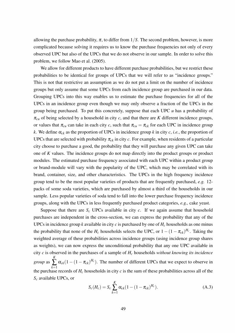
allowing the purchase probability, π , to differ from 1/S. The second problem, however, is morecomplicated because solving it requires us to know the purchase frequencies not only of everyobserved UPC but also of the UPCs that we do not observe in our sample. In order to solve thisproblem, we follow Mao et al. (2005).

We allow for different products to have different purchase probabilities, but we restrict theseprobabilities to be identical for groups of UPCs that we will refer to as “incidence groups.”This is not that restrictive an assumption as we do not put a limit on the number of incidencegroups but only assume that some UPCs from each incidence group are purchased in our data.Grouping UPCs into this way enables us to estimate the purchase frequencies for all of theUPCs in an incidence group even though we may only observe a fraction of the UPCs in thegroup being purchased. To put this concretely, suppose that each UPC u has a probability ofπcu of being selected by a household in city c, and that there are K different incidence groups,or values that πcu can take in each city c, such that πcu = πck for each UPC in incidence groupk. We define αck as the proportion of UPCs in incidence group k in city c, i.e., the proportion ofUPCs that are selected with probability πck in city c. For example, when residents of a particularcity choose to purchase a good, the probability that they will purchase any given UPC can takeone of K values. The incidence groups do not map directly into the product groups or productmodules. The estimated purchase frequency associated with each UPC within a product groupor brand-module will vary with the popularity of the UPC, which may be correlated with itsbrand, container, size, and other characteristics. The UPCs in the high frequency incidencegroup tend to be the most popular varieties of products that are frequently purchased, e.g. 12-packs of some soda varieties, which are purchased by almost a third of the households in oursample. Less popular varieties of soda tend to fall into the lower purchase frequency incidencegroups, along with the UPCs in less frequently purchased product categories, e.g., cake yeast.

Suppose that there are Sc UPCs available in city c. If we again assume that householdpurchases are independent in the cross-section, we can express the probability that any of theUPCs in incidence group k available in city c is purchased by one of Hc households as one minusthe probability that none of the Hc households selects the UPC, or 1− (1−πck)

Hc . Taking theweighted average of these probabilities across incidence groups (using incidence group sharesas weights), we can now express the unconditional probability that any one UPC available incity c is observed in the purchases of a sample of Hc households without knowing its incidence

group asK

∑k=1

αck(1− (1−πck)Hc). The number of different UPCs that we expect to observe in

the purchase records of Hc households in city c is the sum of these probabilities across all of theSc available UPCs, or

Sc(Hc) = Sc

K

∑k=1

αck(1− (1−πck)Hc). (A.3)

49

Mao et al. (2004) note that equation (A.3) can be re-written as:

Sc(Hc) = Sc

K

∑k=1

αck(1− exp(CckHc)) where Cck =− ln(1−πck)

Equation (A.3) is therefore referred to as the “generalized negative exponential” (GNE) model.It is straightforward to see that equation (A.2) is a specific case of equation (A.3) in which theselection probability is identical for all UPCs, i.e., K = 1 and π = 1/S. Moreover, if we knewthe share of all goods in each incidence group, αck, and the probability that each UPC waspurchased, πck, (A.3) would just give us the equation of a particular accumulation curve for acity.

Fortunately, we can use maximum likelihood estimation to estimate Sc as well as the αck

and πck for any choice of K. The number of households purchasing product u in city c, hcu,follows a binomial distribution where the probability of observing hcu purchases is given by:

P(hcu) = ϕ(hcu;πcu) =

(Hc

hcu

)(πcu)

hcu(1−πcu)(Hc−hcu) (A.4)

where Hc is the total number of households in the sample for city c,(Hc

Hcu

)≡ Hc!

hcu!(Hc−hcu)!

and once again πcu = πci for each UPC, u, in category k. Let {hcu}u∈Ucbe the observed counts

of each UPC purchased by our sample of households in a city c, where Uc is the set of UPCsobserved in the city c sample. Now, we can define the binomial mixture distribution as follows:

Φ(hcu) =K

∑k=1

αckϕ(hcu;πck)

This distribution tells us the unconditional probability of observing hcu purchases of any UPC u

in our data, regardless of its incidence group, given the size and purchase probabilities of eachof the incidence groups.

Mao et al. (2005) derive a maximum likelihood methodology for estimating the α’s and π’sfor a given K using data on the number of samples (in our case, households) in which eachvariety is observed. The variable nc j is defined to be the number of products that are purchasedby j households in the dataset for city c, i.e., for which hcu equals j. In other words, if 100UPCs are purchased by no households, 50 UPCs are purchased by 1 household, and 25 UPCsare purchased by 2 households, then we would have nc0 = 100; nc1 = 50; and nc2 = 25. The

50

joint likelihood of the total number of products available in the city, Sc, and the parameters ofthe mixture distribution is

L(

Sc,{αck,πck}Kk=1

)=

Sc!Hc

∏j=0

nc j!

Hc

∏j=0

Φ( j)nc j

Note that from equation (A.3), we know that the number of available products, Sc, is a func-

tion of the number of observed products, Sc(Hc) =Hc

∑j=1

nc j, and the parameters of the mixture

distribution, {αck,πck}Kk=1. Therefore, we only need to estimate the parameters of the mixture

distribution to derive an estimate for the number of available products. To do so, we will max-imize a conditional likelihood function. Let ϕ(hcu;πcu) be a zero-truncated binomial density,i.e., the probability that a product is purchased by j households conditional on it being pur-

chased by more than one household, and Φ( j) =K∑

k=1αckϕ ( j;πck) be the mixture distribution

over these densities for K incidence groups. If we denote the total number of UPCs that arepurchased by at least one household in the sample nc+, the conditional likelihood function is

L(

Sc,{αck,πck}Kk=1

)=

nc+!Hc

∏j=1

nc j!

Hc

∏j=1

Φ( j)nc j (A.5)

Equation (A.5) gives us the likelihood function as a function of the number of incidencegroups, K. In order to identify the correct number of these groups, we estimate the parametersof mixture distributions for a range of values for K using the conditional likelihood function.Each distribution implies a different estimate for the total number of UPCs available in a city.We then compute the Akaike Information Criterion (AIC) for each value of K in each city. Wechoose between the distributions by selecting the number of incidence groups for all cities equalto the K that maximizes the sum of the AICs across all cities. The intuition for this procedure isthat each additional incidence group improves the fit but adds parameters, and the AIC providesa way of determining how many groups are likely to exist in the data.34

Once we have our estimates for the α’s and π’s, we can use equation (A.3) to obtain an

34We also assume that the sampling is sufficient so that we observe some UPCs purchased in each incidencegroup. We need this assumption because we cannot say anything about the number of goods in an incidence groupthat are purchased with such low a probability that no one in the sample ever buys them. In other words, we canonly discuss the number of available varieties for observable classes of goods.

51

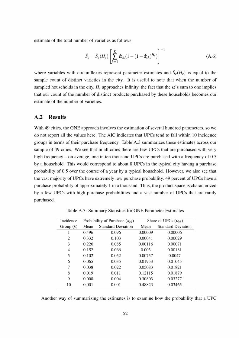
estimate of the total number of varieties as follows:

Sc = Sc(Hc)

[K

∑k=1

αck(1− (1− πck)Hc)

]−1

(A.6)

where variables with circumflexes represent parameter estimates and Sc(Hc) is equal to thesample count of distinct varieties in the city. It is useful to note that when the number ofsampled households in the city, Hc approaches infinity, the fact that the α’s sum to one impliesthat our count of the number of distinct products purchased by these households becomes ourestimate of the number of varieties.

A.2 Results

With 49 cities, the GNE approach involves the estimation of several hundred parameters, so wedo not report all the values here. The AIC indicates that UPCs tend to fall within 10 incidencegroups in terms of their purchase frequency. Table A.3 summarizes these estimates across oursample of 49 cities. We see that in all cities there are few UPCs that are purchased with veryhigh frequency – on average, one in ten thousand UPCs are purchased with a frequency of 0.5by a household. This would correspond to about 8 UPCs in the typical city having a purchaseprobability of 0.5 over the course of a year by a typical household. However, we also see thatthe vast majority of UPCs have extremely low purchase probability. 49 percent of UPCs have apurchase probability of approximately 1 in a thousand. Thus, the product space is characterizedby a few UPCs with high purchase probabilities and a vast number of UPCs that are rarelypurchased.

Table A.3: Summary Statistics for GNE Parameter Estimates

Incidence Probability of Purchase (πck) Share of UPCs (αck)Group (k) Mean Standard Deviation Mean Standard Deviation

1 0.496 0.096 0.00009 0.000062 0.332 0.103 0.00041 0.000293 0.226 0.085 0.00116 0.000714 0.152 0.066 0.003 0.001815 0.102 0.052 0.00757 0.00476 0.065 0.035 0.01953 0.010457 0.038 0.022 0.05083 0.018218 0.019 0.011 0.12115 0.018799 0.008 0.004 0.30803 0.0327710 0.001 0.001 0.48823 0.03465

Another way of summarizing the estimates is to examine how the probability that a UPC

52

is purchased varies with city size. We would expect that the probability that any consumerpurchases any one UPC would go down as the range of available UPCs in the city increases.Fortunately, this is easy to examine given that our GNE structure enables us to estimate theaverage probability that a household in city c purchases a UPC by simply calculating

Πc =K

∑k=1

αc,kπc,k.

In Figure A.1, we see that the estimated average probability of purchase (which uses no popu-lation data in its estimation) decreases sharply with city size. A UPC sold in our smallest city,Des Moines, has three times the probability of being purchased by any individual household as aUPC sold in New York. The fact that households in larger cities are much less likely to buy anyindividual UPC is strongly suggestive of the fact that that the parametric estimate of the UPCsavailable in a city is increasing with city size. We test this directly by using the GNE parameter

Figure A.1: Average Purchase Probability vs. Log City Population

DM

LR

Oma

Syr

Alb

Bir

RicLou

GRJac

MemR−DNas

SLC

ChaColSA

IndOrl

Mil

NHKC

Sac

NOOkC

CinPor

B−R

Pit

TamDenStL

SD

Cle

MinPhoSeaMiaAtlHouDalDet

BosPhi

SFDC

Chi LA

NY

0.0

05.0

1.0

15A

vera

ge P

urch

ase

Prob

abili

ty

13 14 15 16 17Ln(Population)

Average Purchase Probability Fitted values

Notes:

1. Average purchase probability is the average of the estimated probability of a household purchasing a UPC in each incidence group

weighted by the estimated share of UPCs in the same incidence group, i.e., Average Purchase Probability in City c = Πc = ∑10k=1 αc,kπc,k .

2. Acronyms on plots reference the city represented, as listed in Table A.1.

estimates to calculate an estimate for total number of varieties in each city and considering howthis varies with city size. Figure A.2a plots how the log estimated number of varieties in eachcity varies with city size. Visual inspection reveals that the relative relationship between theestimated number of varieties and city size using the Weibull and plotted in Figure A.2b is al-most identical to that obtained with the GNE. We can see this even more clearly in Figure A.2cwhere we plot the Weibull asymptotes against the GNE asymptotes. The correlation between

53

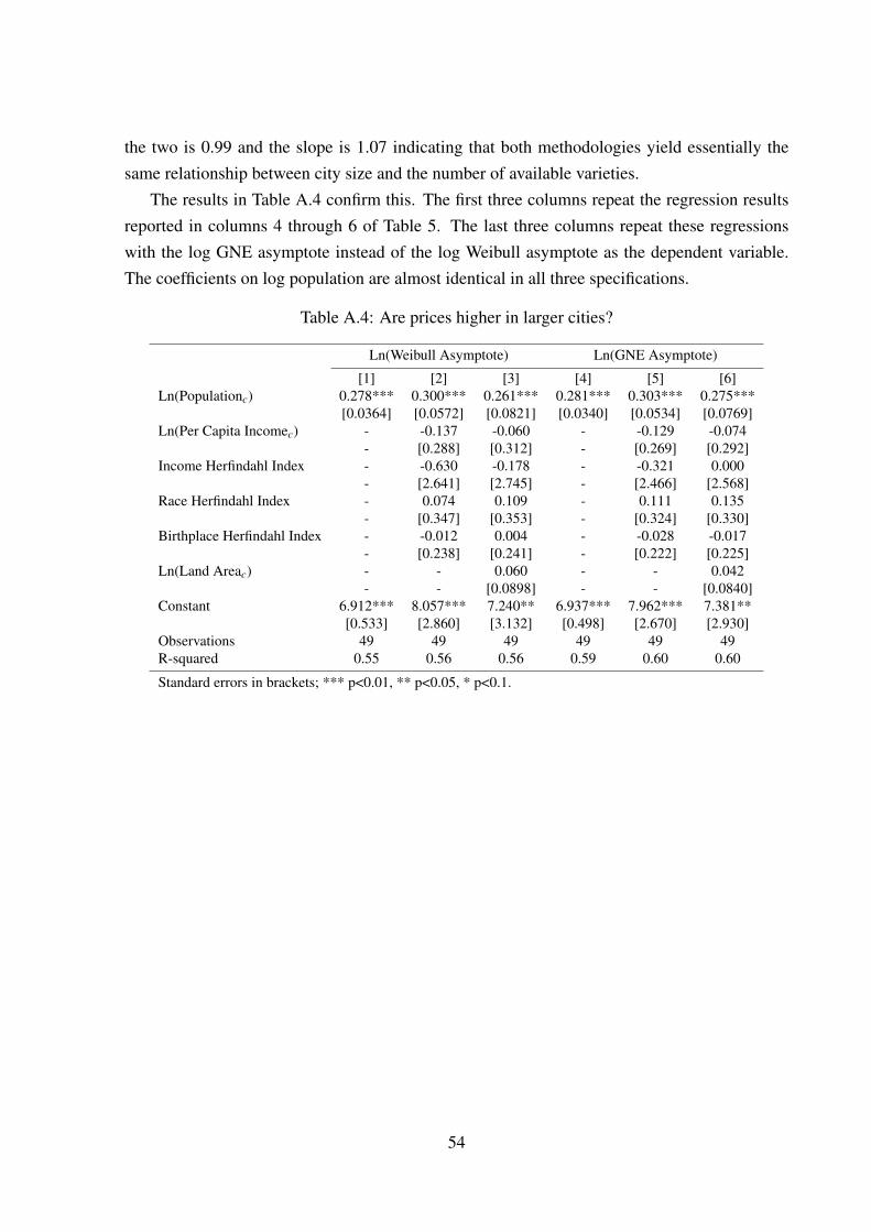
the two is 0.99 and the slope is 1.07 indicating that both methodologies yield essentially thesame relationship between city size and the number of available varieties.

The results in Table A.4 confirm this. The first three columns repeat the regression resultsreported in columns 4 through 6 of Table 5. The last three columns repeat these regressionswith the log GNE asymptote instead of the log Weibull asymptote as the dependent variable.The coefficients on log population are almost identical in all three specifications.

Table A.4: Are prices higher in larger cities?

Ln(Weibull Asymptote) Ln(GNE Asymptote)

[1] [2] [3] [4] [5] [6]Ln(Populationc) 0.278*** 0.300*** 0.261*** 0.281*** 0.303*** 0.275***

[0.0364] [0.0572] [0.0821] [0.0340] [0.0534] [0.0769]Ln(Per Capita Incomec) - -0.137 -0.060 - -0.129 -0.074

- [0.288] [0.312] - [0.269] [0.292]Income Herfindahl Index - -0.630 -0.178 - -0.321 0.000

- [2.641] [2.745] - [2.466] [2.568]Race Herfindahl Index - 0.074 0.109 - 0.111 0.135

- [0.347] [0.353] - [0.324] [0.330]Birthplace Herfindahl Index - -0.012 0.004 - -0.028 -0.017

- [0.238] [0.241] - [0.222] [0.225]Ln(Land Areac) - - 0.060 - - 0.042

- - [0.0898] - - [0.0840]Constant 6.912*** 8.057*** 7.240** 6.937*** 7.962*** 7.381**

[0.533] [2.860] [3.132] [0.498] [2.670] [2.930]Observations 49 49 49 49 49 49R-squared 0.55 0.56 0.56 0.59 0.60 0.60

Standard errors in brackets; *** p<0.01, ** p<0.05, * p<0.1.

54

Figure A.2: Comparing the Weibull and GNE Variety Estimates

(a) Log GNE Estimate vs. Log City Population

DM

LR

Oma

Syr Alb

Bir

Ric

Lou

GRJac

MemR−D

Nas

SLC

ChaCol

SA

IndOrl

Mil

NHKC

Sac

NOOkCCin

Por

B−R

Pit

TamDenStL

SD

Cle

MinPhoSeaMia

AtlHouDal

DetBos

Phi

SF

DC

ChiLA

NY

1010

.511

11.5

Ln(G

NE

Var

iety

Est

imat

e)

13 14 15 16 17Ln(Population)

Ln(GNE Variety Estimate) Fitted values

(b) Log Weibull Variety Estimate vs. Log City Population

DM

LR

Oma

Syr Alb

Bir

Ric

Lou

GRJac

MemR−D

Nas

SLC

ChaCol

SA

IndOrl

MilNHKC

Sac

NOOkCCin

Por

B−R

Pit

Tam

DenStL

SD

Cle

MinPhoSeaMiaAtlHouDal

DetBos

Phi

SF

DC

Chi LA

NY

10.5

1111

.512

Ln(W

eibu

ll A

sym

ptot

e)

13 14 15 16 17Ln(Population)

Ln(Weibull Variety Estimate) Fitted values

(c) Log Weibull Variety Estimate vs. Log GNE Variety Esti-mate

10.5

1111

.5Ln

(Wei

bull

Var

iety

Est

imat

e)

10.4 10.6 10.8 11 11.2 11.4Ln(GNE Variety Estimate)

Ln(Weibull Variety Estimate) Fitted values

Notes:1. Acronyms on plots reference the city represented, as listed in Table A.1.

55

B Formulas for Sato-Vartia Weights

wuc =

suc−sulnsuc−lnsu

∑u′∈Ub

(su′c−su′

lnsu′c−lnsu′

) , wbc =

sbc−sblnsbc−lnsb

∑b′∈Bg

(sb′c−sb′

lnsb′c−lnsb′

) and wgc =

sgc−sglnsgc−lnsg

∑g′∈G

(sg′c−sg′

lnsg′c−lnsg′

)suc, sbc, and sgc are city-specific expenditure shares defined as follows:

suc =vuc

∑u′∈Ub

vu′c, sbc =

∑u∈Ub

vuc

∑b′∈Bg

∑u′∈Ub′

vu′cand sgc =

∑b∈Bg

∑u∈Ub

vuc

∑g′∈G

∑b′∈Bg′

∑u′∈Ub′

vu′c

su, sb, and sg are national expenditure shares defined as follows:

su =vu

∑u′∈Ub

vu′, sb =

∑u∈Ub

vu

∑b′∈Bg

∑u′∈Ub′

vu′and sg =

∑b∈Bg

∑u∈Ub

vu

∑g′∈G

∑b′∈Bg′

∑u′∈Ub′

vu′

for vu = ∑c vuc. G denotes set of product groups, and Gc denotes the set of product groups withproducts sold in city c. Mathematically, Gc = {g ∈ G|Bg 6= /0}. All product groups are sold inevery city, so Gc = G.

56

C How much do Index Formulas Matter?

One concern about comparing the ACCRA fixed-weight methodology with that of the CESexact price index is that there are a host of differences that are difficult to formalize. Twoof these differences seem to be potentially important. First, the ACCRA index uses purposivesampling (i.e. choosing the most commonly purchased variety) while CEPI is constructed usingthe full sample of goods. Second the ACCRA index is a fixed-weight index, but the CEPI adjustsfor substitution bias by using Sato-Vartia weights.

In Table A.5, we show that neither of these differences are quantitatively important forunderstanding our results. The first column of Table A.5 replicates the ACCRA methodologyusing the Nielsen data, as we did in the first column of Table 1, but now using the full set of 49cities instead of the 47 cities for which the ACCRA data was available. Not surprisingly, thecoefficient in the first column of of Table A.5 almost exactly matches that in the first columnof the earlier table. The second column of Table A.5 maintains the same sample of productsused in Column 1 but now recomputes each city’s price index weighting relative category unitvalues with Sato-Vartia weights, rather than ACCRA’s fixed weights; essentially using the CEPIformula to compare category prices, rather than identical UPC prices. The fact that the elasticityof prices with respect to population hardly changes means that simply moving to the correctweighting is not an important factor in understanding why the ACCRA price index overstatesthe relationship between prices and city size.

The importance of product heterogeneity can be easily seen by comparing Columns 2 and3. In Column 3, we continue to use the Sato-Vartia weights for each good category but insteadof comparing the unit value paid for all UPCs in a category (e.g., half gallons of whole milk) wecompare the prices of a single UPC within that category across cities. This procedure eliminatesthe influence played by product heterogeneity in computing the price index, but enables us tocontinue to see the role played by the ACCRA sampling method. The large drop in the elasticityas we move from Column 2 to Column 3 mirrors the large drop that we saw as we moved fromthe first column of Table 1 to the first columns of Table 2 and Table 6, which proves that it isproduct heterogeneity that accounts for the big drop in the association between price and citysize.

Columns 4-6 are drawn from Columns 1, 7, and 9 of Table 6. We include them again forheuristic reasons. In particular, we can see that moving whether we use the ACCRA purposivesample of UPCs (which yields the results in Column 3) or the full sample of UPCs to Col-umn 4 hardly affects the results. However, as we saw earlier, adjusting for the other forms ofheterogeneity bias and the variety bias ultimately flips the sign of the coefficient.

57

Tabl

eA

.5:T

rans

ition

from

the

Rep

licat

ion

ofth

eA

CC

RA

Inde

xto

the

CE

PI

Inde

xM

etho

dolo

gy:

AC

CR

AR

eplic

atio

nU

nadj

uste

dC

EPI

Stor

e-Pu

rcha

serA

djus

ted

CE

PISt

ore-

Purc

hase

rAdj

uste

dE

PI

-Wei

ghts

Fixe

dA

CC

RA

Sato

-Var

tiaSa

to-V

artia

Sato

-Var

tiaSa

to-V

artia

Sato

-Var

tia-U

nitV

alue

Com

pari

sons

With

inC

ateg

ory

With

inC

ateg

ory

With

inU

PCW

ithin

UPC

With

inU

PCW

ithin

UPC

-Sam

ple

Purp

osiv

ePu

rpos

ive

Purp

osiv

eFu

llFu

llFu

llPr

ice

Adj

ustm

ents

Non

eN

one

Non

eN

one

Stor

e&

Purc

hase

rSt

ore

&Pu

rcha

ser

Var

iety

Adj

ustm

ent

Non

eN

one

Non

eN

one

Non

eY

es

[1]

[2]

[3]

[4]

[5]

[6]

Ln(

Popu

latio

n c)

0.04

13**

*0.

0467

***

0.01

31**

*0.

012*

**0.

0041

**-0

.011

***

[0.0

102]

[0.0

147]

[0.0

0368

][0

.003

5][0

.001

8][0

.003

6]C

onst

ant

4.00

0***

-0.6

89**

*-0

.192

***

0.82

***

0.94

***

1.24

***

[0.1

49]

[0.2

15]

[0.0

539]

[0.0

51]

[0.0

27]

[0.0

53]

Obs

erva

tions

4949

4949

4949

R-S

quar

ed0.

260.

180.

210.

210.

100.

17

Stan

dard

erro

rsin

brac

kets

;***

p<0.

01,*

*p<

0.05

,*p<

0.1

58