gome-2 polarisation data and products l.g. tilstra (1,2), i. aben (1), p. stammes (2) (1) sron; (2)...
TRANSCRIPT
GOME-2 polarisation data and products
L.G. Tilstra (1,2), I. Aben (1), P. Stammes (2)
(1)SRON; (2)KNMI
GSAG #42, EUMETSAT, 14-10-2008
2
Validation of GOME-2 polarisation data
Available techniques:
1) focus on special geometries along the orbit where Q/I = 0
2) limiting atmospheres approach
3) focus on the solar irradiance (sunlight is unpolarised)
3
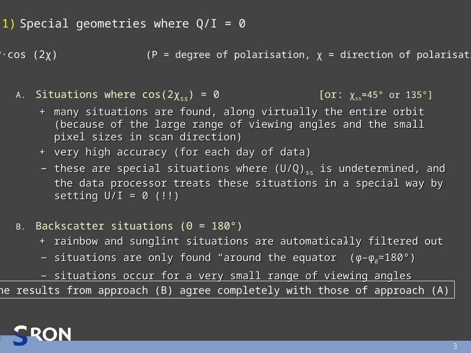
1) Special geometries where Q/I = 0
A. Situations where cos(2χss) = 0 [or: χss=45° or 135°]
++ many situations are found, along virtually the entire orbit (because of the many situations are found, along virtually the entire orbit (because of the large range of viewing angles and the small pixel sizes in scan direction)large range of viewing angles and the small pixel sizes in scan direction)
++ very high accuracy (for each day of data)very high accuracy (for each day of data)
–– these are special situations where (U/Q)these are special situations where (U/Q)ssss is undetermined, and the data is undetermined, and the data
processor treats these situations in a special way by setting U/I = 0 (!!)processor treats these situations in a special way by setting U/I = 0 (!!)
B. Backscatter situations (Θ = 180°)
++ rainbow and sunglint situations are automatically filtered outrainbow and sunglint situations are automatically filtered out
–– situations are only found “around the equator” (situations are only found “around the equator” (φφ––φφ00≈180°)≈180°)
–– situations occur for a very small range of viewing anglessituations occur for a very small range of viewing angles
The results from approach (B) agree completely with those of approach (A)
Q/I = P·cos (2χ) (P = degree of polarisation, χ = direction of polarisation)
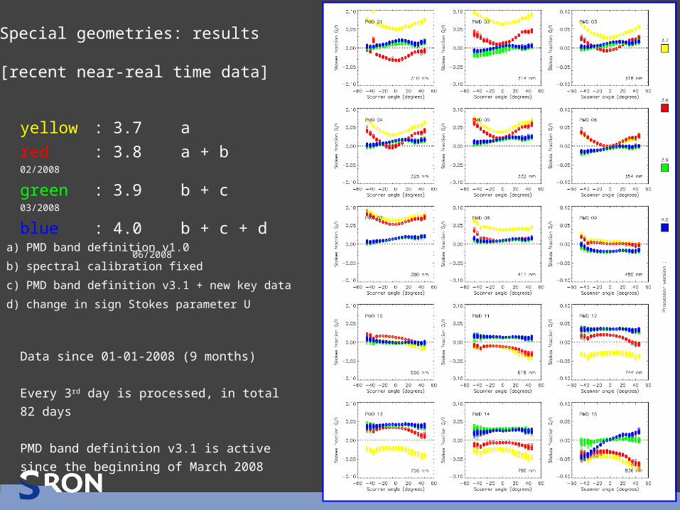
yellow : 3.7 a
red : 3.8 a + b 02/2008
green : 3.9 b + c 03/2008
blue : 4.0 b + c + d 06/2008
Data since 01-01-2008 (9 months)
Every 3rd day is processed, in total 82 days
PMD band definition v3.1 is active since the
beginning of March 2008
a) PMD band definition v1.0
b) spectral calibration fixed
c) PMD band definition v3.1 + new key data
d) change in sign Stokes parameter U
Special geometries: results
[recent near-real time data]
Special geometries: results
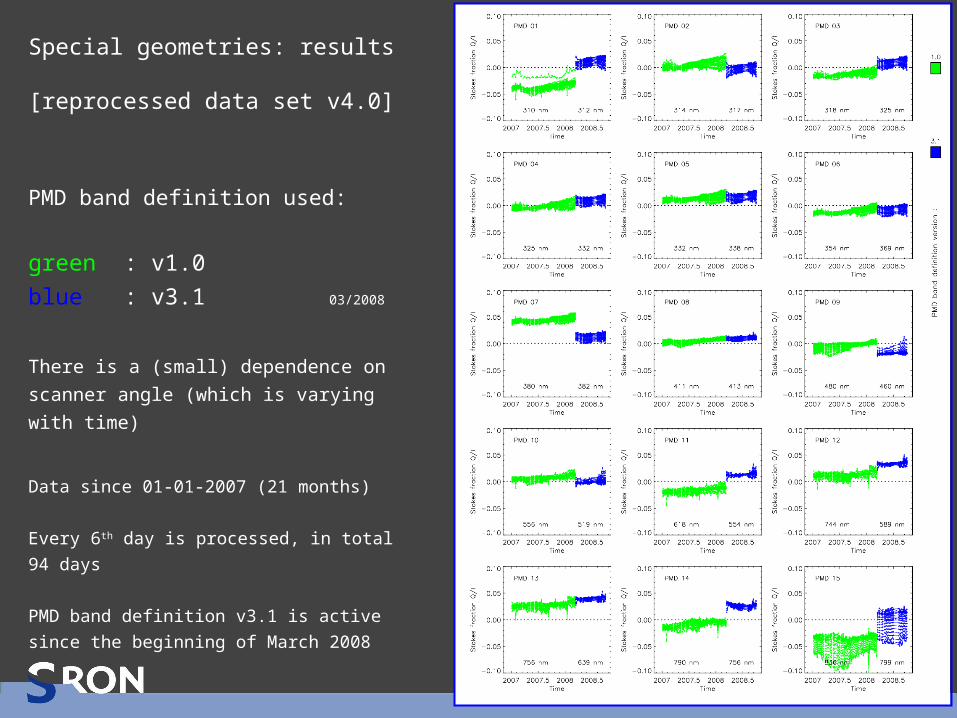
[reprocessed data set v4.0]
PMD band definition used:
green : v1.0
blue : v3.1 03/2008
There is a (small) dependence on scanner
angle (which is varying with time)
Data since 01-01-2007 (21 months)
Every 6th day is processed, in total 94 days
PMD band definition v3.1 is active since the
beginning of March 2008
6
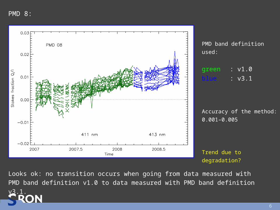
PMD 8:
Looks ok: no transition occurs when going from data measured with PMD band definition v1.0 to data measured with PMD band definition v3.1.
PMD band definition used:
green : v1.0
blue : v3.1
Accuracy of the method:
0.001–0.005
Trend due to degradation?
7
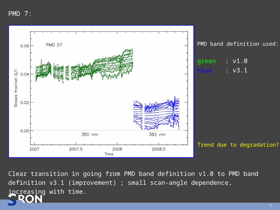
PMD 7:
Clear transition in going from PMD band definition v1.0 to PMD band definition v3.1 (improvement) ; small scan-angle dependence, increasing with time.
PMD band definition used:
green : v1.0
blue : v3.1
Trend due to degradation?
8
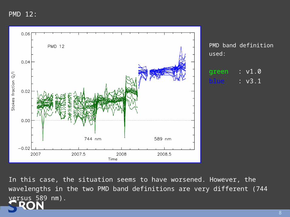
PMD 12:
In this case, the situation seems to have worsened. However, the wavelengths in the two PMD band definitions are very different (744 versus 589 nm).
PMD band definition used:
green : v1.0
blue : v3.1
9
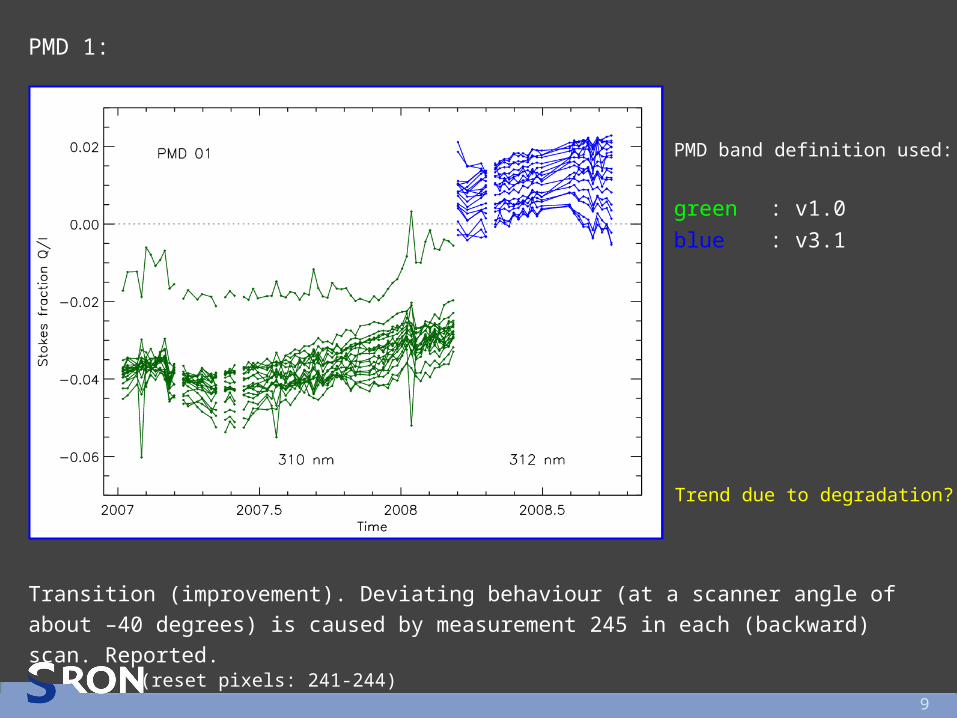
PMD 1:
Transition (improvement). Deviating behaviour (at a scanner angle of about –40 degrees) is caused by measurement 245 in each (backward) scan. Reported.
PMD band definition used:
green : v1.0
blue : v3.1
Trend due to degradation?
(reset pixels: 241-244)
10
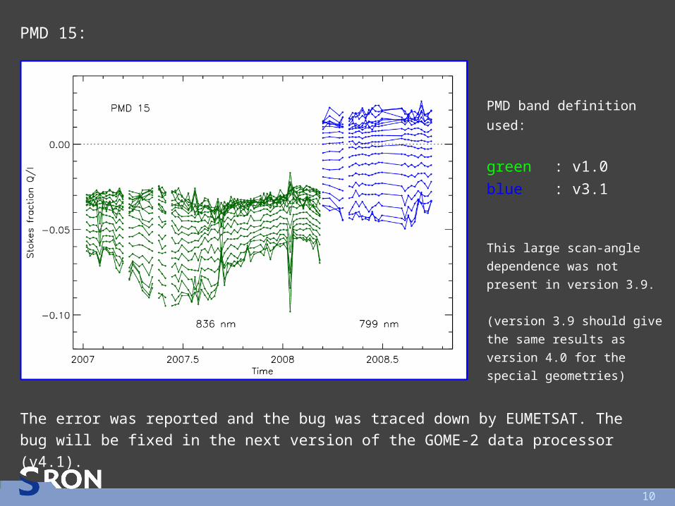
PMD 15:
The error was reported and the bug was traced down by EUMETSAT. The bug will be fixed in the next version of the GOME-2 data processor (v4.1).
PMD band definition used:
green : v1.0
blue : v3.1
This large scan-angle
dependence was not present
in version 3.9.
(version 3.9 should give the
same results as version 4.0
for the special geometries)
11
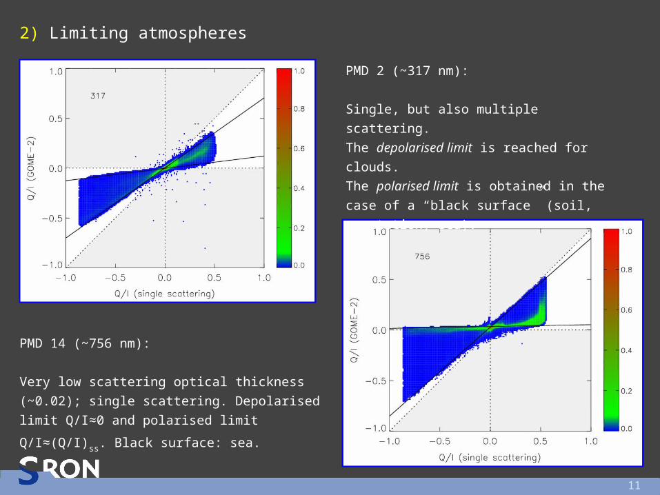
2) Limiting atmospheres
PMD 2 (~317 nm):
Single, but also multiple scattering.
The depolarised limit is reached for clouds.
The polarised limit is obtained in the case
of a “black surface” (soil, vegetation, sea).
PMD 14 (~756 nm):
Very low scattering optical thickness (~0.02);
single scattering. Depolarised limit Q/I≈0 and
polarised limit Q/I≈(Q/I)ss. Black surface: sea.
12
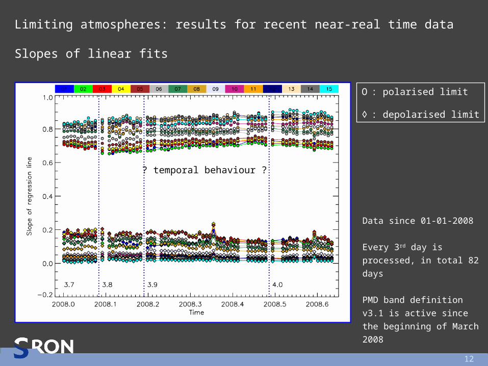
Limiting atmospheres: results for recent near-real time data
Slopes of linear fits
O : polarised limit
◊ : depolarised limit
Data since 01-01-2008
Every 3rd day is processed,
in total 82 days
PMD band definition v3.1 is
active since the beginning
of March 2008
? temporal behaviour ?
13
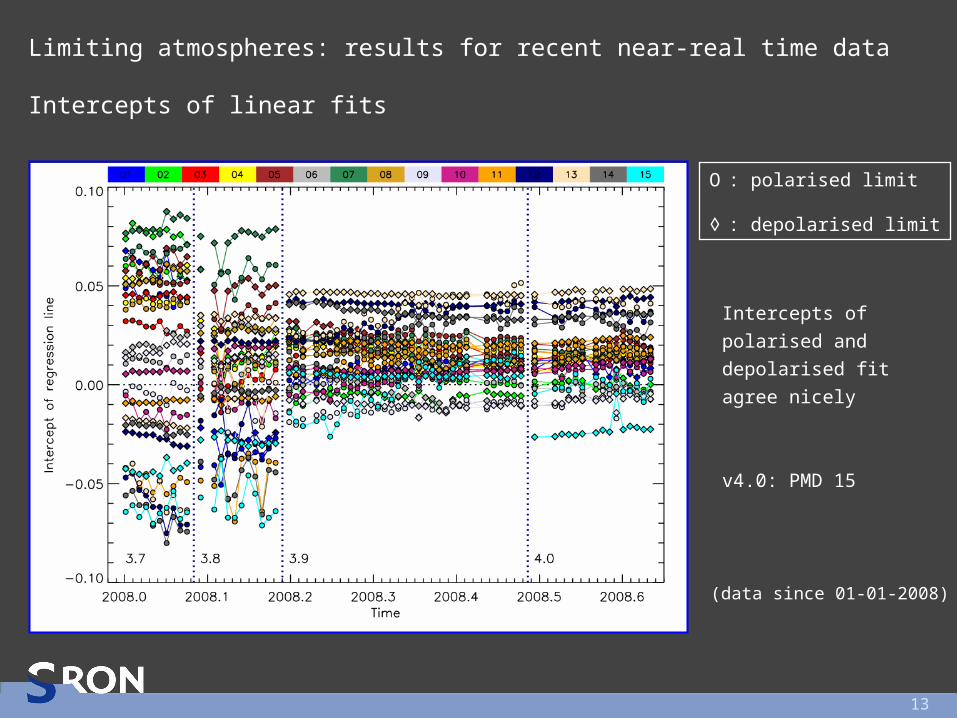
Limiting atmospheres: results for recent near-real time data
Intercepts of linear fits
Intercepts of
polarised and
depolarised fit
agree nicely
v4.0: PMD 15
(data since 01-01-2008)
O : polarised limit
◊ : depolarised limit
14
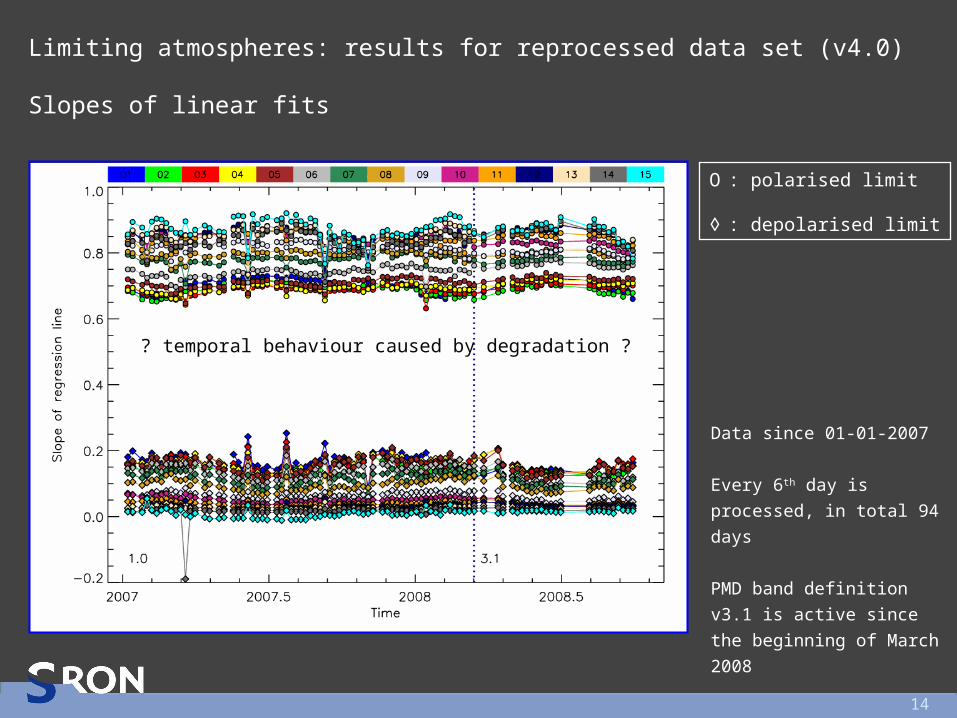
Limiting atmospheres: results for reprocessed data set (v4.0)
Slopes of linear fits
O : polarised limit
◊ : depolarised limit
Data since 01-01-2007
Every 6th day is processed,
in total 94 days
PMD band definition v3.1 is
active since the beginning
of March 2008
? periodic behaviour ?? temporal behaviour caused by degradation ?
15
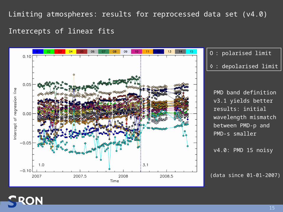
Limiting atmospheres: results for reprocessed data set (v4.0)
Intercepts of linear fits
PMD band definition
v3.1 yields better
results: initial
wavelength mismatch
between PMD-p and
PMD-s smaller
v4.0: PMD 15 noisy
(data since 01-01-2007)
O : polarised limit
◊ : depolarised limit
16
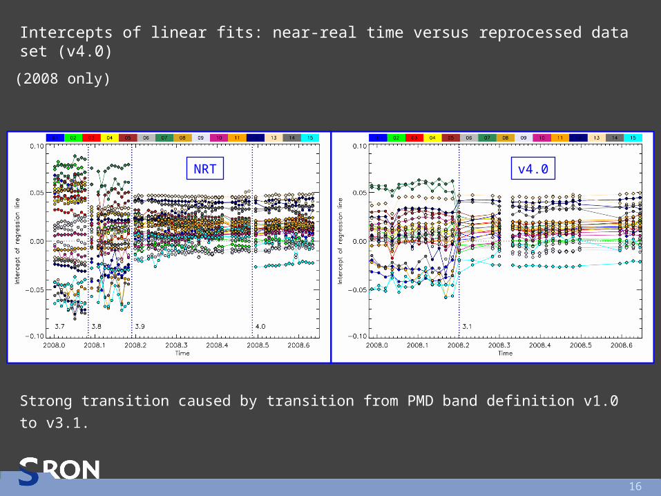
Intercepts of linear fits: near-real time versus reprocessed data set (v4.0)
(2008 only)
v4.0NRT
Strong transition caused by transition from PMD band definition v1.0 to v3.1.
17
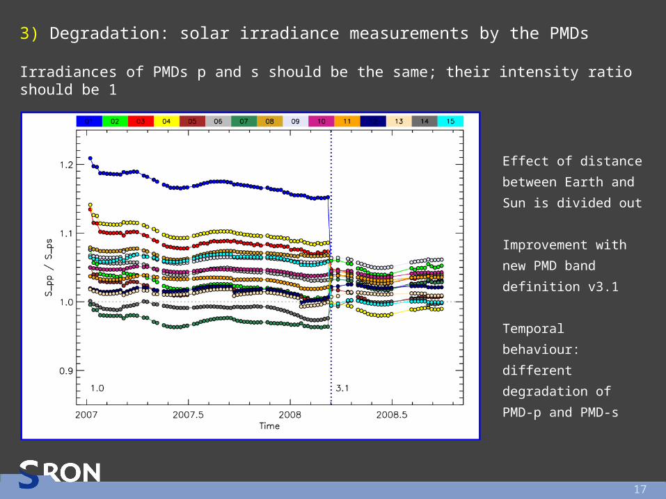
3) Degradation: solar irradiance measurements by the PMDs
Irradiances of PMDs p and s should be the same; their intensity ratio should be 1
(arbitrary normalisation)
Effect of distance
between Earth and
Sun is divided out
Improvement with
new PMD band
definition v3.1
Temporal behaviour:
different degradation
of PMD-p and PMD-s
18
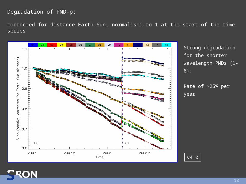
Degradation of PMD-p:
corrected for distance Earth-Sun, normalised to 1 at the start of the time series
Strong degradation for
the shorter wavelength
PMDs (1-8):
Rate of ~25% per year
v4.0
19
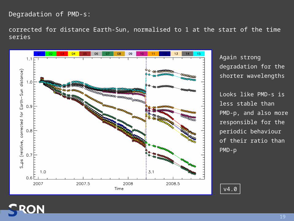
Degradation of PMD-s:
corrected for distance Earth-Sun, normalised to 1 at the start of the time series
Again strong
degradation for the
shorter wavelengths
Looks like PMD-s is
less stable than PMD-p,
and also more
responsible for the
periodic behaviour of
their ratio than PMD-p
v4.0
20
Summary
Special geometry and limiting atmospheres analyses show a very clear
improvement with every data processor version.
In particular, there was a large improvement with the introduction of PMD band
definition v3.1 and new (polarisation) key data.
The scan-angle dependence has been reduced, but is still there to some degree
improve (polarisation) key data even further.
Special geometry and limiting atmospheres analyses have fairly consistent
results, and point to the influence of instrument degradation.
Behaviour of PMD 15 since processor version 4.0: bug fixed in v4.1.
(Relative) degradation correction for the PMDs may be necessary in the future.
This degradation correction is probably scanner-angle dependent.

21
22
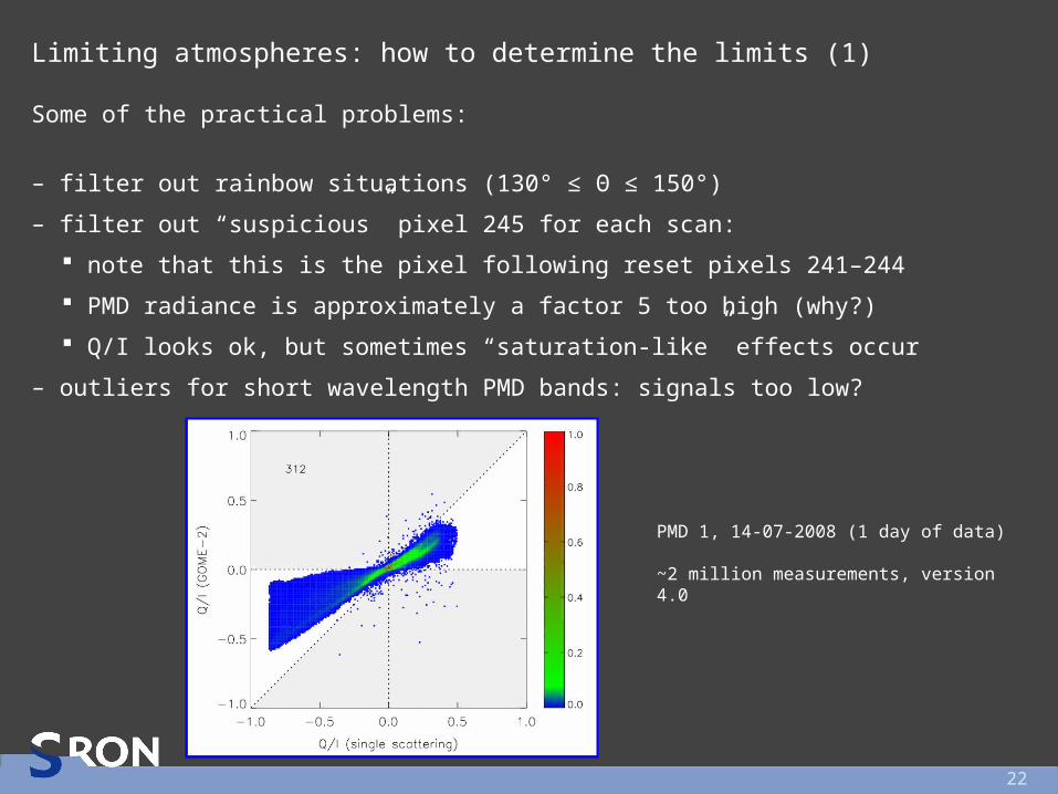
Limiting atmospheres: how to determine the limits (1)
Some of the practical problems:
– filter out rainbow situations (130° ≤ Θ ≤ 150°)
– filter out “suspicious” pixel 245 for each scan:
note that this is the pixel following reset pixels 241–244
PMD radiance is approximately a factor 5 too high (why?)
Q/I looks ok, but sometimes “saturation-like” effects occur
– outliers for short wavelength PMD bands: signals too low?
PMD 1, 14-07-2008 (1 day of data)
~2 million measurements, version 4.0
23
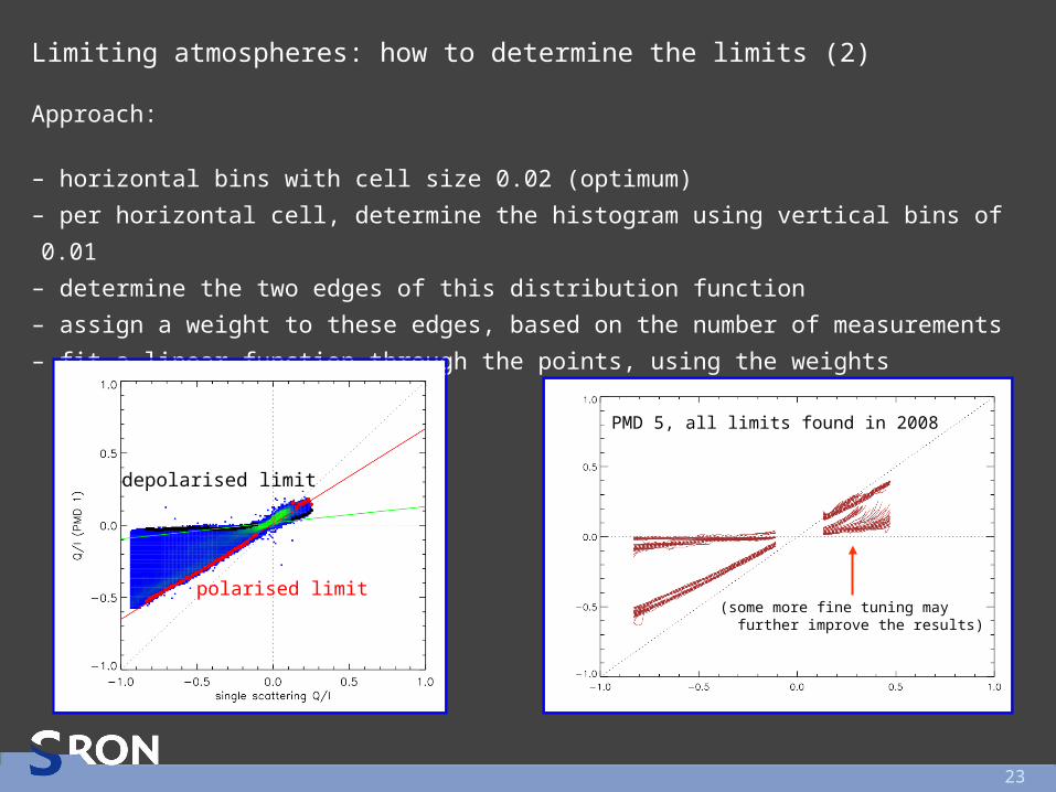
Limiting atmospheres: how to determine the limits (2)
Approach:
– horizontal bins with cell size 0.02 (optimum)
– per horizontal cell, determine the histogram using vertical bins of 0.01
– determine the two edges of this distribution function
– assign a weight to these edges, based on the number of measurements
– fit a linear function through the points, using the weights
depolarised limit
polarised limit
PMD 5, all limits found in 2008
(some more fine tuning may further improve the results)