goce ggm analysis through wavelet decomposition … · reconstruction and validation with...

South-Eastern European Journal

of Earth Observation and Geomatics

Issue Vo4, 2015

13

®Aristotle University of Thessaloniki, Greece Published online March 2015

GOCE GGM analysis through wavelet decomposition and reconstruction and validation with GPS/Leveling data

and gravity anomalies

Athina Peidoua, George Vergosb,* a Dipl. Eng., M.Sc. candidate, Department of Geological Sciences and Geological Engineering,

Queens University, Canada b Assist. Prof., Department of Geodesy and Surveying,

Aristotle University of Thessaloniki

* Corresponding author: [email protected], +302310994366 Abstract: Over the last decade, wavelets (WL) have been exploited widely in many fields of geosciences while they have provided significant outcomes in analyzing gravity field related data in the frequency domain. In this work, we focus on the spectral analysis of GOCE, GOCE/GRACE and combined Global Geopotential Models (GGMs) through wavelet decomposition, filtering and reconstruction in order to improve their performance as to their spectral content in the higher bandwidths of the spectrum. The GGMs evaluated refer to the latest DIR-R4, TIM-R4 and GOCO03S models, which are compared with local GPS/Leveling geoid heights and gravity anomalies, while EGM2008 is used as a reference.

Within a wavelet multi-resolution analysis, both gravity anomalies and geoid heights are analyzed to derive their approximation and detail coefficients for various levels of decomposition, which correspond to different spatial scales. The spectral content at each level is analyzed in order to conclude on the gravity field signal power that GOCE/GRACE GGMs represent compared to EGM2008, especially in the targeted waveband up to 110-150 km. Moreover, various types of low-pass and thresholding denoising filters are investigated to remove high-frequency information from the low resolution GOCE models and adjust the WL reconstruction, respectively. The model synthesis that follows, through coefficient reconstruction, aims at the generation of new synthesized GGMs, where both GOCE, GRACE and EGM2008 information is used, in order to investigate possible improvements in the representation of the Earth’s gravity field. Validation of the synthesized combined GGMs

with available GPS/Leveling geoid heights and terrestrial gravity anomalies is performed, to further assess the improvement brought by the WL analysis. Keywords: Wavelets, gravity field, multi-resolution analysis, selective filtering, thresholding 1. Introduction The gravity field dedicated missions GRACE and GOCE have contributed to the representation of the Earth’s gravity field with increasing accuracy to higher bandwidths of the spectrum. These missions have also provided valuable and reliable data on the time variation and evolution of the gravity field, the latter being a result of mass/water

redistribution in system Earth as well as a response to geodynamic phenomena e.g., mega-earthquakes like the co-seismic gravity change of the Japan Tohoku-Oki earthquake that left a statistically significant signal in the GOCE measured gravity gradients. (Fuchs et al., 2013). Recent results from the evaluation of GOCE/GRACE based GGMs with terrestrial gravity data



Issue Vo4, 2015

14


and deflections of the vertical (Hirt et al., 2011; Tocho et al., 2014; Vergos et al., 2014a) show that GOCE offers improved results between d/o 160 and 185, since for larger degrees of expansion signal loss is experienced. Moreover as far as the geoid concerns, the use of processed GOCE data increases the accuracy of local geoid estimation with gravity data on both ground and sea areas (Barzaghi et al., 2009). Sea level anomaly (SLA) and dynamic ocean topography (DOT) estimation are also influenced from the GOCE advent since both time varying and stationary DOT display errors smaller than 2mm. (Vergos et al., 2014b). The twin GRACE satellites operating in SST-ll (low-low satellite to satellite tracking) model, managed to provide invaluable observations of the spatiotemporal variations of the Earth's gravity field. GRACE observations provide also valuable information concerning the

terrestrial Water storage (Schmidt et al., 2006). This work focuses mainly on the evaluation of GOCE/GRACE-based GGMs, both satellite only and combined ones. Their accuracy assessment is two-fold, since it is based on both the evaluation of gravity anomalies as well as geoid heights. Gravity anomaly evaluation is carried out through local gravity measurements covering the entire European continent, while geoid heights over an extensive network of collocated GPS/Leveling benchmarks, covering continental Greece, are used to assess the accuracy on geoid determination. For this process, wavelet (WL) multi-resolution analysis (MRA) was used. WL MRA was introduced at late 80s’ and is used widely to geosciences over the last twenty years. Although wavelets analysis is too young compared to Fourier analysis that is used for more

than one century, wavelets were developed in order to overcome Fourier localization limitations (Mallat, 1989). In this work WL transform is used to analyze both gravity anomalies and geoid heights in approximation and detail coefficients for various levels of decomposition, which correspond to different spatial scales. To improve the performance of GOCE/GRACE GGMs, as to their spectral content in the higher bandwidths of the spectrums, they are combined through wavelet decomposition, filtering and reconstruction with EGM2008. The aim of this work is to generate new GGMs, where both GOCE, GRACE and EGM2008 are used, and to evaluate these models in order to conclude on the improvements they bring to

gravity field and geoid modeling.

2. Methodology and data used 2.1. Wavelets and wavelet transform It is known, that wavelets offer unique localization capabilities in both the space and frequency domain. Wavelets overwhelmed the Short-time Fourier Transform limitations by functioning with high spatial resolution for high frequencies and low spatial resolutions for low frequencies, in order to clear that the size of the window along the time axes is changed according to the frequency band instead of using a predefined window size for space or frequency localization (Liu, 2010). The choice of the window size creates limitations, and in geosciences there should be a more flexible approach. As a result, wavelets are considered as more effective in signal processing. Wavelet is defined as the function 𝜓(𝑥) which

satisfies the condition 1. 0 < 𝑐𝜓 ≔ 2𝜋 ∫

|�̂�(𝜔)|

|𝜔|

+∞

−∞

𝑑𝜔 < ∞ (1)



Issue Vo4, 2015

15


Wavelet Transformation (WT) is based on certain type of a mother wavelet ψκ(x) and its scaled and translated versions used as basis function in order to represent other functions. An orthonormal wavelet defined as: Where on a measure space 𝑥, the set of square integrable L2-functions is a 𝐿2 space. The 𝐿2-space forms a Hilbert space (Mallat, 1989), that is a complete orthonormal system. After the choice of the wavelet function or mother wavelet, follows the basis function formation, by

the use of translations k and scaling s. These two parameters do not change the basis function. Setting these translations and scaling by means of dyadic translations and dilations of Ψ, so that s=2-j and k=·2-j the wavelet function becomes: where 𝑗, 𝑘 ∈ ℤ By changing the parameters j and k, the behavior of the wavelet can be altered based on

various frequencies (Liu 2010). The wavelet function or mother wavelet {𝜓𝑗𝑘: 𝑗, 𝑘 ∈ ℤ}

carries valuable high frequency information about the signal, while the scaling

function {𝜑𝑗𝑘: 𝑗, 𝑘 ∈ ℤ}, reveals the functional approximation. In respect to Eq. 3 the scaling

function can be defined as: As far as the two-dimensional WL transform is concerned, the wavelet function depends on two arguments (x,y).The translated and scaled basis functions are defined as :

There are three wavelet functions ψH(x,y), ψV(x,y), ψD(x,y), corresponding to the resolution along the x-y, y-x and x-y axis with the bold letter signaling the direction that the details acts upon (Liu, 2010). Since wavelets are base functions with localization properties in both space (time) and

frequency (scale) domains, there can be a multiresolution analysis (MRA) at various levels of decomposition (Chui, 1992). The two-dimensional wavelet transform gives coefficients that correspond to different spatial resolutions, related to the signal frequencies. (Grebenitcharsk and Moore, 2014) According to the decomposition algorithm of wavelets, each scale analysis (level) of the signal, is analyzed in an approximation coefficient that carries the main

𝜓(𝑥) ∈ 𝐿2 (ℝ), 𝑥 ∈ ℝ (2)

𝜓𝑗𝑘(𝑥) = 2𝑗

2⁄ 𝜓(2𝑗𝑥 − 𝑘), (3)

𝜑𝑗𝑘(𝑥) = 2𝑗

2⁄ 𝜑(2𝑗𝑥 − 𝑘). (4)

𝜓𝑗,𝑚,𝑛𝑖 (𝑥, 𝑦) = 2

𝑗2⁄ 𝜓(2𝑗𝑥 − 𝑚, 2𝑗𝑦 − 𝑛) i = {𝐻, 𝑉, 𝐷}, (5)

𝜑𝑗,𝑚,𝑛(𝑥) = 2𝑗

2⁄ 𝜑(2𝑗𝑥 − 𝑚, 2𝑗𝑦 − 𝑛).

(6)



Issue Vo4, 2015

16


approximation information of the signal, and three detail coefficients (horizontal, vertical and diagonal). A new hybrid GGM that is a combination of two GGMs can be generated with respect to spatial resolution through the process of synthesis. Each specific Level of decomposition respects to a spatial scale. Considering the spatial resolution of GGMs different Levels can be composed creating the hybrid GGM. Synthesis is defined as the algebraic sum of the detail coefficients of each Level used and the approximation coefficient of the last Level (Eq.7)

Where the sum of approximation coefficient 12 (A12) and the detail coefficients 12 (𝐻, 𝑉, 𝐷)12 consist Level 12, the sum of detail coefficients (𝐻, 𝑉, 𝐷)11 consist Level 11 etc. The choice of the GGM that will be used in each level depends on its spatial resolution as already mentioned. The spectral content at each level is analyzed in order to conclude on the gravity field signal power that each GOCE/GRACE GGM represents compared to EGM2008. The choice of the GGM that will be used at each level depends on its resolution and the gravity field content w.r.t. EGM2008.

2.2. Filtering When WL transform is implied, the gravity field’s information is transformed from the space to the frequency domain, taking under consideration the Nyquist frequency.. The hybrid GGM generated by the Synthesis process carries noise especially in the higher frequencies, which correspond to the first levels formed by WL transform and reconstruction . This is due to the inherent properties of the data that have been used for the determination of the GOCE/GRACE satellite only GGMs, i.e., the second order derivatives of the Earth’s disturbing potential for GOCE and range-rate data for GRACE. Given the satellite altitude and the consequent attenuation of the gravity field signal with height, GOCE and GRACE manage to

depict with high accuracy the long and medium wavelengths of the gravity field signal. For

those levels that the noise is either dominant or contaminates the gravity field signal, increasing the SNR (signal/noise) demands a digital or spatial filter implementation. A spatial filter changes the value of each pixel using the intensities of neighboring pixel. In terms of this work, Gaussian filter used to remove noise. Gaussian filter decays to zero overcoming problems that other moving average filters have. Having the minimum possible decay, it is considered very effective as far as a space domain filter is concerned and can be described as:

𝑆𝑦𝑛𝑡ℎ𝑒𝑠𝑖𝑠 = 𝐴12 + (𝐻, 𝑉, 𝐷)12 + (𝐻, 𝑉, 𝐷)11 + ⋯ + (𝐻, 𝑉, 𝐷)1 (7)

𝑔(𝑥, 𝑦) =1

2𝜋𝜎2∙ 𝑒

−𝑥2+𝑦2

2𝜎2 (8)

𝐺(𝑢, 𝑣) = 2𝜋𝜎2𝑒−2𝜋2𝜎2(𝑢2+𝑣2), (9)



Issue Vo4, 2015

17


where, x is the distance from the origin in the horizontal axis, y is the distance from the origin in the vertical axis, σ is the standard deviation of the Gaussian distribution, u and v denote radial wavenumbers. Another, useful filter, frequently used in geosciences, is the boxcar filter. It is a smoothing mathematical function, which uses a rectangular window in the frequency domain. This filter is applied to time or frequency series of equal value that goes to zero at a specified time/frequency on each end of the boxcar window. It can be expressed in terms of distribution as

where, λc denotes the cut-off wavelength, ωc the cut-off frequency and ∏(∙) denotes the rectangular function (our idea low-pass filter) with width 2ωc. In the space domain, image filters operate by performing a mathematical operation on each pixel using the pixels surrounding it to generate the result. The size of the boxcar filter determines how big that neighborhood is.

2.3. Thresholding It is known that the smaller the value of coefficient is the more noise it carries, while coefficient with greater values have better quality, because of the energy compaction during the wavelet transform. To reduce the effect of the coefficients with greater values, Soft Thresholding (ST) is implemented, while a Hard Thresholding (HT) is implemented in order to minimize the small coefficients’ contribution. (Russ, 2011) In HT, a value θ is chosen in order to minimize all the small coefficients, keeping unaffected values bigger than θ 𝜏𝜃: ℝ+ → ℝ , as:

Instead, ST changes the values of big coefficients, as: If a coefficient value is smaller than θ then its’ contribution is eliminated. In order to find the value of θ, Donoho and Johnstone (1993), suggested that Thresholding value can be described as

where, Ν is the number of the grid points and �̂� an a-priori std of the noise.

𝑔(𝑥, 𝑦) = 2𝜆𝑐𝑠𝑖𝑛𝑐(2𝜆𝑐(𝑥2 + 𝑦2)), (10)

𝐺(𝑢, 𝑣) = ∏ (𝜔

2𝜔𝑐) (11)

𝜏𝜃(𝑥) = { 0 𝑖𝑓 0 ≤ 𝑥 ≤ 𝜃

𝑥 𝑖𝑓 𝑥 > 𝜃

(12)

𝜏𝜃(𝑥) = { 0 𝑖𝑓 0 ≤ 𝑥 ≤ 𝜃𝑥 − 𝜃 𝑖𝑓 𝑥 > 𝜃

(13)

𝜃𝑈𝑛𝑖𝑣𝑒𝑟𝑠 = �̂�√2𝑙𝑜𝑔𝑁, (14)



Issue Vo4, 2015

18


The process to apply threshold in wavelets, starts with a two-dimensional wavelet transform. The signal is dilated into levels, each composed from an approximation coefficient and detail coefficients. Then threshold is implemented to the coefficients, followed by an Inverse Discrete Wavelet Transform which reveals the denoised image. Inverse Discrete Wavelet Transform (IDWT) is a process by which components can be assembled back into the original signal without loss of information (Bahlmann 2013). This process is called reconstruction. After every level of decomposition only the approximation of the signal is reconstructed, while the detail information use to be kept unchanged per every level.

2.4. Methodology and data used Figure 1 displays the methodology followed. After inputting gravity anomalies (Δg) and geoid heights (N) we imply discrete wavelet transformation (DWT), where each Level of decomposition corresponds to a spatial scale. Then noisy frequencies at specific levels are filtered and the synthesis process takes place. Finally, the hybrid GGM that is generated from the synthesis process is validating by using external data. The present study is focused in the entire European Continental, within the region bounded between−10𝜊 ≤ 𝜆 ≤ 30𝜊 and 30𝜊 ≤ 𝜑 ≤ 60𝜊.Gravity Anomalies and Geoid Heights derived from GOCE/GRACE GGM’s are investigated, while EGM2008 is used as a reference, for the synthesis process. EGM2008 (Earth Gravitational Model 2008) presents a spherical

harmonics expansion of the Earth’s potential to a maximum degree nmax=2159, consisting of both satellite (GRACE, CHAMP, SLR) and local data (Pavlis et al., 2008; 2012).

Figure 1. WL-based MRA processing strategy.



Issue Vo4, 2015

19


GOCO03S (Goiginger et al., 2010; Mayer-Gurr et al., 2012; Pail et al., 2011) presents a spherical harmonics expansion of the Earth’s potential to a maximum degree nmax=250 employing (a) 7.5-years ITG-GRACE2010s data (d/o 180), (b) 18-months of GOCE Satellite Gravity Gradiometry (SGG) observations, (d/o 250), (c) 12-months of GOCE satellite-to-satellite tracking in high-low mode (SST-hl), (d/o 110), (d) 8-years of CHAMP data, and (d/o 120) and (f) 5-years of SLR data from 5 satellites (d/o 5). TIM_R4 (Pail et al., 2011) presents a spherical harmonics expansion of the Earth’s potential to a maximum degree nmax=250, employing 26.5 months of GOCE data. DIR_R4 (Bruinsma et al., 2010), presents a spherical harmonics expansion of the Earth’s potential to a maximum degree nmax=260. It is based on data from GOCE (27.5 months), GRACE (9 years) and LAGEOS. EIGEN-6C2 is a combined

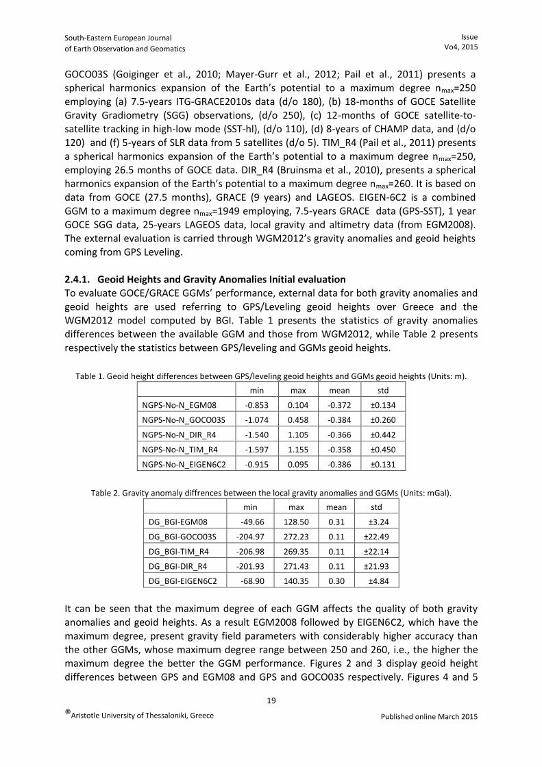
GGM to a maximum degree nmax=1949 employing, 7.5-years GRACE data (GPS-SST), 1 year GOCE SGG data, 25-years LAGEOS data, local gravity and altimetry data (from EGM2008). The external evaluation is carried through WGM2012’s gravity anomalies and geoid heights coming from GPS Leveling. 2.4.1. Geoid Heights and Gravity Anomalies Initial evaluation To evaluate GOCE/GRACE GGMs’ performance, external data for both gravity anomalies and geoid heights are used referring to GPS/Leveling geoid heights over Greece and the WGM2012 model computed by BGI. Table 1 presents the statistics of gravity anomalies differences between the available GGM and those from WGM2012, while Table 2 presents

respectively the statistics between GPS/leveling and GGMs geoid heights.

Table 1. Geoid height differences between GPS/leveling geoid heights and GGMs geoid heights (Units: m).

min max mean std

NGPS-No-N_EGM08 -0.853 0.104 -0.372 ±0.134

NGPS-No-N_GOCO03S -1.074 0.458 -0.384 ±0.260

NGPS-No-N_DIR_R4 -1.540 1.105 -0.366 ±0.442

NGPS-No-N_TIM_R4 -1.597 1.155 -0.358 ±0.450

NGPS-No-N_EIGEN6C2 -0.915 0.095 -0.386 ±0.131

Table 2. Gravity anomaly diffrences between the local gravity anomalies and GGMs (Units: mGal).

min max mean std

DG_BGI-EGM08 -49.66 128.50 0.31 ±3.24

DG_BGI-GOCO03S -204.97 272.23 0.11 ±22.49

DG_BGI-TIM_R4 -206.98 269.35 0.11 ±22.14

DG_BGI-DIR_R4 -201.93 271.43 0.11 ±21.93

DG_BGI-EIGEN6C2 -68.90 140.35 0.30 ±4.84

It can be seen that the maximum degree of each GGM affects the quality of both gravity anomalies and geoid heights. As a result EGM2008 followed by EIGEN6C2, which have the

maximum degree, present gravity field parameters with considerably higher accuracy than the other GGMs, whose maximum degree range between 250 and 260, i.e., the higher the maximum degree the better the GGM performance. Figures 2 and 3 display geoid height differences between GPS and EGM08 and GPS and GOCO03S respectively. Figures 4 and 5



Issue Vo4, 2015

20


display gravity anomalies differences between WGM2012 and EGM08 and WGM2012 and GOCO03S respectively. These figures assess visually the impact that the maximum degree of GGMs has to the accuracy.

Figure 2. GPS and EGM2008 Geoid heights

differences.

Figure 3. GPS and GOCO03S Geoid heights

differences.

Figure 4. WGM2012 and EGM008 Gravity anomalies

differences.

Figure 5. WGM2012 and GOC03S Gravity

anomalies differences.

3. Wavelet MRA of GOCE/GRACE GGMs and accuracy improvement 3.1. GOCE/GRACE GGM MRA in terms of geoid heights As already mentioned, the analysis of the GOCE/GRACE GGMs is performed following a WL-based MRA and assessing their performance in terms of geoid heights and gravity anomalies. Given GOCE and GRACE orbital characteristics and measurement principals, we would

expect to get reliable information up to frequencies corresponding to spatial scales of ~120

km and maybe up to ~90 km. These correspond to degree and order (d/o), of a spherical

harmonics expansion of the Earth’s potential, between 195-225, the latter being the highest d/o that GOCE could probably represent reliably and with a good SNR.



Issue Vo4, 2015

21


In order to analyze signal via wavelets the grid step was used as basis for the number of levels to be defined during the analysis of the input signal, where the step was converted to km. Each Level of decomposition corresponds to a spatial resolution. The first level extends

from 5.5km~11km, the second from 11~22km etc., until the last levels’ spatial analysis

reaches the earth’s perimeter. As a result when the grid step is 3 arcmin, there are 12 Levels of decomposition. In Figure 5 the decomposition levels from the WT of EGM2008 geoid heights are displayed. Each GGM was decomposed into 12 levels, where each level is analyzed in an approximation coefficient and three detail coefficients. After the decomposition of the models follows the reconstruction of levels by combining its detail coefficients, and then the synthesis, as:

Through the synthesis process various GGMs can be combined, since each Level can be composed by a different GGM given each spatial resolution and performance at each specific Level of analysis. Synthesis is defined as the algebraic sum of the detail coefficients of each Level used and the approximation coefficient of the last Level. In order to have a one-to-one

analogy between each level of decomposition and the spatial resolution of the GGMs in terms of harmonic degrees one can apply the simple relationship: Given their maximum degree of spherical harmonics expansion, the resolution that each model has is presented in Table 3. The values presented in Table 3 indicate the smallest spatial scales resolvable by each GGM, i.e., spatial scales beyond those would just contain interpolation errors.

The spectral content at each level is analyzed in order to conclude on the gravity field signal power that each GOCE/GRACE GGM represents compared to EGM2008. The choice of the GGM that will be used at each level depends on its resolution and the gravity field content w.r.t. EGM2008. Given the above analysis, four synthesis scenarios have been considered, where each GOCE/GRACE GGM is synthesized with EGM2008 to improve their spatial resolution and spectral content. Table 4 presents analytically the scenarios investigated and the way the synthesis has been performed. For example, Synthesis 1 means that EGM2008 has been used for the first four levels, then GOCO03S for Level 5, Level 6 and Level 7 and then EGM2008 for Levels 8-12. The rest of the synthesis scenarios follow the same logic. After the synthesis, new combined GOCE/GRACE GGM geoid heights are determined, combining information from GOCE/GRACE for specific levels (i.e., satellite data) and

EGM2008 (i.e., contribution from local data) for the higher resolution Levels were revealed. Table 5 displays differences between GPS/Leveling and the WL MRA synthesis. It can be seen that the standard deviation (std) is improved by as much as 20 cm and the range by more than 50 cm, for the low-

𝑆𝑦𝑛𝑡ℎ𝑒𝑠𝑖𝑠 = 𝐴12 + 𝐻12 + 𝑉12 + 𝐷12 + 𝐻11 + 𝑉11 + 𝐷11 + ⋯ + 𝐻1 + 𝑉1 + 𝐷1 (15)

𝑛 =180°

𝐷𝑒𝑔𝑟𝑒𝑒× 110𝑘𝑚

(16)

Level 12 Level 11 Level 1



Issue Vo4, 2015

22


showing that simple synthesis of the various levels is not enough in order to achieve a performance equal or better than EGM2008.

a. b.

c.

Figure 6. Decomposition analysis of EGM2008 geoid heights in various levels of decomposition. a:

Decomposition analysis of EGM2008 geoid heights in various levels of decomposition. Levels 1-4. b:

Decomposition analysis of EGM2008 geoid heights in various levels of decomposition. Levels 5-8. c:

Decomposition analysis of EGM2008 geoid heights in various levels of decomposition. Levels 9-12.

Table 3. GGM resolution in terms of their maximum degree of expansion.

Resolution (Km)

EGM2008 9.04

DIR_R4 79.2

GOCO03S 79.2

TIM_R4 79.2

EIGEN6C2 10.16



Issue Vo4, 2015

23


Table 4. GGMs’ Synthesis at various Levels.

Resolution

from (km)

Resolution

to (km)

Synthesis

EGM08-

GOCO03S

Synthesis

EGM08-

TIM_R4

Synthesis

EGM08-

DIR_R4

Synthesis

EGM08-

EIGEN6C2

Level1 5.5 11 EGM08 EGM08 EGM08 EGM08

Level2 11 22 EGM08 EGM08 EGM08 EGM08



Level5 88 176 GOCO03S TIM_R4 DIR_R4 EIGEN6c2



Level8 704 1408 EGM08 EGM08 EGM08 EIGEN6c2





Table 5. Geoid height differences between GPS/Leveling and the WL MRA synthesis (Units: m)

min max mean std

NGPS-No-N_EGM08-GOCO03S -1.083 0.453 -0.387 ±0.259

NGPS-No-N_EGM08-TIM_R4 -1.151 0.399 -0.381 ±0.239

NGPS-No-N_EGM08-DIR_R4 -1.048 0.401 -0.392 ±0.223

NGPS-No-N_EGM08-EIGEN6c2 -0.409 0.638 0.129 ±0.155

3.1.1. Filtering the geoid In order to improve the new synthesized models, spatial filters were implemented. Some experiments have been performed in order to investigate which Level combination scheme provides the best results for the combined GOCO03S model. GOCO03S formal resolution,

based on its maximum degree of expansion, is ~79km. Table 6 summarizes the different

levels that have been used during the synthesis process, and the statistics of GGMs and GPS/Leveling differences acquired.

Table 6. Statistics of geoid differences between GPS measurements and different GGMs’ synthesis scenarios

(Units: m)

min max mean std

NGPS-No-N_EGM08_GOCO03S_6_7 -0.855 0.093 -0.378 ±0.124

NGPS-No-N_EGM08_GOCO03S_7_8 -0.862 0.103 -0.371 ±0.136

NGPS-No-N_EGM08_GOCO03S_6_7_8 -0.858 0.093 -0.381 ±0.123

NGPS-No-N_EGM08_GOCO03S_5_6_7 -1.074 0.458 -0.384 ±0.260

NGPS-No-N_EGM08_GOCO03S_4_5_6_7 -1.750 1.000 -0.371 ±0.419

It can be clearly seen that Level 5 shows the most interesting behavior, since it extends from 88 to 176 km, and it can be assumed that if only resolution higher than 120 km was used



Issue Vo4, 2015

24


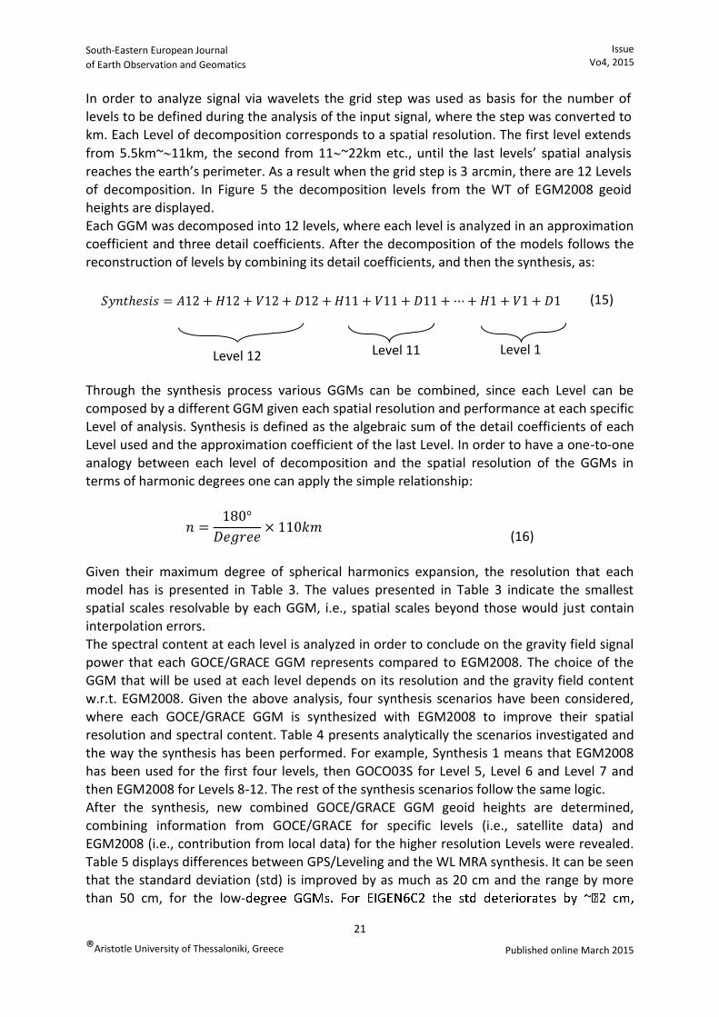
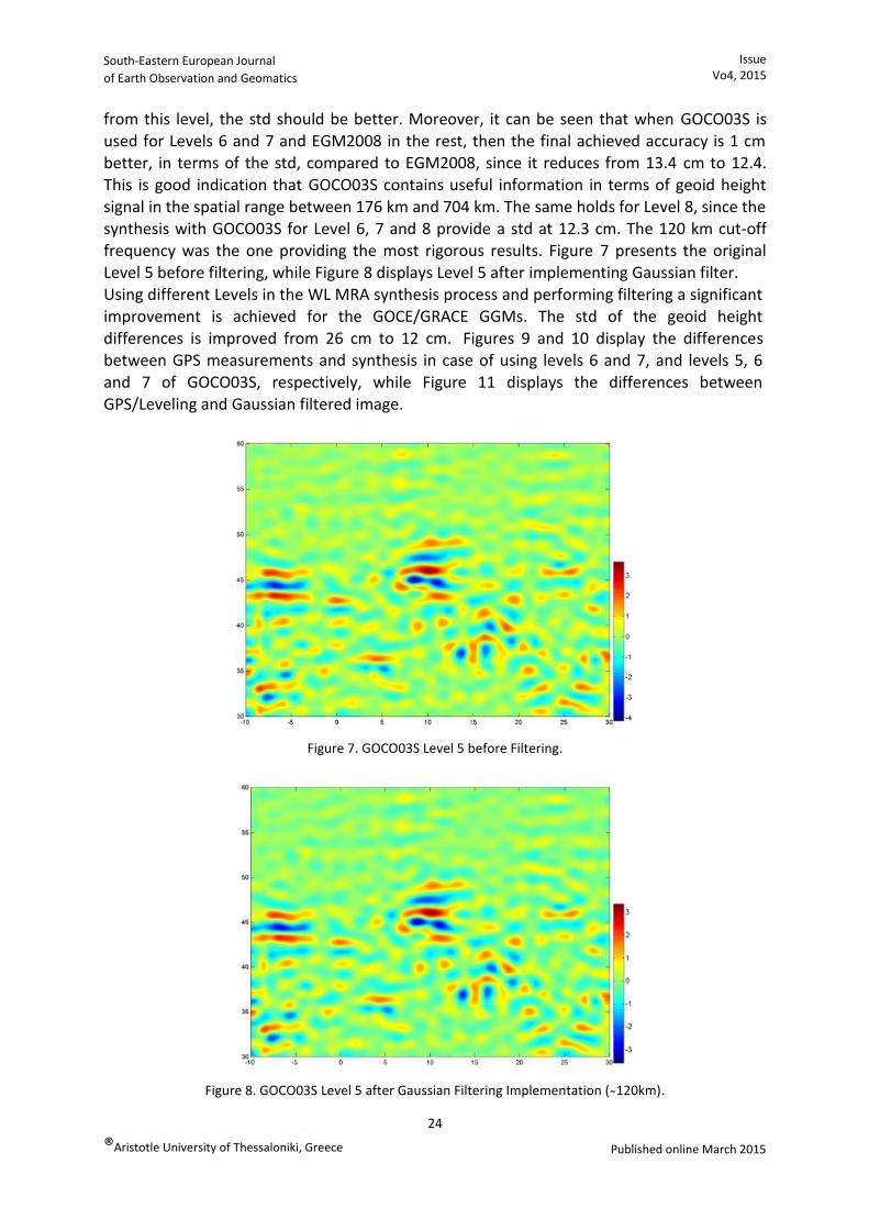
from this level, the std should be better. Moreover, it can be seen that when GOCO03S is used for Levels 6 and 7 and EGM2008 in the rest, then the final achieved accuracy is 1 cm better, in terms of the std, compared to EGM2008, since it reduces from 13.4 cm to 12.4. This is good indication that GOCO03S contains useful information in terms of geoid height signal in the spatial range between 176 km and 704 km. The same holds for Level 8, since the synthesis with GOCO03S for Level 6, 7 and 8 provide a std at 12.3 cm. The 120 km cut-off frequency was the one providing the most rigorous results. Figure 7 presents the original Level 5 before filtering, while Figure 8 displays Level 5 after implementing Gaussian filter. Using different Levels in the WL MRA synthesis process and performing filtering a significant improvement is achieved for the GOCE/GRACE GGMs. The std of the geoid height

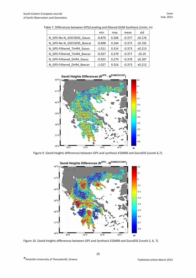
differences is improved from 26 cm to 12 cm. Figures 9 and 10 display the differences between GPS measurements and synthesis in case of using levels 6 and 7, and levels 5, 6 and 7 of GOCO03S, respectively, while Figure 11 displays the differences between GPS/Leveling and Gaussian filtered image.

Figure 7. GOCO03S Level 5 before Filtering.

Figure 8. GOCO03S Level 5 after Gaussian Filtering Implementation ( ̴120km).



Issue Vo4, 2015

25


Table 7. Differences between GPS/Leveling and filtered GGM Synthesis (Units: m)

min max mean std

N_GPS-No-N_GOCO03S_Gauss -0.870 0.206 -0.377 ±0.176

N_GPS-No-N_GOCO03S_Boxcar -0.898 0.244 -0.373 ±0.192

N_GPS-Fiiltered_TimR4_Gauss -1.011 0.314 -0.373 ±0.213

N_GPS-Fiiltered_TimR4_Boxcar -0.927 0.279 -0.377 ±0.19

N_GPS-Fiiltered_DirR4_Gauss -0.925 0.279 -0.378 ±0.187

N_GPS-Fiiltered_DirR4_Boxcar -1.027 0.316 -0.373 ±0.212

Figure 9. Geoid heights differences between GPS and synthesis EGM08 and Goco03S (Levels 6,7).

Figure 10. Geoid heights differences between GPS and Synthesis EGM08 and Goco03S (Levels 5, 6, 7).



Issue Vo4, 2015

26


Figure 11. Geoid heights differences between GPS and gaussian filtered Synthesis.

3.1.2. Thresholding

Another way to eliminate the noise, is to denoise the spatially data through Thresholding. Thresholding, as already mentioned, is incorporated into the DWT and provide reliable results. Implementing the soft Thresholding function, the Thresholding value is setting to t=0.3. Table 8 displays the differences between GPS and thresholded GOCE/GRACE GGMs’ Synthesis. It can be seen that there is slight improvement by 5̴mm at each filtered Synthesis, while GOCO03S is improved by ̴1cm.

Table 8: Differences between GPS measurements and Geoid heights from Thresholded Synthesis (Units: m)

min max mean std

N_GPS-N_GOCO03S_Thresholded -1.074 0.457 -0.385 ±0.251

N_GPS-N_TIM_R4_Thresholded -1.219 0.327 -0.397 ±0.226

N_GPS-N_DIR_R4_Thresholded -1.134 0.375 -0.390 ±0.218

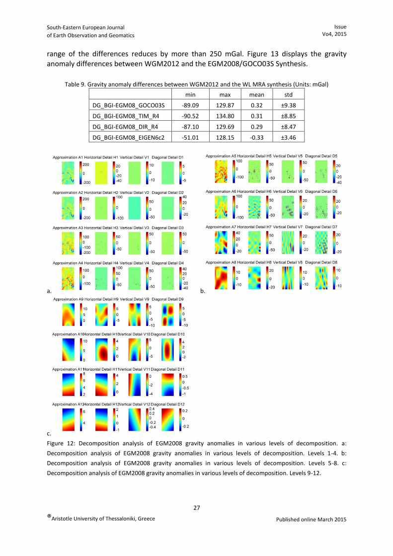
3.2. Gravity anomalies’ Decomposition The same process with geoid heights has been also followed for gravity anomalies. The decomposition of the models was conducted as in the geoid height scenarios discussed previously. In Figure 12 the analyzed decomposition levels of EGM2008 gravity anomalies are displayed. After the DWT and the synthesis process conducted according to Table 4, follows the evaluation of the synthesis. All the synthesized models were compared with Δg from WGM2012. From Table 9, it can be clearly seen that there is a significant improvement

by 8̴.5 mgal when the Synthesis between EGM2008 and GOCE/GRACE GGMs is carried. Table 9 reveals a significant improvement when the WL MRA Synthesis is implemented, since the std of the differences drops by about 13-15mGal. The synthesis of EIGEN6C2 with EGM2008 shows a slight improvement at the 1 mGal level. For the low-degree GGMs the



Issue Vo4, 2015

27


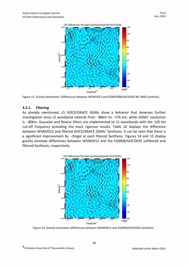
range of the differences reduces by more than 250 mGal. Figure 13 displays the gravity anomaly differences between WGM2012 and the EGM2008/GOCO03S Synthesis.

Table 9. Gravity anomaly differences between WGM2012 and the WL MRA synthesis (Units: mGal)

min max mean std

DG_BGI-EGM08_GOCO03S -89.09 129.87 0.32 ±9.38

DG_BGI-EGM08_TIM_R4 -90.52 134.80 0.31 ±8.85

DG_BGI-EGM08_DIR_R4 -87.10 129.69 0.29 ±8.47

DG_BGI-EGM08_EIGEN6c2 -51.01 128.15 -0.33 ±3.46

a. b.

c.

Figure 12: Decomposition analysis of EGM2008 gravity anomalies in various levels of decomposition. a:

Decomposition analysis of EGM2008 gravity anomalies in various levels of decomposition. Levels 1-4. b:

Decomposition analysis of EGM2008 gravity anomalies in various levels of decomposition. Levels 5-8. c:

Decomposition analysis of EGM2008 gravity anomalies in various levels of decomposition. Levels 9-12.



Issue Vo4, 2015

28


Figure 13. Gravity Anomalies’ Differences between WGM2012 and EGM2008/GOCO03S WL MRA Synthesis.

3.2.1. Filtering As already mentioned, L5 GOCE/GRACE GGMs show a behavior that deserves further investigation since L5 waveband extends from 8̴8km to ̴176 km, while GGMs’ resolution

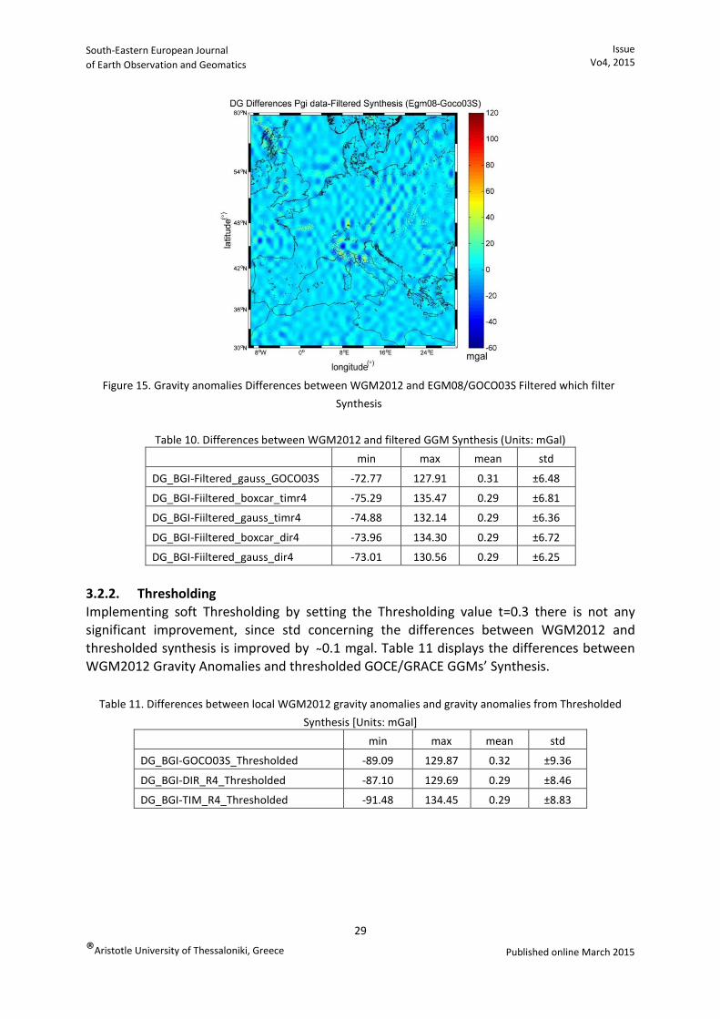
is ̴80km. Gaussian and Boxcar filters are implemented to L5 wavebands with the 120 km cut-off frequency providing the most rigorous results. Table 10 displays the difference between WGM2012 and filtered GOCE/GRACE GGMs’ Synthesis. It can be seen that there is a significant improvement by ̴3mgal at each filtered Synthesis. Figures 14 and 15 display gravity anomaly differences between WGM2012 and the EGM08/GOCO03S unfiltered and filtered Synthesis, respectively.

Figure 14. Gravity anomalies Differences between WGM2012 and EGM08/GOCO03S Synthesis.



Issue Vo4, 2015

29


Figure 15. Gravity anomalies Differences between WGM2012 and EGM08/GOCO03S Filtered which filter

Synthesis

Table 10. Differences between WGM2012 and filtered GGM Synthesis (Units: mGal)

min max mean std

DG_BGI-Filtered_gauss_GOCO03S -72.77 127.91 0.31 ±6.48

DG_BGI-Fiiltered_boxcar_timr4 -75.29 135.47 0.29 ±6.81

DG_BGI-Fiiltered_gauss_timr4 -74.88 132.14 0.29 ±6.36

DG_BGI-Fiiltered_boxcar_dir4 -73.96 134.30 0.29 ±6.72

DG_BGI-Fiiltered_gauss_dir4 -73.01 130.56 0.29 ±6.25

3.2.2. Thresholding Implementing soft Thresholding by setting the Thresholding value t=0.3 there is not any significant improvement, since std concerning the differences between WGM2012 and

thresholded synthesis is improved by ̴0.1 mgal. Table 11 displays the differences between WGM2012 Gravity Anomalies and thresholded GOCE/GRACE GGMs’ Synthesis.

Table 11. Differences between local WGM2012 gravity anomalies and gravity anomalies from Thresholded

Synthesis [Units: mGal]

min max mean std

DG_BGI-GOCO03S_Thresholded -89.09 129.87 0.32 ±9.36

DG_BGI-DIR_R4_Thresholded -87.10 129.69 0.29 ±8.46

DG_BGI-TIM_R4_Thresholded -91.48 134.45 0.29 ±8.83



Issue Vo4, 2015

30


Figure 16. Gravity anomalies differences between WGM2012 and EGM08/GOCO03S thresholded Synthesis.

4. Conclusions A detailed evaluation has been carried out for the recent GOCE and GOCE/GRACE GGMs both in terms of geoid heights and gravity anomalies. From the evaluation that referred to

geoid heights, it was concluded that the generated from MRA synthesis GGMs improve the estimated geoid heights, since compared to local GPS/Leveling data, the std is reduced from ±0.26 m to ±0.13 m, in the GOCO03S case. As far as maximum resolvable wavelengths of GOCO03S, and the rest GOCE/GRACE GGMs, are concerned, it can be concluded that

frequencies higher than ~120 km carry more noise than signal.

As far as the evaluation with gravity anomalies is concerned, the GGMs provide data with higher accuracy (≈20 mgal) than geoid height (≈35 mgal). Through the synthesis process, the std is reduced from ±22 mGal to ±8.8 mGal, for GOCO03S. The classical Gaussian and Boxcar filters, that were implemented to Level 5 (88km~176km), improved the final generated GGM by reducing the std from ±0.25 m to ±0.17 m for geoid heights, while when implementing to

gravity anomalies’ level 5, they reduce the std from ±9.375 mGal to ±6.481 mGal. The thresholding method, improved slightly not only geoid heights, but also gravity anomalies, by 7 mm and 0.01 mGal, respectively. The proposed WL MRA methodology for the analysis and synthesis of GOCE/GRACE GGMs provides overall promising results since the std is improved my more than 55% for both geoid heights and gravity anomalies. Our future work will be directed to selective filtering of individual frequencies, rather than applying a unified filter to an entire Level of decomposition. In that way, specific frequencies that seem problematic (low SNR, blunders, etc.) will be removed without affecting the rest of the frequencies that belong to the same decomposition level. References

Bruinsma S., 2010, GOCE gravity field recovery by means of the direct numerical method. Presented at the ESA Living Planet Symposium, Bergen, Norway.

Chui C., 1992, An Introduction to Wavelets. Academic Press, 1st Ed., ISBN-13, pp. 978-0121745844.



Issue Vo4, 2015

31


Donoho D., Johnstone M, 1998, Minimax estimation via wavelet shrinkage. The Annals of Statistics, Volume 26, Issue 3: 879-921.

Goiginger, H., 2011, The combined satellite-only global gravity field model GOCO02S. presented at the 2011 General Assembly of the European Geosciences Union, Vienna, Austria.

Grebenitcharsky R., Moore P., 2014, Application of Wavelets for Along-Tracking Multi-Resolution Analysis of GOCE SGG Data. In: Marti U (ed) Gravity, Geoid and Height Systems, International Association of Geodesy Symposia Volume 141, Springer International Publishing Switzerland, pp: 41-50.

Hirt C., Gruber T., Featherstone W., 2011, Evaluation of the first GOCE static gravity field

models using terrestrial gravity, vertical deflections and EGM2008 quasigeoid heights. J Geod, Volume 85, Issue 10: 723-740.

Liu C., 2010, A tutorial of the wavelet transform, Department of Electrical Engineering, National Taiwan University.

Mallat S., 1989, A theory for multiresolution signal decomposition: the wavelet representation. IEEE Trans on Pattern Analysis and Machine Inteligence, Volume 11: 674-693.

Mayer-Gurr T., 2012, The new combined satellite only model GOCO03S. Presentation at GGHS 2012 IAG Symposia, Venice, October 2012.

Pail R., 2011, First GOCE gravity field models derived by three different approaches. J Geod

Volume 85, Issue 11: 819-843. Pavlis N., Holmes S., Kenyon S., Factor J., 2008, An Earth Gravitational Model to Degree

2160: EGM2008, General Assembly of the European Geosciences Union, Vienna, Austria, National Geospatial Intelligence Agency.

Pavlis N, Holmes S, Kenyon S, Factor J, 2012, The Development and Evaluation of the Earth Gravitational Model 2008 (EGM2008). J. Geophys Res 117 (B04406).

Russ C., 2011, The Image Processing Handbook, Sixth Edition. Tocho C., Vergos G., Pacino M., 2014, Evaluation of the latest GOCE/GRACE derived Global

Geopotential Models over Argentina with collocated GPS/Leveling observations. In: Marti U (ed) Gravity, Geoid and Height Systems, International Association of Geodesy Symposia Volume 141, Springer International Publishing Switzerland, pp:

75-83. Vergos G., Grigoriadis V., Tziavos I., Kotsakis C., 2014a, Evaluation of GOCE/GRACE Global

Geopotential Models over Greece with collocated GPS/Levelling observations and local gravity data. In: Marti U (ed) Gravity, Geoid and Height Systems, International Association of Geodesy Symposia Volume 141, Springer International Publishing Switzerland, pp: 85-92.

Vergos G., Natsiopoulos D., Tziavos I., Grigoriadis V., Tzanou E., 2014b, DOT and SLA stationary and time-varying analytical covariance functions for LSC-based heterogeneous data combination. Presented at the 2014 EGU General Assembly, Session G1.1, Recent developments in geodetic theory, Vienna, Austria.



Issue Vo4, 2015

32


goce ggm analysis through wavelet decomposition … · reconstruction and validation with...

Documents