GNG-based foot reconstruction for custom footwear manufacturing 1

Abstract 2 Custom shoes manufacturing is one of the major challenges facing the footwear industry today. A shoe for 3

everyone: it is a change in the production model in which each individual's foot is the main focus, replacing 4 traditional size systems based on population means. This paradigm shift represents a major effort for the 5 industry, for which the design and not production becomes the main bottleneck. It is therefore necessary to 6 accelerate the design process by improving the accuracy of current methods. 7

The starting point for making a shoe that fits the client’s foot anatomy is scanning the surface of the foot. 8 Automated foot model reconstruction is accomplished through the use of the self-organising Growing Neural 9 Gas (GNG) network, which is able to topographically map the low dimension of the network to the high 10 dimension of the manifold of the scanner acquisitions without requiring a priori knowledge of the structure of 11 the input space. 12

The GNG obtains a surface representation adapted to the topology of the foot, is accurate, tolerant to noise, 13 and eliminates outliers. It also improves the reconstruction in "dark" areas where the scanner does not obtain 14 information: the heel and toe areas. The method reconstructs the foot surface 4 times more accurately than 15 other well-known methods. The method is generic and easily extensible to other industrial objects that need to 16 be digitized and reconstructed with accuracy and efficiency requirements. 17

Keywords. custom footwear manufacturing, foot reconstruction, Growing Neural Gas, Marching Cubes. 18

1 INTRODUCTION 19

The evolution of industrial technology has led to the application of the latest advances in traditional 20 manufacturing sectors. Specifically, in the footwear industry, the production systems are being adapted to 21 current market demands, allowing the creation of new business models. These new models aim to incorporate 22 quality improvements, flexibility and cost reduction in the value chain of companies. 23

The high-level customization goal for footwear is to manufacture a pair of shoes for a specific customer. 24 This customer-focused manufacturing aims to achieve quality and comfort, and in some cases even an 25 improvement in the health of customer's foot. Although research into custom shoe design is not new (Hoy et 26 al., 1990), it was not until the early years of this century that research works aimed at ensuring a better fit 27 between foot morphology and shoelast [2-5] were presented. 28

Recently, the researchers have been trying to make proposals that are viable in the industry. Thus in [6], a 29 method for analyzing a shape fit for a particular foot was proposed, by checking a small number of foot 30 sections obtained both in plane and from the shoelast. In [7], a geometric model of the shoelast is adapted to a 31 reference foot in order to automate the proposed process of customized manufacturing. Other studies define 32 CAD tools used to create custom shoes for general [8] and specific medical issues, such as for diabetic 33 patients, who suffer from the disease called "diabetic foot" [9]. 34

The basic starting point in the process of customization of shoes at a high level is the digitization of the 35 reference foot. The aim is to obtain the surface that represents the user's foot whose footwear is going to be 36 customized. The geometry of the foot is represented by a set of points in three-dimensional space that 37 represent the underlying surface of the reference object. The acquisition of basic data (unstructured point 38 cloud) that defines the geometry of the foot is performed using laser devices that provide a set of unorganized 39 points defining the surface. These points need to be treated and filtered to obtain a three-dimensional 40 continuous surface from which the characteristic points and necessary measures to carry out the comparison 41 with the shoe-last are calculated. 42

The digitization process consists in obtaining the key points of the underlying surface geometry to be 43 reconstructed. To obtain these points (point cloud) a wide variety of imaging devices with established features 44 and precision tolerances can be used. Precision is a key factor when capturing the information of a foot, as in 45 the process of building footwear the accuracy required in the last surface should be in the range of +-0.1mm. 46 As an example, footwear usually involves the addition of a customised inlay, so the topographical shape of 47 the base of the foot can be an important factor in manufacture of a suitable pair of shoes. Given this scenario, 48 several types of acquisition modes are available. A good way to determine the morphology of a foot and its 49

internal structure is via a CT (Computed Tomography), which provides all the necessary 3D information. 1 However, despite the goodness of this system it is economically unfeasible to incorporate these devices in the 2 possible locations of system implementation in the footwear industry. It is therefore essential that the 3 characterization is performed standing with the tools that are available on the real market that allow 4 purchasing without assuming a disproportionate economic cost relative to the final result to be obtained, or by 5 using computational elements of medium and low cost that are typical in the footwear industry. 6

7 On the other hand, there are generic devices that allow rapid acquisition and low cost digitization. Such is 8

the case of the system presented in [10], which reconstructs the surface of the foot, and is based on the Kinect 9 ® device. This device has an acquisition error greater than 2 mm and research presents reconstruction errors 10 of more than 10 mm, so it cannot be offered as a valid alternative for the industrial footwear manufacturing 11 process. There are some devices designed to capture the surface of the foot, and such devices offer enough 12 acquisition quality to incorporate them in the industrial manufacturing process, but the information they 13 provide is in the form of clouds of unorganized points that need further reconstruction. 14

15 The objective of this research is to obtain, from an unorganized point cloud acquired via an optical laser 16

scanner, an organized structure of points to adapt the topology of the foot. The process should be fast and 17 accurate in order to ensure both the accuracy requirements in the design of footwear as well as its viability in 18 custom manufacturing processes. The presented method is based on using GNG neural networks that adapt to 19 the topological features of the objects and also performs filtering of erroneous data that may be obtained from 20 the digitizer. 21

22 The article is structured in the following sections. The main contributions to the reconstruction process and 23

the problems that arise when we wish to obtain surfaces for foot reconstruction are presented in Section 2. 24 The fundamentals of the method used, which are based on GNG neural networks, are presented in Section 3. 25 Different experiments aiming to test the efficiency and accuracy of the method are presented in Section 4, 26 along with a comparison with other reconstruction methods. Finally, in Section 5 we highlight the main 27 contributions of this work and future research is presented. 28

2 RECONSTRUCTION METHODS-STATE OF THE ART 29

In this section we review well-known methods and techniques used in the reconstruction of three-dimensional 30 surfaces analyzed from the point of view of requirements for the design and manufacture of shoe lasts. 31

2.1 Delaunay’s alpha-shapes 32

Reconstruction by Delaunay in three dimensions consists in the tetrahedrization of the initial pointcloud. 33 The primary advantage of the majority of the methods based on Delaunay is a very accurately adjustment to 34 the surface defined by the original point cloud. However, the problem that arises is that since it is an 35 interpolation of points operation, the presence of noise produces undesirable results (see figure 1). Therefore, 36 the quality of the points obtained in the scanning process determines the feasibility of these methods. When 37 all points of the point cloud are used to obtain the best possible triangulation, provided the rule of Delaunay, 38 the points of the scanned surface, with an error considered higher than allowed, are explicitly represented on 39 the surface geometry reconstructed. 40

41

1 Fig. 1. Reconstruction with Delaunay: a) point cloud, b) noisy section, c) noisy foot 2

3 One of the earliest approaches is based on α-shapes by [11]. The concept of alpha-shape (alpha-form) 4

formalizes the intuitive notion of "form" for a set of points in space. An alpha-shape simply defines a shape 5 representing the initial set of points at which the chosen alpha value is applied. 6

The alpha-shapes are obtained from the Delaunay triangulation. Given a finite set of points S, and an actual 7 parameter alpha, the alpha-shape of S is a polytope (generalization to any dimension of a two dimensional 8 polygon, and a polyhedron) which is neither convex nor necessarily connected. For a large enough number 9 alpha, alpha-shape is identical to the convex-hull of S. If the alpha value decreases progressively, non-convex 10 shapes with cavities are obtained. 11

Their algorithm eliminates all tetrahedra that are delimited by a smaller sphere surrounding α. The surface 12 is then obtained from the outer triangles of the resulting tetrahedra. Another approach is based on the initial 13 labeling tetrahedrization as interior and exterior. The resulting surface is generated from the triangles found 14 inside and outside. This idea first appeared in [12] and was later performed by Powercrust in [13] and the 15 algorithm called Tight COCONE [14]. Both methods have recently been extended to the reconstruction of 16 point clouds with noise in [15] and [16]. 17

In the reconstruction of point clouds it is necessary to solve two different problems: obtaining the 18 neighborhood of a point and the calculation of the corresponding normal direction. The following sections 19 will define how these critical data are obtained to perform the final process of surface reconstruction. 20

The implementation of any of these techniques in the normal orientation is feasible from the point of view 21 of efficiency of the model, since the time required for reconstruction of foot geometry using these techniques 22 exceed the limits set in the context of the problem. Therefore, due to the specific geometry of a human foot, 23 we propose an ad hoc technique that considerably speeds up the process by taking into account the 24 morphology of that foot. 25

Sections with a number of regular noise as shown in figure 2 may be treated to obtain the alpha-form shape 26 that identifies all points of the section. 27

28

29 Fig. 2. Alpha shapes: a) original noisy section and resulting alpha-shape, b) detail of filtered noise, c) corners 30 31

2.2 Voxel Grid 32 33

The Voxel Grid filtering technique is based on sampling the input space using a 3D voxel grid to perform 34 reduction. This technique has been used traditionally in the area of computer graphics to subdivide the input 35 space and reduce the number of points [17-18]. 36

For each voxel, the centroid is chosen as representative of all content points. There are two approaches, 37 namely picking the centroid of the voxel or choosing the centroid of the points that lie within the voxel. 38 Averaging internal voxel points means greater computational cost but gives better results. Thus, a subset of 39 the input space that represents roughly the underlying surface is obtained. Voxel grid has the same problems 40 as other filtering techniques: impossibility of defining the final number of points representing the surface, loss 41

of geometric information to reduce the points inside a voxel with its centroid, sensitivity to noise and lack of 1 adaptation to input space [19]. 2

2.3 Marching Cubes 3

Implicit reconstruction methods (or zero-set methods) reconstruct the surface based on a distance function, 4 which assigns to each point in space signed distance to the surface. The polygonal representation of the object 5 is obtained by extracting f zero-set using a contour algorithm. Thus, the problem of reconstructing a surface 6 from an unorganized point cloud is reduced to obtaining the appropriate function f which has a zero value at 7 the sampling points and the non-zero elsewhere. In [20] the beginning of the use of such methods was 8 established using the algorithm that was called "the Marching Cubes Algorithm". This algorithm has evolved 9 through the incorporation of different variations: in [21] an f discrete function, was used, and in [22] 10 polyharmonic radial basis functions are used, which are adjusted to the initial set of points. Other approaches 11 include the Moving Least Squares adjustment function [23-24], and basic functions with local support [25], 12 based on the Poisson equation [26]. 13

14 The main problem with these methods is the necessity to obtain the normal of the implicit surface at each 15

of the points of the point cloud. In order to compute the normal vector at a surface point, a tangent plane must 16 be obtained from the vicinity of that point. However, due to the fact that normal orientation must be 17 preserved, this problem is not trivial and its computation has a high cost. 18

Implicit reconstruction methods have the problem of loss of definition of the geometry in those areas where 19 there is extreme curvature, such as corners. Likewise, pretreatment of information by applying some kind of 20 filtering technique also affects the definition of the corners, making them softer. As can be seen in Figure 3, 21 after applying a Gaussian filter shows that the corners have softened, and this is a key problem in addressing 22 reconstruction. 23

24

25 Figure 3 – Softened corner 26

27 28 29 There are various studies dealing with the post processing of the reconstruction, for the detection and 30

refining of corners [24,27]. For anthropomorphic volumes such as the foot, the lack of these geometrically 31 problematic areas from this point of view, means that no treatment is necessary 32

Another problem with Marching Cubes is their behavior in the absence of information, that is, when they 33 have not been able to obtain points in certain areas. Because this algorithm does not consider the topology of 34 the object, it has a tendency to close the information areas without making lumps. In Figure 4, the algorithm 35 produces bulging in an area that has not obtained the digitizer points shown. 36

37 38

1 2

Figure 4 – Reconstruction with Marching Cubes: bulging in areas without points 3 4 5 6 7

3 GNG-based 3D reconstruction 8 9

To obtain the 3D model from the sections obtained from the scanner we propose the use of an Automated 10 landmark extraction method based on the use of the self-organising network the Growing Neural Gas (GNG), 11 which is able to topographically map the low dimension of the network to the high dimension of the manifold 12 of the contour without requiring a priori knowledge of the structure of the input space. 13 14

Landmark-based techniques can be classified as manual, semi-automatic and automatic. Because the first 15 two are laborious and subjective, especially when applied to 3D images, various attempts have been made to 16 automate the process of landmark-based image registration and correct correspondences among a set of 17 shapes. 18

In [28], a method is presented for automatically building statistical shape models by re-parameterising each 19 shape from the training set and optimising an information theoretic function to assess the quality of the model. 20 The quality of the model is assessed by adopting a minimum description length (MDL) criterion for the 21 training set. This is a very promising method and the models that are produced are comparable to, and often 22 better than, the manually built models. However, due to a very large number of function evaluations and 23 nonlinear optimisation the method is computationally expensive. 24

In [29], a modified growing neural gas has been used to automatically match important landmark points 25 from two related shapes by adding a third dimension to the data points and by treating the problem of 26 correspondence as a cluster-seeking method by adjusting the centers of points from the two corresponding 27 shapes. 28

It is known, from aspects of visual perception, that information on the shape of a curve is concentrated at 29 dominant points having the highest curvature. For a given set of ordered points (ordered by time or length), 30 dominant points detection through curvature estimation is a well-defined problem for which multiple 31 solutions have been proposed [30-32]. Unfortunately, contour’s points of sections have no explicit order. One 32 way to overcome this problem is to establish a consistent order based on the nearest neighbor criteria, starting 33 from an arbitrary point (for example a point with maximum distance from the center of gravity of the points). 34 However, this procedure fails in special cases such as nonconvex shapes. 35

In our research landmark localization is considered as a cluster-seeking problem in which the goal is to 36 find a finite number of points that describe the contour precisely. It should find the structure of the nodes 37 (locations) automatically by minimizing the error. 38

For the automatic extraction and correspondence of landmark points we use the GNG network introduced 39 by Fritzke [33], adapted to the problem to be solved. GNG allows us to extract in an autonomous way the 40 contour of any object as a set of edges that belong to a single polygon and form a topology-preserving map. 41

42

Growing Neural Gas (GNG) is an incremental neural model that is able to learn the topological relations of 1 a given set of input patterns by means of competitive Hebbian learning. Unlike other methods, the 2 incremental character of this model, avoids the need to previously specify the network size. On the contrary, 3 from a minimal network size, a growth process takes place, in which new neurons are inserted successively 4 using a particular type of vector quantization [34]. The model has been previously applied to obtain 5 landmarks and model objects such as hands [35] or human organs [36]. 6

Moreover, we modify the GNG original learning algorithm including new steps to eliminate outliers, thus 7 avoiding noisy data from the scanner, and finally we automatically reorder the landmarks obtained using the 8 neural network structure itself. 9

10 To determine where to insert new neurons, local error measures are gathered during the adaptation process 11

and each new unit is inserted near the neuron which has the highest accumulated error. At each adaptation 12 step a connection between the winner and the second-nearest neuron is created as dictated by the competitive 13 Hebbian learning algorithm. This is continued until an ending condition is fulfilled. In addition, in a GNG 14 network the learning parameters are constant in time, in contrast to other methods whose learning is based on 15 decaying parameters. 16

17 The growing neural gas algorithm is specified as: 18

A set N of nodes (neurons). Each neuron c N has its associated reference vector cw dR . The 19

reference vectors can be regarded as positions in the input space of their corresponding neurons. 20 A set of edges (connections) between pairs of neurons. These connections are not weighted and their 21

purpose is to define the topological structure. The edges are determined using the competitive Hebbian 22 learning algorithm. An edge aging scheme is used to remove connections that are invalid due to the 23 activation of the neuron during the adaptation process. 24

The GNG learning algorithm is as follows: 25 0. Start with two neurons a and b at random positions aw and bw in dR . 26 1. Generate a random input signal according to a density function )(P . 27 2. Find the nearest neuron (winner neuron) 1s and the second nearest 2s . 28 3. Increase the age of all the edges emanating from 1s . 29 4. Add the squared distance between the input signal and the winner neuron to a counter error of 1s : 30

2

1 1)( swserror

(1)

5. Move the winner neuron 1s and its topological neighbours (neurons connected to 1s ) towards by a 31 learning step w and n , respectively, of the total distance: 32

)(11 sws ww

(2)

)w(wnn sns

(3)

6. If 1s and 2s are connected by an edge, set the age of this edge to 0. If it does not exist, create it. 33 7. Remove the edges larger than maxa . If this results in isolated neurons (without emanating edges), remove 34

them as well. 35 8. For every certain number of input signals generated, insert a new neuron as follows: 36

Determine the neuron q with the maximum accumulated error. 37 Insert a new neuron r between q and its further neighbor f : 38

fqr ww.w 50

(4)

Insert new edges connecting the neuron r with neurons q and f , removing the old edge between 39 q and f . 40

Decrease the error variables of neurons q and f by multiplying them by a constant . Initialize 1 the error variable of r with the new value of the error variable of q and f . 2

9. Decrease all error variables by multiplying them by a constant . 3 10. Delete ouliers based on networks edges length average. 4 11. If the stopping criterion is not yet fulfilled, go to step 2. 5 12. Reorder network neurons using neighbourhood structure. 6

7 In summary, the adaptation of the network to the input space takes place in step 6. The insertion of 8

connections (step 7) between the two closest neurons to the randomly generated input patterns establishes an 9 induced Delaunay triangulation in the input space. The elimination of connections (step 8) eliminates the 10 edges that are no longer comprise the triangulation. This is done by eliminating the connections between 11 neurons that no longer are next or that have nearer neurons. Finally, the accumulated error (step 5) allows the 12 identification of those zones in the input space where it is necessary to increase the number of neurons to 13 improve the mapping. 14

Our method is able to find a fixed number of landmarks, placing them in an accurate way. The method is 15 tolerant to noise and automatically deletes outliers by using the edges length average, and reorders landmarks 16 by using the neural network’s neighbourhood structure. 17

18 The landmarks obtained for each of the acquired sections serves to automatically build a tensor that 19

represents the 3D surface. 20

4 EXPERIMENTS 21

In this section, different experiments are carried out to validate the proposed method. First, a quantitative 22 study is performed using a synthetic foot and adding different levels of noise to the ground truth model. Using 23 the ground truth foot and the one generated by adding noise and some imperfections, we are able to measure 24 the error produced by our 3D reconstruction method. In addition, our method is compared against the state-of-25 the-art Poisson surface reconstruction algorithm using the synthetic noisy model mentioned above. Second, 26 data coming from a 3D laser foot scanner is reconstructed using the proposed method and it is visually 27 compared against results obtained using Poisson surface reconstruction. 28

4.1 Data set 29

In order to compute the error produced by our reconstruction method we need a ground truth model that 30 provides us with this error-free information. Scanning a human foot does not allow us to have ground truth 31 information about the real measure of it, so we decided to use a synthetic foot model (Figure 5) which was 32 generated using a 3D design tool (Blender). As most 3D scanners produce noisy acquisitions, which is one of 33 the concerns of this work, caused by the reflectance of the surface and other implicit factors, we added some 34 Gaussian noise to the synthetic model to simulate this behaviour. 35

 1 Fig. 5. Different views of the synthetic foot model used in the experiments. It has 71,097 points and 70,976 faces. 2

3

4 5

Fig. 6. Synthetic foot with different levels of Gaussian noise. From left to right: sigma = 0; sigma = 1; sigma = 1.5; 6 (millimetres) 7

8 We added different levels of Gaussian noise to the synthetic foot models to test our proposal and to see how 9 different methods are able to deal with this kind of noise, which is common in 3D lasers. The results of 10 applying different levels of noise to the synthetic foot are shown in Figure 6. Moreover, additional 11 experiments were carried out removing information that usually 3D foot scanners are not able to capture due 12 to self-occlusions and closed angles. Examples of missing information when using 3D scanners are usually 13 found on the front part of the toes and the back part of the ankle, see Figure 7. 14 15

1 2

Fig. 7. Holes and gaps generated when scanning a foot using a 3D laser-based system. Top: back part of the ankle. 3 Bottom: front part of the toes. Red circles indicate areas where gaps and holes are generated during the acquisition. 4

5 Finally, in this experiments section we have also used different 3D scanned feet obtained from real people to 6 perform a visual comparison of the results obtained using the proposed method. These feet are used for 7 qualitative comparison since it is not possible to obtain ground truth data from them. Our data set is composed 8 of 4 feet from 4 different people (Figure 8), two rights and two left feet. These feet are also different in terms 9 of shape and size, and slightly different imperfections were produced when scanning these using the 3D laser-10 based system. As it can be seen in Figure 8, point clouds obtained from the scanner also have outliers around 11 the foot caused by the reflectance of the laser with the inner walls of the box where the foot is scanned. These 12 external outliers were automatically removed using statistical approaches based on the computation of the 13 distribution of point to neighbors distances in the input dataset. Those points whose distances are beyond a 14 certain threshold, which is often based on the mean distance and the standard deviation, are removed. The 15 implementation of this algorithm can be found in the PCL library [37]. 16 17

18 Fig. 8. Feet of real people scanned using the 3D-laser based system. These four feet belong to different people. The first 19

two are left feet while the third and the fourth are right feet. 20 21

4.2 Surface reconstruction quality 1

To demonstrate the validity of our proposal several experiments were carried out comparing GNG 3D 2 reconstruction results with the Poisson surface reconstruction method. Several parameters for GNG have been 3 tested and compared using quality measures. Versions of the used methods used have been developed and 4 tested on a desktop machine with an Intel Core i3 540 3.07Ghz. All these methods have been developed in 5 C++. Moreover, the Poisson surface reconstruction method, some metrics such as the Hausdorff distance [38] 6 and visualization have been implemented using the PCL library and the Meshlab tool. 7    8 We first compared the proposed method against one of the state-of-the-art methods, namely the Poisson 9 surface reconstruction algorithm. We used the Poisson algorithm to create meshes from different noisy input 10 clouds that are shown above (synthetic model). As in the Poisson method it is possible to define the level of 11 depth (accuracy) that we wish to obtain in the final reconstruction, we performed experiments with different 12 levels of accuracy and therefore number of points. 13 14 Figure 8 shows the results of applying both reconstruction methods to a noisy synthetic point cloud with 15 Gaussian error equals to 1.5 millimetres. It can be seen how the Poisson algorithm (left) is not able to 16 correctly reconstruct the front part of the foot due to the amount of error in that area, creating a deformed 17 shape. The rest of the foot is successfully reconstructed, but as we will see later, this reconstruction is not an 18 accurate one since most of the generated surfaces are approximated, and therefore there exist errors in terms 19 of Euclidean distance to the original point cloud. The Growing Neural Gas (right) is able to generate a more 20 accurate reconstruction of the original point cloud compared to Poisson. In order to evaluate these 21 reconstructions in a quantitative way we computed the Hausdorff distance (using the Metro tool [39]) between 22 the synthetic mesh model and the reconstructed ones. In this way, we can see how well methods perform 23 surface reconstruction in the presence of noise. In Figure 9 it can be seen how the Poisson algorithm is not 24 able to correctly reconstruct the front part of the foot. This is mainly caused by the presence of noise in that 25 area, and incorrect normal information. The Poisson algorithm performs surface reconstruction using normal 26 information, and since normal information is very sensitive to the presence of noise, it is not able to correctly 27 reconstruct the foot. 28

29

30 Fig. 9. Reconstructed model from the synthetic point cloud with Gaussian error equals to 0.015 meters. Left: 31

reconstructed model using Poisson (depth level equals to 6). Right: using GNG (5,000 neurons and 250 patterns). 32 Reconstructed models using both approaches have around 10,000 triangles and 5,000 points. 33

34 Figure 9 shows a color map of the computed Hausdorff distance. It ranges from red to blue, using red for the 35 areas with largest error and blue for the areas with lowest error. From this color map it can be appreciated 36 how Poisson is not able to reconstruct the front part of the foot but also has a considerable error on the upper 37 part of the foot. This happens simply because Poisson creates an approximation of the input data, and with the 38 presence of noise these approximated surfaces do not accurately represent the original model. 39

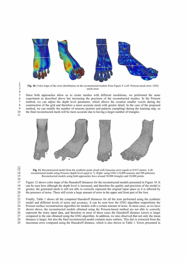
 1 Fig. 10. Color maps of the error distribution on the reconstructed models from Figure 9. Left: Poisson mesh error. GNG 2

mesh error. 3 4

Since both approaches allow us to create meshes with different resolutions, we performed the same 5 experiment as described above but increasing the precision of the reconstructed meshes. In the Poisson 6 method, we can adjust the depth level parameter, which allows the creation smaller voxels during the 7 construction of the grid and therefore a more accurate mesh with greater detail. In the case of the proposed 8 method, we can modify the number of neurons (points) and patterns (sampling) during the learning step, so 9 the final reconstructed mesh will be more accurate due to having a larger number of triangles. 10 11

12 Fig. 11. Reconstructed model from the synthetic point cloud with Gaussian error equals to 0.015 meters. Left: 13

reconstructed model using Poisson (depth level equal to 7). Right: using GNG (10,000 neurons and 500 patterns). 14 Reconstructed models using both approaches have around 30,000 triangles and 10,000 points. 15

16 Figure 12 shows color maps of the Hausdorff distances for the reconstructed models presented in Figure 10. It 17 can be seen how although the depth level is increased, and therefore the quality and precision of the model is 18 greater, the generated mesh is still not able to correctly represent the original input space as it is affected by 19 the presence of noise. There still exists a large amount of error in the upper and front part of the foot. 20 21 Finally, Table 1 shows all the computed Hausdorff distances for all the tests performed using the synthetic 22 model and different levels of noise and accuracy. It can be seen how the GNG algorithm outperforms the 23 Poisson surface reconstruction algorithm for models with a certain amount of noise. In most cases, as we have 24 shown above, the reconstructed models obtained using the Poisson-based method are not able to correctly 25 represent the noisy input data, and therefore in most of these cases the Hausdorff distance (error) is larger 26 compared to the one obtained using the GNG algorithm. In addition, we also observed that not only the mean 27 distance is larger, but also the final reconstructed model contains more outliers. This fact is extracted from the 28 maximum error computed using the Hausdorff distance, which is also shown in Table 1. Errors presented in 29

Table 1 are in millimeters. Furthermore, since the Poisson method does not make it possible to define the 1 number of points for the final reconstructed model and the proposed method does allows the definition of the 2 number of points that the generated model will have, for these experiments, and to establish a fair comparison 3 between both methods, we defined for the GNG method the same number of points as the Poisson algorithm 4 created for different levels of depth, which is the parameter that enable us to define the accuracy of the 5 reconstructed model. 6 7 8

9 Fig. 12. Color maps of the error distribution on the reconstructed models from Figure 11. Left: Poisson mesh. GNG mesh. 10

11 Table. 1. Hausdorff distances (millimeters) from the reconstructed models to the ground truth. 12

13 Method  σ 

Error Points  Min  Max  Mean  RMS 

Poisson  1  5000  0.007333  3.68279  0.87323  0.99457 

GNG  1  5000  0.000004  3.84865  0.29384  0.38677 

Poisson  1  12000  0  17.7058  2.15407  4.29156 

GNG  1  12000  0  3.4955  0.29993  0.38611 

Poisson  1  18000  0.000004  17.698  1.61005  3.17827 

GNG  1  18000  0  3.33448  0.31902  0.41999 

Poisson  1.5  5000  0.000021  17.7057  3.20167  5.048134 

GNG  1.5  5000  0  4.7999  0.39979  0.515214 

Poisson  1.5  12000  0  17.7038  2.19514  3.89758 

GNG  1.5  12000  0.000003  3.69791  0.43041  0.54728 

Poisson  1.5  18000  0.00003  17.7055  2.03972  3.424799 

GNG  1.5  18000  0  4.2719  0.47757  0.635926 

Poisson  3  5000  0.000043  17.7054  2.61422  4.34918 

GNG  3  5000  0  5.54757  0.75227  0.94262 

Poisson  3  12000  0  14.3082  2.57997  3.36485 

GNG  3  12000  0.000002  5.58211  0.66507  0.84519 

Poisson  3  18000  0.000065  14.90595  2.482502  3.143114 

GNG  3  18000  0.000002  5.983467  0.645662  0.837434 

14 15 16

With regard to computational cost, our method is feasible in a modern manufacturing system using general 1 purpose computing platforms. However, in a previous work [40] we designed a GPU-based implementation 2 of the GNG algorithm that speeds up the sequential version several times. The speed-up becomes higher as 3 the number of neurons used for the representation grows. 4 Table 2 shows some reconstructions with a different number of neurons and input patterns with CPU and 5 GPU runtimes and the speed-up obtained with the GPU version with respect to the CPU ones. The GPU used 6 was a GTX 480 NVIDIA graphic card with 480 cores, a global memory of 1.5MB and a bandwidth memory 7 of 177.4 GB/sec. 8

Table. 2. Runtimes and speed up of GPU vs CPU implementation for different GNG versions. 9 10

Neurons  Patterns  CPU Runtime(s)  GPU speed‐up  GPU Runtime (s) 

5000  250  63  3x  21 

12000  350  526  5x  105.2 

18000  500  1448  6x  241.3333333 

11

4.3 Human foot reconstruction: qualitative experiments 12

We finally performed some experiments on 4 different feet acquired using the 3D laser mentioned above. For 13 this experiment we used the 4 feet shown above in the Data Set section. These feet belong to different people 14 and therefore also have different sizes and shapes. As we do not have ground truth information about these 15 feet, we visually analyzed the reconstructed models using the proposed method and the Poisson surface 16 reconstruction algorithm. One disadvantage of the Poisson-based method is that it requires robust normal 17 information for surface reconstruction. If this normal information is not accurate or does not represent the 18 input space well, the final reconstructed model usually presents deformations. 19 20 Figure 13 shows the reconstructed models created using both methods and using different parameters for 21 obtaining meshes with different numbers of triangles and therefore with different precision. Although the 3D 22 reconstructions obtained using the Poisson algorithm could visually appear more regular and with less abrupt 23 changes than the ones obtained by the proposed method, most surfaces created by the Poisson method are 24 approximated and do not correctly represent the input space, changing the original shape of the model. The 25 Poisson algorithm interpolates the input space data and therefore error observed in particular areas also has an 26 important effect in other areas of the final reconstructed model. Figure 14 illustrates this effect. On the left 27 part of the picture it can be seen how Poisson´s algorithm considers the noise in the back part of the foot on 28 the final reconstructed model, generating some protuberances in the back part, while on the right side it can be 29 seen how the GNG algorithm deals with this noisy area by creating a more regular surface on the back part of 30 the foot. 31

Figure 14 shows the difference in the reconstruction of the area of the heel. This area is critical because 32 from it some basic and useful measures in the manufacture of custom footwear are obtained. An erroneous 33 reconstruction of it can make the measurement taken in that area (see Figure 15) such as the heel girth, instep 34 girth or high instep girth defined in [7] differ from the real foot by an excessive number of millimeters, which 35 implies an invalid setting and therefore an erroneous and deficient custom foot will be obtained. 36 37 38

1

2 Fig. 13. Reconstructed models of a real human foot (left) acquired using a 3D scanner. From left to right: reconstructed 3

model using Poisson (around 10,000 faces), using Poisson (around 30,000 faces), using GNG (5,000 neurons and around 4 10,000 faces) and using GNG (14,000 neurons and 30,000 faces). 5

6 7 8

9 Fig. 14. Reconstructed models from real human feet acquired using a 3D scanner. Left: protuberances generated on the 10

back part of the foot using the Poisson method. Right: reconstructed model using the GNG algorithm. It can be seen how 11 GNG allows the creation of more regular surfaces even on areas with a large level of noise. 12

13 14

1 Fig. 15. Different curves whose perimeter measurement are used to manufacture custom footwear. 2

5 CONCLUSIONS 3

New challenges in the footwear industry involve custom manufacturing. The business model based on 4 large sets of pairs organized into feet means population (size) giving way to the production of pairs adjusted 5 to each consumer foot. This new challenge means efforts to accelerate the design process, as opposed to the 6 current scheme which seeks to accelerate the process of mass production. Rapid prototyping is necessary in 7 this new scenario. A bottleneck at this stage is the digitization and subsequent reconstruction of the surface of 8 the foot for the design software which requires accurate and feasible methods for the footwear industry. 9

This article has presented a neural-network-based GNG methodology to reconstruct the surface of the foot, 10 providing greater accuracy than that provided by equally effective and widely used methods such as Marching 11 Cubes. 12

The network obtains a surface representation adapted to the topology of the foot, is tolerant to noise, and 13 eliminates outliers. It also improves the reconstruction in "dark" areas where the scanner does not obtain 14 information, such as the heel and toe areas. 15

Different experiments have been carried out to validate the proposed method: on the one hand we 16 performed a quantitative study using a synthetic foot and adding different levels of noise to the ground truth 17 model. Using the ground truth foot and the one generated by adding noise and some imperfections, we 18 demonstrated that the error produced by our 3D reconstruction method is very low. In addition, our method is 19 compared against the state-of-the-art Poisson surface reconstruction algorithm using the already mentioned 20 synthetic noisy model. On the other hand, data from a 3D laser foot scanner has been reconstructed with our 21 methods and visually compared against results obtained using Poisson surface reconstruction. 22

Although the method has been tested on feet, it is generic and easily extensible to other industrial objects 23 that need to be digitized and reconstructed with accuracy and efficiency requirements. As an extension of this 24 research, we propose to improve the efficiency of the GNG using the inherent parallelism of the algorithm 25 and redesign it to suit multiprocessor platforms such as GPUs. 26

ACKNOWLEDGMENT 1

This work was partially funded by the Spanish Government DPI2013-40534-R grant, supported with Feder 2 funds. The shoe last of footwear used for the experiments have been provided by the Spanish Technological 3 Institute for Footwear Research (INESCOP). Experiments were made possible with a generous donation of 4 hardware from NVIDIA. 5

REFERENCES 6

[1] M.G. Hoy, F.E. Zajac, M.E Gordon. A musculoskeletal model of the human lower extremity: the effect of 7 muscle, tendon, and moment arm on the moment-angle relationship of musculotendon actuators at the hip, 8 knee and ankle. Journal of Biomechanics, 23(2) (1990) 157-169. 9 10 [2] M. Mochimaru, M. Kouchi. Last customization from an individual foot form and design dimensions. 11 Journal of Ergonomics, 43(9) (2000) 1301-1313. 12 13 [3] L. Kos, J. Duhovnik. A system for footwear-fitting analysis. Proceedings of International Design 14 Conference, (2002) 1187-1192. 15 [4] R. Goonetilleke, A. Luximon, K. Tsui. Foot landmarking for footwear customization. Journal of 16 Ergonomics, 46(4) (2003) 364-383. 17 18 [5] J. Leng, R. Du. A deformation method for shoe last customization. Computer Aided Design and 19 Applications, 2(1-4) (2005) 11-18. 20 21 [6] C.S. Wang. An analysis and evaluation of fitness for shoe last and human feet. Journal of Computers in 22 Industry. Elsevier Science Publishers, 61(6) (2010) 532-540. 23 24 [7] M. Davia, A. Jimeno-Morenilla, F. Salas. Footwear bio-modelling: An industrial approach. Computer-25 Aided Design, 45(12), (2013) 1575-1590. 26 27 [8] R. Raffeli, M. Germani. Advanced computer aided design technologies for design automation in footwear 28 industry. International Journal on Interactive Design and Manufacturing, 5(3) (2011) 137-149. 29 30 [9] J.A. Bernabéu, M. Germani, M. Mandolini, M. Mengoni, C. Nester, S. Preece, R. Raffaeli. CAD tools for 31 designing shoe lasts for people with diabetes. Computer-Aided Design, 45(6) (2013) 977-990. 32 33 [10] T. Zahari, M.A. Aris, A. Zulkifli, H. Mohd Hasnun Ariff, S. Nina Nadia. A Low Cost 3D Foot Scanner 34 for Custom-Made Sports Shoes. Advanced Materials Research. (2013). 35 36 [11] H. Edelsbrunner, E.P. Mucke. Three dimensional alpha shapes. ACM Transactions on Graphics (TOG), 37 13(1) (1994) 43-42. 38 39 [12] J.D. Boissonnat. Geometric structures for three-dimensional shape representation. ACM Transactions on 40 Graphics (TOG), 3(4) (1984) 266-286. 41 42 [13] N. Amenta, S. Choi, R.K. Kolluri. The power crust. Proceedings of the sixth ACM symposium on Solid 43 modeling and applications (SMA '01). ACM (2001) 249-266. 44 45

[14] T.K. Dey, S. Goswami. Tight cocone: a water-tight surface reconstructor. Proceedings of the eighth 1 ACM symposium on Solid modeling and applications (SM '03). ACM (2003) 127-134. 2 3 [15] T.K. Dey, S. Goswami. Provable surface reconstruction from noisy samples. In Proc. 20th ACM 4 Sympos. Comput. Geom. (2004). 5 6 [16] B. Mederos, N. Amenta, L. Velho, L.E. De Figueiredo. Surface reconstruction form noisy point clouds. 7 Proceedings of the third Eurographics symposium on Geometry processing. Eurographics Association. (2005) 8 53. 9 10 [17] C.I. Connolly. Cumulative generation of octrees models from range data. In Proceedings, Intl. Conf. 11 Robotics. (1984) 25–32. 12 13 [18] L. Kobbelt, M. Botsch. A survey of point based techniques in computer graphics. Computers & Graphics 14 28, 6 (2004) 801–814. 15 16 [19] A. Jimeno-Morenilla, J. García-Rodriguez, S. Orts-Escolano, M. Davia-Aracil. 3D-based reconstruction 17 using growing neural gas landmark: application to rapid prototyping in shoe last manufacturing. The 18 International Journal of Advanced Manufacturing Technology, 69(1) (2013) 657-668. 19 20 [20] W.E. Lorensen, H.E. Cline. Marching Cubes: A high resolution 3D surface construction algorithm. 21 Proceedings of the 14th annual conference on Computer graphics and interactive techniques (SIGGRAPH 22 '87), 21(4) (1987) 163-169. 23 [21] H. Hoppe. Surface reconstruction from unorganized points. Ph.D. Dissertation. University of 24 Washington. (1994). 25 26 [22] J.C. Carr, R.K. Beatson, J.B. Cherrie, T.J. Mitchell, W.R. Fright, B.C. McCallum, T.R. Evans. 27 Reconstruction and representation of 3d objects with radial basic functions. Proceedings of the 28th annual 28 conference on Computer graphics and interactive techniques (SIGGRAPH '01). ACM (2001) 67-76. 29 30 [23] C. Shen, J.F. O'Brien, J.R. Shewchuk. Interpolating and approximating implicit surfaces from polygon 31 soup. ACM Transactions on Graphics (TOG), 23(3) (2004) 896-904. 32 33 [24] S. Fleishman. D. Cohen-Or, C.T. Silva. Robust moving least squares fitting with sharp features. ACM 34 Transactions on Graphics (TOG), 24(3) (2005) 544-552. 35 36 [25] C. Walder, B. Schoelkopf, O. Chapelle. Implicit surface modelling with a globally regularised basis of 37 compact support. Proceedings of the Eurographics symposium on Computer Graphics. Eurographics 38 Association, 25(3) (2006) 635-644. 39 40 [26] M. Kazhdan, M. Bolitho, H. Hoppe. Poisson surface reconstruction. Proceedings of the fourth 41 Eurographics symposium on Geometry processing (SGP '06). Eurographics Association (2006) 61-70. 42 43 [27] C.L. Wang. Incremental reconstruction of sharp edges on mesh surfaces. Journal of Computer-aided 44 design, 38(6) (2006) 789-702. 45 46 [28] H.R. Davies, J.C. Twining, F.T. Cootes, C.J. Waterton, J.C. Taylor. A minimum description length 47 approach to statistical shape modeling. IEEE Transaction on Medical Imaging, 21(5) (2002) 525–537. 48 49 [29] E. Fatemizadeh, C. Lucas, H. Soltania-Zadeh. Automatic landmark extraction from image data using 50 modified growing neural gas network. IEEE Transactions on Information Technology in Biomedicine, 7(2) 51 (2003) 77–85. 52 53

[30] N. Ansari, J. Delp. On detecting dominant points. Pattern Recognit., 26 (1991) 441–451. 1 2 [31] C.-H. The, R.T. Chin. On the detection of dominant points on digital curves. IEEE Trans. Pattern Anal. 3 Machine Intell.,11 (1989). 4 5 [32] S.-C. Pei, C.-N. Lin. The detection of dominant points on digital curves by scale-space filtering. Pattern 6 Recognit., 25 (1992) 1307–1314. 7 8 [33] B. Fritzke. A Growing Neural Gas Network Learns Topologies. In Advances in Neural Information 9 Processing Systems 7, G. Tesauro, D.S. Touretzky and T.K. Leen (eds.), MIT Press, (1995) 625-632. 10 11 [34] T. Martinetz, K. Shulten. Topology Representing Networks. Neural Networks, 7(3) (1994) 507-522. 12 13 [35] J. Garcia-Rodriguez, A. Angelopoulou, A.Psarrou. Growing Neural Gas (GNG): A Soft Competitive 14 Learning Method for 2D Hand Modelling. IEICE Trans. Inf. & Syst. E89-D(7) (2006). 15 16 [36] A. Angelopoulou, A., Psarrou, J. Garcia-Rodriguez, K. Revett. Automatic Landmarking of 2D Medical 17 Shapes Using the Growing Neural Gas Network. In proc. Of the IEEE Workshop on Computer Vision for 18 Biomedical Image Applications, CVBIA 2005, LNCS 3765 (2005) 210-219. 19 20 [37] R.B. Rusu, S. Cousins. 3D is here: Point Cloud Library (PCL). In proceedings of the IEEE International 21 Conference on Robotics and Automation (ICRA), Shangai, China (2011). 22 23 [38] M.P. Dubbuison, A.K. Jain. A Modified Hausdorff Distance for Object Matching, In Proceedings of the 24 International Conference on Pattern Recognition, Jerusalem, Israel, (1994) 566-568. 25 26 [39] P. Cignoni, C. Rocchini, R. Scopigno. Metro: measuring error of simplified surfaces. Computer Graphics 27 Forum. 17(2) (1998) 167-174. 28 29 [40] S. Orts, J. Garcia-Rodriguez, D. Viejo, M. Cazorla, V. Morell. GPGPU implementation of growing 30 neural gas: Application to 3D scene reconstruction. J. Parallel Distrib. Comput. 7 (2012) 1361–1372. 31 32 33