Geosci. Model Dev., 4, 435–449, 2011www.geosci-model-dev.net/4/435/2011/doi:10.5194/gmd-4-435-2011© Author(s) 2011. CC Attribution 3.0 License.

GeoscientificModel Development

Automated continuous verification for numerical simulation

P. E. Farrell1, M. D. Piggott1,2, G. J. Gorman1, D. A. Ham1,2, C. R. Wilson3, and T. M. Bond1

1Applied Modelling and Computation Group, Department of Earth Science and Engineering, Imperial College London,SW7 2AZ, UK2Grantham Institute for Climate Change, Imperial College London, London, SW7 2AZ, UK3Lamont-Doherty Earth Observatory, Columbia University, New York, USA

Received: 23 August 2010 – Published in Geosci. Model Dev. Discuss.: 29 September 2010Revised: 6 May 2011 – Accepted: 10 May 2011 – Published: 16 May 2011

Abstract. Verification is a process crucially important for thefinal users of a computational model: code is useless if its re-sults cannot be relied upon. Typically, verification is seen asa discrete event, performed once and for all after develop-ment is complete. However, this does not reflect the realitythat many geoscientific codes undergo continuous develop-ment of the mathematical model, discretisation and softwareimplementation. Therefore, we advocate that in such casesverification must be continuous and happen in parallel withdevelopment: the desirability of their automation follows im-mediately. This paper discusses a framework for automatedcontinuous verification of wide applicability to any kind ofnumerical simulation. It also documents a range of test casesto show the possibilities of the framework.

1 Introduction

Since the development of the computer, numerical simula-tion has become an integral part of many scientific and tech-nical enterprises. As computational hardware becomes evercheaper, numerical simulation becomes more attractive rel-ative to experimentation. Much attention is paid to the de-velopment of ever more efficient and powerful algorithmsto solve previously intractable problems (Trefethen, 2008).However, in order to be useful, the user of a computationalmodel must have confidence that the results of the numeri-cal simulation are an accurate proxy for reality. A rigoroussoftware quality assurance system is usually a requirementfor any deployment to industry, and should be a requirementfor any scientific use of a model. Catastrophic accidents suchas the Sleipner platform accident, in which an offshore plat-form collapsed due to failures in finite element modelling,

Correspondence to:D. A. Ham(david.ham@imperial.ac.uk)

underscore the importance of such efforts. More recently,the controversy surrounding the leaking of emails from theClimate Research Unit at the University of East Anglia un-derlines the importance of rigorous and auditable testing ofscientific software. Failure to properly establish the prove-nance of simulation results risks undermining public confi-dence in science.

This paper has two purposes. First, it documents and advo-cates best practice in the automatic verification of scientificcomputer models. Second, it documents the particular sys-tem in place for Fluidity-ICOM enabling users of publishedFluidity-ICOM results to understand the verification processbehind that particular model.

1.1 Verification and validation

Verification and validation provide the framework for estab-lishing the usefulness of a computational model for a partic-ular physical situation. Verification assesses the differencebetween the results produced by the code and the mathemat-ical model. Validation determines if a mathematical modelrepresents the physical situation of interest, i.e. the abilityof the model to accurately reproduce experimental data. Ifthe computational model describes the mathematical modelwell, and the mathematical model relates well to the physi-cal world, then the computational model also relates well tothe physical world (Babuska and Oden, 2004). Philosoph-ically, it is impossible to ever assert with absolute certaintythat a code will accurately simulate a given physical situationof interest after verifying a finite set of tests (Popper, 1959;Howden, 1976); however, it is clear that a code which is cor-roborated by having passed the most stringent tests availableis surely more useful than a code which has not been scruti-nised at all (Babuska and Oden, 2004).

Verification divides into two parts. Code verification isthe process of ensuring, to the best degree possible, thatthere are no coding errors affecting the implementation of the

Published by Copernicus Publications on behalf of the European Geosciences Union.

436 P. E. Farrell et al.: Automated continuous verification for numerical simulation

discretisation. Code verification assesses the difference be-tween the code and the discretised model. The other compo-nent of model verification is solution verification, assessingthe difference between the discretised model and the math-ematical model. Code verification deals with software en-gineering, while solution verification deals with a posteriorierror estimation.

An important but subtle distinction between verificationand validation is that validity is a property of the algorithmwhich the model code implements rather than a propertyof the code itself. To the extent to which validation testshave established the validity of an algorithm, the repetitionof those tests does not further establish validity. If a modelwhich has been validated fails to perform as expected due toa change in the code, this is averification error.

Often, undergoing verification is seen as a discrete event,happening after the computational model is completed. Yetmany computational models that are used for practical appli-cations are also under active software development; it doesnot make sense to assert that the code has been verified, whenthe code has changed since the verification was performed.In principle, whenever the code is changed, verification mustbe applied to the new revision, for any previous results areirrelevant. We therefore advocate the view that verificationmust be treated as a continuous process, happening along-side both software development and usage. This is the onlyway to ensure that the entire modelling effort stays correct asit is developed.

This poses a difficulty. These processes are generally seento be time-consuming, uninteresting work. Therefore, theyshould be automated in order to minimise the amount ofmanual intervention required in the scrutiny of the newly-changed code. InKnupp et al.(2007), it is implicitly arguedthat code verification takes too much effort to perform onthe very latest version, and is thus relegated to release candi-dates; however, by automating the process, we have achievedgreat success in applying code verification to a codebase thatchanges daily. This philosophy is widespread in the soft-ware engineering community (Adrion et al., 1982), but is notyet the generally accepted practice among the scientific mod-elling community. We discuss a framework for automatedcontinuous verification with particular suitability to numer-ical models. The framework is of wide applicability to anynumerical model, although emphasis is placed on modellingin a geoscientific context.

1.2 Other automated verification of geoscientific models

We do not claim that this is the first invention of continu-ous code verification. Several large, successful geoscientificmodels undergo similar efforts. The MIT general circulationmodel (Marshall et al., 1997) has an automated system thatruns a verification suite on a variety of different machines.The summary page is available athttp://mitgcm.org/public/testing.html. The Unified Model developed by the UK Met

Office (Davies et al., 2005) also has an automated nightlyverification system, as documented inEasterbrook and Johns(2009). Other research groups have developed suites of testssuitable for use in automated verification; these researchersmay well have automated the process, although the authorswere unable to find any information about any such automa-tion on their websites. The Modular Ocean Model developedat Princeton (Griffies et al., 2004) documents an extensivecollection of verification test cases in their manual (Griffies,2009). The Regional Ocean Modeling System developed atRutgers University (Song and Haidvogel, 1994) lists a col-lection of test cases athttps://www.myroms.org/wiki/index.php/TestCases. Other large, successful projects do not ap-pear to regard verification as an ongoing process. The con-tract setting up the consortium to develop the NEMO oceanmodel (Madec et al., 1998) states that the (quote) “testing andrelease of new versions” happens “typically once or twicea year” (NEMO Consortium, 2008). The SLIM Ice-Oceanmodel developed at the Universite catholique de Louvain(White et al., 2008) states that (quote) “we ran as few simplis-tic, highly-idealised test cases as possible. Instead, wheneverpossible, we tested the model against realistic flows, albeitoften simple ones” (Deleersnijder et al., 2010). As realisticsimulations are typically too expensive to run continuously,this suggests that no automated continuous verification sys-tem is in place.

This brief survey highlights two important points. Thefirst is that even among large and successful modelling ef-forts, the practice of automated, continuous verification isfar from universal. Note that the projects examined all havelarge development teams and may have professional IT sup-port. This is very atypical of geoscientific modelling in gen-eral: the more usual case is of in-house development in asmall research group with code passed informally from onegeneration of PhD students and post-docs to the next.

The second point is that even the large, well-resourcedprojects do not typically publish their code verification prac-tices in the formal, peer-reviewed literature. As noted above,the authors feel that it is important in maintaining public con-fidence in simulation results that the provenance, includingverification processes, of those results is well established. Itis therefore to be hoped that the developers of other modelswill follow this lead and publish their verification processes.

1.3 Fluidity-ICOM

Although the framework presented here is applicable to anynumerical model, it is useful to present particular exam-ples. For this we will use the example of Fluidity-ICOM,the primary software package to which this particular frame-work has been applied. Fluidity is a finite element, adap-tive mesh fluid dynamics simulation package. It is capa-ble of solving the full Navier-Stokes equations in compress-ible or incompressible form, or the Boussinesq equations. Itis equipped with numerous parameterisations for sub-grid-

Geosci. Model Dev., 4, 435–449, 2011 www.geosci-model-dev.net/4/435/2011/

P. E. Farrell et al.: Automated continuous verification for numerical simulation 437

scale processes and has embedded models for phenomena asvaried as ocean biology, traffic pollution, radiation transportand porous media. Fluidity supports a number of differentfinite element discretisations and is applied to flow problemsin a number of scientific and engineering domains including,in particular, ocean flows. In this last context it is known asthe Imperial College Ocean Model (Fluidity-ICOM) and thisis the name we will use here. For particular information onFluidity-ICOM as an ocean model, the reader is referred toPiggott et al.(2008).

While verification is essential for all scientific computersoftware, the complexity and wide applicability of theFluidity-ICOM makes this a particularly challenging andcritical requirement. The model is developed by severaldozen scientists at a number of different institutions and thereare approximately 15 commits (changes to the model) on anaverage work day. In the absence of constant verification,development would be impossible.

2 Verification tests

There are two general strategies to inspect the source code ofa computational model. Static analysis involves (usually au-tomated) inspection of the source code itself for issues suchas uninitialised variables, mismatched interfaces and off-by-one array indexing errors. Dynamic analysis involves run-ning the software and comparing the output (some functionalof the solution variables) to an expected output. The sourceof the expected output determines the rigour and purpose ofthe test. Various sources are possible:

– The simplest and least rigorous is to compare the outputto previous output; this tests code stability, not code cor-rectness, but can still be useful (Oberkampf and Atru-cano, 2002).

– The expected output could be output previously pro-duced by the code that has been examined by an expertin the field. While flawed, asserting the plausibility ofthe results is better than nothing at all. The test in thiscase can again be that the output has not changed fromprevious runs, except where expected.

– The expected output could come from a high-resolutionsimulation from another verified computational modelof the same discretisation. However, analytical solu-tions are to be preferred as they remove the possibilityof common algorithmic error among the implementa-tions.

– The expected output could come from an analytical so-lution. The test in this case could be the quantificationof error in the simulation or numerically computing therate of convergence to the true solution as some discreti-sation parameter (h, 1t , ...) tends to 0. Comparing the

obtained rate of convergence against the theoreticallypredicted rate of convergence is generally consideredthe most powerful test available for ensuring that thediscretised model is implemented correctly, as it is verysensitive to coding errors (Roache, 2002; Knupp et al.,2007).

– The analytical solution could come from the methodof manufactured solutions (Salari and Knupp, 2000;Roache, 2002). This method involves adding in extrasource terms to the governing equations being solved inorder to engineer an equation whose solution is known.It is a general and powerful technique for generating an-alytical solutions for use in error quantification or con-vergence analyses.

– Once the code verification tests have completed, solu-tion verification for a library of simulations may takeplace. The functional could be some a posteriori esti-mate of the discretisation error, and the expected outputthat it is below a given tolerance. Formally, this solutionverification step is only necessary when the discretisa-tion has changed.

– The final source of verification is to re-run previous val-idation tests. For this purpose, the expected output is de-rived from a physical experiment. Again, the test couldassert that the rate of convergence to the physical re-sult is the same as theoretically predicted. Comparingoutput to experimental data asserts the applicability ofboth the computational and mathematical models to thephysical world. It is to be emphasised that model verifi-cation should happen before model validation, for other-wise the error introduced in the mathematical modellingcannot be distinguished from discretisation or codingerrors (Babuska and Oden, 2004). However once a val-idation test has been passed, the repetition of that testcan be used to verify the model after subsequent codechanges.

In general, atest caseis a set of input files, a set of com-mands to be run on those input files, some functionals ofthe output of these commands to be computed, and somecomparisons against independent data of those functionals.While the purpose and level of rigour of the test changes withthe source of the comparison data, this is irrelevant for the ex-ecution of the test itself. Indeed, the generality of this viewis a great benefit to the design of the framework: code stabil-ity tests, code verification and solution verification can all beperformed by the same system. Note that this conception ofa test case encompasses both static and dynamic analysis: instatic analysis, the command to be run is the analysis tool; indynamic analysis, the command to be run is the model itself.

www.geosci-model-dev.net/4/435/2011/ Geosci. Model Dev., 4, 435–449, 2011

438 P. E. Farrell et al.: Automated continuous verification for numerical simulation

2.1 Verification as a continuous process

In reality, most computational models are both in produc-tion use by end-users and undergoing continual development.Even if the verification procedure has been passed for a pre-vious revision, it does not necessarily mean that the next re-vision of the computational model will also pass. New de-velopment can and does introduce new coding errors. There-fore, verification must be seen as a continuous process: itmust happen alongside the software development and de-ployment. Integrating this process alongside software devel-opment greatly eases the burden of deploying stable, workingreleases to end users.

Regarding verification as a continuous process has manybenefits for the parallel process of software development. Asnew features are added, feedback is immediately availableabout the impact of these changes to the accuracy of the com-putational model; since coding errors are detected soon afterthey are introduced, they are easier to fix as the programmeris still familiar with the newly introduced code. Furthermore,as software development teams become large, it can be dif-ficult to predict the impact of a change to one subroutine toother users of the model; if those other uses of the softwareare exercised as part of the continuous verification processthen unintended side-effects can be detected early and fixed.Since the code is run continuously to check for correctness,other metrics can be obtained at the same time: for example,profiling information can be collected to detect any efficiencychanges in the implementation.

2.2 Verification should be automated

Verifying every change to a code base as part of a continuouscode verification procedure is laborious and repetitive. It is atherefore natural candidate for automation.

Automating the process of code verification means thatchecking for correctness can be performed simultaneouslyon multiple platforms with multiple compilers, platforms towhich an individual developer may not have access. It alsomeans that more tests can be run than would be practical fora single human to run; these tests can therefore check morecode paths through the software, and can be more pedanticand time-consuming than a human would tolerate. In prac-tice, without automation, the amount of continuous code ver-ification is limited to the problems of immediate interest tothe currently active development projects.

2.3 The limitations of testing

It has been noted elsewhereOreskes et al.(1994) that com-plex geoscientific models such as GCMs may be formally un-verifiable simply because they do not constitute closed math-ematical systems. Aspects of these models, particularly pa-rameterisations, may be difficult to formulate analytic solu-tions for and may not, in fact, converge under mesh refine-

ment. Nonetheless, individual components of models con-sidered in isolation, for example the dynamic core or an indi-vidual parameterisation, must have well-defined and testablemathematical behaviour if there is to be any confidence inthe model output at all. If there is to be any confidence inthe output of a formally unverifiable model, it is surely anecessary condition that each verifiable component passesverification. The methodology explained here is thereforeuseful in at least this context. The automated verificationof code stability (i.e. that the model result does not unex-pectedly change) must also be regarded as a key tool in theverification of the most complex models.

3 A framework for automated continuous verification

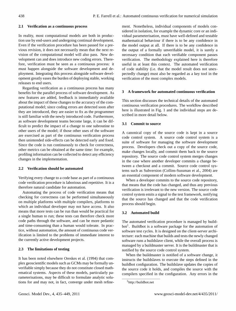
This section discusses the technical details of the automatedcontinuous verification procedures. The workflow describedhere is illustrated in Fig.1 and the individual steps are de-scribed in more detail below.

3.1 Commit to source

A canonical copy of the source code is kept in a sourcecode control system. A source code control system is asuite of software for managing the software developmentprocess. Developers check out a copy of the source code,make changes locally, and commit them back to the sourcerepository. The source code control system merges changesin the case where another developer commits a change be-tween a checkout and a commit. Source code control sys-tems such as Subversion (Collins-Sussman et al., 2004) arean essential component of modern software development.

When a developer commits to the source code repository,that means that the code has changed, and thus any previousverification is irrelevant to the new version. The source codecontrol system emits a signal to the test framework, notifyingthat the source has changed and that the code verificationprocess should begin.

3.2 Automated build

The automated verification procedure is managed by build-bot1. Buildbot is a software package for the automation ofsoftware test cycles. It is designed on the client-server archi-tecture: each machine that builds and tests the newly changedsoftware runs a buildslave client, while the overall process ismanaged by a buildmaster server. It is the buildmaster that isnotified by the source code control system.

When the buildmaster is notified of a software change, itinstructs the buildslaves to execute the steps defined in thebuildbot configuration. The buildslave updates the copies ofthe source code it holds, and compiles the source with thecompilers specified in the configuration. Any errors in the

1http://buildbot.net

Geosci. Model Dev., 4, 435–449, 2011 www.geosci-model-dev.net/4/435/2011/

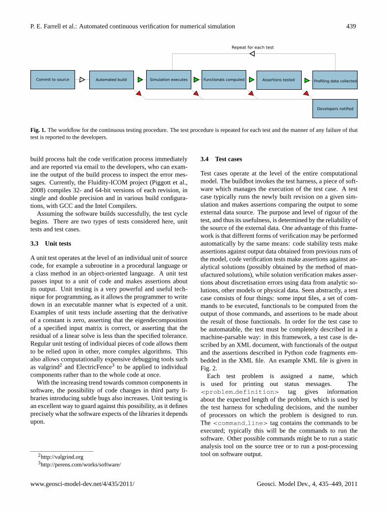
P. E. Farrell et al.: Automated continuous verification for numerical simulation 439

Automated build Simulation executesCommit to source Assertions tested Profiling data collected

Developers notified

Functionals computed

Repeat for each test

Fig. 1. The workflow for the continuous testing procedure. The test procedure is repeated for each test and the manner of any failure of thattest is reported to the developers.

build process halt the code verification process immediatelyand are reported via email to the developers, who can exam-ine the output of the build process to inspect the error mes-sages. Currently, the Fluidity-ICOM project (Piggott et al.,2008) compiles 32- and 64-bit versions of each revision, insingle and double precision and in various build configura-tions, with GCC and the Intel Compilers.

Assuming the software builds successfully, the test cyclebegins. There are two types of tests considered here, unittests and test cases.

3.3 Unit tests

A unit test operates at the level of an individual unit of sourcecode, for example a subroutine in a procedural language ora class method in an object-oriented language. A unit testpasses input to a unit of code and makes assertions aboutits output. Unit testing is a very powerful and useful tech-nique for programming, as it allows the programmer to writedown in an executable manner what is expected of a unit.Examples of unit tests include asserting that the derivativeof a constant is zero, asserting that the eigendecompositionof a specified input matrix is correct, or asserting that theresidual of a linear solve is less than the specified tolerance.Regular unit testing of individual pieces of code allows themto be relied upon in other, more complex algorithms. Thisalso allows computationally expensive debugging tools suchas valgrind2 and ElectricFence3 to be applied to individualcomponents rather than to the whole code at once.

With the increasing trend towards common components insoftware, the possibility of code changes in third party li-braries introducing subtle bugs also increases. Unit testing isan excellent way to guard against this possibility, as it definesprecisely what the software expects of the libraries it dependsupon.

2http://valgrind.org3http://perens.com/works/software/

3.4 Test cases

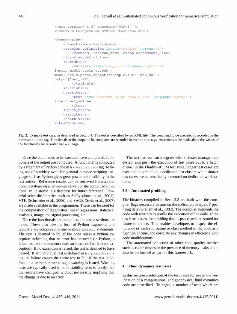
Test cases operate at the level of the entire computationalmodel. The buildbot invokes the test harness, a piece of soft-ware which manages the execution of the test case. A testcase typically runs the newly built revision on a given sim-ulation and makes assertions comparing the output to someexternal data source. The purpose and level of rigour of thetest, and thus its usefulness, is determined by the reliability ofthe source of the external data. One advantage of this frame-work is that different forms of verification may be performedautomatically by the same means: code stability tests makeassertions against output data obtained from previous runs ofthe model, code verification tests make assertions against an-alytical solutions (possibly obtained by the method of man-ufactured solutions), while solution verification makes asser-tions about discretisation errors using data from analytic so-lutions, other models or physical data. Seen abstractly, a testcase consists of four things: some input files, a set of com-mands to be executed, functionals to be computed from theoutput of those commands, and assertions to be made aboutthe result of those functionals. In order for the test case tobe automatable, the test must be completely described in amachine-parsable way: in this framework, a test case is de-scribed by an XML document, with functionals of the outputand the assertions described in Python code fragments em-bedded in the XML file. An example XML file is given inFig. 2.

Each test problem is assigned a name, whichis used for printing out status messages. The<problem definition > tag gives informationabout the expected length of the problem, which is used bythe test harness for scheduling decisions, and the numberof processors on which the problem is designed to run.The <command line > tag contains the commands to beexecuted; typically this will be the commands to run thesoftware. Other possible commands might be to run a staticanalysis tool on the source tree or to run a post-processingtool on software output.

www.geosci-model-dev.net/4/435/2011/ Geosci. Model Dev., 4, 435–449, 2011

440 P. E. Farrell et al.: Automated continuous verification for numerical simulation

<?xml version="1.0" encoding="UTF-8" ?><!DOCTYPE testproblem SYSTEM "testcase.dtd">

<testproblem ><name>Example test </name><problem_definition length= "medium" nprocs= "1" >

<command_line >run_model example </command_line></problem_definition><variables >

<variable name="max_val" language= "python" >import model_tools output =model_tools.parse_output("example.out") max_val =output[’max_val’]

</variable></variables><pass_tests >

<test name="Maximum value equals one" language= "python" >assert max_val == 1

</test></pass_tests><warn_tests ></warn_tests>

</testproblem>

Fig. 2. Example test case, as described in Sect.3.4. The test is described by an XML file. The command to be executed is recorded in thecommand line tag. Functionals of the output to be computed are recorded invariable tags. Assertions to be made about the values ofthe functionals are recorded intest tags.

Once the commands to be executed have completed, func-tionals of the output are computed. A functional is computedby a fragment of Python code in a<variable > tag. Mak-ing use of a widely available general-purpose scripting lan-guage such as Python gives great power and flexibility to thetest author. Reference results can be retrieved from a rela-tional database on a networked server, or the computed func-tional value stored in a database for future reference. Pow-erful scientific libraries such as SciPy (Jones et al., 2001),VTK (Schroeder et al., 2006) and SAGE (Stein et al., 2007)are made available to the programmer. These can be used forthe computation of diagnostics, linear regressions, statisticalanalyses, image and signal processing, etc.

Once the functionals are computed, the test assertions aremade. These also take the form of Python fragments, andtypically are composed of one or moreassert statements.The test is deemed to fail if the code raises a Python ex-ception indicating that an error has occurred (in Python, afailed assert statement raises anAssertionError ex-ception). If no exception is raised, the test is deemed to havepassed. If an individual test is defined in a<pass test >

tag, its failure causes the entire test to fail; if the test is de-fined in a<warn test > tag, a warning is issued. Warningtests are typically used in code stability tests to notify thatthe results have changed, without necessarily implying thatthe change is due to an error.

The test harness can integrate with a cluster managementsystem and push the execution of test cases out to a batchqueue. In the Fluidity-ICOM test suite, longer test cases areexecuted in parallel on a dedicated test cluster, while shortertest cases are automatically executed on dedicated worksta-tions.

3.5 Automated profiling

The binaries compiled in Sect.3.2 are built with the com-piler flags necessary to turn on the collection ofgprof pro-filing data (Graham et al., 1982). The compiler augments thecode with routines to profile the execution of the code. If thetest case passes, the profiling data is processed and stored forfuture reference. This enables developers to inspect the ef-ficiency of each subroutine or class method of the code as afunction of time, and correlate any changes in efficiency withcode modifications.

The automated collection of other code quality metricssuch as cache misses or the presence of memory leaks couldalso be performed as part of this framework.

4 Fluid dynamics test cases

In this section a selection of the test cases for use in the ver-ification of a computational and geophysical fluid dynamicscode are described. To begin, a number of tests which are

Geosci. Model Dev., 4, 435–449, 2011 www.geosci-model-dev.net/4/435/2011/

P. E. Farrell et al.: Automated continuous verification for numerical simulation 441

suitable for use with a standard fluid dynamics model aredescribed; this is followed by a number of tests suitable formodels which incorporate buoyancy and Coriolis effects, forexample geophysical fluid dynamics codes and ocean mod-els. Note that for the problems presented here the modelhas been set up so as to optimise the efficiency of the test,i.e. to give rigorous checks on the code in minimal compu-tational time, and not necessarily to optimise the accuracy ofthe overall calculation or of the particular metric being used.

The test cases presented here are selected to illustrate arange of problem formulations and test statistics. It is notintended to be a comprehensive list of the tests required ofa particular class of model: the actual test suite employedby Fluidity-ICOM, for example, contains well in excess ofthree hundred tests. The first two tests shown here employthe method of manufactured solutions to create new analyticsolutions as test comparators. The lid-driven cavity and lockexchange tests exemplify the use of the results of other mod-els run at high resolution as a benchmark while Stommel’swestern boundary current is an example of a well-known an-alytic result used as a test case.

The model being tested here uses finite element discreti-sation methods on tetrahedral or hexahedral elements inthree dimensions and triangular or quadrilateral elements intwo dimensions. The underlying equations considered inthe tests presented here include the advection-diffusion ofscalar fields, the Navier-Stokes equations, and the Boussi-nesq equations with buoyancy and Coriolis terms included.The model has the ability to adapt the mesh dynamically inresponse to evolving solution fields. For background to themodel seePain et al.(2005); Piggott et al.(2008). For anoverview of CFD validation and verification, seeOberkampfet al.(1998); Stern et al.(2001).

4.1 Computational fluid dynamics examples

4.1.1 The method of manufactured solutions:tracer advection

To test the implementation of the advection-diffusion andNavier-Stokes equations spatial convergence tests are per-formed using the method of manufactured solutions (MMS,Roache, 2002). MMS provides an easy way of generating an-alytical solutions against which to verify model code. A suf-ficiently smooth desired analytical solution is designed anda suitable source term added to the right hand side to en-sure the validity of the equation. The source is calculated bysubstituting the desired analytical solution in the underlyingdifferential equation.

The numerical equation is then solved on a sequence ofsuccessively finer meshes. The solution on each of these isthen compared to the known exact solution and the order ofconvergence compared to the expected order for that method.When convergence of the solution is not seen, it is an excel-lent indicator of an error in the model code or the numerical

formulation. MMS has been shown to be highly effective atfinding such problems (Salari and Knupp, 2000) and contin-uous monitoring of the results through an automated systemallows errors that affect the order of convergence to be im-mediately noticed.

To test tracer advection-diffusion the desired analytical so-lution is taken as:

T (x,y,t) = sin(25xy)−2y/x1/2, (1)

while a prescribed velocity field,u = (u,v), is given by

u = sin(5(x2

+y2))

, v = cos(3(x2

−y2))

. (2)

The source term,S, is calculated symbolically usingSAGE (Stein et al., 2007) by substitutingT andu into theadvection-diffusion equation:

S =∂T

∂t+u ·∇T −κ∇

2T ,

=

(25ycos(25xy)+y/x3/2

)sin(5(y2

+x2))

+

(25xcos(25xy)−2/x1/2

)cos

(3(x2

−y2))

+κ(625(x2

+y2)sin(25xy)+3y/(2x5/2))

.

The computational domain is 0.1≤ x ≤ 0.6; −0.3≤ y ≤

0.1 and is tessellated with a uniform unstructured Delaunaymesh of triangles with characteristic mesh spacing ofh inthex andy directions. The analytical solution (Eq.1) is usedto define Dirichlet boundary conditions along the inflowinglower and left boundaries while its derivative is used to defineNeumann boundary conditions on the remaining sides. Boththe boundary conditions and source term are defined throughPython functions defined in the Fluidity-ICOM preprocessor(Ham et al., 2009), where the diffusivity,κ, is taken as 0.7.

As we are performing a spatial convergence test, the de-sired solution is temporally invariant. However, the equationcontains a time derivative and requires an initial condition.This is set to zero everywhere leading to a numerical solu-tion that varies through time. The simulation is terminatedonce this reaches a steady state (to a tolerance of 10−10 inthe infinity norm).

Once a steady state has been obtained on all meshes theconvergence analysis may be performed. Given the error,E,on two meshes, with characteristic mesh spacingh1 andh2for example:

Eh1 ≈ Chcp

1 , (3)

Eh2 ≈ C

(h1

r

)cp

, (4)

whereC is a constant discretisation specific factor indepen-dent of the mesh,cp is the order of convergence of themethod andr is the refinement ratio (r = 2 in this case), thenthe ratio of errors is given by:

Eh1

Eh2

≈

(Ch

cp

1

Chcp

1

)rcp = rcp , (5)

www.geosci-model-dev.net/4/435/2011/ Geosci. Model Dev., 4, 435–449, 2011

442 P. E. Farrell et al.: Automated continuous verification for numerical simulation

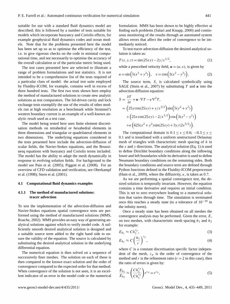
Fig. 3. From left to right: source term (Eq.3) for the method of manufactured solutions advection-diffusion test case, the numerical solutioncalculated using a piecewise-linear Galerkin discretisation, the absolute difference between the analytical and numerical solutions, the meshesused to compute the previous images with average mesh spacings,h, of 0.08 (top) and 0.01 (bottom).

and the order of convergence can be calculated as:

cp ≈ logr

(Eh1

Eh2

). (6)

This can then be compared to the expected order of conver-gence for a particular method.

Several model configurations and discretisations are usedin the full testing suite. Here, the results of a first-order up-winding control volume (CV) discretisation and a second-order piecewise-linear Galerkin (P1) discretisation are pre-sented. In both cases the Crank-Nicolson method is used todiscretise in time. Table1 demonstrates that the expected or-der of spatial convergence, or better, is achieved for both dis-cretisations. Figure3 shows the source term, the numericalsolution using the P1 discretisation, the absolute differencebetween this and the analytical solution at steady state andmeshes with average nodal spacings,h, of 0.08 and 0.01.

4.1.2 The method of manufactured solutions:Navier-Stokes equations

The method of manufactured solutions can also be used totest more complicated sets of equations involving multiplecoupled prognostic fields, such as the Navier-Stokes equa-tions. Initially an incompressible, smooth and divergencefree desired velocity field,u = (u,v) is considered:

u = sin(x)cos(y), v = −cos(x)sin(y), (7)

along with a desired pressure,p:

p = cos(x)cos(y). (8)

These are substituted into the momentum equations, withtensor-form viscosity, using SAGE (Stein et al., 2007) to de-rive the required momentum source:

S = ρ∂u

∂t+ρu ·∇u−µ∇

2u+∇p

=

ρ(cos(x)sin(x)sin2(y)+cos(x)sin(x)cos2(y))

+2µsin(x)cos(y)−sin(x)cos(y)

ρ(cos(y)sin(y)sin2(x)+cos(y)sin(y)cos2(x))

−2µcos(x)sin(y)−cos(x)sin(y)

The incompressible Navier-Stokes equations are then

solved in the computational domain 0≤ x ≤ π ; 0 ≤ y ≤ π

tessellated using an unstructured Delaunay mesh of triangles.Velocity is discretised using a piecewise-quadratic Galerkindiscretisation while pressure uses piecewise-linear elements(the Taylor-Hood element pair). Strong Dirichlet boundaryconditions for velocity are provided on all sides of the do-main using the desired solution while pressure has naturalhomogeneous Neumann boundary conditions enforced. Boththe strong boundary conditions and source term are definedthrough Python functions defined in the Fluidity-ICOM pre-processor (Ham et al., 2009), while the density,ρ, and vis-cosity,µ, are taken as 1.0 and 0.7 respectively.

Table2 presents the convergence results for velocity andpressure on a series of unstructured meshes with successivelysmaller average mesh spacings. For both velocity and pres-sure the expected order of convergence, or better, is observed.

Further variables may be introduced by considering thefully compressible Navier-Stokes equations with a divergentdesired velocity field:

Geosci. Model Dev., 4, 435–449, 2011 www.geosci-model-dev.net/4/435/2011/

P. E. Farrell et al.: Automated continuous verification for numerical simulation 443

Table 1. Spatial order of convergence results for the method of manufactured solutions advection-diffusion test case described in Sect.4.1.1.The difference between the analytical and numerical solutions using a first-order control volume (CV) discretisation and a second-orderpiecewise-linear Galerkin (P1) discretisation are calculated in theL2 norm. The ratio between these on two spatial mesh resolutions,h1andh2, are used to estimate the order of spatial convergence of the model for this problem. The expected order of convergence, or better, isobserved for both spatial discretisations.

h1 → h2 0.08→ 0.04 0.04→ 0.02 0.02→ 0.01 0.01→ 0.005

cp (CV) 2.42 2.00 1.43 0.97cp (P1) 2.03 1.91 2.08 2.12

Table 2. Spatial order of convergence results for the method ofmanufactured solutions incompressible Navier-Stokes test case de-scribed in Sect.4.1.2. The difference between the analytical and nu-merical solutions using a piecewise-quadratic velocity,(u,v), and apiecewise-linear pressure,p, Galerkin discretisation are calculatedin theL2 norm. The ratio between these on two spatial mesh reso-lutions,h1 andh2, are used to estimate the order of spatial conver-gence of the model for this problem. The expected order of conver-gence is observed for all variables.

h1 → h2 0.32→ 0.16 0.16→ 0.08 0.08→ 0.04

cp (u) 3.18 3.03 2.96cp (v) 3.04 2.01 3.04cp (p) 2.27 2.01 1.98

u = sin(x2+y2)+1/2, v =

(cos(x2

+y2)+1/2)/10, (9)

and a spatially varying density field,ρ:

ρ =

(sin(x2

+y2)+3/2)/2. (10)

Assuming, a desired internal energy,e:

e = (cos(x +y)+3/2)/2 (11)

it is then possible to define the desired pressure field using astiffened gas equation of state:

p = c2B (ρ −ρ0)+(γ −1)ρe. (12)

In this case, coupled momentum, continuity and internalenergy equations are solved, each of which require a sourceterm,Su, Sρ andSe respectively, to be calculated:

Su = ρ∂u

∂t+ρu ·∇u−∇ ·τ +∇p, (13)

Sρ =∂ρ

∂t+∇ ·(uρ), (14)

Se =∂ (ρe)

∂t+u ·∇e+p∇ ·u, (15)

where the deviatoric stress tensor,τ , is linearly related bythe viscosity,µ, to the strain-rate tensor,ε. The derivation

Table 3. Spatial order of convergence results for the method ofmanufactured solutions compressible Navier-Stokes test case de-scribed in Sect.4.1.2. The difference between the analytical andnumerical solutions using a piecewise-quadratic velocity,(u,v), apiecewise-linear pressure,p, a piecewise-quadratic density,ρ, anda piecewise-linear internal energy,e, Galerkin discretisation are cal-culated in theL2 norm. The ratio between these on two spatialmesh resolutions,h1 andh2, are used to estimate the order of spa-tial convergence of the model for this problem. The expected orderof convergence is observed for all variables.

h1 → h2 0.1→ 0.05 0.05→ 0.025

cp (u) 2.45 2.25cp (v) 2.07 2.07cp (p) 2.24 2.15cp (ρ) 2.43 2.15cp (e) 2.14 2.08

of these sources is omitted here for clarity but as with previ-ous MMS test cases they are easily found using a symbolicmathematics toolkit (e.g. SAGE,Stein et al., 2007).

The problem is considered in the computational domain−0.1 ≤ x ≤ 0.7; 0.2 ≤ y ≤ 0.8, which is tessellated usingan unstructured mesh of triangles with successively smalleraverage mesh lengths. As before, a Galerkin discretisa-tion is used for velocity (piecewise-quadratic elements) andpressure (piecewise-linear elements), while a streamline up-wind Petrov-Galerkin (SUPG) discretisation is used for theinternal energy (piecewise-linear) and density (piecewise-quadratic). The desired velocity is imposed via strongDirichlet boundary conditions on all sides of the domainwhile the other variables are prescribed on the lower and leftinflowing boundaries. All the sources and boundary condi-tions are input using Python functions in the Fluidity-ICOMpreprocessor, taking the square of the speed of sound,c2

B ,the reference density,ρ0, the specific heat ratio,γ , and theviscosity,µ, as 0.4, 0.1, 1.4 and 0.7 respectively.

Table3 presents the order of spatial convergence for all theprognostic variables in the compressible Navier-Stokes testcase, all of which demonstrate the expected order of conver-gence.

www.geosci-model-dev.net/4/435/2011/ Geosci. Model Dev., 4, 435–449, 2011

444 P. E. Farrell et al.: Automated continuous verification for numerical simulation

0 0.2 0.4 0.6 0.8 1−0.5

0

0.5

1

0 0.2 0.4 0.6 0.8 1−0.02

0

0.02

0.04

0.06

0.08

0.1

0.12

0.14

0.16

y y

u p

10−2

10−1

10−4

10−3

10−2

10−1

2nd order

Mesh spacing

Erro

r

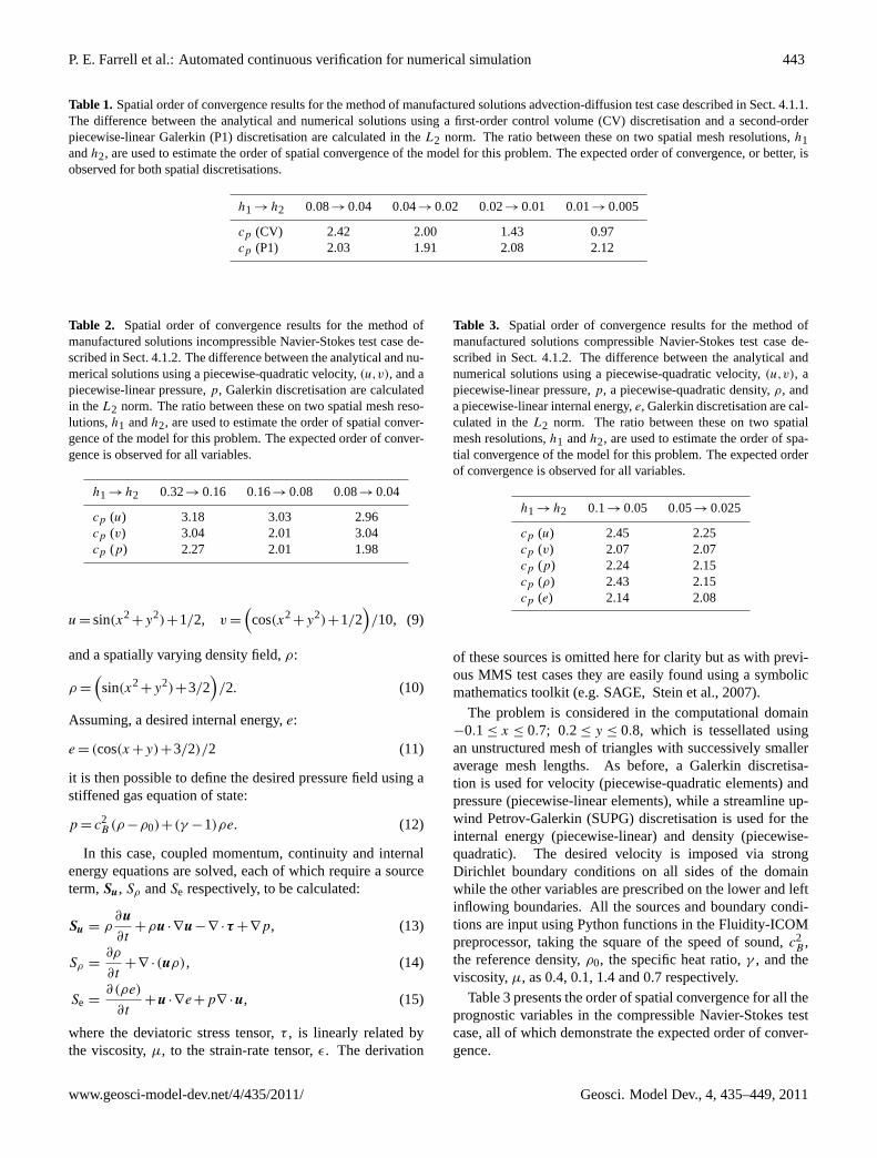
Fig. 4. Left and centre: Numerical approximations tou andp at three resolutions:1x = 1/16 (dotted line), 1/32 (dashed line) and 1/256(solid line). The values fromBotella and Peyret(1998) are plotted as circles. Right: The root-mean-square errors between the numericalsolution and the data fromBotella and Peyret(1998) for u (solid line) andp (dashed line), and the absolute value of the difference betweenthe numerical and benchmark kinetic energy (dotted line) taken fromBruneau and Saad(2006). A line indicating second order convergenceis also shown.

The method of manufactured solutions is an extremely ver-satile code verification tool. As well as increasing the com-plication of the problems considered, as done above, equa-tions may also be simplified. By considering the terms inequation sets individually within an automated testing plat-form any new coding error introduced may be pinpointed al-most instantaneously, even within a large code base. This hasmotivated the development of over forty MMS test cases inthe Fluidity-ICOM verification suite, all of which assert thatthe expected order of convergence is maintained after eachrevision of the code.

4.1.3 The lid-driven cavity

The lid-driven cavity is a problem that is often used as partof the verification procedure for CFD codes. The geometryand boundary conditions are simple to prescribe and in twodimensions there are a number of highly accurate numericalbenchmark solutions available for a wide range of Reynoldsnumbers (Botella and Peyret, 1998; Bruneau and Saad, 2006;Erturk et al., 2005). Here the two-dimensional problem at aReynolds number of 1000 is given as an example.

The unsteady momentum equations with nonlinear advec-tion and viscosity terms are solved in a unit square in thex

andy directions along with the continuity equation, whichenforces incompressibility. No-slip velocity boundary con-ditions are imposed on boundariesx = 0,1 andy = 0, andthe prescribed velocityu = 1, v = 0 are set on the boundaryy = 1 (the “lid”). The problem is initialised with a zero veloc-ity field and the solution allowed to converge to steady statevia time-stepping. A subset of the benchmark data availablefrom the literature is then used to test for numerical conver-gence. Here this involves the calculation of the kinetic energy∫

�

(u2+v2) d�, (16)

which is compared against the value 0.044503 taken fromBruneau and Saad(2006). In addition, thex-component of

velocity and pressure are evaluated at 17 points along theline x = 0.5 and compared against the data fromBotella andPeyret(1998).

Plots of the solutions and benchmark data are given inFig. 4. Also shown is a plot of the error convergence withmesh spacing. A regular triangular mesh is used with pro-gressive uniform refinement in thex,y plane. Second orderspatial convergence can clearly be seen for the three quanti-ties compared.

The automated assertions in this case are that second orderconvergence is attained and that the magnitude of errors inthe three quantities does not increase with code updates.

4.1.4 Flow past a sphere: drag calculation

In this test, uniform flow past an isolated sphere is simulatedand the drag on the sphere is calculated and compared to acurve optimised to fit a large amount of experimental data.

The sphere is of unit diameter centred at the origin. Theentire domain is the cuboid defined by−10≤ x ≤ 20,−10≤

y ≤ 10, −10≤ z ≤ 10. The unsteady momentum equationswith nonlinear advection and viscous terms along with theincompressibility constraint are solved. Free slip velocityboundary conditions are applied at the four lateral bound-aries,u = 1 is applied at the inflow boundaryx = −10, and afree stress boundary condition applied to the outflow atx =

20. A series of Reynolds numbers in the rangeRe ∈ [1,1000]are considered. The problem is run for a long enough pe-riod that the low Reynolds number simulations reach steadystate, and the higher Reynolds number runs long enough thata wake develops behind the sphere and boundary layers onthe sphere are formed. This is deemed sufficient for the pur-poses of this test which is not an in-depth investigation ofthe physics of this problem, nor an investigation of the op-timal set of numerical options to use. Here an unstructuredtetrahedral mesh is used along with an adaptive remeshingalgorithm (Pain et al., 2001). Figure5 shows a snapshot ofthe mesh and velocity vectors taken from a Reynolds number

Geosci. Model Dev., 4, 435–449, 2011 www.geosci-model-dev.net/4/435/2011/

P. E. Farrell et al.: Automated continuous verification for numerical simulation 445

100

102

104

10−1

100

101

102

Reynolds number

CD

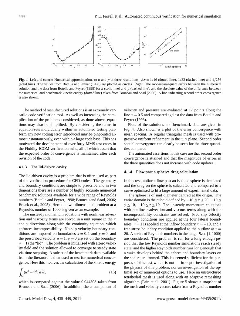
Fig. 5. Left: unstructured adapted mesh from flow past a sphere simulation atRe = 103, with half the domain cut away to display refinementclose to the sphere and in its wake. Centre: a blow up of the mesh and velocity vectors on a plane through the centre of the domain.Right: comparisons between the computed drag coefficient (circles) and the correlation (solid line) given by expression (18) in the rangeRe ∈ [1,1000].

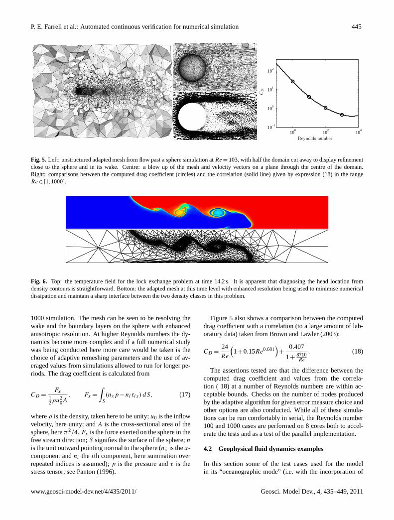
Fig. 6. Top: the temperature field for the lock exchange problem at time 14.2 s. It is apparent that diagnosing the head location fromdensity contours is straightforward. Bottom: the adapted mesh at this time level with enhanced resolution being used to minimise numericaldissipation and maintain a sharp interface between the two density classes in this problem.

1000 simulation. The mesh can be seen to be resolving thewake and the boundary layers on the sphere with enhancedanisotropic resolution. At higher Reynolds numbers the dy-namics become more complex and if a full numerical studywas being conducted here more care would be taken is thechoice of adaptive remeshing parameters and the use of av-eraged values from simulations allowed to run for longer pe-riods. The drag coefficient is calculated from

CD =Fx

12ρu2

0A, Fx =

∫S

(nxp−niτix) dS, (17)

whereρ is the density, taken here to be unity;u0 is the inflowvelocity, here unity; andA is the cross-sectional area of thesphere, hereπ2/4. Fx is the force exerted on the sphere in thefree stream direction;S signifies the surface of the sphere;n

is the unit outward pointing normal to the sphere (nx is thex-component andni the ith component, here summation overrepeated indices is assumed);p is the pressure andτ is thestress tensor; seePanton(1996).

Figure5 also shows a comparison between the computeddrag coefficient with a correlation (to a large amount of lab-oratory data) taken fromBrown and Lawler(2003):

CD =24

Re

(1+0.15Re0.681

)+

0.407

1+8710Re

. (18)

The assertions tested are that the difference between thecomputed drag coefficient and values from the correla-tion ( 18) at a number of Reynolds numbers are within ac-ceptable bounds. Checks on the number of nodes producedby the adaptive algorithm for given error measure choice andother options are also conducted. While all of these simula-tions can be run comfortably in serial, the Reynolds number100 and 1000 cases are performed on 8 cores both to accel-erate the tests and as a test of the parallel implementation.

4.2 Geophysical fluid dynamics examples

In this section some of the test cases used for the modelin its “oceanographic mode” (i.e. with the incorporation of

www.geosci-model-dev.net/4/435/2011/ Geosci. Model Dev., 4, 435–449, 2011

446 P. E. Farrell et al.: Automated continuous verification for numerical simulation

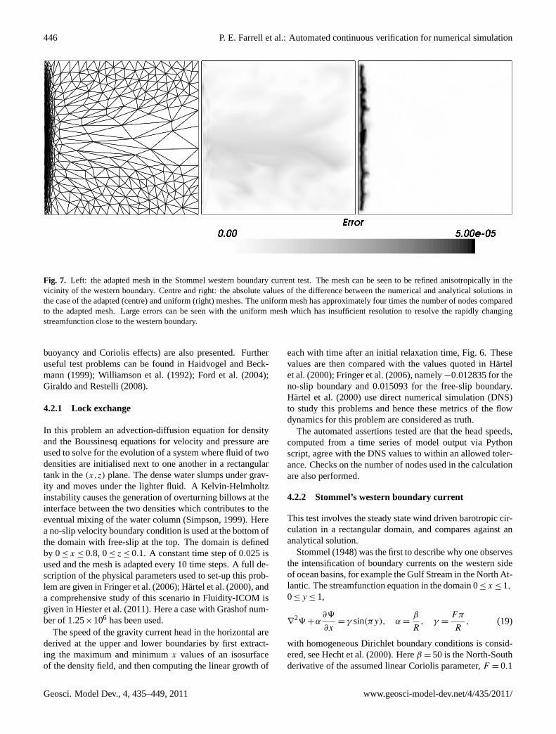
Fig. 7. Left: the adapted mesh in the Stommel western boundary current test. The mesh can be seen to be refined anisotropically in thevicinity of the western boundary. Centre and right: the absolute values of the difference between the numerical and analytical solutions inthe case of the adapted (centre) and uniform (right) meshes. The uniform mesh has approximately four times the number of nodes comparedto the adapted mesh. Large errors can be seen with the uniform mesh which has insufficient resolution to resolve the rapidly changingstreamfunction close to the western boundary.

buoyancy and Coriolis effects) are also presented. Furtheruseful test problems can be found inHaidvogel and Beck-mann(1999); Williamson et al.(1992); Ford et al.(2004);Giraldo and Restelli(2008).

4.2.1 Lock exchange

In this problem an advection-diffusion equation for densityand the Boussinesq equations for velocity and pressure areused to solve for the evolution of a system where fluid of twodensities are initialised next to one another in a rectangulartank in the(x,z) plane. The dense water slumps under grav-ity and moves under the lighter fluid. A Kelvin-Helmholtzinstability causes the generation of overturning billows at theinterface between the two densities which contributes to theeventual mixing of the water column (Simpson, 1999). Herea no-slip velocity boundary condition is used at the bottom ofthe domain with free-slip at the top. The domain is definedby 0≤ x ≤ 0.8, 0≤ z ≤ 0.1. A constant time step of 0.025 isused and the mesh is adapted every 10 time steps. A full de-scription of the physical parameters used to set-up this prob-lem are given inFringer et al.(2006); Hartel et al.(2000), anda comprehensive study of this scenario in Fluidity-ICOM isgiven inHiester et al.(2011). Here a case with Grashof num-ber of 1.25×106 has been used.

The speed of the gravity current head in the horizontal arederived at the upper and lower boundaries by first extract-ing the maximum and minimumx values of an isosurfaceof the density field, and then computing the linear growth of

each with time after an initial relaxation time, Fig.6. Thesevalues are then compared with the values quoted inHartelet al.(2000); Fringer et al.(2006), namely−0.012835 for theno-slip boundary and 0.015093 for the free-slip boundary.Hartel et al.(2000) use direct numerical simulation (DNS)to study this problems and hence these metrics of the flowdynamics for this problem are considered as truth.

The automated assertions tested are that the head speeds,computed from a time series of model output via Pythonscript, agree with the DNS values to within an allowed toler-ance. Checks on the number of nodes used in the calculationare also performed.

4.2.2 Stommel’s western boundary current

This test involves the steady state wind driven barotropic cir-culation in a rectangular domain, and compares against ananalytical solution.

Stommel(1948) was the first to describe why one observesthe intensification of boundary currents on the western sideof ocean basins, for example the Gulf Stream in the North At-lantic. The streamfunction equation in the domain 0≤ x ≤ 1,

0≤ y ≤ 1,

∇29 +α

∂9

∂x= γ sin(πy), α =

β

R, γ =

Fπ

R, (19)

with homogeneous Dirichlet boundary conditions is consid-ered, seeHecht et al.(2000). Hereβ = 50 is the North-Southderivative of the assumed linear Coriolis parameter,F = 0.1

Geosci. Model Dev., 4, 435–449, 2011 www.geosci-model-dev.net/4/435/2011/

P. E. Farrell et al.: Automated continuous verification for numerical simulation 447

is the strength of the wind forcing which takes the formτ = −F cos(πy), andR = 1 is the strength of the assumedlinear frictional force. The analytical solution to (Eq.19) isgiven by

9(x,y) = γ

(1

π

)2

sin(πy)(peAx

+qeBx−1

), (20)

p =1−eB

eA −eB, q = 1−p (21)

A = −α

2+

√α2

4+π2, (22)

B = −α

2−

√α2

4+π2. (23)

Figure7 shows a comparison of results obtained with uni-form and anisotropic adaptive refinement. The form of thestreamfunction yields a velocity field with strong shear in thedirection normal to the western boundary. The error measureand adaptive remeshing algorithms used here yield a meshwhich has long, thin elements aligned with the boundary.The error plots show the high error focused in the westernboundary region in the case of the uniform resolution mesh(Fig. 7).

The automatic assertions here involve ensuring errors fromuniform and adaptive mesh calculations are within accept-able bounds of the analytical solution. In particular, theL2norm of the error obtained with the adapted mesh is checkedto be an order of magnitude lower than that with the fixedmesh, with the adapted mesh using approximately one quar-ter the number of nodes. For further details of this problemsolved using Fluidity-ICOM with isotropic and anisotropicmesh adaptivity seePiggott et al.(2009).

5 Conclusions

Automated continuous testing is widely regarded as industrybest practice in the software engineering community, but thismessage has not yet fully penetrated the numerical modellingcommunity. Rigorous verification is necessary for users tohave confidence in the model results, and is generally a re-quirement for deployment to industry. If the model is underactive development, these processes must run continuouslyas the model is changed; it should therefore be automated.This paper has presented an overview of the software infras-tructure uses to automate the Fluidity-ICOM test suite, aswell as several of the test cases used.

The deployment of the test suite has yielded dramatic im-provements in code quality and programmer efficiency. Al-most no developer time is wasted investigating the failure ofsimulations that used to work. Since feedback about a changeto the code is given almost immediately, any errors intro-duced by new code development can be rapidly fixed. As

the test suite acts to lock in correct behaviour of the compu-tational model, the computational model becomes provablymore efficient and more accurate over time.

As geoscientific simulations become ever more complex,the software complexity of the computational models in-creases with it; therefore, the standard of software engineer-ing used to write and manage those scientific models mustrise also. The widespread deployment of automated frame-works such as that described here is a necessary step if soci-ety at large is to trust the results of geoscientific models.

Acknowledgements.The authors would like to thank J. R. Maddi-son and H. R. Hiester for helpful discussions and input to the workpresented here. The authors wish to acknowledge support from theUK Natural Environment Research Council (grants NE/C52101X/1and NE/C51829X/1) and support from the Imperial College HighPerformance Computing Service, the Grantham Institute forClimate Change, and the Institute of Shock Physics.

Edited by: R. Redler

References

Adrion, W. R., Branstad, M. A., and Cherniavsky, J. C.: Validation,Verification, and Testing of Computer Software, ACM Comput-ing Surveys, 14, 159–192,doi:10.1145/356876.356879, 1982.

Babuska, I. and Oden, J. T.: Verification and validation in computa-tional engineering and science: basic concepts, Comput. MethodAppl. M., 193, 4057–4066,doi:10.1016/j.cma.2004.03.002,2004.

Botella, O. and Peyret, R.: Benchmark spectral results on the lid-driven cavity flow, Comput. Fluids, 27, 421–433, 1998.

Brown, P. P. and Lawler, D. F.: Sphere Drag and SettlingVelocity Revisited, J. Environ. Eng.-ASCE, 129, 222–231,doi:10.1061/(ASCE)0733-9372(2003)129:3(222), 2003.

Bruneau, C. H. and Saad, M.: The 2D lid-driven cavity problemrevisited, Comput. Fluids, 35, 326–348, 2006.

Collins-Sussman, B., Fitzpatrick, B. W., and Pilato, C. M.: VersionControl with Subversion, O’Reilly & Associates, available at:http://subversion.apache.org, last access: 16 May 2011, 2004.

Davies, T., Cullen, M. J. P., Malcolm, A. J., Mawson, M. H.,Staniforth, A., White, A. A., and Wood, N.: A new dynami-cal core for the Met Office’s global and regional modelling ofthe atmosphere, Q. J. Roy. Meteorol. Soc., 131, 1759–1782,doi:10.1256/qj.04.101, 2005.

Deleersnijder, E., Fichefet, T., Hanert, E., Legat, V., Remacle, J.-F.,and Frazao, S. S.: Taking up the challenges of multi-scale ma-rine modelling, available at:http://sites-final.uclouvain.be/slim/assets/files/documents/ProposalWeb2.pdf, excerpts from a pro-posal for a Concerted Research Actions (ARC) programme, lastaccess: 16 May 2011, 2010.

Easterbrook, S. M. and Johns, T. C.: Engineering the Software forUnderstanding Climate Change, Comput. Sci. Eng., 11, 65–74,doi:10.1109/MCSE.2009.193, 2009.

Erturk, E., Corke, T. C., and Gokcol, C.: Numerical solutions of 2-D steady incompressible driven cavity ow at high Reynolds num-bers, Int. J. Numer. Meth. Fl., 48, 747–774,doi:10.1002/fld.953,2005.

www.geosci-model-dev.net/4/435/2011/ Geosci. Model Dev., 4, 435–449, 2011

448 P. E. Farrell et al.: Automated continuous verification for numerical simulation

Ford, R., Pain, C. C., Piggott, M. D., Goddard, A. J. H., de Oliveira,C. R. E., and Umpleby, A. P.: A Nonhydrostatic Finite-ElementModel for Three-Dimensional Stratified Oceanic Flows, Part II:Model Validation, Month. Weather Rev., 132, 2832–2844, 2004.

Fringer, O. B., Gerritsen, M., and Street, R. L.: An unstructured-grid, finite-volume, nonhydrostatic, parallel coastal ocean simu-lator, Ocean Model., 14, 139–173, 2006.

Giraldo, F. X. and Restelli, M.: A study of spectral element anddiscontinuous Galerkin methods for the Navier-Stokes equa-tions in nonhydrostatic mesoscale atmospheric modeling: Equa-tion sets and test cases, J. Comput. Phys., 227, 3849–3877,doi:10.1016/j.jcp.2007.12.009, 2008.

Graham, S. L., Kessler, P. B., and McKusick, M. K.: gprof: a CallGraph Execution Profiler, in: SIGPLAN Symposium on Com-piler Construction, 120–126,doi:10.1145/872726.806987, 1982.

Griffies, S. M.: Elements of MOM4p1, available at:http://data1.gfdl.noaa.gov/∼arl/pubrel/r/mom4p1/src/mom4p1/doc/guide4p1.pdf, last access: 16 May 2011, 2009.

Griffies, S. M., Harrison, M. J., Pacanowski, R. C., and Rosati,A.: A Technical guide to MOM4, available at:http://data1.gfdl.noaa.gov/∼arl/pubrel/o/old/doc/mom4p0guide.pdf, last access:16 May 2011, 2004.

Haidvogel, D. B. and Beckmann, A.: Numerical Ocean CirculationModeling, Imperial College Press, River Edge, NJ, USA, 1999.

Ham, D. A., Farrell, P. E., Gorman, G. J., Maddison, J. R., Wilson,C. R., Kramer, S. C., Shipton, J., Collins, G. S., Cotter, C. J., andPiggott, M. D.: Spud 1.0: generalising and automating the userinterfaces of scientific computer models, Geosci. Model Dev., 2,33–42,doi:10.5194/gmd-2-33-2009, 2009.

Hartel, C., Meiburg, E., and Necker, F.: Analysis and direct numer-ical simulation of the flow at a gravity-current head, Part I, Flowtopology and front speed for slip and no-slip boundaries, J. FluidMech., 418, 189–212, 2000.

Hecht, M. W., Wingate, B. A., and Kassis, P.: A better, morediscriminating test problem for ocean tracer transport, OceanModel., 2, 1–15, 2000.

Hiester, H. R., Piggott, M. D., and Allison, P. A.: The im-pact of mesh adaptivity on the gravity current front speedin a 2D lock-exchange, Ocean Model., 38, 1–2 , 1–21,doi:10.1016/j.ocemod.2011.01.003, 2011

Howden, W. E.: Reliability of the Path Analysis Testing Strategy,IEEE T. Software Eng., SE-2, 208–215, 1976.

Jones, E., Oliphant, T., Peterson, P., et al.: SciPy: Open source sci-entific tools for Python, available at:http://www.scipy.org, lastaccess: 16 May 2011, 2001.

Knupp, P., Ober, C. C., and Bond, R. B.: Measuring progressin order-verification within software development projects, Eng.Comput., 23, 271–282,doi:10.1007/s00366-007-0066-x, 2007.

Madec, G., Delecluse, P., and Imbard, M.: OPA 8.1 ocean generalcirculation model reference manual, Paris VI, France, note 11,1998.

Marshall, J., Adcroft, A., Hill, C., Perelman, L., and Heisey, C.:A finite-volume, incompressible Navier Stokes model for studiesof the ocean on parallel computers, J. Geophys. Res., 102, 5753–5766,doi:10.1029/96JC02775, 1997.

NEMO Consortium: The Nemo Consortium Agreement, availabeat: http://www.nemo-ocean.eu/, last access: 16 May 2011, 2008.

Oberkampf, W. L. and Atrucano, T. G.: Verification and Valida-tion in Computational Fluid Dynamics, Tech. Rep. SAND 2002-

0529, Sandia National Laboratories, Albuquerque, NM, 2002.Oberkampf, W. L., Sindir, M. M., and Conlisk, A. T.: Guide for

the Verification and Validation of Computational Fluid DynamicsSimulations, Tech. Rep. G-077-98, American Institute of Aero-nautics and Astronautics, 1998.

Oreskes, N., Shrader-Frechette, K., and Belitz, K.: Ver-ification, Validation, and Confirmation of NumericalModels in the Earth Sciences, Science, 263, 641–646,doi:10.1126/science.263.5147.641, 1994.

Pain, C. C., Umpleby, A. P., de Oliveira, C. R. E., and Goddard, A.J. H.: Tetrahedral mesh optimisation and adaptivity for steady-state and transient finite element calculations, Comput. MethodAppl. M., 190, 3771–3796,doi:10.1016/S0045-7825(00)00294-2, 2001.

Pain, C. C., Piggott, M. D., Goddard, A. J. H., Fang, F., Gorman,G. J., Marshall, D. P., Eaton, M. D., Power, P. W., and de Oliveira,C. R. E.: Three-dimensional unstructured mesh ocean modelling,Ocean Model., 10, 5–33,doi:10.1016/j.ocemod.2004.07.005,2005.

Panton, R. L.: Incompressible Flow, Wiley-Interscience, 1996.Piggott, M. D., Gorman, G. J., Pain, C. C., Allison, P. A., Candy,

A. S., Martin, B. T., and Wells, M. R.: A new computationalframework for multi-scale ocean modelling based on adaptingunstructured meshes, Int. J. Numer. Meth. Fl., 56, 1003–1015,doi:10.1002/fld.1663, 2008.

Piggott, M. D., Farrell, P. E., Wilson, C. R., Gorman, G. J.,and Pain, C. C.: Anisotropic mesh adaptivity for multi-scaleocean modelling, Philos. T. Roy. Soc. A, 367, 4591–4611,doi:10.1098/rsta.2009.0155, 2009.

Popper, K. R.: The Logic of Scientific Discovery, Routledge, Lon-don, 1959.

Roache, P. J.: Code Verification by the Method of Man-ufactured Solutions, J. Fluid. Eng. T. ASME, 124, 4–10,doi:10.1115/1.1436090, 2002.

Salari, K. and Knupp, P.: Code Verification by the Method of Man-ufactured Solutions, Tech. Rep. SAND2000-1444, Sandia Na-tional Laboratories, Albuquerque, NM, 2000.

Schroeder, W., Martin, K., and Lorensen, B.: The VisualizationToolkit: An Object-Oriented Approach to 3D Graphics, KitWare,Inc., 4th Edn., available at:http://www.vtk.org, last access: 16May 2011, 2006.

Simpson, J. E.: Gravity Currents in the Environment and the Labo-ratory, Cambridge University Press, 2nd Edn., 1999.

Song, Y. and Haidvogel, D. B.: A Semi-implicit Ocean Circu-lation Model Using a Generalized Topography-FollowingCoordinate System, J. Comput. Phys., 115, 228–244,doi:10.1006/jcph.1994.1189, 1994.

Stein, W., Abbott, T., Abshoff, M., et al.: SAGE Mathematics Soft-ware, The SAGE Group, available at:http://www.sagemath.org,last access: 16 May 2011, 2007.

Stern, F., Wilson, R. V., Coleman, H. W., and Paterson, E. G.: Com-prehensive approach to verification and validation of CFD simu-lations, 1: Methodology and procedures, J. Fluid. Eng. T. ASME,123, 793–802, 2001.

Stommel, H.: The westward intensification of wind-driven oceancurrents, Transactions of the American Geophysical Union, 29,202–206, 1948.

Trefethen, L. N.: Numerical Analysis, in: Princeton Companion toMathematics, edited by: Gowers, T., Princeton University Press,

Geosci. Model Dev., 4, 435–449, 2011 www.geosci-model-dev.net/4/435/2011/

P. E. Farrell et al.: Automated continuous verification for numerical simulation 449

section IV. 21, 604–615, 2008.White, L., Deleersnijder, E., and Legat, V.: A three-

dimensional unstructured mesh finite element shallow-watermodel, with application to the flows around an island andin a wind-driven, elongated basin, Ocean Model., 22, 26–47,doi:10.1016/j.ocemod.2008.01.001, 2008.

Williamson, D. L., Drake, J., Hack, J., Akob, R., and Swartzrauber,P. N.: A standard test set for numerical approximations to theshallow water equations in spherical geometry, J. Comput. Phys.,102, 211–224, 1992.

www.geosci-model-dev.net/4/435/2011/ Geosci. Model Dev., 4, 435–449, 2011