gloptipoly 3 - a matlab package for globally minimizing
TRANSCRIPT

GloptiPoly 3 -A Matlab package for
globally minimizing polynomial moments
Didier HENRION1,2
Jean-Bernard LASSERRE1
Johan LOFBERG3
1LAAS-CNRS Toulouse, FR2Czech Tech Univ Prague, CZ
3ETH Zurich, CH
Univ Waterloo May 2004

Towards GloptiPoly 3 -A future Matlab package for
globally minimizing polynomial moments
Didier HENRION1,2
Jean-Bernard LASSERRE1
Johan LOFBERG3
1LAAS-CNRS Toulouse, FR2Czech Tech Univ Prague, CZ
3ETH Zurich, CH
Univ Waterloo May 2004
Outline
1. Brief description of GloptiPoly
2. From version 2 to version 3
3. Some case studies:
• Comparative performances of SDP solvers
• Moment substitutions
• Motzkin polynomial
4. Some research directions

Part 1
Brief description
of GloptiPoly

Brief description
GloptiPoly is as an open-source, general
purpose and user-friendly Matlab software
Aimed at small to medium non-convex global
optimization problems with multivariable real-
valued polynomial objective functions and
constraints
Software and documentation available at
www.laas.fr/∼henrion/software/gloptipoly
Version 2 described in ACM TOMS June 2003

Metholodogy
GloptiPoly builds and solves a hierarchy of suc-
cessive convex linear matrix inequality (LMI)
relaxations of increasing size, whose optima are
guaranteed to converge asymptotically to the
global optimum
Relaxations are built from LMI formulation of
• primal sum of squares (SOS) decomposition
• dual theory of moments
of positive multivariable polynomials
In practice convergence is ensured fast
typically at 2nd or 3rd LMI relaxation

LMI relaxation technique
Polynomial optimization problem
min g0(x)s.t. gk(x) ≥ 0, k = 1, . . . ,m
When p? is the global optimum, SOS
representation of positive polynomial
g0(x)− p? = q0(x) +∑mk=1 gk(x)qk(x)
where unknowns qk(x) are SOS polynomials
similar to Karush/Kuhn/Tucker multipliers
Using LMI representation of SOS polynomials
successive LMI relaxations are obtained by in-
creasing degrees of sought polynomials qk(x)
Theoretical proof of asymptotic convergence...
..but no tight degree upper bounds (not yet)

LMI relaxations: illustration (1)
Non-convex quadratic problem
max x2s.t. 3− 2x2 − x1
2 − x22 ≥ 0
−x1 − x2 − x1x2 ≥ 01 + x1x2 ≥ 0
Non-convex feasible set delimited by circularand hyperbolic arcs
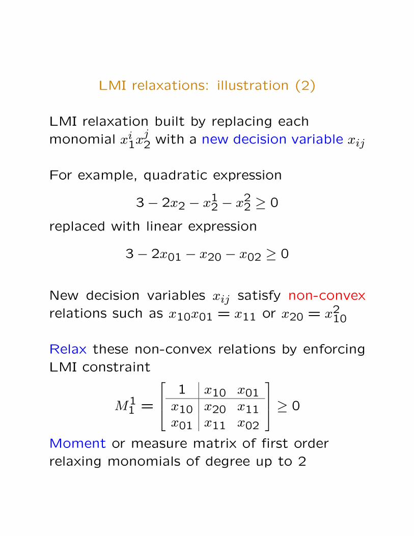
LMI relaxations: illustration (2)
LMI relaxation built by replacing each
monomial xi1xj2 with a new decision variable xij
For example, quadratic expression
3− 2x2 − x12 − x
22 ≥ 0
replaced with linear expression
3− 2x01 − x20 − x02 ≥ 0
New decision variables xij satisfy non-convex
relations such as x10x01 = x11 or x20 = x210
Relax these non-convex relations by enforcing
LMI constraint
M11 =
1 x10 x01x10 x20 x11x01 x11 x02
≥ 0
Moment or measure matrix of first order
relaxing monomials of degree up to 2

LMI relaxations: illustration (3)
First LMI relaxation given by
max x01
s.t.
1 x10 x01
x10 x20 x11
x01 x11 x02
� 0
3− 2x01 − x20 − x02 ≥ 0−x10 − x01 − x11 ≥ 01 + x11 ≥ 0
Projection of the LMI feasible set onto the plane x10, x01of first-order moments
LMI optimum = 2 = upper-bound on global optimum
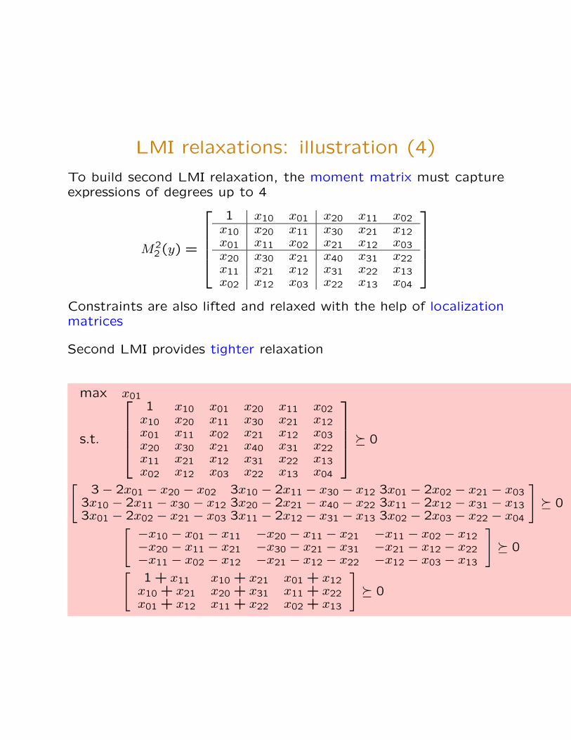
LMI relaxations: illustration (4)
To build second LMI relaxation, the moment matrix must captureexpressions of degrees up to 4
M22 (y) =
1 x10 x01 x20 x11 x02x10 x20 x11 x30 x21 x12x01 x11 x02 x21 x12 x03x20 x30 x21 x40 x31 x22x11 x21 x12 x31 x22 x13x02 x12 x03 x22 x13 x04
Constraints are also lifted and relaxed with the help of localizationmatrices
Second LMI provides tighter relaxation
max x01
s.t.
1 x10 x01 x20 x11 x02x10 x20 x11 x30 x21 x12x01 x11 x02 x21 x12 x03x20 x30 x21 x40 x31 x22x11 x21 x12 x31 x22 x13x02 x12 x03 x22 x13 x04
� 0
[3− 2x01 − x20 − x02 3x10 − 2x11 − x30 − x12 3x01 − 2x02 − x21 − x03
3x10 − 2x11 − x30 − x12 3x20 − 2x21 − x40 − x22 3x11 − 2x12 − x31 − x133x01 − 2x02 − x21 − x03 3x11 − 2x12 − x31 − x13 3x02 − 2x03 − x22 − x04
]� 0[ −x10 − x01 − x11 −x20 − x11 − x21 −x11 − x02 − x12
−x20 − x11 − x21 −x30 − x21 − x31 −x21 − x12 − x22−x11 − x02 − x12 −x21 − x12 − x22 −x12 − x03 − x13
]� 0[
1 + x11 x10 + x21 x01 + x12x10 + x21 x20 + x31 x11 + x22x01 + x12 x11 + x22 x02 + x13
]� 0

LMI relaxations: illustration (5)
Optimal value of 2nd LMI relaxation = 1.6180
= global optimum within numerical accuracy
Numerical certificate = moment matrix has
rank one
First order moments (x∗10, x∗01) = (−0.6180,1.6180)
provides optimal solution of original problem

Part 2
From version 2
to version 3
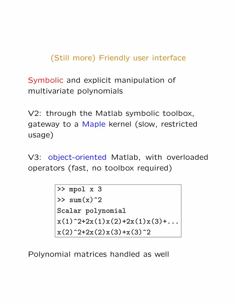
(Still more) Friendly user interface
Symbolic and explicit manipulation of
multivariate polynomials
V2: through the Matlab symbolic toolbox,
gateway to a Maple kernel (slow, restricted
usage)
V3: object-oriented Matlab, with overloaded
operators (fast, no toolbox required)
>> mpol x 3
>> sum(x)^2
Scalar polynomial
x(1)^2+2x(1)x(2)+2x(1)x(3)+...
x(2)^2+2x(2)x(3)+x(3)^2
Polynomial matrices handled as well

Theory of moments
Polynomial global optimization
minx g0(x)s.t. x ∈ K = {x ∈ Rn : gi(x) ≥ 0, i = 1,2, . . .}
on a semialgebraic set K ⊂ Rn
Defining µ as a probability measure
the equivalent moment problem is
minµ
∫g0(x)µ(dx)
s.t. µ(K) = 1
meaning that µ is supported on K, implying
that µ(Rn/K) = 0
Measure support constraints are then relaxed
with moment constraints∫f2(x)gi(x)µ(dx) ≥ 0 ∀f
⇒ LMI if the degree of polynomial f is bounded

More moment problems
Ex. rational optimization problem (de Klerk,Jibetean)
minx
p(x)
q(x)s.t. x ∈ K
becomes the moment problem
minµ
∫p(x)µ(dx)
s.t. µ(Rn/K) = 0∫q(x)µ(dx) = 1
with an additional moment constraint(q(x) ≡ 1 ⇒ µ is a probability measure, seeprevious problem)
Robust SDP problems also become momentproblems with additional linear momentconstraints
Problems with several measures µ1, µ2.. arisein performance analysis in mathematical finance
Cf previous talk..

Manipulating moments
In summary, a measure µ corresponds toa vector of variables x ∈ Rn with moments
∫xαµ(dx)
Associated with semialgebraic (polynomial)constraints x ∈ K = {x ∈ Rn : g(x) ≥ 0} aresupport constraints
µ(Rn/K) = 0
Finally, there may be additional linear momentconstraints
∫h(x)µ(dx) ≥ 0
In a Matlab setting, depending on the context,we use the same symbol to denote the mono-mial xα and its associated moment
∫xαdµ
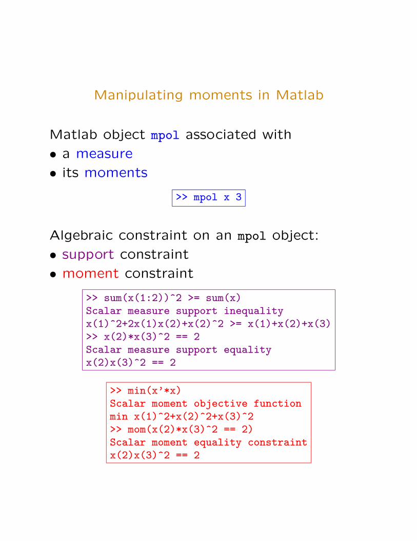
Manipulating moments in Matlab
Matlab object mpol associated with
• a measure
• its moments
>> mpol x 3
Algebraic constraint on an mpol object:
• support constraint
• moment constraint
>> sum(x(1:2))^2 >= sum(x)Scalar measure support inequalityx(1)^2+2x(1)x(2)+x(2)^2 >= x(1)+x(2)+x(3)>> x(2)*x(3)^2 == 2Scalar measure support equalityx(2)x(3)^2 == 2
>> min(x’*x)Scalar moment objective functionmin x(1)^2+x(2)^2+x(3)^2>> mom(x(2)*x(3)^2 == 2)Scalar moment equality constraintx(2)x(3)^2 == 2

Calling sequence
mdef: moment problem definition
msol: solve moment problem
Example: radius of 3 intersecting ellipses
max x21 + x2
2s.t. 2x2
1 + 3x22 + 2x1x2 ≤ 1
3x21 + 2x2
2 − 4x1x2 ≤ 1x2
1 + 6x22 − 4x1x2 ≤ 1
>> mpol x 2>> LMI = 2; % LMI relaxation order>> radius = x(1)^2+x(2)^2;>> P = mdef(max(radius),...
2*x(1)^2+3*x(2)^2+2*x(1)*x(2)<=1,...3*x(1)^2+2*x(2)^2-4*x(1)*x(2)<=1,...x(1)^2+6*x(2)^2-4*x(1)*x(2)<=1,...LMI);
>> x = msol(P);>> x1=x{1}’,x2=x{2}’x1 =
-0.6450 -0.1047x2 =
0.6450 0.1047>> double(radius)ans =
0.4270

Using SDP solvers
V2: Exclusive use of Jos Sturm’s SeDuMi solver
V3: Solver-independent thanks to Johan Lofberg’s
YALMIP parser
So far we have been using (more or less)
successfully
• CSDP 4.5 (Borchers)
• DSDP 4.5 (Benson/Ye)
• SDPT3 3.1 (Toh/Todd/Tutuncu)
• SDPA 6.0 through SDPAM 2.0 (Kojima)
• SeDuMi 1.05 (Sturm)
• LMILAB R13 (Gahinet/Nemirovskii)
• PENSDP 1.1 (Kocvara/Stingl)
>> P = mdef(..);
>> mset(’solver’,’sdpt3’);
>> x = msol(P);

Part 3
Some case studies

Part 3.1
Comparative performance of
SDP solvers

Comparative performances
of SDP solvers
Primal/dual LP in self-dual cone K:
min c?xs.t. Ax = b
x ∈ K
max b?ys.t. c−A?y ∈ K
where x ∈ Rp and y ∈ Rd
We used default tunings of solvers interfaced
with YALMIP 3.0
CPU times on SunBlade 150 workstation with
Matlab R13 under Solaris Unix
Numerical certificate of globality (rank checks)
and extraction algorithm from GloptiPoly V2
Continuous QP optimization problems from
Floudas & Pardalos 1999

QP benchmark problems
FP 2.2: 5v11i2d - LMI3 d461p7987• SeDuMi 24s, CSDP 36s, SDPA 44s, SDPT3 49s• PENSDP 2mn27s• DSDP 4mn32s fails
FP 2.3: 6v11i2d - LMI2 d209p1421• SeDuMi 5.0s, CSDP 7.2s, SDPA 7.8s, PENSDP 8.0s• SDPT3 15s• DSDP 23s fails
FP 2.4: 13v35i2d - LMI2 d2379p17885• SDPT3 7mn19s, CSDP 9mn56s• SeDuMI 42mn30s, SDPA 42mn30s• PENSDP 42mn25s fails• DSDP >1h fails
FP 2.5: 6v15i2d - LMI2 d209p1519• SeDuMi 3.7s• SDPA 7.9s, CSDP 8.0s, SDPT3 11s, DSDP 12s• PENSDP 18s
FP 2.6: 10v31i2d - LMI2 d1000p8107• SDPT3 1mn19s• CSDP 2mn28s, SeDuMi 2mn41s• SDPA 6mn03s, PENSDP 7mn27s• DSDP 7mn03s fails

FP 2.7: 10v25i2d - LMI2 d1000p7381• SDPT3 1mn19s, CSDP 1mn37s• SeDuMi 3mn24s• PENSDP 4mn47s, SDPA 5mn13s• DSDP 5mn40s fails
FP 2.11: 10v10i1e2d - LMI2 d1000p5632• SDPT3 55s• CSDP 1mn21s, SeDuMi 1mn52s• SDPA 3mn03s, PENSDP 3mn47s• DSDP 20mn10s fails
FP 3.3: 10v16i2d - LMI2 d125p1017• SeDuMi 3s• SDPT3 16s• SDPA 0.74s, DSDP 2.1s, CSDP 6.9s, PENSDP 46sall fail (!)
FP 3.4: 6v16i2d - LMI2 d209p1568• SeDuMi 3.9s, CSDP 5.4s• SDPA 7.8s, SDPA 13s, PENSDP 18s• DSDP 24s fails
FP 3.5: 3v8i2d - LMI4 d164p4425• SeDuMi 6.0s, SDPA 6.9s• CSDP 11s• PENSDP 24s, SDPT3 27s• DSDP 45s fails
Problems FP 2.8, FP 2.9, FP 2.11 feature 20 or 24variables and could not be solved without swapping
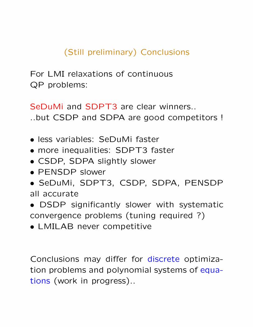
(Still preliminary) Conclusions
For LMI relaxations of continuousQP problems:
SeDuMi and SDPT3 are clear winners....but CSDP and SDPA are good competitors !
• less variables: SeDuMi faster• more inequalities: SDPT3 faster• CSDP, SDPA slightly slower• PENSDP slower• SeDuMi, SDPT3, CSDP, SDPA, PENSDPall accurate• DSDP significantly slower with systematicconvergence problems (tuning required ?)• LMILAB never competitive
Conclusions may differ for discrete optimiza-tion problems and polynomial systems of equa-tions (work in progress)..
Part 3.2
Moment subsitutions

Detecting global optimality
and extracting solutions
Rank condition on moment matrices
ensures global optimality
Solutions extracted by extracting Cholesky
factor of moment matrix, and then solving an
eigenvalue problem
Example: quadratic problem
p∗ = maxx (x1 − 1)2 + (x1 − x2)2 + (x2 − 3)2
s.t. (x1 − 1)2 ≤ 1(x1 − x2)2 ≤ 1(x2 − 3)2 ≤ 1
First LMI relaxation yields p?1 = 3 and rank M1 = 3,extraction algorithm fails due to incomplete monomialbasis
Second LMI relaxation yields p?2 = 2 and
rankM1 = rankM2 = 3
so rank condition ensures global optimality

Cholesky factorization
Moment matrix of order 2 reads
M2 =
1.0000 1.5868 2.2477 2.7603 3.6690 5.23871.5868 2.7603 3.6690 5.1073 6.5115 8.82452.2477 3.6690 5.2387 6.5115 8.8245 12.70722.7603 5.1073 6.5115 9.8013 12.1965 15.99603.6690 6.5115 8.8245 12.1965 15.9960 22.10845.2387 8.8245 12.7072 15.9960 22.1084 32.1036
Positive semidefinite with rank 3
Cholesky factor
V =
−0.9384 −0.0247 0.3447−1.6188 0.3036 0.2182−2.2486 −0.1822 0.3864−2.9796 0.9603 −0.0348−3.9813 0.3417 −0.1697−5.6128 −0.7627 −0.1365
satisfies
M2 = V V ′

Column echelon form
Gaussian elimination on V yields
U =
1 0 00 1 00 0 1−2 3 0−4 2 2−6 0 5
1x1x2x2
1x1x2x2
21 x1 x2
which means that solutions to be extracted
satisfy the system of polynomial equations
x21 = −2 + 3x1
x1x2 = −4 + 2x1 + 2x2x2
2 = −6 + 5x2
in polynomial basis 1, x1, x2
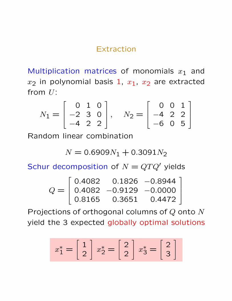
Extraction
Multiplication matrices of monomials x1 and
x2 in polynomial basis 1, x1, x2 are extracted
from U :
N1 =
0 1 0−2 3 0−4 2 2
, N2 =
0 0 1−4 2 2−6 0 5
Random linear combination
N = 0.6909N1 + 0.3091N2
Schur decomposition of N = QTQ′ yields
Q =
0.4082 0.1826 −0.89440.4082 −0.9129 −0.00000.8165 0.3651 0.4472
Projections of orthogonal columns of Q onto N
yield the 3 expected globally optimal solutions
x∗1 =
[12
]x∗2 =
[22
]x∗3 =
[23
]

Moment subsitutions
Moments may satisfy explicit equality constraints
such as x20 = 1, x02 = 1, x30 = x10 etc for
combinatorial problems x2i = 1
Moment constraints may also arise from the
extraction algorithm, when the polynomial
basis is incomplete and some multiplication
matrices are not available
Removing these equality constraints
• significantly reduce the number of variables
• may destroy sparsity
Should we remove these moment constraints
by solving an LSE ?
Should we keep them explicit and forward them
to the SDP solver ?

Substituting moments (1)
Combinatorial quadratic problem
min cTx+ xTQxs.t. −1 ≤ x1x2 + x3x4 ≤ 1
−3 ≤ x1 + x2 + x3 + x4 ≤ 2x2i = 1
Size of LMI relaxations
LMI order m/n non reduced m/n reduced1 14/18 10/102 69/236 15/363 209/1896 15/964 494/10011 15/2115 1000/39607 15/407
Significant reduction
Trivial example since here the maximum
number of moments is 24 − 1 = 15
xα11 x
α22 x
α33 x
α44 with αi = 0/1
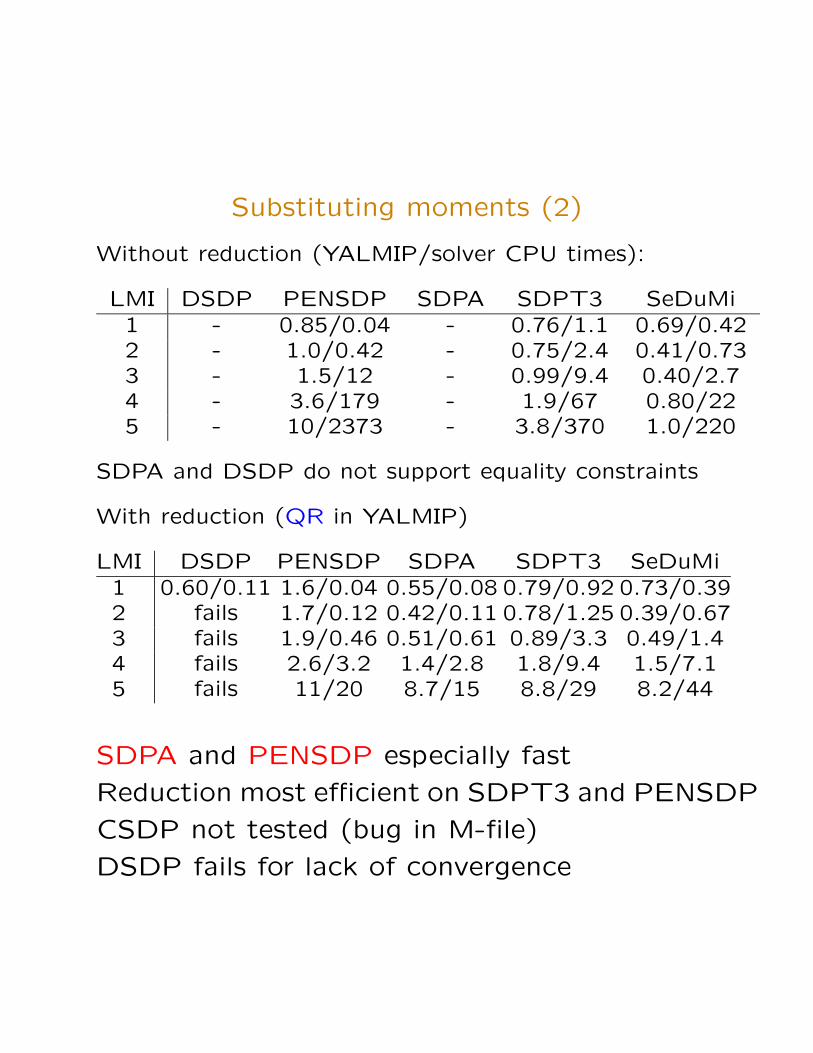
Substituting moments (2)
Without reduction (YALMIP/solver CPU times):
LMI DSDP PENSDP SDPA SDPT3 SeDuMi1 - 0.85/0.04 - 0.76/1.1 0.69/0.422 - 1.0/0.42 - 0.75/2.4 0.41/0.733 - 1.5/12 - 0.99/9.4 0.40/2.74 - 3.6/179 - 1.9/67 0.80/225 - 10/2373 - 3.8/370 1.0/220
SDPA and DSDP do not support equality constraints
With reduction (QR in YALMIP)
LMI DSDP PENSDP SDPA SDPT3 SeDuMi1 0.60/0.11 1.6/0.04 0.55/0.08 0.79/0.92 0.73/0.392 fails 1.7/0.12 0.42/0.11 0.78/1.25 0.39/0.673 fails 1.9/0.46 0.51/0.61 0.89/3.3 0.49/1.44 fails 2.6/3.2 1.4/2.8 1.8/9.4 1.5/7.15 fails 11/20 8.7/15 8.8/29 8.2/44
SDPA and PENSDP especially fast
Reduction most efficient on SDPT3 and PENSDP
CSDP not tested (bug in M-file)
DSDP fails for lack of convergence

Part 3.3
Motzkin polynomial

Motzkin-like polynomial
Polynomial
1
27+ x2y2(x2 + y2 − 1)
vanishes at |x| = |y| =√
3/3 and
remains globally non-negative for real x and y
but cannot be written as an SOS

Minimizing Motzkin polynomial with
GloptiPoly
>> mpol x y
>> motzkin = 1/27+x^2*y^2*(x^2+y^2-1);
>> mset(’solver’,’sedumi’);
>> P = mdef(min(motzkin),3); msol(P);
>> P = mdef(min(motzkin),4); msol(P);
...
For different SDP solvers and LMI orders
we compared
• CPU times
• norms of moment vector
• lower bounds on global optimum

SDP solvers performance
on Motzkin polynomial (1)
CPU times for different LMI orders and
different SDP solvers
DSDP & PENSDP slower for larger problems
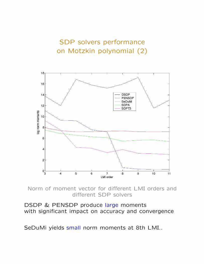
SDP solvers performanceon Motzkin polynomial (2)
Norm of moment vector for different LMI orders anddifferent SDP solvers
DSDP & PENSDP produce large momentswith significant impact on accuracy and convergence
SeDuMi yields small norm moments at 8th LMI..

SDP solvers performanceon Motzkin polynomial (3)
Objective values for different LMI orders anddifferent SDP solvers
Most of the solvers converge numerically to thezero global minimum at the 8th LMI relaxation

Some kind of magic in GloptiPoly
GloptiPoly finds approximate SOSdecomposition of Motzkin polynomial
At 8th LMI relaxation we obtain with SeDuMi
1
27+ x2y2(x2 + y2 − 1) =
32∑i=1
a2i q
2i (x, y) + εr(x, y)
where ‖qi‖2 = ‖r‖2 = 1and ε ≤ 10−8 < a2
i , deg qi ≤ 8
Cone of SOS polynomials is dense in set ofpolynomials nonnegative over box [-1,1]
Numerical inaccuracyhelps finding higher degree
SOS polynomial closeto Motzkin polynomial
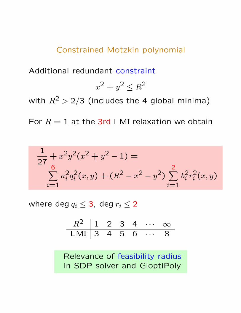
Constrained Motzkin polynomial
Additional redundant constraint
x2 + y2 ≤ R2
with R2 > 2/3 (includes the 4 global minima)
For R = 1 at the 3rd LMI relaxation we obtain
1
27+ x2y2(x2 + y2 − 1) =
6∑i=1
a2i q
2i (x, y) + (R2 − x2 − y2)
2∑i=1
b2i r2i (x, y)
where deg qi ≤ 3, deg ri ≤ 2
R2 1 2 3 4 · · · ∞LMI 3 4 5 6 · · · 8
Relevance of feasibility radiusin SDP solver and GloptiPoly
Part 4
Some research directions

Numerical analysis for polynomials
So far most of the research efforts in numericalanalysis dedicated to real or complex valuedmatrices (Wilkinson)
Numerical conditioning of polynomial bases -alternative choices (Chebyshev, Bernstein..)
A posteriori analysis (Stetter)
Pseudozeros of polynomials (Toh & Trefethen)

Dedicated SDP methods
Structure of moment matrices ?
Univariate = Hankel moment matrix
Multivariate = sparse matrix coeffs
1 x10 x01 x20 x11 x02x10 x20 x11 x30 x21 x12x01 x11 x02 x21 x12 x03x20 x30 x21 x40 x31 x22x11 x21 x12 x31 x22 x13x02 x12 x03 x22 x13 x04
Known sparsity pattern: LMI matrix coeffs inpre-factored form (Cholesky)
Efficient low-rank algebra to compute gradient& Hessian in interior-point codes ?
Moment substitutions: trade-off betweensparsity and number of variables