global scenarios for lac - world...

11

How Nasty will the External Environment Get?Global Scenarios for LAC

RTM Retreat

Washington, DC2 November 2011

Chief Economist OfficeLatin America and the CaribbeanThe World Bank

Rising Global Uncertainty and Risks

2

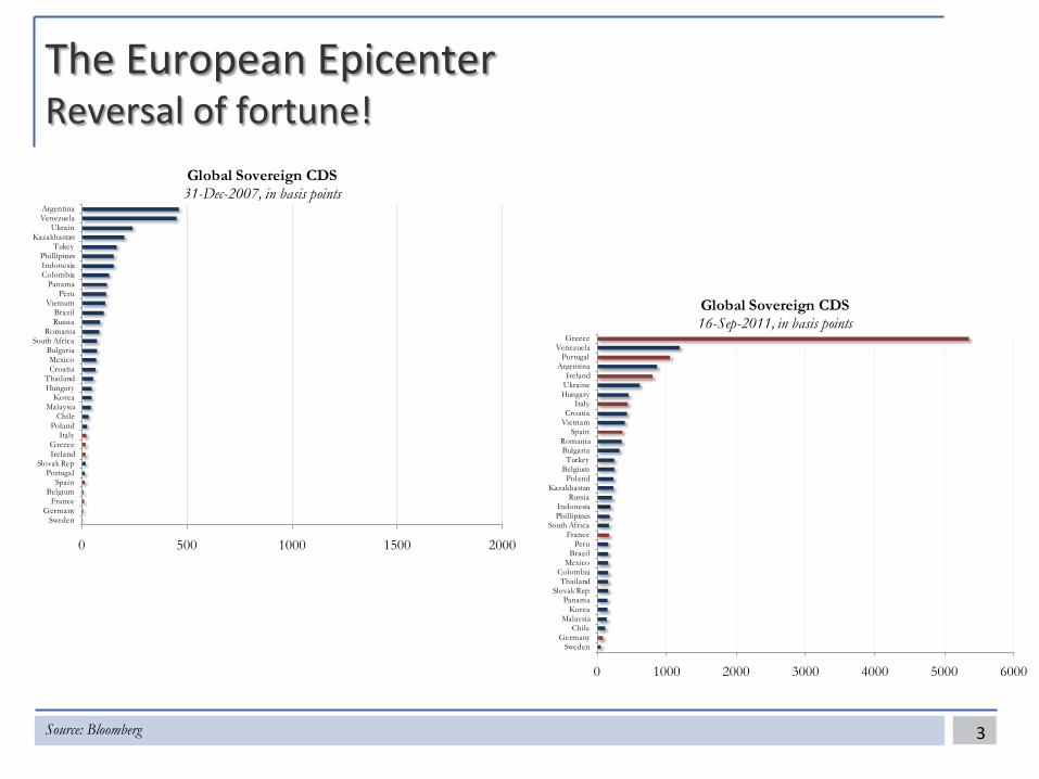
The European EpicenterReversal of fortune!

3Source: Bloomberg

0 500 1000 1500 2000

SwedenGermany

FranceBelgium

SpainPortugal

Slovak RepIrelandGreece

ItalyPoland

ChileMalaysia

KoreaHungaryThailand

CroatiaMexico

BulgariaSouth Africa

RomaniaRussiaBrazil

VietnamPeru

PanamaColombiaIndonesiaPhillipines

TukeyKazakhastan

UkrainVenezuelaArgentina

Global Sovereign CDS31-Dec-2007, in basis points

0 1000 2000 3000 4000 5000 6000

SwedenGermany

ChileMalaysia

KoreaPanama

Slovak RepThailand

ColombiaMexico

BrazilPeru

FranceSouth Africa

PhillipinesIndonesia

RussiaKazakhastan

PolandBelgiumTurkey

BulgariaRomania

SpainVietnamCroatia

ItalyHungaryUkraineIreland

ArgentinaPortugal

VenezuelaGreece

Global Sovereign CDS16-Sep-2011, in basis points

The European epicenterOne currency, 17 sovereign debt issuers

4Source: Bloomberg

-5%

0%

5%

10%

15%

20%

25%

Mar

-93

Apr-9

4

May

-95

Jun-

96

Jul-9

7

Aug-

98

Sep-

99

Oct

-00

Nov

-01

Jan-0

3

Feb-

04

Mar

-05

Apr-0

6

May

-07

Jun-

08

Jul-0

9

Aug-

10

Sep-

11

Spreads Over German BondsIn %

Official Launch of the EuroPortugal

Greece

Ireland

France

Italy

Spain

The European epicenterStructural heterogeneity and the CGD trap

5

80

100

120

140

160

180

200

Q1-

2000

Q3-

2000

Q1-

2001

Q3-

2001

Q1-

2002

Q3-

2002

Q1-

2003

Q3-

2003

Q1-

2004

Q3-

2004

Q1-

2005

Q3-

2005

Q1-

2006

Q3-

2006

Q1-

2007

Q3-

2007

Q1-

2008

Q3-

2008

Q1-

2009

Q3-

2009

Q1-

2010

Q3-

2010

Q1-

2011

Unit Labor Costs in EuropeIndex base 100 = q1-2000

GermanyItalyPortugalGreeceFranceSpain

-10.0%

-5.0%

0.0%

5.0%

10.0%

15.0%

20.0%

Greece France Ireland Portugal Italy Spain

% o

f G

DP

Debt Sustainability in EuropeTheoretical vs Actual Primary Balance

Actual

Theoretical

Source: EuroStats and Bloomberg. For panel B, the theoretical primary balances is calculated using the last observation of the nominal interests rates on 10ys bonds, and assuming a long term inflation and growth of 1.5% and 2%, respectively.

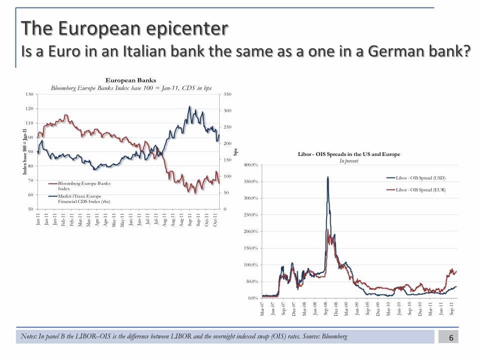
The European epicenterIs a Euro in an Italian bank the same as a one in a German bank?

6Notes: In panel B the LIBOR–OIS is the difference between LIBOR and the overnight indexed swap (OIS) rates. Source: Bloomberg

0.0%

50.0%

100.0%

150.0%

200.0%

250.0%

300.0%

350.0%

400.0%

Mar

-07

Jun-

07

Sep-

07

Dec

-07

Mar

-08

Jun-

08

Sep-

08

Dec

-08

Mar

-09

Jun-

09

Sep-

09

Dec

-09

Mar

-10

Jun-

10

Sep-

10

Dec

-10

Mar

-11

Jun-

11

Sep-

11

Libor - OIS Spreads in the US and EuropeIn percent

Libor - OIS Spread (USD)

Libor - OIS Spread (EUR)

0

50

100

150

200

250

300

350

50

60

70

80

90

100

110

120

130

Jan-

11

Jan-

11

Jan-

11

Feb-

11

Feb-

11

Mar

-11

Mar

-11

Apr-1

1

Apr-1

1

May

-11

May

-11

Jun-

11

Jun-

11

Jul-1

1

Jul-1

1

Aug-

11

Aug-

11

Aug-

11

Sep-

11

Sep-

11

Oct

-11

Oct

-11

bps

Inde

x bas

e 100

= Ja

n-11

European BanksBloomberg Europe Banks Index base 100 = Jan-11, CDS in bps

Bloomberg Europe Banks Index

Markit iTraxx Europe Financial CDS Index (rhs)

The US epicenterFeeble growth prospects: Keynes vs. Fischer

7Sources: Consensus Forecasts (October 2011) and Bloomberg.

90

95

100

105

110

115

120

125

130

135

Mar

-03

Nov

-03

Jul-0

4

Mar

-05

Nov

-05

Jul-0

6

Mar

-07

Nov

-07

Jul-0

8

Mar

-09

Nov

-09

Jul-1

0

Mar

-11

Nov

-11

Jul-1

2

Mar

-13

Inde

x ba

se 10

0 =

Iq -

2003

US Economic ActivityGDP Index base 100 = Iq - 2003

2003-2007 trend

-20.0%

-15.0%

-10.0%

-5.0%

0.0%

5.0%

10.0%

0

10

20

30

40

50

60

70

Jan-

06A

pr-0

6Ju

l-06

Oct

-06

Jan-

07A

pr-0

7Ju

l-07

Oct

-07

Jan-

08A

pr-0

8Ju

l-08

Oct

-08

Jan-

09A

pr-0

9Ju

l-09

Oct

-09

Jan-

10A

pr-1

0Ju

l-10

Oct

-10

Jan-

11A

pr-1

1Ju

l-11

Oct

-11

Indu

stri

al P

rodu

ctio

n (Y

oY)

ISM

Inde

x

Industrial Production and ISM IndexIndustrial Production (YoY %)

ISM Index Series2

The US EpicenterDowngraded but still the safe haven (“exorbitant privilege”)

8Source: Bloomberg

90

95

100

105

110

115

Dec

-10

Jan-

11

Mar

-11

Apr

-11

May

-11

Jun-

11

Jul-1

1

Aug

-11

Sep-

11

Currencies: 2011Index base 100 = 1-Jan-2011

Japan UK

US-EUR Brazil

1.5%

2.0%

2.5%

3.0%

3.5%

4.0%

1200

1300

1400

1500

1600

1700

1800

1900

2000

Jan-

11

Jan-

11

Feb-

11

Feb-

11

Mar

-11

Mar

-11

Apr

-11

Apr

-11

May

-11

May

-11

May

-11

Jun-

11

Jun-

11

Jul-1

1

Jul-1

1

Aug

-11

Aug

-11

Sep-

11

Perc

ent

USD

Gold and US T10 2011

Gold

US T10 (rhs)

Short-run scenarios 1. Continued real de-coupling

2. A great global re-coupling

9

Real cyclical de-coupling has been a salient feature of the post-crisis global economic landscape…

10Note: The group of developed countries refers to OECD countries excluding Turkey, Mexico, Republic of Korea, and Central European countries. Source: CPB (Netherlands Bureau for Economic Policy Analysis).

80

85

90

95

100

105

110

115

120

Jan-

06

Aug-

06

Mar

-07

Oct-0

7

May

-08

Dec-

08

Jul-0

9

Feb-

10

Sep-

10

Apr-1

1

World Industrial ProductionIndex Apr-08 = 100

CrisisAdvanced EconomiesEmerging Economies

51%38%

27%

34%44%

57%

8% 7% 8%8% 11% 8%

0%

20%

40%

60%

80%

100%

1996-2001 2001-2006 2009-2011

Contribution to World Economic GDPas a % of World GDP increase (PPP)

Others Other Advanced EconomiesEM - 20 Euro (15)+US+Japan+Canada+UK

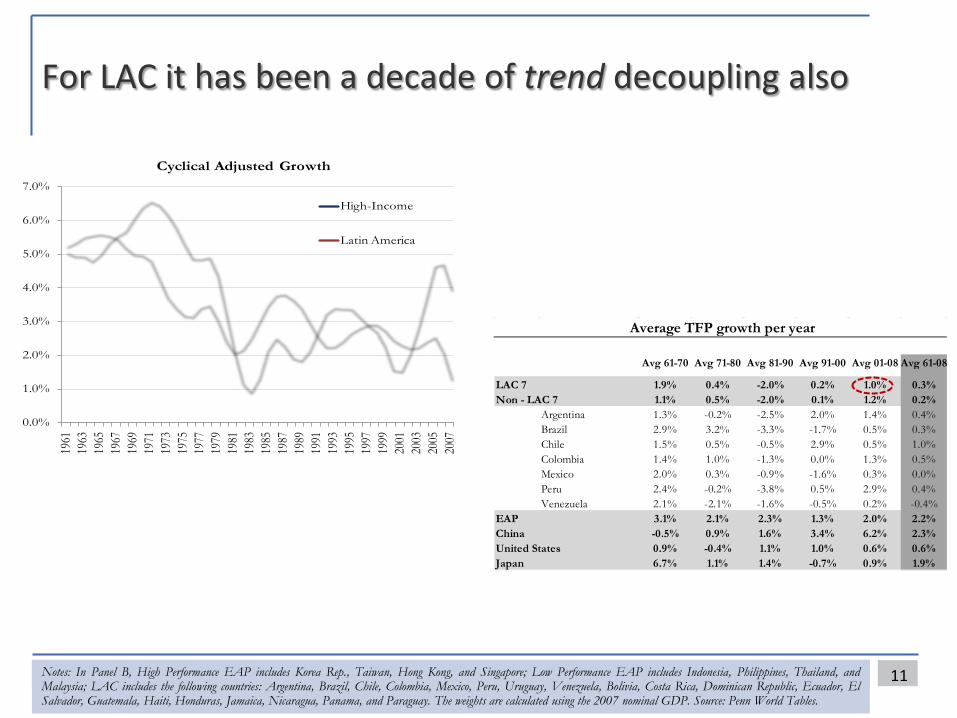
For LAC it has been a decade of trend decoupling also

11Notes: In Panel B, High Performance EAP includes Korea Rep., Taiwan, Hong Kong, and Singapore; Low Performance EAP includes Indonesia, Philippines, Thailand, andMalaysia; LAC includes the following countries: Argentina, Brazil, Chile, Colombia, Mexico, Peru, Uruguay, Venezuela, Bolivia, Costa Rica, Dominican Republic, Ecuador, ElSalvador, Guatemala, Haiti, Honduras, Jamaica, Nicaragua, Panama, and Paraguay. The weights are calculated using the 2007 nominal GDP. Source: Penn World Tables.

0.0%

1.0%

2.0%

3.0%

4.0%

5.0%

6.0%

7.0%

1961

1963

1965

1967

1969

1971

1973

1975

1977

1979

1981

1983

1985

1987

1989

1991

1993

1995

1997

1999

2001

2003

2005

2007

Cyclical Adjusted Growth

High-Income

Latin America

Avg 61-70 Avg 71-80 Avg 81-90 Avg 91-00 Avg 01-08 Avg 61-08

LAC 7 1.9% 0.4% -2.0% 0.2% 1.0% 0.3%Non - LAC 7 1.1% 0.5% -2.0% 0.1% 1.2% 0.2%

Argentina 1.3% -0.2% -2.5% 2.0% 1.4% 0.4%Brazil 2.9% 3.2% -3.3% -1.7% 0.5% 0.3%Chile 1.5% 0.5% -0.5% 2.9% 0.5% 1.0%Colombia 1.4% 1.0% -1.3% 0.0% 1.3% 0.5%Mexico 2.0% 0.3% -0.9% -1.6% 0.3% 0.0%Peru 2.4% -0.2% -3.8% 0.5% 2.9% 0.4%Venezuela 2.1% -2.1% -1.6% -0.5% 0.2% -0.4%

EAP 3.1% 2.1% 2.3% 1.3% 2.0% 2.2%China -0.5% 0.9% 1.6% 3.4% 6.2% 2.3%United States 0.9% -0.4% 1.1% 1.0% 0.6% 0.6%Japan 6.7% 1.1% 1.4% -0.7% 0.9% 1.9%

Average TFP growth per year

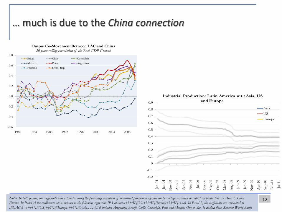
… much is due to the China connection

12

-0.2

-0.1

0

0.1

0.2

0.3

0.4

0.5

0.6

0.7

0.8

0.9

Jan-0

4

Jun-

04

Nov

-04

Apr-0

5

Sep-

05

Feb-

06

Jul-0

6

Dec

-06

May

-07

Oct

-07

Mar

-08

Aug-

08

Jan-0

9

Jun-

09

Nov

-09

Apr-1

0

Sep -

10

Feb-

11

Jul-1

1

Industrial Production: Latin America w.r.t Asia, US and Europe

AsiaUSEurope

Notes: In both panels, the coefficients were estimated using the percentage variation of industrial production against the percentage variation in industrial production in Asia, US and Europe. In Panel A the coefficients are associated to the following regression IP Latam=a+b1*IP(US)+b2*IP(Europe)+b3*IP(Asia). In Panel B, the coefficients are associated to IPLAC 6=a+b1*IP(US)+b2*IP(Europe)+b3*IP(Asia). LAC 6 includes Argentina, Brazil, Chile, Colombia, Peru and Mexico. One st .dev. in dashed lines. Sources: World Bank.

-0.6

-0.4

-0.2

0.0

0.2

0.4

0.6

0.8

1980 1984 1988 1992 1996 2000 2004 2008

Output Co-Movement Between LAC and China20 years rolling correlation of the Real GDP Growth

Brazil Chile ColombiaMexico Peru ArgentinaPanama Dom. Rep.

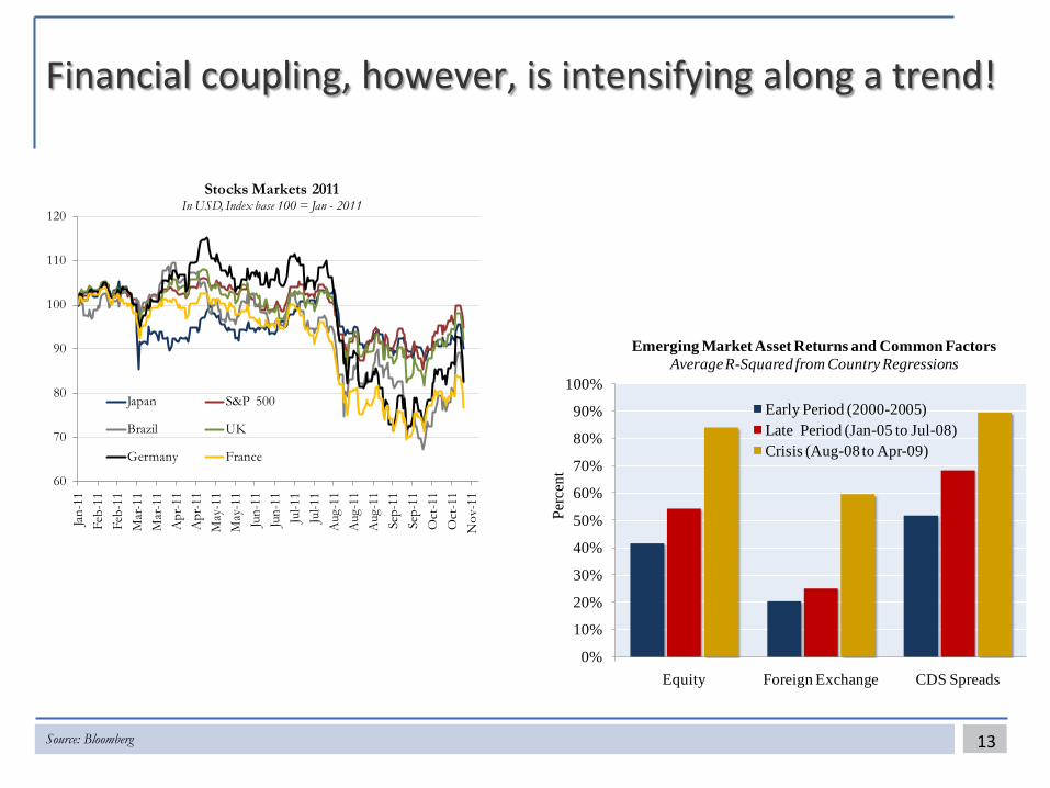
Financial coupling, however, is intensifying along a trend!

13Source: Bloomberg

0%

10%

20%

30%

40%

50%

60%

70%

80%

90%

100%

Equity Foreign Exchange CDS Spreads

Perc

ent

Emerging Market Asset Returns and Common Factors Average R-Squared from Country Regressions

Early Period (2000-2005)Late Period (Jan-05 to Jul-08)Crisis (Aug-08 to Apr-09)

60

70

80

90

100

110

120

Jan-

11Fe

b-11

Feb-

11M

ar-1

1M

ar-1

1A

pr-1

1A

pr-1

1M

ay-1

1M

ay-1

1Ju

n-11

Jun-

11Ju

l-11

Jul-1

1A

ug-1

1A

ug-1

1A

ug-1

1Se

p-11

Sep-

11O

ct-1

1O

ct-1

1N

ov-1

1

Stocks Markets 2011In USD, Index base 100 = Jan - 2011

Japan S&P 500

Brazil UK

Germany France

14Source: Bloomberg

0

10

20

30

40

50

60

70

80

90

Aug

-05

Dec

-05

Mar

-06

Jun-

06Se

p-06

Dec

-06

Mar

-07

Jun-

07Se

p-07

Dec

-07

Mar

-08

Jun-

08Se

p-08

Dec

-08

Mar

-09

Jun-

09Se

p-09

Dec

-09

Mar

-10

Jun-

10Se

p-10

Dec

-10

Mar

-11

Jun-

11Se

p-11

Dec

-11

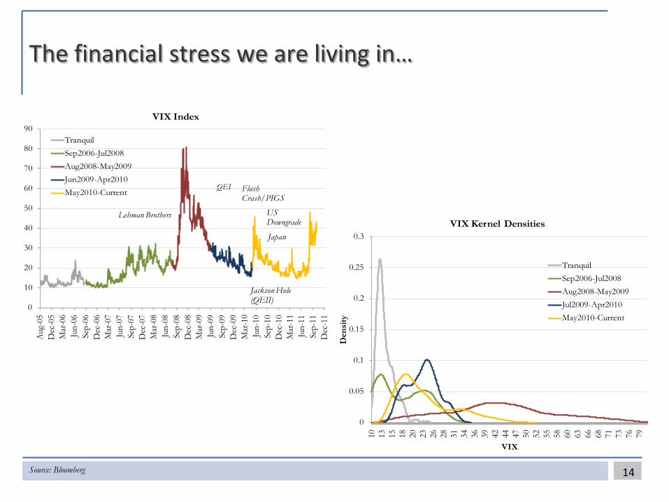
VIX Index

Tranquil Sep2006-Jul2008Aug2008-May2009Jun2009-Apr2010May2010-Current

Lehman Brothers

QEI Flash Crash/PIGS

Jackson Hole (QEII)

Japan

US Downgrade

0

0.05

0.1

0.15

0.2

0.25

0.3

10 13 15 18 20 23 26 28 31 34 36 39 42 44 47 50 52 55 58 60 63 66 68 71 73 76 79

Den

sity

VIX

VIX Kernel Densities

TranquilSep2006-Jul2008Aug2008-May2009Jul2009-Apr2010May2010-Current

The financial stress we are living in…

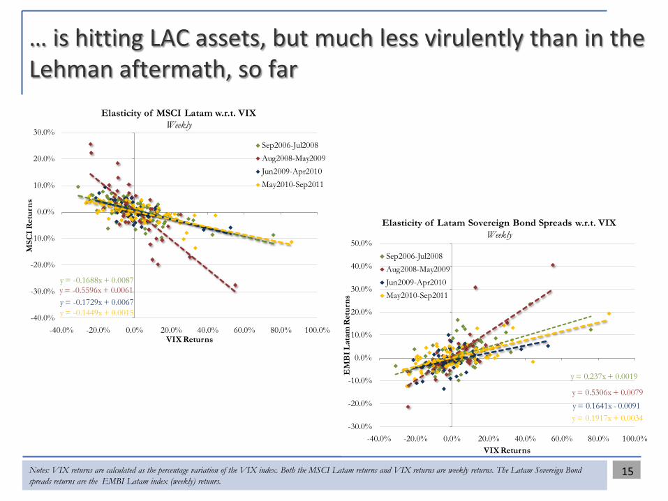
15Notes: VIX returns are calculated as the percentage variation of the VIX index. Both the MSCI Latam returns and VIX returns are weekly returns. The Latam Sovereign Bond spreads returns are the EMBI Latam index (weekly) retunrs.

y = -0.1688x + 0.0087y = -0.5596x + 0.0061y = -0.1729x + 0.0067y = -0.1449x + 0.0015-40.0%

-30.0%

-20.0%

-10.0%

0.0%

10.0%

20.0%

30.0%

-40.0% -20.0% 0.0% 20.0% 40.0% 60.0% 80.0% 100.0%

MSC

I Ret

urns

VIX Returns

Elasticity of MSCI Latam w.r.t. VIXWeekly

Sep2006-Jul2008Aug2008-May2009Jun2009-Apr2010May2010-Sep2011

y = 0.237x + 0.0019

y = 0.5306x + 0.0079y = 0.1641x - 0.0091y = 0.1917x + 0.0034

-30.0%

-20.0%

-10.0%

0.0%

10.0%

20.0%

30.0%

40.0%

50.0%

-40.0% -20.0% 0.0% 20.0% 40.0% 60.0% 80.0% 100.0%

EM

BI L

atam

Ret

urns

VIX Returns

Elasticity of Latam Sovereign Bond Spreads w.r.t. VIXWeekly


… is hitting LAC assets, but much less virulently than in the Lehman aftermath, so far

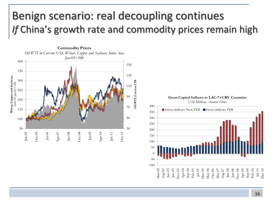
Benign scenario: real decoupling continuesIf China’s growth rate and commodity prices remain high

16

30

50

70

90

110

130

150

50

100

150

200

250

300

350

400

Jan-

05

Oct

-05

Jul-0

6

Apr

-07

Jan-

08

Oct

-08

Jul-0

9

Apr

-10

Jan-

11

Oct

-11

Oil

WT

I, C

urre

nt U

S$

Whe

at, C

oppe

r and

Soy

bean

, In

dex

01-Ja

n-05

=10

0

Commodity PricesOil WTI in Current US$, Wheat, Copper and Soybean: Index base

Jan-05=100

-100

-50

0

50

100

150

200

250

300

350

400

Mar

-02

Aug

-02

Jan-

03Ju

n-03

Nov

-03

Apr

-04

Sep-

04Fe

b-05

Jul-0

5D

ec-0

5M

ay-0

6O

ct-0

6M

ar-0

7A

ug-0

7Ja

n-08

Jun-

08N

ov-0

8A

pr-0

9Se

p-09

Feb-

10Ju

l-10

Dec

-10

Gross Capital Inflows to LAC-7+URY Countries US$ Millions, Annual Flows

Gross Inflows Non-FDI Gross Inflows FDI

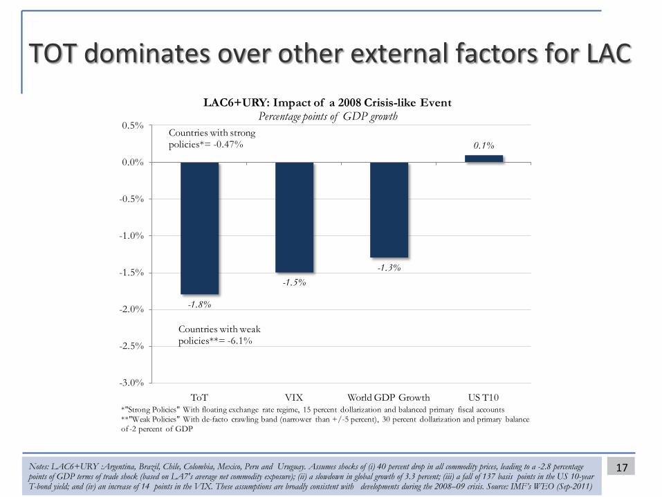
TOT dominates over other external factors for LAC

17Notes: LAC6+URY :Argentina, Brazil, Chile, Colombia, Mexico, Peru and Uruguay. Assumes shocks of (i) 40 percent drop in all commodity prices, leading to a -2.8 percentage points of GDP terms of trade shock (based on LA7's average net commodity exposure); (ii) a slowdown in global growth of 3.3 percent; (iii) a fall of 137 basis points in the US 10-year T-bond yield; and (iv) an increase of 14 points in the VIX. These assumptions are broadly consistent with developments during the 2008–09 crisis. Source: IMF’s WEO (Sep-2011)

-1.8%

-1.5%-1.3%

0.1%

-3.0%

-2.5%

-2.0%

-1.5%

-1.0%

-0.5%

0.0%

0.5%

ToT VIX World GDP Growth US T10

LAC6+URY: Impact of a 2008 Crisis-like EventPercentage points of GDP growth

Countries with weak policies**= -6.1%

*"Strong Policies" With floating exchange rate regime, 15 percent dollarization and balanced primary fiscal accounts**"Weak Policies" With de-facto crawling band (narrower than +/-5 percent), 30 percent dollarization and primary balance of -2 percent of GDP

Countries with strong policies*= -0.47%

Forecasts are being revised downward world-wide, but so far seem to be assuming a benign scenario

18Source: Consensus Forecasts (2011)

0%

1%

2%

3%

4%

5%

6%

7%

8%

9%

10%

EEUU EuroZone China Latin America South East Asia Eastern Europe

GDP Growth Forecasts EvolutionForecasts for 2012

January 2011

October 2011

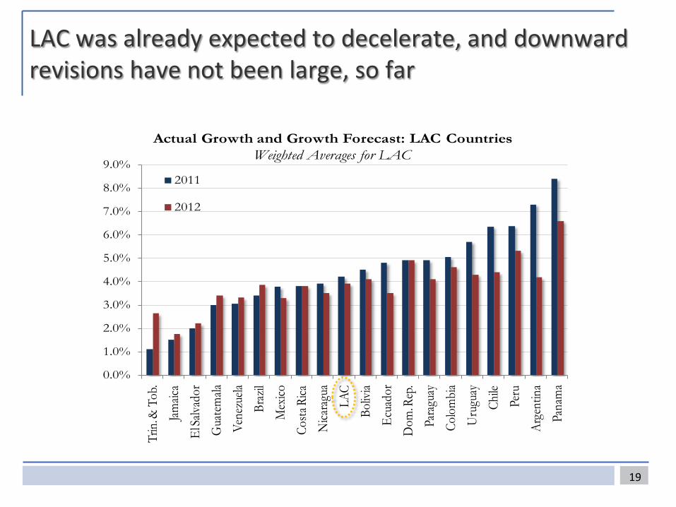
LAC was already expected to decelerate, and downward revisions have not been large, so far

19

0.0%

1.0%

2.0%

3.0%

4.0%

5.0%

6.0%

7.0%

8.0%

9.0%Tr

in. &

Tob

.Jam

aica

El Sa

lvado

rG

uate

mala

Vene

zuela

Braz

ilM

exico

Costa

Rica

Nica

ragu

aLA

CBo

livia

Ecua

dor

Dom

. Rep

.Pa

ragu

ayCo

lom

bia

Uru

guay

Chile

Peru

Arge

ntin

aPa

nam

a

Actual Growth and Growth Forecast: LAC CountriesWeighted Averages for LAC

2011

2012

Bad scenario: a global downward re-coupling

In this scenario, major tail risks materialize and another great recession ensues

All transmission channels would be activated Terms of trade

External demand for LAC exports of goods and services

Remittances

Financial channels

LAC countries that have the greatest shock absorption capacity are not necessarily those with the greatest growth potential Mexico versus Argentina

20

Bad scenario: a global downward re-couplingLines of defense in shock absorption

Robust monetary policy frameworks in LAC, mostly Shock absorption via e-rate flexibility/monetary policy independence

Rate increases over the past 15 month gives the region room to maneuver

How good are LAC’s fiscal buffers? Comfortable public debt situation but insufficient fiscal flexibility

Much less space among Central American and Caribbean countries

How good are LAC’s financial system buffers? Strong capital and liquidity positions, except in the Caribbean

Have systemic risks been brewing in the past year or so?

How good are LAC’s social safety nets? Ability to scale up social assistance programs vary widely in the region

Social insurance frameworks are the weak link

21

22

Thank you

LAC’s success A decade of high growth and progress in social equity

23Source: LCSPP based on Socio-Economic Database for Latin America and the Caribbean (CEDLAS and The World Bank).

-0.1 -0.05 0 0.05 0.1

ParaguayPeru

BrazilMexico

Latin AmericaPanama

ArgentinaEl Salvador

ChileBolivia

HondurasUruguay

ColombiaDominican Republic

Costa Rica

Gini Coefficient Cumulative ChangeFrom 2009 to 1995

3,000

4,000

5,000

6,000

7,000

8,000

9,000

10,000

20

25

30

35

40

45

1994

1996

1998

2000

2002

2004

2006

2008

2010

GDP P

er C

apita

US

Doll

ars

Mod

erat

e Pov

erty

Rat

e US

$ 4 a

Day

Per Capita GDP Growth and Poverty LAC Countries

Poverty Headcount GDP Per Capita

Cyclical-adjusted Growth in Latin America and High-Income CountriesTrend growth computed using the band-pass filter

0%

1%

2%

3%

4%

5%

6%

7%

1961 1964 1967 1970 1973 1976 1979 1982 1985 1988 1991 1994 1997 2000 2003 2006 2009

High-Income

Latin America

LAC: Expanding Middle Class

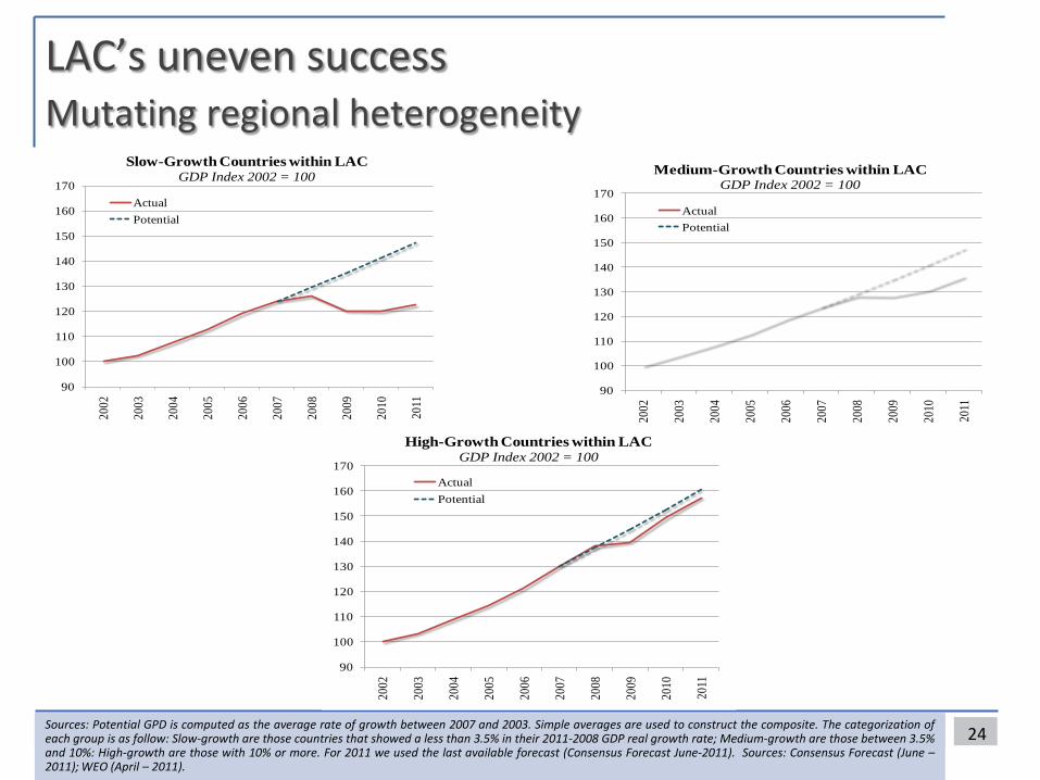
LAC’s uneven successMutating regional heterogeneity

24Sources: Potential GPD is computed as the average rate of growth between 2007 and 2003. Simple averages are used to construct the composite. The categorization ofeach group is as follow: Slow-growth are those countries that showed a less than 3.5% in their 2011-2008 GDP real growth rate; Medium-growth are those between 3.5%and 10%: High-growth are those with 10% or more. For 2011 we used the last available forecast (Consensus Forecast June-2011). Sources: Consensus Forecast (June –2011); WEO (April – 2011).

90

100

110

120

130

140

150

160

170

2002

2003

2004

2005

2006

2007

2008

2009

2010

2011

Slow-Growth Countries within LACGDP Index 2002 = 100

ActualPotential

90

100

110

120

130

140

150

160

170

2002

2003

2004

2005

2006

2007

2008

2009

2010

2011

Medium-Growth Countries within LACGDP Index 2002 = 100

ActualPotential

90

100

110

120

130

140

150

160

170

2002

2003

2004

2005

2006

2007

2008

2009

2010

2011

High-Growth Countries within LACGDP Index 2002 = 100

ActualPotential

LAC’s uneven successWhere you are matters less than to whom you are connected

25Sources: World Bank’s World Development Indicators – WDI (December 2010), IMF's World Economic Outlook – WEO (April 2011), and Consensus Forecasts (June 2011) –Latest available forecasts. Potential GDP is calculated computing the annual average real growth rate for the 2002-2007 to 2007 GDP. Weighted averages (2007 NominalGDP in USD Billions).

Low growth (<4%): St. Kitts and Nevis, Antigua and Barbuda, Grenada, Barbados, Jamaica, Bahamas, Venezuela, Trinidad and Tobago, St. Vincent and the Grenadines, El Salvador, St. Lucia, Dominica and Mexico

Medium growth (4%-10%): Honduras, Belize, Haiti, Nicaragua, Guatemala, Costa Rica and Ecuador

High growth (>10%): Chile, Colombia, Brazil, Guyana, Bolivia, Suriname, Paraguay, Dominican Republic, Peru, Argentina, Uruguay and Panama

Number of countries

Mean growth 2003-2007*

Mean Growth 2003-2011

Mean Growth 2008-2011**

Max. 2008-2011

Min. 2008-2011

Low growth 13 4.4% 2.3% -0.3% 3.3% -12.3%Medium growth 7 4.4% 3.5% 2.4% 7.9% 4.1%High growth 12 5.4% 5.2% 4.9% 18.8% 10.0%Total 32 4.8% 3.7% 2.2% 18.8% -12.3%* This is the measure used to construct the "Potential GDP"

** This is the measure used to define the classification as "Low", "Medium" and "High".

Cumulative

VIX dominates stock market co-movement in crisis times

26Notes: The coefficient showed in both panels are associated to the following regression MSCI Latam returns=a+b1*VIX returns+b2*S&P500 returns.

MSCI LatAm Returns = a+b1*VIX+b2*S&P500

(0.0263)-0.174

-0.012-0.059

-0.200

-0.150

-0.100

-0.050

0.000

0.050

0.100

Coefficient of VIX

MSCI Latam w.r.t VIX and S&P500: VIX CoefficientRobust standar errors in parentheses


-0.056

(0.073)

(0.019)

(0.025)

1.012 1.197 1.3530.719

-0.200

0.000

0.200

0.400

0.600

0.800

1.000

1.200

1.400

1.600

1.800

Coefficient SP500

MSCI Latam w.r.t VIX and S&P500: S&P500 Coefficient Robust standar errors in parentheses


(0.212)

(0.195)

(0.132)

(0.213)

global scenarios for lac - world...

Documents