global land cover mapping from modis: algorithms and early results

Global land cover mapping from MODIS: algorithms and early results

M.A. Friedl a,*, D.K. McIver a, J.C.F. Hodges a, X.Y. Zhang a, D. Muchoney b, A.H. Strahler a,C.E. Woodcock a, S. Gopal a, A. Schneider a, A. Cooper a, A. Baccini a, F. Gao a, C. Schaaf a

aDepartment of Geography and Center for Remote Sensing, Boston University, 675 Commonwealth Avenue, Boston, MA 02215, USAbConservation International, 1919 M Street, NW Suite 600, Washington, DC 20036, USA

Received 6 April 2001; received in revised form 4 December 2001; accepted 10 February 2002

Abstract

Until recently, advanced very high-resolution radiometer (AVHRR) observations were the only viable source of data for global land cover

mapping. While many useful insights have been gained from analyses based on AVHRR data, the availability of moderate resolution imaging

spectroradiometer (MODIS) data with greatly improved spectral, spatial, geometric, and radiometric attributes provides significant new

opportunities and challenges for remote sensing-based land cover mapping research. In this paper, we describe the algorithms and databases

being used to produce the MODIS global land cover product. This product provides maps of global land cover at 1-km spatial resolution

using several classification systems, principally that of the IGBP. To generate these maps, a supervised classification methodology is used that

exploits a global database of training sites interpreted from high-resolution imagery in association with ancillary data. In addition to the IGBP

class at each pixel, the MODIS land cover product provides several other parameters including estimates for the classification confidence

associated with the IGBP label, a prediction for the most likely alternative class, and class labels for several other classification schemes that

are used by the global modeling community. Initial results based on 5 months of MODIS data are encouraging. At global scales, the

distribution of vegetation and land cover types is qualitatively realistic. At regional scales, comparisons among heritage AVHRR products,

Landsat TM data, and results from MODIS show that the algorithm is performing well. As a longer time series of data is added to the

processing stream and the representation of global land cover in the site database is refined, the quality of the MODIS land cover product will

improve accordingly.

D 2002 Elsevier Science Inc. All rights reserved.

1. Introduction

Land cover, and human and natural alteration of land

cover, play a major role in global-scale patterns of the

climate and biogeochemistry of the earth system. Terres-

trial ecosystems exert considerable control on the planet’s

biogeochemical cycles, which in turn significantly influ-

ence the climate system through the radiative properties

of greenhouse gases and reactive species. Further, varia-

tions in topography, albedo, vegetation cover, and other

physical characteristics of the land surface influence sur-

face–atmosphere fluxes of sensible heat, latent heat, and

momentum, which in turn influence weather and climate

(Sellers et al., 1997).

Until recently, land-cover data sets used within models of

global climate and biogeochemistry were derived from

preexisting maps and atlases. The most commonly used

data sets were compiled by Olson and Watts (1982),

Matthews (1983), and Wilson and Henderson-Sellers

(1985). While these (and other) data sources provided the

best available source of information regarding the distribu-

tion of global land cover at the time, several limitations are

inherent in their use. For example, global land cover is

intrinsically dynamic. Therefore, the source data upon

which these maps were compiled is now out of date in

many areas. Further, each of these data sets utilize different

spatial scales and classification schemes, which are gener-

ally different from those required by contemporary models.

As a result, confusion regarding how the reference class

units are translated to the classification system and scale

used by a model can lead to errors in the final product. For

example, floristic and climatically based classifications,

while not inherently compatible, may need to be combined

0034-4257/02/$ - see front matter D 2002 Elsevier Science Inc. All rights reserved.

PII: S0034 -4257 (02 )00078 -0

* Corresponding author. Tel.: +1-617-353-5745.

E-mail address: [email protected] (M.A. Friedl).

www.elsevier.com/locate/rse

Remote Sensing of Environment 83 (2002) 287–302

and reclassified to generate physiognomic cover types

(Townshend, Justice, Li, Gurney, & MacManus, 1991).

Finally, conventional land cover data sets such as those

mentioned above often provide maps of potential vegetation

inferred from climatic variables such as temperature and

precipitation. In many regions, especially where humans

have dramatically modified the landscape, the true vegeta-

tion type or land cover can deviate significantly from the

potential vegetation.

More recently, remote sensing has been used as a basis

for mapping global land cover using data from the advanced

very high-resolution radiometer (AVHRR). The first global

land cover map compiled from remote sensing was pro-

duced by DeFries and Townshend (1994) using maximum

likelihood classification of monthly composited AVHRR

normalized difference vegetation index (NDVI) data at 1jspatial resolution. Subsequently, DeFries, Hansen, Tow-

hsend, and Sohlberg (1998) used a decision tree classifica-

tion technique to produce a map of global land cover at

8-km spatial resolution, again from AVHRR data. Most

recently, Loveland et al. (2000) used unsupervised classi-

fication of monthly composited AVHRR NDVI data

acquired between April 1992 and March 1993 to map global

land cover at 1-km spatial resolution. Hansen, DeFries,

Townshend, and Sohlberg (2000) used the same AVHRR

data set, but adopted a supervised classification strategy

using decision trees. Prior to the availability of newer, high

quality data sets from instruments onboard the Terra (and

other) space craft, data sets derived from the AVHRR

provided the best available remote sensing-based maps of

global land cover. However, because the information con-

tent of AVHRR data is limited for land cover mapping

applications, numerous uncertainties are present in these

maps (Loveland et al., 1999).

The moderate resolution imaging spectroradiometer

(MODIS) on-board Terra includes seven spectral bands

that are explicitly designed for land applications, and data

from MODIS is now available for land cover mapping

applications. The enhanced spectral, spatial, radiometric,

and geometric quality of MODIS data provides a greatly

improved basis for monitoring and mapping global land

cover relative to AVHRR data. Further, the algorithms

being used with MODIS data have been designed for

operational mapping, thereby providing rapid turn-around

between data acquisition and map production. The time-

liness and quality of land cover maps produced from

MODIS should, therefore, be useful for a wide array of

scientific applications that require land cover information at

regional to global scales.

In this paper, we describe global land cover mapping

activities being conducted using data from MODIS. The

first objective of this paper is to provide an overview of the

MODIS land cover product, describing the main elements of

the classification methodologies and databases being used to

map global land cover from MODIS data. As part of this

discussion, we provide information regarding algorithm

assessment and validation. The second objective is to

provide a summary of early results at both global and

regional scales, and to highlight specific successes, lessons

learned, and areas of ongoing research.

2. Algorithm description

The MODIS global land cover product suite includes two

main parameters. The first parameter provides global land

cover at 1-km spatial resolution updated at quarterly (96-

day) intervals (Strahler et al., 1999; Friedl et al., 2000a).

Note that because land cover is largely static at this time

scale, early quarterly releases will effectively represent

revisions to the existing map. Subsequent releases should

stabilize rapidly, and once this happens, we anticipate

scaling back to annual or semiannual updates. These

updates will reflect improvements to the global land cover

map arising from continued site database development,

refinements to the classification algorithm, and feedback

regarding map quality from the user community and vali-

dation activities. In addition to the 1-km maps, the MODIS

global land cover product is also being provided at coarser

resolution (nominally 28 km c 1/4j) to serve the needs of

the global modeling community who typically require

spatial resolutions much coarser than 1 km. As part of

this data set, the sub-grid scale frequency distribution for

each class is included to provide information regarding

fine resolution spatial variability in land cover within each

1/4j cell.

The second parameter, land cover dynamics, provides a

measure of land cover change, again at 1-km spatial

resolution, but at annual time scales. This product employs

a change-vector algorithm (Lambin & Strahler, 1994a,b) to

describe land cover change, and requires two full years of

data for product generation. Note that this parameter is

designed to identify areas where land surface properties

exhibit change, independent of land cover (e.g., drought or

interannual variation in biospheric response to climate

forcing). Because substantially less than one full year of

MODIS data is available at the time of this writing, this

paper emphasizes the static MODIS land cover product.

Within this context, it is important to note that the MODIS

global land cover product discussed in this paper is distinct

from the MODIS vegetation cover conversion and vegeta-

tion continuous fields products, which address different

aspects of land cover and are described in other papers

within this volume.

The MODIS land cover classification algorithm

(MLCCA) uses a supervised classification methodology

(Schowengerdt, 1997) and includes two key elements.

First, the algorithm utilizes a database of sites distributed

globally that provides exemplars of each land cover type

(and subpopulations within each type). Second, supervised

classification algorithms are used to classify the high-

dimensional (multispectral and multitemporal) data pro-

M.A. Friedl et al. / Remote Sensing of Environment 83 (2002) 287–302288

vided by MODIS. Thus, implementation of the MLCCA

involved substantial challenges in terms of both compiling

a globally representative database of sites for classifier

training, and in implementing algorithms that overcome

previously unconsidered challenges involved in classifying

high data volumes with complex feature attributes at global

scales. In the sections that follow, we describe these

methods in more detail.

2.1. Land cover units

The primary objective of the MODIS land cover product

is to facilitate the inference of biophysical information for

use in regional and global modeling studies. Thus, the

specific classification units of land cover need to be both

discernible with high accuracy from remotely sensed and

ancillary data, and directly related to physical characteristics

of the surface, especially vegetation. A set of 17 such land

cover classes was developed by the International Geo-

sphere-Biosphere Programme Data and Information System

(IGBP-DIS) specifically for this purpose (Loveland & Bel-

ward, 1997). Since the IGBP system of units was developed

for a global land cover product at a similar resolution and

for similar purposes (biophysical parameterization for mod-

eling), the IGBP classification is also used in the MODIS

land cover product.

Table 1 provides a list of the IGBP land cover units with

accompanying descriptions. The list includes 11 classes of

natural vegetation, 3 classes of developed and mosaic lands,

and 3 classes of nonvegetated lands. The natural vegetation

units distinguish evergreen and deciduous, broadleaf and

needleleaf forests, where one of each pair of attributes

dominates; mixed forests, where mixtures occur; closed

shrublands and open shrublands; savannas and woody

savannas; grasslands; and permanent wetlands of large areal

extent. The three classes of developed and mosaic lands

distinguish among croplands, urban and built-up lands, and

cropland/natural vegetation mosaics. Classes of nonvege-

Table 1

The IGBP classification scheme (the number in parentheses after the name of each class indicates the number of STEP sites for each class)

IGBP land cover units

Natural vegetation

Evergreen needleleaf forests (127) Lands dominated by needleleaf woody vegetation with a percent cover >60% and height exceeding 2 m.

Almost all trees remain green all year. Canopy is never without green foliage.

Evergreen broadleaf forests (201) Lands dominated by broadleaf woody vegetation with a percent cover >60% and height exceeding 2 m.

Almost all trees and shrubs remain green year round. Canopy is never without green foliage.

Deciduous needleleaf forests (16) Lands dominated by woody vegetation with a percent cover >60% and height exceeding 2 m.

Consists of seasonal needleleaf tree communities with an annual cycle of leaf-on and leaf-off periods.

Deciduous broadleaf forests (52) Lands dominated by woody vegetation with a percent cover >60% and height exceeding 2 m.

Consists of broadleaf tree communities with an annual cycle of leaf-on and leaf-off periods.

Mixed forests (111) Lands dominated by trees with a percent cover >60% and height exceeding 2 m.

Consists of tree communities with interspersed mixtures or mosaics of the other four forest types.

None of the forest types exceeds 60% of landscape.

Closed shrublands (24) Lands with woody vegetation less than 2 m tall and with shrub canopy cover >60%.

The shrub foliage can be either evergreen or deciduous.

Open shrublands (78) Lands with woody vegetation less than 2 m tall and with shrub canopy cover between 10% and 60%.

The shrub foliage can be either evergreen or deciduous.

Woody savannas (69) Lands with herbaceous and other understory systems, and with forest canopy cover between 30% and 60%.

The forest cover height exceeds 2 m.

Savannas (56) Lands with herbaceous and other understory systems, and with forest canopy cover between 10% and 30%.

The forest cover height exceeds 2 m.

Grasslands (106) Lands with herbaceous types of cover. Tree and shrub cover is less than 10%.

Permanent wetlandsa (11) Lands with a permanent mixture of water and herbaceous or woody vegetation. The vegetation can be

present either in salt, brackish, or fresh water.

Developed and mosaic lands

Croplands (240) Lands covered with temporary crops followed by harvest and a bare soil period (e.g., single and multiple

cropping systems). Note that perennial woody crops will be classified as the appropriate

forest or shrub land cover type.

Urban and built-up landsb (40) Land covered by buildings and other man-made structures.

Cropland/natural vegetation mosaics (70) Lands with a mosaic of croplands, forests, shrubland, and grasslands in which no one component

comprises more than 60% of the landscape.

Non-vegetated lands

Snow and ice (12) Lands under snow/ice cover throughout the year.

Barren (110) Lands with exposed soil, sand, rocks, or snow and never have more than 10% vegetated cover

during any time of the year.

Water bodies (50) Oceans, seas, lakes, reservoirs, and rivers. Can be either fresh or salt–water bodies.

a Not included in the early results presented in this paper.b Based on the digital chart of the world.

M.A. Friedl et al. / Remote Sensing of Environment 83 (2002) 287–302 289

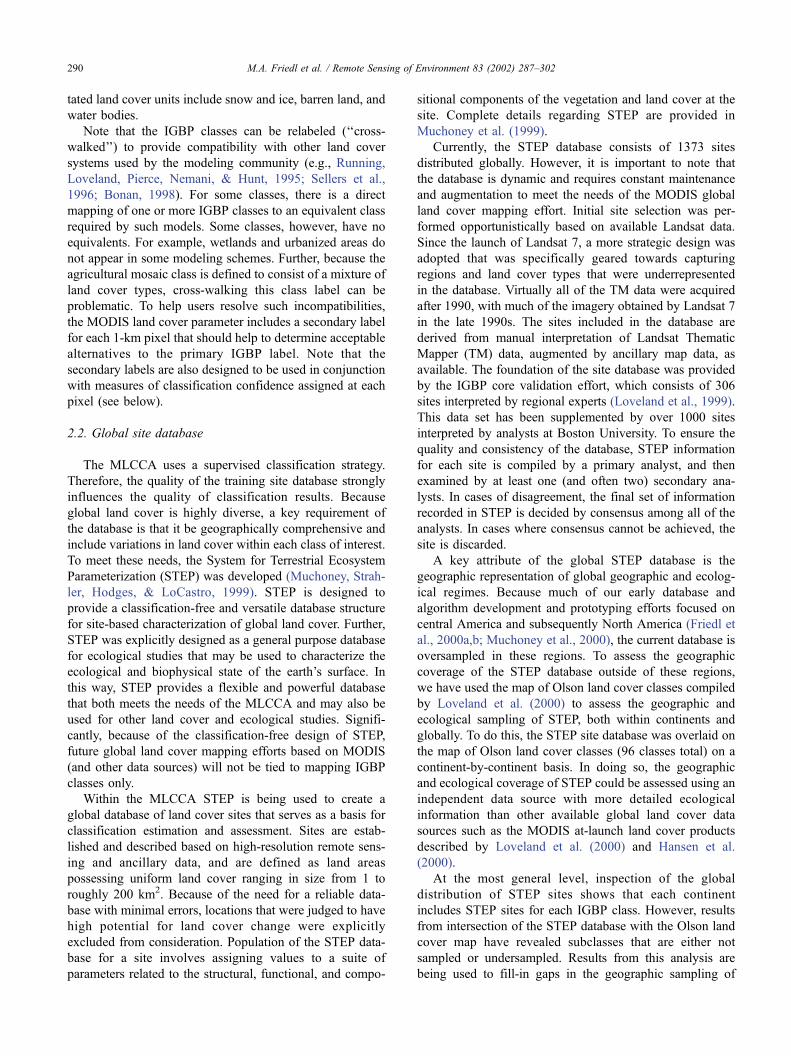
tated land cover units include snow and ice, barren land, and

water bodies.

Note that the IGBP classes can be relabeled (‘‘cross-

walked’’) to provide compatibility with other land cover

systems used by the modeling community (e.g., Running,

Loveland, Pierce, Nemani, & Hunt, 1995; Sellers et al.,

1996; Bonan, 1998). For some classes, there is a direct

mapping of one or more IGBP classes to an equivalent class

required by such models. Some classes, however, have no

equivalents. For example, wetlands and urbanized areas do

not appear in some modeling schemes. Further, because the

agricultural mosaic class is defined to consist of a mixture of

land cover types, cross-walking this class label can be

problematic. To help users resolve such incompatibilities,

the MODIS land cover parameter includes a secondary label

for each 1-km pixel that should help to determine acceptable

alternatives to the primary IGBP label. Note that the

secondary labels are also designed to be used in conjunction

with measures of classification confidence assigned at each

pixel (see below).

2.2. Global site database

The MLCCA uses a supervised classification strategy.

Therefore, the quality of the training site database strongly

influences the quality of classification results. Because

global land cover is highly diverse, a key requirement of

the database is that it be geographically comprehensive and

include variations in land cover within each class of interest.

To meet these needs, the System for Terrestrial Ecosystem

Parameterization (STEP) was developed (Muchoney, Strah-

ler, Hodges, & LoCastro, 1999). STEP is designed to

provide a classification-free and versatile database structure

for site-based characterization of global land cover. Further,

STEP was explicitly designed as a general purpose database

for ecological studies that may be used to characterize the

ecological and biophysical state of the earth’s surface. In

this way, STEP provides a flexible and powerful database

that both meets the needs of the MLCCA and may also be

used for other land cover and ecological studies. Signifi-

cantly, because of the classification-free design of STEP,

future global land cover mapping efforts based on MODIS

(and other data sources) will not be tied to mapping IGBP

classes only.

Within the MLCCA STEP is being used to create a

global database of land cover sites that serves as a basis for

classification estimation and assessment. Sites are estab-

lished and described based on high-resolution remote sens-

ing and ancillary data, and are defined as land areas

possessing uniform land cover ranging in size from 1 to

roughly 200 km2. Because of the need for a reliable data-

base with minimal errors, locations that were judged to have

high potential for land cover change were explicitly

excluded from consideration. Population of the STEP data-

base for a site involves assigning values to a suite of

parameters related to the structural, functional, and compo-

sitional components of the vegetation and land cover at the

site. Complete details regarding STEP are provided in

Muchoney et al. (1999).

Currently, the STEP database consists of 1373 sites

distributed globally. However, it is important to note that

the database is dynamic and requires constant maintenance

and augmentation to meet the needs of the MODIS global

land cover mapping effort. Initial site selection was per-

formed opportunistically based on available Landsat data.

Since the launch of Landsat 7, a more strategic design was

adopted that was specifically geared towards capturing

regions and land cover types that were underrepresented

in the database. Virtually all of the TM data were acquired

after 1990, with much of the imagery obtained by Landsat 7

in the late 1990s. The sites included in the database are

derived from manual interpretation of Landsat Thematic

Mapper (TM) data, augmented by ancillary map data, as

available. The foundation of the site database was provided

by the IGBP core validation effort, which consists of 306

sites interpreted by regional experts (Loveland et al., 1999).

This data set has been supplemented by over 1000 sites

interpreted by analysts at Boston University. To ensure the

quality and consistency of the database, STEP information

for each site is compiled by a primary analyst, and then

examined by at least one (and often two) secondary ana-

lysts. In cases of disagreement, the final set of information

recorded in STEP is decided by consensus among all of the

analysts. In cases where consensus cannot be achieved, the

site is discarded.

A key attribute of the global STEP database is the

geographic representation of global geographic and ecolog-

ical regimes. Because much of our early database and

algorithm development and prototyping efforts focused on

central America and subsequently North America (Friedl et

al., 2000a,b; Muchoney et al., 2000), the current database is

oversampled in these regions. To assess the geographic

coverage of the STEP database outside of these regions,

we have used the map of Olson land cover classes compiled

by Loveland et al. (2000) to assess the geographic and

ecological sampling of STEP, both within continents and

globally. To do this, the STEP site database was overlaid on

the map of Olson land cover classes (96 classes total) on a

continent-by-continent basis. In doing so, the geographic

and ecological coverage of STEP could be assessed using an

independent data source with more detailed ecological

information than other available global land cover data

sources such as the MODIS at-launch land cover products

described by Loveland et al. (2000) and Hansen et al.

(2000).

At the most general level, inspection of the global

distribution of STEP sites shows that each continent

includes STEP sites for each IGBP class. However, results

from intersection of the STEP database with the Olson land

cover map have revealed subclasses that are either not

sampled or undersampled. Results from this analysis are

being used to fill-in gaps in the geographic sampling of


STEP within each of the major continents. To illustrate, Fig.

1 shows results from this analysis for Africa and demon-

strates that by and large, the STEP database is inclusive of

the large majority of Olson land cover classes for this

landmass. Eight Olson classes (out of 36 total) were not

captured by the STEP database, all of which belong to

agricultural classes. Fig. 1 shows the location of TM scenes

that have been targeted to fill in these gaps. Note that this

analysis considers ecological and geographic coverage only,

and does not include consideration of within-class variation.

Fig. 1. STEP sampling of Olson classes in Africa. The red flags show the distribution of sites and the colored areas show Olson classes not sampled by the

STEP database. Candidate TM scenes to fill in gaps are also shown.


However, to a first order, the results from this exercise show

that the STEP database includes relatively good coverage

within Africa. These results are representative of the other

continents, with the exception of Eurasia, which is charac-

terized by complex vegetation and land cover, and which is

the focus of ongoing STEP database development.

2.3. Algorithm inputs

Table 2 presents the list of inputs provided to the

MLCCA. These inputs (features) are designed to exploit

all available information dimensions from MODIS. In par-

ticular, spectral, temporal, directional, and spatial informa-

tion are all included as part of the feature space provided to

the algorithm. At present, the two main information dimen-

sions being used are the spectral and temporal domains.

Spectral information is provided by the seven MODIS land

bands (channels 1–7), and by the enhanced vegetation index

(EVI) product, which provides a measure of the amount and

fractional cover of live vegetation within each 1-km pixel

(Huete & Liu, 1994). Both the reflectance and EVI data are

cloud-cleared and atmospherically corrected, and are

designed to be representative for 16-day periods.

As we alluded to above, the spectral, radiometric, and

geometric quality of MODIS data provides a significant

improvement in the input feature space relative to the

heritage AVHRR data previously used for global land cover

mapping. While significant correlation is present among the

MODIS land bands, spectral information provided by the

MODIS short-wave infrared bands affords at least one

additional dimension of information relative to the red and

near infrared bands provided by AVHRR data (see for

example Crist & Cicone, 1984). Further, the sub-pixel

geometric registration of MODIS data in combination with

superior calibration, cloud screening, and atmospheric cor-

rection provides a substantially improved basis for land

cover mapping relative to AVHRR data. Finally, because the

MODIS instrument views the earth’s surface from a range of

view zenith angles, the MLCCA uses nadir BRDF-adjusted

reflectance (NBAR) data based on the MODIS BRDF/

albedo product (Lucht, Schaaf, & Strahler, 2000). By using

NBAR data, a substantial source of noise (i.e., directional

reflectance effects unrelated to land cover) is removed from

the input data.

To exploit temporal information related to vegetation

phenology, the algorithm is designed to ingest 12 months

of 16-day NBAR and EVI data. Once a full year of

consistently calibrated data is available, phenological met-

rics (e.g., Reed et al., 1994) derived from the EVI will also

be included as inputs. In the longer term, we anticipate

exploiting directional information derived from the MODIS

BRDF/albedo product, and spatial texture information

derived from the MODIS 250-m bands. The former should

provide information related to land cover structure, while

the latter will provide information on sub-kilometer scale

land cover heterogeneity. At present, however, the MLCCA

relies exclusively on spectral and temporal information.

2.4. Classification algorithms

To provide robust and repeatable maps of global land

cover at quarterly time steps, the MLCCA requires classi-

fication algorithms that are capable of efficiently processing

large volumes of complex and high-dimensional data. To

meet these needs, the classification algorithms used by the

MODIS land cover product employ a supervised method-

ology.

Two main classification algorithms have been exten-

sively tested for use within the MLCCA processing flow:

a univariate decision tree (C4.5; Quinlan, 1993) and an

artificial neural network (ARTMAP; Carpenter, Grossberg,

Markuzon, Reynolds, & Rosen, 1992). Both C4.5 and

ARTMAP are distribution-independent and make no

assumptions regarding the underlying frequency distribution

of the data being classified. This attribute is particularly

important at global scales because virtually all classes of

interest exhibit multimodal frequency distributions and,

therefore, violate assumptions required by traditional super-

vised approaches such as the maximum likelihood classifier.

An excellent example of this property is illustrated by

semiarid systems such as grasslands, which are globally

extensive and sensitive to precipitation timing and amount

(Goward & Prince, 1995). This sensitivity leads to distinct

spectral-temporal patterns (subclasses) within the highly

Table 2

The input features used by the MODIS land cover classification algorithm

Input Source Description Time step

Surface reflectancea MODIS reflectance BRDF-adjusted, 7-channel nadir reflectance 16-day

Vegetation indexa MODIS VI EVI index 16-day

BRDF MODIS BRDF shape information 16-day

Land/watera USGS land/sea mask initially (eventually based

on previous quarterly MODIS land cover)

terrestrial/marine boundary fixed

Snow/ice cover MODIS snow/ice snow and ice 16-day

Surface temperature MODIS surface temp. maximum 16-day

Texture MODIS reflectance maximum texture based on 250m channel 1 16-day

Topography USGS DEM slope aspect, slope gradient, elevation fixed

a Used in early results presented in this paper.


generalized classes defined by the IGBP system that must be

accommodated by the MLCCA.

For a variety of mostly practical reasons, the MLCCA

has adopted C4.5 as the primary classification algorithm

used in the generation of global land cover maps. As we

discuss below, missing data caused by cloud cover and

incomplete coverage of NBAR data present a key technical

challenge to the MLCCA. In this regard, C4.5 includes

mature and robust procedures for handling missing data

(Quinlan, 1993). Similar methods for ARTMAP are cur-

rently in development, but are not sufficiently mature at this

time for inclusion in operational code. As a result, C4.5 is

being used because of efficiency considerations and because

of its ability to handle missing data. Friedl, Brodley, and

Strahler (1999), Friedl et al. (2000a,b) and Gopal, Wood-

cock, and Strahler (1999) provide details regarding the

evaluation and testing of C4.5 and ARTMAP for the

MLCCA.

A key feature of the MLCCA is a technique known as

‘‘boosting’’ (Freund, 1995). Boosting is one of numerous

ensemble classification methods that were developed in the

mid- to late 1990s that have been widely shown to enhance

classification accuracy (Bauer & Kohavi, 1999; Dietterich,

2000). Boosting also serves to minimize the sensitivity of

the classification algorithm to noise in feature data and

labeling errors in training data. While many forms of

ensemble algorithms have been developed, most use iter-

ative methods where multiple classifications are estimated

based on resampled versions of the training data. The final

classification for each case is then produced by a weighted

vote. Indeed, Friedman, Hastie, and Tibshirani (2000)

recently described boosting as ‘‘one of the most important

recent developments in classification methodology.’’ While

most of the development work for boosting has been

performed in the machine learning community, recent work

has confirmed that boosting is effective for remote sensing-

based land cover mapping (Friedl et al., 1999; McIver &

Friedl, 2001). It is important to note that boosting is not

effective in the presence of excessive error in training

labels, or if the base classification algorithm (e.g., a decision

tree) does not provide classification accuracy greater than

50%. To minimize problems associated with the former

issue, substantial efforts have been devoted to quality assur-

ance of the STEP site database, and the latter issue does not

apply.

An additional (and perhaps more important) attribute of

boosting arises from recent work by Friedman et al. (2000),

who demonstrated that boosting is equivalent to a form of

additive logistic regression. Prior to this development,

boosting was largely viewed as a black box, albeit a very

successful one. The work of Friedman et al. (2000) provides

a major step forward because it explains this technique

using well-established statistical theory. By using boosting

in association with a base classification algorithm (e.g.,

C4.5), probabilities of class membership can be assigned

to each class at every pixel. Using this approach, we have

developed methods to (1) assign classification confidence

at each pixel and (2) correct major errors based on ancillary

data encoded in the form of prior probabilities (McIver &

Friedl, 2002). In Section 3, we provide further details and

examples regarding the use of boosting within the

MLCCA.

2.5. Validation and assessment

Validation and assessment of classification results is a

key component of the MLCCA, and a variety of approaches

are being pursued to both quantify the quality of land cover

maps produced from MODIS data and assess specific

weaknesses. These approaches include both formal statisti-

cal assessment methods and less formal qualitative assess-

ments.

To provide quantitative estimates of map accuracy, cross-

validation methods will be used to estimate overall and class

specific accuracies at both global and continental scales. In

addition, estimates of classification confidence are assigned

to each pixel based on information extracted from the results

of boosting (see below). To avoid biased results arising from

nonindependent test data at the scale of pixels within

individual sites, cross-validation methods are used that

enforce spatial separation of training and testing data. This

type of procedure is necessary because at 1-km spatial

resolution, MODIS data exhibits considerable spatial auto-

correlation at the scale of individual sites. As a result, cross-

validation procedures that utilize random splits of site data

must ensure that the test data are independent from the test

data, and failure to impose this condition can result in

spuriously inflated classification accuracies (e.g., Friedl et

al., 2000b). Less formally, we have developed collabora-

tions with international groups to provide us with feedback

regarding the quality of the MODIS global land cover

product at local and regional scales. While such feedback

cannot be quantified in the same way as a formal statistical

assessment, this type of information is an invaluable

resource for improving our maps.

In the long run, validation of the MODIS global land

cover product will require a carefully designed probability-

based sample design. This type of approach is the only

means of providing objective and statistically defensible

accuracy statistics (Stehman, 2001). Unfortunately, current

resources do not provide for this type of effort, and so for

the short term, validation efforts will rely on the more

opportunistic strategies described above.

3. Early results

The algorithm theoretical basis document for the MODIS

land cover parameter provides for a release date 15 months

after the launch of Terra (Strahler et al., 1999). The basis for

this timing was to provide a full year’s worth of data for

classification, and to allow several months for resolving


unforeseen problems in data processing. The results pre-

sented below are based on nine 16-day periods spanning the

period from July 11 to December 17, 2000 (note, data were

unavailable from July 27 to August 11 due to problems in

ground processing). These composites represent all avail-

able data of acceptable quality at the time of this writing and

provided the basis of the first official (‘‘beta’’) release of the

MODIS land cover product on April 13, 2001. Note that

because this data set does not include a full annual cycle, the

MLCCA is missing a key dimension of the input feature

space that it is explicitly designed to exploit (i.e., vegetation

phenology). Also, because of cloud cover and data process-

ing issues many pixels possess significantly fewer than nine

views. Fig. 2 presents histograms for the number of views

available at each land pixel globally and for each of the

earth’s major landmasses, and illustrates the degree to which

data are missing for large areas of the earth’s surface.

For the results presented below, classifications were only

performed for those pixels where three or more views were

available. Despite the limited data set available, initial

results from the MLCCA are encouraging and conclusively

demonstrate the quality of MODIS data for land cover

mapping applications. In particular, the quality of the early

results strongly supports the assertion that the spectral

information content of MODIS provides a sound basis for

large-scale land cover mapping.

3.1. Global and regional results

Fig. 3 presents a global classification using the limited

input data described above. At the scale presented, it is

difficult to assess the quality of the MLCCA results in any

concrete way. Nonetheless, the global distribution of land

cover as depicted in Fig. 3 appears to be realistic, and the

coarse scale distribution of natural vegetation is in good

agreement with the expected distribution of forests (and the

IGBP subtypes thereof), shrublands, savannas, and grass-

lands. Further, the agricultural belts of North America,

South America, and Europe are all well characterized, at

least qualitatively. At the same time, some obvious prob-

Fig. 2. Histogram showing the relative frequency distribution for the number of views per pixel provided as input to the classification for each continent, and

for the earth as a whole.


Fig. 3. Early result from MODIS showing the global map of land cover based on the IGBP classification. Missing data is portrayed in black.

M.A.Fried

let

al./Rem

ote

Sensin

gofEnviro

nment83(2002)287–302

295

lems are evident. In particular, the quality of the map

decreases at higher latitudes (>70j) because of missing data

and lower data quality caused by low solar zenith angles,

and confusion is present between agriculture and natural

vegetation throughout. Operationally, the MLCCA uses land

cover values from the previous quarter to fill-in values

where the classification for the current quarter fails. In this

case, the EDC IGBP map is used for this purpose, and

represents about 10% of the land pixels, mostly in the

tropics. Once a 12-month cycle of observations is available,

these cases should be somewhat rare.

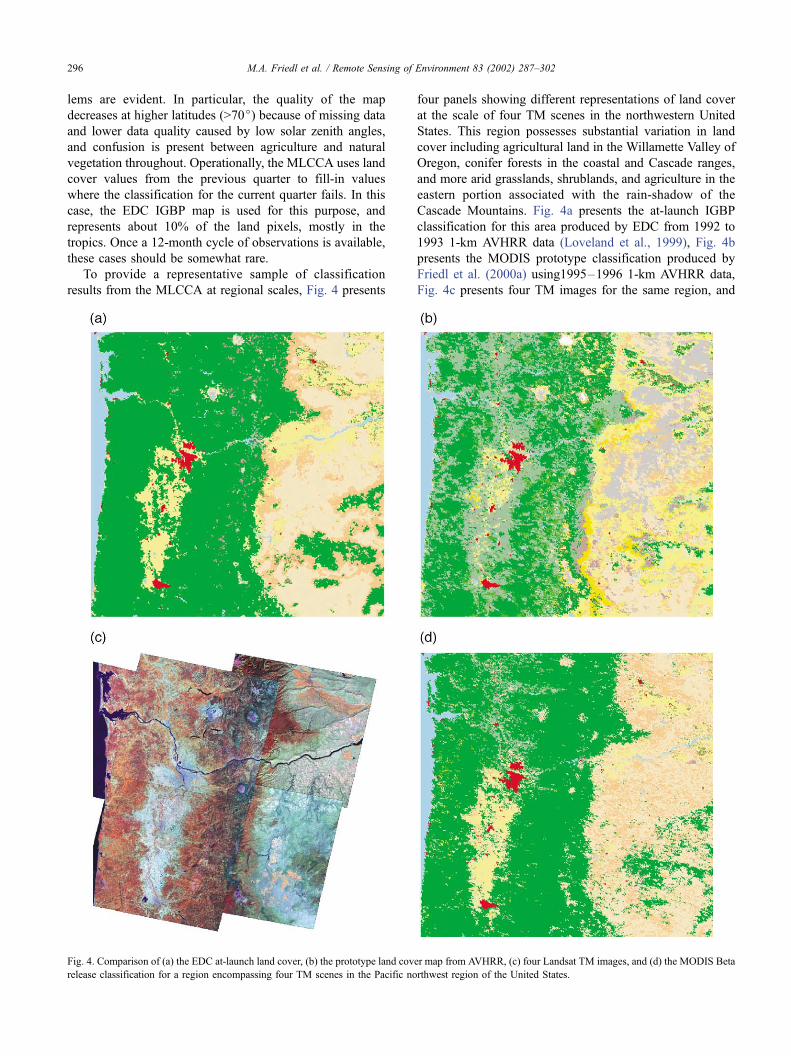
To provide a representative sample of classification

results from the MLCCA at regional scales, Fig. 4 presents

four panels showing different representations of land cover

at the scale of four TM scenes in the northwestern United

States. This region possesses substantial variation in land

cover including agricultural land in the Willamette Valley of

Oregon, conifer forests in the coastal and Cascade ranges,

and more arid grasslands, shrublands, and agriculture in the

eastern portion associated with the rain-shadow of the

Cascade Mountains. Fig. 4a presents the at-launch IGBP

classification for this area produced by EDC from 1992 to

1993 1-km AVHRR data (Loveland et al., 1999), Fig. 4b

presents the MODIS prototype classification produced by

Friedl et al. (2000a) using1995–1996 1-km AVHRR data,

Fig. 4c presents four TM images for the same region, and

Fig. 4. Comparison of (a) the EDC at-launch land cover, (b) the prototype land cover map from AVHRR, (c) four Landsat TM images, and (d) the MODIS Beta

release classification for a region encompassing four TM scenes in the Pacific northwest region of the United States.


Fig. 4d presents results from the MLCCA for MODIS data

from July to December 2000.

Visual inspection shows substantial differences among

these different depictions of land cover. One obvious

observation is that the MODIS-based classification provides

more spatial detail than the EDC IGBP map, particularly in

the forested areas and in the arid eastern areas. Further,

comparison of the supervised classifications based on

AVHRR and MODIS data (Fig. 4b and d) exhibits distinct

differences within this area. Because the training site data

used to generate both these maps is the same, most of these

differences arise from the improved spectral and radiometric

quality of MODIS data relative to AVHRR data.

3.2. Exploiting boosting: classification confidence and prior

probabilities

As we indicated above, boosting is used extensively

within the MLCCA. Specifically, the statistical interpreta-

tion of boosting provided by Friedman et al. (2000) allows

robust estimates of per pixel probabilities of class member-

ship to be assigned to each class at each pixel. This

methodology has been previously used with maximum

likelihood classification techniques that assume Gaussian

density functions for the underlying data (e.g., Foody,

Campbell, Todd, & Wood, 1992). For non-Gaussian data,

probability estimates of class membership can be estimated

directly from decision trees or neural networks (for example,

based on the frequency distribution of examples in the leaf

nodes of a decision tree), but such estimates are generally

quite crude (Friedman et al., 2000). The interpretation of

boosting provided by Friedman et al. allows these estimates

to be made with substantially more statistical rigor and

robustness. Within the MLCCA, we have exploited this for

two main purposes: (1) to provide per pixel estimates of

classification confidence (McIver & Friedl, 2002); and (2)

to include ancillary information to help resolve confusion

between classes that have equivocal spectral separability,

especially agriculture and natural vegetation, at global scales

(McIver & Friedl, 2002). This technique also allows the

MLCCA to provide a secondary label (the second most

likely class) to pixels where the confidence in the primary

label is not high.

Fig. 5 presents three panels showing (a) the classification

confidence assigned to the IGBP label at each pixel, (b) the

secondary label provided by the MLCCA for the area shown

in Fig. 4, and (c) the frequency distribution of estimated

confidence in the primary label. The confidence at each pixel

corresponds to the conditional probability assigned to the

primary class label using boosting. To portray this informa-

Fig. 5. (a) Map of per pixel confidences derived from boosting for the area shown in Fig. 4; (b) the secondary label for each pixel in the same region; and

(c) the histogram of classification confidences. Note that pixels for which the assigned primary label is unequivocal (high confidence) are not assigned a

secondary label.


tion while retaining information related to the spatial dis-

tribution of classes, the confidence is represented by the

degree of color saturation at each pixel (Fig. 5a). For the sake

of illustration, the forest, shrubland, and savanna subclasses

have been combined to avoid confusion between variation in

classes versus variation in classification confidence (hue

versus saturation, respectively).

Fig. 5a and b shows that substantial spatial variance is

present in the estimated confidences, which range from 40%

to 100%. Previously, McIver and Friedl (2002) have shown

that the mean classification confidence within a region

predicted by boosting provides a good estimate of the

expected classification accuracy. This suggests that the

approximate accuracy of the MLCCA for the area shown

in Fig. 4 is 75%. As the number of views increases to

include a full year of data, the classification confidences

(and map accuracy) should increase accordingly. Finally,

Fig. 5c shows the map of secondary class labels provided by

Fig. 5 (continued ).


the MLCCA for the same area. This map reveals that the

secondary labels exhibit spatially coherent and reasonable

patterns relative to the primary map labels. For example,

common secondary labels associated with shrublands are

agriculture and grasslands.

In Fig. 6, we present results that illustrate how ancillary

information encoded in the form of prior probabilities has

been used in the MLCCA to correct large-scale confusion

between problematic classes. In particular, agriculture is

both globally extensive and highly variable in terms of its

spectral and temporal properties. Indeed, Loveland et al.

(1999) and Hansen et al. (2000) both indicate that agricul-

ture is by far the most problematic class in global land cover

mapping contexts. To address this issue, McIver and Friedl

(2002) used the maps compiled by Ramankutty and Foley

(1998) depicting the global distribution and intensity of

agriculture to resolve obvious confusion between agriculture

and other land cover types in an AVHRR-based classifica-

tion of North America.

To include this approach within the MLCCA, the maps

of Ramankutty and Foley (1998) and Loveland et al. (2000)

were used to parameterize the prior probability for IGBP

classes globally. To do this, Bayes’ rule was used where the

conditional probabilities of class membership at each pixel

were estimated using boosting. The prior probability for the

presence of agriculture was scaled from 0.1 to 1.0 based on

the estimates of agricultural intensity provided by Raman-

kutty and Foley (1998), and the prior probabilities for other

IGBP classes were estimated from 200� 200 km moving

windows using the EDC at-launch IGBP map. This proce-

dure uses a parameter (c), scaled from 0 to 1.0, which

constrains the influence of the prior probabilities contingent

on the relative quality of the ancillary data (Chen, Ibrahim,

& Yianoutsos, 1999). McIver and Friedl (2002) suggest that

Fig. 6. Map showing classification changes arising from inclusion of prior probabilities for agriculture (yellow= change from agriculture to natural vegetation;

green = change from natural vegetation to agriculture; black = no change.)


a simple way to select a value for this parameter is to use the

accuracy of the ancillary map data (i.e., if the map accuracy

of the ancillary data is 79%, c = 0.79).

Because of the way that boosting estimates per pixel class

membership probabilities, the effect of including prior prob-

abilities in this fashion is fairly conservative. In other words,

the influence of the prior information is restricted to cases

where the spectral classification is ambiguous (i.e., poor

spectral-temporal separability among two or more classes)

and the ancillary information is unequivocal. Further, in

cases where the classes are separable in the input feature

space, the ancillary information has little or no effect. Fig. 6

presents a map showing the pixels that changed from natural

vegetation to agriculture (and vice versa), again for the area

shown in Fig. 4, as a result of including ancillary information

related to the distribution of agriculture. In total, the use of

prior probabilities resulted in 23.3% of the pixels in this

region changing from agriculture to natural vegetation, while

0.7% changed from natural vegetation to agriculture.

These results reflect the fact that the semiarid natural

vegetation in the rain shadow of the Cascade Mountains

possesses spectral-temporal signatures in the MODIS data

that are similar to agriculture. Thus, inclusion of ancillary

information related to the intensity of agricultural land use

helped to reduce overestimation of agriculture in this region.

Once a full year of MODIS data is available, the influence

of the ancillary data should become smaller. Note that the

similarity in spectral-temporal signatures between agricul-

ture and natural vegetation in this region is also reflected in

the secondary labels shown in Fig. 5c. Indeed, this problem

is evident in the AVHRR-based prototype classification for

this region shown in Fig. 4b. While quantitative assessment

regarding the success of this procedure has not yet been

performed, the results seem to be qualitatively reasonable

and are consistent with the distribution of agriculture in the

EDC IGBP map for this region.

4. Discussion and conclusions

This paper describes the databases and methods being

used to create the MODIS land cover product and has

presented early results from applying the MLCCA to 5

months of MODIS data. The classification strategy of the

MLCCA follows a supervised approach. To exploit the best

available classification technology and to avoid assumptions

related to the distribution of input data, the MLCCA uses a

decision tree classification approach. Decision tree techni-

ques previously have been shown to be effective for global

land cover mapping problems. However, they are also

highly sensitive to the training data used in the classification

estimation stage. Therefore, classification results produced

from MODIS data are heavily dependent on the integrity

and representation of global land cover in the site data, and

substantial ongoing efforts are devoted to maintaining and

augmenting the STEP database.

Despite significant data limitations due to cloud cover

and other processing problems, initial results based on 5

months of MODIS data are promising. The quality of early

maps produced from MODIS is especially encouraging

because one of the key information domains (i.e., the

temporal domain) that the MLCCA is designed to exploit

was incomplete. The quality of the early results presented in

this paper, therefore, provides strong evidence supporting

the radiometric quality and spectral information content of

MODIS data for large-scale land cover mapping applica-

tions. MODIS data clearly provides a significant improve-

ment in terms of quality relative to the heritage AVHRR

data, and once a full year of well-calibrated data is available,

we expect that the quality of the global land cover product

will improve accordingly.

The MODIS land cover product utilizes the IGBP clas-

sification system. This system was initially selected to

reflect the consensus representation for land cover desired

by global models in the early to mid-1990s. In the last few

years, it has become increasingly apparent that the frame-

work provided by the IGBP scheme is limited. While IGBP

classes can be cross-walked to other systems, cross-walking

is often problematic, and the 17 classes provided within the

IGBP scheme do not provide a universally acceptable basis

for the diverse community of modeling and land resource

scientists who might otherwise wish to exploit land cover

data sets derived from MODIS.

Because the STEP database is explicitly designed to be

classification-free, we have considerable flexibility in terms

of the land cover products that may be produced from

MODIS data. As a starting point, we are planning to provide

global maps of the six-biome classification system described

by Running et al. (1995), the 14-class classification system

developed at the University of Maryland (DeFries et al.,

1998), and the six-biome classification system described by

Myneni, Nemani, and Running (1997) for radiative transfer

and LAI/FPAR retrievals (see Lotsch, Tian, Friedl, &

Myneni, 2002). In the longer term, we hope to provide a

hierarchical database structure where simplified land cover

and vegetation attributes (e.g., vegetated versus nonvege-

tated; life form; leaf type; etc.) are stored in separate inter-

nally consistent layers. In this way, users can choose to use

the IGBP or other available classification maps, or create

their own classifications based on the data layers provided.

Acknowledgements

This work was supported by NASA contract NAS5-

31369 and NASA Grant NAG5-7218.

References

Bauer, E., & Kohavi, R. (1999). An empirical comparison of voting clas-

sification algorithms: bagging, boosting, and variants. Machine Learn-

ing, 36, 105–139.


Bonan, G. B. (1998). The land surface climatology of the NCAR Land

Surface Model coupled to the NCAR Community Climate Model. Jour-

nal of Climate, 11(6), 1307–1326.

Carpenter, G. A., Grossberg, S., Markuzon, N., Reynolds, J. H., & Rosen,

D. B. (1992). Fuzzy ART: a neural network architecture for incremental

supervised learning of analog multidimensional maps. IEEE Transac-

tions on Neural Networks, 3, 698–713.

Chen, M. H., Ibrahim, J. G., & Yianoutsos, C. (1999). Prior elicitation,

variable selection, and Bayesian computation for logistic regression

models. Journal of the Royal Statistical Society. Series B, Statistical

Methodology, 61, 223–242.

Crist, E. P., & Cicone, R. C. (1984). Application of the tasseled cap concept

to simulated thematic mapper data. Photogrammetric Engineering and

Remote Sensing, 50(3), 343–352.

DeFries, R., Hansen, M., Townsend, J. G. R., & Sohlberg, R. (1998).

Global land cover classifications at 8 km resolution: the use of training

data derived from Landsat imagery in decision tree classifiers. Interna-

tional Journal of Remote Sensing, 19, 3141–3168.

DeFries, R. S., & Townshend, J. G. R. (1994). NDVI derived land cover

classifications at a global scale. International Journal of Remote Sens-

ing, 5, 3567–3586.

Dietterich, T. G. (2000). An experimental comparison of three methods for

constructing ensembles of decision trees: bagging, boosting, and ran-

domization. Machine Learning, 40(2), 139–158.

Foody, G. M., Campbell, N. A., Todd, N. M., & Wood, T. F. (1992).

Derivation and application of class membership from the maximum

likelihood classification. Photogrammetric Engineering and Remote

Sensing, 17, 1389–1398.

Freund, Y. (1995). Boosting a weak learning algorithm by majority. Infor-

mation and Computation, 121(2), 256–285.

Friedl, M. A., Brodley, C. E., & Strahler, A. H. (1999). Maximizing land

cover classification accuracies produced by decision trees at continental

to global scales. IEEE Transactions on Geoscience and Remote Sens-

ing, 37(2), 969–977.

Friedl, M. A., Muchoney, D., McIver, D. K., Gao, F., Hodges, J. C. F., &

Strahler, A. H. (2000a). Characterization of North American land cover

from NOAA-AVHRR data using the EOS MODIS land cover classifi-

cation algorithm. Geophysical Research Letters, 27(7), 977–980.

Friedl, M. A., Woodcock, C., Gopal, S., Muchoney, D., Strahler, A. H., &

Barker-Schaaf, C. (2000b). A note on procedures used for accuracy

assessment in land cover maps derived from AVHRR data. Interna-

tional Journal of Remote Sensing, 21(5), 1073–1077.

Friedman, J., Hastie, T., & Tibshirani, R. (2000). Additive logistic re-

gression: a statistical view of boosting. The Annals of Statistics (28),

337–374.

Gopal, S., Woodcock, C., & Strahler, A. (1999). Fuzzy ARTMAP classi-

fication of global land cover from the 1 degree AVHRR data set. Re-

mote Sensing of Environment, 67, 23–243.

Goward, S. N., & Prince, S. D. (1995). Transient effects of climate on

vegetation dynamics: satellite observations. Journal of Biogeography,

22(2–3), 549–564.

Hansen, M. C., Defries, R. S., Townshend, J. R. G., & Sohlberg, R.

(2000). Global land cover classification at 1 km spatial resolution using

a classification tree approach. International Journal of Remote Sensing,

21(6–7), 1331–1364.

Huete, A. R., & Liu, H. Q. (1994). An error and sensitivity analysis of the

atmospheric-correcting and soil-correcting variants of the NDVI for the

MODIS-EOS. IEEE Transactions on Geoscience and Remote Sensing,

32(4), 897–905.

Lambin, E. F., & Strahler, A. H. (1994a). Indicators of land-cover change

for change-vector analysis in multitemporal space at coarse spatial

scales. International Journal Remote Sensing, 15, 2099–2119.

Lambin, E. F., & Strahler, A. H. (1994b). Change-vector analysis: a tool to

detect and categorize land-cover change processes using high temporal-

resolution satellite data. Remote Sensing of Environment, 48, 231–244.

Lotsch, A., Tian, Y., Friedl, M. A., & Myneni, R. B. (2002). Land cover

mapping in support of LAI/FAPA retrievals from EOS MODIS and

MISR: classification methods and sensitivities to errors. (In review)

International Journal of Remote Sensing.

Loveland, T. R., & Belward, A. S. (1997). The IGBP-DIS global 1-km land

cover data set, DIScover: first results. International Journal of Remote

Sensing, 65(9), 1021–1031.

Loveland, T. R., Reed, B. C., Brown, J. F., Ohlen, D. O., Zhu, Z., Yang, L.,

& Merchant, J. W. (2000). Development of a global land cover charac-

teristics database and IGBP DISCover from 1 km AVHRR data. Inter-

national Journal of Remote Sensing, 21(6–7), 1303–1365.

Loveland, T. R., Zhu, Z., Ohlen, D. O., Brown, J. F., Reed, B. C., & Yang,

L. (1999). An analysis of the IGBP global land cover characterization

process. Photogrammetric Engineering and Remote Sensing, 65(9),

1021–1031.

Lucht, W., Schaaf, C. B., & Strahler, A. H. (2000). An algorithm for the

retrieval of albedo from space using semiempirical BRDF models. IEEE

Transaction on Geoscience and Remote Sensing, 38, 977–998.

Matthews, E. (1983). Global vegetation and land-use: new-high resolution

data bases for climate studies. Journal of Climate and Applied Meteor-

ology, 22, 474–487.

McIver, D. K., & Friedl, M. A. (2001). Estimating pixel-scale land cover

classification confidence using non-parametric machine learning meth-

ods. IEEE Transactions on Geoscience and Remote Sensing, 39(9),

1959–1968.

McIver, D. K., & Friedl, M. A. (2002). Using prior probabilities in deci-

sion tree classification of remotely sensed data. Remote Sensing of

Environment, 81, 253–261.

Muchoney, D., Borak, J., Chi, H., Friedl, M., Gopal, S., Hodges, J., Morrow,

N., & Strahler, A. (2000). Application of the MODIS global supervised

classification model to vegetation and land cover mapping of central

America. International JournalofRemoteSensing,21(6–7), 1115–1138.

Muchoney, D., Strahler, A., Hodges, J., & LoCastro, J. (1999). The IGBP

DISCover confidence sites and the system for terrestrial ecosystem

parameterization: tools for validating global land-cover data. Photo-

grammetric Engineering and Remote Sensing, 65(9), 1061–1067.

Myneni, R. B., Nemani, R. R., & Running, S.W. (1997). Estimation of global

leaf area index and absorbed par using radiative transfer models. IEEE

Transactions on Geoscience and Remote Sensing, 35(6), 1380–1393.

Olson, J. S., & Watts, J. (1982). Major world ecosystem complexes. In D.

B. Jones (Ed.), Earth’s vegetation and atmospheric carbon dioxide.

Carbon dioxide review (pp. 388–399). Oxford: Oxford Univ. Press.

Quinlan, J. R. (1993). C4.5: programs for machine learning. San Mateo,

CA: Morgan Kaufmann.

Ramankutty, N., & Foley, J. A. (1998). Characterizing patterns of global

land use: an analysis of global crop yield data. Global Biogeochemical

Cycles, 12(4), 667–685.

Reed, B. C., Brown, J. F., VanderZee, D., Loveland, T. R., Merchant, J. W.,

& Ohlen, D. O. (1994). Measuring phenological variability from satel-

lite data. Journal of Vegetation Science, 5, 703–714.

Running, S. W., Loveland, T. R., Pierce, L. L., Nemani, R., & Hunt Jr., E. R.

(1995). A remote sensing-based classification logic for global land cover

analysis. Remote Sensing of Environment, 51(1), 39–48.

Schowengerdt, R. A. (1997). Remote sensing models and methods for

image processing. (2nd ed.). San Diego: Academic Press.

Sellers, P. J., Dickinson, R. E., Randall, D. A., Betts, A. K., Hall, F. G.,

Berry, J. A., Collatz, G. J., Denning, A. S., Mooney, H. A., Nobre,

C. A., Sato, N., Field, C. B., & Henderson-Sellers, A. (1997). Modeling

the exchanges of energy, water, and carbon between continents and the

atmosphere. Science, 275(5299), 502–509.

Sellers, P. J., Randall, D. A., Collatz, G. J., Berry, J. A., Field, C. B.,

Dazlich, D. A., Zhang, C., Collelo, G. D., & Bounoua, L. (1996). A

revised land surface parameterization (SiB2) for atmospheric GCMs: 1.

Model formulation. Journal of Climate, 9(4), 676–705.

Stehman, S. V. (2001). Statistical rigor and practical utility in thematic map

accuracy assessment. Photogrammetric Engineering and Remote Sens-

ing, 67(6), 727–734.

Strahler, A., Muchoney, D., Borak, J., Gao, F., Friedl, M., Gopal, S., Hodges,

J., Lambin, E., McIver, D., Moody, A., Schaaf, C., & Woodcock, C.


(1999). MODIS land cover product, algorithm theoretical basis docu-

ment (ATBD), Version 5.0. Boston, MA: Center for Remote Sensing,

Department of Geography, Boston University.

Townshend, J. R. G., Justice, C., Li, W., Gurney, C., & McManus, J.

(1991). Global land cover classification by remote sensing: present

capabilities and future possibilities. Remote Sensing of Environment,

35, 243–255.

Wilson, M., & Henderson-Sellers, A. (1985). A global archive of land cover

and soils data for use in general circulation climate models. Journal of

Climatology, 5, 119–143.


global land cover mapping from modis: algorithms and early results

Documents