cloud retrieval algorithms for modis: optical thickness
TRANSCRIPT

Cloud Retrieval Algorithms for MODIS: Optical Thickness,
Effective Particle Radius, and Thermodynamic Phase
MICHAEL D. KING1 AND SI-CHEE TSAY2
NASA Goddard Space Flight CenterGreenbelt, Maryland 20771
STEVEN E. PLATNICK2 AND MENGHUA WANG3
University of Maryland Baltimore CountyNASA Goddard Space Flight Center
Greenbelt, Maryland 20771
KUO-NAN LIOUDepartment of Atmospheric SciencesUniversity of California Los AngelesLos Angeles,, California 90095-1565
MODIS Algorithm Theoretical Basis Document No. ATBD-MOD-05
MOD06 – Cloud product
(23 December 1997, version 5)
1 Earth Sciences Directorate2 Laboratory for Atmospheres3 Laboratory for Hydrospheric Processes


i
TABLE OF CONTENTS
1. INTRODUCTION....................................................................................................... 1
2. OVERVIEW AND BACKGROUND INFORMATION......................................... 2
2.1. Experimental objectives ..................................................................................... 2
2.2. Historical perspective......................................................................................... 5
2.3. Instrument characteristics.................................................................................. 7
3. ALGORITHM DESCRIPTION ............................................................................... 10
3.1. Theoretical description..................................................................................... 10
3.1.1. Physics of problem ................................................................................. 10
a. Cloud optical thickness and effective particle radius ................. 10
b. Cloud thermodynamic phase ......................................................... 18
c. Ice cloud properties.......................................................................... 20
3.1.2. Mathematical description of algorithm............................................... 22
a. Asymptotic theory for thick layers ................................................ 22
b. Retrieval example............................................................................. 24
c. Atmospheric corrections: Rayleigh scattering............................. 27
d. Atmospheric corrections: Water vapor ........................................ 29
e. Technical outline of multi-band algorithm................................... 30
f. Retrieval of cloud optical thickness and effective radius ........... 36
3.2. Variance and uncertainty estimates............................................................... 41
3.2.1. Model uncertainties................................................................................ 42
3.2.2. Physical uncertainties ............................................................................ 49
3.3. Practical considerations ................................................................................... 53
3.3.1. Numerical computation considerations.............................................. 53

ii
a. Parameter description...................................................................... 53
b. Required input data ......................................................................... 56
c. Data processing path and requirements ....................................... 57
d. Data storage estimates ..................................................................... 58
e. Level-3 gridded data........................................................................ 61
3.3.2. Validation ................................................................................................ 62
3.3.3. Quality control, diagnostics, and exception handling ...................... 68
4. CONSTRAINTS, LIMITATIONS, AND ASSUMPTIONS.................................. 68
5. REFERENCES ........................................................................................................... 69
APPENDIX. ACRONYMS............................................................................................. 77

1
1. Introduction
The intent of this document is to present algorithms for inferring certain op-
tical and thermodynamical properties of cloud layers, specifically, optical thick-
ness, effective particle radius, and particle phase from multiwavelength reflected
solar and emitted thermal radiation measurements.
It is well known that clouds strongly modulate the energy balance of the
Earth and its atmosphere through their interaction with solar and terrestrial ra-
diation, as demonstrated both from satellite observations (Ramanathan 1987,
Ramanathan et al. 1989) and from modeling studies (Ramanathan et al. 1983,
Cess et al. 1989). However, clouds vary considerably in their horizontal and ver-
tical extent (Stowe et al. 1989, Rossow et al. 1989), in part due to the circulation
pattern of the atmosphere with its requisite updrafts and downdrafts, and in part
due to the distribution of oceans and continents and their numerous and varied
sources of cloud condensation nuclei (CCN). A knowledge of cloud properties
and their variation in space and time, therefore, is crucial to studies of global cli-
mate change (e.g., trace gas greenhouse effects), as general circulation model
(GCM) simulations indicate climate-induced changes in cloud amount and verti-
cal structure (Wetherald and Manabe 1988), with a corresponding cloud feedback
working to enhance global warming.
GCM simulations by Roeckner et al. (1987) and Mitchell et al. (1989) include
corresponding changes in cloud water content and optical thickness, and suggest
that changes in cloud optical properties may result in a negative feedback com-
parable in size to the positive feedback associated with changes in cloud cover.
None of the GCM simulations to date include corresponding changes in cloud
microphysical properties (e.g., particle size), which could easily modify conclu-
sions thus far obtained. Of paramount importance to a comprehensive under-

ALGORITHM THEORETICAL BASIS DOCUMENT, OCTOBER 1996 2
standing of the Earth’s climate and its response to anthropogenic and natural
variability is a knowledge, on a global sense, of cloud properties that may be
achieved through remote sensing and retrieval algorithms.
In this document we start with a background overview of the MODIS in-
strumentation and the cloud retrieval algorithms, followed by a description of
the theoretical basis of the cloud retrieval algorithms to be applied to MODIS
data. We follow with a discussion of practical considerations (including the con-
straints and limitations involved in the retrieval algorithms), outline our valida-
tion strategy, and present our plans for refinement of the algorithms during the
pre-launch and post-launch development phases.
2. Overview and background information
The purpose of this document is to provide a description and discussion of
the physical principles and practical considerations behind the remote sensing
and retrieval algorithms for cloud properties that we are developing for MODIS.
Since the development of the algorithms, to be used in analyzing data from the
MODIS sensor system, is at the at-launch software development stage, this
document is based on methods that have previously been developed for proc-
essing data from other sensors with similar spectral characteristics. Through
continued interaction with the MODIS science team and external scientific com-
munity, we anticipate that these algorithms will be further refined for use in the
processing of MODIS data, both through simulations and through airborne field
experiments.
2.1. Experimental objectives
The main objective of this work is the development of routine and opera-
tional methods for simultaneously retrieving the cloud optical thickness and ef-
KING ET AL.: REMOTE SENSING OF CLOUD PROPERTIES FROM MODIS 3
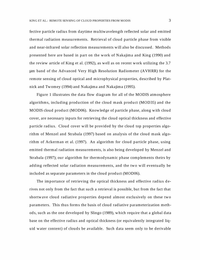
fective particle radius from daytime multiwavelength reflected solar and emitted
thermal radiation measurements. Retrieval of cloud particle phase from visible
and near-infrared solar reflection measurements will also be discussed. Methods
presented here are based in part on the work of Nakajima and King (1990) and
the review article of King et al. (1992), as well as on recent work utilizing the 3.7
µm band of the Advanced Very High Resolution Radiometer (AVHRR) for the
remote sensing of cloud optical and microphysical properties, described by Plat-
nick and Twomey (1994) and Nakajima and Nakajima (1995).
Figure 1 illustrates the data flow diagram for all of the MODIS atmosphere
algorithms, including production of the cloud mask product (MOD35) and the
MODIS cloud product (MOD06). Knowledge of particle phase, along with cloud
cover, are necessary inputs for retrieving the cloud optical thickness and effective
particle radius. Cloud cover will be provided by the cloud top properties algo-
rithm of Menzel and Strabala (1997) based on analysis of the cloud mask algo-
rithm of Ackerman et al. (1997). An algorithm for cloud particle phase, using
emitted thermal radiation measurements, is also being developed by Menzel and
Strabala (1997); our algorithm for thermodynamic phase complements theirs by
adding reflected solar radiation measurements, and the two will eventually be
included as separate parameters in the cloud product (MOD06).
The importance of retrieving the optical thickness and effective radius de-
rives not only from the fact that such a retrieval is possible, but from the fact that
shortwave cloud radiative properties depend almost exclusively on these two
parameters. This thus forms the basis of cloud radiative parameterization meth-
ods, such as the one developed by Slingo (1989), which require that a global data
base on the effective radius and optical thickness (or equivalently integrated liq-
uid water content) of clouds be available. Such data seem only to be derivable

ALGORITHM THEORETICAL BASIS DOCUMENT, OCTOBER 1996 4
from spaceborne remote sensing observations. Therefore, MODIS is ideally
suited to cloud remote sensing applications and retrieval purposes.
9/3/96
Leve
l 1 MOD02Calibrated L1B Radiance
MOD03Geolocation Fields
Leve
l 0
MOD01Level 1A
MOD02 MOD03
Leve
l 2
MOD07Atmospheric Profiles
• Total Ozone Burden• Stability Indices
• Temp & Moisture Profiles• Precipitable Water (IR)
MOD05Precipitable
Water Product
• Solar Algorithm• IR Algorithm
MOD35Cloud Mask
MODIS Atmosphere Processing
MOD04 Aerosol Product
• Aerosol Optical Thickness
• Aerosol Size Distribution
MOD06Cloud Product
• Cloud Top Properties (temperature, height, emissivity)
• Cloud Particle Phase• Cloud Fraction
• Cloud Optical Properties (optical thickness and particle size)
Leve
l 3
MOD03, Level 2 Atmosphere Products
MOD02, MOD03, MOD07, MOD35
MOD11 L2G Land Temp.
MOD21L2 Chlorophyll Conc.
MOD33 Snow Cover(prior period)
MOD43 BRDF/Albedo
(16-day)
MOD08L3 Atmosphere Joint Product:
• Aerosol • Water Vapor• Clouds • Stability Indices• Ozone
(daily, 8-day, monthly)
Instrument Packet Data
Figure 1. Data flow diagram for the MODIS atmosphere products, including productMOD06, some parameters of which (optical thickness and effective particlesize) are produced by the algorithm described in this ATBD-MOD-06.

KING ET AL.: REMOTE SENSING OF CLOUD PROPERTIES FROM MODIS 5
2.2. Historical perspective
Ever since the first launch of the TIROS-1 satellite in 1960, tremendous inter-
est has arisen in the field of using these remotely sensed data to establish a global
cloud climatology, in which a qualitative cloud atlas was archived. It has been a
long-standing goal to quantify global cloud properties from spaceborne observa-
tions, such as cloud cover, cloud particle thermodynamic phase, cloud optical
thickness and effective particle radius, and cloud top altitude and temperature.
Many efforts in the past three decades (e.g., work dated as early as 1964 by Ark-
ing) have been devoted to extracting cloud cover parameters from satellite meas-
urements.
There are a number of studies of the determination of cloud optical thickness
and/or effective particle radius with visible and near-infrared radiometers on
aircraft (Hansen and Pollack 1970, Twomey and Cocks 1982 and 1989, King 1987,
Foot 1988, Rawlins and Foot 1990, Nakajima and King 1990, Nakajima et al. 1991)
and on satellites (Curran and Wu 1982, Rossow et al. 1989). Further, the utility of
the 3.7 µm band onboard the AVHRR has been demonstrated by several investi-
gators, including Arking and Childs (1985), Durkee (1989), Platnick and Twomey
(1994), Han et al. (1994, 1995), Nakajima and Nakajima (1995) and Platnick and
Valero (1995). The underlying principle on which these techniques are based is
the fact that the reflection function of clouds at a nonabsorbing band in the visi-
ble wavelength region is primarily a function of the cloud optical thickness,
whereas the reflection function at a water (or ice) absorbing band in the near-
infrared is primarily a function of cloud particle size.
Twomey and Cocks (1989) developed a statistical method for simultaneously
determining the cloud optical thickness and effective radius using reflected in-
tensity measurements at several wavelengths in the near-infrared region. An

ALGORITHM THEORETICAL BASIS DOCUMENT, OCTOBER 1996 6
extension of this technique addresses the problem of identifying the thermody-
namic phase of clouds (ice vs water) and of distinguishing clouds from snow sur-
faces by utilizing particular bands (e.g., 1.64 and 2.2 µm) which provide different
absorption characteristics of water and ice (e.g., Pilewskie and Twomey 1987).
Although these studies have demonstrated the applicability of remote sens-
ing methods to the determination of cloud optical and microphysical properties,
more theoretical and experimental studies are required in order to assess the
soundness and accuracy of these methods when applied to measurements on a
global scale. From the theoretical point of view, the application of asymptotic
theory to the determination of cloud optical thickness (King 1987) has demon-
strated the physical basis of the optical thickness retrieval and its efficient im-
plementation to experimental observations. This method is worth incorporating
as one component of any multiwavelength algorithm for simultaneously deter-
mining the cloud particle phase, optical thickness and effective particle radius.
From the experimental point of view, more aircraft validation experiments are
required in order to assess the validity of these methods, since many factors af-
fect the successful retrieval of these parameters when applied to real data in a
real atmosphere (e.g., Rossow et al. 1985, Wu 1985).
Since 1986, an extensive series of field observations has been conducted.
These include: FIRE-I/II Cirrus (First ISCCP Regional Experiment, 1986 and
1991, respectively), FIRE-I Stratocumulus (1987), ASTEX (Atlantic Stratocumulus
Transition Experiment, 1992), TOGA/COARE (Tropical Ocean Global Atmos-
phere/Coupled Ocean-Atmosphere Response Experiment, 1993), CEPEX
(Central-Equatorial Pacific Experiment, 1993), SCAR-A (Sulfate, Clouds And Ra-
diation-Atlantic, 1993), MAST (Monterey Area Ship Track Experiment, 1994),
SCAR-C (Smoke, Clouds And Radiation - California, 1994), ARMCAS (Arctic
KING ET AL.: REMOTE SENSING OF CLOUD PROPERTIES FROM MODIS 7
Radiation Measurements in Column Atmosphere-surface System, 1995), SCAR-B
(Smoke, Clouds And Radiation - Brazil, 1995), and SUCCESS (Subsonic Aircraft
Contrail and Cloud Effects Special Study, 1996). Instrumentation involved in
these experiments has included either the MCR (Multispectral Cloud Radiome-
ter; Curran et al. 1981) or MAS (MODIS Airborne Simulator; King et al. 1996),
airborne sensors having spectral characteristics similar to a number of the cloud
retrieval bands contained in MODIS, as well as the NOAA AVHRR satellite sen-
sor. In the pre-launch stage of MODIS, these observational data, especially MAS
data for which more than 500 research hours have thus far been obtained under
various all-sky conditions, form the basis for our cloud retrieval algorithm de-
velopment and validation.
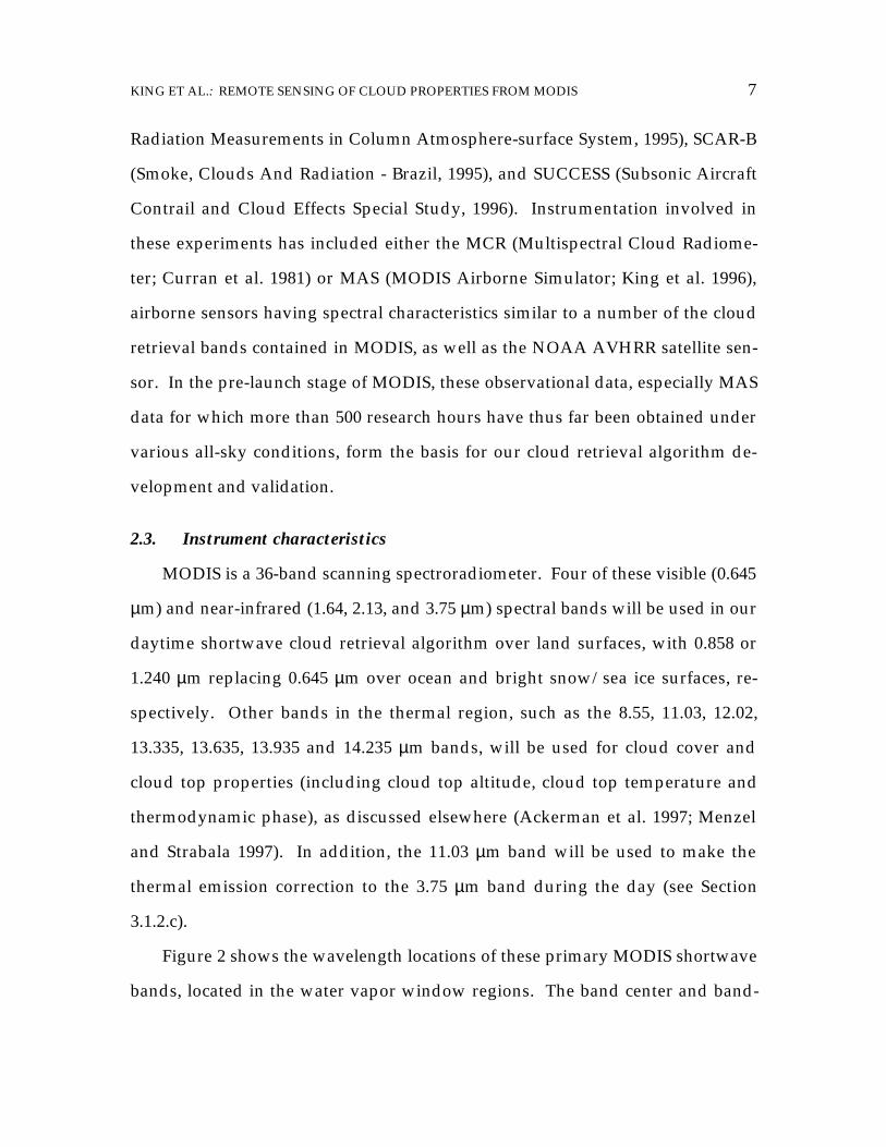
2.3. Instrument characteristics
MODIS is a 36-band scanning spectroradiometer. Four of these visible (0.645
µm) and near-infrared (1.64, 2.13, and 3.75 µm) spectral bands will be used in our
daytime shortwave cloud retrieval algorithm over land surfaces, with 0.858 or
1.240 µm replacing 0.645 µm over ocean and bright snow/sea ice surfaces, re-
spectively. Other bands in the thermal region, such as the 8.55, 11.03, 12.02,
13.335, 13.635, 13.935 and 14.235 µm bands, will be used for cloud cover and
cloud top properties (including cloud top altitude, cloud top temperature and
thermodynamic phase), as discussed elsewhere (Ackerman et al. 1997; Menzel
and Strabala 1997). In addition, the 11.03 µm band will be used to make the
thermal emission correction to the 3.75 µm band during the day (see Section
3.1.2.c).
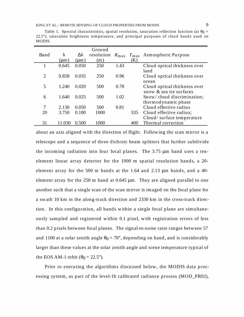
Figure 2 shows the wavelength locations of these primary MODIS shortwave
bands, located in the water vapor window regions. The band center and band-

ALGORITHM THEORETICAL BASIS DOCUMENT, OCTOBER 1996 8
width characteristics, as well as the dynamic range and main purpose(s) of each
band, are also summarized in Table 1. The 0.645, 2.13 and 3.75 µm bands will be
used to retrieve the cloud optical thickness and effective particle radius over land
(with 0.645 µm replaced by 0.858 µm over oceans and 1.24 µm over snow and sea
ice surfaces); a combination of the 0.645, 1.64, and possibly the 2.13 µm bands
will be used for cloud thermodynamic phase determination.
MODIS is designed to scan through nadir in a plane perpendicular to the
velocity vector of the spacecraft, with the maximum scan extending up to 55° on
either side of nadir (110° aperture). At a nominal orbital altitude for the EOS
AM-1 spacecraft of 705 km, this yields a swath width of 2330 km centered on the
satellite ground track. In the baseline concept, the Earth-emitted and reflected
solar radiation is incident on a two-sided scan mirror that continually rotates
θ0 = 10°
0.0
0.2
0.4
0.6
0.8
1.0
0.5 1.0 1.5 2.0 2.5 3.0 3.5 4.0
18 km10 kmSurface
Tra
nsm
ittan
ceMcClatchey Tropical Atmosphere
Wavelength (µm)Figure 2. Spectral characteristics of six MODIS bands, centered at 0.65, 0.86, 1.24, 1.64,
2.13, and 3.75 µm, used for cloud property detection. The atmospheric trans-mittances are calculated from LOWTRAN 7 at 18 km, 10 km and at the surfacefor the McClatchey tropical atmosphere at 10° solar zenith angle.
KING ET AL.: REMOTE SENSING OF CLOUD PROPERTIES FROM MODIS 9
about an axis aligned with the direction of flight. Following the scan mirror is a
telescope and a sequence of three dichroic beam splitters that further subdivide
the incoming radiation into four focal planes. The 3.75 µm band uses a ten-
element linear array detector for the 1000 m spatial resolution bands, a 20-
element array for the 500 m bands at the 1.64 and 2.13 µm bands, and a 40-
element array for the 250 m band at 0.645 µm. They are aligned parallel to one
another such that a single scan of the scan mirror is imaged on the focal plane for
a swath 10 km in the along-track direction and 2330 km in the cross-track direc-
tion. In this configuration, all bands within a single focal plane are simultane-
ously sampled and registered within 0.1 pixel, with registration errors of less
than 0.2 pixels between focal planes. The signal-to-noise ratio ranges between 57
and 1100 at a solar zenith angle θ0 = 70°, depending on band, and is considerably
larger than these values at the solar zenith angle and scene temperature typical of
the EOS AM-1 orbit (θ0 = 22.5°).
Prior to executing the algorithms discussed below, the MODIS data proc-
essing system, as part of the level-1b calibrated radiance process (MOD_PR02),
Table 1. Spectral characteristics, spatial resolution, saturation reflection function (at θ0 =22.5°), saturation brightness temperature, and principal purposes of cloud bands used onMODIS.
Band λ(µm)
∆λ(µm)
Groundresolution
(m)Rmax Tmax
(K)Atmospheric Purpose
1 0.645 0.050 250 1.43 Cloud optical thickness overland
2 0.858 0.035 250 0.96 Cloud optical thickness overocean
5 1.240 0.020 500 0.78 Cloud optical thickness oversnow & sea ice surfaces
6 1.640 0.025 500 1.02 Snow/cloud discrimination;thermodynamic phase
7 2.130 0.050 500 0.81 Cloud effective radius20 3.750 0.180 1000 335 Cloud effective radius;
Cloud/surface temperature31 11.030 0.500 1000 400 Thermal correction

ALGORITHM THEORETICAL BASIS DOCUMENT, OCTOBER 1996 10
integrates the 250 and 500 m bands to produce an equivalent 1000 m band using
the point spread function of MODIS. The output product MOD06 is hence stored
in 3 separate files at 250 m (2 bands), 500 m (7 bands), and 1000 m (36 bands), to-
gether with geolocation information every 5 km along track and every 5th pixel
cross track. In this way, all algorithms that use multispectral combinations of
bands will be operating at a uniform spatial resolution. The native higher reso-
lution bands will be used only for process studies associated with validation
campaigns comprising coincident cloud microphysical measurements (see Sec-
tion 3.3.2).
3. Algorithm description
In this section we will concentrate mainly on discussing the algorithm for
simultaneously retrieving daytime cloud optical thickness and effective particle
radius from multiwavelength reflected solar radiation measurements. In addi-
tion to the usual table lookup approach, we will utilize interpolation and as-
ymptotic theory to fulfill this task, where appropriate. This procedure is espe-
cially direct and efficient for optically thick layers, where asymptotic expressions
for the reflection function are the most valid, but can be applied to the full range
of optical thicknesses using interpolation of radiative transfer calculations.
3.1. Theoretical description
3.1.1. Physics of problem
a. Cloud optical thickness and effective particle radius
Strictly speaking, our algorithm is mainly intended for plane-parallel liquid
water clouds. It is assumed that all MODIS data analyzed by our algorithm has
been screened by the cloud mask of Ackerman et al. (1997) with additional in-
formation regarding particle phase from the algorithm of Menzel and Strabala

KING ET AL.: REMOTE SENSING OF CLOUD PROPERTIES FROM MODIS 11
(1997), one component of developing product MOD06, as outlined in Figure 1.
To retrieve the cloud optical thickness and effective particle radius, a radia-
tive transfer model is first used to compute the reflected intensity field. It is con-
venient to normalize the reflected intensity (radiance) Iλ(0, −µ, φ) in terms of the
incident solar flux F0(λ), such that the reflection function Rλ(τc, re; µ, µ0, φ) is de-
fined by
Rλ(τc, re; µ, µ0, φ) = πIλ(0, −µ, φ)
µ0F0(λ) , (1)
where τc is the total optical thickness of the atmosphere (or cloud), re the effec-
tive particle radius, defined by (Hansen and Travis 1974)
re =
r n r r3
0
( )d∞
∫ /
r n r r2
0
( )d∞
∫ , (2)
where n(r) is the particle size distribution and r is the particle radius, µ0 the co-
sine of the solar zenith angle θ0, µ the absolute value of the cosine of the zenith
angle θ, measured with respect to the positive τ direction, and φ the relative azi-
muth angle between the direction of propagation of the emerging radiation and
the incident solar direction.
When the optical thickness of the atmosphere is sufficiently large, numerical
results for the reflection function must agree with known asymptotic expressions
for very thick layers (van de Hulst 1980). Numerical simulations as well as as-
ymptotic theory show that the reflection properties of optically thick layers de-
pend essentially on two parameters, the scaled optical thickness τc′ and the
similarity parameter s, defined by
τc′ = (1 − ω0g)τc, (3)

ALGORITHM THEORETICAL BASIS DOCUMENT, OCTOBER 1996 12
s =
1 − ω0
1 − ω0g 1/2
, (4)
where g is the asymmetry factor and ω0 the single scattering albedo of a small
volume of cloud air. In addition, the reflectance properties of the Earth-
atmosphere system depend on the reflectance (albedo) of the underlying surface,
Ag. The similarity parameter, in turn, depends primarily on the effective particle
radius. In addition to τc′, s and Ag, the details of the single scattering phase
function affect the directional reflectance of the cloud layer (King 1987).
Our assumption here is that the reflection function is not dependent on the
exact nature of the cloud particle size distribution, depending primarily on the
effective radius and to a lesser extent on the effective variance, as first suggested
by Hansen and Travis (1974). Nakajima and King (1990) showed that the simi-
larity parameter is virtually unaffected by the effective variance (or standard de-
viation) of the cloud particle size distribution, but the asymmetry parameter, and
hence scaled optical thickness, is weakly affected by the detailed shape of the size
distribution.
For a band with a finite bandwidth, Eq. (1) must be integrated over wave-
length and weighted by the band’s spectral response f(λ) as well as by the in-
coming solar flux F0(λ). Hence, we can rewrite Eq. (1) as
R(τc, re; µ, µ0, φ) =
R F
F
λ
λ
λ
τ φ λ λ λ
λ λ λ
( ; , , ) ( ) ( )d
( ) ( )d
,c er f
f
µ µ∫∫
0 0
0
. (5)
Values of the reflection function must be stored at three geometrical angles (θ0, θ,
φ), M optical thicknesses (τc), N prescribed effective particle radii (re), and K sur-
face albedos (Ag). This forms a rather large lookup table and potentially causes
sorting and computational inefficiencies.

KING ET AL.: REMOTE SENSING OF CLOUD PROPERTIES FROM MODIS 13
The determination of τc and re from spectral reflectance measurements con-
stitutes the inverse problem and is typically solved by comparing the measured
reflectances with entries in a lookup table and searching for the combination of τc
and re that gives the best fit (e.g., Twomey and Cocks 1982, 1989). An alternative
approach was suggested by Nakajima and King (1990), who showed that by ap-
plying asymptotic theory of optically thick layers, computations of the reflection
function for a given value of τc, re and Ag can be determined efficiently and accu-
rately, thereby reducing the size of the lookup tables required, and hence ena-
bling application of analytic inversion and interpolation methods. This in no
way alters the results of the retrieval, but simply makes use of efficient interpo-
lation to reduce the size of the lookup tables and enhances the physical insight of
the retrieval.
Figure 3 illustrates the spherical albedo as a function of wavelength for wa-
ter clouds containing various values of the effective radius. Since the spherical
albedo represents a mean value of the reflection function over all solar and ob-
servational zenith and azimuth angles, the reflection function itself must have a
similar sensitivity to particle size. These computations were performed using
asymptotic theory for thick layers and the complex refractive indices of liquid
water, and include the additional contribution of water vapor. These computa-
tions strictly apply to the case when τc (0.75 µm) = 16 and Ag = 0.0, and properly
allow for the optical thickness and asymmetry factor to vary with wavelength in
accord with our expectations for clouds composed solely of liquid water and
water vapor (cf. King et al. 1990 for details). Since the similarity parameter is
nearly zero (conservative scattering) in the water vapor windows at wavelengths
λ <~ 1.0 µm, the cloud optical thickness can be derived primarily from reflection
function measurements in this wavelength region. Figure 3 also shows that the
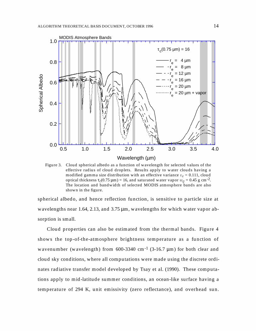
ALGORITHM THEORETICAL BASIS DOCUMENT, OCTOBER 1996 14
spherical albedo, and hence reflection function, is sensitive to particle size at
wavelengths near 1.64, 2.13, and 3.75 µm, wavelengths for which water vapor ab-
sorption is small.
Cloud properties can also be estimated from the thermal bands. Figure 4
shows the top-of-the-atmosphere brightness temperature as a function of
wavenumber (wavelength) from 600-3340 cm-1 (3-16.7 µm) for both clear and
cloud sky conditions, where all computations were made using the discrete ordi-
nates radiative transfer model developed by Tsay et al. (1990). These computa-
tions apply to mid-latitude summer conditions, an ocean-like surface having a
temperature of 294 K, unit emissivity (zero reflectance), and overhead sun.
0.0
0.2
0.4
0.6
0.8
1.0
0.5 1.0 1.5 2.0 2.5 3.0 3.5 4.0
Sph
eric
al A
lbed
o
Wavelength (µm)
cτ (0.75 µm) = 16
re = 4 µm
re = 8 µm
re = 12 µm
re = 16 µm
re = 20 µm
re = 20 µm + vapor
MODIS Atmosphere Bands
Figure 3. Cloud spherical albedo as a function of wavelength for selected values of theeffective radius of cloud droplets. Results apply to water clouds having amodified gamma size distribution with an effective variance ve = 0.111, cloudoptical thickness τc(0.75 µm) = 16, and saturated water vapor wg = 0.45 g cm-2.The location and bandwidth of selected MODIS atmosphere bands are alsoshown in the figure.

KING ET AL.: REMOTE SENSING OF CLOUD PROPERTIES FROM MODIS 15
These computations further include gaseous absorption (water vapor, carbon di-
oxide, ozone, and the infrared water vapor continuum) at a 20 cm-1 spectral
resolution (Tsay et al. 1989), with a low-level water cloud of optical thickness 5
(at 0.75 µm) placed at an altitude between 1 and 1.5 km.
In the 3.7 µm window, both solar reflected and thermal emitted radiation are
significant, though the use of the reflectance for cloud droplet size retrieval is
seen to be much more sensitive than the thermal component (note that, in either
case, the thermal and solar signals must be separated to provide the desired
Solar & Thermal (re = 8 µm)
Solar & Thermal (re = 16 µm)
Thermal (re = 8 µm)
240
260
280
300
320
340
1000 1500 2000 2500 3000
Clear Sky (overhead sun)
Thermal (re = 16 µm)
Brig
htne
ss T
empe
ratu
re (
K)
Wavenumber (cm-1)
Wavelength (µm)
16 12 10 8 6 5 4 3
O3
CO2CO2CO2 H2ON2OCH4
H2O
Figure 4. Brightness temperature as a function of wavelength for nadir observationsand for various values of the effective radius of cloud droplets, where thecloud optical thickness τc(0.75 µm) = 5 for all cases. Results apply to waterclouds having a modified gamma distribution embedded in a midlatitudesummer atmosphere with cloud top temperature Tt = 14°C, cloud base tem-perature Tb = 17°C, and an underlying surface temperature Ts = 21°C(assumed black). The location and bandwidth of all MODIS thermal bandsare also shown in the figure.

ALGORITHM THEORETICAL BASIS DOCUMENT, OCTOBER 1996 16
component). CO2 absorption is important around 4.3 µm and at wavelengths
greater than about 13 µm; the MODIS bands in these spectral regions can indicate
vertical changes of temperature.
Figure 5 shows the reflection function as a function of optical thickness and
effective radius for the MODIS Airborne Simulator bands used in cloud retrieval
validation studies. Calculations were performed using the optical constants of
liquid water compiled by Irvine and Pollack (1968), together with the assumption
that the underlying surface reflectance Ag = 0.0. As previously noted, the opti-
cal thickness of a cloud depends on wavelength as well as the cloud particle size
distribution n(r), as reflected in the effective radius [see King et al. (1990) for an
illustration of the spectral dependence of τc, g, s and τc′]. In order to compare the
0 5 10 15 20 25 30 35 40
d) 3.72 µm band
b) 1.62 µm bandR
efle
ctio
n F
unct
ion
Ref
lect
ion
Fun
ctio
n
0.0
0.2
0.4
0.6
0.8
1.0
0 5 10 15 20 25 30 35 40
Effective Optical Thickness
0.0
0.2
0.4
0.6
0.8
1.0a) 0.65 µm band
re = 1 µm
re = 4 µm
re = 6 µm
re =10 µm
re =20 µm
c) 2.14 µm band
Effective Optical Thickness
Figure 5. Reflection function as a function of effective optical thickness at a visiblewavelength for (a) 0.65 µm, (b) 1.62 µm, (c) 2.14 µm, and (d) 3.72 µm.
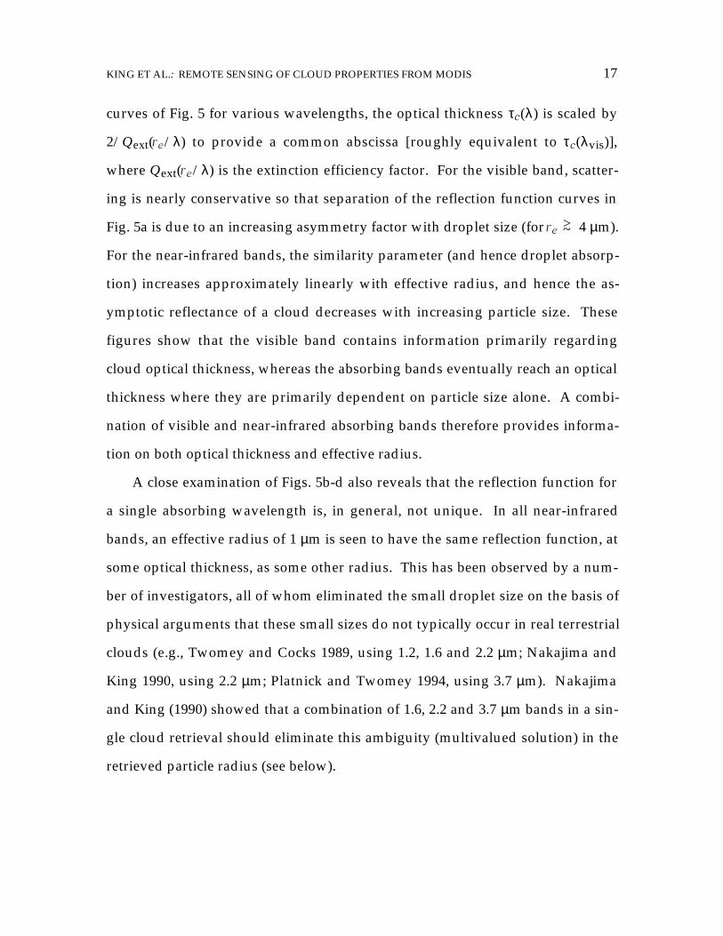
KING ET AL.: REMOTE SENSING OF CLOUD PROPERTIES FROM MODIS 17
curves of Fig. 5 for various wavelengths, the optical thickness τc(λ) is scaled by
2/Qext(re/λ) to provide a common abscissa [roughly equivalent to τc(λvis)],
where Qext(re/λ) is the extinction efficiency factor. For the visible band, scatter-
ing is nearly conservative so that separation of the reflection function curves in
Fig. 5a is due to an increasing asymmetry factor with droplet size (for re >~ 4 µm).
For the near-infrared bands, the similarity parameter (and hence droplet absorp-
tion) increases approximately linearly with effective radius, and hence the as-
ymptotic reflectance of a cloud decreases with increasing particle size. These
figures show that the visible band contains information primarily regarding
cloud optical thickness, whereas the absorbing bands eventually reach an optical
thickness where they are primarily dependent on particle size alone. A combi-
nation of visible and near-infrared absorbing bands therefore provides informa-
tion on both optical thickness and effective radius.
A close examination of Figs. 5b-d also reveals that the reflection function for
a single absorbing wavelength is, in general, not unique. In all near-infrared
bands, an effective radius of 1 µm is seen to have the same reflection function, at
some optical thickness, as some other radius. This has been observed by a num-
ber of investigators, all of whom eliminated the small droplet size on the basis of
physical arguments that these small sizes do not typically occur in real terrestrial
clouds (e.g., Twomey and Cocks 1989, using 1.2, 1.6 and 2.2 µm; Nakajima and
King 1990, using 2.2 µm; Platnick and Twomey 1994, using 3.7 µm). Nakajima
and King (1990) showed that a combination of 1.6, 2.2 and 3.7 µm bands in a sin-
gle cloud retrieval should eliminate this ambiguity (multivalued solution) in the
retrieved particle radius (see below).

ALGORITHM THEORETICAL BASIS DOCUMENT, OCTOBER 1996 18
b. Cloud thermodynamic phase
During the post-launch time period, we plan to perfect a robust and routine
algorithm for determining cloud thermodynamic phase (water vs ice). The
physical principle upon which this technique is based is the fact that the differ-
ences in reflected solar radiation between the 0.645 and 1.64 µm bands contain
information regarding cloud particle phase due to distinct differences in bulk ab-
sorption characteristics between water and ice at the longer wavelength. The
visible reflectance, suffering no appreciable absorption for either ice or liquid
water, is relatively unaffected by thermodynamic phase. However, if the cloud is
composed of ice, or if the surface is snow covered (similar in effect to large ice
particles), then the reflectance of the cloud at 1.64 µm will be smaller than for an
otherwise identical liquid water cloud. The 2.13 µm band is expected to show a
significant decrease in reflectance as well, but this is somewhat less dramatic
than the reduced reflectance at 1.64 µm. Demonstrations of the application of
this method to the problem of distinguishing the thermodynamic phase of clouds
can be found in Hansen and Pollack (1970), Curran and Wu (1982), and Pilewskie
and Twomey (1987). For added phase discrimination, it is expected that a re-
trieval of cloud effective radius using the 1.64 µm band alone will yield a sub-
stantially different result than one obtained using only the 2.13 µm band.
As an example of the sensitivity of the 1.64 and 2.13 µm bands of MODIS to
the thermodynamic phase of clouds, we have examined MAS data obtained over
the northern foothills of the Brooks Range, Alaska, on 8 June 1996. These data
were acquired as part of a NASA ER-2 airborne campaign to study arctic stratus
clouds over sea ice in the Beaufort Sea. The panel in the upper left portion of Fig.
6, acquired at 0.66 µm, shows high contrast between an optically thick convective
cumulonimbus cloud in the center of the image, a diffuse cirrus anvil in the

KING ET AL.: REMOTE SENSING OF CLOUD PROPERTIES FROM MODIS 19
lower part of the image, less reflective altocumulus clouds in the upper part of
the image, and dark tundra. From data obtained down the nadir track of the air-
craft (vertical line down the center of the image), we have produced scatter plots
of the ratio of the reflection function at 1.61, 1.88, and 2.13 µm to that at 0.66 µm
as a function of the brightness temperature at 11.02 µm. These observations
clearly shows that the cold portion of the scene contained ice particles (low re-
0.66 µm
230 240 250 260 27011 µm Brightness Temperature (K)
1.0
0.8
0.6
0.4
0.2
0.0
R(1
.61
µm)/
R(0
.66
µm)
0.8
0.6
0.4
0.2
0.0
R(2
.13
µm)/
R(0
.66
µm)
230 240 250 260 27011 µm Brightness Temperature (K)
0.0
0.3
0.2
0.1R(1
.88
µm)/
R(0
.66
µm) 0.4
0.5
Figure 6. The upper left-hand panel shows a MAS 0.66 µm image of a convective cu-mulonimbus cloud surrounded by lower-level water clouds on the northslope of the Brooks Range on 7 June 1996. Subsequent panels show scatterplots of the reflection function ratio R1.61/R0.66, R1.88/R0.66, and R2.13/R0.66
as a function of the corresponding brightness temperature at 11.02 µm fornadir observations of the MAS over a cloud scene containing both water andice clouds.
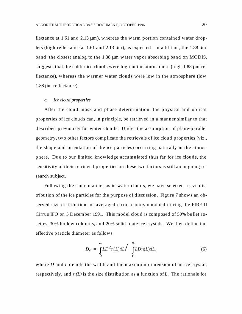
ALGORITHM THEORETICAL BASIS DOCUMENT, OCTOBER 1996 20
flectance at 1.61 and 2.13 µm), whereas the warm portion contained water drop-
lets (high reflectance at 1.61 and 2.13 µm), as expected. In addition, the 1.88 µm
band, the closest analog to the 1.38 µm water vapor absorbing band on MODIS,
suggests that the colder ice clouds were high in the atmosphere (high 1.88 µm re-
flectance), whereas the warmer water clouds were low in the atmosphere (low
1.88 µm reflectance).
c. Ice cloud properties
After the cloud mask and phase determination, the physical and optical
properties of ice clouds can, in principle, be retrieved in a manner similar to that
described previously for water clouds. Under the assumption of plane-parallel
geometry, two other factors complicate the retrievals of ice cloud properties (viz.,
the shape and orientation of the ice particles) occurring naturally in the atmos-
phere. Due to our limited knowledge accumulated thus far for ice clouds, the
sensitivity of their retrieved properties on these two factors is still an ongoing re-
search subject.
Following the same manner as in water clouds, we have selected a size dis-
tribution of the ice particles for the purpose of discussion. Figure 7 shows an ob-
served size distribution for averaged cirrus clouds obtained during the FIRE-II
Cirrus IFO on 5 December 1991. This model cloud is composed of 50% bullet ro-
settes, 30% hollow columns, and 20% solid plate ice crystals. We then define the
effective particle diameter as follows
De =
LD L L2 ( )n d
0
∞
∫ /
LD L Ln d( )0
∞
∫ , (6)
where D and L denote the width and the maximum dimension of an ice crystal,
respectively, and n(L) is the size distribution as a function of L. The rationale for

KING ET AL.: REMOTE SENSING OF CLOUD PROPERTIES FROM MODIS 21
defining De to represent ice-crystal size distribution is that the scattering of light
is related to the geometric cross section, which is proportional to LD. To calcu-
late properties of light scattering and absorption by ice crystals, we have adopted
a unified theory developed by Takano and Liou (1989, 1995), and Yang and Liou
(1995, 1996a,b) for all sizes and shapes. This unified theory is a unification of an
improved geometric ray-tracing/Monte Carlo method for size parameters larger
than about 15 and a finite-difference time domain method for size parameters
less than 15.
In Table 2, we demonstrate the bulk optical properties of this ice cloud
Par
ticle
Num
ber
Con
cent
ratio
n (li
ter-
1 µm
-1)
100
10-1
10-2
10-3
10-4
Maximum Dimension (µm)
0 100 200 300 400 500 600
50%
30%
20%
Figure 7. An averaged ice-crystal size distribution observed during the FIRE-II CirrusIFO (5 December 1991), as determined from the replicator sounding.

ALGORITHM THEORETICAL BASIS DOCUMENT, OCTOBER 1996 22
model, calculated for six selected MODIS bands. Their corresponding phase
functions are illustrated in Fig. 8. Thus, the reflected reflectance fields [e.g., Eq.
(5)] for ice clouds can be pre-computed for later use in retrieval algorithms simi-
lar to those of water clouds. It is worth noting that Ou et al. (1993) recently de-
veloped a retrieval technique that utilizes the thermal infrared emission of ice
clouds to determine their optical thickness and effective particle size. Removal of
the solar component in the 3.75 µm intensity is required for daytime applications,
which is made by correlating the 3.75 µm (solar) and 0.645 µm reflectances.
However, it is clear that the use of the reflectance for particle size retrieval is seen
from Fig. 4 to be much more sensitive than the thermal infrared component.
Careful intercomparison of cloud retrievals between these two methods is cur-
rently underway.
3.1.2. Mathematical description of algorithm
a. Asymptotic theory for thick layers
In the case of optically thick layers overlying a Lambertian surface, the ex-
pression for the reflection function of a conservative scattering atmosphere can
be written as (King 1987)
R(τc; µ, µ0, φ) = R∞(µ, µ0, φ) – 4(1–Ag)K(µ)K(µ0)
[ ]3(1–Ag)(1–g)(τc+2q0) + 4Ag , (7)
from which the scaled optical thickness τc′ can readily be derived:
Table 2. Optical properties of a representative ice crystal size distribution for six MODISbands.
Band λ(µm)
mr mi βe ω0 g
1 0.645 1.3082 1.325 × 10⁻⁸ 0.32827 0.99999 0.845805 1.240 1.2972 1.22 × 10⁻⁵ 0.33141 0.99574 0.852246 1.640 1.2881 2.67 × 10⁻⁴ 0.32462 0.93823 0.874247 2.130 1.2674 5.65 × 10⁻⁴ 0.32934 0.91056 0.8904420 3.750 1.3913 6.745 × 10⁻³ 0.32971 0.68713 0.9003031 11.030 1.1963 2.567 × 10⁻¹ 0.32812 0.54167 0.95739

KING ET AL.: REMOTE SENSING OF CLOUD PROPERTIES FROM MODIS 23
τc′ = (1–g)τc = 4K(µ)K(µ0)
3[ ]R∞(µ, µ0, φ) – R(τc; µ, µ0, φ) – 2q′ –
4Ag3(1–Ag) . (8)
In these expressions R(τc; µ, µ0, φ) is the measured reflection function at a
nonabsorbing wavelength, R∞(µ, µ0, φ) the reflection function of a semi-infinite
atmosphere, K(µ) the escape function, Ag the surface (ground) albedo, g the
asymmetry factor, and q0 the extrapolation length for conservative scattering.
The reduced extrapolation length q′ = (1−g)q0 lies in the range 0.709 to 0.715 for
all possible phase functions (van de Hulst 1980), and can thus be regarded as a
constant (q′ · 0.714).
From Eq. (8) we see that the scaled optical thickness of a cloud depends on q′,
50%
30%
20%
0.645 µm
1.240 µm
1.640 µm
2.130 µm
3.750 µm
11.03 µm
0 30 60 90 120 150 180
Scattering Angle
Sca
tterin
g P
hase
Fun
ctio
n103
102
101
100
10-1
10-2
Figure 8. Scattering phase functions for the ice cloud model shown in Fig. 7, calculatedfor six selected MODIS bands.

ALGORITHM THEORETICAL BASIS DOCUMENT, OCTOBER 1996 24
Ag, K(µ) and the difference between R∞(µ, µ0, φ) and the measured reflection func-
tion. At water-absorbing wavelengths outside the molecular absorption bands
(such as 1.64, 2.13 and 3.75 µm), the reflection function of optically thick atmos-
pheres overlying a Lambertian surface can be expressed as (King 1987)
R(τc; µ, µ0, φ) = R∞(µ, µ0, φ) – m (1–AgA*)l – Agmn
2 K(µ)K(µ0)e–2kτc
(1–AgA*)(1– l2e–2kτc) + Agmn
2le
–2kτc
, (9)
where k is the diffusion exponent (eigenvalue) describing the attenuation of ra-
diation in the diffusion domain, A* the spherical albedo of a semi-infinite atmos-
phere, and m, n and l constants. All five asymptotic constants that appear in this
expression [A*, m, n, l and k/(1−g)] are strongly dependent on the single scatter-
ing albedo ω0, with a somewhat weaker dependence on g. In fact, van de Hulst
(1974, 1980) and King (1981) showed that these constants can be well represented
by a function of a similarity parameter s, defined by Eq. (3), where s reduces to (1
− ω0)1/2 for isotropic scattering and spans the range 0 (ω0 = 1) to 1 (ω0 = 0).
Similarity relations for the asymptotic constants that arise in Eqs. (7-9) can be
found in King et al. (1990), and can directly be computed using eigenvectors and
eigenvalues arising in the discrete ordinates method (Nakajima and King 1992).
b. Retrieval example
To assess the sensitivity of the reflection function to cloud optical thickness
and effective radius, we performed radiative transfer calculations for a wide va-
riety of solar zenith angles and observational zenith and azimuth angles at se-
lected wavelengths in the visible and near-infrared. Figure 9a (9b) shows repre-
sentative calculations relating the reflection functions at 0.664 and 1.621 µm
(2.142 µm). These wavelengths were chosen because they are outside the water
vapor and oxygen absorption bands and yet have substantially different water

KING ET AL.: REMOTE SENSING OF CLOUD PROPERTIES FROM MODIS 25
droplet (or ice particle) absorption characteristics (cf. Fig. 2). These wavelengths
correspond to three bands of the MAS, but may readily be adapted to the compa-
rable 0.645, 1.64, 2.13 and 3.75 µm bands of MODIS.
Figure 9 clearly illustrates the underlying principles behind the simultaneous
determination of τc and re from reflected solar radiation measurements. The
0.0
0.2
0.4
0.6
0.8
1.0
re = 2 µm
0.0 0.2 0.4 0.6 0.8 1.0
32 µm
16 µm
8 µm
4 µm
3224161284
2
486
80
b
0.0
0.2
0.4
0.6
0.8
1.0
32 µm
16 µm
8 µm
4 µm
re = 2 µm
32241612
8
42
τc
48
6
80
θ0 = 26°, θ = 40°, φ = 42°
a
Ref
lect
ion
Fun
ctio
n (1
.621
µm
)
Reflection Function (0.664 µm)
τc
Ref
lect
ion
Fun
ctio
n (2
.142
µm
)
Figure 9. Theoretical relationship between the reflection function at 0.664 and (a) 1.621µm and (b) 2.142 µm for various values of τc (at 0.664 µm) and re when θ0 =26°, θ = 40° and φ = 42°. Data from measurements above marine stratocumu-lus clouds during ASTEX are superimposed on the figure (22 June 1992).

ALGORITHM THEORETICAL BASIS DOCUMENT, OCTOBER 1996 26
minimum value of the reflection function at each wavelength corresponds to the
reflection function of the underlying surface at that wavelength in the absence of
an atmosphere. For the computations presented in Fig. 9, the underlying surface
was assumed to be Lambertian with Ag = 0.06, 0.05, and 0.045 for wavelengths of
0.664, 1.621, and 2.142 µm, respectively, roughly corresponding to an ocean sur-
face. The dashed curves in Fig. 9 represent the reflection functions at 0.664, 1.621
and 2.142 µm that result for specified values of the cloud optical thickness at
0.664 µm. The solid curves, on the other hand, represent the reflection functions
that result for specified values of the effective particle radius. These results
show, for example, that the cloud optical thickness is largely determined by the
reflection function at a nonabsorbing wavelength (0.664 µm in this case), with
little dependence on particle radius. The reflection function at 2.142 µm (or 1.621
µm), in contrast, is largely sensitive to re, with the largest values of the reflection
function occurring for small particle sizes. In fact, as the optical thickness in-
creases (τc >~ 12), the sensitivity of the nonabsorbing and absorbing bands to
τc(0.664 µm) and re is very nearly orthogonal. This implies that under these opti-
cally thick conditions we can determine the optical thickness and effective radius
nearly independently, and thus measurement errors in one band have little im-
pact on the cloud optical property determined primarily by the other band. The
previously described multiple solutions are clearly seen as re and τc decrease.
The data points superimposed on the theoretical curves of Fig. 9 represent
over 400 measurements obtained with the MAS, a 50-band scanning spectrome-
ter that was mounted in the right wing superpod of the NASA ER-2 aircraft
during ASTEX. These observations were obtained as the aircraft flew over ma-
rine stratocumulus clouds in the vicinity of the Azores approximately 1000 km
southwest of Lisbon on 22 June 1992.

KING ET AL.: REMOTE SENSING OF CLOUD PROPERTIES FROM MODIS 27
c. Atmospheric corrections: Rayleigh scattering
As discussed in the previous section, the sensor-measured intensity at visible
wavelengths (0.66 µm) is primarily a function of cloud optical thickness, whereas
near-infrared intensities (1.6, 2.1, and 3.7 µm) are sensitive both to optical thick-
ness and, especially, cloud particle size. As a consequence, Rayleigh scattering in
the atmosphere above the cloud primarily affects the cloud optical thickness re-
trieval since the Rayleigh optical thickness in the near-infrared is negligible. Be-
cause the Rayleigh optical thickness in the visible wavelength region is small
(about 0.044 at 0.66 µm), it is frequently overlooked in retrieving cloud optical
thickness.
We simplified the air-cloud system as a two-layer atmosphere with mole-
cules above the cloud, and carried out simulations with an adding-doubling code
to investigate the Rayleigh scattering effects on cloud optical thickness retrievals.
Figures 10a and 10b provide typical errors ∆τc (%) in retrieved cloud optical
thickness τc without making any Rayleigh corrections. These errors apply to a
cloud with an effective particle radius re = 8 µm. Figure 10a applies to errors ∆τc
at different solar and viewing zenith angles when τc = 2, whereas Figure 10b
pertains to ∆τc for different solar angles and various cloud optical thicknesses
when the viewing zenith angle θ = 45.2°. Figure 10a shows that, for thin clouds,
∆τc ranges from 15 to 60% for solar and viewing angles ranging from 0-80°. Er-
rors increase with increasing solar and/or viewing angles because of enhanced
Rayleigh scattering contributions at large angles. On the other hand, Figure 10b
shows that, for thick clouds, ∆τc can still be as high as 10-60% for solar zenith an-
gles θ0 ≥ 60°. Therefore, it is important to correct for Rayleigh scattering contri-
butions to the reflected signal from a cloud layer both for (i) the case of thin
clouds, and (ii) for large solar zenith angles and all clouds.

ALGORITHM THEORETICAL BASIS DOCUMENT, OCTOBER 1996 28
We developed an iterative method for effectively removing Rayleigh scat-
tering contributions from the measured intensity signal in cloud optical thickness
retrievals (Wang and King 1997). In brief, by assuming that no multiple scatter-
ing occurs in the Rayleigh layer, we decomposed the sensor-measured upward
100
10
4
10
10
-3
1
6020
40
10
1 0 -1 -2
Viewing zenith angle
Sol
ar z
enith
ang
le
10 20 30 40 50 60
Cloud optical thickness
Sol
ar z
enith
ang
le
12
60
100
16
17
35
6023 35
60
3523 23
17 17
15
1516
15
10 20 30 40 50 60 70 80
80
70
60
50
40
30
20
10
0
τc = 2
θ = 45.2°
a
b80
70
60
50
40
30
20
10
0
Figure 10. Error ∆τc (%) in retrieved cloud optical thickness without Rayleigh correctionsfor (a) τc = 2 and (b) θ = 45.2°. The azimuth angle φ = 90° in both cases.
KING ET AL.: REMOTE SENSING OF CLOUD PROPERTIES FROM MODIS 29
reflection function of the two-layer air-cloud atmosphere at the top of the atmos-
phere arising from (i) direct Rayleigh single scattering without reflection from
the cloud, (ii) contributions of single interactions between air molecules and
clouds, and (iii) reflection of the direct solar beam from the cloud. By removing
contributions (i) and (ii) from the sensor-measured reflection function, we were
able to derive iteratively the cloud top reflection function in the absence of
Rayleigh scattering for use in cloud optical thickness retrievals. The Rayleigh
correction algorithm has been extensively tested for realistic cloud optical and
microphysical properties with different solar zenith angles and viewing
geometries. From simulated results we concluded that, with the proposed
Rayleigh correction algorithm, the error in retrieved cloud optical thickness was
reduced by a factor of 2 to over 10 for both thin clouds as well as thick clouds
with large solar zenith angles. The iteration scheme is efficient and has been in-
corporated into our cloud retrieval algorithm.
d. Atmospheric corrections: Water vapor
The correlated k-distribution of Kratz (1995) can be used to calculate the
gaseous atmospheric transmission and/or emission for all MODIS bands. The
primary input for this code is an atmospheric temperature and water vapor pro-
file for the above-cloud portion of the atmosphere. It is expected that tempera-
ture and humidity can be provided by NCEP, DAO, or MOD07 (for the nearest
clear sky pixel), as discussed in Section 3.3.1.b. Alternatively, it may turn out
that many of the MODIS bands are not particularly sensitive to the distribution
of water vapor, but only to the column amount. For such bands, above-cloud
precipitable water estimates from MOD05 may be sufficient. Estimates of ozone
amount, from either MOD07 or ancillary sources, will be needed for the 0.645 µm

ALGORITHM THEORETICAL BASIS DOCUMENT, OCTOBER 1996 30
band if standard values prove insufficient.
The effects of the atmosphere need to be removed so that the cloud-top re-
flectance and/or emission can be determined. It is these cloud-top quantities
that are stored in the libraries of Fig. 11 (see below). Ignoring Rayleigh or aerosol
scattering, gaseous absorption in the above-cloud atmosphere can be accounted
for with the following equation (Platnick and Valero 1995):
I(µ, µ0, φ) = I clo topsolar
ud− (τc, re, Ag; µ, µ0, φ) tatm(µ) tatm(µ0)
+ I atmsolar (µ, µ0, φ) + I clou top
emissiond− (τc, re, Ag; µ) tatm(µ)
` + I atmemission(µ), (10)
where I is the measured intensity at the top-of-atmosphere, Icloud-top is the cloud-
top intensity, including surface effects, in the absence of an atmosphere, and tatm
is the above-cloud transmittance in either the µ or µ0 directions. In general, both
the cloud and atmosphere contribute emitted (Iemission) and solar scattered
(Isolar) radiant energy. The first term accounts for the effect of the atmosphere on
the net cloud-surface reflectance and the third term the effect of cloud and sur-
face emission. For the 3.75 µm band both scattered solar and emitted thermal
terms are needed; for shorter wavelength bands, only solar terms are needed; in
the thermal infrared, only emission terms are needed.
Though not strictly correct, it is assumed that in practice this gaseous ab-
sorption layer can be treated as separate from the Rayleigh scattering layer de-
scribed above (or any aerosol layer), such that the specific corrections can be ap-
plied independently.
e. Technical outline of multi-band algorithm
A generalized schematic description of the cloud retrieval algorithm is given
in Figs. 11-13. Figure 11 shows the steps involved in calculating the reflection
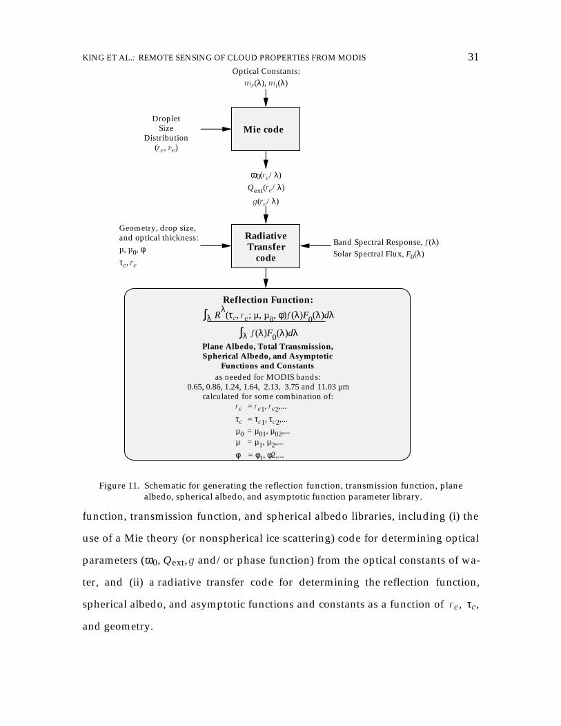
KING ET AL.: REMOTE SENSING OF CLOUD PROPERTIES FROM MODIS 31
function, transmission function, and spherical albedo libraries, including (i) the
use of a Mie theory (or nonspherical ice scattering) code for determining optical
parameters (ω0, Qext, g and/or phase function) from the optical constants of wa-
ter, and (ii) a radiative transfer code for determining the reflection function,
spherical albedo, and asymptotic functions and constants as a function of re, τc,
and geometry.
Optical Constants:mr(λ), mi(λ)
DropletSize
Distribution(re, ve)
Band Spectral Response, f(λ)Solar Spectral Flux, F0(λ)
Mie code
ω0(re/λ)Qext(re/λ)
g(re/λ)
Geometry, drop size, and optical thickness:µ, µ0, φτc, re
Radiative Transfer
code
Reflection Function:
∫λ Rλ(τc, re; µ, µ0, φ)f(λ)F0(λ)dλ
∫λ f(λ)F0(λ)dλ
as needed for MODIS bands: 0.65, 0.86, 1.24, 1.64, 2.13, 3.75 and 11.03 µm
calculated for some combination of:re = re1, re2,...
τc = τc1, τc2,...µ0 = µ01, µ02,...µ = µ1, µ2,...
φ = φ1, φ2,...
Plane Albedo, Total Transmission, Spherical Albedo, and Asymptotic
Functions and Constants
Figure 11. Schematic for generating the reflection function, transmission function, planealbedo, spherical albedo, and asymptotic function parameter library.
ALGORITHM THEORETICAL BASIS DOCUMENT, OCTOBER 1996 32
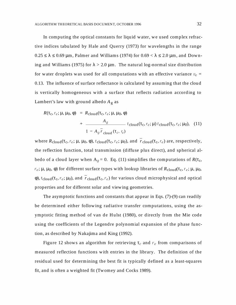
In computing the optical constants for liquid water, we used complex refrac-
tive indices tabulated by Hale and Querry (1973) for wavelengths in the range
0.25 ≤ λ ≤ 0.69 µm, Palmer and Williams (1974) for 0.69 < λ ≤ 2.0 µm, and Down-
ing and Williams (1975) for λ > 2.0 µm. The natural log-normal size distribution
for water droplets was used for all computations with an effective variance ve =
0.13. The influence of surface reflectance is calculated by assuming that the cloud
is vertically homogeneous with a surface that reflects radiation according to
Lambert’s law with ground albedo Ag as
R(τc, re; µ, µ0, φ) = Rcloud(τc, re; µ, µ0, φ)
+
A
A r_
,
g
g c er1 ( )cloud− τ
tcloud(τc, re; µ) tcloud(τc, re; µ0), (11)
where Rcloud(τc, re; µ, µ0, φ), tcloud(τc, re; µ0), and r_
cloud(τc, re) are, respectively,
the reflection function, total transmission (diffuse plus direct), and spherical al-
bedo of a cloud layer when Ag = 0. Eq. (11) simplifies the computations of R(τc,
re; µ, µ0, φ) for different surface types with lookup libraries of Rcloud(τc, re; µ, µ0,
φ), tcloud(τc, re; µ0), and r_
cloud(τc, re) for various cloud microphysical and optical
properties and for different solar and viewing geometries.
The asymptotic functions and constants that appear in Eqs. (7)-(9) can readily
be determined either following radiative transfer computations, using the as-
ymptotic fitting method of van de Hulst (1980), or directly from the Mie code
using the coefficients of the Legendre polynomial expansion of the phase func-
tion, as described by Nakajima and King (1992).
Figure 12 shows an algorithm for retrieving τc and re from comparisons of
measured reflection functions with entries in the library. The definition of the
residual used for determining the best fit is typically defined as a least-squares
fit, and is often a weighted fit (Twomey and Cocks 1989).

KING ET AL.: REMOTE SENSING OF CLOUD PROPERTIES FROM MODIS 33
The use of the 3.75 µm band complicates the algorithm because radiation
emitted by the cloud is comparable to, and often dominates, the solar reflectance.
Cloud emission at 3.75 µm is weakly dependent on re, unlike solar reflectance (cf.
Fig. 4), so the relative strength of the two depends on particle size. Surface emis-
sion can also be significant for thin clouds (τc <~ 5). For example, with cloud and
surface temperatures of 290 K, emission and reflectance are approximately equal
for re = 10 µm (Platnick and Twomey 1994). An assumption that is often made is
Visible & NIR Measurements
(intensity or bidirectional reflectance):
Exo-atmospheric solar spectral flux for each band with radiance measurement
Assumed/inferred above-cloud atmosphere: e.g., atmospheric transmission and Rayleigh scattering corrections
Visible & NIR Atmospheric
Correction
Determine combination τcm, ren that minimizes error
Determine Geometry and Surface Albedo
for each pixel:µ, µ0, φ, Ag(λ)
Calculated libraries forτc =τc1, τc2,…,τcMre = re1, re2,…,reN
Residual Definition:
[lnRmeas(µ, µ0, φ) – lnRcalc(τcm, ren; µ, µ0, φ)]visvis 2
+ [lnRmeas(µ, µ0, φ) – lnRcalc(τcm, ren; µ, µ0, φ)]NIRNIR 2
Rmeas(µ, µ0, φ)
Rmeas(µ, µ0, φ)
Rmeas(µ, µ0, φ)
Rmeas(µ, µ0, φ)
Rmeas(µ, µ0, φ)
0.65
0.86
1.24
1.64
2.13
Rcalc(τcm, ren; µ, µ0, φ)
Rcalc(τcm, ren; µ, µ0, φ)
Rcalc(τcm, ren; µ, µ0, φ)
Rcalc(τcm, ren; µ, µ0, φ)
Rcalc(τcm, ren; µ, µ0, φ)
Rcalc(τcm, ren; µ, µ0, φ)
0.65
0.86
1.24
1.64
2.13
3.75
Figure 12. A general cloud retrieval algorithm for determining best fit for τc and re in the0.65, 1.64 and 2.13 µm bands.

ALGORITHM THEORETICAL BASIS DOCUMENT, OCTOBER 1996 34
that clouds are isothermal. Retrievals using this band include those made by
Arking and Childs (1985), Grainger (1990), Platnick (1991), Kaufman and Naka-
jima (1993), Han et al. (1994, 1995), Platnick and Valero (1995), and Nakajima and
Nakajima (1995), all of whom used the visible and 3.7 µm bands of AVHRR.
To correct for thermal emission in the 3.75 µm band, we decomposed the to-
tal upward reflection function at the top of the atmosphere into solar, thermal,
and surface contributions. Ignoring atmospheric effects above the cloud, which
can readily be corrected as described above for both water vapor and Rayleigh
scattering effects, we can write the total above-cloud measured reflection func-
tion as (Platnick and Valero 1995; Nakajima and Nakajima 1995)
Rmeas(τc, re; µ, µ0, φ) = Rcloud(τc, re; µ, µ0, φ)
+
A
A r_
,
g
g c er1 ( )cloud− τ
tcloud(τc, re; µ) tcloud(τc, re; µ0)
+ ε cloud* (τc, re; µ) B(Tc)
πµ0 0F
+ ε surface* (τc, re; µ) B(Tg)
πµ0 0F
. (12)
In this equation, the first two terms account for solar reflectance and are
identical to Eq. (11), ε surface* (τc, re; µ) is the effective surface emissivity that in-
cludes the effect of the cloud on radiation emitted by the surface, and ε cloud* (τc,
re; µ) is the effective cloud emissivity that can be formulated to include cloud
emission that is reflected by the surface. These emissivities are given by
ε cloud* (τc, re; µ) = [1 – tcloud(τc, re; µ) – rcloud(τc, re; µ)]
+ surface interaction terms, (13)
ε surface* (τc, re; µ) =
1 – A
A r_
,
g
g c er1 ( )cloud− τ
tcloud(τc, re; µ), (14)
where rcloud(τc, re; µ) is the plane albedo of the cloud, and B(Tc) and B(Tg) are,
respectively, the Planck function at cloud top temperature Tc and surface tem-

KING ET AL.: REMOTE SENSING OF CLOUD PROPERTIES FROM MODIS 35
perature Tg.
The terms on the right-hand side of Eq. (12) pertain, in turn, to (i) solar re-
flection by the cloud in the absence of surface reflection, (ii) contributions from
multiple reflection of solar radiation by the Earth’s surface, (iii) thermal emission
from the cloud, and (iv) thermal emission from the surface. For thin clouds (τc <~
5), the second and fourth terms dominate, with surface emission contributing
over 50% of the total measured intensity. For thick clouds (τc > 10), on the other
hand, the first and third terms are the most important. The surface interaction
terms in the effective cloud emissivity account for downward emitted cloud ra-
diation reflected by the surface and back through the cloud. This is generally in-
significant except for perhaps the optically thinnest clouds. The cloud top tem-
perature Tc can be obtained either as an output of Menzel and Strabala’s (1997)
MODIS cloud top property algorithm or from output of the Data Assimilation
Office algorithm (DAO 1996), as discussed in Section 3.3.1.b. Surface tempera-
ture Tg is also required under cloudy conditions, and we intend to obtain this pa-
rameter from various sources, depending on whether the pixel is over land or
water (cf. Section 3.3.1.b). This is only a serious problem for optically thin (i.e.,
cirrus) clouds.
The thermal emission from the atmosphere above the cloud [the fourth term
in Eq. (10)] is usually of second order importance, contributing only a few per-
cent to the total intensity. This emission can be expressed as
Ratm(µ) = – ( ( )) d ( ; )atm
πµ
µ∫0 0 0
0
FB T p t p
p
, (15)
≈
πµ0 0F
[1 – tatm(µ)] B(Ta), (16)
where p0 is the cloud top pressure and Ta is an appropriate atmospheric tem-

ALGORITHM THEORETICAL BASIS DOCUMENT, OCTOBER 1996 36
perature. For a given temperature and moisture profiles, either obtained from
Menzel and Gumley’s (1997) MODIS atmospheric profiles product (cf. Fig. 1), or
from an NCEP or DAO gridded data set, we can calculate the Ratm(µ) term using
Eq. (15). An alternative approach is to use Eq. (16) with a given total water-vapor
loading above the cloud and some averaged atmospheric temperature. This
probably will be accurate enough because of relatively small thermal contribu-
tions from the atmosphere. By removing the thermal contributions (the third
and fourth terms) from the sensor-measured intensity, the 3.75 µm algorithm op-
erates in a manner quite similar to that for the 1.64 and 2.13 µm bands.
We plan on utilizing Nakajima and King’s (1990) algorithm for retrieving the
cloud optical thickness and effective radius using the 1.64 and 2.13 µm bands, to-
gether with a similar algorithm based on Platnick (1991) and Nakajima and
Nakajima (1995) for removing the thermal contributions from the 3.75 µm band,
as outlined above and in Figure 13.
f. Retrieval of cloud optical thickness and effective radius
In the description of the algorithm that follows, all subsequent references to
τc will be scaled, or normalized, to an optical thickness at 0.65 µm (or
2/Qext(re/λ), used previously in Fig. 5). In order to implement the Nakajima and
King algorithm, it is first necessary to compute the reflection function, plane al-
bedo, total transmission, and spherical albedo for the standard problem of plane-
parallel homogeneous cloud layers (Ag) with various τc′ and re = 2(n+1)/4 for n =
5, ..., 19, assuming a model cloud particle size distribution such as a log-normal
size distribution. We have generated the reflection function libraries for τc′ = 0.4,
0.8, 1.2 and ∞ (τc = 3, 5, 8 and ∞), flux libraries for τc′ = 0.4, 0.8, and 1.2, and a li-
brary for asymptotic functions and constants. These values of τc′ are selected
such that interpolation errors are everywhere ≤ 3% for τc′ ≥ 0.6 (τc · 4). This was

KING ET AL.: REMOTE SENSING OF CLOUD PROPERTIES FROM MODIS 37
accomplished using a combination of asymptotic theory for τc′ ≥ 1.8 (τc · 12) and
spline under tension interpolation for τc′ < 1.8.
The interpolation scheme reduces the number of library optical thickness
entries substantially, but replaces those entries with a combination of spline in-
Determine Geometry and Surface Albedo
for each pixel:µ, µ0, φ, Ag(λ)
Thermal IR(intensity or temperature)
εs (τcm, ren; µ)calc
εc (τcm, ren; µ)calc
εs (τcm, ren; µ)calc
3.75
3.75
IR
εc (τcm, ren; µ)calcIR
3.75 µm Atmospheric
Correction
}
3.75Rcalc(τcm, ren; µ, µ0, φ)
Calculated libraries forτc =τc1, τc2,…,τcMre = re1, re2,…,reN Ts
}Tc(τcm, ren; µ) from IR
3.75 µm emission at cloud top
for (τcm, ren; µ)
Thermal IR Atmospheric
Correction
3.75 µm Intensity Measurement
to residual definition to residual definition
Rmeas(τcm, ren; µ, µ0, φ)3.75
Figure 13. A general cloud retrieval algorithm for determining best fit for τc and re in the3.75 µm band.

ALGORITHM THEORETICAL BASIS DOCUMENT, OCTOBER 1996 38
terpolation and asymptotic formulae, depending on optical thickness. Calcula-
tions of the reflection function can be performed using the discrete ordinates
method formulated by Nakajima and Tanaka (1986) or Stamnes et al. (1988). The
asymptotic functions and constants that appear in Eqs. (7)–(9) can be obtained
from solutions of an eigenvalue equation that arises in the discrete ordinates
method (Nakajima and King 1992).
If one assumes that each reflection function measurement is made with equal
relative precision, maximizing the probability that R measi (µ, µ0, φ) observations
have the functional form R calci (τc, re; µ, µ0, φ) is equivalent to minimizing the
statistic χ2, defined as (Nakajima and King 1990)
χ2 =
i
∑ [ln R measi (µ, µ0, φ) – ln R calc
i (τc, re; µ, µ0, φ)]2, (17)
where the summation extends over all wavelengths λ i for which measurements
have been made and calculations performed.
Minimizing χ2 as defined by Eq. (17) is equivalent to making an unweighted
least-squares fit to the data (Bevington 1969). The minimum value of χ2 can be
determined by setting the partial derivatives of χ2 with respect to each of the co-
efficients [τc(0.65 or 0.75 µm), re] equal to zero. Due to the complicated depend-
ence of the reflection function on τc and re, however, this solution is nonlinear in
the unknowns τc and re such that no analytic solution for the coefficients exists.
Even for optically thick layers, where asymptotic theory applies, R ∞i (re; µ, µ0, φ)
is a complicated function of the phase function, and hence re, as King (1987) has
shown by deriving the cloud optical thickness assuming the clouds had two dif-
ferent phase functions but the same asymmetry factor.
In order to solve this nonlinear least-squares problem, we have adopted a
procedure whereby the scaled optical thickness τc′, and hence τc and g, is deter-
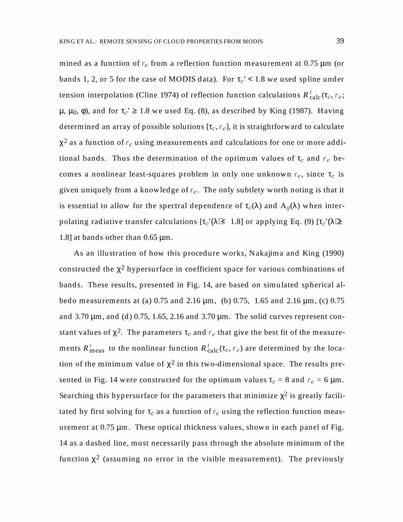
KING ET AL.: REMOTE SENSING OF CLOUD PROPERTIES FROM MODIS 39
mined as a function of re from a reflection function measurement at 0.75 µm (or
bands 1, 2, or 5 for the case of MODIS data). For τc′ < 1.8 we used spline under
tension interpolation (Cline 1974) of reflection function calculations R calci (τc, re;
µ, µ0, φ), and for τc′ ≥ 1.8 we used Eq. (8), as described by King (1987). Having
determined an array of possible solutions [τc, re], it is straightforward to calculate
χ2 as a function of re using measurements and calculations for one or more addi-
tional bands. Thus the determination of the optimum values of τc and re be-
comes a nonlinear least-squares problem in only one unknown re, since τc is
given uniquely from a knowledge of re. The only subtlety worth noting is that it
is essential to allow for the spectral dependence of τc(λ) and Ag(λ) when inter-
polating radiative transfer calculations [τc′(λ) < 1.8] or applying Eq. (9) [τc′(λ) ≥
1.8] at bands other than 0.65 µm.
As an illustration of how this procedure works, Nakajima and King (1990)
constructed the χ2 hypersurface in coefficient space for various combinations of
bands. These results, presented in Fig. 14, are based on simulated spherical al-
bedo measurements at (a) 0.75 and 2.16 µm, (b) 0.75, 1.65 and 2.16 µm, (c) 0.75
and 3.70 µm, and (d) 0.75, 1.65, 2.16 and 3.70 µm. The solid curves represent con-
stant values of χ2. The parameters τc and re that give the best fit of the measure-
ments R measi to the nonlinear function R calc
i (τc, re) are determined by the loca-
tion of the minimum value of χ2 in this two-dimensional space. The results pre-
sented in Fig. 14 were constructed for the optimum values τc = 8 and re = 6 µm.
Searching this hypersurface for the parameters that minimize χ2 is greatly facili-
tated by first solving for τc as a function of re using the reflection function meas-
urement at 0.75 µm. These optical thickness values, shown in each panel of Fig.
14 as a dashed line, must necessarily pass through the absolute minimum of the
function χ2 (assuming no error in the visible measurement). The previously

ALGORITHM THEORETICAL BASIS DOCUMENT, OCTOBER 1996 40
mentioned multiple solutions are readily seen for small τc and re, though the
ambiguity is eliminated in Fig. 14d when using all available near-infrared bands.
We are currently retrieving τc and re separately using pairs of bands, an ap-
propriate optical thickness-sensitive band, together with an appropriate near-
infrared band (e.g., vis and 1.64 µm, vis and 2.13 µm, and vis and 3.75 µm), since
each near-infrared band is sensitive to the effective radius at a different depth
within the cloud (Platnick 1997). The lowest (optical thickness-sensitive) band
Figure 14. χ2 hypersurface for theoretically generated spherical albedo measurements at(a) 0.75 and 2.16 µm, (b) 0.75, 1.65 and 2.16 µm, (c) 0.75 and 3.70 µm, and (d)0.75, 1.65, 2.16 and 3.70 µm. The solid curves represent constant values of χ2,while the dashed curve in each panel represents the array of possible solu-tions for R meas
.0 75 = 0.495. These results were constructed for a model cloudlayer having τc(0.75 µm) = 8 and re = 6 µm, located by the minimum value ofχ2 in this two-dimensional space [from Nakajima and King (1990)].
KING ET AL.: REMOTE SENSING OF CLOUD PROPERTIES FROM MODIS 41
will be either 0.65 µm over land, 0.86 µm over water, or 1.24 µm over snow and
sea ice surfaces. For water clouds, the effective radius typically increases from
cloud base to cloud top, with the 3.75 µm retrieval being the most sensitive to
drops high in the cloud and 1.64 µm much lower in the cloud. For ice clouds, the
vertical profile of effective radius is just the opposite, with the smallest crystals
highest in the cloud. Although the χ2 multi-band retrieval algorithm described
above has the merit of eliminating multiple solutions, the effective radius thus
obtained in realistic, vertically inhomogeneous clouds, is some compromise in
effective radius. We are thus doing multiple retrievals using the similarity (or
differences) in the retrieved results as a quality control indicator in the output
data product (cf. Table 5). If the differences between retrievals are excessively
large (i.e., ∆re >~ 2 µm), then we will switch to an ice retrieval algorithm that is
identical to the one outlined above, but with an ice crystal phase function rather
than water droplet phase function in the look-up tables.
3.2. Variance and uncertainty estimates
The overall uncertainties in determining the cloud optical thickness and ef-
fective radius can loosely be categorized as originating in either the model used
for developing the cloud reflection function and emittance libraries, or in the
physical uncertainties brought about through changing instrument error and at-
mospheric effects. Though it is difficult to draw the line between the two, it is
convenient to consider the model uncertainties to have their source in the library
generating algorithm shown schematically in Fig. 11 and the algorithm used for
approximating emitted thermal radiation at 3.75 µm. The physical uncertainties
can be largely ascribed to the atmospheric correction boxes and the measured
data shown in Fig. 12.
ALGORITHM THEORETICAL BASIS DOCUMENT, OCTOBER 1996 42
3.2.1. Model uncertainties
Several sources of model error are potentially significant. First of all, the
treatment of the wavelength integration over the bandpass filters is important
because it impacts calculations of the spectral reflection functions and emissivi-
ties. Ideally, the spectral integration should be based on the variability of the
optical constants across the bandpass filter. For example, the absorption of liquid
water, as measured by the imaginary part of the complex refractive index of wa-
ter, varies significantly throughout the near-infrared wavelength region, whereas
the real part of the refractive index is approximately constant over this region.
Mie calculations are dependent on the size parameter (2πr/λ), thereby adding
another wavelength dependence. For computational reasons, it is desirable to
determine the minimum number of wavelengths needed in any retrieval.
In order to assess the impact of finite bandpass characteristics of the MODIS
bands on our cloud retrieval algorithm, we performed calculations of the reflec-
tion function using 11 equally-spaced wavelengths for each band. These results
were then compared with reflection function computations based on a single
wavelength at the bandpass center. Ultimately, however, it is the effect of the
wavelength integration on the retrieval of τc and re that is important, not the ab-
solute changes in the reflection functions themselves. Since the near-infrared re-
flection functions are more sensitive to the finite bandpass characteristics of
MODIS, we restrict our analysis to the retrieval of re.
Figure 15 shows the error in the retrieval of re when using a single wave-
length calculation for the 2.14 µm band of MAS, where the 11 wavelength inte-
gration over the bandpass characteristics of the band is taken as the “true solu-
tion.” The optical thickness is such that the asymptotic reflection function has
been reached for most radii. This choice of optical thickness gives a conservative

KING ET AL.: REMOTE SENSING OF CLOUD PROPERTIES FROM MODIS 43
estimate of retrieval error since the sensitivity of re to reflection function is the
smallest. Figure 15 shows that using the wavelength of the peak of the spectral
bandpass is sufficient for obtaining effective radii errors within 0.5 µm.
Another approach one might take is to spectrally integrate the optical pa-
rameters ωλ0 , Qλ
ext , and gλ over wavelength and use these results for a single
wavelength retrieval. This comparison is shown in Fig. 16 for the same MAS
band as shown in Fig. 15. For τc = 50, the error is less that 0.1 µm for the ex-
pected range of effective radii to be encountered in terrestrial clouds. For an op-
tically thin cloud (τc = 1) the error increases to 0.3 µm at re = 4 µm. However, for
Effe
ctiv
e ra
dius
(µm
) de
term
ined
by
sin
gle
wav
elen
gth
calc
ulat
ion
MAS band 20
Wavelength at 100%channel response
Wavelength (µm)
-1.00
1.00
-0.50
0.00
0.50
2.003.00 -1.50-2.00
2.12 2.13 2.14 2.15 2.16 2.17 2.18
0
5
10
15
20
25
Figure 15. Error in the retrieval of re (µm) between (i) using spectrally averaged reflec-tion functions, sensor and solar weighted with 11 wavelengths, and (ii) a sin-gle wavelength calculation. These results apply to the MAS 2.14 µm bandwith µ0 = 0.75, µ = 0.95, τc = 50, and the optical constants of Irvine and Pollack(1968).

ALGORITHM THEORETICAL BASIS DOCUMENT, OCTOBER 1996 44
such an optically thin cloud, uncertainties in surface reflectance and atmospheric
corrections are likely to dominate this error. Similar results were obtained when
analyzing MAS 1.62 and 3.73 µm bands. At this time, it appears that an integra-
tion over ωλ0 , Qλ
ext , and gλ will provide an adequate reflectance library. Table 3
summarizes the maximum retrieval errors in re for all near-infrared bands (based
on calculations at µ0 = 0.95, 0.75, 0.5, µ = 0.95 and τc = 1, 5, 50). Effects of spectral
integration on emission in the 3.7 µm bands are not included in Table 3.
The effect of a shift in the central wavelength of the near-infrared bands can
also be assessed. For each band, the reflection function changes arising from a
Effective Radius (µm)
-0.4
-0.3
-0.2
-0.1
0.0
0.1
0.2
0 10 20 30 40 50
Err
or in
Ret
rieve
d R
adiu
s (µ
m)
MAS Band 20 (2.14 µm)
µ0 = 0.75, τc = 1µ0 = 0.75, τc = 50
µ0 = 0.45, τc = 50µ0 = 0.45, τc = 1
µ0 = 0.95, τc = 1µ0 = 0.95, τc = 50
Figure 16. Error in the retrieval of re (µm) between (i) using spectrally averaged reflec-tion functions, sensor and solar weighted with 11 wavelengths, and (ii) usingreflection function calculations based on spectral averages of cloud opticalproperties (ωλ
0 , Qλext , and gλ). These results were obtained using the MAS
2.14 µm band with µ = 0.95 and the optical constants of Irvine and Pollack(1968).

KING ET AL.: REMOTE SENSING OF CLOUD PROPERTIES FROM MODIS 45
shift of 13% in the bandpass center were compared with those based on spectral
integration over the full-width half maximum (FWHM) bandpass of each band
(one wavelength increment in the 11 wavelength calculation). Such a spectral
shift is approximately equal to the tolerance listed in the MODIS specifications.
The effect of a spectral shift on the retrieval of re is shown in Fig. 17 for the MAS
2.14 µm band. In general, the error increases with increasing re, but for re < 20
µm the error ∆re < 0.5 µm. Table 3 summarizes errors in re arising from spectral
shifts in other near-infrared bands of MAS and AVHRR. The effect of spectral
Table 3. Summary of approximate maximum error in retrieving effective radius (µm) for MAS near-infrared bands and AVHRR band 3. Calculated for µ = 0.95 and µ0 variable. For the spectral and opticalconstant analysis, the two rows for each band correspond to the maximum error as re varies from 5 to 20µm with τc variable. For the sensor error analysis, for each band correspond to different optical thick-nesses and 5 ≤ re ≤ 15 µm. See text for details.
Band re<Rλ> –R<Mie>
+λc
shift(+13%of BW)
–λc
shift(–13%
of BW)
re(IP) –re (PW)*
τcErrors due to sensor intensity or
reflectance error
±1% ±2% ±5% ±10%
MAS 10(1.62 µm)
5 +0.09 –0.10 +0.10 +0.5 5 –+ 0.7 –+ 1.3 –3/+4 +6/+9
20 –0.05 –0.55 +0.55 +3.0 50 –+ 0.7 –+ 1.3 –+ 2.7 –4.5/+6
MAS 20(2.14 µm)
5 +0.10 –0.15 +0.15 +0.5 5 –+ 0.4 –+ 0.7 –+ 2.0 –3.5/+4.5
20 –0.30 –0.50 +0.50 +2.6 50 –+ 0.3 –+ 0.6 –+ 1.4 –+ 2.7
MAS 32†
(3.73 µm)5 +0.25 –0.30 +0.30 5 –+ 0.15 –+ 0.2 –+ 0.6 –+ 1.2
20 –0.05 –0.70 +0.70 50 –+ 0.2 –+ 0.3 –+ 0.7 –1.4/+1.7
AVHRR 3(3.75 µm)
5 +0.45 –0.30 +0.50 5 Same as for MAS 32
20 –0.10 –0.70 +1.20 50
* Difference in retrieved droplet effective radius using reflectance libraries calculated withthe optical constants given by IP (Irvine and Pollack 1968) and PW (Palmer and Williams 1974).These computations apply to the case when τc = 50.
† Designated as MAS 31 prior to June 1996.

ALGORITHM THEORETICAL BASIS DOCUMENT, OCTOBER 1996 46
shift on emission is not included in Table 3 for either the MAS or AVHRR 3.7 µm
bands.
The optical constants of liquid water are the starting point for all calcula-
tions. The optical constants of water in various near-infrared spectral regions are
reported in the compilation papers of Irvine and Pollack (1968) and Hale and
Querry (1973), and the measurements of Robertson and Williams (1971), Palmer
and Williams (1974), Downing and Williams (1975), and Kou et al. (1993). All
constants were derived for water at room temperature, with the exception of Kou
et al. who also made measurements of supercooled water at -8°C. For the 3.7 µm
band, the data of Downing and Williams and Kou et al. agree quite well with
-2.0
-1.5
-1.0
-0.5
0.0
0.5
1.0
1.5
0 5 10 15 20 25 30 35 40
Err
or in
Ret
rieve
d R
adiu
s (µ
m)
Effective Radius (µm)
MAS Band 20 (2.14 µm)
µ0 = 0.75, τc = 50, +shift
µ0 = 0.75, τc = 50, –shift
µ0 = 0.75, τc = 1, +shift
µ0 = 0.75, τc = 1, –shift
µ0 = 0.45, τc = 50, +shift
µ0 = 0.45, τc = 50, –shift
µ0 = 0.45, τc = 1, +shift
µ0 = 0.45, τc = 1, –shift
µ0 = 0.95, τc = 50, +shift
µ0 = 0.95, τc = 50, –shift
Figure 17. Error in the retrieval of re (µm) between (i) using spectrally averaged reflec-tion functions, sensor and solar weighted with 11 wavelengths, and (ii) usingreflection function calculations with a spectral shift of 13% (±6.25 nm) in theband’s central wavelength These results were obtained using the MAS 2.14µm band with µ = 0.95 and the optical constants of Irvine and Pollack (1968).

KING ET AL.: REMOTE SENSING OF CLOUD PROPERTIES FROM MODIS 47
those of Irvine and Pollack. In the 1.64 and 2.13 µm bands, on the other hand,
differences of up to 11-14% occur between the absorption coefficient of liquid
water reported by Irvine and Pollack and corresponding measurements reported
by Palmer and Williams, depending on wavelength. The room temperature ab-
sorption measurements of Kou et al. are within a few percent of Palmer and Wil-
liams. However, absorption bands for their supercooled measurements are
slightly shifted toward longer wavelengths giving an increase in absorption over
the room temperature values by about 20% at the center of the MODIS 1.64 µm
band, and 5% for the 2.13 µm band.
At large cloud optical thicknesses, it can be shown that the fractional effec-
tive radius retrieval error is approximately equal, but of opposite sign, to the
fractional error in the absorption constant (Platnick and Valero 1995). That is, a
library calculated using an absorption constant that is 10% too small would result
in a retrieved effective radius that is about 10% too large. Exact calculations of
the effects of different absorption coefficients on the retrievals of re are shown in
Fig. 18 for the 1.62 and 2.14 µm bands of MAS, using both Irvine and Pollack
(1968) and Palmer and Williams (1974) data. These results were obtained for
several values of optical thickness and solar zenith angle. Note that the fractional
effective radius retrieval error is indeed approximately constant with effective
radius for the larger optical thicknesses, as mentioned above. A supercooled
water cloud (Kou et al. 1993) would show even greater differences. Since it is dif-
ficult to know which authors have presented the more accurate liquid water ab-
sorption values, the example of Fig. 18 should be regarded as a fundamental un-
certainty in the retrieval of effective radius. For computing the libraries of Fig.
11, we have chosen to use the optical constants of Palmer and Williams (1974) for
the 1.64 µm MODIS band, and Downing and Williams (1975) for the 2.13 µm and

ALGORITHM THEORETICAL BASIS DOCUMENT, OCTOBER 1996 48
greater bands. For visible bands below 0.69 µm, we have used the optical con-
stants tabulated by Hale and Querry (1973).
While this model uncertainty arises from an inadequate knowledge of two
physical quantities, those quantities are fixed; it is accurate data that are lacking.
The same can be said for the extraterrestrial solar flux needed to calculate the re-
flection function from calibrated intensity observations.
Err
or in
Effe
ctiv
e R
adiu
s (µ
m)
0
1
2
3
4
0 5 10 15 20 25 30
Effective Radius (µm)
MAS Band 20 (2.14 µm)
0
1
2
3
4
Err
or in
Effe
ctiv
e R
adiu
s (µ
m)
MAS Band 10 (1.62 µm)µ0 = 0.75, τc = 50
µ0 = 0.45, τc = 50
µ0 = 0.95, τc = 50
µ0 = 0.75, τc = 5
µ0 = 0.45, τc = 5
µ0 = 0.95, τc = 5
Figure 18. Error in the retrieval of re (µm) between using spectrally averaged reflectionfunction calculations based on liquid water optical constants (i) reported byIrvine and Pollack (1968) and (ii) measured by Palmer and Williams (1973).These results were obtained with µ = 0.95 for the MAS 1.62 µm band (top) andthe MAS 2.14 µm band (bottom).
KING ET AL.: REMOTE SENSING OF CLOUD PROPERTIES FROM MODIS 49
3.2.2. Physical uncertainties
Physical uncertainties arise due to changing physical quantities, such as
changes in the above cloud atmosphere (i.e., aerosol loading, thin cirrus, water
vapor, molecular scattering) and instrument calibration changes. These exam-
ples affect, respectively, the signal received at the satellite and its subsequent
value as interpreted by the instrument. Both can be lumped together and as-
cribed to an overall error in determining the cloud reflection function at wave-
length λ i (∆R measi ).
Due to the multiwavelength nature of our cloud retrieval algorithm, together
with the near orthogonality of the retrieval of τc and re (cf. Fig. 9), it is useful to
examine the errors in τc arising from uncertainties in the visible reflectance, and
errors in re arising from uncertainties in the near-infrared reflectance. Figure 19
presents an analysis of errors in re due to a 1, 2, 5, or 10% error in the reflection
function in the near-infrared for MAS (∆R meas2.14 ). Calibration errors are expected
to be within 2% for the MODIS 0.65, 1.64 and 2.13 µm bands. Atmospheric
transmission to cloud top, direct plus diffuse, is likely to be about 90-95% for
most bands, causing a minimum of about a 10% reduction in solar reflected sig-
nal if no atmospheric correction is taken into account (round trip transmission ·
0.952 · 0.9). Variability in this transmission, together with atmospheric emission
in the 3.75 µm band and the effect of aerosol on atmospheric scattering in the
visible band, all serve to complicate this analysis. Considering the near-infrared
bands alone, if our ability to account for this variability is limited to 10%, then
Fig. 19 suggests that we can only expect that the effective radius can be derived
to an uncertainty ∆re within 1-3 µm for optically thick clouds (depending on the
band used). This analysis, summarized in Table 3, is limited to a few solar and
observational geometries and optical thicknesses, and thus there is no certainty

ALGORITHM THEORETICAL BASIS DOCUMENT, OCTOBER 1996 50
that errors in excess of these estimates might not sometimes arise.
Determining the effect of atmospheric variability on the retrieval of cloud
optical and microphysical properties is an important aspect of ongoing research.
Additional sources of model error being investigated include the effects of the
size distribution (i.e., effective variance) and in-cloud water vapor absorption.
The previous analysis was for errors in the near-infrared reflection function
only. To assess the overall uncertainties in the retrieved optical thickness and
effective radius, Nakajima and King (1990) performed radiative transfer compu-
tations at 0.75, 1.65 and 2.16 µm. At each wavelength the reflection function was
-4.0
-3.0
-2.0
-1.0
0.0
1.0
2.0
3.0
4.0
0 5 10 15 20 25 30 35 40
Err
or in
ret
rieve
d ra
dius
(µm
)
Effective Radius (µm)
MAS band 20 (2.14 µm band)+ 1%– 1%+ 2%– 2%+ 5%– 5%+ 10%– 10%
Figure 19. Error in the retrieval of re (µm) between (i) using spectrally averaged reflec-tion functions, sensor and solar weighted with 11 wavelengths, and (ii) reflec-tion function measurements assuming an error of ±1, 2, 5, and 10%. These re-sults were obtained using the MAS 2.14 µm band with µ0 = 0.75, µ = 0.95, τc =50, and the optical constants of Irvine and Pollack (1968).
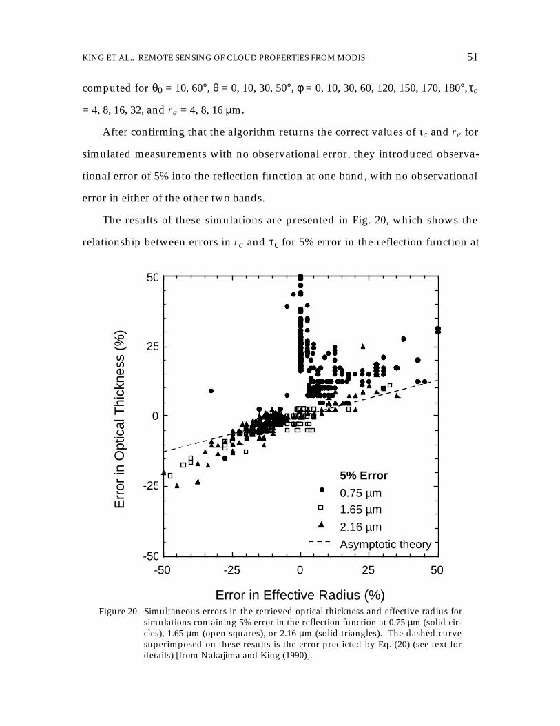
KING ET AL.: REMOTE SENSING OF CLOUD PROPERTIES FROM MODIS 51
computed for θ0 = 10, 60°, θ = 0, 10, 30, 50°, φ = 0, 10, 30, 60, 120, 150, 170, 180°, τc
= 4, 8, 16, 32, and re = 4, 8, 16 µm.
After confirming that the algorithm returns the correct values of τc and re for
simulated measurements with no observational error, they introduced observa-
tional error of 5% into the reflection function at one band, with no observational
error in either of the other two bands.
The results of these simulations are presented in Fig. 20, which shows the
relationship between errors in re and τc for 5% error in the reflection function at
50250-25-50-50
-25
0
25
50
Err
or in
Opt
ical
Thi
ckne
ss (
%)
Error in Effective Radius (%)
5% Error
0.75 µm1.65 µm
2.16 µm
Asymptotic theory
Figure 20. Simultaneous errors in the retrieved optical thickness and effective radius forsimulations containing 5% error in the reflection function at 0.75 µm (solid cir-cles), 1.65 µm (open squares), or 2.16 µm (solid triangles). The dashed curvesuperimposed on these results is the error predicted by Eq. (20) (see text fordetails) [from Nakajima and King (1990)].
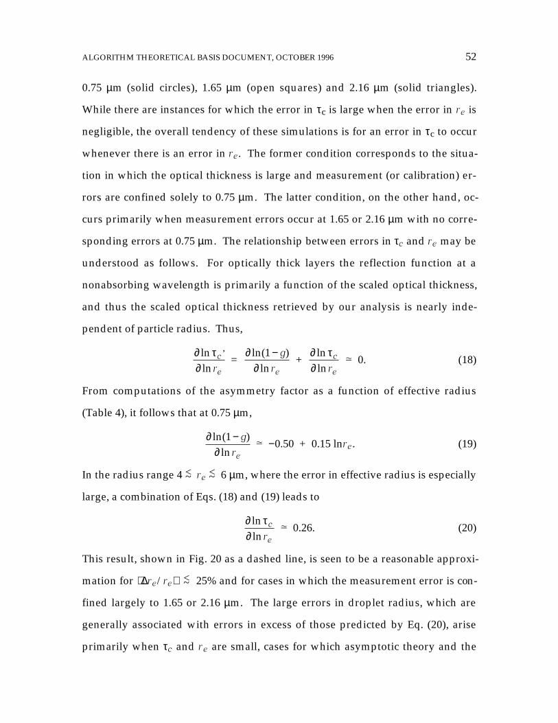
ALGORITHM THEORETICAL BASIS DOCUMENT, OCTOBER 1996 52
0.75 µm (solid circles), 1.65 µm (open squares) and 2.16 µm (solid triangles).
While there are instances for which the error in τc is large when the error in re is
negligible, the overall tendency of these simulations is for an error in τc to occur
whenever there is an error in re. The former condition corresponds to the situa-
tion in which the optical thickness is large and measurement (or calibration) er-
rors are confined solely to 0.75 µm. The latter condition, on the other hand, oc-
curs primarily when measurement errors occur at 1.65 or 2.16 µm with no corre-
sponding errors at 0.75 µm. The relationship between errors in τc and re may be
understood as follows. For optically thick layers the reflection function at a
nonabsorbing wavelength is primarily a function of the scaled optical thickness,
and thus the scaled optical thickness retrieved by our analysis is nearly inde-
pendent of particle radius. Thus,
∂∂lnln
’τc
er =
∂ −∂ln( )
ln1 g
re
+
∂∂
lnln
τc
er · 0. (18)
From computations of the asymmetry factor as a function of effective radius
(Table 4), it follows that at 0.75 µm,
∂ −∂ln( )
ln1 g
re
· −0.50 + 0.15 lnre. (19)
In the radius range 4 <~ re <~ 6 µm, where the error in effective radius is especially
large, a combination of Eqs. (18) and (19) leads to
∂∂
lnln
τc
er · 0.26. (20)
This result, shown in Fig. 20 as a dashed line, is seen to be a reasonable approxi-
mation for ∆ re/re <~ 25% and for cases in which the measurement error is con-
fined largely to 1.65 or 2.16 µm. The large errors in droplet radius, which are
generally associated with errors in excess of those predicted by Eq. (20), arise
primarily when τc and re are small, cases for which asymptotic theory and the
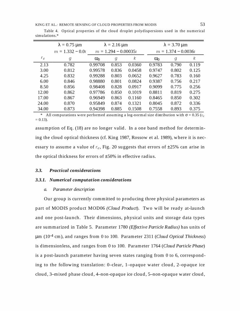
KING ET AL.: REMOTE SENSING OF CLOUD PROPERTIES FROM MODIS 53
assumption of Eq. (18) are no longer valid. In a one band method for determin-
ing the cloud optical thickness (cf. King 1987, Rossow et al. 1989), where it is nec-
essary to assume a value of re, Fig. 20 suggests that errors of ±25% can arise in
the optical thickness for errors of ±50% in effective radius.
3.3. Practical considerations
3.3.1. Numerical computation considerations
a. Parameter description
Our group is currently committed to producing three physical parameters as
part of MODIS product MOD06 (Cloud Product). Two will be ready at-launch
and one post-launch. Their dimensions, physical units and storage data types
are summarized in Table 5. Parameter 1780 (Effective Particle Radius) has units of
µm (10-4 cm), and ranges from 0 to 100. Parameter 2311 (Cloud Optical Thickness)
is dimensionless, and ranges from 0 to 100. Parameter 1764 (Cloud Particle Phase)
is a post-launch parameter having seven states ranging from 0 to 6, correspond-
ing to the following translation: 0–clear, 1–opaque water cloud, 2–opaque ice
cloud, 3–mixed phase cloud, 4–non-opaque ice cloud, 5–non-opaque water cloud,
Table 4. Optical properties of the cloud droplet polydispersions used in the numericalsimulations.*
λ = 0.75 µm λ = 2.16 µm λ = 3.70 µmm = 1.332 − 0.0i m = 1.294 − 0.00035i m = 1.374 − 0.0036i
re g ω0 g k ω0 g k
2.13 0.782 0.99708 0.853 0.0360 0.9783 0.790 0.1193.00 0.812 0.99578 0.836 0.0458 0.9747 0.802 0.1254.25 0.832 0.99288 0.803 0.0652 0.9627 0.783 0.1606.00 0.846 0.98880 0.801 0.0824 0.9387 0.756 0.2178.50 0.856 0.98408 0.828 0.0917 0.9099 0.775 0.256
12.00 0.862 0.97786 0.850 0.1019 0.8811 0.819 0.27517.00 0.867 0.96949 0.863 0.1160 0.8465 0.850 0.30224.00 0.870 0.95849 0.874 0.1321 0.8045 0.872 0.33634.00 0.873 0.94398 0.885 0.1508 0.7558 0.893 0.375
* All computations were performed assuming a log-normal size distribution with σ = 0.35 (ve
= 0.13).

ALGORITHM THEORETICAL BASIS DOCUMENT, OCTOBER 1996 54
and 6–uncertain.
Although reported Effective Particle Radius values are retrieved using the 2.13
µm band in conjunction with a non-absorbing visible band, two other methods of
retrieval are also performed in our algorithm, viz., a 1.64 and a 3.75 µm band re-
trieval method, each in conjunction with a corresponding visible band. Results
from these two alternate methods are expressed in terms of the Effective Particle
Radius Difference, which contains the differences in the retrieved effective radius
between the 1.64 and 2.13 µm methods, and between the 3.75 and 2.13 µm meth-
ods.
The Cloud Mask 1km science data set consists of 1 byte per pixel, and contains
the first byte from Product MOD35 (Cloud Mask). The Quality Assurance 1km
vector consists of 5 bytes per pixel, and consists of (i) the first byte from Product
MOD35 (Cloud Mask), (ii) confidence levels of retrieved parameters, such as cloud
optical thickness, effective radius, and thermodynamic phase, (iii) retrieval proc-
essing path flags, and (iv) input data resource flags. The input data (also referred
to as ancillary data) resource QA flags identify the origins of various input data
sets, whether from NCEP, DAO or other MODIS products. The retrieval proc-
essing path QA flags keeps track of which processing path is taken in the algo-
rithm (either water, ice or mixed phase cloud), what types of atmospheric cor-
Table 5. Summary of MOD06 output parameters produced by Cloud Retrieval Group(based on MOD06 file specification Version 2.0).*
Parameter Name Dimensions* Units Data TypeEffective_Particle_Radius 1354 × 2030 µm integer*2Cloud_Optical_Thickness 1354 × 2030 none integer*2Cloud_Particle_Phase 1354 × 2030 none byteEffective_Particle_Radius_Difference 2 × 1354 × 2030 µm integer*2Cloud_Mask_1km 1354 × 2030 none byteQuality_Assurance_1km 5 × 1354 × 2030 none byteStatistics 20 real*2
* Nominally, a 1 km resolution MODIS granule has 1354 pixels cross track and 2030 detectorlines along track (5 min).

KING ET AL.: REMOTE SENSING OF CLOUD PROPERTIES FROM MODIS 55
rection are used (Rayleigh and/or water vapor), and what band is used for the
optical thickness retrieval. The confidence level QA of a retrieved parameter
(e.g., cloud optical thickness), is three bits long (per pixel): 1 bit is a useful-or-not
useful indicator, immediately followed by 2 bits of confidence levels (0 - 3). The
most updated and complete description of the quality assurance flags can be
found in a separate document (Chu et al. 1997).
Finally, the Statistics array consists of 20 bytes representing statistics com-
puted over the entire MODIS granule. The first 15 values are computed as fol-
lows:
1. Successful retrieval rate;
2. Land cover fraction;
3. Water cover fraction;
4. Snow cover fraction;
5. Cloud cover fraction;
6. Water cloud detected;
7. Ice cloud detected;
8. Mean of water cloud optical thickness;
9. Standard deviation of water cloud optical thickness;
10. Mean of ice cloud optical thickness;
11. Standard deviation of ice cloud optical thickness;
12. Mean of water cloud effective particle radius;
13. Standard deviation of water cloud effective particle radius;
14. Mean of ice cloud effective diameter;
15. Standard deviation of ice cloud effective diameter.
The remaining 5 bytes are currently undefined and are therefore available as
spares for future enhancements.

ALGORITHM THEORETICAL BASIS DOCUMENT, OCTOBER 1996 56
b. Required input data
The MODIS Level-1B calibrated radiance (MOD02) and geolocation fields
(MOD03) are needed by all three retrieved parameters, Cloud Optical Thickness,
Effective Particle Radius, and Cloud Particle Phase. Processed by MCST, the MOD02
product is archived in three separate files, one of which (MOD02_1km) provides
all 36 MODIS bands at effective 1 km spatial resolution, based on integrating the
250 and 500 m pixels according to an approximate point spread function of the
MODIS instrument.
In retrieving the Cloud Optical Thickness and Effective Particle Radius, seven
additional inputs, or ancillary data sets, are required (cf. Table 6). NCEP gridded
analysis and other MODIS data products can be ingested into our retrieval pro-
gram in real-time, whereas DAO data are only available for re-analysis (>72
hours after data acquisition). Except MOD35 (Cloud Mask), all other ancillary
data sets are first handled by ancillary data subroutines and then made available
TABLE 6. Ancillary data sets needed by cloud optical thickness and effective particle radiusretrieval (MOD_PR06OD).
Ancillary Data Categories Data SourcesCloud Top Pressure and Temperature MOD06
DAOCloud Mask MOD35Land Surface Temperature NCEP
DAOMOD11
Sea Surface Temperature NCEPDAO
MOD28Atmosphere Temperature Profile NCEP
DAOMOD07
Atmosphere Moisture Profile NCEPDAO
MOD07Surface Spectral Albedo MOD43
CERES/SARB

KING ET AL.: REMOTE SENSING OF CLOUD PROPERTIES FROM MODIS 57
to the main retrieval program at every pixel that is identified as containing cloud.
In cases where there are multiple data sources, only one is chosen, depending on
the availability of the data source at the time of processing and based on produc-
tion rules set by the Cloud Retrieval Group.
In the post-launch period, the MODIS aerosol product MOD04 will also be
useful for studying aerosol-cloud interactions and their effects on cloud retriev-
als.
c. Data processing path and requirements
The retrieval algorithm outlined in section 3.1 is implemented in practice as
follows:
• set ECS core metadata which contains information about a MODIS prod-
uct that is used for catalog, search, and archival purposes;
• read Cloud Mask information to determine if a given pixel is cloudy or
clear, and determine whether it is a water, ice, or mixed phase cloud;
• call ancillary data subroutines to gather ancillary input data sets;
• read Level-1B data (MOD02_1km) and geolocation fields (MOD03_L1A):
one instrument scan (10 detector lines) of MODIS data at a time for seven
spectral bands (0.645, 0.858, 1.240, 1.640, 2.13, 3.75 and 11.03 µm). Infor-
mation about the viewing geometry (µ, µ0 and φ) is also obtained at this
stage;
• apply atmospheric corrections (Rayleigh, water vapor and other absorbing
gases) to the radiance data;
• perform cloud property retrieval, using either ice or water table look-up
libraries, depending on the thermodynamic phase (cf. Figure 12);
• output results to MOD06 data product.

ALGORITHM THEORETICAL BASIS DOCUMENT, OCTOBER 1996 58
The efficient processing speed of the cloud retrieval code has been improved
by about a factor of 4 since the ß version of the code was first delivered. With the
delivered version 1 code, the MODIS Science Data Support Team (SDST) esti-
mated that it requires about 375 MFLOPS to generate parameters 1780 (Cloud Ef-
fective Particle Radius) and 2311 (Cloud Optical Thickness) with confidence level
values for daily observations over the entire globe (day time only). This includes
a factor of 1.6 for additional time needed for data production, a factor of 0.4 for
cloudy scenes, and a factor of 2 for atmospheric corrections. The version 2 (at-
launch) code has now been developed, and it includes metadata, QA, atmos-
pheric correction, and ancillary files, and hence these scale factors are no longer
required. At the moment, no timing estimates have yet been made for a suffi-
cient number of granules to see what the level-2 sustained (orbital average) proc-
essing rate is expected to be at-launch.
Parameter 1764 (Cloud Particle Phase) is a post-launch parameter. The re-
quired data processing speed is not available at this time, since no prototype
code has yet been developed. However, we estimate that, based on some of our
research code, about 20 MFLOPS should be sufficient.
d. Data storage estimates
The following storage estimates are based on the file specification (Version
2.0) for elements of the MOD06 product produced by the cloud optical depth
process (MOD_PR06OD). This storage is separate and distinct from the storage
requirements of the Menzel and Strabala cloud top properties process
(MOD_PR06CT) and the Gao cirrus detection process (MOD_PR06CD). At 1 km
spatial resolution, the MODIS Science Data Support Team (SDST) estimates 4 ×
108 pixels per day over sun-lit portions of the Earth (2.7 million pixels per gran-
ule multiplied by 144 granules per day). The Cloud Retrieval Group produces

KING ET AL.: REMOTE SENSING OF CLOUD PROPERTIES FROM MODIS 59
day-time only parameters, and the storage requirements for all of these elements
amounts to ~6 GB per day (see below).
Parameter 1764 (Cloud Particle Phase) has values ranging from 0 to 6 and can
be stored as a single byte per pixel. This parameter will be derived for each 1 km
cloudy pixel during the daytime. Thus the data storage required per day, sepa-
rate from the Menzel and Strabala (1997) infrared cloud particle phase algorithm,
is approximately
(4 × 108 pixels) × 1 byte/pixel = 400 Mbytes.
Parameters 1780 (Effective Particle Radius) and 2311 (Cloud Optical Thickness)
have values ranging from 0 to 1000. These parameters are both scaled by a factor
of 10 and stored as 16 bit integers, and are derived for each cloudy 1 km pixel
over the entire globe once per day (day time only). Thus the data storage re-
quired per day is approximately
(4 × 108 pixels) × 2 bytes/pixel = 800 Mbytes
for each of these parameters.
The Effective Particle Radius Difference parameter is also scaled up by a factor
of 10 and stored as 16 bit integers. Since there are two of these difference for
each pixel, the storage requirement for this parameter is
2 × (4 × 108 pixels) × 2 bytes/pixel = 1600 Mbytes.
The Cloud Mask 1km parameter consists of 1 byte per pixel, and hence its
storage requirement is
(4 × 108 pixels) × 1 byte/pixel = 400 Mbytes.
The Quality Assurance 1km parameter requires the largest storage space
among the six output parameters we produce. It consists of 5 bytes per pixel,
and hence its storage requirement is

ALGORITHM THEORETICAL BASIS DOCUMENT, OCTOBER 1996 60
5 × (4 × 108 pixels) × 1 byte/pixel = 2000 Mbytes.
Thus the total storage required for all MOD_PR06OD parameters per day is
approximately
(400 + 800 + 800 + 1600 + 400 + 2000) Mbytes = 6.0 Gbytes,
of which the 400 Mbyte Cloud Particle Phase requirement is only required post-
launch. As a consequence, this parameter is not currently included in the at-
launch file spec, resulting in the at-launch requirement of ~5.6 Gbytes/day.
This estimated figure can easily be reduced by carefully selecting the small-
est data type while still satisfying the precision requirement. The Effective Particle
Radius Difference is currently scaled and stored as 16 bit integers. By definition,
this parameter is the differences in the retrieved effective radius between the 1.64
and 2.13 µm methods, and between the 3.75 and 2.13 µm methods. Presumably
the differences are quite small. A byte data type, rather than a short integer,
might be sufficient. This would result, if implemented, in an 800 Mbyte savings
in storage space per day.
The storage space requirement can be further reduced if a compression algo-
rithm is used. As stated above, all MOD06 data parameters are produced only
over cloudy pixels, and the cloud-free regions are filled with missing values.
Standard compression algorithms work well for this type of data set. HDF re-
lease version 4.1 supports all standard HDF compression algorithms:4 JPEG,
Adaptive Huffman, GZIP “deflation,” (Lempel/Ziv-77 dictionary coder), and
Run-length encoding. In the future, Lempel/Ziv-78 dictionary coding, an arith-
metic coder, and a faster Huffman algorithm may be included. See the HDF 4.1
User’s Guide for more information.
4 The Sdsetcompress routine is only available in C interface at the time of writing.
KING ET AL.: REMOTE SENSING OF CLOUD PROPERTIES FROM MODIS 61
e. Level-3 gridded cloud data
The Level-3 Atmosphere Joint Product (MOD08) algorithm combines pa-
rameters from multiple MODIS atmosphere products including aerosols, cloud
properties, precipitable water, and atmospheric profiles. The integrated atmos-
phere product will be produced on a daily, 8-day and monthly time scale, each of
which will be produced at both an equal angle (1° × 1°) and equal area (~100 km)
spatial scale (cf. Fig. 1). Daily and monthly equal angle grids will be prepared at
launch, with the other products to follow. We will compute statistics separately
for pixels identified as water and ice clouds. Statistics will include the parame-
ters of normal and log-normal distributions in two ways (including and exclud-
ing the effects of our Quality Assurance estimates) and the fraction of ice-cloud
and water-cloud pixels in each grid box. We will also provide histograms of op-
tical thickness and effective particle size, and joint histograms of both optical
thickness and effective particle size with both cloud top temperature and cloud
effective emissivity (the latter two quantities coming from Menzel and Strabala’s
algorithm). After launch we anticipate computing statistics for liquid and ice
water path, derived as W = 2ρτcre/3, where ρ is the density of water.
We have not yet determined the best way to categorize the various quality
control indicators into our joint level-3 product, in part because we lack a com-
plete theoretical understanding of the magnitudes of errors we expect in varying
circumstances. Such assessments, however, will be very important to our ability
to diagnose global indicators of algorithm strengths and weaknesses. Steve Plat-
nick was recently chosen as Principal Investigator under a funding announce-
ment for the EOS Calibration and Validation program, and we anticipate making
substantial use of his results to determine the QA for our Level 2 and Level 3
products. We will produce a separate ATBD that describes the joint level-3 at-

ALGORITHM THEORETICAL BASIS DOCUMENT, OCTOBER 1996 62
mosphere algorithm for MODIS.
3.3.2. Validation
Products from the present algorithm have been tested using MCR data
(Nakajima et al. 1991) as well as from ongoing research projects that utilize MAS
data, as described in Section 2.2. Several field programs offer opportunities for
pre-launch and post-launch MODIS validation through collection and analysis of
observations obtained from the MODIS Airborne Simulator (MAS; King et al.
1996) and High-spectral resolution Interferometer Sounder (HIS; Smith et al.
1995). These field campaigns, principal focus, and MODIS atmosphere group
participants, are summarized in Table 7.TABLE 7. Research & Analysis, and post-launch specific airborne validation campaigns
planned by the MODIS atmosphere group within 3 years of launch of AM-1. This table includesthe primary purpose of the mission as well as the responsible team members and key associates.
Mission Dates Responsible TeamMembers
Primary Purpose
FIRE III May-June 1998 Michael King,Si-Chee Tsay,Steve Platnick,
Steve Ackerman
arctic stratus cloudsover sea ice
MODIS-specific validation ca m paigns
ARM-2 March 1999 Michael King,Si-Chee Tsay,Steve Platnick,
Steve Ackerman
periodic flights over theNSA ARM site withMAS & HIS
California July 1999December 1999
Michael King,Steve Platnick, Si-
Chee Tsay
marine stratocumulus(July) and valley fog(December)
KalahariDesert
August-September 1999
Michael King,Yoram Kaufman,
Si-Chee Tsay,Steve Platnick,Didier Tanré,
Lorraine Remer
smoke, clouds and ra-diation from biomassburning in the Savan-nah; marine stratocu-mulus off Namibian de-sert; surface BRDF

KING ET AL.: REMOTE SENSING OF CLOUD PROPERTIES FROM MODIS 63
In addition to these ER-2 field campaigns, which often include the Cloud Li-
dar System (CLS; Spinhirne et al. 1989) for verifying cloud top altitude and
multi-layer clouds, the University of Washington CV-580, with the Cloud Ab-
sorption Radiometer (CAR; King et al. 1986) and extensive in situ cloud micro-
physics (liquid water content, effective radius, cloud drop size distribution),
aerosol properties (size distribution, scattering and absorption coefficients), and
meteorological sensors, will be used as required.
In addition to these airborne campaigns in which we directly intend to par-
ticipate, we expect to make use of selected ground-based networks (cf. Table 8).
The ground-based measurements will be obtained on a continuous basis as
well as during intensive field experiments. All of these validation opportunities,
as well as intercomparison of data derived from MODIS with other sensors on
AM-1 and other spacecraft, will be discussed in detail below.
Validation will be approached in several ways: (i) collocation with higher
resolution aircraft data, (ii) ground-based and aircraft in situ observations, and
(iii) intercomparisons with other AM-1 instruments. Our validation approach
relies heavily on the sources of the data that were used in the algorithm devel-
TABLE 8. Surface networks that the MODIS atmosphere group plans to utilize, including theprimary purpose of the network and the responsible team members and key associates.
Network Location Responsible TeamMembers
Primary Purpose
AERONET multiple loca-tions: US, Japan,South America,Africa, & Europe
Brent Holben,Yoram Kaufman,
Didier Tanré
aerosol optical thick-ness and columnar sizedistribution
ARM Oklahoma,North Slope ofAlaska, WesternTropical Pacific
Paul Menzel,Si-Chee Tsay
cloud base height(micropulse lidar), tem-perature and moistureprofiles, sky radiance(visible and IR)

ALGORITHM THEORETICAL BASIS DOCUMENT, OCTOBER 1996 64
opment, which consisted primarily of the MAS, HIS, and AVIRIS, a 224 band im-
aging spectrometer from 0.4-2.5 µm with 20 m resolution at nadir (Vane et al.
1993).
Since the spatial resolution of the MAS data is much smaller than that of
MODIS, we plan to use various types of spatial resolution data, such as degraded
MAS data, to test the algorithm during the pre-launch stage. In particular, we
will use the recently upgraded MAS 50 band 12 bit data, together with cloud
mask information from Ackerman et al.’s (1997) algorithm, to test our cloud re-
trieval algorithm.
In the first two years following the launch of EOS AM-1, we anticipate col-
lecting the following data sets for the purpose of validating MODIS algorithms
and data products through direct intercomparisons of MODIS data with in situ
and airborne remote sensing data sets. These campaigns will be EOS-targeted
campaigns of direct relevance to assuring the accuracy of MODIS-derived data
products, and are summarized in Table 9.
The first EOS-targeted campaign after the MODIS launch will be coordinated
with measurements taken at the North Slope Alaska (NSA) ARM site in Barrow,
Alaska, probably in March 1999. The ER-2 with MAS, Scanning HIS, CLS, Air-
MISR, and RAMS will be deployed to synchronize with the MODIS overflight;
the ARM site suite of ground-based measurements (class-sonde, AERI, tower
measurements of temperature and moisture at various elevations, microwave
moisture measurements, lidar and radar observations, whole sky imagers) will
be collected simultaneously. These combined air and ground measurements will
be used to validate MODIS radiance measurements. Results will be used to ad-
just the infrared calibration coefficients as necessary. In addition, the ARM
ground-based measurements can be used to validate geophysical parameters as

KING ET AL.: REMOTE SENSING OF CLOUD PROPERTIES FROM MODIS 65
well. Lidar and radar observations of cloud boundaries over the ARM sites will
be used to validate the presence of a cloud as well as its cloud top pressure alti-
tude. Whole sky imagers are also available at the site, and can be used to com-
pare satellite and ground-based estimates of cloud amount. Finally, optical
depth measurements derived from lidar will aid in specifying the limit of thin
cirrus detection in the cloud mask algorithm.
Once the MODIS is in orbit and returning regular data, we envision two fo-
cused periods of ER-2 overflights, to be coordinated with the EOS AM-1 orbit, in
California (the first one over marine stratocumulus clouds located over the ocean
between Monterey and San Diego in July 1999, and the second over valley fog in
the central valley of California in December 1999). These experiments would
entail ER-2 flights from home base in California (Dryden Flight Research Center),
and would consist, once again, of the MAS and CLS, together with coordinated
TABLE 9. EOS-targeted airborne field campaigns planned by the MODIS atmosphere groupwithin 3 years after the launch of AM-1. This table includes the primary purpose of the campaignas well as the principal sensors to be used, responsible team members and key associates, andprimary purpose.
EOS-TargetedField Campaign
Principal Sensors ResponsibleTeam Members
Primary Purpose
ARM over-flights (SGP &NSA)
MAS, HIS, CLS,AERI, surface li-dar & microwavesensors
Steve Ackerman,Paul Menzel,Bo-Cai Gao,Si-Chee Tsay
mid-latitude cirrusclouds over continents,Arctic stratus over seaice and tundra
California MAS, CLS, Air-MISR
Michael King,Steve Platnick,Si-Chee Tsay
marine stratocumulusand valley fog
KalahariDesert
MAS, AirMISR,CLS, CAR, in situmicrophysics,AERONET
Michael King,Yoram Kaufman,
Si-Chee Tsay,Steve Platnick,Didier Tanré,
Lorraine Remer
smoke, clouds and ra-diation from biomassburning in the Savan-nah; marine stratocu-mulus off Namibian de-sert; surface BRDF

ALGORITHM THEORETICAL BASIS DOCUMENT, OCTOBER 1996 66
underflights by the University of Washington CV-580 with its in situ microphys-
ics probes. This data set, of special interest to Goddard Space Flight Center
(Michael King, Steve Platnick, Si-Chee Tsay), would help to validate the cloud
optical thickness and effective radius between MODIS and the smaller spatial
resolution airborne sensors on the ER-2.
In collaboration with the MODIS Land Group as well as MISR, CERES,
MOPITT, and ASTER, we plan to conduct a 4 week experiment on biomass
burning in the Savannah region of southern Africa (near the Kalahari Desert of
Namibia). Biomass burning occurs in August-September, as in South America,
so we plan to conduct this experiment in August-September 1999, well after the
launch of AM-1. Opportunities to study Namibian marine stratus or other cloud
types may also be available. This experiment, like SCAR-B in 1995, will entail
both the NASA ER-2 aircraft as well as the University of Washington CV-580.
Primary instruments of interest for the ER-2 are the MAS, scanning HIS, CLS,
AirMISR, SSFR, and RAMS. The latter two instruments are to characterize spec-
tral and broadband flux of particular relevance to CERES objectives. As in Brazil
(SCAR-B), we will coordinate the ER-2 with in situ aerosol and chemistry meas-
urements on the CV-580 and overfly numerous AERONET locations in Namibia,
South Africa, Zambia, and Zimbabwe.
Additional post-launch EOS-targeted field campaigns are discussed in the
MODIS Atmospheres Validation Plan (http://eospso.gsfc.nasa.gov/validation/
valplans.html). During the post-launch stage, it is anticipated that one full day of
MODIS data at the 1 km pixel resolution per month will be sufficient for algo-
rithm testing and validation purposes. We only require the spectral bands used
in our algorithm, but would also be interested in selected thermal bands to test
the performance of the cloud mask algorithm. When a major algorithm revision

KING ET AL.: REMOTE SENSING OF CLOUD PROPERTIES FROM MODIS 67
is made, we will require a large data set to test and validate the algorithm. Eight
days of MODIS level-1B data (for the bands given in Table 1) every month will be
sufficient for this purpose.
Algorithm changes will be restrained to occur once per year as needed. We
anticipate assessing the performance of the MODIS algorithms initially by proc-
essing 8 contiguous days per month, as well as specific time periods with valida-
tion experiments of special relevance, as outlined above. After initially looking
at one year’s data, consistency checks, quality assurance flags, validation cam-
paigns, as appropriate, and intercomparisons with other instruments (especially
on AM-1), we will begin whole-scale reprocessing, including every month. This
initial stage may take in excess of one year, during which time the MODIS cali-
bration algorithm will likely undergo additional refinement. Continual refine-
ment of the MODIS “operational” algorithms will largely be conducted at the
Team Member’s SCF as well as at the Team Leader Computing Facility (TLCF),
as many of the algorithms are dependent on results from other algorithms (like
calibration). Only periodically (after say 1.5 years following launch), the first re-
processing at the DAAC will be initiated.
This validation plan represents the thought process of all MODIS atmos-
phere team members, associates, and close colleagues. This group has consider-
able field campaign experience as well as experience with other satellite and sur-
face network data. Putting all MODIS validation schedules together that relate to
the cloud optical thickness, effective radius, and thermodynamic phase algo-
rithms described in this ATBD, we obtain the “master schedule” for MODIS
cloud validation activities, for the focused, field-campaign portion of this plan
(cf. Figure 21).

ALGORITHM THEORETICAL BASIS DOCUMENT, OCTOBER 1996 68
1998 1999 2000
FIRE III
ARM
California
Kalahari DesertAM-1
Research & Analysis Program
MODIS-specific
Figure. 21. ER-2 Validation strategy for the MODIS cloud optical thickness, effective ra-dius, and thermodynamic phase algorithms from 1998 (pre-launch) through2000 (post-launch).
3.3.3. Quality control, diagnostics, and exception handling
The quality control and diagnostics of all post-launch products will be per-
formed based on comparisons with field programs in which related in situ cloud
microphysical data are available. This type of exercise may provide some in-
sights into refining the algorithm. Special cases of missing data, extremely low
sun angles, and the presence of sun glint will be handled separately.
4. Constraints, limitations, and assumptions
There are several assumptions involved in the theoretical development of
cloud particle size and optical thickness retrievals. At the present time, the algo-
rithm is valid for single-layer, liquid water, plane-parallel geometry. Cloudy
pixels that encounter multiple-layer and horizontal inhomogeneity will not be
retrieved correctly. Further developments in the area of detecting multilayer
cloud systems and of correcting for geometrical effects are needed. Also, some
errors are expected to be encountered in retrieved cloud effective particle radius
and optical thickness when ice clouds are present. We currently envision a

KING ET AL.: REMOTE SENSING OF CLOUD PROPERTIES FROM MODIS 69
switch (outlined above) for processing data using a Mie theory phase function
for water clouds and an ice crystal phase function derived for hexagonal crystals
for ice clouds (cf. Fig. 8). Finally, we have yet to determine the upper limit to the
solar zenith angle for which our algorithm can reliably be applied. Unsatisfac-
tory results will no doubt occur when the solar zenith angle θ0 >~ 80°, a switch
that must be set in the operational code. In addition to reduced sensitivity for
large solar zenith angles, there are additional complications arising from in-
creased probability of shadows and finite and 3-dimensional cloud effects. This
is a problem that exists with all such solar cloud reflectance algorithms, and we
currently plan to set this θ 0max = 80°.
5. References
Ackerman, S., K. Strabala, P. Menzel, R. Frey, C. Moeller, L. Gumley, B. Baum, C.
Schaaf, and G. Riggs, 1997: Discriminating Clear-Sky from Cloud with MODIS:
Algorithm Theoretical Basis Document (MOD35). Algorithm Theoretical Basis
Document ATBD-MOD-06, NASA Goddard Space Flight Center, 125 pp.
Arking, A., 1964: Latitudinal distribution of cloud cover from TIROS III photo-
graphs. Science, 143, 569–572.
_____, and J. D. Childs, 1985: Retrieval of cloud cover parameters from multis-
pectral satellite images. J. Climate Appl. Meteor., 24, 322–333.
Bevington, P. R., 1969: Data Reduction and Error Analysis for the Physical Sciences.
McGraw-Hill, 336 pp.
Cess, R, D., G. L. Potter, J. P. Blanchet, G. J. Boer, S. J. Ghan, J. T. Kiehl, H. Le
Treut, Z. X. Li, X. Z. Liang, J. F. B. Mitchell, J. J. Morcrette, D. A. Randall, M.
R. Riches, E. Roeckner, U. Schlese, A. Slingo, K. E. Taylor, W. M. Washing-
ton, R. T. Wetherald and I. Yagai, 1989: Interpretation of cloud-climate feed-

ALGORITHM THEORETICAL BASIS DOCUMENT, OCTOBER 1996 70
back as produced by 14 atmospheric general circulation models. Science, 245,
513–516.
Chu, A., K. Strabala, R. Song, S. Platnick, M. Wang and S. Mattoo, 1997: MODIS
Atmosphere QA Plan, NASA Goddard Space Flight Center, 43 pp.
Cline, A. K., 1974: Scalar- and planar-valued curve fitting using splines under
tension. Comm. Assoc. Comput. Mach., 17, 218–220.
Curran, R. J., H. L. Kyle, L. R. Blaine, J. Smith and T. D. Clem, 1981: Multichan-
nel scanning radiometer for remote sensing cloud physical parameters. Rev.
Sci. Instrum., 52, 1546–1555.
_____, and M. L. C. Wu, 1982: Skylab near-infrared observations of clouds indi-
cating supercooled liquid water droplets. J. Atmos. Sci., 39, 635–647.
DAO, 1996: Algorithm Theoretical Basis Document for Goddard Earth Observing Sys-
tem Data Assimilation System (GEOS DAS) with a focus on Version 2. ATBD-
DAO-01, NASA Goddard Space Flight Center, 131 pp.
Downing, H. D., and D. Williams, 1975: Optical constants of water in the infra-
red. J. Geophys. Res., 80, 1656–1661.
Durkee, P. A., 1989: Observations of aerosol-cloud interactions in satellite-
detected visible and near-infrared radiance. Proc. Symposium on the Role of
Clouds in Atmospheric Chemistry and Global Climate, American Meteorological
Society, Anaheim, CA, 157–160.
Foot, J. S., 1988: Some observations of the optical properties of clouds. I: Strato-
cumulus. Quart. J. Roy. Meteor. Soc., 114, 129–144.
Grainger, R. G., 1990: The calculation of cloud parameters from AVHRR data.
Ph.D. Dissertation, University of Auckland, New Zealand, 188 pp.
Hale, G. M., and M. R. Querry, 1973: Optical constants of water in the 200-nm to
200-µm wavelength region. Appl. Opt., 12, 555–563.

KING ET AL.: REMOTE SENSING OF CLOUD PROPERTIES FROM MODIS 71
Han, Q., W. B. Rossow and A. A. Lacis, 1994: Near-global survey of effective
droplet radius in liquid water clouds using ISCCP data. J. Climate, 7, 465–
497.
_____, W. Rossow, R. Welch, A. White and J. Chou, 1995: Validation of satellite
retrievals of cloud microphysics and liquid water path using observations
from FIRE. J. Atmos. Sci., 52, 4183–4195.
Hansen, J. E., and J. B. Pollack, 1970: Near-infrared light scattering by terrestrial
clouds. J. Atmos. Sci., 27, 265–281.
_____, and L. D. Travis, 1974: Light scattering in planetary atmospheres. Space
Sci. Rev., 16, 527–610.
Irvine, W., M., and J. B. Pollack, 1968: Infrared optical properties of water and ice
spheres. Icarus, 8, 324–360.
Kaufman, Y. J., and T. Nakajima, 1993: Effect of Amazon smoke on cloud micro-
physics and albedo. J. Appl. Meteor., 32, 729–744.
King, M. D., 1981: A method for determining the single scattering albedo of
clouds through observation of the internal scattered radiation field. J. Atmos.
Sci., 38, 2031–204.
_____, 1987: Determination of the scaled optical thickness of clouds from re-
flected solar radiation measurements. J. Atmos. Sci., 44, 1734–1751.
_____, L. F. Radke and P. V. Hobbs, 1990: Determination of the spectral absorp-
tion of solar radiation by marine stratocumulus clouds from airborne meas-
urements within clouds. J. Atmos. Sci., 47, 894–907.
_____, Y. J. Kaufman, W. P. Menzel and D. Tanré, 1992: Remote sensing of cloud,
aerosol and water vapor properties from the Moderate Resolution Imaging
Spectrometer (MODIS). IEEE Trans. Geosci. Remote Sens., 30, 2–27.
_____, M. G. Strange, P. Leone and L. R. Blaine, 1986: Multiwavelength scanning
ALGORITHM THEORETICAL BASIS DOCUMENT, OCTOBER 1996 72
radiometer for airborne measurements of scattered radiation within clouds.
J. Atmos. Oceanic Technol., 3, 513–522.
_____, W. P. Menzel, P. S. Grant, J. S. Myers, G. T. Arnold, S. E. Platnick, L. E.
Gumley, S. C. Tsay, C. C. Moeller, M. Fitzgerald, K. S. Brown and F. G.
Osterwisch, 1996: Airborne scanning spectrometer for remote sensing of
cloud, aerosol, water vapor and surface properties. J. Atmos. Oceanic Technol.,
13, 777–794.
Kou, L, D. Labrie and P. Chylek, 1993: Refractive indices of water and ice in the
0.65- to 2.5-µm spectral range. Appl. Opt., 32, 3531–3540.
Kratz, D. P., 1995: The correlated k-distribution technique as applied to the
AVHRR channels. J. Quant. Spectrosc. Radiat. Transfer, 53, 501–517.
Menzel, W. P., and L. E. Gumley, 1996: MODIS Atmospheric Profile Retrieval Algo-
rithm Theoretical Basis Document. ATBD-MOD-07, NASA Goddard Space
Flight Center, 32 pp.
_____, and K. Strabala, 1997: Cloud Top Properties and Cloud Phase: Algorithm Theo-
retical Basis Document. ATBD-MOD-04, NASA Goddard Space Flight Center,
55 pp.
Mitchell, J. F. B., C. A. Senior and W. J. Ingram, 1989: CO2 and climate: A miss-
ing feedback? Nature, 341, 132–134.
Nakajima, T., and M. Tanaka, 1986: Matrix formulations for the transfer of solar
radiation in a plane-parallel scattering atmosphere. J. Quant. Spectrosc. Ra-
diat. Transfer, 35, 13–21.
_____, and M. D. King, 1990: Determination of the optical thickness and effective
particle radius of clouds from reflected solar radiation measurements. Part I:
Theory. J. Atmos. Sci., 47, 1878–1893.
_____, and _____, 1992: Asymptotic theory for optically thick layers: Application

KING ET AL.: REMOTE SENSING OF CLOUD PROPERTIES FROM MODIS 73
to the discrete ordinates method. Appl. Opt., 31, 7669–7683.
_____, _____, J. D. Spinhirne and L. F. Radke, 1991: Determination of the optical
thickness and effective particle radius of clouds from reflected solar radiation
measurements. Part II: Marine stratocumulus observations. J. Atmos. Sci.,
48, 728–750.
Nakajima, T. Y., and T. Nakajima, 1995: Wide-area determination of cloud mi-
crophysical properties from NOAA AVHRR measurements for FIRE and
ASTEX regions. J. Atmos. Sci., 52, 4043–4059.
Ou, S. C., K. N. Liou, W. M. Gooch, and Y. Takano, 1993: Remote sensing of cir-
rus cloud parameters using Advanced Very High Resolution Radiometer 3.7
and 10.9 µm channels. Appl. Opt., 32, 2171–2180.
Palmer, K. F., and D. Williams, 1974: Optical properties of water in the near in-
frared. J. Opt. Soc. Amer., 64, 1107–1110.
Pilewskie, P., and S. Twomey, 1987: Cloud phase discrimination by reflectance
measurements near 1.6 and 2.2 µm. J. Atmos. Sci., 44, 3419–3420.
Platnick, S., 1991: Remote sensing the susceptibility of cloud albedo to changes
in drop concentration. Ph.D. Dissertation, University of Arizona, Tucson, Ari-
zona, 266 pp.
_____, 1997: The scales of photon transport in cloud remote sensing problems.
IRS 96: Current Problems in Atmospheric Radiation , W. L. Smith and K. Stam-
nes, Eds., A. Deepak Publishing, 206–209.
_____, and S. Twomey, 1994: Determining the susceptibility of cloud albedo to
changes in droplet concentration with the Advanced Very High Resolution
Radiometer. J. Appl. Meteor., 33, 334–347.
_____, and F. P. J. Valero, 1995: A validation study of a satellite cloud retrieval
during ASTEX. J. Atmos. Sci., 52, 2985–3001.

ALGORITHM THEORETICAL BASIS DOCUMENT, OCTOBER 1996 74
Ramanathan, V., 1987: The role of Earth radiation budget studies in climate and
general circulation research. J. Geophys. Res., 92, 4075–4095.
_____, E. J. Pitcher, R. C. Malone and M. L. Blackmon, 1983: The response of a
spectral general circulation model to refinements in radiative processes. J.
Atmos. Sci. 40, 605–630.
_____, R. D. Cess, E. F. Harrison, P. Minnis, B. R. Barkstrom, E. Ahmad and D.
Hartmann, 1989: Cloud-radiative forcing and climate: Results from the
Earth Radiation Budget Experiment. Science, 243, 57–63.
Rawlins, F., and J. S. Foot, 1990: Remotely sensed measurements of stratocumu-
lus properties during FIRE using the C130 aircraft multichannel radiometer.
J. Atmos. Sci., 47, 2488–2503.
Robertson, C. W., and D. Williams, 1971: Lambert absorption coefficients of wa-
ter in the infrared. J. Opt. Soc. Amer., 61, 1316–1320.
Roeckner, E., U. Schlese, J. Biercamp and P. Loewe, 1987: Cloud optical depth
feedbacks and climate modelling. Nature, 329, 138–140.
Rossow, W. B., F. Mosher, E. Kinsella, A. Arking, M. Despois, E. Harrison, P.
Minnis, E. Ruprecht, G. Sèze, C. Simmer and E. Smith, 1985: ISCCP cloud al-
gorithm intercomparison. J. Appl. Meteor., 24, 877–903.
_____, L. C. Gardner and A. A. Lacis, 1989: Global seasonal cloud variations
from satellite radiance measurements. Part I: Sensitivity of analysis. J. Cli-
mate, 2, 419–458.
Slingo, A., 1989: A GCM parameterization for the shortwave radiative properties
of water clouds. J. Atmos. Sci., 46, 1419–1427.
Smith, W. L., H. E. Revercomb, R. O. Knuteson, F. A. Best, R. Dedecker, H. B.
Howell and H. M. Woolf, 1995: Cirrus cloud properties derived from the
high spectral resolution infrared spectrometry during FIRE II. Part I: The

KING ET AL.: REMOTE SENSING OF CLOUD PROPERTIES FROM MODIS 75
High Resolution Interferometer Sounder (HIS) system.. J. Atmos. Sci., 52,
4238–4245.
Spinhirne, J. D., R. Boers and W. D. Hart, 1989: Cloud top liquid water from lidar
observations of marine stratocumulus. J. Appl. Meteor., 28, 81–90.
Stamnes, K., S. C. Tsay, W. Wiscombe and K. Jayaweera, 1988: Numerically sta-
ble algorithm for discrete-ordinate-method radiative transfer in multiple
scattering and emitting layered media. Appl. Opt., 27, 2502–2509.
Stowe, L. L., H. Y. M. Yeh, , T. F. Eck, C. G. Wellemeyer, H. L. Kyle and the Nim-
bus-7 Cloud Data Processing Team, 1989: Nimbus-7 global cloud climatol-
ogy. Part II: First year results. J. Climate, 2, 671–709.
_____, E. P. McClain, R. Carey, P. Pellegrino, G. Gutman, P. Davis, C. Long and S.
Hart, 1991: Global distribution of cloud cover derived from NOAA/AVHRR
operational satellite data. Adv. Space Res., 11, 51–54.
Takano, Y., and K. N. Liou, 1989: Solar radiative transfer in cirrus clouds. Part I:
Single-scattering and optical properties of hexagonal ice crystals. J. Atmos.
Sci., 46, 3–19.
______ , and ______, 1995: Radiative transfer in cirrus clouds. Part III: Light
scattering by irregular ice crystals. J. Atmos. Sci., 52, 819–837.
Tsay, S. C., K. Stamnes and K. Jayaweera, 1989: Radiative energy balance in the
cloudy and hazy Arctic. J. Atmos. Sci., 46, 1002–1018.
______ , ______ and ______ , 1990: Radiative transfer in planetary atmospheres:
Development and verification of a unified model. J. Quant. Spectrosc. Radiat.
Transfer, 43, 133–148.
Twomey, S., and T. Cocks, 1982: Spectral reflectance of clouds in the near-
infrared: Comparison of measurements and calculations. J. Meteor. Soc. Ja-
pan, 60, 583–592.

ALGORITHM THEORETICAL BASIS DOCUMENT, OCTOBER 1996 76
_____. and _____, 1989: Remote sensing of cloud parameters from spectral re-
flectance in the near-infrared. Beitr. Phys. Atmos., 62, 172–179.
van de Hulst, H. C., 1974: The spherical albedo of a planet covered with a homo-
geneous cloud layer. Astron. Astrophys., 35, 209–214.
_____, 1980: Multiple Light Scattering: Tables, Formulas, and Applications, Vols. 1,
Academic Press, New York, 76–82.
Vane, G., R. O. Green, T. G. Chrien, H. T. Enmark, E. G. Hansen, and W. M. Por-
ter, 1993: The Airborne Visible/Infrared Imaging Spectrometer (AVIRIS).
Remote Sens. Environ., 44, 127–143.
Wang, M., and M. D. King, 1997: Correction of Rayleigh scattering effects in
cloud optical thickness retrievals. J. Geophys. Res., 102, 25915–25926.
Wetherald, R. T., and S. Manabe, 1988: Cloud feedback processes in a general
circulation model. J. Atmos. Sci., 45, 1397–1415.
Wu, M. L. C., 1985: Quality of remote sensing measurements of cloud physical
parameters in the Cooperative Convective Precipitation Experiment. J. Geo-
phys. Res., 90, 10551–10562.
Yang, P., and K. N. Liou, 1995: Light scattering by hexagonal ice crystals: Com-
parison of finite difference time domain and geometric optics models. J. Opt.
Soc. Am. A, 12, 162–176.
_____. and _____, 1996a: Finite difference time domain method for light scatter-
ing by small ice crystals in three dimensional space. J. Opt. Soc. Am. A, 13,
2072–2085.
_____. and _____, 1996b: A geometric optics/integral-equation method for light
scattering by nonspherical ice crystals. Appl. Opt., 35, 6568–6584.

KING ET AL.: REMOTE SENSING OF CLOUD PROPERTIES FROM MODIS 77
Appendix. Acronyms
AERI Atmospheric Emitted Radiation Interferometer
AERONET Aerosol Robotic Network
AirMISR Airborne MISR
AM-1 First EOS morning polar-orbiting satellite
ARM Atmospheric Radiation Measurement Program
ARMCAS Arctic Radiation Measurements in Column Atmosphere-surfaceSystem (Beaufort Sea, Alaska, June 1995)
ASTEX Atlantic Stratocumulus Transition Experiment (Azores, June1992)
ASTER Advanced Spaceborne Thermal Emission and Reflection radi-ometer
ATBD Algorithm Theoretical Basis Document
AVHRR Advanced Very High Resolution Radiometer
AVIRIS Airborne Visible/Infrared Imaging Spectrometer
BRDF Bidirectional Reflectance Distribution Function
CAR Cloud Absorption Radiometer
CCN Cloud Condensation Nuclei
CEPEX Central Equatorial Pacific Experiment (Fiji, February-March1993)
CERES Clouds and the Earth’s Radiant Energy System
CLS Cloud Lidar System
COARE Coupled Ocean-Atmosphere Response Experiment
DAAC Distributed Active Archive Center
DAO Data Assimilation Office (NASA Goddard Space Flight Center)
ECS EOSDIS Core System

ALGORITHM THEORETICAL BASIS DOCUMENT, OCTOBER 1996 78
EOS Earth Observing System
EOSDIS EOS Data and Information System
ER-2 Earth Resources high-altitude research aircraft (U2-R)
FIRE First ISCCP Regional Experiment (California, June-July 1987,Beaufort Sea, Alaska, April-June, August 1998)
GCM General Circulation Model
HIS High-spectral resolution Interferometer Sounder
ISCCP International Satellite Cloud Climatology Project
MAS MODIS Airborne Simulator
MAST Monterey Area Ship Tracks Experiment (Monterey and nearbyPacific Ocean, June 1994)
MCR Multispectral Cloud Radiometer
MCST MODIS Characterization Support Team
MISR Multi-angle Imaging SpectroRadiometer
MODIS Moderate Resolution Imaging Spectroradiometer
MOPITT Measurement of Pollution in the Troposphere
NASA National Aeronautics and Space Administration
NCEP National Center for Environmental Prediction (NOAA)
NIR Near-Infrared
NOAA National Oceanic and Atmospheric Administration
NSA North Slope of Alaska
PM-1 First EOS afternoon polar-orbiting satellite
RAMS Radiation Measurement System (Scripps Institution of Ocean-ography)
SARB Surface and Atmosphere Radiation Budget (CERES WorkingGroup)

KING ET AL.: REMOTE SENSING OF CLOUD PROPERTIES FROM MODIS 79
SCAR-A Sulfate, Clouds and Radiation–Atlantic (Delmarva Peninsulaand near-by Atlantic Ocean, July 1993)
SCAR-B Smoke, Clouds and Radiation–Brazil (Brazil, August-September1995)
SCAR-C Smoke, Clouds and Radiation–California (Pacific Northwest,September 1994)
SCF Science Computing Facility
SDST MODIS Science Data Support Team
SGP Southern Great Plains
SSFR Spectral Solar Flux Radiometer (NASA Ames Research Center)
SUCCESS Subsonic Aircraft Contrail and Cloud Effects Special Study(April-May 1996)
SWIR Shortwave Infrared
TIROS Television Infrared Observation Satellite
TLCF Team Leader Computing Facility
TOGA Tropical Ocean Global Atmosphere