global ecological zones for fao forest reporting: 2010 update › 3 › a-ap861e.pdffor fao forest...
TRANSCRIPT

GLOBAL ECOLOGICAL ZONES FOR FAO FOREST REPORTING: 2010 UPdATE
November, 2012
Forest resources Assessment Working Paper 179

FOOD AND AGRICULTURE ORGANIZATION OF THE UNITED NATIONSRome, 2012
Global ecological zones for fao forest reporting:
2010 Update
Forest Resources Assessment Working Paper 179

The designations employed and the presentation of material in this information product do not imply the expression of any opinion whatsoever on the part of the Food and Agriculture Organization of the United Nations (FAO) concerning the legal or development status of any country, territory, city or area or of its authorities, or concerning the delimitation of its frontiers or boundaries. The mention of specific companies or products of manufacturers, whether or not these have been patented, does not imply that these have been endorsed or recommended by FAO in preference to others of a similar nature that are not mentioned.
All rights reserved. FAO encourages the reproduction and dissemination of material in this information product. Non-commercial uses will be authorized free of charge, upon request. Reproduction for resale or other commercial purposes, including educational purposes, may incur fees. Applications for permission to reproduce or disseminate FAO copyright materials, and all queries concerning rights and licences, should be addressed by e-mail to [email protected] or to the Chief, Publishing Policy and Support Branch, Office of Knowledge Exchange, Research and Extension, FAO, Viale delle Terme di Caracalla, 00153 Rome, Italy.

Contents
Acknowledgements vExecutive Summary viAcronyms vii
1. Introduction 11.1 Background 11.2 The GEZ 2000 map 1
2. Methods 62.1 The GEZ 2010 map update. 62.2 Factors influencing the methodology 6
3. Results 83.1 Dataset search 83.2 Datasets used to update map 8
3.2.1 North America 83.2.2 Puerto Rico, US Virgin Islands and Jamaica 103.2.3 Australia 113.2.4 Correcting “No data” polygons 113.2.5 Coastlines and water bodies 11
3.3 FRA Advisory Group meeting 113.4 Classification nomenclature 133.5 Finalizing the map 13
4. Discussion 164.1 The importance of the FAO EZ map 164.2 Methods and datasets 17
4.2.1 Consultative methodology 174.2.2 Notes on some possible source datasets 174.2.3 The connection between climate change initiatives and the GEZ 21
5. Conclusions and recommendations for updating the GEZ map for 2015 225.1 Main recommendations for the 2015 GEZ update 22
APPENDIX 1 account of Datasets available 24
APPENDIX 2 Conversion tables for (1) North america and (2) australia 31
APPENDIX 3 oceania: Tropical and Subtropical Desert Description 38
References 40

BoxesBOX 1 Factors affecting ecological zonation on mountains 10
TablesTABLE 1 Source maps used for the delineation of FAO GEZ 2000 map
(from Simmons (2001) 2TABLE 2 FAO Global Ecological Zoning framework for 2000 (from Simmons (2001) 3TABLE 3 Example of a conversion table from the source map (right) to the GEZ
classification for the 2000 map (left) (Source map: Geographic Distribution of China’s Main Forests (Zheng, 1992) (from Simons (2001)) 4
TABLE 4 Individuals and organizations contacted for input to the FRA 2010 GEZ map. Although attempts were made to contact all scientists involved in the 2000 GEZ map (see Simons (2001) p. 3), not all were successful 9
TABLE 5 Global FRA Advisory Group members in attendance at meeting of 22 June 2011 9TABLE 6 Source maps used for the delineation of FAO GEZ 2010 map 14TABLE 7 FAO Global Ecological Zoning framework for 2010 15TABLE 8 Correlation between climate domains (FAO), climate regions (IPCC)
and EZs (FAO). From: Table 4.1 in IPCC (2006). Forest Land. In 2006 IPCC Guidelines for National Greenhouse Gas Inventories. Vol. 4. Agriculture, Forestry and Other Land Use. Ch. 4. (ed IPCC). IGES Hayama, Japan. 20
figuresFIGURE 1 Köppen-Trewartha map (Trewartha, 1968) 5FIGURE 2 Global Ecological Zones map for FRA 2000. Available online at:
http://www.fao.org/geonetwork/ 5FIGURE 2 Environmental factors contributing to life zone designation. From: Holdridge,
L.R. (1967) Life Zone Ecology. Tropical Science Center, San Jose, Costa Rica 7FIGURE 4 The 2010 GEZ map. GIS data available at: http://www.fao.org/geonetwork/ 15FIGURE 5 IPCC Climate zones according to the IPCC guidelines From IPCC (2006).
Consistent representation of lands. In: 2006 IPCC Guidelines for National Greenhouse Gas Inventories. Vol. 4. Agriculture, Forestry and Other Land Use, Ch. 3. (ed IPCC). IGES, Hayama, Japan 19

v
acknowledgements
This Working Paper is based on a report prepared by FAO consultant Susan Iremonger. FAO is grateful to Dr. Iremonger and to all of the following individuals who assisted with the 2010 update to the FAO Global Ecological Zones:
Brad Smith (USFS) and Zakir Jaffry (CEC) who provided conversion tables for the new data for North America and assisted in finalizing the maps.
Rodney Keenan (Melbourne University) for providing conversion tables for new data for Australia.
Val Kapos and Corinna Ravilious (WCMC)
Zhiliang Zhu and Roger Sayre (USGS)
KD Singh (Forest Survey of India)
Marc Metzger (Edinburgh University)
Antonio Trabucco (Catholic University of Louvain)
Michele Bernardi, Renato Cumani, Adam Gerrand, Erik Lindquist, Remi D’Annunzio, Kenneth MacDicken (FAO)
Emer Crean (Galway-Mayo Institute of Technology)
The FRA Advisory Group also contributed their time and expertise to an early draft of this analysis.
FAO has produced this publication with financial support from the SFM in a Changing Climate Programme funded by the Government of Finland.

vi
Executive Summary
The Global Forest Resources Assessment (FRA) of the Food and Agriculture Organization of the United Nations (FAO) presents global and regional forest data by global ecological zone (GEZ). The GEZ spatial dataset used by FAO has developed over the years from covering only the tropical areas (1990) to the globe (2000). Due to the developments in remote sensing and the compiling of many spatial products relating to climate and land cover between 2000 and 2010, an update to the GEZ 2000 map was commissioned. This took the form of two months’ consultant work spread over May-August 2011, and contributions from other scientists, particularly for North America and Australia.
The new Global Ecological Zone map can be downloaded at: http://foris.fao.org/static/data/fra2010/ecozones2010.jpg
Contact was made with experts who had worked on the 2000 GEZ map as well as with scientists and institutions that had produced or worked with new datasets with potential to contribute to the 2010 map update. A summary of the process for making the 2000 GEZ map and alternatives for update processes were presented to the FRA Advisory Group meeting in June 2011. Proposed activities were very much constrained by the timeframe, which dictated that the map should be finished by the end of July 2011, ready to be used in the statistical analyses of the FAO Global Forest Remote Sensing Survey.
The process agreed during the Advisory Group meeting was adopted, and the following steps were taken for the update:
1. Datasets that were readily convertible to the GEZ classification system were processed and inserted into the GEZ map, replacing old data. These were the areas of North America and Australia.
2. Coastlines and lakes in North America were replaced by new data.3. Coastlines in Australia were replaced through the new dataset.4. Small island polygons that were “No data” in the 2000 map were assigned to an appropriate
GEZ class for this update.5. A resource pool of contact scientists and institutions with experience of creating and using
global and regional climate and ecological zoning datasets was generated.6. A list of 35 global and regional datasets of use for the next update was drafted, and many
of these were downloaded and presented to FAO with this report.
A list of recommendations for the next update of the GEZ map was developed and included in this report. These addressed the timeframe that should be allocated to the update, some possible approaches, scale and resolution issues and specific items relating to particular class types.
Although the changes to the 2000 GEZ map were limited in their scope for this update, any areas that had datasets ready for conversion were included. A great deal of necessary background work that confirmed the unavailability of suitable data was undertaken. This body of work and the datasets gathered will contribute significantly to the success of the next update.

vii
acronyms
CBD Convention on Biological Diversity
CEC Commission on Environmental Cooperation, North America
CRU Climate Research Unit of University of East Anglia
EC Commission of the European Union
ESa European Space Agency EEa European Environment Agency
ETC EEA Topic Centre
EZ Ecological Zone
fao Food and Agriculture Organization of the United Nations
fRa The Global Forest Resources Assessment of FAO
IBRa Interim Biogeographic Regionalisation of Australia IIaSa International Institute for Applied Systems Analysis
IPCC Intergovernmental Panel on Climate Change
GaEZ Global Agro-Ecological Zones GaUL Global Administrative Unit Layer GEo Global Earth Observation GEoSS Global Earth Observation System of Systems GEZ Global Ecological Zones
GIS Geographic Information System
JRC Joint Research Centre of the EC
LET Laboratoire d’Ecologie Terrestre LGP Length of Growing Period NafC North American Forests Commission

viii
RCG Regional Consultative Groups RSS The FAO Global Forest Remote Sensing Survey
SPoT Systeme Pour l’Observation de la Terre
SRTM NASA Shuttle Radar Topography Mission
TNC The Nature Conservancy UCL Catholic University of Louvain, Belgium
UNEP United Nations Environment Programme
USGS United States Geological Survey
WCMC World Conservation Monitoring Centre
WCSD World Commission on Sustainable Development
WSSD World Summit on Sustainable Development

Introduction
1
1. Introduction
1.1 BackgroundThe purpose of creating the FAO Forest Ecological Zones and associated map is to enable the presentation of some of the FAO forest statistics and maps to be shown by a set of classes that have some ecological meaning that can be more generally understood as broad forest types (e.g. tropical rain forests, boreal forests etc.). FAO is also undertaking a Remote Sensing Survey using satellite imagery between 2008 and 2011 to produce a new global forest map and statistics on forest area change (FAO et al., 2009). These activities are a part of the Global Forest Resources Assessment of FAO (FRA) (FAO, 2010).
Conventionally the Food and Agriculture Organization of the United Nations (FAO) reports forest statistics according to political divisions: Nations, Regions and Continents. Expert consultations to the FRA held in Kotka, Finland, provided a mandate for FAO to incorporate indicators of biodiversity into the Assessment (FAO, 2001). In response FAO developed the Global Ecological Zones (GEZ) classification and maps, which were used to present forest statistics including information on forest cover change. An Ecological Zone (EZ) is defined as:
“A zone or area with broad yet relatively homogeneous natural vegetation formations, similar (not necessarily identical) in physiognomy. Boundaries of the EZs approximately coincide with the map of Köppen-Trewartha climatic types, which was based on temperature and rainfall. An exception to this definition are “Mountain systems”, classified as one separate EZ in each Domain and characterized by a high variation in both vegetation formations and climatic conditions caused by large altitude and topographic variation” (Simons, 2001).
There are two main reasons why the GEZ map would need to be updated:
a) there are more accurate source data due to modernisation of resources for mapping; and b) the EZs are changing due to climate change.
For the 1990 FRA only tropical areas were covered by EZ maps (Bellan, 2000). For the 2000 FRA, FAO supported the creation of a new EZ map for the whole globe (Global Ecological Zone map, GEZ) through a process of expert consultation (Iremonger & Cross, 2000; Simons, 2001). In the 10 years between 2000 and 2010 a number of new datasets became available that could influence the delineation and classification of EZs. Additionally, source maps for the 2000 map may have been updated. FAO commissioned the current project to determine the status of these, and examine any new datasets for suitability for inclusion in the GEZ map for the 2010 FRA analyses. To give context to the scope and limitations of the 2010 update, the process used to draft the GEZ 2000 map is outlined below. It is worth noting that although that project was relatively long and went through various stages to reach completion over 3 years, even then the scientists indicated that a more detailed job could have been done with more time and resources (Singh, 2000).
1.2 The geZ 2000 mapAs part of the current project the methodology and logic applied in the drafting of the GEZ 2000 map was revisited. The GEZ 2000 map was made through a process involving a number of stages (FAO, 2001; Simons, 2001). Originally, Ecofloristic Zone maps of Africa, South

Global ecological zones for fAo forest reporting: 2010 Update
2
America and Continental South-East Asia produced by the Laboratoire d’Ecologie Terrestre (LET), Toulouse, France, were converted for use in the 1990 FRA tropical analysis (FAO, 1989, 1993; Lavenu et al., 1988; Sharma, 1986, 1988). The possibility of making an EZ map of global extent for the 2000 FRA was investigated through pilot projects and case studies (Bellan, 2000; Iremonger & Cross, 2000; Preto, 1998; Simons et al., 1999; Zhu, 1997). One study reviewed existing global and regional maps that could be used as resources for the regional or global mapping, including a number of climate and potential vegetation classifications (Simons et al., 1999). Others investigated the practical approaches and methodologies that could be used (Preto, 1998; Singh, 2000; Zhu, 1997). The conclusions from pilot studies were that there was no possibility of creating a completely new EZ map and database in time to use in the 2000 FRA, but that existing data and systems should be used (FAO, 2001; Singh, 2000). A system was proposed that involved adapting maps already in existence, and combining them to produce a comprehensive world coverage with a single classification scheme.
TaBLe 1Source maps used for the delineation of Fao geZ 2000 map (from Simmons (2001))
region name of map Scale projection Thematic information / classification criteria
Canada and Mexico Ecological regions of North America (CEC, 1997)
1: 10 million Lambert Azimuthal Equal Area
Holistic classification system based on climate, soils, landform, vegetation and also land use. Hierarchic system:15 Level I ecological regions and 52 Level II regions.
USA Ecoregions of the USA (Bailey, 1994)
1: 7.5 million Lambert Azimuthal Equal Area
Classification based on Köppen climate system: broad domains equivalent to climate groups, subdivided into divisions approximately equivalent to climate types.
Central America National Holdridge Life zone maps transformed to a regional base map
Various scalesBase map at1: 1.5 million
Various Holdrige Life Zones are defined using the parameters (bio)temperature, rainfall and evapotranspiration. See (Simons, 2001) p. 60 for individual map details.
South America, Africa, Tropical Asia
Ecofloristic zones maps (Bellan, 2000)
1: 5 million Lat-Long 28 groups of ecofloristic zones are defined, based on climate, vegetation physiognomy and physiography, i.e. altitude. The EFZ identifies the most detailed ecological units, based on the additional criteria of flora and geographic location.
Middle East Vegetation map of the Mediterranean zone (UNESCO & FAO, 1969)
1: 5 million Distribution of potential vegetation formations in relation to climate. The various formations are distinguished mainly on basis of physiognomy.
Europe General Map of the Natural Vegetation of Europe. (Bohn et al., 2000)
1: 10 million Equidistant_Conic
Distribution of potential natural plant communities corresponding to the actual climate and edaphic conditions. At broadest level 19 vegetation formations defined, of which 14 zonal and 5 azonal formations.
Former Soviet Union Vegetation map of the USSR (Isachenko et al., 1990)
1: 4 million Lambert Azimuthal Equal Area
Distribution of broad vegetation formations related to climate, altitude and also current land use. 133 vegetation classes are aggregated into 13 categories of vegetation
China Geographic Distribution of China’s Main Forests (Zheng, 1992)
Main aim to identify and map China’s forest vegetation A hierarchic classification is used based on climate and distribution of forest types and tree species. 27 Forest Divisions are mapped.
Australia Interim Biogeographic Regionalisation for Australia (Thackway & Cresswell, 1995)
1: 15 million Albers Equal Area
Major attributes to define biogeographic regions are: climate, lithology/geology, landform, vegetation, flora and fauna and land use. A total of 80 IBRA regions have been mapped.
Caribbean, Mongolia, Korea’s, Japan, New Zealand, Pacific Isl.
Terrestrial Ecoregions of the World (WWF, 2000)
1:30 million Lat-Long Ecoregions are defined by shared ecological features, climate and plant and animal communities. Main use is for biodiversity conservation.
Introduction
3
Case studies were an important test for the methodology because they showed that maps from different sources using different classifications of ecoregions or EZs could be made into one coherent map by experts using conversion tables. For each source map a conversion table converted the classes in the source dataset to the proposed GEZ classification scheme (see below).
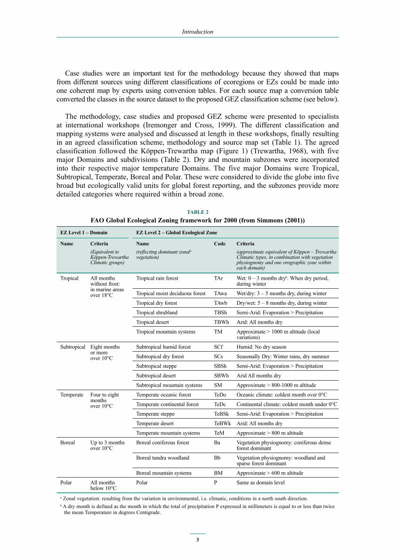
The methodology, case studies and proposed GEZ scheme were presented to specialists at international workshops (Iremonger and Cross, 1999). The different classification and mapping systems were analysed and discussed at length in these workshops, finally resulting in an agreed classification scheme, methodology and source map set (Table 1). The agreed classification followed the Köppen-Trewartha map (Figure 1) (Trewartha, 1968), with five major Domains and subdivisions (Table 2). Dry and mountain subzones were incorporated into their respective major temperature Domains. The five major Domains were Tropical, Subtropical, Temperate, Boreal and Polar. These were considered to divide the globe into five broad but ecologically valid units for global forest reporting, and the subzones provide more detailed categories where required within a broad zone.
TaBLe 2Fao global ecological Zoning framework for 2000 (from Simmons (2001))
eZ Level 1 – domain eZ Level 2 – global ecological Zone
name criteria(Equivalent to Köppen-Trewartha Climatic groups)
name(reflecting dominant zonala vegetation)
code criteria(approximate equivalent of Köppen – Trewartha Climatic types, in combination with vegetation physiognomy and one orographic zone within each domain)
Tropical All months without frost: in marine areas over 18°C
Tropical rain forest TAr Wet: 0 – 3 months dryb. When dry period, during winter
Tropical moist deciduous forest TAwa Wet/dry: 3 – 5 months dry, during winter
Tropical dry forest TAwb Dry/wet: 5 – 8 months dry, during winter
Tropical shrubland TBSh Semi-Arid: Evaporation > Precipitation
Tropical desert TBWh Arid: All months dry
Tropical mountain systems TM Approximate > 1000 m altitude (local variations)
Subtropical Eight months or more over 10°C
Subtropical humid forest SCf Humid: No dry season
Subtropical dry forest SCs Seasonally Dry: Winter rains, dry summer
Subtropical steppe SBSh Semi-Arid: Evaporation > Precipitation
Subtropical desert SBWh Arid All months dry
Subtropical mountain systems SM Approximate > 800-1000 m altitude
Temperate Four to eight months over 10°C
Temperate oceanic forest TeDo Oceanic climate: coldest month over 0°C
Temperate continental forest TeDc Continental climate: coldest month under 0°C
Temperate steppe TeBSk Semi-Arid: Evaporation > Precipitation
Temperate desert TeBWk Arid: All months dry
Temperate mountain systems TeM Approximate > 800 m altitude
Boreal Up to 3 months over 10°C
Boreal coniferous forest Ba Vegetation physiognomy: coniferous dense forest dominant
Boreal tundra woodland Bb Vegetation physiognomy: woodland and sparse forest dominant
Boreal mountain systems BM Approximate > 600 m altitude
Polar All months below 10°C
Polar P Same as domain level
a Zonal vegetation: resulting from the variation in environmental, i.e. climatic, conditions in a north south direction.b A dry month is defined as the month in which the total of precipitation P expressed in millimeters is equal to or less than twice
the mean Temperature in degrees Centigrade.

Global ecological zones for fAo forest reporting: 2010 Update
4
Regional and national specialists converted the different source maps to the GEZ system using tables such as that in Table 3, and finally a global map was compiled (Figure 2). This was accompanied by a report that contained the conversion tables for the source maps and descriptions of the GEZs for each major region of the globe (Simons 2001). The project duration was about three years, from 1998 to 2001. This latest update has been a lot shorter and carried out over four months from May to August of 2011. The main aim of the update was not to completely revise the system, but just to review new datasets and include them where appropriate for FRA 2010 and make recommendations on revisions for the GEZ for FRA 2015.
The new Global Ecological Zone map can be downloaded at: http://foris.fao.org/static/data/fra2010/ecozones2010.jpg
TaBLe 3example of a conversion table from the source map (right) to the geZ classification for the 2000 map
(left) (Source map: geographic distribution of china’s main Forests (Zheng, 1992) (from Simons (2001))
Fao system corresponding source class: geographic divisions of china’s main forests
domain geZ
Tropical TAwa (21) Leizhou Peninsula Division(22) Hainan Island Division
TM (23) Southern Yunnan Division
Subtropical SCf (13) Middle-to-Lower Changjiang Alluvial Plain Division(15) South of Changjiang Low Mountain Division(16) Sichuan Basin Division(18) Taiwan Division(19) South China Hilly Division
SM (14) Qinling Range and Dabashan Mountain Division(17) Yunnan Plateau Division(20) Western Guangxi and Central-Southern Yunnan DivisionParts of Central Temperate zone, Interior dry Region
Temperate TeDc (2) Eastern Mountain Division(4) Liaodong Peninsula and Shandong Peninsula Division(5) Huanghuaihai Coastal Plain Division
TeBSk (3) Western Plain DivisionParts of Central Temperate zone, Interior dry Region
TeBWk Parts of Central Temperate zone, Interior dry Region
TeM (6) North China Middle-to-Low Mountain Division(7) The Loess Plateau Division(8) Southern Gansu and Northern Sichuan Division (9) Eastern Kangding Division (10) Western Kangding Division(11) Southern Sichuan and Northwestern Yunnan Division(12) Southeastern Tibet Division(24) Altai Mountain Division(25) Tianshan Mountain Division(26) Qilianshan Mountain Division Parts of Central Temperate zone, Interior dry Region
Boreal Ba (1) Daxinganling Division

Introduction
5
FIgure 1köppen-Trewartha map (Trewartha, 1968)
FIgure 2global ecological Zones map for Fra 2000. available online at: http://www.fao.org/geonetwork/

Global ecological zones for fAo forest reporting: 2010 Update
6
2. methods
2.1 The geZ 2010 map updaTeFAO recognised that there have been significant updates in spatial data since the previous GEZ work in 2001. A consultant was commissioned to work with FAO to review new datasets, compile an updated GEZ map version for FRA 2010 and make recommendations for FRA 2015 EZ work. The scope of this work was limited due to time and resource constraints (two months’ consultant work between May and August 2011) and so it was not possible to do an intensive international consultation phase in this update. The FRA Advisory Group in June 2011, however, did contain experts with a wide range of global experience and was used to confirm a protocol for the current update and to produce recommendations for further updates.
As part of the baseline work before the Advisory Group meeting, requests for input to the update were sent to individuals and organizations involved in the 2000 map and others involved in the production of relevant global data since 2000. Internet searches were carried out to identify any global products that could contribute to the definition of the EZs for the new map.
2.2 FacTorS InFLuencIng The meThodoLogyThere were a number of factors that interacted to influence the characteristics of the 2000 GEZ map. An obvious one was that it was the product of experts who had worked for many years in the fields of ecological zoning, actual and potential vegetation mapping and forest mapping. The experts contributed their considerable experience and knowledge to the map, giving it credibility and acceptability. Another was that some source maps were the base for national reporting of forest statistics to FAO. These maps already had “ecoregions” or “bioregions” delimited in them that formed the reporting units. In these cases attempts were made not to have to split the ecoregional polygons for the GEZ map: to assign each as an entity to a particular EZ. This can give rise to somewhat peculiar shapes to the GEZ divisions: but it is a practical framework by which to draw boundaries and used in other maps for international reporting (EEA Pan-European Biogeographical map, see Appendix 1).
The alternative route for a new FAO GEZ map would be to determine EZs independently of the national or regional maps by using a more objective approach. This can be done by relying solely on climate and altitude data to delimit zones: not including the experience of experts using maps created by also taking potential vegetation, and vegetation classification, into account. This was not the chosen method for the 2000 GEZ map, but as national reporting, and mapping, becomes more automated, this route may gain favour. There may be models developed that may be useful such as the Environmental Stratification of Europe (Metzger et al., 2005) or those used for the IPCC processes. These automated or semi-automated methods can be used to develop agro-climatic classifications such as the Global Agro-Ecological Zones Database (GAEZ) (Fischer et al., 2002; Hutchinson et al., 2005) and can have advantages such as enabling crop production or other modelling. However, they should be approached with caution, as climate data themselves are interpolated from weather station data which are often sparsely located and irregular. The datasets are therefore an estimate of climate, and this can introduce errors. The natural vegetation of an area, on the other hand, has been influenced by a long history of the climate of the area, as well as other environmental factors, and is a confirmed indicator of an ecological zone. Indeed climate classifications were originally

7
Methods
based on major vegetation types (Bailey, 1989; Köppen, 1931; Singh, 2000; Walter, 1973). Figure 3 gives an impression of the relationships between climate and potential vegetation. These zones and classes are similar to the GEZ but do not match exactly as the GEZ were developed by experts with a focus on forest classification.
FIgure 3environmental factors contributing to life zone designation. From: holdridge, L.r. (1967)
Life Zone ecology. Tropical Science center, San Jose, costa rica

Global ecological zones for fAo forest reporting: 2010 Update
8
3. results
3.1 daTaSeT SearchThe individuals and organizations contacted included those involved in drafting the 2000 map, FRA Advisory Group members and others that had used or produced relevant data since 2000 (Tables 4 and 5). Among those who responded only North America and Australia had definite new source data that could be used for the update. Enthusiastic input both from the Advisory Group and from other scientists was very gratefully accepted and is acknowledged here. Datasets actually used for the update are described in Section 3.2. Other data were identified as possible source material (Appendix 1): these were all of very high quality. Most had been created since 2000, were drafted by recognised teams of scientists and had gained acceptance by being used as source data in published literature and/or international processes. However, for the purposes of updating the GEZ map most of these were unsuitable in one way or another, as outlined below. Some of the datasets are discussed in Section 4.2.
1. Datasets depicting actual (not potential) vegetation cover/land cover were problematic in that the depiction of EZs should not be influenced by current land cover characteristics, except where that has not been influenced in any major way by human activity.
2. Datasets with a significant number of polygons that showed no relation to the currently-defined GEZ boundaries were problematic in that there was a mismatch between the fundamental framework of their classification criteria and that of the GEZ. This is not to say that they were not good datasets: just that the criteria for zoning were different to those of the FAO GEZ map.
3. Relating in particular to new climate data, excellent new data were found that could potentially be used to refine the GEZ boundaries. However, climates portrayed in these data did not follow the same system as that of the Köppen-Trewartha map. As this forms the base of the GEZ classification, the new data could not be used without significant re-working. The timeframe for this project did not allow for that.
4. Consideration was given to re-drawing the boundaries of the Mountain systems polygons, as there were excellent new elevation data available (SRTM, see Appendix 1). Approximate lowest altitude boundaries were given in the mountain class descriptions for the 2000 GEZ (Simons, 2001). However, using a simple altitude cutoff to depict a mountain systems zone within each Domain would not be good ecological practice, as other factors besides elevation influence the ecology of land cover on a mountain (e.g. size of mountain, local topography, surrounding landform) (Box 1). For this reason the boundaries of the Mountain systems polygons were maintained as in the 2000 GEZ map, as these were determined by regional specialists.
3.2 daTaSeTS uSed To updaTe map3.2.1 north americaIn May 2010 an agreement (independent of the GEZ update process) was made between Canada, USA and Mexico at the annual meeting of the FAO/NAFC (North American Forests Commission) Inventory and Monitoring Working Group meeting in Guadalajara, Mexico to use the Ecological Regions of North America (Commission on Environmental Cooperation, CEC) as the base map for the North American Database Project (FAO NAFC, 2010). This provides data for FRA tables 1-4 and 6-8 by ecoregion for North America based on national

9
Results
TaBLe 4Individuals and organizations contacted for input to the Fra 2010 geZ map.
although attempts were made to contact all scientists involved in the 2000 geZ map (see Simons (2001) p. 3), not all were successful
Scientist Institution dataset
Achard, Frederic EC JRC Europe maps
Brokaw, Nicholas University of Puerto Rico Puerto Rico map
Chai, Shauna Jamaica Conservation and Development Trust Jamaica data
Davis, Robert World Bank FAO GEZ
Du, Zheng Chinese Academy of Sciences China map
Gonzalez, Patrick University of California, Berkeley MC1 DGVM
Hennekens, Stephan Wageningen University Natural Vegetation of Europe map (Bohn and Golub)
Hiederer, Roland EC JRC Global climate and EZ maps
Hijmans, Robert University of California, Davis WorldClim
Jaffry, Zakir CEC North America dataset
Leemans, Rik Wageningen University Holdridge life zones
Metzger, Marc University of Edinburgh Environmental Stratification of Europe. Global Environmental Stratification
Nielson, Ron Oregon State University MAPSS, MC1
Prentice, Colin Macquarie University BIOME models
Ramankutty, Navin Potsdam Institute for Climate Impact Research Global potential vegetation map
Richard, Dominique EEA ETC-Biodiversity EEA Biogeographical regions and other Europe maps
Sayre, Roger USGS GEOSS Ecosystems
Shvidenko, Anatoly IIASA Russia map
Singh, Karn Deo Forest Survey of India FAO GEZ
Smith, Brad US Forest Service North America EZ map
Trabucco, Antonio Université Catholique de Louvain PET and Aridity Index
Zhu, Zhiliang USGS EDC FAO GEZ
TaBLe 5global Fra advisory group members in attendance at meeting of 22 June 2011
Scientist Institution
Bahamondez, Carlos INFOR, Chile
Belward, Alan JRC, Italy
Christophersen, Tim CBD, Canada
Gueye, Souleyman DEFCS, Senegal
Mansur, Eduardo ITTO, Japan
Kapos, Valerie UNEP-WCMC, UK
Keenan, Rodney U. Melbourne, Australia
Korhonen, Kari Metlä, Finland
Maginnis, Stewart IUCN, Switzerland
Mariano, Angelo Corpo Forestale, Italy
Michalak, Roman UNECE, Switzerland
Veloso de Freitas, Joberto SFB, Brazil
Zhang, Min Dept of Forest Resources, China

Global ecological zones for fAo forest reporting: 2010 Update
10
forest inventory (NFI) data. The source maps for Mexico and Canada in the 2000 GEZ map were from this database, but the map for USA was from a different source. For the current update of the GEZ map the USFS produced a conversion table from the CEC system to the GEZ scheme for USA. Together with the CEC a new GEZ map for the entire area of North America was produced according to Appendix 2.
The EZ polygons of the new North America data were matched with those of Central America by merging polygons, smoothing lines and cleaning up slivers to make a unified dataset.
3.2.2 puerto rico, uS Virgin Islands and JamaicaThe new North American data (above) assigned Puerto Rico and the US Virgin Islands entirely to the class Tropical mountain system. A review of these areas in the 2000 GEZ map showed that there was more detail in the older dataset. A comparison with two maps of Puerto Rico (Land cover of the Commonwealth of Puerto Rico (Helmer et al., 2002) and Life Zones of Puerto Rico (updated from (Ewel & Whitmore, 1973)) indicated that the 2000 GEZ map was more accurate for these islands, but that it did not include the Tropical mountain systems polygons, which were erroneous. The solution was to leave the territories as they were in 2000 but to also digitise the Lower montane polygons from the Life Zones of Puerto Rico map, and include them in the 2010 map.
BOx 1Factors affecting ecological zonation on mountains
According to the report issued with the FAO GEZ 2000 map:
“Mountain systems are defined as zones/areas that have a distinctly different vegetation (and climate) than the surrounding lowlands at a given latitude. Mountain vegetation is usually lower [shorter] and the floristic composition is different (with generally fewer species). Additional components to define mountain systems are altitude and steepness of slopes. It is difficult to select specific altitudinal thresholds for defining mountain systems also as [because] the changes in vegetation are often gradual, however they are usually at around 1000 - 1200 meter in the tropics and decrease with higher latitudes.”
The approximate altitude line for defining the Mountain systems category in that map varied according to the Major Domain, thus for Tropical was 1000m, Subtropical 1000-800, Temperate 800m and Boreal 600m. However, the Mountain systems zones were drawn using boundaries of vegetation changes in regional and national maps, so the boundaries tend to follow the vegetation mapping more than the altitudinal levels.
Although vegetation changes with altitude, other topographical characteristics also influence the vegetation. On smaller mountains the bioclimatic vegetation zonation is compressed as compared with larger mountains (Crawford, 2008). This is known as the Massenerhebung effect (mass elevation effect): altitude has less effect on vegetation on larger mountains than on smaller ones (Crawford, 2008; Grubb, 1971). The difference is most noticeable where large mountains are massed together. The three main tropical forest types found on wet tropical mountains are: Lowland rainforest, Lower montane forest and Upper montane forest (Grubb, 1971). They are defined by the plant associations and altitudinal limits, but these limits vary with the size of the mountain. On small, isolated mountains and outlying ridges of major ranges, the upper limit of lowland rain forest is about 700−900 m and that of the lower montane rain forest about 1,200−1,600 m, whereas on the main ridges of major ranges the limits are higher, approximately 1,200−1,500 m and 1,800−2,300 m, respectively (Grubb, 1971).

11
Results
An examination of the other Greater Antilles showed that the mountains in Jamaica had also been overlooked in the 2000 version of the GEZ map. A map showing land cover on Jamaican mountains was used to provide a very rough guide to the delineation of Tropical mountain system polygons for that island (Muchoney et al., 1994). As the GEZ maps are not recommended for use at scales larger than 1:10Million the accuracy of these polygons was adequate.
3.2.3 australiaThe Interim Biogeographic Regionalisation of Australia (IBRA) was the source dataset for that area in the 2000 GEZ map. The version of the dataset in 2000 was updated and the version available in 2011 was 6.1. A new conversion table was made at the University of Melbourne (Appendix 2) and a new version of the GEZ map for Australia was produced.
The changes are considered to be refinements and improvements for the GEZ 2000 map and include the following: The class of Tropical desert was included for parts of Northern Australia in the 2010 update although it was not in the GEZ 2000 because it is now thought to better reflect the climatic and vegetation boundaries. Reclassification of the area south of the Gulf of Carpentaria better reflects the distribution of forests in that region and is more consistent with the climate classification. The only other major difference is the area north of the Eyre Peninsula in South Australia. This also fits the climate classification better (Keenan, pers. comm.).
3.2.4 correcting “no data” polygonsA number (130) of small islands were coded as “No data” in the 2000 GEZ map. These were assigned to a GEZ class during the current update. The main datasets for determining their class were the Köppen-Trewartha climate map, the global TNC/WWF ecoregions map (TNC, 2009) and the WorldClim altitude data (see Appendix 1).
3.2.5 coastlines and water bodiesCoastlines and water bodies in the GEZ 2000 map were derived from Environmental Systems Research Institute’s Arc World 1994. For the current update these were left as they were with the following exceptions:
Coastlines in North America transferred with new CEC dataset (see above), which were designed for use at scales up to 1:1Million. Lakes for that area were cut out from the land area using the Global Lakes and Wetlands Database (GLWD 1), also 1:1M resolution, using a minimum size limit of >2,500 km2.
The Australian coastline was from IBRA version 6.1.
The “water” class (lakes) in the 2000 GEZ map were cut out of the current map. As a result all the inland water bodies appear as holes in the 2010 GEZ dataset, and there is no “water” class.
3.3 Fra adVISory group meeTIngFAO implements the Global Forest Resources Assessment (FRA) on request of its member countries. To implement this mandate, FAO regularly seeks broad guidance from a large number of national and international experts and agencies. The FRA Advisory Group is made up of approximately 20 members with a wide variety of geographic and subject expertise. (http://www.fao.org/forestry/fra/ag/en/). A FRA Advisory Group meeting was held in Rome in June 2011 attended by many of the members (see list in Table 5) and the opportunity was taken to discuss the GEZ update work.

Global ecological zones for fAo forest reporting: 2010 Update
12
This meeting was used to get expert input on the following specific subjects, and for general guidance regarding the acceptability of the GEZ system for forest reporting, and the future of the map. The following subjects were addressed:
1. The acceptability of the classification system of the GEZ map, in terms of any changes required.2. The suitability of the Environmental Stratification of Europe database as a new source for
the GEZ map.3. The suitability of the GEOSS Ecosystems of Africa map as a new source for the GEZ map.4. The methodology for this update, taking practicalities (timeframe, financial and human
resources) into account.5. The future of the FAO EZ map, considering other global processes and information needs.
The main outcomes of this meeting were:
1. The GEZ classification system worked well, following both climate and potential vegetation characteristics of the globe. The five major Domains (Tropical, Subtropical, Temperate, Boreal and Polar) were considered to divide the globe into five ecologically valid units for reporting, and the subzones gave substance to these divisions. The Group recommended that the nomenclature of the zones be examined further by specialists during a future update. Implications of making a change to the class name “Tropical moist deciduous forests” should be examined to consider dropping the word “deciduous” to recognise that some areas of predominantly evergreen forest are within these zones.
2. The Environmental Stratification of Europe database was examined but was found to be inappropriate for use in the current update. The classification and polygons were not found to relate easily to the divisions in the 2000 EZ map. Some participants found the units in the map did not adequately reflect existing vegetation units on the ground. During a future update it was possible that this dataset could be examined in conjunction with other datasets, and that manipulation of the classes and polygons may achieve a good result. The European Environment Agency (EEA) Pan-European Biogeographical regions was suggested as a possible more suitable source for the new polygons, although this would also need to be tested for conversion also by a focus team. It would require a trained group and a reasonable period of time to carry out a conversion of these datasets for the FAO map, and the Group suggested examination of these for the next update as part of FRA 2015.
3. The Group considered that for a number of reasons it was difficult, if not impossible, to use the GEOSS map of Africa for the FRA EZ update. A number of the classes presented complex problems to convert to the FAO EZ classes. It appeared the scales of input data to the GEOSS map were not uniform, and perhaps there were raster and vector origins in the dataset. A proper update for the Africa part of the EZ map should involve a focus team of regional experts who would review and select the best data to replace what is in the 2000 EZ map.
4. Considering the time constraints of the current update and the outcomes of the sessions on Europe and Africa, the current update was considered to be confined to including new linework for North America using the updated CEC map and for Australia using the updated IBRA map. Map datasets for other regions were not suitable, generally because they showed actual rather than potential vegetation (e.g. GLC2000, GEOSS Ecosystems of South America), or were too difficult to convert to the EZ classification without regional experts (see items 2 and 3, above).
5. The suggested procedure for Asia was generally to keep the map as it was in 2000. However, as the zoning in China did not have a lot of detail, and efforts had already been started to get new data for that area, it was recommended to pursue this and include new data if possible for this update.

13
Results
6. Updated boundaries for the mountain zones could possibly come from new digital elevation data. However, considering that there are other effects on EZs on mountains other than altitude (see Box 1), the use of altitudinal cutoff lines to define mountain zones could only be used as a guide. The Group recommended this aspect of the map be checked by regional experts during the next update.
7. The Group emphasised that to maintain credibility and acceptability across nations and regions the consultative method for making the map should be maintained. It recommended that a wider-reaching overhaul should take place as part of FRA 2015, and that as this would take a significant amount of time it should start as soon as possible. It was agreed that major changes, including new models and data sets could be implemented for FRA 2015.
8. The opportunity for doing a user-survey was discussed briefly and the group recommended that it should be considered as part of FRA 2015 work. Time was not available to do a proper survey for the current update, however, an offer by KD Singh to initiate such a survey was an option that was noted. This would involve testing the GEZ classification with forest data from India.
9. The question of whether the dataset should evolve with climate change should be discussed in depth during the next update. The FAO GEZ 2000 appears in IPCC documents as a scheme for dividing the globe into ecological units, and may be used for calculating carbon budgets. FAO should work with IPCC on the conceptual aspects of the map, and how to link it to the IPCC processes.
10. Some discussion of the classification raised the question of a need to define the purpose for the EZ map more clearly in terms of categorising forest statistics to gain ecological information. It was suggested that breaking the FAO Forest map into forest types would be informative. Special forest types such as those on peatland or flooded zones should be considered for inclusion in the FRA statistics. As global land cover datasets now exist with these classes in them (e.g. GLC 2000, GLCNMO, see Appendix 1), it may be possible to include these classes into the FAO forest map in some way.
11. A suggestion that publishing the EZ map in a refereed journal would increase awareness of the map, and give the map a wider user base, was discussed. The Group recommended that this should be an aim for FAO.
3.4 cLaSSIFIcaTIon nomencLaTureFollowing the Advisory Group session, the nomenclature of the classification was considered. The resulting decision was to leave it mainly unchanged as it reflected the origins of the map units, which were both climatic and vegetational. An examination was made of the origins of the “Tropical moist deciduous forest” class. According to the study that converted the tropical source maps to the EZ classes (Bellan, 2000), there were some polygons included in this that were mainly evergreen forest. The name of this class was changed to “Tropical moist forest” to be more inclusive of that vegetation.
3.5 FInaLIZIng The mapIn the period following the Advisory Group meeting, examination of more datasets was carried out with a view to finding further suitable data. An attempt to get a new dataset for China in time to be incorporated was unsuccessful. Finally, although some other datasets showed potential as sources for the new GEZ map, they would have required adaptation and formal acceptance as source datasets (see Sections 3.2, 3.3 and 4.2). Considering these constraints, and following the main methodology outlined in Sections 2 and 3, the alterations made to the map during the current update may be summarised as follows:
1. The new North American and Australian map datasets described in Section 3.2 replaced the data for those areas in the 2000 GEZ map.

Global ecological zones for fAo forest reporting: 2010 Update
14
2. Polygons with “No data” in the 2000 GEZ map were assigned to a GEZ class. 3. The class name “Tropical moist deciduous forest” was changed to “Tropical moist forest”.4. Some coastlines and the representation of lakes were improved in North America and
Australia as a result of new data being incorporated.
These changes to the dataset are reflected in the new source maps set and nomenclature framework presented in Tables 6 and 7. The resulting GEZ map 2010 is in Figure 4. Descriptions of the EZs in each Region remain the same as for the 2000 map, except that for Oceania the description of “Subtropical desert” refers to both Subtropical and Tropical desert in this iteration, and is reproduced in Appendix 3. All descriptions of other classes may be found in Simons (2001).
It should be noted for future updates that there are minor differences between the coastline in the GEZ 2000, the new GEZ 2010, and the official map of countries and coastlines used by FAO called the Global Adminstrative Unit Layer (GAUL). These may affect some uses of the data for area reporting but are considered very minor. Future work to update the GEZ for FRA 2015 should consider including updates to incorporate new coastline and inland water datasets.
TaBLe 6Source maps used for the delineation of Fao geZ 2010 map
region name of map Scale projection Thematic information / classification criteria
Canada, Mexico and USA
Ecological regions of North America (CEC 2010)
1: 10 million Lambert Azimuthal Equal Area
Holistic classification system based on climate, soils, landform, vegetation and also land use. Hierarchic system:15 Level I ecological regions and 52 Level II regions.
Central America National Holdridge Life zone maps, transformed to a regional base map
Various scalesBase map at 1: 1.5 million
Holdrige Life Zones are defined using the parameters (bio)temperature, rainfall and evapotranspiration.
South America, Africa, Tropical Asia
Ecofloristic zones maps (LET 2000)
1: 5 million Lat-Long 28 groups of ecofloristic zones are defined, based on climate, vegetation physiognomy and physiography, i.e. altitude. The EFZ identifies the most detailed ecological units, based on the additional criteria of flora and geographic location.
Middle East Vegetation map of the Mediterranean zone (UNESCO – FAO, 1969)
1: 5 million Distribution of potential vegetation formations in relation to climate. The various formations are distinguished mainly on basis of physiognomy.
Europe General Map of the Natural Vegetation of Europe. (Bohn et al., 2000)
1: 10 million Equidistant_Conic
Distribution of potential natural plant communities corresponding to the actual climate and edaphic conditions. At broadest level 19 vegetation formations defined, of which 14 zonal and 5 azonal formations.
Former Soviet Union Vegetation map of the USSR (Isachenko et al., 1990)
1: 4 million Lambert Azimuthal Equal Area
Distribution of broad vegetation formations related to climate, altitude and also current land use. 133 vegetation classes are aggregated into 13 categories of vegetation.
China Geographic Distribution of China’s Main Forests (Zheng de Zhu, 1992)
Main aim to identify and map China’s forest vegetation A hierarchic classification is used based on climate and distribution of forest types and tree species. 27 Forest Divisions are mapped.
Australia Interim Biogeographic Regionalisation (IBRA) for Australia Version 6.1(2011)
1: 15 million Albers Equal Area
Major attributes to define biogeographic regions are: climate, lithology/geology, landform, vegetation, flora and fauna and land use. A total of 80 IBRA regions have been mapped.
Caribbean, Mongolia, Korea’s, Japan, New Zealand, Pacific Isl.
Terrestrial Ecoregions of the World (WWF 2000)
Lat-Long Ecoregions are defined by shared ecological features, climate and plant and animal communities. Main use is for biodiversity conservation.

15
Results
FIgure 4The 2010 geZ map. gIS data available at: http://foris.fao.org/static/data/fra2010/ecozones2010.jpg
TaBLe 7Fao global ecological Zoning framework for 2010
eZ Level 1 – domain eZ Level 2 – global ecological Zonename criteria
(Equivalent to Köppen-Trewartha Climatic groups)
name(Reflecting dominant zonala vegetation)
code criteria(Approximate equivalent of Köppen – Trewartha Climatic types, in combination with vegetation physiognomy and one orographic zone within each domain)
Tropical All months without frost: in marine areas over 18°C
Tropical rain forest TAr Wet: 0 – 3 months dryb. When dry period, during winter
Tropical moist forest TAwa Wet/dry: 3 – 5 months dry, during winter Tropical dry forest TAwb Dry/wet: 5 – 8 months dry, during winterTropical shrubland TBSh Semi-Arid: Evaporation > PrecipitationTropical desert TBWh Arid: All months dryTropical mountain systems TM Approximate > 1000 m altitude (local variations)
Subtropical Eight months or more over 10°C
Subtropical humid forest SCf Humid: No dry seasonSubtropical dry forest SCs Seasonally Dry: Winter rains, dry summerSubtropical steppe SBSh Semi-Arid: Evaporation > PrecipitationSubtropical desert SBWh Arid: All months drySubtropical mountain systems SM Approximate > 800-1000 m altitude
Temperate Four to eight months over 10°C
Temperate oceanic forest TeDo Oceanic climate: coldest month over 0°CTemperate continental forest TeDc Continental climate: coldest month under 0°CTemperate steppe TeBSk Semi-Arid: Evaporation > PrecipitationTemperate desert TeBWk Arid: All months dryTemperate mountain systems TeM Approximate > 800 m altitude
Boreal Up to 3 months over 10°C
Boreal coniferous forest Ba Vegetation physiognomy: coniferous dense forest dominant
Boreal tundra woodland Bb Vegetation physiognomy: woodland and sparse forest dominant
Boreal mountain systems BM Approximate > 600 m altitudePolar All months
below 10°CPolar P Same as domain level
a Zonal vegetation: resulting from the variation in environmental, i.e. climatic, conditions in a north south direction.b A dry month is defined as the month in which the total of precipitation P expressed in millimeters is equal to or less than twice
the mean Temperature in degrees Centigrade.

Global ecological zones for fAo forest reporting: 2010 Update
16
4. discussion
4.1 The ImporTance oF The Fao eZ mapThe primary purpose of the EZ map was for FAO to use it to report forest statistics on a more ecological basis than political. The standard data collected and reported for FRA is by countries and does not include any major ecological classification because almost every country has its own different forest and vegetation classification system. The translation and harmonisation into a single system is a major task that has not been done and would impose an additional burden on countries and FAO. The GEZ were developed as a globally consistent classification at the appropriate scale and in a spatial dataset to enable forest mapping and reporting for FRAs from 2000 on.
The inclusion of the EZ map was not the only adaptation that FAO made for expanding the ecological information in the FRA: other factors reflecting forest biodiversity were also included into the main reports (e.g., naturalness, fragmentation, protection status and forest-occurring species, (FAO, 2001)). This followed a mandate originally given at the “Expert Consultation on Global Forest Resources Assessment 2000” held in Kotka, Finland, during June 1996 (FAO 1996). This meeting, referred to as “Kotka III”, considered the reporting of forest information by EZs as a high priority and advised FAO to develop the EZ map required for the task. The inclusion of ecological and biodiversity information in the report has received strong support from subsequent meetings of the Kotka group: Kotka IV (2002) and Kotka V (2006) (http://www.fao.org/forestry/fra/51778/en/).
The FAO EZ map is also used as an input / reference dataset for the IPCC Tier 1 reporting on greenhouse gas emissions by IPCC (IPCC, 2006) as a tool to reduce uncertainty. This is a great endorsement by the scientific community of the FAO EZ dataset. Communications with scientists during the current project also indicated that it has gained acceptance (R. Davis, pers. comm.): one main factor contributing to this is the consultative methodology that was employed in its creation (P. Gonzalez and R. Neilson, pers. comm.). However, the perceived quality of maps of this nature will always be subject to scrutiny, and they must be periodically updated as better data become available.
Monitoring the locations and distributions of land-cover changes is important for establishing links between policy decisions, regulatory actions and subsequent land-use activities (Lunetta et al., 2006). The production of statistics by FAO are important because they have the acceptance of United Nations member states. The production by FAO of forest cover statistics by EZ can be followed through time using national forest cover statistics, FAO’s forest map and the EZ map. This results in a picture of global forest change from national statistics (Drigo, 2005).
Harmonising with updated national data makes it easier for countries to do the conversions and report forest areas into FRA classes which reduces the reporting burden. This is also important to assist the consistent reporting nationally, regionally and globally.

17
Discussion
4.2 meThodS and daTaSeTS4.2.1 consultative methodologyThis update to the 2000 GEZ map was very much constrained by the resources and time available. These only allowed changes to be made where contact was made successfully with previous source contributors to the map who had new data to offer. While this set very stringent limits to the actual changes to the map, the process of seeking datasets was in itself informative, and will certainly contribute substantially to the next update. Contact was made with the many scientists and institutions at the forefront of mapping climate and various interpretations of EZs/ecoregions/biogeographical regions (Tables 4 and 5). A collection was made of the many datasets that should be considered for a future update (Appendix 1). These, together with the contacts made will remove a significant amount of work that would otherwise have to be carried out during the next update of the GEZ map.
The basic methodology, where source maps were used to compile the GEZ 2000 map, was followed again for this 2010 update (see Section 2.1). The decision to follow the methodology for the 2000 map was partly influenced by the lack of time and resources to seriously consider an alternative. The major consultation was through e-mail and phone contact with organizations involved in the intensive previous GEZ 2000 map and with people and organizations identified who may have useful new datasets. However, a major difference between the 2000 map methods and the current one was the absence of focussed face-to-face workshops of experts, focus workshops, regional working sessions, pilot studies or case studies for this update. The only consultation carried out was a two-hour session with the Advisory Group to the FRA. The lively discussion and number of recommendations from that session, however, illustrated the importance of the involvement of expert groups in GEZ map updates (Section 3.3).
These consultative methods are used in other mapping initiatives. The map of global Land cover in 2000 (GLC 2000) was produced by a collaborative team of 30 international groups coordinated by the Joint Research Centre of the EC (Bartholomé & Belward, 2005). The GLCNMO land cover maps involve a validation stage, where training data for the classification are sent to national experts (Tateishi et al., 2011).
While the application of a global classification to national or regional maps can be challenging and time consuming, the benefits of improved accuracy by using regional expertise is considered worthwhile and the maintenance of open dialogue strengthens the results. The consultative methodology used during the drafting of the GEZ 2000 map was specifically commended by P. Gonzalez and R. Neilson, scientists who have worked on potential vegetation mapping and also modelling for climate change scenarios (Gonzalez et al., 2010). Preliminary work by FAO before the beginning of the next update to identify organizations and individuals that can give time and resources to the project should be carried out. This would substantially strengthen the end product.
4.2.2 notes on some possible source datasetsIssues surrounding some of the datasets given consideration during this update are outlined below. The details of these and other datasets are given in Appendix 1, and many datasets were provided to FAO as part of this project.
Global Administrative Unit Layer (GAUL)This is the official map of countries and coastlines used by FAO. Replacing the old coastlines of the world with this was considered for this update of the GEZ map, but the timeline for the project did not allow for this to be carried out accurately and consistently. However, this is recommended for a future update.

Global ecological zones for fAo forest reporting: 2010 Update
18
The GEOSS Ecosystems datasetsCurrently, as at mid 2011, ecosystems datasets have the areas of conterminous USA (Sayre et al., 2009) and South America (Bow et al., 2008). They have been developed and published by teams working through GEO: the GEOSS has plans to extend the cover of these maps to the rest of the globe. The Africa map was nearing its final edition, and this FRA GEZ map project was given access to the unreleased data. As the USA was already covered in terms of an update from the CEC data (Section 3.2.1) the GEOSS dataset for this area was not considered further. An examination of the South America data indicated that there were “converted” and “degraded” classes incorporated into the classification. As a result the map emphasised the actual rather than the potential land cover of the area, and was therefore considered unsuitable as a new direct source for the FAO GEZ map. A preliminary perusal of the map of Africa did not encounter these difficulties, and it was submitted for examination by the FRA Advisory Group (22 June, 2011) as a possible new source for the continent of Africa. The Group found that this map would not be directly usable as a source (see Section 3.3).
Environmental Stratification datasets: Europe and GlobalThese datasets, the Environmental Stratification datasets of Europe (Metzger, 2005) and the world (Metzger et al., in review) were found to be eligible for further examination for inclusion into the new GEZ map for two reasons:
a) The methods of creation emphasized climate and potential vegetation, not actual vegetation.b) They were created after the 2000 GEZ map.
A test of these maps was necessary to determine their suitability for conversion to the GEZ scheme. Tests were carried out on the European map at the FRA Advisory Group meeting on 22 June, 2011 (see Section 3.3). The Group concluded that the datasets would not be suitable for use as direct sources for the GEZ 2010 map as the classes were not directly convertible. However, these should be considered in greater depth during the map update for 2015 if focus groups could convene to work on them.
Global Agro-Ecological ZonesThe Global Agro-Ecological Zones (GAEZ) datasets were developed jointly between FAO and the International Institute for Applied Systems Analysis (Fischer et al., 2002), and are being updated for a 2011 version. The individual datasets portray land suitability for growing certain crops and the potential limitations for growth. For example, there are datasets entitled “Suitability of currently available land for rainfed production of pulses (intermediate level of inputs)”, “Global land area with soil constraints” and “Global land area with climate constraints”. The datasets of most use for guiding delineation of the FRA GEZ maps were perhaps “Length of growing period (LGP) zones of the world” and “Climatic zones of the world, based on length of growing period”.
These were discussed with the relevant sections within FAO (Renato Cumani and Michele Bernardi), and the conclusion was that because the GAEZ maps all had a particular focus and did not use the same parameters as the FRA GEZ map classification, it would not be possible to directly relate them. However, for the 2015 update of the GEZ map it may be possible to work collaboratively and adapt the existing datasets so they would be of use in defining forest GEZs.
The potential advantage of linking the GEZ to the GAEZ are several and include the more consistent reporting of forest and agricultural lands that may be possible; the potential to use more sophisticated models for tree and crop growth and carbon capture and storage. This would reduce the duplication of effort for FAO and others to maintain several datasets and systems.

19
Discussion
ChinaThe FRA Advisory Group meeting (see Section 3.3) recommended that efforts to obtain new data for China in time for the update should be increased. Despite efforts new data for China were not obtained, but it is recommended that efforts should be renewed in good time to get data for the 2015 map.
IndiaK.D. Singh, who worked with FAO on previous GEZ maps, indicated that in light of his work with the Forest Survey of India it would be useful to re-visit the framework for the tropical classes used in the GEZ. In particular a decision made for the 2000 GEZ map, to change the dry months limit for Tropical rain forest from two to three should be reconsidered (see Bellan, 2000). In the individual maps of the major tropical regions of the globe prepared by LET, the Tropical rain forests had been climatically limited by 2 dry months, but during the 2000 GEZ map preparation workshops this was changed to 3 months. Time and resources constraints ruled out a comprehensive review of this decision for the 2010 GEZ map, but it is recommended that some consideration be given to this question for the 2015 revision of the GEZ map. In particular it may be possible to use India as a pilot study for the application of the rules, and a reassessment of which would be more suitable.
RussiaA new map available for Russia should be further explored for the 2015 update. While it displays current land cover, the methodology for its creation involved a statistical analysis of environmental variables that could contribute to defining ecological zones (see Appendix 1, Schepaschenko et al., 2010).
IPCC Guidelines and climate mapsThe connection between the GEZ map and climate change work appeared repeatedly during the project. The FAO GEZ 2000 map was reproduced in the IPCC Guidelines (Figure 4, cartography P. Gonzalez, (IPCC, 2006)), and a correlation table is drawn between that and the climate map also used by IPCC (see Table 8 and Figure 4). The same main Domains were used in both the GEZ classification and the IPCC climate map (Tropical, Subtropical (=”Warm temperate”), Temperate (=”Cool temperate”), Boreal, Polar, see Table 8), but there were
FIgure 5Ipcc climate zones according to the Ipcc guidelines From Ipcc (2006).
consistent representation of lands. In: 2006 Ipcc guidelines for national greenhouse gas Inventories. Vol. 4. agriculture, Forestry and other Land use, ch. 3. (ed Ipcc). IgeS, hayama, Japan

Global ecological zones for fAo forest reporting: 2010 Update
20
TaBLe 8correlation between climate domains (Fao), climate regions (Ipcc) and eZs (Fao). From: Table 4.1 in Ipcc (2006). Forest Land. In 2006 Ipcc guidelines for national greenhouse gas Inventories.
Vol. 4. agriculture, Forestry and other Land use. ch. 4. (ed Ipcc). IgeS hayama, Japan.
TaBLe 4.1cLImaTe domaInS (Fao, 2001), cLImaTe regIonS (chapTer 3), and ecoLogIcaL ZoneS (Fao, 2001)
climate domainclimateregion
ecological Zone
domain domain criteria Zone code Zone criteria
Tropical all months without frost;
in marine areas, temperature
> 18°C
Tropical wet Tropical rain forest TAr wet: ≤ 3months dry, during winter
Tropical moist Tropical moist deciduous forest
TAwa mainly wet: 3-5 months dry, during winter
Tropical dry Tropical dry forest TAWb mainly dry: 5-8 months dry, during winter
Tropical shrubland TBSh semi-arid: evaporation > precipitation
Tropical desert TBWh arid: all months dry
Tropical montane
Tropical mountain systems
TM altitudes approximately > 1000m, with local variations
Sub-tropical
≥ 8 months at a temperature
> 10°C
Warm temperate moist
Subtropical humid forest SCf humid: no dry season
Warm temperate dry
Subtropical dry forest SCs seasonally dry: winter rains, dry summer
Subtropical steppe SBSh semi-arid: evaporation > precipitation
Subtropical desert SBWh arid: all months dry
Warm temperate moist or dry
Subtropical mountain systems
SM altitude approximately 800 m-1000 m
Temp-erate
4-8 months at a temperature
> 10°C
Cool temperate moist
Temperate oceanic forest TeDo oceanic climate: coldest month >0°C
Temperate continental forest TeDc continental climate: coldest month <0°C
Cool temperate dry
Temperate steppe TeBSk semi-arid: evaporation > precipitation
Temperate desert TeBWk arid: all months dry
Cool temperate moist or dry
Temperate mountain systems
TeM altitudes approximately > 800 m
Boreal ≤ 3 months at a temperature
> 10°C
Boreal moist Boreal coniferous forest Ba coniferous dense forest dominant
Boreal dry Boreal tundra woodland Bb woodland and sparse forest dominant
Boreal moist or dry
Boreal mountain systems BM altitudes approximately >600 m
polar all months <10°C
Polar moist or dry
Polar P all months <10°C
Climate domain: Area of relatively homogeneous temperature regime, equivalent to the Köppen-Trewartha climate group (Köppen, 1931).Climate region: Areas of similar climate defined in Chapter 3 for reporting across different carbon pools.Ecological zone: Area with broad, yet relatively homogeneous natural vegetation formations that are similar, but not necessarily identical, in physiognomy.Dry month: A month in which Total Precipitation (mm) ≤ 2 x Mean Temperature (°C).

21
Discussion
differences in the subclasses. However, the climate map may be a good source for dividing the main Domain areas in a future GEZ map update. An additional benefit of this source was that the Climate Research Unit (CRU, University of East Anglia) climate data were used to make this dataset (Amy Swan, pers. comm.), which are standard for FAO (M. Bernardi, pers. comm.). A climate map using the same classification was available from JRC (Hiederer et al., 2010), but the source data used were from WorldClim, which are not the standard data for FAO. The dataset was created in an effort to estimate greenhouse gas emissions, which are related to climate change. Both datasets were acquired during the current project and are listed in Appendix 1.
Ecological Zones from Climatic Criteria mapThe JRC have also made a GEZ map, with methodology modelled loosely on that used by FAO for the FAO GEZ 2000 map (Hiederer et al. (2010), pp 62-67). However, although the JRC map bears a superficial resemblance to the FAO GEZ map, there are very significant differences. Not least of these is that there were no areas classed as: Tropical dry forest, Subtropical dry forest or Temperate desert in the JRC map, whereas the FAO GEZ map shows significant areas of all three of these classes. Additionally, mountain areas were not classed primarily according to the Major Domain of the surrounding land in the JRC map, but according to the climate prevailing on them, thus the Himalayas were classed as Polar, whereas this area on the FAO GEZ map was separated into the sub-classes of Temperate mountain system and Subtropical mountain system. Thus the FAO GEZ map is considered better for the purpose of global forest reporting and the JRC map should not be used to replace it.
4.2.3 The connection between climate change initiatives and the geZInterestingly, the latter three datasets described above (two climatic, one GEZ) were compiled under initiatives relating to the IPCC process. This is one major area of research in which the FAO GEZ map is used. For this reason, the updates of the map should involve scientists and institutions contributing to that process (Zhiliang Zhu, pers. comm.). Both FAO and IPCC could work synergistically for the next update of this map to produce a more robust output, where modelling is taken into account.
One of the main reasons for updating the FAO GEZ map would be to accurately portray EZs as they change with climate, over time (see Section 1.1). The forecast possible changes to potential vegetation due to climate change are extensive (Gonzalez et al., 2010), even in the relatively short term (to 2100). A link with the IPCC process could provide a more streamlined procedure for map updating, while keeping the consultative GEZ methodology that has received scientific approval to date.

Global ecological zones for fAo forest reporting: 2010 Update
22
5. conclusions and recommendations for updating the geZ map for 2015
The current GEZ update project resulted in changes to the GEZ map, the classification nomenclature and the source datasets. Small islands showing “No data” were assigned to a GEZ class, North America and Australia were updated and some Tropical mountain systems polygons were added in the Caribbean region. Due to the lack of updated available data in suitable form and time constraints of the project very few changes were possible in other regions.
While much of the globe was not updated this time, there were a lot of datasets reviewed and collected, and institutions and individuals identified, that could be involved in the next update (Appendix 1, Table 4, Table 5). Recommendations regarding the procedure for the next update were generated during the process. This will provide an excellent base from which to launch into the third iteration of this global map, and will contribute fundamentally towards the production of an excellent and even more robust product for the FRA 2015. This will improve the quality, consistency and reliability of the input data, and take advantage of newer technologies and results.
5.1 maIn recommendaTIonS For The 2015 geZ updaTeThe procedure followed for the current update was very much limited by time and human resources. The limitations to the project meant that the greater part of the 2010 map is identical to the 2000 map. To ensure that more progress is made for the 2015 version, more time and resources need to be given to an update project that would build on the background work carried out for the current update, utilise the steps outlined in the points below, and give more consideration to the datasets identified in Appendix 1.
1. Start the process as soon as possible to allow sufficient time to include the necessary structuring of the project, gathering /pledging of resources, formation and operation of global and regional focus groups and formation of formal and fundamental links with other global processes.
2. A Global consultative group should be convened that should consider the overarching issues and connections to other global processes. This should link into a dedicated office in FAO that would co-ordinate the global and regional activities leading to the next update.
3. In the light of linking this project with modelling work undertaken in association with the IPCC process and the GAEZ, a pilot project should re-examine the classification used in the GEZ. In particular comparisons should be made with other climatic classifications. Neither the IPCC global climate map (see Section 4.2.2, Figure 5) nor the Köppen-Geiger map (see Appendix 1) matched the divisions of the Köppen-Trewartha map used as the basis for the GEZ work: however, the latter does seem to provide a logical structure for GEZ delineation and forest reporting. Recommendations from the current project were that the classification works and should be maintained.
4. Global datasets produced through other international processes, particularly concerning carbon budgeting, should be assessed for suitability for feeding directly into the GEZ map. In the event that a model is found that produced a close fit with the GEZ classes, consideration should be given to adopting this model as a source for the GEZ map, which should then be validated by regional experts in consultative groups.

23
Conclusions and recommendations for updating the GEZ map for 2015
5. Either independently or depending on the outcome of (4), a pilot project should be established with the GAEZ departments of FAO and IIASA to examine the possibility of constructing a global model to generate GEZs directly. If this were successful, the regional maps produced through the model could be assessed by the regional consultative groups.
6. Regional Consultative Groups (RCG) should be set up to discuss the EZs produced by the (global) activities above. The RCGs would play a significant role whether or not a global model for GEZ is used: the RCG would either validate the global models for their Region, or they would put forward suitable data for their Region and convert it to the FAO EZ system of classification. In either case, pledges of resources should be sought by FAO to assist the formation of the RCGs and to co-ordinate their activities with the main aims of the FRA in respect to the GEZ map.
7. In addition to the points above, some specific attention should be given to the inclusion of flooded forests in the FRA map analysis, either by including them in the FAO forest map or the GEZ map. Global datasets now exist that identify mangroves and freshwater flood forests, and these should be utilised.
8. Some consideration should be given to the resolution of the map, particularly with regard to updating coastlines and water body boundaries, and whether maintaining some uniformity in the resolution across the map linework is important. The GAUL dataset should be considered for a blanket update of the coastlines.

Global ecological zones for fAo forest reporting: 2010 Update
24
APPENDIx 1
account of datasets available
In an effort to minimise replication of work carried out for the GEZ 2000 map, this account is confined to those datasets that have been created since the year 2000. The reader is referred to Iremonger & Cross (2000) Annex B and IPCC (2006a) Annex3A.1 for an account of some older datasets. Most of the datasets below were downloaded for inspection and were provided to FAO as digital files accompanying this report. Sourcing and acquiring these, and determining their suitability for the current map update occupied much of the author’s time on this project. They are presented by geographical area covered.
gLoBaL daTaSeTS* Note: Datasets 1-3 are land cover datasets in Raster format and all use the UN LCCS land cover divisions (22) (di Gregorio, 2005). As they show actual rather than potential land cover they were not generally suitable for ecological zoning.
1.* global Land cover 2000 database (gLc 2000). European Commission, Joint Research Centre (2003) and an international partnership of 30 research groups. This dataset shows actual vegetation cover and so is not generally suitable for EZ mapping. It is available as a Global extent, and also as 21 separate regional files, not all mutually exclusive, and not all with identical classifications. Source images (SPOT Vegetation) were all from the year 2000. Resolution: about 1km at equator.
Information is available from: http://www.gvm.jrc.it/glc2000. Data are downloadable from: http://bioval.jrc.ec.europa.eu/products/glc2000/glc2000.php. (Last accessed 14 July 2011). Reference: Bartholomé, E.; Belward, A. S. (2005) GLC 2000: a new approach to global land cover mapping from Earth observation data. International Journal of Remote Sensing, 26 (9): 1959-1977.
2.* global Land cover by national mapping organizations (gLcnmo), from International Steering Committee for Global Mapping (ISCGM), (2007). It was validated by national mapping organizations. It is available in a number of tiles for the globe. Source images MODIS from 2003. Resolution was about 1km at equator. Data downloadable from: http://www.iscgm.org/gmd/download/glcnmo.html (Last accessed 14 July 2011).
3.* globcover 2009 from European Space Agency (ESA) with Université Catholique de Louvain (2011). An update of Globcover 2005. Source images MERIS from 2009, at 300m resolution. Validated by a team of 14 international experts. Data downloadable from: http://ionia1.esrin.esa.int/ (Last accessed 14 July 2011).
4. Tnc/WWF ecoregions from The Nature Conservancy (TNC) (2009). An update of the WWF Ecoregions (2000) dataset. Vector format. Update included tidying the fields and some changed regional information, details in report on website below. Data downloadable from: http://conserveonline.org/workspaces/ecoregional.shapefile (Last accessed 14 July 2011).
5. global potential Vegetation from Navin Ramankutty (see Ramankutty and Foley 1999). Available in 5min and 0.5degree resolution, Raster format. This was constructed from satellite-based land cover in places where human land use was minimal, and a

25
Appendix 1
natural vegetation map from Haxeltine & Prentice (not from their BIOME model, but an independent data they put together) in places where satellites identified significant land use (Ramankutty, pers. comm.). As this dataset was made around the same time as the 2000 GEZ map it was not seriously considered during this project as source material, but it is included here for completeness. Data downloadable from: http://www.sage.wisc.edu/download/potveg/global_potveg.html (Last accessed 15 July 2011). Contact: Navin Ramankutty, [email protected]
6. global environmental Stratification (2011) from Marc Metzger et al. (in prep.), University of Edinburgh. This dataset was not yet formally released at the time of the project. A preliminary examination indicated it should be considered for use in a further update of the GEZ map. Made from a stastistical analysis of climate and altitude data from WorldClim. The classification has 18 major zones and 125 subzones for the globe. Resolution 30 Arc sec or 1km approx. Contact Marc Metzger for data at: [email protected]
7. World köppen-geiger climate map from Institute of Veterinary Public Health, Vienna. Based on recent data sets from the Climatic Research Unit (CRU) of the University of East Anglia and the Global Precipitation Climatology Centre (GPCC) at the German Weather Service, this is the most recent version of the Köppen-Geiger climate classification system. Main climates: Equatorial, Arid, Warm temperate, Snow and Polar. 0.5 degree resolution. Reference: Kottek, M., J. Grieser, C. Beck, B. Rudolf, and F. Rubel, 2006: World Map of the Köppen-Geiger climate classification updated. Meteorol. Z., 15, 259-263. DOI: 10.1127/0941-2948/2006/0130. Downloadable from: http://koeppen-geiger.vu-wien.ac.at/present.htm#maps (Last accessed 15 July 2011). Reference: Peel, M. C., B.L. Finlayson, and T.A. McMahon (2007) Updated world map of the Köppen-Geiger climate classification”. Hydrol. Earth Syst. Sci. 11: 1633-1644.
8. World climate map by Amy Swan for IPCC. Map presented in: IPCC (2006). Consistent representation of lands. In 2006 IPCC Guidelines for National Greenhouse Gas Inventories. Vol. 4. Agriculture, Forestry and Other Land Use, Ch. 3. (ed IPCC). IGES, Hayama, Japan. Figure 3.A.5.1.
This map was made by Amy Swan, Colorado State University, from CRU climate data (University of East Anglia) and UNEP PET data. Contact: [email protected]
9. World climate map from Land Management and Natural Hazards Unit of the JRC (see Hiederer (2010) pp 58-62). This is based on methodology used in the IPCC map presented as the blueprint for climate change work (IPCC 2006). Datasets were from WorldClim (http://www.worldclim.org/current), resolution 30 Arc sec (1km) to 10 Arc min (18.5km). The classification shows similar temperature divisions as the FAO GEZ map, except the terminology is slightly different: Tropical, Warm Temperate, Cool Temperate, Boreal and Polar.
http://eusoils.jrc.ec.europa.eu/projects/RenewableEnergy/moredata.html. (Last accessed 18 July 2011). Contact: [email protected]
10. ecological zones from climatic criteria from the Land Management and Natural Hazards Unit of the JRC. This global dataset was made from the Climate data described above for the World Climate Map from JRC (see Hiederer et al. (2010), pp 62-67). While the FAO GEZ 2000 map and methodology are referenced, this map was not created using the criteria used to make the FAO map, nor were the methodology framework or classification criteria adhered to. The result is a map with a classification with some resemblance to the FAO GEZ map, but there are major differences outlined in Section 4.2.2. Downloadable from: http://eusoils.jrc.ec.europa.eu/projects/RenewableEnergy/moredata.html
(Last accessed 18 July 2011). Contact: [email protected]

Global ecological zones for fAo forest reporting: 2010 Update
26
11. Worldclim climate data from Robert Hijmans (and others), University of California, Davis. An accessible array of datasets including bioclimate, derived from interpolation of data from weather stations, and altitude data from SRTM, does not show the highs or lows of other temperature or precipitation datasets due to the interpolation methods, but promoted as the most comprehensive and modern data available. Details in: Hijmans, R.J., S.E. Cameron, J.L. Parra, P.G. Jones and A. Jarvis, 2005. Very high resolution interpolated climate surfaces for global land areas. International Journal of Climatology 25: 1965-1978. Data available from: http://WorldClim.org (Last accessed 18 July 2011). Contact: [email protected]
12. cru_cL_2.0 data from Climatic Research Unit of University of East Anglia. A 10-minute latitude/longitude data set of mean monthly surface climate over global land areas, excluding Antarctica. The climatology includes 8 climatic variables: precipitation, wet-day frequency, temperature, diurnal temperature range, relative humidity, sunshine duration, ground frost frequency and windspeed. The data are described by New et al. (2002) and are available for download at: http://www.cru.uea.ac.uk/cru/data/tmc.htm (Last accessed 15 July 2011).
Reference: New, M, Lister D, Hulme M, Makin I. 2002. A high-resolution data set of surface climate over global land areas. Climate Research 21: 1–25.
13. peT and aridity Index from CGIAR-CSI. These datasets were modelled using the data available from WorldClim (http://WorldClim.org). Modelling and analysis by Antonio Trabucco ([email protected]).
This could be a useful dataset to improve the GEZ where the effects of simpler rainfall datasets are modified by temperatures, especially where high temperatures may increase evapotranspiration and limit plant growth.
Reference: Trabucco, A., and Zomer, R.J. 2009. Global Aridity Index (Global-Aridity) and Global Potential Evapo-Transpiration (Global-PET) Geospatial Database. CGIAR Consortium for Spatial Information.
Data downloadable from: http://www.cgiar-csi.org/data/item/51-global-aridity-and-pet-database (Last accessed 15 July 2011).
14. harmonized World Soil database (HWSD) Raster from IIASA (2009). Compiled in a joint effort between IIASA, FAO, JRC, ISRIC- World Soil Information and Chinese Academy of Sciences (ISSCAS), this was made by combining the recently collected vast volumes of regional and national updates of soil information with the information already contained within the 1:5Million scale FAO-UNESCO Digital Soil Map of the World, into a new comprehensive HWSD. Data and documentation downloadable from: http://www.iiasa.ac.at/Research/LUC/External-World-soil-database/HTML/
15. SrTm altitude data (2008). The NASA Shuttle Radar Topographic Mission (SRTM) has provided digital elevation data (DEMs) for over 80% of the globe. The SRTM data is available as 3 arc second (approx. 90m resolution) DEMs, and more recently has been resampled into a 250m resolution dataset. The 90m is downloadable in tiles from: http://srtm.csi.cgiar.org/, the 250m from: https://hc.box.net/shared/1yidaheouv, using the password “ThanksCSI!”. http://dds.cr.usgs.gov/srtm/version2_1/SRTM3/. WorldClim also offers a product from these data at 30Arc sec, 2.5ArcMin, 5Arc min and 10Arc min, downloadable from http://www.worldclim.org/current. (webpages last accessed 18 July 2011).
16. Vegetation continuous Fields (VcF) from Global Land Cover Facility. Shows percent tree cover of the globe at a resolution of 500m. This is an actual rather than potential land cover dataset and so is not directly applicable to the FAO GEZ product, but may be used to fine-tune some areas of the map. It contributed to making a Russia Hybrid Landcover Map and a revised version at 250m was used for making the global tree-cover/forest map

27
Appendix 1
for FRA 2010 (downloadable from: ftp://ftp.glcf.umd.edu/modis/VCF/Collection_4_version_3/).
17. The global Lakes and Wetlands database gLWd (2004) from WWF-US. Developed in partnership with the Center for Environmental Systems Research, University of Kassel, Germany. Data available from: http://www.worldwildlife.org/science/data/item1877.html (Last accessed 28 July 2011). Reference: Lehner, B. and P. Döll (2004): Development and validation of a global database of lakes, reservoirs and wetlands. Journal of Hydrology 296 (1-4): 1-22.
18. Lakes dataset from natural earth. According to the Digital Chart of the World (DCW) website at Penn State University (http://www.maproom.psu.edu/dcw/, accessed 15 July 2011), this data updates that offered by DCW, and Penn State directs the browser to http://www.naturalearthdata.com/downloads/, from where the lake data can be downloaded (Last accessed 15 July 2011). Available at 1:10Million, 1:50M and 1:110M.
19. gShhS coastline data from University of Hawaii (last update 2011). These data were used in the GLCNMO land cover dataset. Contact for dataset: Paul Wessel, University of Hawaii. Process for data described by: Wessel, P., and W. H. F. Smith (1996). A Global Self-consistent, Hierarchical, High-resolution Shoreline Database. J. Geophys. Res. 101: 8741-8743.
2011 version downloaded from: http://www.soest.hawaii.edu/wessel/gshhs/. (Last accessed 22 July 2011).
20. global adminstrative unit Layer (gauL) the official map of countries and coastlines used by FAO. This was identified but not used in the 2010 update due to the complexity and time required to produce a clean GIS dataset. It should be noted for future updates that there are minor differences between the coastline in the GEZ 2000, the new GEZ 2010, and the official map of countries and coastlines used by FAO called the Global Adminstrative Unit Layer (GAUL). These may affect some uses of the data for area reporting but are considered very minor. Future work to update the GEZ for FRA 2015 should consider including updates to incorporate new coastline and inland water datasets. The GAUL is used internally within FAO and information is available on-line at:
http://www.fao.org/giews/english/shortnews/GAUL1.pdf http://en.wikipedia.org/wiki/Global_Administrative_Unit_Layers_%28GAUL%29 (Both last accessed 28 August 2011).
21. global agro-ecological Zones from IIASA and FAO (latest version 2011). These datasets were produced specifically to show potential for growing certain types
of crops in global terms and address the concerns of environmental limitations to crop growth. Datasets depicting climate and length of growing season may prove useful either directly or in an adapted form for a future version of the GEZ map.
Reference: Fischer, G., van Velthuizen, H., Shah, M., & Nachtergaele, F. (2002) Global Agro-ecological Assessment for Agriculture in the 21st Century: Methodology and Results. Research Report RR-02-02. IIASA and FAO, Rome.
Data available from: http://www.iiasa.ac.at/Research/LUC/GAEZ/index.htm (Last accessed 11 August 2011).
22. global earth observation System of Systems (GEOSS) -source Ecosystems maps of regions of the globe. Three regions have been finalised in this project: South America, Conterminous USA (Sayre et al., 2009) and Africa. Process for these three regions is described at: http://rmgsc.cr.usgs.gov/ecosystems/ (Last accessed 18 July 2011). These three datasets are described below under their respective region.

Global ecological zones for fAo forest reporting: 2010 Update
28
europe:23. pan-european Biogeographical regions from EU ETC Biodiversity, Paris. This pan-
European map covers a wider geographical area than the map for the EU Biogeographical regions (see http://www.eea.europa.eu/data-and-maps/data/biogeographical-regions-europe-2008), and was created for the Emerald Network, a partnership between the Council of Europe and the EC (ETC Biodiversity, 2006). The base for the map was Natural Vegetation of Europe (2000, 1:3Million) (Bohn et al., 2000; Norfalise, 1987). Briefly, the units described in that product were grouped into a less detailed map showing Biogeographical Regions. An update of this map is expected in summer 2011, involving changes in the boundary of the Artic in Norway and some work with the Ural Mountains of Russia. The area of the EU in this map is used for reporting at an official level, and some units were influenced by political rather than ecological boundaries which makes it less suitable for GEZ uses.
Data may be downloaded from: https://dsifilex.mnhn.fr/get?k=QZIknmEent9YDCfGSTb. Contact Brian MacSharry: [email protected]. Further documentation: http://bd.eionet.europa.eu/activities/Natura_2000/chapter1, and http://www.eea.europa.eu/data-and-maps/data/biogeographical-regions-europe-2005/methodology-description-pdf-format/methodology-description-pdf-format/at_download/file. (Web pages last accessed 18 July 2011).
24. natural Vegetation of europe from Alterra, Netherlands. This application was developed to display the data of Bohn et al. (2000), and documentation is included. For use up to 1:3Million scale. This map was the result of more than 20 years of research involving many scientists and institutions across Europe. Originally in paper form it was digitised and is now available through this application. This is the source map for Europe in the FAO GEZ 2000 map.
The EuroVeg map application may be downloaded for up to WinxP from: http://www.synbiosys.alterra.nl/eurovegmap/setupeurovegmap.exe, and for WinVista & Win7: http://www.synbiosys.alterra.nl/eurovegmap/SetupEuroVegMap2alpha.exe. The latter is an alpha version and does not have all the functions yet (June 2011). The shapefiles are located in the Map folder in the installation folder. Further information, contact [email protected]
25. dmeer, digital map of european ecological regions (2003). This was the 1:2.5Million scale product of combining an Ecoregion map of Europe by WWF, the Natural Vegetation of Europe map (Bohn et al. 2000) and topographic and climate data (Bunce, 1995). Data and documentation downloadable from: http://www.eea.europa.eu/data-and-maps/data/digital-map-of-european-ecological-regions
26. environmental Stratification of europe from University of Edinburgh (2005). This map shows 84 divisions grouped into 13 more general classes, and is based on a PCA analysis of climate and altitude. Data from WorldClim. Resolution 1km. This dataset was examined during the FRA Advisory Group meeting of 22 June 2011. For data contact: [email protected]. Reference: Metzger, M.J., Bunce, R.G.H., Jongman, R.H.G., Mucher, C.A., & Watkins, J.W. (2005). A climatic stratification of the environment of Europe. Global Ecology and Biogeography 14: 549-563.
australia27. Interim Biogeographic regionalisation for australia map (IBRA) from Dept.
of Sustainability, Environment, Water, Population and Communities, Australian Government (version 6.1, 2006). This map displays 85 bioregions, which are a grouping of 403 subregions. This dataset was used in the current update of the FAO GEZ 2000 map. A landscape based approach was used for classifying bioregions, and source data included climate, geomorphology, landform, lithology and characteristic flora and fauna. Data downloadable from: http://www.environment.gov.au/parks/nrs/science/bioregion-framework/ibra/index.html#ibra. (Last accessed 18 July 2011).

29
Appendix 1
north america28. ecological regions of north america (2009) from Commission for Environmental
Cooperation (CEC). Characteristics of geology, physiography, vegetation, climate, soils, land use, wildlife, and hydrology were used to identify the basic 181 units (Level III). These are grouped into 51 classes at Level II and 15 at Level I. These data were used in the current update of the FAO GEZ 2000 map. Data downloadable from: http://www.epa.gov/wed/pages/ecoregions/na_eco.htm or http://www.cec.org/Page.asp?PageID=924&ContentID=2336. (Last accessed 21 July 2011).
29. ecosystems of the conterminous uSa map from GEOSS (2009). A union of biophysical characteristics produced a set of units that were aggregated to Ecosystems classes through a combination of automated processes and expert input, using NatureServe ecosystems labels (Sayre et al. 2009). Resolution 30m. 419 classes. As the USFS had agreed with FAO to use the CEC Ecosystems of North America map for reporting, this GEOSS dataset was not used in the current update of the FAO GEZ map. Dataset downloadable from: http://rmgsc.cr.usgs.gov/outgoing/ecosystems/ (Last accessed 21 July 2011).
Contact: Roger Sayre, [email protected]
South america30. geoSS ecosystems map from The Nature Conservancy and NatureServe. Datasets of
elevation, landform, surficial geology and bioclimate were combined with a digital map of land cover. The resulting units were matched to specific descriptions of ecological system types within Natureserve’s classification. A total of 656 ecological systems were identified (Bow et al. 2008). The map reflects the year 2000 time period and has a working scale of approximately 1:1Million (450 meter pixel resolution/20 hectare minimum mapping unit). This map portrays actual rather than potential ecosystems, many of the units being “converted”. The dataset was not directly usable as a source for EZs. Dataset downloadable from: http://rmgsc.cr.usgs.gov/outgoing/ecosystems/. (Last accessed 18 July 2011).
africa30. geoSS ecosystems map (USDA, unpublished draft version). This map was not yet
officially released as at June 2011. It showed potential vegetation, and was made from a combination of elevation, landform, surficial geology, bioclimate and land cover. The resulting dataset has 100 classes combined into 22 groups, at a resolution of 90m. A report was drafted but was not released as at July 2011. This dataset was tested for suitability during the FRA Advisory Group session of June 2011 but was not considered suitable for using to update the FAO GEZ.
31. africover – FAO worked with 10 countries in Africa to develop land cover classification and datasets based on the FAO land cover classification system (LCCS). Countries covered included Burundi, DR Congo, Egypt, Eritrea, Kenya, Rwanda, Somalia, Sudan, Tanzania and Uganda. Data and information: http://www.africover.org/
central america and caribbean32. ecosystems map of central america from World Bank and Central America Commission
on Environment and Development (CCAD) (2001). This database was made from Landsat imagery and ancillary sources. It shows actual vegetation/ecosystems cover, and as such would not be directly usable in the FRA GEZ 2010 update. Recommended for use at scale 1:250,000. Downloadable from: http://www.birdlist.org/downloads/cam/ecosystemmapfiles/gis_cam/. Report available from: http://www.ccad.ws/pccbm/docs/ecos_map.pdf or http://www.birdlist.org/cam/themes/map_download_page.htm. (Last accessed 18 July 2011).

Global ecological zones for fAo forest reporting: 2010 Update
30
33. puerto rico. A map of Life Zones (according to the Holdridge Life Zone system) was used in this update. Reference: Ewel, J.J. & Whitmore, J.L. (1973) The ecological life zones of Puerto Rico and U.S. Virgin Islands. USDA Forest Service, Institute of Tropical Forestry, Research Paper ITF-018. Data available from: http://www.gapserve.ncsu.edu/. Last accessed 11 August 2011.
34. Jamaica. Two source maps were examined for polygons to represent Tropical mountain systems:1) Muchoney, D.M.M., S. Iremonger and R. Wright (1994). Rapid Ecological
Assessment. Blue and John Crow Mountains National Park, Jamaica. The Nature Conservancy, Arlington, USA. (Contact: Jamaica Conservation and Development Trust at [email protected])
2) 1998 Land use/cover map, Data available from: Forestry Department, Ministry of Agriculture, Jamaica, at: http://www.forestry.gov.jm/maps_data_page.htm
The latter map did not, however, show montane forest as a separate category, so only the first dataset was used as a source.
russia35. russia hybrid Landcover map from IIASA (2010). This was made using remote
sensing, statistical analyses and in situ data, and represents actual, rather than potential, land cover. It was not therefore directly convertible to the FAO GEZ map, but it may be useful for defining zones in the next update. The VCF dataset was used in its compilation. See: Schepashenko, D., McCallum, I., Shvidenko, A., Fritz, S., Kraxner, F., & Obersteiner, M. (2010) A new hybrid land cover dataset for Russia: a methodology for integrating statistics, remote sensing and in situ information. Journal of Land Use Science (published on-line Dec 2010). http://www.iiasa.ac.at/Research/FOR/forest_cdrom/Articles/Schepaschenko_et_al_2010_lc.pdf

31
Appendix 2
APPENDIx 2
conversion tables for (1) north america and (2) australia
(1) conversion table for cec map for north america to the geZ 2010 classification
Fao System corresponding source class:
domain geZ cec code cec ecoregion
Tropical TAr 15.6.1 Coastal Plain and Hills with High and Medium-High Evergreen Tropical Forest and Wetlands
15.1.1 Gulf of Mexico Coastal Plain with Wetlands and High Tropical Rain Forest
15.1.2 Hills with Medium and High Evergreen Tropical Forest
15.3.1 Los Tuxtlas Sierra with High Evergreen Tropical Forest
Tawa 15.2.3 Hills with High and Medium Semi-Evergreen Tropical Forest
15.5.2 Jalisco and Nayarit Hills and Plains with Medium Semi-Evergreen Tropical Forest
15.2.1 Plain with Low and Medium Deciduous Tropical Forest
15.2.2 Plain with Medium and High Semi-Evergreen Tropical Forest
15.4.1 Southern Florida Coastal Plain
Tawb 14.4.1 Balsas Depression with Low Tropical Deciduous Forest and xerophytic Shrub
14.4.2 Chiapas Depression with Low Deciduous and Medium Semi-Deciduous Tropical Forest
14.1.1 Coastal Plain with Low Tropical Deciduous Forest
14.1.2 Hills and Sierra with Low Tropical Deciduous Forest and Oak Forest
14.6.1 Los Cabos Plains and Hills with Low Tropical Deciduous Forest and xeric Shrub
15.5.1 Nayarit and Sinaloa Plain with Low Thorn Tropical Forest
14.2.1 Northwestern Yucatan Plain with Low Tropical Deciduous Forest
14.3.2 Sinaloa and Sonora Hills and Canyons with xeric Shrub and Low Tropical Deciduous Forest
14.3.1 Sinaloa Coastal Plain with Low Thorn Tropical Forest and Wetlands
14.5.2 South Pacific Hills and Piedmonts with Low Tropical Deciduous Forest
14.5.1 Tehuantepec Canyon and Plain with Low Tropical Deciduous Forest and Low Thorn Tropical Forest
14.4.3 Valleys and Depressions with xeric Shrub and Low Tropical Deciduous Forest
TM 13.6.1 Central American Sierra Madre with Conifer, Oak, and Mixed Forests
13.6.2 Chiapas Highlands with Conifer, Oak, and Mixed Forest
13.5.2 Sierras of Guerrero and Oaxaca with Conifer, Oak, and Mixed Forests
continued...

Global ecological zones for fAo forest reporting: 2010 Update
32
…from previous page
Subtropical SCf 8.4.7 Arkansas Valley
8.5.1 Middle Atlantic Coastal Plain
8.5.2 Mississippi Alluvial Plain
8.3.6 Mississippi Valley Loess Plains
8.3.4 Piedmont
8.3.7 South Central Plains
8.3.5 Southeastern Plains
8.5.3 Southern Coastal Plain
SCs 11.1.2 Central California Valley
SBSh 10.1.7 Arizona/New Mexico Plateau
9.4.5 Cross Timbers
8.3.8 East Central Texas Plains
9.4.6 Edwards Plateau
9.4.1 High Plains (lower)
12.2.1 Hills and Interior Plains with xeric Shrub and Mesquite Low Forest
12.1.2 Piedmonts and Plains with Grasslands, xeric Shrub, and Oak and Conifer
Forests
9.6.1 Southern Texas Plains/Interior Plains and Hills with xerophytic Shrub and
Oak Forest
9.4.3 Southwestern Tablelands
9.4.7 Texas Blackland Prairies
9.5.1 Western Gulf Coastal Plain
SBWh 10.2.3 Baja Californian Desert
10.2.4 Chihuahuan Desert
12.1.1 Madrean Archipelago
10.2.1 Mojave Basin and Range
10.2.2 Sonoran Desert
SM 13.1.1 Arizona/New Mexico Mountains
11.1.1 California Coastal Sage, Chaparral, and Oak Woodlands
13.4.2 Hills and Sierras with Conifer, Oak, and Mixed Forests
13.4.1 Interior Plains and Piedmonts with Grasslands and xeric Shrub
14.6.2 La Laguna Mountains with Oak and Conifer Forest
8.4.8 Ouachita Mountains
13.2.1 Sierra Madre Occidental with Conifer, Oak, and Mixed Forests
13.3.1 Sierra Madre Oriental with Conifer, Oak, and Mixed Forests
6.2.12 Sierra Nevada
13.5.1 Sierras of Jalisco and Michoacan with Conifer, Oak, and Mixed Forests
11.1.3 Southern and Baja California Pine-Oak Mountains
continued…

33
Appendix 2
…from previous page
Temperate TeDo 7.1.7 Strait of Georgia/Puget Lowland
7.1.9 Willamette Valley
TeDc 5.2.3 Algonquin/Southern Laurentians
8.5.4 Atlantic Coastal Pine Barrens
8.1.5 Driftless Area
8.2.4 Eastern Corn Belt Plains
8.1.1 Eastern Great Lakes and Hudson Lowlands
8.1.10 Erie Drift Plain
8.2.2 Huron/Erie Lake Plains
8.3.3 Interior Plateau
8.3.2 Interior River Valleys and Hills
8.1.2 Lake Erie Lowland
8.1.8 Maine/New Brunswick Plains and Hills
8.1.9 Maritime Lowlands
5.3.3 North Central Appalachians
8.1.4 North Central Hardwood Forests
8.1.7 Northeastern Coastal Zone
8.1.3 Northern Appalachian Plateau and Uplands
5.2.1 Northern Lakes and Forests
5.2.2 Northern Minnesota Wetlands
8.3.1 Northern Piedmont
8.4.5 Ozark Highlands
8.1.6 S. Michigan/N. Indiana Drift Plains
8.2.1 Southeastern Wisconsin Till Plains
8.4.3 Western Allegheny Plateau
TeBSk 9.2.1 Aspen Parkland/Northern Glaciated Plains
8.2.3 Central Corn Belt Plains
9.4.2 Central Great Plains
9.2.4 Central Irregular Plains
6.2.6 Cypress Upland
9.4.4 Flint Hills
9.4.1 High Plains (upper)
9.2.2 Lake Manitoba and Lake Agassiz Plain
9.3.4 Nebraska Sand Hills
9.3.1 Northwestern Glaciated Plains
9.3.3 Northwestern Great Plains
9.2.3 Western Corn Belt Plains
TeBWk 10.1.5 Central Basin and Range
10.1.6 Colorado Plateaus
10.1.2 Columbia Plateau
10.1.3 Northern Basin and Range
10.1.8 Snake River Plain
10.1.1 Thompson-Okanogan Plateau
10.1.4 Wyoming Basin
continued…

Global ecological zones for fAo forest reporting: 2010 Update
34
…from previous page
Temperate TeM 6.2.9 Blue Mountains
8.4.4 Blue Ridge
8.4.6 Boston Mountains
6.2.4 Canadian Rockies
6.2.7 Cascades
8.4.2 Central Appalachians
6.2.2 Chilcotin Ranges and Fraser Plateau
7.1.8 Coast Range
7.1.5 Coastal Western Hemlock-Sitka Spruce Forests
6.2.3 Columbia Mountains/Northern Rockies
6.2.8 Eastern Cascades Slopes and Foothills
6.2.15 Idaho Batholith
6.2.11 Klamath Mountains
6.2.10 Middle Rockies
6.2.5 North Cascades
5.3.1 Northern Appalachian and Atlantic Maritime Highlands
7.1.6 Pacific and Nass Ranges
8.4.1 Ridge and Valley
6.2.1 Skeena-Omineca-Central Canadian Rocky Mountains
6.2.14 Southern Rockies
8.4.9 Southwestern Appalachians
6.2.13 Wasatch and Uinta Mountains
Boreal Ba 5.1.6 Abitibi Plains and Riviere Rupert Plateau
5.1.1 Athabasca Plain and Churchill River Upland
5.1.3 Central Laurentians and Mecatina Plateau
5.4.2 Clear Hills and Western Alberta Upland
5.1.5 Hayes River Upland and Big Trout Lake
5.1.2 Lake Nipigon and Lac Seul Upland
5.4.3 Mid-Boreal Lowland and Interlake Plain
5.4.1 Mid-Boreal Uplands and Peace-Wabaska Lowlands
5.1.4 Newfoundland Island
Bb 4.1.1 Coastal Hudson Bay Lowland
3.4.5 Coppermine River and Tazin Lake Uplands
3.3.1 Great Bear Plains
3.3.2 Hay and Slave River Lowlands
4.1.2 Hudson Bay and James Bay Lowlands
3.1.2 Interior Bottomlands
3.1.1 Interior Forested Lowlands and Uplands
3.4.1 Kazan River and Selwyn Lake Uplands
3.4.2 La Grande Hills and New Quebec Central Plateau
3.4.3 Smallwood Uplands
3.4.4 Ungava Bay Basin and George Plateau
3.1.3 Yukon Flats
continued…

35
Appendix 2
…from previous page
Boreal BM 6.1.2 Alaska Range
7.1.3 Cook Inlet
6.1.3 Copper Plateau
6.1.1 Interior Highlands and Klondike Plateau
3.2.2 Mackenzie and Selwyn Mountains
3.2.1 Ogilvie Mountains
7.1.4 Pacific Coastal Mountains
3.2.3 Peel River and Nahanni Plateaus
6.1.5 Watson Highlands
6.1.4 Wrangell and St. Elias Mountains
6.1.6 Yukon-Stikine Highlands/Boreal Mountains and Plateaus
Polar P 2.4.2 Aberdeen Plains
7.1.1 Ahklun and Kilbuck Mountains
7.1.2 Alaska Peninsula Mountains
2.2.6 Aleutian Islands
2.4.1 Amundsen Plains
2.2.1 Arctic Coastal Plain
2.2.2 Arctic Foothills
1.1.2 Baffin and Torngat Mountains
2.1.6 Baffin Uplands
2.1.9 Banks Island and Amundsen Gulf Lowlands
2.2.5 Bristol Bay-Nushagak Lowlands
2.3.1 Brooks Range/Richardson Mountains
2.4.3 Central Ungava Peninsula and Ottawa and Belcher Islands
1.1.1 Ellesmere and Devon Islands Ice Caps
2.1.2 Ellesmere Mountains and Eureka Hills
2.1.5 Foxe Uplands
2.1.7 Gulf of Boothia and Foxe Basin Plains
2.1.4 Lancaster and Borden Peninsula Plateaus
2.1.3 Parry Islands Plateau
2.4.4 Queen Maud Gulf and Chantrey Inlet Lowlands
2.2.4 Seward Peninsula
2.2.3 Subarctic Coastal Plains
2.1.1 Sverdrup Islands Lowland
2.1.8 Victoria Island Lowlands
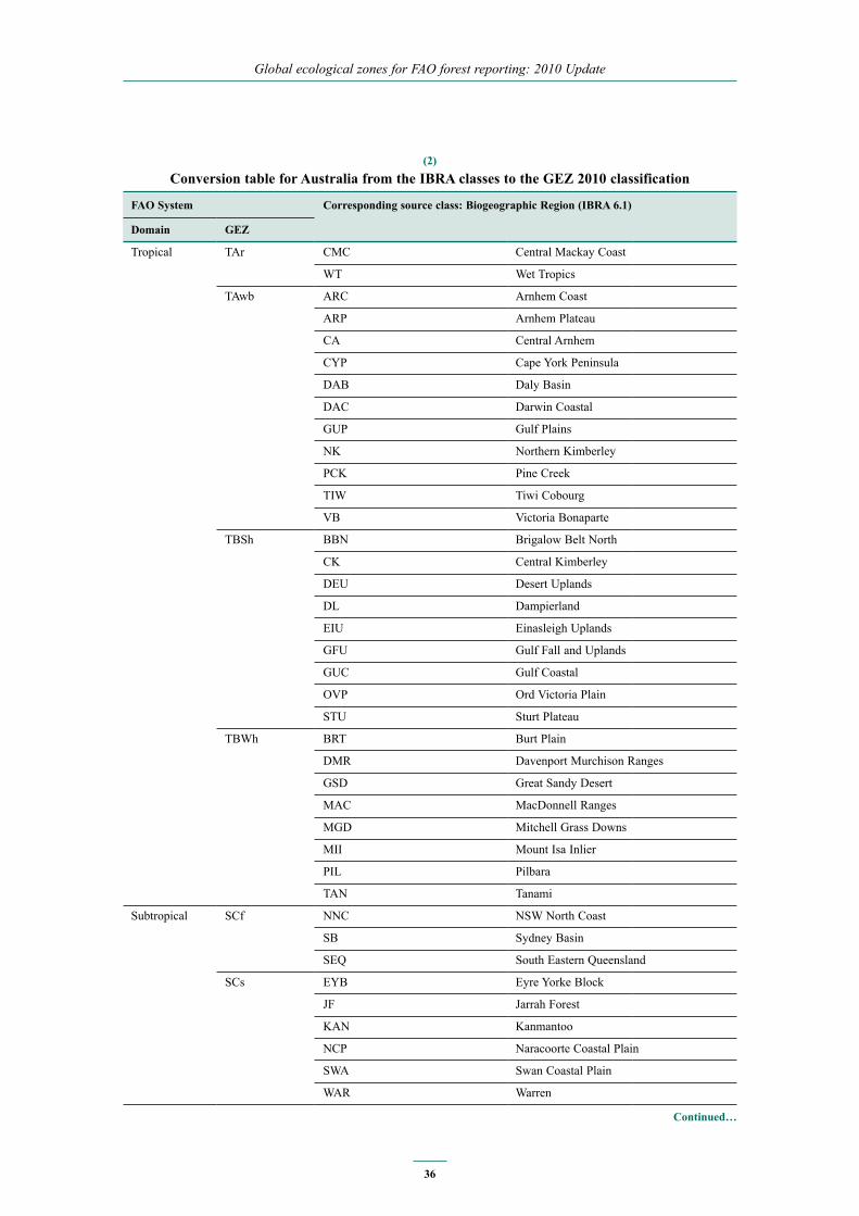
Global ecological zones for fAo forest reporting: 2010 Update
36
(2) conversion table for australia from the IBra classes to the geZ 2010 classification
Fao System corresponding source class: Biogeographic region (IBra 6.1)
domain geZ
Tropical TAr CMC Central Mackay Coast
WT Wet Tropics
TAwb ARC Arnhem Coast
ARP Arnhem Plateau
CA Central Arnhem
CYP Cape York Peninsula
DAB Daly Basin
DAC Darwin Coastal
GUP Gulf Plains
NK Northern Kimberley
PCK Pine Creek
TIW Tiwi Cobourg
VB Victoria Bonaparte
TBSh BBN Brigalow Belt North
CK Central Kimberley
DEU Desert Uplands
DL Dampierland
EIU Einasleigh Uplands
GFU Gulf Fall and Uplands
GUC Gulf Coastal
OVP Ord Victoria Plain
STU Sturt Plateau
TBWh BRT Burt Plain
DMR Davenport Murchison Ranges
GSD Great Sandy Desert
MAC MacDonnell Ranges
MGD Mitchell Grass Downs
MII Mount Isa Inlier
PIL Pilbara
TAN Tanami
Subtropical SCf NNC NSW North Coast
SB Sydney Basin
SEQ South Eastern Queensland
SCs EYB Eyre Yorke Block
JF Jarrah Forest
KAN Kanmantoo
NCP Naracoorte Coastal Plain
SWA Swan Coastal Plain
WAR Warren
continued…

37
Appendix 2
…from previous page
Subtropical SBSh AW Avon Wheatbelt
BBS Brigalow Belt South
CP Cobar Peneplain
DRP Darling Riverine Plains
ESP Esperance Plains
FLB Flinders Lofty Block
GAW Gawler
GS Geraldton Sandplains
MAL Mallee
MDD Murray Darling Depression
NSS NSW South Western Slopes
RIV Riverina
VM Victorian Midlands
SBWh BHC Broken Hill Complex
CAR Carnarvon
CHC Channel Country
COO Coolgardie
CR Central Ranges
FIN Finke
GAS Gascoyne
GD Gibson Desert
GVD Great Victoria Desert
HAM Hampton
LSD Little Sandy Desert
ML Mulga Lands
MUR Murchison
NUL Nullarbor
SSD Simpson Strzelecki Dunefields
STP Stony Plains
YAL Yalgoo
Temperate TeDo BEL Ben Lomond
FLI Flinders
KIN King
SCP South East Coastal Plain
SEC South East Corner
TNM Tasmanian Northern Midlands
TNS Tasmanian Northern Slopes
TSE Tasmanian South East
VVP Victorian Volcanic Plain
TeM AA Australian Alps
NAN Nandewar
NET New England Tablelands
SEH South Eastern Highlands
TCH Tasmanian Central Highlands
TSR Tasmanian Southern Ranges
TWE Tasmanian West
.

Global ecological zones for fAo forest reporting: 2010 Update
38
APPENDIx 3
oceania: Tropical and Subtropical desert description
(Text from Subtropical desert description, Simons, 2001)
Tropical desert (TBWh) and Subtropical desert (SBWh)Deserts occupy a large proportion of Australia, reaching the ocean in the north, south and west. This zone can be separated into the Arid shrublands and the Arid grasslands, which bear similar climates but very different vegetation.
climateThe climate of Australia’s interior shrublands is arid. With no mountains on the west coast the eastward movement of high-pressure systems from the Indian Ocean is not impeded and as a consequence, arid conditions extend from the coast to the interior. The Ecological Zone receives on average less than 250 mm of annual precipitation with a range of between 180 and 350 mm. Fifty percent of this precipitation occurs between December and March. The annual average temperature of the region is 22oC. Average summer maximum temperature is 35oC and average winter maximum is around 23oC. The average minimum temperature in winter is 7oC and in summer the average minimum temperature is 21oC.
The arid grasslands are concentrated within Australia’s largest inland drainage basin leading to Lake Eyre. The region is affected by the same air currents as above, receiving an average annual precipitation of 310 mm. However, monsoonal flooding of several inland river systems has had a major impact on the Physiography of the region which in turn changes the vegetation types that occur. As with all other regions, a precipitation gradient exists, with interior areas receiving 150-200 mm and northern areas receiving up to 400 mm annual precipitation, around 50 percent of which falls between January and March. The annual average temperature across the region is 24oC. Average summer maximum temperature is 36oC and average winter maximum is around 26oC. The average minimum temperature in winter is 8oC and in summer the average minimum temperature is 23oC.
physiographyThe physiography of the arid shrublands is extremely diverse. This ecozone includes: the Great Sandy Desert in the North West; the Tanami Desert in the North; the Gibson and Simpson Deserts in the centre from West to East, the Great Victoria Desert and the Nullabor Plain in the South and the Murchison and Gasgoyne regions in the West, in addition to many other smaller regions with distinct physiography.
The Great Sandy Desert is comprised of Quaternary longitudinal dune fields and gently undulating Jurassic and Cretaceous sandstones. The Tanami Desert is mainly red Quaternary sandplains overlaying Permian and Proterozoic strata which are exposed locally as hills and ranges. The Gibson Desert is comprised of laterised uplands on flat lying Jurassic and Cretaceous sandstones. The Simpson desert is mainly dunefields and sandplains. The Great Victoria Desert is an active sand ridge desert of deep aeolian Quaternary sands. The Nullabor Plain is comprised of Tertiary limestones. The Murchison is mainly Quaternary alluvial and

39
Appendix 3
alluvial surfaces and sandplains surrounding rugged Proteozoic and sedimentary and granite ranges and the Gasgoyne is mainly rugged low Proterozoic sedimentary and granite ranges divided by broad flat valleys.
The arid grasslands are situated in the North East of the Ecological Zone and comprised of two major regions: the Mitchell Grass Downs and Channel Country. The Mitchell Grass Downs are mainly undulating downs on shales and limestones with heavy grey and brown cracking clays. The Channel Country is comprised of mitchell grass downs, braided river systems and low hills on Cretaceous sediments.
VegetationThe enormous local and regional variation in vegetation types across the arid shrubland zone is determined by mean annual rainfall, its seasonal incidence and by soil type. In the “wetter” parts, annual rainfall > 250 mm, Acacia woodlands predominate and mulga (Acacia aneura) is the dominant species over vast tracts of country. The various mulga dominated woodlands show some variation in structure. Mulga itself varies in height from c. 3 – 10 m. The tallest stands are almost closed woodlands with scattered or no shrubs below and a discontinuous grass layer. The woodlands become progressively shorter with diminishing rainfall and in the drier areas they grade into sparse shrublands which, in the driest areas are replaced by hummock grasslands of Triodia, Plectrachne and Zygochloa. Other common Acacia species include A .translucens, A. pachycarpa and A. sowdenii. Casuarina is likewise well represented, occurring both on clays and sands, often in association with a species of Acacia. Eucalyptus is represented by many species, some of which occur in upland, sandy areas also often in combination with Acacia species, whereas other species are restricted to watercourses. In the southern regions on calcareous soils with greater than 250 mm rainfall, many Eucalypts occur in mallee formations (see detailed description above). On soils of finer texture, grasslands or halophytic shrublands occur. Grasslands of the summer rainfall zone are dominated by species of Dichanthium or Astrebla and other less abundant and in the winter rainfall zone by Stipa spp. The halophytic shrublands occupy saline and subsaline soils mainly in drier regions in the south. Other halophytic communities are present on playas.
On the grey and brown clays of the Mitchell Grass Downs and Channel Country, Astrebla spp create almost endless plains of tussock grasses. In recent years the density of these grasslands have been diminished through grazing and the invasion of exotic prickly acacia (Acacia Nilotica) which forms open tree savanna in the northeast of the former treeless plains. The braided river systems are lined with Eucalyptus coolibah woodlands and the low adjacent low hills are often dominated by Chenopodium spp. shrublands.

Global ecological zones for fAo forest reporting: 2010 Update
40
references
Bailey, r.g. (1989) Explanatory supplement to Ecoregions map of the continents. Environmental Conservation, 16, 307-309.
Bailey, r.g. (1994) Ecoregions of the World. USDA Forest Service, Washington DC, USA.Bartholomé, e. & Belward, a.S. (2005) GLC2000: a new approach to global land cover mapping from
Earth observation data. International Journal of Remote Sensing, 26, 1959-1977.Bellan, m.-F. (2000) Ecofloristic Zones and Global Ecological Zoning of Africa, South America and
Tropical Asia. FAO, Rome, Unpublished Report.Bohn, u., gollub, g., & hettwer, c. (2000) Karte der natürlichen Vegetation Europas. Massstab
1:2.500.000 Karten und Legende. Bundesamt für Naturschutz, Bonn, Germany.Bow, J., Josse, c., Sayre, r., Sotomayor, L., & Touval, J. (2008) Terrestrial Ecosystems of South
America. The Nature Conservancy and Natureserve, Arlington, VA.cec (1997) Ecological Regions of North America. Commission for Environmental Cooperation,
Montreal, Canada.crawford, r.m.m. (2008) Plants at the Margin: ecological limits and climate change. Cambridge
University Press, Cambridge.di gregorio, a., ed. (2005) Land Cover Classification System (LCCS) Version 2. Classification concepts
and user manual. http://www.fao.org/docrep/008/y7220e/y7220e00.htm. FAO, Rome.drigo, r. (2005) Trends and patterns of tropical land use change. In: Bonell, M. and L.A. Bruijnzeel
(Eds.). Forests, Water and People in the Humid Tropics. Cambridge University Press. Cambridge. pp 9-39.
eTc Biodiversity (2006) Indicative map of European biogeographical regions. Methodology and development. Muséum National d’Histoire Naturelle, Paris.
ewel, J.J. & Whitmore, J.L. (1973) The ecological life zones of Puerto Rico and U.S. Virgin Islands. USDA Forest Servise, INstitute of Tropical Forestry, Research Paper ITF-018.
Fao (1989) Classification and mapping of vegetation types in tropical Asia. FAO, Rome.Fao (1993) Forest Resources Assessment 1990. Tropical countries. FAO Forestry Paper 112. FAO,
Rome.Fao (2001) Global Forest Resources Assessment 2000. Main Report. FAO Forestry Paper 140. FAO,
Rome.Fao (2010) Global Forest Resources Assessment 2010. Main Report. FAO Forestry Paper 163. FAO,
Rome.Fao, Jrc, & SdSu (2009) The 2010 Global Forest Resources Assessment Remote Sensing Survey: an
outline of the objectives data, methods and approach. FRA Working Paper 155. FAO with FRA RSS partners, Rome.
Fao naFc (2010) Inventory and Monitoring Group minutes, May 2010. Guadalajara, Mexico. Accessed on 4 August 2011. http://www.fs.fed.us/global/nafc/inventory/activities.htm.
Fischer, g., van Velthuizen, h., Shah, m., & nachtergaele, F. (2002) Global Agro-ecological Assessment for Agriculture in the 21st Century: Methodology and Results. Research Report RR-02-02. IIASA and FAO, Rome.
gonzalez, p., nielson, r., Lenihan, J.m., & drapek, r.J. (2010) Global patterns in vulnerability of ecosystems to vegetation shifts due to climate change. Global Ecology and Biogeography, 19, 755--768.
grubb, p.J. (1971) Interpreting the “Massenserhebung” effect on tropical mountains. Nature, 229, 44-45.helmer, e.h., ramos, o., Lopez, T.d.m., Quinonones, m., & diaz, W. (2002) Mapping forest type
and land cover of Puerto Rico, a component of the Caribbean Biodiversity Hotspot. Caribbean Journal of Science, 38, 165-183.

41
References
hiederer, r., ramos, F., capitani, c., koeble, r., Blujdea, V., mulligan, d., & marelli, L. (2010) Biofuels: a new methodology to estimate GHG emissions from global land use change. European Commission JRC, Ispra.
hutchinson, m.F., mcIntyre, S., hobbs, r.J., Stein, J.L., garnett, S., & kinloch, J. (2005) Integrating a global agro-climatic classification with bioregional boundaries in Australia. Global Ecology and Biogeography, 14, 197-212.
Ipcc (2006). Forest Land. In 2006 IPCC Guidelines for National Greenhouse Gas Inventories. Vol. 4. Agriculture, forestry and other Land Use. Ch. 4. (ed IPCC). IGES Hayama, Japan.
Iremonger, S. & cross, h. (2000) FRA 2000 Global Ecological Zones mapping. Workshop report. Cambridge, 28-30 July 1999. FRA Working Paper 26. FAO, Rome.
Isachenko, T.I., karamysheva, Z.V., Ladygina, g.m., & Safronova, I.n. (1990) Map of vegetation of the USSR. Scale: 1:4Million. Institute for Geography, RAS., Moscow.
köppen, W. (1931) Grundriss der Klimakunde. Walter de Grwyter, Berlin.Lavenu, F., Bellan, m.-F., & meste, c. (1988) Carte ecofloristique de l’Amerique du Sud. FAO, Rome.Lunetta, r.L., knoght, F.k., ediriwickrema, J., Lyon, J.g., & Worthy, L.d. (2006) Land cover
change detection using multi-temporal MODIS NDVI data. Remote Sensing of Environment., 105, 142-154.
metzger, m.J., Bunce, r.g.h., Jongman, r.h.g., mucher, c.a., & Watkins, J.W. (2005) A climatic stratification of the environment of Europe. Global Ecology and Biogeography., 14, 549-563.
metzger, m.J., Bunce, r.g.h., Jongman, r.h.g., Sayre, r., Trabucco, a., & Zomer, r. (in review) A high resolution bioclimate map of the world: a unifying framework for global biodiversity research. Global Ecology and Biogeography.
muchoney, d.m.m., Iremonger, S., & Wright, r. (1994) Rapid Ecological Assessment. Blue and John Crow Mountains National Park, Jamaica. The Nature Conservancy., Arlington, USA.
norfalise, a. (1987) Map of the Natural Vegetation of the member countries of the European Community and of the Council of Europe. Office for Official Publications of the European Communities, Luxembourg.
preto, g. (1998) A proposal for the preparation of the Global Eco-floristic map for FRA2000 FAO, Rome, Unpublished Report.
Sayre, r., comer, p., Warner, h., & cress, J. (2009) A New Map of Standardized Terrestrial Ecosystems of the Conterminous United States. Professional Paper 1768. U.S. Geological Survey.
Schepaschenko, d., mccallum, I., Shvidenko, a., Fritz, S., kraxner, F., & obersteiner, m. (2010) A new hybrid land cover dataset for Russia: a methodology for integrating statistics, remote sensing and in situ information. Journal of Land Use Science. Available on-line Dec 2010., 1-15.
Sharma, m.k. (1986) Ecofloristic zone and vegetation maps of tropical continental Asia. FAO, Rome.
Sharma, m.k. (1988) Eco-floristic zone map of Africa. FAO, Rome.Simons, h. (2001) FRA 2000. Global Ecological Zoning for the Global Forest Resources Assessment
2000. FRA Working Paper 56. FAO, Rome.Simons, h., Singh, k.d., Zhu, Z., & davis, r. (1999) FRA 2000. A concept and strategy for
Ecological Zoning for the Global Forest Resources Assessment 2000. Interim Report. FRA Working Paper 20. FAO, Rome.
Singh, k.d. (2000). The global/regional ecological zone classification concept and definition. In fRA 2000 Global Ecological Zone mapping. Workshop Report. Cambridge, 28-30 July 1999. fRA Working Paper 26, pp 9-10. FAO, Rome.
Tateishi, r., uriyangqai, B., al-Bilbisi, h., ghar, m.a., Tsend-ayush, J., kobayashi, T., kasimu, a., hoan, n.T., Shalaby, a., alsaaideh, B., enkhzaya, T., gegentana, & Sato, h.p. (2011) Production of global land cover data - GLCNMO. International Journal of Digital Earth, 4, 22-49.
Thackway, r. & cresswell, I.d. (1995) An Interim Biogeographic Regionalisation for Australia: a framework for setting priorities in the National Reserves system cooperative program. Version 4.0. Canberra, Australian Nature Conservation Agency.

Global ecological zones for fAo forest reporting: 2010 Update
42
Tnc (2009) Terrestrial Ecoregional Boundaries Shapefile. The Nature Conservancy, Arlington, USA.Trewartha, g.T. (1968) An Introduction to Climate., 4th edn. McGraw-Hill, New York.uneSco & Fao (1969) Vegetation map of the Mediterranean zone. UNESCO and FAO.Walter, h. (1973) Vegetation of the Earth in relation to Climate and Eco-physical Conditions.
Springer-Verlag, New York.WWF (2000) Terrestrial Ecoregions of the World. WWF.Zheng, d.Z. (1992) Geographic distribution of China’s main forests. Nanjing Forestry.Zhu, Z. (1997) Develop a new Global Ecological Zone map for Global FRA2000. FAO, Rome,
Unpublished Report.

FRA 2015
Terms and Definitons
december, 2012
Forest resources Assessment Working Paper 180