gis-pro 2013: urisa's
TRANSCRIPT


September 16-19, 2013www.urisa.org
M a r k y o u r C a l e n d a r !
Join us in Providence, Rhode Island for
GIS-Pro 2013: URISA’s 51st Annual Conference for GIS Professionals
URISA's 51st Annual Conference for GIS ProfessionalsGIS-Pro 2013
need new colors

Volume 25 • No. 1 • 2013
Journal of the Urban and Regional Information Systems Association
Contents
5 Relating GIS&T and Project Management Bodies of Knowledge to Projects Perceived as Successes
Patrick J. Kennelly
19 Perspectives on the Evaluation of Geo-ICT for Sustainable Urban Governance: Implications for E-government Policy
Diego D. Navarra
29 Building a Highway Linear Referencing System from Preexisting Reference Marker Measurements for Transportation Data Management
John M. Bigham and Sanghyeok Kang
39 Sociopolitical Contexts and Geospatial Data—the Case of Dane County
Falguni Mukherjee
47 An Operational Approach for Building Extraction from Aerial Imagery
Liora Sahar and Nickolas Faust
Papers of Practice, Technical Reports and Industry Notes
53 Deployment of a National Geocoding Service: Cuban Experience
Carlos José de Armas García and Andrei Abel Cruz Gutiérrez
63 Evaluating Neighborhoods through Empirical Analysis and Geographic Information Systems
Greg Rybarczyk and Rama Prasada Mohapatra

2 URISA Journal • Vol. 25, No. 1 • 2013
Publisher: Urban and Regional Information Systems Association
Editor-in-Chief: Dr. Piyushimita (Vonu) Thakuriah
Journal Coordinator: Wendy Nelson
Electronic Journal: http://www.urisa.org/urisajournal
Journal
EDITORIAL OFFICE: Urban and Regional Information Systems Association, 701 Lee Street, Suite 680, Des Plaines, Illinois 60016; Voice (847) 824-6300; Fax (847) 824-6363; E-mail [email protected].
SUBMISSIONS: This publication accepts from authors an exclusive right of first publication to their article plus an accompanying grant of non-exclusive full rights. The publisher requires that full credit for first publication in the URISA Journal is provided in any subsequent electronic or print publications. For more information, the “Manuscript Submission Guidelines for Refereed Articles” is available on our website, www.urisa.org, or by calling (847) 824-6300.
SUBSCRIPTION AND ADVERTISING: All correspondence about advertising, subscriptions, and URISA memberships should be directed to: Urban and Regional Information Systems Association, 701 Lee Street, Suite 680, Des Plaines, Illinois 60016; Voice (847) 824-6300; Fax (847) 824-6363; E-mail [email protected].
URISA Journal is published two times a year by the Urban and Regional Information Systems Association.
© 2013 by the Urban and Regional Information Systems Association. Authorization to photocopy items for internal or personal use, or the internal or personal use of specific clients, is granted by permission of the Urban and Regional Information Systems Association.
Educational programs planned and presented by URISA provide attendees with relevant and rewarding continuing education experience. However, neither the content (whether written or oral) of any course, seminar, or other presentation, nor the use of a specific product in conjunction there-with, nor the exhibition of any materials by any party coincident with the educational event, should be construed as indicating endorsement or approval of the views presented, the products used, or the materials exhibited by URISA, or by its committees, Special Interest Groups, Chapters, or other commissions.
SUBSCRIPTION RATE: One year: $295 business, libraries, government agencies, and public institutions. Individuals interested in subscriptions should contact URISA for membership information.
US ISSN 1045-8077

URISA Journal • Vol. 25, No. 1 • 2013 3
URISA Journal Editor
Editor-in-Chief
Dr. Piyushimita (Vonu) Thakuriah, Department of Urban Studies and School of Engineering, University of Glasgow, United Kingdom
Thematic Editors:
Sustainability Analysis and Decision Support Systems: Timothy Nyerges, University of Washington
Participatory GIS and Related Applications: Laxmi Ramasubramanian, Hunter College
Social, Economic, Governance and Political Sciences: Francis Harvey, University of Minnesota
GIScience: Harvey Miller, University of Utah
Urban and Regional Systems and Modeling: Itzhak Benenson, Tel Aviv University
Editorial Board
Jochen Albrecht, Hunter College
Peggy Agouris, Center for Earth Observing and Space Research, George Mason University, Virginia
David Arctur, Open Geospatial Consortium
Michael Batty, Centre for Advanced Spatial Analysis, University College London (United Kingdom)
Kate Beard, Department of Spatial Information Science and Engineering, University of Maine
Yvan Bédard, Centre for Research in Geomatics, Laval University (Canada)
Itzhak Benenson, Department of Geography, Tel Aviv University (Israel)
Al Butler, GISP, Milepost Zero
Barbara P. Buttenf ield , Department of Geography, University of Colorado
Keith C. Clarke, Department of Geography, University of California-Santa Barbara
David Coleman, Department of Geodesy and Geomatics Engineering, University of New Brunswick (Canada)
Paul Cote, Graduate School of Design, Harvard University
David J. Cowen, Department of Geography, University of South Carolina
William J. Craig, GISP, Center for Urban and Regional Affairs, University of Minnesota
Robert G. Cromley, Department of Geography, University of Connecticut
Michael Gould, Environmental Systems Research Institute
Klaus Greve, Department of Geography, University of Bonn (Germany)
Daniel A. Griffith, Geographic Information Sciences, University of Texas at Dallas
Francis J. Harvey, Department of Geography, University of Minnesota
Bin Jiang, University of Gävle, Sweden
Richard Klosterman, Department of Geography and Planning, University of Akron
Jeremy Mennis, Department of Geography and Urban Studies, Temple University
Nancy von Meyer, GISP, Fairview Industries
Harvey J. Miller, Department of Geography, University of Utah
Zorica Nedovic-Budic, School of Geography, Planning and Environmental Policy, University College, Dublin (Ireland)
Timothy Nyerges, University of Washington, Department of Geography, Seattle
Harlan Onsrud, Spatial Information Science and Engineering, University of Maine
Zhong-Ren Peng, Department of Urban and Regional Planning, University of Florida
Laxmi Ramasubramanian, Hunter College, Department of Urban Affairs and Planning, New York City
Carl Reed, Open Geospatial Consortium
Claus Rinner, Department of Geography, Ryerson University (Canada)
Monika Sester, Institute of Cartography and Geoinformatics, Leibniz Universität Hannover, Germany
David Tulloch, Department of Landscape Architecture, Rutgers University
Stephen J . Ventu ra , Depar t ment o f Environmental Studies and Soil Science, University of Wisconsin-Madison
Barry Wellar, Department of Geography, University of Ottawa (Canada)
Lyna Wiggins, Department of Planning, Rutgers University
F. Benjamin Zhan, Department of Geography, Texas State University-San Marcos
Editorial Board


URISA Journal • Kennelly 5
IntroductIonThe most common metric used to assess effective project manage-ment is project success or project failure. Certain measures are used for determining failure rates in the oft-cited Chaos Reports of 1995 and 2004 (The Standish Group). Using data collected from surveys, interviews, and focus groups, projects were assigned to three categories based on measures of cost and time overruns, as well as assessments of content deficiencies (The Standish Group 1995). According to the 2004 Chaos Report, 18 percent of proj-ects failed, 53 percent were challenged, and 29 percent succeeded.
These studies have merit for providing straightforward evaluations of project success when detailed data on cost, timing, and scope—the so-called triple constraint of project manage-ment—are available. Their focus on project performance in a small number of managerial knowledge areas, however, may oversimplify planning approaches to achieve project success. For example, issues of cost may have arisen because of poor com-munication practices, which might be remedied in future projects at no additional cost.
When projects include requirements in specific technical areas such as geospatial technology, consideration of project suc-cess must encompass both general project management issues as well as domain specific issues. One way to conduct an analysis of successful geotechnical projects would be to consider all areas of knowledge related to geospatial technology and project manage-ment simultaneously. Such analysis is facilitated by geospatial technology and general project management both having refer-ence frameworks, the geographic information science and technol-ogy (GIS&T) and project management (PM) bodies of knowledge (BoK), respectively.
Although these frameworks are well established as a series of knowledge areas, extensive datasets of geospatial projects are not readily available, and procedures for mapping project components to the BoKs are not well established. This study looks at 101 reports on predominantly geospatial projects writ-ten by geospatial industry professionals. Their reports discussed geospatial projects, focused on geospatial and managerial issues that arose, and included their opinions on whether the projects were successful. This study uses these reports to map geospatial components of the projects to the GIS&T BoK knowledge areas, and management issues to PM knowledge areas. This study also offers the author’s perception, based on observations in the report and the author’s opinion, on each project as successful or failure-prone. The procedure for mapping geospatial components to the GIS&T BoK, managerial issues to the PM BoK, and criteria for judging projects perceived as successful and failure-prone are discussed in the methodology.
Within these frameworks, the overall objective of this study is to determine how the perceived success of geospatial projects is related to both project management issues and geospatial knowledge. The specific objectives of this study are to determine: 1. How frequently projects perceived as failure-prone are
associated with geotechnical issues;2. If projects that integrate more numerous GIS&T knowledge
areas are more often perceived as failure-prone;3. If projects that experience problems in a greater number of
PM knowledge areas are more often perceived as failure-prone;
4. If projects experiencing problems in any pair-wise combinations of PM functions (summary categories of PM
relating GIS&t and Project Management Bodies of Knowledge to Projects Perceived as Successes
Patrick J. Kennelly
Abstract: This study examines 101 geospatial projects and the perception of participating geospatial professionals on their suc-cess. It organizes their discussion of technical aspects of the work and managerial problems that arose within the frameworks of the geographic information science and technology (GIS&T) and the project management (PM) bodies of knowledge (BoK), respectively. Based on this author’s appraisal of projects perceived as failure-prone (those perceived as failures, containing significant pitfalls, or of uncertain outcome by the professionals), technical issues are rarely cited as the cause of failure-prone projects, and integration of more numerous GIS&T BoK knowledge areas are associated with a smaller percentage of failure-prone projects. Results also reveal that most failure-prone projects have serious management issues in more than one nonfacilitating knowledge area of the PM BoK, a trend that could be useful in tracking at the onset of a project at risk of being failure-prone. Finally, by mapping managerial problems within PM BoK knowledge areas to GIS&T knowledge areas, this study identifies problems in particular managerial areas for projects with particular GIS&T components. Such competency-based approaches will allow geospatial project managers and professionals to better plan projects and recognize common pitfalls.
6 URISA Journal • Vol. 25, No. 1 • 2013
knowledge areas) are more often perceived as failure-prone; and
5. What types of project management problems might be expected with projects utilizing various GIS&T knowledge areas, and which of these cross-discipline combinations are most often associated with projects perceived as failure-prone.
This analysis extensively utilizes the GIS&T and PM BoKs, two examples of professional fields that recognize the importance of com-prehensively inventorying areas of knowledge. BoKs also have been documented in other disciplines, including civil engineering (The Body of Knowledge Committee 2008), software engineering (Abran et al. 2001), software quality measurement (Schneidewind 2002), enterprise architecture (Hagan 2004), configuration management (The Configuration Management Community 2009), and business analysis (Brennan 2000). In addition to serving as inventories of skills and knowledge, these BoKs can be used for endeavors important to the health and development of a profession or organization, includ-ing certification, accreditation, strategic planning, and curriculum assessment or development (Prager and Plewe 2009). Following is a brief overview of the GIS&T and PM BoKs.
GIS&t BoKThe GIS&T BoK (DiBiase et al. 2007) is organized in a strongly hierarchical fashion. At the highest level are the ten knowledge areas listed with two-letter abbreviations that follow:• Analytical Methods (AM)• Conceptual Foundations (CF)• Cartography and Visualization (CV)• Design Aspects (DA)• Data Modeling (DM)• Data Manipulation (DN)• Geocomputation (GC)• Geospatial Data (GD)• GIS&T and Society (GS)• Organizational and Institutional Aspects (OI)
At the level beneath are a total of 73 units, with the number of units per knowledge area varying from three to 12. In this study, components of projects were mapped to the unit level. The level beneath units includes the most detailed topics, with the number of topics per unit varying from two to nine.
PM BoKThe PM BoK does not have so detailed a hierarchy, but it does organize knowledge areas at a higher level into three categories called functions (Project Management Institute 2004). These func-tions are core, facilitating, and integrative. The latter consists of only one knowledge area (project integration management) that integrates managerial components from all other PM knowledge areas. The functions and their underlying knowledge areas* are
listed as follows:• Core functions
• Time• Scope• Cost• Quality
• Facilitating functions• Human resources• Communication• Risk• Procurement
• Integrative functions• Project integration
Beneath the knowledge area level, there is no more detailed structural breakdown. Instead, these knowledge areas are dis-cussed in terms of specific tools, techniques, methodologies, and best practices that may be utilized to ensure project success (Project Management Institute 2004, Schwalbe 2009). Many project management studies focus on how to best avoid issues in one or more knowledge area, such as quality (Futrell et al. 2001, Crosby 1979) or risk (Raz and Michael 2001, Wideman 1992).
MethodoloGyThe methodology for analyzing project reports involved the fol-lowing four components. First, geospatial reports were collected over a span of three years. Second, each project was categorized as either being perceived as successful or failure-prone. Third, components of each project were mapped to units of the GIS&T BoK. Finally, issues identified in each project were mapped to knowledge areas in the PM or GIS&T BoK, depending on whether the nature of the issue was managerial or geotechnical.
GeoSPatIal Project rePortSThe data for this study are 101 project reports, varying in length from three pages to five pages. The authors of these reports generally were full-time workers in geospatial technology and part-time graduate students beginning a geospatial technology project management class in a professional Master’s of GIS de-gree program. These reports were collected and evaluated by this author, while serving as the course instructor, over a period of nine terms during three years.
Reports were designed to allow students to reflect on their perception of a project in which they participated, before a more formal survey of the field of geospatial project management. Specific instructions for writing a portion of this report are given as follows:
Document a project, preferably a geospatial project from your organization. In documenting the project, include informa-tion that you perceive as important to understanding how the project progressed from a geotechnical and managerial perspective. You may include information on cost, timing, scope, quality, or other aspects you think were key. You also
* This study preceded “Project Stakeholder Management” being added as a tenth knowledge area in the PM BOK Guide, 5th Edition (2012).

URISA Journal • Kennelly 7
should make a determination of whether the project was a success or a failure. You should describe the project in your own words, but indicate the source of your information.
PercePtIon of Project SucceSSThis author/class instructor, taking the opinions and supporting evidence of the students into account, made a determination of projects he perceived as probable successes. It is important to stress that the author has no additional information other than that supplied by the students, so in nearly all cases a traditional declaration of project success was difficult or impossible to make. Instead, this author categorized all projects into two nominal classes. The first class consists of projects perceived as failure-prone, which includes those projects that students perceived as being failures, with significant pitfalls and uncertain outcomes. Projects with significant pitfalls, although sometimes deemed successful by students, generally had such severe issues that their scope or qual-ity seemed seriously compromised. Projects of uncertain success generally were so poorly scoped that the student and/or instruc-tor could not evaluate whether the project objectives were met.
The second class consists of projects perceived as successful. It includes all 78 projects perceived by students as successful. Twenty of these projects included metrics that, if reported properly by students, indicate success in terms of meeting project objectives on schedule and budget. The remaining 58, although lacking such evidence, did not include any elements such as cost over-runs, missed deadlines, or failure to meet project objectives that would explicitly indicate failure. The two pending projects are not included in the analysis.
Project coMPonentS and the GIS&t BoKThis author/instructor examined geospatial project reports and identified all components of projects that corresponded to a GIS&T unit and were utilized to meet the project’s geotechnical needs. Geospatial projects may use specialized knowledge from a combination of any or all knowledge areas, or might require expertise from only one specific topic of one particular unit of a single knowledge area. For example, a project to develop a “custom tool to map attributes of residential meters” involved a design aspect (DA) to design the tool, a data manipulation (DN) component to put attributes in the proper format, and a GIS&T and Society (GS) component to provide information to the customers.
In their reports, students were not required to discuss how components of their projects fit into the GIS&T BoK. Instead, this author/instructor reviewed all reports and mapped student discussion to the BoK. Students described technical components of projects in sufficient detail for the author/instructor to identify specific “units” of GIS&T knowledge areas utilized, with units often but not always occurring in different knowledge areas. Any
uncertainty of mapping to specific units should be mitigated by analysis for this study being conducted at the higher knowledge area level.
relatInG ISSueS to the PM BoKMost project reports included discussions of some issues or problems that arose during the projects. Some were geospatial technology issues, but the vast majority were managerial issues. Based on the report’s description of the issue, this author nomi-nally mapped each issue to one of the PM knowledge areas. In some cases, such as a project’s duration taking much longer than proposed, the choice of knowledge area (Time) was straightfor-ward, given the information provided. When possible, the author attempted to look at causality and be as consistent as possible with the information provided. For example, a team lacking some of the geotechnical skills necessary to complete a project may face issues of meeting deadlines (Time), staying on budget (Cost), or meeting requirements (Scope). The author, however, mapped this issue to the “Human Resources” PM knowledge area, as an appropriately skilled team member or technical training could eliminate this issue.
data coMPIlatIon and dISPlayData on perceived success, PM knowledge areas in which issues arose, and GIS&T knowledge areas to which project components correspond were collected in a summary table and used to create the graphs in the Results section. The summary table also allowed for creation of a display unique to this study and referred to as a knowledge matrix.
A knowledge matrix considers pair-wise combinations of knowledge areas from the two BoKs, mapping problems in PM knowledge areas to all the GIS&T knowledge areas that these projects contain. These cross-pairings do not consider whether a particular PM issue arose because of efforts in one GIS&T knowledge area or another in the project, and in most cases such causality was impossible to determine. Thus, a project utilizing three GIS&T knowledge areas and having problems arise in three PM knowledge areas would be mapped to nine separate cross-pairings represented by grid cells in the knowledge matrix.
Given ten GIS&T knowledge areas that could represent components of geospatial projects and nine PM knowledge areas were potential problems could arise, a maximum of 90 grid cells is possible between the two BoKs. In this study, projects included technical components from only eight of the GIS&T knowledge areas (none from Geocomputation (GC) or Conceptual Founda-tions (CF)). Additionally, some GIS&T knowledge areas were never associated with problems in particular PM knowledge areas. As a result, this study mapped 262 cross-pairings to a total of 59 grid cells in the matrix.
8 URISA Journal • Vol. 25, No. 1 • 2013
ResultsA table summarizing the analysis and listing report names, edited to ensure anonymity, is included in the Appendix. This table was constructed to address all the objectives outlined in the intro-duction of this study. Each row represents a project. The table includes three columns to account for the maximum number of managerial problems reported (PM1 to PM3), and five columns for the maximum number of GIS&T components integrated into a project (GIST1 to GIST5). This format allows projects to be categorized and evaluated on perceived success, the number or category of PM knowledge areas in which issues were discussed, and the number or category of GIS&T knowledge areas included as components in the project.
Of the 101 reports, 78 percent were perceived to be success-ful, 20 percent were perceived to be failure-prone, and 2 percent were pending. This degree of perceived project failure is similar to failures found in the CHAOS Report (2004), which averaged 18 percent of projects studied. Of the 20 failure-prone projects, 13 included serious issues with cost, time, or scope. Such issues often are interrelated and known to make project success unattainable. Of the remaining seven, four had critical issues with communica-tion among partners, clients, or workers and management. The other three had issues with integration that in two cases arose from personnel turnover or reassignment.
Technical IssuesOne result of this study is that the reports are much more likely to discuss project management issues rather than geotechnical issues. While 80 percent of the reports discussed at least one management issue, only 9 percent reported technical issues worthy of discussion. Of those reporting technical issues, however, six of nine were associated with projects perceived as failure-prone. The common thread among most of these technical failures was that the project was a first or early attempt to use a particular technology within the organization.
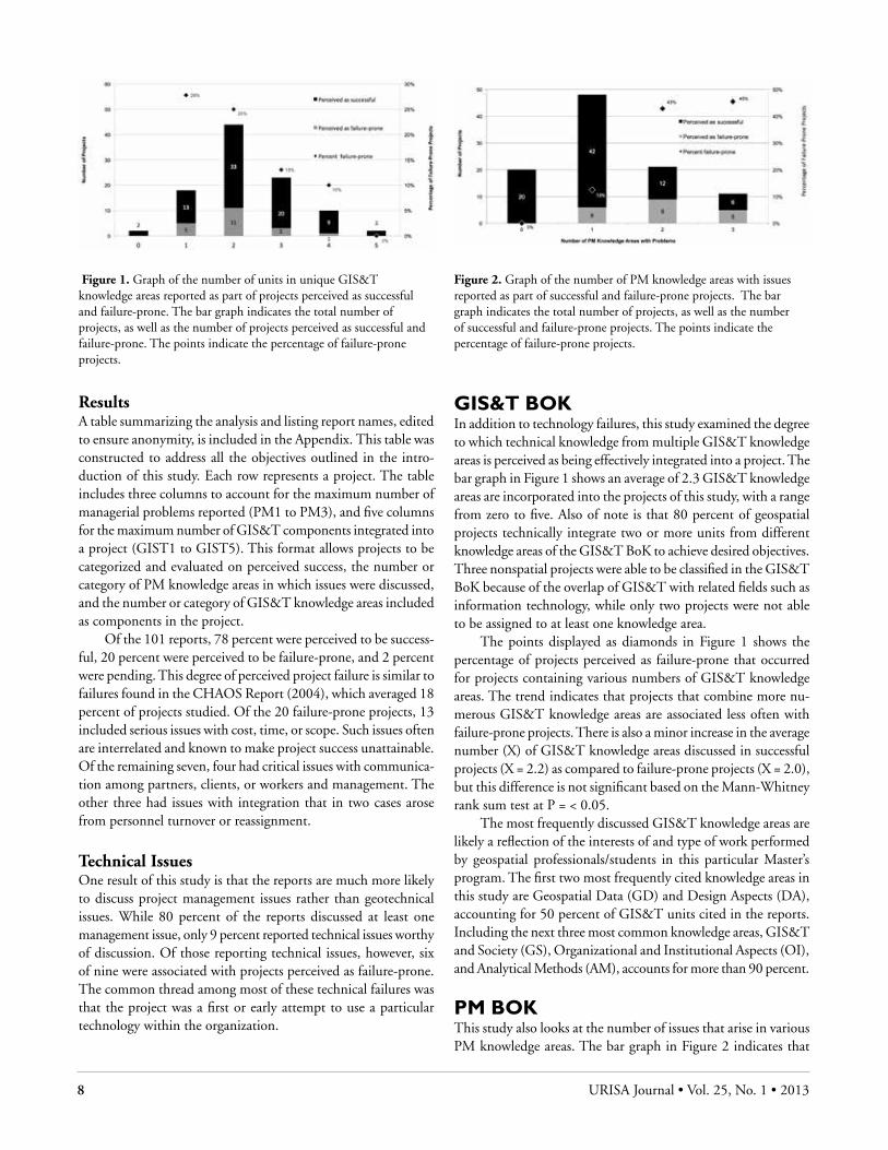
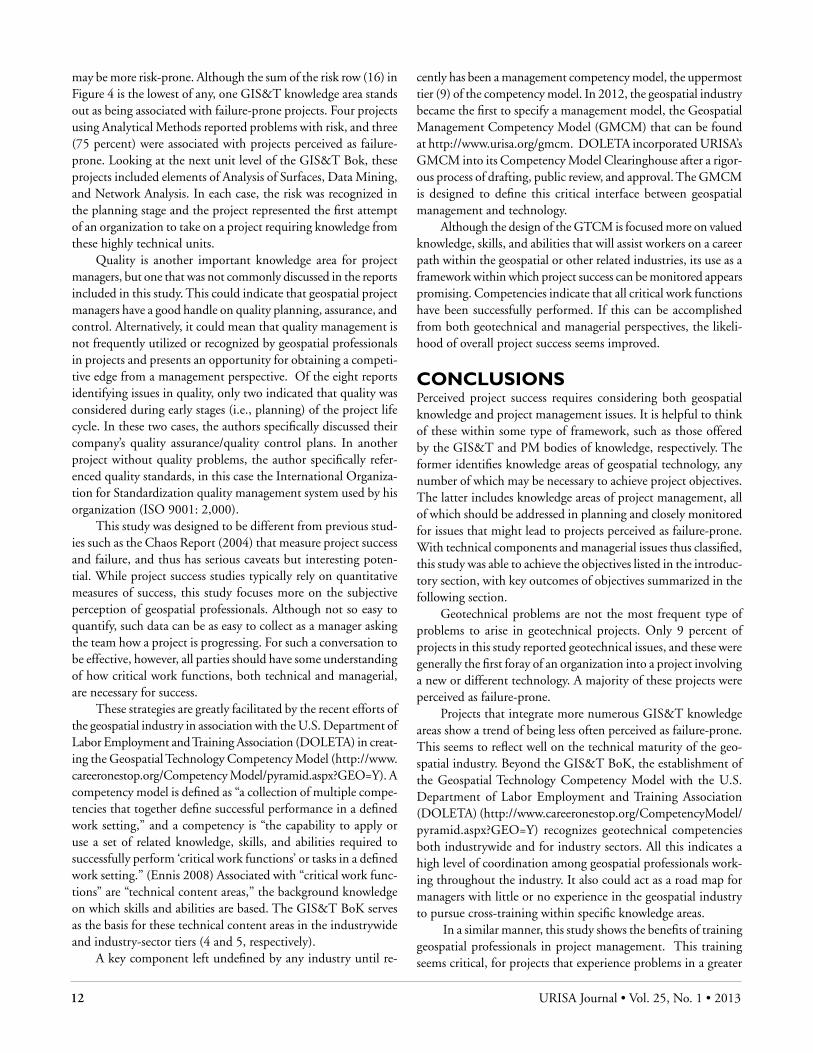
GIS&t BoKIn addition to technology failures, this study examined the degree to which technical knowledge from multiple GIS&T knowledge areas is perceived as being effectively integrated into a project. The bar graph in Figure 1 shows an average of 2.3 GIS&T knowledge areas are incorporated into the projects of this study, with a range from zero to five. Also of note is that 80 percent of geospatial projects technically integrate two or more units from different knowledge areas of the GIS&T BoK to achieve desired objectives. Three nonspatial projects were able to be classified in the GIS&T BoK because of the overlap of GIS&T with related fields such as information technology, while only two projects were not able to be assigned to at least one knowledge area.
The points displayed as diamonds in Figure 1 shows the percentage of projects perceived as failure-prone that occurred for projects containing various numbers of GIS&T knowledge areas. The trend indicates that projects that combine more nu-merous GIS&T knowledge areas are associated less often with failure-prone projects. There is also a minor increase in the average number (X) of GIS&T knowledge areas discussed in successful projects (X = 2.2) as compared to failure-prone projects (X = 2.0), but this difference is not significant based on the Mann-Whitney rank sum test at P = < 0.05.
The most frequently discussed GIS&T knowledge areas are likely a reflection of the interests of and type of work performed by geospatial professionals/students in this particular Master’s program. The first two most frequently cited knowledge areas in this study are Geospatial Data (GD) and Design Aspects (DA), accounting for 50 percent of GIS&T units cited in the reports. Including the next three most common knowledge areas, GIS&T and Society (GS), Organizational and Institutional Aspects (OI), and Analytical Methods (AM), accounts for more than 90 percent.
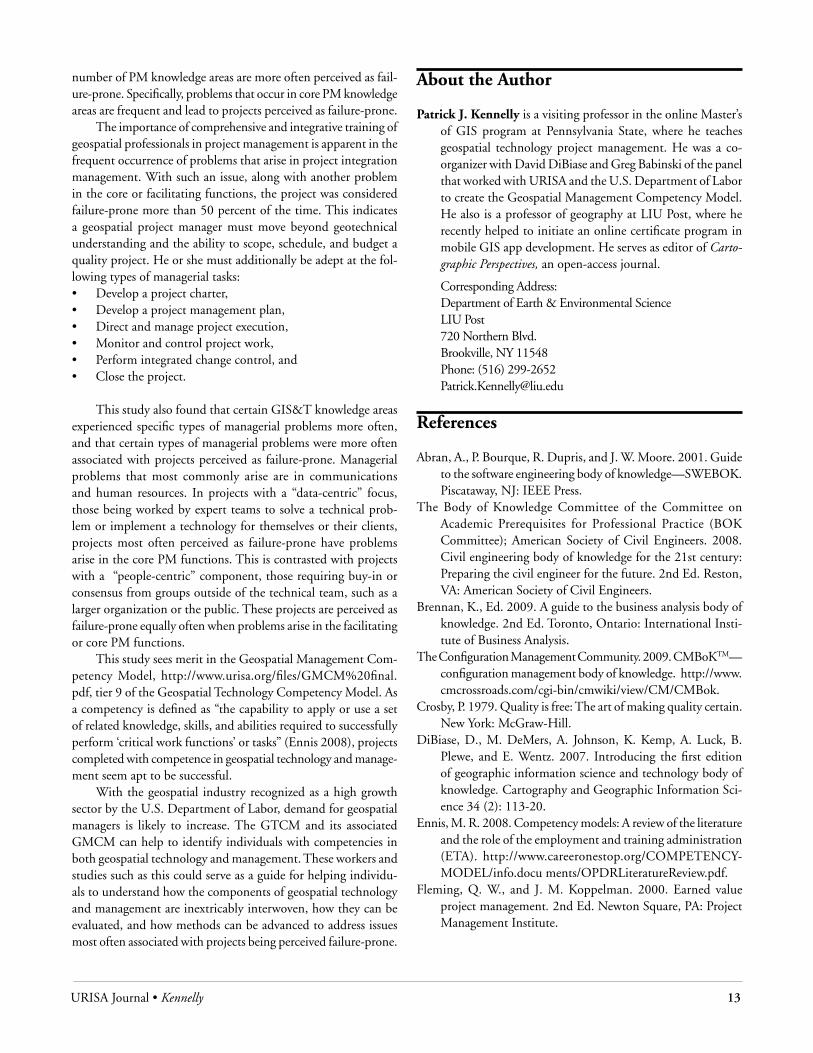
PM BoKThis study also looks at the number of issues that arise in various PM knowledge areas. The bar graph in Figure 2 indicates that
Figure 1. Graph of the number of units in unique GIS&T knowledge areas reported as part of projects perceived as successful and failure-prone. The bar graph indicates the total number of projects, as well as the number of projects perceived as successful and failure-prone. The points indicate the percentage of failure-prone projects.
Figure 2. Graph of the number of PM knowledge areas with issues reported as part of successful and failure-prone projects. The bar graph indicates the total number of projects, as well as the number of successful and failure-prone projects. The points indicate the percentage of failure-prone projects.

URISA Journal • Kennelly 9
problems occurred in an average of 1.2 PM knowledge areas per project, with a range from zero (no problems discussed regard-ing a successful project) to three (three different issues related to three unique project management knowledge areas). The points in Figure 2 do not follow a linear trend, but show that projects reporting issues in more than one PM knowledge areas are more often perceived as failure-prone, as might be expected. This also is apparent in the large disparity between the average number (X) of knowledge areas experiencing problems discussed in reports on successful projects (X = 1.1) and reports on failure-prone projects (X = 2.0). This is a significant difference based on the Mann-Whitney rank sum test at P = < 0.001.
A problem in only one PM BoK knowledge area does not often lead to failure, but these occurrences are worth noting. Of the six failure-prone projects with one management problem, four proved to be communication issues. Specifically, failure to establish or utilize key communication channels among cowork-ers, managers, clients, etc., in the planning and implementation phases of the project life cycle often resulted in projects perceived as failure-prone. This can be compared with a dozen projects perceived as successful that experienced some communication problem. In all of these cases, the proper channels of communica-tion were properly established, but unclear communication led to less severe problems.
In most cases, projects perceived as failure-prone had issues in more than one knowledge area of the PM BoK (Figure 2). To investigate, this study evaluated pair-wise combinations of PM knowledge areas when more that one problem occurred in more than one area. These are generalized to the function level of the PM BoK to provide a more general summary of results.
Figure 3 shows the project management “functions” associ-ated with pair-wise combinations of issues in PM knowledge areas for projects perceived as successful and failure-prone. The bar graph shows the number and breakdown of projects perceived as successful and failure-prone. The points show the percentage
of projects perceived as failure-prone. The detrimental nature of issues that arise in core or integrative knowledge areas is appar-ent. Any issue in a core or integrative knowledge area occurring in conjunction with a problem in any other knowledge area results in a perceived failure-prone rate of at least 50 percent. This contrasts sharply with projects that have problems within Facilitating-Facilitating functions. None of these projects were considered failure-prone.
Cross-Discipline Knowledge MatricesEach problem that arises in a specific PM knowledge area can be associated with at least one specific GIS&T knowledge area for the projects in this study. By looking at these cross-discipline pair-wise relationships and mapping results to a knowledge matrix, it is possible to see the type of managerial problems most likely to arise for projects that contain geotechnical components in particular GIS&T knowledge areas. Generalizing the PM knowledge areas to the function level aggregates greater numbers of problems into fewer categories. It also indicates whether projects utilizing particular GIS&T knowledge areas are more often perceived as failure-prone if issues arise in core versus facilitating PM functions.
The top row of Figure 4 shows the type of GIS&T knowledge areas utilized in the projects that reported no managerial problems. Summing this row, there were 39 geospatial components discussed in these 20 problem-free projects.
The remainder of Figure 4 represents a knowledge matrix with problems that arose in particular PM knowledge areas mapped to all GIS&T knowledge areas utilized in projects per-ceived as both successful and failure-prone. Numbers indicate the total number of problems discussed for each combination. At this granular level of inquiry, where more than one-third (31 of 72) of the cells contain zero, one, or two problems, and only six cells have values of ten or more, the percentage of problems associated with projects perceived as successful versus failure-prone is not shown.
The rows are PM knowledge areas and are grouped by the core, integrative, and facilitating functions from top to bottom. The columns are the GIS&T knowledge areas and are ordered by the sum of each column in the matrix proper. Moving from left to right, these sums vary from 65 to 5. This wide disparity of problems is more associated with how many projects reported on particular GIS&T knowledge areas being utilized (and the career interests of the geospatial professionals writing the reports), and should not be taken as an indication that projects that incorporate certain knowledge areas are more or less likely to be problem-free. Nevertheless, variations in values found in columns of the matrix reveal where problems are most and least likely to arise.
Focusing on the PK knowledge areas in which problems occur most frequently, the facilitating knowledge areas of com-munication and human resources always rank first and second for the four most discussed GIS&T knowledge areas (the four left columns of Figure 4). Project managers utilizing these GIS&T knowledge areas should expect such problems outside of any discussion of perceived project failure and success.
Figure 3. Pareto chart of pair-wise combinations of PM functions with perceived problems in successful and failure-prone projects. The bar graph indicates the total number of projects, as well as the number of projects perceived as successful and failure-prone. The points display the percentage of failure-prone projects.

10 URISA Journal • Vol. 25, No. 1 • 2013
Table 1 summarizes the data in Figure 4 to the function level of the PM BoK in its rows entitled Total. Because the integra-tive function includes one knowledge area (Integration), while core and facilitating functions each contain four, the former was omitted from Table 1. The subsequent rows report on how many problems in each grouping were associated with projects perceived as failure-prone, and the final rows report percentage of projects failure-prone.
dIScuSSIonThis study is not designed to assign causes of failure to projects perceived as failure-prone. It does, however, reveal trends in the type of GIS&T project components and the problems that arise in PM knowledge areas that are most frequently associated with projects perceived as failure-prone by geospatial professionals. Project managers can use these results to help plan geospatial projects or to track important project metrics once the project is initiated.
Project managers are served well by understanding geo-spatial technology and its integration. Most project reports in this study (91 percent) do not include a discussion of techno-logical problems. Also, projects that incorporate more GIS&T knowledge areas are less often considered failure-prone (Figure 1). Both of these observations reflect well on the technical maturity of the geospatial industry and its workforce and their abilities to integrate disparate GIS&T knowledge areas from a technology standpoint.
Exploring the reasons that projects that incorporate more numerous GIS&T bodies of knowledge have lower failure rates is beyond the scope of this study, but it may simply be a reflection of the necessary geotechnical complexity of achieving desirable project objectives. It also may be the result of projects with a geospatial technology focus requiring more experienced geospatial professionals. A detailed look at the dozen projects utilizing four or five GIS&T knowledge areas indicates that contributions from
Table 1. Comparisons of problems in core and facilitating PM functions for projects with a component from each of the eight GIS&T knowledge areas discussed in this study
GeospatialData
DesignAspects
GIS&T &Society
O & I Aspects
AnalyticalMethods
DataModeling
DataManip.
Cartog. &Vis.
TotalCore 21 23 15 13 11 11 3 3Facilitating 39 33 22 19 13 4 2 1
Perceived Failure-ProneCore 6 11 5 2 4 8 2 0Facilitating 6 7 7 3 4 1 2 0
Percentage Perceived Failure-ProneCore 29% 48% 33% 15% 36% 73% 67% 0%Facilitating 15% 21% 32% 16% 31% 25% 100% 0%
Figure 4. A knowledge matrix showing pair-wise connections between PM and GIS&T knowledge areas. Total GIS&T knowledge areas associated with PM problems decreases from left to right. The two most common PM knowledge areas for problems to arise in the first four columns are communications and human resources management.

URISA Journal • Kennelly 11
all GIS&T knowledge areas cited seem essential to achieving the desired objectives.
A geospatial manager should expect managerial problems to arise, as 80 percent of the projects in this study reported some such problems. If the first problem to arise is a communication problem, it is essential that the manager ensure that all proper channels of communication have been well established. For example, a “kickoff meeting” that includes all important team members and stakeholders makes these channels of communica-tion apparent and personal, and can help to avoid this potential problem (Kerzner 2007).
If a geospatial project has more than one managerial issue, it is important for the project manager to recognize the PM functions in which these problems occur. If one of the problems is in a core function, this study would indicate that the project has only about a 50 percent chance of being perceived as successful (Figure 2). One important observation difficult to extract from this study is the level of severity of the problems, especially in the core func-tions. This author observed, however, that in some reports, steps were taken early to mitigate the effect of issues with scope, timing, cost, or quality, tending to make projects more often perceived as successful. Such early recognition underscores the importance of project management tracking tools such as earned value manage-ment (Fleming and Koppelman 2000, 2002) to recognize and correct such problems at an early stage in the project.
Although issues in core functions are critical in projects with more than one problem, project managers cannot afford to ignore the importance of integration management. Integration manage-ment is defined as coordinating all other PK knowledge areas throughout the project’s life cycle. It includes six main processes: developing the project charter, developing the project management plan, directing and managing project execution, monitoring and controlling project work, performing integrated change control, and closing the project (PMBOK Guide 2009). For geospatial professionals taking on new project management roles, some of these processes may be less familiar or require more specialized knowledge than do the core functions of scoping a project, track-ing a budget, or staying on schedule. Effective mastery of these integrative processes may require training in project management or guidance from more experienced project managers.
Although all these integrative processes are well defined from the project management perspective, what is less well defined is how a geospatial manager can bring his or her knowledge of the technol-ogy to bear on these critical processes, such as when developing the project management plan. Although a work breakdown structure (WBS) associated with these plans can be created with readily ac-cessible software and a somewhat formulaic approach of breaking down objectives to summary tasks and then to smaller tasks (Project Management Institute 2006), it would be difficult or impossible for a geospatial project manager to create such a WBS without a work-ing understanding of all the technical requirements of such projects.
Communication and human resources issues seem espe-cially prevalent facilitating problems. For communication issues, problems with communication channels never being established
often lead to projects perceived as failure-prone, but frequent is-sues associated with miscommunications are not uncommon in projects perceived as successful. In human resources management, changes in personnel often are associated with projects perceived as failure-prone, while issues associated with training, time off, or team conflicts often are more minor issues that frequently occur in projects perceived as successful.
Further trends are revealed in the cross-discipline knowledge matrix of Figure 4 and its summary in Table 1. The two most frequently cited GIS&T knowledge areas, Geospatial Data (GD) and Design Aspects (DA), are approximately twice as likely to be considered failure-prone from problems arising in the core versus facilitating knowledge areas, even though more problems are reported in the facilitating areas. Such projects reported in this study tended to be “technocentric”; they focused on the technol-ogy, were worked by a team familiar with geospatial technology, and had fairly limited requirements for interpersonal interactions outside of the team. Facilitating issues, especially in communica-tion and human resources, will continue to arise, but seem more easily resolved by the teams in this study’s projects, which often were interacting collaboratively on a daily basis.
These results can be compared to the next two most fre-quently cited GIS&T knowledge areas, GIS&T and Society (GS) and Organizational and Institutional Aspects (OI). Projects that include such components are just as likely to be perceived failure-prone from issues that arise in facilitating or core PM knowledge areas. These projects tended to more “people-centric,” focused on the ways in which organizations, partners, or the public ei-ther accesses or interacts with geospatial technology. Some steps that could have mitigated problems in projects from this study include identifying champions or sponsors, communicating with important stakeholders, and a more thorough understanding or appreciation of the organizational culture (Keen 1981).
Fewer examples of problems were reported for other GIS&T knowledge area columns in Figure 4, making subsequent percent-ages in Table 1 more difficult to interpret. One number worth noting, however, was that for projects with a Data Modeling component that experienced problems in the core PM functions, 73 percent (8 of 11) were perceived as failure-prone. Such projects were generally “technocentric,” and often represented a first foray of an organization into a project requiring knowledge from highly technical units of this knowledge area.
To be able to utilize the knowledge matrix presented as Figure 4 to report on projects perceived as successful or failure-prone at the knowledge area level would require GIS&T projects utilizing a greater variety of knowledge areas and a much greater number of examples. With such data, each cell could show the percentage of projects perceived as failure-prone. Although cur-rently some cells are associated with just a few projects, they still provide some glimpse into concerns with specific combinations of GIS&T knowledge area project components and PM knowl-edge area issues.
For example, project managers must understand the risk associated with a project, and certain GIS&T knowledge areas
12 URISA Journal • Vol. 25, No. 1 • 2013
may be more risk-prone. Although the sum of the risk row (16) in Figure 4 is the lowest of any, one GIS&T knowledge area stands out as being associated with failure-prone projects. Four projects using Analytical Methods reported problems with risk, and three (75 percent) were associated with projects perceived as failure-prone. Looking at the next unit level of the GIS&T Bok, these projects included elements of Analysis of Surfaces, Data Mining, and Network Analysis. In each case, the risk was recognized in the planning stage and the project represented the first attempt of an organization to take on a project requiring knowledge from these highly technical units.
Quality is another important knowledge area for project managers, but one that was not commonly discussed in the reports included in this study. This could indicate that geospatial project managers have a good handle on quality planning, assurance, and control. Alternatively, it could mean that quality management is not frequently utilized or recognized by geospatial professionals in projects and presents an opportunity for obtaining a competi-tive edge from a management perspective. Of the eight reports identifying issues in quality, only two indicated that quality was considered during early stages (i.e., planning) of the project life cycle. In these two cases, the authors specifically discussed their company’s quality assurance/quality control plans. In another project without quality problems, the author specifically refer-enced quality standards, in this case the International Organiza-tion for Standardization quality management system used by his organization (ISO 9001: 2,000).
This study was designed to be different from previous stud-ies such as the Chaos Report (2004) that measure project success and failure, and thus has serious caveats but interesting poten-tial. While project success studies typically rely on quantitative measures of success, this study focuses more on the subjective perception of geospatial professionals. Although not so easy to quantify, such data can be as easy to collect as a manager asking the team how a project is progressing. For such a conversation to be effective, however, all parties should have some understanding of how critical work functions, both technical and managerial, are necessary for success.
These strategies are greatly facilitated by the recent efforts of the geospatial industry in association with the U.S. Department of Labor Employment and Training Association (DOLETA) in creat-ing the Geospatial Technology Competency Model (http://www.careeronestop.org/Competency Model/pyramid.aspx?GEO=Y). A competency model is defined as “a collection of multiple compe-tencies that together define successful performance in a defined work setting,” and a competency is “the capability to apply or use a set of related knowledge, skills, and abilities required to successfully perform ‘critical work functions’ or tasks in a defined work setting.” (Ennis 2008) Associated with “critical work func-tions” are “technical content areas,” the background knowledge on which skills and abilities are based. The GIS&T BoK serves as the basis for these technical content areas in the industrywide and industry-sector tiers (4 and 5, respectively).
A key component left undefined by any industry until re-
cently has been a management competency model, the uppermost tier (9) of the competency model. In 2012, the geospatial industry became the first to specify a management model, the Geospatial Management Competency Model (GMCM) that can be found at http://www.urisa.org/gmcm. DOLETA incorporated URISA’s GMCM into its Competency Model Clearinghouse after a rigor-ous process of drafting, public review, and approval. The GMCM is designed to define this critical interface between geospatial management and technology.
Although the design of the GTCM is focused more on valued knowledge, skills, and abilities that will assist workers on a career path within the geospatial or other related industries, its use as a framework within which project success can be monitored appears promising. Competencies indicate that all critical work functions have been successfully performed. If this can be accomplished from both geotechnical and managerial perspectives, the likeli-hood of overall project success seems improved.
concluSIonSPerceived project success requires considering both geospatial knowledge and project management issues. It is helpful to think of these within some type of framework, such as those offered by the GIS&T and PM bodies of knowledge, respectively. The former identifies knowledge areas of geospatial technology, any number of which may be necessary to achieve project objectives. The latter includes knowledge areas of project management, all of which should be addressed in planning and closely monitored for issues that might lead to projects perceived as failure-prone. With technical components and managerial issues thus classified, this study was able to achieve the objectives listed in the introduc-tory section, with key outcomes of objectives summarized in the following section.
Geotechnical problems are not the most frequent type of problems to arise in geotechnical projects. Only 9 percent of projects in this study reported geotechnical issues, and these were generally the first foray of an organization into a project involving a new or different technology. A majority of these projects were perceived as failure-prone.
Projects that integrate more numerous GIS&T knowledge areas show a trend of being less often perceived as failure-prone. This seems to reflect well on the technical maturity of the geo-spatial industry. Beyond the GIS&T BoK, the establishment of the Geospatial Technology Competency Model with the U.S. Department of Labor Employment and Training Association (DOLETA) (http://www.careeronestop.org/CompetencyModel/pyramid.aspx?GEO=Y) recognizes geotechnical competencies both industrywide and for industry sectors. All this indicates a high level of coordination among geospatial professionals work-ing throughout the industry. It also could act as a road map for managers with little or no experience in the geospatial industry to pursue cross-training within specific knowledge areas.
In a similar manner, this study shows the benefits of training geospatial professionals in project management. This training seems critical, for projects that experience problems in a greater
URISA Journal • Kennelly 13
number of PM knowledge areas are more often perceived as fail-ure-prone. Specifically, problems that occur in core PM knowledge areas are frequent and lead to projects perceived as failure-prone.
The importance of comprehensive and integrative training of geospatial professionals in project management is apparent in the frequent occurrence of problems that arise in project integration management. With such an issue, along with another problem in the core or facilitating functions, the project was considered failure-prone more than 50 percent of the time. This indicates a geospatial project manager must move beyond geotechnical understanding and the ability to scope, schedule, and budget a quality project. He or she must additionally be adept at the fol-lowing types of managerial tasks:• Develop a project charter,• Develop a project management plan,• Direct and manage project execution,• Monitor and control project work,• Perform integrated change control, and• Close the project.
This study also found that certain GIS&T knowledge areas experienced specific types of managerial problems more often, and that certain types of managerial problems were more often associated with projects perceived as failure-prone. Managerial problems that most commonly arise are in communications and human resources. In projects with a “data-centric” focus, those being worked by expert teams to solve a technical prob-lem or implement a technology for themselves or their clients, projects most often perceived as failure-prone have problems arise in the core PM functions. This is contrasted with projects with a “people-centric” component, those requiring buy-in or consensus from groups outside of the technical team, such as a larger organization or the public. These projects are perceived as failure-prone equally often when problems arise in the facilitating or core PM functions.
This study sees merit in the Geospatial Management Com-petency Model, http://www.urisa.org/files/GMCM%20final.pdf, tier 9 of the Geospatial Technology Competency Model. As a competency is defined as “the capability to apply or use a set of related knowledge, skills, and abilities required to successfully perform ‘critical work functions’ or tasks” (Ennis 2008), projects completed with competence in geospatial technology and manage-ment seem apt to be successful.
With the geospatial industry recognized as a high growth sector by the U.S. Department of Labor, demand for geospatial managers is likely to increase. The GTCM and its associated GMCM can help to identify individuals with competencies in both geospatial technology and management. These workers and studies such as this could serve as a guide for helping individu-als to understand how the components of geospatial technology and management are inextricably interwoven, how they can be evaluated, and how methods can be advanced to address issues most often associated with projects being perceived failure-prone.
About the Author
Patrick J. Kennelly is a visiting professor in the online Master’s of GIS program at Pennsylvania State, where he teaches geospatial technology project management. He was a co-organizer with David DiBiase and Greg Babinski of the panel that worked with URISA and the U.S. Department of Labor to create the Geospatial Management Competency Model. He also is a professor of geography at LIU Post, where he recently helped to initiate an online certificate program in mobile GIS app development. He serves as editor of Carto-graphic Perspectives, an open-access journal.
Corresponding Address: Department of Earth & Environmental Science LIU Post 720 Northern Blvd. Brookville, NY 11548 Phone: (516) 299-2652 [email protected]
References
Abran, A., P. Bourque, R. Dupris, and J. W. Moore. 2001. Guide to the software engineering body of knowledge—SWEBOK. Piscataway, NJ: IEEE Press.
The Body of Knowledge Committee of the Committee on Academic Prerequisites for Professional Practice (BOK Committee); American Society of Civil Engineers. 2008. Civil engineering body of knowledge for the 21st century: Preparing the civil engineer for the future. 2nd Ed. Reston, VA: American Society of Civil Engineers.
Brennan, K., Ed. 2009. A guide to the business analysis body of knowledge. 2nd Ed. Toronto, Ontario: International Insti-tute of Business Analysis.
The Configuration Management Community. 2009. CMBoKTM—configuration management body of knowledge. http://www.cmcrossroads.com/cgi-bin/cmwiki/view/CM/CMBok.
Crosby, P. 1979. Quality is free: The art of making quality certain. New York: McGraw-Hill.
DiBiase, D., M. DeMers, A. Johnson, K. Kemp, A. Luck, B. Plewe, and E. Wentz. 2007. Introducing the first edition of geographic information science and technology body of knowledge. Cartography and Geographic Information Sci-ence 34 (2): 113-20.
Ennis, M. R. 2008. Competency models: A review of the literature and the role of the employment and training administration (ETA). http://www.careeronestop.org/COMPETENCY-MODEL/info.docu ments/OPDRLiteratureReview.pdf.
Fleming, Q. W., and J. M. Koppelman. 2000. Earned value project management. 2nd Ed. Newton Square, PA: Project Management Institute.

14 URISA Journal • Vol. 25, No. 1 • 2013
Fleming, Q. W., and J. M. Koppelman. 2002. Using earned value management. Cost Engineering 44 (9): 32-38.
Futrell, R. T., L. I. Schafer, and D. F. Shafer. 2001. Quality software project management. Upper Saddle River, NJ: Prentice Hall PTR.
Geospatial Technology Competency Model. 2012. CareerOne-Stop. U.S. Department of Labor, Employment and Training Administration. http://www.careeronestop.org/Competen-cyModel/pyramid. aspx?GEO=Y, March 17, 2012.
Hagan, P. J. 2004. Guide to the (evolving) enterprise architecture body of knowledge. McLean, VA: The Mitre Corporation.
Keen, P. 1981. Information systems and organizational change. Communications of the ACM 24 (1): 24-33.
Kerzner, H. 2009. Project management: A systems approach to planning, scheduling and controlling. Hoboken, NJ: John Wiley and Sons, Inc.
Prager, S., and B. Plewe. 2009. Assessment and evaluation of GI-Science curriculum using the geographic information science and technology body of knowledge. Journal of Geography in Higher Education 33 (Supplement 1): S46-S69.
Project Management Institute. 2004. A guide to the project management body of knowledge. 3rd Ed. Newtown Square, PA: Project Management Institute.
Project Management Institute. 2006. Practice standard for work breakdown structures. 2nd Ed. Newtown Square, PA: Project Management Institute.
Raz, T., and E. Michael. 2001. Use and benefits of tools for project risk management. International Journal of Project Management 19 (1): 9-17.
Schneidewind, N. E. 2002. Body of knowledge for software qual-ity measurement. Computer 35 (2): 77-83.
Schwalbe, K. 2009. Information technology project management. 6th Ed. Boston, MA: Thomson Course Technology.
The Standish Group. 1995. CHAOS report. www.standishgroup.com.
The Standish Group. 2004. Latest Standish Group CHAOS report shows project success rates have improved by 50%. www.standishgroup.com.
Wideman, R. M. 1992. Project and program risk management: A guide to managing project risks and opportunities. Upper Darby, PA: Project Management Institute.
Appendix
List of geospatial projects, their perceived success, the project management body of knowledge (PM BoK) knowledge areas in which problems arose (PM1–PM3), and the geographic informa-tion science and technology body of knowledge (GIS&T BoK) knowledge areas with which the technical components of projects were associated (GIST1–GIST5).
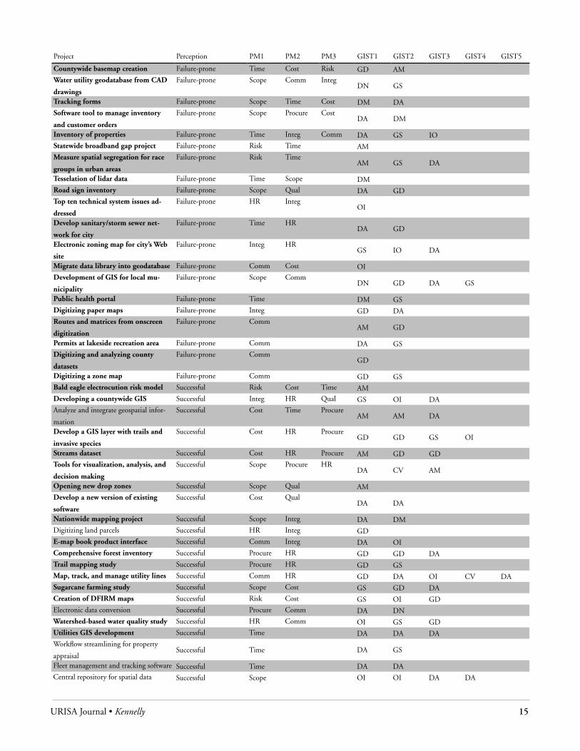
URISA Journal • Kennelly 15
Project Perception PM1 PM2 PM3 GIST1 GIST2 GIST3 GIST4 GIST5
Countywide basemap creation Failure-prone Time Cost Risk GD AMWater utility geodatabase from CAD
drawings
Failure-prone Scope Comm IntegDN GS
Tracking forms Failure-prone Scope Time Cost DM DASoftware tool to manage inventory
and customer orders
Failure-prone Scope Procure CostDA DM
Inventory of properties Failure-prone Time Integ Comm DA GS IOStatewide broadband gap project Failure-prone Risk Time AMMeasure spatial segregation for race
groups in urban areas
Failure-prone Risk TimeAM GS DA
Tesselation of lidar data Failure-prone Time Scope DMRoad sign inventory Failure-prone Scope Qual DA GDTop ten technical system issues ad-
dressed
Failure-prone HR IntegOI
Develop sanitary/storm sewer net-
work for city
Failure-prone Time HRDA GD
Electronic zoning map for city’s Web
site
Failure-prone Integ HRGS IO DA
Migrate data library into geodatabase Failure-prone Comm Cost OIDevelopment of GIS for local mu-
nicipality
Failure-prone Scope CommDN GD DA GS
Public health portal Failure-prone Time DM GSDigitizing paper maps Failure-prone Integ GD DARoutes and matrices from onscreen
digitization
Failure-prone CommAM GD
Permits at lakeside recreation area Failure-prone Comm DA GSDigitizing and analyzing county
datasets
Failure-prone CommGD
Digitizing a zone map Failure-prone Comm GD GSBald eagle electrocution risk model Successful Risk Cost Time AMDeveloping a countywide GIS Successful Integ HR Qual GS OI DAAnalyze and integrate geospatial infor-
mation
Successful Cost Time ProcureAM AM DA
Develop a GIS layer with trails and
invasive species
Successful Cost HR ProcureGD GD GS OI
Streams dataset Successful Cost HR Procure AM GD GDTools for visualization, analysis, and
decision making
Successful Scope Procure HRDA CV AM
Opening new drop zones Successful Scope Qual AMDevelop a new version of existing
software
Successful Cost QualDA DA
Nationwide mapping project Successful Scope Integ DA DMDigitizing land parcels Successful HR Integ GDE-map book product interface Successful Comm Integ DA OIComprehensive forest inventory Successful Procure HR GD GD DATrail mapping study Successful Procure HR GD GSMap, track, and manage utility lines Successful Comm HR GD DA OI CV DASugarcane farming study Successful Scope Cost GS GD DACreation of DFIRM maps Successful Risk Cost GS OI GDElectronic data conversion Successful Procure Comm DA DNWatershed-based water quality study Successful HR Comm OI GS GDUtilities GIS development Successful Time DA DA DAWorkflow streamlining for property
appraisalSuccessful Time DA GS
Fleet management and tracking software Successful Time DA DACentral repository for spatial data Successful Scope OI OI DA DA
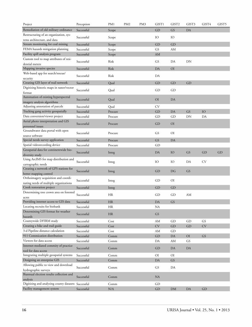
16 URISA Journal • Vol. 25, No. 1 • 2013
Project Perception PM1 PM2 PM3 GIST1 GIST2 GIST3 GIST4 GIST5
Remediation of old military ordinance Successful Scope GD GS DARestructuring of an organization, sys-
tems architecture, and dataSuccessful Scope IO IO
Stream monitoring for coal mining Successful Scope GD GDFEMA hazards mitigation planning Successful Scope GS AMFacility spill analysis program Successful Scope AMCustom tool to map attributes of resi-
dential metersSuccessful Risk GS DA DN
Mapping invasive species Successful Risk DA OIWeb-based app for search/rescue/
securitySuccessful Risk DA
Creating GIS layer of trail network Successful Qual GD GD GDDigitizing historic maps in raster/vector
formatSuccessful Qual GD GD
Automation of existing hyperspectral
imagery analysis algorithmsSuccessful Qual OI DA
Adjusting annotation of parcels Successful Qual CVTracking gang activity geospatially Successful Procure GD DA GS IOData conversion/viewer project Successful Procure GD GD DN DAAerial photo interpretation and GIS
personnel issuesSuccessful Procure GD OI
Groundwater data portal with open
source softwareSuccessful Procure GS OI
Special needs survey application Successful Procure GS DASpatial videorecording device Successful Procure GDGeospatial data for continentwide bio-
diversity studySuccessful Integ DA IO GS GD GD
Using ArcIMS for map distribution and
cartographic needsSuccessful Integ IO IO DA CV
Creating a network of GPS stations for
better mapping controlSuccessful Integ GD DG GS
Orthoimagery acquisition and coordi-
nating needs of multiple organizationsSuccessful Integ GD OI
Creek restoration project Successful Integ GD GDDetermining tree crown area on forested
acresSuccessful HR GD GD AM
Providing internet access to GIS data Successful HR DA GSLocating recruits for biobank Successful HR NADetermining GIS format for weather
hazardsSuccessful HR GS
Countywide DFIRM study Successful Cost AM GD GD GSCreating a bike and trail guide Successful Cost CV GD GD CV3-d Pipeline distance calculation Successful Cost AM GD911 Commication distribution Successful Comm GD DA OI GSViewers for data access Successful Comm DA AM GSInternet-mediated commity of practice
tool for data accessSuccessful Comm GD DA DA
Integrating multiple geospatial systems Successful Comm OI OIDesigning an enterprise GIS Successful Comm DA GSAllowing public to view and download
hydrographic surveysSuccessful Comm GS DA
Biannual election results collection and
analysisSuccessful Comm NA
Digitizing and analyzing county datasets Successful Comm GDFacility management system Successful N/A GD DM DA GD

URISA Journal • Kennelly 17
Project Perception PM1 PM2 PM3 GIST1 GIST2 GIST3 GIST4 GIST5
Security for Olympics games Successful N/A GD GD OICreating a base map from aerial imagery Successful N/A GD GD DNStandardizing data storage for multiple
projectsSuccessful N/A GD OI DA
Personnel deployment Successful N/A IO DA CVPreliminary integrated geologic map
databaseSuccessful N/A GS OI
Converting to a GIS-based tropical
cyclone daily warning systemSuccessful N/A DA GS
Finding unexploded ordinances Successful N/A GD GDDeveloping GIS data and creating print
mapsSuccessful N/A GD GD
Acquiring true color orthoimagery Successful N/A GD GDNational realignment to build balanced
sales territoriesSuccessful N/A OI DA
Migrating pipeline data into geodata-
baseSuccessful N/A DA DA
Natural gas resource mapping Successful N/A GS DAViewshed modeling Successful N/A AM AMLocating satellite offices based on work-
load dataSuccessful N/A OI AM
Metadata creation Successful N/A GDDeriving features with imagery analysis Successful N/A GDEverglades restoration study Successful N/A DMEfficient follow-up testing based on
routingSuccessful N/A AM
Creating photorealistic buildings for
visualizationPending HR Procure Cost DM CV DA
Identifying desirable land tracts for
acquisitionPending N/A AM

URISA Journal • Navarra 19
IntroductIonGeographic information and communication technologies (Geo-ICT) are the end result of the combination of geographic informa-tion (including spatial, geologic, geodetic, geometric, etc.) and Information and Communication Technology (ICT). Geo-ICT includes geographic information systems (GIS), land information systems (LIS), spatial decision support systems (SDSS), spatial data infrastructures (SDI), and spatial information infrastructures (SII). These typically are implemented for their contribution to the efficiency and effectiveness of the organization of government, to improve public sector governance, to increase the availability and accessibility of government’s services, as well as to improve general planning, coordination, and cooperation (Akingbade, Navarra, and Georgiadou 2009).
Geo-ICT thus are becoming an integral part of the study of the evolution of e-government policy initiatives for urban governance across the developed and the developing world to connect government agencies and institutions, to promote the reorganization of government’s internal and external informa-tion flows, activities, and functions in order to shift government’s service delivery over the Internet (Ciborra and Navarra 2005). E-government also is expected to benefit the community by drawing together the public sector, civil society, and interna-tional actors, as well as by improving consultation with, and participation by, all spheres of society, and to achieve more participatory processes of governance and decision making (Navarra and Cornford 2007).
Urban governance concerns the rules, processes, and struc-tures through which decisions are made about access to urban land and the use of its resources. It is an important element of the many complex challenges the world faces today, including adaptation and mitigation to climate change, rapid urbanization, growing food and energy insecurity, increased natural disasters, etc. (Palmer, Fricskas, and Wehrmann 2009). Nevertheless, no common understanding exists about the way in which the progress
and future direction of these projects and initiatives should be evaluated for sustainable urban governance.
Therefore, what disciplines and approaches help us to un-derstand the value of Geo-ICT for sustainable urban governance? What are the implications for public sector governance and for e-government policy? The following section outlines the research approach. The next section reviews the interdisciplinary literature on the value of Geo-ICT. Finally, policy implications on the value of Geo-ICT for e-government policy and for public sector gover-nance are outlined. Conclusions about the evaluation of Geo-ICT in e-government for sustainable urban governance follow.
reSearch aPProach The paper’s research approach is both interdisciplinary and deductive to empirical (Bailey 1994). We started with the conceptualization of the characteristics and dimensions of new interdisciplinary perspectives to be able to provide an overview of the key ideas of the existing literature. We reviewed classified case studies, findings from previous evaluation studies of Geo-ICT in different countries, and exemplary Geo-ICT practices in order to understand Geo-ICT and their value for public sector governance. This approach allowed us to be able to conceptualize new characteristics and dimensions of Geo-ICT emerging from academic literature and studies made both in developed as well as in developing countries.
For instance, a recent European Umbrella Organization for Geographic Information (EUROGI) report suggests that virtually in every European country, e-government and Geo-ICT initia-tives are proceeding along separate tracks in almost complete isolation from each other (EUROGI 2008). Yet the evolution of e-government initiatives is an important determinant of the value of geoinformation (Longhorn and Blakemore 2008: 12). In the European region, for instance, “Spatial Data Infrastructure is an important part of the e-government initiative of the Bavarian government” (Stoessel 2006); and in countries outside of Europe,
Perspectives on the evaluation of Geo-Ict for Sustainable urban Governance: Implications for e-government Policy
Diego D. Navarra
Abstract: This paper introduces three interdisciplinary perspectives applicable to the evaluation of geographic information and communication technologies (Geo-ICT) for sustainable urban governance. The first perspective sees Geo-ICT as a public good that can be used to understand the spatial structure of the urban economy by optimizing the spatial distribution of natural, economic, and social activities. The second perspective sees Geo-ICT primarily as a standardizable, quantitative, and formal way to mediate geoinformation with the aim to make space controllable, measurable, and quantifiable. Finally, the third perspec-tive stresses that Geo-ICT does not necessarily nor neutrally mediate spatial knowledge but instead can be contingent, informal, qualitative, as well as prone to manipulation by humans displaying diverse values and interests. Implications for the evaluation of Geo-ICT for e-government policy initiatives in sustainable urban governance are discussed.

20 URISA Journal • Vol. 25, No. 1 • 2013
“the establishment of an Australian Spatial Data Infrastructure is a vital cog of e-government” (Nairn 2009). Then we examined the literature to identify commonalities and differences across interdisciplinary contributions and publications as well as new characteristics and dimensions relevant for each of the identi-fied perspectives. Finally, we analyzed, revised, and reviewed the literature to classify the key concepts and cases from each of the interdisciplinary perspectives, each one with a conceptually derived typology of exemplary practices. Then, again, we exam-ined the academic literature as well as the case studies reported, further revised and analyzed both the typology as well as the definitions and view on geoinformation of each typology, and finally identified their value for public sector governance (see Figure 1 for a graphical presentation of the research approach developed in this paper).
We also have been careful to show the differences of each of the three perspectives identified to classify the literature, so that each of them would provide a lens through which to understand the different assumptions about the underlying characteristics of geoinformation from the interdisciplinary perspectives identified as the urban and regional economics perspective, the techno/legal/managerial perspective, and the geographic and information systems sciences perspective. The logic guiding the evolution of the present literature review is to progress gradually from the general to the specific, illustrating the value, evaluation criteria, and performance indicators of Geo-ICT with case studies and examples. For instance, the implementation of spatial data infra-structure is reported as a need because it provides access to count-less applications; builds the confidence of its users because of its reliability; facilitates data sharing; reduces cost and duplication; enables economic benefits globally; helps in decision making; and improves the functions of the state. These aspirations are common to all Geo-ICT (NRC 1993, 1994, 2001, 2002, 2007).
We also have considered other perspectives to those outlined in this paper, including the social construction of technology,
sociotechnical, evolutionary, and other perspectives that would fit mostly within the geographic and information systems sci-ences perspectives. As a consequence, the main criteria used to select the three interdisciplinary perspectives reviewed in this paper are relevance and applicability to the study of Geo-ICT and e-government, and potential complementarity, inclusiveness, comprehensiveness, and extension to addressing sustainable ur-ban governance. Finally, this approach is considered appropriate and relevant for the broad collection, analysis, synthesis, and review of the experiences reported in the literature, but it is not intended to provide a general evaluation framework but rather to suggest (via exemplary cases and practices) the implicit models of governance within e-government policy initiatives and their evaluation approaches. The conclusions from which we derive policy implications and recommendations are intended for evalu-ators, auditors, and public managers working with Geo-ICT for urban governance not only in the developed world, but also in the developing world.
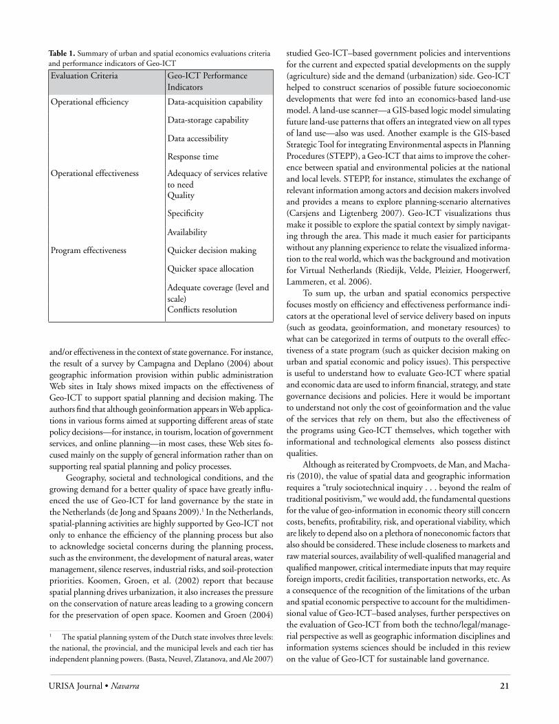
the urBan and SPatIal econoMIcS PerSPectIveThe urban and spatial economics perspective concentrates on the spatial management of cities as an administrative unit. This perspective studies the extent of the geographic, spatial, and eco-nomic phenomena that determine both urban analysis and the formulation and implementation of regional and urban spatial policies, including development, regeneration, housing and prop-erty markets, urban livability, and future urban form (Madanipour, Hull, and Healey 2001). Spatial analysis and urban policy making are conducted generally to determine all the needs of a city region, from transportation infrastructure to biodiversity conservation and local taxation. Table 1 provides a summary of the evaluation criteria and Geo-ICT performance indicators for urban and regional eco-nomic policies. Economists have described operational efficiency as technical or productive efficiency—the use of resources in the most productive and efficient manner achieving maximum possible output from a given set of inputs (Worthington and Dollery 2000).
Operational efficiency for spatial policy making measures Geo-ICT’s capability in acquiring and storing data in an efficient way. This component is comprised of quantifiable measures such as costs and benefits (Huxhold 1991). The second level is opera-tional effectiveness, which measures “how well information needs are satisfied, and what adverse effects are created” (Clapp et al. 1989: 42), including the adequacy of a geoinformation service relative to a need, its coverage, quality, and availability. Finally, indicators of program effectiveness are related to the contribu-tion of Geo-ICT to faster decision making, including in-space allocation, for different types of use of urban space, providing adequate coverage of social services at different levels and scales, as well as improved conflict resolution in service provision (such as land development and reallocation).
Performance indicators become more complex as we move toward the evaluation of the use of Geo-ICT in terms of efficiency Figure 1. A detailed explanation of the research approach
URISA Journal • Navarra 21
and/or effectiveness in the context of state governance. For instance, the result of a survey by Campagna and Deplano (2004) about geographic information provision within public administration Web sites in Italy shows mixed impacts on the effectiveness of Geo-ICT to support spatial planning and decision making. The authors find that although geoinformation appears in Web applica-tions in various forms aimed at supporting different areas of state policy decisions—for instance, in tourism, location of government services, and online planning—in most cases, these Web sites fo-cused mainly on the supply of general information rather than on supporting real spatial planning and policy processes.
Geography, societal and technological conditions, and the growing demand for a better quality of space have greatly influ-enced the use of Geo-ICT for land governance by the state in the Netherlands (de Jong and Spaans 2009).1 In the Netherlands, spatial-planning activities are highly supported by Geo-ICT not only to enhance the efficiency of the planning process but also to acknowledge societal concerns during the planning process, such as the environment, the development of natural areas, water management, silence reserves, industrial risks, and soil-protection priorities. Koomen, Groen, et al. (2002) report that because spatial planning drives urbanization, it also increases the pressure on the conservation of nature areas leading to a growing concern for the preservation of open space. Koomen and Groen (2004)
1 The spatial planning system of the Dutch state involves three levels: the national, the provincial, and the municipal levels and each tier has independent planning powers. (Basta, Neuvel, Zlatanova, and Ale 2007)
studied Geo-ICT–based government policies and interventions for the current and expected spatial developments on the supply (agriculture) side and the demand (urbanization) side. Geo-ICT helped to construct scenarios of possible future socioeconomic developments that were fed into an economics-based land-use model. A land-use scanner—a GIS-based logic model simulating future land-use patterns that offers an integrated view on all types of land use—also was used. Another example is the GIS-based Strategic Tool for integrating Environmental aspects in Planning Procedures (STEPP), a Geo-ICT that aims to improve the coher-ence between spatial and environmental policies at the national and local levels. STEPP, for instance, stimulates the exchange of relevant information among actors and decision makers involved and provides a means to explore planning-scenario alternatives (Carsjens and Ligtenberg 2007). Geo-ICT visualizations thus make it possible to explore the spatial context by simply navigat-ing through the area. This made it much easier for participants without any planning experience to relate the visualized informa-tion to the real world, which was the background and motivation for Virtual Netherlands (Riedijk, Velde, Pleizier, Hoogerwerf, Lammeren, et al. 2006).
To sum up, the urban and spatial economics perspective focuses mostly on efficiency and effectiveness performance indi-cators at the operational level of service delivery based on inputs (such as geodata, geoinformation, and monetary resources) to what can be categorized in terms of outputs to the overall effec-tiveness of a state program (such as quicker decision making on urban and spatial economic and policy issues). This perspective is useful to understand how to evaluate Geo-ICT where spatial and economic data are used to inform financial, strategy, and state governance decisions and policies. Here it would be important to understand not only the cost of geoinformation and the value of the services that rely on them, but also the effectiveness of the programs using Geo-ICT themselves, which together with informational and technological elements also possess distinct qualities.
Although as reiterated by Crompvoets, de Man, and Macha-ris (2010), the value of spatial data and geographic information requires a “truly sociotechnical inquiry . . . beyond the realm of traditional positivism,” we would add, the fundamental questions for the value of geo-information in economic theory still concern costs, benefits, profitability, risk, and operational viability, which are likely to depend also on a plethora of noneconomic factors that also should be considered. These include closeness to markets and raw material sources, availability of well-qualified managerial and qualified manpower, critical intermediate inputs that may require foreign imports, credit facilities, transportation networks, etc. As a consequence of the recognition of the limitations of the urban and spatial economic perspective to account for the multidimen-sional value of Geo-ICT–based analyses, further perspectives on the evaluation of Geo-ICT from both the techno/legal/manage-rial perspective as well as geographic information disciplines and information systems sciences should be included in this review on the value of Geo-ICT for sustainable land governance.
Table 1. Summary of urban and spatial economics evaluations criteria and performance indicators of Geo-ICT
Evaluation Criteria Geo-ICT Performance Indicators
Operational efficiency Data-acquisition capability
Data-storage capability
Data accessibility
Response time
Operational effectiveness Adequacy of services relative to need Quality
Specificity
Availability
Program effectiveness Quicker decision making
Quicker space allocation
Adequate coverage (level and scale) Conflicts resolution

22 URISA Journal • Vol. 25, No. 1 • 2013
the techno/leGal/ManaGerIal PerSPectIveThis perspective looks at the technical, legal, and managerial processes related to the computerization of geoinformation (such as land records, cadastral and topographic maps, historic informa-tion, etc.), the digitization of workflows and business processes in geoinformation organizations, the provision of digital deeds and digital signatures, electronic conveyancing systems, and electronic registration systems. A useful example to understand techno/mana-gerial/legal Geo-ICT can be provided by Land Information Systems (LIS). An LIS has been defined by the International Federation of Surveyors (FIG) as “a tool for legal, administrative, and economic decision making and an aid for planning and development. A land information system consists on the one hand of a database contain-ing spatially referenced land-related data for a defined area and on the other of procedures and techniques for the systematic collec-tion, updating, processing and distribution of data” (FIG 1995).
Lee (1995) has suggested that developing a conceptual data model based on the identified users and information require-ments in order to integrate survey record information into a digital cadastre can be used to develop a typical land administra-tion Web site, which could serve a number of users including citizens (property owners, buyers, sellers, developers, investors), politicians, decision makers, and land specialists and professionals (surveyors, planners, conveyances). Such a dominant approach to the use of Geo-ICT in public administration sees it as a way to maximize government business efficiency and effectiveness par-ticularly related to the delivery of geoinformation, land markets, and location-based services to the public in activities such as land acquisition, subdivision, adjudication, reallocation, assessment, and planning consent and use policies.
An important application of this perspective is expressed by land information systems that address contemporary and future needs of national land administration systems. Zevenbergen (2002) suggests that sustainable land administration systems re-quire the process of recording legally recognized interests of land (ownership and use), including the technical, legal, and manage-rial issues concerning the legal situation of defined units of land. Typically, modeling approaches translate into land information systems practice in the use of specific software development lan-guages and methodologies to achieve the objective of making geo-information a standardizable, formal, and quantitative expression of spatial knowledge. Visual modeling languages such as Unified Modeling Language (UML) are used for specifying, visualizing, constructing, and documenting the artifacts of an LIS software system (Rumbaugh, Jacobson, and Booch 1999). It is a family of design notations that rapidly is becoming a de facto standard software design language for land administration systems. Tu-ladhar (2002) also has suggested that use case models for parcel subdivision processes and dissemination of information show that use cases are excellent for capturing LIS user’s requirements and combined with activity diagrams are promising for realizing e-government services by land administration organizations.
A techno/legal/managerial perspective (see Table 2) can even complement the urban and regional economic perspective. Combining historical land-use information, data on the histori-cal pattern of landscape functions, and the potential of existing structures also is important to evaluate Geo-ICT for sustainable land governance. Van der Molen and Wubbe (2007), for example, elucidate the use of Geo-ICT in e-government with the case study of the Dutch Kadaster’s recent e-land administration initiatives. These include electronic conveyancing, a countrywide deed register, a register of names of rightful claimants, cadastre online and My Cadastre, the authentic register, a one-stop shop for sub-surface infrastructure information, e-services, 24-hour presence, e-mail billing, and the Top 10 NL database. Interestingly, this perspective gives e-land administration a much broader role as a fundamental government infrastructure equivalent to a major highway or railway, although it was originally created on behalf of taxpayers merely for the internal administration of taxation, and, more recently, for titling of land in support of more efficient and effective land markets.
Without these digital facilities, modern governments cannot understand the built environment of cities, manage land effi-ciently, develop area-based land-use policies, or retrieve significant value out of land. Van der Molen and Wubbe (2007) highlight the importance of Geo-ICT for sustainable land governance when the public administration, private sector, and citizens decide on issues where the spatial component is one of the determinants of decisions, such as when there is a need to access relevant spatial information, and could contribute in a meaningful way to the process of spatial decision making. This includes the optimiza-tion of future landscape development based on the quantitative analysis of historical states that can be used for the continuous monitoring of comparable metrics and indices in time series. Time series involve the combination of statistical and spatial analyses to show distinct patterns associated with a change in demographic
Table 2. Summary of techno/legal/managerial evaluation criteria and performance indicators of Geo-ICT
Evaluation Criteria Geo-ICT Performance Indicator
Legal, administrative, and economic decision making; aid for planning and land development
Spatial decision making involving public administration, private sector, and citizens
Support for efficient and effective land markets
Systematic collection, updating, processing, and distribution of data
Maximization of government efficiency and effectiveness in geoinformation-based service delivery
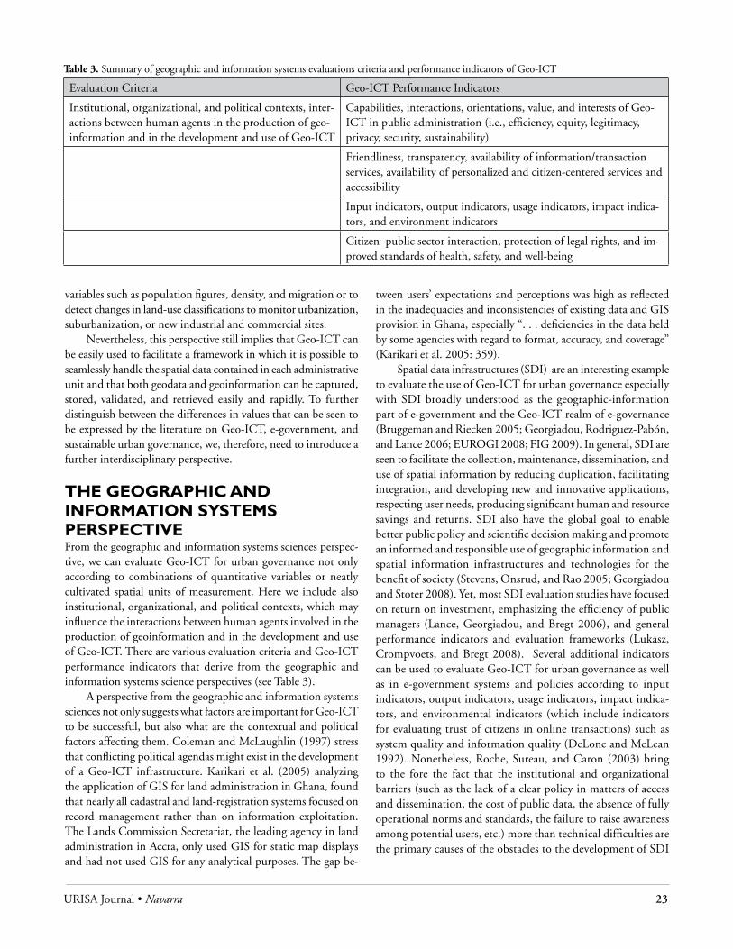
URISA Journal • Navarra 23
variables such as population figures, density, and migration or to detect changes in land-use classifications to monitor urbanization, suburbanization, or new industrial and commercial sites.
Nevertheless, this perspective still implies that Geo-ICT can be easily used to facilitate a framework in which it is possible to seamlessly handle the spatial data contained in each administrative unit and that both geodata and geoinformation can be captured, stored, validated, and retrieved easily and rapidly. To further distinguish between the differences in values that can be seen to be expressed by the literature on Geo-ICT, e-government, and sustainable urban governance, we, therefore, need to introduce a further interdisciplinary perspective.
the GeoGraPhIc and InforMatIon SySteMS PerSPectIveFrom the geographic and information systems sciences perspec-tive, we can evaluate Geo-ICT for urban governance not only according to combinations of quantitative variables or neatly cultivated spatial units of measurement. Here we include also institutional, organizational, and political contexts, which may influence the interactions between human agents involved in the production of geoinformation and in the development and use of Geo-ICT. There are various evaluation criteria and Geo-ICT performance indicators that derive from the geographic and information systems science perspectives (see Table 3).
A perspective from the geographic and information systems sciences not only suggests what factors are important for Geo-ICT to be successful, but also what are the contextual and political factors affecting them. Coleman and McLaughlin (1997) stress that conflicting political agendas might exist in the development of a Geo-ICT infrastructure. Karikari et al. (2005) analyzing the application of GIS for land administration in Ghana, found that nearly all cadastral and land-registration systems focused on record management rather than on information exploitation. The Lands Commission Secretariat, the leading agency in land administration in Accra, only used GIS for static map displays and had not used GIS for any analytical purposes. The gap be-
tween users’ expectations and perceptions was high as reflected in the inadequacies and inconsistencies of existing data and GIS provision in Ghana, especially “. . . deficiencies in the data held by some agencies with regard to format, accuracy, and coverage” (Karikari et al. 2005: 359).
Spatial data infrastructures (SDI) are an interesting example to evaluate the use of Geo-ICT for urban governance especially with SDI broadly understood as the geographic-information part of e-government and the Geo-ICT realm of e-governance (Bruggeman and Riecken 2005; Georgiadou, Rodriguez-Pabón, and Lance 2006; EUROGI 2008; FIG 2009). In general, SDI are seen to facilitate the collection, maintenance, dissemination, and use of spatial information by reducing duplication, facilitating integration, and developing new and innovative applications, respecting user needs, producing significant human and resource savings and returns. SDI also have the global goal to enable better public policy and scientific decision making and promote an informed and responsible use of geographic information and spatial information infrastructures and technologies for the benefit of society (Stevens, Onsrud, and Rao 2005; Georgiadou and Stoter 2008). Yet, most SDI evaluation studies have focused on return on investment, emphasizing the efficiency of public managers (Lance, Georgiadou, and Bregt 2006), and general performance indicators and evaluation frameworks (Lukasz, Crompvoets, and Bregt 2008). Several additional indicators can be used to evaluate Geo-ICT for urban governance as well as in e-government systems and policies according to input indicators, output indicators, usage indicators, impact indica-tors, and environmental indicators (which include indicators for evaluating trust of citizens in online transactions) such as system quality and information quality (DeLone and McLean 1992). Nonetheless, Roche, Sureau, and Caron (2003) bring to the fore the fact that the institutional and organizational barriers (such as the lack of a clear policy in matters of access and dissemination, the cost of public data, the absence of fully operational norms and standards, the failure to raise awareness among potential users, etc.) more than technical difficulties are the primary causes of the obstacles to the development of SDI
Table 3. Summary of geographic and information systems evaluations criteria and performance indicators of Geo-ICT
Evaluation Criteria Geo-ICT Performance Indicators
Institutional, organizational, and political contexts, inter-actions between human agents in the production of geo-information and in the development and use of Geo-ICT
Capabilities, interactions, orientations, value, and interests of Geo-ICT in public administration (i.e., efficiency, equity, legitimacy, privacy, security, sustainability)
Friendliness, transparency, availability of information/transaction services, availability of personalized and citizen-centered services and accessibility
Input indicators, output indicators, usage indicators, impact indica-tors, and environment indicators
Citizen–public sector interaction, protection of legal rights, and im-proved standards of health, safety, and well-being
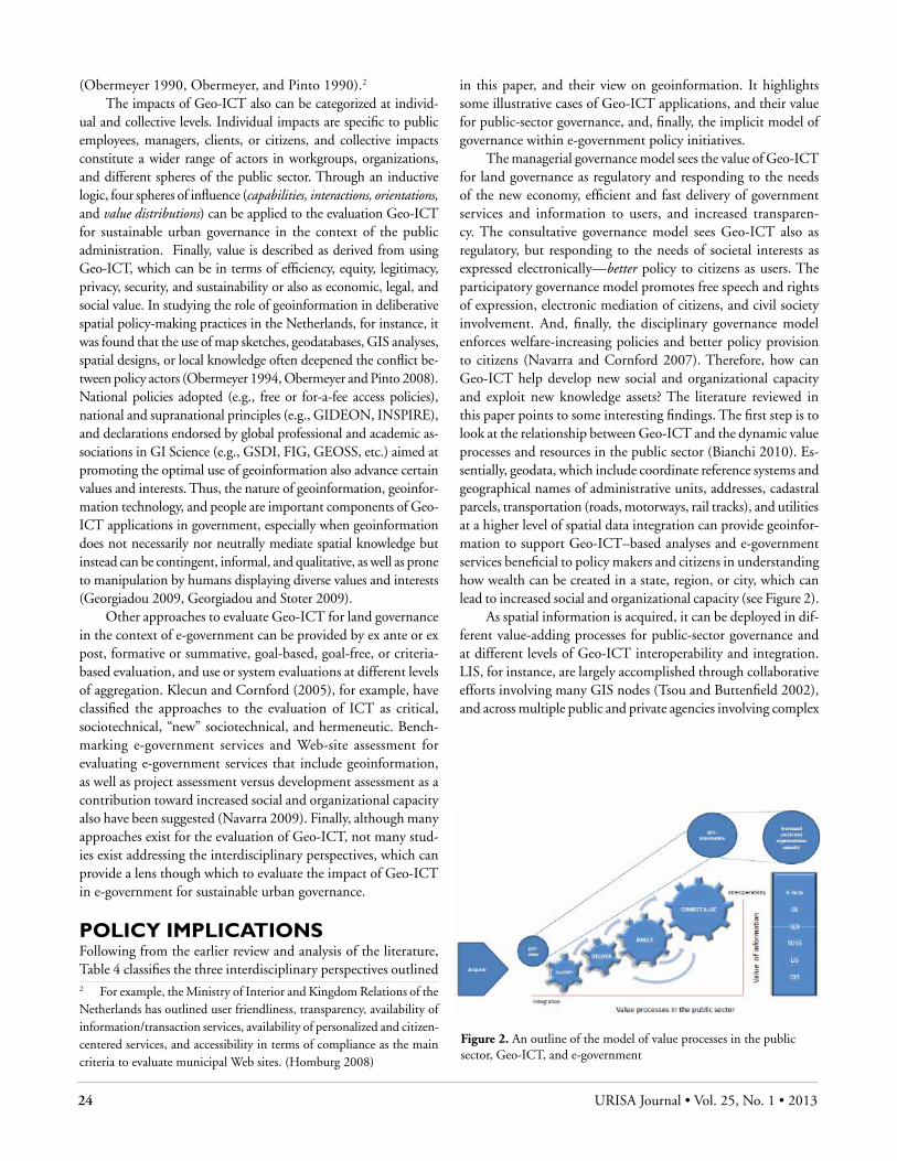
24 URISA Journal • Vol. 25, No. 1 • 2013
(Obermeyer 1990, Obermeyer, and Pinto 1990).2 The impacts of Geo-ICT also can be categorized at individ-
ual and collective levels. Individual impacts are specific to public employees, managers, clients, or citizens, and collective impacts constitute a wider range of actors in workgroups, organizations, and different spheres of the public sector. Through an inductive logic, four spheres of influence (capabilities, interactions, orientations, and value distributions) can be applied to the evaluation Geo-ICT for sustainable urban governance in the context of the public administration. Finally, value is described as derived from using Geo-ICT, which can be in terms of efficiency, equity, legitimacy, privacy, security, and sustainability or also as economic, legal, and social value. In studying the role of geoinformation in deliberative spatial policy-making practices in the Netherlands, for instance, it was found that the use of map sketches, geodatabases, GIS analyses, spatial designs, or local knowledge often deepened the conflict be-tween policy actors (Obermeyer 1994, Obermeyer and Pinto 2008). National policies adopted (e.g., free or for-a-fee access policies), national and supranational principles (e.g., GIDEON, INSPIRE), and declarations endorsed by global professional and academic as-sociations in GI Science (e.g., GSDI, FIG, GEOSS, etc.) aimed at promoting the optimal use of geoinformation also advance certain values and interests. Thus, the nature of geoinformation, geoinfor-mation technology, and people are important components of Geo-ICT applications in government, especially when geoinformation does not necessarily nor neutrally mediate spatial knowledge but instead can be contingent, informal, and qualitative, as well as prone to manipulation by humans displaying diverse values and interests (Georgiadou 2009, Georgiadou and Stoter 2009).
Other approaches to evaluate Geo-ICT for land governance in the context of e-government can be provided by ex ante or ex post, formative or summative, goal-based, goal-free, or criteria-based evaluation, and use or system evaluations at different levels of aggregation. Klecun and Cornford (2005), for example, have classified the approaches to the evaluation of ICT as critical, sociotechnical, “new” sociotechnical, and hermeneutic. Bench-marking e-government services and Web-site assessment for evaluating e-government services that include geoinformation, as well as project assessment versus development assessment as a contribution toward increased social and organizational capacity also have been suggested (Navarra 2009). Finally, although many approaches exist for the evaluation of Geo-ICT, not many stud-ies exist addressing the interdisciplinary perspectives, which can provide a lens though which to evaluate the impact of Geo-ICT in e-government for sustainable urban governance.
PolIcy IMPlIcatIonSFollowing from the earlier review and analysis of the literature, Table 4 classifies the three interdisciplinary perspectives outlined 2 For example, the Ministry of Interior and Kingdom Relations of the Netherlands has outlined user friendliness, transparency, availability of information/transaction services, availability of personalized and citizen-centered services, and accessibility in terms of compliance as the main criteria to evaluate municipal Web sites. (Homburg 2008)
in this paper, and their view on geoinformation. It highlights some illustrative cases of Geo-ICT applications, and their value for public-sector governance, and, finally, the implicit model of governance within e-government policy initiatives.
The managerial governance model sees the value of Geo-ICT for land governance as regulatory and responding to the needs of the new economy, efficient and fast delivery of government services and information to users, and increased transparen-cy. The consultative governance model sees Geo-ICT also as regulatory, but responding to the needs of societal interests as expressed electronically—better policy to citizens as users. The participatory governance model promotes free speech and rights of expression, electronic mediation of citizens, and civil society involvement. And, finally, the disciplinary governance model enforces welfare-increasing policies and better policy provision to citizens (Navarra and Cornford 2007). Therefore, how can Geo-ICT help develop new social and organizational capacity and exploit new knowledge assets? The literature reviewed in this paper points to some interesting findings. The first step is to look at the relationship between Geo-ICT and the dynamic value processes and resources in the public sector (Bianchi 2010). Es-sentially, geodata, which include coordinate reference systems and geographical names of administrative units, addresses, cadastral parcels, transportation (roads, motorways, rail tracks), and utilities at a higher level of spatial data integration can provide geoinfor-mation to support Geo-ICT–based analyses and e-government services beneficial to policy makers and citizens in understanding how wealth can be created in a state, region, or city, which can lead to increased social and organizational capacity (see Figure 2).
As spatial information is acquired, it can be deployed in dif-ferent value-adding processes for public-sector governance and at different levels of Geo-ICT interoperability and integration. LIS, for instance, are largely accomplished through collaborative efforts involving many GIS nodes (Tsou and Buttenfield 2002), and across multiple public and private agencies involving complex
Figure 2. An outline of the model of value processes in the public sector, Geo-ICT, and e-government
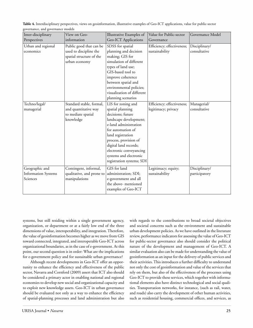
URISA Journal • Navarra 25
systems, but still residing within a single government agency, organization, or department or at a fairly low end of the three dimensions of value, interoperability, and integration. Therefore, the value of geoinformation becomes higher as we move from GIS toward connected, integrated, and interoperable Geo-ICT across organizational boundaries, as in the case of e-government. At this point, our second question is in order: What are the implications for e-government policy and for sustainable urban governance?
Although recent developments in Geo-ICT offer an oppor-tunity to enhance the efficiency and effectiveness of the public sector, Navarra and Cornford (2009) assert that ICT also should be considered a primary actor in enabling national and regional economies to develop new social and organizational capacity and to exploit new knowledge assets. Geo-ICT in urban governance should be evaluated not only as a way to enhance the efficiency of spatial-planning processes and land administration but also
Table 4. Interdisciplinary perspectives, views on geoinformation, illustrative examples of Geo-ICT applications, value for public-sector governance, and governance models
Inter-disciplinary Perspectives
View on Geo-information
Illustrative Examples of Geo-ICT Applications
Value for Public-sector Governance
Governance Model
Urban and regional economics
Public good that can be used to discipline the spatial structure of the urban economy
SDSS for spatial planning and decision making; GIS for simulation of different types of land use; GIS-based tool to improve coherence between spatial and environmental policies; visualization of different planning scenarios
Efficiency; effectiveness; sustainability
Disciplinary/ consultative
Techno/legal/ managerial
Standard stable, formal, and quantitative way to mediate spatial knowledge
LIS for zoning and spatial planning decisions; future landscape development; e-land administration for automation of land registration process, provision of digital land records; electronic conveyancing systems and electronic registration systems; SDI
Efficiency; effectiveness; legitimacy; privacy
Managerial/ consultative
Geographic and Information Systems Sciences
Contingent, informal, qualitative, and prone to manipulations
GIS for land administration; SDI; e-government and all the above- mentioned examples of Geo-ICT
Legitimacy; equity; sustainability
Disciplinary/ participatory
with regards to the contributions to broad societal objectives and societal concerns such as the environment and sustainable urban development policies. As we have outlined in the literature review, performance indicators for assessing the value of Geo-ICT for public-sector governance also should consider the political nature of the development and management of Geo-ICT. A similar evaluation also can be made for understanding the value of geoinformation as an input for the delivery of public services and their activities. This introduces a further difficulty to understand not only the cost of geoinformation and value of the services that rely on them, but also of the effectiveness of the processes using Geo-ICT to provide these services, which together with informa-tional elements also have distinct technological and social quali-ties. Transportation networks, for instance, (such as rail, water, and roads) also carry the development of other human activities, such as residential housing, commercial offices, and services, as

26 URISA Journal • Vol. 25, No. 1 • 2013
well as industrial activities. As a consequence, a perspective on the evaluation of Geo-ICT from the discipline of information systems must be included in the review of the value of Geo-ICT for public-sector governance. The model we presented in Figure 2 is different from any value chain developed for the analysis and evaluation of the activities of private-sector organizations, which often are applied without consideration neither for the differences with respect to public-sector activities nor for the relevance of public-sector processes using Geo-ICT.
There have been many (and indeed still are) initiatives that can be referred to as Geo-ICT around the world, but there has not been any systematic attempt to classify them nor to under-stand Geo-ICT as an e-government policy initiative. Examples of the latter include volunteered geographic information activities (Wikimapia, OpenStreetMap), public initiatives (spatial data infrastructures, geoportals), and private projects (Google Earth, Microsoft Virtual Earth, and other three-dimensional models); these initiatives are producing an overabundance of spatial data while until recently the main challenge in using Geo-ICT–based analyses in the public sector was the lack of availability of spatial data. Such overabundance of spatial information has not yet been aptly put in use to increase the effectiveness of urban governance, particularly for the successful execution of public tasks, for the co-ordination of government agencies and activities, for information and services provision to citizens; for integrated spatial planning and urban management, as well as in providing feedback for the development, planning, and enacting of policies in diverse areas of urban governance for sustainable development including public works, environmental protection, transportation, agriculture, utilities, and public-health management.
A number of key messages emerge from the findings of this review of international experiences and interdisciplinary perspectives on Geo-ICT and their value for urban governance as implications for e-government policy: • What comes to the fore is not only how to quantify the value
of geoinformation for e-government, but to consider what is the contributions and perceived impacts in a dynamic public-sector context;
• For Geo-ICT to make a valuable contribution to societal well-being, a meaningful interdisciplinary approach should be incorporated to develop modalities of evaluation for evaluators, auditors, and public managers not only in the developed world but also in the developing world;
• It is difficult to outline specific metrics to measure the value of geoinformation without considering the presence of multiple sectors, actors, and governance models in the use of Geo-ICT for urban governance.
Combining aptly the interdisciplinary perspectives reviewed in this paper and being aware of the resources and value processes that the introduction of Geo-ICT affect in the public sector will contribute to enhance the understanding of how to evaluate and model public policies as well as the analysis of the potential impacts of e-government on public-management decisions and urban governance not only in terms of efficiency and effectiveness
(such as in economic appraisal, value for money assessment, and impact evaluation), but also for the contribution of Geo-ICT to the development of new knowledge assets, as well as social and organizational capacity and sustainable development.
concludInG reMarKSThe research questions motivating this paper are: What disciplines and approaches help us to understand the value of Geo-ICT for urban governance? What are the implications for public-sector governance and e-government policy?
We have conceptualized and reviewed three interdisciplinary perspectives, their view on geoinformation, illustrative Geo-ICT applications, and value for public-sector governance and gover-nance models for each. Geo-information and Geo-ICT can have an important role to play in e-government transformations and for strengthening urban governance, but more interdisciplinary research needs to be conducted to improve a policy dialogue that can effectively combine the technocentric ideas typical of the highly quantitative geoinformation sciences, leading to gov-ernance models that more often are associated with managerial, disciplinary, and occasionally consultative e-government policy initiatives, with a more qualitative approach based on the poten-tial of Geo-ICT for providing feedback to e-government policy initiatives and participatory policy modeling.
Such a problematization poses challenges to those who set out to develop software and systems, ICT platforms, and infra-structures that can operate within and transform such varied organizational ecologies, but also for policy makers, assessors, and evaluators. This suggests that new challenges lay ahead for the conceptualization of how Geo-ICT for urban governance can be studied as an e-government policy initiative that links together dynamically a variety of actors in new and often tenta-tive networks embodying various interinstitutional relationships and many new creative interdependencies able to increase social and organizational capacity. Geo-ICT and e-government policy initiatives, therefore, should endorse a common future program for the development of a new urban governance architecture that can realize the expectations of citizens and other stakeholders in society. Such a program is about designing information grids able to be exploited across and within new service channels beyond individual organizations and administrative units, potentially transforming also the formulation of public policy as well as the way in which the state presently performs these functions.
About the Author
Diego Navarra (B.Sc., M.Sc., CIMA Cert. B.A., Ph.D.) is a professor (Docente Ordinario) at CERISDI, Italy, and WP visiting professor at the School of Management and Gov-ernance at the University of Twente, The Netherlands. His research and experience include e-government, Geo-ICT, land-information systems, spatial data infrastructures and decision support systems, satellite systems, and three-dimen-
URISA Journal • Navarra 27
sional virtual globes. He is also the founder and director of studionavarra (www.studionavarra.co.uk), a global network of European innovation organizations.
Corresponding Address: Berkeley Square House, Berkeley Square, London, Greater London W1J 6BD, United Kingdom [email protected]
Acknowledgment
The author wishes to thank Her Majesty’s Land Registry (and espe-cially Julie Barry and her staff ) in the United Kingdom for making it possible to present parts of this paper at the 2012 Her Majesty’s Land Registry and United Nations Economic Commission for Europe Conference on Supporting Global Economic Recovery.
References
Akingbade, A., D. D. Navarra, and Y. Georgiadou. 2009. A 10-year review and classification of the geographic information systems impact literature (1998–2008). Nordic Journal of Surveying and Real Estate Research 6: 81-113.
Bailey, K. D. 1994. Typologies and taxonomies: An introduction to classification techniques. Thousand Oaks, CA: Sage.
Basta, C., J. M. M. Neuvel, S. Zlatanova, and B. Ale. 2007. Risk-maps informing land-use planning processes: A survey on the Netherlands and the United Kingdom recent developments. Journal of Hazardous Materials 145 (1-2): 241-49.
Bianchi, C. 2010. Improving performance and fostering account-ability in the public sector through system dynamics model-ling: From an “external” to an “internal” perspective. Systems Research and Behavioral Science 27: 361-84.
Bruggeman, H., and J. Riecken. 2005. Reference data in the Internet—implementation of SDI services as part of e-government. Eleventh EC-GI and GIS Workshop ESDI, Alghero.
Campagna, M., and G. Deplano. 2004. Evaluating geographic information provision within public administration Web sites. Environment and Planning B: Planning and Design 31: 21-37.
Carsjens, G. J., and A. Ligtenberg. 2007. A GIS-based support tool for sustainable spatial planning in metropolitan areas. Landscape and Urban Planning 80 (1-2): 72-83.
Ciborra, C., and D. D. Navarra. 2005. Good governance, de-velopment theory and aid policy: Risks and challenges of e-government in Jordan. Journal of Information Technology for International Development 11 (2).
Clapp, J. L., J. D. McLaughlin, J. G. Sullivan, and A. P. Von-derohe. 1989. Toward a method for the evaluation of mul-tipurpose land information systems. Journal of the Urban and Regional Information Systems Association (URISA) 1: 39-45.
Coleman, D., and J. McLaughlin. 1997. Defining global geospa-tial data infrastructure (GGDI): Components, stakeholders and interfaces. Geomatica 52 (2): 129-43.
Crompvoets, J., E. de Man, and C. Macharis. 2010. Value of spatial data: Networked performance beyond economic rhetoric. International Journal of Spatial Data Infrastructures Research 5: 96-119.
de Jong, J., and M. Spaans. 2009. Trade-offs at a regional level in spatial planning: Two case studies as a source of inspiration. Land Use Policy 26: 368-79.
DeLone, W. H., and E. R. McLean. 1992. Information systems success: The quest for the dependent variable. Information Systems Research 3 (1): 60-95.
EUROGI. 2008. E-government and SDIs: Creating a powerful synergy in the interest of good governance. EUROGI Policy Statement.
FIG. 1995. Statement on the cadastre. Federation of Surveyors by Commission 7 (Cadastre and Land Management). Http://www.fig7.org.uk/.
FIG. 2009. Spatial information for sustainable management of ur-ban areas. FIG Commission 3 Workshop, Mainz.
Georgiadou, Y. 2009. Using geoinformation: From market to a polis perspective. Inaugural Address, International Insti-tute for Geo-Information Science and Earth Observation, Enschede.
Georgiadou, Y., O. Rodriguez-Pabón, and K. T. Lance. 2006. Spatial data infrastructure (SDI) and e-governance: A quest for appropriate evaluation approaches. Journal of the Urban and Regional Information Systems Association URISA) 18 (2): 43-55.
Georgiadou, Y., and J. Stoter, Eds. 2008. SDI for public gover-nance—implications for evaluation research. A multiview framework to assess spatial data infrastructures. Wageningen, RGI, Wageningen University, and Department of Geomatics, University of Melbourne.
Georgiadou, Y., and J. Stoter. 2009. Studying the use of geo-information in government—a conceptual framework. Computers, Environment and Urban Systems 34 (1): 70-78.
Homburg, V. 2008. Understanding e-government. London and New York: Routledge.
Huxhold, W. 1991. An introduction to urban geographic infor-mation systems. Oxford University Press.
Karikari, I., J. Stillwell, and S. Carver. 2005. The application of GIS in the lands sector of a developing country: Challenges facing land administrators in Ghana. International Journal of Geographical Information Science 19: 343-62.
Klecun, E., and T. Cornford. 2005. A critical approach to evalu-ation. European Journal of Information System 14: 229-43.
Koomen, E., and J. Groe. 2004. Evaluating future urbanization patterns in the Netherlands. Forth-fourth Congress of the European Regional Science Association, August 25 to 29, 2004, Porto, Portugal.
28 URISA Journal • Vol. 25, No. 1 • 2013
Koomen, E., J. Groen, J. Borsboom, and H. Scholten. 2002. Modelling the fragmentation of open space: A framework for assessing the impact of land use change on open space. Forty-second Congress of the European Regional Science Association, August 27 to 31, 2002, Dortmund, Germany.
Lance, K. T., P. Y, Georgiadou, and A. Bregt. 2006. Understand-ing how and why practitioners evaluate SDI performance. International Journal of Spatial Data Infrastructures Research (IJSDIR) 1.
Lee, C. 1995. Assessing the value of conceptual modelling: A cost-benefit study. Department of Management Informa-tion Systems, Eller College of Management, University of Arizona. Tucson.
Longhorn, R., and M. Blakemore. 2008. Geographic informa-tion: Value, pricing, production and consumption. Boca Raton: CRC Press.
Lukasz, G., J. Crompvoets, and A. K. Bregt, Eds. 2008. Theoreti-cal introduction to the multiview framework to assess SDIs. A multiview framework to assess spatial data infrastructures. Wageningen, RGI, Wageningen University, and Department of Geomatics, University of Melbourne.
Madanipour, A., A. Hull, and P. Healey. 2001. The governance of place. Ashgate.
Nairn, G. 2009. Spatially enabling society through e-government: A political imperative. GSD11 World Conference—Spatial Data Infrastructrue Convergence, Rotterdam.
Navarra, D., and T. Cornford. 2009. Globalization, networks and governance: Researching global ICT programmes. Govern-ment Information Quarterly 26 (1): 35-41.
Navarra, D. D. 2009. Managing geoinformation systems in the public sector. Enschede: ITC.
Navarra, D. D., and T. Cornford. 2007. The state, democracy and the limits of new public management: Exploring alternative models of e-government. Working Paper Series, Department of Management ISI Group, London School of Economics and Political Science.
NRC. 1993. Toward a coordinated spatial data infrastructure for the nation. Washington, DC.
NRC. 1994. Promoting the national spatial data infrastructure through partnerships. Washington, DC.
NRC. 2001. National spatial data infrastructure partnership programs: Rethinking the focus. Washington, DC.
NRC. 2002. Down to earth: Geographical information for sus-tainable development in Africa. Washington, DC.
NRC. 2007. National land parcel data: A vision for the future. Washington, DC: National Academy Press.
Obermeyer, N. J. 1990. Bureaucratic factors in the adoption of GIS by public organizations: Preliminary evidence from public administrators and planners. Computers, Environ-ment and Urban Systems 14: 261-71.
Obermeyer, N. J. 1994. Spatial conflicts in the Information Age. Journal of the Urban and Regional Information Systems Association (URISA): 1994 Annual Conference Proceed-
ings, Washington, DC, August 8 to 11, 1994, Milwaukee, WI, 269-82.
Obermeyer, N. J., and J. K. Pinto. 1990. Managing geographic information systems. New York: The Guilford Press.
Obermeyer, N. J., and J. K. Pinto. 2008. Managing geographic information systems. New York: The Guilford Press.
Palmer, D., S. Fricskas, and B. Wehrmann. 2009. Towards im-proved land governance. Land Tenure Working Paper 11. Rome, FAO.
Riedijk, A., R. J. v. d. Velde, I. D. Pleizier, T. C. Hoogerwerf, R. J. A. v. Lammeren, et al. 2006. Virtual Netherlands. Geo-visualizations for interactive spatial planning and decision-making: From wow to impact. Vrije Universiteit Amsterdam, Faculteit der Economische Wetenschappen en Bedrijfskunde, Afdeling Ruimtelijke Economie/Spatial Information Labora-tory (SPINlab), Amsterdam, The Netherlands.
Roche, S., K. Sureau, and C. Caron. 2003. How to improve the social utility value of geographic information technologies for the French local governments? A Delphi study. Environ-ment and Planning B: Planning and Design 30 (3): 429-47.
Rodriguez-Pabón, O. 2005. Cadre theorique pour l’evalutation des infrastructures d’information geospatiale. Department Des Sciences Geomatiques, Faculte’ De Foresterie Et De Geomatique. Quebec, Universite Laval. Ph.D.
Rumbaugh, J., I. Jacobson, and G. Booch. 1999. The uni-fied modeling language reference manual. Reading, MA: Addison-Wesley.
Stevens, A. R., H. J. Onsrud, and M. Rao. 2005. Global spatial data infrastructure (GSDI): Encouraging SDI development internationally. ISPRS Workshop on Service and Application of Spatial Data Infrastructure XXXVI (4/W6). Hangtzou, China.
Stoessel, W. 2006. E-government and SDI in Bavaria, Germany. FIG Workshop on e-Governance, Knowledge Management and e-Learning, Budapest.
Thuladar, A. 2002. Developing a framework for cadastre and land registration system in land administration organization. FIG XXII International Congress, Washington, DC.
Tsou, M-H., and B. P. Buttenfield. 2002. A dynamic architecture for distributing geographic information services. Transactions in GIS 6: 355-81.
Van der Molen, P., and M. Wubbe. 2007. E-government and e-land administration as an example: The Netherlands. Sixth FIG Regional Conference: Coastal Areas and Land Administration, Building the Capacity. San Jose, Costa Rica.
Worthington, A. C., and B. E. Dollery. 2000. The debate on Australian federalism: Local government financial inter-relationships with state and commonwealth governments. Australian Journal of Public Administration 59 (4): 12-22.
Zevenbergen, J. 2002. Systems of land registration: Aspects and effects. Netherlands Geodetic Commission (NCG). Delft, University of Delft. Ph.D.
URISA Journal • Bigham, Kang 29
IntroductIonIn the United States, each state has a department of transporta-tion that is tasked with managing, maintaining, and developing state highways. To manage events associated with the highways, transportation data systems have been developed to store rel-evant event information such as pavement types, construction zones, and motor vehicle collisions. The events are stored in a database with location values that are based on distances from measured points along the highway. However, before the advent of geographic information systems (GIS), the benefit of storing the event locations was limited to tabular analyses and paper maps. GIS now can take full advantage of the spatial location information, but significant work is required to match histori-cal measurement systems on the highways to currently available digital street networks. Making this task even more difficult is the fact that many highways have undergone significant realignments over time and known reference markers for the same location on a highway now may have different measurement values. To account for these changes, a linear referencing system (LRS) can be developed from a digital street network.
Linear referencing is the process of storing geographic loca-tions along a linear feature based on their positions relative to measured reference locations. On a highway, intersections and ramps can serve as reference locations to calculate distances to other geographic locations along the length of the highway. Typically, as changes occur to the roadway, new measurements are developed to account for the differences in the length of the route. For example, a bypass could be constructed, increasing the length of a highway that originally traversed through a city. New measure markers are placed along the bypass, but the entire length of the highway is not recalculated to maintain the consistency of previous event locations. In this situation, the beginning and end measurements of the highway remain the same, but the true
distance of the route no longer would be equal to the original distance after the realignment. The ability to incorporate and represent these multiple measurements for the same route is fundamental to the concept of linear referencing and for effective transportation data management.
At the national level, the U.S. Federal Highway Administra-tion (2011) maintains a highway inventory system known as the Highway Performance Monitoring System (HPMS) (http://www.fhwa.dot.gov/policyinformation/hpms.cfm). HPMS contains information on the condition, extent, performance, use, and operating characteristics of the nation’s roadways to accommodate a data-driven process for analysis, planning, and funding alloca-tion purposes. States are required to submit roadway geometry information for all public roads with an associated LRS, but are at different stages of the submission process. The final long-term goal is to have a complete, standardized LRS accessible to the public for all roadways in the country. However, this is an ongoing task and many local agencies or private consulting firms have immediate needs for an LRS to locate different types of events on highways. There also may be a need to build an LRS on a newer or more accurate street network for various projects. Therefore, regardless of a national system, local systems frequently are necessary.
Numerous studies have been devoted to conceptual data modeling of linear referencing systems (Vonderohe and Hepworth 1998, Fletcher et al. 1998, Easa and Chan 1999, Adams et al. 2000, Adams et al. 2001, Scarponcini 2002, Curtin et al. 2007). Of these, most of the transportation-focused LRS literature out-lines data models or best practices for developing new systems (Fletcher et al. 1998, Kiel et al. 1999, Scarponcini 2002, Steiner et al. 2002, Curtin et al. 2007, Zhang et al. 2010). They provide a comprehensive process for building an LRS from scratch and present guidelines for defining the base measuring system that can be used in new data models. However, this literature is of
Building a highway linear referencing System from Preexisting reference Marker Measurements for
transportation data Management
John M. Bigham and Sanghyeok Kang
Abstract: To manage events associated with highways, data systems have been developed to store relevant event information. To reap the full benefits of geographic information system technologies, the relative locations can be integrated into a linear referenc-ing system. The objective of this paper is to present a methodology for building a highway linear referencing system by applying preexisting marker measurements to a digital street network. The system was developed for locating motor vehicle collisions in California and resulted in improved accuracy compared to a previously developed system. Nearly 50 percent of the relative collision locations based on the two different systems were within one meter of each other, but 4.1 percent were greater than 1,000 meters. Differences in collision locations were likely because of improved accuracy for (1) an increased number of reference markers were used, (2) all route realignments were accounted for, and (3) all previously identified errors were corrected.

30 URISA Journal • Vol. 25, No. 1 • 2013
Table 1. Postmiles and prefix letters for realignments. Source: California Highways Numbering Conventions: Postmiles, http://www.cahighways.org/num-postmiles.html, District 5 postmile book
Prefix DescriptionL Overlapping postmilesR RealignmentM Realignment of R mileageN Realignment of M mileageS Spur mileage of original of realign mileageT Temporary connection of original or realign mileageC Commercial lanes paralleling main highwayD Duplication (because of meandering county line)G Reposting duplicate postmile at the end of routeH Realignment of duplication
limited usefulness to researchers or practitioners who must work with a predefined measuring system. Bigham et al. (2009) and Park et al. (2011) developed an LRS by associating preexisting reference markers with a current digital street network. This is a very different procedure, where the goal is to incorporate the past historical modifications into a measuring system to locate recent events in a GIS rather than generating a brand new measuring system. Transportation agencies may not have the luxury to design new measurement protocols when all their legacy data applications and systems rely on the historical system. Therefore, to utilize the benefits of GIS, the labor-intensive process of incorporating the preexisting markers is the only feasible solution.
The objective of this paper is to expand on the work originally developed by Bigham et al. (2009) and Park et al. (2011) and present a methodology for building a highway LRS by associating preexisting reference markers to a modern digital street network. A key component of the new work is the inclusion of all known highway realignments over the entire history of the system rather than only addressing a subset of the largest realignments. The locations of geocoded collisions between the original and new LRS are compared to verify the improved accuracy.
data SourceS
California State Highway Routes California highway data was obtained from StreetMap Pro 2003 and StreetMap North America 2005. StreetMap is a TeleAtlas-based street network that is freely available to ArcGIS software license holders. The California Department of Transportation (Caltrans) originally developed a highway postmile measuring system for routes that were in existence on January 1, 1964 (Cali-fornia Highways, http://cahighways.org). The postmile system is used to maintain all aspects of current roadways and to plan for adjustments or new construction. The California postmile system differs from most other states for it uses a county specific postmile system as opposed to a state-level system. The postmile value of a California highway is not a continuous measure across the whole state; it resets to zero when the highway enters a new county.
When the highway is realigned, those sections are given updated measurements to distinguish from the original measurements. Depending on the type of realignment or previous changes on the roadway, a number of postmile prefix versions as shown in Table 1 are utilized. Transportation data that are associated with the highways follow this established postmile system.
PoStMIle reference MarKerSPostmile reference markers of major intersections, entrance ramps, and exit ramps for all state highways were obtained from the Caltrans Traffic Accident Surveillance and Analysis System (TASAS) and the Traffic and Vehicle Data Systems Unit (avail-able on http://traffic-counts.dot.ca.gov). These reference markers are used to calibrate the LRS. The 21,543 reference markers by location type and data source are summarized in Table 2. County boundary points were generated by creating a spatial overlay of county polygon features on highway line features. Ramps and intersections were manually identified by matching text descrip-tions to line feature end points on the map.
collISIonSAlmost 507,350 fatal or injury collisions occurring on state high-ways in California from 2001 to 2008 were obtained from the Statewide Integrated Traffic Records System (SWITRS, http://www.chp.ca.gov). SWITRS is maintained by the California Highway Patrol and contains all reported collisions in the state. Several elements are included in each report to record the loca-tion of the collision. Collisions occurring on state highways have several additional fields: route number, route direction, postmile, and postmile prefix. An example set of records is shown in Table 3.
Table 2. Data sources of reference markers
Source Location Type Number of MarkersTASAS Intersection/ramp 7,312/10,623ESRI Data and Maps, 2010
County boundary 1,150
Traffic and Vehicle Data Systems Unit
Intersection, ramp, major landmarks
2,458
Total 21,543
Table 3. SWITRS state highway collisions location information example
Route Number
Direction Prefix County Postmile
49 S - EL DORADO 22.998118 W R VENTURA 30.43036 E L TEHAMA 40.320152 W T SANTA CRUZ 3.11978 E N SAN DIEGO 17.680

URISA Journal • Bigham, Kang 31
MethodS
OverviewAn overview of the LRS workflow is shown in Figure 1. Each of the steps is explained in detail in the following subsections. The processes all utilized ArcGIS 10 software from Esri. While some of the techniques and instructions will refer to specific functions in the ArcGIS software, the main concepts are relevant to any linear referencing software.
create routeSThe first step in building a highway LRS is to create routes us-ing highway street segments extracted from a currently available digital street network. This was a semiautomated process that required selecting connecting segments and merging them into a single route/direction for each county. The process is thoroughly explained in Bigham et al. (2009) and Park et al. (2011).
After route features have been extracted and merged, the ArcGIS Create Routes tool can be used to prepare the routes for calibration. An important feature of the tool is the ability to set a coordinate priority location from which measures are accumulated for each route. The coordinate priority typically would be Lower Left for highways accumulating measures from west to east or south to north. This means that measures will be accumulated from the lower left corner of the bounding rectangle for the entire route. However, some routes in California accumulate in the opposite direction and they require using a Lower Right or an Upper Left coordinate priority. The Lower Right routes were not all known for the initial route creation; many were identified only during the error review process and properly recategorized in future route-creation iterations. Routes must be processed in the Create Routes tool in separate sets for each coordinate priority type before being merged into a single set.
Create Duplicate Routes to Account for Highway RealignmentsDifferent measuring systems are required for realigned routes. Although a current street network cannot reflect all the geomet-ric differences in realigned routes, applying different measuring systems to the same geometry can at least approximate the true locations of events on the route. The original work by Bigham et al. (2009) accounted for the largest realignments, such as the example in Figure 2 when a route starts at zero at the county boundary but resets to zero several miles along the route. However, most routes have multiple realignments that each requires separate linear features for proper measurement along the entire length of the route. An example of this concept is shown in Figure 3, with the original route at the bottom having an initial realignment (R) and then a subsequent realignment of the R (M). The final hypothetical combined route is shown at the top. Events occurring in the realigned sections are likely to have the designated R or M prefix and the postmile value will differ from the original route.
We assigned every route a route identifier, called RouteID in this study, concatenated from multiple fields, including the route number, direction, realignment prefix, and county. The RouteID field is used to match events and their corresponding descriptive fields to a particular route, but each route feature also has a per-manent unique numeric identifier in the database. The unique numeric identifier can be used as a reference to accommodate potential route number or geometry changes in the future. As shown in Figure 3, the original route at the bottom was named 80E-ALAMEDA and the realignment (R) and realignment of R (M) were named 80ER-ALAMEDA and 80EM-ALAMEDA, respectively. To accommodate all the potential measuring systems of routes in California, the complete set of routes was copied multiple times to create duplicate sets. Each of the potential
Figure 1. LRS development workflow
Figure 2. 91E-ORANGE realignment
Figure 3. Separate route features for particular prefixes
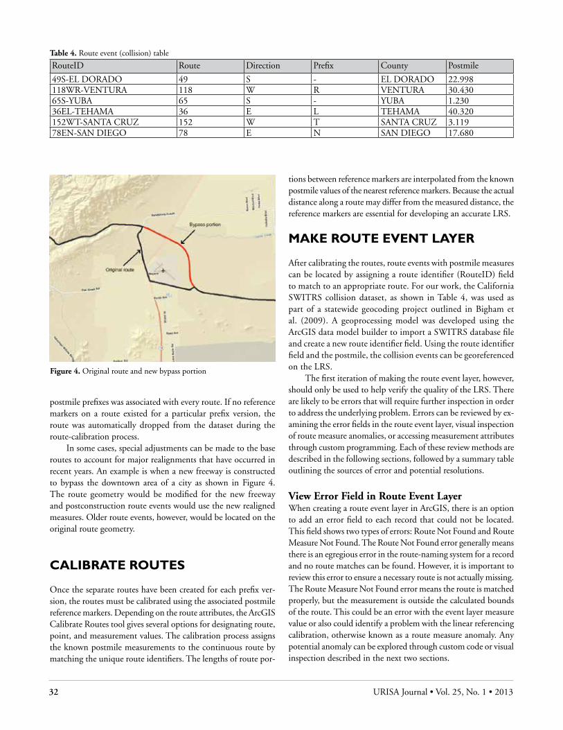
32 URISA Journal • Vol. 25, No. 1 • 2013
postmile prefixes was associated with every route. If no reference markers on a route existed for a particular prefix version, the route was automatically dropped from the dataset during the route-calibration process.
In some cases, special adjustments can be made to the base routes to account for major realignments that have occurred in recent years. An example is when a new freeway is constructed to bypass the downtown area of a city as shown in Figure 4. The route geometry would be modified for the new freeway and postconstruction route events would use the new realigned measures. Older route events, however, would be located on the original route geometry.
calIBrate routeS
Once the separate routes have been created for each prefix ver-sion, the routes must be calibrated using the associated postmile reference markers. Depending on the route attributes, the ArcGIS Calibrate Routes tool gives several options for designating route, point, and measurement values. The calibration process assigns the known postmile measurements to the continuous route by matching the unique route identifiers. The lengths of route por-
tions between reference markers are interpolated from the known postmile values of the nearest reference markers. Because the actual distance along a route may differ from the measured distance, the reference markers are essential for developing an accurate LRS.
MaKe route event layer
After calibrating the routes, route events with postmile measures can be located by assigning a route identifier (RouteID) field to match to an appropriate route. For our work, the California SWITRS collision dataset, as shown in Table 4, was used as part of a statewide geocoding project outlined in Bigham et al. (2009). A geoprocessing model was developed using the ArcGIS data model builder to import a SWITRS database file and create a new route identifier field. Using the route identifier field and the postmile, the collision events can be georeferenced on the LRS.
The first iteration of making the route event layer, however, should only be used to help verify the quality of the LRS. There are likely to be errors that will require further inspection in order to address the underlying problem. Errors can be reviewed by ex-amining the error fields in the route event layer, visual inspection of route measure anomalies, or accessing measurement attributes through custom programming. Each of these review methods are described in the following sections, followed by a summary table outlining the sources of error and potential resolutions.
View Error Field in Route Event Layer When creating a route event layer in ArcGIS, there is an option to add an error field to each record that could not be located. This field shows two types of errors: Route Not Found and Route Measure Not Found. The Route Not Found error generally means there is an egregious error in the route-naming system for a record and no route matches can be found. However, it is important to review this error to ensure a necessary route is not actually missing. The Route Measure Not Found error means the route is matched properly, but the measurement is outside the calculated bounds of the route. This could be an error with the event layer measure value or also could identify a problem with the linear referencing calibration, otherwise known as a route measure anomaly. Any potential anomaly can be explored through custom code or visual inspection described in the next two sections.
Figure 4. Original route and new bypass portion
Table 4. Route event (collision) table
RouteID Route Direction Prefix County Postmile
49S-EL DORADO 49 S - EL DORADO 22.998118WR-VENTURA 118 W R VENTURA 30.43065S-YUBA 65 S - YUBA 1.23036EL-TEHAMA 36 E L TEHAMA 40.320152WT-SANTA CRUZ 152 W T SANTA CRUZ 3.11978EN-SAN DIEGO 78 E N SAN DIEGO 17.680
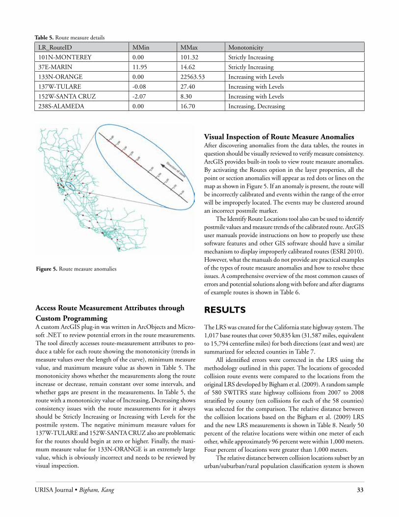
URISA Journal • Bigham, Kang 33
Access Route Measurement Attributes through Custom Programming A custom ArcGIS plug-in was written in ArcObjects and Micro-soft .NET to review potential errors in the route measurements. The tool directly accesses route-measurement attributes to pro-duce a table for each route showing the monotonicity (trends in measure values over the length of the curve), minimum measure value, and maximum measure value as shown in Table 5. The monotonicity shows whether the measurements along the route increase or decrease, remain constant over some intervals, and whether gaps are present in the measurements. In Table 5, the route with a monotonicity value of Increasing, Decreasing shows consistency issues with the route measurements for it always should be Strictly Increasing or Increasing with Levels for the postmile system. The negative minimum measure values for 137W-TULARE and 152W-SANTA CRUZ also are problematic for the routes should begin at zero or higher. Finally, the maxi-mum measure value for 133N-ORANGE is an extremely large value, which is obviously incorrect and needs to be reviewed by visual inspection.
Visual Inspection of Route Measure Anomalies After discovering anomalies from the data tables, the routes in question should be visually reviewed to verify measure consistency. ArcGIS provides built-in tools to view route measure anomalies. By activating the Routes option in the layer properties, all the point or section anomalies will appear as red dots or lines on the map as shown in Figure 5. If an anomaly is present, the route will be incorrectly calibrated and events within the range of the error will be improperly located. The events may be clustered around an incorrect postmile marker.
The Identify Route Locations tool also can be used to identify postmile values and measure trends of the calibrated route. ArcGIS user manuals provide instructions on how to properly use these software features and other GIS software should have a similar mechanism to display improperly calibrated routes (ESRI 2010). However, what the manuals do not provide are practical examples of the types of route measure anomalies and how to resolve these issues. A comprehensive overview of the most common causes of errors and potential solutions along with before and after diagrams of example routes is shown in Table 6.
reSultS
The LRS was created for the California state highway system. The 1,017 base routes that cover 50,835 km (31,587 miles, equivalent to 15,794 centerline miles) for both directions (east and west) are summarized for selected counties in Table 7.
All identified errors were corrected in the LRS using the methodology outlined in this paper. The locations of geocoded collision route events were compared to the locations from the original LRS developed by Bigham et al. (2009). A random sample of 580 SWITRS state highway collisions from 2007 to 2008 stratified by county (ten collisions for each of the 58 counties) was selected for the comparison. The relative distance between the collision locations based on the Bigham et al. (2009) LRS and the new LRS measurements is shown in Table 8. Nearly 50 percent of the relative locations were within one meter of each other, while approximately 96 percent were within 1,000 meters. Four percent of locations were greater than 1,000 meters.
The relative distance between collision locations subset by an urban/suburban/rural population classification system is shown
Table 5. Route measure details
LR_RouteID MMin MMax Monotonicity
101N-MONTEREY 0.00 101.32 Strictly Increasing
37E-MARIN 11.95 14.62 Strictly Increasing
133N-ORANGE 0.00 22563.53 Increasing with Levels
137W-TULARE -0.08 27.40 Increasing with Levels
152W-SANTA CRUZ -2.07 8.30 Increasing with Levels
238S-ALAMEDA 0.00 16.70 Increasing, Decreasing
Figure 5. Route measure anomalies
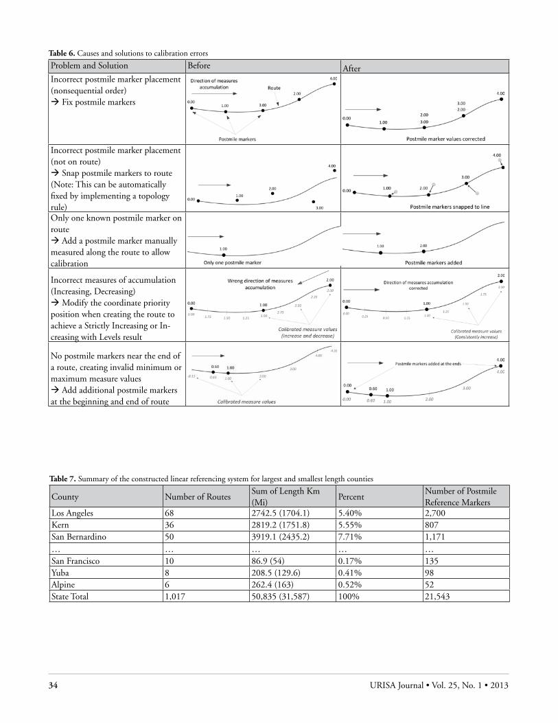
34 URISA Journal • Vol. 25, No. 1 • 2013
Table 6. Causes and solutions to calibration errors
Problem and Solution Before AfterIncorrect postmile marker placement (nonsequential order)à Fix postmile markers
Incorrect postmile marker placement (not on route)à Snap postmile markers to route (Note: This can be automatically fixed by implementing a topology rule)Only one known postmile marker on routeà Add a postmile marker manually measured along the route to allow calibration
Incorrect measures of accumulation (Increasing, Decreasing)à Modify the coordinate priority position when creating the route to achieve a Strictly Increasing or In-creasing with Levels result
No postmile markers near the end of a route, creating invalid minimum or maximum measure valuesà Add additional postmile markers at the beginning and end of route
Table 7. Summary of the constructed linear referencing system for largest and smallest length counties
County Number of RoutesSum of Length Km (Mi)
PercentNumber of Postmile Reference Markers
Los Angeles 68 2742.5 (1704.1) 5.40% 2,700Kern 36 2819.2 (1751.8) 5.55% 807San Bernardino 50 3919.1 (2435.2) 7.71% 1,171… … … … …San Francisco 10 86.9 (54) 0.17% 135Yuba 8 208.5 (129.6) 0.41% 98Alpine 6 262.4 (163) 0.52% 52State Total 1,017 50,835 (31,587) 100% 21,543

URISA Journal • Bigham, Kang 35
in Table 9. Nearly 70 percent of urban collisions were adjusted by less than one meter, while only 44 percent of rural collisions were geocoded that closely. Rural areas contributed to most of the larger differences, with approximately 25 percent of collision locations adjusted more than 100 meters.
dIScuSSIon
The LRS is essential for locating the approximately 40 percent of collisions in California that occur on state highways. Standard intersection-based or address-based geocoding procedures are not able to accurately locate events along highways, especially near large freeway interchanges. These interchanges have multiple crossings that also can vary by the direction of travel, making it unfeasible for a geocoding process to match to a basic intersection name. Also, a recorded intersection on a highway collision report may not actually be a true intersection for it could represent an overpass or a dead-end street that stops at the freeway. Without the LRS, a significant portion of highway collisions could not be geocoded.
The LRS developed in this study resulted in improved accuracy for locating events along the routes compared to the original Bigham et al. (2009) LRS. Differences in collision event locations shown in Table 8 were presumed to be due to improved accuracy based on several factors: (1) an increased number of postmile reference markers were used, (2) all route realignments were accounted for, and (3) all identified LRS errors were cor-rected. The third factor is especially important for the correction of LRS errors alleviated the need for further manual checks to
verify the location of each randomly selected collision. Overall, the most significant improvements occurred along rural routes. Any correction or addition of postmile markers in a rural area impacted a larger portion of a route because of the infrequency of the postmile markers. A rural route may have 50 miles between postmile markers, while an urban route could have a marker every single mile. Thus, when comparing to the original Bigham et al. (2009) LRS, 5.3 percent of rural locations had greater than a 1,000-meter difference, while urban locations were always less than 1,000 meters.
The greater volume of route events in urban areas also sim-plifies visual inspections of the routes. Long portions or rural routes lacking route events would not raise any red flags, but the same situation in urban areas is easily recognizable and requires further investigation. This need for manual visual inspections is an inherent drawback but is necessary to identify errors that do not break the rules of the LRS. For example, an incorrectly located reference marker with a postmile value that falls within the range of the nearest reference markers on either side would not register as an error. However, by incorporating more reference markers and resolving all known errors, the reliance on visual inspections is greatly decreased.
LRS development from preexisting reference markers also is discussed by Park et al. (2011) based on their work for the Korean expressway system. However, there are major differences between the Korean expressway system and the California state highway system. First of all, the sheer size difference between the roadway systems is enormous, with approximately 26,000 kilometers in California compared to only 3,350 kilometers in
Table 8. Distance differences between original LRS collision locations (Bigham et al. 2009) and new LRS
Distance Difference Count Percent Cumulative Count Cumulative Percentage
Less than 1 m 289 49.8% 289 49.8%
1–10 m 63 10.9% 352 60.7%
10–100 m 107 18.4% 459 79.1%
100–1,000 m 97 16.7% 556 95.9%
Greater than 1,000 m 24 4.1% 580 100.0%
Total 580 100.0%
Table 9. Distance differences by population categorization per SWITRS population value for each collision. (Rural: less than 10,000; Suburban: between 10,000 and 100,000; Urban: greater than 250,000)
Area Less Than 1 M 1–10 M 10–100 M 100–1,000 MGreater Than 1,000 M
Total
Rural 165 (43.7%) 40 (10.6%) 79 (20.9%) 74 (19.6%) 20 (5.3%) 378 (100%)
Suburban 98 (57.0%) 20 (10.9%) 25 (18.8%) 17 (10.2%) 4 (3.1%) 164 (100%)
Urban 26 (68.9%) 3 (12.2%) 3 (5.4%) 6 (13.5%) 0 (0.0%) 38 (100%)
Total 289 (49.8%) 63(10.9%) 107(18.4%) 97(16.7%) 24(4.1%) 580(100%)

36 URISA Journal • Vol. 25, No. 1 • 2013
South Korea. The size difference is further magnified by the fact that realignments of California highways are required for most routes, essentially doubling or tripling the total length of routes necessary for LRS development. The Korean expressway system currently does not have realignments and construction projects are focused on developing new roadways, while in California, much of the work is focused on maintaining or modifying existing roads. Thus, realignment measures are necessary for the California LRS, while the Korean expressway LRS can avoid this extra layer of complexity. Secondly, the larger size and inclusion of realign-ments in California decreases the feasibility of relying heavily on manual reviews of the LRS. Our methodology included a more systematic error-checking approach that utilized custom code to extract route measurement attributes. These measurements could be summarized and reviewed in a table format instead of being diagnosed during visual inspections. Finally, we were able to address the calibration issues that Park et al. (2011) referred to as a potential software error. The invalid calibration of some routes that resulted in clustered events was due to incorrect co-ordinate priorities.
There is always some degree of uncertainty when establish-ing the true location of a route event on an LRS. The positional accuracy of the street network and the postmile value associated with a record can heavily impact the calculated location. This makes it difficult to systematically quantify the level of accuracy. If the street network slightly deviates from the actual road place-ment in some locations, those discrepancies will be incorporated into the LRS, but this does not indicate a deficiency in the route calibration. There also can be difficulties when reviewing loca-tions of route events that are assigned postmile values based on descriptive location information. For example, the collision data used in our analysis have a postmile value that the department of transportation manually calculates by translating the descrip-tive location information in the police report. However, there is a potential for translation error and the postmile value may not correctly match the descriptive location information. Occasion-ally, the discrepancies are obvious, but other times they cannot be determined without access to the original police report.
concluSIonS
Many transportation agencies have legacy data systems and need to transition to new GIS-based systems. However, they may not have the luxury to define a new measurement system for road network events. Associating preexisting markers with a current digital street network is the best way to incorporate their legacy data into new applications. The described methodology presents an LRS development approach with an emphasis on components that frequently are overlooked. The methodology clearly outlines how to utilize preexisting reference marker measurements, account for route realignments, and identify and resolve route measure anomalies. The resulting LRS can more effectively locate events occurring on sections of highways that have undergone multiple realignments.
The development of an LRS is essential to managing a highway road network system based on relative measurements. Building a complete, accurate system is a major—but manage-able—task that will likely result in future cost savings and allow agencies to take advantage of numerous GIS technologies. An accurate LRS also can lay the foundations for the development of new measurement protocols and ease the transition from an old system. However, specific protocols are needed for updating the LRS because new roadways are continually being built. The fact that multiple departments in an organization may be utilizing the same LRS also emphasizes the need for proper coordination across the entire organization. Newer multilevel LRS management systems now are available to help simplify long-term maintenance and provide access to common applications to maximize the benefit of an LRS.
Acknowledgments
Funding for this research was provided by a grant from the California Office of Traffic Safety through the National Highway Traffic Safety Administration.
About the Authors
John Bigham is the GIS Program Manager at the Safe Trans-portation Research and Education Center (SafeTREC) at the University of California, Berkeley. His background is in GIS design and analysis and he is responsible for an array of GIS work at SafeTREC, including spatial analysis, Web mapping, and database development projects. He currently is the project director for the Transportation Injury Mapping System (TIMS), a Web site that provides tools to view, query, and spatially explore collision data. He previously worked at the Environmental Systems Research Institute (ESRI) as a product engineer.
Corresponding Address: Safe Transportation Research and Education Center University of California, Berkeley 2614 Dwight Way #7374 Berkeley, CA 94720 Phone: (510) 643-1777 Fax: (510) 643-9922 [email protected]
Sanghyeok Kang is a research fellow in the construction management division of the Construction and Economy Research Institute of Korea. He previously worked as an as-sociate specialist at SafeTREC at the University of California, Berkeley. He earned his Ph.D. from the Civil and Environ-mental Engineering Department at Hanyang University in Seoul, Korea. He develops custom Web and desktop GIS
URISA Journal • Bigham, Kang 37
applications at SafeTREC, including linear referencing and geocoding tools.
Corresponding Address: Construction and Economy Research Institute of Korea 11th F. Construction Bldg. 711 Eonjuro, Kangnam-gu Seoul, 135-701 Korea Phone: +82-2-3441-0720 Fax: +82-2-540-1826 [email protected]
References
Adams, T. M., N. Koncz, and A. P. Vonderohe. Functional require-ments for a comprehensive transportation location referenc-ing system. North American Travel Monitoring Exhibition and Conference (NATMEC), Middleton, Wisconsin, August 27 to 31, 2000.
Adams, T. M., N. Koncz, and A. P. Vonderohe. 2001. Guide-lines for the implementation of multimodal transporta-tion location referencing systems. NCHRP Report 460, Transportation Research Board, National Research Council. Washington, DC: National Academy Press.
Bigham, J. M., T. M. Rice, S. Pande, J. Lee, S. H. Park, N. Guti-errez, and D. R. Ragland. 2009. Geocoding police collision report data from California: A comprehensive approach. International Journal of Health Geographics 8 (72).
Curtin, K. M., G. Nicoara, and R. R. Arifin. 2007. A compre-hensive process for linear referencing. Journal of the Urban and Regional Information Systems Association 19 (2): 23-32.
Easa, S., and Y. Chan. 1999. Implementation of linear referenc-ing systems in GIS. Reston, VA: American Society of Civil Engineers, 79-98.
ESRI. 2010. ArcGIS Desktop Help. ESRI. Http://resources.arcgis.com/content/arcgisdesktop/ 10.0/about, December of 2011.
Fletcher, D., J. Espinoza, R. D. Mackoy, S. Gorden, B. Spear, and A. Vonderohe. 1998. The case for a unified linear reference system. Journal of Urban and Regional Information Systems Association 10 (1): 7-11.
Kiel, D., W. Rasdorf, E. Shuller, and R. Poole. 1999. Linear referencing system for North Carolina Department of Trans-portation. Transportation Research Record: Journal of the Transportation Research Board 1660: 108-13.
Park, S. H., J. M. Bigham, S.-Y. Kho, S. Kang, and D.-K. Kim. 2011. Geocoding vehicle collisions on Korean expressways based on postmile referencing. KSCE Journal of Civil En-gineering 15 (8): 1,435-41.
Scarponcini, P. 2002. Generalized model for linear referencing in transportation. GeoInformatica 6 (1): 35-55.
Steiner, R., I. Bejleri, X. Yang, and D.-H. Kim. Improving geocod-ing of traffic crashes using a custom ArcGIS address matching application. Twenty-second Environmental Systems Research Institute (ESRI) International User Conference, San Diego, California, July 8 to 12, 2002.
U.S. Federal Highway Administration. 2011. Highway perfor-mance monitoring system (HPMS). U.S. Department of Transportation. Http://www.fhws.dot.gov/policyinforma-tion/ hpms.cfm.
Vonherhoe, A. P., and T. D. Hepworth. 1998. A methodology for design of measurement systems for linear referencing. Journal of the Urban and Regional Information Systems Association 10 (1): 48-56.
Zhang, J., S. You, L. Chen, and C. Chen. A hybrid approach to segment-type geocoding of New York City traffic data. Pro-ceedings of the First International Conference on Computing for Geospatial Research and Application, Washington, DC, June 21 to 23, 2010.

URISA Journal • Mukherjee 39
IntroductIon
Work on geospatial data has drawn from two important bodies of literature, organization implementation of GIS and critical GIS. Seminal work within both these bodies of literature has examined the implications of social and political contexts on geospatial data creation and use and also its impacts on organizational decision making. Initial work (Budic 1994, 1998) on such issues has drawn from the organizational implementation literature, while latter studies (Harvey 2003, Harvey and Tulloch 2006, Schuurman 2005, 2009) have followed the critical GIS approach. However, within both bodies of literature, very few studies have addressed the area of social construction of geospatial data creation and dissemination (Harvey et al. 1999, Harvey 2003, Harvey and Tulloch 2006, Schuurman 2002, 2005, 2009). Geospatial data creation is the most time-intensive and expensive part of any GIS project. Various aspects related to geospatial data have significant bearing on GIS use, namely data standardization, data currency, data interoperability, and data integration. In a multiuser and multidepartmental environment, these issues have important implications on the success or failure of a GIS project. Nonetheless, very few research studies have examined how such sociopolitical and institutional norms shape the fate of GIS use and implementation.
The main objective of this article is to examine the process of geospatial data creation and use in Dane County, Wisconsin. By applying a synthesized framework that draws from organiza-tion implementation of GIS and critical GIS literature, this study demonstrates how such a process is intertwined with sociopoliti-cal norms, institutional practices, and economical mores of the county. The next objective is to examine the implications of this social construction of geospatial data on Dane County’s spatial
knowledge production process. By using the case of Dane County, this research demonstrates that geospatial creation and use is a multifarious process. For instance, in Dane County, a singular department is the hub of all countywide GIS activities. As a result, countywide GIS use and implementation depends largely on the circumstances surrounding that particular department. These circumstances are, in turn, influenced by the political environ-ment of the county that influences either directly or indirectly the staff, budget allocation, data creation, and other such key decisions that have serious consequences on the support capacity of the department.
The significance of this study is twofold. First, it contributes to calls for an examination of the social and political contexts influencing geospatial data issues (Harvey et al. 1999, Schuurman 2002, 2005). Second, by examining the sociopolitical contexts that influence Dane County’s geospatial data model and the GIS knowledge production challenges it has ultimately posed for the county departments, this study demonstrates that geospatial data creation is a social process surrounded by multiple social, politi-cal, and institutional contexts. By focusing on technical aspects of geospatial data, there is the risk of completely disregarding the richness of the social process surrounding data creation and its bearing on organizational data issues.
lIterature revIew
Studies on organizational GIS have mainly drawn attention to planning agencies and local government organizations, for these organizations were the foremost users of GIS. Such studies give invaluable insights on geospatial data creation and use (Campbell 1991, Huxhold 1993, Budic 1994). According to these studies, effective GIS knowledge production hinges on data accuracy,
Sociopolitical contexts and Geospatial data—the case of dane county
Falguni Mukherjee
Abstract: Research on geospatial data has drawn mainly from two bodies of literature, organizational implementation of GIS and critical GIS. The organizational literature provides important insights on organizational implications of geospatial data sharing. Scholars who have used the critical GIS lens provide a thorough understanding of the sociopolitical elements that influ-ence geospatial data creation and use. Various aspects related to geospatial data have significant connections with GIS use and have an important bearing on the process of GIS spatial knowledge production. Very few studies to date have focused on the social and political elements that influence geospatial data decisions. Inspired by pioneering work on geospatial data issues, this article examines the process of geospatial data creation and use in Dane County, Wisconsin. It demonstrates how this process is intertwined with the sociopolitical norms of the county and ultimately shapes the county’s GIS spatial knowledge production. By using the case of Dane County, this research demonstrates that geospatial creation and use is a social process shaped by socio-political and institutional elements within which the process is embedded.

40 URISA Journal • Vol. 25, No. 1 • 2013
data sharing, data standardization, data access, and efficient data infrastructure. GIS users in planning agencies have identified data accuracy, data processing, and data access as the most improved aspects of information quality resulting from GIS use. Studies conducted to explore the possibilities of achieving maximum benefits from GIS use identify a multidepartmental or corporate approach to GIS as a pivotal component of organizational GIS (Croswell 1991; Campbell 1991, 1994; Onsrud and Pinto 1993; Budic 1994; Budic and Godschalk 1996).
A valuable component that determines the success of a multidepartmental GIS is geospatial data. To accomplish a mul-tidepartmental approach, it is imperative for an organization to develop an enterprisewide view of geospatial data and processes. Huxhold (1993) argues that with a strong emphasis on geospatial data sharing and user involvement in the development process, an enterprisewide approach can provide a structured and stan-dardized approach to the traditional top-down philosophy of the past. A multidepartmental GIS has the potential to yield greater organizational benefits by avoiding duplication of efforts for da-tabase development and maintenance. Such a strategy has been found to be the most cost-effective approach. An enterprisewide GIS also ensures that a GIS’s capability to integrate data from dif-ferent sources and handle information sharing is used (Campbell 1991, Campbell and Masser 1995), allowing an organization to capitalize on GIS technology’s full potential.
In some organizations, a centralized group performs the planning, implementation, and support of enterprise GIS data and infrastructure as witnessed in Dane County. In others, core data layers and related infrastructure are administered centrally, while individual departments maintain the data and infrastructure specifically required to meet their unique requirements. There is no single enterprise GIS model that is right for everyone. The optimal architecture, procedures, and governance processes ultimately will depend on the complexity of the organization. However, implementing a corporate GIS is a very complex pro-cess and realizing the benefits is even more difficult. According to Masser and Campbell (1995), some of the biggest hurdles in following a corporate strategy are differences in the level of awareness and spatial data-handling skills and in the inability to achieve agreements over access to information, leadership, data standards, equipment, and training.
A number of issues emerge as geospatial data across organiza-tions are integrated. The skills needed to implement a GIS extend beyond technical capabilities to include managerial and data skills. As suggested by Huxhold (1993), collaboration between users, senior management, elected members, and computer specialists is essential for successful GIS implementation at a multidepart-mental level. It is important to identify the most important data providers and to make arrangements for additional resources for departments that are responsible for maintaining the data. Gener-ally, departments or units responsible for maintaining data begin to incur additional workloads, expenses, and responsibilities, and if they perceive inequity in data maintenance commitments, they are inclined or compelled to minimize their support (Budic and
Pinto 2000), as shown in this research. Openness with regard to data access, minimal proprietary interest in data, and gains ex-pected from data distribution are the quintessential prerequisites to avoid conflict regarding data ownership. Also, a clear indication of the nature of the sharing structure should be available early in the process. Allowing GIS and database interaction to evolve over time without set rules and procedures only invites trouble later in the project.
Another strand of research that provides critical insights on issues related to geospatial data uses the critical GIS lens that em-ploys a notion of social construction in GIS examination. Critical GIS calls for a sociopolitical analysis of GIS spatial knowledge production. The notion of social construction thus implies that GIS technology, like any other technology, is embedded in an intricate web of social relationships and remains surrounded by multiple social contentions (Sheppard 1995, 2005). Work under this research umbrella has explored the multifarious sociopolitical contexts that influence geospatial data use (Harvey 1999, 2003; Schuurman 2002, 2005, 2009; Harvey and Tulloch 2006). Cer-tain studies have focused on issues of geographic data sharing and geographic information infrastructures for local govern-ment organizations (Harvey 1998, 2003; Harvey and Tulloch 2006). Harvey (2003) contends that building spatial database infrastructure is an interagency act and thus is a matter of trust. Harvey and Tulloch have examined the process of data sharing in local governments in the United States and have identified four distinct types of local government data-sharing arrangements that reflect institutional, political, and economic factors (Harvey and Tulloch 2006). Differences in data-sharing arrangements reflect flexibility of local government responses to changes in levels of support, political uncertainties, and resilience of staff. As dem-onstrated in thjs work, data sharing involves significant issues of ownership and control, ultimately involving questions of power.
An area related to geospatial data that has received limited attention within the organizational literature as well as critical GIS literature is semantic interoperability and data standardization. Influential work by Schuurman (2005) and Harvey et al. (1999) shed some much needed light on the sociopolitical contexts that impact such issues. Semantic interoperability is still one of the biggest hurdles that organizations and institutions face during geospatial data access and sharing. Lack of sematic interoper-ability is one of the challenges faced by GIS users in Dane County. To develop future standards for geospatial data sharing and minimize data redundancy, it is imperative to identify and resolve semantic issues. According to Harvey et al. (1999) and Schuurman (2005), much attention has been narrowly focused on the technical hurdles of data standardization and interoper-ability while ignoring the social and political contexts that shape such processes. Standardized data is vital to ensure that databases are multifaceted and transferable between departments and ap-plications. Discussing the significance of the social and political influences on semantic interoperability, Harvey et al. (1999) and Schuurman (2005) explain the contextual implications of simplistic terms such as urban, range, or road and how such
URISA Journal • Mukherjee 41
terms can be interpreted differently in different institutional and sociopolitical contexts. Technical and sociopolitical contexts have a two-way relation. Each has an important connection to the other. As Schuurman (2002) emphasizes, there is no division between the two. Technical issues related to data standardization and interoperability ultimately are associated with social and political contexts, as demonstrated in this study.
However, there remains a dearth of empirically grounded research that has examined the sociopolitical contexts that influ-ence such geospatial data issues and its ultimate implications on organizational GIS knowledge production (Harvey 1999, Schuurman 2002, 2005).
Study area
This study is based on research conducted in Dane County, Wis-consin, from 2006 through 2007. Dane County was one of the earlier adopters of GIS in the state of Wisconsin and over the years has developed a robust countywide GIS system. The county has a long history of collaborating with the local community in initiat-ing GIS applications and is considered a regional leader in the use of GIS. Also, the presence of the state capitol, Madison, and the University of Wisconsin-Madison, a premier land-grant research institute, has conferred unique opportunities and resources in the county. The county played a key role in the development of the multipurpose land information system concept by researchers at the university. The local political contexts that have influenced GIS use in Dane County are very unique. First, the presence of a premier university is a major asset that used the county as a test bed to try new and innovative ideas and technologies. Second, the formation of a statewide program, Wisconsin Land Information Program, in the 1980s provided a boost to countywide GIS use.
The county’s GIS activities are attributed to the formation of this program and have been uniquely shaped by it over the years. In accordance with the program requisites, the county established a land information office (LIO), which has evolved into a well-established local and regional resource for geographic and land information services. This office is also the GIS hub of the county. All countywide GIS-related activities are administered and managed by the LIO. The LIO’s GIS activities have been influenced by federal grants, the Wisconsin Land Information Program, research grants, and projects at the university, as well as state and county executive mandates. In the recent past, the local political contexts at Dane County have changed because of various internal and external influences that have impacted countywide GIS use. Dane County’s GIS spatial knowledge production has been reported by a few researchers (Ventura et al. 2003, Ventura 2006, Harvey and Tulloch 2006, Mukherjee and Ghose 2009). For instance, Ventura (2006) discusses the successful GIS prac-tices of Dane County, and Mukherjee and Ghose (2009) provide a comprehensive and in-depth examination of GIS activities of the county within the context of the county’s political, social, historical, and institutional processes. This research examines the internal and external contextual elements that have shaped the
county’s geospatial data model and its impacts on the county’s contemporary GIS spatial knowledge production.
The research methodology used for this study is a case study research method. Arguably, GIS construction is a highly situated process in which the place, context, and relationship matter. In such instances, a case study approach is particularly appropriate. I used a single case study approach because it allows detailed and comprehensive analysis. Case studies are the preferred strat-egy when “how” or “why” questions are being posed, when the investigator has little control over events, and when the focus is on an individual, group, organizational, social, political, and related phenomenon within some real-life context (Yin 2003). Qualitative methods of data collection such as intensive semis-tructured interviews, document analysis, and direct observation at the field site were employed for this research. Multiple data-collection methods were used to generate multiple chains of evidence, verify data collected from various sources, and generate multiple perspectives on key issues. In addition to data verifica-tion and interpretation, using multiple methods was helpful in filling in gaps that existed in some data sources. Data collection was conducted for two months in the spring of 2007 and for four months during the summer of 2007. Pilot work had been conducted in the summer of 2006 to prepare the groundwork for the primary data collection in 2007. Forty in-depth semis-tructured interviews were conducted with actors from various departments within Dane County who make use of GIS such as the LIO manager; GIS technicians; senior planner; members of the sheriff ’s office, public safety, emergency management, and highway departments; the city of Madison officials; officials within the State Cartographer’s office; private agencies involved in GIS projects; spatial and nonspatial data-providing agencies; university researchers who are involved with Dane County; and officials from the Land Information and Computer Graphics Facility (LICGF) of UW–Madison who are involved in constructing GIS either directly or indirectly. To further gather information, docu-ments were thoroughly analyzed that were produced by the LIO, Dane County, city of Madison, and State Cartographer’s office, UW–Madison. Besides these, administrative reports, newspaper clippings, Web sites of related organizations, and journal articles also were critical sources of data.
The following sections discuss the findings from empiri-cal material collected during the course of research. In the next section, the local sociopolitical contexts in Dane County are discussed followed by a discussion of the impact of these contexts on countywide geospatial data.
local SocIoPolItIcal contextS In dane county
The process of GIS adoption and dissemination in the state of Wisconsin is very unique as demonstrated by studies in the past (Kuhlman 1994, Tulloch et al. 1995, 1996, 1997). In the case of Dane County, the noteworthy factors that influenced this process

42 URISA Journal • Vol. 25, No. 1 • 2013
include institutional, economical, and individual human factors such as interorganizational communication, interorganizational stability, and an array of external and internal factors (Tulloch et al. 1995, Mukherjee and Ghose 2009, 2011). The single most critical sociopolitical context that catapulted Dane County’s GIS use was the creation of a statewide program—the Wisconsin Land Information Program (WLIP)—in the 1990s (Tulloch et al. 1995, Mukherjee and Ghose 2009). This statewide program was the culmination of several years of effort by various key actors in Dane County (Tulloch et al. 1995, Mukherjee and Ghose 2011), which resulted in the creation of the Wisconsin Land Information Board (WLIB) and, subsequently, the WLIP as part of Wisconsin Act 31 and 339, respectively. The main objective of the statewide program was to provide financial support to counties in their efforts toward land-records modernization. This objective was achieved as part of Wisconsin Act 339 by establishing a mechanism for funding both the modernization efforts of counties and the WLIP without using money from the state’s general fund (Tulloch et al. 1997).
As part of this legislation, a proposal was adopted that recom-mended an increase in recording fees at the Registrar of Deeds office that would pay toward land-records modernization. Today, the recording fees at the Registrar of Deeds for any real estate transaction is $7, out of which $5 stays with the county where the fee was generated and $2 goes to the state. The county then uses its portion for various modernization efforts, including GIS activities, while the state redistributes its portion as grants to local governments for land-records initiatives.
However, to participate in the statewide program, counties would have to adhere to certain guidelines. The program guide-lines established the following three qualifying criteria for the funding: establish a land information office (LIO), name a land information officer who works for the state as a point of contact, and develop a land-records modernization plan. Other than the qualifying criteria, the program guidelines are very flexible and have imparted complete independence to the counties regarding the structure and administration of their LIOs. For instance, the land information officer can be an individual or a team selected by the county as its representative to the state responsible for executing the land-records modernization plan. In several coun-ties, the officer also serves in other capacities, such as a register of deeds, surveyor, or land conservationist. Following the program guidelines, the Dane County Land Information Office was established by the Dane County Board of Supervisors (Resolu-tion 295, 1989–1990). The county adopted a management by committee approach, in which administration of county LIO activities is supervised by an oversight committee known as the Land Information Office Advisory Committee (personal com-munication 2007). This committee is composed of five officials who guide the county LIO and make key decisions that influence county GIS functions. Since the Dane County LIO’s inception, its activities have been funded by the mechanism established by the statewide program. The Dane County LIO is the core GIS department of the county that manages and facilitates all internal and external countywide GIS-related activities. This office not
only supports the GIS infrastructure of the county but is also the custodian of all spatial data created by the county. Functions of this office include land-records system modernization planning and implementation, acquiring GIS software and hardware, providing training in various GIS software, providing GIS tech-nical support, assisting with data and application development, assisting county departments in investigating various geospatial technology and equipment, assisting in GIS data acquisition and distribution, creating custom map products, and maintaining the geographic information infrastructure for all county departments.
The local political context resulting from the Wisconsin Land Information Program has shaped Dane County’s GIS knowl-edge production in various ways. First, the funding mechanism established by the statewide program has compelled the county’s GIS activities to be overly dependent on external forces. In Dane County, there is no dedicated budget allocated for GIS activities. All GIS functions depend on real estate transaction fees generated at the Register of Deeds Office. This funding arrangement was set up as part of the statewide program during the early 1990s, when GIS use in Dane County was in its infancy. In addition, the real estate market in Dane County has seen a major slump in recent years leading to a huge decline in real estate transaction fees that are collected by the Register of Deeds, which, in turn, affects LIO funds. A slump in the housing sales has caused a slump in the LIO funds. As a result, the LIO has faced huge funding cutbacks that affected the GIS activities that the office could undertake or support. This has given rise to a variety of geospatial issues. As a result, an overdependence on the real estate market has severely hampered Dane County’s GIS capabilities. The following quote from an interview with a county employee (personal communi-cation summer 2007) demonstrates the economic repercussions on county GIS:
What happened over the years when I think in the light of elected officials that they thought that money would fully fund their operations and they did not need to invest anymore. And that’s a fallacy. I can’t think over the top of my head of a number but the Register of Deeds money for Dane County doesn’t pay for 20 percent to 25 percent of the county’s real GIS operations. To get the remaining fund-ing was a challenge. For very expensive data production we were told to be creative and what we did was put together a partnership. We had to go out and find funding through partnership or partners who have money. We had to look for grant opportunities. The best thing would have been for de-partments to have dedicated GIS staff and dedicated budget.
Second, the flexibility conferred by the program guidelines has led to the LIO’s GIS knowledge production being shaped by influential political members within the county. Historically, the authority concerning key decisions of the LIO was placed in the hands of LIO committee members and the county executive, who direct the office regarding the LIO staff, budget allocation, governance issues, policies, and project priorities. Agendas set by key actors on the LIO committee are particularly important

URISA Journal • Mukherjee 43
in shaping LIO’s GIS activities and, in turn, influence the LIO’s capability of providing GIS services to other departments in Dane County. These agendas then are influenced by the priorities of the committee members and other political actors. Key resources of the LIO have been allocated to other departments to fulfill mandates of key political actors, as mentioned by a staff member (personal interview summer 2007):
The County budget has changed fundamentally. And as budgets tightened up the pressure was on the departments to apply LIO money as kind of individual department budget because of their own desperate budget needs. So what hap-pens is if your elected officials do not understand and say that this is important and we are going to fund this development then you would have something like what happened in Dane County where we were told to find some other funding.
This has had a detrimental effect on LIO’s organizational structure and capacity for GIS knowledge production. For in-stance, in recent years, the LIO has faced several restructurings because of funding cutbacks and internal political influences. When the LIO was first established, the office consisted of five staff members—the LIO manager, two database programmers, and two GIS analysts. However, in light of internal mandates and staff restructuring, the office presently functions with only two GIS analysts. The other staff members either have been transi-tioned to other departments or have been dismissed from their positions. Changes in the structure of the LIO over the years are shown in Figures 1, 2, and 3:
Thus, over the years, the LIO has shrunk in terms of man-power, while GIS demands of the county have increased. As a result, the LIO is compelled to provide to an increased countywide GIS demand with less manpower; this has severely hampered its GIS support capacity, and, in turn, there has been a ripple effect on county geospatial data decisions.
SocIoPolItIcal contextS and county GeoSPatIal data
Design of geospatial data is the key to any GIS endeavor. Decisions made during the design of a spatial data model can potentially have far-reaching repercussions on GIS projects. In a multide-partmental and multiuser environment such as the one in Dane County, it is imperative that the geospatial data is comprehensive enough to cater to a wide range of users and departments. The big-gest hurdle identified by GIS users to successful implementation of GIS projects in public agencies was the lack of standardization in data structure and format that inhibited the transfer and exchange of geospatial data (Croswell 1991), as witnessed in Dane County. Today, a new breed of GIS users has emerged in the county, including emergency management, the sheriff ’s office, and 911 services. These new users face several impediments related to geo-spatial data that, in turn, hinder their GIS knowledge production capabilities. Dane County has a very rich geospatial data model,
albeit geared toward land use and planning. Decisions regarding the geospatial data model design were made by key members of the LIO committee when GIS use was first initiated in the county. Because of the land-use and planning-oriented priorities of the LIO committee members, a significant amount of effort was channeled toward creating parcel-mapping data and tax data rather than toward road centerlines data, which is of greater use to departments such as emergency management and public safety who represent the new GIS user group. As a result, these depart-ments lack comprehensive and good quality data. For example, the county lacks good quality roads centerline data. Because of the lack of understanding and agreement regarding conventions and data standards between these departments and the LIO, the roads centerline data lacks consistency and currency. Design of the data attributes is not in accordance to the requirements of the departments that need the centerline data on a daily basis such as for those employees in public safety, the sheriff ’s office, and 911 services. As mentioned by Richard McVicar (personal com-
Figure 1. Traditional structure of Dane County LIO
Figure 3. Structure of Dane County LIO in the summer of 2007
Figure 2. Structure of Dane County LIO in the summer of 2006

44 URISA Journal • Vol. 25, No. 1 • 2013
munication summer 2007) from the public safety department, the roads centerline data is sufficiently good for parcels and tax data but not for emergency services.
Another issue that these departments face is that of data currency. An example is the sheriff ’s office. The sheriff ’s office is required by the state to create a map of all crashes for a calendar year. When officers investigate a crash, they record the location in a record management system used by the sheriff ’s office. The technical staff then uses that information to create crash maps using ArcView. The method adopted by the staff to create these crash maps is very cumbersome because of the unavailability of appropriate geospatial data. An ideal method to map the crash sites would be to geocode the addresses in ArcView; this would automate the entire process and save staff time. However, to do so, the office needs updated roads centerline data to serve as ref-erence data for the geocoding process. The county lacks reliable roads centerline data. This data is not updated regularly and also lacks consistency in naming conventions. The biggest hurdle for these departments is data currency. Importance of data currency has been emphasized by scholars for efficient GIS knowledge production (Croswell 1991, Budic 1998). In a study conducted by Croswell (1991) that identifies hurdles for public organizations in implementing GIS, lack of organizationwide procedures for updating the GIS database was identified as a major impediment, and this occurs in Dane County. As new infrastructure is built, the information does not get updated in the county’s database in a timely manner. Updating such databases is the LIO’s responsi-bility. However, because of staff restructuring, the office is short-staffed. In addition, project priorities of the LIO do not align with those of the new GIS user group. Thus, a new infrastructure such as a road, a house number, or a street is not included in the countywide geospatial database as soon as the location is recorded, and departments such as the sheriff ’s office and the Department of Public Safety Communications Administration are compelled to work with data that is not current. As mentioned by the opera-tions manager (personal interview summer 2007):
It is a multilevel process. There are cases when a new road is created and it even gets built and somehow the loop was not completed and we did not hear about it. There have been times when we get a 911 call and sure enough we get there and there is a road and building and everything, just we didn’t know about it. Even today the maps the dispatchers are looking at are not up to date.
Another quote by a staff member of the sheriff ’s office also demonstrates the frustration among the new GIS users about the unavailability of geospatial data that meets their needs (personal communication summer 2007):
So where are we going to get this accurate centerline file and what mechanism are we going to keep in place to keep it up-dated when a new subdivision is added? That’s the milestone we are dealing with right now. It’s just getting that rock solid accurate centerline file that we can rely on.
Thus, the new GIS users face considerable challenges to GIS spatial knowledge production, posed by a two-pronged issue. One of the issues is a lean-staffed LIO. And the other is the design of the spatial data model of the county that caters more to the requirements of departments representing the LIO committee members and excludes the new GIS user groups that have recently emerged in the county.
The Dane County LIO was established almost 21 years ago, when GIS use in the county was limited to land use and plan-ning. Except for a few departments such as land conservation, planning, and zoning, most of the other county departments lack GIS expertise by staff. As a result, departments that have recently started using GIS completely depend on the LIO for their geospatial requirements. Their capability for GIS knowledge production is shaped by the LIO’s outreach and support capa-bilities. Because of the lack of support of geospatial data needs, database requirements, or GIS technical support from the LIO, these new GIS users have no option other than to depend on a vendor product or abandon their GIS project. An example is the Department of Public Safety Communications Administration, where there is a clear need for a sophisticated mapping and GIS program (Mukherjee and Ghose 2009). However, because of the lack of understanding and support from the LIO, the department is compelled to depend on a vendor-specific product that fails to meet all their geospatial requirements. As mentioned by the operations manager in response to the department’s choice of a non-ESRI product:
It’s what our vendor sells. My understanding is that there are a lot of ways to buy other products and interface them and connect them to our CAD system (dispatch software) but we decided to purchase whatever product our CAD vendor sold. In my limited understanding the product that is in front of our communicators is not ESRI product. It was mainly us going to our vendor and asking them what you can do for mapping. One thing that is not clear to me is what it would mean for us to be ESRI. I hear we want to be ESRI but I don’t know what that means.
This also poses other challenges related to geospatial data such as data interoperability, data integration, data standardiza-tion, and data currency. For a multidepartmental and multiuser environment such as Dane County, interoperability is the key to reduction in cost and time to data management and in the promo-tion of shared organizational structures. Interoperability is a broad discipline and semantic standardization is one of its components (Harvey et al. 1999, Schuurman 2005). When geospatial data are acquired from a variety of sources, data standardization is very difficult to achieve, which is observed in some of Dane County’s departments. Lack of data standardization has the potential to cost an organization excessive staff time and resources as witnessed in the Department of Public Safety Communications Adminis-tration, which uses a mapping program provided by an external vendor to locate incidents in order to send dispatchers to a scene

URISA Journal • Mukherjee 45
of an emergency. This program is very vendor-specific and works only with the vendor’s dispatch software. The program is very limited in the number of layers, such as contours and orthophotos that can be used. It has very limited GIS capabilities and cannot be integrated with any ESRI product. In addition, the database that is used by the program follows a convention for street names and addresses that differs from the convention that has been used for county data by the LIO. For instance, the format used for spelling and naming the streets is very different from that of the county. The street names have spaces that are not present in the county data. For example, everyone there agrees that the road name is McKenna, but one convention names it Mc Kenna, and the other names it McKenna, generating errors when integrating the data. The vendor’s mapping program also has limitations in terms of field sizes and special characters. Sometimes the road name is accurate, but the street suffix cannot be added because the mapping system does not have enough spaces to include it. As a result, parcel data and tax data of the county do not easily integrate with the vendor’s mapping program being used by the Department of Public Safety Communications Administration.
Yet another issue related to data standardization arises from departments using data from external sources; there is a lack of good quality data that serves their requirements. Different geo-spatial data vendors use different street-naming protocols. The main external sources of data are the U.S. Postal Service (USPS) and AT&T Telephone Company. The telephone company uses one convention for data creation, the post office has a different convention, and the department’s mapping program follows a completely different convention. Thus, there is no standardized system for naming streets and addresses. This is a critical issue because spatial attributes used for query and display depend on how a certain attribute is defined (Schuurman 2002, 2005), further impacting spatial knowledge production. One of the biggest issues arises with street naming. AT&T uses the suffix La for “lane,” while the post office (along with the county) uses the suffix “Ln.” Also, the post office recognizes all types of street and suffixes, while AT&T recognizes only 10 to 20 street suffixes. If AT&T does not recognize a particular street type, “St” is placed at the end of the road name. Thus, there are countless streets that are displayed with the suffix “St” at the end, when in reality the road name has a different suffix that must be manually edited by a staff member so that the road names match the names that appear on the dispatchers’ map. The lack of data standardization creates a high overhead cost for the Department of Public Safety Communications Administration in terms of staff time.
concluSIon
Creation and use of geospatial data revolves around social and political contexts as demonstrated in this study on Dane County, Wisconsin. The majority of studies on geospatial data focus on technical details. Very few studies until recently have delved into the social, political, and institutional elements that influence the
creation and use of geospatial data (Harvey 2003; Schuurman 2002, 2005, 2009; Harvey and Tulloch 2006). Geospatial data are socially constructed. The local political context of Dane County shaped the creation of countywide geospatial data when GIS was first introduced in the county, and subsequently the politi-cal contexts also shaped geospatial data use over the years. GIS knowledge production has thrived in the county, and recently a new group of GIS users has emerged. However, the design of the geospatial data model has had a detrimental effect on their GIS use. Countywide geospatial data use is shaped by two important factors. First is the support and outreach capacity of the LIO, which is the main GIS hub of the county. However, the support and outreach capacity of the LIO also is shaped by the local po-litical and institutional contexts, which, in turn, have shaped the construction of county geospatial data. The second factor is the political atmosphere of the county. GIS knowledge production is influenced by agendas and priorities of key political actors. These local political contexts have posed various data-related issues for GIS users, such as data interoperability, data currency, and data standards. Thus, as witnessed in Dane County, geospatial data and issues related to geospatial data are influenced by factors beyond technical elements. Nonetheless, more comprehensive studies are required to shed further light on the social, political, and institutional contexts that shape geospatial data creation and use.
About the Author
Dr. Falguni Mukherjee is an assistant professor in the Depart-ment of Geography and Geology at Sam Houston State University. She earned her degree in Civil Engineering from India and earned her Ph.D. from the University of Wisconsin–Milwaukee. Her research interests include GIS knowledge construction, critical GIS, and GIS use in the non-Western world.
Corresponding Address: Department of Geography and Geology Sam Houston State University P.O. Box 2148 Huntsville, TX 77341 [email protected]
References
Budic, Z., and J. Pinto. 2000. Information sharing in an interor-ganizational GIS environment. Environment and Planning B: Planning and Design 27 (3): 455-74.
Budic, Z. 1998. The impact of GIS technology. Environment and Planning B 25 (5): 681-92.
Budic, Z., and D. R. Godschalk. 1996. Human factors in adoption of geographic information systems (GIS): A local government case study. Public Administration Review 56 (6): 554-67.
46 URISA Journal • Vol. 25, No. 1 • 2013
Budic, Z. 1994. Effectiveness of geographic information systems in local planning. APA Journal 60 (2): 244-63.
Campbell, H., and I. Masser. 1995. GIS and organizations: How effective are GIS in practice? London: Taylor and Francis.
Campbell, H. 1994. How effective are GIS in practice? A case study of British local government. Geographical Information Systems 8 (3): 309-25.
Campbell, H. 1991. Organizational issues in managing geo-graphic information. In Masser, I., and M. Blakemore, Eds. Handling geographic information. London: Longman, 259-82.
Croswell, P. 1991. Obstacles to GIS implementation and guide-lines to increase the opportunities for success. Journal of the Urban and Regional Information Systems Association 3 (1): 43-56.
Ghose, R. 2007. Politics of scale and networks of association in public participation GIS. Environment and Planning A 39: 1,961-80.
Ghose, R. 2005. The complexities of citizen participation through collaborative governance. Space and Polity 9 (1): 61-75.
Harvey, F. 2003. Developing geographic information infrastruc-tures for local government: The role of trust. Canadian Geographer 47 (1): 28-37.
Harvey, F., and N. Chrisman. 2004. The imbrication of geogra-phy and technology: The social construction of geographic information systems. In Brunn, S., S. Cutter, and J. W. Har-rington, Eds. Technoearth: A social history of geography and technology. Boston: Kluwer Academic Publishers.
Harvey, F., W. Kuhn, H. Pundt, Y. Bishr, and C. Riedemann. 1999. Semantic interoperability: A central issue for sharing geographic information. The Annals of Regional Science 33: 213-32.
Harvey, F., and D. Tulloch. 2006. Local government data sharing: Evaluating the foundations of spatial data infrastructures. International Journal of Geographical Information Science 20 (7): 743-68.
Huxhold, W. 1993. The application of research and development from the information systems field to GIS implementation in local government: Some theories on successful adoption and use of GIS technology. In Masser, I., and H. Onsrud, Eds. Diffusion and use of geographic information technologies. Dordrecht/Boston/London: Kluwer Academic Publishers, 61-76.
Kuhlman, K. 1994. Measuring the influences of land records modernization in Wisconsin counties. University of Wis-consin–Madison, unpublished M.S. thesis.
Mukherjee, F., and R. Ghose. 2009. Complexities in GIS con-struction and spatial knowledge production in Dane County, Wisconsin. Cartography and Geographic Information Sci-ence 36 (4): 299-314.
Mukherjee, F., and R. Ghose. 2011. Tracing the historic trajec-tory of GIS development and its effects on contemporary practices. Journal of Urban Technology 18 (3): 141-58.
Onsrud, H., and J. Pinto. 1993. Evaluating correlates of GIS adoption success and the decision process of GIS acquisition. Journal of the Urban and Regional Information Systems Association 5 (1): 8-39.
Schuurman, N. 2009. Critical GIScience in Canada in the new millennium. The Canadian Geographer 53 (2): 139-44.
Schuurman, N. 2005 Social perspectives on semantic interoper-ability: Constraints on geographical knowledge from a data perspective. Cartographica 40 (4): 47-61.
Schuurman, N. 2002. Flexible standardization: Making interoper-ability accessible to agencies with limited resources. Cartog-raphy and Geographic Information Science 29 (4): 343-53.
Sheppard, E. 2005. Knowledge production through critical GIS: Genealogy and prospects. Cartographica 40 (4): 5-21.
Sheppard, E. 1995. GIS and society: Towards a research agenda. Cartography and Geographic Information Systems 22 (1): 5-16.
Tulloch, D., B. Niemann, S. Ventura, and E. Epstein. 1995. Land records modernization in local governments. Proceedings of the 1995 ESRI User Conference.
Tulloch, D., B. Niemann, S. Ventura, and E. Epstein. 1996. Measuring GIS/LIS progress in local governments: Land records modernization and its outcomes. Proceedings of the 1996 ESRI User Conference.
Tulloch, D., B. Niemann, and E. Epstein. 1997. Assessing the out-comes of MPLIS implementation: Identifying and describing benefits. Proceedings of the 1997 ESRI User Conference.
Tulloch, D. 1999. Theoretical model of multipurpose land information systems development. Transactions in GIS 3 (3): 259-83.
Ventura, S. 2006. Crossing the divide: Penetration of spatial information technologies in middle America. GIS Develop-ment 10 (5): 28-33.
Ventura, S., B. Niemann, T. Sutphin, and R. Chenoweth. 2003. GIS-enhanced land use planning in Dane County, Wiscon-sin. Paper submitted for the NCGIA Specialist Meeting on Empowerment, Marginalization, and Public Participation GIS.
Yin, R. 2003. Case study research: Design and methods. 3rd Ed. Thousand Oaks/London/New Delhi: Sage Publications.

URISA Journal • Sahar, Faust 47
IntroductIon
Building footprints as well as two-dimensional and three-dimen-sional representations of buildings are commonly used within numerous routine civil and military operations. From establishing and managing a GIS system for a city, to urban planning and even high-tech military urban combat training, building footprints are an essential part of many daily functions within the private and public sectors. Local government entities such as counties and cities take advantage of technological advances and enhanced im-age resolution as it becomes available to update their geospatial databases. Even with budget constraints, some managed to update their building data layer as often as four or five times in the past 13 years (Kitsap County 2009, Wellington City 2009), often via extensive manual digitizing work (Pennington et al. 2004). Al-leviating the digitizing effort can greatly improve the extraction procedure at all levels of government and private organizations.
Building extraction from aerial images may encounter several major difficulties that any extraction process, manual or automatic, has to overcome. Parts of the building may be ob-structed from view by surrounding objects and shadows, edges of the building may be fuzzy (owing to similarity to the surrounding surfaces or sun-illumination issues), buildings appear different from different perspectives, and much three-dimensional informa-tion is omitted in two-dimensional images. While challenging at times for human operators, an automatic methodology requires operationalizing the logic of a human operator to distinguish a building from its surroundings.
As we strive to achieve an automatic procedure that over-comes most difficulties while maintaining efficiency, the ap-proach developed and demonstrated in this paper can enhance any automatic or manual extraction methodology. It integrates readily available remote sensing and GIS data along with image-processing techniques to simplify the extraction procedure. By proposing and implementing operational procedures that enhance
the building-extraction process, it will be possible to produce in-ventories that are more accurate and cost-effective than by using existing approaches. Data sources would include aerial photogra-phy and local tax-assessor parcel data. The procedure described in this paper provides quantitative evaluation of a simplified manual extraction that may reduce dramatically the amount of time and effort required during the extraction.
Previous WorkThe great variation in building types and surrounding envi-ronments makes an automatic extraction procedure extremely challenging. Humans take advantage of multiple aspects of the building such as shape, shading, texture, illumination, and spatial arrangement to successfully recognize and extract the building. Moreover, aerial and satellite imagery have inherent spectral and spatial characteristics that greatly affect building appearance. As a result, current extraction methodologies usually focus on a specific type of building and sensor while maximizing automa-tion using image-processing techniques. A plethora of prominent techniques and algorithms have been introduced over the years for building and urban mapping, including edge detection; back-ground discriminant transformation (BDT) (Sohn et al. 2005); Hough transform (Lee et al. 2003, Wei et al. 2004); geometric, photometric, and structural analysis (Muller and Zaum 2005); spectral, structural, and contextual analyses (Jin and Davis 2005); geometric activity features (Chan et al. 2009); classification (Hester et al. 2008); seed growing; and others.
Nevertheless, operators still are indispensable during the feature extraction phase. As a result, many applications use a semiautomatic approach to extract points, lines, areas, and complex objects (Vosselman 1998, Sahar and Krupnik 1999, Kim et al. 2004) while utilizing human judgment capabilities as well as computer power for specific repetitive tasks. A histogram peak selection followed by manual identification and seed grow-ing has been suggested for urban area mapping (Li et al. 2006).
an operational approach for Building extraction from aerial Imagery
Liora Sahar and Nickolas Faust
Abstract: Initial building footprint extraction as well as inventory update are still achieved via manual, labor-consuming digitizing from imagery. An extraction methodology is presented that integrates automatic and manual processes. This inte-gration provides the advantage of a repetitive action accomplished by a computer and superior human decision making. The suggested approach incorporates readily available GIS parcels layers to provide an easily replicable simplification process that can precede any extraction procedure. The results emphasize a great savings in time (and subsequently in cost) by using parcel-based partitioning during the image preprocessing and integrating with current common extraction workflows, including manual digitizing. We present a quantitative comparison between the suggested methodology and both an automatic and a fully manual extraction procedure. The approach shows consistent savings of more than 30 percent in time, extracting buildings for both commercial and residential parcels.
48 URISA Journal • Vol. 25, No. 1 • 2013
Three-dimensional characteristics often require more sophisti-cated analysis and search for cues such as shadows (Huertas and Nevatia 1988, Irvin and McKeown 1989, Wei et al. 2004) or the use of stereo imagery (Xiao et al. 2004, Sohn et al. 2005). Integration of GIS datasets at different stages of the extraction procedure is encouraged as a priori knowledge (Baltsavias 2004, Brenner 2005), support building outline update (Koc and Turker 2005), two-dimensional roof extraction (Duan 2004), and three-dimensional building model generation (Khoshelham 2004).
Localizing the search for the building to a specific region within the image significantly simplified the extraction process. Much effort has been invested into subdividing the image for the purpose of region-based extraction (Ming 2005). Partitioning al-gorithms have applied statistical measures to avoid cutting objects and were followed by manual and/or automated feature extraction processes (Ohlhof et al. 2004, Jiang et al. 2008, Zhengjun et al. 2008, Karantzalos and Argialas 2009).
The methodology as presented introduces a new approach to building footprint extraction that integrates GIS as prior knowledge as well as an easy technique to simplify the partition-ing and localize the building-extraction process. An easy way to partition the image prior to the building-extraction process can tremendously simplify the entire procedure. In this paper, we suggest using graphic parcel layer boundaries to restrict the search to the close proximity of the building. Each parcel is cut through the image to create a smaller search region that contains one or more buildings. We present the methodology as well as encouraging results in the next sections.
MethodoloGy
An easily replicable simplification methodology for building extraction is presented that includes tax-assessor parcel layers. Tax-assessor information is readily available in the United States and is becoming more prominent with the global emergence of Geographic Information Infrastructure (GII) (Loenen and Zevenbergen 2010). Digital parcel layers are becoming available as their value is realized for cadaster, surveying, legal purposes, land management, etc. Tax-assessor information can be used at multiple stages of the extraction process for selection of specific buildings of interest (residential, commercial) as well as for elimi-nating vacant parcels. In the methodology described in this paper, the main use of the parcel geometry is to localize the building area to be followed by a manual or automatic extraction. The manual digitization of buildings following the simplification procedure is referred to as simplified manual. Extraction of buildings from an entire scene, as commonly implemented, is referred to as full manual. We compare the proposed methodology for two distinct types of parcels, residential and commercial. The same commercial buildings are extracted using a full manual, a simpli-fied manual process, and an automatic process. The automatic process is based on the extraction methodology discussed in Sahar et al. (2010). The automatic process entails postextraction “result
cleaning” that has to be taken into consideration. The “cleaning” is achieved via a manual review of the results and encompasses adding buildings that were not extracted and refining extracted building footprints. Residential buildings extraction is compared using fully manual and simplified manual procedures.
The simplified manual procedure provides a pragmatic ap-proach that alleviates the tedious task of manually digitizing any type of buildings from imagery. The initial simplification pro-cedure localizes the extraction to a relatively small area and may precede a manual or automatic extraction procedure. Following is a detailed description of the simplified manual approach and a comparison between this approach and automated and fully manual approaches. Implementing the simplification prior to a manual procedure was a result of extensive testing of an automatic methodology (Sahar 2009). Clearly, an automatic process cannot always imitate and completely replace human logic; thus, the re-search recognizes the situations that require manual efforts. Such efforts, inevitable in certain scenarios, can be greatly enhanced, and consistent reduction in time is observed using the simplified method for both residential and commercial parcels.
reSultS
The testing entails manually identifying and digitizing buildings from one-foot resolution-orthorectified imagery. The goal is to compare the postprocessing of an automatic process with two different manual digitization methodologies: full manual and simplified manual. The testing consisted of three techniques: (1) full manual—digitizing buildings from an aerial image; (2) clean-ing the automatic extraction result; and (3) simplified manual—manual digitization of buildings from precut parcel-sized images. The techniques were evaluated for commercial and residential areas separately. Residential buildings were not evaluated for the second technique because of poor performance of the automatic process for those types of buildings. For quantitative evaluation analysis, the user logs the time it takes to perform each of the steps.
The first step, full manual, provides the reference task, as commonly performed during manual building footprints ex-traction. The result is compared with the “clean” result of the automatic process and the manual digitization from parcel-sized images (simplified manual). The actual measured savings in time and effort by digitizing from parcel-sized images are presented as well as potential aggregated savings.
Test AreaFor the testing, 50 commercial and 50 residential parcels were selected (See Figure 1 in which selected parcels are highlighted in blue). The subset of selected parcels accounts for the sample of parcels used in the automatic process. As a result, the subset included multibuilding parcels (12 parcels), parcels in which buildings were not automatically extracted (7 parcels), nonrect-angular buildings (20 parcels), small parcels (14 parcels), and a variety of gray level color buildings. The residential parcels were

URISA Journal • Sahar, Faust 49
selected to include houses that can be easily and clearly identified and houses that have interfering objects and shadows in their surroundings.
During the digitizing process, the parcel layer, as illustrated in Figure 1, is overlaid on the image. The results are presented in Table 1. The commercial parcels include 50 parcels with 84 digi-tized structures, composed of 825 points (built structures range from four-corner buildings to 29-corner compound building). The residential buildings include 50 structures, composed of 334 points (houses range from four-corner to 12-corner structures).
Table 1 presents the results of the manually digitized build-ings for the scenarios detailed previously. The table includes several quantitative comparisons between the methods. First, three different time measures are provided: (1) the overall time for accomplishing the task is provided; (2) this time is divided by the number of buildings to better evaluate the average time it takes to complete the task per building; and (3) the overall time is divided by the number of corners. The last column provides a measure of discrepancy between the result of a method and the digitized buildings layer. The reference layer for the comparison is the result of digitizing buildings from the full-image scene. The layer was selected as the reference to allow consistency for user decision making during the process as well as a measure of
reference to the currently used method by the industry to digitize buildings. The selected layer is a result of a technique that is not confined or restricted by the parcel layer. Thus, it allows for an analysis of the advantages and disadvantages of using parcels for the manual building extraction. The area discrepancy is measured in percent and is calculated by adding all the differences in area between the two layers and then dividing by the total building area in the reference layer.
coMMercIal BuIldInGS
The first three rows in the table compare three different methods for extracting commercial buildings. The first row provides the results for manually digitizing buildings on an entire image scene. The second row provides the results for the postprocessing of the automatic extraction procedure, mainly “cleaning” the automatic process result. “Cleaning” refers to eliminating segments that are not buildings, merging segments where appropriate, moving or deleting vertices, and fully digitizing buildings that were not extracted. The cleaning is performed on the vector polygon layer overlaid on the full image. The third row provides the results for manually digitizing buildings from parcel-sized images.
Figure 1. Fifty commercial (left) and 50 residential (right) parcels selected for manual digitization
Table 1. Results of manually digitizing building within parcelsQuantitative Evaluation
Building Type and Method Time Time Per Building Time per Corner Average Difference in Area (%)
Commercial—full manual. Manually digitizing a full image
42 min. 30 sec. 3.1 sec. N/A. This is the reference layer.
Commercial— “cleaning.” Automatic extraction result
18.5 min. 13.2 sec. 1.3 sec. 3.35%
Commercial—simplified manual. Manually digitizing parcel-sized images
26 min. 18.5 sec. 1.9 sec. 2.01%
Residential—full manual. Manually digitizing a full image
16 min. 19.2 sec. 2.9 sec. N/A. This is the reference layer.
Residential—simplified manual. Manu-ally digitizing parcel-sized images
11 min. 13.2 sec. 2.0 sec. 7.01%
Figure 2. (Left) commercial buildings and parcels show a wide variety of building sizes; (right) residential buildings and parcels are fairly uniform in size.
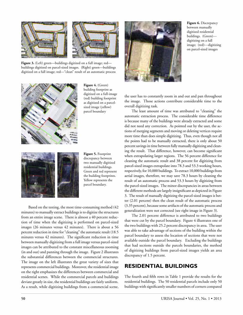
50 URISA Journal • Vol. 25, No. 1 • 2013
Based on the testing, the most time-consuming method (42 minutes) to manually extract buildings is to digitize the structures from an entire image scene. There is almost a 40 percent reduc-tion of time when the digitizing is performed on parcel-sized images (26 minutes versus 42 minutes). There is about a 56 percent reduction in time for “cleaning” the automatic result (18.5 minutes versus 42 minutes). The significant reduction in time between manually digitizing from a full image versus parcel-sized images can be attributed to the constant miscellaneous zooming (in and out) and panning through the image. Figure 2 illustrates the substantial differences between the commercial structures. The image on the left illustrates the great variety of sizes that represents commercial buildings. Moreover, the residential image on the right emphasizes the differences between commercial and residential scenes. While the commercial parcels and buildings deviate greatly in size, the residential buildings are fairly uniform. As a result, while digitizing buildings from a commercial scene,
the user has to constantly zoom in and out and pan throughout the image. Those actions contribute considerable time to the overall digitizing task.
The least amount of time was attributed to “cleaning” the automatic extraction process. The considerable time difference is because many of the buildings were already extracted and some did not need any correction. As pointed out by the user, the ac-tions of merging segments and moving or deleting vertices require more time than does simple digitizing. Thus, even though not all the points had to be manually extracted, there is only about 50 percent savings in time between fully manually digitizing and clean-ing the result. That difference, however, can become significant when extrapolating larger regions. The 56 percent difference for cleaning the automatic result and 38 percent for digitizing from parcel-sized images extrapolate into 78.3 and 53.3 working hours, respectively, for 10,000 buildings. To extract 10,000 buildings from aerial images, therefore, we may save 78.3 hours by cleaning the result of an automatic process and 53.3 hours by digitizing from the parcel-sized images. The minor discrepancies in areas between the different methods are largely insignificant as depicted in Figure 3. The result of manually digitizing the parcel-sized images is bet-ter (2.01 percent) then the clean result of the automatic process (3.35 percent), because some artifacts of the automatic process and generalization were not corrected (see right image in Figure 3).
The 2.01 percent difference is attributed to two buildings that were cut by the parcel boundary. Figure 4 illustrates one of the two buildings with 25.2 percent discrepancy in area. The user was able to take advantage of sections of the building within the parcel boundary to assess the location of sections that were not available outside the parcel boundary. Excluding the buildings that had sections outside the parcels boundaries, the method of digitizing buildings from parcel-sized images yields an area discrepancy of 1.5 percent.
reSIdentIal BuIldInGS
The fourth and fifth rows in Table 1 provide the results for the residential buildings. The 50 residential parcels include only 50 buildings with significantly smaller numbers of corners compared
Figure 3. (Left) green—buildings digitized on a full image; red—buildings digitized on parcel-sized images. (Right) green—buildings digitized on a full image; red—“clean” result of an automatic process
Figure 4. (Green) building footprint as digitized on a full-image (red) building footprint as digitized on a parcel-sized image (yellow) parcel boundary
Figure 5. Footprint discrepancy between two manually digitized residential buildings. Green and red represent the building footprints. Yellow represents the parcel boundary.
Figure 6. Discrepancy between manually digitized residential buildings. (Green)—digitizing on a full image; (red)—digitizing on parcel-sized images

URISA Journal • Sahar, Faust 51
to the commercial parcels. This leads to the considerable difference in manually digitizing the commercial and residential buildings. Moreover, as depicted in Figure 2, the size of residential parcels is fairly uniform and does not require so much zooming in and out during the digitizing process. The results show a consistent significant reduction in time (32 percent) between digitizing from a full image (16 minutes) versus digitizing from parcel-sized im-ages (11 minutes). The major difference between a commercial scene and a residential scene is the degree of decision making required by the user. In a residential scene, many interfering objects and phenomena, such as trees and shadows, can obstruct the building footprint. The user has to invest more time to assess the actual location of the building corner. As a result, even the same user may extract the footprint of the building with great discrepancy. Figure 5 illustrates two such examples, where the same buildings were extracted manually with differences of 46.5 percent (left image) and 15 percent (right image) in area. Unlike the left image (with the 46.5 percent discrepancy), the user was able to take advantage of a clearer shadow area and tree branches to better locate the building footprint on the right image.
Figure 6 illustrates the result of manually digitizing residential houses in clear—free from trees—parcels.
concluSIonS
This paper provides significant insights regarding the use of parcels for the building-extraction process. Using parcels can significantly reduce the time and effort required to extract buildings. They may be utilized as part of an automatic process as well as part of a manual extraction procedure. As presented above, digitizing buildings from parcel-sized images rather than the full image scene may dramatically reduce the extraction time. To avoid cases where the parcel cuts through a building outline, a buffer should be applied around the parcel prior to cutting the images.
Image-partitioning techniques have been researched and developed within the computer science community for diverse applications, including feature extraction. Clearly, an easy and effective method to partition the image prior to the extraction can dramatically simplify the entire procedure. Parcels were shown to simplify the extraction process while maintaining the integ-rity of the buildings. About 15 percent of the commercial and residential houses intersect the parcel boundaries as well as about 50 percent of the high-rise buildings. Buildings that cross parcels lines were found to maintain a significant portion of the buildings within the parcel area. Specific preprocessing recommendations per structure type, for reducing the loss of information such as applying a preprocessing buffer, are discussed in Sahar (2009).
Using parcels to localize the extraction area and eliminate user extraneous operations was shown to be extremely efficient. This contribution is significant as efficient building extraction procedures are required to inventory development, day-to-day management of cities and counties, and for more complex ap-plication such as evaluating damage during an earthquake. All
those applications can greatly benefit from a methodology or procedure that can produce a large percentage of the building inventory or at least considerably reduce the effort.
About the Authors
Liora Sahar received B.Sc. and M.Sc. degrees in geodetic engi-neering from the Israel Institute of Technology (Technion) and a Ph.D. in design computing from the Georgia Institute of Technology, Atlanta. She majored in remote sensing and photogrammetry. She is a GISP and serves as a senior geo-spatial analyst and an adjunct faculty member in the City and Regional Planning Program at the Georgia Institute of Technology. Her teaching research and professional experi-ence include GIS, digital mapping, photogrammetry, remote sensing, feature extraction as well as spatial epidemiology, and emergency preparedness and response.
Georgia Tech Center for Geographic Information Systems 280 Ferst Dr NW Atlanta, GA 30332-0695 [email protected] [email protected]
Nickolas L. Faust received a B.S. in Physics and M.S. in Geophysics from the Georgia Institute of Technology. He served as a prin-cipal research scientist at the Georgia Tech Research Institute in the Electro-Optical Systems Laboratory and is the Associate Director for the Georgia Tech Center for GIS. As head of the Image Analysis and Visualization Branch, he directed efforts at pattern recognition of multispectral image data and terrain analysis of the earth’s terrain. He was a cofounder of the Earth Resources Data Analysis Systems (ERDAS) company and is teaching a remote-sensing course at Georgia Tech. His current interests include the development and use of remote sensing and GIS tools for the analysis of habitat for the last remaining mountain gorillas in Rwanda, Congo, and Uganda.
Georgia Tech Center for Geographic Information Systems 280 Ferst Dr NW Atlanta, GA 30332-0695 [email protected]
References
Baltsavias, E. P. 2004. Object extraction and revision by image analysis using existing geodata and knowledge: Current status and steps towards operational systems. ISPRS Journal of Photogrammetry and Remote Sensing 58 (3-4): 129-51.
Brenner, C. 2005. Building reconstruction from images and laser scanning. International Journal of Applied Earth Observation and Geoinformation 6 (3-4): 187-98.
Chan, J. C-W., R. Bellens, F. Canters, and S. Gautama. 2009. An assessment of geometric activity features for per-pixel classification of urban man-made objects using

52 URISA Journal • Vol. 25, No. 1 • 2013
very high resolution satellite imagery. Photogrammet-ric Engineering and Remote Sensing 75 (4): 397-411. Duan, J., V. Prinet, and H. Lu. 2004. Building extraction in urban areas from satellite images using GIS data as prior information. Proceedings of the 2004 IEEE International, Geoscience and Remote Sensing Symposium, IGARSS 2004, Anchorage, Alaska, 4,762-4.
Hester, B. H., H. I. Cakir, S. A. C. Nelson, and S. Khorram. 2008. Per-pixel classification of high spatial resolution satellite imagery for urban land-cover mapping. Photogrammetric Engineering and Remote Sensing 74 (4): 463-71.
Huertas, A., and R. Nevatia. 1988. Detecting buildings in aerial images. Computer Vision, Graphics and Image Processing 41: 131-52.
Irvin, B. R., and D. M. McKeown, Jr. 1989. Methods for exploit-ing the relationship between buildings and their shadows in aerial imagery. IEEE Transactions on Systems, Man and Cybernetics 19 (6): 1,564-75.
Jiang, N., J. X. Zhang, H. T. Li, and X. G. Lin. 2008. Semiautomatic building extraction from high-resolution imagery based on segmentation. International Workshop on Earth Observation and Remote Sensing Applications, June 2008, Beijing, 1-5.
Jin, X., and C. H. Davis. 2005. Automated building extraction from high-resolution satellite imagery in urban areas using structural, contextual, and spectral information. EURASIP Journal on Applied Signal Processing 14: 2,196-206.
Karantzalos, K., and D. Argialas. 2009. A region-based level set segmentation for automatic detection of man-made objects from aerial and satellite images. Photogrammetric Engineer-ing and Remote Sensing 75 (6): 667-77.
Khoshelham, K. 2004. Building extraction from multiple data sources: A data fusion framework for reconstruction of ge-neric models. The International Archives of the Photogram-metry, Remote Sensing and Spatial Information Sciences, Istanbul, Turkey, 980-6.
Kim, T., Y.-J. Lim, S. Jeong, and K.-O. Kim. 2004. Semiau-tomated map object extraction from 1m resolution space images. The International Archives of the Photogrammetry, Remote Sensing and Spatial Information Sciences, Istanbul, Turkey, 581-7.
Kitsap County. 2009. Footprints for Kitsap County. Http://www,kitsapgov.com/gis/meta data.asp? xml= parcel/foot-prints.shp.xml.
Koc, D. S., and M. Turker. 2005. Automatic building detection from high-resolution satellite images. Proceedings of the Second International Conference on Recent Advances in Space Technologies, Ankara, Turkey, 617-22.
Lee, D. S., J. Shan, and J. S. Bethel. 2003. Class-guided build-ing extraction from IKONOS imagery. Photogrammetric Engineering and Remote Sensing 69 (2): 143-50.
Li, H.-Y., H.-Q. Wang, and C.-B. Ding. 2006. A new solution of automatic building extraction in remote sensing images. IGARSS 2006: IEEE International Conference on GeoScience and Remote Sensing Symposium, Denver, Colorado, 3,790-3.
Loenen, V. B., and J. Zevenbergen. 2010. Assessing geographic
information enhancement. International Journal of Spatial Data Infrastructures Research 5: 244-66.
Ming, D., J. Luo, Z. Shen, and J. Li. 2005. Features-based parcel unit extraction from high-resolution image. Proceedings of the International, Geoscience and Remote Sensing Sympo-sium, IGARSS 2005, Seoul, Korea, 1,875-8.
Muller, S., and D. W. Zaum. 2005. Robust building detection in aerial images. Proceedings of the ISPRS Workshop CMRT 2005, Vienna, Austria, 143-8.
Ohlhof, T., E. Gulch, H. Muller, C. Wiedemann, and M. Torre. 2004. Semiautomatic extraction of line and area features from aerial and satellite images. The International Archives of the Photogrammetry, Remote Sensing and Spatial Information Sciences, Istanbul, Turkey, 2004.
Pennington, H., K. Schmidt, A. Cadieux, and S. Hochart. 2004. Honolulu, Hawaii, building footprint geo-database project: 3D urban visualization. Paper 1693, ESRI proceedings. Http://pro-ceedings.esri.com/library/userconf/ proc04/docs/ pap 1693.pdf.
Sahar, L., and A. Krupnik. 1999. Semiautomatic extraction of building outlines from large-scale aerial images. Photogram-metric Engineering and Remote Sensing 65 (4): 459-65.
Sahar, L. 2009. Using remote-sensing and GIS technology for automated building extraction. Georgia Institute of Technol-ogy, Atlanta, Ph.D. dissertation.
Sahar, L., S. Muthukumar, and S. P. French. 2010. Using aerial imagery and GIS in automated building footprint extrac-tion and shape recognition for earthquake risk assessment of urban inventories. IEEE Transactions on Geoscience and Remote Sensing 48 (9): 3,511-20.
Sohn, H.-G., C.-H. Park, H.-S. Kim, and J. Heo. 2005. 3-D building extraction using IKONOS multispectral images. Proceedings of the International, Geoscience and Remote Sensing Symposium, IGARSS 2005, Seoul, Korea, 1432-34.
Vosselman, G. 1998. Cartographic feature extraction. Bonn, Germany: Institut für Photogrammetrie and Landesvermes-sungsamt NRW.
Wei, Y., Z. Zhao, and J. Song. 2004. Urban building extraction from high-resolution satellite panchromatic image using clustering and edge detection. Proceedings of the 2004 IEEE International, Geoscience and Remote Sensing Symposium, IGARSS 2004, Anchorage, Alaska, 2008-10.
Wellington City, Wellington City Building Footprints Meta-data. 2009. http://koordinates.com/ layer/ 1474/attach-ments/168/.
Xiao, Y., S. K. Lim, T. S. Tan, and S. C. Tay. 2004. Feature extraction using very high-resolution satellite imagery. Pro-ceedings of the 2004 IEEE International, Geoscience and Remote Sensing Symposium, IGARSS 2004, Anchorage, Alaska, 2004-7.
Zhengjun, L., C. Shiyong, and Y. Qin. 2008. Building extraction from high-resolution satellite imagery based on multiscale image segmentation and model matching. International Workshop on Earth Observation and Remote Sensing Ap-plications, EORSA, June 2008. Beijing, 1-7.

URISA Journal • de Armas, Cruz 53
IntroductIon
Geographic information systems (GIS) have become, since the end of the past century, one of the technologies with the broad-est impact on every aspect of modern society, from citizens to governments—especially the latter.
The spatial characterization of both natural and social processes is crucial in many areas of human activity. Thus, the implementation of complex spatial analysis has contributed to the identification of the causes of phenomena such as the emergence of dangerous epidemics, the high proportion of patients suffering from a specific disease, or the increase in crime in a particular residential area.
Moreover, management and optimization of complex trans-portation systems would be unthinkable without the use of spatial distributions of road networks and the location of potential origins and destinations, whether they are ports, warehouses, factories, hospitals, police stations, or fire departments, to name a few.
However, performing the spatial analysis involved in these advances requires having as a prerequisite the coordinates of the objects or phenomena under study. Indeed, it would be impossible to correlate the different sources of chemical contaminants and the cases of a specific respiratory disease detected, for example, unless the exact coordinates of the patients’ homes and the potential sources of contamination are known.
Thus, introducing the powerful tools that GIS technologies provide, with their enormous value to decision-making processes, directly depends on the existence of the location coordinates of objects and phenomena in databases. The spatial information given by geographical coordinates is called explicit georeferenc-ing and, in general, is not available in most operational databases nowadays, particularly those associated with records taken before the appearance of Global Positioning Systems (GPS), which,
undoubtedly, have created a turning point in the availability of spatial information.
Historically, and even today, spatial characterization of objects and phenomena in a large group of activities is based on the use of postal addresses. This has been called implicit geore-ferencing, and although it really represents a spatial variable, it does not serve the purposes described previously, at least directly.
Geocoding is the process of determining the geographic coordinates corresponding to a given postal address or a geo-graphical name. The selection of the postal address closest to given geographic coordinates is known as reverse geocoding.
It is important to have computational approaches to imple-ment geocoding in two variants:• An online service that allows the user to quickly locate
on a map displayed on a computer screen the position corresponding to a textual geographic reference (a postal address or just a geographical name) and
• A computer program that, using the same service, could process a database and convert all postal addresses contained in its records into geographical coordinates.
From a theoretical viewpoint, this complex problem could be regarded as solved. In fact, several GIS software packages ex-ist that provide solutions for implementing geocoding services (MapInfo, ArcGIS, and Oracle).
However, the current situation is not what might be expected, given the existing demand and the technology status because of several factors, including the following:• First, postal addresses have historical and cultural roots, so
these structures may vary considerably from one country to another. This makes geocoding a complex and specific process in every country.
• Second, the geocoding process depends highly on the
deployment of a national Geocoding Service: cuban experience
Carlos José de Armas García and Andrei Abel Cruz Gutiérrez
Abstract: Geocoding is the process of finding the geographic coordinates that correspond to a postal address or a geographic name. Geocoding is performed by comparing the descriptive elements of the address to those present in a reference database. This process can be integrated into numerous applications where a position on a map is required. Then, subsequent spatial analysis of information can be accomplished, such as establishing the relationship between contaminants and the prevalence of certain diseases. This paper presents the results of the process of implementing and deploying a national geocoding service in the context of the spatial data infrastructure for law enforcement of the Republic of Cuba. As an example of the mass application of the service, the statistics of the process of geocoding the national Register of Voters are presented.
PaPerS of PractIce, technIcal rePortS and InduStry noteS

54 URISA Journal • Vol. 25, No. 1 • 2013
existence of a reference database with all the elements that can be part of an address with its correct geographic coordinates. The process of permanently building and updating this database is extremely complex and expensive for several reasons.
Although the situation in developed countries can be con-sidered by no means perfect, in developing countries (or at least in most of them) one cannot speak of any advances regarding geocoding, basically because of the absence of reference databases and even the absence of formal systems of postal address in big residential areas characterized by extreme poverty.
In this paper, the main features of the process of implement-ing and deploying a national geocoding service for law enforce-ment in the Republic of Cuba are presented, as well as the outcome of the process to different applications.
General featureS of GeocodInG
In principle, geocoding requires three elements: address styles and rules (models), the reference database (address elements with their spatial descriptions), and the processing algorithms (Goldberg et al. 2007).
When looking for an address using a geocoder (see Figure 1), structural elements and the attributes of the address are identified (using the rules). These attributes are searched for in the reference data, and candidates with similar attributes to the target address are chosen. Each candidate is assigned a score indicating the simi-larity between what is searched for and what is found, and as an output of the process, the highest scoring candidates are obtained.
Finally, for each candidate, a calculation of the coordinates is made, which, depending on the case, could directly correspond to the coordinates of the element in the reference database (e.g., when the postal address is a corner of two streets) or could require a process of spatial interpolation. In the case of a street segment, for example, the estimation is made based on the ranges of pos-sible numbers for the houses located on each side (odd or even), obtaining the approximate location of the given postal number according to its place within these ranges.
Geocoding services essentially offer three basic functions: online geocoding (given an address, several candidates are ob-tained and the user can choose the best or refine the search), batch geocoding (given an address set, the best candidate for each address is chosen and a set of output is obtained), and reverse geocoding (given the coordinates of a place, the address nearest to that place is obtained).
For batch geocoding addresses stored in a file or a database,
Figure 1. Basic steps of geocoding process
URISA Journal • de Armas, Cruz 55
it is necessary to have a computer program implementing the process of calling the service for a group of records, receiving the results of geocoding, and saving the corresponding values.
Because of the current demand for geocoding, many and varied tools are available worldwide for the implementation of different solutions. For example, a user can freely locate a postal address on an interactive map on Web pages or possibly even obtain complete datasets in different formats to feed geocoding engines supplied by other manufacturers.
Several revisions have been presented in different journals on this issue (see Swift et al. 2008 for a recent and updated compila-tion of alternatives).
In dealing with the deployment of a geocoding service that is national in scope, three components basically are required: definition of the commonly used address models, selection of the software tools implementing the geocoding algorithm, and building of the reference database.
In the following sections, the main features of these compo-nents for the Cuban case are presented. It includes:• Candidates evaluated for each component,• Criteria taken into account for their selection, and• Adjustments made to complete a coherent computer
solution.
All serve as the basis for the deployment of a national geoc-oding service under the conditions of an developing country.
cuBan addreSS ModelS
Postal addresses, as a reference system aimed at locating objects on the earth surface, are the result of a long and complex process through the history of humankind. A basic and intuitive concept of address is a description that includes names and other comple-mentary information pieces, which enable people univocally to identify a place. Under this definition, the following kind of addresses could be recognized:• Postal address. Structural descriptions containing a hierarchy
of places (e.g., country, province, municipality, town, and street) and complementary elements (building number or name, apartment number) used to identify a place. Zip codes are shortcuts to zones or towns and usually are redundant in the address.
• Place name: Denomination of well-known places (points of interest (POI)), whether they are natural or manmade (e.g., buildings).
• Relative address: Description of the location of a place using the name of another place and some complementary information such as distance and/or sense of direction to indicate proximity (for example, a block from the stadium) or the combination of two places (for example, between the bus station and Plaza San Carlos).
The combined use of these kinds of addresses in every country has resulted in specificities; however, in general, the
globalization and convergence processes derived from changes in trade, tourism, migrations, etc., have had an effect on the establishment of universally accepted basic models for urban and rural environments.
Thus, it is very common to find in urban environments an address style made up of the street name (optionally preceded by a prefix) followed by the house number and the elements of the administrative division, for example, municipality, province, country. Additionally, in many cases, the zip code is used to simplify the cumbersome process of sorting letters and packages within the postal industry activity. As a matter of fact, significant effort has been made in different countries to make the use of zip codes compulsory.
Regarding the address system, Cuba, a small Caribbean island (110,000 square kilometers) with 11 million inhabitants, is not an exception to the regularities described previously, both by the existence of the most common models and by the pres-ence of important specific features impossible to ignore in any attempt to establish a national geocoding service. Some of the characteristics identified are:• Low level of standardization of the postal address structure
in the society.• Widespread use of grooves1 in addresses for urban areas, as
an explicit element in the text of the address.• Towns and other rural areas where streets do not have official
names.• Very low use of zip codes.• Diversity of criteria for postal numbering,which can be
associated sometimes with the street and sometimes with the region. Coexistence of different numbering systems corresponding to different historical moments.
• Different forms to place the same prefix and/or suffix on the address text. For example, “Ave 5ta Norte” or “5ta Ave Norte.”
• Abundance of alternate names, for both streets and human settlements.
• Widespread use in city addresses of neighborhood names, usually as a means of disambiguation. To precisely characterize the types of addresses used through-
out the country, the electoral register prepared for the last election process in the country in April of 2010 was used. The participation of the people in the review and updating of the voter lists made them important sources of information about the different address models used in the country and their structures.
This process started with the publication of the local lists of voters, followed by the individual check at the electoral offices of the correctness of the voter names and their addresses. Finally, the corrected lists went back to the national register to upgrade the corresponding database.
1 Attempt to translate the Spanish term entrecalles, which refers to the streets crossing at both corners of a given street. It is widely used in Cuban addresses.

56 URISA Journal • Vol. 25, No. 1 • 2013
The results of this study are shown in Figure 2, where the proportion of different address models among the majority of Cuban homes can be noted.
Based on this classification and also taking into account the expertise of the identification and population office staff, the following models were defined:1. Basic urban model using streets and grooves. This is used in
addresses such as:• Monte # 852 Apto. 3 e/ Arroyo y Matadero, Habana
Vieja, La Habana, Cuba• Ave. 27 No. 4207 e/ 42 y 44, Playa, La Habana, Cuba
In both these cases, the redundant presence of the grooves
(preceded in the text by the sequence “e/”) may be seen, which is stressed in the second case where the grooves are determined by the house number.
This model also has two variants (see the rectangle in the figure): the one used for street corners, for example:• 31 esq. 224, Versalles, Matanzas, Cuba• 23 y 12, Plaza de la Revolución, La Habana, Cuba
Or simply the street name and the house number, like in the model used in other countries.
2. Linear Reference System (LRS), widely used in rural areas, as in the following example. • Carretera a Viñales Km 4, José María Pérez, Pinar del
Río, Pinar del Río, Cuba
3. Model used in a broad group of new settlements built during previous decades where there are no regular road networks. In this case, the building number and the name of the settlement (or a zone within it) is just used as a reference, for example:
• Edif. 674 Apto. 30, Alamar 19, Habana del Este, La Habana
• Ed. Q 66 Apto. 6, Micro 7, Distrito José Martí, Santiago de Cuba, Cuba
4. Model based on the use of the name of a populated settlement or a point of interest. • Finca Los Serafines, Sibanicú, Camagüey, Cuba• Los Mangos, Amancio, Las Tunas, Cuba
Based on these criteria, a rule set was defined to analyze address texts and to extract the key tokens to implement the search.
Two cases were established for this purpose. In the first case, an address is associated with the building model, where the address begins with a prefix indicating the presence of a building (i.e., “EDIF,” “ED,” etc.) and which does not include separators such as “e/,” “esq,” nor “y,” which would mean the existence of a street.
In the other case, an address is composed of an element denot-ing street (or highway or road) followed by complementary information. This complement could be one of these:• A linear reference element (evident by the presence of
“Km”),• A segment (evident by the presence of “e/”),• An element denoting intersection (evident by the
presence of “esq” or “y”), or• When a name is alone and no prefixes are present, then
it still might represent a street, a town, or a POI.
SelectIon of the technoloGIcal PlatforM
From the study of the available options and by taking into account the need to have flexible, extensible, and customizable software com-ponents in addition to effective geocoding, ArcGIS was chosen. In addition, ArcGIS has defined a comprehensive set of parameters that characterize geocoding in such a way the user can, with a proper selection of values, extend control over the execution of different process steps (Tang et al. 2003, ESRI 2010).
Another important aspect of the concept of geocoding in ArcGIS is the way the work with the reference database is established. In this case, the ESRI solution, when leveraging its flexible architecture for managing data from multiple suppliers, allows the refer-ence database to conform to any of the same databases agents in which a GIS feature layer can be stored. Figure 2. Approximate distribution of the use of address models

URISA Journal • de Armas, Cruz 57
In this regard, Oracle database was selected, taking into ac-count the potential it has for managing spatial objects (Kothuri et al. 2007, Murray 2008). Another important tool offered by Oracle was considered, the CONTAINS operator (included in the Oracle Text extension) that allows indexing text strings with spatial indexes, allowing a better query performance (Shea 2007).
Then the strategy adopted was to implement a Web service that has the same description and responds to the Simple Object Access Protocol (SOAP) messages in the same way the ESRI geocoding services does, but with a new implementation adapted to the address models of the country.
In summary, a computer solution using the following com-ponents was provided (see Figure 3): • Oracle Database Management System to handle the reference
database, • ESRI products Suite: ArcGIS Server, ArcSDE y ArcGIS
Desktop, to deploy the map services, to integrate with Oracle, and to manage resources and services (maps, geocoding, and geoproccessing), respectively, and
• Microsoft Internet Information Services (IIS) as the Web server.
On the other hand, Microsoft Visual Studio was used, and particularly the C # language, as a development platform of the components that were necessary to incorporate the handling of the specific features of Cuban addresses.
Thus, the service was delivered as follows. First, in the Web map viewers, the geocoding tool for locating points on the map was added.
When a user (a human operator or an application) wants to use the geocoding service via the Internet, he or she should make a request to the Web service URL. Then the Web service connects to the ArcGIS server using the functions included in the ESRI Application Development Framework (ADF) for .Net and obtains the result from Oracle via ArcSDE, which is the abstraction layer for database access.
The response returned by the service includes several ele-ments, in addition to the coordinates corresponding to the input address. The following is the description of all the output parameters:• Coordinates. A string of characters containing geographical
coordinates associated with the geocoded address, in the case it is found. It includes longitude and latitude expressed in decimal degrees, in this order and separated by a semicolon (“;”).
• Global score. A numeric value between 0 and 100 that represents a general indicator of the quality of geocoding process for each address processed. It is calculated, in turn, as the weighted combination of two specific indicators (similarity and accuracy) that are explained in separate sections that follow.
• Similarity. A numeric value between 0 and 100 that expresses the similarity of the given address with the candidate found, while combining the similarity of each of the components of the address (street, grooves, locality, etc.) separately.
• Precision. This indicator categorizes, qualitatively, the accuracy of the coordinates obtained, and it is expressed as a set of possible classes representing an estimate of the magnitude of the error in considering that the address is on the coordinates received. For example, when a geocoded address is classified as “Address,” this indicates that the coordinates correspond to a house, and therefore one can expect an error of a few meters. On the other hand, if a geocoded address is classified as “Municipality,” the coordinates correspond to the geographic center of a municipality, and the error could be in the order of tens of kilometers.
Possible values for this indicator are as follows: 9 Building. The coordinates correspond to the center of a
building in the building-town address model. It means a high level of accuracy.
Figure 3. Structure of the technological platform for the geocoding service
Figure 4. Shows the use of the geocoding service implemented in the basic Cuban cartography Web viewer, allowing the location of a given address on the map.
58 URISA Journal • Vol. 25, No. 1 • 2013
9 Address. The coordinates are the result of the interpolation from the list of house numbers in a Street segment. It means a high level of accuracy.
9 Intersection. The coordinates correspond to a Street corner. It means one of the highest levels of accuracy.
9 Street Segment. The coordinates correspond to the center of a Street segment. In urban areas it could represent an error of 40 to 50 meters, but in rural areas it could reach very high error levels.
9 Street. The coordinates correspond to the center of a Street. In urban areas it could represent a low level of accuracy.
9 Road. Similar to the preceding, but in the LRS address model. It means a very low level of accuracy.
9 Neighborhood. The coordinates correspond to the center of a city neighborhood. It means a low level of accuracy in the order of a few kilometers.
9 Village. The coordinates correspond to the center of a small village. It means a low level of accuracy in the order of several hundred meters.
9 Town. The coordinates correspond to the center of a town. It means a low level of accuracy but in general it is very variable according to the size of the settlement.
9 Municipality. The coordinates correspond to the center of a municipality. It means a very low level of accuracy in the order of tens of kilometers.
9 Province. The coordinates correspond to the center of a province. It means a very low level of accuracy with errors in the order of several dozen of kilometers or even more. It could be regarded a “not found” geocoding result.
9 Point of Interest (POI). The coordinates correspond to the location of a point of interest. It usually means uncertainty about the accuracy associated, that is, in some cases it could be high while in many cases it is low.
• Valid address. A text corresponding to the address found, standardized according to the styles defined for each address model, conformed to the official names of the address elements (streets, localities, etc.), and written using capital and lowercase letters.
• Identifier of the object found. An identifier of the object in the reference database corresponding to the address found. It is an internal value just for service management purposes.
Building the Reference DatabaseAs previously mentioned, one of the geocoding key elements is the reference database. In this case, the database was built from several datasets that were available from different national suppliers.
The main source was the digital cartography generated and maintained by GeoCuba, the official producer in the country, but other important records from the National Statistics and Information Office (ONEI), the Cuban Mail Office, and the National Identification Office also were used.
GeoCuba’s cartography was the result of integrating in a single dataset the 1:100,000 topographic maps with several Street maps of main settlements at scales between 1:2,000 and 1:5,000. The dataset is delivered on MapInfo’s format and includes the following layers:• Administrative boundary data including province and
municipality layers,• Areas with the outer demarcation of all urban and rural
population settlements according to the ONEI,• Street network of cities and other urban settlements, and• Highway and road network.
From the quality requirements point of view, GeoCuba’s data shows several shortcomings in order to build a proper reference database. Some of them could be removed or at least relieved during the construction process (see details that follow). Others became limitations of the implemented service. Some of them are as follows:• Most of the highways and roads do not have a name.• The street network for cities and towns has been prepared
basically for printing purposes. Therefore, they introduce some drawbacks when used for geocoding. For example, they include all the traffic lanes for avenues with separators, all of which have been digitized and appear as independent objects. Another similar situation is related with the inclusion of many accesses to socioeconomic places, as part of the street network.
• Typographical errors appear in the names of objects and there is a lack of any standardization criteria for its use.
• Streets exist without division in segments.
Beginning with this data and after an Extraction-Transform-Load process, a database was created using the Spatial Extension of the Oracle database management system, including the layers corresponding to the geocoding structural key elements. Some of the main tasks accomplished at this stage were implemented as automatic procedures programmed at the database kernel us-ing the Oracle specific programming language (PL/SQL). This list includes: • Initial processing of the cartography. Basically, it included the
revision of the name typography and the standardization of
Figure 5. Multiple and fragmented street segments

URISA Journal • de Armas, Cruz 59
styles used for roads, human settlements, and other elements in postal addresses.
• Digitizing neighborhoods in major cities.• Automatic splitting of multiple segments and automatic
composition of fragmented segments. Given the characteristics of Cuban cartography discussed earlier, street segments were not always represented by exactly one object as shown in Figure 5. Here there were used proprietary algorithms applied to the graph built with streets and their intersections.
• Automatic addition of default alternative names, basically those associated with the indiscriminate use of ordinal or cardinal numbers for street names with numeric values, for example, “1,” “1st,” “First,” and even “One.”
• Automatic construction of streets from their segments.• Automatic determination of street intersections. • Automatic determination of the grooves of each segment.• Automatic detection of “T” situations. This refers to the case
when a street segment does not cross completely another street in a corner (shown in Figure 6). When this happens, the houses on a sidewalk will have different addresses from those on the other side in the same street.
• Automatic duplication of objects (street segments and intersections) in areas adjacent to municipality borders (see Figure 7). Havana, the country’s capital, unlike other provincial capitals, occupies several municipalities. Therefore, in some cases, several sections of the municipality borders may lie on a street or highway in such a way that one of the sidewalks is in one municipality and the other in another. As a result, the street segments adjacent to these boundaries involve some level of confusion about the municipality where a certain house is located, so that the corresponding postal addresses can be given as being located in one or the other municipality.
• Collection (still in progress) of the position of buildings located in settlements where the postal address is given only by the neighborhood name and the building number. A set of settlements in the country grouping the most part of the addresses with this address model was selected to get their
building coordinates, combining the result of cabinet process to identify buildings on satellite imagery (see Figure 8) with the fieldwork for the survey of the corresponding postal numbers.
Thus, the original datasets provided the basis for building the reference elements found in the address models used in the country. These reference elements are:• Administrative boundaries including the province and
municipality levels (14 and 169 objects, respectively).• Urban and rural settlements according to the ONEI official
record matched with GeoCuba’s cartography (about 7,000 objects).
• Neighborhoods and other communities identified within the main cities and other important population nuclei (about 580 objects).
Figure 6. “T” situations
Figure 7. Confluence of three municipalities
Figure 8. Alamar residential area, east of Havana, where addresses are given by the building number and the name of the area

60 URISA Journal • Vol. 25, No. 1 • 2013
• Segments of streets, roads, and highways in cities, towns, and other settlements provided by GeoCuba, at scales from 1:5,000 to 1:2,000 (more than 195,000 objects).
• Street intersections (about 106,000 objects).• Buildings located in settlements where the postal address
is given only by the neighborhood name and the building number (about 1,200 objects so far).
• Points of interest from the national register of geographical names and other public sources for political, economic, and cultural entities (more than 60,000 objects).
Results and Discussion A geocoding service has been deployed within the spatial data infrastructure (SDI) for law enforcement and has been operational since September of 2010. Since its implementation, it has been widely used in its two forms, as a locator tool for the map viewers offered by the SDI and as a support to applications developed by different teams within the institution.
The batch geocoding tool for Oracle also has been used to process different datasets, including traffic accidents and some types of crimes that require special attention.
In the case of an online geocoding service, it is difficult to establish objective metrics for search quality, mainly because of the wide spectrum of possibilities available for user interaction in order to accommodate a request to the existing reference information.
Moreover, there are some historical databases (traffic acci-dents or crime reports) where postal addresses have a low level of quality. In these cases, a geocoding service has shown the power of search and recognition algorithms to deal with a wide range of situations in the absence of standards for this kind of data.
The results obtained in carrying out a set of batch geocod-
ings on databases from different sources then have been used as criteria to characterize the quality of service deployed. For this purpose, the following datasets have been used without making any preprocessing to clean or standardize addresses:• Random sample of 10,000 addresses from the National
Identity Register, distributed by provinces according to their populations,
• List of the main post offices in the country (998 records),• Random sample of more than 2,000 economic, social, and
cultural entities of the Havana province, and• Register of public telephones in the province of Havana
(about 14,000 addresses).
Approximately 50 percent of these addresses were successfully geocoded. An important feature of the statistics obtained was the high variability among different territories (among provinces, among urban and rural areas) as could be expected from socio-economic and cultural differences (shown in Table 1).
Another aspect derived from these preliminary assessments is the significant differences between the results in datasets from different sources. This confirmed the need for preprocessing data in order to bring efficiency levels closer to the maximum the tool is able to offer.
In this first attempt to obtain estimates of the quality of the service, a comparison with international similar services also was included. Thus, the sample from the ID record was processed using the online geocoding service offered by Google (Gilmore 2006a, b).
The results were poorer than ours in all provinces (see Figure 9). Note that the bars on the right correspond to identity records correctly found by the Google service for each province, while the left correspond to the service presented in this article.
Finally, an evaluation process for quality service assessment based on the national Register of Voters has been made includ-ing more than 2,700,000 addresses throughout the country. This register has been preprocessed and the addresses were cleaned, standardized, and structured in different fields for each element corresponding to each model.
Table 2 presents the results of this study, showing the level attained and the behavior in each province.
In terms of processing speed, the use of a mass geocoding service remains at acceptable levels. A study of the relationship of processing speed regarding the batch size was conducted, yielding
Table 1. Results of geocoding different datasets
Dataset Sample Found %
Identity record 10,000 4,834 48.34
Postal offices 998 435 43.59
Havana entities 2093 938 44.82
Public telephones 13,925 7,303 52.45
Figure 9. Comparison with Google geocoding service
Figure 10. Geocoding speed versus batch size
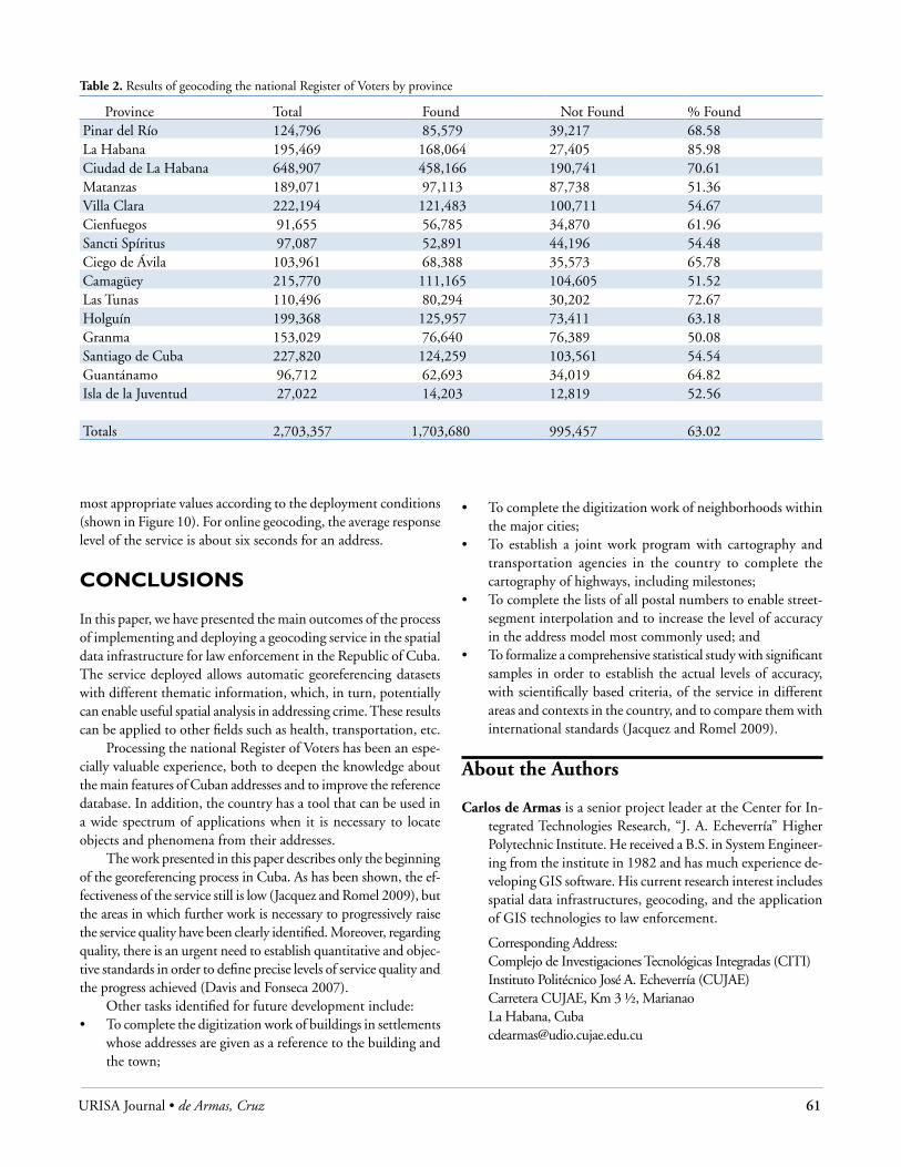
URISA Journal • de Armas, Cruz 61
most appropriate values according to the deployment conditions (shown in Figure 10). For online geocoding, the average response level of the service is about six seconds for an address.
concluSIonS
In this paper, we have presented the main outcomes of the process of implementing and deploying a geocoding service in the spatial data infrastructure for law enforcement in the Republic of Cuba. The service deployed allows automatic georeferencing datasets with different thematic information, which, in turn, potentially can enable useful spatial analysis in addressing crime. These results can be applied to other fields such as health, transportation, etc.
Processing the national Register of Voters has been an espe-cially valuable experience, both to deepen the knowledge about the main features of Cuban addresses and to improve the reference database. In addition, the country has a tool that can be used in a wide spectrum of applications when it is necessary to locate objects and phenomena from their addresses.
The work presented in this paper describes only the beginning of the georeferencing process in Cuba. As has been shown, the ef-fectiveness of the service still is low (Jacquez and Romel 2009), but the areas in which further work is necessary to progressively raise the service quality have been clearly identified. Moreover, regarding quality, there is an urgent need to establish quantitative and objec-tive standards in order to define precise levels of service quality and the progress achieved (Davis and Fonseca 2007).
Other tasks identified for future development include:• To complete the digitization work of buildings in settlements
whose addresses are given as a reference to the building and the town;
• To complete the digitization work of neighborhoods within the major cities;
• To establish a joint work program with cartography and transportation agencies in the country to complete the cartography of highways, including milestones;
• To complete the lists of all postal numbers to enable street-segment interpolation and to increase the level of accuracy in the address model most commonly used; and
• To formalize a comprehensive statistical study with significant samples in order to establish the actual levels of accuracy, with scientifically based criteria, of the service in different areas and contexts in the country, and to compare them with international standards (Jacquez and Romel 2009).
About the Authors
Carlos de Armas is a senior project leader at the Center for In-tegrated Technologies Research, “J. A. Echeverría” Higher Polytechnic Institute. He received a B.S. in System Engineer-ing from the institute in 1982 and has much experience de-veloping GIS software. His current research interest includes spatial data infrastructures, geocoding, and the application of GIS technologies to law enforcement.
Corresponding Address: Complejo de Investigaciones Tecnológicas Integradas (CITI) Instituto Politécnico José A. Echeverría (CUJAE) Carretera CUJAE, Km 3 ½, Marianao La Habana, Cuba [email protected]
Table 2. Results of geocoding the national Register of Voters by province
Province Total Found Not Found % FoundPinar del Río 124,796 85,579 39,217 68.58La Habana 195,469 168,064 27,405 85.98Ciudad de La Habana 648,907 458,166 190,741 70.61Matanzas 189,071 97,113 87,738 51.36Villa Clara 222,194 121,483 100,711 54.67Cienfuegos 91,655 56,785 34,870 61.96Sancti Spíritus 97,087 52,891 44,196 54.48Ciego de Ávila 103,961 68,388 35,573 65.78Camagüey 215,770 111,165 104,605 51.52Las Tunas 110,496 80,294 30,202 72.67Holguín 199,368 125,957 73,411 63.18Granma 153,029 76,640 76,389 50.08Santiago de Cuba 227,820 124,259 103,561 54.54Guantánamo 96,712 62,693 34,019 64.82Isla de la Juventud 27,022 14,203 12,819 52.56
Totals 2,703,357 1,703,680 995,457 63.02

62 URISA Journal • Vol. 25, No. 1 • 2013
Andrei Cruz is an M.S. student at the Computer Science Faculty of Havana University. He has been working with the GIS project at the Center for Integrated Technologies Research, “J. A. Echeverría” Higher Polytechnic Institute. His current research interest is geocoding algorithms.
Corresponding Address: Complejo de Investigaciones Tecnológicas Integradas (CITI) Instituto Politécnico José A. Echeverría (CUJAE) Carretera CUJAE, Km 3 ½, Marianao La Habana, Cuba [email protected]
References
Crossier, S. 2004. ArcGIS 9. Geocoding in ArcGIS. Redlands: Enviromental Systems Research Institute.
Davis, C. A., and F. T. Fonseca. 2007. Assessing the certainty of locations produced by an address geocoding system. Geon-formatica 11: 103-29.
Enviromental Systems Research Institute (ESRI). 2009. ArcGIS 9.3 Geocoding technology. Redlands: ESRI.
Enviromental Systems Research Institute (ESRI). 2010. ArcGIS Desktop 9.3 help. Commonly used address locator styles. Redlands: ESRI.
Gilmore, W. J. 2006. Introducing Google geocoding service. The network for technology professionals. Http://www.developer.com/tech/article.php/3615681/introducing-google-geo coding-service.htm.
Gilmore, W. J. 2006. Performing HTTP geocoding with the Google Maps API. The network for technology profession-als. Http://www.developer.com/db/article.php/3621981/Performing-HTTP-Geocoding-with-the-Google-Maps-API.htm.
Goldberg, D. W., J. P. Wilson, and C. A. Knoblock. 2007. From text to geographic coordinates: The current state of geocod-ing. Journal of the Urban and Regional Information Systems Association 19 (1): 33-46.
Jacquez, G. M., and R. Romel. 2009. Local indicators of geocod-ing accuracy (LIGA): Theory and application. International Journal of Health Geographics 8 (1): 60.
Kothuri, R., A. Godfrind, and E. Beinat. 2007. Pro Oracle spatial for Oracle database 11g. New York: Apress.
Murray, C. 2008. Oracle 11g spatial developer guide. Redwood: Oracle Press.
Shea, C. 2007. Oracle 11g text reference. Redwood: Oracle Press.Swift, J. N., D. W. Goldberg, and J. P. Wilson. 2008. Geocoding
best practices: Review of eight commonly used geocoding systems. Technical Report No. 10, GIS Research Laboratory, University of Southern California, Los Angeles.
Tang, A., and K. Clark. 2003. ArcGIS 9. Geocoding rule base developer guide. Redlands: ESRI.
URISA Journal • Rybarczyk, Mohapatra 63
IntroductIon
In 1949, the U.S. government housing policy formally recognized that residential environment is one crucial element of increasing the quality of life (Dahmann 1985). Since then, many cities throughout the United States have experienced substantial emi-gration, economic decline, poverty, segregation, decentralization, and general strife that counters this housing policy (Kitchen and Williams 2009). Many of these externalities are concentrated in collapsed neighborhoods and communities, vastly decreasing the quality of life for residents within them. To reverse this trend, many U.S. cities are taking appropriate courses of action, starting from understanding the causes to finding solutions that could reverse these effects. Neighborhood planning efforts are often at the forefront of this effort. A notable example can be witnessed in cities that have adopted neotraditional design elements. This plan-ning strategy is formalized under the charter for New Urbanism and posits that proper urban design can create communities that are walkable, bikeable, diverse, dense, and safe, while deterring suburban sprawl and curing ailing communities (Leccese 2000, Day 2003). This strategy has become so popular that the U.S. government views it as a means to alleviate distressed neighbor-hood conditions (Bohl 2000). While this tactic appears promising, defining neighborhoods remains controversial.
The challenge of defining neighborhoods dates back to the 1960s when geographic places were vaguely summarized as conglomerations of commonly held residential attributes (Galster 2001). An example of early neighborhood definition is that of Keller (1968) who posited that neighborhoods consist of
physical as well as symbolic boundaries. Several additional early neighborhood definitions attempted to address intangible views such as commonsense walking limits (Morris and Hess 1975), sociological and ecological paradigms (Schoenberg 1979, Hallman 1984), and spatial boundaries bounded by shared public space or social networks (Schoenberg 1979). Moreover, neighborhood boundary determination, selection of controversial neighborhood attributes, and inefficient modeling strategies remain the norm in many neighborhood studies (Ellen and Turner 1997).
Greenberg (1999) and Galster (2001) suggested that most neighborhood studies do not incorporate the full spectrum of variables that make up neighborhoods, thus compromising the validity of any result. Therefore, in this study, an attempt is put forth to objectively assess neighborhood quality using contextual variables that address three neighborhood factions: sociodemo-graphic, economic, and transportation conditions. The goal of this research is to progress current objective neighborhood analyses by employing easily obtainable variables from administrative sources that will address previous shortcomings regarding neighborhood quality-measurement techniques. The remainder of this paper is organized as follows. The second section presents how neighbor-hoods are defined and assessed, followed by a thorough review of past neighborhood studies that support this research in the next section. The fourth part describes the conceptual framework of this research followed by the study area and the data used in this research. A detailed assessment of the methods utilized is high-lighted in the fifth section. The next part describes the results from the empirical analysis, which is followed by a conclusion.
evaluating neighborhoods through empirical analysis and Geographic Information Systems
Greg Rybarczyk and Rama Prasada Mohapatra
Abstract: Assessing and mapping neighborhood quality has a long legacy toward enhancing the vitality and quality of life in cities in the United States. This study utilized factor analysis and GIS-weighted overlay techniques for assessing neighborhood quality in Milwaukee, Wisconsin. The study integrates several objective neighborhood parameters that address important neighborhood tenets. First, a data-reduction tool was invoked to reduce a large number of variables into several comprehensive indicators that relate to established socioeconomic and contextual paradigms. These factors then were ranked and aggregated using GIS overlay techniques to produce a map depicting neighborhood integrity. The approach shown here demonstrates how several types of administrative datasets can easily be utilized in a GIS-based modeling environment to reach neighborhood quality indices. The results show promise for persons involved in neighborhood planning or defining neighborhoods where objectivity and often multiple competing criteria are present.
PaPerS of PractIce, technIcal rePortS and InduStry noteS
64 URISA Journal • Vol. 25, No. 1 • 2013
defInInG neIGhBorhoodS
The geography of localized social spaces has been studied since at least the early 20th century (Burgess and Park 1925, Shevky and Bell 1955). Neighborhood scale analysis has a rich tradition of representing and deciphering localized forces that affect and shape people’s lives (Galster 2001, Lewicka 2010). The forces that shape and define neighborhoods are deeply rooted in inhabit-ant perception and environmental features that help fortify a fundamental human attachment to a particular space (Jordan et al. 1998, Meersman 2005, Lewicka 2010). Despite the recogniz-able correlation between neighborhoods and the quality of life, defining and operationalizing what constitutes a neighborhood wanes among several disciplines (Galster 2001, Kitchen and Williams 2009).
Neighborhood attributes contain contextual and perceptual properties that typically consist of administrative data sources and intangible societal properties related to social cohesiveness (Sawicki and Flynn 1996, Meersman 2005). Crime, demograph-ics, urban form, transportation, resident personalities, and land uses are some of the typical factors used in neighborhood analysis (Greenberg 1999, Sampson 2003). Many of these variables can be found in neighborhood studies related to planning (Huxhold 1996), health (Krieger 2003), brownfields (Clarke 1997), urban-change analysis (Kitchen and Williams 2009), child development (Ellen and Turner 1997), crime (Murray et al. 2001), and sustain-able transportation (Black et al. 2002). A notable neighborhood assessment is the National Neighborhood Indicators Project (Sawicki and Flynn 1996). This multiyear project advanced the institutionalization of neighborhood measures for changing social, physical, and economic conditions in the United States.
The commonality among all neighborhood studies is the importance of human perception and environmental objects. This dynamic link has been substantiated by Meersman (2005), who postulated that neighborhood properties may serve as pre-cursors to perceptions of neighborhoods. In addition, Meersman (2005) also found correlations between observable variables of neighborhood quality and subjective responses to neighborhood conditions. Perception of space as afforded by the environment can be linked to Gibson’s (1979) theory of ecological psychology. This theory posits that humans inherently view space in optic arrays and subsequent affordances. The objects present in one’s view then impact information received by them, thus affecting how they define and interact within this space. This finding also is observed in the work of Hillier (1996), who claimed that environmental design and space dictates human interaction and social organization. We can infer from this that environmental objects are integral in neighborhood perception.
neIGhBorhood MeaSureMent StrateGIeS
Neighborhoods can be assessed either subjectively or objectively, or in combination. For example, Hoehner et al. (2005) utilized perceptual and objective neighborhood attributes to determine their influence on a respondent’s physical activity. Subjective measures require the collection of responses from persons to measure perceptions and attitudes of the immediate environ-ment. Qualitative data can include resident responses of neigh-borhood safety, disorder, and social interactions (Raudenbush 1999, Krieger 2003). Conversely, objective measures utilize data typically derived from administrative sources where neighbor-hood attributes are represented without inclusion of perceptual insights. Quantitative data generally are obtained from the U.S. Census, police departments, departments of natural resources, other government departments, public health surveys, etc. Ob-jective data have been used to measure pedestrian accessibility within neighborhoods (Aultman-Hall et al. 1997), personal health and neighborhoods (Diez-Roux 2001), and food environments (Cummins 2006), to name a few. In many studies, objective and subjective datasets are used together because of the complicated nature of what constitutes a neighborhood.
Objective neighborhood attributes and subjective neigh-borhood perceptions have been found to be congruent in many studies. This finding was highlighted by Quillian and Page (2001), where it was discovered that racial composition of the survey par-ticipants was correlated to perceptions of crime levels, but when objectively determined crime rates proved otherwise. Similarly, Sampson and Raudenbush (2004) found that the socioeconomic status and ethnicity of neighborhoods predicted the perception of crime and disorder when objective measures were controlled. Jacob (1994) found incongruent statistical results between Penn-sylvania residents choices and county government data. This also is corroborated by studies that have determined that neighborhood residents, when asked about their neighborhoods, can neither provide unbiased assessments nor agree on what neighborhood attributes matter most (Ellen and Turner 1997). Despite the vast array of qualitative and quantitative information available and apparent alignment between empirical and perceptual neighbor-hood outputs, efficient model development and the selection of suitable data types remain a significant research agenda in many neighborhood analyses.
A strategy that often is used to assess subjective and objec-tive neighborhood data involves the integration of geographic information systems (GIS). GIS has the unique ability to man-age, visualize, and analyze data, and has been used extensively in land use, zoning, transportation, urban modeling, neighborhood planning, participatory planning, and economic development (Huxhold 1996, Sui 1998, Peng 2001, Ghose and Huxhold 2002, Fotheringham 2004). GIS’s greatest asset is the capacity to spa-tially analyze multiple datasets and layers and, subsequently, view the interactions between them. This benefit allows stakeholders

URISA Journal • Rybarczyk, Mohapatra 65
to spatially view the complex connections between person and place—which is vital to neighborhood studies (Sawicki and Flynn 1996). GIS methods have made great strides toward objectively as-sessing and visualizing neighborhood planning (Sawicki and Flynn 1996, Kellogg 1999, Ghose and Huxhold 2002, Talen 2005, 2007). For instance, Ghose et al. (2002) utilized GIS extensively as a visualization and mapping tool to quantify neighborhood health at varying geographic scales. Furthermore, neighborhood indicators and GIS methods have garnered much attention be-cause they are seen as a legitimate and objective multiscale tool that can have a large impact on individuals (Ghose and Huxhold 2002). GIS also has been employed in developing neighborhood quality indices. Index development represents a condensed fac-tor derived from a large number of other influential variables (Ebert and Welsch 2004). The influential variables then can be represented as “layers” in a GIS. In neighborhood analysis, the layers can be weighted based on importance. A weighting method requires that the weights be assigned by expert knowledge or by statistical derivations. The expert knowledge method weighs layers based on the perceptions of the researcher or of a group of professionals (experts) (Hagerty and Land 2002). A common statistical weighting method is the simple additive approach, where the attribute data is summed after multiplying the weights with the indicators to derive a composite output (Malczewski 2005). For example, Talen (2005) utilized multiple GIS layers and overlaid them using a similar type of weighting scheme to produce a composite map of desirable neighborhood urban form.
Index development typically involves a multitude of factors and often is difficult to assess because of highly correlated response variables. Data-reduction techniques such as factor analysis are suitable to neighborhood analysis because factor analysis can depict spatial patterns between numerous quantities and facets of neighborhood quality. The utility of this method is that it can quickly assess and reveal underlying relationships among many, often diverse, variables (O’Sullivan and Unwin 2003). For ex-ample, Johnston et al. (2004) utilized factor analysis to determine homogenous response variables to predict how neighborhood context affected voter turnout at multiple scales. Also a study by Doolittle et al. (1978) in Milwaukee, Wisconsin, used fac-tor analysis to group “sense of community” indicators and then verified them with local community members. Another notable study conducted by Ross et al. (1999) used factor analysis to aggregate many objective contextual factors to measure neigh-borhood disorder.
concePtual fraMeworK
Clearly, for neighborhood quality assessment, myriad contextual data that can be analyzed using empirical methodologies are the need of the hour. Furthermore, there is a need to integrate a robust data-reduction technique such as factor analysis and GIS so that the quality of the neighborhoods can be portrayed in the form of a simple map. The framework for this study is based on the integra-tion of economic, sociodemographic, and transportation assets of
neighborhoods to measure neighborhood quality (see Figure 1). While previous literature has determined that sociodemographic and economic conditions contribute to neighborhood quality, less research exists regarding how transportation features contribute to this effect. This research expands on current neighborhood analysis by specifically including objective transportation variables pertaining to neighborhood quality. The impetus for addressing transportation conditions within neighborhoods stems largely from the public health and planning fields. A growing number of studies in these areas have directly linked the influence the built environment holds in facilitating active modes of transportation (Saelens et al. 2003). Neighborhoods that contain transportation diversity, such as bicycling and walking facilities, may increase residential mobility and access, increase residents’ personal health (Saelens et al. 2003, Weden 2008), deter crime (Newman and Kenworthy 1999), and increase social efficacy (Saelens et al. 2003). In terms of neighborhood quality, Greenberg (1999) discovered that the lack of mass-transit options coupled with apparent blight contributed to low neighborhood quality. As an extension of this work, Cervero (2003) posited that walkable neighborhoods often are self-selected by residents, validating the notion that neighborhood quality is influenced by its transporta-tion options. The role of transportation infrastructure, especially those that encourage active modes of transportation, cannot be understated while assessing neighborhood quality. Therefore, this research operationalizes several transportation, economic, and sociodemographic conditions to determine a reliable mea-sure of neighborhood quality using GIS-based weighted overlay techniques and weights derived through factor analysis. The relationship between the three neighborhood components and the considered variables that fall within are displayed in Figure 1.
data and Study area
Milwaukee neighborhoods have strong ties to the community, but, like many major cities in the United States, they are not without problems such as poverty, blight, segregation, and so-cioeconomic disparities (Ghose and Huxhold 2002). To counter these problems, the city of Milwaukee and the Community Block Grant Administration (CBGA) have made concerted efforts to distribute federal monies to neighborhoods with need (Ghose
Figure 1. Relationship between neighborhood components

66 URISA Journal • Vol. 25, No. 1 • 2013
income, race, gender, and household size were obtained for the 2000 U.S. Census Bureau at the block level. The 2006 Milwaukee Master Property File (MPROP) data were obtained from the City of Milwaukee Information Technology Management Department. The information used from this dataset includes the current and the past year’s property and building values, as determined by the city assessor’s office, as well as the number of building rooms, total number of rooms, bathrooms, building height, parcel size, and land use. These factors provide insight into the general housing condition and quality, housing density, and land-use diversity. Parks, schools, and recreational area data were obtained from the Milwaukee County Parks Department and were utilized in this study to account for desirable neighborhood attractions and the density of public space per neighborhood. Public spaces such as these represent areas for people to congregate and promote chance encounters that serve to strengthen community bonds (Langdon 1997). Business data consisting of gasoline/convenience stores were obtained from the city of Milwaukee and selected via the federal Standard Industrial Classification code. These data attend to explicit ingredients needed to produce viable heterogeneous neighborhoods (Talen 1999). The presence of noxious land uses has been shown to correlate to neighborhood disinvestment and disorder (Greenberg et al. 2000). As a result, the toxic-release inventory dataset was obtained from the Wisconsin Department of Natural Resources (WIDNR). Crime at any level is associated with neighborhood disorder (Dahmann 1985, Ross and Mirowsky 1999). Therefore, all crimes from the year 2000 were obtained from the Milwaukee Police Department via the MV400 database and included in this study.
The GIS road network layer used in this research consists of the Fire Dual Independent Map Encoding (DIME) developed by the city of Milwaukee and is currently the most precise road net-work available. Highway engineering road variables for all roads in southeastern Wisconsin were obtained from the Wisconsin Department of Transportation (WIDOT). The engineering road
Table 1. Variables and data sources
Name of the Variables Description
White Total proportional white population (percent)
Black Total proportional African-American population (percent)
Male Male population (percent)
Female Female population (percent)
Pop < 5 Population (percent) in the age group under 5
Pop 5-17 Population (percent) in the age group 5 to 17
Pop 18-22 Population (percentage) in the age group 18 to 22
Pop 22-30 Population (percent) in the age group 22 to 30
Pop 30-40 Population (percent) in the age group 30 to 40
Pop 40-49 Population (percent) in the age group 40 to 49
Pop 50-65 Population (percent) in the age group 50 to 65
Pop >65 Population (percent) greater than 65
Median Age Male Average of median age of males
Median Age Female Average of median age of females
Family Size Average of family size
Current Land Value Average of the current land assessed value
Current Improvement Value The average of the current assessed value of all improvements on the property
Current Total Value The average of the sum of current assessed land and improvement value
Previous Land Value The average of the previous year’s assessed land value
Previous Improvement Value The average of the previous year’s assessed property improvement value
Previous Total Value The average of the sum of the previous year’s assessed land and improvement value
Households Total number of households
Household Size Average of household size
Owner Occupied Total number of owner-occupied dwellings
Renter Occupied Total number of renter-occupied dwellings
Number of StoriesThe average of the number of stories above grade in the building (does not include the basement). For multistructure properties, the number of stories of the predominant build-ing is shown.
Housing Units Summation of the number of dwelling units on the property
Building Area Average of the total usable floor area of the structure in square feet
Number of RoomsAverage of the total number of rooms per total dwelling units (total room count excluding bathrooms, powder rooms, and recreation rooms; this total includes sunrooms, breezeways, and legal basement bedrooms)
Bedrooms Average of number of bedrooms per dwelling unit
BathroomsAverage of total number of bathrooms per dwelling unit (total number of bathrooms in the building or the number of bathrooms predominantly found in each dwelling unit)
Lot Area Average size of the property in square feet
Median Household Income Average of median household income
Land-use TypesCount of different types of land uses (land use code 5000 to 6000 from MPROP data was used to get the number)
Toxic -release Sites Summation of the total number of toxic releases per neighborhood
Number of Crimes Summation of the total number of all crimes per neighborhood
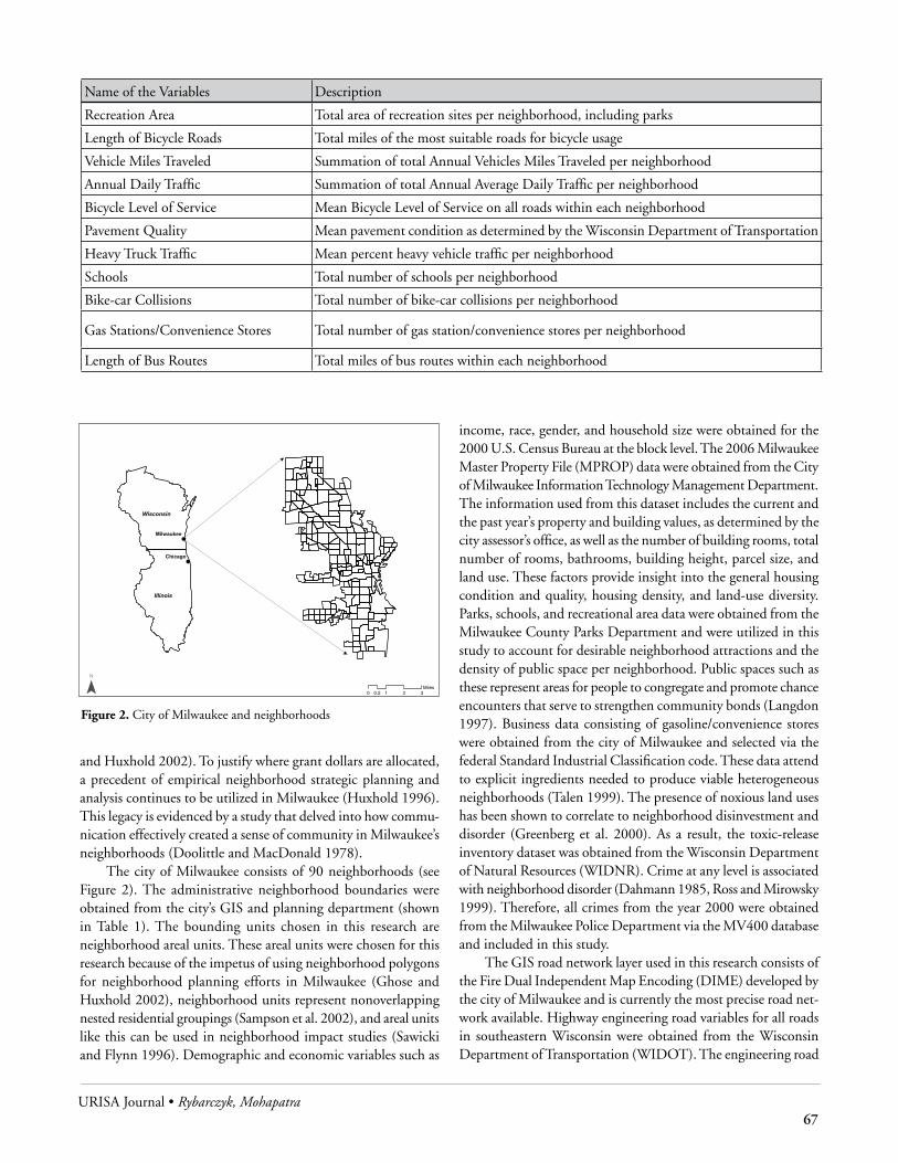
URISA Journal • Rybarczyk, Mohapatra 67
and Huxhold 2002). To justify where grant dollars are allocated, a precedent of empirical neighborhood strategic planning and analysis continues to be utilized in Milwaukee (Huxhold 1996). This legacy is evidenced by a study that delved into how commu-nication effectively created a sense of community in Milwaukee’s neighborhoods (Doolittle and MacDonald 1978).
The city of Milwaukee consists of 90 neighborhoods (see Figure 2). The administrative neighborhood boundaries were obtained from the city’s GIS and planning department (shown in Table 1). The bounding units chosen in this research are neighborhood areal units. These areal units were chosen for this research because of the impetus of using neighborhood polygons for neighborhood planning efforts in Milwaukee (Ghose and Huxhold 2002), neighborhood units represent nonoverlapping nested residential groupings (Sampson et al. 2002), and areal units like this can be used in neighborhood impact studies (Sawicki and Flynn 1996). Demographic and economic variables such as
income, race, gender, and household size were obtained for the 2000 U.S. Census Bureau at the block level. The 2006 Milwaukee Master Property File (MPROP) data were obtained from the City of Milwaukee Information Technology Management Department. The information used from this dataset includes the current and the past year’s property and building values, as determined by the city assessor’s office, as well as the number of building rooms, total number of rooms, bathrooms, building height, parcel size, and land use. These factors provide insight into the general housing condition and quality, housing density, and land-use diversity. Parks, schools, and recreational area data were obtained from the Milwaukee County Parks Department and were utilized in this study to account for desirable neighborhood attractions and the density of public space per neighborhood. Public spaces such as these represent areas for people to congregate and promote chance encounters that serve to strengthen community bonds (Langdon 1997). Business data consisting of gasoline/convenience stores were obtained from the city of Milwaukee and selected via the federal Standard Industrial Classification code. These data attend to explicit ingredients needed to produce viable heterogeneous neighborhoods (Talen 1999). The presence of noxious land uses has been shown to correlate to neighborhood disinvestment and disorder (Greenberg et al. 2000). As a result, the toxic-release inventory dataset was obtained from the Wisconsin Department of Natural Resources (WIDNR). Crime at any level is associated with neighborhood disorder (Dahmann 1985, Ross and Mirowsky 1999). Therefore, all crimes from the year 2000 were obtained from the Milwaukee Police Department via the MV400 database and included in this study.
The GIS road network layer used in this research consists of the Fire Dual Independent Map Encoding (DIME) developed by the city of Milwaukee and is currently the most precise road net-work available. Highway engineering road variables for all roads in southeastern Wisconsin were obtained from the Wisconsin Department of Transportation (WIDOT). The engineering road
Figure 2. City of Milwaukee and neighborhoods
Name of the Variables Description
Recreation Area Total area of recreation sites per neighborhood, including parks
Length of Bicycle Roads Total miles of the most suitable roads for bicycle usage
Vehicle Miles Traveled Summation of total Annual Vehicles Miles Traveled per neighborhood
Annual Daily Traffic Summation of total Annual Average Daily Traffic per neighborhood
Bicycle Level of Service Mean Bicycle Level of Service on all roads within each neighborhood
Pavement Quality Mean pavement condition as determined by the Wisconsin Department of Transportation
Heavy Truck Traffic Mean percent heavy vehicle traffic per neighborhood
Schools Total number of schools per neighborhood
Bike-car Collisions Total number of bike-car collisions per neighborhood
Gas Stations/Convenience Stores Total number of gas station/convenience stores per neighborhood
Length of Bus Routes Total miles of bus routes within each neighborhood
!
!
Illinois
Wisconsin
Chicago
Milwaukee
¯ 0 1 2 30.5Miles

68 URISA Journal • Vol. 25, No. 1 • 2013
data, coupled with the Fire DIME network, contain traffic counts, heavy truck volume, and travel lanes. These variables will provide additional insight regarding the intensity of traffic and design in each neighborhood. The use of nonmotorized transportation is primarily used by poverty-stricken populations and also serves as an indicator of neighborhood attractiveness (Gannon and Liu 1997, Saelens et al. 2003). Currently, 96.5 miles of on-street bicycle facilities exist in the city of Milwaukee and more than 100 miles of off-street bicycle routes (Turner 1997). Bicycle ac-cident vector point data from the year 2003 was obtained from the Milwaukee Police Department. The bicycle crash data was added to serve as an indicator of traffic-bicycle safety conditions in each neighborhood. A Bicycle Level of Service (BLOS) safety index also was included in this study. The algorithm consists of per-lane motor vehicle traffic volume, speed of motor vehicles, traffic mix, potential cross-street traffic generation, pavement surface condition, and pavement width for bicycling various roadway infrastructures, such as average daily traffic, roadway width, traffic speeds (Landis et al. 1997).
MethodoloGy:analySIS of MIlwauKee’S neIGhBorhoodS
After the pertinent data was obtained, it was aggregated or extrapolated based on the existing neighborhood boundaries of Milwaukee. Although various datasets used in this analysis originated from differing scales and differing geographic units, maximum attention was given while aggregating or extrapolating the data to minimize the modifiable areal unit problem (MAUP). The purpose of aggregating various neighborhood attributes in this study is to examine latent phenomena within neighborhoods to derive an empirical index. In addition, no statistical relation-ships are pursued in this research where spurious correlations or regression results would ensue based on the MAUP. Furthermore, one instance where the MAUP is not a factor is when “true ag-gregation” is utilized to uncover a phenomenon that is related to the combination of the areal constituents (Tobler 1989).
In this research, initially, exploratory data analysis was carried out to better understand the relationship within and among dif-
ferent variables. To reduce the dimensionality of the data, factor analysis was carried out in the SPSS statistical software (SPSS Inc. Chicago, IL). Factor analysis has the distinct advantage of reduc-ing the initial number of variables into lesser number of variables called “factors” with a minimal loss of information (Hair, Jr., et al. 1995). The fundamental assumption of factor analysis is that few underlying factors that are lesser in number than the number of observed variables are responsible for the covariation among the observed variables (Kim 1978a). In this research, we have used exploratory factor analysis, which used the principal component method to extract the factors, and then applied a Varimax rota-tion with Kaiser Normalization to retain only those factors whose eigenvalues exceeded 1.0. The exploratory factor analysis produces a scree plot, a simple line-segment plot that shows the number of factors against their corresponding eigenvalues, which can be used to extract the appropriate number of factors (Kim 1978b). Factor analysis also produces factor loadings and factor scores. Factor loadings explain the relationship between individual initial variables and a particular factor. A factor loading value close to ± 1.0 indicates a strong relationship between the variable and the factor. Also, apart from being helpful in reducing the dimen-sionality of data, factor analysis is helpful in determining the underlying structure of neighborhood indicators and could form groups of like indicators as homogenous groups or factors (Ross and Mirowsky 1999). Factor scores are standardized values for each and every neighborhood where a higher score means that the factor under consideration has a strong influence on that particular neighborhood. Furthermore, the factor analysis also yields the percentage variance of each and every factor that can be used as weight to differentiate cases (in our case, neighborhoods). If we go for equal weighting of factors, then those factors accounting for considerable variance and those accounting for little would be given equal importance. However, a solution can be to multiply the factor scores with the percentage variance accounted for by the factor (Rummel 1970).
In this study, an indexed map overlay technique was used in a GIS environment that employed factor scores to form a composite index that then enabled the production of a single thematic map that could help evaluate the neighborhoods of Milwaukee. The index overlay technique is a traditional procedure to reduce several metrics into one overall comprehensive index (O’Sullivan and Unwin 2003). In this study, the factor scores were combined in
Table 2. Factor score classes and ranks
Factor 1 Factor 2 Factor 3 Factor 4 Factor 5 Factor 6 Factor 7 Factor 8 Factor 9 Factor 10Class 1 1 7 7 1 1 1 1 1 1 1Class 2 2 6 6 2 2 2 2 2 2 2Class 3 3 5 5 3 3 3 3 3 3 3Class 4 4 4 4 4 4 4 4 4 4 4Class 5 5 3 3 5 5 5 5 5 5 5Class 6 6 2 2 6 6 6 6 6 6 6Class 7 7 1 1 7 7 7 7 7 7 7
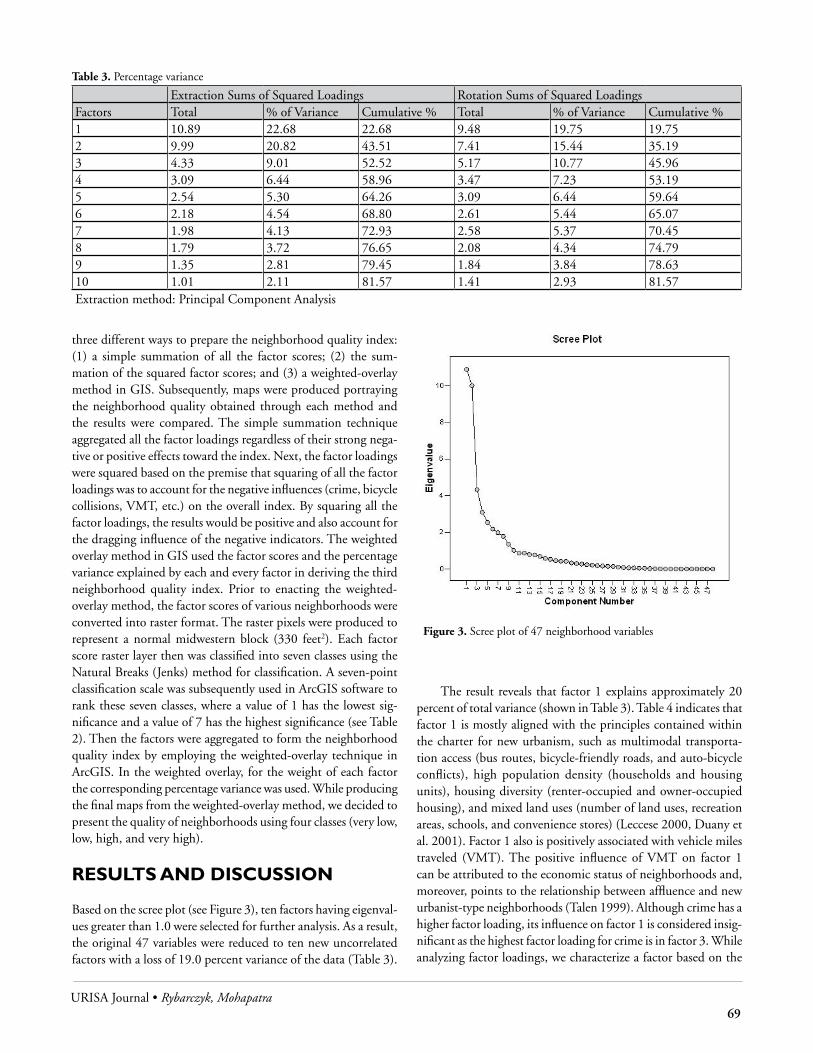
URISA Journal • Rybarczyk, Mohapatra 69
three different ways to prepare the neighborhood quality index: (1) a simple summation of all the factor scores; (2) the sum-mation of the squared factor scores; and (3) a weighted-overlay method in GIS. Subsequently, maps were produced portraying the neighborhood quality obtained through each method and the results were compared. The simple summation technique aggregated all the factor loadings regardless of their strong nega-tive or positive effects toward the index. Next, the factor loadings were squared based on the premise that squaring of all the factor loadings was to account for the negative influences (crime, bicycle collisions, VMT, etc.) on the overall index. By squaring all the factor loadings, the results would be positive and also account for the dragging influence of the negative indicators. The weighted overlay method in GIS used the factor scores and the percentage variance explained by each and every factor in deriving the third neighborhood quality index. Prior to enacting the weighted-overlay method, the factor scores of various neighborhoods were converted into raster format. The raster pixels were produced to represent a normal midwestern block (330 feet2). Each factor score raster layer then was classified into seven classes using the Natural Breaks (Jenks) method for classification. A seven-point classification scale was subsequently used in ArcGIS software to rank these seven classes, where a value of 1 has the lowest sig-nificance and a value of 7 has the highest significance (see Table 2). Then the factors were aggregated to form the neighborhood quality index by employing the weighted-overlay technique in ArcGIS. In the weighted overlay, for the weight of each factor the corresponding percentage variance was used. While producing the final maps from the weighted-overlay method, we decided to present the quality of neighborhoods using four classes (very low, low, high, and very high).
reSultS and dIScuSSIon
Based on the scree plot (see Figure 3), ten factors having eigenval-ues greater than 1.0 were selected for further analysis. As a result, the original 47 variables were reduced to ten new uncorrelated factors with a loss of 19.0 percent variance of the data (Table 3).
The result reveals that factor 1 explains approximately 20 percent of total variance (shown in Table 3). Table 4 indicates that factor 1 is mostly aligned with the principles contained within the charter for new urbanism, such as multimodal transporta-tion access (bus routes, bicycle-friendly roads, and auto-bicycle conflicts), high population density (households and housing units), housing diversity (renter-occupied and owner-occupied housing), and mixed land uses (number of land uses, recreation areas, schools, and convenience stores) (Leccese 2000, Duany et al. 2001). Factor 1 also is positively associated with vehicle miles traveled (VMT). The positive influence of VMT on factor 1 can be attributed to the economic status of neighborhoods and, moreover, points to the relationship between affluence and new urbanist-type neighborhoods (Talen 1999). Although crime has a higher factor loading, its influence on factor 1 is considered insig-nificant as the highest factor loading for crime is in factor 3. While analyzing factor loadings, we characterize a factor based on the
Figure 3. Scree plot of 47 neighborhood variables
Table 3. Percentage variance
Extraction Sums of Squared Loadings Rotation Sums of Squared LoadingsFactors Total % of Variance Cumulative % Total % of Variance Cumulative %1 10.89 22.68 22.68 9.48 19.75 19.752 9.99 20.82 43.51 7.41 15.44 35.193 4.33 9.01 52.52 5.17 10.77 45.964 3.09 6.44 58.96 3.47 7.23 53.195 2.54 5.30 64.26 3.09 6.44 59.646 2.18 4.54 68.80 2.61 5.44 65.077 1.98 4.13 72.93 2.58 5.37 70.458 1.79 3.72 76.65 2.08 4.34 74.799 1.35 2.81 79.45 1.84 3.84 78.6310 1.01 2.11 81.57 1.41 2.93 81.57Extraction method: Principal Component Analysis
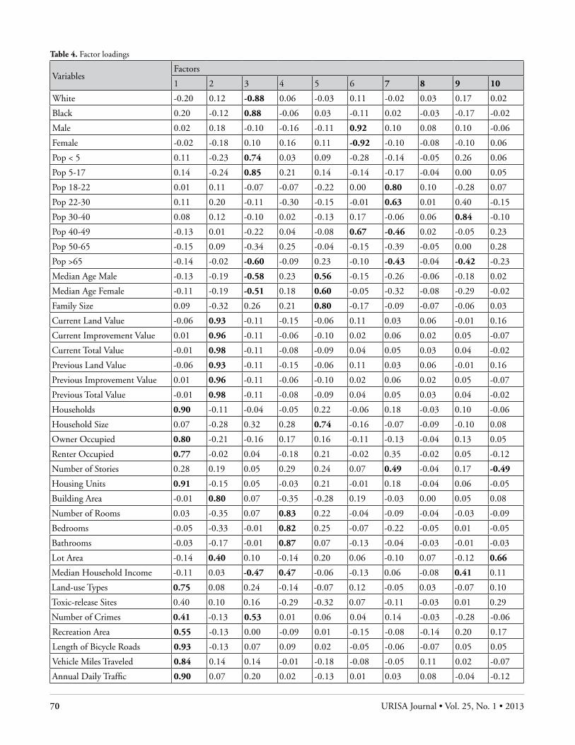
70 URISA Journal • Vol. 25, No. 1 • 2013
Table 4. Factor loadings
VariablesFactors
1 2 3 4 5 6 7 8 9 10
White -0.20 0.12 -0.88 0.06 -0.03 0.11 -0.02 0.03 0.17 0.02
Black 0.20 -0.12 0.88 -0.06 0.03 -0.11 0.02 -0.03 -0.17 -0.02
Male 0.02 0.18 -0.10 -0.16 -0.11 0.92 0.10 0.08 0.10 -0.06
Female -0.02 -0.18 0.10 0.16 0.11 -0.92 -0.10 -0.08 -0.10 0.06
Pop < 5 0.11 -0.23 0.74 0.03 0.09 -0.28 -0.14 -0.05 0.26 0.06
Pop 5-17 0.14 -0.24 0.85 0.21 0.14 -0.14 -0.17 -0.04 0.00 0.05
Pop 18-22 0.01 0.11 -0.07 -0.07 -0.22 0.00 0.80 0.10 -0.28 0.07
Pop 22-30 0.11 0.20 -0.11 -0.30 -0.15 -0.01 0.63 0.01 0.40 -0.15
Pop 30-40 0.08 0.12 -0.10 0.02 -0.13 0.17 -0.06 0.06 0.84 -0.10
Pop 40-49 -0.13 0.01 -0.22 0.04 -0.08 0.67 -0.46 0.02 -0.05 0.23
Pop 50-65 -0.15 0.09 -0.34 0.25 -0.04 -0.15 -0.39 -0.05 0.00 0.28
Pop >65 -0.14 -0.02 -0.60 -0.09 0.23 -0.10 -0.43 -0.04 -0.42 -0.23
Median Age Male -0.13 -0.19 -0.58 0.23 0.56 -0.15 -0.26 -0.06 -0.18 0.02
Median Age Female -0.11 -0.19 -0.51 0.18 0.60 -0.05 -0.32 -0.08 -0.29 -0.02
Family Size 0.09 -0.32 0.26 0.21 0.80 -0.17 -0.09 -0.07 -0.06 0.03
Current Land Value -0.06 0.93 -0.11 -0.15 -0.06 0.11 0.03 0.06 -0.01 0.16
Current Improvement Value 0.01 0.96 -0.11 -0.06 -0.10 0.02 0.06 0.02 0.05 -0.07
Current Total Value -0.01 0.98 -0.11 -0.08 -0.09 0.04 0.05 0.03 0.04 -0.02
Previous Land Value -0.06 0.93 -0.11 -0.15 -0.06 0.11 0.03 0.06 -0.01 0.16
Previous Improvement Value 0.01 0.96 -0.11 -0.06 -0.10 0.02 0.06 0.02 0.05 -0.07
Previous Total Value -0.01 0.98 -0.11 -0.08 -0.09 0.04 0.05 0.03 0.04 -0.02
Households 0.90 -0.11 -0.04 -0.05 0.22 -0.06 0.18 -0.03 0.10 -0.06
Household Size 0.07 -0.28 0.32 0.28 0.74 -0.16 -0.07 -0.09 -0.10 0.08
Owner Occupied 0.80 -0.21 -0.16 0.17 0.16 -0.11 -0.13 -0.04 0.13 0.05
Renter Occupied 0.77 -0.02 0.04 -0.18 0.21 -0.02 0.35 -0.02 0.05 -0.12
Number of Stories 0.28 0.19 0.05 0.29 0.24 0.07 0.49 -0.04 0.17 -0.49
Housing Units 0.91 -0.15 0.05 -0.03 0.21 -0.01 0.18 -0.04 0.06 -0.05
Building Area -0.01 0.80 0.07 -0.35 -0.28 0.19 -0.03 0.00 0.05 0.08
Number of Rooms 0.03 -0.35 0.07 0.83 0.22 -0.04 -0.09 -0.04 -0.03 -0.09
Bedrooms -0.05 -0.33 -0.01 0.82 0.25 -0.07 -0.22 -0.05 0.01 -0.05
Bathrooms -0.03 -0.17 -0.01 0.87 0.07 -0.13 -0.04 -0.03 -0.01 -0.03
Lot Area -0.14 0.40 0.10 -0.14 0.20 0.06 -0.10 0.07 -0.12 0.66
Median Household Income -0.11 0.03 -0.47 0.47 -0.06 -0.13 0.06 -0.08 0.41 0.11
Land-use Types 0.75 0.08 0.24 -0.14 -0.07 0.12 -0.05 0.03 -0.07 0.10
Toxic-release Sites 0.40 0.10 0.16 -0.29 -0.32 0.07 -0.11 -0.03 0.01 0.29
Number of Crimes 0.41 -0.13 0.53 0.01 0.06 0.04 0.14 -0.03 -0.28 -0.06
Recreation Area 0.55 -0.13 0.00 -0.09 0.01 -0.15 -0.08 -0.14 0.20 0.17
Length of Bicycle Roads 0.93 -0.13 0.07 0.09 0.02 -0.05 -0.06 -0.07 0.05 0.05
Vehicle Miles Traveled 0.84 0.14 0.14 -0.01 -0.18 -0.08 -0.05 0.11 0.02 -0.07
Annual Daily Traffic 0.90 0.07 0.20 0.02 -0.13 0.01 0.03 0.08 -0.04 -0.12

URISA Journal • Rybarczyk, Mohapatra 71
highest factor loadings of a variable (Rummel 1970). Moreover, within factor 1, the variables having high factor loadings relate to the characteristics of smart urban growth; thus, we name this factor the “new urbanism” factor.
From the results it was found that the next significant factor (factor 2) relates to land and structure value. Also found was a strong positive linear relation between land value and size. Factor 2 explains approximately 15.5 percentage of total variance (see Table 3). This factor is very important for the quality and price of both the land and building are crucial for good quality sustainable neighborhoods. The results reveal that factor 2 is highly correlated with both the current year’s and previous year’s assessed value of land and building (shown in Table 4). Furthermore, neighbor-hoods having higher factor 2 scores are those with larger lots and high-valued properties. As the study included Milwaukee down-town and the commercial properties within the neighborhoods,
Figure 4. Factor Score Maps, City of Milwaukee, WI
VariablesFactors
1 2 3 4 5 6 7 8 9 10
Bicycle Level of Service -0.01 0.11 -0.01 -0.03 -0.13 0.06 0.09 0.94 -0.02 0.04
Pavement Quality -0.01 0.08 0.08 -0.40 0.01 0.08 -0.10 0.41 -0.10 -0.43
Heavy Truck Traffic -0.03 0.02 -0.06 -0.06 -0.01 0.07 0.02 0.94 0.09 -0.02
Schools 0.69 0.14 0.20 0.01 -0.06 0.08 0.27 -0.06 -0.12 -0.15
Bike-car Collisions 0.72 -0.02 0.37 -0.01 0.11 0.13 0.23 0.01 -0.12 -0.10
Gas Stations/Convenience Stores 0.66 -0.11 0.08 0.02 0.05 0.03 -0.03 -0.04 0.03 0.00
Length of Bus Routes 0.79 0.18 0.13 0.00 -0.41 0.01 -0.05 0.07 -0.08 -0.04
it was observed that the neighborhoods having elevated factor 2 scores (see Figure 4b) are either in and around downtown or in the northwestern suburbs of the commercial business district (CBD) where the acreage of commercial properties are higher. On the other hand, the neighborhoods having lower factor 2 scores are those with average-sized lots, moderate valued structures, and mixed-land use types that relate to the new urbanism ideals. Therefore, based on the result, we can associate lower factor 2 scores with good quality neighborhoods; thus, this factor is named “property value.”
Factor 3 is positively related to young population, children, crime, and African-American population, and negatively related to the median income and white population (see Table 4). Based on these characteristics, factor 3 speaks of crime and poverty tenets that explain approximately 11.0 percentage of the total variance (see Table 3). So we infer that neighborhoods having higher factor
4a 4b 4c 4d 4e
4g 4h 4i 4j

72 URISA Journal • Vol. 25, No. 1 • 2013
3 scores are those with higher young African-American popula-tion, lower income, lesser white population, and higher crime. We name this factor the “sense of safety.” From the results, factor 4 was found to be positively associated with quality and type of buildings in terms of number of stories, total number of rooms, bedrooms, bathrooms, etc. (see Table 4). Factor 4 also is positively correlated with income that is expected, for housing quality is directly related to income; thus, we find a positive association be-tween these two variables. Factor 4 contains a negatively correlated neighborhood health parameter, toxic-release sites. As evidenced in the literature, noxious land uses have a deleterious effect on neighborhood quality; therefore, this result lends credence to our finding. Moreover, factor 4 explains more than 7.0 percentage of the total variance (see Table 3), which is almost half of the “property value” factor (factor 2). Based on the characteristics of this factor, factor 4 is named “income and house quality” factor.
Factor 5, factor 6, and factor 7 are related to various demo-graphic characteristics of the neighborhoods. In particular, factor 5 is positively related to the average family size and household size in a neighborhood. We name this factor “family structure.” Factor 6 is positively related to the age group from 40 to 50 and negatively related to the female population, so we name it “male population aged 40-50” factor. Factor 7 is positively related to the younger population (age 18 to 30) and is negatively related to
the older population (age 40 and above). So we name this factor “population aged 18-30.” Factor 8 is related to Bicycle Level of Service (BLOS), pavement quality, and the percentage of heavy vehicle traffic (see Table 4). This factor provides an indicator of safe latent transportation mobility conditions in each neighbor-hood. Pavement quality and heavy vehicle traffic are included in the BLOS algorithm, resulting in an expected positive correlation. So we name factor 8 “bikeability.” Factor 9 is positively correlated to people in the age group 30 to 40 and negatively correlated with the people age 65 and above (shown in Table 4). We name factor 9 “population aged 30-40.” Interesting enough, factor 10 displays a positive relationship with average lot area and a nega-tive correlation with the number of stories (see Table 4). It only explains 3.0 percentage of the total variance (Table 3). Therefore, we name this factor “lot area.”
After selecting the ten factors discussed previously, individual factor scores for all the neighborhoods in Milwaukee were ob-tained and then visualized (Figure 4a to 4j) in the ArcGIS envi-ronment to relate it to reality. Subsequently, following the three methods (simple summation of all the factor scores, summation of the squared factor scores, and weighted overlay method), we used the factor scores to produce three composite indices and three thematic maps representing the overall quality of neighbor-hoods in Milwaukee. The factor score summation and squared
Figure 6. Neighborhood squared factor score summationFigure 5. Neighborhood factor score summation

URISA Journal • Rybarczyk, Mohapatra 73
MENOMONEERIVERVALLEY
JUNEAUTOWN
¯1 inch = approx. 4 miles
factor score summation maps are displayed in Figures 5 and 6, respectively. These figures reveal that the marginalized and affluent commercial business neighborhoods conflict with the conceptual framework tenets used in this research. For example, the Juneau Town neighborhood (Figure 7) has a very high index value in both the factor score summation and squared factor score summation maps. We can infer from these outputs that the extraordinarily high commercial land values (factor 2) located in this area are the cause of such a result. The Menomonee River Valley neigh-borhood (Figure 7) also scores unexpectedly high neighborhood quality index values through the squared factor score method. This output is largely because of the elevated “family structure” and “population aged 18-30” factor (factors 5 and 7). These examples produced from the two methodologies point to the need for an empirical strategy that does not overemphasize inordinately high or low factor scores, and, more importantly, provides a means to weigh neighborhood quality attributes, i.e., factors, in a more balanced fashion.
Therefore, following the discussed index weighted overlay method, we used the factor scores and respective percentage variance to prepare a third composite index and a thematic map that appropriately portrays the quality of neighborhoods in Mil-waukee. As discussed earlier, for each and every neighborhood, a seven-point classification scale was used to classify the factor scores
of all the factors. Then these classes for all the factors except factor 2 and factor 3 were ranked in a scale of 1 to 7 (Table 2) where 1 has the lowest significance and 7 has the highest significance in the final index. For factor 2 and factor 3, reverse scales were used, where factor 7 has the lowest significance and 1 has the highest significance (Table 2). This was done because the results revealed that neighborhoods having higher factor 2 (“property value”) and factor 3 (“sense of safety”) scores are not the good quality neighborhoods in the city of Milwaukee. The inverse ranking was based on the premise that the very high prices of land and structures, concentration of commercial land-use types, high crime rate, and higher poverty negatively affects neighbor-hood health and counters new urbanism ideals. When the result obtained through the weighted overlay method (Figure 8) was compared to the results of the other two methods, it was found that the weighted overlay method produced a far better neighbor-hood quality map that relates more realistically. More importantly, the result of this research is in line with the findings of previous neighborhood research conducted on Milwaukee. A study by Doolittle et al. (1978) focused on the Jackson Park neighborhood of Milwaukee and described it as stable and containing adequate educational levels, incomes, home ownership, and population mobility. Through our method, we found that the Jackson Park neighborhood is a high-quality neighborhood (Figure 8), which
Figure 7. Juneau and Menominee Valley neighborhoods
Figure 8. Neighborhood factor score weighted overlay

74 URISA Journal • Vol. 25, No. 1 • 2013
is similar to the findings of Doolittle et al. (1978). Furthermore, Ghose et al. (2002) conducted research on the Lindsay Heights neighborhood because of its “low quality of life.” In our neigh-borhood quality map, obtained through the weighted overlay method, this neighborhood received a low-quality rating (Figure 8). Figure 8 also depicts Juneau Town and Menomonee Valley neighborhoods with more logical quality ratings.
concluSIon
Neighborhood planning continues to be the root of many strat-egies for cities that struggle to remain vibrant in today’s global economy. Since the dawn of neighborhood planning efforts, there have been countless methods and data utilized to derive optimal policies, define boundaries, and create strategies to bring positive change into neighborhoods. To better understand the intricacies of localized neighborhood constructs, a two-pronged approach that consists of objective and/or subjective measures remain at the helm of many neighborhood-planning strategies. However, most of the results are constrained because of the lack of a consensual methodology or dataset that captures all relevant personal, social, economic, or environmental constructs pertinent to neighbor-hoods and necessitates further research.
This research has employed current geospatial technologies to objectively visualize neighborhood health in Milwaukee, Wis-consin. The long-standing tradition of neighborhood analysis, minimal amount of neighborhood studies that address transporta-tion features, and controversial assessment techniques instigated this research. The conceptual framework established in this paper facilitated the analysis and included distinctive transportation features that addressed residential health and neighborhood at-tractiveness. The research framework also included traditional sociodemographic and economic variables appropriate for neigh-borhood health assessment.
The strategy utilized in this study focused on a pure empiri-cal analysis using GIS, factor analysis, and overlay techniques to derive several neighborhood indicator maps until a final output was produced. The factor-analysis method was adapted to uncover latent neighborhood properties based on the variables used in this study. In particular, ten factors were extracted from 47 variables that pertained to the conceptual framework followed in this study and resultantly highlighted underlying neighborhood processes, such as new urbanism principles, property value, sense of safety, income and house quality, family structure, male population aged 40 to 50, population aged 18 to 30, bikeability, population aged 30 to 40, and lot area. The indicator weights were derived and summed up in three different ways to form the composite neighborhood quality index. The common ways of aggregating several factors were compared to the weighted-overlay method result where the percentage variances of various factors were used as weights. Unlike most neighborhood studies that have used factor analysis, this research extended the use of this technique by incorporating the factor variances into the weighted overlay process to derive the composite index map. This insightful ap-
proach to weight derivation is pertinent to neighborhood analysis because it groups highly correlated variables into interpretable categories (factors) that speak to neighborhood quality. The final result is a proof in concept because it portrays the neighborhood conditions relatively accurately without obtaining expert knowl-edge and is in line with the findings of previous neighborhood research conducted in Milwaukee. Moreover, the methodology developed in this paper is adaptable to other focus areas because of the substantiated GIS, overlay, and factor-analysis techniques observed from the literature.
This analysis has produced a data-driven neighborhood quality index evaluation method that is encouraging and highly effective in explaining the neighborhood quality in Milwaukee, Wisconsin, in the form of a map. However, limitations to this work should be noted. For example, stakeholder verification was not utilized to verify neighborhood quality. An extension of this research would entail gathering resident, government, and non-profit organization rankings of these neighborhoods to validate or dispel the results displayed here. This information could be obtained through an online GIS system where stakeholder vali-dation could be aggregated into a database for further statistical analysis. In addition, the replication of this method at differing time periods also would substantiate the methodology used here to determine if changes in neighborhood health are captured over time. Regardless, this notion will provide the basis for further in-quiry. In summary, the research presented here was able to institute a conceptual framework that addressed traditional neighborhood components, with the added value of addressing access and mo-bility, and forward an empirical analysis of neighborhoods that may serve policy makers, community organizations, and other stakeholders to better their community.
About the Authors
Greg Rybarczyk is an assistant professor at the University of Michigan–Flint. His research interests are in geographic information systems (GIS), transportation geography, urban planning, spatial analysis, statistical modeling, and remote sensing.
Corresponding Address: Department of Earth and Resource Science University of Michigan–Flint 516D Murchie Science Building Flint, MI 48502 Phone: (810) 762-3355 Fax: (810) 762-3153 [email protected]
URISA Journal • Rybarczyk, Mohapatra 75
Rama Prasada Mohapatra is an assistant professor in the Depart-ment of Geography at Minnesota State University, Mankato.
Rama Prasada Mohapatra, Ph. D. Assistant Professor Department of Geography Armstrong Hall 7 Minnesota State University, Mankato Mankato, MN 56001 Phone: 507-389-6223 (Office) Phone: 507-389-2617(Department) Fax: 507-389-2980
References
Aultman-Hall, L., M. Roorda, and B. W. Baetz. 1997. Using GIS for evaluation of neighborhood pedestrian accessibil-ity. Journal of Urban Planning and Development 123: 10.
Black, J. A., A. Paez, and P. A. Suthanaya. 2002. Sustainable urban transportation: Performance indicators and some analytical approaches. Journal of Urban Planning and Development 128 (4): 184-209.
Bohl, C. C. 2000. New urbanism and the city: Potential appli-cations and implications for distressed inner city neighbor-hoods. Routledge: Taylor and Francis.
Burgess, E. W., and R. Park. 1925. The city: Suggestions for in-vestigations of human behavior in the urban environment. Chicago: University of Chicago Press.
Cervero, R., and M. Duncan. 2003. Walking, bicycling, and urban landscapes: Evidence from the San Francisco Bay area. 93 (9): 1,478-83.
Clarke, K. C. 1997. Getting started with geographic information systems. Upper Saddle River, NJ: Prentice Hall.
Cummins, S., and S. Macintyre. 2006. Food environments and obesity—neighborhood or nation? International Journal of Epidemiology 35: 100-4.
Dahmann, D. C. 1985. Assessments of neighborhood quality in metropolitan America. Urban Affairs Review 20 (4): 511.
Day, K. 2003. New urbanism and the challenges of designing for diversity. Journal of Planning Education and Research 23 (1): 83.
Diez-Roux, A. V. 2001. Investigating neighborhood and area effects on health. American Journal of Public Health 91: 1,783-9.
Doolittle, R. J., and D. MacDonald. 1978. Communication and a sense of community in a metropolitan neighborhood: A factor analytic examination. Communication Quarterly 26 (3): 2-7.
Duany, A., E. Plater-Zyberk, and J. Speck. 2001. Suburban nation: The rise of sprawl and the decline of the American dream. New York: North Point Press.
Ebert, U., and H. Welsch. 2004. Meaningful environmental indices: A social choice approach. Journal of Environmental Economics and Management 47 (2): 270-83.
Ellen, I. G., and M. A. Turner. 1997. Does neighborhood mat-ter? Assessing recent evidence. Housing Policy Debate 8 (4): 833-66.
Fotheringham, A. S., C. Brunsdon, and M. Charlton. 2004. Quantitative geography perspectives on spatial analysis. London: Sage.
Galster, G. 2001. On the nature of neighborhood. Urban Studies 38 (12): 2,111-24.
Gannon, C. A., and Z. Liu. 1997. Poverty and transport. Wash-ington, DC: World Bank.
Ghose, R., and W. Huxhold. 2002. Role of multiscalar GIS-based indicators studies in formulating neighborhood planning policy. Journal of Urban and Regional Information Systems Association 14 (2): 5-17.
Gibson, J. 1979. The ecological approach to visual perception. Boston, MA: Houghton Mifflin Co.
Greenberg, M., K. Lowrie, L. Solitare, and L. Duncan. 2000. Brownfields, toads, and the struggle for neighborhood rede-velopment. Urban Affairs Review 35 (5): 717.
Greenberg, M. R. 1999. Improving neighborhood quality: A hierarchy of needs. Housing Policy Debate 10 (3): 601-24.
Hagerty, M. R., and K. C. Land. 2002. Constructing sum-mary indices of social well-being: A model for the effect of heterogeneous importance weights. American Sociological Association, Chicago, Illinois, August 16 to 19, 1-53.
Hair, Jr., J. F., R. E. Anderson, R. L. Tatham, and W. C. Black. 1995. Multivariate data analysis: With readings. Upper Saddle River, NJ: Prentice-Hall, Inc.
Hallman, H. W. 1984. Neighborhoods: Their place in urban life. Beverly Hills: Sage Publications.
Hillier, B. 1996. Space is the machine: A configurational theory of architecture. Cambridge: Cambridge University Press.
Hoehner, C. M., L. K. Brennan Ramirez, M. B. Elliott, S. L. Handy, and R. C. Brownson. 2005. Perceived and objec-tive environmental measures and physical activity among urban adults. American Journal of Preventive Medicine 28 (2): 105-16.
Huxhold, W., and M. Martin. 1996. GIS guides city’s neighbor-hood funding efforts. GIS World, June: 54-56.
Jacob, S. G., and F. K. Willits. 1994. Objective and subjective indicators of community evaluation: A Pennsylvania assess-ment. Social Indicators Research 32 (2): 161-77.
Johnston, B., K. Jones, S. Burgess, C. Propper, R. Sarker, and A. Bolster. 2004. Scale, factor analyses, and neighborhood effects. Geographical Analysis 36 (4): 350-68.
Jordan, T., M. Raubal, B. Gartrell, and M. Egenhofer. 1998. An affordance-based model of place in GIS. Eighth Interna-tional Symposium on Spatial Data Handling, Vancouver, B.C., 98-109.
Keller, S. I. 1968. The urban neighborhood: A sociological per-spective. New York: Random House.
76 URISA Journal • Vol. 25, No. 1 • 2013
Kellogg, W. 1999. From the field: Observations on using GIS to develop a neighborhood environmental information system for community-based organizations. Journal of Urban and Regional Information Systems Association 11 (1): 15-32.
Kim, J. O., and C. W. Mueller. 1978b. Factor analysis: Statistical methods and practical issues. Beverly Hills: Sage Publications.
Kim, J. O., and C. W. Mueller. 1978a. Introduction to factor analysis: What it is and how to do it. Beverly Hills: Sage Publications.
Kitchen, P., and A. Williams. 2009. Measuring neighborhood social change in Saskatoon, Canada: A geographic analysis. Urban Geography 30 (3): 261-88.
Krieger, N., J. T. Chen, P. D. Waterman, M. J. Soobader, S. V. Subramanian, and R. Carson. 2003. Choosing area-based socioeconomic measures to monitor social inequalities in low birth weight and childhood lead poisoning: The public health disparities geocoding project (U.S). Journal of Epidemiology and Community Health 57 (3): 186-99.
Landis, B. W., V. R. Vattikuti, and M. T. Brannick. 1997. Real-time human perceptions: Toward a bicycle level of service. Transportation Research Record 1578 (1997): 119-26.
Langdon, P. 1997. A better place to live: Reshaping the American suburb. Amherst: University of Massachusetts Press.
Leccese, M., and K. McCormick, Eds. 2000. Charter of the new urbanism. New York: McGraw-Hill.
Lewicka, M. 2010. What makes neighborhood different from home and city? Effects of place scale on place attachment. Journal of Environmental Psychology 30 (1): 35-51.
Malczewski, J. C. R. 2005. Exploring multicriteria decision strategies in GIS with linguistic quantifiers: A case study of residential quality evaluation. Journal of Geographical Systems 7: 249-68.
Meersman, S. C. 2005. Objective neighborhood properties and perceptions of neighborhood problems: Using a geographic information system (GIS) in neighborhood effects and aging research. Ageing International 30 (1): 63-87.
Morris, D. J., and K. Hess. 1975. Neighborhood power: The new localism. Boston: Beacon Press.
Murray, A. T., I. McGuffog, J. S. Western, and P. Mullins. 2001. Exploratory spatial data analysis techniques for examining urban crime implications for evaluating treatment. British Journal of Criminology 41 (2): 309-29.
Newman, P., and J. R. Kenworthy. 1999. Sustainability and cities: Overcoming automobile dependence. Washington, DC: Island Press.
O’Sullivan, D., and D. J. Unwin. 2003. Geographic information analysis. Hobokon, NJ: John Wiley & Sons, Inc.
Peng, Z. R. 2001. Internet GIS for public participation. Environ-ment and Planning B 28 (6): 889-906.
Quillian, L., and D. Pager. 2001. Black neighbors, higher crime? The role of racial stereotypes in evaluations of neighborhood crime. American Journal of Sociology 107 (3): 717-67.
Raudenbush, S. W., and R. J. Sampson. 1999. Econometrics: Toward a science of assessing ecological settings, with appli-cation to the systematic social observation of neighborhoods. Sociological Methodology 29: 1-41.
Ross, C. E., and J. Mirowsky. 1999. Disorder and decay. Urban Affairs Review 34 (3): 412.
Rummel, R. J. 1970. Applied factor analysis. Evanston: North-western University Press.
Saelens, B. E., J. F. Sallis, and L. D. Frank. 2003. Environmental correlates of walking and cycling: Findings from the trans-portation, urban design, and planning literatures. Annals of Behavioral Medicine 25 (2): 80-91.
Sampson, R. J. 2003. The neighborhood context of well-being. Perspectives in Biology and Medicine 46 (3): 53.
Sampson, R. J., J. D. Morenoff, and T. Gannon-Rowley. 2002. Assessing neighborhood effects: Social processes and new di-rections in research. Annual Review of Sociology 28: 443-78.
Sampson, R. J., and S. W. Raudenbush. 2004. Seeing disorder: Neighborhood stigma and the social construction of broken windows. Social Psychology Quarterly 67 (4): 319-42.
Sawicki, D. S., and P. Flynn. 1996. Neighborhood indicators: A review of the literature and an assessment of conceptual and methodological issues. Journal of the American Planning Association 62 (2): 165-83.
Schoenberg, S. P. 1979. Criteria for the evaluation of neighbor-hood viability in working-class and low-income areas in core cities. Social Problems 27 (1): 69-78.
Shevky, E., and W. Bell. 1955. Social area analysis: Theory, illus-trative application, and computational procedures. Stanford, CA: Stanford University Press.
Sui, D. Z. 1998. GIS-based urban modeling: Practices, prob-lems, and prospects. International Journal of Geographical Information Science 12 (7): 651-71.
Talen, E. 2005. Evaluating good urban form in an inner-city neighborhood: An empirical application. Journal of Archi-tectural and Planning Research 22 (3): 204.
Talen, E. 1999. Sense of community and neighborhood form: An assessment of the social doctrine of new urbanism. Urban Studies 36 (8): 1,361.
Talen, E., and S. Swasti. 2007. Neighborhood evaluation using GIS. Environment and Behavior 39 (5): 583-615.
Tobler, W. R. 1989. Frame independent spatial analysis. In Goodchild, M., and S. Gopal, Eds. The accuracy of spatial databases. London: Taylor and Francis.
Turner, S., A. Hottenstein, and G. Shunk. 1997. Bicycle and pedestrian travel demand forecasting: Literature review. College Station: Texas Transportation Institute.
Weden, M. M., R. M. Carpiano, and S. A. Robert. 2008. Sub-jective and objective neighborhood characteristics and adult health. Social Science and Medicine 66: 1,256-70.

URISA’s GIS in Public Health ConferenceMiami, FloridaJune 17-20, 2013
GIS-Pro 2013: URISA’s 51st Annual Conference for GIS ProfessionalsProvidence, Rhode IslandSeptember 16-19, 2013
GIS in Transit ConferenceWashington, DCOctober 16-17, 2013
2013 Locating the Future Conference - GIS & 9-1-1... Location is more than an address.St Louis, MissouriNovember 3-6, 2013
GIS/CAMA Technologies ConferenceJacksonville, FloridaFebruary 24-27, 2014
ww
w.
ur
is
a.
or
gUpcoming
conferences

Your Decisions Affect TheirsGovernment decisions affect more than 300
million Americans a year. With Esri® Technology,
you can connect with your entire constituency.
Esri helps you demonstrate accountability, foster
collaboration, and make the effective decisions
that keep your constituents happy.
Copyright © 2011 Esri. All rights reserved.
Learn more at esri.com/urisanews
G48827_URISA-News_MayJun11.indd 1 6/16/11 9:55 AM