geophysical journal internationalseismo.berkeley.edu/~barbara/reprints/masson-gji2015.pdf · yder...

Geophysical Journal InternationalGeophys. J. Int. (2014) 196, 1580–1599 doi: 10.1093/gji/ggt459Advance Access publication 2013 December 9

GJI

Sei

smol

ogy

On the numerical implementation of time-reversal mirrorsfor tomographic imaging

Yder Masson,1 Paul Cupillard,2 Yann Capdeville3 and Barbara Romanowicz4,1,5

1Institut de Physique du Globe, 1 Rue Jussieu F-75005, Paris, France. E-mail: [email protected] de Lorraine, Laboratoire GeoRessources (UMR 7359), F-54500 Vandoeuvre-les-Nancy, France3LPGN, UFR Sciences et Techniques, Universite de Nantes, F-44322 Nantes Cedex 3, France4College de France, 11, Marcelin Berthelot F-75231 Paris Cedex 05, Paris, France5Berkeley Seismological Laboratory, University of California, Berkeley, CA 94720, USA

Accepted 2013 November 7. Received 2013 November 6; in original form 2013 May 8

S U M M A R YA general approach for constructing numerical equivalents of time-reversal mirrors is intro-duced. These numerical mirrors can be used to regenerate an original wavefield locally withina confined volume of arbitrary shape. Though time-reversal mirrors were originally designedto reproduce a time-reversed version of an original wavefield, the proposed method is inde-pendent of the time direction and can be used to regenerate a wavefield going either forward intime or backward in time. Applications to computational seismology and tomographic imagingof such local wavefield reconstructions are discussed. The key idea of the method is to directlyexpress the source terms constituting the time-reversal mirror by introducing a spatial windowfunction into the wave equation. The method is usable with any numerical method based onthe discrete form of the wave equation, for example, with finite difference (FD) methods andwith finite/spectral elements methods. The obtained mirrors are perfect in the sense that noadditional error is introduced into the reconstructed wavefields apart from rounding errors thatare inherent in floating-point computations. They are fully transparent as they do not interactwith waves that are not part of the original wavefield and are permeable to these. We establisha link between some hybrid methods introduced in seismology, such as wave-injection, andthe proposed time-reversal mirrors. Numerical examples based on FD and spectral elementsmethods in the acoustic, the elastic and the visco-elastic cases are presented. They demonstratethe accuracy of the method and illustrate some possible applications. An alternative imple-mentation of the time-reversal mirrors based on the discretization of the surface integrals inthe representation theorem is also introduced. Though it is out of the scope of the paper, theproposed method also apply to numerical schemes for modelling of other types of waves suchas electro-magnetic waves.

Key words: Numerical solutions; Numerical approximations and analysis; Tomography;Seismic tomography; Computational seismology; Wave propagation.

1 I N T RO D U C T I O N

The development of powerful computer clusters and efficient nu-merical computation methods, such as finite difference (FD), finiteelement (FE) and spectral element (SEM) methods has made it pos-sible to compute seismic wave propagation in a heterogeneous 3-DEarth with unprecedented accuracy (e.g. Moczo et al. 2002; Dumb-ser et al. 2007; Peter et al. 2011; Cupillard et al. 2012). However,the cost of these computations is still problematic in many situa-tions. For example, high-resolution imaging of the subsurface inexploration seismology or global scale Earth tomography require atleast a few thousands of such wave propagation simulations. Hence,

part of the ongoing research effort is dedicated to the developmentof faster modelling methods for computing synthetic seismogramsin a 3-D heterogeneous Earth. Capdeville et al. (2002, 2003) pro-posed to couple SEM simulations with normal modes calculation(C-SEM). Robertsson & Chapman (2000) proposed to limit thewave propagation calculations inside a subregion. Nissen-Meyeret al. (2007) used 2-D simulations to compute 3-D seismograms ina 1-D earth model. Capdeville, Guillot & Marigo (2010), Capdev-ille et al. (2013) and Fichtner et al. (2013) developed upscalingtechniques to account for smaller scale heterogeneity at a reducedcomputational cost. Thanks to some of these developments, andfor the first time, Lekic & Romanowicz (2011) and French et al.

1580 C© The Authors 2013. Published by Oxford University Press on behalf of The Royal Astronomical Society.

at University of C

alifornia, Berkeley on Septem

ber 25, 2015http://gji.oxfordjournals.org/

Dow

nloaded from

http://gji.oxfordjournals.org/

Time-reversal mirrors for tomographic imaging 1581

(2013) developed 3-D global models of the upper mantle usingSEM simulations. At the local and continental scale, full wave-form inversions (e.g. adjoint tomography) that are using a largequantity of wave propagation simulations can be implemented oncurrent generation computers (e.g. Bamberger et al. 1982; Chenet al. 2007; Fichtner et al. 2010; Tape et al. 2009; Rickers et al.2012; Zhu et al. 2012; Rickers et al. 2013). Due to their smallersize, these models offer higher resolution. They provide us withimages of the crust and the upper part of the mantle. In an at-tempt to extend such local full waveform inversions into the deepearth, we developed a numerical equivalent of time-reversal mirrorsthat permits to limit the wave propagation computation to a regionof interest within the earth. This paper details the implementationof the proposed time-reversal mirror and discusses some possibleapplications.

Time-reversal, as introduced by Fink et al. (Fink 1992, 1997; Finket al. 1989; Fink et al. 2001) and more recently applied to geophysi-cal problems (e.g. Larmat et al. 2006; Larmat et al. 2008; Montagneret al. 2012) is a two-step process. First, waves propagating through amedium are recorded with an array of transducers. Then, the recordsare reversed in time and re-emitted by the transducers back into themedium, so that the wave energy is refocused in time and spaceat the position of the source. The refocusing property is due to thereciprocity in space and reversibility in time of the elastic/acousticwave equation, provided that attenuation is negligible. The arrayof transducers used for time reversal is commonly referred to asa time-reversal mirror, or, as a time-reversal cavity, in the specialcase where it forms a closed surface. In theory, it is possible toregenerate the time reversed version of the original wavefield insidea time-reversal cavity by recording the wavefield and its gradientand re-emitting appropriate signals with the mirror’s transducers.However, achieving a perfect reconstruction of the original wave-field experimentally is a difficult task due to physical limitations(Cassereau & Fink 1992). For example, recording both the wavefieldand its gradient or generating arbitrary sources is not fully possiblewith available transducers. In addition, the energy refocusing at thesource point needs to be canceled out using an acoustic sink in orderto regenerate only the causal part of the wavefield. Last, in the caseof dissipative media, the time symmetry is broken and regeneratingthe exact time-reversed version of the original wavefield is not possi-ble. Hopefully, numerical methods do not suffer such limitations asarbitrary complex sources can be modelled. We will show that a per-fect reconstruction of the original wavefield using numerical time-reversal mirrors is achievable in the acoustic, elastic, and to someextent in the visco-elastic case that is more delicate due to numeri-cal instabilities (i.e. because the roundoff error is amplified with thewavefield).

Though they are not always referred as such, time-reversal mir-rors are used and have some important applications in computationalseismology. For example, the computation of sensitivity kernelsin full waveform inversion (e.g. Bamberger et al. 1982; Tarantola1984; 1988; Tromp et al. 2005; Fichtner et al. 2006; Plessix 2006;Liu & Tromp 2008; Chen 2011) or reverse time migration (Baysalet al. 1983; Whitmore 1983; Biondi & Shan 2002; Yoon et al. 2003,2004; Mulder & Plessix 2004; Bednar et al. 2006) requires to havesimultaneous access to both the forward wavefield (e.g. the wave-field generated by an earthquake) at time T − t (where T is theduration of the simulations) and a time-reversed wavefield at timet (e.g. the back propagation of the difference between the observedseismogram and the synthetic seismogram computed in the forwardcalculation). Such a simultaneous access is unachievable when the

forward simulation and the adjoint simulation are run simultane-ously in the time domain. One solution is to first run the forwardsimulation and save the entire wavefield versus time and space so itsvalues can be later recovered at the desired instant, when running theadjoint simulation. While it has been sucessfully implemented bysubsampling the forward wavefield (e.g. Fichtner et al. 2009), thisapproach requires a significant amount of disk space. Another ele-gant approach that greatly reduces the storage requirement is to usean extra simulation where the time reversed version of the forwardwavefield is regenerated (e.g. Gauthier et al. 1986; Akcelik et al.2003; Liu & Tromp 2006, 2008). That operation requires a numeri-cal equivalent of a time-reversal mirror. In that case, two simulationsare being run in parallel (i.e. the adjoint simulation and the time-reversed simulation), both wavefields are known simultaneously atthe desired instant, and the adjoint sensitivity kernel can be com-puted on the fly, provided that dissipation is sufficiently weak. Al-ternatives strategies for limiting the memory usage are discussedin, for example Symes (2007). Alternative methods such as randomboundaries or time-varying boundaries have also been introducedto back propagate a forward wavefield in parallel with the adjointsimulation (e.g. Clapp 2009; Fletcher & Robertsson 2011).

As their name suggests, time-reversal mirrors were originallythought to propagate a wavefield backward in time, however, thanksto the time-reversal invariance of the wave equation, these toolscan be used equally to propagate a similar wavefield forward intime. Used in such a manner, time-reversal mirrors relate to numer-ous so-called hybrid methods or domain decomposition methodsthat have been introduced in seismology. Hybrid methods gener-ally divide the computational domain into two domains in whichwave propagation is computed separately, often with different meth-ods. A larger volume where wave propagation is computed in abackground model and a smaller volume encompassed by the firstone and containing the object responsible for the scattered wavesof interest. Various hybrid methods are presented in, for exampleAlterman & Karal 1968; Bielak & Christiano 1984; Bielak et al.2003; Bouchon & Sanchez-Sesma 2007; Capdeville et al. 2002,2003; Godinho et al. 2009; Moczo et al. 1997; Monteiller et al. 2013;Oprsal et al. 2009; Robertsson & Chapman 2000; To et al. 2005;Wen & Helmberger 1998; Yoshimura et al. 2003; Zhao et al. 2008.The motivation behind hybrid methods is that approximate solu-tions for wave propagation and/or simpler (e.g. 1-D) backgroundmodels may be used in the larger volume while exact wave prop-agation computations can be limited to the inner volume. This al-lows for very efficient computation of the wavefield due to scatter-ers that are localized in a specific region. Hybrid methods divideinto two categories, real time methods, where boundary conditionsare exchanged rapidly (e.g. Capdeville et al. 2002) and two-stepmethods, where wave propagation is first performed in the back-ground model and then used as an input to obtain the wavefieldinside the inner volume (e.g. Robertsson & Chapman 2000). Al-though often treated as boundary condition problems, the meth-ods falling into the second category can interestingly be thoughtas a specific use of, and implemented with, time-reversal mirrors.In that case, instead of imposing boundary conditions at the sur-face of a given volume, an equivalent excitation source is usedto inject the wavefield into it. We will show, for example that thewave injection method proposed by Robertsson & Chapman (2000)can be seen as an exact numerical equivalent of a time-reversalmirror.

In the acoustic case, the ideal response of a time-reversal mir-ror can be expressed formally in the frequency domain with the

at University of C



Dow

nloaded from


1582 Y. Masson et al.

Helmoltz-Kirchhoff representation theorem (e.g. Cassereau & Fink1992; Fink & Prada 2000)

p∗(x) =∮

S

1

ρ

(G(x, x′)∇ p∗(x′) − p∗(x′)∇G(x, x′)

) · dS, (1)

where p is the acoustic pressure, ρ is density, G is the Green’sfunction and the star symbol (∗) denotes the complex conjugate. Inthe elastic case, and when accounting for the acoustic sink needed tocancel out the energy refocusing at the source location, the responsecan be expressed using the representation theorem (e.g. De Hoop1958; Aki 1980; Snieder 2002)

u∗i (x) =

∫V

Gin(x, x′) f ∗n (x′) dV ′

+∮

SGin(x, x′)n j Cnjkl∂

′ku∗

l (x′) d S′

−∮

Su∗

n(x′)n j Cnjkl∂′k Gil (x, x′) d S′, (2)

where u is the displacement vector, the Green’s tensor, Gin(x, x′),denotes the displacement at location x in the i direction due to a unitpoint force at x′ in the n direction, Ci jkl = Ci jkl (x) is the elasticitytensor and the notation ∂ ′

k stands for the derivative with respect tothe x ′

k coordinate: ∂ ′k f ≡ ∂ f/∂x ′

k . Eq. (2) means that, if the excitingforce fn(x′) is known throughout the volume V, and the wavefieldun(x′) and the associated traction n j Ci jkl∂

′kul (x′) are known on the

surface S, we have enough information to regenerate the wavefieldeverywhere within the volume V. Practically, the construction of anelastic time-reversal mirror consists in determining the excitationsource that, applied on the surface S, will generate the response ineq. (2), that is that will regenerate the original wavefield inside thevolume V.

In Section (2), we show that the mirror’s excitation source canbe directly expressed by introducing a spatial window function intothe wave equation. We show that, in the special case where thewindow function is bi-valued (i.e. it is either equal to zero or one),the response of the proposed excitation source satisfies the repre-sentation theorem in eq. (2). In Section (3), we propose a generalmethod for implementing the proposed time-reversal mirrors nu-merically. We detail the numerical scheme obtained when using FDmethods and the FE/SEMs methods. An alternative implementationbased on a direct discretization of the surface integrals in eq. (2)is introduced in Section (3.2). In Section (5), we present numericalexamples demonstrating the accuracy of the proposed methods andillustrating some possible applications.

2 D E R I VAT I O N O F T H E E L A S T I CM I R RO R

In this section, we show that the mirror’s excitation force can benaturally expressed by inserting the local version of the originalwavefield that we want to regenerate (see eq. 5) into the wave equa-tion. Practically, this involves applying a spatial window functionto the original wavefield. We demonstrate that, when the windowfunction employed defines a closed subvolume, the response to theobtained mirror’s excitation is given by the representation theoremin eq. (2). Consider a displacement wavefield u(x, t) in an arbitraryvolume V that is a solution of the wave equation

ρun − ∂ j

(Cnjkl∂kul

) = fn . (3)

Figure 1. For an arbitrary wavefield u defined in a general volume V, wewant to generate the wavefield uM that is equal to u inside a subvolume Mencompassed in V and zero elsewhere.

In the frequency domain, eq. (3) is

ρω2un + ∂ j

(Cnjkl∂kul

) = − fn . (4)

Our goal is to construct a mirror or excitation force field that regen-erates the wavefield uM (x, t) within a subvolume M ∈ V boundedby a closed surface ∂M so that

uM (x, t) ={

u(x, t) for all x ∈ M

0 for all x /∈ M, (5)

as pictured in Fig. 1. The wavefield uM can be expressed as

uM (x, t) = u(x, t)w(x), (6)

where w is a time-independent window function. In this section, weconsider the situation where w is bi-valued, that is we have

w(x) ={

1 for all x ∈ M

0 for all x /∈ M. (7)

Note that the window function w as defined in eq. (7) is notdifferentiable in the classic sense, however, its derivative may beexpressed in terms of Dirac’s delta distributions. The function w

may also be approximated with, and thought as, an arbitrary con-tinuous function that is gradually varying from zero to one in thevicinity of ∂M. Assuming that, the local wavefield uM is differen-tiable in time and space, we now introduce the force field

f Mn = −ρω2uM

n − ∂ j

(Cnjkl∂kuM

l

), (8)

which is by definition the mirror’s excitation force field that gener-ates uM . Inserting uM

n = wun in eq. (8) and replacing ρω2un withits value from eq. (4) we obtain

f Mn = w∂ j

(Cnjkl∂kul

) + w fn − ∂ j

(Cnjkl∂kwul

), (9)

or, after developing and simplifying

f Mn = w fn − Cnjkl∂ jw∂kul − ∂ j (ulCnjkl∂kw). (10)

When the original wavefield u(x, t) is known in the vicinity of ∂M,the exciting force f M can be obtained by evaluating the right-handside of eqs (8)–(10). In the next section, we show that a discreteequivalent of eq. (9) allows for a straightforward implementation ofthe mirror.

at University of C



Dow

nloaded from



Figure 2. The distance function d(x) expresses the minimum distance forma point x to the surface ∂M. The signed distance function �(x) shares thesame absolute value with d(x) but it is, respectively, negative and positiveinside and outside the volume M. The window function w is defined im-plicitly as a function of �(x), it is equal to one inside volume M and zerooutside.

We now show that the response uM at location x due to the mir-ror’s excitation f M in eqs (8)–(10) is indeed given by the representa-tion theorem in eq. (2). The response uM can be expressed formallyby convolving the exciting force f M in eq. (9) with the Green’sfunction G(x, x′) of the medium and integrating over volume, thatis we have

uMi (x) =

∫V

Gin(x, x′) f Mn (x′) dV ′. (11)

For the sake of clarity, before we evaluate eq. (11), we first explicitw using implicit functions. At a given point x ∈ M , the distance tothe surface ∂M can be expressed as

d(x) = min(∣∣x − x′′∣∣) for all x ′′ ∈ ∂ M, (12)

and the signed distance function φ(x) can be defined as

φ(x) =

⎧⎪⎨⎪⎩

−d(x) for all x ∈ M

d(x) for all x /∈ M

d(x) = 0 for all x ∈ ∂ M

. (13)

Notice that, as d is the Euclidian distance, we have |∇φ| = |∇d| = 1and the normal vector n to the surface ∂M is n = ∇φ, or, usingindex notation ni = ∂ iφ. A graphical representation of the functionsd(x) and φ(x) is pictured in Fig. 2. The window function w can nowbe defined implicitly using the 1-D Heaviside function H(x) as

w(x) = 1 − H (φ(x)) , (14)

and its gradient is

∂iw(x) = −δ (φ(x)) ni . (15)

As an example, in the case of a volume within a spherical shell ofradius one centred at the origin, one can use

φ(x) =√

x2 + y2 + z2 − 1. (16)

We now have all the ingredients to evaluate the response uM in eq.(11). Inserting eq. (10) into eq. (11) gives

uMi (x) =

∫V

w(x′)Gin(x, x′) fn(x′) dV ′

−∫

VGin(x, x′)∂ ′

jw(x′)Cnjkl∂′kul (x

′) dV ′

−∫


j

[ul (x

′)Cnjkl∂′kw(x′)

]dV ′. (17)

When applying Gauss’s theorem to the last term on the right-handside of eq. (17), we obtain∫


j

[ul (x


]dV ′

=∫

V∂ ′

j

[Gin(x, x′)ul (x


]dV ′

−∫

V∂ ′

j Gin(x, x′)ul (x′)Cnjkl∂

′kw(x′)dV ′

=∮

Sn j Gin(x, x′)ul (x

′)Cnjkl∂′kw(x′)d S′

−∫

V∂ ′


′kw(x′)dV ′

= −∫

V∂ ′


′kw(x′)dV ′, (18)

where the surface integral vanishes because the integrand is com-pactly supported on ∂M, that is because V can be arbitrary large,the surface ∂M on which ∂ ′

kw(x′) �= 0 can be assumed to be strictlyinside S. Inserting eq. (18) into eq. (17), we obtain

uMi (x) =

∫V

w(x′)Gin(x, x′) fn(x′)dV ′

−∫


jw(x′) Cnjkl∂′kul (x

′) dV ′

+∫

V∂ ′

j Gin(x, x′)ul (x′) Cnjkl∂

′kw(x′) dV ′. (19)

Finally, substituting the indices j with k and n with l in the lastintegral on the right-hand side, using the stiffness tensor sym-metry Cnjkl = Clkjn and using the identities

∫V w(x)g(x)dV =∫

M g(x)dV and∫

V g(x)∂iw(x)dV = − ∫V g(x)∂i H (φ(x)) dV =

− ∫V g(x)niδ (φ(x)) dV = − ∮

∂ M g(x)ni d S, we obtain the represen-tation theorem in its classic form

uMi (x) =

∫M

Gin(x, x′) fn(x′) dV ′

+∮

∂ MGin(x, x′)n j Cnjkl∂

′kul (x

′) d S′

−∮

∂ Mun(x′)n j Cnjkl∂

′k Gil (x, x′) d S′. (20)

The response in eq. (2) is simply obtained by substituting the com-plex conjugate of the wavefield (phase-conjugation being equivalentto time-reversal), its gradient and its sources into eq (20). Interest-ingly, we derived the representation theorem without invoking reci-procity. We showed that inserting a spatial window function into thewave equation allows to naturally express the mirror’s excitation. Inthe situation where the window function defines a closed subvolume,the response to the mirror’s excitation is given by the representation

at University of C



Dow

nloaded from



theorem. In the next section, we adopt a similar approach based onthe discrete version of the wave equation to construct a numericalequivalent of a time reversal mirror.

3 N U M E R I C A L M E T H O D

3.1 Direct discrete differentiation method

3.1.1 General displacement formulation

In this section, we start with the discrete wave equation and followthe same procedure as in Section 2 to construct the discrete equiva-lent of the mirror’s excitation. The obtained expressions are generalin the sense that they can be used along with any numerical methodsolving the discrete wave equation. The proposed expressions forthe mirror’s excitation permit an exact reconstruction of the orig-inal wavefield. The approach presented in this section allows toconstruct time-reversal mirrors having complex geometry, as, thesurface on which the mirror acts, is implicitly defined by a spatialwindow function.

Practically, the numerical reconstruction of an original wavefieldon a subgrid involves two successive steps. First, the excitation forcefield in eqs (8) and (9) needs to be computed versus time. Then, theinduced response in eq. (11) is computed in the region of interest.In this section, we assume that both operations are performed usingthe same numerical method on identical meshes. However, in theperspective of practical applications, it is important to keep in mindthat the excitation force field may be obtained using any othernumerical method or analytical solution provided that the wavefieldcan be computed exactly in the desired background model andinterpolated at the grid points.

In order to solve the wave equation numerically, it first needsto be discretized. Regardless of the method, the discrete equivalentof eq. (3) can be written in the general form (e.g. Hughes 1987;Fichtner 2010)

M · ü + K · u = f, (21)

where M and K are the mass matrix and the stiffness matrix, re-spectively, and the vector u(t) usually contains the discrete valuesof the wavefield u(x, t) evaluated at the grid points or some relatedexpansion coefficients. Suppose that, using a first simulation, wesolve the linear system in eq. (21) within an arbitrary volume for anexcitation f. We then want to regenerate the discrete approximationuM (t) of the local wavefield uM (t) = wu(t) that is equal to u in-side a subvolume M and zero outside. One obvious way to proceedis to record u(t) versus time and space during the first simulationso its values can be recovered afterwards to obtain uM (t). Anotherapproach is to construct a mirror excitation f M that satisfies

M · üM + K · uM = f M . (22)

and to perform a second simulation that solves the linear system ineq. (21) where the source term f has been replaced by f M . In orderto compute the excitation f M one can define a general matrix W thatacts as the window function w in eq. (5) in the sense that it satisfies

uM (t) = W · u(t). (23)

Inserting eq. (23) into eq. (22) gives an explicit expression forf M that depends only on the values u computed during the firstsimulation, we have

f M = M · (W · ü

) + K · (W · u

). (24)

One advantage of using eq. (24) along with an extra simulationas opposed to recording the full wavefield lies in the fact that thematrices M and K are usually sparse. This is because most numericalmethods use basis functions with compact spatial support. Due tothis, f M is zero at most grid nodes and one only needs to store itsvalue at a few grid nodes. Note, however, that this is not necessarilythe case for methods using high-order operators to evaluate thediscrete spatial derivatives. We now consider, for a moment, thecase where the matrix W is diagonal and bi-valued, that is its offdiagonal elements are zero and its diagonal elements are eitherequal to zero or one. For example, assuming the vector componentui contains the displacement value at the grid node i, we have:Wii = 1 for the nodes i belonging to a subgrid where we want toreconstruct the wavefield and Wij = 0 elsewhere. In that situation,in order to evaluate f M using eq. (24) one only needs to know thedisplacement u and its time derivative ü recorded at grid pointsinside the subvolume or subgrid where we want to reconstruct thewavefield. Interestingly, by subtracting eq. (21) from eq. (24), it ispossible to express f M as

f M = f − M · [(I − W) · ü

] − K · [(I − W) · u

)]. (25)

In this case, in contrast to eq. (24), one only needs to know thedisplacement u and its time derivative ü recorded at grid pointsoutside the subgrid where we want to reconstruct the wavefield.It is important to observe that two complementary sets of coeffi-cients (e.g. corresponding to the wavefield values recorded at nodesinside and outside the subgrid of interest) contain the exact sameinformation needed to regenerate the original wavefield inside thesubdomain. As we will soon see, depending on the situation, usingeither eq. (24) or eq. (25) to compute f M can be more efficient com-putationally even though both expressions are exactly equivalent.In the situation where ¯u cannot be obtained because the past and/orfutures values of u are not known (e.g. at the beginning and the endof the simulation), it is possible to insert

ü = M−1(f − K · u

)(26)

in eqs (24) and (25) to obtain an expression that only depends on thewavefield u evaluated at the current time. In the desirable situationwhere both W and M are diagonal, eq. (24) becomes

f M = W · f − W · (K · u) + K · (W · u

), (27)

and eq, (25) becomes

f M = W · f + (I − W) · (K · u) − K · [(I − W) · u

)]. (28)

In summary, either one of eqs (24)–(28) can be used to computethe mirror excitation f M (t). The simplest strategy to regenerate thewavefield uM (t) inside a subvolume M is to solve the linear systemin eq. (21) using a first simulation. During that simulation, while thevalues of u(t) are known, the source term f M (t) can be computedand stored. Then, the linear system in eq. (22) is solved in a secondsimulation using the appropriate mirror source f M . As we will soonsee, computing f M (t) explicitly during the first simulation is oftennot needed. In most cases, it is better to store the values of thewavefield u at appropriate grid nodes.

3.1.2 Split formulation

In some situations, depending on the numerical method employed,it is more convenient to work with a split formulation of the discretewave equation. For example, the displacement-stress formulation

M · ü + K1 · σ = f, (29)

at University of C



Dow

nloaded from



σ − K2 · u = T, (30)

or the velocity-stress formulation

M · ˙v + K1 · σ = f, (31)

˙σ − K2 · v = ˙T, (32)

where v is the discrete approximation of the velocity vector, σ

is the discrete approximation of the stress tensor, K1 and K1 arecalled stiffness matrices, by extension, and, f and T are the discreteapproximations of a vector source and a tensor source, respectively.For these split-schemes, it is more appropriate (but not necessary) toapply the spatial window w to all fields involved in the calculation.For example, when using the velocity-stress formulation, one candefine the matrices W1 and W2 using the identities

σ M (t) = W1 · σ (t), (33)

vM (t) = W2 · v(t), (34)

where, σ M (t) and vM (t) are the discrete approximation of the localwavefields σ M (t) = wσ (t) and vM (t) = wv, respectively. Insertingeqs (33) and (34) into eqs (31) and (32), respectively, leads to themirror excitations

f M = M · (W2 · ˙v

) + K1 · (W1 · σ

), (35)

˙TM = W1 · ˙σ − K2 · (

W2 · v), (36)

or, when subtracting eqs (31) and (32) from eqs (35) and (36),respectively,

f M = f − M · [(I − W2) · ˙v

] − K1 · [(I − W1) · σ

], (37)

˙TM = ˙T − (I − W1) · ˙σ + K2 · [(

I − W2

) · v]. (38)

When M and W are diagonal, the excitations in eqs (35)–(38) canbe rewritten as

f M = W2 · f − W2 · (K1 · σ ) + K1 · (W1 · σ

), (39)

˙TM = W1 · ˙T + W1 · (K2 · v) − K2 · (

W2 · v), (40)

f M = W2 · f + (I − W2) · (K1 · σ ) − K1 · [(I − W1) · σ

], (41)

˙TM = W1 · ˙T − (I − W1) · (K2 · v) + K2 · [(

I − W2·)

v]. (42)

When working with the displacement-stress formulation, the cor-responding mirror excitation can be obtained with the same proce-

dure, or, by simply replacing ˙v v, ˙σ and ˙T with ¨u, u, σ and T in eqs(35)–(42), respectively.

3.2 Multiple point sources method

In this section, we use the representation theorem in eq. (20) as astarting point and discretize the surface integrals to express the mir-ror excitation force in terms of multiple point sources. As opposedto the direct discrete differentiation method presented in Section3.1, the present approach requires some approximations and the ac-curacy of the reconstructed wavefield depends on the quality of thequadrature used to discretize the surface integrals (e.g. Mittet 1994).Moreover, the surface defining the time-reversal mirror needs to beexplicitly defined in the present case.

When introducing the traction density vector T with componentsTi = njCijkl∂kul and the moment density tensor M with components

Mkl = uinjCijkl, eq. (20) becomes

ui (x) =∫

VGin(x, x′) fn(x′)dV ′

+∮

SGin(x, x′)Tn(x′)d S′

−∮

SMkn(x′)∂ ′

k Gin(x, x′)d S′. (43)

The surface integrals in eq. (43) can be approximated using anarbitrary numerical quadrature having the general form∫

Sf (x)d S ≈

n∑i=1

αi f (xi ), (44)

where, S is the designated integration region, f (x) is an integranddefined on V, the points xi are called quadrature nodes, and αi arethe quadrature weights. As an example, in Section 5, we simplydefined the surface S as a set of triangular faces in which we useda simple one-point quadrature, that is where, one quadrature nodeis placed at the centroid xi of each face and the quadrature weightαi is simply the area of the corresponding face. Using eq. (44), eq.(43) can be approximated with

ui (x) ≈∫

VGin(x, x′) fn(x′) dV ′

+n∑

i=1

αi Gin(x, x′i )Tn(x′

i )

−n∑

i=1

αi Mkn(x′i )∂

′k Gin(x, x′

i ), (45)

where the surface integrals have been replaced by discrete sumsthat are easier to handle numerically. Using the Dirac delta functionproperty f(x) = ∫

Vf(x′)δ(x′ − x)dx′, the response u in eq. (45) canbe expressed in terms of equivalent body-forces as

ui (x) ≈∫

VGin(x, x′) fn(x′)dV ′

+n∑

i=1

∫V

Gin(x, x′i )αi Tnδ(x′ − xi )dV ′

−n∑

i=1

∫V

Gin(x, x′i )αi Mkn∂

′kδ(x′ − xi )dV ′. (46)

This equation does not involve the partial derivative of the Green’sfunction anymore and has the same form as eq. (11) with the corre-sponding source term

f M =ns∑

i=1

fi +n∑

i=1

fTi +

n∑i=1

fMi , (47)

where,

fi (x, t) = si (t)δ(x − xi ), (48)

fTi (x, t) = Ti (t)δ(x − xi )αi , (49)

fMi (x, t) = −∇ · [Mi (t)δ(x − xi )] αi . (50)

Here, we assumed that the source f responsible for the wavefieldu consists of ns single-force point sources fi . Provided that we areable to compute the response due to a single-force point source

at University of C



Dow

nloaded from



and a moment tensor point source, the mirror excitation can beconstructed as follow:

(i) Define explicitly the surface enclosing the volume in whichwe want to reconstruct the wavefield.

(ii) Approximate the surface integrals in eq. (43) using an ar-bitrary quadrature, that is compute the quadrature nodes xi , thequadrature weights αi and the unit vectors ni normal to the surfaceS at the quadrature nodes xi .

(iii) Compute and record the responses ui and their derivativesdue to the source f responsible for the original wavefield at thequadrature nodes xi

(iv) Evaluate the source term in eqs (48)–(50) usingTi = njCijkl∂kul and Mkl = uinjCijkl.

Imposing the time-reversal mirror then simply consists of ap-plying all the point sources obtained simultaneously during thesimulation.

3.3 Time-reversing numerical schemes

In the previous sections, we derived the mirror excitation force atany arbitrary instant. In order to reconstruct an original wavefieldlocally inside a subvolume surrounded by the mirror, this excitationmust be applied versus time at the boundary of the subvolume.

If we wish to regenerate the original wavefield going forward intime, for a given numerical scheme, this simply consists of usingthe mirror excitation as the source term.

If we wish to regenerate the original wavefield going backwardin time, one can adopt two different approaches.

A first approach is to use the time symmetry of the elastic waveequation. That means that one can use the same numerical schemeto regenerate the wavefield going backward as the one used to modelwave propagation forward in time. In this case, the mirror excitationmust be time reversed (f M (t) → f M (−t)) prior to the simulation.

A second approach is to crudely undo the numerical algebra. Inthis case, the numerical integration scheme is modified so that thepast values of the wavefield are expressed as a function of the futurevalues of the wavefield. For example, if eq. (21) is integrated usingthe explicit central-difference scheme

u(t + t) = 2u(t) − u(t − t) + t2M−1 · [f M (t) − K · u(t)

],

(51)

to simulate the wave propagation forward in time, one can use therearranged expression

u(t − t) = 2u(t) − u(t + t) + t2M−1 · [f M (t) − K · u(t)

],

(52)

to simulate the wave propagation backward in time.When using a numerical scheme that is symmetric in time, as in

our last example, both approaches are exactly equivalent. However,this is not always the case. For example, when using the second ap-proach, an explicit scheme might transform into an implicit schemeand vice versa. Because of this, it is safer to adopt the first approachas it guarantees the stability of the simulations when going back-ward in time, provided that, the numerical scheme used to propagatewaves forward in time is stable. The interest of the second approachlies in the fact it is potentially able to perfectly recover the originalvalues of the wavefield if the discrete algebra is done exactly. How-ever, rounding errors prevent such a perfect reconstruction and maylead to numerical instabilities. In our numerical examples, we pre-ferred the first approach to time reverse the numerical scheme. The

only place where the second approach has been used is to updatethe memory variables needed to undo the attenuation when time-reversing a viscoelastic wavefield. This, because time reversing theattenuation is intrinsically unstable whatever the chosen approach.

3.4 Initial value

Practically, numerical simulations have a finite duration and someenergy may still be present inside the subvolume where we wantto reconstruct the wavefield at the time when we stop the firstsimulation. In order to reconstruct the wavefield perfectly using atime-reversal mirror, that energy must be accounted for as in aninitial value problem in the second simulation. This can be done bytaking a snapshot of the wavefield at the end of the first simulation toget the appropriate initial conditions in the time-reversed simulation.The initial conditions are obtained by applying a spatial window tothe recorded wavefield, and, eventually changing the sign of thewavefield variables. When using the direct discrete differentiationmethod to obtain the mirror excitation, eqs (23), (33) and (34)should be used to apply the spatial window. When using the multiplepoint source method to compute the mirror excitation, choosing anadequate spatial window may be more delicate and depends on thenumber of point sources used and on the way they are implemented.One thing to keep in mind when choosing the spatial window isthat the representation in eq. (43) does not match the boundarycondition uM (x, t) = u(x, t) ∀ x ∈ ∂ M , that is, the reconstructedwavefield is not equal to the original wavefield at the boundary ofthe subvolume (e.g. Fannjiang & Albert 2009). If the point sourcesare implemented using 1-D delta functions (e.g. Fichtner 2010) andthe density of source points is large enough, a general rule of thumbis to define the Heaviside function

H (x) =∫ x

−∞δ(s)ds, (53)

where δ is the same delta function as the one used to implement thepoint sources. The window function w is then obtained by insertingeq. (53) into eq. (14).

In addition to the application of the spatial window, to obtain theadequate initial conditions when invoking the time-reversal sym-metry of the wave equation, the sign of odd wavefields variables(e.g. particle velocity) must be reversed while the sign of the evenwavefield variables (e.g. displacement, acceleration) stays the same.

Note that the initial condition may also be obtained by runningan extra simulation where the mirror is first used to reconstruct thewavefield going forward in time. At the end of this extra simulation,one can simply take a snapshot to obtain the initial conditions,applying the spatial window is not needed as the mirror has alreadybeen applied.

3.5 Attenuation

In order to regenerate the time-reversed version of an original wave-field in a visco-elastic medium, the effect of attenuation must beundone, that is, the time-reversed wavefield needs to be amplifiedaccordingly to recover the initial amplitudes. While this amplifica-tion is straightforward to implement, it leads to numerical schemesthat are intrinsically unstable as the roundoff error is amplified withthe wavefield (e.g. Liu & Tromp 2006). To keep the numerical errorsmall compared to the wavefield’s amplitudes, one solution called‘checkpointing’ is to periodically reset the wavefield values dur-ing the time-reversed simulation (e.g. Restrepo & Griewank 1998;

at University of C



Dow

nloaded from



Griewank & Walther 2000; Hinze et al. 2005; Symes 2007). Prac-tically that means that snapshots of the whole wavefield must berecorded periodically during the first simulation. These snapshotsare then used to reset the time-reversed simulation by imposing newinitial conditions as discussed in the previous section.

4 S O M E P R A C T I C A L A S P E C T S O FT H E N U M E R I C A L I M P L E M E N TAT I O N

4.1 Finite differences

4.1.1 Acoustic equation using centred FDs

In the 2-D acoustic case, for a smoothly varying medium, and whenusing central FD operators to evaluate the partial derivative in eq.(3), eq. (21) takes the classic form

un+1i, j − 2un

i, j + un−1i, j

t2= c2

[un

i+1, j − 2uni, j + un

i−1, j

x2

+uni, j+1 − 2un

i, j + uni, j−1

y2

]+ fi, j , (54)

where, uni, j is the acoustic pressure at the grid node having spatial

indices (i, j) and evaluated a time step (n), x and t are the spatialand time sampling intervals, respectively, and c is the sound speed.When using the centred FD scheme in eq. (54), the excitation sourcein eq. (24) becomes

f M∣∣n

i, j= un+1

i, j − 2uni, j + un−1

i, j

t2wi, j

− c2

[wi+1, j u

ni+1, j − 2wi, j u

ni, j + wi−1, j u

ni−1, j

x2

+ wi, j+1uni, j+1 − 2wi, j u

ni, j + wi, j−1un

i, j−1

y2

]. (55)

where u denotes the original wavefield that we want to reconstructlocally. In Fig. 3, the grid points at which f M

∣∣n

i, jis not equal to zero

are represented by black filled squares. These points corresponds tolocations at which the difference stencil (pictured in Fig. 3) overlapsthe surface ∂M. We see that, in order to reconstruct the wavefield inthe volume M, it is sufficient to compute and store the values fM ona two grid point thick layer following ∂M in the present case.

Reconstructing the original wavefield u consists in solving eq.(54) after the source term fi, j has been replaced with f M |ni, j . Whendoing so, we notice that the values f M |ni, j do not need to be computedexplicitly when reconstructing u. Instead, it is possible to store thedisplacement values u along a two grid point thick inner layerfollowing ∂M and to proceed as follows to update the displacementvalues at grid points where f M|i, j �= 0

(i) Prior to evaluating the right-hand side in eq. (54), subtractthe wavefield wi, j u

ni, j from the current wavefield un

i, j at all nodesinvolved in the calculation of .f M|i, j. That is, un

i, j → uni, j − un

i, j atthe inner scheme nodes in Fig. 3.

(ii) Evaluate the right-hand side of eq. (54) (using the up-dated values un

i, j → uni, j − wi, j u

ni, j ) and add the remaining term

un+1i, j −2un

i, j +un−1i, j

t2 wi, j to the result

(iii) Proceed to the time integration to obtain un+1i, j .

From now on, we will refer to that procedure as an inner schemeas it requires to store the wavefield on an inner layer following ∂Mas pictured in Fig. 3. When using eq. (25) in place of eq. (24), the

Figure 3. An example of a FD grid. The acoustic pressure is evaluated andstored at the grid nodes represented by squares. The FD stencil used toevaluate the spatial derivative is pictured in the top left corner. To regeneratea wavefield inside the grey area surrounded by ∂M, the source term in eq.(55) needs to be applied at the nodes represented by black filled squares.These are the nodes for which the FD stencil overlaps the boundary ∂M. Thesource term can either be computed and recorded during the first simulationor implicitly computed during the second simulation using an inner, an outeror an overlapping scheme. Depending on the chosen scheme, the acousticpressure may be recorded at the inner scheme nodes, at the outer schemenodes or at the overlapping scheme nodes.

mirror excitation can be expressed as

f M∣∣n

i, j= fi, j − un+1

i, j − 2uni, j + un−1

i, j

t2mi, j

+ c2

[mi+1, j u

ni+1, j − 2 mi, j u

ni, j + mi−1, j u

ni−1, j

x2

+ mi, j+1uni, j+1 − 2mi, j u

ni, j + mi, j−1un

i, j−1

y2

], (56)

where mi, j = (1 − wi, j ). This leads to an outer scheme where thedisplacement values u need to be stored along a two grid point thickouter layer following ∂M and consisting of the following steps:

(i) Prior to evaluating the right-hand side in eq. (54), add thewavefield (1 − wi, j )u

ni, j to the current wavefield un

i, j at all nodesinvolved in the calculation of .f M|i, j. That is, un

i, j → uni, j + un

i, j atthe outer scheme nodes in Fig. 3.

(ii) Evaluate the right-hand side of eq. (54) (using the updatedvalues un

i, j → uni, j + (1 − wi, j )u

ni, j ) and add the remaining term

fi, j − un+1i, j −2un

i, j +un−1i, j

t2 (1 − wi, j ) to the result.

(iii) Proceed to the time integration to obtain un+1i, j .

It is also possible to use a mixed scheme that uses an inner schemeoutside the volume M and an outer scheme inside the volume M sothat the term involving the time derivative of u vanishes. In that case,one only needs to store the values of the wavefield u at the nodeswhere f M �= 0 (i.e. the black filled squares in Fig. 3). Practically, thevalues inside the volume M are obtained by evaluating eq. (54) after

at University of C



Dow

nloaded from



adding the recorded values to the wavefield outside M and the valuesoutside M are obtained by evaluating eq. (54) after subtracting therecorded values to the wavefield inside M. That last approach iscertainly the easiest one to implement when using FDs and whenthe properties of the medium remain unchanged at the source nodes.We shall see, however, that for the FE/SEM method, using an inneror an outer scheme can greatly reduce the number of grid points atwhich the wavefield values must be recorded.

4.1.2 Elastic wave equation on staggered grids

The FD method on staggered grids was first introduced to modelelectromagnetic wave propagation (Yee 1966) and was later adaptedto model elastic-wave propagation (e.g. Virieux 1986). Most stag-gered FD numerical schemes are based on the velocity-stress for-mulation where eqs (31) and (32) are time integrated using theleapfrog scheme

v(t + t/2) = v(t − t/2) + tM−1 · [f(t) − K1 · σ (t)

],

(57)

σ (t + t) = σ (t − t) + t[

˙T(t + t/2) + K2 · v(t + t/2)].

(58)

Knowing the stress field σ at time (t), eq. (57) is used first toupdate the velocity field v from time (t) to time (t + t/2). Then,knowing the velocity field v at time (t + t/2), eq. (58) is usedto update the stress field v from time (t) to time (t + t). Thematrices K1 and K2 are obtained by FD approximations of thespatial derivatives in the wave equation. For example, when using afourth-order approximation (e.g. Levander 1988), the derivative ofthe stress field σxx with respect to x is approximated by

∂σxx

∂x

∣∣∣∣n

i, j,k

≈ − 1

24x

[σxx |ni+ 3

2 , j,k− σxx |ni− 3

2 , j,k

]

+ 9

8x

[σxx |ni+ 1

2 , j,k− σxx |ni− 1

2 , j,k

], (59)

where i, j, k are the spatial indices, and n is the time step index. Inorder to implement the time-reversal mirror, one simply needs to

substitute the source terms f and ˙T in eqs (57) and (58) with themirror excitations in eqs (39)–(42). As shown in Fig. 4, becausethe fourth-order FD operator expands over four grid nodes, the

excitations f M and ˙TM

are imposed on a three grid point thicklayer following the surface of the subvolume where we want toregenerate the wavefield. As for the acoustic scheme, it is alsopossible to impose the mirror excitation using an inner, an outeror an overlapping scheme. These schemes can be obtained by theprocedure described in the previous section applied to eqs (57) and(58), independently. In this case, the velocity field v and the stressfield σ must be recorded on a three grid point layer thick inside,outside or overlapping the boundary ∂M, depending on the chosenscheme, as pictured in Fig. 4. In fact, implementing the time-reversalmirror using an overlapping scheme combined with the fourth-orderspace accurate FD scheme introduced by Levander (1988) is exactlyequivalent to the ‘wave-injection’ method proposed by Robertsson& Chapman (2000).

4.2 Spectral element

The SEM method was first introduced to solve fluid dynamics prob-lems (e.g. Patera 1984; Maday & Patera 1989) and later adapted to

Figure 4. An example of a 2-D staggered FD grid as introduced by Virieux(1986) to model the propagation of elastic waves. The FD stencil used toevaluate the spatial derivative at the nodes represented by squares is picturedin the bottom right corner. The black squares shows the nodes at which the

normal component ˙TM

xx and ˙TM

yy of the tensor ˙TM

in eqs (35)–(42) havea non-zero value. These are the nodes where the FD stencil overlaps the

boundary ∂M. The nodes where the remaining source terms ˙TM

xy , f Mx and

f My take a non-zero value can be obtained similarly by checking whether

or not the FD stencil overlaps the boundary ∂M. As in the acoustic case,these source terms can either be computed and recorded during the firstsimulation or implicitly computed during the second simulation using aninner, an outer, or an overlapping scheme. As the FD stencil extends overfour grid points, all the fields need to be recorded on a three grid point thicklayer inside, outside or overlapping the boundary ∂M, when using an inner,an outer or an overlapping scheme, respectively.

simulate wave propagation (Seriani et al. 1995; Faccioli et al. 1997;Komatitsch 1997). In this method, the computational domain is di-vided into elements where the solution of the problem is expressedin terms of local basis functions compactly supported inside the ele-ments. For example, the discrete approximation of the p-componentu p of the displacement vector inside the element Ge is expressedas:

u p(x, t)∣∣x∈Ge

=Nψ∑i=1

u p

∣∣i

e(t)ψ i

e(x), (60)

where, ψ ie is the ith basis function inside element Ge and u p

∣∣i

e(t) are

the corresponding expansion coefficients. When taking the Galerkinprojection of the wave equation, for each element Ge, one obtainsthe local, that is element-wise discrete force balance

Me · ue(t) + Ke · ue(t) = fe(t), e = 1, . . . , ne, (61)

where ue, Me and Ke are the local coefficient vector, the local massmatrix and the local stiffness matrix, respectively. The local linearsystems in eq. (61) can then be assembled to obtain the global forcebalance

Mglobal · uglobal(t) + Kglobal · uglobal(t) = fglobal(t), (62)

at University of C



Dow

nloaded from



where uglobal, Mglobal and Kglobal are the global versions of the coef-ficient vector, the mass matrix and the stiffness matrix, respectively.We refer to the excellent book by Fichtner (2010), for practicaldetails on obtaining eq. (61) and assembling the linear system ineq. (62). Some useful information can also be found in Pozrikidis(2005) and Hughes (1987).

In order to implement the time-reversal mirror using the SEMmethod, it is natural to define a local mirror excitation vector f M

e ineach element as

f Me = Me · uM

e + Ke · uMe , (63)

where the vector uMe contains the expansion coefficients correspond-

ing to the discrete approximation uMe inside element Ge of the win-

dowed wavefield uM defined in eq. (6). The linear systems in eq.(63) can then be assembled to obtain the global mirror excitation

f Mglobal = Mglobal · uM

global + Kglobal · uMglobal. (64)

In the SEM method, the basis functions ψ ie are usually Lagrange

polynomials of degree (Nψ − 1) constructed using the Gauss-Lobatto-Legendre (GLL) collocation points. In that case, the dis-crete approximation of the p-component uM

p of the displacementvector uM

e can be expressed as

uMp (x, t)

∣∣x∈Ge

=Nψ∑i=1

uMp

∣∣i

e(t)ψ i

e(x) (65)

=Nψ∑i=1

wie u p

∣∣i

e(t)ψ i

e(x), (66)

where u p

∣∣i

e(t) are the expansion coefficients associated with the

original wavefield that we want to regenerate inside the mirror, andthe coefficient wi

e simply correspond to the values of the windowfunction w(x) evaluated at the GLL points. By identifying the termson the right-hand side of eq. (66) we obtain

uMe = We · ue, (67)

where We is the diagonal matrix

We =

⎡⎢⎢⎢⎣

w1e · · · 0

.... . .

...

0 · · · wNψe

⎤⎥⎥⎥⎦. (68)

One big advantage of the SEM method is that the mass matrices Me

are diagonal. In this case, inserting eq. (67) into eq. (63) and usingeq. (61), the mirror excitation can be expressed as

f Me = We · fe − We · (Ke · ue) + Ke · (We · ue) , (69)

or equivalently, when subtracting eq. (61) to eq. (69),

f Me = We · fe + (I − We) · (Ke · ue) − Ke · [(I − We) · ue] . (70)

When ignoring the source term We · fe, the mirror excitation asexpressed in eq. (69) is simply the difference between the localinternal force calculated using the windowed wavefield and thewindowed version of the internal force calculated from the fullwavefield (i.e. not windowed). Eq. (70) is similar but the windowfunction w is replaced by the negative of the complementary windowfunction (1 − w).

When inserting We = αeI, where, αe is a scalar coefficient, andI is the identity matrix, in eqs (69) and (70), we see that f M

e iseffectively zero inside the element Ge. That means that, the only

Figure 5. An example of a 2-D FE/SEM grid containing quadrilateral andtriangular elements, delimited by solid lines. The diamond symbols repre-sents the grid nodes at where the wavefield values are evaluated. The blackfilled diamonds shows the grid nodes at which the wavefield values needsto be known to compute the mirror excitation when using an inner scheme.The grey filled diamonds shows the grid nodes at which the wavefield valuesneeds to be known to compute the mirror excitation when using an outerscheme.

elements that contribute to the mirror excitation f Mglobal are the ones

where the value of the window function w evaluated at the GLLnodes is not constant. In other words, these are the elements crossedby the surface ∂M bounding the subvolume in which we wish toregenerate the wavefield.

To implement the mirror, the local excitations f Me may be calcu-

lated during a first simulation and stored. Then, in a second simula-tion, the mirror is applied by inserting the stored values as the sourceterm in eq. (61) prior to the assembly of the global system. How-ever, this approach requires to store the local mirror excitationsat all GLL points inside each element contributing to the globalmirror excitation. We now show that, as with the FD method, it isalso possible and preferable to store the wavefield values insteadof the excitations themselves. Consider the case where the windowfunction w used to construct the mirror is equal to one inside thesubvolume M bounded by ∂M and zero outside, as pictured in Fig. 5.On the one hand, in order to evaluate the mirror excitation in oneelement Ge using eq. (69), we need to know both the internal forcef inte = (Ke · ue) and the displacement ue at the GLL nodes inside

the subvolume M. On the other hand, in order to evaluate the mirrorexcitation using eq. (70), we need to know both the internal force(Ke · ue) and the displacement ue at the GLL nodes outside the sub-volume M. In the worst case, the surface ∂M splits the GLL nodes intwo equal halves and using either one of eqs (69) and (70) requiresthe same amount of disk space to store the values of f int

e and ue at theGLL nodes involved in the calculation of f M

e . In the best case, thesurface ∂M follows the boundary of the element and one only needsto store the values of f int

e and ue at some GLL nodes on the faces ofthe element, as pictured in Fig. 5. Hence, for minimizing the disk

at University of C



Dow

nloaded from



usage, we propose to adopt the following procedure to implementnumerical mirrors using the SEM method:

(i) Select all elements where the window function evaluated atthe GLL nodes is not constant (e.g. the elements crossed by thesurface ∂M when using a binary window function w).

(ii) For all the selected elements, check which of the windowfunction w and the complementary window function (1 − w) isequal to zero at most GLL nodes.

(iii) In the situation where w = 0 at most GLL nodes, record thelocal internal force and the displacement at the GLL nodes wherew �= 0 during the first simulation. Then, impose the mirror usingeq. (69) in the second simulation.

(iv) In the situation where (1 − w) = 0 at most GLL nodes,record the local internal force and the displacement at the GLLnodes where (1 − w) �= 0 during the first simulation. Then, imposethe mirror using eq. (70) in the second simulation.

Practically, implementing the mirror using the SEM method sim-ply consists of modifying the way the local internal forces are com-puted in the elements where f M

e �= 0. When using eq. (69) to com-pute the mirror excitation, the local internal forces can be obtainedusing the following inner scheme procedure:

(i) Prior to the computation of the internal forces in each element,add the recorded value of the displacement to the current value ofthe displacement.

(ii) Compute the local internal force in the elements.(iii) Subtract the recorded values of the local internal force from

the value of the local internal force computed in the previous step.

When using eq. (70) to compute the mirror excitation, the localinternal forces can be obtained using the following outer schemeprocedure:

(i) Prior to the computation of the internal forces in each element,subtract the recorded value from the displacement to the currentvalue of the displacement,

(ii) Compute the local internal force in the elements,(iii) Add the recorded values of the local internal force to the

value of the local internal force computed in the previous step.

5 N U M E R I C A L E X A M P L E SA N D A P P L I C AT I O N S

5.1 A simple time-reversal mirror

We first illustrate the different source terms in eqs (1), (2)and (43) that are needed to regenerate a time-reversed wave-field. In Fig. 7, we present forward and time-reversed simula-tions where a spherical P wave is propagating through a ho-mogeneous medium. We used a FD method (Levander 1988) tomodel wave propagation in an elastic medium. The grid used inthe simulation has dimensions 175x × 175y × 175z, where,x = y = z = 2/3 m. The represented grid chunk in the figurehas dimensions: 115x × 115y × 115z. The P-wave velocityof the propagating medium is Vp = 2152 m s−1, the S-wave velocityis Vs = 1310 m s−1 and the density is ρ = 2650 kg m−3. The totalduration of the simulation is 300t, where, t = 1.327 × 10−4 s.We used an explosive source placed at the centre of the grid with aGaussian source time function that is producing a pulse with centralfrequency fc = 225 Hz. The different snapshots are taken at timest1 = 0, t2 = 60t, t3 = 120t, t4 = 180t.

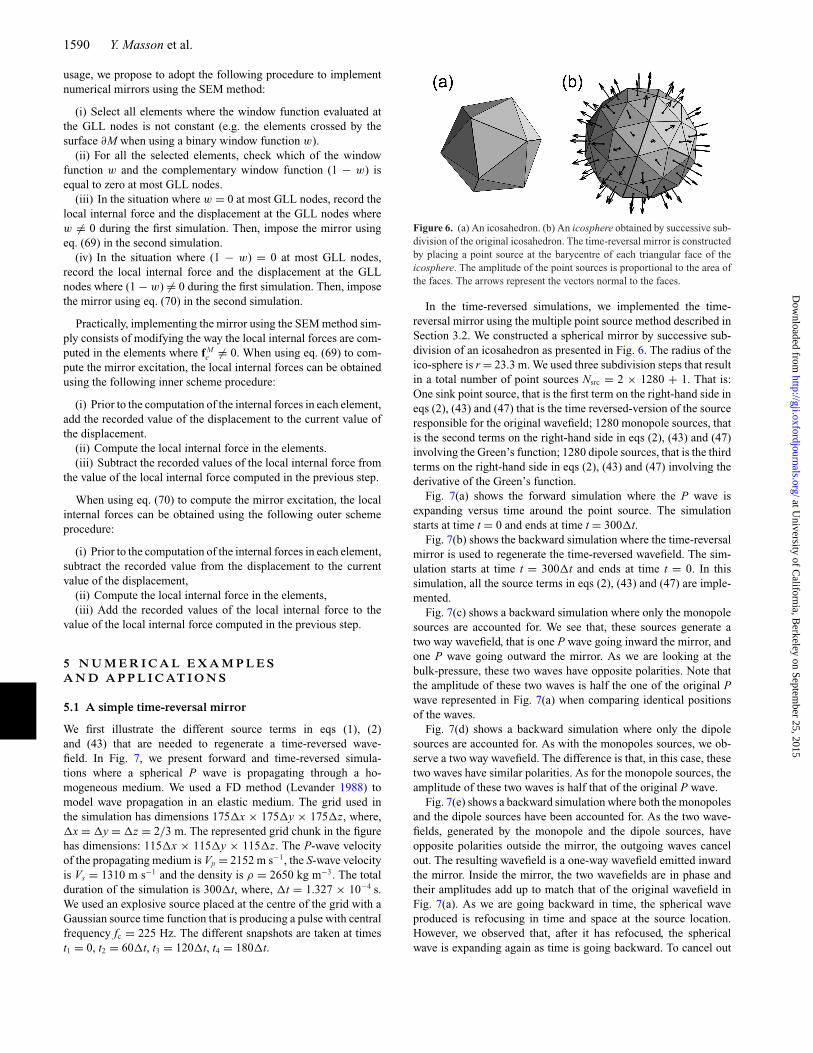
Figure 6. (a) An icosahedron. (b) An icosphere obtained by successive sub-division of the original icosahedron. The time-reversal mirror is constructedby placing a point source at the barycentre of each triangular face of theicosphere. The amplitude of the point sources is proportional to the area ofthe faces. The arrows represent the vectors normal to the faces.

In the time-reversed simulations, we implemented the time-reversal mirror using the multiple point source method described inSection 3.2. We constructed a spherical mirror by successive sub-division of an icosahedron as presented in Fig. 6. The radius of theico-sphere is r = 23.3 m. We used three subdivision steps that resultin a total number of point sources Nsrc = 2 × 1280 + 1. That is:One sink point source, that is the first term on the right-hand side ineqs (2), (43) and (47) that is the time reversed-version of the sourceresponsible for the original wavefield; 1280 monopole sources, thatis the second terms on the right-hand side in eqs (2), (43) and (47)involving the Green’s function; 1280 dipole sources, that is the thirdterms on the right-hand side in eqs (2), (43) and (47) involving thederivative of the Green’s function.

Fig. 7(a) shows the forward simulation where the P wave isexpanding versus time around the point source. The simulationstarts at time t = 0 and ends at time t = 300t.

Fig. 7(b) shows the backward simulation where the time-reversalmirror is used to regenerate the time-reversed wavefield. The sim-ulation starts at time t = 300t and ends at time t = 0. In thissimulation, all the source terms in eqs (2), (43) and (47) are imple-mented.

Fig. 7(c) shows a backward simulation where only the monopolesources are accounted for. We see that, these sources generate atwo way wavefield, that is one P wave going inward the mirror, andone P wave going outward the mirror. As we are looking at thebulk-pressure, these two waves have opposite polarities. Note thatthe amplitude of these two waves is half the one of the original Pwave represented in Fig. 7(a) when comparing identical positionsof the waves.

Fig. 7(d) shows a backward simulation where only the dipolesources are accounted for. As with the monopoles sources, we ob-serve a two way wavefield. The difference is that, in this case, thesetwo waves have similar polarities. As for the monopole sources, theamplitude of these two waves is half that of the original P wave.

Fig. 7(e) shows a backward simulation where both the monopolesand the dipole sources have been accounted for. As the two wave-fields, generated by the monopole and the dipole sources, haveopposite polarities outside the mirror, the outgoing waves cancelout. The resulting wavefield is a one-way wavefield emitted inwardthe mirror. Inside the mirror, the two wavefields are in phase andtheir amplitudes add up to match that of the original wavefield inFig. 7(a). As we are going backward in time, the spherical waveproduced is refocusing in time and space at the source location.However, we observed that, after it has refocused, the sphericalwave is expanding again as time is going backward. To cancel out

at University of C



Dow

nloaded from



Figure 7. Snapshots showing the Bulk pressure (i.e. σ xx + σ yy + σ zz) at four different instants in the forward simulation (a) and in various time-reversedsimulations (b, c, d, e, f ). The transparent sphere represents the time-reversal mirror. The grid used in the simulation has dimensions 175x × 175y × 175z,where, x = y = z = 2/3 m. The represented grid chunk in the figure has dimensions: 115x × 115y × 115z. The P-wave velocity of the propagatingmedium is Vp = 2152 m s−1, the S-wave velocity is Vs = 1310 m s−1 and the density is ρ = 2650 kg m−3. The total duration of the simulation is 300t, where,t = 1.327 × 10−4 s. We used an explosive source placed at the centre of the grid with a Gaussian source time function that is producing a pulse with centralfrequency fc = 225 Hz. The different snapshots are taken at times t1 = 0, t2 = 60t, t3 = 120t, t4 = 180t. The different time-reversed simulations illustratethe wavefields generated by the monopole, the dipole and the sink components of the mirror’s excitation. (a) Forward simulation. (b) Complete time-reversedsimulation where all the source terms are accounted for, that is, the monopole sources, the dipole sources and the sink. (c) Time-reversed simulation where onlythe monopole sources are accounted for. (d) Time-reversed simulation where only the dipole sources are accounted for. (e) Time-reversed simulation whereboth the monopole and the dipole sources are accounted for. (f) Time-reversed simulation where only the sink is accounted for.

this spherical wave propagating at negative times, one must addthe sink term represented in Fig. 7(f). We then obtain the desiredtime-reversed wavefield plotted in Fig. 7(b).

Fig. 7(f) shows a backward simulation where only the sink sourceis accounted for. It generates a one way wavefield expanding aroundthe source. It produces the same wavefield as in Fig. 7(a) but thewave front is expanding as time is going backward.

5.2 Using a time-reversal mirror to regenerate a wavefieldgoing forward in time

Fig. 8 illustrates the fact that the time-reversal mirror tool can also beused to regenerate an original wavefield going forward with respectto time.

Fig. 8(a) is similar to Fig. 7(a) and pictures the wavefield observedin the forward simulation.

The wavefield pictured in Fig. 8(b) looks similar to the one inFig. 7(b) but has been regenerated going forward in time. Interest-ingly, in that case, the mirror acts as a perfect absorbing boundary.

The simulations presented in Figs 8(c)–(f) are similar to those inFigs 7(c)–(f), respectively, but the source time functions associatedwith the monopole sources, the dipole sources and the sink sourcehave not been time reversed.

The wavefields presented in Figs 8(c) and (d) are generated bythe monopole sources an the dipole sources, respectively. Outsidethe mirror they have the same polarity, opposite to the one of theoriginal wavefield in Fig. 8(a). Inside the mirror, they have oppositepolarities. Both wavefields have the same absolute amplitudes.

at University of C



Dow

nloaded from



Figure 8. Snapshots showing the Bulk pressure (i.e. σ xx + σ yy + σ zz) at four different instants in various forward simulations. The transparent sphere representsthe time-reversal mirror. The grid used in the simulation has dimensions 175x × 175y × 175z, where, x = y = z = 2/3 m. The represented gridchunk in the figure has dimensions: 115x × 115y × 115z. The P-wave velocity of the propagating medium is Vp = 2152 m s−1, the S-wave velocity isVs = 1310 m s−1 and the density is ρ = 2650 kg m−3. The total duration of the simulation is 300t, where t = 1.327 × 10−4 s. We used an explosive sourceplaced at the centre of the grid with a Gaussian source time function that is producing a pulse with central frequency fc = 225 Hz. The different snapshots aretaken at times t1 = 0, t2 = 60t, t3 = 120t, t4 = 180t. The different simulations are comparable to the one in Fig. 7 but are not time reversed. (a) Forwardsimulation, that is with no mirror. (b) Forward simulation with the mirror and where all the source terms are accounted for, that is, the monopole sources, thedipole sources and the sink. (c) Forward simulation where only the monopole source component of the mirror are accounted for. (d) Forward simulation whereonly the dipole source component of the mirror are accounted for. (e) Forward simulation where both the monopole and the dipole source components of themirror are accounted for. (f) Forward simulation whith the time-reversed sink only.

In Fig. 8(e), we see that the wavefield generated by the monopolesources and the dipole sources taken together is a one way wave-field going outward from the mirror. This is because the twowavefields interfere destructively and constructively inside andoutside the mirror, respectively. This wavefield has the sameamplitude as the one in Fig. 8(a) but has an opposite sign.Hence, it cancels out the original wavefield as it escapes themirror.

When regenerating a wavefield going forward in time, the sinkterm is just the source itself and simply regenerates the originalwavefield as pictured in Fig. 8(f).

5.3 Using the direct discrete differentiation method toconstruct time-reversal mirrors having complex geometry

In Fig. 9, we emphasize the fact that the direct discrete differen-tiation method permits to implement time-reversal mirrors havingcomplicated geometry with ease. We used 2-D centred FDs to solvethe acoustic wave equation as discussed in Section 4.1.1. In theforward simulation, we propagated a plane wave into a randommedium obtained by smoothing a spatial realization of the whitenoise. The spatial distribution of the sound speed in the medium ispictured in the left-hand panel of Fig. 9(a). The plane wave has been

at University of C



Dow

nloaded from



Figure 9. (a) From left to right, fluctuation of the sound speed in the propagating medium, window function w(x, y) implicitly defining the time-reversal mirror,source area (i.e. grid points where the right-hand side of eqs (55) and (56) is not equal to zero). (b) Snapshot showing a plane wave propagating through themedium at three different instants (t1 = 414t, t2 = 828t, t3 = 1242t). The model has dimensions 469x × 441y, where x = y = 1 m. The totalduration of the simulation is 1300t, where, t = 2.5 × 10−4 s. (c) Snapshot showing the wavefield in (b) regenerated locally using the time-reversal mirror.

injected by forcing the acoustic pressure to match a time-varyingboundary condition at the top side of the domain. The source pulseis the derivative of a Gaussian with central frequency fc = 32 Hz.In the horizontal direction, we applied periodic boundary condi-tions to simulate an infinite medium. The model has dimensions469x × 441y, where x = y = 1 m. The total duration of thesimulation is 1300t, where, t = 2.5 × 10−4s.

In Fig. 9(b), we present three snapshots taken during the forwardsimulation at time t1 = 414t, t2 = 828t, t3 = 1242t. Weobserve that the fluctuation of the sound speed in the propagatingmedium induces a significant amount of scattering that results in acomplicated wavefield.

To construct the time-reversal mirror excitation, we first con-structed the spatial window function w pictured in the central panelof Fig. 9(a). The function w has value one inside the ‘Time’ wordand zero outside. For the ‘Reversal’ word, we smoothed the edgesof the letters so the function w goes gradually from zero to one.Inside the ‘Mirror’ word, we used a checkerboard pattern where thevalues of the function w alternate between 1/4 and 1.

During the forward simulation, we directly evaluated the right-hand side of eq. (55) and stored the value of f M at the desired gridnodes, that is the nodes where f M �= 0. These nodes are pictured

in black on the right-hand side of Fig. 9(a). At the end of thesimulation, we took a snapshot of the acoustic pressure, whichwas then multiplied by the spatial window w to obtain the initialcondition needed in the time-reversed simulation.

In the time reversed simulation, the stored values of f M were usedas the source term. The wavefield regenerated by the time-reversalmirror is pictured in Fig. 9(c). At any given point the value of theregenerated wavefield is exactly equal to the value of the originalwavefield in Fig. 9(b) multiplied by the window function in thecentral panel of Fig. 9(a). The error in the regenerated wavefield isvirtually zero as it is entirely due to round-off errors that are alsopresent in the forward wavefield.

5.4 Comparison between the direct discrete differentiationmethod and the multiple point sources method

In Fig. 10, we compare results obtained with the direct dis-crete differentiation method to results obtained with the multi-ple point sources method and when using a similar setup. Weused a FD method (Levander 1988) to model wave propaga-tion in an elastic medium. The numerical grid has dimensions:150x × 150y × 150z, where x = y = z = 2/3 m. The

at University of C



Dow

nloaded from



Figure 10. Comparison of the regenerated wavefields when using the direct discrete differentiation method and the multiple point source method. The snapshotsshows the particle velocity at three different instants. The numerical grid has dimensions: 150x × 150y × 150z, where, x = y = z = 2/3 m. Theduration of the simulations is duration of the simulation 250t, where, t = 1.327 × 10−4 s. The S-wave velocity is Vs = 1310 m s−1, the P-wave velocityis Vp = 2152 m s−1 and the density is ρ = 2650 kg m−3. We used a double couple source, located at the centre of the domain. The mirror has a sphericalshape with radius rs = 28.57 m and its centre has coordinates xs = 49.3, ys = 39.8 and zs = 49.3. (a) Forward simulation. (b) Time-reversed simulationwhere the time-reversal mirror is implemented using the direct discrete differentiation method. (c) Time-reversed simulation where the time-reversal mirror isimplemented using the multiple point sources method. (d) Same as in (c) but the number of point sources used has been reduced by a factor four.

duration of the simulations is duration of the simulation 250t,where t = 1.327 × 10−4 s. The S-wave velocity is Vs = 1310 ms−1, the P-wave velocity is Vp = 2152 m s−1 and the density isρ = 2650 kg m−3. We used a double couple source, located at thecentre of the domain, with moment tensor

M0 =

∣∣∣∣∣∣∣0 0 0

0 0 1

0 1 0

∣∣∣∣∣∣∣ . (71)

The mirror has a spherical shape with radius rs = 28.57 m. Thecentre of the sphere has coordinates xs = 49.3, ys = 39.8 and

zs = 49.3. We intently offset the centre of the mirror with respect tothe source position so that the different wavefronts are not parallelto the mirror. In addition we stopped the forward simulation at atime when some wave energy is still present inside the mirror so thatinitial conditions must be imposed in the time-reversed simulations.

The wavefield observed in the forward simulation is pictured inFig. 10(a). In Fig. 10(b), we present the result of a time reversed sim-ulation where the mirror was implemented using the direct discretedifferentiation method. The mirror was defined using a windowfunction w that takes the value one at nodes inside the sphere andthe value zero at nodes outside the sphere. To obtain the necessaryinitial conditions, we simply took a snapshot of the wavefield at

at University of C



Dow

nloaded from



the end of the forward simulation and multiplied it by the windowfunction. The wavefield presented has been obtained using the innerscheme procedure described in Section 4.1.2 to implement the mir-ror. The other schemes give similar results that are not presented.As we already discussed, the error in the regenerated wavefield isvirtually inexistent as it is entirely due to round-off errors that arealso affecting the forward wavefield.

In Fig. 10(c), we present the result of a time-reversed simulationwhere the mirror was implemented using the multiple point sourcemethod. We constructed the mirror by successive subdivision of anicosahedron as presented in Fig. 6. We used four subdivision stepsthat result in a total number of point sources Nsrc = 2 × 5120 + 1.This corresponds to an average distance d = 1.02x between twoneighbouring point sources. It corresponds to eight points per wave-length for the S wave that is roughly the minimum number of pointsper wavelength required to accurately model the propagation of Swaves. To construct the initial conditions, we defined the windowfunction

w =

∣∣∣∣∣∣∣0 ∀ φ < −l12

[1 + sin

(πφ

2l

)] ∀ −l < φ < l

1 ∀ l < φ

, (72)

where

φ(x, y, z) = rs −√

(x − xs)2 + (y − ys)2 + (z − zs)2 (73)

is the signed distance function, and l is the thickness of a layer inwhich the window function is gradually varying form zero to one.The initial conditions are obtained by taking a snapshot at the end

of the forward simulation, changing the sign of the velocity andmultiplying the stress and the velocity by the window function ineq. (72). Note that the window function w is effectively taking thevalue 1/2 on the mirror’s surface so the initial conditions match theboundary conditions in eq. (2). In this example, we observe that,when using a sufficient number of point source per wavelength,the error in the regenerated wavefield is barely visible and notproblematic.

Fig. 10(d) has been obtained in the same way as Fig. 10(c)but the number of point sources has been divided by four, thatis Nsrc = 2 × 1280 + 1. This corresponds to an average distanced = 2.03x between two neighbouring point sources. It correspondsto about four points per wavelength for the S wave that is below theminimum number of points per wavelength needed to accuratelymodel propagation of S waves with the FD method. In this situa-tion, we see that some energy is leaking out of the mirror resulting ina significant error affecting the regenerated wavefield. When com-paring the snapshots in Figs 10(c) and (d), we observe that varyingthe number of point sources used to construct the mirror permits totune the accuracy of the regenerated wavefield.

5.5 On the use of numerical mirrors for the fastcomputation of synthetic seismograms

In Fig. 11, we show that the time-reversal mirror tool, when it isused to regenerate wavefields going forward in time, permits toefficiently compute the seismic response of a medium that has been

Figure 11. Snapshots of the wavefield following an earthquake computed in a piece of Earth using a 2-D SEM method. The model spans 20 degrees andextends from the surface of the Earth to a depth of 600 km. It is divided into 6090 elements. Inside the elements, the solution is approximated using fourth-orderpolynomials. The numerical mesh allows to accurately propagate waves with periods greater than 10 s. The source time function has a central frequencyfc = 1/25 Hz, the total duration of the simulations is 3000t, where, t = 0.17 s. All the snapshots presented have been taken at time t = 1200t. We usedabsorbing boundaries, on the left, right and bottom side of the model, and a free surface on the top side. (a) Shear-wave velocity in the PREM model. (b)Shear-wave velocity anomaly that is added to the PREM model when computing the response in a perturbed model. (c) Snapshot of the wavefield observedafter an earthquake as modelled in the forward simulation. (d) Is similar to (c) but using the perturbed model obtained by adding the anomaly in (b) to thePREM model in (a). (e) Wavefield regenerated forward in time inside a mirror having a tunnel shape. (f) Same as in (e) but using the perturbed model. (g)Wavefield regenerated forward in time inside a mirror having an ellipsoidal shape. (h) Same as in (g) but using the perturbed model.

at University of C



Dow

nloaded from



perturbed locally as proposed by Robertsson & Chapman (2000)and Robertsson et al. (2000).

Fig. 11(a) shows the computational domain as well as the ref-erence earth model used for the 2-D SEM simulations. The modelspans 20 degrees and extends from the surface of the Earth’s toa depth of 600 km. it is divided into 6090 elements delimited bysolid lines. Inside the elements, the solution is approximated usingfourth-order polynomials. The numerical mesh allows to accuratelypropagate waves with periods greater than 10 s. The velocity modelemployed is the PREM model (Dziewonski et al. 1981).

Fig. 11(b) represents a velocity anomaly that is added to thereference model in Fig. 11(a) to model wave propagation in a locallyperturbed model.

Fig. 11(c) shows the wavefield following an earthquake computedusing the reference model in Fig. 11(a). The source time functionhas a central frequency fc = 1/25 Hz, the total duration of thesimulations is 3000t, where t = 0.17 s. The snapshot has beentaken at time t = 1200t. We used absorbing boundaries, on theleft, right and bottom side of the model, and a free surface on thetop side.

Fig. 11(d) is similar to Fig. 11(c) but the earth model has beenperturbed by adding the anomaly in Fig. 11(b) to the referencemodel in Fig. 11(a). When comparing Fig. 11(d) to Fig. 11(c) weobserve additional scattered waves that are due to the presence ofthe anomaly.

Fig. 11(e) shows the local regeneration of the wavefield picturedin Fig. 11(c) inside a subvolume having a tunnel shape and goingforward in time. To inject the wavefield inside the subvolume, weimplemented a time reversal mirror using the direct differentiationmethod (see Section 4.2). The model employed to model wavepropagation is the reference model in Fig. 11(a) and we observe aperfect reconstruction of the original wavefield, that is the obtainedwavefield is exactly equal to the wavefield in Fig. 11(c) inside thesubvolume delimited by the mirror and zero outside.

Fig. 11(f) has been obtained using the same procedure as inFig. 11(e), but, the perturbed model in Fig. 11(b) has been usedinstead of the reference model in Fig. 11(a) when modelling wavepropagation. In this case, we observe additional scattered wavesdue to the presence of the anomaly. Because these waves are notpart of the original wavefield, they are not cancelled out when theycross the time-reversal mirror and some energy is leaking out of thesubvolume. In fact, inside the subvolume, the regenerated wavefieldis exactly equal to the wavefield in Fig. 11(d), while, outside thesubvolume, the observed residual is exactly the difference the be-tween the wavefield computed in the perturbed model (in Fig. 11d)and the wavefield computed in the reference model (in Fig. 11c).

Figs 11(g) and (h) have been obtained exactly as Figs 11(e) and(f), respectively. The only difference is that the time-reversal mirrorused to regenerate the wavefield has an ellipsoidal shape.

Figs 11(f) and (h) illustrate the fact that, the ability to modelthe response in a locally perturbed model using the time-reversalmirror has important applications as it allows to restrict the compu-tational domain to the volume inside the mirror. For example onecan efficiently compute the response in multiple models that aresimilar outside the mirror but different inside. This, by using thetime-reversal mirror to inject the wavefield recorded in the unper-turbed model inside the region where the model has been perturbed.One can use, for example, absorbing boundaries outside the mirrorto isolate the computational domain inside the mirror.

In the situation where the sources and the receivers are locatedinside the mirror as in Fig. 11(e), one directly obtains the responsecorresponding to the perturbed model. The only part of the signal

that is lost corresponds to the wavefield that escapes the mirror andthat is backscattered inside the mirror. These may be consideredas second or higher order effects if the dimension of the mirror isappropriate. For example, the shape of the tunnel mirror in Fig. 11(e)may be obtained based on the sensitivity kernel associated with agiven seismic wave. Note that exact results could be obtained bymodifying the time-reversal mirror as proposed by van Manen et al.(2007).

In the situation where the sources and/or the receivers are locatedoutside the volume enclosed in the mirror as in Fig. 11(g), one canrecord the residual wavefield on the surface of the mirror and use awavefield extrapolation method to obtain the seismic response at thereceivers (e.g. Robertsson & Chapman 2000). The big advantageof this approach is that the wavefield in the complete unperturbedmodel only needs to be computed once. Moreover, the responseof the unperturbed model may be computed using a method thatis different from the one used to model the wavefield inside themirror. In that perspective, the proposed time-reversal mirrors arean efficient tool to develop hybrid methods where a fast solution isused for wave propagation in the larger volume outside the mirror,and an exact method is used inside the mirror.

5.6 Using time reversal mirrors for adjoint tomography

In Fig. 12, we present a time-reversed wavefield obtained using theregional SEM software RegSEM (Cupillard et al. 2012). Fig. 12(a)represents the wavefield produced by an earthquake in eastern Eu-rope. The seismic source has coordinates, 45.73◦(latitude), 26.67◦

(longitude), 93.8 Km (depth) and moment tensor

M0 =

∣∣∣∣∣∣∣1.98 −3.92 −3.88

−3.92 0.77 0.005

−3.88 0.005 −2.75

∣∣∣∣∣∣∣ · 10−17. (74)

The bandwidth of the source time function goes from 10−3 to 10−2

Hz. We used the PREM model (Dziewonski & Anderson 1981)to define the velocities and the attenuation inside the propagatingmedium.

The time-reversal mirror is implemented using the direct dis-crete differentiation method and follows the faces of the elementsto minimize the disk space usage. In the time-reversed simulation,presented in Fig. 12, the wavefield has been amplified to undo theattenuation affecting the wavefield in the forward simulation. Tokeep the time-reversed simulation stable, we used a point matchingtechnique where the wavefield is reset periodically every 1000 timesteps. As the numerical error is growing with time, when amplify-ing the wavefield in the time-reversed simulation, the regeneratedwavefield is less accurate compared to the purely elastic case. Still,the checkpointing technique permits to limit the error and nearlyperfect results can be obtained. The time-reversed simulation inFig. 12(b) can typically be run in parallel with an adjoint simula-tion (i.e. where we back propagate the misfit between the observedseismograms and the seismogram computed in the current model)to compute sensitivity kernels.

6 C O N C LU S I O N

We introduced two different methods to construct numerical equiva-lents of time-reversal mirrors. The first method is based on the directdiscrete differentiation of the original wavefield. The second methodapproximates the surface integrals in the Helmoltz-Kirchhoff rep-resentations using a set of point sources. Both methods allow us to

at University of C



Dow

nloaded from



Figure 12. Numerical example of a time-reversed simulation as it can be used, for example, in regional adjoint tomography. The magnitude of the displacementwavefield produced by an earthquake in eastern Europe is pictured. The seismic source has coordinates, 45.73◦(latitude), 26.67◦ (longitude), 93.8 Km (depth).The bandwidth of the source time function goes from 10−3 to 10−2 Hz. We used the PREM model (Dziewonski & Anderson 1981) to define the velocitiesand the attenuation inside the propagating medium. (a) Snapshot of wavefield observed after an earthquake in eastern europe modelled using the RegSEMSEM software. Note that the displacement magnitude is pictured using a logarithmic colour scale. (b) Time-reversed simulation where the wavefield in (a) isregenerated locally thanks to the time-reversal mirror.

regenerate an original wavefield locally inside a confined volumesurrounded by the time-reversal mirror. The wavefield can be re-generated equally going forward in time or backward in time. Thedirect discrete differentiation method is perfectly accurate and re-quires to store the values of the original wavefield at some specificgrid points. The multiple point source method is less grid depen-dent in the sense that the point sources can be placed off the gridnodes. While the accuracy of the multiple point source method isinferior compared to the one of the direct discrete differentiationmethod, it can be tuned by varying the number of point sourcesused to approximate the continuous integrals. We showed that theproposed time-reversal mirrors can be used to efficiently model theseismic response in a medium that has been perturbed locally. Thisopens the possibility to use the proposed mirrors to develop hybridtechniques where different methods are used to model wave propa-gation inside and outside the mirror. The present study is part of amore general effort to achieve regional scale adjoint tomography inthe deep Earth.

A C K N OW L E D G E M E N T S

The research leading to these results has received funding from theEuropean Research Council under the European Community’s Sev-enth Framework Programme (FP7-IDEAS-ERC)/ERC AdvancedGrant (WAVETOMO). The work of Paul Cupillard and Yann

Capdeville has been supported by the ANR blanche ‘meme’ grant(ANR-10-BLAN-613 MEME). We would like to thank AndreasFichtner and Johan Robertson for their interesting comment andsuggestions.

R E F E R E N C E S

Akcelik, V. et al., 2003. High resolution forward and inverse earthquakemodeling on terascale computers, in Proceedings of the 2003 ACM/IEEEConference on Supercomputing, IEEE, pp. 52–52.

Aki, K. & Richards, P.G., 1980. Quantitative Seismology, Vol. 1424,Freeman.

Alterman, Z. & Karal, F., 1968. Propagation of elastic waves in layered mediaby finite difference methods, Bull. seism. Soc. Am., 58(1), 367–398.

Bamberger, A., Chavent, G., Hemon, C. & Lailly, P., 1982. Inversion ofnormal incidence seismograms, Geophysics, 47(5), 757–770.

Baysal, E., Kosloff, D.D. & Sherwood, J.W., 1983. Reverse time migration,Geophysics, 48(11), 1514–1524.

Bednar, J.B., Bednar, C.J. & Shin, C.B., 2006. Two-way vs one-way: acase study style comparison, in Proceedings of the SEG Annual Meeting,Society of Exploration Geophysicists, New Orleans, LA.

Bielak, J., 1984. On the effective seismic input for non-linear soil-structureinteraction systems, Earthq. Eng. Struct. Dyn., 12, 107–119.

Bielak, J., Loukakis, K., Hisada, Y. & Yoshimura, C., 2003. Domain re-duction method for three-dimensional earthquake modeling in localizedregions, part I: theory, Bull. seism. Soc. Am., 93(2), 817–824.

at University of C



Dow

nloaded from



Biondi, B. & Shan, G., 2002. Prestack imaging of overturned reflections byreverse time migration, in Proceedings of the SEG Technical Program,Expanded Abstracts, Vol. 21, pp. 1284–1287.

Bouchon, M. & Sanchez-Sesma, F.J., 2007. Boundary integral equationsand boundary elements methods in elastodynamics, Adv. Geophys., 48,157–189.

Capdeville, Y., Vilotte, J. & Montagner, J., 2002. Coupling the spectralelement method with a modal solution for elastic wave propagation inglobal earth models, Geophys. J. Int., 152(1), 34–67.

Capdeville, Y., To, A. & Romanowicz, B., 2003. Coupling spectral ele-ments and modes in a spherical earth: an extension to the sandwichcase,Geophys. J. Int., 154(1), 44–57.

Capdeville, Y., Guillot, L. & Marigo, J.-J., 2010a. 1-D non-periodic ho-mogenization for the seismic wave equation, Geophys. J. Int., 181(2),897–910.

Capdeville, Y., Guillot, L. & Marigo, J.-J., 2010b. 2-D non-periodic homog-enization to upscale elastic media for p–sv waves, Geophys. J. Int., 182(2),903–922.

Capdeville, Y., Stutzmann, E., Wang, N. & Montagner, J.-P., 2013. Resid-ual homogenization for seismic forward and inverse problems in layeredmedia, Geophys. J. Int., 194(1), 470–487.

Cassereau, D. & Fink, M., 1992. Time-reversal of ultrasonic fields. III. The-ory of the closed time-reversal cavity, IEEE Trans. Ultrason., Ferroelectr.Freq. Control, 39(5), 579–592.

Chen, P., 2011. Full-wave seismic data assimilation: theoretical backgroundand recent advances, Pure appl. Geophys., 168(10), 1527–1552.

Chen, P., Zhao, L. & Jordan, T.H., 2007. Full 3D tomography for the crustalstructure of the los angeles region, Bull. seism. Soc. Am., 97(4), 1094–1120.

Clapp, R.G., 2009. Reverse time migration with random boundaries, inProceedings of the 79th Annual International Meeting, SEG ExpandedAbstracts, Vol. 28, pp. 2809–2813.

Cupillard, P., Delavaud, E., Burgos, G., Festa, G., Vilotte, J.-P., Capdeville, Y.& Montagner, J.-P., 2012. RegSEM: a versatile code based on the spectralelement method to compute seismic wave propagation at the regionalscale, Geophys. J. Int., 188, 1203–1220.

De Hoop, A.T., 1958. Representation Theorems for the Displacement in anElastic Solid and Their Application to Elastodynamic Diffraction Theory,Uitgevij Excelsior.

Dumbser, M., Kaser, M. & De La Puente, J., 2007. Arbitrary high-order finitevolume schemes for seismic wave propagation on unstructured meshes in2D and 3D, Geophys. J. Int., 171(2), 665–694.

Dziewonski, A.M. & Anderson, D.L., 1981. Preliminary reference earthmodel, Phys. Earth planet. Inter., 25(4), 297–356.

Faccioli, E., Maggio, F., Paolucci, R. & Quarteroni, A., 1997. 2D and 3Delastic wave propagation by a pseudo-spectral domain decompositionmethod, J. Seismol., 1(3), 237–251.

Fannjiang, A.C., 2009. On time reversal mirrors, Inv. Prob., 25(9), 095010.Fichtner, A., 2010. Full Seismic Waveform Modelling and Inversion,

Springer.Fichtner, A., Bunge, H.-P. & Igel, H., 2006. The adjoint method in seismol-

ogy: I. Theory, Phys. Earth planet. Inter., 157(1), 86–104.Fichtner, A., Kennett, B.L., Igel, H. & Bunge, H.-P., 2009. Full seismic

waveform tomography for upper-mantle structure in the australasian re-gion using adjoint methods, Geophys. J. Int., 179(3), 1703–1725.

Fichtner, A., Trampert, J., Cupillard, P., Saygin, E., Taymaz, T., Capdeville,Y. & Villasenor, A., 2013. Multiscale full waveform inversion, Geophys.J. Int., 194(1), 534–556.

Fink, M., 1992. Time reversal of ultrasonic fields: I. Basic principles, IEEETrans. Ultrason., Ferroelectr. Freq. Control, 39(5), 555–566.

Fink, M., 1997. Time reversed acoustics, Phys. Today, 50, 34.Fink, M. & Prada, C., 2001. Acoustic time-reversal mirrors, Inv. Prob., 17(1),

R1.Fink, M., Prada, C., Wu, F. & Cassereau, D., 1989. Self focusing in inho-

mogeneous media with time reversal acoustic mirrors, in Proceedings ofthe 1989 IEEE Trans. on Ultrasonics Symposium, IEEE, pp. 681–686.

Fletcher, R.P. & Robertsson, J.O., 2011. Time-varying boundary conditionsin simulation of seismic wave propagation, Geophysics, 76(1), A1–A6.

French, S., Lekic, V. & Romanowicz, B., 2013. Waveform tomographyreveals channeled flow at the base of the oceanic asthenosphere, Science,342(6155), 227–230.

Gauthier, O., Virieux, J. & Tarantola, A., 1986. Two-dimensional nonlinearinversion of seismic waveforms; numerical results, Geophysics, 51(7),1387–1403.

Godinho, L., Mendes, P.A., Tadeu, A., Cadena-Isaza, A., Smerzini, C.,Sanchez-Sesma, F., Madec, R. & Komatitsch, D., 2009. Numerical sim-ulation of ground rotations along 2D topographical profiles under theincidence of elastic plane waves, Bull. seism. Soc. Am., 99(2B), 1147–1161.

Griewank, A. & Walther, A., 2000. Algorithm 799: revolve: an implemen-tation of checkpointing for the reverse or adjoint mode of computationaldifferentiation, ACM Trans. Math. Software, 26(1), 19–45.

Hinze, M., Walther, A. & Sternberg, J., 2005. An optimal memory-reducedprocedure for calculating adjoints of the instationary navier-stokes equa-tions, Opt. Control Appl. Methods, 27(1), 19–40.

Hughes, T.J.R., 1987. The Finite Element Method, Linear Static and Dy-namic Finit Element Analysis, Prentice–Hall International.

Komatitsch, D., 1997. Methodes spectrales et elements spectraux pourl’equation de l’elastodynamique 2 D et 3 D en milieu heterogene, PhDthesis.

Larmat, C., Montagner, J.-P., Fink, M., Capdeville, Y., Tourin, A. &Clevede, E., 2006. Time-reversal imaging of seismic sources and ap-plication to the great sumatra earthquake, Geophys. Res. Lett., 33(19),doi:10.1029/2006GL026336.

Larmat, C., Tromp, J., Liu, Q. & Montagner, J.-P., 2008. Time rever-sal location of glacial earthquakes, J. geophys. Res., 113(B9), B09314,doi:10.1029/2008JB005607.

Lekic, V. & Romanowicz, B., 2011. Inferring upper-mantle structure by fullwaveform tomography with the spectral element method, Geophys. J. Int.,185(2), 799–831.

Levander, A., 1988. Fourth-order finite-difference pw seismograms, Geo-physics, 53(11), 1425.

Liu, Q. & Tromp, J., 2006. Finite-frequency kernels based on adjoint meth-ods, Bull. seism. Soc. Am., 96(6), 2383–2397.

Liu, Q. & Tromp, J., 2008. Finite-frequency sensitivity kernels for globalseismic wave propagation based upon adjoint methods, Geophys. J. Int.,174(1), 265–286.

Maday, Y. & Patera, A.T., 1989. Spectral element methods for the incom-pressible navier-stokes equations, in Proceedings of the State-of-the-ArtSurveys on Computational Mechanics (A90-47176 21-64). New York,American Society of Mechanical Engineers, 1989, Vol. 1, pp. 71–143.Research supported by DARPA.

Mittet, R., 1994. Implementation of the kirchhoff integral for elastic wavesin staggered-grid modeling schemes, Geophysics, 59(12), 1894–1901.

Moczo, P., Bystricky, E., Kristek, J., Carcione, J.M. & Bouchon, M., 1997.Hybrid modeling of p-sv seismic motion at inhomogeneous viscoelastictopographic structures, Bull. seism. Soc. Am., 87(5), 1305–1323.

Moczo, P., Kristek, J., Vavrycuk, V., Archuleta, R.J. & Halada, L., 2002.3D heterogeneous staggered-grid finite-difference modeling of seismicmotion with volume harmonic and arithmetic averaging of elastic moduliand densities, Bull. seism. Soc. Am., 92(8), 3042–3066.

Montagner, J.-P., Larmat, C., Capdeville, Y., Fink, M., Phung, H., Romanow-icz, B., Clevede, E. & Kawakatsu, H., 2012. Time-reversal method andcross-correlation techniques by normal mode theory: a three-point prob-lem, Geophys. J. Int., 191(2), 637–652.

Monteiller, V., Chevrot, S., Komatitsch, D. & Fuji, N., 2013. A hybridmethod to compute short-period synthetic seismograms of teleseismicbody waves in a 3-d regional model, Geophys. J. Int., 192(1), 230–247.

Mulder, W.A. & Plessix, R.-E., 2004. A comparison between one-way andtwo-way wave-equation migration, Geophysics, 69(6), 1491–1504.

Nissen-Meyer, T., Fournier, A. & Dahlen, F.A., 2007. A two-dimensionalspectral-element method for computing spherical-earth seismograms: I.Moment-tensor source, Geophys. J. Int., 168(3), 1067–1092.

Oprsal, I., Matyska, C. & Irikura, K., 2009. The source-box wave propaga-tion hybrid methods: general formulation and implementation, Geophys.J. Int., 176(2), 555–564.

at University of C



Dow

nloaded from



Patera, A.T., 1984. A spectral element method for fluid dynamics: laminarflow in a channel expansion, J. Comput. Phys., 54(3), 468–488.

Peter, D. et al., 2011. Forward and adjoint simulations of seismic wavepropagation on fully unstructured hexahedral meshes, Geophys. J. Int.,186(2), 721–739.

Plessix, R.-E., 2006. A review of the adjoint-state method for computing thegradient of a functional with geophysical applications, Geophys. J. Int.,167(2), 495–503.

Pozrikidis, C., 2005. Introduction to Finite and Spectral Element MethodsUsing MATLAB, Chapman & Hall/CRC.

Restrepo, J.M., Leaf, G.K. & Griewank, A., 1998. Circumventing storagelimitations in variational data assimilation studies, SIAM J. Sci. Comput.,19(5), 1586–1605.

Rickers, F., Fichtner, A. & Trampert, J., 2012. Imaging mantle plumes withinstantaneous phase measurements of diffracted waves, Geophys. J. Int.,190(1), 650–664.

Rickers, F., Fichtner, A. & Trampert, J., 2013. The iceland–jan mayen plumesystem and its impact on mantle dynamics in the north atlantic region:evidence from full-waveform inversion, Earth planet. Sci. Lett., 367, 39–51.

Robertsson, J.O.A. & Chapman, C.H., 2000. An efficient method for calcu-lating finite-difference seismograms after model alterations, Geophysics,65(3), 907–918.

Robertsson, J.O.A., Ryan-Grigor, S., Sayers, C.M. & Chapman, C.H., 2000.A finite-difference injection approach to modeling seismic fluid flowmonitoring, Geophysics, 65(3), 896–906.

Seriani, G., Priolo, E. & Pregarz, A., 1995. Modelling waves in anisotropicmedia by a spectral element method, in Proceedings of the Third Inter-national Conference on Mathematical and Numerical Aspects of WavePropagation, SIAM, pp. 289–298.

Snieder, R., 2002. General theory of elastic wave scattering, in Scatteringand Inverse Scattering in Pure and Applied Science, chap. 1.7.1, pp.528–542, eds Pike, R. & Sabatier, P., Academic Press.

Symes, W.W., 2007. Reverse time migration with optimal checkpointing,Geophysics, 72(5), SM213–SM221.

Tape, C., Qinya, L., Maggi, A. & Tromp, J., 2009. Adjoint tomography ofthe southern california crust, Science, 325(5943), 988–992.

Tarantola, A., 1984. Inversion of seismic reflection data in the acousticapproximation, Geophysics, 49(8), 1259–1266.

Tarantola, A., 1988. Theoretical background for the inversion of seismicwaveforms including elasticity and attenuation, Pure appl. Geophys.,128(1-2), 365–399.

To, A., Romanowicz, B., Capdeville, Y. & Takeuchi, N., 2005. 3D effects ofsharp boundaries at the borders of the African and pacific superplumes:observation and modeling, Earth planet. Sci. Lett., 233(1), 137–153.

Tromp, J., Tape, C. & Liu, Q., 2005. Seismic tomography, adjoint methods,time reversal and banana-doughnut kernels, Geophys. J. Int., 160(1), 195–216.

van Manen, D.-J., Robertsson, J. O.A. & Curtis, A., 2007. Exact wave fieldsimulation for finite-volume scattering problems, J. Acoust. Soc. Am.,122(4), EL115–EL121.

Virieux, J., 1986. P-sv wave propagation in heterogeneous media; velocity-stress finite-difference method, Geophysics, 51(4), 889–901.

Wen, L. & Helmberger, D.V., 1998. A two-dimensional P-SV hybrid methodand its application to modeling localized structures near the core-mantleboundary, J. geophys. Res., 103(B8), 17901–17918.

Whitmore, N., 1983. Iterative depth migration by backward time propa-gation, in Proceedings of the 1983 SEG Annual Meeting, Society ofExploration Geophysicists, Las Vegas, NV.

Yee, K., 1966. Numerical solution of initial boundary value problems involv-ing Maxwell’s equations in isotropic media, IEEE Trans. Anten. Propag.,14(3), 302–307.

Yoon, K., Shin, C., Suh, S., Lines, L.R. & Hong, S., 2003. 3d reverse-time migration using the acoustic wave equation: an experience with theseg/eage data set, Lead. Edge, 22(1), 38–41.

Yoon, K., Marfurt, K.J. & Starr, W., 2004. Challenges in reverse-time mi-gration, in Proceedings of the 2004 SEG Annual Meeting, Society ofExploration Geophysicists, Denver, CO.

Yoshimura, C., Bielak, J., Hisada, Y. & Fernandez, A., 2003. Domain re-duction method for three-dimensional earthquake modeling in localizedregions, part II: verification and applications, Bull. seism. Soc. Am., 93(2),825–841.

Zhao, L., Wen, L., Chen, L. & Zheng, T., 2008. A two-dimensional hybridmethod for modeling seismic wave propagation in anisotropic media,J. geophys. Res., 113(B12), B12307, doi:10.1029/2008JB005733.

Zhu, H., Bozdag, E., Peter, D. & Tromp, J., 2012. Structure of the europeanupper mantle revealed by adjoint tomography, Nat. Geosci., 5(7), 493–498.

at University of C



Dow

nloaded from


geophysical journal internationalseismo.berkeley.edu/~barbara/reprints/masson-gji2015.pdf · yder...

Documents