geometric group theory - uni-regensburg.de · why study geometric group theory? on the one hand,...
TRANSCRIPT

December 21, 2010 – 18:11
Preliminary versionPlease send corrections and suggestions to [email protected]
Clara Loh
Geometric group theory,an introduction

Clara [email protected]://www.mathematik.uni-regensburg.de/loeh/
NWF I – MathematikUniversitat Regensburg93040 RegensburgGermany
Contents
1 Introduction 1
2 Generating groups 72.1 Review of the category of groups 8
2.1.1 Axiomatic description of groups 82.1.2 Concrete groups – automorphism groups 102.1.3 Normal subgroups and quotients 13
2.2 Groups via generators and relations 152.2.1 Generating sets of groups 162.2.2 Free groups 172.2.3 Generators and relations 22
2.3 New groups out of old 282.3.1 Products and extensions 282.3.2 Free products and free amalgamated products 31
3 Groups → geometry, I: Cayley graphs 353.1 Review of graph notation 363.2 Cayley graphs 393.3 Cayley graphs of free groups 42
3.3.1 Free groups and reduced words 433.3.2 Free groups → trees 453.3.3 Trees → free groups 47
iv Contents
4 Groups → geometry, II: Group actions 494.1 Review of group actions 50
4.1.1 Free actions 514.1.2 Orbits 544.1.3 Application: Counting via group actions 58
4.2 Free groups and actions on trees 604.2.1 Spanning trees 604.2.2 Completing the proof 62
4.3 Application: Subgroups of free groups are free 664.4 The ping-pong lemma 694.5 Application: Free subgroups of matrix groups 72
5 Groups → geometry, III: Quasi-isometry 755.1 Quasi-isometry types of metric spaces 765.2 Quasi-isometry types of groups 83
5.2.1 First examples 86
5.3 The Svarc-Milnor lemma 885.3.1 Quasi-geodesics and quasi-geodesic spaces 89
5.3.2 The Svarc-Milnor lemma 91
5.3.3 Applications of the Svarc-Milnor lemma to group theory,geometry and topology 96
5.4 The dynamic criterion for quasi-isometry 1015.4.1 Applications of the dynamic criterion 107
5.5 Preview: Quasi-isometry invariants and geometric properties 1095.5.1 Quasi-isometry invariants 1095.5.2 Geometric properties of groups and rigidity 110
6 Growth types of groups 1136.1 Growth functions of finitely generated groups 1146.2 Growth types of groups 117
6.2.1 Growth types 1176.2.2 Growth types and quasi-isometry 119

1Introduction
What is geometric group theory? Geometric group theory investigates theinteraction between algebraic and geometric properties of groups:
– Can groups be viewed as geometric objects and how are geometricand algebraic properties of groups related?
– More generally: On which geometric objects can a given group act ina reasonable way, and how are geometric properties of these geometricobjects related to algebraic properties of the group in question?
How does geometric group theory work? Classically, group-valued in-variants are associated with geometric objects, such as, e.g., the isometrygroup or the fundamental group. It is one of the central insights leadingto geometric group theory that this process can be reversed to a certainextent:
1. We associate a geometric object with the group in question; thiscan be an “artificial” abstract construction or a very concrete modelspace (such as the Euclidean plane or the hyperbolic plane) or actionfrom classical geometric theories.
2. We take geometric invariants and apply these to the geometric objectsobtained by the first step. This allows to translate geometric termssuch as geodesics, curvature, volumes, etc. into group theory.Usually, in this step, in order to obtain good invariants, one restricts
2 1 Introduction
Z× Z Z Z ∗ Z
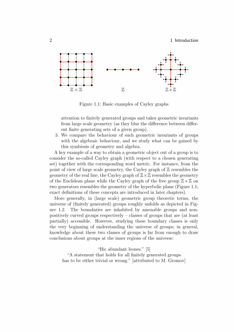
Figure 1.1: Basic examples of Cayley graphs
attention to finitely generated groups and takes geometric invariantsfrom large scale geometry (as they blur the difference between differ-ent finite generating sets of a given group).
3. We compare the behaviour of such geometric invariants of groupswith the algebraic behaviour, and we study what can be gained bythis symbiosis of geometry and algebra.
A key example of a way to obtain a geometric object out of a group is toconsider the so-called Cayley graph (with respect to a chosen generatingset) together with the corresponding word metric. For instance, from thepoint of view of large scale geometry, the Cayley graph of Z resembles thegeometry of the real line, the Cayley graph of Z×Z resembles the geometryof the Euclidean plane while the Cayley graph of the free group Z ∗ Z ontwo generators resembles the geometry of the hyperbolic plane (Figure 1.1;exact definitions of these concepts are introduced in later chapters).
More generally, in (large scale) geometric group theoretic terms, theuniverse of (finitely generated) groups roughly unfolds as depicted in Fig-ure 1.2. The boundaries are inhabited by amenable groups and non-positively curved groups respectively – classes of groups that are (at leastpartially) accessible. However, studying these boundary classes is onlythe very beginning of understanding the universe of groups; in general,knowledge about these two classes of groups is far from enough to drawconclusions about groups at the inner regions of the universe:
“Hic abundant leones.” [5]“A statement that holds for all finitely generated groups
has to be either trivial or wrong.” [attributed to M. Gromov]

3
amen
able
grou
ps
non-positivelycurved
groups
finite
grou
ps
1 Z
Abelian
nilpotent
polycyclic
solvable
elementary amenable
free groups
hyperbolic groups
CAT(0)-groups
?
Figure 1.2: The universe of groups (simplified version of Bridson’s universeof groups [5])
4 1 Introduction
Why study geometric group theory? On the one hand, geometric grouptheory is an interesting theory combining aspects of different fields of math-ematics in a cunning way. On the other hand, geometric group theory hasnumerous applications to problems in classical fields such as group theoryand Riemannian geometry.
For example, so-called free groups (an a priori purely algebraic notion)can be characterised geometrically via actions on trees; this leads to anelegant proof of the (purely algebraic!) fact that subgroups of free groupsare free.
Further applications of geometric group theory to algebra and Rieman-nian geometry include the following:
– Recognising that certain matrix groups are free groups; there is a geo-metric criterion, the so-called ping-pong-lemma, that allows to deducefreeness of a group by looking at a suitable action (not necessarilyon a tree).
– Recognising that certain groups are finitely generated; this can bedone geometrically by exhibiting a good action on a suitable space.
– Establishing decidability of the word problem for large classes of groups;for example, Dehn used geometric ideas in his algorithm solving theword problem in certain geometric classes of groups.
– Recognising that certain groups are virtually nilpotent; Gromov founda characterisation of finitely generated virtually nilpotent groups interms of geometric data, more precisely, in terms of the growth func-tion.
– Proving non-existence of Riemannian metrics satisfying certain cur-vature conditions on certain smooth manifolds; this is achieved bytranslating these curvature conditions into group theory and lookingat groups associated with the given smooth manifold (e.g., the funda-mental group). Moreover, a similar technique also yields (non-)split-ting results for certain non-positively curved spaces.
– Rigidity results for certain classes of matrix groups and Riemannianmanifolds; here, the key is the study of an appropriate geometry atinfinity of the groups involved.
– Geometric group theory provides a layer of abstraction that helps tounderstand and generalise classical geometry – in particular, in thecase of negative or non-positive curvature and the corresponding ge-ometry at infinity.

5
– The Banach-Tarski paradox (a sphere can be divided into finitelymany pieces that in turn can be puzzled together into two spherescongruent to the given one [this relies on the axiom of choice]); theBanach-Tarski paradox corresponds to certain matrix groups not be-ing “amenable”, a notion related to both measure theoretic and ge-ometric properties of groups.
– A better understanding of many classical groups; this includes, forinstance, mapping class groups of surfaces and outer automorphismsof free groups (and their behaviour similar to certain matrix groups).
Overview of the course. As the main characters in geometric grouptheory are groups, we will start by reviewing some concepts and examplesfrom group theory, and by introducing constructions that allow to generateinteresting groups. Then we will introduce one of the main combinatorialobjects in geometric group theory, the so-called Cayley graph, and reviewbasic notions concerning actions of groups. A first taste of the power ofgeometric group theory will then be presented in the discussion of geometriccharacterisations of free groups. As next step, we will introduce a metricstructure on groups via word metrics on Cayley graphs, and we will studythe large scale geometry of groups with respect to this metric structure(in particular, the concept of quasi-isometry). After that, invariants underquasi-isometry will be introduced – this includes, in particular, curvatureconditions, the geometry at infinity and growth functions. Finally, we willhave a look at the class of amenable groups and their properties.
Literature. The standard resources for geometric group theory are:– Topics in Geometric group theory by de la Harpe [12],– Metric spaces of non-positive curvature by Bridson and Haefliger [7],– Trees by Serre [19].
A short and comprehensible introduction into curvature in classical Rie-mannian geometry is given in the book Riemannian manifolds. An intro-duction to curvature by Lee [15].
Furthermore, I recommend to look at the overview articles by Bridson ongeometric and combinatorial group theory [5, 6]. The original reference formodern large scale geometry of groups is the landmark paper Hyperbolicgroups [11] by Gromov.

6 1 Introduction

2Generating groups
As the main characters in geometric group theory are groups, we will startby reviewing some concepts and examples from group theory, and by in-troducing constructions that allow to generate interesting groups. In par-ticular, we will explain how to describe groups in terms of generators andrelations, and how to construct groups via semi-direct products and amal-gamated products.

8 2 Generating groups
2.1Review
of the category of groups
2.1.1 Axiomatic description of groups
For the sake of completeness, we briefly recall the definition of a group;more information on basic properties of groups can be found in any text-book on algebra [14]. The category of groups has groups as objects andgroup homomorphisms as morhpisms.
Definition 2.1.1 (Group). A group is a set G together with a binaryoperation · : G×G −→ G satisfying the following axioms:
– Associativity. For all g1, g2, g3 ∈ G we have
g1 · (g2 · g3) = (g1 · g2) · g3.
– Existence of a neutral element. There exists a neutral element e ∈ Gfor “·”, i.e.,
∀g∈G e · g = g = g · e.
(Notice that the neutral element is uniquely determined by this prop-erty.)
– Existence of inverses. For every g ∈ G there exists an inverse ele-ment g−1 ∈ G with respect to “·”, i.e.,
g · g−1 = e = g−1 · g.
A group G is Abelian if composition is commutative, i.e., if g1 · g2 = g2 · g1
holds for all g1, g2 ∈ G.
Definition 2.1.2 (Subgroup). Let G be a group with respect to “·”. Asubset H ⊂ G is a subgroup if H is a group with respect to the restrictionof “·” to H ×H ⊂ G×G.

2.1 Review of the category of groups 9
Example 2.1.3 (Some (sub)groups).– “The” trivial group; i.e., the group consisting only of a single ele-
ment e and the composition (e, e) 7−→ e. Clearly, every group con-tains “the” trivial group given by the neutral element as subgroup.
– The sets Z, Q, and R are groups with respect to addition; moreover,Z is a subgroup of Q, and Q is a subgroup of R.
– The natural numbers N do not form a group with respect to addition(e.g., 1 does not have an additive inverse in N); the rational num-bers Q do not form a group with respect to multiplication (0 doesnot have a multiplicative inverse), but Q\{0} is a group with respectto multiplication.
– Let X be a set. Then the set SX of all bijections of type X −→ X is agroup with respect to composition of maps, the so-called symmetricgroup over X. If n ∈ N, then we abbreviate Sn := S{1,...,n}. Ingeneral, the group SX is not Abelian.
Now that we have introduced the main objects, we need morphisms torelate different objects to each other. As in other mathematical theories,morphisms should be structure preserving, and we consider two objects tobe the same if they have the same structure:
Definition 2.1.4 (Group homomorphism/isomorphism). Let G and H betwo groups.
– A map ϕ : G −→ H is a group homomorphism if ϕ is compatible withthe composition in G and H respectively, i.e., if
ϕ(g1 · g2) = ϕ(g1) · ϕ(g2)
holds for all g1, g2 ∈ G. (Notice that every group homomorphismmaps the neutral element to the neutral element).
– A group homomorphism ϕ : G −→ H is a group isomorphism if thereexists a group homomorphism ψ : H −→ G such that ϕ ◦ ψ = idH
and ψ ◦ ϕ = idG. If there exists a group isomorphism between Gand H, then G and H are isomorphic, and we write G ∼= H.
Example 2.1.5 (Some group homomorphisms).– If H is a subgroup of a group G, then the inclusion H ↪→ G is a
group homomorphism.

10 2 Generating groups
– Let n ∈ Z. Then
Z −→ Zx 7−→ n · x
is a group homomorphism; however, addition of n 6= 0 is not a grouphomomorphism (e.g., the neutral element is not mapped to the neu-tral element).
– The exponential map exp: R −→ R>0 is a group homomorphismbetween the additive group R and the multiplicative group R>0; theexponential map is even an isomorphism (the inverse homomorphismis given by the logarithm).
Definition 2.1.6 (Kernel/image of homomorphisms). Let ϕ : G −→ H bea group homomorphism. Then the subgroup
kerϕ := {g ∈ G | ϕ(g) = e}
is the kernel of ϕ, and
imϕ := {ϕ(g) | g ∈ G}
is the image of ϕ.
Remark 2.1.7 (Isomorphisms via kernel/image).1. A group homomorphism is injective if and only if its kernel is the
trivial subgroup.2. A group homomorphism is an isomorphism if and only if it is bijective.3. In particular: A group homomorphism ϕ : G −→ H is an isomor-
phism if and only if kerϕ is the trivial subgroup and imϕ = H.
Proof. Exercise.
2.1.2 Concrete groups – automorphism groups
The concept, and hence the axiomatisation, of groups developed originallyout of the observation that certain collections of “invertible” structurepreserving transformations of geometric or algebraic objects fit into the

2.1 Review of the category of groups 11
same abstract framework; moreover, it turned out that many interestingproperties of the underlying objects are encoded in the group structure ofthe corresponding automorphism group.
Example 2.1.8 (Symmetric groups). Let X be a set. Then the set of allbijections of type X −→ X forms a group with respect to composition.
This example is generic in the following sense:
Proposition 2.1.9 (Cayley’s theorem). Every group is a subgroup of somesymmetric group.
Proof. Let G be a group. For g ∈ G we define the map
fg : G −→ G
x 7−→ g · x;
looking at fg−1 shows that fg is a bijection. A straightforward computationshows that
G −→ SG
g 7−→ fg
is a group homomorphism and hence that G can be viewed as a subgroupof the symmetric group SG over G.
Example 2.1.10 (Automorphism groups). Let G be a group. Then theset Aut(G) of group isomorphisms of type G −→ G is a group with respectto composition of maps, the automorphism group of G.
Example 2.1.11 (Isometry groups/Symmetry groups). Let X be a metricspace. The set Isom(X) of all isometries of type X −→ X forms a groupwith respect to composition (a subgroup of the symmetric group SX). Forexample, in this way the dihedral groups naturally occur as symmetrygroups of regular polygons.
Example 2.1.12 (Matrix groups). Let k be a (commutative) ring (withunit), and let V be a k-module. Then the set Aut(V ) of all k-linear isomor-phisms V −→ V forms a group with respect to composition. In particular,the set GL(n, k) of invertible n × n-matrices over k is a group (with re-spect to matrix multiplication) for every n ∈ N. Similarly, also SL(n, k) isa group.

12 2 Generating groups
Example 2.1.13 (Galois groups). Let K ⊂ L be a Galois extension offields. Then the set
Gal(L/K) :={σ ∈ Aut(L)
∣∣ σ|K = idK
}of field automorphisms of L fixingK is a group with respect to composition,the so-called Galois group of the extension L/K.
Example 2.1.14 (Deck transformation groups). Let π : X −→ Y be acovering map of topological spaces. Then the set{
f ∈ map(X,X)∣∣ f is a homeomorphism with π ◦ f = π
}of Deck transformations forms a group with respect to composition.
In modern language, these examples are all instances of the followinggeneral principle: If X is an object in a category C, then the set AutC(X)of C-isomorphisms of type X −→ X is a group with respect to compositionin C.
Exercise 2.1.15 (Groups and categories).
1. Look up the definition of category, and isomorphism in a categoryand prove that automorphisms yield groups as described above.
2. What are the (natural) categories in the examples above?3. Show that, conversely, every group arises as the isomorphism group
of an object in some category.
Taking automorphism groups of geometric/algebraic objects is only oneway to associate meaningful groups to interesting objects. Over time, manygroup-valued invariants have been developed in all fields of mathematics.For example:
– fundamental groups (in topology, algebraic geometry or operator al-gebra theory, . . . )
– homology groups (in topology, algebra, algebraic geometry, operatoralgebra theory, . . . )
– . . .
2.1 Review of the category of groups 13
2.1.3 Normal subgroups and quotients
Sometimes it is convenient to ignore a certain subobject of a given objectand to focus on the remaining properties. Formally, this is done by takingquotients. In contrast to the theory of vector spaces, where the quotientof any vector space by any subspace again naturally forms a vector space,we have to be a little bit more careful in the world of groups. Only specialsubgroups lead to quotient groups :
Definition 2.1.16 (Normal subgroup). Let G be a group. A subgroup Nof G is normal if it is conjugation invariant, i.e., if
g · n · g−1 ∈ N
holds for all n ∈ N and all g ∈ G. If N is a normal subgroup of G, thenwe write N C G.
Example 2.1.17 (Some (non-)normal subgroups).– All subgroups of Abelian groups are normal.– Let τ ∈ S3 be the bijection given by swapping 1 and 2 (i.e., τ = (1 2)).
Then {id, τ} is a subgroup of S3, but it is not a normal subgroup.On the other hand, the subgroup generated by the cycle given by1 7→ 2, 2 7→ 3, 3 7→ 1 is a normal subgroup.
– Kernels of group homomorphisms are normal in the domain group;conversely, every normal subgroup also is the kernel of a certain grouphomomorphism (namely of the canonical projection to the quotient(Proposition 2.1.18)).
Proposition 2.1.18 (Quotient group). Let G be a group, and let N be asubgroup.
1. Let G/N := {g ·N | g ∈ G}, where we use the coset notation g ·N :={g · n | n ∈ N} for g ∈ G. Then the map
G/N ×G/N −→ G/N
(g1 ·N, g2 ·N) 7−→ (g1 · g2) ·N

14 2 Generating groups
is well-defined if and only if N is normal in G. If N is normalin G, then G/N is a group with respect to this composition map, theso-called quotient group of G by N .
2. Let N be normal in G. Then the canonical projection
π : G −→ G/N
g 7−→ g ·N
is a group homomorphism, and the quotient group G/N togetherwith π has the following universal property: For any group H andany group homomorphism ϕ : G −→ H with N ⊂ kerϕ there is ex-actly one group homomorphism ϕ : G/N −→ H satisfying ϕ ◦ π = ϕ:
Gϕ//
π��
H
G/Nϕ
<<zz
zz
Proof. Ad 1. Suppose that N is normal in G. In this case, the compositionmap is well-defined (in the sense that the definition does not depend onthe choice of the representatives of cosets) because: Let g1, g2, g1, g2 ∈ Gwith
g1 ·N = g1 ·N, and g2 ·N = g2 ·N.
In particular, there are n1, n2 ∈ N with g1 = g1 ·n1 and g2 = g2 ·n2. Thuswe obtain
(g1 · g2) ·N = (g1 · n1 · g2 · n2) ·N= (g1 · g2 · (g−1
2 · n1 · g2) · n2) ·N= (g1 · g2) ·N ;
in the last step we used that N is normal, which implies that g−12 ·n1 ·g2 ∈ N
and hence g−12 · n1 · g2 · n2 ∈ N . Therefore, the composition on G/N is
well-defined.That G/N indeed is a group with respect to this composition follows
easily from the fact that the group axioms are satisfied in G.Conversely, suppose that the composition on G/N is well-defined. Then
the subgroup N is normal because: Let n ∈ N and let g ∈ G. Then

2.2 Groups via generators and relations 15
g ·N = (g · n) ·N , and so (by well-definedness)
N = (g · g−1) ·N= (g ·N) · (g−1 ·N)
= ((g · n) ·N) · (g−1 ·N)
= (g · n · g−1) ·N ;
in particular, g · n · g−1 ∈ N . Therefore, N is normal in G.
Ad 2. Exercise.
Example 2.1.19 (Quotient groups).
– Let n ∈ Z. Then composition in the quotient group Z/nZ is nothingbut addition modulo n.
– The quotient group R/Z is isomorphic to the (multiplicative) circlegroup {z | z ∈ C, |z| = 1} ⊂ C \ {0}.
– The quotient of S3 by the subgroup generated by the cycle 1 7→ 2,2 7→ 3, 3 7→ 1 is isomorphic to Z/2Z.
2.2Groups via generators
and relations
How can we specify a group? One way is to construct a group as theautomorphism group of some object or as a subgroup thereof. However,when interested in finding groups with certain algebraic features, it mightin pratice be difficult to find a corresponding geometric object.
In this section, we will see that there is another – abstract – way to con-struct groups, namely by generators and relations: We will prove that forevery list of elements (“generators”) and group theoretic equations (“rela-tions”) linking these elements there always exists a group in which theserelations hold as non-trivially as possible. (However, in general, it is notpossible to decide whether the given wish-list of generators and relations

16 2 Generating groups
can be realised by a non-trivial group.) Technically, generators and rela-tions are formalised by the use of free groups and suitable quotient groupsthereof.
2.2.1 Generating sets of groups
We start by reviewing the concept of a generating set of a group; in ge-ometric group theory, one usually is only interested in finitely generatedgroups.
Definition 2.2.1 (Generating set).
– Let G be a group and let S ⊂ G be a subset. The subgroup gener-ated by S in G is the smallest subgroup (with respect to inclusion)of G that contains S; the subgroup generated by S in G is denotedby 〈S〉G.The set S generates G if 〈S〉G = G.
– A group is finitely generated if it contains a finite subset that gener-ates the group in question.
Remark 2.2.2 (Explicit description of generated subgroups). Let G bea group and let S ⊂ G. Then the subgroup generated by S in G alwaysexists and can be described as follows:
〈S〉G =⋂{H | H ⊂ G is a subgroup with S ⊂ H}
={sε11 · · · · · sεn
n
∣∣ n ∈ N, s1, . . . , sn ∈ S, ε1, . . . , εn ∈ {−1,+1}}.
Example 2.2.3 (Generating sets).
– If G is a group, then G is a generating set of G.– The trivial group is generated by the empty set.– The set {1} generates the additive group Z; moreover, also, e.g.,{2, 3} is a generating set for Z.
– Let X be a set. Then the symmetric group SX is finitely generatedif and only if X is finite (exercise).

2.2 Groups via generators and relations 17
2.2.2 Free groups
Every vector space admits special generating sets: namely those generatingsets that are as free as possible (meaning having as few linear algebraicrelations between them as possible), i.e., the linearly independent ones.Also, in the setting of group theory, we can formulate what it means to bea free generating set – however, as we will see, most groups do not admitfree generating sets. This is one of the reasons why group theory is muchmore complicated than linear algebra.
Definition 2.2.4 (Free groups, universal property). Let S be a set. Agroup F is freely generated by S if F has the following universal prop-erty: For any group G and any map ϕ : S −→ G there is a unique grouphomomorphism ϕ : F −→ G extending ϕ:
S� _
��
ϕ// G
Fϕ
??~~
~~
A group is free if it contains a free generating set.
Example 2.2.5 (Free groups).
– The additive group Z is freely generated by {1}. The additive group Zis not freely generated by {2, 3}; in particular, not every generatingset of a group contains a free generating set.
– The trivial group is freely generated by the empty set.– Not every group is free; for example, the additive groups Z/2Z and
Z2 are not free (exercise).
The term “universal property” obliges us to prove that objects havingthis universal property are unique in an appropriate sense; moreover, wewill see below (Theorem 2.2.7) that for every set there indeed exists a groupfreely generated by the given set.
Proposition 2.2.6 (Free groups, uniqueness). Let S be a set. Then, up tocanonical isomorphism, there is at most one group freely generated by S.

18 2 Generating groups
The proof consists of the standard universal-property-yoga: Namely, weconsider two objects that have the universal property in question. We thenproceed as follows:
1. We use the existence part of the universal property to obtain inter-esting morphisms in both directions.
2. We use the uniqueness part of the universal property to concludethat both compositions of these morphisms have to be the identity(and hence that both morphisms are isomorphisms).
Proof. Let F and F ′ be two groups freely generated by S. We denote theinclusion of S into F and F ′ by ϕ and ϕ′ respectively.
1. Because F is freely generated by S, the existence part of the univer-sal property of free generation guarantees the existence of a grouphomomorphism ϕ′ : F −→ F ′ such that ϕ′ ◦ ϕ = ϕ′. Analogously,there is a group homomorphism ϕ : F ′ −→ F satisfying ϕ ◦ ϕ′ = ϕ:
S� _
ϕ
��
ϕ′// F ′
Fϕ′
>>}}
}}
S� _
ϕ′
��
ϕ// F
F ′ϕ
>>}}
}}
2. We now show that ϕ ◦ ϕ′ = idF and ϕ′ ◦ ϕ = idF ′ and hence thatϕ and ϕ′ are isomorphisms: The composition ϕ ◦ ϕ′ : F −→ F is agroup homomorphism making the diagram
S� _
ϕ
��
ϕ// F
Fϕ◦ϕ′
??~~
~~
commutative. Moreover, also idF is a group homomorphism fittinginto this diagram. Because F is freely generated by S, the uniquenesspart of the universal property thus tells us that these two homomor-phisms have to coincide.
These isomorphisms are canonical in the following sense: They inducethe identity map on S, and they are (by the uniqueness part of the universalproperty) the only isomorphisms between F and F ′ extending the identityon S.

2.2 Groups via generators and relations 19
Theorem 2.2.7 (Free groups, construction). Let S be a set. Then thereexists a group freely generated by S. (By the previous proposition, thisgroup is unique up to isomorphism.)
Proof. The idea is to construct a group consisting of “words” made upof elements of S and their “inverses” using only the obvious cancellationrules for elements of S and their “inverses.” More precisely, we considerthe alphabet
A := S ∪ S,
where S := {s | s ∈ S}; i.e., S contains an element for every elementin S, and s will play the role of the inverse of s in the group that we willconstruct.
– As first step, we define A∗ to be the set of all (finite) sequences(“words”) over the alphabet A; this includes in particular the emptyword ε. On A∗ we define a composition A∗ ×A∗ −→ A∗ by concate-nation of words. This composition is associative and ε is the neutralelement.
– As second step we define
F (S) := A∗/ ∼,
where ∼ is the equivalence relation generated by
∀x,y∈A∗ ∀s∈S xssy ∼ xy,
∀x,y∈A∗ ∀s∈S xssy ∼ xy;
i.e., ∼ is the smallest equivalence relation in A∗×A∗ (with respect toinclusion) satisfying the above conditions. We denote the equivalenceclasses with respect to the equivalence relation ∼ by [ · ].It is not difficult to check that concatenation induces a well-definedcomposition · : F (S)× F (S) −→ F (S) via
[x] · [y] = [xy]
for all x, y ∈ A∗.The set F (S) together with the composition “ · ” given by concatenation
is a group: Clearly, [ε] is a neutral element for this composition, andassociativity of the composition is inherited from the associativity of the

20 2 Generating groups
composition in A∗. For the existence of inverses we proceed as follows:Inductively (over the length of sequences), we define a map I : A∗ −→ A∗
by I(ε) := ε and
I(sx) := I(x)s,
I(sx) := I(x)s
for all x ∈ A∗ and all s ∈ S. An induction shows that I(I(x)) = x and
[I(x)] · [x] = [I(x)x] = [ε]
for all x ∈ A∗ (in the last step we use the definition of ∼). This shows thatinverses exist in F (S).
The group F (S) is freely generated by S: Let i : S −→ F (S) be the mapgiven by sending a letter in S ⊂ A∗ to its equivalence class in F (S); byconstruction, F (S) is generated by the subset i(S) ⊂ F (S). As we donot know yet that i is injective, we take a little detour and first show thatF (S) has the following property, similar to the universal property of groupsfreely generated by S: For every group G and every map ϕ : S −→ G thereis a unique group homomorphism ϕ : F (S) −→ G such that ϕ ◦ i = ϕ.Given ϕ, we construct a map
ϕ∗ : A∗ −→ G
inductively by
ε 7−→ e,
sx 7−→ ϕ(s) · ϕ∗(x),
sx 7−→(ϕ(s)
)−1 · ϕ∗(x)
for all s ∈ S and all x ∈ A∗. It is easy to see that this definition of ϕ∗ iscompatible with the equivalence relation ∼ on A∗ (because it is compatiblewith the given generating set of ∼) and that ϕ∗(xy) = ϕ∗(x) · ϕ∗(y) forall x, y ∈ A∗; thus, ϕ∗ induces a well-defined map
ϕ : F (S) −→ G
[x] 7−→ [ϕ∗(x)],

2.2 Groups via generators and relations 21
which is a group homomorphism. By construction ϕ ◦ i = ϕ. Moreover,because i(S) generates F (S) there cannot be another such group homo-morphism.
In order to show that F (S) is freely generated by S, it remains to provethat i is injective (and then we identify S with its image under i in F (S)):Let s1, s2 ∈ S. We consider the map ϕ : S −→ Z given by ϕ(s1) := 1and ϕ(s2) := −1. Then the corresponding homomorphism ϕ : F (S) −→ Gsatisfies
ϕ(i(s1)
)= ϕ(s1) = 1 6= −1 = ϕ(s2) = ϕ
(i(s2)
);
in particular, i(s1) 6= i(s2). Hence, i is injective.
Depending on the problem at hand, the declarative description of freegroups via the universal property or the constructive description as in theprevious proof might be more appropriate than the other.
We conclude by collecting some properties of free generating sets in freegroups: First of all, free groups indeed are generated (in the sense of Defini-tion 2.2.1) by any free generating set (Corollary 2.2.8); second, free gener-ating sets are generating sets of minimal size (Proposition 2.2.9); moreover,finitely generated groups can be characterised as the quotients of finitelygenerated free groups (Corollary 2.2.12).
Corollary 2.2.8. Let F be a free group, and let S be a free generating setof F . Then S generates F .
Proof. By construction, the statement holds for the free group generatedby S constructed in the proof of Theorem 2.2.7; in view of the uniquenessresult Proposition 2.2.6, we obtain that also the given free group F isgenerated by S.
Proposition 2.2.9 (Rank of free groups). Let F be a free group.1. Let S ⊂ F be a free generating set of F and let S ′ be a generating set
of F . Then |S ′| ≥ |S|.2. In particular: all free generating sets of F have the same cardinality,
called the rank of F .
Proof. The first part can be derived from the universal property of freegroups (applied to homomorphisms to Z/2Z) together with a countingargument (exercise). The second part is a consequence of the first part.

22 2 Generating groups
Definition 2.2.10 (Free group Fn). Let n ∈ N and let S = {x1, . . . , xn},where x1, . . . , xn are n distinct elements. Then we write Fn for “the” groupfreely generated by S, and call Fn the free group of rank n.
Caveat 2.2.11. While subspaces of vector spaces cannot have bigger di-mension than the ambient space, free groups of rank 2 contain subgroupsthat are isomorphic to free groups of higher rank, even free subgroups of(countably) infinite rank.
Corollary 2.2.12. A group is finitely generated if and only if it is the quo-tient of a finitely generated free group, i.e., a group G is finitely generatedif and only if there exists a finitely generated free group F and a surjectivegroup homomorphism F −→ G.
Proof. Quotients of finitely generated groups are finitely generated (e.g.,the image of a finite generating set is a finite generating set of the quotient).
Conversely, let G be a finitely generated group, say generated by thefinite set S ⊂ G. Furthermore, let F be the free group generated by S;by Corollary 2.2.8, the group F is finitely generated. Using the universalproperty of F we find a group homomorphism π : F −→ G that is theidentity on S. Because S generates G and because S lies in the image of π,it follows that imπ = G.
2.2.3 Generators and relations
Free groups enable us to generate generic groups over a given set; in orderto force generators to satisfy a given list of group theoretic equations, wedivide out a suitable normal subgroup.
Definition 2.2.13 (Normal generation). Let G be a group and let S ⊂ Gbe a subset. The normal subgroup of G generated by S is the smallestnormal subgroup of G containing S; it is denoted by 〈S〉/G.
Remark 2.2.14 (Explicit description of generated normal subgroups). LetG be a group and let S ⊂ G. Then the normal subgroup generated by S

2.2 Groups via generators and relations 23
in G always exists and can be described as follows:
〈S〉/G =⋂{H | H ⊂ G is a normal subgroup with S ⊂ H}
={g1 · sε1
1 · g−11 · · · · · gn · sεn
n · g−1n∣∣ n ∈ N, s1, . . . , sn ∈ S, ε1, . . . , εn ∈ {−1,+1}, g1, . . . , gn ∈ G
}.
Example 2.2.15.– As all subgroups of Abelian groups are normal, we have 〈S〉/G = 〈S〉G
for all Abelian groups G and all subsets S ⊂ G.– We consider the symmetric group S3 and the permutation τ ∈ S3
given by swapping 1 and 2; then 〈τ〉S3 = {id{1,2,3}, τ} and 〈τ〉/S3= S3.
In the following, we use the notation A∗ for the set of (possibly empty)words in A; moreover, we abuse notation and denote elements of the freegroup F (S) over a set S by words in (S ∪ S−1)∗ (even though, strictlyspeaking, elements of F (S) are equivalence classes of words in (S ∪S−1)∗).
Definition 2.2.16 (Generators and relations). Let S be a set, and letR ⊂ (S ∪ S−1)∗ be a subset; let F (S) be the free group generated by S.Then the group
〈S |R〉 := F (S)/〈R〉/F (S)
is said to be generated by S with the relations R; if G is a group with G ∼=〈S |R〉, then 〈S |R〉 is a presentation of G.
Relations of the form “w ·w′−1” are also sometimes denoted as “w = w′”,because in the generated group, the words w and w′ represent the samegroup element.
The following proposition is a formal way of saying that 〈S |R〉 is a groupin which the relations R hold as non-trivially as possible:
Proposition 2.2.17 (Universal property of groups given by generatorsand relations). Let S be a set and let R ⊂ (S ∪ S−1)∗. The group 〈S |R〉generated by S with relations R together with the canonical map π : S −→F (S)/〈R〉/F (S) = 〈S |R〉 has the following universal property: For anygroup G and any map ϕ : S −→ G with the property that
ϕ∗(r) = e in G
24 2 Generating groups
s
t
s
t
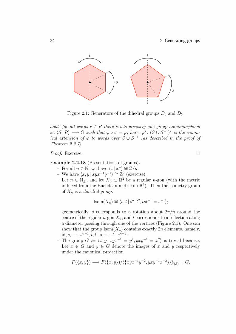
Figure 2.1: Generators of the dihedral groups D6 and D5
holds for all words r ∈ R there exists precisely one group homomorphismϕ : 〈S |R〉 −→ G such that ϕ ◦ π = ϕ; here, ϕ∗ : (S ∪ S−1)∗ is the canon-ical extension of ϕ to words over S ∪ S−1 (as described in the proof ofTheorem 2.2.7).
Proof. Exercise.
Example 2.2.18 (Presentations of groups).– For all n ∈ N, we have 〈x |xn〉 ∼= Z/n.– We have 〈x, y |xyx−1y−1〉 ∼= Z2 (exercise).– Let n ∈ N≥3 and let Xn ⊂ R2 be a regular n-gon (with the metric
induced from the Euclidean metric on R2). Then the isometry groupof Xn is a dihedral group:
Isom(Xn) ∼= 〈s, t | sn, t2, tst−1 = s−1〉;
geometrically, s corresponds to a rotation about 2π/n around thecentre of the regular n-gon Xn, and t corresponds to a reflection alonga diameter passing through one of the vertices (Figure 2.1). One canshow that the group Isom(Xn) contains exactly 2n elements, namely,id, s, . . . , sn−1, t, t · s, . . . , t · sn−1.
– The group G := 〈x, y |xyx−1 = y2, yxy−1 = x2〉 is trivial because:Let x ∈ G and y ∈ G denote the images of x and y respectivelyunder the canonical projection
F ({x, y}) −→ F ({x, y})/〈{xyx−1y−2, yxy−1x−2}〉/F (S) = G.

2.2 Groups via generators and relations 25
By definition, in G we obtain
x = x · y · x−1 · x · y−1 = y2 · x · y−1 = y · y · x · y−1 = y · x2,
and hence x = y−1. Therefore,
y−2 = x2 = y · x · y−1 = y · y−1 · y−1 = y−1,
and so x = y−1 = e. Because x and y generate G, we conclude thatG is trivial.
Caveat 2.2.19 (Word problem). The problem to determine whether agroup given by generators and relations is the trivial group is undecid-able (in the sense of computability theory); i.e., there is no algorithmicprocedure that, given generators and relations, can decide whether thecorresponding group is trivial or not.
More generally, the word problem, i.e, the problem of deciding for givengenerators and relations whether a given word in these generators repre-sents the trivial element in the corresponding group, is undecidable. Incontrast, we will see in Chapter ?? that for certain geometric classes ofgroups the word problem is solvable.
The undecidability of the word problem implies the undecidability ofmany other problems in pure mathematics.
Particularly nice presentations of groups consist of a finite generatingset and a finite set of relations:
Definition 2.2.20 (Finitely presented group). A group G is finitely pre-sented if there exists a finite generating set S and a finite set R ⊂ (S∪S−1)∗
of relations such that G ∼= 〈S |R〉.
Clearly, any finitely presented group is finitely generated. The converseis not true in general:
Example 2.2.21 (A finitely generated group that is not finitely pre-sented). The group⟨
s, t∣∣ {[tnst−n, tmst−m] | n,m ∈ Z}
⟩is finitely generated, but not finitely presented [4]. Here, we used thecommutator notation “[x, y] := xyx−1y−1.” This group is an example of aso-called lamplighter group (see also Example 2.3.5).

26 2 Generating groups
While it might be difficult to prove that a specific group is not finitelypresented (and such proofs usually require some input from algebraic topol-ogy), there is a non-constructive argument showing that there are finitelygenerated groups that are not finitely presented (Corollary 2.2.23):
Theorem 2.2.22 (Uncountably many finitely generated groups). Thereexist uncountably many isomorphism classes of groups generated by twoelements.
Before sketching de la Harpe’s proof [12, Chapter III.C] of this theorem,we discuss an important consequence:
Corollary 2.2.23. There exist uncountably many finitely generated groupsthat are not finitely presented.
Proof. Notice that there are only countably many finite presentations ofgroups, and hence that there are only countably many isomorphism typesof finitely presented groups. However, there are uncountably many finitelygenerated groups by Theorem 2.2.22.
The proof of Theorem 2.2.22 consists of two steps:1. We first show that there exists a group G generated by two elements
that contains uncountably many different normal subgroups (Propo-sition 2.2.24).
2. We then show that G even has uncountably many quotient groupsthat are pairwise non-isomorphic (Proposition 2.2.25).
Proposition 2.2.24 (Uncountably many normal subgroups). There ex-ists a group generated by two elements that has uncountably many normalsubgroups.
Sketch of proof. The basic idea is as follows: We construct a groupG gener-ated by two elements that contains a central subgroup C (i.e., each elementof this subgroup is fixed by conjugation with any other group element) iso-morphic to the additive group
⊕Z Z. The group C contains uncountably
many subgroups (e.g., given by taking subgroups generated by the subsys-tem of the unit vectors corresponding to different subsets of Z), and allthese subgroups of C are normal in G because C is central in G.

2.2 Groups via generators and relations 27
To this end we consider the group G := 〈s, t |R〉, where
R :={[
[s, tnst−n], s] ∣∣ n ∈ Z
}∪
{[[s, tnst−n], t
] ∣∣ n ∈ Z}.
Let C be the subgroup of G generated by the set {[s, tnst−n] | n ∈ Z}.All elements of C are invariant under conjugation with s by the first partof the relations, and they are invariant under conjugation with t by thesecond part of the relations; thus, C is central in G. Moreover, by care-fully inspecting the relations, it can be shown that C is isomorphic to theadditive group
⊕Z Z.
Proposition 2.2.25 (Uncountably many quotients). For a finitely gener-ated group G the following are equivalent:
1. The group G contains uncountably many normal subgroups.2. The group G has uncountably many pairwise non-isomorphic quo-
tients.
Proof. Clearly, the second statement implies the first one. Conversely, sup-pose that G has only countably many pairwise non-isomorphic quotients.
If Q is a quotient group of G, then Q is countable (as G is finitelygenerated); hence, there are only countably many group homomorphismsof type G −→ Q; in particular, there can be only countably many normalsubgroups N of G with G/N ∼= Q. Thus, in total, G can have onlycountably many different normal subgroups.
The fact that there exist uncountably many finitely generated groupscan be used for non-constructive existence proofs of groups with certainfeatures; a recent example of this type of argument is Austin’s proof ofthe existence of finitely generated groups and Hilbert modules over thesegroups with irrational von Neumann dimension (thereby answering a ques-tion of Atiyah in the negative) [3].
28 2 Generating groups
2.3
New groups out of old
In many categories, there are several ways to construct objects out of givencomponents; examples of such constructions are products and sums/push-outs. In the world of groups, these correspond to direct products and free(amalgamated) products.
In the first section, we study products and product-like constructionssuch as semi-direct products; in the second section, we discuss how groupscan be glued together, i.e., free (amalgamated) products.
2.3.1 Products and extensions
The simplest type of group constructions are direct products and theirtwisted variants, semi-direct products.
Definition 2.3.1 (Direct product). Let I be a set, and let (Gi)i∈I be afamily of groups. The (direct) product group
∏i∈I Gi of (Gi)i∈I is the group
whose underlying set is the cartesian product∏
i∈I and whose compositionis given by pointwise composition:∏
i∈I
Gi ×∏i∈I
Gi −→∏i∈I
Gi((gi)i∈I , (hi)i∈I
)7−→ (gi · hi)i∈I .
The direct product of groups has the universal property of the cate-gory theoretic product in the category of groups, i.e., homomorphisms tothe direct product group are in one-to-one correspondence to families ofhomomorphisms to all factors.
The direct product of two groups is an extension of the second factor bythe first one (taking the canonical inclusion and projection as maps):

2.3 New groups out of old 29
Definition 2.3.2 (Group extension). Let Q and N be groups. An exten-sion of Q by N is an exact sequence
1 // Ni // G
π // Q // 1
of groups, i.e., i is injective, π is surjective and im i = ker π.
Not every group extension has as extension group the direct product ofthe kernel and the quotient; for example, we can deform the direct productby introducing a twist on the kernel:
Definition 2.3.3 (Semi-direct product). Let N and Q be two groups, andlet ϕ : Q −→ Aut(N) be a group homomorphism (i.e., Q acts on N via ϕ).The semi-direct product of Q by N with respect to ϕ is the group N oϕ Qwhose underlying set is the cartesian productN×Q and whose compositionis
(N oϕ Q)× (N oϕ Q) −→ (N oϕ Q)((n1, q1), (n2, q2)
)7−→
(n1 · ϕ(q1)(n2), q1 · q2
)In other words, whenever we want to swap the positions of an element
of N with an element of Q, then we have to take the twist ϕ into account.E.g., if ϕ is the trivial homomorphism, then the corresponding semi-directproduct is nothing but the direct product.
Remark 2.3.4 (Semi-direct products and split extensions). A group ex-tension 1 // N
i // Gπ // Q // 1 splits if there exists a group ho-
momorphism s : Q −→ G such that π ◦ s = idQ. If ϕ : Q −→ Aut(N) is ahomomorphism, then
1 // Ni // N oϕ Q
π // Q // 1
is a split extension; here, i : N −→ Noϕ is the inclusion of the first com-ponent, π is the projection onto the second component, and a split is givenby
Q −→ N oϕ Q
q 7−→ (e, q).

30 2 Generating groups
Conversely, in a split extension, the extension group is a semi-direct prod-uct of the quotient by the kernel (exercise).
However, there are also group extensions that do not split; in particu-lar, not every group extension is a semi-direct product. For example, theextension
1 // Z 2· // Z // Z/2Z // 1
does not split because there is no non-trivial homomorphism from the tor-sion group Z/2Z to Z. One way to classify group extensions is to considergroup cohomology [8, 16, Chapter IV,Chapter 1.4.4].
Example 2.3.5 (Semi-direct product groups).– Let n ∈ N≥3. Then the dihedral group Dn (see Example 2.2.18) is a
semi-direct product
Dn ←→ Z/nZ oϕ Z/2Zs 7−→ ([1], 0)
t 7−→ (0, [1]),
where ϕ : Z/2Z −→ Z/nZ is given by multiplication by−1. Similarly,also the infinite dihedral group D∞ = Isom(Z) can be written asa semi-direct product of Z/2Z by Z with respect to multiplicationby −1.
– Semi-direct products of the type ZnoϕZ lead to interesting examplesof groups provided the automorphism ϕ ∈ GL(n,Z) ⊂ GL(n,R) ischosen suitably, e.g., if ϕ has interesting eigenvalues.
– Let G be a group. Then the lamplighter group over G is the semi-direct product group
(∏ZG
)oϕZ, where Z acts on the product
∏ZG
by shifting the factors:
ϕ : Z −→ Aut
(∏Z
G
)z 7−→
((gn)n∈Z 7→ (gn+z)n∈Z
)– More generally, the wreath product of two groups G and H is the
semi-direct product(∏
H G)
oϕ H, where ϕ is the shift action of Hon
∏H G. The wreath product of G and H is denoted by G oH.

2.3 New groups out of old 31
2.3.2 Free products and free amalgamated products
We now describe a construction that “glues” two groups along a commonsubgroup. In the language of category theory, glueing processes are mod-elled by the universal property of pushouts:
Definition 2.3.6 (Free product with amalgamation, universal property).Let A be a group, and let α1 : A −→ G1 and α2 : A −→ G2 be two grouphomomorphisms. A group G together with homomorphisms β1 : G1 −→ Gand β2 : G2 −→ G satisfying β1 ◦α1 = β2 ◦α2 is called an amalgamated freeproduct of G1 and G2 over A if the following universal property is satis-fied: For any group H and any two group homomorphisms ϕ1 : G1 −→ Hand ϕ2 : G2 −→ H with ϕ1 ◦ α1 = ϕ2 ◦ α2 there is exactly one homomor-phism ϕ : G −→ H of groups with ϕ ◦ β1 = ϕ ◦ β2:
G1 β1
BBB
Bϕ1
��
A
α1 >>||||
α2 BB
BBG
ϕ//___ H
G2β2
>>||||ϕ2
??
Such a free product with amalgamation is denoted by G1 ∗A G2 (see The-orem 2.3.9 for existence and uniqueness).
If A is the trivial group, then we write G1∗G2 := G1∗AG2 and call G1∗G2
the free product of G1 and G2.
Caveat 2.3.7. Notice that in general the free product with amalgamationdoes depend on the two homomorphisms α1, α2; however, usually, it isclear implicitly which homomorphisms are meant and so they are omittedfrom the notation.
Example 2.3.8 (Free (amalgamated) products).– Free groups can also be viewed as free products of several copies of
the additive group Z; e.g., the free group of rank 2 is nothing but Z∗Z(which can be seen by comparing the respective universal propertiesand using uniqueness).

32 2 Generating groups
X1 X2
A
π1(X1 ∪A X2) ∼= π1(X1) ∗π1(A) π1(X2)
Figure 2.2: The theorem of Seifert and van Kampen, schematically
– The infinite dihedral group D∞ = Isom(Z) is isomorphic to the freeproduct Z/2Z∗Z/2Z; for instance, reflection at 0 and reflection at 1/2provide generators of D∞ corresponding to the obvious generatorsof Z/2Z ∗ Z/2Z.
– The matrix group SL(2,Z) is isomorphic to the free amalgamatedproduct Z/6Z ∗Z/2Z Z/4Z [?].
– Free amalgamated products occur naturally in topology: By the the-orem of Seifert and van Kampen, the fundamental group of a spaceglued together of several components is a free amalgamated productof the fundamental groups of the components over the fundamentalgroup of the intersection (the two subspaces and their intersectionhave to be non-empty and path-connected) [17, Chapter IV] (seeFigure 2.2).
Theorem 2.3.9 (Free product with amalgamation, uniqueness and con-struction). All free products with amalgamation exist and are unique up tocanonical isomorphism.
Proof. The uniqueness proof is similar to the one that free groups areuniquely determined up to canonical isomorphism by the universal propertyof free groups (Proposition 2.2.6).
We now prove the existence of free products with amalgamation: LetA be a group and let α1 : A −→ G1 and α2 : A −→ G2 be two group

2.3 New groups out of old 33
homomorphisms. Let
G :=⟨{xg | g ∈ G1}t{xg | g ∈ G2}
∣∣ {xα1(a)xα2(a)−1 | a ∈ A}∪RG1∪RG2
⟩,
where (for j ∈ {1, 2})
RGj:= {xgxhxk
−1 | g, h, k ∈ G with g · h = k in G}.
Furthermore, we define for j ∈ {1, 2} group homomorphisms
βj : Gj −→ G
g 7−→ xg;
the relations RGjensure that βj indeed is compatible with the compositions
in Gj and G respectively. Moreover, the relations {xα1(a)xα2(a)−1 | a ∈ A}
show that β1 ◦ α1 = β2 ◦ α2.The group G (together with the homomorphisms β1 and β2) has the
universal property of the amalgamated free product of G1 and G2 over Abecause:
Let H be a group and let ϕ1 : G1 −→ H and ϕ2 : G2 −→ H be homomor-phisms with ϕ1 ◦ α1 = ϕ2 ◦ α2. We define a homomorphism ϕ : G −→ Husing the universal property of groups given by generators and relations(Proposition 2.2.17): The map on the set of all words in the genera-tors {xg | g ∈ G} t {xg | g ∈ G} and their formal inverses induced bythe map
{xg | g ∈ G1} t {xg | g ∈ G2} −→ H
xg 7−→
{ϕ1(g) if g ∈ G1
ϕ2(g) if g ∈ G2
vanishes on the relations in the above presentation of G (it vanishes on RGj
because ϕj is a group homomorphism, and it vanishes on the relations in-volving A because ϕ1 ◦ α1 = ϕ2 ◦ α2). Let ϕ : G −→ H be the homomor-phism corresponding to this map provided by said universal property.
Furthermore, by construction, ϕ ◦ β1 = ϕ1 and ϕ ◦ β2 = ϕ2.As (the image of) S := {xg | g ∈ G1} t {xg | g ∈ G2} generates G and
as any homomorphism ψ : G −→ H with ψ ◦ β1 = ϕ1 and ψ ◦ β2 = ϕ2 hasto satisfy “ψ|S = ϕ|S”, we obtain ψ = ϕ. In particular, ϕ is the uniquehomomorphism of type G −→ H with ϕ : β1 = ϕ1 and ϕ : β2 = ϕ2.

34 2 Generating groups
f
XX
π1(mapping torus of f) ∼= π1(X)∗π(f)
Figure 2.3: The fundamental group of a mapping torus, schematically
Instead of gluing two different groups along subgroups, we can also gluea group to itself along an isomorphism of two of its subgroups:
Definition 2.3.10 (HNN-extension). Let G be a group, let A, B ⊂ Gbe two subgroups, and let ϑ : A −→ B be an isomorphism. Then theHNN-extension of G with respect to ϑ is the group
G∗θ :=⟨{xg | g ∈ G} t {t}
∣∣ {t−1xat = xϑ(a) | a ∈ A} ∪RG
⟩,
whereRG := {xgxhxk
−1 | g, h, k ∈ G with g · h = k in G}.
In other words, using an HNN-extension, we can force two given sub-groups to be conjugate; iterating this construction leads to interestingexamples of groups [?]. HNN-extensions are named after G. Higman,B.H. Neumann, and H. Neumann who were the first to systematicallystudy such groups. Topologically, HNN-extensions arise naturally as fun-damental groups of mapping tori of maps that are injective on the level offundamental groups [?] (see Figure 2.3).
Remark 2.3.11 (Outlook – ends of groups). The class of (non-trivial)free amalgamated products and of (non-trivial) HNN-extensions plays animportant role in geometric group theory, more precisely, they are the keyobjects in Stallings’s classification of groups with infinitely many ends [20].

3 Groups → geometry, I:Cayley graphs
One of the central questions of geometric group theory is how groups canbe viewed as geometric objects; one way to view a (finitely generated)group as a geometric object is via Cayley graphs:
1. As first step, one associates a combinatorial structure to a group anda given generating set – the corresponding Cayley graph; this step isdiscussed in this chapter.
2. As second step, one adds a metric structure to Cayley graphs via theso-called word metrics; we will study this step in Chapter 5.
We start by reviewing some basic notation from graph theory (Sec-tion 3.1); more information on graph theory can be found in various text-books [10, 13, 9].
We then introduce Cayley graphs and discuss some basic examples ofCayley graphs (Section 3.2); in particular, we show that free groups can becharacterised combinatorially by trees: The Cayley graph of a free groupwith respect to a free generating set is a tree; conversely, if a group admitsa Cayley graph that is a tree, then (under mild additional conditions) thecorresponding generating system is a free generating system for the groupin question (Section 3.3).

36 3 Groups → geometry, I: Cayley graphs
3.1
Review of graph notation
We start by reviewing some basic notation from graph theory; in the fol-lowing, unless stated explicitly otherwise, we always consider undirected,simple graphs:
Definition 3.1.1 (Graph). A graph is a pair G = (V,E) of disjoint setswhere E is a set of subsets of V that contain exactly two elements, i.e.,
E ⊂ V [2] := {e | e ⊂ V, |e| = 2};
the elements of V are the vertices, the elements of E are the edges of G.
In other words, graphs are a different point of view on relations, andnormally graphs are used to model relations. Classical graph theory hasmany applications, mainly in the context of networks of all sorts and incomputer science (where graphs are a fundamental basic structure).
Definition 3.1.2 (Adjacent, neighbour). Let (V,E) be a graph.– We say that two vertices v, v′ ∈ V are neighbours or adjacent if they
are joined by an edge, i.e., if {v, v′} ∈ E.– The number of neighbours of a vertex is the degree of this vertex.
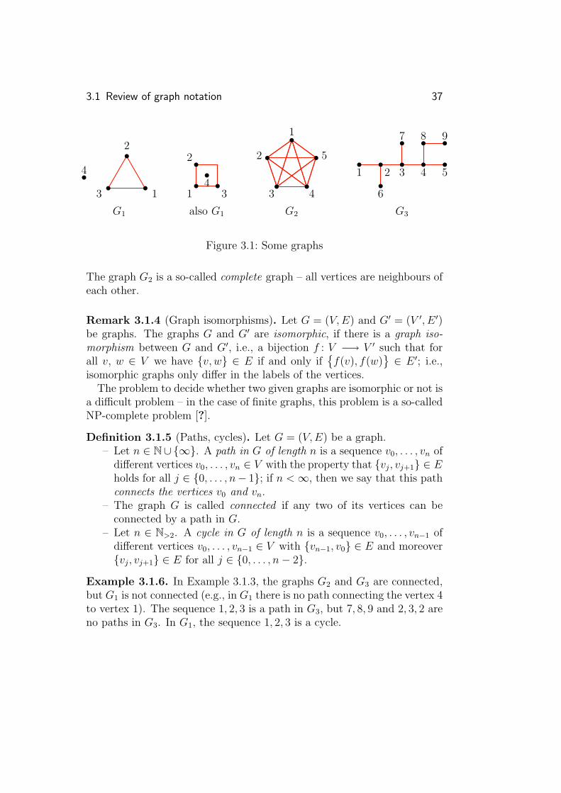
Example 3.1.3 (Graphs). Let V := {1, 2, 3, 4}, and let
E :={{1, 2}, {2, 3}, {3, 1}
}.
Then the graph G1 := (V,E) can be illustrated as in Figure 3.1; noticehowever that differently looking pictures can in fact represent the samegraph (a graph is a combinatorial object!). In G1, the vertices 2 and 3 areneighbours, while 2 and 4 are not.
Similarly, we can consider the following graphs (see Figure 3.1):
G2 :=({1, . . . , 5}, {{j, k} | j, k ∈ {1, . . . , 5}, j 6= k}
),
G3 :=({1, . . . , 9}, {{1, 2}, {2, 3}, {3, 4}, {4, 5}, {2, 6}, {3, 7}, {4, 8}, {8, 9}}
).
3.1 Review of graph notation 37
1
2
3
4
1 3
2
4
1
2
3 4
5
1 2 3 4 5
6
7 8 9
G1 also G1 G2 G3
Figure 3.1: Some graphs
The graph G2 is a so-called complete graph – all vertices are neighbours ofeach other.
Remark 3.1.4 (Graph isomorphisms). Let G = (V,E) and G′ = (V ′, E ′)be graphs. The graphs G and G′ are isomorphic, if there is a graph iso-morphism between G and G′, i.e., a bijection f : V −→ V ′ such that forall v, w ∈ V we have {v, w} ∈ E if and only if
{f(v), f(w)
}∈ E ′; i.e.,
isomorphic graphs only differ in the labels of the vertices.The problem to decide whether two given graphs are isomorphic or not is
a difficult problem – in the case of finite graphs, this problem is a so-calledNP-complete problem [?].
Definition 3.1.5 (Paths, cycles). Let G = (V,E) be a graph.– Let n ∈ N∪ {∞}. A path in G of length n is a sequence v0, . . . , vn of
different vertices v0, . . . , vn ∈ V with the property that {vj, vj+1} ∈ Eholds for all j ∈ {0, . . . , n− 1}; if n <∞, then we say that this pathconnects the vertices v0 and vn.
– The graph G is called connected if any two of its vertices can beconnected by a path in G.
– Let n ∈ N>2. A cycle in G of length n is a sequence v0, . . . , vn−1 ofdifferent vertices v0, . . . , vn−1 ∈ V with {vn−1, v0} ∈ E and moreover{vj, vj+1} ∈ E for all j ∈ {0, . . . , n− 2}.
Example 3.1.6. In Example 3.1.3, the graphs G2 and G3 are connected,but G1 is not connected (e.g., in G1 there is no path connecting the vertex 4to vertex 1). The sequence 1, 2, 3 is a path in G3, but 7, 8, 9 and 2, 3, 2 areno paths in G3. In G1, the sequence 1, 2, 3 is a cycle.

38 3 Groups → geometry, I: Cayley graphs
p
p′
v v′
Figure 3.2: Constructing a cycle (orange) out of two different paths.
Definition 3.1.7 (Tree). A tree is a connected graph that does not containany cycles. A graph that does not contain any cycles is a forest ; thus, atree is the same as a connected forest.
Example 3.1.8 (Trees). The graph G3 from Example 3.1.3 is a tree, whileG1 and G2 are not.
Proposition 3.1.9 (Characterising trees). A graph is a tree if and onlyif for every pair of vertices there exists exactly one path connecting thesevertices.
Proof. Let G be a graph such that every pair of vertices can be connectedby exactly one path in G; in particular, G is connected. Assume for acontradiction that G contains a cycle v0, . . . , vn−1. Because n > 2, the twopaths v0, vn−1 and v0, . . . , vn−1 are different, and both connect v0 with vn−1,which is a contradiction. Hence, G is a tree.
Conversely, let G be a tree; in particular, G is connected, and every twovertices can be connected by a path in G. Assume for a contradiction thatthere exist two vertices v and v′ that can be connected by two differentpaths p and p′. By looking at the first index at which p and p′ differ andat the first indices of p and p′ respectively where they meet again, we canconstruct a cycle in G (see Figure 3.2), contradicting the fact that G is atree. Hence, every two vertices of G can by connected by exactly one pathin G.

3.2 Cayley graphs 39
3.2
Cayley graphs
Given a generating set of a group, we can organise the combinatorial struc-ture given by the generating set as a graph:
Definition 3.2.1 (Cayley graph). Let G be a group and let S ⊂ G bea generating set of G. Then the Cayley graph of G with respect to thegenerating set S is the graph Cay(G,S) whose
– set of vertices is G, and whose– set of edges is {
{g, g · s}∣∣ g ∈ G, s ∈ S \ {e}}.
I.e., two vertices in a Cayley graph are adjacent if and only if they differby an element of the generating set in question.
Example 3.2.2 (Cayley graphs).– The Cayley graphs of the additive group Z with respect to the gen-
erating sets {1} and {2, 3} respectively are illustrated in Figure 3.3.Notice that when looking at these two graphs “from far away” theyseem to have the same global structure, namely they look like thereal line; in more technical terms, these graphs are quasi-isometricwith respect to the corresponding word metrics – a concept that wewill study thoroughly in later chapters (Chapter 5 ff.).
– The Cayley graph of the additive group Z2 with respect to the gen-erating set {(1, 0), (0, 1)} looks like the integer lattice in R2, see Fig-ure 3.4; when viewed from far away, this Cayley graph looks like theEuclidean plane.
– The Cayley graph of the cyclic group Z/6Z with respect to the gen-erating set {[1]} looks like a cycle graph (Figure 3.5).
– We now consider the symmetric group S3. Let τ be the transpositionexchanging 1 and 2, and let σ be the cycle 1 7→ 2, 2 7→ 3, 3 7→ 1; the

40 3 Groups → geometry, I: Cayley graphs
−2 −1 0 1 2−2 −1 0 1 2
Cay(Z, {1}
)Cay
(Z, {2, 3}
)Figure 3.3: Cayley graphs of the additive group Z
(−2,−2)
(−2,−1)
(−2, 0)
(−2, 1)
(−2, 2)
(−1,−2)
(−1,−1)
(−1, 0)
(−1, 1)
(−1, 2)
(0,−2)
(0,−1)
(0, 0)
(0, 1)
(0, 2)
(1,−2)
(1,−1)
(1, 0)
(1, 1)
(1, 2)
(2,−2)
(2,−1)
(2, 0)
(2, 1)
(2, 2)
Figure 3.4: The Cayley graph Cay(Z2, {(1, 0), (0, 1)}
)Cayley graph of S3 with respect to the generating system {τ, σ} isdepicted in Figure 3.5.Notice that the Cayley graph Cay(S3, S3) is a complete graph onsix vertices; similarly Cay(Z/6Z,Z/6Z) is a complete graph on sixvertices. In particular, we see that non-isomorphic groups may haveisomorphic Cayley graphs with respect to certain generating systems.
– The Cayley graph of a free group with respect to a free generatingset is a tree (see Theorem 3.3.1 below).
Remark 3.2.3 (Elementary properties of Cayley graphs).1. Cayley graphs are connected as every vertex g can be reached from
the vertex of the neutral element by walking along the edges corre-sponding to a presentation of g in terms of the given generators.

3.2 Cayley graphs 41
[0]
[1][2]
[3]
[4] [5]
σid
σ2
σ · ττ
σ2 · τ
Cay(Z/6Z, {[1]}
)Cay
(S3, {τ, σ}
)Cay(S3, S3)
∼= Cay(Z/6Z,Z/6Z)
Figure 3.5: Cayley graphs of Z/6Z and S3
Figure 3.6: The Petersen graph
2. Cayley graphs are regular in the sense that every vertex has the samenumber |(S ∪ S−1) \ {e}| of neighbours.
3. A Cayley graph is locally finite if and only if the generating set isfinite; a graph is said to be locally finite if every vertex has onlyfinitely many neighbours.
Exercise 3.2.4 (Petersen graph). Show that the Petersen graph (depictedin Figure 3.6), even though it is a highly regular graph, is not the Cayleygraph of any group.
Remark 3.2.5 (Cayley complexes, classifying spaces). There are higherdimensional analogues of Cayley graphs in topology: Associated with apresentation of a group, there is the so-called Cayley complex [7, Chap-ter 8A], which is a 2-dimensional object. More generally, every groupadmits a so-called classifying space, a space whose fundamental group is
42 3 Groups → geometry, I: Cayley graphs
the given group, and whose higher dimensional homotopy groups are triv-ial [?]. These spaces allow to model group theory in topology and play animportant role in the study of group cohomology [8, 16].
So far, we considered only the combinatorial structure of Cayley graphs;later, we will also consider Cayley graphs from the point of view of groupactions (most groups act freely on each of its Cayley graphs) (Chapter 4),and from the point of view of large-scale geometry, by introducing metricstructures on Cayley graphs (Chapter 5).
3.3
Cayley graphs of free groups
A combinatorial characterisation of free groups can be given in terms oftrees:
Theorem 3.3.1 (Cayley graphs of free groups). Let F be a free group,freely generated by S ⊂ F . Then the corresponding Cayley graph Cay(F, S)is a tree.
The converse is not true in general:
Example 3.3.2 (Non-free groups with Cayley trees).– The Cayley graph Cay
(Z/2Z, [1]
)consists of two vertices joined by
an edge; clearly, this graph is tree, but the group Z/2Z is not free.– The Cayley graph Cay
(Z, {−1, 1}
)coincides with Cay
(Z, {1}
), which
is a tree (looking like a line). But {−1, 1} is not a free generating setof Z.
However, these are basically the only things that can go wrong:
Theorem 3.3.3 (Cayley trees and free groups). Let G be a group and letS ⊂ G be a generating set satisfying s · t 6= e for all s, t ∈ S. If the Cayleygraph Cay(G,S) is a tree, then S is a free generating set of G.

3.3 Cayley graphs of free groups 43
While it might be intuitively clear that free generating set do not leadto any cycles in the corresponding Cayley graphs and vice versa, a formalproof requires the description of free groups in terms of reduced words(Section 3.3.1).
3.3.1 Free groups and reduced words
The construction F (S) of the free group generated by S consisted of takingthe set of all words in elements of S and their formal inverses, and takingthe quotient by a certain equivalence relation. While this construction istechnically clean and simple, it has the disadvantage that getting hold ofthe precise nature of said equivalence relation is tedious.
In the following, we discuss an alternative construction of a group freelygenerated by S by means of reduced words; it is technically a little bit morecomplicated, but has the advantage that every group element is representedby a canonical word:
Definition 3.3.4 (Reduced word). Let S be a set, and let (S ∪S)∗ be theset of words over S and formal inverses of elements of S.
– Let n ∈ N and let s1, . . . , sn ∈ S ∪ S. The word s1 . . . sn is reduced if
sj+1 6= sj and sj+1 6= sj
holds for all j ∈ {1, . . . , n− 1}. (In particular, ε is reduced.)– We write Fred(S) for the set of all reduced words in (S ∪ S)∗.
Proposition 3.3.5 (Free groups via reduced words). Let S be a set.1. The set Fred(S) of reduced words over S∪S forms a group with respect
to the composition Fred(S)× Fred(S) −→ Fred(S) given by
(s1 . . . sn, sn+1 . . . sm) 7−→ (s1 . . . sn−rsn+1+r . . . sn+m),
where s1 . . . sn and sn+1 . . . sm are elements of Fred(S), and
r := max{k ∈ {0, . . . ,min(n,m− 1)}
∣∣ ∀j∈{0,...,k−1} sn−j = sn+1+j
∨ sn−j = sn+1+j
}2. The group Fred(S) is freely generated by S.

44 3 Groups → geometry, I: Cayley graphs
x
x′
y
y′
z
z′
x · y x′ y′
(x · y) · z x′ y′ z′
y′ z′ y · z
x′ y′ z′ x · (y · z)
Figure 3.7: Associativity of the composition in Fred(S); if the reductionareas of the outer elements do not interfere
x
x′ x′′
y
y′′
z
z′z′′
x · y x′
(x · y) · z x′ z′z′′
z′ y · z
x′ x′′ z′ x · (y · z)
Figure 3.8: Associativity of the composition in Fred(S); if the reductionareas of the outer elements do interfere
Sketch of proof. Ad. 1. The above composition is well-defined because iftwo reduced words are composed, then the composed word is reduced byconstruction. Moreover, the composition has the empty word ε (which isreduced!) as neutral element, and it is not difficult to show that everyreduced word admits an inverse with respect to this composition (take theinverse sequence and flip the bar status of every element).
Thus it remains to prove that this composition is associative (whichis the ugly part of this construction): Instead of giving a formal proofinvolving lots of indices, we sketch the argument graphically (Figures 3.7and 3.8): Let x, y, z ∈ Fred(S); we want to show that (x · y) · z = x · (y · z).By definition, when composing two reduced words, we have to remove themaximal reduction area where the two words meet.
– If the reduction areas of x, y and y, z have no intersection in y, thenclearly (x · y) · z = x · (y · z) (Figure 3.7).
– If the reduction areas of x, y and y, z have a non-trivial intersection y′′

3.3 Cayley graphs of free groups 45
in y, then the equality (x · y) · z = x · (y · z) follows by carefully in-specting the reduction areas in x and z and the neighbouring regions,as indicated in Figure 3.8; notice that because of the overlap in y′′,we know that x′′ and z′′ coincide (they both are the inverse of y′′).
Ad. 2. We show that S is a free generating set of Fred(S) by verifying thatthe universal property is satsified: So let H be a group and let ϕ : S −→ Hbe a map. Then a straightforward (but slightly technical) computationshows that
ϕ := ϕ∗|Fred(S) : Fred(S) −→ H
is a group homomorphism (recall that ϕ∗ is the extension of ϕ to theset (S ∪ S)∗ of all words). Clearly, ϕ|S = ϕ; because S generates Fred(S)it follows that ϕ is the only such homomorphism. Hence, Fred(S) is freelygenerated by S.
As a corollary to the proof of the second part, we obtain:
Corollary 3.3.6. Let S be a set. Any element of F (S) = (S ∪S)∗/ ∼ canbe represented by exactly one reduced word over S ∪ S.
Corollary 3.3.7. The word problem in free groups is solvable – we justneed to consider and compare reduced words.
Remark 3.3.8 (Reduced words in free products etc.). Using the samemethod of proof, one can describe free products G1 ∗ G2 of groups G1
and G2 by reduced words; in this case, one calls a word
g1 . . . gn ∈ (G1 tG2)∗
with n ∈ N and g1, . . . , gn ∈ G1 tG2 reduced, if for all j ∈ {1, . . . , n− 1}– either gj ∈ G1 \ {e} and gj+1 ∈ G2 \ {e},– or gj ∈ G2 \ {e} and gj+1 ∈ G1 \ {e}.
Similarly, one can also describe free amalgamated products and HNN-extensions by suitable classes of reduced words [19, Chapter I].
3.3.2 Free groups → trees
Proof of Theorem 3.3.1. Suppose the group F is freely generated by S. ByProposition 3.3.5, the group F is isomorphic to Fred(S) via an isomorphism

46 3 Groups → geometry, I: Cayley graphs
gn−1
g0
g1 g2
sn
s1
s2
gn−1
g0
g1 g2
ϕ(sn)
ϕ(s1)
ϕ(s2)
(a) (b)
Figure 3.9: Cycles lead to reduced words, and vice versa
that is the identity on S; without loss of generality we can therefore assumethat F is Fred(S).
We now show that then the Cayley graph Cay(F, S) is a tree: Because Sgenerates F , the graph Cay(F, S) is connected. Assume for a contradictionthat Cay(F, S) contains a cycle g0, . . . , gn−1 of length n with n ≥ 3; inparticular, the elements g0, . . . , gn−1 are distinct, and
sj+1 := gj+1 · gj−1 ∈ S ∪ S−1
for all j ∈ {0, . . . , n − 2}, as well as sn := g0 · gn−1−1 ∈ S ∪ S−1 (Fig-
ure 3.9 (a)). Because the vertices are distinct, the word s0 . . . sn−1 is re-duced; on the other hand, we obtain
sn . . . s1 = g0 · gn−1−1 · · · · · g2 · g1
−1 · g1 · g0−1 = e = ε
in F = Fred(S), which is impossible. Therefore, Cay(F, S) cannot containany cycles. So Cay(F, S) is a tree.
Example 3.3.9 (Cayley graph of the free group of rank 2). Let S be a setconsisting of two different elements a and b. Then the corresponding Cayleygraph Cay
(F (S), {a, b}
)is a regular tree whose vertices have exactly four
neighbours (see Figure 3.10).

3.3 Cayley graphs of free groups 47
ε a
ab
ab−1
a2
b ba
Figure 3.10: Cayley graph of the free group of rank 2 with respect to a freegenerating set {a, b}
3.3.3 Trees → free groups
Proof of Theorem 3.3.3. Let G be a group and let S ⊂ G be a reducedgenerating set such that the corresponding Cayley graph Cay(G,S) is atree. In order to show that then S is a free generating set of G, in viewof Proposition 3.3.5, it suffices to show that G is isomorphic to Fred(S) viaan isomorphism that is the identity on S.
Because Fred(S) is freely generated by S, the universal property of freegroups provides us with a group homomorphism ϕ : Fred(S) −→ G that isthe identity on S. As S generates G, it follows that ϕ is surjective. Assumefor a contradiction that ϕ is not injective. Let s1 . . . sn ∈ Fred(S) \ {ε}with s1, . . . , sn ∈ S ∪ S be an element of minimal length that is mappedto e by ϕ. We consider the following cases:
– Because ϕ|S = idS is injective, it follows that n > 1.– If n = 2, then it would follow that
e = ϕ(s1 · s2) = ϕ(s1) · ϕ(s2) = s1 · s2
in G, contradicting that s1 . . . sn is reduced and that s · t 6= e for

48 3 Groups → geometry, I: Cayley graphs
all s, t ∈ S.– If n ≥ 3, we consider the sequence g0, . . . , gn−1 of elements of G given
inductively by g0 := e and
gj+1 := gj · ϕ(sj+1)
for all j ∈ {0, . . . , n−2} (Figure 3.9 (b)). The sequence g0, . . . , gn−1 isa cycle in Cay(G,S) because by minimality of the word s1 . . . sn, theelements g0, . . . , gn−1 are all distinct; moreover, Cay(G,S) containsthe edges {g0, g1}, . . . , {gn−2, gn−1}, and the edge
{gn−1, g0} = {s1 · s2 · · · · · sn−1, e}= {s1 · s2 · · · · · sn−1, s1 · s2 · · · · · sn}.
However, this contradicts that Cay(G,S) is a tree.Hence, ϕ : Fred(S) −→ G is injective.
4 Groups → geometry, II:Group actions
In the previous chapter, we took the first step from groups to geometryby considering Cayley graphs. In the present chapter, we consider anothergeometric aspect of groups by looking at so-called group actions, which canbe viewed as a generalisation of seeing groups as symmetry groups. Westart by reviewing some basic concepts about group actions (Section 4.1).Further introductory material on group actions and symmetry can be foundin Armstrong’s book [2].
As we have seen, free groups can be characterised combinatorially as thegroups admitting trees as Cayley graphs (Section 3.3). In Section 4.2, wewill prove that this characterisation can be generalised to a first geometriccharacterisation of free groups: A group is free if and only if it admits afree action on a tree. An important consequence of this characterisation isthat it leads to an elegant proof of the fact that subgroups of free groupsare free – which is a purely algebraic statement! (Section 4.3).
Another tool helping us to recognise that certain groups are free is theso-called ping-pong lemma (Section 4.4); this is particularly useful to provethat certain matrix groups are free – which also is a purely algebraic state-ment (Section 4.5).
50 4 Groups → geometry, II: Group actions
4.1
Review of group actions
Recall that for an object X in a category C the set AutC(X) of all C-auto-morphisms of X is a group with respect to composition in the category C.
Definition 4.1.1 (Group action). Let G be a group, let C be a category,and let X be an object in C. An action of G on X in the category C isa group homomorphism G −→ AutC(X). In other words, a group actionof G on X consists of a family (fg)g∈G of automorphisms of X such that
fg ◦ fh = fg·h
holds for all g, h ∈ G.
Example 4.1.2 (Group actions, generic examples).– Every group G admits an action on any object X in any category C,
namely the trivial action:
G −→ AutC(X)
g 7−→ idX .
– If X is an object in a category C, the automorphism group AutC(X)canonically acts on X via the homomorphism
idAutC(X) : AutC(X) −→ AutC(X).
In other words: group actions are a concept generalising automor-phism/symmetry groups.
– Let G be a group and let X be a set. If % : G −→ AutSet(X) is anaction of G on X by bijections, then we also use the notation
g · x :=(%(g)
)(x)
for g ∈ G and x ∈ X, and we can view % as a map G×X −→ X.

4.1 Review of group actions 51
More generally, we also use this notation whenever the group G ac-tions on an object in a category, where morphisms are maps of setsand the composition of morphisms is nothing but composition ofmaps. This applies for example to
– actions by isometries on a metric space,– actions by homeomorphisms on a topological space,– . . .
– Further examples of group actions are actions of groups on a topo-logical space by homotopy equivalences or actions on a metric spaceby quasi-isometries (see Chapter 5); notice however, that in thesecases, automorphisms are equivalence classes of maps of sets andcomposition of morphisms is done by composing representatives ofthe corresponding equivalence classes.
– An action of a group on a vector space by linear isomorphisms iscalled a representation of the group in question.
On the one hand, group actions allow us to understand groups betterby looking at suitable objects on which the groups act; on the other hand,group actions also allow us to understand geometric objects better by look-ing at groups that can act nicely on these objects.
4.1.1 Free actions
The relation between groups and geometric objects acted upon is par-ticularly strong if the group action is a so-called free action. Importantexamples of free actions are the natural actions of groups on their Cayleygraphs (provided the group does not contain any elements of order 2), andthe action of the fundamental group of a space on its universal covering.
Definition 4.1.3 (Free action on a set). Let G be a group, let X be a set,and let G×X −→ X be an action of G on X. This action is free if
g · x 6= x
holds for all g ∈ G \ {e} and all x ∈ X. In other words, an action is free ifand only if every non-trivial group element acts without fixed points.

52 4 Groups → geometry, II: Group actions
R
universal covering map
S1
Figure 4.1: Universal covering of S1
Example 4.1.4 (Left translation action). If G is a group, then the lefttranslation action
G −→ Aut(G)
g 7−→ (h 7→ g · h)
is a free action of G on itself by bijections.
Example 4.1.5 (Rotations on the circle). Let S1 := {z ∈ C | |z| = 1} bethe unit circle in C, and let α ∈ R. Then the rotation action
Z× S1 −→ S1
(n, z) 7−→ e2πi·α·n · z
of Z on S1 is free if and only if α is irrational.
Example 4.1.6 (Isometry groups). In general, the action of an isometrygroup on its underlying geometric object is not necessarily free: For exam-ple, the isometry group of the unit square does not act freely on the unitsquare – e.g., the vertices of the unit square are fixed by reflections alonga diagonal.
4.1 Review of group actions 53
Example 4.1.7 (Universal covering). Let X be a “nice” path-connectedtopological space (e.g., a CW-complex). Associated with X there is a so-
called universal covering space X, a path-connected space covering X thathas trivial fundamental group.
The fundamental group π1(X) can be identified with the deck transfor-
mation group of the universal covering X −→ X and the action of π1(X)
on X by deck transformations is free (and properly discontinuous).E.g., the fundamental group of S1 is isomorphic to Z, the universal
covering of S1 is the exponential map R −→ S1, and the action of thefundamental group of S1 on R is given by translation (Figure 4.1).
There are two natural definitions of free actions on graphs – one thatrequires that no vertex and no edge is fixed by any non-trivial group ele-ment and one that only requires that no vertex is fixed. We will use thefirst, stronger, one:
Definition 4.1.8 (Free action on a graph). Let G be a group acting on agraph (V,E) by graph isomorphisms via % : G −→ Aut(V,E). The action %is free if for all g ∈ G \ {e} we have
∀v∈V
(%(g)
)(v) 6= v, and
∀{v,v′}∈E
(%(g)
)({v, v′}
)6= {v, v′}.
Example 4.1.9 (Action on Cayley graphs). Let G be a group and let Sbe a generating set of G. Then the group G acts by graph isomorphismson the Cayley graph Cay(G,S) via left translation:
G −→ Aut(Cay(G,S)
)g 7−→ `g := (h 7→ g · h);
notice that this map is indeed well-defined and a group homomorphism.
Proposition 4.1.10 (Free actions on Cayley graphs). Let G be a groupand let S be a generating set of G. Then the left translation action onthe Cayley graph Cay(G,S) is free if and only if S does not contain anyelements of order 2.
Recall that the order of a group element g of a group G is the infinimumof all n ∈ N>0 with gn = e; here, we use the convention inf ∅ :=∞.

54 4 Groups → geometry, II: Group actions
Proof. The action on the vertices is nothing but the left translation actionby G on itself, which is free. It therefore suffices to study under whichconditions the action of G on the edges is free:
If the action of G on the edges of the Cayley graph Cay(G,S) is not free,then S contains an element of order 2: Let g ∈ G, and let {v, v′} be anedge of Cay(G,S) with {v, v′} = g · {v, v′} = {g · v, g · v′}; by definition,we can write v′ = v · s with s ∈ S ∪ S−1 \ {e}. Then one of the followingcases occurs:
1. We have g · v = v and g · v′ = v′. Because the action of G on thevertices is free, this is equivalent to g = e.
2. We have g · v = v′ and g · v′ = v. Then in G we have
v = g · v′ = g · (v · s) = (g · v) · s = v′ · s = (v · s) · s = v · s2
and so s2 = e. As s 6= e, it follows that S contains an element oforder 2.
Conversely, if s ∈ S has order 2, then s fixes the edge {e, s} = {s2, s}of Cay(G,S).
4.1.2 Orbits
A group action can be disassembled into orbits, leading to the orbit spaceof the action. Conversely, one can try to understand the whole object bylooking at the orbit space and the orbits/stabilisers.
Definition 4.1.11 (Orbit). Let G be a group acting on a set X.
– The orbit of an element x ∈ X with respect to this action is the set
G · x := {g · x | g ∈ G}.
– The quotient of X by the given G-action (or orbit space) is the set
G \X := {G · x | x ∈ X}
of orbits; we write “G \X” because G acts “from the left.”

4.1 Review of group actions 55
0
z
S1 · z
Figure 4.2: Orbits of the rotation action of S1 on C
In a sense, the orbit space describes the original object “up to symmetry”or “up to irrelevant transformations.”
If a group does not only act by bijections on a set, but if the set isequipped with additional structure that is preserved by the action (e.g., anaction by isometries on a metric space), then usually also the orbit spaceinherits additional structure similar to the one on the space acted upon.However, in general, the orbit space is not as well-behaved as the originalspace; e.g., the quotient space of an action on a metric space by isometriesin general is only a pseudo-metric space – even if the action is free (e.g.,this happens for irrational rotations on the circle).
Example 4.1.12 (Rotation on C). We consider the action of the unitcircle S1 (which is a group with respect to multiplication) on the complexnumbers C given by multiplication of complex numbers. The orbit of theorigin 0 is just {0}; the orbit of an element z ∈ C\{0} is the circle around 0passing through z (Figure 4.2). The quotient of C by this action can beidentified with R≥0 (via the absolute value).
Example 4.1.13 (Universal covering). Let X be a “nice” path-connectedtopological space (e.g., a CW-complex). The quotient of the universal cov-
ering X by the action of the fundamental group π1(X) by deck transfor-mations is homeomorphic to X.
Definition 4.1.14 (Stabiliser, fixed set). Let G be a group acting on aset X.

56 4 Groups → geometry, II: Group actions
– The stabiliser group of an element x ∈ X with respect to this actionis given by
Gx := {g ∈ G | g · x = x};notice that Gx indeed is a group (a subgroup of G).
– The fixed set of an element g ∈ G is given by
Xg := {x ∈ X | g · x = x};
more generally, if H ⊂ G is a subset, then we write XH :=⋂
h∈H Xh.
– We say that the action of G on X has a global fixed point, if XG 6= ∅.
Example 4.1.15 (Isometries of the unit square). Let Q be the (filled) unitsquare in R2, and let G be the isometry group of Q with respect to theEuclidean metric on R2. Then G naturally acts on Q by isometries and weknow that G ∼= D4.
– Let t ∈ G be the reflection along the diagonal passing through (0, 0)and (1, 1). Then
Qt ={(x, x)
∣∣ x ∈ [0, 1]}.
– Let s ∈ G be rotation around 2π/4. Then
Qs = {(1/2, 1/2)}.
– The orbit of (0, 0) are all four vertices of Q, and the stabiliser of (0, 0)is G(0,0) = {idQ, t}.
– The stabiliser of (1/3, 0) is the trivial group.– The stabiliser of (1/2, 1/2) is G(1/2,1/2) = G, so (1/2, 1/2) is a global
fixed point of this action.
Proposition 4.1.16 (Actions of finite groups on trees). Any action of afinite group on a (non-empty) tree has a global fixed point (in the sense thatthere is a vertex fixed by all group elements or an edge fixed by all groupelements).
Proof. Exercise. [We look at a vertex such that the diameter of the cor-responding orbit is minimal. If there is no globally fixed vertex or edge,then this minimal diameter is at least 2. We now consider the vertices ofsuch a minimal orbit and all paths connecting them. Using the uniquenessof paths in trees (Proposition 3.1.9) one can then find a vertex on thesepaths whose orbit has smaller diameter, contradicting minimality.]

4.1 Review of group actions 57
Proposition 4.1.17 (Counting orbits). Let G be a group acting on aset X.
1. If x ∈ X, then the map
Ax : G/Gx −→ G · xg ·Gx 7−→ g · x
is well-defined and bijective. Here, G/Gx denotes the set of all Gx-co-sets in G, i.e., G/Gx = {g ·Gx | g ∈ G}.
2. Moreover, the number of distinct orbits equals the average number ofpoints fixed by a group element: If G and X are finite, then
|G \X| = 1
|G|·∑g∈G
|Xg|.
Proof. Ad 1. We start by showing that Ax is well-defined, i.e., that thedefinition does not depend on the chosen representatives in G/Gx: Letg1, g2 ∈ G with g1·Gx = g2·Gx. Then there exists an h ∈ Gx with g1 = g2·h.By definition of Gx, we then have g1 · x = (g2 · h) · x = g2 · (h · x) = g2 · x;thus, Ax is well-defined.
By construction, the map Ax is surjective. Why is Ax injective? Letg1, g2 ∈ G with g1 · x = g2 · x. Then (g−1
1 · g2) · x = x and so g−11 · g2 ∈ Gx.
Therefore, g1 ·G1 = g1 · (g−11 · g2) ·Gx = g2 ·Gx. Hence, Ax is injective.
Ad 2. This equality is proved by double counting: More precisely, weconsider the set
F := {(g, x) | g ∈ G, x ∈ X, g · x = x} ⊂ G×X.
By definition of stabiliser groups and fixed sets, we obtain∑x∈X
|Gx| = |F | =∑g∈G
|Xg|.
We now transform the right hand side: Notice that |G/Gx| · |Gx| = |G|because every coset of Gx in G has the same size as Gx; therefore, using

58 4 Groups → geometry, II: Group actions
Figure 4.3: The same punchcard seen from different sides/angles
the first part, we obtain
∑x∈X
|Gx| =∑x∈X
|G||G/Gx|
=∑x∈X
|G||G · x|
=∑
G·x∈G\X
∑y∈G·x
|G||G · x|
=∑
G·x∈G\X
|G · x| · |G||G · x|
= |G \X| · |G|.
4.1.3 Application: Counting via group actions
Group actions can be used to solve certain counting problems. A standardexample from algebra is the proof of the Sylow theorems in finite grouptheory: in this proof, the conjugation action of a group on the set of certainsubgroups is considered [2, Chapter 20].
Another class of examples arises in combinatorics:
Example 4.1.18 (Counting punchcards [1]). How many 3×3-punchcardswith exactly two holes are there, if front and back sides of the punchcardsare not distinguishable, and also all vertices are indistinguishable? Forexample, the punchcards depicted in Figure 4.3 are all considered to bethe same.
In terms of group actions, this question can be reformulated as follows:
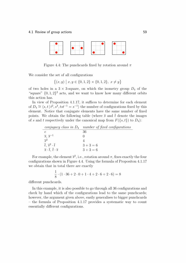
4.1 Review of group actions 59
Figure 4.4: The punchcards fixed by rotation around π
We consider the set of all configurations{(x, y)
∣∣ x, y ∈ {0, 1, 2} × {0, 1, 2}, x 6= y}
of two holes in a 3 × 3-square, on which the isometry group D4 of the“square” {0, 1, 2}2 acts, and we want to know how many different orbitsthis action has.
In view of Proposition 4.1.17, it suffices to determine for each elementof D4
∼= 〈s, t | t2, s4, tst−1 = s−1〉 the number of configurations fixed by thiselement. Notice that conjugate elements have the same number of fixedpoints. We obtain the following table (where s and t denote the imagesof s and t respectively under the canonical map from F ({s, t}) to D4):
conjugacy class in D4 number of fixed configurationse 36s, s−1 0s2 4t, s2 · t 3 + 3 = 6s · t, t · s 3 + 3 = 6
For example, the element s2, i.e., rotation around π, fixes exactly the fourconfigurations shown in Figure 4.4. Using the formula of Propositon 4.1.17we obtain that in total there are exactly
1
8· (1 · 36 + 2 · 0 + 1 · 4 + 2 · 6 + 2 · 6) = 8
different punchcards.
In this example, it is also possible to go through all 36 configurations andcheck by hand which of the configurations lead to the same punchcards;however, the argument given above, easily generalises to bigger punchcards– the formula of Proposition 4.1.17 provides a systematic way to countessentially different configurations.

60 4 Groups → geometry, II: Group actions
4.2Free groups
and actions on trees
In this section, we show that free groups can be characterised geometricallyvia free actions on trees; recall that for a free action of a group on agraph no non-trivial group element is allowed to fix any vertices or edges(Definition 4.1.8).
Theorem 4.2.1 (Free groups and actions on trees). A group is free if andonly if it admits a free action on a (non-empty) tree.
Proof of Theorem 4.2.1, part I. Let F be a free group, freely generatedby S ⊂ F ; then the Cayley graph Cay(F, S) is a tree by Theorem 3.3.1.We now consider the left translation action of F on Cay(F, S).
Applying the universal property of F with respect to the free generatingsystem S to maps S −→ Z it is easily seen that S cannot contain anyelement of order 2; therefore, the left translation action of F on Cay(F, S)is free by Proposition 4.1.10.
Conversely, suppose that a group G acts freely on a tree T . How can weprove that G has to be free? Roughly speaking, we will show that out of Tand the G-action on T we can construct – by contracting certain subtrees– a tree that is a Cayley graph of G for a suitable generating set and suchthat the assumptions of Theorem 3.3.3 are satisfied. This allows us todeduce that the group G is free.
The subtrees that will be contracted are so-called spanning trees, whichwe will discuss in the following section.
4.2.1 Spanning trees
Trees are the simplest and best accessible type of graphs. In many appli-cations, one therefore wants to approximate graphs by trees. One, crude,approximation is given by spanning trees:

4.2 Free groups and actions on trees 61
Figure 4.5: A spanning tree (red) for a shift action of Z
Definition 4.2.2 (Spanning tree). Let G be a group acting on a connectedgraph X by graph automorphisms. A spanning tree of this action is asubtree of X that contains exactly one vertex of every orbit of the inducedG-action on the vertices of X.
A subgraph of a graph (V,E) is a graph (V ′, E ′) with V ′ ⊂ V and E ′ ⊂ E;a subgraph is a subtree if it is in addition a tree.
Example 4.2.3 (Spanning trees). We consider the action of Z by “hori-zontal” shifting on the (infinite) tree depicted in Figure 4.5. Then the redsubgraph is a spanning tree for this action.
Theorem 4.2.4 (Existence of spanning trees). Every action of a group ona connected graph by graph automorphisms admits a spanning tree.
Proof. Let G be a group acting on a connected graph X. In the following,we may assume that X is non-empty (otherwise the empty tree is a span-ning tree for the action). We consider the set TG of all subtrees of X thatcontain at most one vertex from every G-orbit. We show that TG containsan element T that is maximal with respect to the subtree relation. Theset TG is non-empty, e.g., the empty tree is an element of TG. Clearly,the set TG is partially ordered by the subgraph relation, and any totallyordered chain of TG has an upper bound in TG (namely the “union” over alltrees in this chain). By the lemma of Zorn, there is a maximal element Tin TG; because X is non-empty, so is T .
We now show that T is a spanning tree for the G-action on X: Assumefor a contradiction that T is not a spanning tree for the G-action on X.Then there is a vertex v such that none of the vertices of the orbit G · v isa vertex of T . We now show that there is such a vertex v such that one ofthe neighbours of v is a vertex of T :

62 4 Groups → geometry, II: Group actions
Figure 4.6: Contracting the spanning tree and all its copies to vertices(red), in the situation of Example 4.2.3
As X is connected there is a path p connecting some vertex u of T with v.Let v′ be the first vertex on p that is not in T . We distinguish the followingtwo cases:
1. None of the vertices of the orbit G · v′ is contained in T ; then thevertex v′ has the desired property.
2. There is a g ∈ G such that g · v′ is a vertex of T . If p′ denotes thesubpath of p starting in v′ and ending in v, then g·p′ is a path startingin the vertex g ·v′, which is a vertex of T , and ending in g ·v, a vertexsuch that none of the vertices in G · g · v = G · v is in T . Notice thatthe path p′ is shorter than the path p, so that iterating this procedureproduces eventually a vertex with the desired property.
Let v be a vertex such that none of the vertices of the orbit G · v is in T ,and such that some neighbour u of v is in T . Then clearly, adding v andthe edge {u, v} to T produces a tree in TG, which contains T as a propersubgraph. This contradicts the maximality of T . Hence, T is a spanningtree for the G-action on X.
4.2.2 Completing the proof
In the following, we use the letter “e” both for the neutral group element,and for edges in a graph; it will always be clear from the context which ofthe two is meant.
Proof of Theorem 4.2.1, part II. Let G be a group acting freely on a tree Tby graph automorphisms. By Theorem 4.2.4 there exists a spanning tree T ′
for this action.The idea is to think about the graph obtained from T by contracting T ′
and all its copies g · T ′ for g ∈ G each to a single vertex (Figure 4.6shows this in the situation of Example 4.2.3). Hence, the candidates fora generating set come from the edges joining these new vertices: An edge
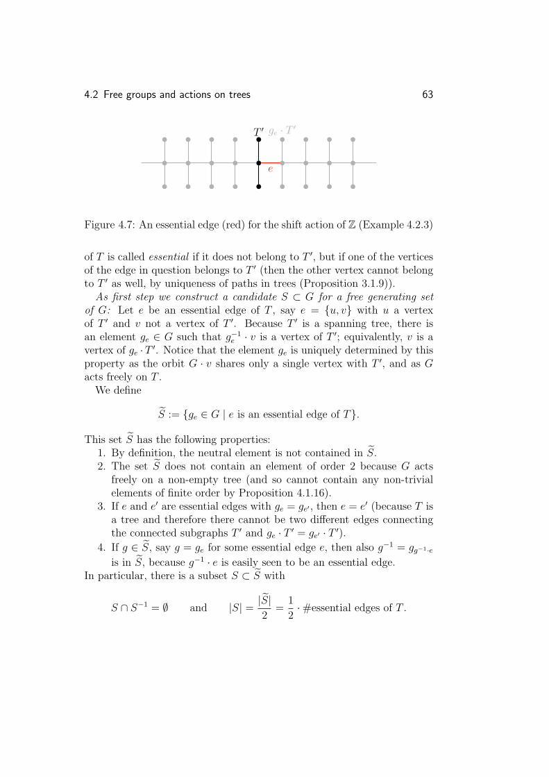
4.2 Free groups and actions on trees 63
e
ge · T ′T ′
Figure 4.7: An essential edge (red) for the shift action of Z (Example 4.2.3)
of T is called essential if it does not belong to T ′, but if one of the verticesof the edge in question belongs to T ′ (then the other vertex cannot belongto T ′ as well, by uniqueness of paths in trees (Proposition 3.1.9)).
As first step we construct a candidate S ⊂ G for a free generating setof G: Let e be an essential edge of T , say e = {u, v} with u a vertexof T ′ and v not a vertex of T ′. Because T ′ is a spanning tree, there isan element ge ∈ G such that g−1
e · v is a vertex of T ′; equivalently, v is avertex of ge · T ′. Notice that the element ge is uniquely determined by thisproperty as the orbit G · v shares only a single vertex with T ′, and as Gacts freely on T .
We define
S := {ge ∈ G | e is an essential edge of T}.
This set S has the following properties:1. By definition, the neutral element is not contained in S.2. The set S does not contain an element of order 2 because G acts
freely on a non-empty tree (and so cannot contain any non-trivialelements of finite order by Proposition 4.1.16).
3. If e and e′ are essential edges with ge = ge′ , then e = e′ (because T isa tree and therefore there cannot be two different edges connectingthe connected subgraphs T ′ and ge · T ′ = ge′ · T ′).
4. If g ∈ S, say g = ge for some essential edge e, then also g−1 = gg−1·e
is in S, because g−1 · e is easily seen to be an essential edge.In particular, there is a subset S ⊂ S with
S ∩ S−1 = ∅ and |S| = |S|2
=1
2·#essential edges of T .

64 4 Groups → geometry, II: Group actions
p
ej
v
T ′
g1 · T ′
gj · T ′
gj+1 · T ′
g · T ′
g · v
Figure 4.8: The set S generates G
The set S (and hence S) generates G: Let g ∈ G. We pick a vertex vof T ′. Because T is connected, there is a path p in T connecting v and g ·v.The path p passes through several copies of T ′, say, g0 ·T ′, . . . , gn ·T ′ of T ′
in this order, where gj+1 6= gj for all j ∈ {0, . . . , n− 1}, and g0 = e, gn = g(Figure 4.8).
Let j ∈ {0, . . . , n− 1}. Because T ′ is a spanning tree and gj 6= gj+1, thecopies gj · T ′ and gj+1 · T ′ are joined by an edge ej. By definition, g−1
j · ej
is an essential edge, and the corresponding group element
sj := g−1j · gj+1
lies in S. Therefore, we obtain that
g = gn = g−10 · gn
= g−10 · g1 · g−1
1 · g2 · · · · · g−1n−1 · gn
= s0 · · · · · sn−1
is in the subgroup of G generated by S. In other words, S is a generatingset of G. (And we can view the graph obtained by collapsing each of the
translates of T ′ in T to a vertex as the Cayley graph Cay(G, S)).
The set S is a free generating set of G: In view of Theorem 3.3.3 it suf-fices to show that the Cayley graph Cay(G,S) does not contain any cycles.Assume for a contradiction that there is an n ∈ N≥3 and a cycle g0, . . . , gn−1
in Cay(G,S) = Cay(G, S). By definition, the elements
∀j∈{0,...,n−2} sj+1 := g−1j · gj+1
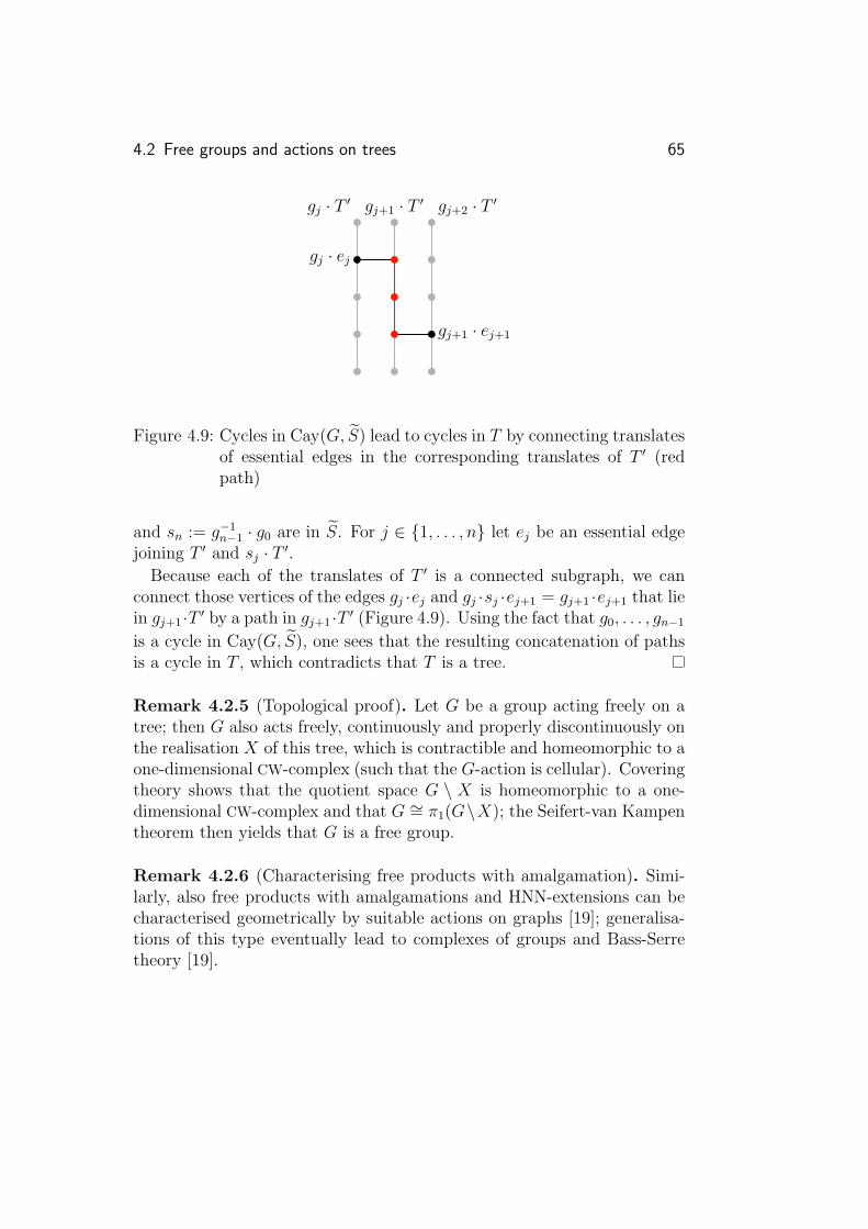
4.2 Free groups and actions on trees 65
gj · T ′ gj+1 · T ′ gj+2 · T ′
gj · ej
gj+1 · ej+1
Figure 4.9: Cycles in Cay(G, S) lead to cycles in T by connecting translatesof essential edges in the corresponding translates of T ′ (redpath)
and sn := g−1n−1 · g0 are in S. For j ∈ {1, . . . , n} let ej be an essential edge
joining T ′ and sj · T ′.Because each of the translates of T ′ is a connected subgraph, we can
connect those vertices of the edges gj ·ej and gj ·sj ·ej+1 = gj+1 ·ej+1 that liein gj+1 ·T ′ by a path in gj+1 ·T ′ (Figure 4.9). Using the fact that g0, . . . , gn−1
is a cycle in Cay(G, S), one sees that the resulting concatenation of pathsis a cycle in T , which contradicts that T is a tree.
Remark 4.2.5 (Topological proof). Let G be a group acting freely on atree; then G also acts freely, continuously and properly discontinuously onthe realisation X of this tree, which is contractible and homeomorphic to aone-dimensional CW-complex (such that the G-action is cellular). Coveringtheory shows that the quotient space G \ X is homeomorphic to a one-dimensional CW-complex and that G ∼= π1(G\X); the Seifert-van Kampentheorem then yields that G is a free group.
Remark 4.2.6 (Characterising free products with amalgamation). Simi-larly, also free products with amalgamations and HNN-extensions can becharacterised geometrically by suitable actions on graphs [19]; generalisa-tions of this type eventually lead to complexes of groups and Bass-Serretheory [19].

66 4 Groups → geometry, II: Group actions
4.3Application: Subgroupsof free groups are free
The characterisation of free groups in terms of free actions on trees allowsus to prove freeness of certain subgroups of suitable groups:
Corollary 4.3.1 (Nielsen-Schreier theorem). Subgroups of free groups arefree.
Proof. Let F be a free group, and let G ⊂ F be a subgroup of F . BecauseF is free, the group F acts freely on a non-empty tree; hence, also the(sub)group G acts freely on this non-empty tree. Therefore, G is a freegroup by Theorem 4.2.1.
Recall that the index of a subgroup H ⊂ G of a group G is the number ofcosets of H in G; we denote the index of H in G by [G : H]. For example,the subgroup 2 · Z of Z has index 2 in Z.
Corollary 4.3.2 (Nielsen-Schreier theorem, quantitative version). Let Fbe a free group of rank n ∈ N, and let G ⊂ F be a subgroup of index k ∈ N.Then G is a free group of rank k · (n− 1) + 1.
In particular, finite index subgroups of free groups of finite rank arefinitely generated.
Proof. Let S be a free generating set of F , and let T := Cay(F, S); so T isa tree and the left translation action of F on T is free. Therefore, also theleft translation action of the subgroup G on T is free (and so G is free).Looking at the proof of Theorem 4.2.1 shows that the rank of G equalsE/2, where E is the number of essential edges of the action of G on T .
We determine E by a counting argument: Let T ′ be a spanning tree ofthe action of G on T . From [F : G] = k we deduce that T ′ has exactly kvertices. For a vertex v in T we denote by dT (v) the degree of v in T ,i.e., the number of neighbours of v in T . Because T is a regular tree all of

4.3 Application: Subgroups of free groups are free 67
whose vertices have degree 2 · |S| = 2 · n, we obtain (where V (T ′) denotesthe set of vertices of T ′)
2 · n · k =∑
v∈V (T ′)
dT (v).
On the other hand, T ′ is a finite tree with k vertices and so has k−1 edges.Because the edges of T ′ are counted twice when summing up the degreesof the vertices of T ′, we obtain
2 · n · k =∑
v∈V (T ′)
dT (v) = 2 · (k − 1) + E;
in other words, the G-action on T has 2 · (k · (n− 1) + 1) essential edges,as desired.
Remark 4.3.3 (Topological proof of the Nielsen-Schreier theorem). An-other proof of the Nielsen-Schreier theorem can be given via covering the-ory: Let F be a free group of rank n; then F is the fundamental groupof a n-fold bouquet X of circles. If G is a subgroup of F , we can look atthe corresponding covering X −→ X of X. As X can be viewed as a one-dimensional CW-complex, also the covering space X is a one-dimensionalCW-complex. On the other hand, any such space is homotopy equivalentto a bouquet of circles, and hence has free fundamental group. BecauseX −→ X is the covering corresponding to the subgroup G of F , it followsthat G ∼= π1(X) is a free group.
Taking into account that the Euler characteristic of finite CW-complexesis multiplicative with respect to finite coverings, one can also prove thequantitative version of the Nielsen-Schreier theorem via covering theory.
Corollary 4.3.4. If F is a free group of rank at least 2, and n ∈ N, thenthere is a subgroup of G that is free of finite rank at least n.
Proof. Exercise.
Corollary 4.3.5. Finite index subgroups of finitely generated groups arefinitely generated.

68 4 Groups → geometry, II: Group actions
Proof. Let G be a finitely generated group, and let H be a finite indexsubgroup of G. If S is a finite generating set of G, then the universalproperty of the free group F (S) freely generated by S provides us with asurjective homomorphism π : F (S) −→ G. Let H ′ be the preimage of Hunder π; so H ′ is a subgroup of F (S), and a straightforward calculationshows that [F (S) : H ′] ≤ [G : H].
By Corollary 4.3.2, the group H ′ is finitely generated; but then also theimage H = π(H ′) is finitely generated.
We will later see an alternative proof of Corollary 4.3.5 via the Svarc-Milnor lemma.
Corollary 4.3.6 (Subgroups of free products). Let G and H be finitegroups. Then all torsion-free subgroups of the free product G ∗H are freegroups.
Sketch of proof. We construct a tree on which the group G ∗H acts withfinite stabilisers:
Let X be the graph– whose set of vertices is V := {x ·G | x ∈ G∗H}∪{x ·H | x ∈ G∗H}
(where we view the vertices as subsets of G ∗H), and– whose set of vertices is{
{x ·G, x ·H}∣∣ x ∈ G ∗H}
(see Figure 4.10 for the free product Z/2Z ∗ Z/3Z). Using the descriptionof the free product G ∗ H in terms of reduced words (Remark 3.3.8) onecan show that the graph X is a tree.
The free group G∗H acts on the tree X by left translation, given on thevertices by
(G ∗H)× V −→ V
(y, x ·G) 7−→ (y · x) ·G(y, x ·H) 7−→ (y · x) ·H.
What are the stabilisers of this action? Let x ∈ G ∗H, and y ∈ G ∗H.Then y is in the stabiliser of x ·G if and only if
x ·G = y · (x ·G) = (y · x) ·G,

4.4 The ping-pong lemma 69
eZ/2 = aZ/2
bZ/2
b2Z/2
abZ/2
ab2Z/2
eZ/3 = bZ/3 = b2Z/3 aZ/3 = abZ/3 = ab2Z/3
Figure 4.10: The tree for the free product Z/2Z ∗ Z/3Z ∼= 〈a, b | a2, b3〉
which is equivalent to y ∈ x ·G · x−1. Analogously, y is in the stabiliser ofthe vertex x ·H if and only if y ∈ x ·H ·x−1. A similar computation showsthat the stabiliser of an edge {x ·G, x ·H} is x ·G · x−1 ∩ x ·H · x−1 = {e}.
Because G and H are finite, all stabilisers of the above action of G ∗Hon the tree X. Therefore, any torsion-free subgroup of G ∗ H acts freelyon the tree X. Applying Theorem 4.2.1 finishes the proof.
A similar technique as in the previous proof shows that all torsion-freesubgroups of SL(2,Qp) are free [19].
4.4
The ping-pong lemma
The following criterion for freeness via suitable actions is due to Klein [?]:
Theorem 4.4.1 (Ping-pong lemma). Let G be a group, generated by twoelements a and b of infinite order. Suppose there is a G-action on a set X

70 4 Groups → geometry, II: Group actions
B A
a
b
a
b
Figure 4.11: The ping-pong lemma
such that there are non-empty subsets A, B ⊂ X with B not included in Aand such that for all n ∈ Z \ {0} we have
an ·B ⊂ A and bn · A ⊂ B.
Then G is freely generated by {a, b}.Proof. It suffices to find an isomorphism Fred({a, b}) ∼= G that extends theidentity on {a, b}. By the universal property of the free group Fred({a, b})there is a group homomorphism ϕ : Fred({a, b}) −→ G extending the iden-tity on {a, b}. Because G is generated by {a, b}, the homomorphism ϕ issurjective.
Assume for a contradiction that ϕ is not injective; hence, there is areduced word w ∈ Fred({a, b})\{ε} with ϕ(w) = e. Depending on the firstand last letter of w there are four cases:
1. The word w starts and ends with a (non-trivial) power of a, i.e.,we can write w = an0bm1an1 . . . bmkank for some k ∈ N and cer-tain n0, . . . , nk,m1, . . . ,mk ∈ Z \ {0}. Then (ping-pong! – see Fig-ure 4.11)
B = e ·B = ϕ(w) ·B= an0 · bm1 · an1 · · · · · bmk · ank ·B⊂ an0 · bm1 · an1 · · · · · bmk · A ping!
⊂ an0 · bm1 · an1 · · · · · ank−1 ·B pong!
⊂ · · · ...
⊂ an0 ⊂ B
⊂ A,
which contradicts the assumption that B is not contained in A.

4.4 The ping-pong lemma 71
2. The word w starts and ends with non-trivial powers of b. Then awa−1
is a reduced word starting and ending in non-trivial powers of a. So
e = ϕ(a) · e · ϕ(a)−1 = ϕ(a) · ϕ(w) · ϕ(a−1) = ϕ(awa−1),
contradicting what we already proved for the first case.3. The word w starts with a non-trivial power of a and ends with a
non-trivial power of b, say w = anw′bm with n.m ∈ Z \ {0} andw′ a reduced word not starting with a non-trivial power of a andnot ending in a non-trivial power of b. Let r ∈ Z \ {0,−n}. Thenarwa−r = ar+nw′bmar starts and ends with a non-trivial power of aand
e = ϕ(arwa−r),
contradicting what we already proved for the first case.4. The word w starts with a non-trivial power of b and ends with a
non-trivial power of a. Then the inverse of w falls into the third caseand ϕ(w−1) = e, which cannot be.
Therefore, ϕ is injective, and so ϕ : Fred({a, b}) −→ G is an isomorphismextending the identity on {a, b}, as was to be shown.
Remark 4.4.2 (Ping-pong lemma for free products). Similarly, using thedescription of free products in terms of reduced words (Remark 3.3.8), onecan show the following: Let G be a group, let G1 and G2 be two subgroupsof G with |G1| ≥ 3 and |G2| ≥ 2, and suppose that G is generated bythe union G1 ∪ G2. If there is a G-action on a set X such that there arenon-empty subsets X1, X2 ⊂ X with X2 not included in X1 and such that
∀g∈G1\{e} g ·X2 ⊂ X1 and ∀g∈G2\{e} g ·X1 ⊂ X2,
then G ∼= G1 ∗G2.

72 4 Groups → geometry, II: Group actions
4.5Application: Free subgroups
of matrix groups
Using the ping-pong lemma we can establish the freeness of certain matrixgroups.
Example 4.5.1 (Free subgroups of SL(2,Z)). We consider the matri-ces a, b ∈ SL(2,Z) given by
a :=
(1 20 1
)and b :=
(1 02 1
).
We show that the subgroup of SL(2,Z) generated by {a, b} is a free groupof rank 2 (freely generated by {a, b}) via the ping-pong lemma:
The matrix group SL(2,Z) acts on R2 by matrix multiplication. We nowconsider the subsets
A :=
{(xy
)∈ R2
∣∣∣∣ |x| > |y|} and B :=
{(xy
)∈ R2
∣∣∣∣ |x| < |y|}of R2. Then A and B are non-empty and B is not contained in A. More-over, for all n ∈ Z \ {0} and all (x, y) ∈ B we have
an ·(xy
)=
(1 2 · n0 1
)·(xy
)=
(x+ 2 · n · y
y
)and
|x+ 2 · n · y| ≥ |2 · n · y| − |x|≥ 2 · |y| − |x|> 2 · |y| − |y|= |y|;
so an ·B ⊂ A. Similarly, we see that bn ·A ⊂ B for all n ∈ Z\{0}. Thus, wecan apply the ping-pong lemma and deduce that the subgroup of SL(2,Z)generated by {a, b} is freely generated by {a, b}. Notice that it would berather awkward to prove this by hand, using only matrix calculations.
4.5 Application: Free subgroups of matrix groups 73
Further examples are given in de la Harpe’s book [12, Chapter II.B]; inparticular, it can be shown that the group of homeomorphisms R −→ Rcontains a free group of rank 2.

74 4 Groups → geometry, II: Group actions

5 Groups → geometry, III:Quasi-isometry
As explained in the introduction, one of the objectives of geometric grouptheory is to view groups as geometric objects. We now add the metriclayer to the combinatorics given by Cayley graphs:
If G is a group and S is a generating set of G, then the paths on theassociated Cayley graph Cay(G,S) induce a metric onG, the so-called wordmetric with respect to the generating set S; unfortunately, in general, thismetric depends on the chosen generating set.
In order to obtain a notion of distance on a group independent of agiven generating set we pass to large scale geometry. Using the languageof quasi-geometry, we arrive at such a notion for finitely generated groups– the so-called quasi-isometry type, which is one of the central objects ofgeometric group theory.
We start with some generalities on isometries, bilipschitz equivalencesand quasi-isometries. As next step, we specialise to the case of finitelygenerated groups. The key to linking the geometry of groups to actualgeometry is the Svarc-Milnor lemma (Section 5.3). Moreover, we discussGromov’s dynamic criterion for quasi-isometry (Section 5.4) and give anoutlook on geometric properties of groups and quasi-isometry invariants(Section 5.5).

76 5 Groups → geometry, III: Quasi-isometry
5.1Quasi-isometry types of
metric spaces
In the following, we introduce different levels of similarity between met-ric spaces: isometries, bilipschitz equivalences and quasi-isometries. Intu-itively, we want a large scale geometric notion of similarity – i.e., we wantmetric spaces to be equivalent if they seem to be the same when lookedat from far away. A guiding example to keep in mind is that we want thereal line and the integers (with the induced metric from the real line) tobe equivalent.
For the sake of completeness, we recall the definition of a metric space:
Definition 5.1.1 (Metric space). A metric space is a set X together witha map d : X ×X −→ R≥0 satisfying the following conditions:
– For all x, y ∈ X we have d(x, y) = 0 if and only if x = y.– For all x, y ∈ X we have d(x, y) = d(y, x).– For all x, y, z ∈ X the triangle inequality holds:
d(x, z) ≤ d(x, y) + d(y, z).
We start with the strongest type of similarity between metric spaces:
Definition 5.1.2 (Isometry). Let f : X −→ Y be a map between metricspaces (X, dX) and (Y, dY ).
– We say that f is an isometric embedding if
∀x,x′∈X dY
(f(x), f(x′)
)= dX(x, x′).
– The map f is an isometry if it is an isometric embedding and if thereis an isometric embedding g : Y −→ X such that
f ◦ g = idY and g ◦ f = idX .
In other words, an isometry is nothing but a bijective isometric em-bedding.

5.1 Quasi-isometry types of metric spaces 77
– Two metric spaces are isometric if there exists an isometry betweenthem.
Remark 5.1.3. Clearly, every isometric embedding is injective, and everyisometry is a homeomorphism with respect to the topologies induced bythe metrics.
The notion of isometry is very rigid – too rigid for our purposes. Wewant a notion of “similarity” for metric spaces that only reflects the largescale shape of the space, but not the local details. A first step is to relaxthe isometry condition by allowing for a uniform multiplicative error:
Definition 5.1.4 (Bilipschitz equivalence). Let f : X −→ Y be a mapbetween metric spaces (X, dX) and (Y, dY ).
– We say that f is a bilipschitz embedding if there is a constant c ∈ R>0
such that
∀x,x′∈X1
c· dX(x, x′) ≤ dY
(f(x), f(x′)
)≤ c · dX(x, x′).
– The map f is a bilipschitz equivalence if it is a bilipschitz embeddingand if there is a bilipschitz embedding g : Y −→ X such that
f ◦ g = idY and g ◦ f = idX .
In other words, a bilipschitz embedding is nothing but a bijectivebilipschitz embedding.
– Two metric spaces are called bilipschitz equivalent if there exists abilipschitz equivalence between them.
Remark 5.1.5. Clearly, every bilipschitz embedding is injective, and everybilipschitz equivalence is a homeomorphism with respect to the topologiesinduced by the metrics.
Hence, also bilipschitz equivalences preserve the local information; sobilipschitz equivalences still remember too much details for our purposes.As next – and final – step, we allow for a uniform additive error:
Definition 5.1.6 (Quasi-isometry). Let f : X −→ Y be a map betweenmetric spaces (X, dX) and (Y, dY ).

78 5 Groups → geometry, III: Quasi-isometry
−4 −3 −2 −1 0 1 2 3 4R
−4 −3 −2 −1 0 1 2 3 4Z
−4 −2 0 2 42 · Z
Figure 5.1: The metric spaces R, Z, and 2 · Z are quasi-isometric
– The map f is a quasi-isometric embedding if there are constants c ∈R>0 and b ∈ R>0 such that
∀x,x′∈X1
c· dX(x, x′)− b ≤ dY
(f(x), f(x′)
)≤ c · dX(x, x′) + b.
– A map f ′ : X −→ Y has finite distance from f if there is a con-stant c ∈ R≥0 with
∀x,x′∈X dX
(f(x), f(x′)
)≤ c.
– The map f is a quasi-isometry if it is a quasi-isometric embeddingfor which there is a quasi-inverse quasi-isometric embedding, i.e., ifthere is a quasi-isometric embedding g : Y −→ X such that g ◦ f hasfinite distance from idY and f ◦ g has finite distance from idX .
– Two metric spaces X and Y are quasi-isometric if there exists aquasi-isometry X −→ Y ; in this case, we write X ∼QI Y .
Example 5.1.7 (Isometries, bilipschitz equivalences and quasi-isometries).Clearly, every isometry is a bilipschitz equivalence, and every bilipschitzequivalence is a quasi-isometry. In general, the converse does not hold:
We consider R as a metric space with respect to the distance functiongiven by the absolute value of the difference of two numbers; moreover,we consider the subsets Z ⊂ R and 2 · Z ⊂ R with respect to the inducedmetrics (Figure 5.1).
Clearly, the inclusions 2 ·Z ↪→ Z and Z ↪→ R are quasi-isometric embed-dings but no bilipschitz equivalences (as they are not bijective). Moreover,

5.1 Quasi-isometry types of metric spaces 79
the maps
R −→ Zx 7−→ bxc,Z −→ 2 · Z
n 7−→
{n if n ∈ 2 · Z,n+ 1 if n 6∈ 2 · Z
are quasi-isometric embeddings that are quasi-inverse to the inclusions(here, bxc denotes the integral part of x, i.e., the largest integer that isnot larger than x).
The spaces Z and 2 · Z are bilipschitz equivalent (via the map given bymultiplication by 2). However, Z and 2 · Z are not isometric – in Z thereare points having distance 1, whereas in 2 ·Z the minimal distance betweentwo different points is 2.
Finally, because R is uncountable but Z and 2 · Z are countable, themetric space R cannot be isometric or bilipschitz equivalent to Z or 2 · Z.
Caveat 5.1.8. In particular, we see that– quasi-isometries in general are neither injective, nor surjective,– quasi-isometries in general are not continuous at all,– in general there is no isometry at finite distance of any given quasi-
isometry,– in general quasi-isometries do not preserve dimension locally.
Example 5.1.9 (More (non-)quasi-isometric spaces).– All non-empty metric spaces of finite diameter are quasi-isometric;
the diameter of a metric space (X, d) is
diamX := supx,y∈X
d(x, y).
– Conversely, if a space is quasi-isometric to a space of finite diamter,then it has finite diameter as well. So the metric space Z (with themetric induced from R) is not quasi-isometric to a non-empty metricspace of finite diameter.
– The metric spaces R and R2 (with respect to the Euclidean metric)are not quasi-isometric (exercise).
80 5 Groups → geometry, III: Quasi-isometry
Exercise 5.1.10.1. Are the metric spaces Z and N with the metrics induced from the
standard metric on R quasi-isometric?2. Are the metric spaces Z and {n3 | n ∈ Z} with the metrics induced
from the standard metric on R quasi-isometric?
Proposition 5.1.11 (Alternative characterisation of quasi-isometries). Amap f : X −→ Y between metric spaces (X, dX) and (Y, dY ) is a quasi-isometry if and only if it is a quasi-isometric embedding with quasi-denseimage; a map f : X −→ Y is said to have quasi-dense image if there is aconstant c ∈ R>0 such that
∀y∈Y ∃x∈X dY
(f(x), y
)≤ c.
Proof. If f : X −→ Y is a quasi-isometry, then, by definition, there existsa quasi-inverse quasi-isometric embedding g : Y −→ X. Hence, there isa c ∈ R>0 such that
∀y∈Y dY
(f ◦ g(y), y
)≤ c;
in particular, f has quasi-dense image.Conversely, suppose that f : X −→ Y is a quasi-isometric embedding
with quasi-dense image. Using the axiom of choice, we construct a quasi-inverse quasi-isometric embedding:
Because f is a quasi-isometric embedding with quasi-dense image, thereis a constant c ∈ R>0 such that
∀x,x′∈X1
c· dX(x, x′)− c ≤ dY
(f(x), f(x′)
)≤ c · dX(x, x′) + c,
∀y∈Y ∃x∈X dY
(f(x), y
)≤ c.
By the axiom of choice, we can define a map
g : Y −→ X
y 7−→ xy,
where we choose for every y ∈ Y an element xy with dY (f(xy), y) ≤ c.The map g is quasi-inverse to f , because: By construction, for all y ∈ Y
we havedY
(f ◦ g(y), y
)= dY (f(xy), y) ≤ c;

5.1 Quasi-isometry types of metric spaces 81
conversely, for all x ∈ X we obtain (using the fact that f is a quasi-isometric embedding)
dX
(g◦f(x), x
)= dX(xf(x), x) ≤ c·dY
(f(xf(x)), f(x)
)+c2 ≤ c·c+c2 = 2·c2.
So f ◦ g and g ◦ f have finite distance from the respective identity maps.Moreover, g also is a quasi-isometric embedding, because: Let y, y′ ∈ Y .
Then
dX
(g(y), g(y′)
)= dX(xy, xy′)
≤ c · dY
(f(xy), f(xy′)
)+ c2
≤ c ·(dY
(f(xy), y
)+ dY (y, y′) + dY
(f(xy′ , y
′)))
+ c2
≤ c ·(dY (y, y′) + 2 · c
)+ c2
= c · dY (y, y′) + 3 · c2,
and
dX
(g(y), g(y′)
)= dX(xy, xy′)
≥ 1
c· dY
(f(xy), f(xy′)
)− 1
≥ 1
c·(dY (y, y′)− dY
(f(xy), y
)− dY
(f(xy′), y
′))− 1
≥ 1
c· dY (y, y′)− 2 · c
c− 1.
(Clearly, the same argument shows that quasi-inverses of quasi-isometricembeddings are quasi-isometric embeddings).
As quasi-isometries are not bijective in general, some care has to betaken when defining quasi-isometry groups of metric spaces:
Proposition 5.1.12 (Quasi-isometry groups).1. The composition of two quasi-isometric embeddings is a quasi-iso-
metric embedding and the composition of two quasi-isometries is aquasi-isometry.
2. Let (X, d) be a metric space. Let QI(X) be the set of all quasi-isometries of type X −→ X, and let QI(X) := QI(X)/ ∼ be the

82 5 Groups → geometry, III: Quasi-isometry
set of quasi-isometries of X modulo finite distance. Then the com-position
QI(X)×QI(X) −→ QI(X)([f ], [g]
)7−→ [f ◦ g]
is well-defined, and QI(X) is a group with respect to this composition.The group QI(X) is the quasi-isometry group of X.
Proof. Exercise.
The first part also shows that quasi-isometry behaves like an equiva-lence relation on the class of all metric spaces. Moreover, we can define acategory whose objects are metric spaces and whose morphisms are quasi-isometric embeddings modulo finite distance; the automorphism groups inthis category then coincide with the quasi-isometry groups defined above.
Having the notion of a quasi-isometry group of a metric space also allowsto define what an action of a group by quasi-isometries on a metric spaceis – namely, a homomorphism from the group in question to the quasi-isometry group of the given space.
Example 5.1.13 (Quasi-isometry groups).
– Clearly, the quasi-isometry group of a metric space of finite diameteris trivial.
– The quasi-isometry group of Z is huge; for example, it contains themultiplicative group R \ {0} as a subgroup via the injective homo-morphism
R \ {0} −→ QI(Z)
α 7−→[n 7→ bα · nc
]together with many rather large and non-commutative groups [18].
5.2 Quasi-isometry types of groups 83
5.2Quasi-isometry types
of groups
Any generating set of a group yields a metric on the group in question bylooking at the lengths of paths in the corresponding Cayley graph. Thelarge scale geometric notion of quasi-isometry then allows us to associategeometric types to finitely generated groups that do not depend on thechoice of finite generating sets.
Definition 5.2.1 (Metric on a graph). Let G = (V,E) be a connectedgraph. Then the map
V × V −→ R≥0
(v, w) 7−→ min{n ∈ N | there is a path of length n
connecting v and w in G}
is a metric on V , the associated metric on V .
Definition 5.2.2 (Word metric). Let G be a group and let S ⊂ G be agenerating set. The word metric dS on G with respect to S is the metricon G associated with the Cayley graph Cay(G,S). In other words,
dS(g, h) = min{n ∈ N | ∃s1,...,sn∈S∪S−1 g−1 · h = s1 · · · · · sn}
for all g, h ∈ G.
Example 5.2.3 (Word metrics on Z). The word metric on Z correspondingto the generating set {1} coincides with the metric on Z induced fromthe standard metric on R. On the other hand, in the word metric on Zcorresponding to the generating set Z, all group elements have distance 1from every other group element.
In general, word metrics on a given group do depend on the chosen setof generators. However, the difference is neglegible when looking at thegroup from far away:

84 5 Groups → geometry, III: Quasi-isometry
Proposition 5.2.4. Let G be a finitely generated group, and let S and S ′
be two finite generating sets of G.1. Then the identity map idG is a bilipschitz equivalence between (G, dS)
and (G, dS′).2. In particular, any metric space (X, d) that is bilipschitz equivalent
(or quasi-isometric) to (G, dS) is also bilipschitz equivalent (or quasi-isometric respectively) to (G, dS′).
Proof. The second part directly follows from the first part because thecomposition of bilipischitz equivalences is a bilipschitz equivalence, and thecomposition of quasi-isometries is a quasi-isometry (Proposition 5.1.12).
Thus it remains to prove the first part: Because S is finite,
c := maxs∈S∪S−1
dS′(e, s)
is finite. Let g, h ∈ G and let n := dS(g, h). Then we can write g−1 · h =s1 · · · · · sn for certain s1, . . . , sn ∈ S ∪ S−1. Using the triangle inequalityand the fact that the metric dS′ is left-invariant by definition, we obtain
dS′(g, h) = dS′(g, g · s1 · · · · · sn)
≤ dS′(g, g · s1) + dS′(g · s1, g · s1 · s2) + . . .
+ dS′(g · s1 · · · · · sn−1, g · s1 · · · · · sn)
= dS′(e, s1) + dS′(e, s2) + · · ·+ dS′(e, sn)
≤ c · n= c · dS(g, h).
Interchanging the roles of S and S ′ shows that also a similar estimateholds in the other direction and hence that idG : (G, dS) −→ (G, dS′) is abilipschitz equivalence.
This proposition gives a precise meaning to the statement that the Cay-ley graphs of a finitely generated group with respect to different finitegenerating sets seem to be the same when looked at from far away (seeFigure 5.2 for an example for the additive group Z).
For infinite generating sets the first part of the above proposition doesnot hold in general; for example taking Z as a generating set for Z leadsto the space (Z, dZ) of finite diameter, while (Z, d{1}) does not have finitediameter (Example 5.2.3).

5.2 Quasi-isometry types of groups 85
−2 −1 0 1 2−2 −1 0 1 2
Cay(Z, {1}
)Cay
(Z, {2, 3}
)Figure 5.2: Cayley graphs of Z having the same large scale geometry
Definition 5.2.5 (Quasi-isometry type of finitely generated groups). LetG be a finitely generated group.
– The group G is bilipschitz equivalent to a metric space X if for some(and hence all) finite generating set S of G the metric spaces (G, dS)and X are bilipschitz equivalent.
– The group G is quasi-isometric to a metric space X if for some (andhence all) finite generating set S of G the metric spaces (G, dS) andXare quasi-isometric. We write G∼QIX if G andX are quasi-isometric.
Analogously we define when two finitely generated groups are called bilip-schitz equivalent or quasi-isometric.
Example 5.2.6. If n ∈ N, then Zn is quasi-isometric to Euclidean space Rn
because the inclusion Zn ↪→ Rn is a quasi-isometric embedding with quasi-dense image. In this sense, Cayley graphs of Zn (with respect to finitegenerating sets) resemble the geometry of Rn (Figure 5.3).
At this point it might be more natural to consider bilipschitz equivalenceof groups as a good geometric equivalence of finitely generated groups;however, later we will see why considering quasi-isometry types of groupsis more appropriate.
The question of how quasi-isometry and bilipschitz equivalence are re-lated for finitely generated groups leads to interesting problems and usefulapplications. A first step towards an answer is the following:
Exercise 5.2.7 (Quasi-isometry vs. bilipschitz equivalence).1. Show that a bijective quasi-isometry between finitely generated groups
(with respect to the word metric of certain finite generating sets) isa bilipschitz equivalence.

86 5 Groups → geometry, III: Quasi-isometry
Figure 5.3: The Cayley graph Cay(Z2, {(1, 0), (0, 1)}
)resembles the geom-
etry of the Euclidean plane R2
2. Does this also hold in general? I.e., are all bijective quasi-isometriesbetween general metric spaces necessarily bilipschitz equivalences?
However, not all infinite fintely generated groups that are quasi-isometricare bilipschitz equivalent. We will study in Section ?? which quasi-isometricgroups are bilipschitz equivalent; in particular, we will see then under whichconditions free products of quasi-isometric groups lead to quasi-isometricgroups.
5.2.1 First examples
As a simple example, we start with the quasi-isometry classification offinite groups:
Remark 5.2.8 (Properness of word metrics). Let G be a group and letS ⊂ G be a generating set. Then S is finite if and only if the word metric dS
on G is proper in the sense that all balls of finite radius in (G, dS) are finite:
If S is infinite, then the ball of radius 1 around the neutral element of Gcontains |S| elements, which is infinite. Conversely, if S is finite, then everyball B of finite radius n around the neutral element contains only finitelymany elements, because the set (S∪S−1)n is finite and there is a surjectivemap (S ∪ S−1)n −→ B; because the metric dS is invariant under the left

5.2 Quasi-isometry types of groups 87
Cay(Z, {1}) Cay(D∞, {x, y})
−2 −1 0 1 2 e x xyyyx
(0, [0]) (1, [0])
(0, [1]) (1, [1])
e s
t st
Cay(Z× Z/2Z, {(1, [0]), (0, [1])}) Cay(D∞, {s, t})
Figure 5.4: The groups Z, Z× Z/2Z and D∞ are quasi-isometric
translation action of G, it follows that all balls in (G, dS) of finite radiusare finite.
Example 5.2.9 (Quasi-isometry classification of finite groups). A finitelygenerated group is quasi-isometric to a finite group if and only if it is finite:All finite groups lead to metric spaces of finite diameter and so all are quasi-isometric. Conversely, if a group is quasi-isometric to a finite group, thenit has finite diameter with respect to some word metric; because balls offinite radius with respect to word metrics of finite generating sets are finite(Remark 5.2.8), it follows that the group in question has to be finite.
Notice that two finite groups are bilipschitz equivalent if and only if theyhave the same number of elements.
This explains why we drew the class of finite groups as a separate smallspot of the universe of groups (Figure 1.2).
The next step is to look at groups (not) quasi-isometric to Z:
Example 5.2.10 (Some groups quasi-isometric to Z). The groups Z andZ × Z/2Z and D∞ are bilipschitz equivalent and so in particular quasi-isometric (see Figure 5.4):
To this end we consider the following two presentations of the infinitedihedral group D∞ by generators and relations:
〈x, y |x2, y2〉 ∼= D∞ ∼= 〈s, t | t2, tst−1 = s−1〉.
The Cayley graph Cay(D∞, {x, y}) is isomorphic to Cay(Z, {1}); in partic-ular, D∞ and Z are bilipschitz equivalent. On the other hand, the Cayley

88 5 Groups → geometry, III: Quasi-isometry
graph Cay(D∞, s, t) is isomorphic to Cay(Z × Z/2Z, {(1, [0]), (0, [1])}); inparticular, D∞ and Z×Z/2Z are bilipschitz equivalent. Because the wordmetrics on D∞ corresponding to the generating sets {x, y} and {s, t} arebilipschitz equivalent, it follows that also Z and Z × Z/2Z are bilipschitzequivalent.
Exercise 5.2.11 (Groups not quasi-isometric to Z). Let n ∈ N≥2.1. Show that the groups Z and Zn are not quasi-isometric. In particular,
R is not quasi-isometric to Rn with the Euclidean metric (becausethese spaces are quasi-isometric to Z and Zn respectively).
2. Show that the group Z is not quasi-isometric to a free group of rank n.
However, much more is true – the group Z is quasi-isometrically rigid inthe following sense:
Theorem 5.2.12 (Quasi-isometry rigidity of Z). A finitely generated groupis quasi-isometric to Z if and only if it is virtually Z. A group is calledvirtually Z if it contains a finite index subgroup isomorphic to Z.
In other words, the property of being virtually Z is a geometric propertyof groups.
We will give a proof of this result later when we have more tools at hand.
5.3
The Svarc-Milnor lemma
Why should we be interested in understanding how finitely generatedgroups look like up to quasi-isometry? A first answer to this questionis given by the Svarc-Milnor lemma, which is one of the key ingredientslinking the geometry of groups to the geometry of spaces arising naturallyin geometry and topology.
The Svarc-Milnor lemma roughly says that given a “nice” action of agroup on a “nice” metric space, we can already conclude that the group in

5.3 The Svarc-Milnor lemma 89
question is finitely generated and that the group is quasi-isometric to thegiven metric space.
In practice, this result can be applied both ways: If we want to knowmore about the geometry of a group or if we want to know that a givengroup is finitely generated, it suffices to exhibit a nice action of this groupon a suitable space. Conversely, if we want to know more about a met-ric space, it suffices to find a nice action of a suitable well-known group.Therefore, the Svarc-Milnor lemma is also called the “fundamental lemmaof geometric group theory.”
5.3.1 Quasi-geodesics and quasi-geodesic spaces
In order to state the Svarc-Milnor lemma, we have to specify what a “nice”metric space is; in particular, we need that the metric on our space can berealised (up to some uniform error) by paths:
Definition 5.3.1 (Geodesic space). Let (X, d) be a metric space.
– Let L ∈ R≥0. A geodesic of length L in X is an isometric embed-ding γ : [0, L] −→ X, where the interval [0, L] carries the metricinduced from the standard metric on R; the point γ(0) is the startpoint of γ, and γ(L) is the end point of γ.
– The metric space X is called geodesic, if for all x, x′ ∈ X there existsa geodesic in X with start point x and end point x′.
Example 5.3.2 (Geodesic spaces). The following statements are illus-trated in Figure 5.5.
– Let n ∈ N. Geodesics in the Euclidean space Rn are precisely theEuclidean line segments. As any two points in Rn can be joined bya line segment, Euclidean space Rn is geodesic.
– The space R2 \ {0} endowed with the metric induced from the Eu-clidean metric on R2 is not geodesic (exercise).
– The sphere S2 with the standard round metric is a geodesic metricspace.
– The hyperbolic plane H2 is a geodesic metric space.

90 5 Groups → geometry, III: Quasi-isometry
R2 S2 H2
Figure 5.5: Geodesic spaces (and example geodesics (red))
Caveat 5.3.3. The notion of geodesic in differential geometry is related tothe one above, but not quite the same; geodesics in differential geometryare only required to be locally isometric, not necessarily globally.
Finitely generated groups together with a word metric coming from afinite generating system are not geodesic (if the group in question is non-trivial), as the underlying metric space is discrete. However, they aregeodesic in the sense of large scale geometry:
Definition 5.3.4 (Quasi-geodesic). Let (X, d) be a metric space and letc, b ∈ R≥0.
– Then a (c, b)-quasi-geodesic in X is a (c, b)-quasi-isometric embed-ding γ : I −→ R, where I = [t, t′] ⊂ R is some closed interval; thepoint γ(t) is the start point of γ, and γ(t′) is the end point of γ.
– The space X is (c, b)-quasi-geodesic, if for all x, x′ ∈ X there existsa (c, b)-quasi-geodesic in X with start point x and end point x′.
Clearly, any geodesic space is also quasi-geodesic (namely, (1, 0)-quasi-geodesic); the converse does not hold in general:
Example 5.3.5 (Quasi-geodesic spaces).– If G = (V,E) is a connected graph, then the associated metric on V
turns V into a (1, 1)-geodesic space because: The distance betweentwo vertices is realised as the length of some path in the graph G,and any path in the graph G that realises the distance between twovertices is a (1, 1)-quasi-geodesic.
– In particular: If G is a group and S is a generating set of G, then(G, dS) is a (1, 1)-quasi-geodesic space.
– For every ε ∈ R>0 the space R2 \ {0} is (1, ε)-quasi-geodesic withrespect to the metric induced from the Euclidean metric on R2 (ex-ercise).
5.3 The Svarc-Milnor lemma 91
5.3.2 The Svarc-Milnor lemma
We now come to the Svarc-Milnor lemma. We start with a formulationusing the language of quasi-geometry; in a second step, we deduce thetopological version, the version usually used in applications.
Proposition 5.3.6 (Svarc-Milnor lemma). Let G be a group, and let Gact on a (non-empty) metric space (X, d) by isometries. Suppose that thereare constants c, b ∈ R>0 such that X is (c, b)-quasi-geodesic and supposethat there is a subset B ⊂ X with the following properties:
– The diameter of B is finite.– The G-translates of B cover all of X, i.e.,
⋃g∈G g ·B = X.
– The set S := {g ∈ G | g ·B′ ∩B′ 6= ∅} is finite, where
B′ := B2·b(B) = {x ∈ X | ∃y∈B d(x, y) ≤ 2 · b}.
Then the following holds:1. The group G is generated by S; in particular, G is finitely generated.2. For all x ∈ X the associated map
G −→ X
g 7−→ g · x
is a quasi-isometry (with respect to the word metric dS on G).
Proof. The set S generates G: Let g ∈ G. We show that g ∈ 〈S〉G byusing a suitable quasi-geodesic and following translates of B along thisquasi-geodesic (Figure 5.6): Let x ∈ B. As X is (c, b)-quasi-geodesic,there is a (c, b)-quasi-geodesic γ : [0, L] −→ X starting in x and endingin g · x. We now look at close enough points on this quasi-geodesic:
Let n := dc · L/be. For j ∈ {0, . . . , n} we define
tj := j · bc,
and tn := L, as well asxj := γ(tj);

92 5 Groups → geometry, III: Quasi-isometry
B
gj−1 ·B′
gj−1 ·B
gj ·B
g ·Bγ
x g · xxj−1
xj
Figure 5.6: Covering a quasi-geodesic by translates of B
notice that x0 = γ(0) = x and xn = γ(L) = g · x. Because the translatesof B cover all of X, there are group elements gj ∈ G with xj ∈ gj · B; inparticular, we can choose g0 := e and gn := g.
For all j ∈ {1, . . . , n}, the group element sj := g−1j−1 · gj lies in S because:
As γ is a (c, b)-quasi-geodesic, we obtain
d(xj−1, xj) ≤ c · |tj−1 − tj|+ b ≤ c · bc
+ b ≤ 2 · b.
Therefore, xj ∈ B2·b(gj−1 · B) = gj−1 · B2·b(B) = gj−1 · B′ (notice that inthe second to last equality we used that G acts on X by isometries). Onthe other hand, xj ∈ gj ·B ⊂ gj ·B′ and thus
gj−1 ·B′ ∩ gj ·B′ 6= ∅;
so, by definition of S, it follows that g−1j−1 · gj ∈ S.
In particular,
g = gn = gn−1 · g−1n−1 · gn = · · · = g0 · s1 · · · · · sn = s1 · · · · · sn
lies in the subgroup generated by S, as desired.The group G is quasi-isometric to X: Let x ∈ X. We show that the
map
ϕ : G −→ X
g 7−→ g · x

5.3 The Svarc-Milnor lemma 93
is a quasi-isometry by showing that it is a quasi-isometric embedding withquasi-dense image. First notice that because G acts by isometries on Xand because the G-translates of B cover all of X, we may assume that Bcontains x (so that we are in the same situation as in the first part of theproof).
The map ϕ has quasi-dense image, because: If x′ ∈ X, then there isa g ∈ G with x′ ∈ g ·B. Then g · x ∈ g ·B yields
d(x′, ϕ(g)
)= d(x′, g · x) ≤ diam g ·B = diamB,
which is assumed to be finite. Thus, ϕ has quasi-dense image.The map ϕ is a quasi-isometric embedding, because: Let g ∈ G. We
first give a uniform lower bound of d(ϕ(e), ϕ(g)) in terms of dS(e, g): Letγ : [0, L] −→ X be as above a (c, b)-quasi-geodesic from x to g ·x. Then theargument from the first part of the proof (and the definition of n) showsthat
d(ϕ(e), ϕ(g)
)= d(x, g · x) = d
(γ(0), γ(L)
)≥ 1
c· L− b
≥ 1
c· b · (n− 1)
c− b
=b
c2· n− 1
c2− b
≥ b
c2· dS(e, g)− 1
c2− b.
Conversely, we obtain a uniform upper bound of d(ϕ(e), ϕ(g)) in termsof dS(e, g) as follows: Suppose dS(e, g) = n; so there are s1, . . . , sn ∈S ∪ S−1 = S with g = s1 · · · · · sn. Hence, using the triangle inequality, thefact that G acts isometrically on X, and the fact that sj · B′ ∩ B′ 6= ∅ forall j ∈ {1, . . . , n− 1} (see Figure 5.7) we obtain
d(ϕ(e), ϕ(g)
)= d(x, g · x)≤ d(x, s1 · x) + d(s1 · x, s1 · s2 · x) + · · ·
+ d(s1 · · · · · sn−1 · x, s1 · · · · · sn · x)= d(x, s1 · x) + d(x, s2 · x) + · · ·+ d(x, sn · x)≤ n · 2 · (diamB + 2 · b)= 2 · (diamB + 2 · b) · dS(e, g).

94 5 Groups → geometry, III: Quasi-isometry
x s · x
B
B′
s ·B
s ·B′
Figure 5.7: If s ∈ S, then d(x, s · x) ≤ 2 · (diamB + 2 · b)
(Recall that diamB is assumed to be finite).Because
d(ϕ(g), ϕ(h)
)= d
(ϕ(e), ϕ(g−1 · h)
)and dS(g, h) = dS(e, g−1 · h)
holds for all g, h ∈ G, these bounds show that ϕ is a quasi-isometricembedding.
Notice that the proof of the Svarc-Milnor lemma does only give a quasi-isometry, not a bilipschitz equivalence. Indeed, the translation action of Zon R shows that there is no analogue of the Svarc-Milnor lemma for bilip-schitz equivalence. Therefore, quasi-isometry of finitely generated groupsis in geometric contexts considered to be the more appropriate notion thanbilipschitz equivalence.
In most cases, the following, topological, formulation of the Svarc-Milnorlemma is used:
Corollary 5.3.7 (Svarc-Milnor lemma, topological formulation). Let Gbe a group acting by isometries on a (non-empty) proper geodesic metricspace (X, d). Furthermore suppose that this action is proper and cocompact.Then G is finitely generated, and for all x ∈ X the map
G −→ X
g 7−→ g · x
is a quasi-isometry.
Before deducing this version from the quasi-geometric version, we brieflyrecall the topological notions occuring in the statement:
5.3 The Svarc-Milnor lemma 95
– A metric space is proper if all balls of finite radius are compact withrespect to the topology induced by the metric.Hence, proper metric spaces are locally compact.
– An action G×X −→ X of a group G on a topological space X (e.g.,with the topology coming from a metric on X) is proper if for allcompact sets B ⊂ X the set {g ∈ G | g ·B ∩B 6= ∅} is finite.Example 5.3.8 (Proper actions).
– The translation action of Z on R is proper (with respect to thestandard topology on R).
– More generally, the action by deck transformations of the fun-damental group of a locally compact path-connected topologicalspace on its universal covering is proper [?].
– Clearly, all stabiliser groups of a proper action are finite. Theconverse is not necessarily true: For example, the action of Zon the circle S1 given by rotation around an irrational angle isfree but not proper (because Z is infinite and S1 is compact).
– An action G × X −→ X of a group G on a topological space X iscocompact if the quotient space G \ X with respect to the quotienttopology is compact.Example 5.3.9 (Cocompact actions).
– The translation action of Z on R is cocompact (with respect tothe standard topology on R), because the quotient is homeo-morphic to the circle S1, which is compact.
– More generally, the action by deck transformations of the funda-mental group of a compact path-connected topological space Xon its universal covering is cocompact because the quotient ishomeomorphic to X [?].
– The (horizontal) translation action of Z on R2 is not cocompact(with respect to the standard topology on R2), because the quo-tient is homeomorphic to the infinite cylinder S1 × R, which isnot compact.
Proof. Notice that under the given assumptions the space X is (1, ε)-quasi-geodesic for all ε ∈ R>0. In order to be able to apply the Svarc-Milnorlemma (Proposition 5.3.6), we need to find a suitable subset B ⊂ X.
A topological argument shows that because the action of G on X isproper and cocompact and because X is locally compact there exists a

96 5 Groups → geometry, III: Quasi-isometry
closed subspace B ⊂ X of finite diameter such that π(B) = X (e.g., asuitable finite union of closed balls [?]); here, π : X −→ G \ X is thecanonical projection onto the quotient space. In particular,
⋃g∈G g ·B = X
and
B′ := B2·ε(B)
has finite diameter. BecauseX is proper, the subset B′ is compact; thus theaction of G on X being proper implies that the set {g ∈ G | g ·B′∩B′ 6= ∅}is finite.
Hence, we can apply the Svarc-Milnor lemma.
5.3.3 Applications of the Svarc-Milnor lemma to group
theory, geometry and topology
The Svarc-Milnor lemma has numerous applications to geometry, topologyand group theory; we will give a few basic examples of this type, indicatingthe potential of the Svarc-Milnor lemma:
– Subgroups of finitely generated groups are finitely generated.– (Weakly) commensurable groups are quasi-isometric.– Certain groups are finitely generated (for instance, certain fundamen-
tal groups).– Fundamental groups of nice compact metric spaces are quasi-isometric
to the universal covering space.
As a first application of the Svarc-Milnor lemma, we give another proof ofthe fact that finite index subgroups of finitely generated groups are finitelygenerated:
Corollary 5.3.10. Finite index subgroups of finitely generated groups arefinitely generated and quasi-isometric to the ambient group.
Proof. Let G be a finitely generated group, and let H be a subgroup offinite index. If S is a finite generating set of G, then the left translationaction of H on (G, dS) is an isometric action satisfying the conditions ofthe Svarc-Milnor lemma (Proposition 5.3.6): The space (G, dS) is (1, 1)-quasi-geodesic. Moreover, we let B ⊂ G be a finite set of representatives

5.3 The Svarc-Milnor lemma 97
of H \G (in particular, the diameter of B is finite). Then H ·B = G, andthe set B′ := B2(B) is finite as well, and so the set
{h ∈ H | h ·B′ ∩B′ 6= ∅}
is finite.Therefore, H is finitely generated and the inclusion H ↪→ G is a quasi-
isometry (with respect to any word metrics on H and G coming from finitegenerating sets).
Pursuing this line of thought consequently leads to the notion of (weak)commensurability of groups:
Definition 5.3.11 ((Weak) commensurability).– Two groups G and H are commensurable if they contain finite index
subgroups G′ ⊂ G and H ′ ⊂ H with G′ ∼= H ′.– More generally, two groups G and H are weakly commensurable if
they contain finite index subgroups G′ ⊂ G and H ′ ⊂ H satisfyingthe following condition: There are normal subgroups N of G′ and Mof H ′ respectively such that the quotient groups G′/N and H ′/M areisomorphic.
In fact, both commensurability and weak commensurability are equiva-lence relations on the class of groups (exercise).
Corollary 5.3.12 (Weak commensurability and quasi-isometry). Let G bea group.
1. Let G′ be a finite index subgroup of G. Then G′ is finitely generatedif and only if G is finitely generated. If these groups are finitelygenerated, then G∼QI G
′.2. Let N be a finite normal subgroup. Then G/N is finitely generated
if and only if G is finitely generated. If these groups are finitelygenerated, then G∼QI G/N .
In particular, if G is finitely generated, then any group weakly commensu-rable to G is finitely generated and quasi-isometric to G.
Proof. Ad 1. In view of Corollary 5.3.10, it suffices to show that G isfinitely generated if G′ is; but clearly combining a finite generating setof G′ with a finite set of representatives of the G′-cosets in G yields a finitegenerating set of G.

98 5 Groups → geometry, III: Quasi-isometry
Ad 2. IfG is finitely generated, then so is the quotientG/N ; conversely, ifG/N is finitely generated, then combining lifts with respect to the canonicalprojection G −→ G/N of a finite generating set of G/N with the finiteset N gives a finite generating set of G.
Let G and G/N be finitely generated, and let S be a finite generating setof G/N . Then the (pre-)composition of the left translation action of G/Non (G/N, dS) with the canonical projection G −→ G/N gives an isometricaction of G on G/N that satisfies the conditions of the Svarc-Milnor lemma(Proposition 5.3.6). Therefore, we obtain G∼QI G/N .
Example 5.3.13.– Let n ∈ N≥2. Then the free group of rank 2 contains a free group
of rank n as finite index subgroup, and hence these groups are com-mensurable; in particular, all free groups of finite rank bigger than 1are quasi-isometric.
– The subgroup of SL(2,Z) generated by the two matrices(1 20 1
)and
(1 02 1
)is free of rank 2; moreover, one can show that this subgroup has finiteindex in SL(2,Z) (exercise). Thus, SL(2,Z) is commensurable to afree group of rank 2 and so quasi-isometric to a free group of rank 2(and hence to all free groups of finite rank bigger than 1).
– Later we will find more examples of finitely generated groups thatare not quasi-isometric. Hence, all these examples cannot be weaklycommensurable (which might be rather difficult to check by hand).
– There exist groups that are weakly commensurable but not commen-surable [12].
Caveat 5.3.14. However, not all quasi-isometric groups are commensu-rable. Let F3 be a free group of rank 3, and let F4 be a free group of rank 4.Then the finitely generated groups (F3 × F3) ∗ F3 and (F3 × F3) ∗ F4 arebilipschitz equivalent (and hence quasi-isometric) (Section ??), but usingthe Euler characteristic one can show that these groups cannot be com-mensurable; moreover, because these groups are torsion-free, they also arenot weakly commensurable.
As second topic, we look at applications of the Svarc-Milnor lemma inalgebraic topology/Riemannian geometry via fundamental groups:

5.3 The Svarc-Milnor lemma 99
Corollary 5.3.15 (Fundamental groups and quasi-isometry). Let M be aclosed (i.e., compact and without boundary) connected Riemannian mani-
fold, and let M be its Riemannian universal covering manifold. Then thefundamental group π1(M) is finitely generated and for every x ∈ M , themap
π1(M) −→ M
g 7−→ g · x
given by the action of the fundamental group π1(M) on M via deck trans-
formations is a quasi-isometry. Here, M and M are equipped with themetrics induced from their Riemannian metrics.
Sketch of proof. Standard arguments from Riemannian geometry and topol-ogy show that in this case M is a proper geodesic metric space and that theaction of π1(M) on M is isometric, proper, and cocompact (the quotientbeing the compact space M) [?].
Applying the topological version of the Svarc-Milnor lemma (Corol-lary 5.3.7) finishes the proof.
We give a sample application of this consequence of the Svarc-Milnorlemma to Riemannian geometry:
Definition 5.3.16 (Flat manifold, hyperbolic manifold).
– A Riemannian manifold is called flat if its Riemannian universal cov-ering is isometric to the Euclidean space of the same dimension.
– A Riemannaian manifold is called hyperbolic if its Riemannian uni-versal covering is isometric to the hyperbolic space of the same di-mension.
Example 5.3.17 (Surfaces). Oriented closed connected surfaces are de-termined up to homeomorphism/diffeomorphism by their genus (i.e., thenumber of “handles”, see Figure 5.8) [?].
– The oriented surface of genus 0 is the sphere of dimension 2; it issimply connected, and so coincides with its universal covering space.In particular, no Riemannian metric on S2 is flat or hyperbolic.

100 5 Groups → geometry, III: Quasi-isometry
· · ·
sphere torus higher genus
Figure 5.8: Oriented closed connected surfaces
– The oriented surface of genus 1 is the torus of dimension 2, which hasfundamental group isomorphic to Z2. One can show that the torusadmits a flat Riemannian metric [?].
– Oriented surfaces of genus g ≥ 2 have fundamental group isomorphicto ⟨
a1, . . . , ag, b1, . . . , bg
∣∣∣∣ g∏j=1
[aj, bj]
⟩and one can show that these surfaces admit hyperbolic Riemannianmetrics [?].
Being flat is the same as having vanishing sectional curvature and beinghyperbolic is the same as having constant sectional curvature −1 [?].
Corollary 5.3.18 ((Non-)Existence of flat/hyperbolic structures).
– If M is a closed connected Riemannian n-manifold that is flat, thenits fundamental group π1(M) is quasi-isometric to Euclidean space Rn,and hence to Zn. In other words: If the fundamental group of a closedconnected smooth n-manifold is not quasi-isometric to Rn (or Zn),then this manifold does not admit a flat Riemannian metric.
– If M is a closed connected Riemannian n-manifold that is hyperbolic,then its fundamental group π1(M) is quasi-isometric to the hyper-bolic space Hn. In other words: If the fundamental group of a closedconnected smooth n-manifold is not quasi-isometric to Hn, then thismanifold does not admit a hyperbolic Riemannian metric.
So, classifying finitely generated groups up to quasi-isometry and study-ing the quasi-geometry of finitely generated groups gives insights into ge-ometry and topology of smooth/Riemannian manifolds.

5.4 The dynamic criterion for quasi-isometry 101
5.4The dynamic criterion for
quasi-isometry
The Svarc-Milnor lemma translates an action of a group into a quasi-isometry of the group in question to the metric space acted upon. Similarly,we can also use certain actions to compare two groups with each other:
Definition 5.4.1 (Set-theoretic coupling). Let G and H be groups. Aset-theoretic coupling for G and H is a non-empty set X together with aleft action of G on X and a right action of H on X that commute witheach other (i.e., (g · x) · h = g · (x · h) holds for all x ∈ X and all g ∈ G,h ∈ H) such that X contains a subset K with the following properties:
1. The G- and H-translates of K cover X, i.e. G ·K = X = K ·H.2. The sets
FG := {g ∈ G | g ·K ∩K 6= ∅},FH := {h ∈ H | K · h ∩K 6= ∅}
are finite.3. For each g ∈ G there is a finite subset FH(g) ⊂ H with g · K ⊂K · FH(g), and for each h ∈ H there is a finite subset FG(h) ⊂ Gwith K · h ⊂ FG(h) ·K.
A right action of a group H on a set X is a map X × H −→ H suchthat (x · h) · h′ = x · (h · h′) holds for all x ∈ X and all h, h′ ∈ H. In otherwords, a right action is the same as an antihomomorphism H −→ SX .
Example 5.4.2. Let X be a group and let G ⊂ X and H ⊂ X be sub-groups of finite index. Then the left action
G×X −→ X
(g, x) 7−→ g · x

102 5 Groups → geometry, III: Quasi-isometry
of G on X and the right action
X ×H −→ X
(x, h) 7−→ x · h
ofH onX commute with each other (because multiplication in the groupXis associative). The set X together with these actions is a set-theoreticcoupling – a suitable subset K ⊂ X can for example be obtained by takingthe union of finite sets of representatives for G-cosets in X and H-cosetsin X respectively.
Proposition 5.4.3 (Quasi-isometry and set-theoretic couplings). Let Gand H be two finitely generated groups that admit a set-theoretic coupling.Then G∼QI H.
Proof. Let X be a set-theoretic coupling space for G and H with the cor-responding commuting actions by G and H; in the following, we will usethe notation from Definition 5.4.1. We prove G ∼QI H by writing down acandidate for a quasi-isometry G −→ H and by then verifying that thismap indeed has quasi-dense image and is a quasi-isometric embedding: Letx ∈ K ⊂ X. Using the axiom of choice, we obtain a map f : G −→ Hsatisfying
g−1 · x ∈ K · f(g)−1
for all g ∈ G.Moreover, we will use the following notation: Let S ⊂ G be a finite
generating set of G, and let T ⊂ H be a finite generating set of H. For asubset B ⊂ H, we define
DT (B) := supb∈B
dT (e, b),
and similarly, we define DS(A) for subsets A of G.The map f has quasi-dense image, because: Let h ∈ H. Using G·K = X
we find a g ∈ G with x ·h ∈ g ·K; because the actions of G and H commutewith each other, it follows that g−1 · x ∈ K · h−1. On the other hand, alsog−1 ·x ∈ K ·f(g)−1, by definition of f . In particular, K ·h−1∩K ·f(g)−1 6= ∅,and so h−1 · f(g) ∈ FH . Therefore,
dT
(h, f(g)
)≤ DTFH ,

5.4 The dynamic criterion for quasi-isometry 103
which is finite (the set FH is finite by assumption) and independent of h;hence, f has quasi-dense image.
The map f is a quasi-isometric embedding, because: Notice that the sets
FH(S) :=⋃
s∈S∪S−1
FH(s) and FG(T ) :=⋃
t∈T∪T−1
FG(t)
are finite by assumption. Let g, g′ ∈ G.
– We first give an upper bound of dT (f(g), f(g′)) in terms of dS(g, g′):More precisely, we will show that
dT
(f(g), f(g′)
)≤ DTFH(S) · dS(g, g′) +DTFH .
To this end let n := dS(g, g′). As first step we show that the in-tersection K · f(g)−1 · f(g′) ∩K · FH(S)n is non-empty: On the onehand,
g−1 · x · f(g′) ∈ K · f(g)−1 · f(g′)
by construction of f . On the other hand, because dS(g, g′) = n wecan write g−1 · g′ = s1 · · · · · sn for certain s1, . . . , sn ∈ S ∪ S−1, andthus
g−1 · x · f(g′) = g−1 · g′ · g′−1 · x · f(g′)
∈ g−1 · g′ ·K · f(g′)−1 · f(g′)
= g−1 · g′ ·K= s1 · · · · · sn−1 · sn ·K⊂ s1 · · · · · sn−1 ·K · FH(S)
...
⊂ K · FH(S)n.
In particular, K · f(g)−1 · f(g′) ∩ K · FH(S)n 6= ∅. Notice that inall these computations we used heavily that the actions of G and Hon X commute with each other.Using the definition of FH , we see that
f(g)−1 · f(g′) ∈ FH · FH(S)n;

104 5 Groups → geometry, III: Quasi-isometry
in particular, we obtain (via the triangle inequality)
dT
(f(g), f(g′)
)= dT
(e, f(g)−1 · f(g′)
)≤ DT (FH · FH(S)n)
≤ n ·DTFH(S) +DTFH
= dS(g, g′) ·DTFH(S) +DTFH ,
as desired (the constants DTFH(S) and DTFH are finite because thesets FH(S) and FH are finite by assumption).
– Moreover, there is a lower bound of dT (f(g), f(g′)) in terms of dS(g, g′):Let m := dT (f(g), f(′g)). Using similar arguments as above, one seesthat
g−1 · x · f(g′) ∈ FG(T )m ·K ∩ g−1 · g′ ·K
and hence that this intersection is non-empty. Therefore, we canconclude that
dS(g, g′) ≤ DSFG(T ) · dT
(f(g), f(g′)
)+DSFG,
which gives the desired lower bound.
Remark 5.4.4 (Cocycles). The construction of the map f in the proofabove is an instance of a more general principle associating interesting mapswith actions. Namely, suitable actions lead to so-called cocycles (which isan algebraic object); considering cocycles up to an appropriate equivalencerelation (“being a coboundary”) then gives rise to so-called cohomologygroups. In this way, certain aspects of group actions on a space can betranslated into an algebraic theory.
Moreover, we need not assume that both groups are finitely generatedas being finitely generated is preserved by set-theoretic couplings:
Exercise 5.4.5 (Set-theoretic couplings and finite generation). Let G andH be groups that admit a set-theoretic coupling. Show that if G is finitelygenerated, then so is H.
The converse of Proposition 5.4.3 also holds: whenever two finitely gen-erated groups are quasi-isometric, then there exists a coupling (even atopological coupling) between them:

5.4 The dynamic criterion for quasi-isometry 105
Definition 5.4.6 (Topological coupling). Let G and H be groups. A topo-logical coupling for G and H is a non-empty locally compact space X to-gether with a proper cocompact left action of G on X by homeomorphismsand a proper cocompact right action of H on X by homeomorphisms thatcommute with each other.
Theorem 5.4.7 (Dynamic criterion for quasi-isometry). Let G and H befinitely generated groups. Then the following are equivalent:
1. There is a topological coupling for G and H.2. There is a set-theoretic coupling for G and H.3. The groups G and H are quasi-isometric.
Sketch of proof. Ad “1 =⇒ 2”. Let G and H be finitely generated groupsthat admit a topological coupling, i.e., there is a non-empty locally com-pact space X together with a proper cocompact action from G on the leftand from H on the right such that these two actions commute with eachother. We show that such a topological coupling gives rise to a set-theoreticcoupling:
A standard argument from topology shows that in this situation thereis a compact subset K ⊂ X such that G ·K = X = K · H. Because theactions of G and H on X are proper, the sets
{g ∈ G | g ·K ∩K 6= ∅}, {h ∈ H | K · h ∩K 6= ∅}
are finite; moreover, properness of the actions, compactness of the set Kas well as the locally compactness of X also give us that for every g ∈ Gthere is a finite set FH(g) ⊂ H satisfying g ·K ⊂ K · FH(g), and similarlyfor elements of H. Hence, we obtain a set-theoretic coupling for G and H;in particular, G and H are quasi-isometric by Proposition 5.4.3.
Ad “2 =⇒ 3”. This was proved in Proposition 5.4.3.
Ad “3 =⇒ 1”. Suppose that the finitely generated groups G and H arequasi-isometric. We now sketch how this leads to a topological couplingof G and H:
Let S ⊂ G and T ⊂ H be finite generating sets of G and H respectively.As first step, we show that there is a finite group F and a constant C ∈ R>0
106 5 Groups → geometry, III: Quasi-isometry
such that the set
X :={f : G −→ H × F
∣∣∣ f has C-dense image in H × F , and
∀g,g′∈G1
C· dS(g, g′) ≤ dT×F
(f(g), f(g′)
)≤ C · dS(g, g′)
}is non-empty: Let f : G −→ H be a quasi-isometry. Because f is a quasi-isometry, there is a c ∈ R>0 such that f has c-dense image in H and
∀g,g′∈G1
c· dS(g, g′)− c ≤ dT
(f(g), f(g′)
)≤ c · dS(g, g′) + c.
In particular, if g, g′ ∈ G with f(g) = f(g′), then dS(g, g′) ≤ c2. Let F bea finite group that has more elements than the dS-ball of radius c2 in G(around the neutral element). Then out of f we can construct an injectivequasi-isometry f : G −→ H × F . Let c ∈ R>0 be chosen in such a waythat f is a (c, c)-quasi-isometric embedding with c-dense image. Becausef is injective, then f satisfies a max(2 · c, c2 + c)-bilipschitz estimate (thisfollows as in Exercise 5.2.7 from the fact that any two different elementsof a finitely generated group have distance at least 1 in any word metric).Hence, F and C := max(2 · c, c2 + c) have the desired property that thecorresponding set X is non-empty.
We now consider the following left G-action and right H-action on X:
G×X −→ X
(g, f) 7−→(x 7→ f(g−1 · x)
)H ×X −→ X
(f, h) 7−→(x 7→ f(x) · (h, e)
)Clearly, these two actions commute with each other.
Furthermore, we can equipX with the topology of pointwise convergence(which coincides with the compact-open topology when viewing X as asubspace of all “continuous” functions G −→ H×F ). By the Arzela-Ascolitheorem [?], the spaceX is locally compact with respect to this topology. Astraightforward computation (also using the Arzela-Ascoli theorem) showsthat the actions of G and H on X are proper and cocompact [?].

5.4 The dynamic criterion for quasi-isometry 107
5.4.1 Applications of the dynamic criterion
A topological version of subgroups of finite index are uniform lattices; thedynamic criterion shows that finitely generated uniform lattices in the sameambient locally compact group are quasi-isometric (Corollary 5.4.9).
Definition 5.4.8 (Uniform lattices). Let G be a locally compact topolog-ical group. A uniform (or cocompact) lattice in G is a discrete subgroup Γof G such that the left translation action of Γ on G is cocompact.
Recall that a topological group is a group G that in addition is a topo-logical space such that the composition G×G −→ G in the group and themap G −→ G given by taking inverses are continuous (on G× G we takethe product topology). A subgroup Γ of a topological group G is discreteif there is an open neighbourhood U of the neutral element e in G suchthat U ∩ Γ = {e}.
A topological space X is called locally compact if for every x ∈ X andevery open neighbourhood U ⊂ X of x there exists a compact neighbour-hood K ⊂ X of x with K ⊂ U . For example, a metric space is locallycompact if and only if it is proper.
Corollary 5.4.9 (Uniform lattices and quasi-isometry). Let G be a locallycompact topological group. Then all finitely generated uniform lattices in Gare quasi-isometric.
Proof. Let Γ and Λ be two finitely generated uniform lattices in G. Thenthe left action
Γ×G −→ G
(γ, g) 7−→ γ · g
of Γ on G and the right action
G× Λ −→ G
(g, λ) 7−→ g · λ
of Λ on G are continuous (because G is a topological group) and commutewith each other, and these actions are cocompact and proper. Hence, Γand Λ are quasi-isometric by the dynamic criterion (Theorem 5.4.7).
108 5 Groups → geometry, III: Quasi-isometry
Example 5.4.10 (Uniform lattices).
– Let n ∈ N. Then Zn is a discrete subgroup of the locally compacttopological group Rn, and Zn \Rn is compact (namely, the n-torus);hence, Zn is a uniform lattice in Rn.
– The subgroup Q ⊂ R is not discrete in R.– Because the quotient Z × {0} \ R2 is not compact, Z × {0} is not
a uniform lattice in R2. Notice that the above corollary would nothold in general without requiring that the lattices are uniform: thegroup Z is not quasi-isometric to R2.
– Let HR be the real Heisenberg group, and let H be the Heisenberggroup, i.e.,
HR :=
1 x z
0 1 y0 0 1
∣∣∣∣∣∣ x, y, z ∈ R
, H :=
1 x z
0 1 y0 0 1
∣∣∣∣∣∣ x, y, z ∈ Z
.
Then HR is a locally compact topological group (with respect to thetopology given by convergence of all matrix coefficients), and H is afinitely generated uniform lattice in HR (exercise).So, any finitely generated group that is not quasi-isometric to Hcannot be a uniform lattice in HR; for example, we will see later thatZ3 is not quasi-isometric to H, and that free groups of finite rank arenot quasi-isometric to H.
– The subgroup SL(2,Z) of the matrix group SL(2,R) is discrete andthe quotient SL(2,Z) \ SL(2,R) has finite invariant measure, butthis quotient is not compact; so SL(2,Z) is not a uniform latticein SL(2,R).
– If M is a closed connected Riemannian manifold, then the isometrygroup Isom(M) of the Riemannian universal covering of M is a lo-cally compact topological group (with respect to the compact-opentopology). Because the fundamental group π1(M) acts by isometries
(via deck transformations) on M , we can view π1(M) as a subgroup
of Isom(M). One can show that this subgroup is discrete and cocom-
pact, so that π1(M) is a uniform lattice in Isom(M) [?].

5.5 Preview: Quasi-isometry invariants and geometric properties 109
5.5 Preview:Quasi-isometry invariantsand geometric properties
The central classification problem of geometric group theory is to classifyall finitely generated groups up to quasi-isometry. As we have seen inthe previous sections, knowing that certain groups are not quasi-isometricleads to interesting consequences in group theory, topology, and geometry.
5.5.1 Quasi-isometry invariants
While a complete classification of finitely generated groups up to quasi-isometry is far out of reach, partial results can be obtained. A generalprinciple to obtain partial classification results in many mathematical fieldsis to construct suitable invariants:
Definition 5.5.1 (Quasi-isometry invariants). Let V be a set. A quasi-isometry invariant with values in V is a map I from the class of all finitelygenerated groups to V such that
I(G) = I(H)
holds for all finitely generated groups G and H with G∼QI H.
Proposition 5.5.2 (Using quasi-isometry invariants). Let V be a set, andlet I be a quasi-isometry invariant with values in V , and let G and Hbe finitely generated groups with I(G) 6= I(H). Then G and H are notquasi-isometric.
Proof. Assume for a contradiction that G and H are quasi-isometric. Be-cause I is a quasi-isometry invariant, this implies I(G) = I(H), whichcontradicts the assumption I(G) 6= I(H). Hence, G and H cannot bequasi-isometric.

110 5 Groups → geometry, III: Quasi-isometry
So, the more quasi-isometry invariants we can find, the more finitelygenerated groups we can distinguish up to quasi-isometry.
Caveat 5.5.3. If I is a quasi-isometry invariant of finitely generated groups,and G and H are finitely generated groups with I(G) = I(H), then in gen-eral we cannot deduce that G and H are quasi-isometric, as the exampleof the trivial invariant shows (see below).
Some basic examples of quasi-isometry invariants are the following:
Example 5.5.4 (Quasi-isometry invariants).– The trivial invariant. Let V be a set containing exactly one ele-
ment, and let I be the map associating with every finitely generatedgroup this one element. Then clearly I is a quasi-isometry invariant– however, I does not contain any interesting information.
– Finiteness. Let V := {0, 1}, and let I be the map that sends all finitegroups to 0 and all finitely generated infinite groups to 1. Then I is aquasi-isometry invariant, because a finitely generated group is quasi-isometric to a finite group if and only if it is finite (Example 5.2.9).
– Rank of free groups. Let V := N, and let I be the map from theclass of all finitely generated free groups to V that associates with afinitely generated free group its rank. Then I is not a quasi-isometryinvariant on the class of all finitely generated free groups, becausefree groups of rank 2 and rank 3 are quasi-isometric.
In order to obtain more interesting classification results we need furtherquasi-isometry invariants. In the following chapters, we will, for instance,study the growth of groups, and ends and boundaries of groups (i.e., ge-ometry at infinity).
5.5.2 Geometric properties of groups and rigidity
Moreover, it is common to use the following term:
Definition 5.5.5 (Geometric property of groups). Let P be a property offinitely generated groups (i.e., any finitely generated group either has P ordoes not have P ). We say that P is a geometric property of groups, in case
5.5 Preview: Quasi-isometry invariants and geometric properties 111
the following holds for all finitely generated groups G and H: If G has Pand H is quasi-isometric to G, then also H has P .
Example 5.5.6 (Geometric properties).– Being finite is a geometric property of groups (Example 5.2.9).– Being Abelian is not a geometric property of groups: For example,
the trivial group and the symmetric group S3 are quasi-isometric(because they are both finite), but the trivial group is Abelian andS3 is not Abelian.
Surprisingly, there are many interesting (many of them purely algebraic!)properties of groups that are geometric:
– Being virtually infinite cyclic is a geometric property.– More generally, for every n ∈ N the property of being virtually Zn is
geometric.– Being finitely generated and virtually free is a geometric property.– Being finitely generated and virtually nilpotent is a geometric prop-
erty of groups.– Being finitely presented is a geometric property of groups.
Proving that these properties are geometric is far from easy; some of thetechniques and invariants needed to prove such statements are explainedin later chapters.
That a certain algebraic property of groups turns out to be geometric isan instance of the rigidity phenomenon; so, for example, the fact that beingvirtually infinite cyclic is a geometric property can also be formulated asthe group Z being quasi-isometrically rigid.
Conversely, in the following chapters, we will also study geometricallydefined properties of finitely generated groups such as hyperbolicity andamenability (both of which are geometric properties of groups), and wewill investigate how the geometry of these groups affects their algebraicstructure.

112 5 Groups → geometry, III: Quasi-isometry

6Growth types of groups
The first quasi-isometry invariant we discuss is the growth type. Basically,we measure the “volume”/size of balls in a given finitely generated groupand study the asymptotic behaviour when the radius tends to infinity.
We will start by introducing growth functions for finitely generatedgroups (with respect to finite generating system); while these growth func-tions depend on the chose finite generating set, a straightforward calcula-tion shows that growth functions for different finite generating sets onlydiffer by a small amount, and more generally that growth functions ofquasi-isometric groups are asymptotically equivalent. This leads to thenotion of growth type of a finitely generated group.
The quasi-isometry invariance of the growth type allows us to show formany groups that they are not quasi-isometric.
Surprisingly, having polynomial growth is a rather strong constraint forfinitely generated groups: By a celebrated theorem of Gromov, all finitelygenerated groups of polynomial growth are virtually nilpotent(!). We willbriefly sketch an elementary approach to this theorem due to Kleiner, Tao,and Shalom.

114 6 Growth types of groups
6.1Growth functions
of finitely generated groups
We start by introducing growth functions of groups with respect to finitegenerating sets:
Definition 6.1.1 (Growth function). Let G be a finitely generated groupand let S ⊂ G be a finite generating set of G. Then
βG,S : N −→ Nr 7−→
∣∣BG,Sr (e)
∣∣is the growth function of G with respect to S; here, BG,S
r (e) denotes the(closed) ball of radius r around e with respect to the word metric dS on G.
Notice that this definition makes sense because balls for word metricswith respect to finite generating sets are finite (Remark 5.2.8).
Example 6.1.2 (Growth functions of groups).– The growth function of the additive group Z with respect to the
generating set {1} clearly is given by
βZ,{1} : N −→ Nr 7−→ 2 · r + 1.
On the other hand, the growth function of Z with respect to thegenerating set {2, 3} is given by
βZ,{2,3} : N −→ N
r 7−→
1 if r = 0
5 if r = 1
6 · r + 1 if r > 1
(exercise). So, in general, growth functions of different generatingsets are different.
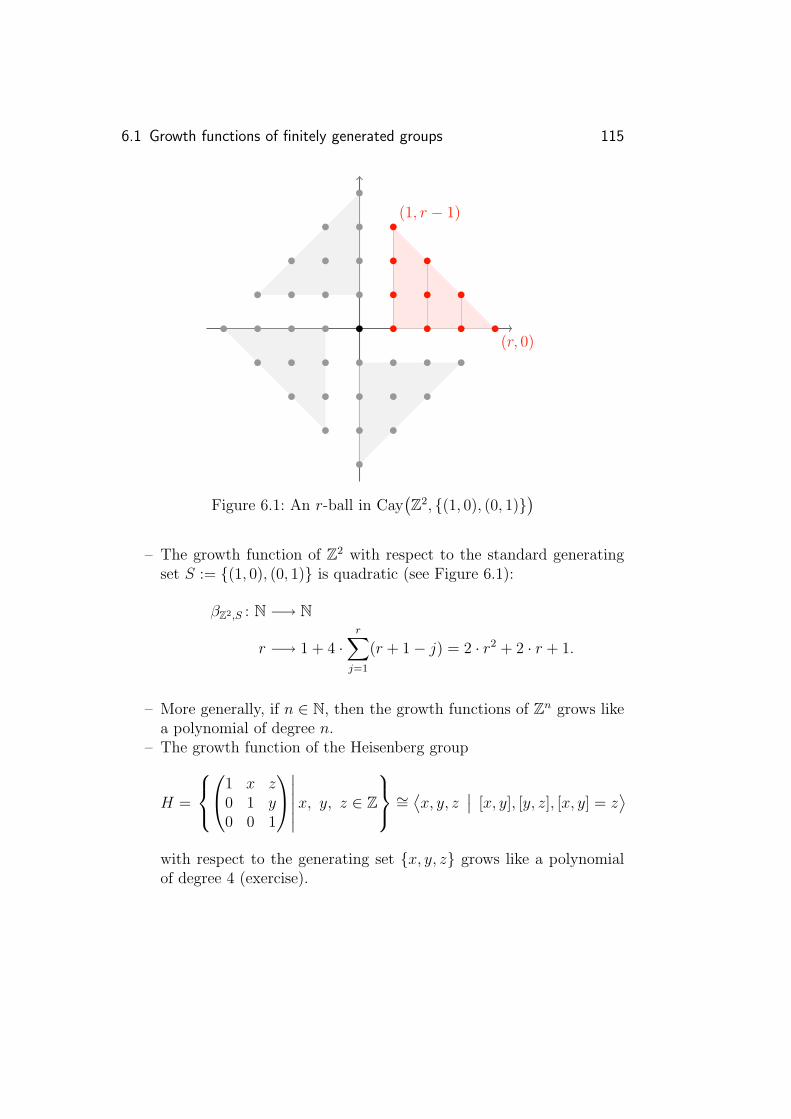
6.1 Growth functions of finitely generated groups 115
(r, 0)
(1, r − 1)
Figure 6.1: An r-ball in Cay(Z2, {(1, 0), (0, 1)}
)– The growth function of Z2 with respect to the standard generating
set S := {(1, 0), (0, 1)} is quadratic (see Figure 6.1):
βZ2,S : N −→ N
r −→ 1 + 4 ·r∑
j=1
(r + 1− j) = 2 · r2 + 2 · r + 1.
– More generally, if n ∈ N, then the growth functions of Zn grows likea polynomial of degree n.
– The growth function of the Heisenberg group
H =
1 x z
0 1 y0 0 1
∣∣∣∣∣∣ x, y, z ∈ Z
∼= ⟨x, y, z
∣∣ [x, y], [y, z], [x, y] = z⟩
with respect to the generating set {x, y, z} grows like a polynomialof degree 4 (exercise).
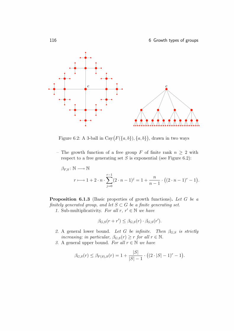
116 6 Growth types of groups
e e
Figure 6.2: A 3-ball in Cay(F ({a, b}), {a, b}
), drawn in two ways
– The growth function of a free group F of finite rank n ≥ 2 withrespect to a free generating set S is exponential (see Figure 6.2):
βF,S : N −→ N
r 7−→ 1 + 2 · n ·r−1∑j=0
(2 · n− 1)j = 1 +n
n− 1·((2 · n− 1)r − 1
).
Proposition 6.1.3 (Basic properties of growth functions). Let G be afinitely generated group, and let S ⊂ G be a finite generating set.
1. Sub-multiplicativity. For all r, r′ ∈ N we have
βG,S(r + r′) ≤ βG,S(r) · βG,S(r′).
2. A general lower bound. Let G be infinite. Then βG,S is strictlyincreasing; in particular, βG,S(r) ≥ r for all r ∈ N.
3. A general upper bound. For all r ∈ N we have
βG,S(r) ≤ βF (S),S(r) = 1 +|S||S| − 1
·((2 · |S| − 1)r − 1
).

6.2 Growth types of groups 117
Proof. Ad 1./2. This follows easily from the definition of the word met-ric dS on G (exercise).
Ad 3. The homomorphism ϕ : F (S) −→ G characterised by ϕ|S = idS iscontracting with respect to the word metrics given by S on F (S) and Grespectively. Moreover, ϕ is surjective. Therefore, we obtain
βG,S(r) =∣∣BG,S
r (e)∣∣ =
∣∣ϕ(BF (S),Sr (e))
∣∣ ≤ ∣∣BF (S),Sr (e)
∣∣ = βF (S),S(r)
for all r ∈ N. The growth function βF (S),S is calculated in Example 6.1.2.
6.2
Growth types of groups
As we have seen, different finite generating sets in general lead to dif-ferent growth functions; however, one might suspect already that growthfunctions coming from different generating sets only differ by some “fi-nite” terms. We therefore introduce the following notion of equivalence forgrowth functions:
6.2.1 Growth types
Definition 6.2.1 (Quasi-equivalence of (generalised) growth functions).– A generalised growth function is a function of type R≥0 −→ R≥0 that
is increasing.– Let f , g : R≥0 −→ R≥0 be generalised growth functions. We say thatg quasi-dominates f , if there exist c, b ∈ R>0 such that
∀r∈R≥0f(r) ≤ c · g(c · r + b) + b.
If g quasi-dominates f , then we write f ≺ g.

118 6 Growth types of groups
– Two generalised growth functions f , g : R≥0 −→ R≥0 are quasi-equivalent if both f ≺ g and g ≺ f ; if f and g are quasi-equivalent,then we write f ∼ g.
A straightforward computation shows that quasi-domination defines apartial order on the set of all generalised growth functions and that quasi-equivalence indeed defines an equivalence relation.
Example 6.2.2 (Generalised growth functions).– Monomials. If a ∈ R≥0, then
R≥0 −→ R≥0
x 7−→ xa
is a generalised growth function.For all a, a′ ∈ R≥0 we have
(x 7→ xa) ≺ (x 7→ xa′)⇐⇒ a ≤ a′,
because: If a ≤ a′, then for all r ∈ R≥0
ra ≤ ra′ + 1,
and so (x 7→ xa) ≺ (x 7→ xa′).Conversely, if a > a′, then for all c, b ∈ R>0 we have
limr→∞
ra
c · (c · r + b)a′=∞;
thus, for all c, b ∈ R>0 there is r ∈ R≥0 such that ra ≥ c·(c·r+b)a′+b,and so (x 7→ xa) 6≺ (x 7→ xa′).In particular, (x 7→ xa) ∼ (a 7→ xa′) if and only if a = a′.
– Exponential functions. If a ∈ R>1, then
R≥0 −→ R≥0
x 7−→ ax
is a generalised growth function. A straightforward calculation showsthat
(x 7→ ax) ∼ (x 7→ a′x)

6.2 Growth types of groups 119
holds for all a, a′ ∈ R>1, as well as
(x 7→ ax) � (x 7→ xa′) and (x 7→ ax) 6≺ (x 7→ xa′)
for all a ∈ R>1 and all a′ ∈ R≥0 (exercise).
Example 6.2.3 (Growth functions yield generalised growth functions).Let G be a finitely generated group, and let S ⊂ G be a finite generatingset. Then the function
R≥0 −→ R≥0
r −→ βG,S(dre)
associated with the growth function βG,S : N −→ N indeed is a generalisedgrowth function (which is also sub-multiplicative).
If G and H are finitely generated groups with finite generating sets Sand T respectively, then we say that the growth function βG,S is quasi-dominated by/quasi-equivalent to the growth function βH,T if the associatedgeneralised growth functions are quasi-dominated by/quasi-equivalent toeach other.
Notice that then βG,S is quasi-dominated by βH,T if and only if thereexist c, b ∈ N such that
∀r∈N βG,S(r) ≤ c · βH,T (c · r + b) + b.
6.2.2 Growth types and quasi-isometry
We will now show that growth functions of different finite generating setsare quasi-equivalent; more generally, we show that the quasi-equivalenceclass of growth functions of finite generating sets is a quasi-isometry in-variant:
Proposition 6.2.4 (Growth functions and quasi-isometry). Let G and Hbe finitely generated groups, and let S ⊂ G and T ⊂ H be finite generatingsets of G and H respectively.
1. If there exists a quasi-isometric embedding (G, dS) −→ (H, dT ), then
βG,S ≺ βH,T .

120 6 Growth types of groups
2. In particular, if G and H are quasi-isometric, then the growth func-tions βG,S and βH,T are quasi-equivalent.
Proof. The second part follows directly from the first one (and the defi-nition of quasi-isometry and quasi-equivalence of generalised growth func-tions).
For the first part, let f : G −→ H be a quasi-isometric embedding; hence,there is a c ∈ R>0 such that
∀g,g′∈G1
c· dS(g, g′)− c ≤ dT
(f(g), f(g′)
)≤ c · dS(g, g′) + c.
We write e′ := f(e), and let r ∈ N. Using the estimates above we obtainthe following:
– If g ∈ BG,Sr (e), then dT (f(g), e′) ≤ c · dS(g, e)+ c ≤ c · r+ c, and thus
f(BG,S
r (e))⊂ BH,T
c·r+c(e′).
– For all g, g′ ∈ G with f(g) = f(g′), we have
dS(g, g′) ≤ c ·(dT (f(g), f(g′)) + c
)= c2.
Because the metric dT on H is invariant under left translation, it followsthat
βG,S(r) ≤∣∣BG,S
c2 (e)∣∣ · ∣∣BH,T
c·r+c(e′)∣∣
=∣∣BG,S
c2 (e)∣∣ · ∣∣BH,T
c·r+c(e)∣∣
= βG,S(c2) · βH,T (c · r + c),
which shows that βG,S ≺ βH,T (the term βG,S(c2) does not depend on theradius r).
In particular, we can define the growth type of finitely generated groups:
Definition 6.2.5 (Growth types of finitely generated groups). Let G bea finitely generated group. The growth type of G is the (common) quasi-equivalence class of all growth functions of G with respect to finite gener-ating sets of G.
6.2 Growth types of groups 121
Corollary 6.2.6 (Quasi-isometry invariance of the growth type). By Propo-sition 6.2.4, the growth type of finitely generated groups is a quasi-isometryinvariant, i.e., quasi-isometric finitely generated groups have the samegrowth type.
In other words: Finitely generated groups having different growth typescannot be quasi-isometric.
Example 6.2.7 (Growth types).– If n ∈ N, then Zn has the growth type of (x 7→ xn).– The Heisenberg group has the growth type of (x 7→ x4).– Non-Abelian free groups of finite rank have the growth type of the
exponential function (x 7→ ex).
In other words: The groups Zn and the Heisenberg group have polyno-mial growth, while non-Abelian free groups have exponential growth:
Definition 6.2.8 (Exponential growth, polynomial growth, intermediategrowth). Let G be a finitely generated group.
– The group G is of exponential growth, if it has the growth type of theexponential map (x 7→ ex).
– The group G has polynomial growth, if for one (and hence any) finitegenerating set S of G there is an a ∈ R>0 such that βG,S ≺ (x 7→ xa).
– The group G is of intermediate growth, if it is neither of exponentialnor of polynomial growth.
Recall that growth functions of finitely generated groups grow at mostexponentially (Proposition 6.1.3), and that polynomials and exponentialfunctions are not quasi-equivalent; hence the term “intermediate growth”does make sense and a group cannot have exponential and polynomialgrowth at the same time.
Moreover, it follows from Proposition 6.2.4 and Example 6.2.2 that hav-ing exponential growth/polynomial growth/intermediate growth respec-tively is a geometric property of groups.
Example 6.2.9 (Distinguishing quasi-isometry types of basic groups).– We can recover the rank of free Abelian groups from their quasi-
isometry type, namely: For all m, n ∈ N we have
Zm ∼QI Zn ⇐⇒ m = n;

122 6 Growth types of groups
this follows by combining Example 6.2.2, Example 6.2.7, and theabove corollary.
– Similarly, we obtain for the Heisenberg group H that H 6∼QIZ3, whichmight be surprising because H fits into a short exact sequence
1 −→ Z −→ H −→ Z2 −→ 1
of groups!– Let F be a non-Abelian free group of finite rank, and let n ∈ N.
Because F grows exponentially, but Zn has polynomial growth, weobtain
F 6∼QI Zn.
Corollary 6.2.10 (Growth of subgroups). Let G be a finitely generatedgroup, and let H be a finitely generated subgroup of G. If T is a finitegenerating set of H, and S is a finite generating set of G, then
βH,T ≺ βG,S.
Proof. Let S ′ := S ∪ T ; then S ′ is a finite generating set of G. Let r ∈ N;then for all h ∈ BH,T
r (e) we have
dS′(h, e) ≤ dT (h, e) ≤ r,
and so BH,Tr (e) ⊂ BG,S
r (e). In particular,
βH,T (r) ≤ βG,S′(r),
and thus βH,T ≺ βG,S′ . Moreover, we know that (G, dS) and (G, dS′) arequasi-isometric, and hence the growth functions βG,S′ and βG,S are quasi-equivalent by Proposition 6.2.4. Therefore, we obtain βH,T ≺ βG,S, asdesired.
Example 6.2.11 (Subgroups of exponential growth). Let G be a finitelygenerated group; if G contains a non-Abelian free subgroup, then G hasexponential growth. For instance, it follows that the Heisenberg groupdoes not contain a non-Abelian free subgroup.
Grigorchuk was the first to show that there indeed exist groups that haveintermediate growth [?, 12]:
6.2 Growth types of groups 123
Theorem 6.2.12 (Existence of groups of intermediate growth). Thereexists a finitely generated group of intermediate growth.
This group constructed by Grigorchuk can be described via automor-phisms of trees or as a so-called automatic group.
Furthermore, the group constructed by Grigorchuk also has several otherinteresting properties [12, Chapter VIII]; for example, it is a finitely gener-ated infinite torsion group, and it is commensurable to the direct productwith itself.

124 6 Growth types of groups

Bibliography
[1] Martin Aigner. Diskrete Mathematik, fifth edition, Vieweg Verlag,2004. Cited on page: 58
[2] Margaret A. Armstrong. Groups and Symmetry, Undergraduate Textsin Mathematics, Springer, 1988. Cited on page: 49, 58
[3] Tim Austin. Rational group ring elements with kernelshaving irrational dimension, preprint, available online atarXiv:0909.2360 [math.GR], 2009. Cited on page: 27
[4] Gilbert Baumslag. Wreath products and finitely presented groups,Math. Z., 75, pp. 22–28, 1961. Cited on page: 25
[5] Martin R. Bridson. Non-positive curvature and complexity for finitelypresented groups, volume 2 of International Congress of Mathemati-cians, pp. 961–987, EMS, 2006. Cited on page: 2, 3, 5
[6] Martin R. Bridson. Geometric and combinatorial group theory, in ThePrinceton Companion to Mathematics, pp. 431–448, Princeton Univer-sity Press, 2008. Cited on page: 5
[7] Martin R. Bridson, Andre Haefliger. Metric Spaces of Non-positiveCurvature, Band 319 der Grundlehren der Mathematischen Wis-senschaften, Springer, 1999. Cited on page: 5, 41

126 Bibliography
[8] Kenneth S. Brown. Cohomology of Groups, volume 87 of GraduateTexts in Mathematics, Springer, 1982. Cited on page: 30, 42
[9] Thomas H. Cormen, Charles E. Leiserson, Ronald L. Rivest, Clif-ford Stein. Introduction to algorithms, third edition. MIT Press, 2009.Cited on page: 35
[10] Reinhard Diestel. Graph theory, third edition, volume 173 of GraduateTexts in Mathematics, Springer, 2005. Cited on page: 35
[11] Misha Gromov. Hyperbolic groups. in Essays in group theory, vol-ume 8 of Math. Sci. Res. Inst. Publ., pp. 75–263, Springer, 1987.Cited on page: 5
[12] Pierre de la Harpe. Topics in Geometric Group Theory, Chicago Uni-versity Press, 2000. Cited on page: 5, 26, 73, 98, 122, 123
[13] John M. Harris, Jeffrey L. Hirst, Michael J. Mossinghoff. Combi-natorics and Graph Theory, second edition, Undergraduate Texts inMathematics, Springer, 2008. Cited on page: 35
[14] Serge Lang. Algebra, Revised third edition. Volume 211 of GraduateTexts in Mathematics, Springer, 2002. Cited on page: 8
[15] John M. Lee. Riemannian Manifolds. An Introduction to Curvature.Volume 176 of Graduate Texts in Mathematics, Springer, 1997. Citedon page: 5
[16] Clara Loh. Group Cohomology and Bounded Cohomol-ogy. An Introduction for Topologists. Lecture notes,2010. Available online at http://www.mathematik.uni-regensburg.de/loeh/teachin/topologie3 ws0910 Cited on page: 30,42
[17] William S. Massey. A Basic Course in Algebraic Topology. Volume 127of Graduate Texts in Mathematics, Springer, 1991. Cited on page: 32
[18] Parameswaran Sankaran. On homeomorphisms and quasi-isometriesof the real line, Proc. Amer. Math. Soc., 134, no. 7, pp. 1875–1880,2006. Cited on page: 82

Bibliography 127
[19] Jean-Pierre Serre. Trees, corrected 2nd printing of the 1980 Englishtranslation, Springer Monographs in Mathematics, Springer, 2003.Cited on page: 5, 45, 65, 69
[20] John R. Stallings. On torsion-free groups with infinitely many ends,Annals of Mathematics, 88, pp. 312–334, 1968. Cited on page: 34