math 697: introduction to geometric group theoryzhufeng/math697_ggt.pdf · math 697: introduction...
TRANSCRIPT

Math 697: Introduction to Geometric Group Theory
Notes from course given by Dick Canary, Fall 2014.
August 23, 2016
0 Overview
0.1 A Rambling
Geometric group theory is really “a collection of things put together by a state of mind.” These things defi-nitely include hyperbolic group theory, but also various other things such as CAT(0) groups, topologicalgroup theory, and so on ...
A little more concretely, geometric group theory is the study of groups by looking at their actions onspaces.
Given a [finitely-presented] group G = 〈x1, . . . , xn | r1, . . . , rm〉, we can define the word metric distanceby setting d(g, h) to be the minimal length of word in x1, . . . , xn (and their inverses) over all representationsof g−1h. We define the Cayley graph ΓG of G by taking the vertices to be the elements of G and drawingedges labelled xi joining each g to gxi
Example 0.1. • If G = Z = 〈a |〉, then ΓG is a line (∼= R.)
a a a a
a−2 a−1 1 a a2· · · · · ·
• If G = Z2 = 〈a, b | [a.b]〉, then ΓG is a 2-dimensional lattice (“what is this? It is graph paper.”)
0 a
b
ab
= ba
• If G = F2 = 〈a, b |〉, then ΓG is an infinite 4-valent tree (the universal cover of S1 ∨ S1)—see below
If M is a compact manifold, then π1(M) acts properly discontinuously and co-compactly on M .
Example 0.2. If M = T 2, then π1(M) = Z2, which acts properly discontinuously and cocompactly onM = R2; we note that R2 “looks like” Z2 (coarsely speaking.)
If M is a compact 3-manifold (e.g. a solid genus-2 torus), M is a thickening of ΓF2, the infinite 4-valent
tree.
We make precise the notion of “looks like” by using the notion of quasi-isometry.Note that our spaces X and Y are usually assumed to be proper (i.e. closed balls are compact) and
geodesic (i.e. distance between two points is given by the length of a shortest path.)
1

a a a a
b−1
b
b−1
b−1
a−1 a
b
baa−1
b−1
b−1
b−1
a−1 a
a−1a−1 b
b−1
a a
b−1
b
b
b
baa−1
a a
b−1
ba−1a−1 b
b−1
b−1
b−1
b−1
b−1
a−1 a
a−1a−1 b
b−1
a a
b−1
b
a−1a−1a−1 b
b−1
b
baa−1
b−1
b−1
a−1 a
a a a
b−1
b
b−1
b−1
a−1 a
b
baa−1
b
b
b
baa−1
a a
b−1
ba−1a−1 b
b−1
a a a
b−1
b
b−1
b−1
a−1 a
b
baa−1
a−1a−1a−1 b
b−1
b
baa−1
b−1
b−1
a−1 a
a−1a−1a−1a−1 b
b−1
b
baa−1
b−1
b−1
a−1 a
b
b
baa−1
a a
b−1
ba−1a−1 b
b−1
b−1
b−1
b−1
a−1 a
a−1a−1 b
b−1
a a
b−1
b
Figure 1: Part of a Cayley graph of a nonabelian free group
Definition 0.3. h : X → Y is a quasi-isometric embedding if there exist k, c s.t. 1kd(x, z) − c ≤
d (h(x), h(z)) ≤ kd(x, z) + c for all x, z ∈ X.h is a quasi-isometry if in addition it is “coarsely surjective”, i.e. there exists D ≥ 0 s.t. for all y ∈ Y ,
there exists x ∈ X s.t. d(h(x), y) ≤ D.1
A key result in geometric group theory is the Milnor-Svarc lemma, which states that if G acts properlydiscontinuously and co-compactly on a space X, then X is quasi-isometric to G with the word metric.
Note that this notion of quasi-isometry, though seemingly loose and geometric, can capture algebraicaspects of structure (or aspects of algebraic structure.) e.g. G quasi-isometric to a free group implies Gvirtually free.2 There is also Gromov’s theorem, which states that any group with polynomial growth isvirtually nilpotent.
In fact, we can also use algebra to clarify geometry, as in the following [re-]formulation of hyperbolic
1Think of the plane, and graph paper.2“Virtually” or “almost” in this context means true up to (true for a) finite-index subgroup. These adjectives will appear a
lot, because quasi-isometry fails to distinguish between the whole group and finite-index subgroups.
2
spaces by Gromov:
Fact. Suppose X is simply-connected with (sectional) curvature ≤ −k < 0. Then there exists δ = δ(k) suchthat any geodesic triangle in X is δ-slim, meaning that if T has vertices x, y, z, then [x, z] ⊂ Nδ([x, y]∪[y, z]),i.e. ∀t ∈ [x, z] : ∃s ∈ [x, y] ∪ [y, z] s.t. d(s, t) < δ.
Definition 0.4 (Gromov, possibly Alexander). X is δ-hyperbolic if every geodesic triangle in X is δ-slim.e.g. trees are 0-hyperbolic.
A space is hyperbolic if it is δ-hyperbolic for some δ ≥ 0.A group is hyperbolic if it acts properly discontinuously and co-compactly on a hyperbolic space.
Hyperbolic groups have some very nice properties:
• Hyperbolic groups have solvable word problem (which we might formulate as “can I build the Cayleygraph [algorithmically]?”) by Dehn’s algorithm.
• They also have solvable conjugacy problem and isomorphism problem.3
• The Tits Alternative: if a hyperbolic group G is not virtually cyclic, it contains a F2.
• A hyperbolic group cannot contain a copy of Z2.
• A hyperbolic group has only finitely many conjugacy classzes of finite subgroups.
• Being a hyperbolic space / group is a condition invariant under quasi-isometry.
Hyperbolic spaces are those with constant negative curvature (-1); we can generalize this notion to lookat spaces X with constant non-positive curvature, and this brings us to the theory of CAT(0) groups:
Definition 0.5. A simply-connected space X is CAT(0) if every geodesic triangle in X is at least as thinas a Euclidean triangle with the same edge lengths.
G is CAT(0) if it acts properly and cocompactly on a CAT(0) space.
Definition 0.6. CAT(0) cube complexes are formed by gluing Euclidean unit cubes along faces.e.g. R2 is a CAT(0) cube complex
Example 0.7. Right-Angled Artin Groups (RAAGs) are CAT(0) groups AΓ formed as follows: start witha finite graph Γ; define
AΓ = 〈Γ(0) | vw = wv ⇐⇒ (v, w) ⊂ Γ(1)〉
i.e. the elements of AΓ are the vertices of Γ, and we add a commutator relation between two elements iffthere is an edge between the corresponding vertices.
e.g. if Γ is the empty graph on n vertices, then AΓ = Fn.If Γ = Kn, then AΓ = Zn.If Γ consists of two disjoint edges on 4 vertices, then AΓ = Z2 ∗ Z2.These groups are “interpolating between the free group and the free abelian group.”
Theorem 0.8 (Agol, Wise). If a hyperbolic group G acts properly discontinuously and cocompactly on aCAT(0) cube complex (in this case we say G is a cubulation), then a finite-index subgroup of G embeds ina RAAG.
Theorem 0.9 (Haglund-Wise, Kahn-Markovic). If M is a closed hyperbolic 3-manifold, then M is cubulated.
Finally, there is topological group theory. The prototypical result here is the proposition that statesthat every subgroup of a free group is free, proven using covering spaces. There is also the followinggeneralisation of this:
Theorem 0.10 (Kurosh). If G = G1 ∗G2 and H ⊂ G, then H = F ∗λ∈Λ Hλ, where F is free, and each HΛ
is conjugate to a a subgroup of G1 or G2.(See Figure 2.)
3Something involving Tietze transformations was name-dropped here.
3

Figure 2: A free product may be thought of as the fundamental group of a wedge of spaces.
This has the following corollary:
Corollary. If G is finitely-generated, then G has a unique free decomposition G = G1 ∗ · · · ∗Gn where eachGi is freely indecomposable (i.e. does not split as a free product.)
Other topics that might come under this last heading include JSJ decompositions and Bass-Serre theory.
0.2 Definitions and quasi-isometry
Definition 0.11. Given X a metric space and α : [0, 1]→ X a path,
`X(α) := sup0=t0<t1<···<tn=1
n−1∑i=0
d(α(ti), α(ti+1))
Definition 0.12. α is rectifiable if `X(α) <∞.
Definition 0.13. α is geodesic if `X(α) = d(α(0), α(1)).
Exercise. (1) A subpath of a geodesic is a geodesic,
(2) If 0 ≤ s ≤ t ≤ u ≤ 1, then
d(α(s), α(t)) + d(α(t), α(u)) = d(α(s), α(u))
if α is a geodesic.
Definition 0.14. A metric space is geodesic if any two points are joined by a (by some) geodesic.e.g. Cayley graphs, Riemannian manifolds, curve complexes, etc.
Definition 0.15. X is proper if all closed metric balls are compact.
Our spaces will be proper geodesic metric spaces (mostly.)We always assume that G acts by isometries on X, i.e. d(x, y) = d(s(x), s(y) for all x, y ∈ X and
s ∈ G. This is a common (and apparently commonly unstated!) assumption in geometric group theory.
Definition 0.16. An action is properly discontinuous (or proper) if whenever K is compact g ∈ G |g(K) ∩K 6= ∅ is finite.
Definition 0.17. An action of G is co-compact if X/G is compact.
Remark. X/G is a metric space, with the metric given by dX/G([x], [y]) := dX(Gx,Gy).
Hence X/G compact =⇒ ∃R s.t. G(BR(x0)) = X—we can take e.g. R = diam(X/G).
Fact. If G acts properly and co-compactly on a geodesic proper metric space, then G is finitely generated.
Proof. Choose D = B2 diam(X/G)(x), U = int(D). Note U ⊃ Bdiam(X/G)(x). Then G(U) = X.Let S = g ∈ G | g(D) ∩D 6= ∅. S is finite.
Claim. S is a generating set.Let H = 〈S〉 ⊂ G. If H 6= G, then let V = Hu and W = (G \H)u: V and W are non-empty and open,
and X is connected (since path-connected, since geodesic), so V ∩W 6= ∅.Let x ∈ V ∩W . x ∈ V =⇒ ∃h ∈ H, p ∈ U s.t. h(p) = x. x ∈ W =⇒ ∃g ∈ G \H, q ∈ U s.t. g(q) = x.
Then hg−1(p) = q and so hg−1 ∈ S, which implies g ∈ H. Contradiction.
4

Recall that h : X → Y is a (k, c)-quasi-isometric embedding if ∀x, z ∈ X
a
kd(x, z)− c ≤ d(h(x), h(z)) ≤ kd(x, z) + c
(k is a bi-Lipschitz constant, disregard scale ≤ c.)
Fact. If h : X → Y is a quasi-isometry, then ∃ quasi-isometry j : X → Y s.t. d(j(h(x)), x), d(h(j(y)), y) ≤ Rfor all x ∈ X, y ∈ Y , and some R ∈ R+
0 .j is called a quasi-inverse.
Proof. If y ∈ Y , then ∃x ∈ X s.t. d(y, h(x)) ≤ C. Choose j(y) s.t. d(y, h(j(y)) ≤ C. Then
d(j(y), j(z)) ≤ k(d(h(j(y)), h(j(z))) + c
≤ k(d(y, z) + 2c) + c
≤ kd(y, z) + (2kc+ c)
Now repeat in the other direction, and take R = max2kc+ c,−.
Exercise. A composition of quasi-isometries is a quasi-isometry.
Corollary. Quasi-isometric equivalence of metric spaces is an equivalence relation.
0.3 The Milnor-Svarc lemma
Lemma 0.18 (Milnor-Svarc). Suppose G acts properly and co-compactly by isometries on a (proper geodesicmetric) space X, and R is a finite generating set for G; then (G, dR) is quasi-isometric to X (here dR is theword metric associated to R.)
Corollary. If G acts properly, co-compactly, and by isometries on two proper geodesic metric spaces X andY , then X is quasi-isometric to Y .
Remarks. (1) The assumptions imply that G is finitely-generated, so that we can choose a finite generatingset R and put the word metric dR on G.
(2) A Riemannian manifold is proper and geodesic iff it is complete.
Proof of Lemma. We construct a quasi-isometry τ : G → X. Pick x0 ∈ X and let τ : G → X be the orbitmap given by g 7→ g(x0).
x0
gx0hx0
Figure 3: Balls of radius diam(G\X) cover X. Orbit/s is/are coarsely dense, and the coarse transitivity ofthe action means the Cayley graph supplies the linear upper bound constants.
If D = diam(X/G), then if x ∈ X ∃g ∈ G s.t. d(x, g(x)) ≤ D, and so τ is coarsely D-surjective.
5

To obtain the upper bound, let R = r1, . . . , rg and Q = maxi∈[g] d(x0, ri(x0)) for some fixed x0 =τ(1) ∈ X.
If g = r1 · · · rn and n = dR(1, g) (i.e. we have a minimal word representation), then d(x0, g(x0)) ≤ Qn,i.e. d(τ(1), τ(n)) ≤ QdR(1, g), i.e. we can extend G → X into a map CayG,X → X.
Since G acts by isometries on both G and on X, if h ∈ G, then
d(τ(h), τ(hg)) = d(τ(1), τ(g)) ≤ Qd(1, g) = Qd(h, hg)
and so if g1, g2 ∈ G then d(τ(g1), τ(g2)) ≤ QdR(g1, g2).To obtain the lower bound, let S = g ∈ G | d(x0, g(x0)) ≤ 3D. S is finite; let p = maxs∈S dR(1, s).
x0
xn
x1 x2
x3
x4
g1x0g2x0
g3x0
g4x0
Figure 4: We obtain the lower bound by approximating our geodesic (black) with a broken curve (red) thattakes hops of ≤ 3D between orbit points. Hops between black points are ≤ D apart by construction.
Choose a geodesic [x0, g(x0)] and divide it into N =⌊d(x0,g(x0)
D
⌋+ 1 segments. For each i, choose gi ∈ G
s.t. d(xi, gi(x0)) ≤ D. WMA g0 = id and gN = g.Then d(gi(x0), gi+1(x0)) ≤ 3D =⇒ d(x0, g
−1i gi+1(x0)) ≤ 3D =⇒ g−1
i gi+1 ∈ S.Nu g = g0(g−1
0 g1)(g−11 g2) · · · (g−1
N−2gN1)(g−1N−1gN ) and so
dR(1, g) ≤ Np ≤ p(⌊
d(x0, g(x0))
D
⌋+ 1
).
Then D( 1pdR(1, g)− 1) ≤ d(x0, g(x0)).
Hence τ is a (maxQ, Dp , D)-quasi-isometry.
The Milnor-Svarc lemma makes it possible to talk about the growth of groups in a meaningful well-definedway.
0.4 Growth functions of groups
If G is generated by a finite set S, define βG,S(n) = #g ∈ G | dS(1, g) ≤ n,
Example 0.19. • βZ,1 = 2n+ 1 (linear)
• βZ2,e1,e2 = 2n2 + n+ 1 (quadratic)
• βF2,a,b = 1 +∑ni=1 4(3i−1) (exponential)
6

(Note e.g.) if T is a (finite) generating set for Z2, then every element in T can be written as a word oflength ≤ Q in S (for some Q ∈ Z+.)
Then βZ2,S( nQ ) ≤ βZ2,T (n) ≤ βZ2,S(Qn); changing the choice of generating set does not change the orderof growth of βG,S .
Corollary. Z2 6∼= F2.
Theorem 0.20 (Gromov). G is virtually nilpotent (i.e. has a nilpotent4 subgroup of finite index) iff it haspolynomial growth.
Example 0.21. The Heisenberg group H may be represented as the group of unipotent upper-triangularmatrices
1 a b0 1 c0 0 1
| a, b, c ∈ Z
or abstractly as 〈x, y, z | [x, y] = z, [x, z] = [y, z] = 1〉 (concretely we may take x =
1 11
1
, y = 11 1
1
, and z =
1 11
1
.)
It is a result of Milnor that βH = O(n4).
Given f, g : N → N, we say that f 4 g if f(n) ≤ Cg(Cn + c) for some C. We say f g (f and g are“quasi-equal”) if g 4 f and f 4 g, and f ≺ g (f is “quasi-less-than” g) if f 4 g and g 64 f .
Example 0.22. (1) For 1 < a < b, na ≺ nb.
(2) For 1 < α < β, αn βn.
(3) na ≺ 2n for all a > 0.
Observation. If G is quasi-isometric to H, then βG βH .
Corollary. Z2 is not quasi-isometric to Z or to F2.
Proof. Let j : G → H be a (k, c)-quasi-isometry. Then j(BG(1, n)) ⊂ BH(j(1), kn + c), which has sizeβH,kn+c.
If h ∈ H, j−1(h) ⊂ ball in G of radius kc+ 1 since d(g1, g2) > kc+ 1) =⇒ d(j(g1), j(g2)) ≥ 1k (kc+ 1)−
c > 0, and hence βG(n) ≤ βH(kn+ c)βG(kc+ 1), and βG(kc+ 1 is constant w.r.t. n.Hence βG 4 βH . Similarly, βH 4 βG. Therefore βG βH .
Which maps are quasi-isometrically equivalent?
(1) Finite-index inclusions
(2) Quotients by finite-index normal subgroups
(3) No other criteria! (“Quasi-isometric rigidity”)
1 Hyperbolic groups
1.1 A whirlwind tour of the upper half-plane
The upper half-plane model of hyperbolic geometry takes as the hyperbolic plane H2 = (x, y) | y >0 = z ∈ C | =(z) > 0 with the metric ds2
hyp = dx2+dy2
y2 ; so given v, w ∈ Tz(H2), 〈v, w〉hyp = v·w=(z)2 and
‖v‖hyp = ‖v‖=(z)2 . This is a conformal model for H2: ∠hypv, w = 〈v, w.
4A group is nilpotent if its lower central series terminates, i.e. ∃R ∈ N s.t. [g1, [g2, . . . , [gR−1, gR]] . . . ] = 1.
7

Given a path γ : [0, 1]→ H2, `hyp(γ) :=∫ 1
0‖γ(t)‖hypdt =
∫ 1
0|γ′(t)|=(γ(t))dt. dhyp(z1, z2) := infγ:z1 z2 `hyp(γ).
There is an explicit formula given by cosh dhyp(z, w) = 1 + |z−w|22=(z)=(w) .
Now we want to find what the geodesics in H2 are ... “first we find a geodesic”.
Fact. The y-axis is a geodesic in H2.
Proof. Let p : H2 → x = 0 be the projection, i.e. p(z) = =(z). dp =
(0 00 1
), and ‖dp(v)‖hyp ≤ ‖v‖hyp
with equality iff v is vertical.Thus (equivalently) `(p γ) ≤ `(γ) with equality iff γ′x) is vertical for all x, which is equivalent to the
assertion that shortest paths joining points on the y-axis are vertical.
Fact. z 7→ az+bcz+d , where a, b, c, d ∈ R with ad− bc = 1, is an isometry of H2.
Proof. The “efficient way to do this” is to compute it and show this acts as an isometry on the tangent bundle: dhdz
= h′(z) =
(cz+d)−2, and =(h(z)) ==(z)|cz+d|2 , so ‖dh(v)‖hyp = ‖v‖hyp. However, this may be considered a “bad proof”, for “being a good
Thurston student, I5 believe that no one every learned anything from a computation.”
An alternative proof idea is to observe that Mobius transformations are products of inversions in circlesperpendicular to the x-axis, i.e. to ∂H2.
Fact. Every circle (or line) perpendicular to ∂H2 is a geodesic.These are the only geodesics.
Proof. These are all images of the y-axis under (appropriate) Mobius transformations.
Corollary. Geodesics are unique
Proof. Any 2 points can be moved onto the y-axis, and geodesics on the y-axis are unique.
Fact. Isom(H2) = PSL(2,R) consists of the Mobius transformations preserving H2.
Idea of proof. PSL(2,R) acts transitively on T 1(H2) and an isometry is determined by the image of onevector in T 1(H2.
The Poincare disk model
Take a Mobius transformation U : H2 → D2 and push forward the geometry. If we take U(z) = iz+1z+i , we
obtain dsD2 = 2|dz|1+|z|2 .
Since U is a Mobius transformation, we have that
Fact. Geodesics in D2 are circles or lines perpendicular to ∂D2. Isom(D2, hyp) is the group of Mobius
transformations preserving D2. If ξ ∈ S1, d(0, rξ =∫ r
02
1−s2 ds = log(
1+r1−r
).
Fact. A circle of hyperbolic radius R about 0 ∈ D2 has Euclidean radius tanh(R2
).
Proof. R = log(
1+tanhR/21−tanhR/2
).
Corollary. This circle has hyperbolic length∫ 2π
0
2
1− tanh2(R2
) tanh ds =
∫ π
0
sinh 2R = 2π sinhR πeR
and the disk it bounds has area∫ ∫D
4
(1− x2 − y2)2dx dy = 2π(cosh(R)− 1) πeR.
5i.e. Dick Canary
8
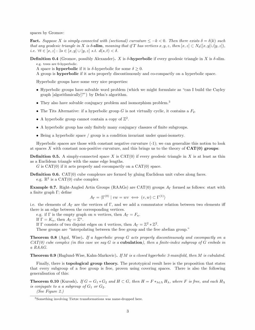
R
Rθ sinhR = θ
2eR
Figure 5: Hyperbolic circles have exponential circumference
and here we see the exponential divergence of geodesics and exponential growth which are twocharacteristics of negatively-curved spaces.
Note also the constant isopermetric inequality obtained from the above: frac2π(cosh(R)− 1)2π sinh(R)→1 as R→ 0 or as R→∞.
Moreover there are unique geodesics (unlike e.g. in spherical geometry) and the sum of the anglesin a triangle add up to < π: these are also characteristics of negatively-curved spaces.
Ideal triangles
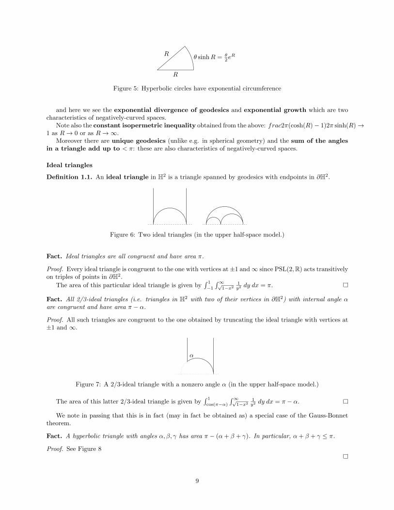
Definition 1.1. An ideal triangle in H2 is a triangle spanned by geodesics with endpoints in ∂H2.
Figure 6: Two ideal triangles (in the upper half-space model.)
Fact. Ideal triangles are all congruent and have area π.
Proof. Every ideal triangle is congruent to the one with vertices at ±1 and∞ since PSL(2,R) acts transitivelyon triples of points in ∂H2.
The area of this particular ideal triangle is given by∫ 1
−1
∫∞√1−x2
1y2 dy dx = π.
Fact. All 2/3-ideal triangles (i.e. triangles in H2 with two of their vertices in ∂H2) with internal angle αare congruent and have area π − α.
Proof. All such triangles are congruent to the one obtained by truncating the ideal triangle with vertices at±1 and ∞.
α
Figure 7: A 2/3-ideal triangle with a nonzero angle α (in the upper half-space model.)
The area of this latter 2/3-ideal triangle is given by∫ 1
cos(π−α)
∫∞√1−x2
1y2 dy dx = π − α.
We note in passing that this is in fact (may in fact be obtained as) a special case of the Gauss-Bonnettheorem.
Fact. A hyperbolic triangle with angles α, β, γ has area π − (α+ β + γ). In particular, α+ β + γ ≤ π.
Proof. See Figure 8
9

a c
b
a
bc
Figure 8: Here a, b, c stand for α, β, γ resp.; they represent the angles of the small white triangle, and alsothe areas of the shaded 2/3-ideal triangles by the previous Fact.
Fact. Triangles in H2 are cosh−1(2)-slim.
Proof. If T has sides S1, S2, S3, and z ∈ S1, d(z, S2 ∪ S3) ≤ cosh−1(2): if R = d(z, S2 ∪ S3), then half ofB(z,R) ⊂ T , so
Area(B(z,R)) < 2 Area(T )
2π cosh(R)− 2π < 2π
coshR < 2
Figure 9: That ball is at most half the triangle in area, and our desired inequality follows.
Hyperbolic sports!
Let’s think about baseball in hyperbolic space. How many outfielders would you need on a hyperbolicbaseball diamond? (Suppose the outfield is the area between 100 and 300 feet out from the pitcher.) Well,in Euclidean space E2, the outfield has area π
4 (3002 − 1002) ≈ 62, 832 square feet. In H2, the outfield wouldhave area 2π
4 (cosh 300 − cosh 100) 10100 square feet. Even assuming each outfielder could cover an areaof 104 square feet ... that doesn’t look good (due to exponential growth in this negatively-curved space.)
(You would also never see the ball coming: in E2 the visual size of a ball of radius R (e.g.) is 1πR . In H2,
it is 1π sinhR ∼
2πeR
.)Due to this exponential growth, real estate is cheap in hyperbolic space: one could imagine “a sketchy
real-estate agent in hyperbolic space” hawking spectacular (but relatively—or worse—worthless) timeshares.But back to sports—maybe we should choose another sport. Let’s try golf. Suppose you were taking a
shot at 300 feet, and you were 1 degree off. In E2, that would translate into your being ∼ 5.24 feet off at
300 feet. In H2, you would be 2π sinh(300)300 feet off. Oh well.
You would have the same problem/s with something like soccer: you would never see the ball coming,and the game would mostly involve passes to nowhere. Or, if one imagined a sort of rectangular field with
10

equally long goal lines on both sides, the center line would be extremely narrow, and then the game wouldmostly involve the goalies kicking the balls out of bounds.
Similarly, hyperbolic space would be a terrible place to go for a walk: you would never find your wayhome unless you were perfectly precise (due to the exponential divergence of geodesics.)
Some notes coming out of the tour ...
Definition 1.2. A (complete) n-manifold is hyperbolic if it is locally isometric to Hn.
Example 1.3. Σg is made from a regular hyperbolic 4g-gon with internal angles π2g and has area 2π(2g−2) =
2π|χ(Σg)|.
Figure 10: (Left) a torus formed by gluing the sides of a square; (right) a genus-2 surface formed by gluingthe sides of a regular hyperbolic octagon with angles π
4 .
Recall a proper geodesic metric space is hyperbolic if ∃δ > 0 s.t. all triangles are δ-slim (i.e. if T is ageodesic triangle in X with edges S1, S2, S3 and x ∈ S1, then d(x, S1 ∪ S2) ≤ δ.
A group is hyperbolic if it acts co-compactly and by isometries on a hyperbolic metric space.
Example 1.4. All finite groups are hyperbolic: in particular G finite =⇒ ΓG (a Cayley graph of G) isdiam(ΓG)-hyperbolic. Similarly, all compact hyperbolic metric spaces are δ-hyperbolic.
Fn is hyperbolic: it acts on a punctured (hyperbolic) surface.π1(Σg) (with g ≥ 2) is hyperbolic: it acts co-compactly and by isometries on Σg.Z2 is not ... why? (We will find out.)
1.2 The Fellow Traveller Property
Definition 1.5. If α : J → X is a (k, c)-quasi-isometric embedding, and J is an interval in R, then α iscalled a (k, c)-quasi-geodesic.
Note that geodesics need not be unique in hyperbolic metric spaces.
The universal cover of a hyperbolic surface Σg is H2. Since Σg is a simply-connected Riemannian manifoldlocally isometric to H2, so π1(Σg) acts properly and co-compactly on H2 if g ≥ 2.
If α : [a, b]→ X is a (k, c)-quasi-geodesic and X is δ-hyperbolic, then ∃D = D(k, c, δ) s.t. if [α(a), α(b)]is a geodesic (or even quasi-geodesic) going from α(a) to α(b), then
α([a, b]) ⊂ ND[α(a), α(b)] ⊂ N2D(α([a, b])).
The key fact used in the proof (which will be given below, along with a more precise statement of theProperty) is the exponential divergence of geodesics.
For now, we pause to state and prove an important corollary of the fellow traveller property:
Corollary. If f : X → Y is a quasi-isometric embedding, and Y is hyperbolic, then X is hyperbolic.
Proof. Suppose Y is δ-hyperbolic and f is a (k, c)-quasi-isometric embedding. Consider a (geodesic) trianglein X with sides s1, s2, s3.
Let s′i be a geodesic in Y with the same endpoints as f(si). By the fellow traveller property, there existsp′ ∈ s′i s.t. d(f(0), p′) ≤ D = D(k, c, δ). Since s′1, s
′2, s′3 form a geodesic triangle, ∃q′ ∈ s2 ∪ s3 (WLOG s3)
s.t. d(p′, q′) < δ and q′′ = f(q) ∈ f(s2) s.t. d(q′, q′′) < D.Then d(f(p), f(q)) < 2D + δ =⇒ d(n, q) < 1
k (2D + δ) + C =⇒ T is(
1k (2D + δ) + C
)-hyperbolic.
11

Figure 11: A quasi-isometry maps the (thin) black geodesic triangle on the right to the (thinnish) blackquasi-geodesic triangle on the right, which can be straightened to (is uniformly close to) the red geodesictriangle on the right.
Fact (Exponential divergence of geodesics). Suppose X is δ-hyperbolic, p lies on a geodesic [x, y] ∈ X, andα : [0, 1]→ X is a rectifiable path joining x to y. Then d(p, α(I)) ≤ δ log2(`(α)) + 1.
Figure 12: Any rectifiable curve (in particular, quasi-geodesic—grey) which is at least D away in Hausdorffdistance (red) from a geodesic (black) is exponentially (≥ 2(D−1)/δ) long.
Proof. “A picture I’m going to spend all sorts of time making precise.”
Parametrize α proportional to arc-length.Choose N ∈ N s.t. 2−(N+1)`(α) < 1 ≤ 2−N `(α), i.e. 2N ≤ `(α) < 2N+1, i.e. (since we have parametrized
∝ arc-length) 1 ≤ `(α[k
2N, k+1
2N
])< 2.
Consider the (geodesic) triangle [x, y], [α(0), α( 12 )], [α( 1
2 ), α(1)].Pick y1 ∈ [α(0), α( 1
2 )] ∪ [α( 12 ), α(1)] s.t. d(y1, p) < δ
If y1 ∈ [α(0), α( 12 )] (say), consider the triangle [α(0), α( 1
2 )], [α(0), α( 14 )], [α( 1
4 ), α( 12 )].
Choose y2 ∈ [α(0), α( 12 )]∪[α( 1
4 ), α( 12 )] s.t. d(y1, y2) < δ. Continue on until you find yN ∈
[α(k
2N
), α(k+12N
)]with d(yN , yN−1) < δ.
Figure 13: Starting with p on the geodesic (red dots), we find a sequence of points yi (successive red dots),each within δ of the previous, by δ-hyperbolicity. There are logarithmically many such points before we getwithin distance 1 of our rectifiable curve.
12
Then d(yN , p) < Nδ, and d(yN , α([0, 1]) < 1 since `(α[k
2N, k+1
2N
])< 2. (Consider the geodesic triangle with
endpoints α(
k2N
), α
(k+12N
), and yN .)
Hence we haved (p, α([0, 1])) ≤ Nδ + 1 ≤ δ log2(`(α)) + 1
We can use this to show, among other things, the following
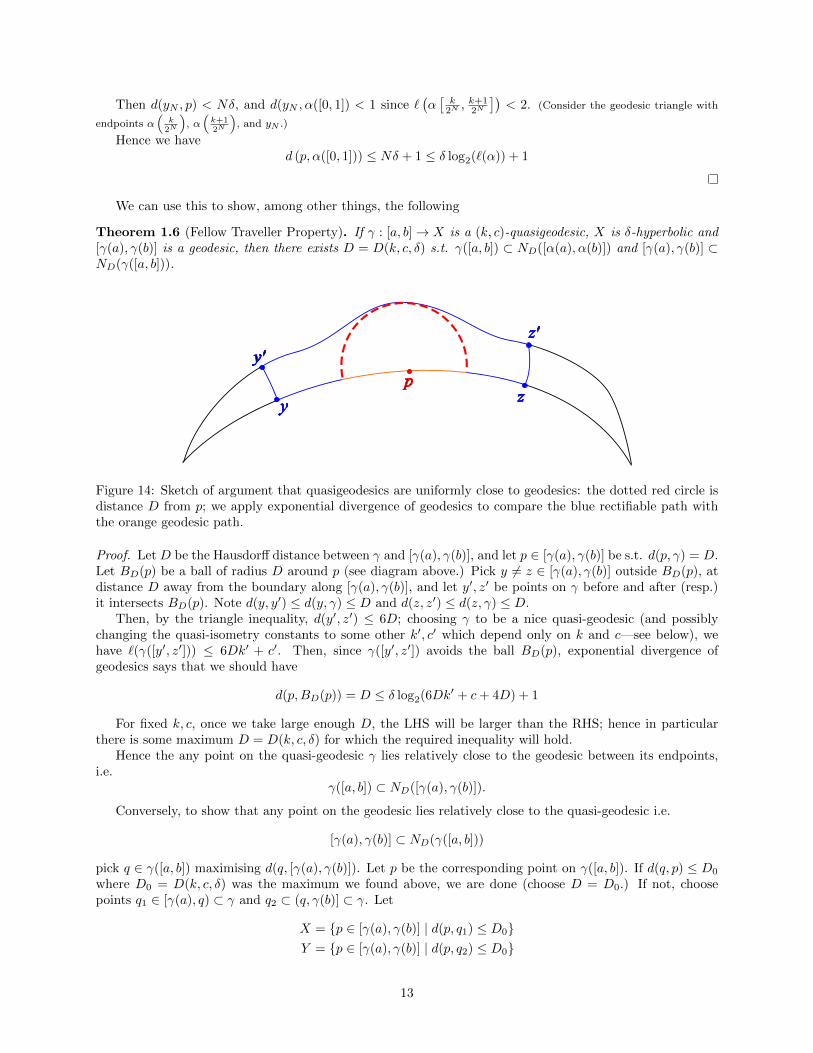
Theorem 1.6 (Fellow Traveller Property). If γ : [a, b]→ X is a (k, c)-quasigeodesic, X is δ-hyperbolic and[γ(a), γ(b)] is a geodesic, then there exists D = D(k, c, δ) s.t. γ([a, b]) ⊂ ND([α(a), α(b)]) and [γ(a), γ(b)] ⊂ND(γ([a, b])).
p
yz
y'
z'
Figure 14: Sketch of argument that quasigeodesics are uniformly close to geodesics: the dotted red circle isdistance D from p; we apply exponential divergence of geodesics to compare the blue rectifiable path withthe orange geodesic path.
Proof. Let D be the Hausdorff distance between γ and [γ(a), γ(b)], and let p ∈ [γ(a), γ(b)] be s.t. d(p, γ) = D.Let BD(p) be a ball of radius D around p (see diagram above.) Pick y 6= z ∈ [γ(a), γ(b)] outside BD(p), atdistance D away from the boundary along [γ(a), γ(b)], and let y′, z′ be points on γ before and after (resp.)it intersects BD(p). Note d(y, y′) ≤ d(y, γ) ≤ D and d(z, z′) ≤ d(z, γ) ≤ D.
Then, by the triangle inequality, d(y′, z′) ≤ 6D; choosing γ to be a nice quasi-geodesic (and possiblychanging the quasi-isometry constants to some other k′, c′ which depend only on k and c—see below), wehave `(γ([y′, z′])) ≤ 6Dk′ + c′. Then, since γ([y′, z′]) avoids the ball BD(p), exponential divergence ofgeodesics says that we should have
d(p,BD(p)) = D ≤ δ log2(6Dk′ + c+ 4D) + 1
For fixed k, c, once we take large enough D, the LHS will be larger than the RHS; hence in particularthere is some maximum D = D(k, c, δ) for which the required inequality will hold.
Hence the any point on the quasi-geodesic γ lies relatively close to the geodesic between its endpoints,i.e.
γ([a, b]) ⊂ ND([γ(a), γ(b)]).
Conversely, to show that any point on the geodesic lies relatively close to the quasi-geodesic i.e.
[γ(a), γ(b)] ⊂ ND(γ([a, b]))
pick q ∈ γ([a, b]) maximising d(q, [γ(a), γ(b)]). Let p be the corresponding point on γ([a, b]). If d(q, p) ≤ D0
where D0 = D(k, c, δ) was the maximum we found above, we are done (choose D = D0.) If not, choosepoints q1 ∈ [γ(a), q) ⊂ γ and q2 ⊂ (q, γ(b)] ⊂ γ. Let
X = p ∈ [γ(a), γ(b)] | d(p, q1) ≤ D0Y = p ∈ [γ(a), γ(b)] | d(p, q2) ≤ D0
13

and choose p1 ∈ X, p2 ∈ Y s.t. d(pi, qi) ≤ D0. If s and t are s.t. γ(s) = q1 and γ(t) = q2, then`(γ([s, t])) ≤ k′(2D0) + c′ and so
d(q, p) ≤ 1
2`(γ([s, t])) + maxd(p, q1), d(p, q2)
≤ k′D0 +c
2+D0
pp1 p2
q1q2
q
Figure 15: Sketch of argument that geodesics are uniformly close to quasigeodesics: each of the blue segmentshas length ≤ D0.
and if we now choose D = D1 = k′D0 + c2 +D0 then we have our desired result.
To show that we can take our quasi-geodesics to be nice (in particular, rectifiable), we will need thefollowing slightly technical lemma:
Lemma 1.7. Given a (k, c)-quasi-geodesic γ : [a, b]→ X in a geodesic metric space X, there exist k′ and c′
(depending on k and c) and a (k′, c′)-quasi-geodesic β : [a.b]→ X s.t.
(1) β(a) = γ(a) and β(b) = γ(b).
(2) The Hausdorff distance between γ([a, b]) and β([a, b]) is ≤ k + c.
(3) `(β[a, b]) ≤ k′d(β(a), β(b)) + c′.
Proof. Let S = ([a, b] ∩ Z) ∪ a, b = a = t0 ≤ t1 ≤ · · · ≤ tn = b.Choose β(t1) = γ(ti)∀ti ∈ S. Note that d(γ(ti), γ(ti+1) ≤ k(1)+c = k+c since γ is a (k, c)-quasi-geodesic.Choose β|[ti,ti+1] to have image a geodesic segment [β(ti, β(ti+1)] parametrized proportional to arc-length.
If p ∈ γ([ti, ti+1]), then d(p, γ(ti) ∪ γ(ti+1) ≤ k(
12
)+ c = k
2 + c.
If q ∈ β([ti, ti+1]), then d(q, γ(ti) ∪ γ(ti+1) ≤ k+c2 .
Thus the Hausdorff distance between β and γ is < k2 + c (since γ(ti)∪γ(ti+1) ⊂ β([a, b])∪γ([a, b]).) This
proves (2).Given t ∈ [a, b], let r(t) be a point in S closest to t. Then
d(β(s), β(t)) ≤ k + c
2+ d(β(r(s)), β(r(t)) +
k + c
2= d(γ(r(s)), γ(r(t)) + (k + c)
≤ k|r(s)− r(t)|+ c+ k + c
≤ k(|s− t|+ 1
2+
1
2
)+ (k + 2c) ∵ γ arc-length parametrization
= k|s− t|+ 2(k + c)
14
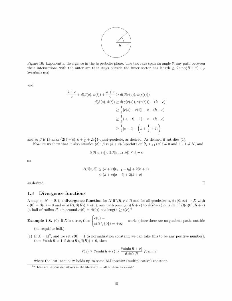
R r
Figure 16: Exponential divergence in the hyperbolic plane. The two rays span an angle θ; any path betweentheir intersections with the outer arc that stays outside the inner sector has length ≥ θ sinh(R + r) (by
hyperbolic trig)
and
k + c
2+ d(β(s), β(t)) +
k + c
2≥ d(β(r(s)), β(r(t)))
d(β(s), β(t)) ≥ d(γ(r(s)), γ(r(t)))− (k + c)
≥ 1
k|r(s)− r(t)| − c− (k + c)
≥ 1
k(|s− t| − 1)− c− (k + c)
≥ 1
k|s− t| −
(k +
1
k+ 2c
)and so β is
(k,max
2(k + c), k + 1
k + 2c)
-quasi-geodesic, as desired. As defined it satisfies (1).Now let us show that it also satisfies (3): β is (k + c)-Lipschitz on [ti, ti+1) if i 6= 0 and i+ 1 6= N , and
`(β([a, t1]), `(β([tn−1, b]) ≤ k + c
so
`(β[a, b]) ≤ (k + c)|tn−1 − t0|+ 2(k + c)
≤ (k + c)|a− b|+ 2(k + c)
as desired.
1.3 Divergence functions
A map e : N → R is a divergence function for X if ∀R, r ∈ N and for all geodesics α, β : [0,∞)→ X withα(0) = β(0) = 0 and d(α(R), β(R)) ≥ e(0), any path joining α(R+ r) to β(R+ r) outside of B(α(0), R+ r)(a ball of radius R+ r around α(0) = β(0)) has length ≥ e(r).6
Example 1.8. (0) If X is a tree, then
e(0) = 1
e(N \ 0) = +∞works (since there are no geodesic paths outside
the requisite ball.)
(1) If X = H2, and we set e(0) = 1 (a normalisation constant; we can take this to be any positive number),then θ sinhR > 1 if d(α(R), β(R)) > 0, then
`(γ) ≥ θ sinh(R+ r) >θ sinh(R+ r)
θ sinhR& sinh r
where the last inequality holds up to some bi-Lipschitz (multiplicative) constant.
6“There are various definitions in the literature ... all of them awkward.”
15

Figure 17: The geodesic triangle considered here consists of the red side, plus the two black sides. The dotted
geodesic is [α(R), β(R)].
Fact. A hyperbolic space X has an exponential divergence function.
Specifically, if X is δ-hyperbolic, then e(n) = max3δ, 2n−2δ is a divergence function.
It may also be shown that any non-hyperbolic space has a linear (or sublinear) divergence function
Proof. Suppose d(α(R), β(R)) > 3δ.Consider the geodesic triangle
α([0, R+ r]), β([0, R+ r]), [α(R+ r), β(R+ r)].
T is δ-slim, so there exists a point p ∈ [α(R+ r), β(R+ r)] s.t. d(p, α(R)) < δ. Suppose p ∈ β([0, R+ r]).Then R − δ < d(p, α(0)) < R + δ (two applications of the triangle inequality), and so p = β(t) where t ∈(R−δ,R+δ), and so d(p, β(R)) < δ, and so d(α(R), β(R)) < 2δ, which contradicts that d(α(R), β(R)) > 3δ.
So p ∈ [α(R + r), β(R + r)]. Then d(p, α(0)) ≤ R + δ, and, applying the triangle equality, we find thatBr−δ(p) ⊂ BR+r(α(0)) (otherwise we obtain some point q outside BR+r(α(0)) with d(α(0), q) ≤ d(α(0), p) +d(p, q) ≤ R+ δ + (r − δ) = R+ r—contradiction.)
Hence if γ is a path joining α(R+ r) to β(R+ r) outside BR+r(α(0)), we have d(p, γ) ≥ r − δ.Then, by exponential divergence of geodesics, r−δ ≤ d(p, γ) ≤ δ log2(`(γ))+1, and so `(γ) ≥ 2
r−δ−1δ .
There is also a converse which we will not prove here:
Theorem 1.9. If X is a proper geodesic metric space and has a superlinear divergence function e, i.e.
limn→∞
e(n)
n= +∞,
then X is hyperbolic.
1.4 Dehn presentations
A finite presentation Γ = 〈X;R〉 is a Dehn presentation if whenever w is a word in X and w ∼ id, thereexists a subword w0 of w which is “more than half a relator”, i.e. ∃ a word v0 s.t. `(v0) < `(w0) andv0w0 ∈ R.
Fact. If Γ has a Dehn presentation, the word problem is solvable in linear time.7
Proof. Consider the following algorithm:
• Given a word w in X, search w for subword which are more than half a relator
• If you don’t find any, w 6∼ id.
• If you find such a subword w0 (with v0w0 ∈ R and `(v0) < `(w0), then write w = aw0b ∼ av−10 b = w′
and note `(w′) < `(w).
• If w′ = id, stop (“and declare victory.”) If not, repeat above steps with w′ in the place of w.
Note that this will terminate in ≤ `(w) steps (e.g. by induction on `(w).)
7Linear in the length of the word, although this is also somewhat dependent on how substring search is implemented andhow operations are counted.
16
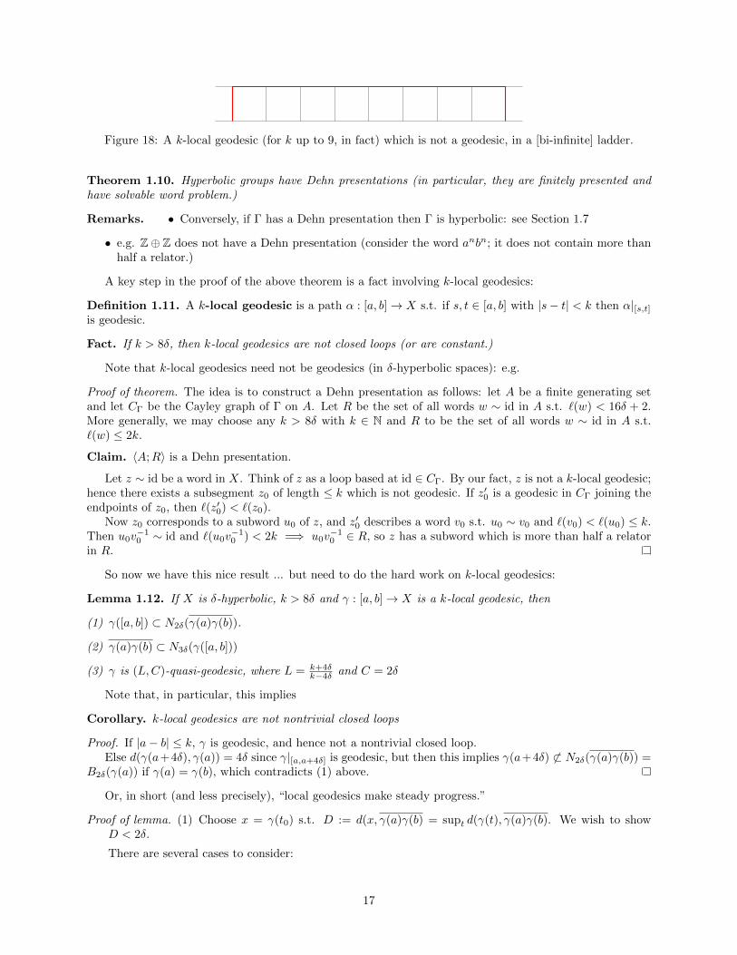
Figure 18: A k-local geodesic (for k up to 9, in fact) which is not a geodesic, in a [bi-infinite] ladder.
Theorem 1.10. Hyperbolic groups have Dehn presentations (in particular, they are finitely presented andhave solvable word problem.)
Remarks. • Conversely, if Γ has a Dehn presentation then Γ is hyperbolic: see Section 1.7
• e.g. Z⊕ Z does not have a Dehn presentation (consider the word anbn; it does not contain more thanhalf a relator.)
A key step in the proof of the above theorem is a fact involving k-local geodesics:
Definition 1.11. A k-local geodesic is a path α : [a, b]→ X s.t. if s, t ∈ [a, b] with |s− t| < k then α|[s,t]is geodesic.
Fact. If k > 8δ, then k-local geodesics are not closed loops (or are constant.)
Note that k-local geodesics need not be geodesics (in δ-hyperbolic spaces): e.g.
Proof of theorem. The idea is to construct a Dehn presentation as follows: let A be a finite generating setand let CΓ be the Cayley graph of Γ on A. Let R be the set of all words w ∼ id in A s.t. `(w) < 16δ + 2.More generally, we may choose any k > 8δ with k ∈ N and R to be the set of all words w ∼ id in A s.t.`(w) ≤ 2k.
Claim. 〈A;R〉 is a Dehn presentation.
Let z ∼ id be a word in X. Think of z as a loop based at id ∈ CΓ. By our fact, z is not a k-local geodesic;hence there exists a subsegment z0 of length ≤ k which is not geodesic. If z′0 is a geodesic in CΓ joining theendpoints of z0, then `(z′0) < `(z0).
Now z0 corresponds to a subword u0 of z, and z′0 describes a word v0 s.t. u0 ∼ v0 and `(v0) < `(u0) ≤ k.Then u0v
−10 ∼ id and `(u0v
−10 ) < 2k =⇒ u0v
−10 ∈ R, so z has a subword which is more than half a relator
in R.
So now we have this nice result ... but need to do the hard work on k-local geodesics:
Lemma 1.12. If X is δ-hyperbolic, k > 8δ and γ : [a, b]→ X is a k-local geodesic, then
(1) γ([a, b]) ⊂ N2δ(γ(a)γ(b)).
(2) γ(a)γ(b) ⊂ N3δ(γ([a, b]))
(3) γ is (L,C)-quasi-geodesic, where L = k+4δk−4δ and C = 2δ
Note that, in particular, this implies
Corollary. k-local geodesics are not nontrivial closed loops
Proof. If |a− b| ≤ k, γ is geodesic, and hence not a nontrivial closed loop.Else d(γ(a+4δ), γ(a)) = 4δ since γ|[a,a+4δ] is geodesic, but then this implies γ(a+4δ) 6⊂ N2δ(γ(a)γ(b)) =
B2δ(γ(a)) if γ(a) = γ(b), which contradicts (1) above.
Or, in short (and less precisely), “local geodesics make steady progress.”
Proof of lemma. (1) Choose x = γ(t0) s.t. D := d(x, γ(a)γ(b) = supt d(γ(t), γ(a)γ(b). We wish to showD < 2δ.
There are several cases to consider:
17
x
yz
y' z'
(a) (b)
44
<
<DD
x
yz
4
<
D - 3
y
y' z'
<
x
<
<D - 2
4
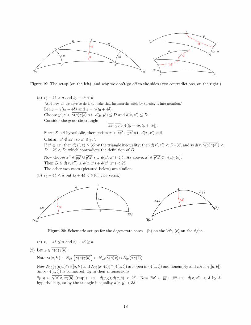
Figure 19: The setup (on the left), and why we don’t go off to the sides (two contradictions, on the right.)
(a) t0 − 4δ > a and t0 + 4δ < b
“And now all we have to do is to make that incomprehensible by turning it into notation.”
Let y = γ(t0 − 4δ) and z = γ(t0 + 4δ).
Choose y′, z′ ∈ γ(a)γ(b) s.t. d(y, y′) ≤ D and d(z, z′) ≤ D.
Consider the geodesic trianglezz′, yz′, γ([t0 − 4δ, t0 + 4δ]).
Since X s δ-hyperbolic, there exists x′ ∈ zz′ ∪ yz′ s.t. d(x, x′) < δ.
Claim. x′ /∈ zz′, so x′ ∈ yz′.If x′ ∈ zz′, then d(x′, z) > 3δ by the triangle inequality; then d(x′, z′) < D−3δ, and so d(x, γ(a)γ(b)) <D − 2δ < D, which contradicts the definition of D.
Now choose x′′ ∈ yy′ ∪ y′z′ s.t. d(x′, x′′) < δ. As above, x′ ∈ y′z′ ⊂ γ(a)γ(b).
Then D ≤ d(x, x′′) ≤ d(x, x′) + d(x′, x′′) < 2δ.
The other two cases (pictured below) are similar.
(b) t0 − 4δ ≤ a but t0 + 4δ < b (or vice versa.)
x
z
z'
(a)
(b)
4
<
D
<4
x
(a)
(b)
<<4
<4
Figure 20: Schematic setups for the degenerate cases—(b) on the left, (c) on the right.
(c) t0 − 4δ ≤ a and t0 + 4δ ≥ b.
(2) Let x ∈ γ(a)γ(b).
Note γ([a, b]) ⊂ N2δ
(γ(a)γ(b)
)⊂ N2δ(γ(a)x) ∪N2δ(xγ(b)).
Now N2δ(γ(a)x)∩γ([a, b]) and N2δ(xγ(b))∩γ([a, b]) are open in γ([a, b]) and nonempty and cover γ([a, b]).Since γ([a, b]) is connected, ∃y in their intersections.
∃p, q ∈ γ(a)x, xγ(b) (resp.) s.t. d(y, q), d(y, p) < 2δ. Now ∃x′ ∈ yp ∪ yq s.t. d(x, x′) < δ by δ-hyperbolicity, so by the triangle inequality d(x, y) < 3δ.
18

x
y
p q
(a) (b)
<2
<
Figure 21: Set-up for part (2).
(3) Roughly speaking, the idea is that“quasi-geodesics make [roughly] linear progress.”
Let k′ = k2 + 2δ > 6δ. Partition the interval [a, b] as a = t0 < t1 < · · · < tm ≤ b s.t. |ti − ti−1| = k′ and
η = |tn − b| < k′.
Notice that each γ|[ti−1,ti] is geodesic, since k′ < k. For each i, choose xi ∈ γ(a)γ(b) s.t. d(xi, γ(ti)) < 2δ.By the triangle inequality, d(xi, xi+1) > k′ − 4δ > 2δ > 0.
(a) (b)
<2
<2
x1
(t2)
x2
(t1)
>2
Figure 22: Crux of the argument: we choose projections which are sufficiently separated.
We wish to obtain something of the form d(γ(a), γ(b)) > m(k2 − 2δ) + (η− 2δ), and this we would obtain
if we can show that the xi proceed monotonically along γ(a)γ(b).
Claim. x0, x1, . . . , xm appear monotonically on γ(a)γ(b).
Fix i ∈ 0, 1, . . . ,m. Choose s0 = γ(ti+1 + 2δ) and s1 = γ(ti+1 − 2δ). We have corresponding geodesictriangles T0, T1.
γ(ti−1) γ(ti+1)
γ(ti)
xi−1 xi+1
xi
m′′
T0 T1< 2δ < 2δ
2δ 2δ
Figure 23: xi and m′′ are both within 2δ of γ(ti), and then xi−1 ∈ xim′′ puts xi−1 within 3δ of γ(ti)—contradiction.
Since T0 is δ-thin, every point of T0 lies within 3δ of γ(ti−1).; similarly, every point on T1 lies within 3δof γ(ti+1).
Since d(γ(ti), γ(ti+1) > 6δ, d(γ(ti), T1) > 3δ, and similarly d(γ(ti), T0) > 3δ.
Look at the [geodesic] quadrilateral with vertices s0, s1, xi−1, xi+1. Using the same argument as yesterdayinvolving δ-slim triangles and lower bounds on d(ti,−), ∃m′′ ∈ xi−1xi+1 s.t. d(m′′, γ(t)) < 2δ.
19

Suppose xi lies before xi−1 on γ(a)γ(b). Now d(xi−1, xi) > 2δ; consider the triangle with verticesxi,m
′′, γ(ti). Note xi−1 ∈ xim′′ and d(x, γ(ti)), d(γ(ti),m′′) < 2δ.
Since ∃x′i−1 ∈ xiγ(ti) ∪ γ(ti)m′′ with d(x′i−1, xi−1) < 2δ, we may conclude d(xi−1, γ(ti)) < 3δ, whichcontradicts the earlier statement that γ(ti) stays at least 3δ away from T0 and T1.
Now
d(γ(a), γ(b)) ≥ m(k′ − 4δ) + (η − 2δ)
≥(b− ak′− 1
)(k
2− 2δ) + η − 2δ
=k − 4δ
k + 4δ(b− a)− (
k
2− η)
≥ L(b− a)− 2δ
and after a similar bound in the other direction (d(γ(a), γ(b)) ≤ `(γ) ≤ mk′ + η) we are done.
1.5 Dehn functions
(Sometimes also known as isoperimetric functions.)
A Dehn function for a group Γ = 〈X;R〉 is a function f : N→ R s.t. if w ∼ id is a freely-reduced wordin X, then w can be written as a product of n ≤ f(`(w)) conjugates of relations, i.e. w =
∏ni=1 pir
εii p−1i ,
where ri ∈ R, pi ∈ Γ, and εi ∈ ±1.Consider the Cayley graph CΓ and add in a (2-)cell for each pir
εii p−1i to form a 2-dimensional CW complex
with π1(KΓ) = Γ.
Assign each edge length 1 and each cell area 1; then every closed loop α ⊂ KΓ bounds a [singular] diskDα of area ≤ f(`(α)).
e.g. KZ⊕Z = T 2 and KZ⊕Z = R2.
If M is a simply-connected Riemannian manifold of sectional curvature ≤ −ε < 0, then Area(D) < `(α)ε .
Example 1.13. (0) For Γ = Z = 〈a; 〉, or more generally Γ = Fm = 〈a1, . . . , am; 〉, f(n) = 0 is a Dehnfunction (since there are no relations.)
(1) For Γ = Z2 = 〈a, b | [a, b]〉, CΓ is “graph paper”, KΓ = R2.
w ∼ id =⇒ w a closed loop in the 1-skeleton of KΓ, so it bounds a disc Dw; by the (Euclidean)
isoperimetric inequality, the area of Dw is bounded above by π(`(w)2π
)2
= `(w)2
4π l hence fn = n2
4π is a
Dehn function.
To see that any Dehn function here must be at least quadratic, look at wk := akbka−kb−k ∼ id. Now`(wk) = 4k and the area of Dwk is k2; hence if g is any Dehn function for Z2 = 〈a, b | [a, b]〉, we must
have g(n) ≥ n2
16 .
(2) Γ = π1(Σ2) = 〈a, b, c, d | [a, b][c, d]〉 acts on H2 with fundamental domain a regular (all-45) octagon.
This gives a tessellation of H2 by such regular octagons; CΓ is the nerve of the tessellation (and is
quasi-isometric to H2.) KΓ = H2; KΓ has a tessellation by octagons dual to the first tessellation.
Let L be the length of each edge in CΓ and R be the area of an octagon in the dual tessellation.
w ∼ id gives rise to a loop α ∈ CΓ of length L · `(w); by the hyperbolic isometric inequality, Rn =Area(Dα) < `(α) = L · `(w)) if it takes n conjugates of relations to reduce w to id. So n < L
R`(w), and
so f(t) = LR t is a Dehn function for Γ.
“Now seems as good a time as any to introduce ... ”
20

1.6 Baumslag-Solitar groups and other counter-examples
Or, down the rabbit-hole of a family of standard counter-examples in combinatorial group theory.The Baumslag-Solitar group with parameters m and n is defined as BS(m,n) = 〈a, b | a−1bma = bn〉.Note that these are HNN extensions of Z2.
Some examples
• BS(1, 1) ∼= Z2
• BS(1, 2) = 〈a, b | a−1ba = b2〉 has exponential Dehn function
Relations look like
b
a
b b
a
A Cayley tree for the group (with the given presentation) consists of infinitely branched copies ofcross-sections which look like
Figure 24: One sheet of a Cayley graph for BS(1, 2). Note we have a−nban = b2n
.
Now consider w = b−1anb−1a−nbanba−n (go over one, go all the way down, go over one downstairs, go all the
way back up now in a different sheet, go back one over upstairs in the different sheet, come down again, then go back
one in the intersection of the two sheets and go all the way back up in the first sheet.)
an
b
an an
b
an
b
b
`(w) = 4n+ 4, but we may verify that the disk it spans has exponential area 2(2n− 1) (this is an obvious
upper bound; to make this argument fully rigorous we need to show this is the best possible disk for this word, i.e. that
it is a lower bound as well.)
• BS(2, 3) is not Hopfian, i.e. it is a proper quotient of itself
Other fun facts: the metabalian group G = 〈a, t | (t−1at)a(t−1at) = a2〉 has super-exponential Dehnfunction (i.e. its Dehn function grows faster than any finite tower of exponentials.)
21

1.7 Back to Dehn functions and hyperbolicity
We say that Γ = 〈X;R〉 has a linear isoperimetric inequality (LIP) if it has a Dehn function of the formf(n) = kn.
Observation. If Γ = 〈X;R〉 = 〈Y ;S〉, and 〈X;R〉 has a linear Dehn function, so does 〈Y ;S〉.
Proof. Suppose f(n) = kn is a Dehn function for 〈X;R〉.∃A s.t. for all y ∈ Y `X(y) ≤ kA.
∃B s.t. for all r ∈ R, r =∏Bj=1 pjs
εjj p−1j (after rewriting r as a word in Y .)
If w is a word in Y with w ∼ id, we can rewrite w in the alphabet X to obtain a freely-reduced z ∼ id
with `X(z) ≤ A`Y (w) and z =∏|S|i=1 qir
εii q−1i . Then
w =
|S|∏i=1
qi
B∏j=1
pijsεijij p−1ij
q−1i
and so |S| ≤ k`X(z) ≤ kA`Y (w); hence∑|S|i=1B ≤ kAB`Y (w), and so g(n) = kABn is a Dehn function for
〈Y ;S〉.
We may generalise the argument to obtain that: if f is a Dehn function for 〈X;R〉 ∼= 〈Y ;S〉, then ∃A,Bs.t. g9n) = Bf(An) is a Dehn function for 〈Y ;S.
Proposition 1.14. If Γ = 〈X;R〉 is a Dehn presentation, then Γ has a LIP.
Proof. If w is a word in X with w ∼ id, we get a sequence id = w0, w1, . . . , ws = w, where s ≤ `(w) andwj = ajujbj where ujvj ∈ R with `(uj) < `(vj).
uj
vj
bj
aj
Figure 25: One of linearly many relators obtained from a Dehn presentation.
Note that wj−1 = ajv−1j bj = aj−1ujbj−1, and that our sequence of wj ’s reduces w to id in s ≤ `(w)
steps.
Theorem 1.15. If Γ has a LIP, then Γ is hyperbolic.
Proof. The proof makes use of Van Kampen diagrams on putatively c-thick triangles in CΓ to obtain acontradiction. Hence all triangles in CΓ are δ-slim for some δ > 0, i.e. CΓ must be δ-hyperbolic.
Choose p ∈ xy s.t. d(p, yz ∪ xz) > c. WLOG (up to an additive fudge factor) p is a vertex of the Cayleygraph. Let λ ∈ (0, 1) (a concrete value for which can be backed out of the subsequent argument.)
Choose q to be the point in xp closest to p s.t. d(q, yz ∪ xz) = λc.Choose r to be the point in py closest to p s.t. d(r, yz ∪ xz) = λc.Choose q′, r′ ∈ xz ∪ yz s.t. d(q, q′) = d(r, r′) = λc.In the non-degenerate case, q′ ∈ xz and r′ ∈ yz. Choose s to be the closest point to q′ on q′z s.t.
d(s, yz) = λc and s′ ∈ yz s.t. d(s, s′) = λc.
22

q' r'
rq
s s'
Figure 26: A schematic illustration of the argument: filling a [hexagon inscribed inside a] thick triangle withquadratically many relators.
“By a small (≤ 2) fudge of these constants,” we can assume all these points are vertices.Write `1 := `(qr), `2 = `(q′s), and `3 = `(r′s′). WLOG `′ = `1 ≥ `2 + `3. By the triangle inequality,
`1 > 2(1− λ)c.Consider the hexagon H with vertices q, q′, s, s′, r′, r. `(H) = `1 + `2 + `3 + 3λc < 6`′. H bounds a
(singular) disk D.Let L0 = qr. Let ?(L0) be the union of all disks in H which touch L0. If K is the maximum length of
any relator in R, then the Area(?(L0)) (i.e. the number of 2-cells in ?(L0)) is ≥ `(L0)K = `′
K .
∃ a path L1 in ∂(?(L0)) joining qq′ to rr′ s.t. `(L1) ≥ `′ − 2K by the triangle inequality (as long asc10 K.) Then Area(?(L1)) ≥ `′−2K
K .Suppose f(n) = ρn is a Dehn function for Γ = 〈X;R〉; then Area(D) ≤ 6`′ρ.Since qq′, rr′ have length distance λc, we can iterate this process of taking the star ≥ λc
K times. Then
Area(D) ≥ Area(?(L0) ∪ · · · ∪ ?(Lλc
K))
≥ `′
K+`′ − 2K
K+ · · ·+ `′ − 2λC
K
≥ λc
K
(`′ − 2λC
K
)≥ λc
2K2`′
This gives a contradiction if we choose c > 2K2ρλ .
In the degenerate cases, [it is an exercise to check that] a simplified version of this argument similarlygives us the desired result.
In fact, we can prove:
Fact. If Γ has a Dehn function which is subquadratic, then Γ is hyperbolic.
Fact. If G and H are hyperbolic, then the free product G ∗H is hyperbolic.
Proof. G has a Dehn presentation 〈X;R〉 and H has a Dehn presentation 〈Y ;S〉.
23

q'
r'
rq
Figure 27: A degenerate case: a schematic illustration
Then 〈X ∪Y ;R∪S〉 is a Dehn presentation for G∗H: if w is freely reduced, then w = w1w2 · · ·wn wherewi ∈ G ⇐⇒ wi+1 ∈ H; then w ∼ id =⇒ ∃i : wi ∼ id =⇒ wi contains more than half a relator either inR or in S.
1.8 The conjugacy problem for hyperbolic groups
Theorem 1.16. The conjugacy problem is solvable for hyperbolic groups.
Let us first introduce a bit of notation, and a key lemma: given Γ = 〈X;R〉, a word w in X is fullyreduced (or cyclically reduced) if all cyclic conjugates of w (i.e. “take some stuff off front and stick it tothe back”) are freely reduced.
Lemma 1.17. If u and v are fully reduced and conjugate, then either
(1) `(u), `(v) ≤ 8δ + 1, or
(2) ∃ cyclic conjugates u′, v′ of u, v (resp.) and a word w of length ≤ 2δ + 1 s.t. wu′w−1 = v′.
Proof. Let w be a minimal-length word s.t. wu′w−1 = v′.
w w
u′
v′ p
q
u′1 u′2
v′1 v′2
Observation. If p is a vertex on Sv′ (the side associated to v′), then d (p, Su′) > `(w) − 12 , for if not then
∃q ∈ Su′ s.t. d(p, q) < `(w).
If now we write u′1 and u′2 to denote the parts of u′ up to and after q resp., and similarly write v′1 andv′2 to denote the parts of v′ before and after p resp. (see swag picture above), then w′(u′2u
′1)(w′)−1 = v′2v
′1,
and u′2u′1, v′2v
′1 are cyclic conjugates to u and v (resp.), and `(w′) < `(w), which contradicts that w was a
minimal-length conjugator between any pair of cyclic conjugates for u′ and v′.Now suppose p is a midpoint of Sv′ and that `(w) > 2δ + 1, so ∃q on a vertical side of the rectangle s.t.
d(p, q) < 2δ.
p
q
< 2δy
x
`(v)2
24

Then d(q, y) > `(v)2 − 2δ and d(q, x) = `(w)− d(q, y) < `(w)− `(v)
2 + 2δ, so
`(w)− 1
2≤ d(p, x) ≤ d(x, q) + 2δ ≤ `(w) + 4δ − `(v)
2
and hence `(v)2 ≤ 4δ + 1
2 , i.e. `(v) ≤ 8δ + 1.Symmetrically, `(u) ≤ 8δ + 1.So either `(w) ≤ 2δ + 1, or `(v), `(u) ≤ 8δ + 1, as desired.
Solution to conjugacy problem. (0) Let B1 = w | `(w) ≤ 2δ + 1. B1 is finite.
If u, v are short (`(u), `(v) ≤ 8δ+1 and are conjugate, then let wuv be s.t. wuvuw−1uv = v. Let B2 = wuv.
Since there are finitely many pairs of such short words, B2 is finite.
Let B = B1 ∪ B2.
(1) If u and v are words in X, first conjugate and reduce until you find u′, v′ conjugate to u, v (resp.) fullyreduced. Note `(u′) ≤ `(u) and `(v′) ≤ `(v).
(2) Check if wu′′w−1 = v′′ ∀w ∈ B where u′′ and v′′ range over all cyclic conjugates of u′ and v′ (resp.)
1.9 Finiteness in hyperbolic groups
We remark also that stronger results holds:
Theorem 1.18. Γ hyperbolic =⇒ there are only finitely many conjugacy classes of finite subgroups of Γ.
Remark. We note that this result can be generalised as follows: if Γ acts properly and co-compactly on asimply-connected negatively (non-positively) curved manifold, the same conclusion holds.
Proof. The idea is this: pick x0 ∈ X. If H ⊂ Γ is finite, consider H(x0). Then H(x0) has a well-definedbarycenter (center of mass), because the distance function is convex. Since H(x0) is preserved by H, sois its barycenter; hence H has a fixed point h0 ∈ X. Now ∃ compact K ⊂ X which contains a pointΓ-equivalent to any point in X (i.e. which contains a fundamental domain.) Hence (implicitly assuming
X = Cay(Γ)) ∃γ0 s.t. γ0(h0) ∈ K =⇒ γ0Hγ−10 ⊂ γ ∈ Γ | γ(K) ∩ K 6= ∅, which is finite (since
γ0Hγ−10 (γ0h0) = γ0Hh0 = γ0h0 ∈ (γ0Hγ
−10 )K ∩K.
To make this rigorous we will use the following
Lemma 1.19. If X is δ-hyperbolic and Y ⊂ X is non-empty and bounded, let rY = infρ > 0 | ∃x ∈X s.t. Y ⊂ B(x, ρ) be the radius of Y . Then for all ε > 0, the set Cε(Y ) := x ∈ X | Y ⊂ B(x, rY + ε)(the set of “ε-candidates for barycenters”) has diameter ≤ 4δ + 2ε.
Proof. Pick x1, x2 ∈ Cε(Y ), let m be the midpoint of x1x2, and pick y ∈ Y s.t. d(y,m) ≥ rY .
ym
x2
x1
< r + ε
≥ r
25

Then ∃p ∈ xiy s.t. d(p,m) < δ. WLOG we let xi = x1.
Now d(p, x1) ≥ d(x,m)− δ = d(x1,x2)2 − δ, and so
d(p, y) = d(x1, y)− d(x1, p)
≤ d(x1, y) + δ − d(x1, x2)
2
< rY + ε+ δ − d(x1, x2)
2
d(m, y) ≤ d(p, y) + δ ≤ rY + ε+ 2δ − d(x1, x2)
2
but d(m, y) ≥ rY , and so rY ≤ rY + ε+ 2δ − d(x1,x2)2 , or d(x1, x2) ≤ 2(2δ + ε) = 4δ + 2ε.
Hence the Cε(Y ) (the ε-coarse barycenters of Y ) are coarsely well-defined.Suppose H ⊂ Γ is finite; identify H with the set of vertices H(id) ⊂ CΓ. Let C1(H) be the set of 1-coarse
barycenters.Since diam(C1(H)) ≥ 1, ∃ vertex γ ∈ C1(H).Since H leaves H invariant, H(C1(H)) = C1(H), so γ−1Hγ(γ−1(C1(H))) = γ−1(C1(H)). But id ∈
γ−1(C1(H)) since γ ∈ C1(H), so γ−1(C1(H)) ⊂ B4δ+2(id) =: R.Hence ∀β ∈ γ−1Hγ, β(R) ∩ R 6= ∅, i.e. γ−1Hγ ⊂ α ∈ Γ | α(R) ∩ R 6= ∅, which is finite. Since every
finite subgroup is conjugate into R, and R is finite, we conclude that there are only finitely many possibilitiesfor the conjugacy class of H.
Corollary. If A ⊂ Γ is abelian, then A is virtually cyclic.
Proof. If A contains an infinite-order element α, then A ⊂ Z(α), and hence is virtually infinite cyclic (seefollowing section.)
If A is abelian, not virtually cyclic, and does not contain an infinite-order element, then it containsinfinitely many isomorphism classes of finite subgroups, which is impossible since conjugate subgroups areisomorphic.
Fact. Γ hyperbolic =⇒ Γ contains only finitely many conjugacy classes of finite-order elements.In particular, there exists an upper bound on the order of a finite-order element.
Proof. Morally, the result holds because in a hyperbolic space the distance function is convex, and so we have uniquely-defined
barycenters.
Let 〈X;R〉 be a Dehn presentation for Γ.Suppose γ ∈ Γ s.t. γn = id, n > 1, and γ has minimal length of any element in its conjugacy class.Let w be a minimal-length word in X s.t. w ∼ γ. Then wn ∼ id and hence wn contains more than half
a relator in R, i.e. ∃r = r1r2 ∈ R of wn with `(r1) > `(r2) and r1 is a subword of wn.If r1 is contained in a copy of w, then w = ar1b ∼ ar−1
2 b ∼ γ, and hence w was not a minimal-lengthrepresentation of γ: contradiction.
Otherwise, if `(w) > `(r1), then w = utv where vu = r1, since r1 is a subword of ww but not of w. Nowtake a conjugate u−1wu = tvu = tr1 ∼ tr−1
2 ; `(tr1) > `(tr−12 ), which contradicts that γ was a minimal-length
representative of its conjugacy class.Hence `(w) ≤ R := max`(r) | r ∈ R, and so every finite-order element of Γ is conjugate to a word of
length ≤ R. There are only finitely many such words, and we are done.
One moral of this story is that “there’s a lot of juice in the Dehn presentation.”
Remark. There exists a finitely-presented group which contains an isomorphic copy of every other finitely-presented group (see e.g. de la Harpe for references.)
26

1.10 Cyclic subgroups in hyperbolic groups
Theorem 1.20. If Γ is hyperbolic and γ ∈ Γ has infinite order, then the map Z → Γ given by n 7→ γn
is a quasi-isometric embedding, i.e. ∃k, c s.t. nk − c ≤ dΓ(1, γn) ≤ kn + c (note that n = dZ(1, n) and
dΓ(1, γn) = `(γn).)We also describe this by saying that “cyclic subgroups [of hyperbolic groups] are undistorted.”
Remarks. (1) `(γn) ≤ `(γ), since we can take a word w = γ; then `(w) = `(γ) and `(wn) = n`(w) = n`(γ).
(2) This property is not exclusive to hyperbolic groups.
e.g. in Z⊕ Z = 〈a, b | [a, b]〉, `((arbs)n) = n(r + s) = n(`(arbs)).
(3) 〈a〉 is distorted in BS(1, 2) = 〈a, b | bab−1 = a2〉: we may show (inductively on n) that a2n = bnab−n
(e.g. b2ab−1 = b(bab−1)b−1 = ba2b−1 = (bab−1)2 = (a2)2 = a4) and so `(a2n) ≤ 2n+1. This is k2n−cfor any fixed choice of k and c as long as n is large enough.
Moreover, BS(1, 2) is not isomorphic to a subgroup of a hyperbolic group.
In fact, BS(m,n) is never a subgroup of a hyperbolic group (e.g. BS(1, 1) ∼= Z⊕ Z.)
(4) On the other hand, there do exist finitely-presented subgroups of hyperbolic groups which are nothyperbolic.
Gromov asked the question: does there exist a finitely-presented group Γ s.t. Γ is not hyperbolicand does not contain any BS(m,n) as a subgroup? (Or, put differently, are there other obstructions tohyperbolicity than the Baumslag-Solitar groups?)
This was answered in the affirmative by Brady in 1999—in fact there exist torsion-free finitely-presentedcounter-examples; however his examples have no finite K(Γ, 1).
Definition 1.21. A finite K(Γ, 1) is a finite cell complex X s.t. π1(X) ∼= Γ and X is contractible (i.e.πn(X) = 1 for all n, which is equivalent to πn(X) = 1 for all n > 1 by Whitehead’s theorem.)
It is known that all torsionfree hyperbolic groups have finite K(Γ, 1).We may also speak of virtually finite K(Γ, 1).
New question: What if we assume finite K(Γ, 1)?
Corollary. If Γ is hyperbolic, and γ ∈ Γ has infinite order, then Z(γ)/〈γ〉 is finite, where Z(γ) denotes thecentralizer β ∈ Γ | βγβ−1 = γ
Proof. Suppose Z→ Γ given by n 7→ γn is a (k, c)-quasi-isometric embedding.Pick a geodesic word w s.t. w = γ; then wn = γn is a (k, c)-quasigeodesic path in CΓ.By the fellow traveller property, ∃L = L(k, c) s.t. 1γn ⊂ NL(Pwn) where Pwn is the path determined by
wn.Suppose β ∈ Z(γ). Choose n > 0 s.t. d(1, γn) > 2`(β) + 4δ + 4.
id
βc
βγn = γnβ
γa
1γn
β(1γn)
2δ
Supposing d(1, γn) `(γ), we may choose a vertex a which is almost a midpoint, i.e. a ∈ 1γn and
d(a, id), d(a, γn) ≥ d(1,γn)2 − 1
2 .Then d(a, id), d(a, γn) > 2δ implies that there exists a vertex c ∈ β(1γn) s.t. d(a, c) ≤ 2δ + 1
2 .Now every point on the path determined by wn lies within `(w) of the form γj for some 0 ≤ j ≤ n, so,
by the fellow traveller property (as applied above) ∃j ∈ N s.t. d(a, γj) ≤ L + `(w); similarly ∃k ∈ N s.t.d(c, βγk) ≤ L+ `(w).
Hence d(γj , βγk) ≤ 2(δ+L+ `(w)) + 12 and so `(βγk−j) ≤ 2(δ+L+ `(w)) + 1
2 =: C. Thus every coset inZ(γ)/〈γ〉 has a representative of length ≤ C. Since there are only finitely many words of length ≤ C, thereare only finitely many cosets.
27

We may compare the above corollary to Preissman’s Theorem, which states that if M is a negatively-curved closed manifold, then the only abelian subgroups of π1(M) are (isomorphic to) Z or the trivialsubgroup.
From this corollary we may deduce
Corollary. No hyperbolic group contains an isomorphic copy of Z⊕ Z.Hence no BS(n, n) is contained in a hyperbolic Γ.
Another corollary of Theorem 1.20 is the following:
Corollary. If Γ is hyperbolic, γ ∈ Γ has infinite order, and hγth−1 = γs for some h ∈ Γ then s = ±t.
Proof. If γs = hγth−1 for some h ∈ Γ and s > t, then inductively γsn
= hnγtn
h−n e.g.
h2γt2
h−2 = h(hγt2
h−1)h−1
= h(hγth−1) · · · (hγth−1)h−1
= hγs · · · γsh−1
= hγsth−1
= (hγth−1) · · · (hγth−1)
= γs · · · γs = γs2
Suppose n 7→ γn is a (k, c)-quasi-isometric embedding. Then
sn
k− c ≤ `(γs
n
) = `(hnγtn
h−n) ≤ 2n`(h) + tn`(γ)
for all n, but this is impossible if s > t.
Combining the above two corollaries, we may conclude
Corollary. H ⊂ Γ hyperbolic =⇒ H 6∼= BS(m,n) for m 6= ±n.
Corollary. No hyperbolic group contains an isomorphic copy of Z⊕ Z (so no BS(n, n) are contained in Γeither.)
And now, after exploring these consequences, we turn to the proof of the theorem itself:
Proof of Theorem 1.20. It suffices to prove that ∃R ∈ Z>0 s.t. d(1, gnR) > n for all n, since this would implyd(1, gk) ≥ b kRc − (R − 1)`(g), where `(g) is bounded by d(1, g), but on the other hand d(1, gk) ≤ `(g)k, sowe would have
k
R− (R− 1)`(g)− 1 ≤ d(1, gk) ≤ `(g)k.
By equivariance,|s− t|R
< (R− 1)`(g) + 1 ≤ d(γs, γt) ≤ `(g)|s− t|
so n 7→ γn would be a (k, c)-quasi-isometric embedding (with k = max`(g), 1R and c = (R− 1)`(g) + 1.)
To proceed with this we will need the following
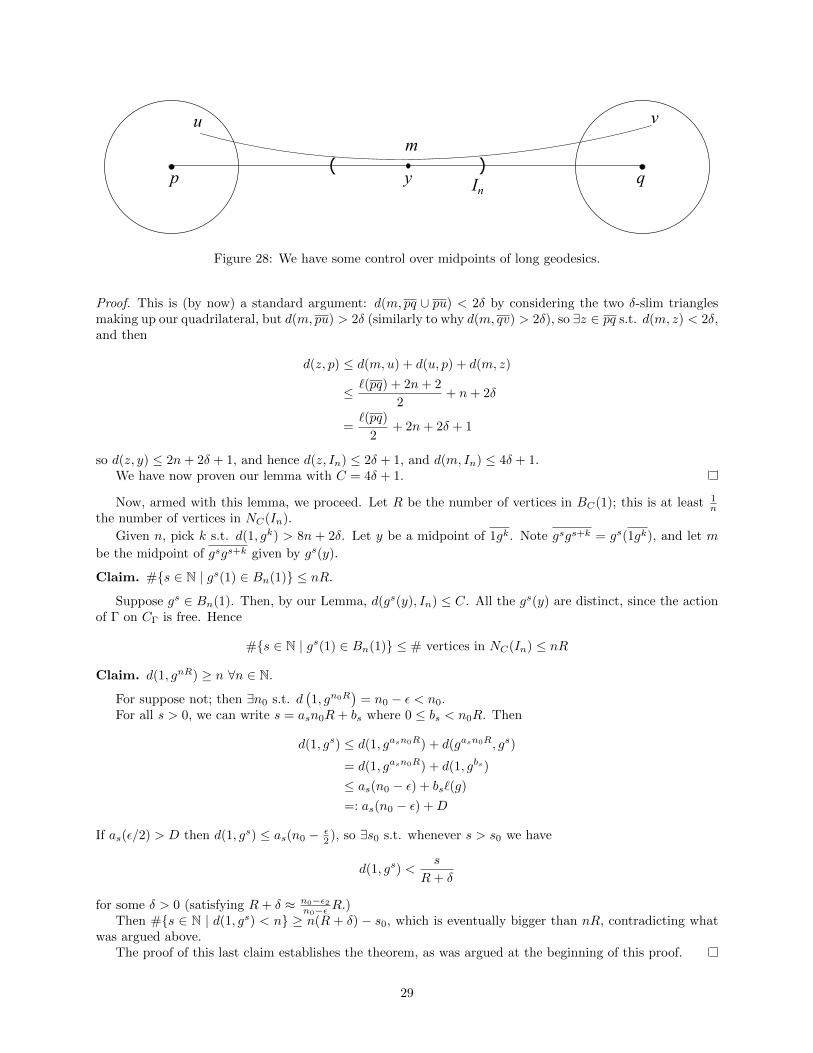
Lemma 1.22. Given δ > 0, ∃C > 0 s.t. if n ∈ N, CΓ is δ-hyperbolic, p and q are vertices in CΓ with`(pq) > 8n+2δ, In is a subinterval of pq of radius n about y, u ∈ Bn(p) and v ∈ Bn(q), and m is a midpointof uv, then d(m, In) ≤ C.
“It’s always a mistake to state the lemma before drawing the picture.”
28
yp q
u v
m( )
In
Figure 28: We have some control over midpoints of long geodesics.
Proof. This is (by now) a standard argument: d(m, pq ∪ pu) < 2δ by considering the two δ-slim trianglesmaking up our quadrilateral, but d(m, pu) > 2δ (similarly to why d(m, qv) > 2δ), so ∃z ∈ pq s.t. d(m, z) < 2δ,and then
d(z, p) ≤ d(m,u) + d(u, p) + d(m, z)
≤ `(pq) + 2n+ 2
2+ n+ 2δ
=`(pq)
2+ 2n+ 2δ + 1
so d(z, y) ≤ 2n+ 2δ + 1, and hence d(z, In) ≤ 2δ + 1, and d(m, In) ≤ 4δ + 1.We have now proven our lemma with C = 4δ + 1.
Now, armed with this lemma, we proceed. Let R be the number of vertices in BC(1); this is at least 1n
the number of vertices in NC(In).
Given n, pick k s.t. d(1, gk) > 8n + 2δ. Let y be a midpoint of 1gk. Note gsgs+k = gs(1gk), and let m
be the midpoint of gsgs+k given by gs(y).
Claim. #s ∈ N | gs(1) ∈ Bn(1) ≤ nR.
Suppose gs ∈ Bn(1). Then, by our Lemma, d(gs(y), In) ≤ C. All the gs(y) are distinct, since the actionof Γ on CΓ is free. Hence
#s ∈ N | gs(1) ∈ Bn(1) ≤ # vertices in NC(In) ≤ nR
Claim. d(1, gnR) ≥ n ∀n ∈ N.
For suppose not; then ∃n0 s.t. d(1, gn0R
)= n0 − ε < n0.
For all s > 0, we can write s = asn0R+ bs where 0 ≤ bs < n0R. Then
d(1, gs) ≤ d(1, gasn0R) + d(gasn0R, gs)
= d(1, gasn0R) + d(1, gbs)
≤ as(n0 − ε) + bs`(g)
=: as(n0 − ε) +D
If as(ε/2) > D then d(1, gs) ≤ as(n0 − ε2 ), so ∃s0 s.t. whenever s > s0 we have
d(1, gs) <s
R+ δ
for some δ > 0 (satisfying R+ δ ≈ n0−ε2n0−ε R.)
Then #s ∈ N | d(1, gs) < n ≥ n(R + δ) − s0, which is eventually bigger than nR, contradicting whatwas argued above.
The proof of this last claim establishes the theorem, as was argued at the beginning of this proof.
29

1.11 Quasiconvexity
Definition 1.23. If X is a proper geodesic metric space, we say A ⊂ X is k-quasiconvex if for all a1, a2 ∈ A,a1a2 ∈ Nk(A) (for all geodesics a1a2.
k
Figure 29: An example of a k-quasiconvex set in the plane
If Γ is a group with presentation Γ = 〈X;R〉, and H ⊂ Γ is a subgroup, then H is quasiconvex (i.e.k-quasiconvex for some k ≥ 0) if H is a quasiconvex subset of CΓ.
Example 1.24. • Cyclic groups are quasiconvex subsets of hyperbolic groups.
• Finite-index subgroups are quasiconvex (since they are coarsely dense.)
• Note that quasiconvexity is dependent on the presentation.
e.g. in Z⊕ Z = 〈a, b | [a, b]〉, 〈a〉 is quasiconvex but 〈ab〉 is not
Figure 30: Paths of the form anbn are geodesics in Z ⊕ Z = 〈a, b|[a, b]〉, but can get arbitrarily far from〈ab〉 ⊂ 〈a, b|[a, b]〉.
However in 〈b, ab | [b, ab]〉 ∼= Z⊕ Z, 〈ab〉 is quasiconvex but 〈a〉 is not.
Exercise. In the hyperbolic setting, quasiconvexity of a subgroup is independent of the choice of generatingset.
Hint: fellow traveller property.
Theorem 1.25. If Γ is hyperbolic and H ⊂ Γ is quasiconvex, then H is hyperbolic. In particular, H isfinitely presented.
Remarks. (1) (Brady) There exists a hyperbolic group with non-hyperbolic subgroups (i.e. the aboveresult is not trivial.)
(2) There is a general construction, due to Rips, which, given a finitely-generated group G, builds a short
exact sequence 1 N Γ G 1 where Γ is hyperbolic.
If G is infinite, then N is finitely generated but not finitely presented.
(3) The converse does not hold: hyperbolic subgroups of hyperbolic groups need not be quasiconvex.
The counterexamples here are rather canonical—they come from hyperbolic 3-manifolds.
e.g. take a surface Σ of genus g ≥ 2 and define S = Σ × [0, 1], let φ : S → S be a psuedo-Anosov(“generic”) self-homeomorphism. Then the mapping torus Mφ = H3/Γ, but π1(Γ) ⊂ Γ is not quasicon-vex.
30
To prove this we will first need a
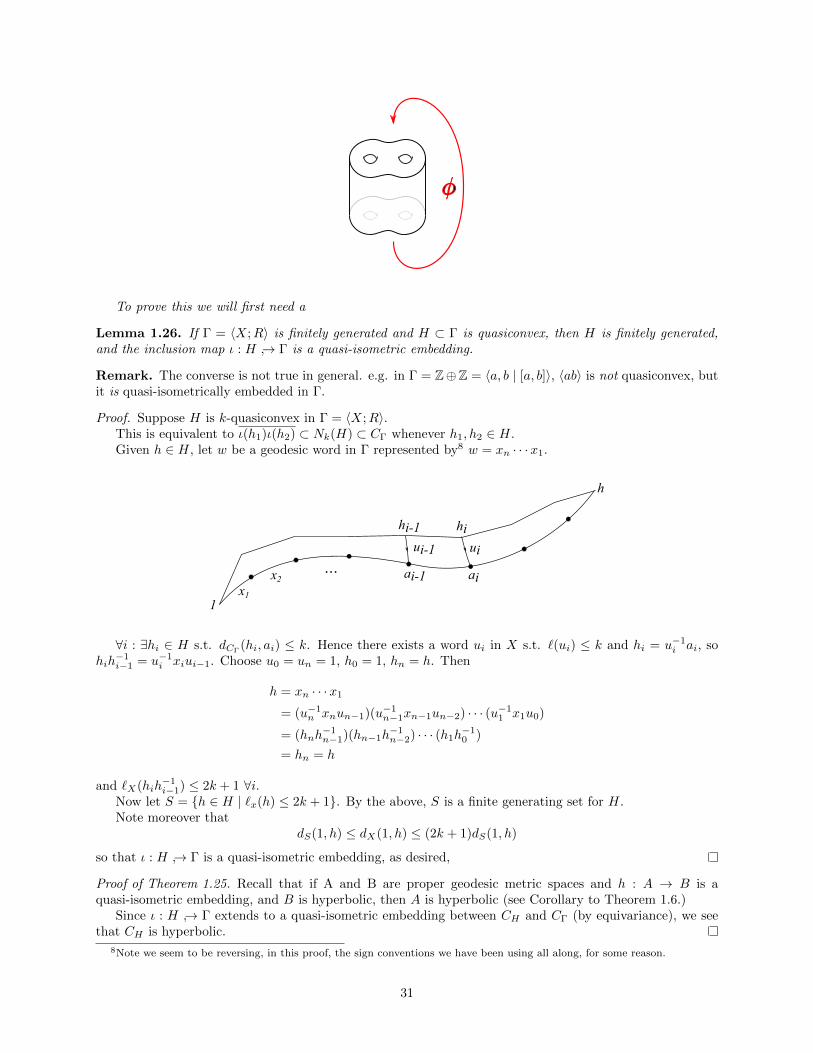
Lemma 1.26. If Γ = 〈X;R〉 is finitely generated and H ⊂ Γ is quasiconvex, then H is finitely generated,and the inclusion map ι : H → Γ is a quasi-isometric embedding.
Remark. The converse is not true in general. e.g. in Γ = Z⊕Z = 〈a, b | [a, b]〉, 〈ab〉 is not quasiconvex, butit is quasi-isometrically embedded in Γ.
Proof. Suppose H is k-quasiconvex in Γ = 〈X;R〉.This is equivalent to ι(h1)ι(h2) ⊂ Nk(H) ⊂ CΓ whenever h1, h2 ∈ H.Given h ∈ H, let w be a geodesic word in Γ represented by8 w = xn · · ·x1.
ai-1 ai
hi-1 hiui-1 ui
1
h
x1x2
...
∀i : ∃hi ∈ H s.t. dCΓ(hi, ai) ≤ k. Hence there exists a word ui in X s.t. `(ui) ≤ k and hi = u−1i ai, so
hih−1i−1 = u−1
i xiui−1. Choose u0 = un = 1, h0 = 1, hn = h. Then
h = xn · · ·x1
= (u−1n xnun−1)(u−1
n−1xn−1un−2) · · · (u−11 x1u0)
= (hnh−1n−1)(hn−1h
−1n−2) · · · (h1h
−10 )
= hn = h
and `X(hih−1i−1) ≤ 2k + 1 ∀i.
Now let S = h ∈ H | `x(h) ≤ 2k + 1. By the above, S is a finite generating set for H.Note moreover that
dS(1, h) ≤ dX(1, h) ≤ (2k + 1)dS(1, h)
so that ι : H → Γ is a quasi-isometric embedding, as desired,
Proof of Theorem 1.25. Recall that if A and B are proper geodesic metric spaces and h : A → B is aquasi-isometric embedding, and B is hyperbolic, then A is hyperbolic (see Corollary to Theorem 1.6.)
Since ι : H → Γ extends to a quasi-isometric embedding between CH and CΓ (by equivariance), we seethat CH is hyperbolic.
8Note we seem to be reversing, in this proof, the sign conventions we have been using all along, for some reason.
31
Corollary. If Γ is hyperbolic, then H ⊂ Γ quasiconvex ⇐⇒ H → Γ is a quasi-isometric embedding.In particular, for hyperbolic groups quasiconvexity of subgroups is independent of the choice of generators.
Proof. The Lemma gives us the =⇒ direction.For the other direction, suppose Γ is δ-hyperbolic, and H → Γ is a (k, c)-quasi-isometric embedding. If
h1h2 is a geodesic in CH , ι(h1h2) is a (k, c)-quasi-geodesic in CΓ.The fellow traveller property now tells us that ∃L = L(k, c, δ) s.t. NL(ι(h1h2)) ⊃ ι(h1)ι(h2) where
ι(h1)ι(h2) is a geodesic in CΓ joining h1 to h2.Thus every point in ι(h1h2) lies within k + c of an element of H =⇒ ι(h1)ι(h2) lies within k + c+ L of
H =⇒ H is (k + c+ L)-quasiconvex.
Quasiconvexity can also be used to formulate a common generalization (for hyperbolic groups) of thefollowing classical theorem/s
Theorem 1.27 (Howson’s Theorem). If H1, H2 ⊂ Fn are finitely-generated, then H1 ∩ H2 is finitely-generated.
To state the other result we first require some terminology:
Definition 1.28. H ⊂ Isom(Hn) is9 convex co-compact if ∃x0 ∈ Hn (or ∀x0 ∈ HHn: these formulationsare equivalent by equivariance [?]) s.t. the orbit map τ : Γ → Hn given by γ 7→ γ(x0) is a quasi-isometricembedding10.
To see why the name “convex co-compact”: let Λ(Γ) := Γx0 ∩ ∂Hn. (In fact, Γ also has a boundary ∂Γand τ extends to a map τ : Γ ∪ ∂Γ→ Hn ∪ ∂Hn.)
Now the convex hull CH(Λ(Γ)), i.e. the smallest closed Γ-invariant convex subset of Hn containing Λ(Γ)in its closure, is formed by the union of all ideal simplices with endpoints in Λ(Γ).
Hence k-quasiconvexity =⇒ CH(Λ(Γ)) ⊂ NL(Γx0) =⇒ CH(Λ(Γ))/Γ is compact, and convex as asubset of Hn/Γ.
Theorem 1.29 (Susskind). If Γ ⊂ Isom(Hn) is discrete, and H1, H2 ⊂ Γ are convex co-compact, thenH1 ∩H2 is convex co-compact.
The common generalisation is this:
Theorem 1.30. If Γ is hyperbolic and H1, H2 ⊂ Γ are quasiconvex, then H1 ∩H2 is quasiconvex.
Note that
Theorem 1.31 (Thurston). Γ convex co-compact but not co-compact and H ⊂ Γ finitely generated =⇒ Hconvex co-compact
Definition 1.32. Γ has the finitely-generated intersection property (FGIP) if H1, H2 ⊂ Γ finitely-generated =⇒ H1 ∩H2 finitely-generated.
From these results of Thurston and of Susskind we may conclude
Corollary. If Γ ⊂ Isom(Hn) is convex co-compact but not compact, then Γ has the FGIP.
Example 1.33. Let Σ be a surface of genus g ≥ 2 and φ : Σ→ Σ be a psuedo-Anosov self-homeomorphism.Let M = Mφ be the mapping torus of φ. Note φ pseudo-Anosov implies Mφ = H3/Γ (for some hyperbolicgroup Γ), by geometrization.
There exists a short exact sequence 1 π1(Σ) Γ Z 1 and we may write Γ =
〈π1(Σ), t | tat−1 = φ(a) ∀a ∈ π1(Σ)〉, “the standard form for a HNN extension”.Notice that the limit sets agree: Λ(π1(Σ)) = Λ(Γ), since π1(Σ) C Γ and Λ(Γ) is the smallest closed
non-empty Γ-invariant subset.
9Fun facts: Isom(H2) ∼= PSL(2,R); Isom(H3) ∼= PSL(2,C).10By the Lemma above, this is equivalent to quasiconvexity of Γ.
32

Now CH(Λ(π1(Σ))) = CH(Λ(Γ)), so CH(Λ(π1(Σ)))/π1(Σ) is not compact, i.e. π1(Σ) is not convexco-compact.
Pick γ ∈ [π1(Σ), π1(Σ)]. Let H = 〈γ, t〉; “by 3-manifold theory” (or by passing to high enough powers),H ∼= F2.
Suppose α ∈ H ∩ π1(Σ). Then
α = tm1γn1tm2γn2 · · · γnr tmr+1
and m1 + · · ·+mr+1 = 0.Now since tm1γntm2 = (φm1(γ))n1t−m1tm2 , we may inductively write
α = tm1γn1tm2γn2 · · · γnr tmr+1
= tm1γn1t−m1tm1+m2γn2t−m1−m2 · · · γnr t−m1−m2−···−mr
= (tm1γt−m1)n1(tm1+m2γt−m1−m2)n2 · · · (tm1+···+mrγt−m1−···−mr )nr
so G ∩ π1(S) = 〈tnγt−n | n ∈ N〉 = F∞
· · · · · ·
γ γ γ γ γ
t−2 t−1 id t t2
tγ
Note that this example is not at all esoteric, in fact it is rather generic:
Theorem 1.34 (Agol). If M is a closed hyperbolic 3-manifold, then there exists a finite cover M of Mwhich fibers over S1.
This result was known as the Virtually Fibered Conjecture.
Corollary. π1(M) does not have the FGIP, since π1(M) does not have the FGIP.
Thus we have this stark contrast:
Corollary. If Γ is convex co-compact in Isom(H3) , then Γ has the FGIP iff Γ is not co-compact (i.e. H3/Γis not closed.
Remark. By applying geometrization and some other technical arguments, we may find that the same holdsfor all discrete subgroups Γ ⊂ Isom(H3).
Taking inspiration from negatively-curved spaces
In H2, if B is a ball disjoint from a geodesic γ, and πγ is nearest-point projection onto γ, then πγ(B) hasuniformly bounded diameter.
horoball
Nearest-point projection onto geodesics (and even quasi-geodesics) is coarsely well-defined in a hyperbolicmetric space.
Moreover, balls sufficiently far from the geodesic project to uniformly bounded sets.Similarly, we can hope to transfer (coarsely) properties of negatively-curved spaces to hyperbolic groups
or spaces.
33

1.12 The Tits Alternative
Theorem 1.35 (Tits Alternative for SLn(k)). If Γ ⊂ SLn(k) with char(k) = 0, then either
(1) Γ is virtually solvable, or
(2) Γ contains a free group.
Exercise. Solvable subgroups of hyperbolic groups are virtually cyclic.
Hint. The idea is that if HR (the Rth term in the commutator series) is trivial, then HR−1 is abelian andhence virtually cyclic; since HR−1 is a normal subgroup of HR−2, HR−2 sits inside the normalizer Z(HR−1);inductively (there is some work to be done there) we may show that H0 = Γ is also virtually cyclic.
There is an analogous
Theorem 1.36 (Tits Alternative for Hyperbolic Groups). Γ hyperbolic =⇒ either
(1) Γ is virtually cyclic, or
(2) Γ contains a free group of rank ≥ 2.
which we will work towards next.
The SL2(R) case
Consider γ ∈ PSL2(R) ∼= Isom+(H2). One of three cases holds:
(1) γ hyperbolic, i.e. γ conjugate to
(λ
λ−1
)with γ > 1.
(2) γ parabolic, i.e. conjugate to
(1 1
1
)(3) γ elliptic, i.e. conjugate to
(cos θ sin θ− sin θ cos θ
).
In case (1), γ may be represented (is conjugate to) z 7→ λ2z, which preserves the y-axis (call this the axisof γ, fixes 0,∞ ∈ ∂H2, and translates along the axis by 2 log λ.
After conjugating back, we obtain that γ is translation along some invariant geodesic (translation axis)by 2 log λ.
∂−γ ∂+γ
In case (2), γ may be represented by z 7→ z+ 1: the translation distance → 0 as =(z)→∞, and we haveone fixed point in ∂H2
After conjugating back, we obtain that γ is a flow along horocycles based at some point (the fixed point)in ∂H2.
34

In case (3), γ fixes a point inside H2 and rotates around it (in the case of our chosen conjugacy repre-sentative, a rotation of 2θ about i.)
Now we play
Ping-Pong
Lemma 1.37. If Γ contains 2 hyperbolic elements with distinct fixed point sets, then Γ contains a copy ofF2.
∂−γ1 ∂+γ1 ∂−γ2 ∂+γ2
∂−γ1 ∂+γ1∂−γ2 ∂+γ2
Figure 31: Ping-pong (two possible Schottky group pictures.)
Proof. We work in the upper-half-plane. Choose n large enough s.t. C1, γn(C1), C2, γ
n(C2) are all disjoint.Let H be 〈γn1 , γn2 〉, and pick x0 above C1, γ
n(C1), C2, γn(C2).
Pick w = (γn1 )sr (γn2 )tr · · · (γn1 )s1(γn2 )t2 freely-reduced. We can show, using ping-pong (i.e. since γn2 (x0)lies under one of the four arcs, and then we keep bouncing between the spaces underneath four arcs, soW (x0) lies under one of the four arcs), that W (x0) 6= x0.
Hence every freely-reduced word acts non-trivially on H2, so H ∼= F2.
And, after more argument, we may find that, if the hypotheses of the ping-pong lemma are not satisfied,then Γ is virtually solvable, i.e. we have the Tits Alternative.
Now we wish to replicate the outlines of this proof in δ-hyperbolic spaces. To do so, we will need a notionof the boundary of such a space, which will play the role of ∂H2.
The boundary of a δ-hyperbolic space
We may think of ∂H2 as T 1x0
(H2), the unit tangent bundle at a distinguished point. But we wish to removethe dependence on the distinguished point, and then we obtain asymptotic classes of geodesic rays, wherethe asymptotic equivalence is given by bounded Hausdorff distance (not vanishing Hausdorff distance—thinkof the bi-infinite ladder)
Let X be a proper geodesic δ-hyperbolic metric space, and α, β : [0,∞)→ X be geodesic rays.
Definition 1.38. We say α is asymptotic to β (denoted α ∼ β) if the Hausdorff distance
dHaus (α([0,∞)), β([0,∞))) < +∞
Equivalently, we may say
35

Lemma 1.39. α ∼ β ⇐⇒ ∃k : d(α(t), β(t)) < k ∀t.
Proof. The ⇐ direction is obvious.To prove the =⇒ direction, let r = d(α(0), β(0)) and k = dHaus(im(α), im(β)).Fix t, and choose s so that α(s) is exactly the Hausdorff distance k away from β(t).
β(0)
α(0)
α(t)
β(s)
k
r
Notice that s = d(α(s), α(0)), so, applying the triangle inequality to β([0, t]) and to α([0, s]), we obtain
t− (r + k) ≤ d(α(s), α(0)) ≤ r + t+ k
Hence s ∈ [t− (r + k), t+ (r + k)], i.e. d(α(s), α(t)) ≤ r + k, and so d(α(t), β(t)) ≤ (r + k) + k = 2k + r forall t.
Proposition 1.40 (Visibility Properties). (1) If p ∈ X and z ∈ ∂X, then there exists a geodesic ray α s.t.[α] = z and α(0) = p.
(2) If z1 6= z2 ∈ ∂X, then ∃ geodesic γ : R→ X s.t.[γ|[0,∞)
]= z2 and
[γ(−x)|[0,∞)
]= z1.
Thus we may define ∂X as the set of all geodesic rays in X modulo the equivalence relation given byasymptoticity.
Remark. The geodesics in (2) need not be unique: consider again (e.g.) the bi-infinite ladder.
Proof. There are two main ingredients: δ-hyperbolicity, and Arzela-Ascoli.
(1) Suppose z = [β] and β(0) 6= p.
We will construct a geodesic ray α ∼ β with α(0) = p, as follows: define αn : [0, tn] → X s.t. αn isgeodesic and αn(0) = p, αn(tn) = β(n).
· · ·β
p = α(0)
β(n)
αn
β(n+ 1)
αn+1
Figure 32: Constructing rays with prescribed asymptotic class and starting point, by taking successiveapproximations αn from the given starting point to points further and further out along an arbitrary geodesicray representative.
By Arzela-Ascoli, αn converges (passing to a subsequence if needed) to some α : [0,∞)→ X a geodesicray (note that tn →∞ since tn = d(α(0), β(n)) ≥ d(β(0), β(n))− d(α(0), β(0)) = n− d(α(0), β(0)).)
By considering the [geodesic] triangle with sides α([0, tn]), β([0, tn]), α(0)β(0), we see that d(α(t), β([0, n])) ≤r + δ for all t ∈ [0, tn], where r := d(α(0), β(0)).
So dHaus(αn([0, tn]), β([0, n])) ≤ r + δ and, since also αn → α, we have
dHaus (α([0,∞)), β([0,∞))) ≤ r + δ
and hence [α] = [β] (the Hausdorff distance between the two geodesic rays is bounded.)
36

z1 z2
β(n)
p
α(n)γn
β α
Figure 33: Constructing rays with prescribed asymptotic classes by taking successive approximations γn.
(2) Pick p ∈ X, [α] = z2, [β] = z1 with z1 6= z2 s.t. α(0) = β(0) = p.
Notice that ∃T s.t. whenever t > T , d (α(t), β([0,∞))) > 2δ and d (β(t), α([0,∞))) > 2δ.
Claim. ∃qn ∈ β(n)α(n) s.t. d(qn, p) ≤ T + δ.
Proof. Let A = q ∈ β(n)α(n) | d(q, α([0,∞))) < δ and B = q ∈ β(n)α(n) | d(q, β([0,∞))) < δ.Since X is δ-hyperbolic, α(n)β(n) ⊂ A ∪ B. If n > T , then β(n) /∈ A and α(n) /∈ B, so ∃qn ∈ A ∩ B,since A and B are open and β(n)α(n) is connected.
α(n) β(n)
p
qn
< δ
Hence there exist t, t′ s.t. d(qn, α(t)) < δ and d(qn, β(t′)) < δ but one of t, t′ < T (since d(α(t), β(t′)) <2δ, t, t′ ∈ T ) and so d(an, p) ≤ T + δ.
Now choose γn : [sn, tn]→ X with sn ≤ 0 ≤ tn s.t. γn(sn) = beta(n), γn(0) = qn, and γn(tn) = α(n).
Since γn(0) lies in a compact (closed and bounded) set, γn is a geodesic, sn → −∞, and tn → +∞, γnconverges to a geodesic γ : R→ X (by Arzela-Ascoli.)
We can check that[γ|[0,∞)
]= [α]: using δ-hyperbolicity, dHaus(γn([0, tn]), α([0, n])) ≤ (T + δ) + δ, and
so dHaus (γ([0,∞)), α([0,∞))) ≤ T + 2δ <∞, and we are done.
We may similarly verify that[γ|[0,−∞
]= [β].
We now proceed to define a topology on X ∪∂X as follows: fix p ∈ X. Identify x ∈ X with the geodesicsegment/s joining p to x and z ∈ ∂X with the geodesic rays (from p.)
We say yn → y if any sequence of geodesic segments (or rays) αn s.t. [αn] = yn has a subsequenceconverging to α (in the compact-open topology) and [α] = y. Notice this gives the usual topology on X.
Definition 1.41. C ⊂ X ∪ ∂X is closed if whenever (yn) ⊂ C and yn → y, then y ∈ C.
Exercise. This topology is independent of the choice of p.
Theorem 1.42. X ∪ ∂X, with the topology defined above, is compact.
Proof. If yn ∈ X ∪ ∂X, then one gets a sequence αn : [0, rn]→ X of geodesic segments or rays s.t. α(0) = pand either α(rn) yn ∈ X or rn =∞, [αn] = yn.
We can pass to a subsequence s.t. rn converges to r ∈ R or to +∞.If rn → r, then up to subsequence yn → y ∈ X (since X is proper); if rn → +∞, then up to subsequence
αn converges to α : [0,∞) → X a geodesic ray, and so [yn] converges (up to [the same] subsequence) to[y] ∈ X.
37

Hence X ∪ ∂X is sequentially compact.We may also find that X ∪ ∂X is second-countable, and hence also compact.
Corollary. ∂X is compact (since it is closed in X ∪ ∂X.)
Fact. Any quasi-geodesic ray is asymptotic to a geodesic ray, i.e. if α : [0,∞)→ X is a (k, c)-quasi-geodesic,then ∃γ : [0,∞)→ X geodesic s.t.
dHaus(α([0,∞)), γ([0,∞))) <∞.
Proof. For any n ∈ N, let γn be a geodesic segment s.t. γn(0) = γ(0) and γn(rn) = α(n).Since α is quasi-geodesic, rn = d(α(0), α(n))→∞.Therefore ∃L s.t. dHaus(α([0, rn]), γn([0, rn])) ≤ L; up to subsequence, γn → γ : [0,∞) → X a geodesic
ray, and dHaus(γ, α) ≤ L.
Corollary. Quasi-geodesic rays converge to a well-defined point in ∂X.Thus we could also have defined ∂X as the set of quasi-geodesic rays modulo asymptotic equivalence.
We can now also extend quasi-isometric embeddings to the boundary—and there they can become home-omorphisms!
Quasi-isometry and δ-thinness on ∂X
Fact. If X and Y are hyperbolic metric spaces and f : X → Y is a quasi-isometric embedding, then ∃ atopological embedding ∂f : ∂X → ∂Y s.t. ∂f([α]) = [f α].
Proof. ∂f is well-defined since α is a geodesic ray implies f α a quasi-geodesic ray, and if α ∼ β, thenf α ∼ f β.
∂f is injective, since [α] 6= [β] implies dHaus(α, β) = +∞ and so dHaus(f α, f β) = +∞, and sof α 6∼ f β, and hence, finally, ∂f([α]) 6= ∂f([β]).
Claim. ∂f is continuous.
Proof. Suppose zn → z in ∂X. Then ∃ geodesic rays αn : [0,∞)→ X s.t. αn(0) = p and [αn] = zn.Every subsequence of αn has a subsequence αnk s.t. αnk → α∞ where [α∞] = z.Then [f αnk ] = ∂f([zn]); ∃L s.t. ∀n ∃ geodesic ray γn s.t. dHaus(γn, f αn) ≤ L.Passing to a further subsequence if required, γnk converges to a geodesic ray γ, and dHaus(γ, f α∞) ≤ L.So, up to subsequence, ∂f(znk) → [γ] = [f α∞] = ∂f(z), so ∂f(zn) → ∂f(z), and hence ∂f is
continuous.
Corollary. If X and Y are quasi-isometric, then ∂X is homeomorphic to ∂Y .
Exercise. (1) Hn quasi-isometric to Hn ⇐⇒ n = m (since ∂Hn is homeomorphic to the n-sphere.
(2) Fn is not quasi-isometric to π1(Σ) for any compact surface Σ, since ∂ Cay(π1(S),Γ) ∼= ∂H2 ∼= S1, but∂Fn is homeomorphic to a Cantor set.
Fact. If α, β : [0,∞)→ X are geodesic rays with α(0) = β(0) =: p and α ∼ β, then dHaus(α, β) < δ.
Proof. Here’s a sketch of one:
α(n)
p
β(n)
k := dHaus(α, β)< δ
> k + δ
Fact. If α, β : R→ X are geodesics with the same endpoints in ∂X, then dHaus(α, β) < 2δ.
38

Proof. Apply the above argument twice:
k+r k+rr
(n)
(n)(0)
(-n)
(0)
(-n)
Fact. If α, β, γ are 3 bi-infinite geodesics in X which form an ideal triangle11, then if x ∈ α, d(x, β∪γ) < 2δ.
Proof. d(α(t), α(n)β(n) ∪ α(−n)β(n)) < δ for each n ∈ N by δ-thinness. WLOG d(α(t), α(n)β(n)) < δ forinfinitely many n.
(-n) (n)
(n)
Up to subsequence, α(n)β(n)→ γ, a geodesic with the same endpoints as γ.Then d(α(t), γ) < δ and dHaus(γ, γ) < 2δ =⇒ d(α(t), γ) < 3δ.
Other true facts which we may not prove in this course (their proof might require the use of heaviermachinery such as the Gromov product):
• ∂X admits a “visual metric” (in fact a class of visual metrics)—e.g. the visual metric on ∂Hn is thestandard spherical metric on T 1
pHn.
• ∂f is quasi-conformal, i.e. ∃k > 1 s.t.
lim supr→0
supx,y∈∂Xd(∂f(x), ∂f(y)) | d(x, y) = rinfx,y∈∂Xd(∂f(x), ∂f(y)) | d(x, y) = r
≤ k.
• If Γ1,Γ2 ⊂ Isom+(Hn) with n ≥ 3, and Γ1 and Γ2 are co-compact, then Γ1,Γ2 conjugate by a quasi-conformal map of ∂Hn iff Γ1,Γ2 are conjugate in Isom(Hn) (i.e. by a conformal map.)
• (Paulin) If Γ1 and Γ2 are hyperbolic groups, then Γ1 and Γ2 are quasi-isometric iff ∂CΓ1is quasi-
conformally homeomorphic to ∂CΓ2 .
Isometries of a hyperbolic space
Definition 1.43. An isometry of a hyperbolic space X is
(a) elliptic if γn(x0) is bounded
(b) parabolic if γn(x0) has exactly one accumulation point.
(c) hyperbolic if the orbit map/s τ : Z→ X given by n 7→ γn(x0) is an / are quasi-isometric embedding/s.
11α, β, γ form an ideal triangle if ∂+α = ∂−β, ∂+β = ∂−γ, and ∂+γ = ∂−α.
39

Remarks. • If γ is an infinite-order element of a hyperbolic group, we know (have proved) that theaction of γ on CΓ is hyperbolic.
• If γ is finite-order, it is elliptic.
• In H2, a hyperbolic element γ has an axis A, i.e. a geodesic s.t. γ(A) = A.
The same is not necessarily true in a δ-hyperbolic space, although “you could get spot-on invarianceby passing to a power, or live with coarse invariance”—∃ 2 fixed points on boundary, and this gives usa quasi-fixed [quasi-]geodesic.
e.g. consider X = S1 ×R with action given by γ(z, t) = (e2πiαz, t+ 1). Geodesics in X have the formz0 × R, and are not preserved by γ or by γn for any n > 0.
On the other hand, if Γ = Zn ⊕ Z, CΓ is the regular n-gon ×R, and γ = (1, 1) acts by rotation by2πn and translation by 1, then there are no γ-invariant geodesics, but γn = (0, n) does have invariant
geodesics.
Lemma 1.44. If γn(z0) accumulates at a ∈ ∂X, then ∂γ(a) = a.
Proof. Suppose a = lim γn(x0). If y ∈ X, then γn(y) (we claim) converges to a.dHaus(pγni(y), pγni(x0)) ≤ r + δ where r := d(x0, y), since d(γni(x0), γni(y) = r.Moreover d(p, γni(x0))→∞ in X.Hence pγni(x0)→ α and pγni(y)→ α geodesic rays. Now dHaus(α, α) ≤ r+ δ =⇒ [α] = [α] = a; hence
lim γni(y) = a, and so∂γ(a) = γ(lim γni(x0)) = lim γni+1(x0) = a.
So if γ is not elliptic or parabolic, then ∂γ has ≥ 2 fixed points, so ∃ geodesic A s.t. ∂A is fixed by ∂γ,and so dHaus(A, γ(A)) < 2δ.
Fact. If γ is not elliptic or parabolic, then γ is hyperbolic and ∂γ (in fact γ) has North-South dynamics, i.e.∃ fixed points a and b of ∂γ and γn(z)→ a if z ∈ ∂X − b (uniformly on compact subsets of ∂X − b.)
Proof. Omitted (see Gromov.)
Fact. If γ ∈ Γ has infinite order and Γ is hyperbolic, then ∃m > 0 s.t. γm has an invariant geodesic axis(not necessarily unique.)
Proof. We construct a lexicographically-least (lex-least) geodesic joining the 2 fixed points of ∂γ. Since ∃only finitely many lex-least geodesics between any 2 points, γm must leave one of them invariant for somem > 0.
Let X = x1, . . . , xn order the generating set. Given w,w′ words in X, w < w′ if either (a) `(w) < `(w′)or (b) `(w) = `(w′) and w occurs before w′ in dictionary order (e.g. x1x2x4 < x1x3x4.)
There exists a unique lex-least path joining any two vertices in CΓ.
g
h
x1
x2
Figure 34: The top path from h to g is lex-least; the bottom is not.
Claim. Call a (bi-infinite) geodesic I special if for every r, s ∈ Z the segment I([r, s]) is lex-least.We claim that there exist only finitely many special bi-infinite geodesics joining ∂−γ to ∂+γ (and there
exists at least one such geodesic.)
40

Proof. Existence: Consider τ : Z→ Cγ given by n 7→ γn, extended to a quasi-geodesic τ : R→ CΓ.Let Im be a lex-least geodesic joining γ−m to γm. Since τ is a quasi-isometric embedding, ∃L s.t.
dHaus(Im, τ([−m,m])) < L. Let Im,n be a minimal geodesic segment in Im whose endpoints lie within L ofγn. There exist finitely many choices for Im,n.
Up to subsequence Im,n is constant as m→∞. We can diagonalize to produce a subsequence s.t. Imj ,nis constant for all mj .
Let I = lim Imj . Then dHaus(I, τ(Z)) < L, so ∂I = ∂τ(Z) = ∂+γ ∪ ∂−γ.Finiteness: If I and I ′ are 2 special geodesics with the same endpoints and I(0) = I ′(0), then, for all
n ∈ Z, d(I(n), I ′(n)) < 2δ; hence there are ≤ #B2δ(1) =: N choices for I(n).But I(n), I(0) determine I([0, n]) due to lex-leastness, so ∃ ≤ N choices for I([0, n]) for all n, and hence
exists ≤ N choices for I([0,∞)). Similarly, there are ≤ N choices for I((−∞, 0]).Hence there are ≤ N2 choices for I(R); but ∃ ≤#B1+δ(1) =: R choices for I(0) (up to reparametrization),
and so there are ≤ N2R <∞ choices for I.
Now observe the image of a special geodesic under γ is special.Since γ fixes ∂+γ and ∂−γ, the image under γ of a special geodesic joining ∂+γ and ∂−γ is a special
geodesic joining ∂+γ to ∂−γ.Since there are finitely many special geodesics joining ∂+γ to ∂−γ, there exists n > 0 and some such
special geodesic I s.t. γn(I) = I.
Definition 1.45. The stable translation length (often just called the translation length) of a groupelement γ is defined by
τΓ,X(γ) := limn→∞
dCΓ,X(1, γn)
n
Remarks. (1) τ is well-defined.
dCγ,X (1, γn) is sub-additive as a function of n, since d(1, γn+m) ≤ d(1, γm) + d(γm, γn+m) = d(1, γm) +d(1, γn).
Now for any subadditive function the limit above is well-defined: for any fixed d ∈ N, we can writen = dq + r where 0 ≤ r < d.Then
f(n)
n=f(dq + r)
dq + r≤ qf(d) + f(r)
dq + r≤ f(d)
d+f(r)
n
and so lim supn→∞f(n)n ≤ f(d)
d for all d ∈ N. Then
lim supn→∞
f(n)
n≤ lim inf
d→∞
f(d)
d= lim inf
f(n)
n
and so limn→∞f(n)n exists.
(2) τ(γn) = nτ(γ), since τ(γn) = lim f(rn)r = lim nf(rn)
rn = nτ(γ).
(3) τ is conjugacy-invariant: consider α = xγx−1. `(γn) − 2`(x) ≤ `(αn) = `(xγnx−1) ≤ 2`(x) + `(γn);taking the limit of the ratio over n as n→∞, we obtain τ(xγx−1) = τ(γ).
Corollary. τ(γ) ∈ Q.
Proof. If γ has finite order, then dCΓ,X(1, γn) is bounded and so τ(γ) = 0.
If γ has infinite order, then there exists m > 0 and some geodesic I s.t. γm(I) = I. Pick x a vertex of I.Then α = x−1γnx leaves invariant the geodesic x−1I.
α acts by translation by d ∈ Z on x−1I, and so τ(α) = d ∈ Z (since d(1, αn) = nd.
Hence τ(γm) = d ∈ Z, and so τ(γ) = τ(γm)m ∈ Q.
41

Figure 35: The geodesic segment between the red markers on the left is projected to the closed, not [neces-sarily] simple geodesic loop on the quotient surface (on the right.)
Hyperbolic ping-pong
Now remember our model setting from the hyperbolic plane: if Γ ⊂ Isom(H2) is torsion-free, discrete, andco-compact, let Σ = H2/Γ; then τ(γ) is the length of the closed geodesic on Σ in the homotopy class of γ
Now—this is an aside—we can look at things like the number of geodesics of (bounded by) some fixedlength; the growth function of this quantity is known as the entropy of the manifold (?) We will not studythis, but only say one thing about this subject (“the very first thing that should be said, really”):
Observation. Given R > 0, there exist only finitely many conjugacy classes of elements with translationlength ≤ R.
“Really something that belongs to an earlier section (1.9).”
Proof. If u is geodesic and all of its cyclic conjugates are geodesic12 and `(u) > 8δ+ 1, then un is a (8δ+ 1)-local geodesic.
We showed that there exist k, c (depending on δ) s.t. un is a (k, c)-quasi-geodesic; hence `(un) ≥ n`(u)k −c,
and so τ(u) ≥ `(u)k .
Now every conjugacy class determines (contains) a fully-reduced word u, and there exist only finitelymany fully-reduced words of length < maxRk, 8δ + 1.
Hence there exist only finitely many conjugacy classes of elements of translation length ≤ R.
Now we are in a position to begin working towards ping-pong in δ-hyperbolic spaces.We first begin with a very general version of the ping-pong lemma (of which Lemma 1.37 was a more
specific version.)
Lemma 1.46. Let Ω be a set and h1, . . . , hr be a collection of bijections of Ω, and A1+, A1−, . . . , Ar+, Ar−be non-empty mutually disjoint sets s.t. hi(Ω−Ai−) ⊂ Ai+ and h−1
i (Ω−Ai+) ⊂ Ai−. Then 〈h1, . . . , hr〉 ∼= Fr.
Proof. Let hεnin · · ·hε1i1
be a reduced word in h1, . . . , hr with εi = ±1. Pick v ∈ Ω−⋃i(Ai+ ∪Ai−).
A1,+
A1,-
A2,- A2,+
h2-
h1-
h2+
h1+
hε1i1 (v) ∈ Ai1ε1 . Notice that hε2i2 6= h−ε1i1since we are reduced, and so hε1i1 /∈ Ai2(−ε2). Hence hε2i2 (hε1i1 (v)) ⊂
Ai2ε2 .
12∃ ≥ 1 such u in every conjugacy class.
42
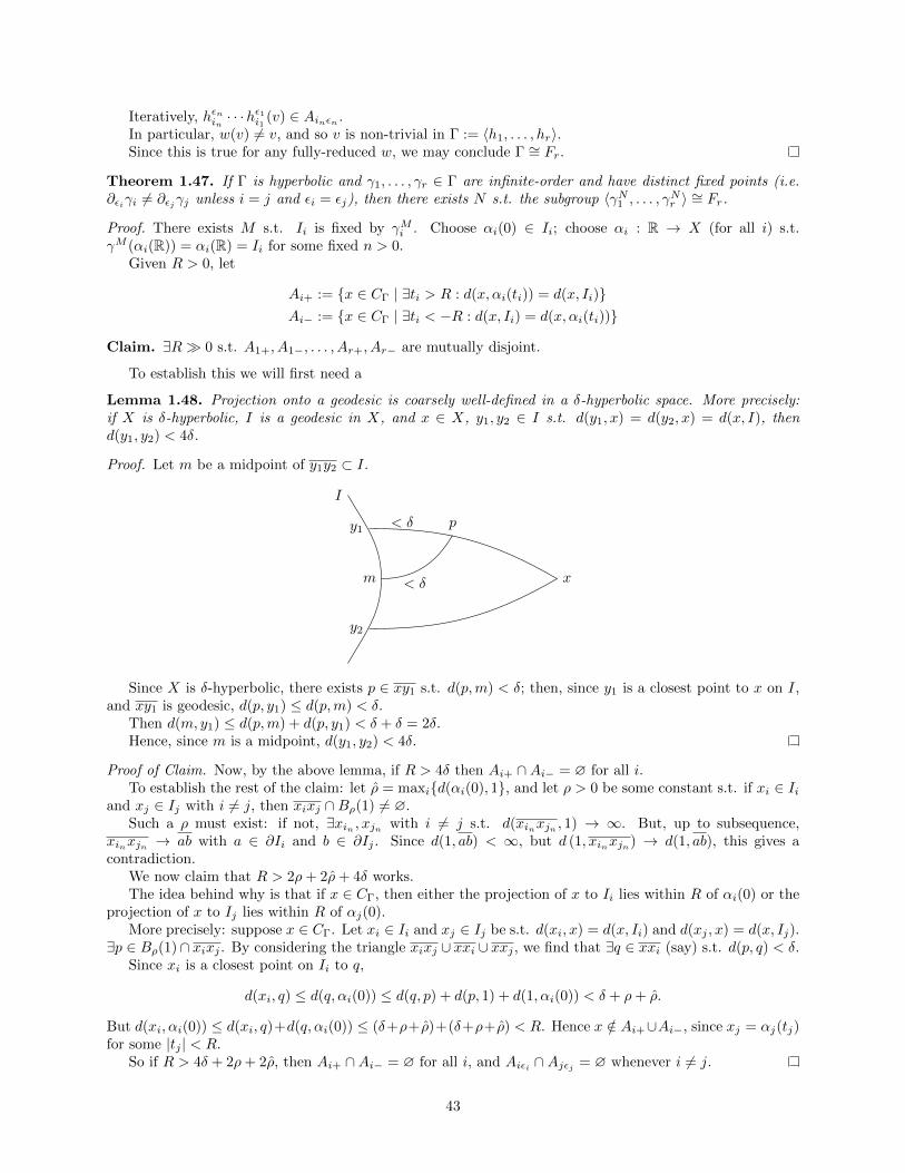
Iteratively, hεnin · · ·hε1i1
(v) ∈ Ainεn .In particular, w(v) 6= v, and so v is non-trivial in Γ := 〈h1, . . . , hr〉.Since this is true for any fully-reduced w, we may conclude Γ ∼= Fr.
Theorem 1.47. If Γ is hyperbolic and γ1, . . . , γr ∈ Γ are infinite-order and have distinct fixed points (i.e.∂εiγi 6= ∂εjγj unless i = j and εi = εj), then there exists N s.t. the subgroup 〈γN1 , . . . , γNr 〉 ∼= Fr.
Proof. There exists M s.t. Ii is fixed by γMi . Choose αi(0) ∈ Ii; choose αi : R → X (for all i) s.t.γM (αi(R)) = αi(R) = Ii for some fixed n > 0.
Given R > 0, let
Ai+ := x ∈ CΓ | ∃ti > R : d(x, αi(ti)) = d(x, Ii)Ai− := x ∈ CΓ | ∃ti < −R : d(x, Ii) = d(x, αi(ti))
Claim. ∃R 0 s.t. A1+, A1−, . . . , Ar+, Ar− are mutually disjoint.
To establish this we will first need a
Lemma 1.48. Projection onto a geodesic is coarsely well-defined in a δ-hyperbolic space. More precisely:if X is δ-hyperbolic, I is a geodesic in X, and x ∈ X, y1, y2 ∈ I s.t. d(y1, x) = d(y2, x) = d(x, I), thend(y1, y2) < 4δ.
Proof. Let m be a midpoint of y1y2 ⊂ I.
I
m
y1
x
y2
p< δ
< δ
Since X is δ-hyperbolic, there exists p ∈ xy1 s.t. d(p,m) < δ; then, since y1 is a closest point to x on I,and xy1 is geodesic, d(p, y1) ≤ d(p,m) < δ.
Then d(m, y1) ≤ d(p,m) + d(p, y1) < δ + δ = 2δ.Hence, since m is a midpoint, d(y1, y2) < 4δ.
Proof of Claim. Now, by the above lemma, if R > 4δ then Ai+ ∩Ai− = ∅ for all i.To establish the rest of the claim: let ρ = maxid(αi(0), 1, and let ρ > 0 be some constant s.t. if xi ∈ Ii
and xj ∈ Ij with i 6= j, then xixj ∩Bρ(1) 6= ∅.Such a ρ must exist: if not, ∃xin , xjn with i 6= j s.t. d(xinxjn , 1) → ∞. But, up to subsequence,
xinxjn → ab with a ∈ ∂Ii and b ∈ ∂Ij . Since d(1, ab) < ∞, but d (1, xinxjn) → d(1, ab), this gives acontradiction.
We now claim that R > 2ρ+ 2ρ+ 4δ works.The idea behind why is that if x ∈ CΓ, then either the projection of x to Ii lies within R of αi(0) or the
projection of x to Ij lies within R of αj(0).More precisely: suppose x ∈ CΓ. Let xi ∈ Ii and xj ∈ Ij be s.t. d(xi, x) = d(x, Ii) and d(xj , x) = d(x, Ij).
∃p ∈ Bρ(1)∩ xixj . By considering the triangle xixj ∪ xxi ∪ xxj , we find that ∃q ∈ xxi (say) s.t. d(p, q) < δ.Since xi is a closest point on Ii to q,
d(xi, q) ≤ d(q, αi(0)) ≤ d(q, p) + d(p, 1) + d(1, αi(0)) < δ + ρ+ ρ.
But d(xi, αi(0)) ≤ d(xi, q)+d(q, αi(0)) ≤ (δ+ρ+ ρ)+(δ+ρ+ ρ) < R. Hence x /∈ Ai+∪Ai−, since xj = αj(tj)for some |tj | < R.
So if R > 4δ + 2ρ+ 2ρ, then Ai+ ∩Ai− = ∅ for all i, and Aiεi ∩Ajεj = ∅ whenever i 6= j.
43

Ii
Ij
Figure 36: Why ρ must exist, a schematic illustration
x
xi
xj
pq
Figure 37: Why R > 2ρ+ 2ρ+ 4δ works, a schematic illustration.
Now choose n s.t. nτ(γmi ) > 8R for all i.Suppose x ∈ CΓ −Ai−. Then if xi ∈ Ii and d(x, xi) = d(x, Ii), then xi = αi(t) for t ≥ −R;
d(γnMi (x), Ii) = d(αi(t+ nMτ(γi)))
implies αi(t+ nMτ(γi)) is a projection of γnMi (x).By assumption, t+nMτ(γi) > 7R, so any projection of γnMi (x) onto Ii has coordinate ≥ 7R− 4δ > 6R,
and so γnMi (x) ∈ Ai+. (Or, roughly speaking, the projection onto Ii is not just coarsely well-defined, butalso coarsely equivariant.) So if N = nM , then γNi (CΓ −Ai−) ⊂ Ai+ for all i.
Similarly, γ−Ni (CΓ −Ai+) ⊂ Ai− for all i.By Lemma 1.46 (ping-pong), 〈γN1 , . . . , γNr 〉 ∼= Fr.
Recall the Tits Alternative
Theorem 1.49. If Γ is hyperbolic, then OOTFH:
(a) Γ is finite,
(b) Γ is virtually infinite cyclic, or
(c) Γ contains a [quasi-convex] subgroup isomorphic to F2.
44

Recall: if we let β(n) = #γ ∈ Γ | `(γ) ≤ n, then [we showed that] β(n) is well-defined up to quasi-equivalence.
In case (a) above, β is bounded; in case (b), β is linear; in case (c), β is exponential.
Theorem 1.50 (Gromov, Cannon). B(x) =∑n β(n)xn is a rational function for Γ hyperbolic (for any
choice of generators of Γ.)
Then, combined with the discussion above, we have
Corollary. If Γ is quasi-isometric to Z, then Γ is virtually cyclic.
Proof. Quasi-isometric groups have quasi-equivalent growth functions β.
Proof of Tits Alternative. (1) If Γ is infinite, then Γ has an infinite-order element (this part we will notprove unless we develop more machinery about ∂X.)
(2) If Γ contains two infinite-order elements α, β with distinct fixed points, then it contains F2 (from Theorem1.47.)
(3) If [there exist infinite-order elements and] all infinite-order elements share ≥ 1 fixed point/s, then Γ isvirtually cyclic.
Claim. If α, β infinite-order share one fixed point, then they share both fixed points.
Figure 38: tl;dr: the situation pictured leads to nondiscreteness.
Proof. Choose M s.t. αM and βM have invariant axes A and B. WMA M = 1. WLOG ∂+α = ∂+β.Parametrize A,B by a : R→ CΓ, b : R→ CΓ (resp.) s.t. α(a(t)) = a(t+ τ(α)) and β(b(t)) = b(t+ τ(β)).
Let R = d(a(0), b(0)); then d(a(t), b(t)) < R + 3δ for all t > 0. (Since ideal triangles in a δ-hyperbolicspace are 3δ-thin, we have s < R+t+3δ and t < R+s+3δ. Combining the two, obtain |s−t| < R+3δ.)
Then, for all n > 0,
d(α−nβαn(a(0)), b(τ(β))) = d (β(a(nτ(α))), αn(b(τ(β)))
≤ d (β(a(nτ(α))), αn(a(τ(β)))) + (R+ 3δ)
= d (β(a(nτ(α))), a(τ(β) + nτ(α))) + (R+ 3δ)
≤ d (β(b(nτ(α))), a(τ(β) + nτ(α))) + 2(R+ 3δ)
= d (b(nτ(α) + τ(b)), a(τ(β) + nτ(α))) + 2(R+ 3δ)
≤ 3(R+ 3δ)
Therefore there are ∃#B3(R+3δ)(1) choices for α−nβαn. Hence ∃n1 6= n2 s.t. α−n1βαn1 = α−n2βαn2 ,i.e. αn2−n1βαn1−n2 = β, i.e. αn2−n1 ∈ Z(〈β〉), which is virtually cyclic; so some power of α is the samepower of β, i.e. ∂±α = ∂±β.
Claim. If all infinite-order elements of Γ share both of their fixed points, then Γ is virtually cyclic.
45

Proof. Let a, b be the fixed points of all the infinite-order elements of Γ.
Let S be the set of special geodesics. S is finite. Let α ∈ Γ have infinite order.
If γ ∈ Γ, then γαγ−1 has infinite order and ∂±(γαγ−1) = ∂±α = γ(a), γ(b).So ∃ subgroup Γ0 of index ≤ 2 s.t. γ(a) = a and γ(b) = b for all γ ∈ Γ0, i.e. −γ(S) = S.
Let φ : Γ0 → ΣS (the permutation group on S), and Γ1 = ker(φ) which has finite index in Γ0.
Now Γ1 acts freely and properly on I ∈ S, and hence Γ1∼= Z; alternatively, we may say that if α ∈ Γ1
has infinite order, then Γ1 ⊂ Z(〈α〉) and so Γ1 is virtually cyclic.
1.13 The Rips Complex
Theorem 1.51 (Rips). If Γ is hyperbolic, it acts on a simplicial complex P s.t.
1. P is finite-dimensional, contractible, and locally finite.
2. Γ acts simplicially and co-compactly with finite stabilizers.
3. Γ acts freely and transitively on P 0.
Corollary. Γ torsion-free =⇒ P/Γ is a finite K(π, 1).
Corollary. For all large enough n, Hn(Γ,Q) is trivial.This proof of this one uses spectral sequences.
Proof. Consider the Cayley graph CΓ with R > 0. Then PR(CΓ) is the simplicial complex s.t. PR(CΓ)0 =Γ and γ0, . . . , γn span an n-simplex if diamCΓ
(γ0, . . . , γn) ≤ R. PR(CΓ) is locally finite and finite-dimensional since BCΓ
(R, 1) is finite.#BCΓ
(R, 1) = #BCΓ(R, γ) for all γ ∈ Γ. γ(γ0, . . . , γn) = (γγ0, . . . , γγn) determines a simplicial action
on PR(CΓ).Since Γ acts freely on Γ, it acts freely on PR(CΓ)0.The action of Γ is co-compact since it acts transitively on PR(CΓ)0 and PR(CΓ)0 is locally finite.γ stabilizes a simplex γ0, . . . , γn iff it permutes the vertices, so the stabilizer of a n-simplex has order
≤ (n+ 1)!If R > 1, PR(CΓ) = CΓ,Y , where Y = γ ∈ Γ | dCΓ
(1, γ) ≤ R; in particular, PR(CΓ) is connected (i.e.has trivial π0.)
The proof of the theorem then reduces to the following
Claim. If R > 4δ + 6 then PR(CΓ) is contractible.
To establish this last result, it suffices to show that πn(P ) is trivial for all n > 0, i.e. any map of an-sphere into P can be contracted to a point.
Any image of a sphere lies in a finite subcomplex, so it suffices to show any subcomplex L can becontracted to a point in P .
Case 1: diam(L) ≤ R.In this case, the vertices in L0 have diameter ≤ R, so the vertices of L0 span a simplex in P ; hence L ⊂
some simplex of P , and so L can be contracted to a point.Case 2: diam(L) > R.Fix v0 ∈ L0, and choose w ∈ L0 s.t. dCΓ(v0, w) is maximal (over all w ∈ L0), so dCΓ(v0, w) > R.Choose a vertex y ∈ v0w s.t. d(y, w) ∈ [R2 ,
R2 + 1].
Claim. If u ∈ L0 with d(u,w) ≤ R, then d(u, y) ≤ R.
Proof. Consider the triangle T with edges v0w, v0u and uw. Notice that `(uw) ≤ R and `(v0u) ≤ `(v0w).
46

u
v0 wy R/2
Since CΓ is δ-hyperbolic, ∃p ∈ uw ∪ v0u s.t. d(y, p) < δ.If p ∈ uw: since d(w, y) ≥ R
2 > 2δ, hence we have d(w, y) > d(p, y), and thus d(u, y) < d(u,w) ≤ R.Otherwise, if p ∈ v0u: if d(u, y) > R, then d(u, p) > R− δ; hence d(v0, w) ≤ d(v0, p) + d(p, y) + d(y, w) ≤
d(v0, p) + δ+ R2 + 1. But d(v0, u) = d(v0, p) +d(p, u) ≥ d(v0, p) +R− δ, since R− δ > R
2 + δ+ 1 by our choiceof R > 4δ + 6. Hence we would have d(v0, u) > d(v0, w), contradicting the maximality of d(v0, w)—hencewe must conclude d(u, y) ≤ R.
Let L′ be obtained from L by replacing every simplex (w, γ1, . . . , γn) by the simplex (y, γ1, . . . , γn). Ourclaim above guarantees that (y, γ1, . . . , γn) is a simplex. One can homotope L to L′ within P by linearlydeforming (w, γ1, . . . , γn) to (y, γ1, . . . , γn) through (w, y, γ1, . . . , γn). This either (a) reduces maxd(v0, w) |w ∈ L0 by ≥ 1, or (b) reduces # w ∈ L0 | d(v, w) maximal, so after finitely many steps we arrive at Ls.t. diam(L) < R and L can be homotoped to L; and then we may apply the arguments of Case 1 above.
1.14 The Mostow Rigidity Theorem
Or, a sketch of a pretty cool result
Theorem 1.52. If M = H3/ΓM and N = H3/ΓN are closed13 hyperbolic 3-manifolds, and f : M → N is ahomotopy equivalence, then ∃ an isometry g : M → N homotopic to f .
Sketch of proof. (1) f : M → N lifts to a quasi-isometry f : H3 → H3 (essentially, using the Milnor-Svarclemma.)
(2) f extends to a quasi-conformal map g : ∂H3 → ∂H3 (recall a quasi-conformal map is a map whichdistorts the conformal structure by a bounded amount.)14
(3) g is differentiable almost everywhere and dg(z) 6= 0 a.e.
(4) Either (“Sullivan”)
Theorem 1.53 (Tukia). If g : C→ C conjugates ΓM to ΓN (both co-compact) and dg(z) 6= 0, then g isconformal (or anti-conformal.)
or (“Mostow”) If g is not conformal, then there exists dg a measurable ΓM -invariant line field (direction
of maximal stretch); now apply the ergodicity of the action of Γ on C× C to show this is impossible.
The proof of (1) proceeds, morally, by noting that f = f∗ which is a quasi-isometry. More precisely,notice that f∗ : ΓM → ΓN is an isomorphism, and so f∗ is a quasi-isometry w.r.t. any word metric; thenf : ΓM (x0)→ ΓN (f(x0)) is a (k, c)-quasi-isometry (for some k, c) by Milnor-Svarc.
WMA f is Lipschitz and let D = diam(M); then f : H3 → H3 is a (k, c+ 2D)-quasi-isometry.
13We may generalize this to finite-volume14Note further that g : ∂H3 → ∂H3 induces a map ∂ΓM → ∂ΓN .
47

For the proof of (2), recall that a homeomorphism g is k-quasiconformal if for all z,
lim supr→0
maxθ(d(g(z), g(z + reiθ)
)minθ (d(g(z), g(z + reiθ))
≤ k
Claim. Let g = f : C→ C. Then g is quasiconformal.
In fact this follows from the slightly more general
Proposition 1.54. Given k, c > 0 ∃L > 1 s.t. if h : H3 → H3 is a (k, c)-quasi-isometry, then h : ∂H3 → ∂H3
is L-quasiconformal.
Proof. The proof uses a key
Lemma 1.55. ∃D > 0 s.t. if L is a geodesic, P is a totally geodesic hyperplane s.t. L ⊥ P , L′ =h(∂+L)h(∂−L) is a geodesic asymptotic to h(L), and πL′ denotes nearest-point projection, onto L′, then
diam(πL′(f(P ))) ≤ D
h~L
zP
Figure 39: Illustration of Lemma 1.55
To reduce our result to this lemma, suppose z ∈ C; let L = z∞ and Pr be a plane in H3 with ∂Pr acircle Sr of radius r about z. Now h(Sr) = h(Pr) ∩ C.
WLOG h(z) = 0, h(∞) =∞, and so (we may assume) L′ is the t-axis.
Now let s = min(πL′(h(Pr))); then πL′(h(Pr)) ⊂ [s, eDs]. Hence h(Pr) ⊂ B(0, eDs)−B(0, s) ⊂ C. Hence
max(d(h(z), h(z + reiθ)
)min (d(h(z), h(z + reiθ))
≤ eDs
s= eD
and so the lim sup of this quantity as r → 0 is also ≤ eD; hence h is now eD-quasiconformal.
Figure 40: Lemma 1.55 implies quasiconformality
48
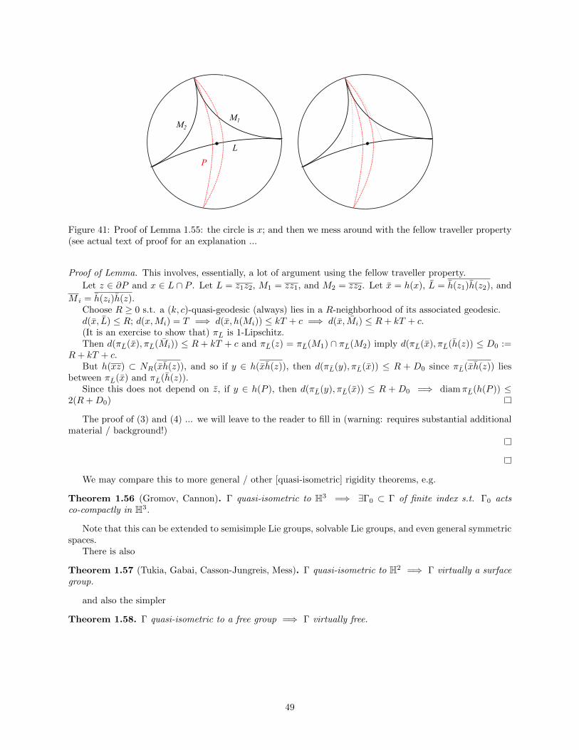
P
M1M2
L
Figure 41: Proof of Lemma 1.55: the circle is x; and then we mess around with the fellow traveller property(see actual text of proof for an explanation ...
Proof of Lemma. This involves, essentially, a lot of argument using the fellow traveller property.
Let z ∈ ∂P and x ∈ L ∩ P . Let L = z1z2, M1 = zz1, and M2 = zz2. Let x = h(x), L = h(z1)h(z2), and
M i = h(zi)h(z).Choose R ≥ 0 s.t. a (k, c)-quasi-geodesic (always) lies in a R-neighborhood of its associated geodesic.d(x, L) ≤ R; d(x,Mi) = T =⇒ d(x, h(Mi)) ≤ kT + c =⇒ d(x, Mi) ≤ R+ kT + c.(It is an exercise to show that) πL is 1-Lipschitz.Then d(πL(x), πL(Mi)) ≤ R + kT + c and πL(z) = πL(M1) ∩ πL(M2) imply d(πL(x), πL(h(z)) ≤ D0 :=
R+ kT + c.But h(xz) ⊂ NR(xh(z)), and so if y ∈ h(xh(z)), then d(πL(y), πL(x)) ≤ R + D0 since πL(xh(z)) lies
between πL(x) and πL(h(z)).Since this does not depend on z, if y ∈ h(P ), then d(πL(y), πL(x)) ≤ R + D0 =⇒ diamπL(h(P )) ≤
2(R+D0)
The proof of (3) and (4) ... we will leave to the reader to fill in (warning: requires substantial additionalmaterial / background!)
We may compare this to more general / other [quasi-isometric] rigidity theorems, e.g.
Theorem 1.56 (Gromov, Cannon). Γ quasi-isometric to H3 =⇒ ∃Γ0 ⊂ Γ of finite index s.t. Γ0 actsco-compactly in H3.
Note that this can be extended to semisimple Lie groups, solvable Lie groups, and even general symmetricspaces.
There is also
Theorem 1.57 (Tukia, Gabai, Casson-Jungreis, Mess). Γ quasi-isometric to H2 =⇒ Γ virtually a surfacegroup.
and also the simpler
Theorem 1.58. Γ quasi-isometric to a free group =⇒ Γ virtually free.
49

2 CAT(0) groups
Let X be a proper geodesic metric space. If ∆ is a geodesic triangle in X, there exists a comparison triangle∆ in Euclidean space E2 with the same side-lengths:
xz
y X
xz
y
in comparison (Euclidean) space
If a, b ∈ ∆, there exist corresponding points a, b ∈ ∆.
Definition 2.1. X is CAT(0) if d(a, b) ≤ d(a, b) for all ∆, a, b ∈ X.
We may think of this as a strengthening of (δ-)hyperbolicity. We may replace E2 in the above with H2
to obtain the definition of CAT(-1) spaces; sometimes we use comparison triangles on the sphere—here weobtain CAT(1) spaces.
Example 2.2. Some examples include
• Euclidean space En
• Trees
• H2
• M a Riemannian manifold with sectional curvature ≤ 0.
Fact. X is uniquely geodesic
Proof. If not, consider the degenerate triangle formed by two geodesics between distinct points x, y ∈ X(and a side of length 0):
x y
z
Some choice of points in this triangle (or the triangle with x, y, z where z is on one of the geodesics, veryclose to x) would violate the CAT(0) condition.
Fact. Local geodesics are global geodesicsi.e. if γ : [0, R]→ X has the property that ∀t ∈ [0, R] ∃ε > 0 s.t. γ|[t−ε,t+ε] is geodesic, then γ is geodesic.
Proof. Let T = t | γ|[0,t] geodesic. T is closed and contains a neighborhood of 0. We now claim that T isalso open: let s = supT and suppose s < R.
50

Then d(γ(s− ε2 ), γ(s+ ε
2 )) = ε, but has to be less than ε in the comparison triangle—contradiction.
Corollary. If X,Y are CAT(0), and f : X → Y is a locally-isometric immersion, then f : X → Y is anisometric embedding.
Fact. X is contractible
Proof. Fix x0 ∈ X. For any x ∈ X, ∃ geodesic γX : [0, rX ] → X s.t. γx(0) = x0 and γx(rx) = x. DefineH : X × [0, 1]→ X by H(X, t) = γx(trx). H is a homotopy from id to the constant map with image x0.
Note that we may define such a map H for any space, but that here we can sue the CAT(0) condition toshow that it is locally Lipschitz / continuous, and so indeed a homotopy as desired.
Definition 2.3. Γ is a CAT(0) group if it acts properly and co-compactly on some CAT(0) space X.
Example 2.4. • Free abelian groups Zn
• Free groups Fn
• Surface groups π1(Σ)
• π1(M) of closed non-positively-curved Riemannian manifolds M
Fact. If X and Y are CAT(0) spaces, then X × Y (with the product metric) is CAT(0).
Corollary. If Γ1 and Γ2 are CAT(0) groups, then Γ1 × Γ2 is CAT(0).
2.1 Isometries of CAT(0) space
Here (and for the rest of this section of the notes) let X be a proper geodesic CAT(0) space.Suppose γ ∈ Isom(X).
Definition 2.5. τ(γ) := infx∈X d(x, γ(x)) is the translation length. min(γ) := x ∈ X | d(x, γ(x)) =τ(γ).
Definition 2.6. γ is
• elliptic if τ(γ) = 0 and min(γ) 6= ∅.
• hyperbolic if τ(γ) > 0 and min(γ) 6= ∅
• parabolic if min(γ) = ∅
It may be shown that any γ ∈ Isom(X) is of one of these three types.
Fact. If γ is hyperbolic, it has an invariant axis A, i.e. a geodesic A s.t. γ(A) = A and γ acts on A bytranslation by τ(γ).
Proof. Define A :=⋃n∈Z γ
n(x0)γn+1(x0) where x0 ∈ min(γ).
· · ·x0 γ(x0)
γ2(x0) γ3(x0)
We only need to observe that A is locally geodesic, and by equivariance it suffices to check this at γ(x0).Suppose not; then we have
m
x0
(x0)
(x0)
(m)
51

Now let m be the midpoint of x0γ(x0); γ(m) will then be the midpoint of γ(x0)γ2(x0). Then
d(m, γ(m)) < d(m, γ(x0)) + d(γ(x0), γ(m)) = τ(γ)
which contradicts that τ(γ) is the minimum translation distance.
Fact. If Γ acts on X properly and co-compactly, then all the elements of Γ are elliptic or hyperbolic
Proof. This follows once we prove that min(γ) 6= ∅.Let x1, . . . , xn be a sequence in X s.t. d(xn, γ(xn))→ τ(γ). Let K ⊂ X be a compact set s.t. Γ ·K = X.For all n, there exists αn ∈ Γ s.t. αn(xn) =: yn ∈ K. Since d(αnγα
−1n (yn), yn) = d(γ(xn), xn) → τ(γ),
we have finitely many choices for αnγα−1n .
Now pass to a subsequence s.t. αnγα−1n = γ and yn → y. Then, since τ(γ) = τ(γ), we have yn → y =⇒
d(γ(yn), yn)→ τ(γ), and so y ∈ min(γ) 6= ∅.But now min(γ) = αn(min(γ)) and hence we may conclude min(γ) 6= ∅.
Corollary. Finite order elements of Γ (as above) have fixed points.
Corollary. If γ ∈ Γ has infinite order, and α ∈ Γ with αγα−1 = γp, then p = ±1.In other words, if H ⊂ Γ is isomorphic to BS(m,n) := 〈a, t | tamt−1 = an〉, then |m| = |n|.
Proof. Since αγα−1 = γp, τ(γp) = τ(γ).Since γ has an invariant axis, τ(γp) = |p|τ(γ) (from the below arguments.)Hence we must have |p| = 1.
Let us close this section by proving some useful facts about nearest-point retraction in CAT(0) spaces(which we need also to complete the above.)
Fact. If X is CAT(0) and C ⊂ X is closed and convex (i.e. if x, y ∈ C, then xy ∈ C), then the nearest-pointretraction π1 : X → C is well-defined and 1-Lipschitz.
Proof. To show that it is well-defined, we look at comparison triangles: if yz ∈ C, ∃t ∈ yz s.t. d(t, x) ≤d(t, x) ≤ d(x, y) = d(x, y).
x
zy
t
To show that it is 1-Lipschitz, for any x, y ∈ X form the (comparison) quadrilateral xyπ1(x)π1(y).
x y
(y)(x)
Figure 42: The [quadrilateral we form the] comparison quadilateral [to].
If the angle α < π2 , then ∃ a point on πC(x)πC(y) closer to x than πC(x), and hence ∃ a point on
πC(x)πC(y) ⊂ C closer to x than πC(x). This is impossible, so α ≥ π2 , and similarly β ≥ π
2 .Since the comparison quadrilateral must be Euclidean, we have
d(πC(x), πC(y)) = d(πC(x), πC(y)) ≤ d(x, y) = d(x, y).
52
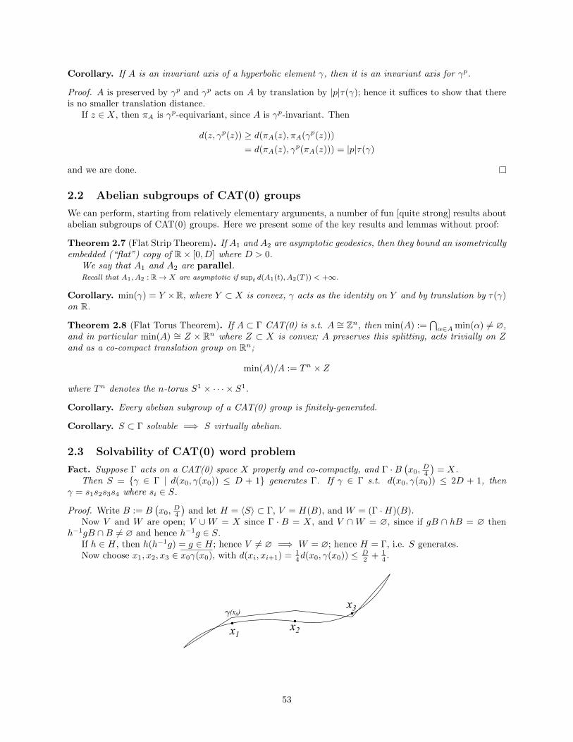
Corollary. If A is an invariant axis of a hyperbolic element γ, then it is an invariant axis for γp.
Proof. A is preserved by γp and γp acts on A by translation by |p|τ(γ); hence it suffices to show that thereis no smaller translation distance.
If z ∈ X, then πA is γp-equivariant, since A is γp-invariant. Then
d(z, γp(z)) ≥ d(πA(z), πA(γp(z)))
= d(πA(z), γp(πA(z))) = |p|τ(γ)
and we are done.
2.2 Abelian subgroups of CAT(0) groups
We can perform, starting from relatively elementary arguments, a number of fun [quite strong] results aboutabelian subgroups of CAT(0) groups. Here we present some of the key results and lemmas without proof:
Theorem 2.7 (Flat Strip Theorem). If A1 and A2 are asymptotic geodesics, then they bound an isometricallyembedded (“flat”) copy of R× [0, D] where D > 0.
We say that A1 and A2 are parallel.Recall that A1, A2 : R→ X are asymptotic if supt d(A1(t), A2(T )) < +∞.
Corollary. min(γ) = Y ×R, where Y ⊂ X is convex, γ acts as the identity on Y and by translation by τ(γ)on R.
Theorem 2.8 (Flat Torus Theorem). If A ⊂ Γ CAT(0) is s.t. A ∼= Zn, then min(A) :=⋂α∈A min(α) 6= ∅,
and in particular min(A) ∼= Z × Rn where Z ⊂ X is convex; A preserves this splitting, acts trivially on Zand as a co-compact translation group on Rn;
min(A)/A := Tn × Z
where Tn denotes the n-torus S1 × · · · × S1.
Corollary. Every abelian subgroup of a CAT(0) group is finitely-generated.
Corollary. S ⊂ Γ solvable =⇒ S virtually abelian.
2.3 Solvability of CAT(0) word problem
Fact. Suppose Γ acts on a CAT(0) space X properly and co-compactly, and Γ ·B(x0,
D4
)= X.
Then S = γ ∈ Γ | d(x0, γ(x0)) ≤ D + 1 generates Γ. If γ ∈ Γ s.t. d(x0, γ(x0)) ≤ 2D + 1, thenγ = s1s2s3s4 where si ∈ S.
Proof. Write B := B(x0,
D4
)and let H = 〈S〉 ⊂ Γ, V = H(B), and W = (Γ ·H)(B).
Now V and W are open; V ∪W = X since Γ · B = X, and V ∩W = ∅, since if gB ∩ hB = ∅ thenh−1gB ∩B 6= ∅ and hence h−1g ∈ S.
If h ∈ H, then h(h−1g) = g ∈ H; hence V 6= ∅ =⇒ W = ∅; hence H = Γ, i.e. S generates.Now choose x1, x2, x3 ∈ x0γ(x0), with d(xi, xi+1) = 1
4d(x0, γ(x0)) ≤ D2 + 1
4 .
x1 x2
x3(x0)
53
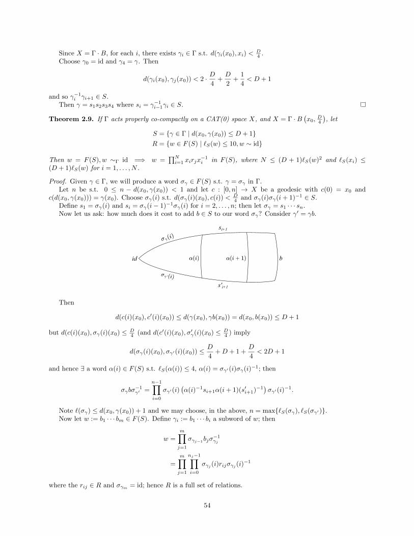
Since X = Γ ·B, for each i, there exists γi ∈ Γ s.t. d(γi(x0), xi) <D4 .
Choose γ0 = id and γ4 = γ. Then
d(γi(x0), γj(x0)) < 2 · D4
+D
2+
1
4< D + 1
and so γ−1i γi+1 ∈ S.
Then γ = s1s2s3s4 where si = γ−1i−1γi ∈ S.
Theorem 2.9. If Γ acts properly co-compactly on a CAT(0) space X, and X = Γ ·B(x0,
D4
), let
S = γ ∈ Γ | d(x0, γ(x0)) ≤ D + 1R = w ∈ F (S) | `S(w) ≤ 10, w ∼ id
Then w = F (S), w ∼Γ id =⇒ w =∏Ni=1 xirjx
−1i in F (S), where N ≤ (D + 1)`S(w)2 and `S(xi) ≤
(D + 1)`S(w) for i = 1, . . . , N .
Proof. Given γ ∈ Γ, we will produce a word σγ ∈ F (S) s.t. γ = σγ in Γ.Let n be s.t. 0 ≤ n − d(x0, γ(x0)) < 1 and let c : [0, n] → X be a geodesic with c(0) = x0 and
c(d(x0, γ(x0))) = γ(x0). Choose σγ(i) s.t. d(σγ(i)(x0), c(i)) < D4 and σγ(i)σγ(i+ 1)−1 ∈ S.
Define s1 = σγ(i) and si = σγ(i− 1)−1σγ(i) for i = 2, . . . , n; then let σγ = s1 · · · sn.Now let us ask: how much does it cost to add b ∈ S to our word σγ? Consider γ′ = γb.
id b
si+1
s'i+1
Then
d(c(i)(x0), c′(i)(x0)) ≤ d(γ(x0), γb(x0)) = d(x0, b(x0)) ≤ D + 1
but d(c(i)(x0), σγ(i)(x0) ≤ D4 (and d(c′(i)(x0), σ′γ(i)(x0) ≤ D
4 ) imply
d(σγ(i)(x0), σγ′(i)(x0)) ≤ D
4+D + 1 +
D
4< 2D + 1
and hence ∃ a word α(i) ∈ F (S) s.t. `S(α(i)) ≤ 4, α(i) = σγ′(i)σγ(i)−1; then
σγbσ−1γ′ =
n−1∏i=0
σγ′(i)(α(i)−1si+1α(i+ 1)(s′i+1)−1
)σγ′(i)
−1.
Note `(σγ) ≤ d(x0, γ(x0)) + 1 and we may choose, in the above, n = max`S(σγ), `S(σγ′).Now let w := b1 · · · bm ∈ F (S). Define γi := b1 · · · bi a subword of w; then
w =
m∏j=1
σγj−1bjσ−1γj
=
m∏j=1
nj−1∏i=0
σγj (i)rijσγj (i)−1
where the rij ∈ R and σγm = id; hence R is a full set of relations.
54

Moreover, the number of relations used N is given by n1 + · · · + nm. Note that we have nj ≤ `S(γj) ≤j(D + 1) + 1, and `S
(σγj (i)
)≤ i(D + 1) + 1, and so
N = n1 + · · ·+ nm ≤m∑j=1
j(D + 1) + 1
≤ (D + 1)
m∑j=1
j
+m
= (D + 1)
(m+ 1
2
)+m
≤ (D + 1)m2 = (D + 1)`S(w)2
and `S(σj(i)) ≤ i(D + 1) + 1 ≤ m(D + 1) = `S(w)(D + 1) for all i.
Corollary. If Γ is a CAT(0) group, then define S and R as above; then Γ = 〈S;R〉 is finitely-presented, hassolvable word problem, and has a quadratic Dehn function.
2.4 Cube Complexes
Definition 2.10. A cube complex is a space constructed from unit Euclidean cubes by identifying facesby isometries
Figure 43: A cube complex (black / grey) and a link of a vertex (blue).
We will always assume that our cube complexes are locally finite.
Definition 2.11. The link of a vertex v in a cube complex K, denoted Lk(K, v), is a simplicial complexs.t. a neighborhood of v is isometric to a neighborhood of the cone point in the cone on Lk(K, v).
Cube complexes need not be CAT(0): consider, for instance
Figure 44: (The pictured red triangle on the left = filled yellow in the middle) ∆ is thicker than thecomparison triangle ∆ ⊂ ∆; the right diagram is a different example of a non-CAT(0) cube complex.
We can however find relatively simple / concise conditions s.t. cube complexes satisfying these conditionswill be CAT(0):
We say that K is locally CAT(0) if ∀x ∈ K ∃ a convex neighborhood U of x in K s.t. all triangles inU satisfy the CAT(0) criterion; we also say that K has non-positive curvature.
55

Theorem 2.12 (Cartan-Hadamard). K simply-connected, complete, locally CAT(0) =⇒ K CAT(0).
Definition 2.13. A simplicial complex K is a flag complex if whenever w0, . . . , wn are vertices in K with[wi, wj ] an edge in K for all 0 ≤ i 6= j ≤ n, [w0, . . . , wn] span an n-simplex in K.
Theorem 2.14 (Gromov’s Link Criterion). K locally CAT(0) ⇐⇒ for all vertices v ∈ K, Lk(K, v) is aflag complex.
In 2 dimensions this rules out (for instance) the things we see in Figure 44.The advantage of this criterion is that it is “incredibly checkable.”
Here is one case where we can use Gromov’s Link Criterion (together with Cartan-Hadamard) to showthat a space is CAT(0). Recall the definition of a Right-Angled Artin Group (RAAG): start with G a (finite)graph. Form the group Γ = AG = 〈G0 | [v, w] = 1 ⇐⇒ [v, w] ∈ G1〉.
Fact. RAAGs are CAT(0).
Proof. We will build a locally CAT(0) cube complex K (the Salvetti complex) s.t. π1(K) = AG; then wemay consider the action of AG on K (which is CAT(0) by Cartan-Hadamard.)
We construct K as follows: first let K(1) be the bouquet of circles (with one circle for each vertex of G),i.e. K(0) consists of a single point and K(1)“ =′′ G(0).
Whenever vi, vj are joined by an edge in G, append the square with boundary vivjv−1i v−1
j to K.
Figure 45: A graph for a RAAG (left) and its associated Salvetti complex (right.)
By construction, π1(K) = AG; now make K a flag complex (if v0, . . . , vm ∈ G(0) are s.t. vi, vj are joinedby an edge for all i 6= j, then glue in a n-cube.)
The resulting complex has all Lk(K, v) flag complexes, and hence is CAT(0) by Gromov’s Link Criterion.
Examples 2.15. • If G consists of four vertices and two disjoint edges, then Γ = AG ∼= Z2 ∗ Z2, theSalvetti complex K = S(Γ) is a wedge of two (2-)tori, and the link of the join vertex v in K consistsof two squares joined at a point.
• If G is a triangle, then Γ = AG ∼= Z3, K = S(Γ) is a 3-torus, and the link of any vertex in K ishomeomorphic to a 2-sphere.
2.5 Cartan-Hadamard
Let us prove the Cartan-Hadamard Theorem. We will do so in slightly more generality:
Definition 2.16. X is CAT(k) if every geodesic triangle ∆ in X (of perimeter < 2π√k
if k > 0) is at least
as thin as the comparison triangle ∆ in M2k (the unique simply-connected Riemannian manifold of constant
curvature k.)
Definition 2.17. X is locally CAT(k) if for all x ∈ X there exists a convex neighborhood Ux 3 x s.t.every triangle in Ux satisfies the CAT(k) condition.
We sometimes also say that X has curvature ≤ k.
56

Lemma 2.18. If (a0, b, c0) and (a1, b, c1) are geodesic triangles in X both satisfying the CAT(k) conditionand c0 ∪ c1 is a geodesic in X, then (a0, a1, c0 ∪ c1) is CAT(k).
C
B0 B1A
a0 a1
b
c0 c1
Proof. Let ∆1 = (a1, b, c1) and ∆0 = (a0, b, c0), and consider ∆0 ∪b ∆1.
A
a0 a1b
c0 c1
Claim. The internal angle of ∆0 ∪b ∆1 at A is ≥ π.
Proof. If not, pick p0, p1 near A. We know that, since c0∪c1 is geodesic in X, d(p0, p1) = d(p0, A)+d(A, p1) =d(p0, A) + d(A, p1) > d(p0, p1).
On the other hand, by the CAT(k) condition in each triangle we have d(p0, p1) ≥ d(p0, p1). Contradiction.
And now
A
a0 a1
c0 c1
p0 p1
Corollary. If X1 and X2 are CAT(k) spaces, Ai ⊂ Xi (i = 1, 2) are convex subsets, and we have anisometry j : A1 → A2, then X1 ∪j X2 is also CAT(k).
Sketch of proof. Quite literally:
X1
X2X1 = X2
Theorem 2.19. If X is locally CAT(k), and given any p, q ∈ X s.t. d(p, q) < π√k
there exists a unique
geodesic from p to q (i.e. X is locally geodesic), then X is CAT(k).
57

Proof. Fix p ∈ X and R < π√k
. BR(p) is compact, so there exists ε > 0 s.t. for all x ∈ BR(p), Bε(x) ⊂ Ux,
For all q ∈ BR(p) there exists a unique geodesic cq : [0, 1]→ X parametrized proportional to arc-length.
cq is a continuous function of q (by Arzela-Ascoli) and so ∃δ > 0 s.t. if x, y ∈ BR(p) and d(x, y) < δ thend(cx(t), cy(t)) < ε for all t.
Claim. If d(x, y) < δ, then the triangle (p, x, y) satisfies the CAT(k) condition.
Proof. Choose n s.t. d(cx(in
), cx(i+1n
))< δ and d
(cy(in
), cy(i+1n
))< δ.
p
x
y
δ δ
(p, cx(
1n
), cy(
1n
)) is contained in Bε(p) ⊂ Up, and hence is CAT(k).
Now, inductively (on i) assume (p, cx(in
), cy(in
)is CAT(k). Add first
(cx(in
), cx(i+1n
), cy(in
))and
then(cx(i+1n
), cx(in
), cy(i+1n
)), each of which is CAT(k); the union is CAT(k) by Lemma 2.18.
Claim. If x, y ∈ BR(p) then the triangle (p, x, y) is CAT(k).
Proof. Once again, we glue inductively using our Lemma 2.18:
x
y
< δ< δ< δ< δ< δ< δ< δ< δ
< δ
< δ
(This construction is sometimes known as Alexandrov’s patchwork.)
Proposition 2.20. X simply-connected and locally CAT(0) imply X locally uniquely geodesic.
Proof. Given c : [0, 1] → X a rectifiable path joining x to y parametrized proportional to arc-length, letR = `(c). Choose ε = 1
n > 0 s.t. if x ∈ BR(p), Bε(x) ⊂ Ux.First replace each c|[ in , i+1
n ] by a geodesic segment (straighten piecewise) and reparametrize by arc-length
to get c′; then D(c) is obtained from c′ by replacing each c′([
2i+12n , 2i+3
2n
])with a geodesic segment.
Figure 46: Birkhoff curve shortening, a schematic representation
Claim. Dm(c)→ c∞, a geodesic joining x to y, up to subsequence
Ideas behind proof. Arzela-Ascoli and some sort of energy minimization.
58

If c0, c1 are distinct geodesics, let H = cs be an isotopy by rectifiable curves from c0 to c1. Dn(cs)→ csis a family of geodesics interpolating between c0 and c1. Now d(c0(t), cs(t)) < ε (for all s > 0) implies ourspace is locally convex, and hence (by compactness of [0, 1]) globally convex.
Then we may use the argument that appeared much early for why CAT(0) spaces are uniquely geodesic.
Note that this Proposition, together with the preceding Theorem, together imply the Cartan-Hadamardtheorem.
2.6 Gromov’s link criterion
Theorem 2.21. If K is an Euclidean cube complex, then K is locally CAT(0) if lk(K,x) is CAT(1) for allvertices v.
(Note that this implies K is CAT(0) by Cartan-Hadamard.)
Proof. If p lies in the interior of a cube, one is clearly locally CAT(0) at p (i.e. some neighborhood of p isCAT(0).)
If p lies on a face but is not a vertex: if v is a vertex of that face and U is a neighborhood of v, then ∃V a neighborhood of p which isometrically embeds in U ; hence we can reduce to the case where p = v is avertex.
Let U0 = int(C1∪· · ·∪Cn), where the Ci are the cubes with v as a vertex. By dividing cubes into smallercubes, WMA v is only one of the vertices of each Ci.
If q ∈ U0, ∃ unique geodesic segment γq joining v to q; let r : U0 → lk(K, v) be the projection map.Metrize lk(K, v) as a union of all-right spherical simplices, i.e. if p, q ∈ Ci, d(r(p), r(q)) = ∠(γp, γq).Consider a geodesic α : [0, 1] → X lying in U0 which does not pass through p = v. Also assume r α is
not constant. Consider the partition Pα = t0 = 0 < t1 < t2 < · · · < tn+1 = 1 s.t. α([ti, ti+1]) ⊂ Cj(i) andj(i) 6= j(i+ 1): we may think of this as “understanding our geodesic cube-by-cube.”
Consider the triangles ⊂ Cj(i) and glue the comparison triangles Γi together in E2.The total angle at v is ≤ π, since otherwise γα(0) ∪ γα(1) is shorter than α, which contradicts α geodesic.Now the total angle at v is equal to `(r α); r α must be geodesic, or we could use the geodesic joining
r(α(0)) to r(α(1)) to construct a shorter path joining α(0) to α(1).Notice that ∃ε > 0 s.t. Bε(x) is convex, since if ε is small, any geodesic joining points in Bε(x) lies in U0,
and so has the form above, and in this picture distance to x is locally convex, hence convex.
Claim. If (a, b, c) is a geodesic triangle in Bε(x), then it satisfies the CAT(0) inequality.
Proof. Case 1: Suppose our triangle passes through p. WLOG p ∈ a. (γB , c, γA) is CAT(0) since itscomparison triangle pathwise-isometrically embeds; in particular ∃ a 1-Lipschitz map of the comparisontriangle into K.
Similarly (γC , b, γA) is CAT(0). By Lemma 2.18, (a, b, c) is CAT(0).
C A
B
a
γA
γC
γB
c
b
Case 2: d(r(A), r(B)) + d(r(B), r(C)) + d(r(C), r(A)) < 2π (equivalently, r(a, b, c) is a triangle withperimeter < 2π.)
In this case the CAT(1) condition will come into play straight away: make a comparison tetrahedron inE3:
59
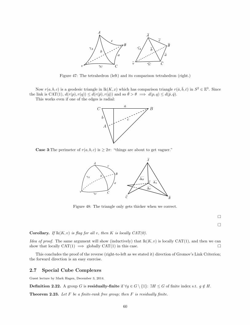
v
A
C
Bc
ba
A
v
b
C
a
c
B
Figure 47: The tetrahedron (left) and its comparison tetrahedron (right.)
Now r(a, b, c) is a geodesic triangle in lk(K,x) which has comparison triangle r(a, b, c) in S2 ∈ E3. Sincethe link is CAT(1), d(r(p), r(q)) ≤ d(r(p), r(q)) and so θ > θ =⇒ d(p, q) ≤ d(p, q).
This works even if one of the edges is radial:
C B
A
a
b c
Case 3:The perimeter of r(a, b, c) is ≥ 2π: “things are about to get vaguer.”
v
A
C
B
c
b
a
A
v
C B
Figure 48: The triangle only gets thicker when we correct.
Corollary. If lk(K, v) is flag for all v, then K is locally CAT(0).
Idea of proof. The same argument will show (inductively) that lk(K, v) is locally CAT(1), and then we canshow that locally CAT(1) =⇒ globally CAT(1) in this case.
This concludes the proof of the reverse (right-to-left as we stated it) direction of Gromov’s Link Criterion;the forward direction is an easy exercise.
2.7 Special Cube Complexes
Guest lecture by Mark Hagen, December 3, 2014.
Definition 2.22. A group G is residually-finite if ∀g ∈ G \ 1: ∃H ≤ G of finite index s.t. g /∈ H.
Theorem 2.23. Let F be a finite-rank free group; then F is residually finite.
60

Remark. SLn(Z) is residually finite, and so RAAGs are residually finite since (by a result of Davis-Januskiewicz) any RAAG embeds into some SLn(Z).
Proof. Let B be a wedge of finitely many circles with π1(B) = F . Choose g ∈ F \ 1 and an edge-pathγ : [0, n]→ B representing g; we require γ to be locally injective.
Figure 49: Given a locally-injective edge-path γ (solid arrowed lines), we can canonically complete it (dashedlines) to a covering space of B.
Make a cover B → B s.t. deg(B → B) < ∞ and the lift of γ at basepoint is not closed—then g /∈π1(B) → π1(B).
Remark. (1) It didn’t matter that the domain of γ was an interval.
Theorem 2.24. If B is a wedge of circles, Γ a finite graph, ϕ : Γ → B an immersion (i.e. a locally-injective graph homomorphism), then ∃ a finite cover B → B and an embedding ϕ : Γ→ B s.t.
B B
Γ
ϕϕ
(2) On the other hand, ∃ CAT(0) groups with no proper finite-index subgroups (see examples by Burger-Mozes and Wise.)
Definition 2.25. Let X and Y be non-positively-curved cube complexes. The combinatorial map15 f :X → Y is a local isometry if
(1) f is locally injective, and
(2) if e1, . . . , en are 1-cubes of X with a common 0-cube and f(e1), . . . , f(en) are 1-cubes of Y which spanan n-cube C of Y , then ∃ n-cube C ′ of X spanned by e1, . . . , en with f(C ′) = C.
Figure 50: If the blue edges map to the red edges, and there’s a grey cube in the target space, there’s acorresponding yellow cube in the domain which maps to the grey cube.
Definition 2.26 (Haglund-Wise 2008). A cube complex X is special if ∃ a simplicial graph Γ and a localisometry X → SΓ, where SΓ denotes the Salvetti complex of AΓ.
Exercise. Basepoint-preserving local isometries induce monomorphisms on π1.
Now let’s talk about why it’s good to be special.
15k-cubes go to k-cubes, and the interiors map isometrically.
61

Figure 51: Examples of non-special (left) and special (right) cube complexes.
Theorem 2.27 (Canonical Completion and Retraction). Let X be a special cube complex, and let Y be acompact cube complex and φ : Y → X a local isometry. Then ∃ a finite cover X → X and an embedding
φ : Y → X s.t.X X
Y
φφ and ∃ a retraction r : X → im(φ).
We may also define specialness in terms of hyperplanes (in fact this was how special cube complexes wereoriginally defined): for each cube C = [−1, 1]n in our cube complex, a midcube in C is a subspace made byrestricting one of the dimensions to 0. The hyperplanes are then built “by radiating out the midcubes asfar as possible.”
Figure 52: The red, blue, and green are hyperplanes.
If X is a non-positively-curved cube complex, let Γ be the graph whose vertex set is the set of hyperplanes,and edge set is given by E(Γ) := (H1, H2) | H1 ∩H2 6= ∅.
Define φ : X → SΓ as follows: for x ∈ X(0), set φ(x) = ∗ ∈ S(0)Γ ; if e is a 1-cube of X, ∃ hyperplane
He intersecting e. Let E be the 1-cube of SΓ labelled by He and send the interior of e isometrically to theinterior of E (this can be done if the hyperplanes of X are 2-sided.
φ is a local isometry, provided
(1) hyperplanes in X are embedded
(2) no self-osculations (see above)
(3) hyperplanes are 2-sided
(4) no inter-osculations (see above.)
62

Figure 53: The four hyperplane pathologies (from left to right): non-embedded hyperplanes, one-sidedhyperplanes, self-osculations, and inter-osculations. Illustration taken from Haglund-Wise.
2.8 A mad dash for the flat torus theorem
Lemma 2.28 (Flat Triangles Lemma). If ∆ = (p, q, r) is a geodesic triangle in a CAT(0) space X and∠ppq, pr = ∠ppq, pr, then p, q, r spans a Euclidean 2-simplex isometric to the 2-simplex D in E2 spanned by∆.
Proof. (1) If s ∈ qr, then d(p, s) = d(p, s).
(See diagrams for Theorem 2.19.)
We observed earlier that α1 + α2 ≥ π =⇒ α1 + α2 ≥ π.
Claim. ¯θ1 + ¯θ2 ≤ θ.Since d(¯p, ¯s) = d(p, s) ≤ d(p, s), we have θi = θi for i = 1, 2 and so α1 + α2 = π; thus ∆1 ∪ ∆2 = ∆, andhence d(p, s) = d(p, s.
(2) Construct a ruled surface D =⋃s∈qr ps.
(See diagrams for Theorem 2.19, particularly the second one for Alexandrov’s patchwork.)
j : D → D takes ps to ps, is an isometry along each ps.
Claim. If xi ∈ psi for i = 1, 2, then d(j(x1), j(x2)) = d(x1, x2).
By the same argument, as above, δ1 = δ1 and so on, and we obtain our claim about distance.
Lemma 2.29 (Flat Quadrilateral Lemma). If (p, q, r, s) span a quadrilateral in X and θp+θq+θr+θs ≥ 2π,then θp + θq + θr + θs = 2π and (p, q, r, s) span a flat filled-in quadrilateral in X
Proof. Apply the Flat Triangle Lemma twice
flat
flatgluing is flat
Figure 54: Arguing as in the Flat Triangle Lemma, each triangle is flat; and the gluing is also flat.
Theorem 2.30 (Flat Strip Theorem). If γ1, γ2 : R→ X are asymptotic geodesics (i.e. supt∈R d(γ1(t), γ2(t)) <+∞), then γ1, γ2 span a flat strip isometric to [0, D]× R ⊂ E2 for some D > 0 (i.e. γ1, γ2 are parallel in aEuclidean sense.)
63
Idea of proof. Look at projections πi : X → γi(R) for i = 1, 2. As nearest-point retractions, these are1-Lipschitz.
WLOG π1(γ2(0)) = γ1(0); let D = d(γ1(0), γ2(0)).d(γ1(t), γ2(t)) is locally convex as a function of t, hence convex, and is bounded non-negative; hence it is
constant. So d(γ1(t), γ2(t)) = D for all t. Similarly, d(γ1(t), γ2(t+ a)) is convex for all a ∈ R.Hence we may infer that all angles are ≥ π
2 , since γ1(0) is the closest point on γ1(R) to γ2(0), etc. Bythe Flat Quadrilateral Lemma, (γ1(0), γ2(0), γ2(t), γ1(t)) span a flat quadrilateral for all t; we can now passto the limit t→ ±∞ to obtain the desired result.
Theorem 2.31 (Decomposition Theorem). If X is CAT(0), γ1 ⊂ X is a geodesic, and Xγ1:= γ(R) ⊂
γ parallel to γ1, then Xγ1= X0
γ1× R, where X0
γ1is a convex subset of X.
Proof. Since every pair of geodesics in Xγ spans a flat strip, Xγ is convex. Consider π1 : Xγ1 → γ1(R) andlet X0
γ1= π−1
1 (0).If x ∈ X0
γ1, ∃γx : R→ X parallel to γ1 s.t. γx(0) = x.
Define j : X0γ1× R→ XΓ1
by j(x, t) = γx(t). We can check that X0γ1
is convex.
Some facts that now follow about hyperbolic isometries: if X is CAT(0), and γ is a hyperbolic isometry,let Min(γ) = x ∈ X | d(x, γ(x)) = τ(γ). Then
(1) γ has an invariant axis in Min(γ). Moreover, every point in Min(γ) lies on an invariant axis.
(2) All axes are parallel
(3) Min(γ) is convex and homeomorphic to Y × R where Y is convex in X, and the action of γ on the firstfactor is trivial.
(4) α ∈ Z(Γ) =⇒ α(Min(γ)) = Min(γ).
Theorem 2.32 (Flat Torus Theorem). If A ∼= Zn acts on a CAT(0) group Γ properly, then
(1) Min(A) :=⋂α∈A Min(α) 6= ∅, and splits as Y × En.
(2) α ∈ A preserves the splitting and acts by translation on En.
(3) y0 × En/A is a flat torus
“There is also some stuff about the normaliser ... ”
Idea of proof. Induct on the rank of A.In the n = 1 case we obtain the picture of the individual hyperbolic isometry.In general, suppose we have a splitting Y ×En which behaves well for Zn−1 ⊂ Zn. Consider α ∈ A which
acts trivially on En−1; consider the action of α on Y , which splits as Y2×R. Then Min(A) = Y2×E×En−1.
Some consequences of the Flat Torus Theorem: suppose Γ acts on X properly and co-compactly. Then
(1) A ⊂ Γ virtually abelian =⇒ A finitely-generated.
(2) A ⊂ Γ virtually solvable =⇒ A virtually abelian.
(3) If X does not contain a flat 2-plane, then Γ is a hyperbolic group.
64

3 Sketches of student talks
Yubo gave talk on the following
Theorem 3.1. Let f : F → F be an automorphism of a finitely-generated free group. Then the fixed groupFix(f) := α ∈ F | f(α) = α is finitely-generated.
Proof. See e.g. S. M. Gersten, “On Fixed Points of Automorphisms of Finitely Generated Free Groups”(Bulletin of the AMS, Vol. 8 No. 3, May 1983.)
This generalizes to
Theorem 3.2 (Paulin, Cooper). Let Γ be a hyperbolic group and f : Γ→ Γ be a group automorphism. ThenFix(f) is finitely-generated.
This is used to prove (rather than going in the other direction)
Theorem 3.3 (Neumann). Fix(f) is quasiconvex
You gave a talk on Terence Tao’s proof of Gromov’s theorem.Both were somewhat muddled, but hey, student talks.
References
• Alessandro Sisto, Lecture notes on Geometric Group Theory
• Brian Bowditch, A course on geometric group theory
• Karen Vogtmann’s lecture notes for a course in geometric group theory
• Cornelia Drutu and Misha Kapovich, Lectures on Geometric Group Theory
• An excellent published source for much of the material is:
Martin Bridson and Andre Haefliger, Metric Spaces of Non-positive curvature, Springer-Verlag, seechapters III.H and III.Gamma for hyperbolic groups and sections II.1, II.5, II.6, II.7, II.8 and III.Gamma.1for CAT(0) groups.
• Another published source for material on hyperbolic groups is; Sur les groups hyperboliques d’apresMikhael Gromov, Etienne Ghys and Pierre de la Harpe, Birkhauser.
65