genetic algorithm-neural network: feature extraction for bioinformatics...
TRANSCRIPT

GENETIC ALGORITHM-NEURAL NETWORK:
FEATURE EXTRACTION FOR BIOINFORMATICS
DATA
DONG LING TONG
A thesis submitted in partial fulfilment of the
requirements of Bournemouth University for
the degree of Doctor of Philosophy
July 2010

Copyright
This copy of the thesis has been supplied on condition that anyone who consults it is understood to recognise
that its copyright rests with its author and due acknowledgement must always be made of the use of any
material contained in, or derived from, this thesis.
i

Abstract
With the advance of gene expression data in the bioinformatics field, the questions which frequently arise,
for both computer and medical scientists, are which genes are significantly involved in discriminating cancer
classes and which genes are significant with respect to a specific cancer pathology.
Numerous computational analysis models have been developed to identify informative genes from the mi-
croarray data, however, the integrity of the reported genes is still uncertain. This is mainly due to the
misconception of the objectives of microarray study. Furthermore, the application of various preprocess-
ing techniques in the microarray data has jeopardised the quality of the microarray data. As a result, the
integrity of the findings has been compromised by the improper use of techniques and the ill-conceived
objectives of the study.
This research proposes an innovative hybridised model based on genetic algorithms (GAs) and artificial
neural networks (ANNs), to extract the highly differentially expressed genes for a specific cancer pathology.
The proposed method can efficiently extract the informative genes from the original data set and this has
reduced the gene variability errors incurred by the preprocessing techniques.
The novelty of the research comes from two perspectives. Firstly, the research emphasises on extracting
informative features from a high dimensional and highly complex data set, rather than to improve classifi-
cation results. Secondly, the use of ANN to compute the fitness function of GA which is rare in the context
of feature extraction.
Two benchmark microarray data have been taken to research the prominent genes expressed in the tumour
development and the results show that the genes respond to different stages of tumourigenesis (i.e. different
fitness precision levels) which may be useful for early malignancy detection. The extraction ability of the
proposed model is validated based on the expected results in the synthetic data sets. In addition, two
bioassay data have been used to examine the efficiency of the proposed model to extract significant features
from the large, imbalanced and multiple data representation bioassay data.
ii

Publications Resulting From Thesis
1. Microarray Gene Recognition Using Multiobjetive Evolutionary Techniques (Poster).
By D.L. Tong and R. Mintram.
In RECOMB’08: 12th Annual International Conference on Research in Computational Molecular Bi-
ology, Poster Id: 74, 2008.
2. Hybridising genetic algorithm-neural network (GANN) in marker genes detection (Proceedings).
By D.L. Tong.
In ICMLC’09: 8th International Conference on Machine Learning and Cybernetics, proceedings, volume
2, pages 1082-1087, 2009.
3. Innovative Hybridisation of Genetic Algorithms and Neural Networks in Detecting Marker Genes for
Leukaemia Cancer (Supplementary Proceedings).
By D.L. Tong, K. Phalp, A. Schierz and R. Mintram.
In PRIB’09: 4th IAPR International Conference on Pattern Recognition in Bioinformatics, suppl.
proceedings, 2009.
4. Innovative Hybridisation of Genetic Algorithms and Neural Networks in Detecting Marker Genes for
Leukaemia Cancer (Poster).
By D.L. Tong, K. Phalp, A. Schierz and R. Mintram.
In PRIB’09: 4th IAPR International Conference on Pattern Recognition in Bioinformatics, Poster Id:
2, 2009.
5. Extracting informative genes from unprocessed microarray data (Proceedings).
By D.L. Tong.
In ICMLC’10: 9th International Conference on Machine Learning and Cybernetics, proceedings, 2010.
iii

iv
6. Genetic Algorithm Neural Network (GANN): A study of neural network activation functions and depth
of genetic algorithm search applied to feature selection (Journal).
By D.L. Tong and R. Mintram.
In the International Journal of Machine Learning and Cybernetics (IJMLC), in press 2010.
7. Genetic Algorithm Neural Network (GANN): Feature Extraction for Unprocessed Microarray Data.
By D.L. Tong and A. Schierz.
Submitted to the Journal of Artificial Intelligence in Medicine on April 2010.

Abbreviations
Biology
ALL - Acute Lymphoblastic Leukaemia
AML - Acute Myelogeneous Leukaemia
APL - Acute Promyelocytic Leukaemia
BL - Burkitt Lymphoma
DDBJ - DNA Data Bank of Japan
DNA - Deoxyribonucleic Acid
cDNA - complementary DNA
CML - Chronic Myelogeneous Leukaemia
EBI - European Bioinformatics Institute
EMBL - European Molecular Biology Laboratory
EST - Expressed Sequence Tag
EWS - Ewing’s Sarcoma
FAB - French-American-British
FISH - Fluorescent In-Situ Hybridisation
FPR - Formylpeptide Receptor
GO - Gene Ontology
ISCN - International System for Human Cytogenetic Nomenclature
LIMS - Laboratory Information Management System
v
vi
MGED - Microarray Gene Expression Data
MIAME - Minimum Information About a Microarray Experiment
MLL - Mixed Lineage Leukaemia
MPSS - Massive Parallel Signature Sequencing
NB - Neuroblastoma
NCBI - National Center for Biotechnology Information
NHGRI - National Human Genome Research Institute
NIG - National Institute of Genetics
PCR - Polymerase Chain Reaction
RT-PCR - Reverse Transcription-PCR
PNET - Primitive Neuroectodermal Tumour
PMT - Photo-Multiplier Tube
RMS - Rhabdomyosarcoma
ARMS - Alveolar RMS
ERMS - Embryonal RMS
PRMS - Pleomorphic RMS
RNA - Ribonucleic Acid
mRNA - messenger RNA
tRNA - transfer RNA
SAGE - Serial Analysis of Gene Expression
SNP - Single Nucleotide Polymorphism
SRBCTs - Small Round Blue Cell Tumours

vii
Computing
ANN - Artificial Neural Network
AP - All-Pairs
BGA - Between-Group Analysis
BIC - Bayesian Information Criterion
BSS/WSS - Between-Group and Within-Group
CART - Classification And Regression Tree
COA - Correspondence Analysis
DAC - Divide-And-Conquer
DT - Decision Tree
EA - Evolutionary Algorithm
FDA - Fisher’s Discriminant Analysis
FS - Feature Selection
GA - Genetic Algorithm
GANN - Genetic Algorithm-Neural Network
GP - Genetic Programming
HC - Hierarchical Clustering
IG - Information Gain
KNN - k-Nearest Neighbour
LDA - Linear Discriminant Analysis
LOOCV - Leave-One-Out Cross-Validation
LRM - Logistic Regression Model
MDS - Multidimensional Scaling
NB - Naive Bayes
NSC - Nearest Shrunken Centroid

viii
OBD - Optimal Brain Damage
OVA - One-Versus-All
PAM - Prediction Analysis of Microarrays
PART - Projective Adaptive Resonance Theory
PCA - Principal Component Analysis
PLS - Partial Least Squares
RA - Relief Algorithm
RFE - Recursive Feature Elimination
S2N - Signal-to-Noise
SA - Simulated Annealing
SAC - Separate-And-Conquer
SOM - Self-Organising Map
SVD - Singular Value Decomposition
SVM - Support Vector Machine
WEKA - Waikato Environment for Knowledge Analysis
WV - Weighted Voting

Table of Contents
Copyright . . . . . . . . . . . . . . . . . . . . . . . . . . . . . . . . . . . . . . . . . . . . . . . . . . i
Abstract . . . . . . . . . . . . . . . . . . . . . . . . . . . . . . . . . . . . . . . . . . . . . . . . . . . ii
Publications Resulting from Thesis . . . . . . . . . . . . . . . . . . . . . . . . . . . . . . . . . . . . iii
Abbreviations . . . . . . . . . . . . . . . . . . . . . . . . . . . . . . . . . . . . . . . . . . . . . . . . v
Table of Contents . . . . . . . . . . . . . . . . . . . . . . . . . . . . . . . . . . . . . . . . . . . . . . ix
List of Figures . . . . . . . . . . . . . . . . . . . . . . . . . . . . . . . . . . . . . . . . . . . . . . . xiv
List of Tables . . . . . . . . . . . . . . . . . . . . . . . . . . . . . . . . . . . . . . . . . . . . . . . . xvi
Acknowledgements . . . . . . . . . . . . . . . . . . . . . . . . . . . . . . . . . . . . . . . . . . . . . xviii
Declarations . . . . . . . . . . . . . . . . . . . . . . . . . . . . . . . . . . . . . . . . . . . . . . . . . xix
1 Introduction 1
1.1 Motivation . . . . . . . . . . . . . . . . . . . . . . . . . . . . . . . . . . . . . . . . . . . . . . 2
1.2 Statement of the Problem . . . . . . . . . . . . . . . . . . . . . . . . . . . . . . . . . . . . . . 7
1.2.1 Implicit Research Objective and Ill-conceived Hypothesis . . . . . . . . . . . . . . . . 7
1.2.2 Data Normalisation . . . . . . . . . . . . . . . . . . . . . . . . . . . . . . . . . . . . . 8
1.2.3 Over-fitting Problem . . . . . . . . . . . . . . . . . . . . . . . . . . . . . . . . . . . . . 9
1.2.4 Omission on Features expressed in Lower Precision Level . . . . . . . . . . . . . . . . 9
1.3 GANN: Feature Extraction Approach . . . . . . . . . . . . . . . . . . . . . . . . . . . . . . . 10
1.4 Research Question and Hypotheses . . . . . . . . . . . . . . . . . . . . . . . . . . . . . . . . . 12
1.5 Contributions . . . . . . . . . . . . . . . . . . . . . . . . . . . . . . . . . . . . . . . . . . . . . 13
1.6 Structure of Thesis . . . . . . . . . . . . . . . . . . . . . . . . . . . . . . . . . . . . . . . . . . 14
2 Background and Literature Review 16
2.1 A Biological Perspective . . . . . . . . . . . . . . . . . . . . . . . . . . . . . . . . . . . . . . . 16
2.1.1 Array Design . . . . . . . . . . . . . . . . . . . . . . . . . . . . . . . . . . . . . . . . . 17
2.1.2 Fabrication Technology . . . . . . . . . . . . . . . . . . . . . . . . . . . . . . . . . . . 20
2.1.3 Labelling Systems . . . . . . . . . . . . . . . . . . . . . . . . . . . . . . . . . . . . . . 22
ix

TABLE OF CONTENTS x
2.1.4 Hybridisation . . . . . . . . . . . . . . . . . . . . . . . . . . . . . . . . . . . . . . . . . 23
2.1.5 Image Analysis . . . . . . . . . . . . . . . . . . . . . . . . . . . . . . . . . . . . . . . . 24
2.1.6 Microarray Challenge . . . . . . . . . . . . . . . . . . . . . . . . . . . . . . . . . . . . 25
2.2 A Computing Perspective . . . . . . . . . . . . . . . . . . . . . . . . . . . . . . . . . . . . . . 27
2.2.1 Data Preprocessing . . . . . . . . . . . . . . . . . . . . . . . . . . . . . . . . . . . . . . 27
2.2.1.1 Missing value estimation . . . . . . . . . . . . . . . . . . . . . . . . . . . . . 28
2.2.1.2 Data normalisation . . . . . . . . . . . . . . . . . . . . . . . . . . . . . . . . 29
2.2.1.3 Feature selection/reduction . . . . . . . . . . . . . . . . . . . . . . . . . . . . 30
2.2.2 Validation Mechanism . . . . . . . . . . . . . . . . . . . . . . . . . . . . . . . . . . . . 33
2.2.3 Classification Design . . . . . . . . . . . . . . . . . . . . . . . . . . . . . . . . . . . . . 35
2.2.3.1 Supervise learning . . . . . . . . . . . . . . . . . . . . . . . . . . . . . . . . . 35
2.2.3.2 Unsupervised learning . . . . . . . . . . . . . . . . . . . . . . . . . . . . . . . 42
2.2.4 Feature Selection (FS) . . . . . . . . . . . . . . . . . . . . . . . . . . . . . . . . . . . . 45
2.2.4.1 Filter selection . . . . . . . . . . . . . . . . . . . . . . . . . . . . . . . . . . . 45
2.2.4.2 Wrapper selection . . . . . . . . . . . . . . . . . . . . . . . . . . . . . . . . . 47
2.2.4.3 Embedded selection . . . . . . . . . . . . . . . . . . . . . . . . . . . . . . . . 48
2.2.5 Computing Challenges . . . . . . . . . . . . . . . . . . . . . . . . . . . . . . . . . . . . 53
2.3 Summary . . . . . . . . . . . . . . . . . . . . . . . . . . . . . . . . . . . . . . . . . . . . . . . 55
3 Experimental Methodology 57
3.1 Empirical Data Acquisition . . . . . . . . . . . . . . . . . . . . . . . . . . . . . . . . . . . . . 58
3.1.1 Microarray Data Sets . . . . . . . . . . . . . . . . . . . . . . . . . . . . . . . . . . . . 58
3.1.1.1 Acute leukaemia (ALL/AML) . . . . . . . . . . . . . . . . . . . . . . . . . . 58
3.1.1.2 Small round blue cell tumours (SRBCTs) . . . . . . . . . . . . . . . . . . . . 61
3.1.2 Synthetic Data Sets . . . . . . . . . . . . . . . . . . . . . . . . . . . . . . . . . . . . . 62
3.1.2.1 Synthetic data set 1 . . . . . . . . . . . . . . . . . . . . . . . . . . . . . . . . 63
3.1.2.2 Synthetic data set 2 . . . . . . . . . . . . . . . . . . . . . . . . . . . . . . . . 63
3.1.3 Bioassay Data Sets . . . . . . . . . . . . . . . . . . . . . . . . . . . . . . . . . . . . . . 64
3.1.3.1 AID362 . . . . . . . . . . . . . . . . . . . . . . . . . . . . . . . . . . . . . . . 65
3.1.3.2 AID688 . . . . . . . . . . . . . . . . . . . . . . . . . . . . . . . . . . . . . . . 65
3.2 Designing Feature Extraction Model using GAs And ANNs . . . . . . . . . . . . . . . . . . . 66
3.2.1 GA - An optimisation search method . . . . . . . . . . . . . . . . . . . . . . . . . . . . 67
3.2.1.1 Population of potential solutions . . . . . . . . . . . . . . . . . . . . . . . . . 67
3.2.1.2 Fitness of potential solutions . . . . . . . . . . . . . . . . . . . . . . . . . . . 68

TABLE OF CONTENTS xi
3.2.1.3 Selecting potential solutions . . . . . . . . . . . . . . . . . . . . . . . . . . . 69
3.2.1.4 Evolving the potential solution . . . . . . . . . . . . . . . . . . . . . . . . . . 71
3.2.1.5 Encoding evolutionary mechanism . . . . . . . . . . . . . . . . . . . . . . . . 73
3.2.1.6 Elitism . . . . . . . . . . . . . . . . . . . . . . . . . . . . . . . . . . . . . . . 74
3.2.1.7 Exploration versus Exploitation . . . . . . . . . . . . . . . . . . . . . . . . . 75
3.2.2 ANN - A universal computational method . . . . . . . . . . . . . . . . . . . . . . . . . 75
3.2.2.1 The architecture of the network . . . . . . . . . . . . . . . . . . . . . . . . . 77
3.2.2.2 The training of the network . . . . . . . . . . . . . . . . . . . . . . . . . . . . 78
3.2.2.3 The activation function of the network . . . . . . . . . . . . . . . . . . . . . 80
3.2.3 Hybridising GAs and ANNs . . . . . . . . . . . . . . . . . . . . . . . . . . . . . . . . . 82
3.2.3.1 The general description of GANN model . . . . . . . . . . . . . . . . . . . . 83
3.2.3.2 Population initialisation . . . . . . . . . . . . . . . . . . . . . . . . . . . . . . 85
3.2.3.3 Fitness computation . . . . . . . . . . . . . . . . . . . . . . . . . . . . . . . . 85
3.2.3.4 Chromosome evolution . . . . . . . . . . . . . . . . . . . . . . . . . . . . . . 87
3.2.3.5 Termination criteria . . . . . . . . . . . . . . . . . . . . . . . . . . . . . . . . 88
3.3 GenePattern Software Suites - A genomic analysis platform . . . . . . . . . . . . . . . . . . . 90
3.4 Data Validation - NCBI Genbank & Stanford SOURCE Search System . . . . . . . . . . . . . 91
3.5 Summary . . . . . . . . . . . . . . . . . . . . . . . . . . . . . . . . . . . . . . . . . . . . . . . 92
4 Prototype and Experimental Study 93
4.1 Tools used in the Prototype . . . . . . . . . . . . . . . . . . . . . . . . . . . . . . . . . . . . . 93
4.1.1 Programming language for developing the prototype and the synthetic data . . . . . . 94
4.1.2 Tool for evaluating the significance of the findings . . . . . . . . . . . . . . . . . . . . 95
4.1.3 Tool for visualising the significance of the gene findings . . . . . . . . . . . . . . . . . 96
4.1.4 Tool for visualising the findings . . . . . . . . . . . . . . . . . . . . . . . . . . . . . . . 96
4.1.5 Tool for visualising data sets . . . . . . . . . . . . . . . . . . . . . . . . . . . . . . . . 97
4.2 Microarray Data Transposition . . . . . . . . . . . . . . . . . . . . . . . . . . . . . . . . . . . 97
4.3 Architectural Design of the Prototype . . . . . . . . . . . . . . . . . . . . . . . . . . . . . . . 98
4.3.1 Parameter Setting Interface . . . . . . . . . . . . . . . . . . . . . . . . . . . . . . . . . 98
4.3.2 Population Initialisation Phase . . . . . . . . . . . . . . . . . . . . . . . . . . . . . . . 101
4.3.3 Fitness Computation Phase . . . . . . . . . . . . . . . . . . . . . . . . . . . . . . . . . 102
4.3.3.1 mlp set() function . . . . . . . . . . . . . . . . . . . . . . . . . . . . . . . . . 104
4.3.3.2 mlp run() function . . . . . . . . . . . . . . . . . . . . . . . . . . . . . . . . . 104
4.3.3.3 mlp fit() function . . . . . . . . . . . . . . . . . . . . . . . . . . . . . . . . . 105

TABLE OF CONTENTS xii
4.3.4 Pattern Evaluation Phase . . . . . . . . . . . . . . . . . . . . . . . . . . . . . . . . . . 108
4.3.4.1 ga run() function . . . . . . . . . . . . . . . . . . . . . . . . . . . . . . . . . . 108
4.3.5 Terminating the Prototype . . . . . . . . . . . . . . . . . . . . . . . . . . . . . . . . . 111
4.4 Data Validation - NCBI Genbank & Stanford SOURCE Search System . . . . . . . . . . . . . 112
4.5 Experimental Study . . . . . . . . . . . . . . . . . . . . . . . . . . . . . . . . . . . . . . . . . 113
4.5.1 Objectives of experimental study . . . . . . . . . . . . . . . . . . . . . . . . . . . . . . 114
4.5.2 Experimental Data Sets . . . . . . . . . . . . . . . . . . . . . . . . . . . . . . . . . . . 115
4.5.3 Experiment Design . . . . . . . . . . . . . . . . . . . . . . . . . . . . . . . . . . . . . . 116
4.6 Summary . . . . . . . . . . . . . . . . . . . . . . . . . . . . . . . . . . . . . . . . . . . . . . . 117
5 Experimental Results and Discussion 118
5.1 System performance with different data sets in different population sizes . . . . . . . . . . . . 118
5.1.1 The number of significant genes . . . . . . . . . . . . . . . . . . . . . . . . . . . . . . . 119
5.1.2 The fitness performance . . . . . . . . . . . . . . . . . . . . . . . . . . . . . . . . . . . 120
5.1.3 The processing time . . . . . . . . . . . . . . . . . . . . . . . . . . . . . . . . . . . . . 122
5.1.4 Discussion . . . . . . . . . . . . . . . . . . . . . . . . . . . . . . . . . . . . . . . . . . . 123
5.2 System performance with different sizes in population and fitness evaluation . . . . . . . . . . 124
5.2.1 The number of significant genes . . . . . . . . . . . . . . . . . . . . . . . . . . . . . . . 124
5.2.2 The fitness performance . . . . . . . . . . . . . . . . . . . . . . . . . . . . . . . . . . . 127
5.2.3 The processing time . . . . . . . . . . . . . . . . . . . . . . . . . . . . . . . . . . . . . 129
5.2.4 Discussion . . . . . . . . . . . . . . . . . . . . . . . . . . . . . . . . . . . . . . . . . . . 131
5.3 The statistical significance of the extracted genes . . . . . . . . . . . . . . . . . . . . . . . . . 131
5.3.1 The synthetic data set 1 . . . . . . . . . . . . . . . . . . . . . . . . . . . . . . . . . . . 132
5.3.2 The synthetic data set 2 . . . . . . . . . . . . . . . . . . . . . . . . . . . . . . . . . . . 134
5.3.3 The ALL/AML microarray data set . . . . . . . . . . . . . . . . . . . . . . . . . . . . 137
5.3.4 The SRBCTs microarray data set . . . . . . . . . . . . . . . . . . . . . . . . . . . . . 143
5.3.5 Discussion . . . . . . . . . . . . . . . . . . . . . . . . . . . . . . . . . . . . . . . . . . . 148
5.4 The biological sensible of the extracted genes . . . . . . . . . . . . . . . . . . . . . . . . . . . 149
5.4.1 The ALL/AML microarray data . . . . . . . . . . . . . . . . . . . . . . . . . . . . . . 149
5.4.2 The SRBCTs microarray data . . . . . . . . . . . . . . . . . . . . . . . . . . . . . . . 157
5.5 The differentially expressed genes in various precision levels . . . . . . . . . . . . . . . . . . . 165
5.6 Raw microarray data set Versus Normalised microarray data set . . . . . . . . . . . . . . . . 169
5.7 The significance of the extracted bioassay attributes . . . . . . . . . . . . . . . . . . . . . . . 171
5.8 Summary . . . . . . . . . . . . . . . . . . . . . . . . . . . . . . . . . . . . . . . . . . . . . . . 173

TABLE OF CONTENTS xiii
6 Conclusion and Future Works 175
6.1 Conclusions of the Thesis . . . . . . . . . . . . . . . . . . . . . . . . . . . . . . . . . . . . . . 175
6.2 Summary of Contributions . . . . . . . . . . . . . . . . . . . . . . . . . . . . . . . . . . . . . . 176
6.2.1 The review of related literature . . . . . . . . . . . . . . . . . . . . . . . . . . . . . . . 176
6.2.2 The solution for feature extraction . . . . . . . . . . . . . . . . . . . . . . . . . . . . . 177
6.2.3 The prototype implementation and Evaluation . . . . . . . . . . . . . . . . . . . . . . 178
6.3 Areas that are not explored in this thesis . . . . . . . . . . . . . . . . . . . . . . . . . . . . . 179
6.4 Limitations of this research and Further work . . . . . . . . . . . . . . . . . . . . . . . . . . . 179
6.5 The overall achievement of the thesis . . . . . . . . . . . . . . . . . . . . . . . . . . . . . . . . 180
List of References 182
Appendices 200
A Feature Extraction Model 200
B Experimental Results 207
C Related Works 247

List of Figures
1.1 The gene expression values extracted from the leukaemia oligonucleotide Affymetrix chip. . . 4
1.2 The heatmap of the leukaemia microarray data . . . . . . . . . . . . . . . . . . . . . . . . . . 5
1.3 A typical GA/ANN hybrid classification model and the proposed GANN feature extraction
model . . . . . . . . . . . . . . . . . . . . . . . . . . . . . . . . . . . . . . . . . . . . . . . . . 11
2.1 The microarray experiments: Oligonucleotide versus cDNA arrays . . . . . . . . . . . . . . . 19
2.2 A typical 2-channel microarrays. . . . . . . . . . . . . . . . . . . . . . . . . . . . . . . . . . . 23
2.3 The process of supervised classification methods . . . . . . . . . . . . . . . . . . . . . . . . . 28
3.1 The acute leukaemia (ALL/AML) microarray data . . . . . . . . . . . . . . . . . . . . . . . . 60
3.2 The small round blue cell tumours (SRBCTs) microarray data . . . . . . . . . . . . . . . . . 62
3.3 The synthetic data set 1 . . . . . . . . . . . . . . . . . . . . . . . . . . . . . . . . . . . . . . . 63
3.4 The synthetic data set 2 . . . . . . . . . . . . . . . . . . . . . . . . . . . . . . . . . . . . . . . 64
3.5 The AID362 data set . . . . . . . . . . . . . . . . . . . . . . . . . . . . . . . . . . . . . . . . . 66
3.6 The Common crossover operators for GAs . . . . . . . . . . . . . . . . . . . . . . . . . . . . . 72
3.7 Gray code versus Binary coding . . . . . . . . . . . . . . . . . . . . . . . . . . . . . . . . . . . 74
3.8 A typical 3-layered ANN . . . . . . . . . . . . . . . . . . . . . . . . . . . . . . . . . . . . . . . 76
3.9 The training process of an ANN . . . . . . . . . . . . . . . . . . . . . . . . . . . . . . . . . . 77
3.10 The Common activation functions for ANNs . . . . . . . . . . . . . . . . . . . . . . . . . . . . 81
3.11 GANN: The flowchart design . . . . . . . . . . . . . . . . . . . . . . . . . . . . . . . . . . . . 84
3.12 The pipeline representation of GenePattern . . . . . . . . . . . . . . . . . . . . . . . . . . . . 91
4.1 The screen shot for constructing a CSC NB on the WEKA environment . . . . . . . . . . . . 95
4.2 The screen shot for generating heat-map using HeatMap Viewer . . . . . . . . . . . . . . . . 96
4.3 The screen shot for visualising data pattern using multidimensional scaling (MDS) on the R
environment . . . . . . . . . . . . . . . . . . . . . . . . . . . . . . . . . . . . . . . . . . . . . . 97
4.4 GANN Prototype: A high level of architectural design . . . . . . . . . . . . . . . . . . . . . . 100
xiv

LIST OF FIGURES xv
4.5 The pseudocode of the GANN prototype . . . . . . . . . . . . . . . . . . . . . . . . . . . . . . 101
4.6 Population Initialisation Phase: The system flowchart . . . . . . . . . . . . . . . . . . . . . . 102
4.7 Fitness Computation Phase: A high level system flowchart . . . . . . . . . . . . . . . . . . . . 103
4.8 Fitness Computation Phase: A low level flowchart on the mlp run() function . . . . . . . . . 105
4.9 Fitness Computation Phase: A low level flowchart on the mlp fit() function . . . . . . . . . . 107
4.10 Pattern Evaluation Phase: A low level flowchart on ga run() function . . . . . . . . . . . . . . 109
4.11 The screen shot of the HIST ENTRY array . . . . . . . . . . . . . . . . . . . . . . . . . . . . 112
4.12 The steps for validating identified genes on the microarray data set . . . . . . . . . . . . . . . 114
5.1 The average number of significant genes extracted by each system . . . . . . . . . . . . . . . 119
5.2 The average fitness performance by each system . . . . . . . . . . . . . . . . . . . . . . . . . . 121
5.3 The average processing time for each system . . . . . . . . . . . . . . . . . . . . . . . . . . . . 122
5.4 The number of significant genes extracted by each system based in various sizes of population
and fitness evaluation . . . . . . . . . . . . . . . . . . . . . . . . . . . . . . . . . . . . . . . . 126
5.5 The fitness performance by each system in various sizes of population and fitness evaluation . 128
5.6 The processing time of each system in various sizes of population and fitness evaluation . . . 130
5.7 The heatmap of ALL/AML genes . . . . . . . . . . . . . . . . . . . . . . . . . . . . . . . . . . 155
5.8 The heatmap of SRBCTs genes . . . . . . . . . . . . . . . . . . . . . . . . . . . . . . . . . . . 163
5.9 The classification results for the bioassay data sets . . . . . . . . . . . . . . . . . . . . . . . . 172
A.1 The parameters in the Prototype . . . . . . . . . . . . . . . . . . . . . . . . . . . . . . . . . . 200
A.2 The storage arrays in the Prototype . . . . . . . . . . . . . . . . . . . . . . . . . . . . . . . . 201
A.3 The ANN functions in the Prototype . . . . . . . . . . . . . . . . . . . . . . . . . . . . . . . . 202
A.4 The GA functions in the Prototype . . . . . . . . . . . . . . . . . . . . . . . . . . . . . . . . . 204

List of Tables
1.1 Some examples of the work related to the leukaemia microarray data . . . . . . . . . . . . . . 8
2.1 Resources for microarray experiments and microarray repositories . . . . . . . . . . . . . . . . 18
2.2 A comparison between cDNA and oligonucleotide arrays . . . . . . . . . . . . . . . . . . . . . 21
2.3 A common taxonomy of feature selection/reduction methods . . . . . . . . . . . . . . . . . . 32
2.4 A common taxonomy of validation mechanism on classification model . . . . . . . . . . . . . 34
2.5 A common taxonomy of classification design . . . . . . . . . . . . . . . . . . . . . . . . . . . . 35
2.6 A unified view of supervised learning methods . . . . . . . . . . . . . . . . . . . . . . . . . . . 43
3.1 The summary of the experimental data sets . . . . . . . . . . . . . . . . . . . . . . . . . . . . 59
3.2 The summary of the trial results based on various sizes of fitness evaluation . . . . . . . . . . 88
3.3 The summary of the trial results based on various repetition runs . . . . . . . . . . . . . . . . 89
3.4 The summary of GANN parameters . . . . . . . . . . . . . . . . . . . . . . . . . . . . . . . . 90
4.1 The description of the synthetic data sets . . . . . . . . . . . . . . . . . . . . . . . . . . . . . 94
4.2 The summary of GANN interface parameters . . . . . . . . . . . . . . . . . . . . . . . . . . . 98
5.1 The list of extracted genes in Synthetic Data Set 1 . . . . . . . . . . . . . . . . . . . . . . . . 133
5.2 The list of extracted genes in Synthetic Data Set 2 . . . . . . . . . . . . . . . . . . . . . . . . 135
5.3 The list of extracted genes in the ALL/AML data set . . . . . . . . . . . . . . . . . . . . . . 138
5.4 The list of extracted genes in the SRBCTs data set . . . . . . . . . . . . . . . . . . . . . . . . 144
5.5 Some characteristic translocations in Leukaemias . . . . . . . . . . . . . . . . . . . . . . . . . 150
5.6 The summary list of ALL/AML genes . . . . . . . . . . . . . . . . . . . . . . . . . . . . . . . 152
5.7 Some cytogenetic differentiation in four types of SRBCTs . . . . . . . . . . . . . . . . . . . . 159
5.8 The summary list of SRBCTs genes . . . . . . . . . . . . . . . . . . . . . . . . . . . . . . . . 159
5.9 The summary list of overlapped ALL/AML genes with different fitness precision levels . . . . 165
5.10 The summary list of overlapped SRBCTs genes with different fitness precision levels . . . . . 167
5.11 The summary of the genes extracted from the raw and the normalised ALL/AML data sets . 169
xvi

LIST OF TABLES xvii
5.12 The processing time spent in the raw and the normalised ALL/AML data sets . . . . . . . . 170
B.1 The complete list of synthetic data set 1 genes in the population size 100 . . . . . . . . . . . 207
B.2 The complete list of synthetic data set 1 genes in the population size 200 . . . . . . . . . . . 209
B.3 The complete list of synthetic data set 1 genes in the population size 300 . . . . . . . . . . . 211
B.4 The complete list of synthetic data set 2 genes in the population size 100 . . . . . . . . . . . 214
B.5 The complete list of synthetic data set 2 genes in the population size . . . . . . . . . . . . . . 214
B.6 The complete list of synthetic data set 2 genes in the population size 300 . . . . . . . . . . . 216
B.7 The complete list of ALL/AML genes in the population size 100 . . . . . . . . . . . . . . . . 218
B.8 The complete list of ALL/AML genes in the population size 200 . . . . . . . . . . . . . . . . 222
B.9 The complete list of ALL/AML genes in the population size 300 . . . . . . . . . . . . . . . . 226
B.10 The complete list of SRBCTs genes in the population size 100 . . . . . . . . . . . . . . . . . . 230
B.11 The complete list of SRBCTs genes in the population size 200 . . . . . . . . . . . . . . . . . . 234
B.12 The complete list of SRBCTs genes in the population size 300 . . . . . . . . . . . . . . . . . . 238
B.13 The complete list of ALL/AML genes with different precision levels . . . . . . . . . . . . . . . 242
B.14 The complete list of SRBCTs genes with different precision levels . . . . . . . . . . . . . . . . 243
B.15 The complete list of genes based on the raw and the normalised ALL/AML data sets . . . . . 244
B.16 The complete list of attributes selected by GANN in the bioassay data sets . . . . . . . . . . 246
C.1 Some relevant works in ALL/AML microarray data . . . . . . . . . . . . . . . . . . . . . . . . 248
C.2 Some relevant works in SRBCTs microarray data . . . . . . . . . . . . . . . . . . . . . . . . . 249

Acknowledgements
This thesis would not have been possible without the assistance and support of many great people. My
greatest gratitude goes to Dr. Robert Mintram, my former research supervisor. His insightful guidance,
persisting support and encouragement have given me the greatest experience. Thanks also go to Dr. Amanda
Schierz, my thesis supervisor and Prof. Mark Hadfield. Dr. Schierz’s constructive advices and inspiring
discussions have made a lot of improvement to this work.
I am also grateful to all the staff in the School of Design, Engineering and Computing and Graduate School
for helping and supporting in any form. I also thank to all my friends and colleagues who have supported
me and helped me. Special thanks to Mrs. Dongxia Wang who look after me during my injury period and
Mrs. Margaret Lofthouse who proof-read my thesis.
I would like to acknowledge the financial support of the ORSAS. I give my deepest love and appreciation
to my mother, brother and sister for their unconditional love and support. This thesis is dedicated to the
memory of my dearest father, whose constant inspiration showed me how to be strong during the hardest of
times.
xviii

Declarations
I hereby declare that this submission is my own work and that, to the best of my knowledge and belief, it
contains no material previously published or written by another person nor material which to a substantial
extent has been accepted for the award of any other degree or diploma of the university or other institute of
higher learning.
xix

Chapter 1
Introduction
Cancer is a disease caused by abnormal cell growth. It is the second leading cause of death in developed
countries and is in the top three causes of death in developing countries (Hayter, 2003). Based on the survey
carried out by the World Health Organisation (WHO), deaths from cancer worldwide is projected to continue
rising, from 7.4 million deaths in year 2004 to an estimate 12 million deaths in year 2030 (WHO, 2010).
The use of microarray gene expression data to diagnose cancer patients has increased dramatically over the
past decade, indicating an urgent need for the development of treatment measures for the potential genetic
causes of disease.
Microarray experiment is a biological procedure to measure the activities of genes at a specific time frame
applied to a subject, i.e. pre-cancer screening, general health check and cancer remission check. It is designed
for bioinformatics field to provide an insight for information on the gene interactions and cancer pathways
with a potential for cancer diagnosis and prognosis, prediction of therapeutic responsiveness, discovery of
new cancer groups and molecular marker identification (Golub et al., 1999; Dupuy and Simon, 2007; Yu
et al., 2007; Wang et al., 2008). Microarray experiment contains measurements for thousands of microscopic
spot of DNA probes (i.e. DNA spots that have been complimentarily binded in the microarray experiment),
however, only a small set of these probes are relevant to the subject of interest, for example, amongst
7129 probes in the leukaemia microarray data available from the Broad Institute, only about 1000 probes
are relevant to the leukaemogenesis pathway (Golub et al., 1999). Therefore, techniques for extracting
the informative genes that underlies the pathogenesis of tumour cell proliferation, from high dimensional
microarrays is necessary (Yu et al., 2007; Osareh and Shadgar, 2008; Wang et al., 2008; Zhang et al., 2008)
and the need for computing algorithms to undertake such a complex task emerge naturally. This brings the
theme of computational analysis in microarray studies to the forefront of research.
Microarray gene expression data is characterised by high feature dimensionality, sample scarcity and complex
1

1.1 Motivation 2
gene behaviour (i.e. the interaction between genes within the data), which pose unique challenges in the
development of computing algorithms in class prediction, cluster discovery and marker identification, with
the aim of deriving a biological interpretation of the set of genes which underlies the cause of the disease. In
addition, microarray gene expression data may contain subgroup of cancer classes within a known class, for
example, the leukaemia microarray data in Figure 1.1 on page 4 contains two subgroup of cancer classes, i.e.
B-cell ALL and T-cell ALL, within a known cancer group called ALL. This makes the analysis of microarray
difficult. Thus, the first and foremost consideration for analysing microarray data, is feature extraction. For
class prediction, the extracted gene subset is used to avoid the over-fitting problem on supervised classifiers
and to achieve better predictive accuracy that generalises well to unknown data (Wang et al., 2008). For
unsupervised cluster discovery, the extracted gene subset is essential for discerning the underlying cluster
grouping tendency in a lower dimension and to prevent false cluster formation (Wang et al., 2008). For
molecular marker identification, the extracted gene subset provides a smaller feature search space with high
potential true cancer markers and thus, reduces computational cost on performing an exhaustive search over
the full feature space.
The goal of this research is to devise a more effective way to extract features with highly important informa-
tion to a specific disease, i.e. informative features, using genetic algorithms (GAs) and artificial neural net-
works (ANNs) due to their learning abilities to construct hypotheses that can explain complex relationships
in the data (Nanni and Lumini, 2007). This research explores the effectiveness of a genetic algorithm-neural
network (GANN) hybrid, in analysing gene expression activities, based on a specific tumour disease and
identifying the informative genes that underlie different precision levels in the extraction process. The iden-
tified gene subset may give an enhanced insight on the gene-gene interaction in response to different stages
of abnormal cell growth which could be vital in designing treatment strategies to prevent any progression of
abnormal cells.
This chapter provides the motivation of this research and an overview of our work, including the existing
problems in the field, our approach to the problem and our contributions to the field.
1.1 Motivation
The advances of microarray technologies to measure gene expression levels in a global fashion have signif-
icantly improve the accuracy of morphological and clinical-based diagnosis results (Lu and Han, 2003). It
also produces high dimensional noisy data (i.e. features which are not associated or least important to
the subject of interest) during the microarray production and, in most cases, it contains multiple cancer
subclasses within a known cancer class (see Figure 1.1). Numerous biology analysis methods have been

1.1 Motivation 3
introduced to study the gene-gene interaction and the functionality of genes. These methods include serial
analysis of gene expression (SAGE) (Velculescu et al., 1995, 1997, 2000), massive parallel signature sequenc-
ing (MPSS) (Brenner et al., 2000) and mass spectrometric analysis (Pandey and Mann, 2000). However,
the lack of standardisation on the gene probes (Asyali et al., 2006) and the gene annotations due to the
rapid development of microarray technology, plus, the variability on gene expression measurements based on
similar arrays from different research laboratories, makes the integration of microarray results impossible.
In addition, the relationships between genes have complicated the finding of marker genes. As a result, the
need for computational analysis of microarray gene expression is required.
Frequently, data preprocessing is required on microarray data to remove undesirable data characteristics with
the idea of ensuring data integrity and improving classification performance. For instance, missing values in
microarrays require some mathematical formulas to impute reasonable estimates to salvage the data. Feature
reduction is the approach most commonly used to remove data redundancies. Data normalisation is generally
expected to scale down the magnitudes of data values prior to computational analysis, such as prediction;
rather than to scale up the magnitudes of data values. Numerous normalisation techniques and feature
reduction approaches have been reported in the literature, such as standardisation with mean and variance
values of the data (Golub et al., 1999; Dudoit et al., 2002; Yu et al., 2007; Cheng and Li, 2008), scaling
with maximum and minimum values (Cho and Won, 2007; Gonia et al., 2008), logarithmic transformation
(Dudoit et al., 2000; Zhou et al., 2005; Chen et al., 2007) and filtering (Bø and Jonassen, 2002; Dudoit et al.,
2002; Futschik et al., 2003; Liu et al., 2004a; Ross et al., 2004; Chu et al., 2005; Jirapech-Umpai and Aitken,
2005; Lee et al., 2005). Consequently, different sets of identified genes were reported.
Existing research emphasises effective classification predictiveness (Khan et al., 2001; Dudoit et al., 2002;
Cho et al., 2003b; Lee and Lee, 2003; Bloom et al., 2004; Liu et al., 2004a,c; Lee et al., 2005; Yu et al.,
2007; Osareh and Shadgar, 2008; Zhang et al., 2008) and cluster discovery (Ross et al., 2000; Wang et al.,
2003). This research under-estimated the complexity of microarray data and overlooked the ‘true’ objective
of microarray studies, i.e. to extract molecular-based informative genes underlying the pathogenesis of
tumour development. Figure 1.1 shows example of some gene expression values extracted from the leukaemia
oligonucleotide Affymetrix chips. Generally, the oligonucleotide microarray preserve the exact measurement
of the expressed genes under the fluorescence labelling process in the microarray experiment. We will review
the microarray experiment in Chapter 2.
From the microarray perspective, the leukaemia data set shown in Figure 1.1 represents two distinct types
of leukaemia cancer: ALL and AML, as is indicated by columns in the figure. Most expressed genes, denote
in rows in the figure, were inhibitory (negative expression values), i.e. over-suppressed to the leukaemia
cancer. This means that there is a high amount of trivial information in the data set which has no significant
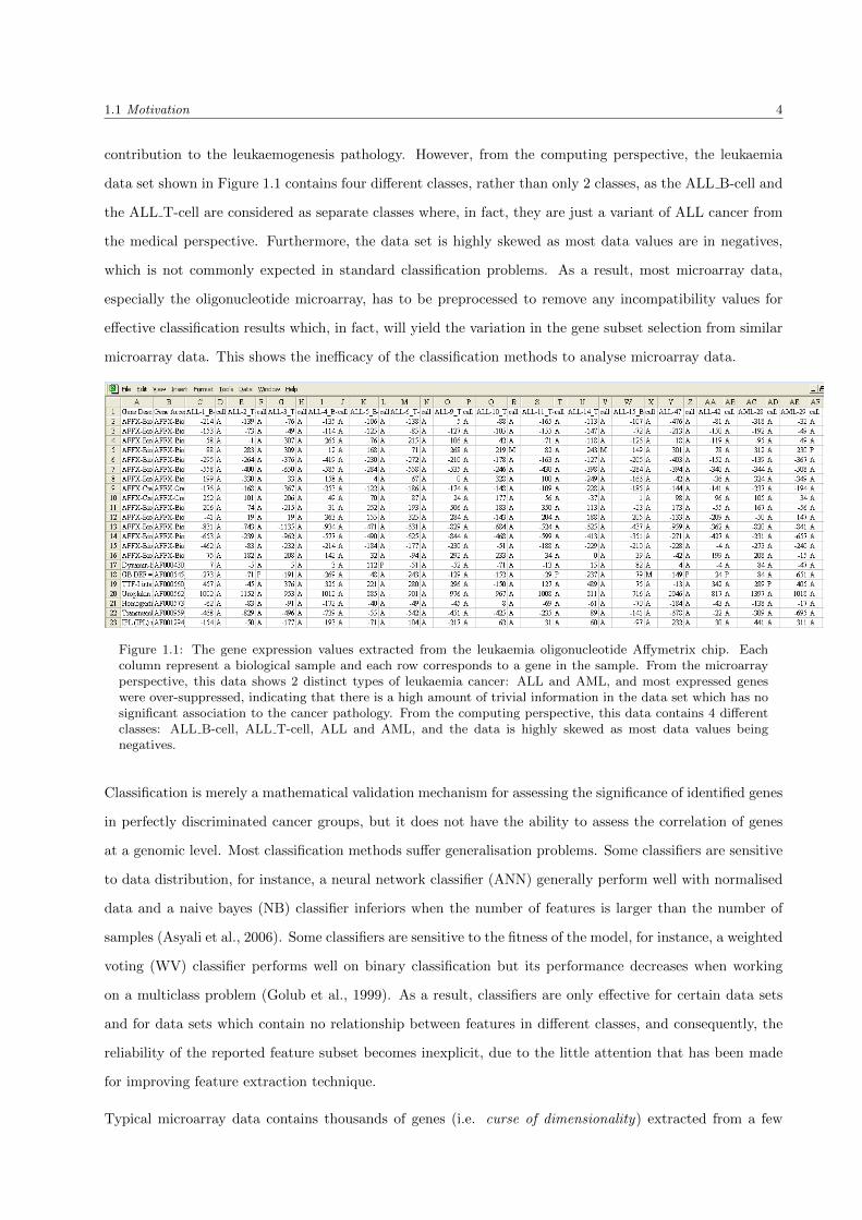
1.1 Motivation 4
contribution to the leukaemogenesis pathology. However, from the computing perspective, the leukaemia
data set shown in Figure 1.1 contains four different classes, rather than only 2 classes, as the ALL B-cell and
the ALL T-cell are considered as separate classes where, in fact, they are just a variant of ALL cancer from
the medical perspective. Furthermore, the data set is highly skewed as most data values are in negatives,
which is not commonly expected in standard classification problems. As a result, most microarray data,
especially the oligonucleotide microarray, has to be preprocessed to remove any incompatibility values for
effective classification results which, in fact, will yield the variation in the gene subset selection from similar
microarray data. This shows the inefficacy of the classification methods to analyse microarray data.
Figure 1.1: The gene expression values extracted from the leukaemia oligonucleotide Affymetrix chip. Eachcolumn represent a biological sample and each row corresponds to a gene in the sample. From the microarrayperspective, this data shows 2 distinct types of leukaemia cancer: ALL and AML, and most expressed geneswere over-suppressed, indicating that there is a high amount of trivial information in the data set which has nosignificant association to the cancer pathology. From the computing perspective, this data contains 4 differentclasses: ALL B-cell, ALL T-cell, ALL and AML, and the data is highly skewed as most data values beingnegatives.
Classification is merely a mathematical validation mechanism for assessing the significance of identified genes
in perfectly discriminated cancer groups, but it does not have the ability to assess the correlation of genes
at a genomic level. Most classification methods suffer generalisation problems. Some classifiers are sensitive
to data distribution, for instance, a neural network classifier (ANN) generally perform well with normalised
data and a naive bayes (NB) classifier inferiors when the number of features is larger than the number of
samples (Asyali et al., 2006). Some classifiers are sensitive to the fitness of the model, for instance, a weighted
voting (WV) classifier performs well on binary classification but its performance decreases when working
on a multiclass problem (Golub et al., 1999). As a result, classifiers are only effective for certain data sets
and for data sets which contain no relationship between features in different classes, and consequently, the
reliability of the reported feature subset becomes inexplicit, due to the little attention that has been made
for improving feature extraction technique.
Typical microarray data contains thousands of genes (i.e. curse of dimensionality) extracted from a few

1.1 Motivation 5
samples (i.e. curse of data sparsity) which are possibly obtained from the same arrays (source) because of
the high processing cost of microarrays, and, most of the genes in the microarray data are inter-related, as
shown in Figure 1.2. This complicates the process of finding informative genes. Numerous feature selection
techniques have been developed to extract informative genes, however, the core of the study is focused on
effective classification. For instance, Golub et al. (1999) introduced a signal-to-noise (S2N) ratio to improve
the classification performance of WV classifier in discriminating two dominant groups of acute leukaemia;
Khan et al. (2001) used gene signatures, identified by principal component analysis (PCA), to classify four
types of SRBCTs tumours using ANN classifiers and Tibshirani et al. (2002) developed a nearest shrunken
centroid (NSC) algorithm with respect to the prediction analysis of microarray (PAM) classifier. Albeit,
encouraging results had been achieved in most hybrid selection/classification models, the functionality of
the reported genes is inconclusive due to an ill-conceived hypothesis based on classification performance.
For instance, the S2N ratio calculates the correlation between individual genes based on the mean and the
standard deviation of the gene for the samples. This is not feasible for gene expression data as it omits the
correlation between a combination of genes. For instance, the ALL class in the leukaemia microarray data in
Figure 1.1 showed that there is more than one variant of ALL leukaemias, i.e. B-cell ALL and T-cell ALL.
Although, they are formed by different leukaemia cells, however, they shared some commonality in certain
genetic behaviour, i.e. lymphoblastic-based, which could be used as the signature markers in diffentiating
ALL patients from non-ALL cancer patients. Figure 1.2 shows the correlation between some expressed genes
in the leukaemia data which is presented in Figure 1.1.
Figure 1.2: The heatmap of the leukaemia microarray data. Each column represent a biological sample and eachrow corresponds to a gene in the sample. The density of the significant genes to the sample is presented withthe shade of two colours: red and blue. Shades of red indicate elevated expression (i.e. highly significant to thesample) while shades of blue indicate decreased expression (i.e. zero significant to the sample).
Furthermore, the implementation of more than one feature selection for the classification method may lead

1.1 Motivation 6
to different gene selection results due to over-complication in the model structure which could resulted in
model over-fit.
Over-fitting/under-fitting is a potentially serious problem in most computing algorithms, especially in the
classification methods. It occurs when the algorithm is learned for too long or too little. Normally, this
problem can be alleviated by continually monitoring the quality of training using a separate set of data.
However, there is no standard validation mechanism for assessing the algorithm’s performance. Some studies
validate the algorithm using a separate set of test data (Golub et al., 1999; Deutsch, 2001; Li et al., 2001a;
Hwang et al., 2002; Cho and Won, 2003; Liu et al., 2005b; Cho and Won, 2007; Zhang et al., 2008). Some
employed k-fold cross-validation procedures (Tibshirani et al., 2002; Cho et al., 2003b; Guan and Zhao,
2005; Osareh and Shadgar, 2008) to assess the performance of the algorithm. Some utilised leave-one-out
cross-validation procedures (Bø and Jonassen, 2002; Peng et al., 2003; Zhou and Mao, 2005; Zhou et al.,
2005; Chen et al., 2007) in the performance assessment. The over-fitting/under-fitting problem can also arise
when the algorithm has too many or too few parameters to learn, and consequently, its generalisation ability
may be inferior (Asyali et al., 2006).
The performance of a computing algorithm is usually defined based on a standard hypothesis that works
effectively in most real-world problems. This hypothesis is based on classification performance, i.e. ‘the
higher the classification accuracy obtained by the classifier, the better the solution to the problem’. However,
this hypothesis is not always correct in interpreting the gene correlation on microarray studies. Unlike
ordinary real-world data which has small levels of interaction between features, such as financial data,
bioassay data, intrusion data; microarrays has high complexity, as is depicted in Figures 1.1 and 1.2. The
genes in microarray data sets are all correlated either in a direct manner, for example, a high regulated
gene activates another gene with high expression, or in an indirect manner, for example, expression of a
gene is triggered by the detection of another genes. The p53 protein will only be activated by the presence
of the p53 gene (either highly expressed or has been detected) that contributes to the transformation and
malignancy of cells due to the failure to bind the consensus DNA binding site. The p53 protein is used to
co-ordinate the repair process of cells or induce cell suicide to stop any further growth of cancer cells. These
correlated genes may not be detected in high classification accuracy if the high individual correlated genes
are not presented or are “buried” by other more highly expressed genes.
There is an omission in the work of finding genes expressed in lower precision level, or, does not mention it at
all, due to the ill-conceived hypothesis and implicit research objective that was biased effective classification.
These genes, to some extent, may be important for early malignancy detection as some genes will only
become significant with the presence of its correlated genes which could be detected in lower precision levels.
The possible reasons for the immaturity of the computational analysis of microarrays is due to little un-

1.2 Statement of the Problem 7
derstanding of the complex relationship between genes and the importance of gene integration within a cell
or a tissue. As a result, the general hypothesis that worked effectively in ordinary real-world problems is
assumed to be effective for microarray data.
To conclude, our research is motivated by such challenges poses to the use of computational analysis on
gene expression aspects exposing several weaknesses, such as the implicit research objective and the ill-
conceived hypothesis, the normalisation of microarray data, the over-fitting problem and the omission of
genes expressed in lower precision levels.
1.2 Statement of the Problem
As mentioned in the previous section, research in microarray gene extraction is still inconclusive. Thus,
several problems on identifying informative genes have been exposed. This thesis concentrates on four main
aspects which are as follows:
1.2.1 Implicit Research Objective and Ill-conceived Hypothesis
Most research emphasises the effective classification and overlooks feature extraction. The analysis models
that were constructed based on the hypothesis emphasising the classification ability, which have been shown
to be successful in improving classification performance, but suffers from the problems of model fitness
and data distribution, as described in previous section. For instance, a conventional discriminant analysis
model requires more sample patterns than features (Culhane et al., 2002) to deliver high classification
results. Conversely, microarray data sets contain only a few sample patterns that are associated with
thousands of genes. Thus, the use of data preprocessing techniques and appropriate feature selection methods
to circumvent the problem are common solutions. However, such gene selections might involve arbitrary
selection criterion and overlook highly informative combinations of genes (Culhane et al., 2002). This is
due to microarray data containing more than one variant of cancer groups within a known cancer class, as
is shown in Figure 1.1 and a high correlation between genes expressed to a specific cancer disease, as is
indicated in Figure 1.2. Using the data preprocessing techniques, such as data normalisation, filtering and
data imputation, a potential consequence is that the features may end up equalised and what was originally
a primary feature may become of equal significance as secondary and less significant features. Furthermore,
the primary features may be removed in the filtering process and the features interactions may be altered
by improper impute values into some features. Thus, the lack of understanding of microarray data could,
possibly, lead to the improper research objectives outlined.

1.2 Statement of the Problem 8
1.2.2 Data Normalisation
There is often a large difference between the maximum and the minimum values within a gene in microarray
data, especially in oligonucleotide arrays, as is indicated in Figure 1.1. Some may be due to outliers, i.e.
values that are greatly different from the other values in the same gene, or missing values in the data. Thus,
data normalisation is usually expected to remove undesirable characteristics in microarray data to ensure
data integrity and better classification performance (Dudoit et al., 2002; Asyali et al., 2006; Kotsiantis et al.,
2006) rather than discovering correlated features. Normalisation, in the context of this thesis, is a scaling
process that reduces the magnitude of data values to a specific range and the degree of scaling is reliant on
the mathematical formulas applied. Data normalisation is normally expected in a classification problem, as
it is a very effective way of removing unwanted features from the data set, in particular when the features
are not correlated. In microarray data, due to the complex biological interaction between expressed genes,
normalisation is not always versatile. Conversely, it may deteriorate the finding of the correlated genes, in
response to the labelled classes, by compressing the intensity of expressed genes to minimal. As a result,
the correlated genes expressed in a lower expression level may be ignored. Furthermore, different types of
normalisation technique may also produce different set of data values on the similar data set. Table 1.1
shows some examples of the relevant work on the leukaemia microarray data involving data preprocessing
as shown in Figure 1.1.
Table 1.1: Some examples of the work related to the leukaemia microarray data.
Author Data preprocessing Selection method Classification method
Golub et al. (1999) Mean and deviation nor-malisation
S2N ratio WV
Culhane et al. (2002) for COA: negative valuestransformation; for PCA:mean and deviation nor-malisation
COA, PCA BGA
Dudoit et al. (2002) thresholding, filtering,log-transformation, meanand variance normalisa-tion
BSS/WSS ratio various discriminationmethods
Li and Yang (2002) Log transformation Stepwise selection LRM
Lee and Lee (2003) as similar to Dudoit et al.(2002)
BSS/WSS ratio SVMs
Mao et al. (2005) as similar to Dudoit et al.(2002)
RFE SVMs
Cho and Won (2007) Max-min normalisation Pearson correlation ensemble ANNs

1.2 Statement of the Problem 9
Dudoit et al. (2002); Mao et al. (2005) and Lee and Lee (2003) conducted a comprehensive preprocessing step
comprising values truncation, genes ratio filtering and log (base-10) transformation on the data set before it
has been standardised using zero mean and unit variance. Consequently, the integrity of the gene selection
results have been compromised by these over-compressed techniques. Golub et al. (1999), on the other
hand, standardised the similar data set using different mathematical formula. Instead of using the variance
parameter (i.e. the square of the standard deviation), Golub et al. used standard deviation function. Cho
and Won (2007) adopted maximum-minimum function to scale down the magnitude of the data set into the
interval [0,1]. Li and Yang (2002), however, used only the log transformation to scale down the data values
in the data set. Culhane et al. (2002) converted all the negative expression values in the data set to positive
values before performing normalisation technique. This has, in fact, altered the context of the expression
values in the genes, i.e. from the original inhibitory became excitatory.
1.2.3 Over-fitting Problem
Over-fitting normally arises when the algorithm has learned too much due to several factors, such as an
over-parameterised model structure, too many repetition assessments in the algorithm and the complexion
of the algorithm. A typical example is the use of an external feature reduction method to filter the redundant
features and then analyse the remaining features with different selection approaches that are embedded in
the classification technique. As shown in Table 1.1, Dudoit et al. (2002); Mao et al. (2005) and Lee and Lee
(2003) used a normalised matrix of intensity values to filter the least significant genes of the leukaemia data
set before the selection method was applied. As a result, the correlated genes may have been discarded in
the filtering process and over-optimistic classification results were reported.
1.2.4 Omission on Features expressed in Lower Precision Level
In existing bioinformatics literature, the reported gene selection results are based on the optimum classifi-
cation accuracy. Thus, the correlated genes expressed in the lower accuracy have not received any attention
as these genes do not possess a predictive benefit in a classification result. This may lead to disregarding
the ‘true’ underlying genes responsible for the early stage of a cell abnormality. A possible approach to
solving this problem is to monitor differentiation of the genes expressed in different precision levels. The
main advantage of this approach is to provide a concrete formulation on the reported genes.
The outline of our approach to solve these problems is presented in the next section.

1.3 GANN: Feature Extraction Approach 10
1.3 GANN: Feature Extraction Approach
This thesis focuses on extracting informative features from the data set that contains high feature dimension
and feature correlation, as well as sample scarcity.
According to existing bioinformatics literature, none of the computational classification models are superior
to the other. This is due to the implicit research objective and model abilities in extracting informative genes.
Although many variants of hybrid selection/classification methods have been proposed, the performance of
the models are still heavily reliant on the characteristics of the data sets and the nature of classification
methods. In our solution, we analyse differentially expressed microarray genes using genetic algorithms
(GAs) and artificial neural networks (ANNs).
The reasons for choosing GA and ANN in this research are that they are the only two algorithms based
on the analogy of nature and have received high recognition for the delivery of promising results from
various disciplinary areas, such as medical diagnosis (Dybowski et al., 1996; Khan et al., 2001; Djavan et al.,
2002; Zhang et al., 2005; Froese et al., 2006; Heckerling et al., 2007), environmental forecasting (Nunnari,
2004; Fatemi, 2006; Nasseri et al., 2008), hardware utilisation prediction (Barletta et al., 2007; Taheri and
Mohebbi, 2008), real-time series prediction (Kim and Han, 2000; Sexton and Gupta, 2000; Arifovic and
Gencay, 2001), food lifespan forecasting (Gonia et al., 2008), sonar image reading (Montana and Davis,
1989) and computational problem (Sexton and Dorsey, 2000; Kwon and Moon, 2005; Cheng and Ko, 2006;
Hu et al., 2007). The ANN is a universal computation algorithm that has the ability to compose complex
hypotheses that can explain a high degree of correlation between features without any prior information
from the data set (Cartwright, 2008a). Meanwhile, the GA is an effective population-based search algorithm
designed for a large, complex and poorly understood data space due to its ability to exploit accumulating
information about this unknown data space and to bias subsequent a search into useful subspaces (DeJong,
1988). In addition, GA is robust from trapping into local minima, i.e. the over-fitting problem (Montana
and Davis, 1989).
GA/ANN hybrid systems are not new in microarray classification, but, are innovative for gene extraction.
Several examples of GA/ANN hybrid systems on classification include breast metastasis recurrence (Bevilac-
qua et al., 2006a,b), multiclass tumour classification (Cho et al., 2003a; Karzynski et al., 2003; Lin et al.,
2006) and DNA sequence motif discovery (Beiko and Charlebois, 2005). In these studies, the data sets were
normally normalised and partitioned into several smaller sets to ensure better classification performance of
the system. The GA acts as a supporting tool to optimise the classification performance of ANN. This could
contribute to the gene variability in the selection results. Rather than emphasize classification performance,
our research focuses on the extraction ability of the hybrid GA/ANN. Our approach optimises the connection

1.3 GANN: Feature Extraction Approach 11
weights of ANN and, at the same time, evaluates the fitness function of the GA using 3-layered ANNs. The
distinct difference between the existing GA/ANN hybrid systems and our GA/ANN hybrid approach is that
rather than using ANN as a classifier to predict cancer classes, the ANN in our approach is act as a fitness
score generator to compute the GA fitness function. Figure 1.3 presents the graphical hybridisation of the
GA/ANN approach used for classification and our selection approach.
(a) A typical GA/ANN hybrid system for microarrayclassification.
(b) The proposed GANN hybrid system formicroarray gene extraction.
Figure 1.3: A typical GA/ANN hybrid classification model and the proposed GANN feature extraction model.The diagram (a) shows a typical GA/ANN hybrid system used in microarray classification. In this hybridsystem, the ANN is used as a classifier to discriminate between cancer classes. The diagram (b) presents theproposed hybrid system focusing on the extraction of informative genes from microarray data. In our system,the ANN is act as a fitness score generator to compute fitness score for GA.
Fitness function is the most crucial aspect in GA as it determines the effectiveness performance of GA.
Most research concentrates on optimising other aspects of GA and only a few studies on improving GA
fitness function, e.g. the use of a penalty function to identify invalid chromosomes and approximating fitness
evaluation within a given amount of computation time (Beasley et al., 1993). However, these approaches
require an additional task level in a GA algorithm, for instance, a set of rules for determining the invalidity
of chromosomes, i.e. how poor the chromosome is, and a set of mathematical formulas to compute penalty
values when GA selecting invalid chromosomes, and consequently, the optimisability performance of GA

1.4 Research Question and Hypotheses 12
relies heavily on how ‘good’ this additional function is in finding the ‘optimal’ fitness function. Some
studies proposed the use of effective classifiers on fitness computation, for instance, Li et al. (2001b) used
the classification result returned by k-nearest neighbour (KNN) as the fitness function of GA on acute
leukaemia classification, Cho et al. (2003a) computed fitness function based on neural network prediction
results on SRBCTs tumours, Lin et al. (2006) and Bevilacqua et al. (2006b) employed error rate returned
by neural network classification as GA fitness function on multiclass microarray data and breast cancer
metastasis recurrence, respectively. In our approach, instead of letting the user determine the level of invalid
chromosomes, we use simple feedforward ANN to compute fitness values for GA chromosomes. A novel
feature of our approach is based on the explicit design of the algorithm which explores the potentialities of
the GA and ANN methods of extracting informative features with minimal structural requirements on GAs
and ANNs, as followed the Ockham’s Razor principle.
Figure 1.3b shows our hybrid approach. To formulate an effective feature extraction method and to circum-
vent the over-fitting problem, a GA is used to initialise a population of chromosomes in which its fitness
value is computed using a 3-layered feedforward ANN with centroid vector principle and Euclidean distance.
Once all chromosomes are assigned with fitness values, a set of genetic mechanism is used to assess the fitness
of the chromosome and the least fit chromosome is replaced by a new chromosome. Through evolution over
many generations, ANN connection weights and GA fitness function are optimised, the least fit chromosomes
are gradually replaced by new chromosomes produced in each generation and the optimal set of genes are
obtained.
1.4 Research Question and Hypotheses
The research questions are derived from the problems identified in existing literature. Thus, two of our
research questions are as follow:
1. Can we use the simplest parameters in both GA and ANN to solve the problems stated in Section 1.2?
The simplicity in this context referring to the use of the minimal necessity parameters in both GA and
ANN to extract optimal gene subset from the raw (i.e. unprocessed) microarray data.
2. Can we identify informative genes which underly different precision levels in the microarray data?
The precision level in this context referring to the minimum fitness accuracy required by the model in
selecting informative genes from the raw, unprocessed microarray data.
These questions yield the aim of this research which is to devise a more effective way for extracting informative
features using machine learning methods. Thus, the hypotheses focuses on the outcomes of the research and

1.5 Contributions 13
on the conceptual design of hybridising GA and ANN methods. A feature extraction system has been built
based on these hybridised techniques. The hypotheses are as follow:
1. Without the use of acceleration techniques in ANN, the feedforward learning is able to compute the
GA fitness function (Model simplicity, generalisability and normalisation-free).
2. The proposed technique is able to detect genes that are differentially expressed in different tumour
development stages, i.e. different fitness precision levels (Biological plausible results).
These hypotheses are tested by the design developed in Chapter 3, the prototype and the experimental study
in Chapter 4, and the experimental results and discussion in Chapter 5.
1.5 Contributions
The aim of this research is to formulate, from the identified computing-related problems stated in Section
1.2, an innovative feature extraction model using machine learning methods for extracting informative and
relevant features using GAs and ANNs. This aim leads to major contributions, which are as follow:
• The realisation of problems pertaining to microarray experiment and the data structure of microarrays.
Unlike ordinary real-world data which has small level of interaction between features and high sample
size, microarray data contains thousands of genes associated with less than a hundred samples that
have been collected from various sources, which could, possibly, yield heterogeneity solutions in gene
combinations to the data. Additionally, genes in the microarray data are all correlated to some extent.
The aim of microarrays is to provide biological insights into gene interactions for the design of a
treatment strategy at the molecular level, instead of finding genes that can perfectly discriminating
between cancer classes. This realisation leads to the inducement to design a novel feature extraction
approach with as minimal an involvement of statistics as possible.
• A practical approach to identifying informative genes using an innovative hybridising GA and ANN.
This solution will assist in answering the problems addressed in Section 1.2.
• A prototype to realise the proposed techniques. This prototype will assist in validating the hypotheses
and in providing the fundamental basis for conducting an experimental study.
• The analysis of experimental results to indicate the cognitive performance of the prototype in different
precision states and the effect of an innovative hybridisation solution, as well as to demonstrate the
significance of the identified genes from a biological perspective.
• The publications of experimental result to various conferences.

1.6 Structure of Thesis 14
In additional to major contributions, the minor contributions stemming from this thesis are as follow:
• The review of existing bioinformatics literature pertaining to cancer classification and gene selection
techniques. The strengths and limitations for classification techniques, feature selection and/or reduc-
tion techniques and model evaluation approaches were discussed to determine the unresolved problems.
• The identification of informative genes in different stages of tumour development may enhance the
insight of the gene-gene interaction in the growth of abnormal cells and may assist practitioners in
designing treatment strategies to prevent further progression of a cell abnormality.
• The research in optimising GA fitness function. In our approach, the fundamental ANN paradigm
is exploited to increase the capability of the existing fitness optimisation techniques on the aspect of
improving the performance of GA.
1.6 Structure of Thesis
This thesis contains six chapters and three appendices. Chapter 2 explores the literature of the human
microarray cancer analysis framework. The literature covers the current works in the field and details the
intrinsic evaluation between existing works. The current works such as techniques for creating microarrays,
selection approaches for the selection of highly expressed genes in the cancer classes, classification methods
for discriminating sample patterns and validation mechanisms for validating the performance of classification
methods are reviewed.
Chapter 3 describes the planning and design phases that have been carried out to deliver the theme of this
research. A conceptual design of our feature extraction prototype namely, Genetic Algorithm-Neural Network
(GANN), is designed to study the interaction between informative genes that trigger the proliferation of a
specific tumour disease. In this chapter, the experimental data sets, used in supporting our research theme
will be discussed. These data sets including two synthetic data sets, two benchmark microarray data sets,
i.e. ALL/AML and SRBCTs, and two bioassay data sets, i.e. AID362 and AID688. The accuracy (i.e.
correctness) of the selection results will be evaluated with synthetic data sets and the robustness of the our
model in dealing with large data sets will be examined with bioassay data sets.
Chapters 4 and 5 describe the prototype and experiments of our approach to identify informative genes
that underlies the data. Chapter 4 describes software tools and the experimental study used to support
this thesis, including the prototype of our model, and Chapter 5 evaluates the reliability of our approach by
comparative studies of our results with four commonly used ANN activation functions, i.e. sigmoid, linear,
hyperbolic tangent (tanh) and threshold, as well as the results from the original studies. The insight of the

1.6 Structure of Thesis 15
identified genes will be verified against NCBI genbank via the Entrez Gene search system and the Stanford
SOURCE search and retrieval system.
Chapter 6 concludes our work and direction for future work. Our method will be evaluated based on the
goal achievement and further improvement in the method will be discussed. Finally, the thesis is concluded.
Chapter 2
Background and Literature Review
Chapter 1 gave the overview of our solution to the problems concerning informative genes detection in Section
1.2. This chapter describes the literature related to the problems and solution presented in this thesis, from
both the biological and the computing perspectives.
This thesis describes an intelligent gene extraction method using hybrid GAs and ANNs in microarray studies.
Hence the related literature from a biological perspective includes microarray production and its challenges,
and the computing perspective includes data preprocessing, classification and prediction modelling, as well
as computational challenges.
This chapter contains three sections. Section 2.1 provides the background on microarrays. Aspects concern-
ing the array design, fabrication techniques, fluorescent labelling systems and microarray-related problems
will be presented. Section 2.2 reviews computing approaches that have been used in cancer microarray
analysis, including data preprocessing approaches, classification and prediction techniques, model validation
mechanisms and aspects pertaining to the problems set out in Section 1.2. Section 2.3 provides a summary
of the chapter and to what follows next in the thesis.
2.1 A Biological Perspective
The understanding of genetics has advanced remarkably in the last three decades since the first recombinant
DNA molecule in the early 1970s. DNA plays a vital role in our daily activity as it makes cells more
specialised to perform certain functions, for example pancreatic cells to produce enzymes and insulin for
digesting food, or red blood cells to produce haemoglobin to transport oxygen to other cells (oxygenated)
and to carry carbon dioxide/monoxide away from cells. To do so, DNA makes ribonucleic acid (RNA) by
unbinding DNA strands to synthesise message RNA (mRNA). The mRNA is then sythesises with amino
16

2.1 A Biological Perspective 17
acid units to produce proteins to make cells function. Pragmatic studies have been performed to find a way
to measure DNA gene expressions in order to study the cancer biology of some genetic diseases over the last
decade and this has led to the vast development of publicly available repositories for microarray experiments
and microarray data. Table 2.1 presents examples on well-recognised resources for microarray experiments
and repositories. A microarray is the DNA chip that is used to store and to analyse the information contained
within a genome (the entire DNA sequence of a particular organism) or proteome (the entire complement of
proteins expressed by a genome). A microarray contains microscopic spots, i.e. the identical single-stranded
deoxyribonucleic acid (DNA) that attach to a solid surface, which is then used to detect the presence and
abundance of labelled nucleic acids in a biological sample. In the process of making microarrays, messenger
RNA (mRNA), transfer RNA (tRNA) or complementary DNA (cDNA) are extracted from the sample RNA
and labelled with a fluorescent dye system, these DNA probes are then hybridised and scanned to produce
an image of the surface of the array (Ebert and Golub, 2004). Figure 2.1 on page 19 presents the making of
microarrays based on two widely used DNA probes, i.e. cDNA and oligonucleotide arrays.
The microarrays quality and interpretation are influenced by the type of probe used, the way in which the
probes are aligned onto a solid support and the technique of target preparation (Ebert and Golub, 2004),
thus, great care is taken in conducting microarray experiments. In all cases, the first step is to extract the
RNA from the tissue/cell of interest by diluting the biological sample with certain chemical substances and
the RNA is then amplified using polymerase chain reaction (PCR) assays. The subsequent sections describe
the steps in the microarray experiment, including array design, fabrication technologies, labelling systems,
hybridisation and image analysis. This section concludes with problems concerning the cDNA arrays.
2.1.1 Array Design
At present, two prevalent approaches for DNA arrays are cDNA and oligonucleotide arrays, depicted in Figure
2.1, adopt different experimental platforms. The clone-based platform is used to produce cDNA arrays, while
the oligonucleotide-based platform is used to create a high density of oligonucleotide arrays. Both arrays
exploit hybridisation, however, they differ in terms of probe lengths and its composition, layout of sequences
in the array, cross-hybridisation and hybridisation effects from an immobilised substrate (Mah et al., 2004),
as well as objectives of the studies. For the studies where the focus is on a specific subject area and the
abundance ratio of differentially expressed genes is needed, such as genes relevant to particular metabolic
pathways, the low-density of cDNA array is required. Whereas, for the studies where little prior information
on relevant genes is available, or where an unbiased overview of global changes in gene expression patterns
is required, the high-density of oligonucleotide array is the best option (Tomiuk and Hofmann, 2001). Table
2.2 on page 21 presents a comparison study based on cDNA and oligonucleotide arrays, along with their

2.1 A Biological Perspective 18
Table 2.1: Resources for microarray experiments and microarray repositories.
Website URL Resources
National Center for Biotechnol-ogy Information (NCBI)
http://www.ncbi.nlm.nih.gov/ GEO database, genbank,analysis software, searchbrowsers
European Bioinformatics Insti-tute (EBI)
http://www.ebi.ac.uk/arrayexpress genbank, biological on-tology, ArrayExpressdatabase
National Human Genome Re-search Institute (NHGRI)
http://research.nhgri.nih.gov/ cDNA microarray proto-cols, cDNA microarrayrepository, analysis soft-ware
Broad Institute, cancer genomicgroup
http://www.broad.mit.edu/ analysis software, mi-croarray repository &associated articles
Standford University, genomicdepartment
http://smd.stanford.edu/ experiment protocols,SOURCE & AmiGObrowsers, analysis soft-ware, cDNA microarrayrepository
Microarray Gene ExpressionData (MGED) Society
http://www.mged.org/ MIAME standard, geneontologies, MAGE
GO Consortium http://www.geneontology.org/ gene ontology and partici-pating laboratories
distinct advantages and disadvantages.
cDNA arrays containing cDNA fragments that are generated by PCR amplification of the cDNA clone, which
is the reverse-transcriptase of two different biological samples mRNA that are labelled with different dye
colours and hybridised to DNA sequences, that are robotically spotted on the surface of the glass slide (Ebert
and Golub, 2004). After hybridisation, a special scanner is used to measure the intensity of fluorescence of
each differentially expressed gene on a fine grid of pixels and to produce the digital image of hybridised arrays.
Normally, higher fluorescence indicates a higher expression value of the gene in the sample. The cDNA array
is relatively simple to produce and is inexpensive for laboratories with access to robotic equipment, however,
it needs careful attention to the chemistry which adheres the DNA to the glass (Ebert and Golub, 2004).
A lack of standard procedure due to manufacturing errors and improvised techniques used in producing
high-quality cDNA arrays by individual research laboratories has caused more unnecessary problems than
one might expect. For instance, the primary technical difficulty in microarray experiments is the amount
of each DNA probe that is robotically spotted on different arrays. To control inconsistency, sample RNA
is often hybridised with a defined amount of reference RNA that is labelled with a different fluorescent

2.1 A Biological Perspective 19
Figure 2.1: The microarray experiments: Oligonucleotide versus cDNA arrays. In all microarray experiments,the RNA is extracted from the biological sample and the RNA is then amplified using PCR assays. For oligonu-cleotide microarrays, the probes are directly synthesised onto solid surface and the single-dye colour is used toread the gene expression in the sample. For cDNA microarrays, the PCR products from cDNA libraries aredeposited onto a solid surface and the two-dye colour is used to read the gene expression in the samples.
dye (Ebert and Golub, 2004). However, this yielded another technical concern, that is, the amount of
reference RNA in the hybridisation process is dependent on the amount of probes that are robotically spotted
and also the manufacturer’s guideline. Additionally, cDNA probes often contain repetitive sequences, as a
result, the process becomes intensive, especially when the experiment is conducted on a genome-wide scale,
consequently, the cross-hybridisation has become more problematic (Ebert and Golub, 2004). A significant
advantage of cDNA array is that it does not require prior sequence information due to it being initially
designed for sequence modelling. Thus, it is an attractive alternative for model organisms whose genomes
are not yet sequenced (Ebert and Golub, 2004). The disadvantages of cDNA array are, inconsistency in
the procedure adopted by the individual research laboratories and manufacturers resulting in a variation in
gene measurements, intensive computational cost on a genome-wide scale experiment and is problematic on
cross-hybridisation due to repetitive sequences in cDNA microarrays.
Comparing to cDNA arrays, high-density oligonucleotide array is an active area of technological development
(Parmigiani et al., 2003) and the most widely used oligonucleotide arrays are manufactured by Affymetrix
(Santa Clara, CA) which uses the in-situ photolithographic synthesis technique to produce oligonucleotides

2.1 A Biological Perspective 20
onto the array chips. Therefore, oligonucleotide arrays, also referred to as Affymetrix arrays, are less prob-
lematic than cDNA arrays. The oligonucleotide arrays contain short oligonucleotide probes with a length
between 25 and 60 mers (base-pairs) that are either synthesised in-situ or robotically spotted on the surface
of the glass side. In oligonucleotide array, sample RNA is prepared, labelled with dye colour and hybridised
to an array which is then scanned into digital image to obtain a fluorescence intensity value for each probe.
Unlike cDNA arrays, oligonucleotide arrays use single-channel labelling system, i.e. single dye colour, in
hybridisation and each oligo probe contains a unique oligonucleotide sequence (Ebert and Golub, 2004) that
ease the hybridisation process. Due to the short probe length in oligonucleotide arrays, the hybridisation
specificity is more easily controlled than cDNA arrays.
Literature (Mah et al., 2004; Asyali et al., 2006) shows that although cDNA and oligonucleotide arrays have a
poor correlation on the DNA probes, both arrays are able to display similar characteristics in the data, even
though, the combined results of both arrays have been not possible. Hence, studies on the combination of
results on multiple similar arrays have gained close attention from the bioinformatics field. With the robust
and reproducible gene expression data that can be generated on multiple similar arrays, the technicality
aspects of array design have become less critical (Ebert and Golub, 2004). However, the degree of similarity
of the DNA probe sets and the expression level of the corresponding transcript in the experiments still play
important roles in the reproducibility aspect and yet, this issue remains a topic of intensive research (Asyali
et al., 2006).
2.1.2 Fabrication Technology
Two prevalent microarray fabrication technologies in microarray experiments are robotic spotting and in-
situ synthesis. The robotic spotting synthesises DNA probes prior to the array deposition which is then
detected onto glass, while the in-situ synthesis synthesises DNA probes directly onto the array surface
without depositing intact DNA probes.
For robotic spotting, robotic-controlled pins are dipped into wells that contain DNA probes and then deposited
each probe at the designated locations on the array surface. The amount of probes collected depend on the
number of arrays being made and the amount of liquid the pins can hold. The pins are then washed to remove
any residual solution before the next sample is collected to prevent contamination on the subsequent sample.
Once all locations on the array are occupied with probes, the known reference template, i.e. complementary
cDNA or cRNA “targets” derived from experimental samples which represent the nucleic acid profiles is
prepared to hybridise with cDNA probes. The probes spotted by the spotting technique can be cDNA,
oligonucleotides or even small fragments of PCR products that correspond to mRNA.
For in-situ synthesis, the probes are short oligonucleotide sequences, in the range of 25 to 60 mer probes, that

2.1 A Biological Perspective 21
Table 2.2: A comparison between cDNA and oligonucleotide arrays.
Description cDNA arrays Oligonucleotide arrays
Platform design clone-based Oligonucleotide-based / Affymetrix-based
Probe length Long sequence Short sequence, approx. 25 - 60 mer(base pair)
Fabrication tech-nique
Robotic spotting Synthesising in-situ
Labelling system Two-dye fluorescent colours Single-dye fluorescent colour
PCR correlation Low High
Production cost Low High
Normalisation Yes (pre- & post-normalisation) Yes (pre-normalisation)
Advantages Emphasize on genes related to a specificsubject areas
Unbiased overview on the global fluctu-ations in gene expression patterns
Easily customise Less sensitive to cross-hybrdisationNo prior information on cDNA se-quences required
Uniformity of probe length and the abil-ity to discern splice variantsAble to recover samples after hybridis-ation to a chip
Disadvantages Difficulties on the production of high-quality cDNA arrays
Sensitive to base pair changes due toshort length of DNA probes involved
Variability in gene expression measure-ment
Requires prior information on relevantgenes
Vulnerable to cross-hybridisationProblems on reproducibility of genesMay contain latent non-specific DNAsequences
are built up base-by-base on the array surface that are designed to match parts of the known sequence (Stekel,
2003a). With each added nucleotide to the array, there is a protective group to prevent more than one base
being added during each round of synthesis. This protective group is then converted to a hydroxyl group,
either with photolithographic synthesis or chemical reagents via inkjet technology. The photolithographic
synthesis approach uses light to convert the protection group, while the reagent approach employs a similar
chemistry substance as a standard DNA synthesiser and droplets of the appropriate base are fired at each
step of synthesis onto the desired spot via inkjet printers which fires adenine (A), cytosine (C), guanine (G)
and thymine (T) nucleotides. The main advantage of the inkjet approach over photolithographic synthesis
arrays and spotted arrays is that the gene synthesis process is highly flexible as it is fully controlled by
the computer, based on the user requirement. However, it is less efficient for making a large quantity of
identical arrays (Stekel, 2003a). Chemical reagents via inkjet technology have been used by some reputable
laboratories such as Rosetta, Agilent and Oxford Gene Technology (Tomiuk and Hofmann, 2001; Stekel,

2.1 A Biological Perspective 22
2003a).
At present, there are two types of photolithographic synthesis: masks and maskless. The masks photolitho-
graphic synthesis is the basis of the Affymetrix technology that uses masks to allow light to pass to a certain
area of the array and at each step of synthesis, different types of masks are required (Stekel, 2003a). The
maskless photolithographic synthesis used by Nimblegen and Febit, employs a computer-controlled mirror to
direct light to the desired parts of the glass slide at each step of synthesis (Stekel, 2003a).
2.1.3 Labelling Systems
After RNA is extracted and fabricated, the sample can then be labelled. The labelling process can be either
fluorescence or radioactive, depending on the fabrication technique used in the microarray experiment. This
thesis focuses on the fluorescence labelling system as it is the most commonly used system rather than the
radioactive system. Two types of fluorescence labelling systems for oligonucleotide and cDNA arrays are
single-channel (i.e. single-dye) and two-channel (i.e. two-dye) systems, respectively.
On Affymetrix arrays, i.e. oligonucleotide arrays, a biotin-labelled cRNA is constructed for hybridising to
the Affymetrix GeneChip, thus, a single-channel is commonly used to show the expression values of given
genes. A significant advantage of single-channel labelling is that the collected data can represent absolute
expression values of genes, as a result, an aberrant sample cannot affect the data collected from other samples
as each array chip can only hold one sample as opposed to a two-channel labelling system where an array
chip is exposed to many samples, i.e. cross-hybridisation. Consequently, the overall data precision on 2-
channel labelling system could be affected if there is an outlier between samples in the chip. Additional
strengths of the single-channel system are the comparison studies between arrays which can be conducted
in noncontinuous time frames, such as months or years and the combination results of multiple arrays on
different array chips are possible as a similar dye colour system is applied. A significant drawback of this
labelling system is that it requires more array chips to store the data.
Meanwhile, on cDNA arrays, cDNA probes and reference template are differentially labelled with two flu-
orophores to allow for the quantification of differential gene expression. Expression values are reported as
ratios between two fluorescent values (Ramaswamy and Golub, 2002), as shown in Figure 2.2. Two samples,
i.e. disease cell versus normal cell, are compared and labelled using two different fluorescent dyes, normally
with Cy3 corresponding to the green fluorescent probes and Cy5 corresponding to the red fluorescent probes.
These two Cy-labelled cDNA samples are then hybridised to a single microarray using control probes pro-
vided by oligonucleotide microarrays which is then scanned to visualise the fluorescence of the probes after
they have been excited with a laser beam. The fluorescence intensities of each probe are then normalised,
based on the preselected control probes and analysed using a specially designed computer algorithm to detect

2.1 A Biological Perspective 23
the regulation of genes. A two-channel system is prone to dye biases due to different dye properties and dye
ability which result in a variation in gene expression measurements using the same DNA sample (Parmigiani
et al., 2003). To remove dye biases, additional normalisation is performed after digitising hybridised arrays,
which is elaborated in Section 2.1.5.
Figure 2.2: A typical 2-channel microarrays. The RNA are extracted from the normal and disease cells andamplified using the PCR assays. The RNA are then reverse-transcriptase into the cDNA, which is then labelledwith two different fluorophores using two-channel labelling system. Two fluorescent dyes for cDNA labelling areCy3 (green) and Cy5 (red). The two Cy-labelled cDNA samples are mixed and hybridised to a single microarraythat is subsequently scanned in a microarray scanner to visualise the fluorescence of the fluorophores after theexcitation with a laser beam of a defined wavelength. The intensities of each flurophore are then be used in theratio-based analysis to identify the regulation of genes.
2.1.4 Hybridisation
After DNA probes have been labelled with a proper dye system, hybridisation is performed by complemen-
tarily combining DNA probes and the labelled RNA reference template. Hybridisation can be performed
either manually or robotically. In the past, the sample has been manually hybridised and, to date, due to the
advance of biology technology, most research laboratories use robotic hybridisation which can provide a much
better control of the temperature of the target and slide (Stekel, 2003a), thus reducing the variability error

2.1 A Biological Perspective 24
in gene expression measurement. In addition to the ambient condition factor, variability errors can also arise
from other factors, such as salt concentrations, formamide concentration, target solution volume and oper-
ator, edge effects (effects seen only at the gene spotted near the edges of the array) and cross-hybridisation
(Stekel, 2003a; Parmigiani et al., 2003).
2.1.5 Image Analysis
The final step of microarray experiment is to produce an image of the hybridised array. A special scanner
is used to read the fluorescent dyes on the surface of the glass slide that are excited by the scanner laser
beam. In order to make a digital image of the array, the laser must focus at the desired point on the array
so that the dye at that point is excited by the laser and then detected by a photo-multiplier tube (PMT)
in the scanner (Stekel, 2003a). The quality of the digital image is generally associated with fabrication
techniques, hybridisation and dye labelling. For instance, Affymetrix arrays have light refraction problem on
the masks photolithographic synthesis, thus, it is compensated by a high quality of image processing software
(Stekel, 2003a), meanwhile spotted array images can be of variable quality, depending on the variation in
hybridisation and differential dye labelling (Auburn et al., 2005).
After producing a digital image of the array, some form of normalisation is generally applied to microarrays to
remove any form of biases yielded by fluorescent dyes used to label cDNA-based samples (Leung and Cavalieri,
2003; Wilson et al., 2003). There are two major groups of normalisation, i.e. within-array and between-
array normalisation. The within-array normalisation compares samples of a single array chip, meanwhile the
between-array normalisation makes comparisons between samples hybridised to multiple array chips.
The within-array normalisation generally involves either fitting a regression line to the log intensities of
dyes versus average intensity of each probe (Stekel, 2003b) or to form a smooth curve (lowess curve) based
on the joining of a large number of local regressions in every subset of data using log intensities of dyes
(Leung and Cavalieri, 2003; Stekel, 2003b; Wilson et al., 2003). However, a significant drawback of within-
array normalisation is that it is based on the assumption that a majority of the genes are not differentially
expressed (Stekel, 2003b).
The between-array normalisation, on the other hand, involves the global normalising gene expression based
on the equalisation of expression using the mean of all genes within an array across the mean of all expressed
genes from different arrays (Asyali et al., 2006; Leung and Cavalieri, 2003), with a core assumption that
genes can be differentially expressed as a result of the experimental condition and do not represent biological
variability (Stekel, 2003b; Asyali et al., 2006). However, depending on the biological conditions of different
arrays, this assumption could be violated. A solution to this violation is to use a set of common housekeeping
genes on the arrays to replace the mean expression normalisation of all the genes in the array or the known

2.1 A Biological Perspective 25
amount of exogenous control genes to be added to the finished microarrays. Housekeeping genes are genes
that have stable differential expression across different biological conditions (Asyali et al., 2006) with a low
differential expression and a small variability after normalisation (Wilson et al., 2003). Recent reviews show
that housekeeping genes are not as constantly expressed as was previously assumed (Leung and Cavalieri,
2003) and improper use of housekeeping genes may yield another potential source of error. Hence, the use
of the dye-swapping experiment is seen as a plausible solution. However, this experiment is impractical in
use, due to the limited supply of samples that fulfil certain criteria (Leung and Cavalieri, 2003).
To conclude, fluorescence biases are primarily dependent on the average expression level and spatial position
of the probe in the cDNA microarrays in which such conditions are determined by several factors, including
the experimental protocols, the lengths of probes, the number of tissues to be measured per array and the
array size (see Section 2.1.1). Therefore, the post-normalisation in the image analysis phase (see Section
2.1.5) is used to remove biases yielded from such conditions, but not to remove biases caused by other factors
such as printing resolution, scanning efficiency, labelling efficiency and PCR assays.
2.1.6 Microarray Challenge
cDNA microarray has been widely studied over the last decade, however, it is still imperfect in some ways
due to some technical problems incurred during the production process. The key problem is the variability
in gene expression measurements using the same DNA sample. This variability arises in almost every phase
of the cDNA microarray experiment, such as sample preparation (amplification, purification, concentration,
spotting volume), sample labelling (dye properties), hybridisation (ambient conditions, spotting effects,
cross-hybridisation) and image processing (scanner property, image algorithm and settings) (Parmigiani
et al., 2003). Although these errors are relatively small, however, the compounding of their effects can be
severe, particularly, in verifying the underlying functionality of correlated genes to specific subject studies.
A solution for gene validation is to apply alternative biological techniques, such as reverse transcriptase-PCR
(RT-PCR), or fluorescent in-situ hybridisation (FISH) , to validate the gene functions (Ebert and Golub,
2004). RT-PCR, however, it is only practical in a smaller number of genes and it is not to be used in
detecting variability errors. Thus, variability errors are usually expected in finished microarrays (Parmigiani
et al., 2003).
The low production cost of cDNA microarrays has motivated individual research laboratories to design
‘indoor’ microarrays with no proper guideline in experimental design, and so far, these arrays have only been
used internally. However, with the advances of microarray technologies, these ‘indoor’ microarrays have
caused additional problems in the “standard” microarrays. These problems are:

2.1 A Biological Perspective 26
• The lack of a systematic procedure to design microarray due to individual research laboratories cus-
tomising the experimental process to suit their requirements. For instance, all DNA probes are usually
replicated at least twice in every stage of the experiment to obtain a solid conclusion on both the
statistical and biological significance. This replication process may be conducted on two independent
RNA extractions or on two aliquots (i.e. a portion of a DNA sequence) of the same extraction. Each
spot on the array may also be replicated to provide a measure for each hybridisation process. Thus, an
inconsistency of experimental design occurs. To overcome this inconsistency, several institutions have
participated in the Laboratory Information Management System (LIMS) scheme to understand the
methodology adopted by different laboratories in designing microarray experiments (Stekel, 2003c).
A LIMS repository records all information regarding laboratory experiments, including procedures,
protocols and methods in microarray manufacture, sample preparation, labelling and hybridisation
(Stekel, 2003c). However, LIMS receives little attention from research laboratories.
• The lack of annotation control due to there being no standard practice applied in the experimental
stages, such as fabrication techniques, assay protocols, statistical analysis methods and annotation
protocols adopted by individual research laboratories (Leung and Cavalieri, 2003). For example, Bru-
chova et al. (2004) quantitated the cDNA microarrays based on the manufacturer protocol of Atlas
Img 2.01 software in which the global sum normalisation method has been applied the gene expression
values and they used the ratios of signal intensities ≥ 2 and ≤ 5 to determine the significance of
the genes. Rather than using the global normalisation method, Sakhinia et al. (2006) quantitated the
cDNA gene expression values based on the defined housekeeping genes and the significance of the genes
are determined using the Mann-Whitney test with p ≤ 0.05. Mah et al. (2004), however, performed
2-steps normalisation in the cDNA gene expression quantitation to remove fluorescent bias that was
introduced in the labelling phase. They first used the log-transformed global mean method on the data
values and the scaling factor is applied to prevent negative log values to remove fluorescent bias. They
then normalised the expression values according to the median expression intensity over all arrays (i.e.
the Zipf’s law), followed by a scaling factor to return the expression values to their original magnitude.
As a result, it is almost impossible to either judge the validity of the cDNA results or to compare
the cDNA results from different laboratories. Furthermore, the cDNA gene expressions are annotated
in the numerical format. Without a standard, similar numeric values to annotate different cDNA
probes become possible. For example, cDNA probe with the Image Id 782427 in the SRBCTs cDNA
microarray data (Khan et al., 2001) is annotated as EST (expressed sequence tag, which referring as
the unclassified gene or gene in which it function is unknown) can referring to two distinct genes in the
NCBI genbank, i.e. GRN gene in chromosome 17 and INHBB gene in chromosome 2. To circumvent the
problem, the Microarray Gene Expression Data (MGED) society enforces the Minimum Information

2.2 A Computing Perspective 27
About a Microarray Experiment (MIAME) protocol, that outlines the minimum information required
for creating the microarray data (Leung and Cavalieri, 2003). This is to ensure that the data can be
easily interpreted and the results can be verified independently by different laboratories. However,
there will always be some laboratories which have different experimental procedures by chance.
2.2 A Computing Perspective
The advancement of computing technology in the early 1960s has laid the fundamental methodology for
genetic analysis in the bioinformatics field, with an emphasis on cancer classification. In the past, cancer
classification has always been morphological and clinical-based (Lu and Han, 2003), as a result, the medical
conclusion has always been statistical-based. With the bloom of the Internet in 1990s, a fully developed
bioinformatics field was born and extensive research in computing methods for microarray classification
has been studied. Unlike clinical-based classification, microarray-based classification focuses on the search
for feature genes that are differentially expressed between cancer classes. Figure 2.3 presents a cancer
classification process based on supervised classification methods. The data preprocessing step is generally
expected in microarray data to remove any sort of data incompatibility in supporting classification results.
Depending on the circumstances, sometimes more than one preprocessing techniques is needed, such as
imputing missing data, normalising data, removing redundant information or preselecting data which meets
certain criteria. After the data has been preprocessed, a validation mechanism is normally chosen to evaluate
the performance of the classifier and the entropy rate of the trained classifier is computed. Depending on
the entropy results returned by the classifier, appropriate adjustments will be made on the classifier, the
validation method and the preprocessing approach. Normally, a separate set of test samples will be used to
evaluate the generalisability of the classifier in discriminating these unknown samples.
The subsequent sections describe the computing aspects in classifying microarray data, which include data
preprocessing, classification methods and validation mechanisms. A review of the existing selection methods
and problems pertaining to the computing aspects addressed in Section 1.2 will be discussed in this section.
2.2.1 Data Preprocessing
There are many factors that affect the success of classification methods. The first and foremost aspect is
the representation and quality of the data (Asyali et al., 2006; Kotsiantis et al., 2006). This is important
for classifiers, such as ANNs and KNN estimation, as these techniques are sensitive to the value magnitude,
and consequently, the predictive results will deteriorate when the magnitude is high. Thus, the removal of
undesirable characteristics, such as outliers, missing data values, excessive data values and data redundancy,

2.2 A Computing Perspective 28
Figure 2.3: The process of supervised classification methods.
can ensure data integrity and better predictive accuracy of the classification results. In general, there are
three principle aspects for preprocessing data which are missing value estimation, data normalisation and
feature selection, depending on the nature of the data, the appropriate action is performed. For instance, an
estimated value, based on standard statistics, is imputed for the missing entity in the data, normalisation is
performed to remove outliers and excessive data values and feature selection is used to identify significant
features and to remove irrelevant and redundant information from the data.
2.2.1.1 Missing value estimation
The imputation of estimated values for missing entities is not an uncommon issue in data preprocessing
as most real-world data contains incomplete information (Kotsiantis et al., 2006) and sometimes, due to
technical problems in microarray experiments, expression levels for some genes cannot be accurately mea-
sured, resulting missing data (Kim et al., 2005; Asyali et al., 2006). Classifiers such as nearest-neighbour
(KNN) algorithm, support vector machines (SVMs), principal component analysis (PCA), singular value
decomposition (SVD), hierarchical clustering (HC) and K-means clustering, cannot be directly applied to
2.2 A Computing Perspective 29
data with missing values, therefore, these missing values need to be imputed with some reasonable estimates
using imputation techniques. A commonly used imputation approach is to substitute a missing entity with
the global mean value of a feature computed from the remaining available samples. A variant of using a
general feature mean is to use the mean value of a feature computed from all samples belonging to the same
class for a missing value (Kotsiantis et al., 2006). These are straightforward approaches for imputing missing
values in the data with a minimal effort in statistics. The other imputation approach includes the use of
KNN-based imputation (KNNimpute) (Troyanskaya et al., 2001; Dudoit et al., 2002) based on the average
weight value of the selected genes with expression profiles similar to the missing gene, the employment of
SVD-based imputation (SVDimpute) (Troyanskaya et al., 2001) to identify a set of mutually orthogonal
expression patterns that can be linearly combined to estimate the expression levels of all genes in the data
set, the least squares-based imputation (LSimpute) (Kim et al., 2005) which utilises Pearson correlation
in selecting genes and arrays, the Bayesian PCA (BPCA) (Oba et al., 2003) that estimates a probabilistic
model and latent variables within the framework of Bayes inference using principal component analysis, and
the local least squares imputation (LLSimpute) (Kim et al., 2005) which only uses similar genes based on a
similarity measure in the imputation. As a result, the variability of imputation measurements on the similar
data set is inevitable.
2.2.1.2 Data normalisation
In addition to incomplete information in microarray data, there is often a large difference between the
maximum and the minimum values within a feature, some may be due to outliers or missing values in
the data. It is important to note that the normalisation technique in this thesis refers to the process of
scaling down the magnitude of a feature to a certain level of range prior to computational analysis, rather
than scaling up the magnitude of a feature. Ideally, normalisation enhances the predictive performance of
classifiers as it preserves the relationship between features in the samples and simplifies computation process.
The straightforward normalisation approach is the scale normalisation (Golub et al., 1999; Dudoit et al.,
2002; Cheng and Li, 2008) where samples in the data set are standardised with zero mean and unit variance
across features, to prevent dominance of feature values in a sample over the mean values of the features in
all samples. The other commonly used approach includes the max-min normalisation (Cho and Won, 2007;
Gonia et al., 2008) which divides the feature value with the substraction of the maximum and the minimum
values within a feature and logarithmic transformation (Golub et al., 1999; Dudoit et al., 2002).
However, due to the complex biological interaction between genes in microarray data, normalisation is not
always versatile. Conversely, normalisation deteriorates the finding of correlated genes in response to labelled
classes. Normally, marker genes are triggered by its correlated genes which are either over-expressed or

2.2 A Computing Perspective 30
suppressed in a tumour cell. By scaling down the gene magnitudes, the expression values of the genes in the
microarray data may end up equalised. In other words, the intensity of expressed genes are suppressed into
a specific range to form a clear discrimination between cancer classes, and consequently, what was originally
a primary gene may become of equal statistically significance as secondary and less significant genes. The
true marker genes can be ‘buried’ by higher expression genes and may not be selected in the classification
process as they do not provide ‘beneficial’ information in class discrimination.
At present, most classifiers require data to be normalised to ensure better classification accuracy and model
efficiency. No attention has been paid to the implication of normalisation in diminishing genes dependencies
and little attention has been made to the influence of normalisation technique in classification performance
(Futschik et al., 2003). This is mainly because data normalisation is a standard practice applied to all
discipline areas and has been proven effective for computing methods to achieve better classification results.
Most real-world data that has been dealt with does not exhibit such complex behaviour or underlying
meaning features as compared to microarray data. However, all microarray data has been normalised to
some extent during the microarray production (see Section 2.1.5 on page 24 and Table 2.2 on page 21) and
therefore, further normalisation could deteriorate the quality of microarrays.
To conclude, normalising data enables a better classification accuracy and model efficiency for classifiers
rather than improving the ability of the classifiers in discovering genes interactions. In addition, there are
many variants of normalisation which can be applied depending on the subject of studies. In the case of
improving classification performance, normalising data will significantly improve processing time and reduce
computational effort in classifiers. However, in the case of explaining the context of features dependencies, the
normalisation process jeopardises the finding of informative features. To validate our argument, a comparison
study based on the original data set and the normalised data set is discussed in Section 5.6 on page 169.
2.2.1.3 Feature selection/reduction
An important aspect for designing a cancer classifier is to reduce feature dimension or to select a set of infor-
mative genes to enable the reliable prediction of the model with a limited number of available samples. Thus,
the algorithms for removing redundant features and identifying informative data have been developed. Fea-
ture selection/reduction is crucial in microarray studies because microarray data contains a greater number
of noisy genes rather than informative genes, and these informative genes are less likely to be detected among
the large numbers of irrelevant genes due to their biological behaviour. There are three main categories of
feature selection/reduction methods, namely filter, wrapper and embedded methods. The filter method,
obtaining genes based on its individuality correlation to the known cancer classes, the wrapper method,
identifies a group of genes that is correlated in response to the classification task and the embedded method,

2.2 A Computing Perspective 31
similar to the wrapper method with the only difference that the embedded method is a built-in component
of the classifier. Table 2.3 on page 32 provides a common taxonomy of feature selection/reduction methods
with their prominent advantages and disadvantages.
Filter selection is the earliest selection approach used in cancer classification. It measures the marginal
relevance of an individual gene to the known class with standard statistics criteria such as t-statistic methods,
and ranked genes according to its entropy rate. A primary advantage of filter selection is that it is classifier-
independent, thus, it can be easily applied to any classifiers. Furthermore, it is easily scaled to a very high
dimension as the genes are individually evaluated and it is computationally simple and fast. However, a
significant drawback of the filter method is that it does not guarantee the delivery of relevant genes due to
most filter methods being univariate-based, thus, gene dependencies are not considered. Examples of filter
selection are t-statistic methods including ANOVA, t-test, signal-to-noise (S2N) ratio (Golub et al., 1999;
Inza et al., 2004; Osareh and Shadgar, 2008; Zhang et al., 2008), principal component analysis (PCA) (Khan
et al., 2001; Wei et al., 2004; Wang et al., 2006), between-group/within-group (BSS/BWS) ratio (Dudoit
et al., 2000), information gain (IG) (Osareh and Shadgar, 2008; Zhang et al., 2008) and Wilcoxon ranksum
(Jeffery et al., 2006; Zhang et al., 2008). With the advance of microarray technology, it is evident that genes
combination, rather than genes in isolation, contributes to tumour development. Thus, multivariate-based
selection was introduced into cancer classification.
Unlike the filter approach, wrapper selection measures the marginal relevance of gene subsets based on the
estimation of entropy in trained classifiers and ranks them based on the classification accuracy obtained
with a separate set of test data. In wrapper selection, the classifier is ‘wrapped’ by a selection method. A
hypothesis space containing an optimal gene subset extracted from the entire gene space is first constructed
using an exhaustive search procedure and these genes are then used to train the classifier. The correlation
of the genes are measured based on the estimation of the training accuracy percentage (i.e. entropy rate) of
the classifier. Finally, the optimality of genes is validated using a separate set of data. A primary advantage
of wrapper selection is that it examines genes dependencies, thus, the genes with low expression levels but
strong interactions can easily be detected. The common disadvantages of wrapper selection are that it is
computationally intensive and has a higher risk of an over-fitting problem than the filter approach, depending
on the choice of classifiers and the parameters of the selection method. Although the wrapper approach has
been extensively studied by the machine learning community and widely applied in pattern recognition and
classification problems, it is not commonly used in microarray studies (Inza et al., 2004; Asyali et al., 2006),
as compared to filter selection and embedded approach, probably due to the intensive computational efforts
involved. A commonly used wrapper method is evolutionary algorithm (EA) techniques including genetic
algorithm (GA), simulated annealing (SA) and genetic programming (GP) (Li et al., 2001a,b; Ooi and Tan,
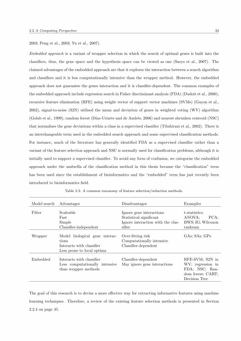
2.2 A Computing Perspective 32
2003; Peng et al., 2003; Yu et al., 2007).
Embedded approach is a variant of wrapper selection in which the search of optimal genes is built into the
classifiers, thus, the gene space and the hypothesis space can be viewed as one (Saeys et al., 2007). The
claimed advantages of the embedded approach are that it explores the interaction between a search algorithm
and classifiers and it is less computationally intensive than the wrapper method. However, the embedded
approach does not guarantee the genes interaction and it is classifier-dependent. The common examples of
the embedded approach include regression search in Fisher discriminant analysis (FDA) (Dudoit et al., 2000),
recursive feature elimination (RFE) using weight vector of support vector machines (SVMs) (Guyon et al.,
2002), signal-to-noise (S2N) utilised the mean and deviation of genes in weighted voting (WV) algorithm
(Golub et al., 1999), random forest (Dıaz-Uriarte and de Andres, 2006) and nearest shrunken centroid (NSC)
that normalises the gene deviations within a class in a supervised classifier (Tibshirani et al., 2002). There is
an interchangeable term used in the embedded search approach and some supervised classification methods.
For instance, much of the literature has generally identified FDA as a supervised classifier rather than a
variant of the feature selection approach and NSC is normally used for classification problems, although it is
initially used to support a supervised classifier. To avoid any form of confusion, we categorise the embedded
approach under the umbrella of the classification method in this thesis because the “classification” term
has been used since the establishment of bioinformatics and the “embedded” term has just recently been
introduced to bioinformatics field.
Table 2.3: A common taxonomy of feature selection/reduction methods.
Model search Advantages Disadvantages Examples
Filter ScaleableFastSimpleClassifier-independent
Ignore gene interactionsStatistical significantIgnore interaction with the clas-sifier
t-statistics;ANOVA; PCA;BWS; IG; Wilcoxonranksum
Wrapper Model biological gene interac-tionsInteracts with classifierLess prone to local optima
Over-fitting riskComputationally intensiveClassifier-dependent
GAs; SAs; GPs
Embedded Interacts with classifierLess computationally intensivethan wrapper methods
Classifier-dependentMay ignore gene interactions
RFE-SVM; S2N inWV; regression inFDA; NSC; Ran-dom forest; CART;Decision Tree
The goal of this research is to devise a more effective way for extracting informative features using machine
learning techniques. Therefore, a review of the existing feature selection methods is presented in Section
2.2.4 on page 45.

2.2 A Computing Perspective 33
2.2.2 Validation Mechanism
Assessment of the statistical significance and validation of findings is a critical step in cancer classification
(Ebert and Golub, 2004). The principle of microarray-based classification is to use it as an insight for the
existing data for prediction of future data. As Simon (2003) said: “We want to be able to predict class
membership for future samples whose class membership we do not know”. However, the major problem
of the existing classification methods is the over- or under-fitting problem, which is due to the nature of
microarray data, such as high gene dimension, sample scarcity and complex interaction between genes within
the data; the structure of the classification framework, such as data preprocessing prior to classification that
may homogenised the primary features and the secondary or the less important features; complex hybrid
classification model, such as DT/SVM (Statnikov et al., 2004); and high network size in the ANN model
(Chen et al., 2007). Thus, methods for obtaining an unbiased assessment on the classifier’s error rate are
required. These methods, ideally, assess one or more of the following factors (Simon et al., 2003; Somorjai
et al., 2003; Dabney, 2005):
• The unbiased estimation on the prediction accuracy in which high classification corresponds to low
misclassification errors (Classification Accuracy).
• The practicality of the prediction model dealing with the data characterised by high feature dimension
and sample sparsity (Scaleability and Generalisability).
• The interpretability of the prediction models based on the complexity of the hybridised approach to
reduce computational cost and to minimise the risk of over-fitting (Simplicity).
• The interpretability of the results at a biological level rather than at a statistical significant (Biological
versus Statistical Significance).
The validation techniques in this section, however, evaluate the accuracy and the generalisability of the
classification models in providing statistical-based results rather than biological-based. These techniques
include splitting sample patterns and cross-validation (CV) procedures. Table 2.4 on page 34 shows the
taxonomy of validation mechanism for evaluating classification methods.
The straightforward approach for properly evaluating a classifier is to base the evaluation on a separate set
of test sample data. In a sample-splitting procedure, the data set is randomly split into two independent
subsets, namely training set and test set. The splitting ratio is normally 0.7 : 0.3 in which 70% of the data
is used as a training set and the remaining 30% as a test set. The training set is used by a classifier to
learn discriminant patterns and the test set is used for evaluating generalisability of the trained classifier.
The fundamental principle of this procedure is that the samples in the test set must not have been used in

2.2 A Computing Perspective 34
training the classifier (Ambroise and McLachlan, 2002; Dupuy and Simon, 2007). In fact, some studies use a
third set, known as validation set, to act as a secondary test set, on the quality of the classifier. This method
will prevent the over-fitting problem, providing the data set is large and there are sufficient samples in all
three sets (Cartwright, 2008a).
Another commonly used validation approach is cross-validation (CV). Unlike the sample-splitting procedure,
CV is an iterative process. In each iteration, part of the data set is used to develop a classifier and another
part of the data set is left apart as a validation set to the classifier. Similar to the sample-splitting procedure,
the samples in the validation set must not have been used in training the classifier (Dupuy and Simon, 2007).
The widely used CV approach in bioinformatics literature is leave-one-out cross-validation(LOOCV) due to
the small number of samples available in microarray data (Cartwright, 2008a). For LOOCV, each time the
classifier is trained on the entire samples, with the exception of a single sample that acts as a test for the
trained classifier. The performance of the classifier is then accessed by this exception sample. This is carried
out for all samples in the data set. The main advantage of LOOCV is that it ensures the unbias estimation
on the classification result, however, the downside of LOOCV is that it is computationally intensive. Thus,
it is not recommended if the data sets are large, but, the n-fold cross-validation (CV) procedure is suggested.
In n-fold CV, the data set is divided into n subset of data with equal sized of sample patterns in each fold.
Each time, the classifier is trained using n− 1 subsets of data and tested with the omitting subset of data.
The process repeats for n iteration and each time, a different subset of data is used to evaluate the classifier.
Comparing to LOOCV procedure, n-fold CV is efficient when the sample size is large.
Table 2.4: A common taxonomy of validation mechanism on classification model.
Validation mecha-nism
Description Advantages Disadvantages
Sample-splitting Randomly divides data with the ra-tio of 0.7 : 0.3 in training and testsets, respectively. The training set con-tains adequate information to developthe classifier and the test set is used toevaluate generalisability of the trainedclassifier
Simple and fastLess prone to over-fitting risk
Biased classifica-tion estimationwhen the samplesize is small
Cross-validation Iterative process where the data is ran-domly divided into n folds with equalseized of sample and classifier is devel-oped on the n−1 folds with tested withthe omitting fold
Unbiased classifica-tion estimationLess prone to over-fitting risk
Computationallyintensive when thesample size is large
Most studies in the bioinformatics literature favoured to apply more than one variant of validation mechanism
in their studies. The commonly used combined mechanisms are the sample-splitting and LOOCV procedures,

2.2 A Computing Perspective 35
where the prediction performance of the trained classifier is evaluated using the n-fold CV procedure in the
training set (see Appendix C).
Simon (2003) and Ambroise and McLachlan (2002) discussed several important issues on model evaluation
that have been overlooked by some studies and optimistically bias prediction performances were reported.
2.2.3 Classification Design
At present, the two dominant designs in cancer classification are class prediction and class discovery, each is
used as a different study’s objective. When the study emphasises either the insight exploration of the known
genes or the risk prediction of metastasis activity (survival rate of cancer patients), based on the known
cancer classes, class prediction design is the only option (Khan et al., 2001; Dudoit et al., 2002; Cho et al.,
2003b; Lee and Lee, 2003; Bloom et al., 2004; Liu et al., 2004a,c; Lee et al., 2005). While the objective of
study is to discover the unknown cancer class from the existing cancer classes, the model construction is based
on class discovery paradigm (Golub et al., 1999; Ross et al., 2000). Both approaches are concentrating on
the improvement of classification accuracy rather than other issues. The class prediction approach develops
the predictive strength of the models based on the classification training accomplished with a sequence of
training samples associated with the target output for the training samples. Hence, it is also known as
supervised learning. While the class discovery approach develops the discovery ability of the models based
on the observation of the correlation between samples, that is, genes that are expressed in a similar manner
are grouped in similar clusters, while samples with a low similarity of genes are a distance away. Therefore,
it is known as unsupervised learning in classification literature. Table 2.5 presents a common taxonomy of
classification design with their prominent advantages and disadvantages.
Table 2.5: A common taxonomy of classification design.
Model objective Advantages Disadvantages Examples
Class prediction RobustSimple
Over-fitting riskUnable to generate newknowledgeCurse of data dimensionalityand sparsity
WV; DT; SVM;FDA; KNN; ANN
Class discovery Generate new knowledgeLess prone to over-fitting risk
Computationally intensive HC; K-means clus-tering; SOM
2.2.3.1 Supervise learning
One of the earliest supervised learning methods in microarray classification is weighted voting (WV) classifier
proposed by Golub et al. (1999). The WV algorithm is a linear classifier based on the amount of weight
2.2 A Computing Perspective 36
carried by each vote in participating entities (i.e. genes). Each entity is assigned a weighted vote and the
magnitude of each vote is dependent on the entity value in the sample and the correlation of that entity’s
with the class distinction. The weighted vote of gene g is the production of the subtraction of the normalised
log gene value xg ,with the average mean log gene values of all classes bg and the ratio of mean and standard
deviation of the gene ag based on the measure of signal-to-noise (S2N) ratios. Thus, the formation of the
weighted vote of a gene can be expressed as WVg = ag(xg − bg). The WV algorithm has been commented
on, as computationally simple and ability to select genes, however, the downside of this algorithm is that it
is designed for binary classification with a lack of exploration on gene dependency.
Golub et al. (1999) applied WV classifier to categorise the new unknown samples of acute leukaemia cancer
based on the top-50 informative genes identified by S2N ratios. They observed that satisfactory classification
results were achieved with 29 out of 34 test samples being correctly classified. However, Dudoit et al. (2000)
commented that an incorrect variance calculation in S2N ratios decreased the efficacy of WV algorithm.
Dudoit et al. developed a univariate selection approach based on the ratio of mean and variance of the genes
for cancer classification.
The classification tree, also known as decision tree (DT), is another commonly used classifier in microarray
studies (Liden et al., 2002; Li et al., 2004; Lee et al., 2005). A DT contains a set of internal nodes and
leaf nodes in which the internal nodes associated with splitting criterion (i.e. splitting features and split-
ting predicates of the features) and the leaf nodes represent individual classes (Lu and Han, 2003). The
construction of the tree involves two phases: growing phase and pruning phase. In growing phase, the tree
is constructed by splitting each feature and its predicates into individual internal nodes to learn a set of
general rules in class separability. Once the rules have been learned, pruning phase begins by pruning the
tree with an IG function to reduce the entropy caused by over-partitioning samples into leaf nodes and to
avoid an over-fitting problem. The claimed advantage of the classification tree is that it is easily understood
by the user.
Liden et al. (2002) proposed three types of rule induction criteria to improve the performance of DT, namely
divide-and conquer (DAC), boosting and separate-and conquer (SAC) based on LOOCV procedure. DAC is a
variant of recursive partitioning technique that used IG to select branching features in generating hierarchical
rule sets on the tree, boosting is an ensemble method that used iteratively readjusts the weight distribution
of the training samples and SAC is the covering method that iteratively finds one rule that covers a subset of
the data rather than recursively partitioning the entire data set. They observed that a DT trained with the
boosting technique outperformed DAC and SAC approaches, however, there is no significant improvement
in binary classification comparing it to other classification methods, such as SVMs, clustering approach and
Bayesian approach using 128 genes. For multiclass classification, a boosting classification tree showed 100%

2.2 A Computing Perspective 37
classification accuracy based on about 20 rules regardless on the number of genes. They also observed that
the boosting approach works significantly better in a classification tree rather than decision stumps. This
observation has also been noted by Dudoit et al. (2002) and Lee et al. (2005) when they applied classification
and regression tree (CART) in binary and multiclass cancer classification.
Despite combining a DT with aggregation methods (i.e. boosting and boostrap), Statnikov et al. (2004)
combined the DT with SVMs for multiclass cancer categorisation. They observed that a sole classification
tree performs significantly worse than other supervised methods, such as SVMs, KNNs and ANNs, regardless
with or without the selection method. Li et al. (2004) also observed that the selection method downgraded
the performance of a DT, due to the tree being built by dynamically selecting the most informative features
from the data set and selection method, in fact, it removes features from the data set and some informative
features may be lost during the data removal process. They used the J48 tree algorithm that was implemented
in WEKA environment to discriminate multiclass tumour data.
Fisher’s discriminant analysis (FDA) is also widely used for microarray classification. FDA is a non-
parametric method, that finds an optimal projection matrix (gene subsets) which reshapes the data set
for maximum class separability using the ratio of between-class to within-class matrices (BSS/WSS) (Lu
and Han, 2003). Unlike linear discriminant analysis, FDA has the ability to discriminate multiclass data,
but, its predictive efficacy is dependent on the number of features in the data set and it ignores the correlation
between features (Dudoit et al., 2000).
Dudoit et al. (2000, 2002) compared discriminative ability of FDA with four other supervised methods,
namely KNN, linear discriminant analysis (LDA), DT trees and aggregating classifiers for binary and multi-
class scenarios. They observed that generalisability of FDA is dependent on gene dimension and sample size.
The performance of FDA was significantly improved with a smaller number of genes used for classification.
A similar pattern of discriminant methods and observations are also reported by Lee et al. (2005) when
they extended the comparison studies with more variations of classification methods, microarray data and
selection techniques.
Meanwhile, Cho et al. (2003b) utilised the kernel function to enhance the capability of FDA for multiclass
classification. They observed that the kernel-based FDA has better classification results in a multiclass
scenario than in a binary classification. They reported the minimum overall mean errors of 0.96% and 4.06%
based on 5-fold cross-validation (CV) procedure on multiclass and binary microarray data, respectively.
Naive Bayes (NB), is another supervised classifier that can, generally, achieve good classification perfor-
mance in most application areas and some bioinformatics areas, including bioassay classification and clinical
diagnosis. However, it is not a popular method to be implemented in microarray classification because it is
a univariate-based approach. A NB classifier is a statistical-based approach based on the elementary Bayes’

2.2 A Computing Perspective 38
Theorem with strong independence assumptions, i.e. all members (i.e. samples or genes in the context of
microarray data) in the data set are unrelated to each other. Given a C number of classes in the data set
and s is an observation (i.e. a sample or a gene) in the data set with a known probability density of the class
p(Sc). If the class prior probability p(c) is known, then the posterior probability P (c|s) of the observation
can be expressed as:
P (c|s) =p(Sc)
p(S).L
p(Sc). (2.1)
L is the predefined number of labelled observations (priori) used to measure the likelihood of the observation,
irrespective of their class labels. The main advantage of the NB classifier is due to its over-simplified assump-
tions which often work efficiently in classification problems, however, this simplicity is also the drawback of
the NB classifier when identifying correlated set of genes in the microarray data.
In microarray literature, the NB classifier is normally implemented for binary classification problems, rather
than for multiclass scenarios, or is used as the performance evaluator in logistic regression model (LRM).
Hwang et al. (2002) implemented the NB classifier to discriminate between two types of acute leukaemia
classes. Chu et al. (2005) used the Bayes’ Theorem to evaluate the significance level of the genes identified
by the Gaussian methods in three binary microarray data sets and Li and Yang (2002) used the Bayesian
information criterion (BIC) in LRM to determine the minimal number of genes to be needed for a discriminant
microarray analysis.
k-nearest neighbour (KNN), on the other hand, is a similarity-based approach based on the minimum distance
measure between the testing samples and the training samples (Lu and Han, 2003). For KNN, k number
of training samples (i.e. nearest neighbours) are used to label unknown samples according to the distance
measure. For instance, if k = 1, the test sample is simply assigned to the class of its nearest neighbour
(training sample), if k > 2, then the test sample is assigned to the nearest class with the minimum distance.
The distance metric can be any similarity measure statistics such as Pearson correlation, Euclidean distance,
Spearman correlation and many more. The common advantages of KNN are that it is computationally
simple, less prone to noise and bias, however, it is not scaleable and is similar to FDA, its performance is
reliant on the number of k points used in the classification process (Lu and Han, 2003).
Dudoit et al. (2000, 2002) performed a comparison study between KNN with four other supervised methods,
i.e. FDA, LDA, DT and aggregating classifiers based on binary and multiclass scenarios. They observed that
the classification performance of KNN is improved when the number of classes is not large and KNN performs
remarkably well compared to DT and aggregating methods, albeit, with a lack of transparency. Li et al.
(2004) also found that the KNN classifier outperforms DT in ensemble classification. They indicated that the
choice of feature selection methods will, in fact, affect the performance of KNNs in the multiclass scenarios.
2.2 A Computing Perspective 39
However, Golub et al. (1999) argued that the performance of classification methods could indeed be based
on the types of expression data when they applied KNN to discriminate genes that are uniformly high in
one class and uniformly low in the other, for binary cancer classification. Wang et al. (2006) observed that
the interaction between genes in microarray data were not explored by KNN based on a leukaemia cancer
classification conducted using the LOOCV procedure and a lymphoblastic origin sample misclassified into
myelogenous origin.
Meanwhile, Li et al. (2001a,b) applied GA to select informative genes for KNN for leukaemia cancer clas-
sification. They claimed that hybrid GA-KNN is superior to KNN, simply because the hybrid approach
implicitly assumes that genes are similarly expressed within each type of sample group, however, this could
be problematic when subtypes of cancer exist, resulting in the relevant genes not being uniformly expressed
in the group. Ooi and Tan (2003) also commented that the GA-KNN strategy might not be optimal for
multiclass scenarios due to the identified genes being based on the n top-ranked genes that were picked from
a finite number of gene predictor sets, resulting in little exploration on gene interactions which are believed to
be more complex for multiclass scenarios. Furthermore, the distance metrics used to determine the k neigh-
bours became less sensitive, as data dimensional increases and sample data might also be unclassifiable, if
no satisfactory majority vote was obtained from the k neighbours.
Artificial neural network (ANN) is the commonly used machine learning approach for clinical diagnosis and
it has recently received attention in the bioinformatics field. ANN is a non-parametric method that inter-
connects numerous artificial neurons (i.e. genes) and processes information using connectionist computation.
For ANN, all incoming signals are processed by neurons in the layer and the output signal is forwarded to
neurons in the next layer. The predictive strength of ANN can be accelerated by the parameter choices
including activation function, learning algorithm, momentum and bias on the gene selection. The common
example of supervised-based ANN is a multilayer perceptrons network that contains three layers of neurons,
using the backpropagation learning algorithm.
Bloom et al. (2004) applied a 3-layered ANN with backpropagation learning to classify multiclass sample
data based on the genes selected using H-test statistic, for two different array platforms, i.e. cDNA and
oligonucleotide. They reported a mean test accuracy of 83% and 88% based on a 95% confidence interval for
cDNA and oligonucleotide platforms, respectively and, a mean test accuracy of 85% in combining platforms.
Meanwhile, Ko et al. (2005) compared ANN with two other supervised methods, i.e. DT and KNN for a
multiclass scenario. They also reported that ANN outperforms DT and KNNs based on purity estimation
values for network structure of 61-10-21.
Despite using multiple layer networks, Khan et al. (2001) proposed a single-layered ANN for predicting
4-class of SRBCTs tumours based on 96 gene expression signatures selected by the PCA. They reported

2.2 A Computing Perspective 40
100% classification accuracy based on test data with no evidence of over-fitting. Due to the encouraging
results reported by Khan et al., their work has been extensively studied by other researchers (Wei et al.,
2004; Chen et al., 2007). Wei et al. used a 3-layered ANN with 10-3-1 structure to predict the survival rate
of neuroblastoma (NB) patients based on DNA clones selected by PCA, while Chen et al. adopted 40-3-4
structure to diagnose and classify SRBCT tumours using the genes selected based on multiplex RT-PCR
assays. Markowetz and Spang (2005), however, commented that perfect separation can be an artifact of high
dimension rather than an indication of a biological relationship of genes, in fact, it is a sign of over-fitting.
Keedwell and Narayanan (2003) also used a single-layered ANN for acute leukaemia and myeloma microarray
classification based on gene combinations selected by GA. Their work was further extended using only a
single-layered ANN to identify gene combinations (Narayanan et al., 2005). In the latter work, myeloma
data was pruned from the original 7129 genes to only 21 genes based on 3 network models. The first
two models were used to reduce the gene dimension, while the third model was used for classification. They
reported 98.1% overall accuracy based on test sample data using See5 tool. When data partitioning approach
was applied on the models, 29 genes were reported.
Liu et al. (2004a) examined generalisability of ensemble ANNs, based on three selection methods, which are
Wilcoxon ranksum, PCA and t-test, to improve predictive accuracy and robustness of ANNs. Three ANN
models, each accommodating different selection methods, were used to train the same set of training sample
data and the overall mean accuracy from these models was calculated. The bootstrap technique was used to
re-sample the data 100 times, resulting 300 ANN models for each data set. They claimed that the ensemble
ANN method performed better, or, is at least comparable, to bagging tree classification.
Schwarzer et al. (2000) discussed several important issues on the improper implementation of ANN which
might led to serious consequences in the classification results and they have reported some important common
mistakes that have been omitted in the reported results.
Support vector machine (SVM) is another machine learning technique that has recently received attention in
the bioinformatics field. It was originally introduced by Vapnik and his co-workers for data mining problems
(Lu and Han, 2003). SVMs adopt the structure risk minimisation principle to identify a hypothesis that
can guarantee the lowest probability of error (Lee et al., 2005). The underlying principle of SVM is to
map the features to a higher dimensional space using a linear function and to identify the maximum-margin
hyperplane, i.e. a linear line that can separate samples into two distinct classes. The common advantages of
SVM are that it explores gene interactions, scaleable to high dimensional and robust performance, however,
a significant drawback is that it is designed for binary classification. The suggested solutions to the problem
are either to breakdown the multiclass problem into several binary scenarios, or to iteratively performing
binary classification until all classes have been separated (Lu and Han, 2003). However, these suggestions are

2.2 A Computing Perspective 41
computationally intensive. To reduce the computational cost of SVMs, two weighting strategies are proposed
for multiclass problems, i.e. one-versus-all (OVA) and all-pairs (AP). The OVA approach builds k number
of linear SVMs corresponds to k number of classes in multiclass data and distinguishing one class at a time
from all the other classes, while the AP approach distinguishes two linear SVMs from the rest of the classes
at one time. Additionally, different kernels applied to different data sets can also improve the classification
performance of SVM (Cruz and Wishart, 2006).
Guyon et al. (2002) introduced RFE selection in SVM algorithm to find the optimal gene subset for binary
classification. They revealed that the classification results are significantly affected by types of selection
methods, rather than by classification methods, based on cross test results obtained with a WV classifier
and FDA classifier. However, Li et al. (2004) argued that the accuracy of classification is dependent on
the choice of the classification methods rather than on selection methods. They made their comment based
on the evaluation of eight different selection methods constructed using the RankGene algorithm and four
supervised classification methods on multiclass microarray data.
Peng et al. (2003) applied AP strategy in linear SVMs for each binary classification ramified from a multiclass
data set and these results are then combined to form the final result for a multiclass data set based on the gene
subsets derived from GA’s selection. They observed that the combination of GA and SVM bestows benefit
to microarray analysis, including avoiding over-fitting, no priori information on the data set is required and
robust to noise. Better performance on GA/AP-SVM is reported compared to KNN, HC and SVM trained
with a OVA strategy. Similar hybridisation of GA and AP-SVM also reported by Liu et al. (2005a) and
unlike Peng et al. who used RFE to further eliminate the non-predictive features in the GA-derived gene
set, Liu et al. used NSC to refine the GA-derived gene set.
Yeang et al. (2001) compared AP and OVA weighting strategies based on the multiclass classification. They
noticed that the performance of strategies is dependent on the number of genes defined in the classification
process. The AP approach outperforms the OVA approach when a fixed number of genes is applied, however,
the OVA approach achieves lower error rates than the AP approach in a LOOCV procedure when a random
number of genes is applied. In contrary, Li et al. (2004) commented that the performance of weighting strate-
gies appeared to be problem-dependent and they made their comment based on the experiments conducted
on eight multiclass microarray data.
Meanwhile, Shen and Tan (2006), attempted to improve the performance of SVMs using various selection
methods, such as BSS/WSS ratios, partial least squares (PLS) and PCA, however, the improvement is not
significant.
Instead of refining weighting strategies, some research focuses on the implementation of nonlinear kernel
functions on SVMs. For instance, Lee and Lee (2003) developed Gaussian-based kernel function on multiclass

2.2 A Computing Perspective 42
scenarios and presented promising results when the data sets were appropriately preprocessed with adequate
selection methods; Statnikov et al. (2004, 2005) used polynomial function to evaluate the performance of AP
and OVA strategies; and Mao et al. (2005) applied fuzzy-based kernel function in microarray classification.
Class prediction has been extensively studied in literature. For instance, Boulesteix et al. (2008) reviewed
various statistical aspects of supervised classifier evaluation and validation, such as accuracy measures,
error rate estimation procedures, selection methods, choice of classifiers and validation strategy. Kotsiantis
(2007) reviewed various supervised learning classification techniques that cover the major theoretical issues
and possible bias combinations of the techniques. Markowetz and Spang (2005) discussed four supervised
learning methods, i.e. likelihood-based methods, DTs, SVMs and regularised binary regression, based on
model selection and over-fitting perspectives. Meanwhile, Simon (2003) discussed the key factors to be
observed in developing diagnostic and prognostic prediction models based on microarray data and the pitfalls
to be aware of in reading reports of microarray-based studies. The statistical issues that arise from the use
of microarrays are addressed by Simon et al. (2003). Cruz and Wishart (2006) conducted a detailed review
of published studies employing machine learning methods for cancer prediction and prognosis, focusing on
the key aspects of the types of methods being used, the types of integrated training data, the kinds of
endpoint predictions being made, the types of cancers studied and the overall performance of the methods in
predicting cancer susceptibility. Table 2.6 presents a unified view of supervised learning methods reviewed
in this section.
2.2.3.2 Unsupervised learning
One of the earliest unsupervised learning methods in microarray studies is hierarchical clustering (HC).
HC organises data into a hierarchical tree structure according to the proximity matrix such as Manhattan
distance or Euclidean distance, and the result is depicted in a binary tree, known as a dendrogram (Xu
and Wunsch, 2005). The root node of the dendrogram represents the entire data set and each leaf node
is regarded as a data object (i.e sample) containing information of cluster formation and the correlation
between clusters. Two common strategies for constructing dendrograms are the agglomerative (bottom-up)
and the divisive (top-down) approaches (Jiang et al., 2004). For the agglomerative approach, the dendrogram
is overgrown in a massive structure and then pruned layer-by-layer by merging the two closest clusters at
each step, until a predefined number of clusters are obtained. The divisive approach, conversely, starts with
one cluster containing all data objects and at each step, a new cluster is created. The main advantage of
the HC algorithm is due to its ability to graphically represent the data set which provides a global view of
the distribution of data. However, it is not robust and is computationally intensive (Xu and Wunsch, 2005;
Jiang et al., 2004). Zhang et al. (2006) also commented that the HC algorithm is not as robust as the SVM,

2.2 A Computing Perspective 43
Table 2.6: A unified view of supervised learning methods. The * indicates the performance of classifier in dealingwith specific task and is range from * (represents poor performance) to *** (represent best performance)
Task WV DT SVM FDA KNN ANN
Strategy Vote weight-ing
Entropyfunction
Maximum-margin
Maximum-likelihood
Similar prox-imity
Perceptron
Generalisability ** * *** ** ** ***
Missing valuehandling
* ** ** * * *
Noise handling * ** ** * ** **
Model trans-parency
** *** * ** * *
Multiclass han-dling
* ** ** ** ** ***
Feature selec-tion
distance ma-trix
backward/forwardsearch
weight vec-tor
forwardsearch
distance ma-trix
entropyfunction
Genes interac-tion
* ** *** * * ***
a supervised learning method, in producing an unbiased estimation of predictive power for new unknown
sample data based on the splice recognition problem.
Ross et al. (2000, 2004) and Alizadeh et al. (2000) used the HC algorithm in analysing the variation of gene
expression patterns for both binary and multiclass scenarios. For Ross et al. (2000), the HC algorithm is
used to group 60 cell lines of an anticancer drug screen (NCI60) with similar repertoires of expressed genes
and to group genes whose expression level varied among the cell lines in a similar manner. They conducted
the experiments twice using different gene subsets to ensure the robustness of the analysis results and the
proximity similarity of genes was computed using the Pearson correlation coefficient. Meanwhile, Alizadeh
et al. applied the HC algorithm for lymphoid malignancies clustering based on the basis of the similarity
in the pattern with which the expression varied over all samples. Ross et al. (2004), however, developed a
2-dimensional HC algorithm to discover a new sub-cluster of an acute myeloid leukaemia cancer.
K-means clustering is another unsupervised approach based on gene partition and centroid adjustment
principles. For K-means clustering, the cluster centroid value is iteratively adjusted each time when a gene
is introduced so that the distance between genes within a cluster can be minimised using a proximity matrix.
The K-means clustering algorithm commented on, as a fast algorithm converges with a small number of
iterations, however, this feature tends to lose out with high gene dimension and noisy data (Jiang et al.,
2004). Xu and Wunsch (2005) commented that the iteratively optimal cluster centroids on K-means cannot

2.2 A Computing Perspective 44
guarantee convergence to a global optimum, moreover, K-means clustering is sensitive to outliers and noisy
data. Even if a gene is located far away from the cluster centroid, it is still forced into a cluster and thus,
distorts the cluster shape (Xu and Wunsch, 2005).
The Kohonen’s self-organising map (SOM) is an ANN model based on unsupervised learning paradigm.
It is a single-layer mapping algorithm in which input and output neurons (i.e. genes) are organised in a
two-dimensional map (matrix). Each neuron is associated with a reference vector and each gene point in
the matrix is mapped to the neuron with the nearest reference vector (Jiang et al., 2004). The training
process of SOM commented on, is more robust than K-means in dealing with high noisy data, however, it
requires a predefined number of clusters and the grid structure of the neuron map (Jiang et al., 2004). In
addition, SOM may suffer from input space density misrepresentation in which low pattern density genes
may be ‘buried’ by high pattern density genes (Xu and Wunsch, 2005). In this case, SOM is not effective
because most of the interesting patterns that merge into only one or two clusters and cannot be identified
(Jiang et al., 2004).
Golub et al. (1999) applied binary SOM to automatically cluster acute leukaemia microarray data on the
basis of the 6817 gene expression patterns. They observed that SOM was effective, although not perfect, for
class discovery with 34 of 38 test samples correctly classified. Wang et al. (2003), however, used SOM to find
the optimal map neurons, that can represent the configuration of the input tumour data, and this optimal
map was used to classify tumour samples and identify informative genes using fuzzy C-means clustering, a
variant of K-means, and pair-wise based FDA.
Jiang et al. (2004) and Xu and Wunsch (2005) presented comprehensive literature on the clustering algo-
rithms. Jiang et al. compared three clustering categories in gene expression, i.e. gene-based, sample-based
and subspace clustering methods, as well as the problems pertinent to each clustering category. Xu and
Wunsch reviewed clustering approaches for data sets appearing in statistics, computer science and machine
learning.
Microarray classification has been extensively reviewed over the last decade. For instance, Mocellin and
Rossi (2007) presented the principles underlying the analysis of microarray data, such as cancer classification,
microarray data collection and normalisation, gene expression comparison and clustering algorithms. Valafar
(2002) conducted a survey on the techniques that have been used in mining microarray data, including
missing values imputation, selection approach and clustering method. Lu and Han (2003) presented a
comprehensive overview on cancer classification and selection methods, along with an assessment based on
aspects such as computation time, classification performance and the ability to reveal biologically meaningful
gene information. Kuo et al. (2004) also outlined the main challenges and critical considerations regarding the
construction of classification models in gene expression studies, such as modelling techniques and biological

2.2 A Computing Perspective 45
validation of results. Asyali et al. (2006) reviewed class prediction and class discovery that are applied to
gene expression data, along with the implications of the findings. Tarca et al. (2007) conducted a survey on
the supervised and unsupervised learning methods in the application to biology, along with the methods and
examples implemented in the open source data analysis and visualisation R language. Dupuy and Simon
(2007) discussed the dispute between microarray-based clinical research and published microarray studies
in which gene expression data is analysed in relation to cancer outcomes. They proposed guidelines for
statistical analysis and reporting based on the common discrepancies identified.
2.2.4 Feature Selection (FS)
A known challenge in microarray studies is to identify smaller sets of informative genes that are highly
associated with the pathogenesis condition of malignancy proliferation from high feature dimension of data.
Thus, FS techniques are normally expected in the preprocessing stage. FS is the process of finding a subset of
the original features of a data set, either individually correlated or combinatory correlated, and run on data
containing only these features, generates a classifier with the highest possible accuracy. Some FS methods
have the ability to remove redundant information from microarray data, thus, it is also known as feature
reduction in literature. Several claimed advantages of FS include (Saeys et al., 2007; Rocha et al., 2007):
• To provide a focus group of genes that are useful in either biological or classification way.
• To avoid the over-fitting risk and to improve the prediction accuracy of classifiers.
• To provide faster and cost-effective models.
• To reduce the complexity of the classification model.
Table 2.3 on page 32 presents the taxonomy of FS along with its advantages and disadvantages.
2.2.4.1 Filter selection
Filter selection measures the marginal relevance of the individual feature to the known class with standard
statistics criteria and is independent of the classification model used. Although the filter selection is simple
and efficient, however, it overlooks the relationships between features. Pruning these correlated features in
the preprocessing stage seem unimportant, when individually evaluated, but, are crucial for explaining the
problems when more than one of these features are taken into consideration.
The simple filter scheme is to compute a mean and a variance, or a standard deviation in the data. For
instance, Dudoit et al. (2000) proposed between-group/within-group (BSS/WSS) ratio based on mean and

2.2 A Computing Perspective 46
variance computation between selected features with the known class which is expressed as below:
BSS(j)
WSS(j)=
∑i
∑k I(yi = k)(xkj − xj)2∑
i
∑k I(yi = k)(xij − xkj)2
, (2.2)
where xij denotes value of feature j for sample i, xj indicates overall mean value of feature j across all
samples in the data set, xkj indicates average value of feature j for its class k and I is indicator function in
the ratio. Dudoit et al. (2002) commented that the use of a feature variance value in filtering features is more
accurate and efficient than using standard deviation of the feature. They made such comments based on the
comparison study with S2N ratios proposed by Golub et al. (1999). However, BSS/WSS is not scaleable to
high dimension and is sensitive to data magnitude and as a result, feature reduction and normalisation are
generally expected to preprocess the data. For instance, Dudoit et al. (2002); Lee and Lee (2003) preprocessed
acute leukaemia oligonucleotide data with steps involving thresholding, filtering, log-transformation and
normalisation based on a variance, to remove data redundancy and suppress value magnitude before the
implementation of BSS/WSS ratios. Meanwhile, Shen and Tan (2006) preprocessed GCM oligonucleotide
data and lymphoblastic leukaemia oligonucleotide data by computing a standard deviation in the data and
statistic approaches, such as PCA and PLS for feature reduction. Lin et al. (2006), however, attempted to
use BSS/WSS ratios to reduce the dimensionality space of genes for NCI60 oligonucleotide data and GCM
data which have been preprocessed by zero mean normalisation.
More complex filter selection methods include the use of statistics functions, including PCA and PLS for
redundancy reduction and feature extraction (Khan et al., 2001; Cho et al., 2003a; Liu et al., 2004a; Wei et al.,
2004; Tan et al., 2005; Shen and Tan, 2006), the use of information gain (IG) matrices to rank features (Cho
and Won, 2003), the use of proximity matrices, such as Euclidean distance, Pearson correlation, Spearman
correlation and Cosine correlation for feature extraction (Cho and Won, 2003, 2007), the use of t-test and
F-test in selecting important features (Inza et al., 2004; Liu et al., 2004a; Mao et al., 2005; Tan et al., 2007)
and many more. Amongst these methods, PCA is commonly applied to microarray data.
The principal component analysis (PCA) is a profoundly statistical model implemented in the chemoinfor-
matics field (Gasteiger, 2006; Brown, 2009) that finds a set of orthogonal principal components, i.e. features,
based on the eigenvector concept to describe the correlation of sample data in different independent variables
and is an effective approach for redundancy reduction without the loss of data characteristics. However, this
may be its drawback from a classification point of view because there is no guarantee that the principal com-
ponent representing the large variance in an independent variable would necessarily be the component most
strongly related to the dependent variable (Tan et al., 2005). Unlike PCA, the partial least squares (PLS)
maximises the sample covariance between the linear combination of dependent features and the orthogonal

2.2 A Computing Perspective 47
component of independent features (Tan et al., 2005), thus, the relationships between features are taken into
consideration in the pruning process.
2.2.4.2 Wrapper selection
A wrapper selection method conducts the selection process with an optimisation algorithm that searches the
space of possible feature subsets to find the best subsets of features based on the predictive error estimation
returned by a supervised classifier. A typical wrapper approach based on the hybrid GA/ANN is presented in
Figure 1.3a on page 11. The idea of wrapper selection is to “wrap” the classifier in an optimisation algorithm
that would make a feature subset from the current set of features. This feature subset will continue to grow
until the accuracy of the model was no longer more accurate (Kohavi and John, 1997). An objective function
is generally defined for wrapper selection that takes into consideration different criteria, such as the accuracy
of a classifier that is trained in the feature subset. The number of features to reward the model or the
predictive performance of the trained classifier is evaluated by using a separate set of unknown data samples.
Wrapper selection does not have the possible shortcomings of filter selection, however, wrapper selection
easily over-fits the data and is computationally intensive. In addition, wrapper selection is dependent on the
‘wrapped’ classifier, thus, there is no guarantee that an optimal feature subset for one classifier will be the
optimal for another classifier.
The evolutionary algorithm (EA) is commonly used selection method to “wrap” the classifier to find cor-
related gene subsets in microarray data. An EA algorithm normally involves two search processes, i.e.
exploration and exploitation. The former process conducts a global search (i.e. heuristic search) on data
space for possible regions of feature subsets and the latter process exploits the favourable feature subsets
from the region space in which the possible subsets of features are retained using an exhaustive search. The
examples of EA include genetic algorithm (GA), simulated annealing (SA) and genetic programming (GP).
EA has been studied in bioinformatics literature as an optimisation algorithm for efficient classification and
gene subset selection. Li et al. (2001a,b) used GAs to select an arbitrarily fixed set of 50 and 40 genes for colon
and lymphoma cancer classification, respectively, using a consensus KNN classification method. Meanwhile,
Deutsch (2003) developed a replication algorithm based on EA with a KNN classifier and better classification
accuracy and smaller gene subsets used in the classification were observed. A similar approach is also used
by Jirapech-Umpai and Aitken (2005) on acute leukaemia and NCI60 oligonucleotide data. They evaluated
the generalisability of a classifier based on separate test sets and a variation of the number of selected genes
for classification. Ooi and Tan (2003), on the other hand, used an EA with a maximum likelihood classifier
for multiclass scenarios and they defined the objective function based on the independent test error rate
returned by the classifier. Liu et al. (2005a) and Peng et al. (2003) also applied similar approaches as used

2.2 A Computing Perspective 48
by Ooi and Tan (2003), however, instead of using a maximum likelihood classifier, they used SVM as the
classifier. They used LOOCV procedure as an objective function. The validation of their work is based on a
single test sample for each data set. Tan et al. (2007) also used SVM as a classifier in their work, however,
instead of using LOOCV as objective function, they applied multiobjective functions in EA, i.e. to maximise
the classification accuracy of the feature subsets and to minimise the number of features selected, based on
multiple feature subsets produced by multiple feature selection methods. However, there may be a risk of
an over-fitting of their results due to an over-pruning of the data and the high complexity of the proposed
model.
In addition to conventional classification methods, perceptron-based classification is also proposed with
consensus of GA. Keedwell and Narayanan (2003) used a single-layered ANN as a classifier to discover small
combinations of genes which lead to the correct classification for acute leukaemia and myeloma data. Similar
ANN architecture is also used by Cho et al. (2003a) and Karzynski et al. (2003). Cho et al. defined the
objective function based on the prediction results returned by ANN with a 3-fold cross-validation procedure
and they evaluated the generalisability of the classifier with a separate blind test set and a variation of the
number of selected genes for classification. Meanwhile, Karzynski et al. used GA to find the population of
optimal solutions for ANN architecture in where the balance between samples and parameters to train is
optimal. Bevilacqua et al. (2006a) and Lin et al. (2006) proposed the use of error estimation returned by
the ANN classifier as the objective function in the classification of breast cancer metastasis recurrence and
multiple microarray data, respectively. Bevilacqua et al. (2006a) observed that GA/ANN hybrid model is a
robust algorithm and would only be affected by a very low variability of results due to the efficacy of GA to
focus its search on feature subsets and to avoid local minima entrapment.
2.2.4.3 Embedded selection
Embedded selection is the latter variant of wrapper selection in which the search procedure is built in and
is specific to a classification model. Unlike wrapper selection, embedded selection does not guarantee the
findings of correlated feature subsets, however, it is being far less computationally intensive than wrapper
selection.
The simple scheme of embedded selection is a univariate-based approach that selects features using a mean
and a standard deviation computation in the data, such as signal-to-noise (S2N) ratios developed by Golub
et al. (1999) for a WV classifier. Given gene g in class c, in order to classify gene g, the mean µ and the
standard deviation σ of gene g in class c are computed. [µ1(g), σ1(g)] and [µ2(g), σ2(g)] denotes the means
and the standard deviations of the log of expression levels of gene g for the samples in class 1 and class 2,
2.2 A Computing Perspective 49
respectively. The S2N can thus be expressed as:
S2N = P (g, c) = |µ1(g)− µ2(g)
σ1(g) + σ2(g)|. (2.3)
For S2N ratios, large value indicates a strong correlation between gene expression and the distinction class,
while the sign of S2N being positive or negative corresponds to gene g being more highly expressed in class
1 or class 2, respectively. Golub et al. (1999) used S2N ratios to select a fixed set of 50 genes, 25 genes for
each known cancer class, in acute leukaemia data and they observed a satisfactory validation of the results
was achieved in a blind test.
S2N ratios are normally used as a comparison study with other embedded selection methods and supervised
classification methods. Takahashi et al. (2005) compared the number of identified marker genes by S2N
ratios with projective adaptive resonance theory (PART) for acute leukaemia data and they observed that a
total of 10 informative genes is sufficient for classification rather than using 50 genes for class discrimination.
Dudoit et al. (2002) compared the statistics criteria of S2N with BSS/WSS ratios and they concluded that
the use of the deviation computation is unstable compared to the use of variance computation.
Recursive feature elimination (RFE) is another embedded selection method that assists in improving the
classification accuracy of SVMs as proposed by Guyon et al. (2002). RFE was inspired by backward feature
elimination in which the removal of multiple irrelevant features by iterating three steps: train SVM, rank
features and removes the feature with the smallest rank, each time only one least-fitted feature is removed.
RFE is a univariate-based approach that finds an individual feature using the ranking criterion of optimal
brain damage (OBD) algorithm. The OBD algorithm approximates the changes in cost function δJ(i) by
expanding cost function J in the hyperplane. The δJ(i) can thus be expressed as follow:
δJ(i) =∂J
∂wiδwi +
∂2J
∂w2i
(δwi)2, (2.4)
where wi is the weight vector for feature i, J = |w|2/2 for linear SVM computation and the weight vector
can be computed with the following expression:
w =
Ns∑i=1
αiyixi, (2.5)
where Ns is the number of support vectors which are defined with 0 < αi ≤ C, C is the penalty parameter
for the error xi and yi are data instances in a d-dimensional Euclidean space. For linear SVM, the margin
width can be set to 2/||w||. At the optimum of J , the first order can be neglected and the second order

2.2 A Computing Perspective 50
becomes ∂J(i) = (∂wi)2. As removing the feature i, means ∂wi = wi, the second order w2
i is taken as the
ranking criterion. By iterating the processes of training SVM, adjusting cost function and removing the
smallest weight vector, a smaller set of features with higher weight vectors is yielded.
Guyon et al. (2002) used RFE to find a small subset of genes for acute leukaemia and colon data. They
reported only 2 genes are required for acute leukaemia classification without a validation mechanism, however,
a total of 64 genes are necessary for the baseline method to get the best result with a LOOCV procedure.
For colon data, they identified 4 marker genes. Shen and Tan (2006) applied RFE to optimise multiclass
SVMs. The RFE is used to execute each SVM classifier independently to obtain the best performance and
the smallest gene subsets. A 3-fold cross-validation is then applied to validate the fitness of the gene subset
for each classifier, so that a set of base classifiers with different gene subsets can be constructed for multiclass
classification tasks.
Forward selection, also known as regression selection, is commonly embedded in linear discriminant methods
and DT. Contrary to RFE selection, forward selection selects one feature at each step, this gives the best
prediction accuracy for FDA and DT classifiers in combination with the previously selected features. Forward
selection for FDA is proceeded as follows (Park et al., 2007):
1. After k features are selected, perform the steps (a) - (c) for the remaining candidate features:
(a) Add one feature to the set of k features already selected.
(b) Perform FDA for the k + 1 features and project data samples.
(c) Measure prediction accuracy in the projected space.
2. Find the k + 1th best feature by choosing the feature which gives the highest prediction accuracy.
3. Repeat the processes to produce gene ranking forwards.
Although forward search is embedded in an FDA classification model, an independent filter selection method
is always applied to an FDA model for better classification. Dudoit et al. (2000, 2002) applied BSS/WSS
ratios to find a smaller set of gene subsets from the data that had been pruned for microarray cancer
classification. Similar approaches were also reported by Lee et al. (2005) for classification in multiclass
scenarios. Meanwhile, Park et al. (2007) used forward selection to identify a number of optimal genes to be
selected for acute leukaemia microarray classification based on different splitting to the training and test sets,
and LOOCV procedure. They observed that it is difficult to determine the number of optimal genes with
LOOCV validation due to the potentiality of over-fitting risk in the training process and different splitting
of the data also gave a different number of optimal genes. They also compared consistency in gene ranking
of forward selection with RFE selection in SVMs and S2N ratios in WV classifier. Based on the top 100

2.2 A Computing Perspective 51
selected genes between different selection methods, they found that forward selection has less than 10% of
common genes among the genes selected by the other two methods.
Nearest shrunken centroid (NSC) was proposed by Tibshirani et al. (2002) for prediction analysis of microar-
rays (PAM) classifier to identify minimal subsets of genes on SRBCT tumour data. NSC shrinks the class
centroids for each gene toward overall centroids for each gene with an absolute value ∆ after standardising
by the within-class standard deviation for each gene. The NSC value is defined as the following equation.
NSC = sign(dik)(|dik| −∆)+, (2.6)
where dik is a t-statistic for gene i, comparing class k to the overall centroid and each dik is reduced by an
amount ∆ in threshold. + means positive part of the t-statistic (if t > 0, then t+ = t, else t+ = 0). To
compute dik,
dik =xik − xi
mk.(si + s0), (2.7)
where xik is centroid for gene i in class k, xi is overall centroids for gene i, si is the pooled within-class
standard deviation for gene i, s0 is a positive constant value and mk is defined as follows:
mk =
√1
nk+
1
n, (2.8)
where nk is sample number for class k and n is all sample number.
Tibshirani et al. (2002) tested different shrinkage parameters in NSC with 10-fold cross-validation and
identified 43 and 21 informative genes based on shrinkage parameters ∆ = 4.34 and ∆ = 4.06 for SRBCTs
and acute leukaemia microarray data, respectively. A high consistency on the selected genes compared to
the original study (Khan et al., 2001) was also reported for SRBCTs data. Dabney (2005) commented that
NSC computation is wrapped with layers of complexity which can be simplified. He criticised the insertion
of ‘fudge factor’ to each t-statistic’s denominator instead of simple t-statistics. A further level of complexity
is added to shrink the class centroids toward their overall mean which is not necessary for gene ranking.
He presented an alternative gene ranking scheme, namely ClaNC, based on the principle of NSC without a
shrinkage or fudge factor component and observed that ClaNC is much simpler and has substantially lower
error rates than NSC.
Feature selection/reduction is a vast topic by itself and has been extensively studied in literature. Saeys
et al. (2007) reviewed the usage of feature selection approaches in existing bioinformatics domains, including
sequence analysis, microarray analysis and mass spectra analysis, as well as upcoming domains such as single

2.2 A Computing Perspective 52
nucleotide polymorphism (SNP) analysis. Meanwhile, Guyon and Elisseeff (2003) presented a wide range
of aspects discerning variable and feature selection in microarray analysis. Park et al. (2007) evaluated
the consistency of three embedded supervised approaches, namely S2N in WV algorithm, RFE in SVM and
forward selection in FDA, in gene ranking under the changes of training samples or different selection criteria.
They concluded that the performance of selection methods are dependent on the number of available samples
and selection criteria, and this data dependency has posed a dilemma between the necessity and reliability of
feature selection in microarray studies. This findings also been noted by Jeffery et al. (2006) when different
sizes of samples and features were tested in multiple binary microarray classification. Meanwhile, Osareh and
Shadgar (2008) commented that the selection methods, especially the filter selection, is strongly dependent
on the size of the selected features rather than the choice of the selection method itself. To alleviate the
data sparsity problem, Saeys et al. (2007) suggested two alternatives which could enhance the robustness
of the finally selected gene subsets: (1) the external evaluation on the selected genes at each stage of the
training process and (2) the use of ensemble selection approaches. Asyali et al. (2006), however, proposed
the use of feature extraction to reduce the gene dimension first, before the application of selection approach.
However, these alternatives may yield an intensive computational cost and the identification of correlated
genes is purely dependent on the choice of selection approaches in ensemble.
Inza et al. (2004), on the other hand, compared six different filter criteria, namely Shannon-entropy, Eu-
clidean distance, Kolmogorov-dependence, Kullback-Leibler, P-metric and t-score for discrete and continuous
data with a sequential forward selection procedure which is a variant of the hill-climbing wrapper search in
colon and leukaemia studies. They observed that the application of a gene selection approach leads to con-
siderably better classification accuracy results in comparison to the non-gene selection approach, moreover,
several common genes have been found in both filter and wrapper approaches which may lead to biological
interpretation, albeit, that further investigation is required. Osareh and Shadgar (2008) also observed a
significant improved classification performance in a supervised classification method with the application of
a gene selection approach. They made such comments based on five supervised classifiers, i.e. SVMs, KNNs,
NB, ANNs and DT; in four filter selection methods, i.e. t-statistics, IG, Relief Algorithm (RA) and PCA.
Asyali et al. (2006) commented that there is no clear distinction between feature selection and feature extrac-
tion in bioinformatics literature as in pattern recognition literature. They argued that PCA, FDA, SOM and
multidimensional scaling are all examples of feature extraction algorithms which have been miscategorised
as feature selection or classification methods and this can lead to a poor diagnostics test and biomarker de-
velopment due to feature extraction algorithms using metagenes (i.e. new genes from the linear combination
of some particular genes) instead of the existing genes in the data. However, their argument has not receive
wide attention from the bioinformatics field. This may be due to the following reasons:

2.2 A Computing Perspective 53
• The output provided by feature extraction is not so biologically different from feature selection. Thus,
the differentiation between these approaches is not important.
• The bioinformatics researchers might not be aware of the difference between feature extraction and
feature selection as both methods are commonly used to solve the dimensionality problem in the field.
For instance, PCA has proven its usefulness in identifying gene expression signatures for diagnosing
SRBCTs tumour (Khan et al., 2001), predicting the survival of neuroblastoma patients (Wei et al.,
2004) and differentiating different groups of primary lung tumours (Wang et al., 2006).
To conclude, majority of the bioinformatics literature is favourable on the filter selection approach. This is
mainly because such approach has been profoundly used in biology experiments and has been scientifically
proven by mathematics scientists on its efficiency in spotting the significance difference between individual
features in the data. With the increased understanding in molecular biology, many unknown areas in the
past have been discovered.
These areas include the gene-gene interactions (i.e. gene regulatory network) in the microarray data, the
gene-gene interactions in different microarray platforms (i.e. cDNA and oligonucleotide), the gene-peptide
interactions (i.e. the association between genes and its protein peptides) and the peptide interactions within
a protein. As a result, the univariate filter selection became obsolete, as it was unable to explore the
interaction between features within the data. The multivariate selection, such as wrapper selection, has
become the primary research in the bioinformatics field. Even so, the univariate filter selection method is
generally expected as a comparison method to the multivariate selection.
2.2.5 Computing Challenges
The advance of computing technology in cancer classification has created a new era for genetic analysis in
the bioinformatics field. However, it also poses some challenges including:
• The lack of understanding of microarray data resulting in an ambiguity of the objectives of the study.
Most existing studies have been misconceived by the usage of a classification method. Microarray
investigation has been biased towards discovery-based research rather than hypothesis-driven research
(Dupuy and Simon, 2007) due to microarray data containing complex interactions between the corre-
lated genes underlying certain biological pathways. Genes with high expression levels in microarrays do
not always underly the biological causes, however, its correlated genes with moderate expression levels
trigger the problems (Markowetz and Spang, 2005). Thus, hypothesis-driven research based optimal
feature sets for classification does not imply that this feature set is highly relevant to the problem
(Kohavi and John, 1997), thus flaws in the results occur.

2.2 A Computing Perspective 54
• The risk of over-fitting and biased under-estimates of the error rate due to the misuse of a validation
mechanism and resubstitution estimation for classification (Simon, 2003; Simon et al., 2003; Markowetz
and Spang, 2005; Dupuy and Simon, 2007). Microarray data has a high gene dimension and small sam-
ple size, thus, n-fold cross-validation and sample-splitting procedures are not appropriate for model
construction and evaluation. Additionally, the construction of a classification model based on genes
selected using all samples in the data set and with no separate set of sample data for validation pur-
pose could lead to an overly optimistic and inflated prediction accuracy. This phenomena is known as
resubstitution estimation, a common error occurred in classification process. Moreover, some studies
presented a dual-validation procedure in which the classifier is validated with a cross-validation proce-
dure and “additional independent samples”, have brought more confusion than clarity to the results
(Dupuy and Simon, 2007).
• The lack of supporting evidence in the declaration of new prediction models. Many prominent studies
made claims for gene expression classifiers and for new classification algorithms based on the invalid
result findings from improper cross-validation (Ambroise and McLachlan, 2002; Simon, 2003; Simon
et al., 2003), an overly complication of the hybridisation of multiple filter selection approaches on two
distinct acute leukaemia specimens by Sethi et al. (2009), selection bias on the selected genes based
on the entire data sets by Osareh and Shadgar (2008), and ambiguous validation approach by Chetty
and Chetty (2009) in classifying multiclass microarray data sets. A feasible solution to the problem is
to conduct a comparative study with other classification algorithms using the same data set and the
same validation mechanisms (Simon et al., 2003).
• The unrealisation of the influence of the model complexity to the prediction results which result in
model over-fitting (Markowetz and Spang, 2005). As Simon (2003) stated: “Complex methods with
large number of parameters often fit the data used to develop the model well, but provide inaccurate
predictions for independent data”. The large parameters in complex models allow them to fit any kind
of problem, but simultaneously, redundant parameters yield confusion in training the classifiers due
to the fact that the classifiers are statistically programmed to learn all parameters in the algorithm
without knowing the usage of the parameters in the study.
• The unrealisation of the effects of data preprocessing in the findings of the relevant information of the
problems. Oligonucleotide microarray data are generally high expression magnitude and most genes are
suppressed (i.e. negative expression levels), thus, data preprocessing is generally expected to provide
a higher prediction accuracy of classifier. As a result, the ‘true’ cancer markers are ‘buried’ by other
higher gene expressions and are omitted from classification.

2.3 Summary 55
2.3 Summary
Over the past decades, vast developments in the medical field, particularly, in molecular diagnosis. The
creation of microarrays to examine genome-wide expression data has provided a global view on the fluc-
tuations of gene expression levels in response to either the physiological alterations or the manipulations
of transcriptional regulators of living systems. Such development provides insight into information of the
interaction of biological behaviour for both normal and diseased tissues which are ultimately important for
the design of an effective treatment therapy for patients.
This chapter presents the relevant literature covering both the biology and the computing perspectives on
microarray studies. The related literature has been reviewed and shows that the research area of microarray
production and marker identification is still immature, as a result, technical aspects pertaining to these two
domains have been exposed. Comparisons on capabilities and limitations for microarray design, selection
techniques, classification methods and validation mechanism are shown in Tables 2.2 - 2.4. The challenges
pertaining to biology and computing communities are also discussed in Sections 2.1.6 and 2.2.5. Four major
points from the literature are summarised as follows:
Gene expression measurements. The variation in gene expression measurements is inevitable due to a
lack of control in microarray production (see Section 2.1.6). Care in every phase of microarray production,
from sample preparation to image analysis, can minimise the impact of these errors but does not completely
prevent them. Thus, errors are generally expected in the finished microarrays.
cDNA microarray handling. The low production cost on cDNA microarrays has led to the inconsistency
of microarray handling in individual research laboratories due to different laboratories adopting different
approaches in conducting microarray experiments (see Section 2.1.6).
Computational Analysis on microarray data. Most existing studies have an ill-conceived hypothesis
in microarray classification by treating it as an ordinary data set (see bullet points 1-4 in Section 2.2.5).
Microarray data is distinct from any clinical correlative studies and statistically-based classification studies
in which a large number of samples are analysed with respect to a limited number of features. Therefore,
attention to the choice of computing methods and the hybridisation of selection techniques, classification
methods and validation mechanism are advisable to minimise the over-fitting problem.
Data Preprocessing. Data preprocessing on oligonucleotide microarray data may result in the suppression
and exclusion of the true cancer markers from the marker identification and the classification process (see
Section 2.2.1 and bullet point 5 in Section 2.2.5).
This thesis describes an intelligent gene extraction method using hybrid GAs and ANNs to efficiently extract

2.3 Summary 56
differentially expressed genes for a specific cancer pathology. Chapter 3 presents the methodology used for
constructing a feature extraction model for this thesis.

Chapter 3
Experimental Methodology
Chapter 1 described the problems pertaining to microarray analysis using a computational algorithm and our
approach to solving them. Related literature on the production of microarrays and the computing methods is
reviewed in Chapter 2, along with the challenges posed to both the biology and the computing communities.
In this chapter, a feature extraction model is designed using machine learning methods to overcome the
computational problems addressed in Section 1.2. The existing GA/ANN hybrid models emphasise effective
classification and overlook the level of complexity of feature extraction and the influence of data preprocessing
of the classification results. The microarray data, specifically the oligonucleotide data, will generally require
data preprocessing techniques, such as to scale down the magnitude of the feature values and to convert
the negative values into positive values, before the computing analysis takes place. Thus, inevitable errors
in gene variability results from such techniques occur. Our approach tackles the problem yielded by the
normalisation process in the data preprocessing stage. The novelty of our approach is its simplicity, as it
follows the Ockham’s Razor principle, which can avoid the risk of gene variability errors that yielded by
data preprocessing techniques that may alter the quality of the data to be analysed by a computing analysis
model. Our approach is referred to the overview as illustrated in Figure 1.3b on page 11.
This chapter contains five sections. Section 3.1 describes the acquisition of empirical data to be used in
supporting the theme of this thesis. Section 3.2 discusses the issues concerning the design and building of
the feature extraction model, taking into consideration the hybridisation of GAs and ANNs techniques, the
model simplicity and the adequacy of the parameters in deriving satisfactory results. Section 3.3 presents
the genomic analysis tool, namely GenePattern, which is used to visualise the gene findings of the model.
Section 3.4 presents the validation mechanism via the NCBI Genbank and the SOURCE search system,
which is used to validate the gene findings of the model. Lastly, Section 3.5 provides a summary of the
chapter and to what follows next in the thesis.
57

3.1 Empirical Data Acquisition 58
3.1 Empirical Data Acquisition
The bloom of the Internet in the 1990s has produced a fully developed bioinformatics field with a massive
cyber-space to store microarray data and allow microarray integration from various sources to improve its
quality. The aim of this thesis is to formulate, from the identified computing-related problems stated in
Section 1.2 on page 7, an innovative feature extraction model, namely Genetic Algorithm-Neural Network
(GANN), for extracting informative and relevant features using GAs and ANNs. Two benchmark microarray
data sets, namely acute leukaemia (ALL/AML) and small round blue cell tumours (SRBCTs), were obtained
from its original public repositories and have been used to examine our model. Due to the different data
format in microarray data set than the ordinary data set as showed in Figure 1.1 on page 4, a specially
written C++ program is used to transpose the microarray data sets. Two designed synthetic data sets
characterised with high feature dimension and small sample sizes in response to the research goal of this
thesis, C++ programming was used. Furthermore, two bioassay data sets were obtained from its original
source to evaluate the generalisation ability and the robustness of our model to handle large, imbalanced
and different data representation data sets.
The summary of the microarray data sets, the synthetic data sets and the bioassay data sets to be used in
supporting this thesis are presented in Table 3.1. Figures 3.1-3.5 present data distributions for each data
set based on the multidimensional scaling (MDS) in two-dimensional R plots. The screen shot to construct
a two-dimensional plot on the R environment is presented in Figure 4.3 on page 97. To avoid any form of
confusion on both the biology and computing fields, the original sample names or descriptions in the data
sets were used in this thesis.
3.1.1 Microarray Data Sets
3.1.1.1 Acute leukaemia (ALL/AML)
The acute leukaemia (ALL/AML) microarray data is a 2-class high-density oligonucleotide data set that was
originally presented by Golub et al. (1999) to evaluate the predictive accuracy of a weighted voting (WV)
classifier based on the marker genes selected using the S2N ratio. This data set contains 72 samples, collected
from patients, both adults and children, and were sourced from peripheral blood specimens and bone marrow
samples, distributed into acute lymphoblastic leukaemia (ALL) and acute myelogeneous leukaemia (AML)
classes. Amongst 72 samples, 47 samples were associated with ALL tumour and the remaining 25 samples
in AML. All samples were prepared using Affymetrix technology and contained 7129 probes for 6817 human
genes.
The ALL/AML data set is available online from the Broad Institute that are in partnership with Harvard

3.1 Empirical Data Acquisition 59
Table 3.1: The summary of the experimental data sets.
Data set Description Objective
Microarray Data
Acuteleukaemia(ALL/AML)
2 classes, i.e. ALL and AML. A total of 72samples in which 47 samples are expressed inALL class and the remaining 25 in AML. Eachsample is associated with 7129 genes.
To identify relevant informative genesunderlying the pathogenesis of acuteleukaemia tumours.
Small roundblue cell tu-mours (SR-BCTs)
4 classes, i.e. EWS, BL, NB and RMS. A to-tal of 83 samples in which 29 samples are ex-pressed in EWS class, 11 in BL, 18 in NB andthe remaining 25 in RMS. Each sample is as-sociated with 2308 genes.
To identify relevant informative genesunderlying the pathogenesis of 4 typesof small round blue cell tumours.
Synthesized Data
Syntheticdata set 1
2 classes, i.e. Class 1 and Class 2. A total of100 samples equally distributed in each class.Each sample is associated with 10000 features.
To determine the minimum parametersetting of the model.
Syntheticdata set 2
3 classes, i.e. Class 1, Class 2 and Class 3. Atotal of 67 samples is distributed with 20 sam-ples in Class 1, 30 in Class 2 and the remaining17 in Class 3. Each sample is associated with5000 features.
To simulate a real-world data set thatcontains a complex level of feature in-teractions, high dimension of noisy dataand inequality distribution of samplessize for each classes in multiclass sce-nario.
Bioassay Data
AID362 2 classes, i.e. active and inactive. A totalof 4279 compounds, i.e. 60 active compoundsand 4219 inactive compounds, and each com-pound is associated with 144 attributes (1.4%minority class).
To identify active compounds forFormylpeptide Receptor Ligand Bind-ing assay
AID688 2 classes, i.e. active and inactive. A total of27189 compounds, i.e. 248 active compoundsand 26941 inactive compounds, and each com-pound is associated with 153 attributes (0.91%minority class).
To identify active compounds for YeasteIF2B assay.
University and its affiliated hospitals, the Massachusetts Institute of Technology and the Whitehead Institute
for Biomedical Research. The data set is free to download from the Broad Institute website (ALL/AML
oligonucleotide microarray data, 2007). The online source contains 7129 genes including 312 expressed
sequence tags (ESTs) in which 59 are control tags.
Figure 3.1 presents the distribution of samples on 2 distinct leukaemia classes. From the plot, 25 AML
samples are scattered distantly with a few samples overlapping in the ALL class. Forty-seven ALL samples

3.1 Empirical Data Acquisition 60
have a rather distinct cluster except that a few samples are distance away from the cluster. The reason for
the spread of ALL samples may be due to the fact that there are 2 different lineages of ALL tumours in
the collected samples, i.e. T-cell and B-cell, which may have similar symptoms but have a distinct genetic
alteration, as is showed in Figure 3.1. Both T- and B-cells are two types of lymphocytes (i.e. white blood
cells) which cause lymphoblastic leukaemia. B-cells make antibodies and T-cells make other infection-fighting
substances. Due to no distinguishing of T- and B-cell ALL samples in the downloaded data set, and to avoid
sample mislabelling, all ALL-related samples are grouped under a generic name, i.e. ALL, despite the genetic
differentiation. Even so, the data set is fairly linearly separated.
(a) The description of 72 samples in the ALL/AML data set. There are 25 AML samples and 47 ALL samples(19 were B-cell ALLs, 8 were T-cell ALLs and 20 unspecified).
(b) A two-dimensional plot on the sample distribution in theALL/AML data set. The coordinates x and y reflect the dis-tance (dissimilarities/similarities) of the samples using the MDSfunction in R Project. The ALL class has a rather distinct clus-ter compared to the AML class and only a few ALL samples aredistance away from the cluster. There are only few overlappedsamples from both classes.
Figure 3.1: The acute leukaemia (ALL/AML) microarray data.
The ALL/AML data set has been commonly used in examining the prediction accuracy of classification
methods and it is, generally, altered in some way to facilitate the classification process, for instance, data
normalisation is generally expected to remove any incompetent information for better classification results.

3.1 Empirical Data Acquisition 61
Table C.1 in Appendix C shows some of the related works in the ALL/AML data set. Meanwhile, some
studies reduced the number of genes to be analysed in the classification process (Dudoit et al., 2000; Lee
and Lee, 2003; Mao et al., 2005). As a result, different conclusions can be drawn from these studies as the
relevant marker genes may be removed at the pruning stage. Culhane et al. (2002) further differentiated
ALL samples according to T-cell and B-cell linkages, and outlined the list of the distinct set of genes for each
linkage class. It is a good intention to provide an insight into the information for these linkages, provided
that there are sufficient samples to draw a firm conclusion. However, it is not feasible in this data set as
only 8 out of 47 ALL samples were labelled as T-cell ALL, while the remaining are labelled as generic ALL.
Due to the rapid development of microarray technology, some gene annotations are no longer supported by
the NCBI Genbank. Therefore, to avoid any sort of confusion, the original annotation will be displayed in
our findings and will be cross-referenced with the SOURCE search system and the NCBI Genbank.
3.1.1.2 Small round blue cell tumours (SRBCTs)
The SRBCTs cDNA microarray data was originally presented by Khan et al. (2001), with the intention of
identifying marker genes that distinguish 4 types of round cell tumours of childhood which often masquerade
as each other using ANN classification models in conjunction with the PCA. This data set contains 88
samples, each associated with 6567 probes that were filtered to 2308 genes. The 4 types of tumours are
Ewing’s sarcoma (EWS), rhabdomyosarcoma (RMS), neuroblastoma (NB) and Burkitt lymphoma (BL) which
are collected from two different biological sources, i.e. cell lines and tissue samples, that were prepared
according to standard NHGRI protocol. Amongst 88 samples, 29 samples were expressed in the EWS class,
25 in RMS, 18 in NB, 11 in BL and the remaining 5 samples were blind tests.
The SRBCTs data set is available online and is free to download from the NHGRI Institute website (SRBCTs
cDNA microarray data, 2007). Due to the high dimension of redundant genes expressed during transcription
process, Khan et al. had reduced the number of genes from the initial 6567 genes to 2308 genes using filtering
technique. Therefore, the online version contains only 2308 genes with 83 SRBCTs-related samples and the
5 blind test samples were not published online.
Figure 3.2 shows the distribution of 83 SRBCTs samples on four known classes in the data set. The SRBCTs
plot is much more complex than the ALL/AML data set as it involves multiple tumours which often react
to similar therapies. From the plot, EWS and RMS classes have a lot of shared features, most probably
because both EWS and RMS sarcomas are connective tissue-related cancers, that cause the proliferation of
mesoderm and they can be treated with similar prescribed drugs. The BL class, meanwhile, has a distinct
cluster rather than other classes, probably as it was collected from lymphocyte cells. RMS class has the
widest spread of the samples due to there being 2 subgroups of RMS tumours in the collected samples, i.e.

3.1 Empirical Data Acquisition 62
embryonal and alveolar, which have similar phenotypical symptoms but with a distinctive genetic alteration.
The plot also showed that both the sarcoma-related samples and NB samples were scattered distantly. This
might be due to these samples were collected from different biological sources. Unlike the other, BL samples
were all collected from cell lines. Some related works on the data set is presented in Table C.2 in Appendix
C.
(a) The description of 83 samples in the SRBCTs data set. There are 11 BL cell lines samples, 29 EWS samples (16were tissue samples, 11 were cell lines and 2 unspecified), 18 NB samples (14 were cell lines and 4 were tissue samples)and 25 RMS samples (10 were cell lines and 15 were tissue samples).
(b) A two-dimensional plot on the sample distribution in the SR-BCTs data set. The coordinates x and y reflect the distance (dis-similarities/similarities) between samples using the MDS functionin R Project. The BL class has a distinct cluster compared tothe other classes. The RMS class has the widest spread of thesamples, as well as the NB class. The EWS and RMS classes havea lot of common features as both EWS and RMS are connectivetissue-related cancers.
Figure 3.2: The small round blue cell tumours (SRBCTs) microarray data.
3.1.2 Synthetic Data Sets
To evaluate the performance of GANN and to ensure the desired set of features to be identified, two synthetic
data sets were created using the C++ programming to assess the integrity of GANN in performing a task.
Thirty features were predefined on each data set. All feature values excepting the predefined features, were
standardised with zero mean (µ = 0) and unit standard deviation (δ = 1). The 30 predefined features on

3.1 Empirical Data Acquisition 63
each data set were assigned with different µ values, ranging from 0.5 - 2.0.
3.1.2.1 Synthetic data set 1
The synthetic data set 1 is a 2-class data set that contains 100 samples equally distributed in each class.
For the synthetic data set 1, each sample is associated with 10000 features. Amongst the 30 predefined
features, indexed from 1-15 and 5001-5015 were standardised with the mean value of 2 (µ = 2.0). Similar
to the ALL/AML data set, the synthetic data set 1 can be linearly separated and does not contain complex
feature interactions. Figure 3.3 presents the sample distribution of the synthetic data set 1. This data set
is designed to simulate the gene interactivity pattern of ALL/AML data set and is used to determinate the
minimal parameter setting of our model.
Figure 3.3: A two-dimensional plot on the sample distribution in the synthetic data set 1. The coordinates xand y indicate the distance (dissimilarities/similarities) between samples using the MDS function in R Project.
3.1.2.2 Synthetic data set 2
The synthetic data set 2, as plotted in Figure 3.4, contains 67 samples distributed into 3 distinct classes,
with 20 samples for class 1, 30 samples for class 2 and the remaining 17 samples for class 3. This data
set is designed to simulate the complex feature interactions in the multiclass scenario that contains a high
dimension of irrelevant information and inequality distribution of sample patterns available for each class.
For the synthetic data set 2, each sample contained 5000 features. Amongst the 30 predefined features,
indexed from 1-10 were standardised with the mean value of 0.5 (µ = 0.5) and the remaining 20 features,
indexed from 11-30 were standardised with µ = 2. Similar to the SRBCTs data set, this data set has a
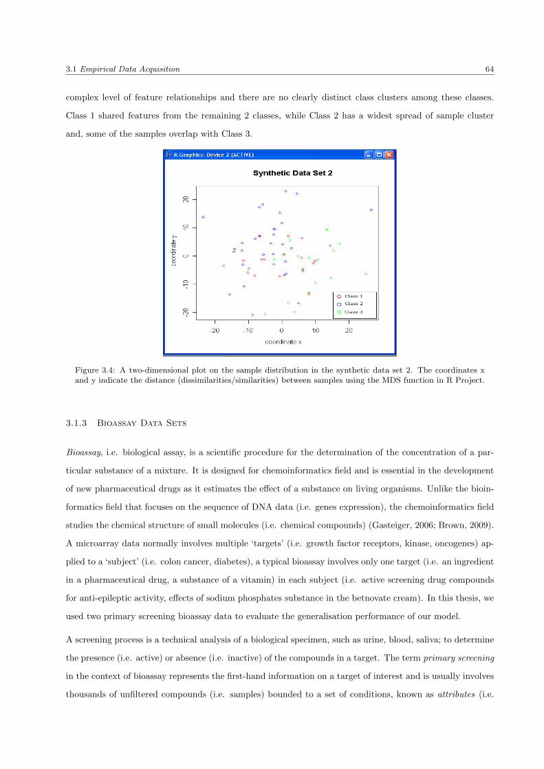
3.1 Empirical Data Acquisition 64
complex level of feature relationships and there are no clearly distinct class clusters among these classes.
Class 1 shared features from the remaining 2 classes, while Class 2 has a widest spread of sample cluster
and, some of the samples overlap with Class 3.
Figure 3.4: A two-dimensional plot on the sample distribution in the synthetic data set 2. The coordinates xand y indicate the distance (dissimilarities/similarities) between samples using the MDS function in R Project.
3.1.3 Bioassay Data Sets
Bioassay, i.e. biological assay, is a scientific procedure for the determination of the concentration of a par-
ticular substance of a mixture. It is designed for chemoinformatics field and is essential in the development
of new pharmaceutical drugs as it estimates the effect of a substance on living organisms. Unlike the bioin-
formatics field that focuses on the sequence of DNA data (i.e. genes expression), the chemoinformatics field
studies the chemical structure of small molecules (i.e. chemical compounds) (Gasteiger, 2006; Brown, 2009).
A microarray data normally involves multiple ‘targets’ (i.e. growth factor receptors, kinase, oncogenes) ap-
plied to a ‘subject’ (i.e. colon cancer, diabetes), a typical bioassay involves only one target (i.e. an ingredient
in a pharmaceutical drug, a substance of a vitamin) in each subject (i.e. active screening drug compounds
for anti-epileptic activity, effects of sodium phosphates substance in the betnovate cream). In this thesis, we
used two primary screening bioassay data to evaluate the generalisation performance of our model.
A screening process is a technical analysis of a biological specimen, such as urine, blood, saliva; to determine
the presence (i.e. active) or absence (i.e. inactive) of the compounds in a target. The term primary screening
in the context of bioassay represents the first-hand information on a target of interest and is usually involves
thousands of unfiltered compounds (i.e. samples) bounded to a set of conditions, known as attributes (i.e.

3.1 Empirical Data Acquisition 65
features). Due to the majority class of inactive compounds in the primary screening bioassay data, the
number of false positives (FPs), i.e. misclassification of an inactive compound as an active compound, are
enormous. This led to the implementation of selection methods to identify the most significance of attributes
that can efficiently discriminate between the active and the inactive compounds in bioassay data sets. A
typical bioassay data set contains two generic classes, i.e. active (i.e. positive) and inactive (i.e. negative),
and tends to be large and highly imbalanced, i.e. the ratio of 1 active compound to 1000 inactive compounds
(Schierz, 2009).
Many selection methods were applied to reduce the number of attributes in the data set. However, not
many selection methods are capable to select the most significant attributes from a bioassay data set, mainly
due to the multiple data representation in the data set and the data are highly imbalanced. Many of the
methods have considered only qualitative information (Brown, 2009) of the data set, i.e. active or inactive
of an attribute against a particular compound (binary value), but not the quantitative information of the
data set, i.e. the concentration level of a particular compound (real number).
In this thesis, two virtual bioassay data sets, namely AID362 and AID688, were used to assess the gener-
alisability of our model in handling highly imbalanced data which containing multiple data representation,
as well as the extraction capability of our model in finding quantitative attributes from the bioassay data.
These data sets were originally introduced by Schierz (2009) to study the efficiency of the cost-sensitive clas-
sifiers, i.e. Naive Bayes (NB), Support Vector Machine (SMO), C4.5 Tree (J48) and Random Forest, that
were developed on the WEKA environment, to identify active compounds in the data sets. The summary
of the data sets is presented in Table 3.1 on page 59.
3.1.3.1 AID362
The AID362 data set is a relatively small data set in the context of bioassay that details the results of
a primary screening bioassay for Formylpeptide Receptor (FPR) Ligand Binding assay. It contains 4279
compounds, i.e. 60 active compounds and 4219 inactive compounds, with a ratio of 1 active compounds to
70 inactive compounds (1.4% minority class) and 144 attributes. Amongst 144 attributes, 3 were presented
in integer numbers, 27 were real numbers and the remaining 114 were binary numbers. Figure 3.5 presents
the compounds distribution of the AID362 data set.
3.1.3.2 AID688
The AID688 data set is a large data set that details the results of a primary screening bioassay for Yeast
eIF2B assay. It contains 27189 compounds, i.e. 248 active compounds and 26941 inactive compounds, with
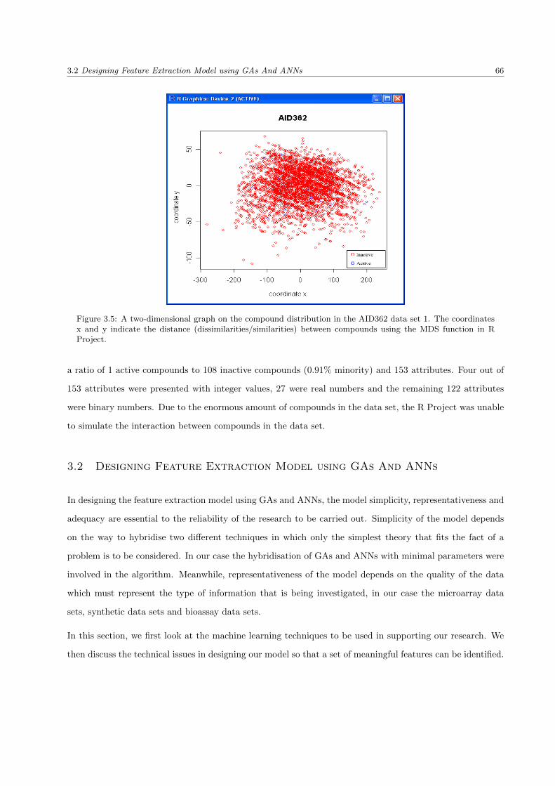
3.2 Designing Feature Extraction Model using GAs And ANNs 66
Figure 3.5: A two-dimensional graph on the compound distribution in the AID362 data set 1. The coordinatesx and y indicate the distance (dissimilarities/similarities) between compounds using the MDS function in RProject.
a ratio of 1 active compounds to 108 inactive compounds (0.91% minority) and 153 attributes. Four out of
153 attributes were presented with integer values, 27 were real numbers and the remaining 122 attributes
were binary numbers. Due to the enormous amount of compounds in the data set, the R Project was unable
to simulate the interaction between compounds in the data set.
3.2 Designing Feature Extraction Model using GAs And ANNs
In designing the feature extraction model using GAs and ANNs, the model simplicity, representativeness and
adequacy are essential to the reliability of the research to be carried out. Simplicity of the model depends
on the way to hybridise two different techniques in which only the simplest theory that fits the fact of a
problem is to be considered. In our case the hybridisation of GAs and ANNs with minimal parameters were
involved in the algorithm. Meanwhile, representativeness of the model depends on the quality of the data
which must represent the type of information that is being investigated, in our case the microarray data
sets, synthetic data sets and bioassay data sets.
In this section, we first look at the machine learning techniques to be used in supporting our research. We
then discuss the technical issues in designing our model so that a set of meaningful features can be identified.

3.2 Designing Feature Extraction Model using GAs And ANNs 67
3.2.1 GA - An optimisation search method
GAs are optimisation methods, in the context of machine learning, that have their inspiration in the analogy
of biological evolution. The GA as a search algorithm operates on the basis of a population of potential
solutions, rather than a search from general-to-specific solutions or from simple-to-complex. GAs generate,
over time, successor solutions by repeatedly mutating and recombining parts of the best currently known
solutions (Mitchell, 1997b) with the assistance of the mechanics of selection and natural genetic mechanism.
The quality of the solutions in the population will be calculated using a fitness function. For instance, if
the learning task is to formulate a treatment strategy for thyroid dysfunction patient, then the GA’s fitness
could be defined as the number of time a thyroid effective plans that had successfully cured the patient and
the risk of side effects of the plans. Over decades, different techniques were implemented in GAs, however,
they typically share and iterate the following five processes:
1. Establish the population containing a finite number of potential solutions to the problem.
2. Evaluate individual solutions in the population according to the fitness function.
3. Generate a new population by selecting the most fit solutions from the population.
4. Create new solutions by applying genetic operations.
5. Replace current solutions with new solutions if necessary.
In order to construct a GA search model, the following five technical aspects are considered:
1. A way of representing potential solutions to a problem, as individuals, that can be manipulated by
evolutionary mechanism (population).
2. A fitness function that can be used to assess the quality of individuals in solving the problem.
3. A method to select better individuals to create a new generation (selection).
4. A mechanism for genetic change so that the individuals in a new generation will not be identical with
the individuals in the current generation (crossover & mutation).
5. A way of encoding individuals into the computer environment (encoding scheme).
3.2.1.1 Population of potential solutions
A GA population contains solutions that can be constructed as a chromosome which contains all the infor-
mation needed to describe the problem. The individual unit from which each chromosome is constructed is

3.2 Designing Feature Extraction Model using GAs And ANNs 68
referred as genes that represent a unique characteristic to the problem. For instance, if the learning task is
to formulate the treatment strategy for thyroid dysfunction patients, the chromosome that defines a possible
solution to the problem could be formed from the considerations: patient age, phenotypic symptoms, gender,
brain neurotransmitters’ activities, the hormonal activities and the neuropeptides activities.
The size of a GA population and the chromosomes are normally fixed, as a result, the existing chromosome
in the population has to be removed when a new chromosome is introduced by a GA. Cartwright (2008b)
commented that the success of a GA does not critically rely on the exact size of the population provided
that the population is not unreasonably small. However, it relies on the evolution of solutions which only
occurred in GA generations. Too small or too large a population makes proper evolution become impossible
and leads to computational cost problems. Cartwright suggested the ideal population size, in most problems
applied, should be in the range of 40 − 100 and this will lead to a fast convergence of the solution and is
computationally time effective. However, DeJong and Spears (1991) discovered that the choice of population
size had a strong interactive effect on the evolution operator, the crossover operator to be specific, even
after augmenting the crossover operators. With smaller population sizes, crossover productivity effects were
drastic and caused chromosomes to become homogeneous more quickly. With larger population sizes the
crossover productivity effects are far less dramatic. This is due to a lack of information capacity of a smaller
population size which provides accurate sampling. As a result, the optimum solution to the problem may
be overlooked in the process of initialising the population.
To validate the implication of the population to the efficiency of a GA to perform the task, we examined 3
population sizes and the findings were presented in Chapter 5.
3.2.1.2 Fitness of potential solutions
Most real-world problems are multifaceted and full of trade-offs, several factors contributing to measure the
quality of each potential solution in the population can easily be conflicting and it is not always easy to
distill them down to a single factor (Cartwright, 2008b). For instance, if the learning task is to learn a
strategy for playing chess, the quality of the solution can only be based on a single factor, i.e. the number of
games won by the individual when playing against another individual. However, if the task is to formulate a
treatment strategy for thyroid dysfunction patient, the quality of the solution could not be based on a single
factor, instead, multiple factors should be considered, such as the duration of treatment (time element), the
current state of immunological activity of the patient (health condition element), the usage of treatment
preparations (preparation element) and the cost of treatment (financial element). These factors, in most
cases, are conflicting, such as a trade-off between prescribed drugs for patients who have depression as a side
effect with the natural preparations, as the prescribed drugs deteriorate the depression symptoms, although

3.2 Designing Feature Extraction Model using GAs And ANNs 69
the prescribed drugs provide effective effects in patients; and the treatment duration for natural preparations
are much more longer than prescribed drugs, but its have lower side effects.
In the GA, the quality of a chromosome in solving the problem is computed using a fitness function which
yields a quantitative measure on how close the individual units in a chromosome to the desired solution
that is not defined by GA, instead, it is decided by the use upon a suitable relationship for each problem.
For the task to formulate a treatment strategy, the fitness function will include a component that scores the
progression estimation of each treatment stage using the historical records of the patient, along with any side-
effect problems related to the patient. Normally, the GA fitness function rewards the better chromosomes
with a higher fitness value than the poorer chromosomes so that the better chromosome can be further
processed by the evolutionary mechanism and has a better chance of survival in the next generation.
Recent research has concentrated on improving GA fitness functions with either the use of a penalty function
(Beasley et al., 1993; Busetti, 2001) or the incorporation of machine learning algorithms (Li et al., 2001b;
Bevilacqua et al., 2006b; Lin et al., 2006), however, most research is biased towards classification problems
and a trade-off of the computational time and/or the algorithm complexity for a better classification accuracy,
is generally to be expected.
In our approach (see Section 3.2.3 for detailed explanation), we keep as minimal parameter settings as
possible in our model and we defined our model’s fitness function as the number of correctly labelled samples
in the data sets.
3.2.1.3 Selecting potential solutions
The selection process begins when the fitness has been calculated for all individual solutions in the population.
Generally, the selection process is partially stochastic and biased towards better chromosomes in order that
the GA can move forward. This is because if the selection was completely deterministic, the population
would soon be dominated by the fittest chromosome and would quickly become homogenous before the
desired solution is reached (Cartwright, 2008b). This phenomenon is known as premature convergence.
However, if the solution did not have some guidance for selecting a fitter chromosome, the search would be
largely random and the selected chromosome might not be the fittest chromosome, instead, it could be the
poorest chromosome in the population. The process will then further deteriorate in subsequent evolutionary
operations. Two widely adopted selection mechanism in a GA are the roulette wheel and the tournament
selection.
Roulette wheel selection, also known as proportionate selection, ranked the GA chromosomes based on their
fitness proportions in the current population. For roulette wheel selection, every individual chromosome is

3.2 Designing Feature Extraction Model using GAs And ANNs 70
assigned a slot, sized on the proportion of its fitness, on a virtual board. The better chromosome, normally,
has a larger slot than the poorer chromosome. The wheel is then spun and the chromosome, into whose
slot the virtual ball falls, is copied into the parent pool, i.e. the repository in which the chromosomes
have a chance to mate. The selection process is repeated to pick the complement chromosomes until the
parent pool is full. Roulette wheel selection leads to the fast convergence of chromosomes with larger fitness
proportions being more likely to be picked than those chromosomes with smaller proportions, however, it
cannot guarantee that the selected chromosomes are optimal. In addition, roulette wheel selection lacks
stochastic power as the population is easily dominated by fitter chromosomes which, consequently, leaves
an insufficient resource for the genetic mechanism to further exploit the population, resulting in the loss of
better chromosomes being found.
Tournament selection, on the other hand, ranked the GA chromosomes based on the competition basis of at
least two or more chromosomes. For a typical tournament selection, two chromosomes are randomly chosen
from the population and compared. The chromosome with the greater fitness is selected and copied into the
parent pool. The selection process is repeated, to yield a group of competent chromosomes in the parent pool.
Since the tournament selection randomly picks chromosomes, the consequent results may vary each time the
process is performed and fitter chromosomes may participate more than once in the competition. Even so,
tournament selection often yields a more diverse population than roulette wheel selection (Mitchell, 1997b)
and it leads to deeper exploitation of the chromosome search. A known benefit of tournament selection is
that it provides a certain level of confidence of the selected chromosome being fitter than those not being
picked. In addition, it also guarantee that the poorest chromosome will never be selected. The downside of
this method is that it takes a longer time to identify fitter chromosomes than roulette wheel selection.
Cartwright (2008b) noticed that both roulette wheel and tournament selections have a lack of stochastic
features, as a result, neither can guarantee that the best chromosome, in the current generation, will be
chosen again in the next generation. Therefore, a new hybrid-based selection was introduced to overcome
the pitfall of roulette wheel and tournament selections, i.e. stochastic remainder selection.
Stochastic remainder selection is a hybrid method that combines a stochastic element with a deterministic
step to ensure that the best chromosome in the current generation is never overlooked in the next generation.
In stochastic remainder selection, the fitnesses of chromosomes are scaled in accordance with the average
chromosome fitness of 1.0 (Cartwright, 2008b). Each chromosome is copied into the parent pool and the
number of copies is based on the integer part of the average fitness. The fitness of the chromosome is then
subtracted from the average fitness and yields a residual fitness value which must be below 1.0. A modified
roulette wheel or tournament selection is then performed using these residual values to fill the remaining
space in the parent pool. The deterministic step in the stochastic remainder selection ensures that every

3.2 Designing Feature Extraction Model using GAs And ANNs 71
chromosome with a fitness above 1.0 will appear at least once in the parent pool.
Goldberg and Deb (1990) criticised that by using suitable adjustment of selection parameters, except the
roulette wheel selection, a similar performance can be achieved with most selection methods, thus, there is no
absolute better selection method in the GA. They made such observations based on four different selection
schemes: roulette wheel, tournament selection, fitness ranking and steady state selection.
In our design, to avoid the poorest chromosome being selected into the next generation and to prevent the
premature convergence in our model, we chose the tournament selection. Additionally, we also applied the
elitism strategy to retain fitter chromosomes in the parent pool.
3.2.1.4 Evolving the potential solution
The selection method in GAs can only introduce the existing chromosome to the parent pool or remove the
chromosomes from the parent pool, however, it is unable to create new chromosomes for the next generation.
Therefore, a mechanism is required to modify the existing chromosome by introducing “new life” into the
population. Two GA operators that are able to create new chromosomes are crossover and mutation.
A crossover operator is the main operator for generating new chromosomes from existing chromosomes.
There are three common ways of performing crossover: single-point, two-point and uniform crossovers, as
showed in Figure 3.6. For single-point crossover, two chromosomes from the parent pool are each cut at
the same corresponding point and exchange the section after the cut point to produce new chromosomes as
offspring of the parents. Meanwhile, the two-point crossover is very much like single-point crossover, except
that two cut points instead of one are performed. For two-point crossover, the offspring are produced by
swapping the intervening cut points between two parents. Uniform crossover radically differs from single-
and two-point crossovers. In uniform crossover, many small sections rather than a single large block are
swapped between parent chromosomes. The exact swapping points are determined by a crossover mask
which contains a list of random binary values generated every time for each pair of parents.
Uniform crossover is simple, but could be severely disruptive and the degree of disruption critically relies
on the crossover mask (i.e. a defined string used to determine the cut points on the parent chromosomes)
rather than the defining length of the chromosome as single- and two-point crossovers does. Therefore
the crossover mark, in general, is on average one half of the chromosome length which avoids unnecessary
disruption (Cartwright, 2008b). On the other hand, uniform crossover is also likely to break up any large
building blocks in the parent chromosomes and, in some cases, it could be too destructive for a highly
correlated group of individual units in the chromosome. Therefore, it is more effective when applied to
problems which involve only a limited correlation between genes, probably, one or two places apart in the

3.2 Designing Feature Extraction Model using GAs And ANNs 72
Figure 3.6: Three common crossover operators for GAs. These operators form the offspring of chromosomesrepresented by real number encoding. The crossover operators create two descendants (offspring) from twoparents, using the predefined cut points or the crossover mask to determine which parent contributes which bits.
chromosome. Goldberg (1989) observed that multiple cut points, except the two-point crossover, could lead to
the over-interaction between similar chromosomes at the premature stage of convergence, although Syswerda
(1989) argued in favour of uniform crossover. Syswerda argued that uniform crossover is beneficial when the
ordering of genes in the chromosomes is entirely irrelevant and less disruptive with longer defining length
chromosomes. DeJong and Spears (1991) pointed out that the increased disruption of uniform crossover
could be an advantage if the population size is small.

3.2 Designing Feature Extraction Model using GAs And ANNs 73
In crossover operation, the probability that a chromosome selected from a parent pool is determined by a
crossover probability, pc. The pc rate is normally large, typically in the range of 0.6 − 1.0 (Beasley et al.,
1993; Busetti, 2001) so that most, and possibly all, chromosomes in the parent pool are selected for mating.
In the process of chromosome evolution, the crossover operator is responsible for introducing new chro-
mosomes to the next generation only by shuffling genes between parent chromosomes. As a result, the
population is soon flooded by homogeneous chromosomes and becomes stagnated before the desired solution
is found. Therefore a mutation operator which creates new information to the chromosomes is required.
A mutation operator acts as a “background” operator in the evolution process and is responsible for providing
a small diversity in the population when most chromosomes are identical to prevent genetic drift caused by
the accumulation of stochastic errors on each generation. Mutation refreshes the population by inserting a
new value into a small fraction of chromosomes. However, not all new introduced values are beneficial to
the population. This is because mutation does not have a ‘blueprint’ on what so-called ‘good’ information
and ‘bad’ information is. It simply changes the values by randomly picking the fraction of the chromosome.
As a result, some researchers claimed that mutation does not improve the evolution progress but prolongs
the convergence process, because it may destroy important information, by inserting unwanted information
into the chromosome. Therefore, it is important to apply mutation cautiously, this is normally at a low rate
specified by the mutation rate, pm, typically 0.001 (Beasley et al., 1993).
The aim of this research is to identify the informative genes that underly the tumourigenesis pathway of a
specific cancer, i.e. the genetic pattern of tumour formation and tumour production. Therefore, we used
the single-crossover operator in our model to minimise any form of disruption that yielded by the crossover
operator.
3.2.1.5 Encoding evolutionary mechanism
In early work, GA chromosomes were encoded using binary coding that involves only 1s’ and 0s’. With
the rapid development of computer technology, most problems, nowadays, are full of complications and
contradictions which require better ways to encode the problems. Binary coding became obsolete, as it had
a small binary length, which is insufficient to express the present problems. In addition, binary coding has
added complexity in manipulating chromosomes in the evolution process, although it can be easily solved
by applying an additional programming execution rule. Nevertheless further problems arise when the degree
of complexity of the problems are increased, binary coding does not have an adequate length of coding to
express problems and it is far more difficult to interpret than other alternative forms of coding such as real
number representation, which can accommodate far more complicated problems.
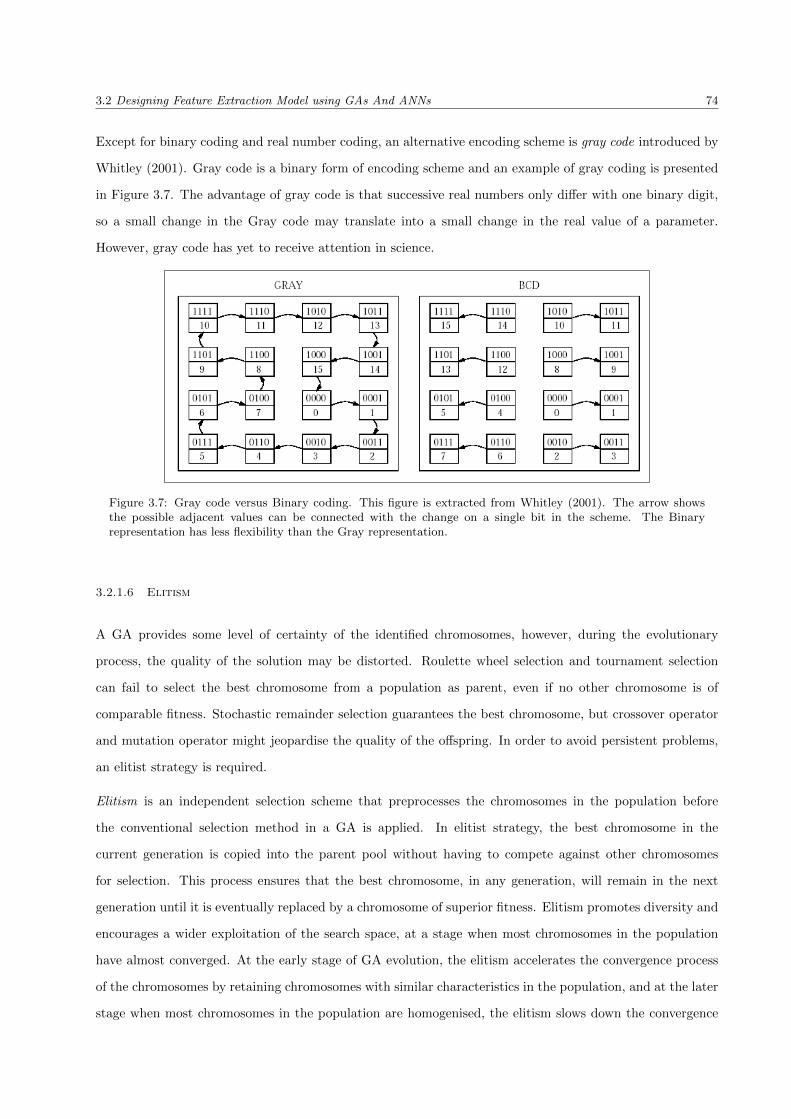
3.2 Designing Feature Extraction Model using GAs And ANNs 74
Except for binary coding and real number coding, an alternative encoding scheme is gray code introduced by
Whitley (2001). Gray code is a binary form of encoding scheme and an example of gray coding is presented
in Figure 3.7. The advantage of gray code is that successive real numbers only differ with one binary digit,
so a small change in the Gray code may translate into a small change in the real value of a parameter.
However, gray code has yet to receive attention in science.
Figure 3.7: Gray code versus Binary coding. This figure is extracted from Whitley (2001). The arrow showsthe possible adjacent values can be connected with the change on a single bit in the scheme. The Binaryrepresentation has less flexibility than the Gray representation.
3.2.1.6 Elitism
A GA provides some level of certainty of the identified chromosomes, however, during the evolutionary
process, the quality of the solution may be distorted. Roulette wheel selection and tournament selection
can fail to select the best chromosome from a population as parent, even if no other chromosome is of
comparable fitness. Stochastic remainder selection guarantees the best chromosome, but crossover operator
and mutation operator might jeopardise the quality of the offspring. In order to avoid persistent problems,
an elitist strategy is required.
Elitism is an independent selection scheme that preprocesses the chromosomes in the population before
the conventional selection method in a GA is applied. In elitist strategy, the best chromosome in the
current generation is copied into the parent pool without having to compete against other chromosomes
for selection. This process ensures that the best chromosome, in any generation, will remain in the next
generation until it is eventually replaced by a chromosome of superior fitness. Elitism promotes diversity and
encourages a wider exploitation of the search space, at a stage when most chromosomes in the population
have almost converged. At the early stage of GA evolution, the elitism accelerates the convergence process
of the chromosomes by retaining chromosomes with similar characteristics in the population, and at the later
stage when most chromosomes in the population are homogenised, the elitism slows down the convergence

3.2 Designing Feature Extraction Model using GAs And ANNs 75
process by introducing chromosomes with different characteristics into the population. Therefore, it reduces
the disruption which may be caused by mutation during the evolutionary process.
3.2.1.7 Exploration versus Exploitation
For an efficient search in GAs, two contradictory search techniques are generally required to find a global
maxima (optimal peak): exploration (performed by crossover and mutation operators) to investigate new
and unknown areas in the search space and exploitation (performed by selection operator) to make use of
information (knowledge) found in the previous points will help in finding better points within a region space
(Beasley et al., 1993). A balance between both techniques are vital in identifying optimal results, thus, a
trade-off between these two techniques must be wisely judged when applied to the problem.
Holland (1992) showed that a well-balanced ratio between exploration and exploitation can be found in
a GA using a k-armed bandit analogy (evolving from a traditional slot machine with a tradeoff between
exploitation of a lever that has the highest expected payoff and exploration to get more information about
the expected payoffs of the other levers). However, Beasley et al. (1993) questioned the practicality of
the assumptions made by Holland. A commonly found problem is genetic drift which is caused by the
accumulation of stochastic errors, which result in a gene becoming predominant in the population, as once
a gene has converged in this way, it is fixed. This produces a domino effect, as generations go by, each gene
eventually becomes fixed (Beasley et al., 1993). The impaction of genetic drift to a GA could be beneficial
if the predominant gene is what is being look for, however, it can become disastrous if the population is
dominated by the wrong gene.
Beasley et al. (1993) suggested the rate of genetic drift can be reduced by increasing the mutation rate to
explore more unknown peaks in the space. However, excessive mutation could lead to a poor exploration of
the region space and high computation processing. This produces skewed results in GAs.
There are no standards or guidelines for balancing the powers of exploration and exploitation in a GA. The
efficiency of a GA to find an optimal solution is mainly reliant on the trial-and-error experiments conducted
with different GA’s parameters and sufficient number of evolution (i.e. fitness evaluation) provided to the
chromosomes. Therefore, in our design, we examined various sizes of fitness evaluations to determine the
best balance ratio between exploration and exploitation of a GA.
3.2.2 ANN - A universal computational method
An ANN is a computational model that attempts to simulate the structure and/or functional aspects of
the human brain in the way that an individual biological neuron reacts in pattern recognition. In the

3.2 Designing Feature Extraction Model using GAs And ANNs 76
human brain, it is the combined efforts of numerous neurons acting together to create complex behaviours,
while in the ANN, it mirrors the structure of the human brain in which many simple processing elements,
known as nodes, acting as neurons, work co-operatively. As a consequence, ANNs are often referred to as a
connectionist model, in the context of machine learning.
An ANN contains numerous nodes that are interconnected using connection links which are associated with
different connection weights that are arranged in layers (see Figure 3.8). The initial connection weights for
constructing ANN are given random values as the network does not have prior knowledge for modelling the
problem. The learning process then takes place, during which the network is shown with a large number of
examples that are required to learn, and in response adjusts its connection weights in order to give meaningful
results. A network in which all the weights have been determined is considered as fully trained and is ready
for use. The training process of ANN is shown in Figure 3.9.
Figure 3.8: A typical 3-layered ANN.
Each ANN node is featured by a set of connection weights, an activity level that determines the polarisation
state of a node, an output activation value and a bias value, each represented mathematically by real numbers.
The connection weight can be positive (i.e. excitatory) or negative (i.e. inhibitory), and determines the effect
of the incoming signal on the activity level of the node. The input signals, generally, are sum linearly as
showed in Equation 3.1, yielding an output value for the node. If the output value exceeds the activation
level, the node raises the activation (i.e. positive) sign. If the output value is below activation level, the node
lowers the activation (i.e. negative) sign. The activation of a node is determined by the activation function
of the network.
Netj =
n∑i=0
wijxij + bj , (3.1)
where wij is the connection weight between nodes i and j, xij is the input from node i to node j and bj is
the bias value for node j.
An ANN can execute complex types of tasks, for instance, forming a model from data which does not require
a comprehensive theoretical or prior model exist. Although ANN is difficult to interpret rather than other

3.2 Designing Feature Extraction Model using GAs And ANNs 77
Figure 3.9: The training process of an ANN.
computational models, however, its superior performance in pattern recognition is still impeccable.
A typical ANN model is characterised by:
1. The connection pattern between nodes (architecture).
2. The method of determining weights on the connections (training/learning).
3. The activation function that define how the output from a node is determined from its input.
3.2.2.1 The architecture of the network
Neurons, more commonly known as nodes, are fundamental elements used to construct an ANN model.
Each node receives and integrates input signals, performs simple computations on the sum of the signals,
using an activation function and outputs the result to its adjacent node. The ANN is built with numerous
nodes interconnected in the form of layers (see Figure 3.8 on page 76). Nodes are joined by connection links
which allow messages to pass from one node to another. Some nodes take input directly from the external
environment; others may have access only to data generated internally. Consequently, some connection links
act as inputs providing a pipeline through which data arrives. Nevertheless, every ANN model contains at
least one output connection link that provides feedback to the user.
Generally, smaller ANN structures are used rather than larger ones. This is due to the fact that the over-

3.2 Designing Feature Extraction Model using GAs And ANNs 78
fitting problem is normally occurred in larger ANN structures and to be specific, the over-fitting problem is
generally expected when larger hidden nodes are used in the network (Schwarzer et al., 2000). The number
of hidden nodes is generally one half of the number of nodes in the input layer. Therefore, to reduce the risk
of the over-fitting problem, the ANN structure is kept small, ideally in the range of 6 - 50 nodes. However,
in most microarray studies, an ANN model contains up to hundreds or thousands of nodes (Bloom et al.,
2004; Narayanan et al., 2005; Ko et al., 2005), which could lead to a severe over-fitting problem and the
results were flawed.
To prevent the over-fitting problem in our model, we used smaller ANN structure which comprised of 10
input nodes, 5 hidden nodes and 2 - 4 output nodes in which each output node corresponded to a cancer
class in the data set.
3.2.2.2 The training of the network
In the iterative ANN training process, as shown in Figure 3.9 on page 77, the network is shown a sample
pattern and uses the pattern to calculate its output. The output is then compared with the target output,
i.e. an ideal output for the sample. The difference between the target output and the network output is
the measure of how well the network is performing. Unless the output is perfectly matched with the target
output, an adjustment is usually made to the weights to improve network performance.
The adjustment of the connection weights is measured by the error δ, i.e. the discrepancy between target
output and network output, which, if the network contains only one output node y and the target output t,
thus δ can be expressed as:
δ = t− y. (3.2)
If both the network output and the target output are identical, no further learning is required for this sample
pattern. Another sample pattern is fed into the network and the training process is continued. If the match
is not perfect, the network needs to improve by adjusting the connection weights so that the network can
perform better when the same sample pattern is provided in the future. The adjustment of the weight ∆w,
is the proportion of both the input to the node x, and the size of the error δ:
∆w = ηδx, (3.3)
where η is the learning rate which determines the size of the changes, i.e. high or low, to the weight. The
connection weight is then updated with:
wnew = wold + ∆w. (3.4)

3.2 Designing Feature Extraction Model using GAs And ANNs 79
Once the weights on all connections have been adjusted, another sample pattern is taken and the process is
continued until all sample patterns have been learned and the error δ in the network’s prediction becomes
negligible. This training process is commonly known as backpropagation learning.
The training process is aimed at diminishing the difference between target output and network output over a
large number of sample patterns. The error could be reduced by making a suitable change to the connection
weights, as described earlier, or by the incorporation of learning rate and/or momentum.
In an ANN model, the weights are used to store information about sample patterns and this information
builds up over time as the training proceeds. If a large adjustment is made to the weights, knowledge learned
previously will be jeopardised. However, if a small adjustment is made to the weights, they are only moved
a little into the direction of the optimum values and the learning will take too long to converge. Thus, a
typical learning rate η of the ANN is below 0.1 (Cartwright, 2008a).
Cartwright (2008a) suggested a sensible compromise solution based on gradually diminishing the value of
the learning rate as training proceeds, so that in the early stages a coarse pruning on the weights can be
performed, while in the later stages, only gentle adjustments are made to the weights which allow them to
be fine-tuned. For this solution, Cartwright suggested the value should be in the range of 0.0− 1.0.
ANNs with a large number of interconnected nodes are able to model any continuous function. Consequently,
the error will also be highly corrugated, displaying numerous minima and maxima. Once the adjustments to
the weights lessen, the network can be easily trapped, making the learning cyclic. This phenomena is known
as local minima in the context of machine learning. To reduce the chance of trapping in endless oscillation,
a momentum α, is generally applied to update connection weights. Momentum is the velocity of how fast
the network is being trained, and will provide spontaneous speed to the network to pass through the local
peaks in the error surface, by adding a proportion of the update of the weight in the previous epoch, n− 1,
to the weight update in the current epoch n:
wij(n+ 1) = wij(n) + ηδj(n)xij + α[wij(n)− wij(n− 1)], (3.5)
where 0 ≤ α < 1.0.
The effect is to let momentum update the weights as the network travels across the error surface. Conse-
quently, the network is more likely to escape from a local minima on the error surface rather than being
trapped within it.
In addition to being trapped in the local minima, ANNs can be easily over-fitted by the data. This arises
when the network takes too long to learn or when the network is over-parameterised. As the network learns,
connection weights are adjusted so that the network can model general rules that underly the data. If

3.2 Designing Feature Extraction Model using GAs And ANNs 80
these general rules are applied to a large proportion of the sample patterns, the network will repeatedly see
examples of these rules and learn from them first. Subsequently, when more specialised rules, which occur
in a few examples, appear in the network, the network will start to learn these rules. Once it has learned
these rules well, if the training is allowed to continue, the network may start to learn specific sample patterns
within the data and the network will then be overtrained (over-fitted). This is because the network tried to
fit the connection weight closer to the target output so that it can reduce the error rate of the network.
Over-fitting problems in ANNs, generally, can be tackled either by, monitoring the quality of the training
process using appropriate validation mechanisms (see Section 2.2.2 on page 33), or by ensuring small and
sufficient networks are used to assess the data. The use of a validation mechanism in assessing network
performance is commonly used by most studies for pattern recognition problems, sample classification to be
exact.
Taking into considerations of over-fitting and trapping problems, we decided to use a simple feedforward
learning rather than the backpropagation learning and with no additional learning acceleration techniques in
our model. The primary objective of this research was to find a feature set that correctly acts to discriminate
between the classes. The presumption is, and this is a major assumption of our model, that the feature set
will actually be the feature set that in some sense correctly acts to discriminate between the classes. That
is to say, that by deliberately not focusing on the quality of the ANN classifier, then the selected feature set
will be closer to the true discriminating feature set for the given classes. This has led us to select feedforward
learning method in our model.
3.2.2.3 The activation function of the network
In order for a node to calculate its output signal (activation signal), it requires an activation function f(x),
that determines the state of action potential firing (or idle) of the node. An activation function is the
mathematical computation that limits the amplitude of the output signal of a node with a predefined set of
mathematical theorems. Figure 3.10 presents four common activation functions implemented in ANNs.
Most activation functions, except the linear function, reflect the firing rate in a normalisable range. Some
functions allow the firing occurring on the values falling in the range of two extreme numbers, i.e. positive
and negative signs, f(x)ε[1,−1]. This is known as a bipolar range. Some functions, on the other hand, are
based on only positive signs, i.e. binary range, f(x)ε[0, 1], to determine the firing of a node. There is also a
function which allows the firing based on a positive constant number, i.e. a threshold value θ. If the output
signal is greater than θ, the node will fire the signal, otherwise, the node will switch into idle mode.
As the ANN field has developed, numerous functions have been proposed. The commonly used functions

3.2 Designing Feature Extraction Model using GAs And ANNs 81
include threshold function (Beiko and Charlebois, 2005; Cho et al., 2003a), linear function (Keedwell and
Narayanan, 2003; Tong, 2009), sigmoid function (Toure and Basu, 2001; Tong, 2009) and tanh function
(Valdes and Barton, 2004; Bevilacqua et al., 2006a; Lin et al., 2006; Tong, 2009; Tong et al., 2009). Other
less likely used function includes Gaussian function (Shenouda, 2006).
Figure 3.10: Four common activation functions for ANNs. These functions determine the state of action potentialfiring of a node. When the activation value of a node is favour towards the positive sign (excitatory), the nodefiring its signal, otherwise the node is static (inhibitory).
For threshold activation function, the firing rate of a node is determined by a threshold value θ, usually a
positive sign. If the total input of the node is below θ, the node’s output is changed to 0 and the node is
static. If the summed input is greater than θ, the output value is set to 1 and the node status becomes
active which allows it to fire.

3.2 Designing Feature Extraction Model using GAs And ANNs 82
Unlike threshold function, sigmoid and tanh activation functions allow flexible firing zones, provided that
an output value is covered within its firing range. The sigmoid function, normally, provides an output in
binary range while the tanh function has an output covering the bipolar range. Both the sigmoid and the
tanh functions have a different speed advantage during training.
For linear activation function, the node passes the summed input signals directly to the output, normally
after multiplication by a scaling factor K, usually in the range of 0 < K ≤ 1.0. The simplest linear function
is identify function in which K is 1.0, thus the output from a node is identical to its input. The output
from a linear function may be capped to prevent signals from becoming unreasonably large, in the case of a
large network with connection weights greater than 1, so that input and output are linearly related within
a restricted range.
In our design, we examined the implication of these four activation functions in computing the fitness values
of the chromosomes.
3.2.3 Hybridising GAs and ANNs
Both GAs and ANNs are adaptive, robust and able to deal successfully with a wide range of problems
including highly nonlinear models and noisy data. In addition, they do not need priori information to model
the problem being studied. Therefore, from a practical perspective, GAs and ANNs appear to work best in
combination (Busetti, 2001).
A typical combination is to use ANN as the prime modelling tool with GAs to optimise the network param-
eters (see Figure 1.3a on page 11). As both of these fields have developed, recent research focuses on using
ANNs to model the GA fitness function. Although different implementations of ANN parameters in assessing
the quality of a fitness function have been introduced, they can generally be tackled by two computations,
i.e. based on the number of correctly labelled sample patterns returned by an ANN (Cho et al., 2003a; Tong,
2009; Tong et al., 2009), or the network error rate computed by an ANN (Lin et al., 2006; Bevilacqua et al.,
2006a).
In this thesis, we design a feature extraction model, namely Genetic Algorithm-Neural Network (GANN). In
our model, the ANN is used as a fitness score generator to compute the fitness function of a GA in identifying
informative features for microarray data, rather than being used as a predictor to model data classes. The
philosophy of our approach is to apply the parameter settings that are no more complex than that required
for the solution to the problem, i.e. the Ockham’s Razor principle.

3.2 Designing Feature Extraction Model using GAs And ANNs 83
3.2.3.1 The general description of GANN model
Figure 3.11 on page 84 shows the architectural design of the GANN model. The GANN model consists of three
main modules, i.e. initialising population of chromosomes, calculating fitness values for each chromosome in
the population and evaluating the quality of each chromosome in the population.
Given an experimental data set to the GANN model, a population containing chromosomes (parent pool),
is first initialised and at this stage, the quality of chromosomes in the population are yet to be evaluated
as they are not assigned fitness values. Once the population is fully occupied by chromosomes, ANNs are
used to calculate the fitness values of each chromosome in the population, as depicted in Figure 3.11b. In
the fitness computation phase, a new ANN is constructed each time for each chromosome. The evaluation
process soon begins when all chromosomes in the population are assigned fitness values. In the evaluation
process, two fitted chromosomes are selected for reproduction and new offspring are produced. The fitness of
this new offspring is then calculated by an ANN. To ensure that the fitter chromosomes will not be discarded
in future generations, an elitism scheme is adopted, in which only one least fit chromosome in the current
population, is replaced by new offspring in each generation. Once the chromosome is substituted by new
offspring, the entire population is copied in the new population (new generation) and the new evaluation
cycle for the generation begins. The cycle will continue until the termination criteria is met and the GANN
stops. Finally, a summary result: the number of correctly labelled samples in each model repetition run and
the ranked features based on the entire number of repetitions in accordance to their selection frequency, are
produced as the final outcome from the GANN model.
In order to visualise the relationship between features, a genomic analysis tool, i.e. HeatMapViewer, from
the GenePattern Software Suites is used to graphically present the feature selection results.
It is worth pointing that unlike most hybrid GA/ANN models which focusing on the quality of the ANN
architecture to discriminate data classes, the role of an ANN in our hybrid model is merely a fitness score
generator for an GA. We deliberately use simple ANN models with no acceleration parameters to avoid any
form of variability that might be incurred by a sophisticated ANN architecture. For the GANN model, the
derived ANN is an artefact of the process and is discarded. In the subsequent sections, we will look at each
module of the GANN model and its stopping criteria. The summary of GANN parameters is depicted in
Table 3.4 on page 90.

3.2 Designing Feature Extraction Model using GAs And ANNs 84
Fig
ure
3.1
1:
GA
NN
:T
he
flow
chart
des
ign.
The
dia
gra
m(a
)sh
ows
the
over
all
pro
cess
of
the
model
.T
he
dia
gra
m(b
)pre
sents
the
AN
Nst
eps
inco
mputi
ng
fitn
ess
valu
esfo
rG
Ach
rom
oso
mes
.T
he
para
met
erse
ttin
gs
for
GA
sand
AN
Ns
are
firs
tin
tialise
db
efore
GA
NN
beg
ins.
Ap
opula
tion
of
chro
moso
mes
isgen
erate
dand
the
fitn
ess
for
each
chro
moso
me
isca
lcula
ted
usi
ng
feed
forw
ard
AN
Ns.
Inth
eA
NN
pro
cess
,th
eco
nnec
tion
wei
ghts
are
init
ialise
dra
ndom
lybase
don
the
range
[0,1
].T
he
step
funct
ion
isapplied
on
the
input
layer
tohid
den
layer
and
4act
ivati
on
funct
ions
are
use
d(i
ndep
enden
tly)
on
the
hid
den
layer
tooutp
ut
layer
.B
ase
don
the
resu
ltre
turn
edby
the
outp
ut
layer
,th
ecl
ass
centr
oid
for
each
data
class
isco
mpute
dusi
ng
the
centr
oid
vec
tor
pri
nci
ple
and
the
targ
etoutp
ut.
The
dis
tance
bet
wee
nea
chsa
mple
toea
chcl
ass
centr
oid
ism
easu
red
usi
ng
the
Eucl
idea
ndis
tance
tech
niq
ue
and
the
sam
ple
isla
bel
led
toit
snea
rest
class
.T
he
corr
ectn
ess
of
the
sam
ple
class
esare
judged
by
the
targ
etoutp
ut
of
the
sam
ple
sand
the
resu
ltis
use
das
the
fitn
ess
valu
eof
the
chro
moso
me.
Once
all
chro
moso
mes
are
ass
igned
wit
hfitn
ess
score
s,2
fitt
erch
rom
oso
mes
are
sele
cted
topro
duce
off
spri
ng.
The
pro
per
ties
of
thes
ech
rom
oso
mes
(pare
nt)
are
cross
-over
edto
pro
duce
new
off
spri
ng,
whic
his
then
muta
ted
tocr
eate
adiv
ersi
tyfr
om
its
pare
nt.
Inth
ispro
cess
,th
eG
Aopti
mis
eth
enet
work
wei
ghts
and
evolv
esth
epro
per
ties
of
chro
moso
mes
.T
he
fitn
ess
of
the
off
spri
ng
isth
enca
lcula
ted
by
re-r
un
the
AN
Npro
cess
usi
ng
the
evolv
edA
NN
wei
ghts
.T
he
least
fit
chro
moso
me
inth
ep
opula
tion
isre
pla
ced
by
the
off
spri
ng.
Thro
ugh
the
evolu
tion
inm
any
gen
erati
ons,
the
least
fit
chro
moso
mes
are
gra
dually
rem
oved
from
the
popula
tion
and
the
opti
mal
solu
tions
are
obta
ined
.

3.2 Designing Feature Extraction Model using GAs And ANNs 85
3.2.3.2 Population initialisation
A GA normally operates on the basis of a finite-sized population of fixed-length chromosomes. This is to
avoid infinite oscillation of a GA in searching the optimal solution, albeit, by limiting the size of population,
the optimality of the solution is in question. Even so, a GA is still able to derive sub-optimal solution with
limited available information.
In this module, a group of features from the data set are randomly selected by GA and stored in a temporary
repository (i.e. population) for further use. The number of features stored is reliant on the size of the
population. All features in the population are encoded with real-number representations and are considered
as a subset of a member (i.e. GA chromosome) in the population. We set the chromosome size to 10. In
other words, there are 10 features in each chromosome. Depending on the size of the population N , the
number of features in the population can be expressed as N x 10. Features are allowed to be duplicated so
there is potential that a feature can be selected more than one time by the GA.
Cartwright (2008b) recommended small population sizes (40 - 100 chromosomes) as this will lead to a fast
convergence of the solution and is time effective. However, DeJong and Spears (1991) discovered that fast
convergence does not guarantee the quality of the solution as with smaller population sizes.
In our design, three population sizes: 100, 200 and 300, are used to investigate the implication of different
population sizes in finding the correct solution to the problem. We do not consider a population size below
100, as our experimental data features a high dimension (2308 - 10000 features) and a small population size
does not have sufficient capacity to accommodate this information. However, larger population sizes could
slow down the processing time of GANN, thus, we limited the population size to a maximum of 300 in our
model.
3.2.3.3 Fitness computation
Fitness computation is the core component in our design and poor judgement of the fitness function can lead
to the deficiency of our model. A penalty function is generally used to assist the function, in assessing the
quality of a chromosome, however, this incorporation has added complexity to GAs and is computationally
intensive. Over the last few years, research on the incorporation of machine learning methods, such as
ANNs and k-nearest neighbours (KNNs) have been introduced to replace penalty functions. These studies
reported better performance and delivered promising results. However, this new way of incorporation is not
fully-fledged and most studies attempted to use complex parameters in the combination.
In this module, a new ANN model is constructed each time a new chromosome is introduced to the network.
Each feature in a chromosome represents an input node to the ANN. In an iterative training process, all

3.2 Designing Feature Extraction Model using GAs And ANNs 86
samples in the data set are processed by the network and the activation output for each sample is calculated.
Using the target output of the data, the network calculates centroid values of the classes (see Equation 3.8)
and the distance between samples for each class is computed using the Euclidean distance technique (see
Equation 3.7). The difference between the target output and the network output (see Equation 3.6) is the
fitness of the chromosome, i.e. the number of correctly labelled samples per chromosome. This training
process is known as feedforward learning.
In our design, we used a simple 3-layered feedforward ANN architecture to calculate the fitness values of each
chromosome in the population (see Figure 3.11b on page 84). The fitness function of our model is defined
as the number of correctly labelled samples for each chromosome. The equation is presented as follow:
fitness f =∑i=1
n∑k=1
csik, (3.6)
sik = tik −√
(Aik − Ck)2
≥ f(x), Oik = Tik
< f(x), Oik 6= Tik ,(3.7)
centroid Ck =1
sk
∑sεk
Ask, (3.8)
where sik is the sample i in class k, Tik is the target output of sample i, f(x) is the activation function to be
used in the ANN, Aik represents the output activation value for sample i, Ck is the centroid value of class
k and Oik is the final output value generated by ANNs.
The centroid vector principle and the Euclidean distance (√
(Aik − Ck)2) are the most fundamental statistics
to construct any computer algorithm. The centroid vector principle is laid on the use of mean (i.e. centroid)
and standard deviations of classes to label samples. Since our research is on feature extraction instead of
sample classification, we exclude the use of standard deviations of classes in our design (see Equation 3.8).
Meanwhile, the Euclidean distance is used to measure how far the distance of individual samples are from
each class. Depending on the proximity value, the sample is labelled to its nearest class.
As Schwarzer et al. (2000) said: “With increasing number of hidden units we fit more and more implausible
functions which move away from the true law f, and hence the misclassification probability increases.”. Large
network sizes can lead to over-fitting problems as the network tries to fit the connection weight closer to the
target output so that it can reduce the error rate of the network. Thus, to reduce the risk of over-fitting in
our design, a standard 3-layered network architecture 10-5-O is applied, i.e. 10 input nodes corresponding to
the number of features in a chromosome, 5 hidden nodes and O output nodes corresponding to the number
of classes in the experimental data.
To make the ANN function, an activation function is required. In our design, despite drawing the finding

3.2 Designing Feature Extraction Model using GAs And ANNs 87
based on one type of activation function, we examine the potentialities of four activation functions in cal-
culating the fitness values of each chromosome. These activation functions are sigmoid, linear, hyperbolic
tangent (tanh) and threshold in which their equations and activation range is depicted in Figure 3.10 on
page 81. To keep the ANN model simple, we only adopt the feedforward learning algorithm and the bias
parameter.
3.2.3.4 Chromosome evolution
In the process of chromosome evolution, the selection mechanism is responsible for selecting two fitter
chromosomes for reproduction, i.e. mating. The crossover operator is responsible for introducing new
chromosomes (offspring) to the next generation and the mutation operator is responsible for creating new
information in the offspring.
The tournament selection with the tournament size of 2 is chosen in our design because it often yields a
more diverse population (Mitchell, 1997a) which could lead to deeper exploitation of the chromosome search
and to prevent premature convergence of homogenous chromosomes.
Cartwright (2008b) commented that the evolution parameters affect the success of a GA, crossover operators
to be specific (DeJong and Spears, 1991). Uniform crossover has a high reputation in pattern recognition
problems, due to its flexibility on the points to be exchanged in chromosomes and simplicity. However,
it is critically reliant on the crossover mask and could be too destructive for high correlated groups of an
individual unit in the chromosome. Therefore, instead of using a uniform crossover operator, we use a single-
point crossover operator (see Figure 3.6 on page 72) in our design as it is least destructive to the relationship
of the units in chromosomes and the crossover rate pc is set to 0.5.
A mutation operator is crucial in the evolution process as it prevents genetic drift caused by the accumulation
of stochastic errors on each generation. Mutation refreshes the population by inserting a new value into a
small fraction of the chromosome. However, not all of these values are beneficial to the population. Thus,
in our design, we use a small mutation rate pm = 0.1, to avoid any drastic changes in the population.
Information on the selection methods and GA operators can be found in Sections 3.2.1.3-3.2.1.4.
To ensure that the quality of the chromosomes will not be distorted in the evolution process and to balance the
powers of exploitation and exploration, we also apply an elitism scheme in our design. In our elitism strategy,
only one chromosome is allowed to be replaced by offspring. This is to ensure that a wider exploitation of the
search space is provided when the population has almost converged. Additionally, it reduces the disruption
which may be caused by mutation operators.

3.2 Designing Feature Extraction Model using GAs And ANNs 88
Table 3.2: The summary of the trial based on various sizes of fitness evaluation. These results are based on theuse of the tanh activation function with 5000 repetition runs.
Data set Fitness Evaluation500 1000 5000 10000 15000 20000 25000
Synthetic data set A (2-class data set)
Fitness accuracy (%) Nil Nil 58.36 90.5 93.44 94.62* 95.6*Predefined features (30) Nil Nil 30 30 30 30* 30*
Synthetic data set B (3-class data set)
Fitness accuracy (%) Nil Nil Nil 4.1 20.24 32.56* 41.28*Predefined features (30) Nil Nil Nil 29 30 30* 30*
3.2.3.5 Termination criteria
In the iterative process, the algorithm constantly learns new patterns of the data and models general rules
that can represent data. However, when the algorithm has been given too much iterations in the modelling
process, the algorithm tends to over-fit. Therefore, to prevent the algorithm from over-learning these rules
and to stop when the desired solution is achieved, a set of termination criteria is generally required. Cares
should be taken in determining these criteria as it affects the generalisation capability of our model in
interpreting the problem. Poor decision in the termination criteria may lead to an over- or under-fitting
problem and the outcome of the algorithm may be either overly optimistic or overly pessimistic.
In our design, we apply two criteria to stop our model from over-learnt. These criteria examine the effects
of our model in two factors, which are as follow:
a. The sufficient amount of freedom for GA to explore and to exploit both the global and the regional
feature spaces.
b. The sufficient number of iterations for producing consistent set of results.
The first criteria examines different amount of freedom for our model to deliver optimal results, based on
different number of evolution cycles and population sizes, which internally repeating the process of fitness
computation for chromosomes in the population. As indicated by Cartwright (2008b), evolution of solutions
are crucial in determining the success of a GA rather than the population size. However, there is no clear
indication on the number of evolution cycles nor population sizes to be used for microarray studies. A set
of trial experiments with an identical set of parameter settings, but different numbers of fitness evaluations,
were conducted using synthetic data sets and a summary table is presented in Table 3.2.
The result indicates that the improvement in the identified features are more significant in the increased

3.2 Designing Feature Extraction Model using GAs And ANNs 89
Table 3.3: The summary of the trial based on various repetition runs. These results are based on the use of thetanh activation function with 20000 fitness evaluations.
Data set Repetition Run100 500 1000 5000 10000 15000
Synthetic data set A (2-class data set)
Fitness accuracy (%) 96* 94.8 95.5 94.62 95.24 95.2Predefined features (30) 30* 30 30 30 30 30
Synthetic data set B (3-class data set)
Fitness accuracy (%) 33* 31.2 32.4 32.56 33.64 33.65Predefined features (30) 26* 28 28 30 30 30
number of fitness evaluations. In fact, the fitness evaluation 20000 can be considered as a minimum setting to
differentiate more than 2 classes of samples rather than the fitness evaluation 15000 as it showed a very clear
distinction between the degree of fitness confidence on the first 30 extracted features from others features
which are also significant but not as important as the first 30. Even though, we decided to examine 10
different evaluation sizes, ranging from 5000 to 50000, to observe the implication of the fitness evolution on
delivering consistent results.
The second criteria, on the other hand, assesses the stability of our model in extracting consistent set of
features by externally iterating the entire extraction process. Many researchers often ignore the fact that
the sufficient number of repetition runs on the computer algorithm can affect the integrity of the reported
results. Consequently, most of the published results based on the identical data set vary from one to another.
To present the effects of the repetition run on the final result, a set of trial experiments with an identical set
of parameter settings, but a different number of repetition runs were conducted, using synthetic data sets as
summary shown in the Table 3.3.
Based on the results, there is no significant improvement with incremental repetition runs in response to the
fitness accuracy. However, it shows the high accuracy based on the smaller number of repetition runs do
not always guarantee that the identified features are the most significant ones. In Table 3.3, the repetition
run 100 has a high fitness accuracy in both the binary and the multiclass data sets. It seems reasonable
to draw conclusions based on this result, since the result looks promising and a slight improvement with
the incremental number of repetition runs does not make a lot of difference in the fitness accuracy, plus,
it takes a shorter time to process the results. In fact, this result is unacceptable from the medical and
pattern recognition perspectives because it fails to identify all significant features defined in multiclass data
set. Amongst the 30 defined features in synthetic data set B, only 26 features were identified. In contrast,
with a greater number of repetition runs in the algorithm, all 30 predefined features were identified. Less

3.3 GenePattern Software Suites - A genomic analysis platform 90
repetitions on the algorithm restricts it from exploiting the rules that were learnt (under-fitting), when more
repetition runs were performed, the prototype can practise more on the rules and even improvise the rules.
When a similar set of rules frequently appear, the algorithm will group these rules as “general” rules, refining
them each time when a new sample pattern is introduced. Eventually, the algorithm will formulate a set of
logic rules based on these general rules to deal with any unknown samples. Although more repetitions can
help the algorithm to formula its own set of rules, too many repetition runs will put the prototype at risk of
over-fitting and is computationally intensive. By comparing repetition runs 10000 and 15000 in the synthetic
data set A, the performance of the prototype starts decreasing in run 15000, a pre-sign of over-fitting. There
is a marginal different on the fitness performance on the repetition runs 5000 and 10000 in both data sets.
Therefore, it was decided to iterate the whole process 5000 cycles.
Table 3.4: The summary of the GANN parameters.
Parameter Setting
GA parameters
Population size {100, 200, 300}Selection Tournament, tournament size = 2Crossover operator Single-point, Pc = 0.5Mutation operator Pm = 0.1Elitism strategy Retain N − 1 chromosomes in the population, where N is the total number of
chromosomes in the populationFitness function Number of correctly labelled samplesFitness evaluationsize
{5000, 10000, 15000, 20000, 25000, 30000, 35000, 40000, 45000, 50000}
ANN parameters
Architecture 10-5-O, where O is ranges from 2-4, for microarray and synthetic data sets20-10-2 for bioassay data sets
Network Size 67-79 nodes for microarray and synthetic data sets, including 7-9 bias nodes232 nodes for bioassay data sets, including 12 bias nodes
Learning algorithm FeedforwardActivation function {sigmoid, linear, tanh, threshold}
Repetition run 5000
3.3 GenePattern Software Suites - A genomic analysis platform
GenePattern is a powerful scientific genomic analysis platform that provides access to a broad array of
computational methods used to analyse genomic data (Reich et al., 2006). It is a freely available software
package developed at the Broad Institute of MIT and Harvard. It is designed to enable researchers to
develop, capture and reproduce genomic analysis methodologies using the pipelines approach. Figure 3.12
shows the pipeline representation and results that could be derived from GenePattern in a simple form.
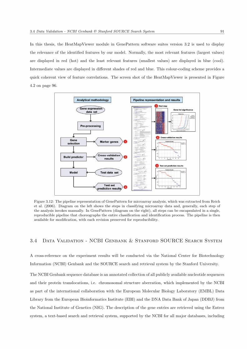
3.4 Data Validation - NCBI Genbank & Stanford SOURCE Search System 91
In this thesis, the HeatMapViewer module in GenePattern software suites version 3.2 is used to display
the relevance of the identified features by our model. Normally, the most relevant features (largest values)
are displayed in red (hot) and the least relevant features (smallest values) are displayed in blue (cool).
Intermediate values are displayed in different shades of red and blue. This colour-coding scheme provides a
quick coherent view of feature correlations. The screen shot of the HeatMapViewer is presented in Figure
4.2 on page 96.
Figure 3.12: The pipeline representation of GenePattern for microarray analysis, which was extracted from Reichet al. (2006). Diagram on the left shows the steps in classifying microarray data and, generally, each step ofthe analysis invokes manually. In GenePattern (diagram on the right), all steps can be encapsulated in a single,reproducible pipeline that choreographs the entire classification and identification process. The pipeline is thenavailable for modification, with each revision preserved for reproducibility.
3.4 Data Validation - NCBI Genbank & Stanford SOURCE Search System
A cross-reference on the experiment results will be conducted via the National Center for Biotechnology
Information (NCBI) Genbank and the SOURCE search and retrieval system by the Stanford University.
The NCBI Genbank sequence database is an annotated collection of all publicly available nucleotide sequences
and their protein translocations, i.e. chromosomal structure aberration, which implemented by the NCBI
as part of the international collaboration with the European Molecular Biology Laboratory (EMBL) Data
Library from the European Bioinformatics Institute (EBI) and the DNA Data Bank of Japan (DDBJ) from
the National Institute of Genetics (NIG). The description of the gene entries are retrieved using the Entrez
system, a text-based search and retrieval system, supported by the NCBI for all major databases, including

3.5 Summary 92
PubMed bibliography, taxonomy project, protein sequences and structures, and many others. In this thesis,
the Entrez Gene, one of the several search tools supported by the Entrez system is used to validate our gene
findings.
The SOURCE is a unification tool which dynamically collects and compiles data from various scientific
databases, such as Gene Ontology (GO), UniGene, SAGE, Genbank and PubMed. It is a text-based search
and retrieval system supported by the Stanford University that encapsulates the genetics and molecular
biology of genes from variety living organisms, i.e. homo sapiens (human), mus musculus (house mouse),
rattus norvegicus (domestic rat), into easy to navigate gene reports.
The screen shot for validating microarray gene expression profile using the NCBI Genbank and the SOURCE
system is presented in Figure 4.12 on page 114.
3.5 Summary
In this chapter, we discussed the design of our feature extraction model. We have shown technical perspec-
tives on both GAs and ANNs, how to use ANNs to calculate the fitness values of GA chromosomes. We
have applied simple mathematical formulas in fitness computation including the centroid vector principle
to calculate mean of each classes, the Euclidean distance to measure the proximity of samples from each
classes and network activation functions to determines the potential firing of a node. We have also applied a
genomic analysis platform, GenePattern software suite, to demonstrate the gene selection results graphically.
The NCBI Genbank and the SOURCE search system have been used to validate the gene findings obtained
by our model.
In Chapter 4, the prototype and the experimental study of our model will be presented.

Chapter 4
Prototype and Experimental Study
Chapter 3 presented the conceptual design of our feature extraction model to support the theme of this
thesis. This chapter demonstrates the prototype of our model, namely Genetic Algorithm-Neural Network
(GANN). The novelty of the GANN model is its simplicity that follows the Ockham’s Razor principle which
can minimise the potentiality of gene variability errors incurred by data preprocessing which is discussed
in Chapter 2. The construction of ANN for computing the fitness values of the chromosomes described
in the previous chapter will be explained. Since a standard GA technique, except the fitness computation
technique, has been used in the pattern evaluation module, we did not explain the GA construction steps in
details, however, we outlined the overview of the implementation for GA evaluation.
The objectives of this chapter are to describe the tools, the prototype and the experimental study for
supporting the theme of this thesis. This chapter contains six sections. Section 4.1 presents the software
tools used in this thesis, including the programming tool for developing the prototype and the synthetic data
sets, the data mining tool for validating the findings of the bioassay data sets and the visualisation tools to
present graphically the result findings and the data sets. Section 4.2 explains the needs for the transposition
process to preprocess microarray data. The GANN prototype is presented in Section 4.3 and Section 4.4
describes the validation steps conducted using the NCBI Genbank and the SOURCE search system. Section
4.5 describes the research methodology used to test the hypotheses of this thesis and finally, Section 4.6
concludes the chapter.
4.1 Tools used in the Prototype
Five tools: C++, WEKA, GenePattern, Microsoft Excel and R Project, are used to support the theme of
this thesis. C++ is an object-oriented programming language that is used for the coding of the GANN
93

4.1 Tools used in the Prototype 94
prototype. WEKA is a data mining software that is used to compute the statistical significance of the gene
findings and to validate the bioassay findings. GenePattern is a genomic analysis platform that is used
to visualise the correlation of the gene findings. Microsoft Office Excel is a spreadsheet software from the
Microsoft Office Package Suite that is used to graphically present the findings from the prototype. Lastly,
R Project is a language and environment that is used to visualise the data interactions.
4.1.1 Programming language for developing the prototype and the synthetic data
Although C programming language is more commonly used in the machine learning community, C++ is
chosen to be the language for developing the prototype since it is less complex in terms of coding commands
and rich in variety of built-in functions without a sophisticated programming environment. The screen
shots of the important functions in the prototype can be found in Appendix A. In addition to the GANN
prototype, two specially written C++ programs are coded to which one is used to transpose the microarray
experimental data sets and the other program is used to construct the synthetic data sets. All C++ coding
were programmed on the LINUX environment.
For the synthetic data program, the values of genes were designed based on a standard Gaussian distribution,
i.e. the mean value of 0 (µ = 0) and the standard deviation of 1 (δ = 1), with the exception on 30 randomly
selected genes, from each data set, which were created with different µ values. Table 4.1 presents the settings
in the synthetic data sets. In the synthetic data set 1, the 30 differentially expressed genes were created with
µ = 2.0 and were labelled with the gene indexes 1-15 and 5001-5015. In the synthetic data set 2, 10 out of
the 30 genes were created with µ = 0.5 (gene indexes 1-10) and the remaining 20 genes were created with
µ = 2.0 (gene indexes 11-30).
Table 4.1: The description of the synthetic data sets.
Data set Description Significant features
Synthetic data set 1 100 samples equally distributed into 2class. Each sample has 10000 featureswhich were standardised with µ = 0and δ = 1.
30 significant features, with thefeature indexes 1-15 and 5001-5015, were standardised withµ = 2.0 and δ = 1.
Synthetic data set 2 67 samples distributed into 3 classes,i.e. 20 samples in class 1, 30 in class2 and 17 in class 3. Each sample has5000 features which were standardisedwith µ = 0 and δ = 1.
30 significant features, with thefeature indexes 1-10 were stan-dardised with µ = 0.5 and δ =1 and the feature indexes 11-30were standardised with µ = 2.0and δ = 1.

4.1 Tools used in the Prototype 95
4.1.2 Tool for evaluating the significance of the findings
WEKA (Waikato Environment for Knowledge Analysis) is a data mining software developed by the University
of Waikato (Hall et al., 2009). It is a free software that is available to download from its original website
(WEKA data mining software). WEKA contains numerous collection of machine learning and data mining
tools, such as data preprocessing, classification, regression, clustering, association rules and visualisation.
Amongst these tools, the Information Gain (GainRatio) is selected to measure the significant of individual
genes extracted from the microarray and synthetic data sets. Four cost-sensitive classifiers, which are naive
bayes (NB), support vector machine (SMO), C4.5 tree (J48) and random forest (RF) are used to validate the
significance of the attributes extracted from the bioassay data sets. Additionally, the principal component
analysis (PCA) is used as a comparative tool in the bioassay data sets.
For GainRatio and PCA, the default parameter settings on the Attribute Selection tool were used. To
construct the cost-sensitive classifier, the Cost Sensitive parameter on the Meta option for NB, SMO and
RF, and the MetaCost parameter for J48 tree were selected. Figure 4.1 shows the screen shot to construct
a Cost-Sensitive NB classifier (CSC NB) on the WEKA environment. We used the default WEKA settings
for NB and RF classifiers. For SMO classifier, we set the build logistic models parameter to “true” and for
J48 tree, we amended the Unpruned tree parameter to “true”.
Figure 4.1: The screen shot for constructing a CSC NB on the WEKA environment.

4.1 Tools used in the Prototype 96
4.1.3 Tool for visualising the significance of the gene findings
GenePattern software suites is a freely available software package developed at the Broad Institute of MIT and
Harvard (Reich et al., 2006) that provides access to a broad array of computational methods used to analyse
genomic data via the Broad Institute website (GenePattern software suites). HeatMapViewer, one of the
GenePattern tools, which allows the transformation from the numeric findings into graphical representations
and provides a global view on the features interaction without any form of programming syntax, is used to
support the findings of the GANN prototype. The colour-coding scheme in the HeatMapViewer provides a
quick coherent view of feature correlations.
Figure 4.2 presents the screen shot to produce a heat-map on the GenePattern environment. In the HeatMap
Viewer module, the expression values are standardised with the mean value, ranging from -3 to 3, and the
standard deviation of 1. These values are presented in 2 different colour shades, i.e. red and blue. High
expression values are displayed in red indicating with positive values and the negative value representing low
expression values which is displayed in blue. Intermediate expression values are displayed in different shades
of red and blue. We used the default HeatMap Viewer settings to generate heat-maps for our findings on
microarray data.
Figure 4.2: The screen shot generating heat-map using HeatMap Viewer.
4.1.4 Tool for visualising the findings
Microsoft Office Excel is a spreadsheet application written and distributed by Microsoft. It is featured with
calculation functions, graphing tools, pivot tables and VBA macro programming language. In this thesis,
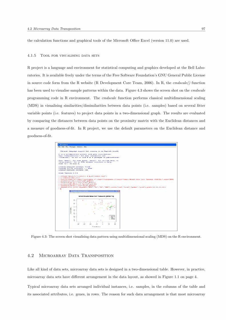
4.2 Microarray Data Transposition 97
the calculation functions and graphical tools of the Microsoft Office Excel (version 11.0) are used.
4.1.5 Tool for visualising data sets
R project is a language and environment for statistical computing and graphics developed at the Bell Labo-
ratories. It is available freely under the terms of the Free Software Foundation’s GNU General Public License
in source code form from the R website (R Development Core Team, 2006). In R, the cmdscale() function
has been used to visualise sample patterns within the data. Figure 4.3 shows the screen shot on the cmdscale
programming code in R environment. The cmdscale function performs classical multidimensional scaling
(MDS) in visualising similarities/dissimilarities between data points (i.e. samples) based on several fitter
variable points (i.e. features) to project data points in a two-dimensional graph. The results are evaluated
by comparing the distances between data points on the proximity matrix with the Euclidean distances and
a measure of goodness-of-fit. In R project, we use the default parameters on the Euclidean distance and
goodness-of-fit.
Figure 4.3: The screen shot visualising data pattern using multidimensional scaling (MDS) on the R environment.
4.2 Microarray Data Transposition
Like all kind of data sets, microarray data sets is designed in a two-dimensional table. However, in practice,
microarray data sets have different arrangement in the data layout, as showed in Figure 1.1 on page 4.
Typical microarray data sets arranged individual instances, i.e. samples, in the columns of the table and
its associated attributes, i.e. genes, in rows. The reason for such data arrangement is that most microarray
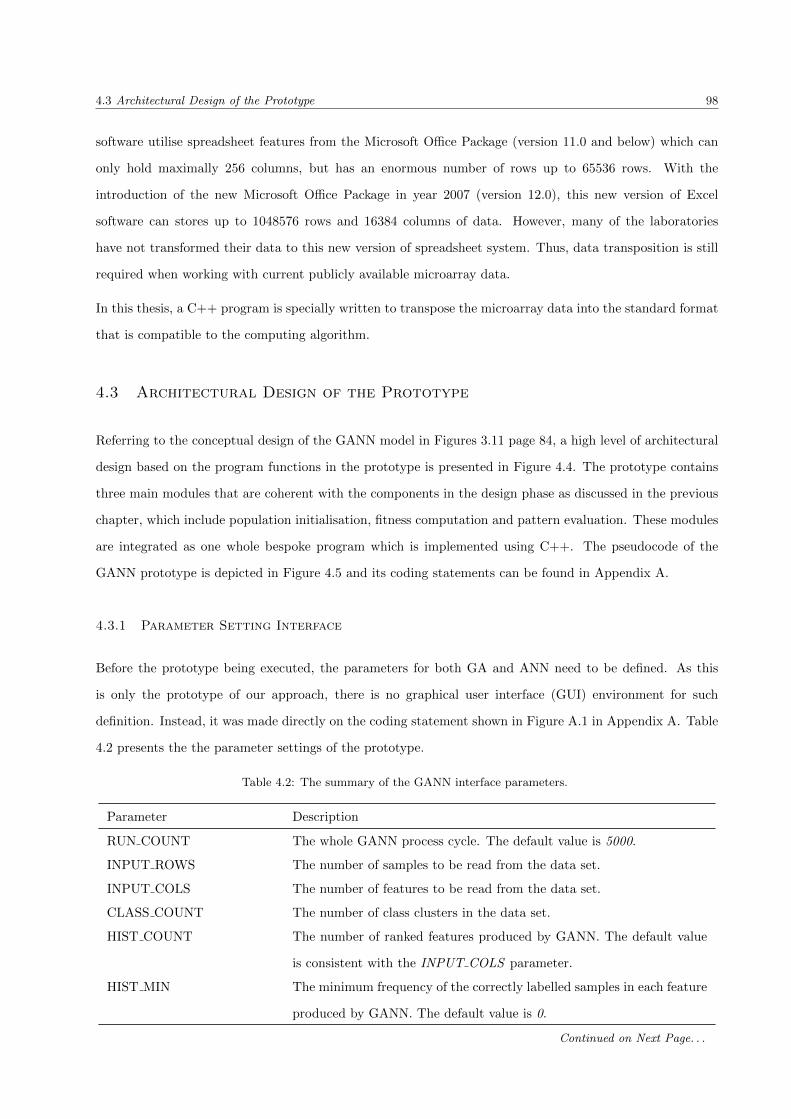
4.3 Architectural Design of the Prototype 98
software utilise spreadsheet features from the Microsoft Office Package (version 11.0 and below) which can
only hold maximally 256 columns, but has an enormous number of rows up to 65536 rows. With the
introduction of the new Microsoft Office Package in year 2007 (version 12.0), this new version of Excel
software can stores up to 1048576 rows and 16384 columns of data. However, many of the laboratories
have not transformed their data to this new version of spreadsheet system. Thus, data transposition is still
required when working with current publicly available microarray data.
In this thesis, a C++ program is specially written to transpose the microarray data into the standard format
that is compatible to the computing algorithm.
4.3 Architectural Design of the Prototype
Referring to the conceptual design of the GANN model in Figures 3.11 page 84, a high level of architectural
design based on the program functions in the prototype is presented in Figure 4.4. The prototype contains
three main modules that are coherent with the components in the design phase as discussed in the previous
chapter, which include population initialisation, fitness computation and pattern evaluation. These modules
are integrated as one whole bespoke program which is implemented using C++. The pseudocode of the
GANN prototype is depicted in Figure 4.5 and its coding statements can be found in Appendix A.
4.3.1 Parameter Setting Interface
Before the prototype being executed, the parameters for both GA and ANN need to be defined. As this
is only the prototype of our approach, there is no graphical user interface (GUI) environment for such
definition. Instead, it was made directly on the coding statement shown in Figure A.1 in Appendix A. Table
4.2 presents the the parameter settings of the prototype.
Table 4.2: The summary of the GANN interface parameters.
Parameter Description
RUN COUNT The whole GANN process cycle. The default value is 5000.
INPUT ROWS The number of samples to be read from the data set.
INPUT COLS The number of features to be read from the data set.
CLASS COUNT The number of class clusters in the data set.
HIST COUNT The number of ranked features produced by GANN. The default value
is consistent with the INPUT COLS parameter.
HIST MIN The minimum frequency of the correctly labelled samples in each feature
produced by GANN. The default value is 0.
Continued on Next Page. . .

4.3 Architectural Design of the Prototype 99
Table 4.2 – Continued
Parameter Description
HIST MAX The maximum frequency of the correctly labelled samples in each fea-
ture produced by GANN. The default value is consistent with the IN-
PUT ROWS parameter.
GA POPSIZE The population sizes to be examined {100, 200, 300}. User can input
integer values that is higher or lower than the defined sizes.
GA EVALS The evaluation sizes to be examined {5000, 10000, 15000, 20000, 25000,
30000, 35000, 40000, 45000, 50000}. User can input integer values that
is higher or lower than the defined sizes.
GA PRECISION The fitness confidence (accuracy) level of GANN. The default value is
consistent with the INPUT ROWS parameter.
GA MUTATIONDIST The mutation point (the point on the chromosome to be changed) of the
string (offspring). The default value is 0.5.
GA MUTATIONRATE The mutation rate. The default value is 0.1.
GA XFACTOR The cut-point on the parent strings. The default value is 2 (single-point
crossover).
GA CROSSOVER The execution of crossover function. The default setting is true. User
can de-activates this function by amending the parameter to false.
GA TOURNAMENTSIZE The size of the tournament selection. The default value is 2.
MLP ISIZE The input nodes in the input layer. The default value is 10.
MLP HSIZE The hidden nodes in the hidden layer. The default value is 5.
MLP OSIZE The output nodes in the output layer. The value must consistent with
the CLASS COUNT parameter.
MLP ACT The activation function. The available functions include binary sigmoid,
linear, tanh, threshold.
MLP SIZE The network weights including the bias nodes. User can amend the
number of bias nodes in the hidden and output layers.
Three data set parameters, which are INPUT ROWS, INPUT COLS and CLASS COUNT ; were used to
describe the experimental data set. The INPUT ROWS is the total number of samples in the data set, the
INPUT COLS is the total number of features in the data set and the CLASS COUNT is the number of
classes in the data set.
The layout of the results is defined by three parameters, i.e. HIST COUNT, HIST MIN and HIST MAX.
The HIST COUNT indicates the total number of ranked features to be displayed by the prototype, the
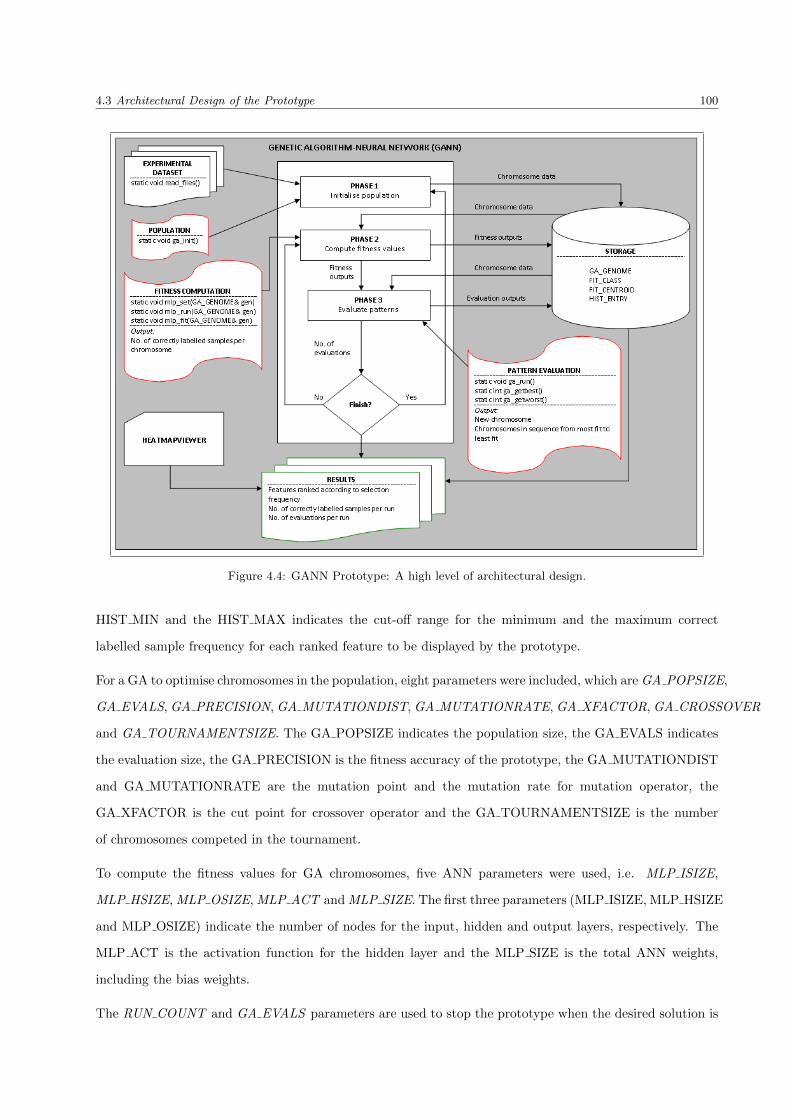
4.3 Architectural Design of the Prototype 100
Figure 4.4: GANN Prototype: A high level of architectural design.
HIST MIN and the HIST MAX indicates the cut-off range for the minimum and the maximum correct
labelled sample frequency for each ranked feature to be displayed by the prototype.
For a GA to optimise chromosomes in the population, eight parameters were included, which are GA POPSIZE,
GA EVALS, GA PRECISION, GA MUTATIONDIST, GA MUTATIONRATE, GA XFACTOR, GA CROSSOVER
and GA TOURNAMENTSIZE. The GA POPSIZE indicates the population size, the GA EVALS indicates
the evaluation size, the GA PRECISION is the fitness accuracy of the prototype, the GA MUTATIONDIST
and GA MUTATIONRATE are the mutation point and the mutation rate for mutation operator, the
GA XFACTOR is the cut point for crossover operator and the GA TOURNAMENTSIZE is the number
of chromosomes competed in the tournament.
To compute the fitness values for GA chromosomes, five ANN parameters were used, i.e. MLP ISIZE,
MLP HSIZE, MLP OSIZE, MLP ACT and MLP SIZE. The first three parameters (MLP ISIZE, MLP HSIZE
and MLP OSIZE) indicate the number of nodes for the input, hidden and output layers, respectively. The
MLP ACT is the activation function for the hidden layer and the MLP SIZE is the total ANN weights,
including the bias weights.
The RUN COUNT and GA EVALS parameters are used to stop the prototype when the desired solution is

4.3 Architectural Design of the Prototype 101
INITIALISE GANN parameters
REPEAT until termination criteria A (Max. no. of iteration) is satisfied {
Generate GA population
Calculate fitness values for each string in the population {
DO WHILE EOF {
a. Generate network weights
b. RUN ANN
c. Compute centroid values for each class using target output
d. Calculate distance between samples and classes
e. Label samples to its nearest class
}
}
REPEAT until termination criteria B (Max. no. of fitness evaluation ||
predefined precision value) is satisfied {
Select 2 strings as parents for reproduction
Perform GA operators {
For network evolution {
a. Crossover 2 set of network weights to produce new set of network weights
b. Mutate the new set of weights
}
For feature evolution {
a. Crossover 2 strings to produce new set of string
b. Mutate the new string
}
}
Calculate fitness value for new string
Replace the least fit string with the new string
}
Calculate the number of correctly labelled samples
}
PRODUCE summary results
Figure 4.5: The pseudocode of the GANN prototype.
achieved (GA PRECISION ). The RUN COUNT parameter performs external looping on the entire extrac-
tion process and the GA EVALS parameter internally repeating the fitness computation module.
4.3.2 Population Initialisation Phase
In this module, two program functions are executed, which are the read files() and ga init() functions. Figure
4.6 presents the module’s flowchart.
This module begins when the data set is retrieved by the prototype. The read files function reads the entire
data set and stores the data in a two-dimensional input matrix with rows indicate samples and columns
indicate features. This input matrix is ready for use by the subsequent functions. After the input matrix
was created, subsets of the features from the matrix is extracted using the ga init function. The number of
extracted features is reliant on the population size and the chromosome size. For example, in the population
4.3 Architectural Design of the Prototype 102
size of 300 and the chromosome size of 10, the ga init function will extract 3000 features (300 x 10) from
the input matrix. The extracted feature subset is stored in the GA GENOME array for later use. The
subsequent program functions will process the feature subsets in the array, rather than the features in the
input matrix. The configuration statement for the GA GENOME array and the coding statement for the
ga init function are presented in Figures A.2 and A.4a in Appendix A, respectively.
Figure 4.6: Population Initialisation Phase: The system flowchart.
It is important to note that, other than the data transposition for microarray data, there is no data pre-
processing steps, such as pre-filtering, imputation techniques and normalisation methods, are applied to the
experimental data sets, as is in the traditional way for analysing microarray data. The reason for excluding
such traditions is that we would like to avoid any of the sort of errors that may induced by these preprocessing
steps.
4.3.3 Fitness Computation Phase
After the feature subsets are loaded in the GA GENOME array, a 3-layered feedforward ANN with the
structure of 10-5-O is constructed to calculate the fitness values for each feature subset in the array. Three
program functions are created in this module are the mlp set(), mlp run() and mlp fit() functions. The overall
system flowchart of this module is presented in Figure 4.7 and the coding statements of these functions can

4.3 Architectural Design of the Prototype 103
be found in Figure A.3 in Appendix A.
Figure 4.7: Fitness Computation Phase: A high level system flowchart.
In this module, the mlp set function is first executed to initialise the network weights for each network layer
and the bias values for the hidden and output layers. The initial weight values are randomly selected from
the range of [0,1]. The mlp set function then reads the input nodes from the GA GENOME array. In other
words, 10 features will be used as the input nodes in the ANN when the chromosome size is set to 10. The
mlp run function is then executed to process each sample of the data set for which the network must be run
and calculates activation outputs, which is then used by the mlp fit function to calculate the fitness of the
feature subset. The fitness output of the mlp fit function is stored in the GA GENOME array.

4.3 Architectural Design of the Prototype 104
4.3.3.1 mlp set() function
The mlp set() function is the looping function based on the for loop command, used to construct the network
model based on the network size defined in the parameter setting interface module.
4.3.3.2 mlp run() function
After the network is constructed, the mlp run() function processes samples for each chromosome in the
GA GENOME array. Once the input activations of the network are set, using the activation value and the
element values, the network can be run in sequential order. This process is often called “feedforward” in the
context of ANN.
In the mlp run function, as shown in Figure 4.8, the first input weight for the first input node is read from
the GA GENOME array to compute the activation value for the input node f(Ainput). The network is
then process the second input weight for the second input node. This process is repeated until all the input
nodes have assigned activation values. In the input layer, the identity activation function (f(x) = Σxi) is
used to calculate input activation values.
The network then process the nodes in the hidden layer by reading the first hidden weight and its bias from
the GA GENOME array to calculate its hidden activation value f(Ahidden). In the hidden layer, each
hidden node is supported by a bias node B, meaning that 5 bias nodes will be generated by the network for
5 hidden nodes. This process is iterated until all the hidden nodes have assigned activation values. In the
hidden layer, four commonly used activation functions f(x), i.e. sigmoid, linear, hyperbolic tangent (tanh)
and threshold functions are examined in this thesis. The equations for these activation functions can be
found in Figure 3.10 on page 81. The hidden activation function can be expressed as f(x) = Σxij + Bj , in
which f(x) is the selected activation function, xij is the weight for the input node to hidden node, and Bj
are the bias weights for the hidden nodes.
Based on the outputs from the hidden layer, the network calculates the activation value f(Aoutput) for
each output node in the output layer. A two dimensional matrix A, as shown in Expression 4.1, that holds
the activation values from the output layer is produced and this matrix is used by the mlp fit function to
calculate the fitness value for each feature subset in the GA GENOME array.
A =
a1s1 a2s1 . . . aks1
a1s2 a2s2 . . . aks2...
......
...
a1sn a2sn . . . aksn
, (4.1)
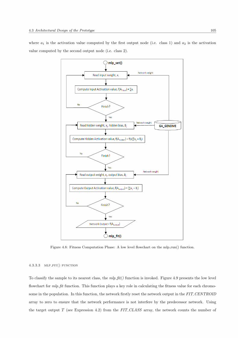
4.3 Architectural Design of the Prototype 105
where a1 is the activation value computed by the first output node (i.e. class 1) and a2 is the activation
value computed by the second output node (i.e. class 2).
Figure 4.8: Fitness Computation Phase: A low level flowchart on the mlp run() function.
4.3.3.3 mlp fit() function
To classify the sample to its nearest class, the mlp fit() function is invoked. Figure 4.9 presents the low level
flowchart for mlp fit function. This function plays a key role in calculating the fitness value for each chromo-
some in the population. In this function, the network firstly reset the network output in the FIT CENTROID
array to zero to ensure that the network performance is not interfere by the predecessor network. Using
the target output T (see Expression 4.2) from the FIT CLASS array, the network counts the number of

4.3 Architectural Design of the Prototype 106
samples in each class and these values are used to calculate the centroid value for each class Ck using the
activation results from the mlp run function (see Expression 4.1). The centroid values are stored in the
FIT CENTROID array, which will be used for labelling samples to its nearest class. The configuration
statements of the FIT CENTROID and FIT CLASS arrays can be found in Figure A.2 in Appendix A.
T =
ts1
ts2...
tsn
, (4.2)
where tsn is the target (actual) output for sample n in the data set.
When the centroid of the classes in the data set is calculated, the network computes the sample distance
for each class. In the distance proximity measure, the square root for the subtraction of output activation
value for each sample to each class centroid is calculated (√
(Aik − Cik2) and the results are stored in the
FIT CLASS array, which is used to label the sample to the nearest class. Expression 4.3 presents a two-
dimensional matrix used in the FIT CLASS array to store the proximity values of samples to each class
centroid.
O =
o1s1 o2s1 . . . oks1
o1s2 o2s2 . . . oks2...
......
...
o1sn o2sn . . . oksn
, (4.3)
where oksn is the network output for sample n for class centroid k.
Based on the proximity values in the matrix O, the network compares values of both the centroid and the
sample and labelled sample to the class with the smallest discrepancy value. Thus, the matrix O in the
FIT CLASS array is updated as:
∆O =
o1s1 o2s1 . . . oks1 class 1
o1s2 o2s2 . . . oks2 class 2...
......
...
o1sn o2sn . . . oksn class k
. (4.4)
The matrix ∆O is the actual output generated by the network. To count the number of correctly labelled
samples for each chromosome, the network output is compared to the target output. For each correctly
labelled sample, a constant value of 1 is added to the chromosome’s fitness score, which is saved in the
GA GENOME array.
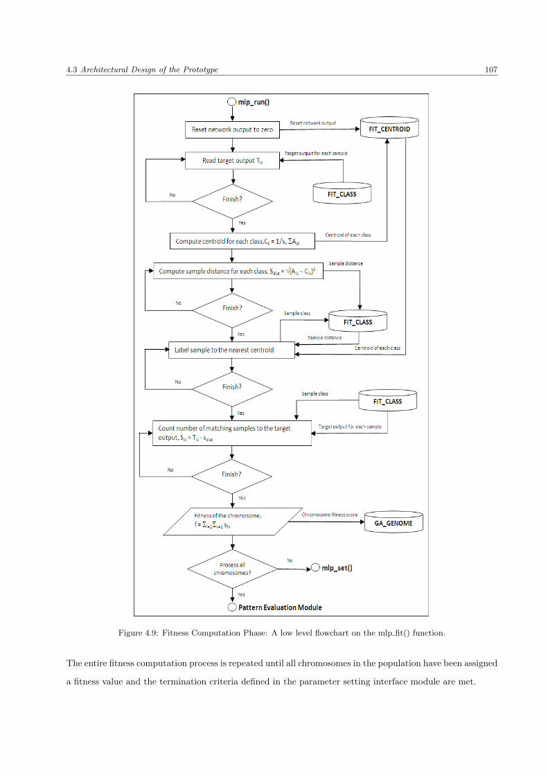
4.3 Architectural Design of the Prototype 107
Figure 4.9: Fitness Computation Phase: A low level flowchart on the mlp fit() function.
The entire fitness computation process is repeated until all chromosomes in the population have been assigned
a fitness value and the termination criteria defined in the parameter setting interface module are met.

4.3 Architectural Design of the Prototype 108
4.3.4 Pattern Evaluation Phase
When all chromosomes have been assigned fitness values, the evaluation process begins by first identifying a
pair of chromosome from the GA GENOME array for producing new offspring. The ga run() function is used
to execute such process and the ANN process (fitness computation module) is evoked to compute the fitness
value for this offspring. The GA compares all chromosomes in the array to identify the least fit chromosome,
which is then replaced by the new chromosome; and sorts these chromosomes in sequential order, ranking
from the best fit chromosome to the least fit chromosome. The comparison process is performed using
the ga getworst() function and the sorting process is invoked by the ga getbest() function. The latter two
functions are invoked in the ga run function. In other words, the ga getworst and ga getbest functions are
the subfunctions executed by the ga run function. Figure 4.10 presents the system flowchart of the module
and the coding statements for this module can be found in Figure A.4 in Appendix A.
4.3.4.1 ga run() function
The ga run() function plays a key role in evolving chromosomes and it, in fact, represents the entire GA
evolution process and to stop the prototype from over-learnt. In the ga run function (see Figure 4.10a),
the GA randomly selects a chromosome from the GA GENOME array for comparison. The GA is then
selects another chromosome from the array and the fitnesses of these two chromosomes are compared. The
chromosome with high fitness value is chosen as the parent chromosome a. Such comparison process is known
as tournament selection in GA. Similar process is performed to find the parent chromosome b. When the
GA has identified parent chromosomes, these chromosomes are cross-overed to produce new offspring. This
is known as reproduction in the context of GA.
In this module, two types of reproduction process are performed. They are network weight optimisation
process and conventional GA process (i.e. feature subset optimisation). For the network weight optimisation
process, the weight of the first input node from both parent are cross-overed based on the random crossover
point (i.e. cut point) in the range of [1, network size - 2], to obtain the new input weight for the first input
node in the new network. This new weight is then mutated with the Gaussian range [0, 0.5] and the mutated
weight is saved in the GA GENOME array. The process is repeated until weights for all nodes in both parent
are optimised. The similar optimisation process is used to optimise feature subset in the new offspring. For
feature subset optimisation, the crossover point of the features is selected randomly in the range of [1, Input
nodes - 2] and the mutation point is selected randomly in-between the range [-z, +z], in which the z value is
the division of the entire features in the data set over 100. In other words, for the data set containing 7000
features using the network structure 10-5-2, the crossover point for new network is [1, 65], the crossover and
mutation points for new feature subset is [1, 8] and [-70, 70], respectively.

4.3 Architectural Design of the Prototype 109
(a) The ga run() function.
Figure 4.10: Pattern Evaluation Phase: A low level flowchart on ga run() function.
The fitness of this new offspring is calculated by repeating the processes in the fitness computation module
and the comparison between chromosomes is carried out by the ga getworst function and the feature ranking
is performed by the ga getbest(). The processing step in these two functions is presented in Figure 4.10b.
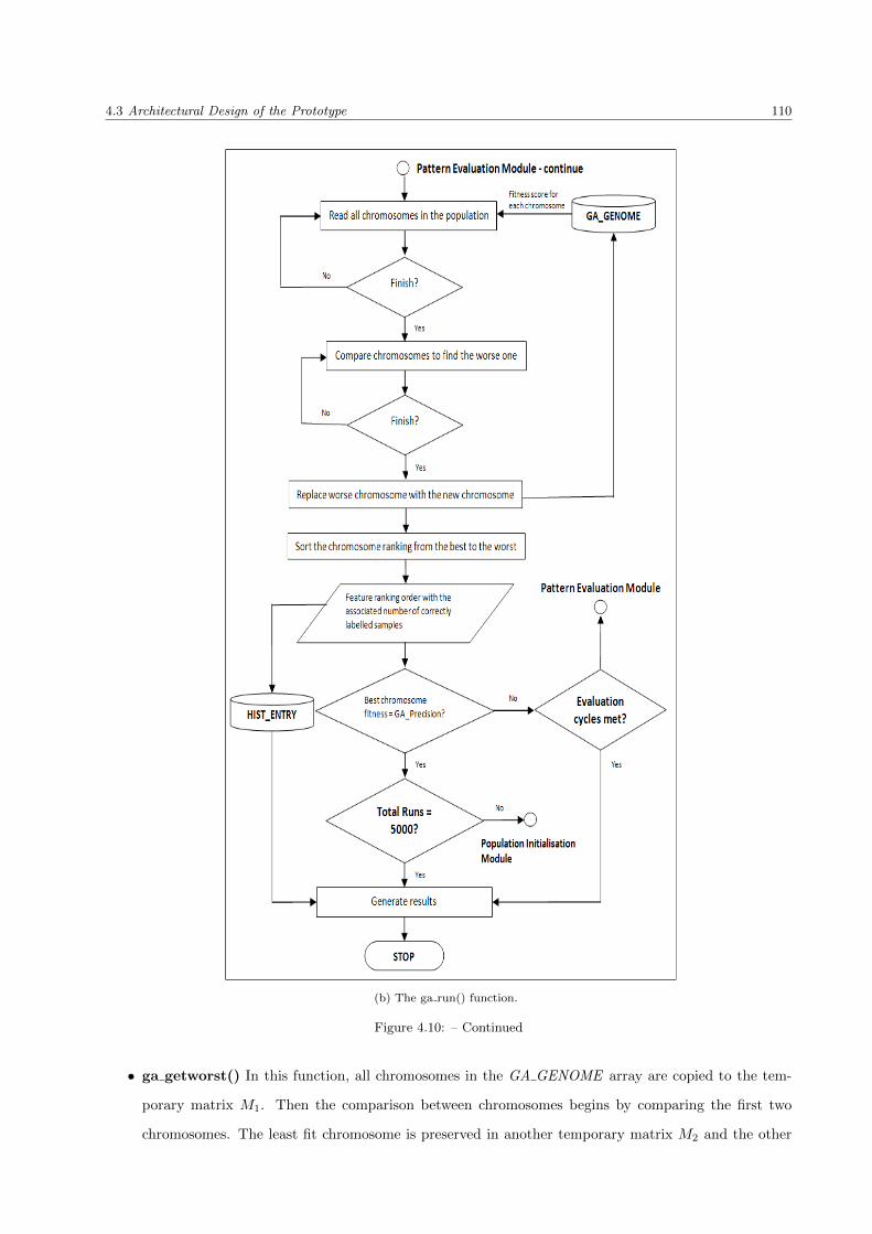
4.3 Architectural Design of the Prototype 110
(b) The ga run() function.
Figure 4.10: – Continued
• ga getworst() In this function, all chromosomes in the GA GENOME array are copied to the tem-
porary matrix M1. Then the comparison between chromosomes begins by comparing the first two
chromosomes. The least fit chromosome is preserved in another temporary matrix M2 and the other

4.4 Data Validation - NCBI Genbank & Stanford SOURCE Search System 111
chromosome is removed from the matrix M1. The second chromosome from the matrix M1 is retrieved
and compared with the chromosome in the matrix M2. The process is repeated until there are no
chromosome left in the matrix M1. The chromosome in the matrix M2 is considered as the worst
chromosome in the population and this chromosome is removed from the GA GENOME array. The
new offspring is replaced the position of the removed chromosome in the array. The contents of the
matrices M1 and M2 are emptied so that these matrices can be reused by other functions.
• ga getbest() When the new offspring is introduced to the GA GENOME array, the ga getbest function
is invoked by the ga run function. In this function, all chromosomes in the GA GENOME array are
copied to the temporary matrix M1. A chromosome y, randomly selected from the matrix M1, is
copied into the first pointer (i.e. fittest) in the temporary matrix M2 for comparison. The second
chromosome retrieved from the matrix M1 is compared with the chromosome y in the matrix M2. If
this chromosome has higher fitness score than the chromosome y, the chromosome y is moved one step
below the first pointer in the matrix and this new chromosome is allocated in the first pointer. If this
chromosome has lower fitness score than the chromosome y, this chromosome is added at the second
pointer after the chromosome y. This sorting process is repeated until there are no chromosome left
in the matrix M1 and the ranking of each feature in the chromosomes are stored in the HIST ENTRY
array.
4.3.5 Terminating the Prototype
Before the prototype stops running, the fitness score of the best chromosome is compared to the defined value
in the GA PRECISION parameter in the parameter setting interface module. If the fitness score matches
the value in the GA PRECISION parameter, the termination criteria based on the external iterating on the
entire GANN process is performed (RUN COUNT parameter). Otherwise, the termination criteria based
on the internal looping on the fitness computation process is invoked (GA EVALS parameter). For either
criteria, a summary result is produced when the prototype stops. This result comprising features ranking
based on their selection frequency in different classification accuracy, retrieved from the HIST ENTRY array.
The screen shot of the summary result processed by the HIST ENTRY array is presented in Figure 4.11
and the configuration of the HIST ENTRY array can be found in Figure A.2 in Appendix A.
4.4 Data Validation - NCBI Genbank & Stanford SOURCE Search System
Due to the rapid development of microarray annotations, most of the gene description, in both microarray
experimental data sets, was not supported by the NCBI Genbank nor can it be found in the Stanford

4.4 Data Validation - NCBI Genbank & Stanford SOURCE Search System 112
Figure 4.11: The screen shot of the HIST ENTRY array. Column 1 indicates the indexes of the features in thedata set; column 2 represents the total number of frequency selections for each index; column 3 represents thenumber of times the index has been selected with no mislabelled samples; column 4 shows the number of timesthe index has been selected with 1 mislabelled sample; and so on.
SOURCE search and retrieval system. Thus, great care is taken in validating the gene findings. Firstly, a
list of the unique gene number, i.e. Affymetrix Accession Number for the ALL/AML genes and Clone Image
Id for the SRBCTs genes, of the selected genes is uploaded into the SOURCE system. A variety of options
on the type of gene information can be selected in the system. Then, the outcome of the SOURCE system
is cross-referenced against the NCBI Genbank via the NCBI Entrez Gene system.
There are two main reasons for choosing the SOURCE system as one of the validation mechanisms in this
thesis. Firstly, it is far more user friendliness than the NCBI Genbank and it can process multiple gene
queries at the same time. Secondly, which is arguably the most important, that is, the SOURCE system can
process Clone Id of the cDNA gene, whereas the NCBI Genbank is unable to recognise the Clone Id of the
cDNA data.
To validate the gene findings of the GANN prototype, the following steps are performed:
1. A text-based document containing only the unique gene numbers of the selected genes, i.e. Accession
Number of the ALL/AML genes and Image Id (clone id) of the SRBCTs genes, was produced.
2. The document is then uploaded to the SOURCE system (Stanford SOURCE search and retrieval

4.5 Experimental Study 113
system) and the gene options: Gene Id, Gene Symbol and Gene Cytoband, are selected. When there
is more than one possible outcome of a specific gene found in the system, no result will be produced
for that gene. Most of the SRBCTs genes containing more than one possible result in the SOURCE
system. This is mainly due to different cDNA protocol and annotation being used in different research
laboratories.
3. The annotation results obtained by the SOURCE system was then compared with the annotations used
in the experimental data sets. For the SRBCTs findings, an additional comparison on the annotation
results in the SOURCE system and the up-to-date gene annotations from the original authors was
performed. This is to prevent any incorrect annotation being used in our findings.
4. For gene annotations that are not supported by the SOURCE system, the annotation of these genes is
entered individually into the NCBI Entrez Gene system (NCBI Genbank).
(a) For ALL/AML findings, the accession number of the gene is used to perform the search. When
more than one possible outcome is found in the Genbank, the annotation based on the term
“Homo Sapiens” is used. In the case where the accession number is invalid, the gene description
is used to perform the search in the system.
(b) For SRBCTs findings, the gene description of the gene is used to perform the search. Even so,
there is always some undefinable genes in the SRBCTs data set due to a generic description being
used in the data.
5. A complete list of genes containing the original unique gene number, the gene id and the cytoband of
the gene, was produced.
Figure 4.12 presents the steps for validating identified genes on the microarray data set.
4.5 Experimental Study
To support the theme of this research, a research methodology is applied on this thesis. There are several
research methodologies in computer science, such as simulation, mathematical proof and experimental study.
Our research uses the experimental study to test the hypotheses related to conceptual design and to system
performance. We validate our solution by comparing the results from the prototype with the expected results
from the synthetic data sets, the findings from the NCBI Genbank and the SOURCE search system, as well
as the results reported in the original studies.

4.5 Experimental Study 114
Figure 4.12: The steps for validating identified genes on the microarray data set. [1] A text-based documentcontaining the clone id or accession number of the selected genes is uploaded to the SOURCE entry and retrievalsystem. Options such as Gene Id, Gene Symbol and Gene Cytoband in the SOURCE system are selected. [2]The SOURCE system processed the clone id and [3] a text-based document containing the defined options isdisplayed. When there is more than one possible outcome on a specific clone id, the system indicated the words“Data not found” or “Multiple clusters” in the output result. [4] The results was then compared with the genedescriptions in the data set to ensure the correct result is obtained for each identified gene. [5] The annotationfor the gene with more than one possible outcome on the SOURCE system is entered into the NCBI genbankfor validation. The annotation based on the term “Homo Sapiens” is used for cross-referencing our findings.
4.5.1 Objectives of experimental study
Reference is made to the hypotheses of this research as stated in Section 1.4 on page 12, emphasising the
model simplicity, the model generalisability and the normalisation-free model, as well as the formation of
biologically relevant results. To test the hypotheses, our experimental study measures the performance of
four ANN activation functions: sigmoid (binary sigmoid), linear, tanh and threshold, for which each function
is represented by a separate system in the prototype. This is to indicate which activation function has the
best or worst performance when they are used to compute the fitness values of features in the same data

4.5 Experimental Study 115
sets with similar parameter settings applied. Thus, the experimental study serves five purposes as follows:
The first purpose is to assess the overall performance of each system to handle raw, unprocessed microarray
data sets. The term ‘raw’ used in this section refers to the original microarray data set, obtained from
the respective repository, with no preprocessing steps performed on data values. In this experiment, the
oligonucleotide microarray data set having large range between the maximum and the minimum values
within a gene in the data set is examined.
The second purpose of the study is to assess the overall performance of each system to handle different types
of microarray platforms. In this experiment, two microarray data sets with different array platforms and a
different number of classes are examined.
The third purpose of the study is to assess the implication of two main GA features: population size and the
number of fitness evaluations for analysing microarray data. This objective is to examine which population
size is best for data with high feature dimensions and the minimal number of evaluations required for
consistent results.
The fourth purpose of the study is to assess the generalisability of the prototype to select the most significant
attributes from a large, imbalanced data set that contains multiple data representation. In this experiment,
two bioassay data sets with different percentage of minority class (different number of active compounds)
are examined.
The last purpose of the experimental study is arguably the most important, that is, to check the accuracy
(correctness) of the work described here in extracting the desired features from the data sets. The accuracy
of the results is checked by comparing the results obtained via the prototype and our expected results in
synthetic data sets.
4.5.2 Experimental Data Sets
Six experimental data sets were used in the experimental study. These data sets comprise of microarray
data sets (i.e. ALL/AML and SRBCTs), synthetic data sets (i.e. synthetic data set 1 and synthetic data
set 2) and bioassay data sets (i.e. AID362 and AID688). The description of these data sets is presented in
Section 3.1 on page 58.
4.5.3 Experiment Design
The experiments are designed according to the objectives of the experimental study, which has been men-
tioned in Section 4.5.1 and the hypotheses of this thesis, is as follows:

4.5 Experimental Study 116
1. Varying sizes of data sets with varying numbers of samples allocated in each class cluster were used in
the experiments. We performed trial experiments on several different sizes of data and it was found
that data that had a class size between 2 to 3 and a ratio between samples and features is 1:100 showing
a significant performance difference between the systems. Thus, the experiments were conducted based
on the synthetic data with sample size varying from 67 to 100, feature size varying from 5000 to 10000
and class size varying from 2 to 3. Similar sets of experiments were also performed on the real-world
microarray data sets which have a sample size varying from 72 to 83, feature size varying from 2308 to
7129 and class size varying from 2 to 4. This design serves the first two purposes of the experimental
study.
2. Varying sizes of population and fitness evaluation on the GA were tested in the experiments. In the
GANN prototype, the values of GA parameters, i.e. the population size, the fitness evaluations size,
the crossover factor and the mutation rate, can be changed (see GANN interface in Figure A.1 in
Appendix A). Trial experiments were conducted on these parameters and it was found that there was
a minor influence of the mutation operator to the stability performance of the system, with mutation
rate varying from 0.1 to 0.5. When the mutation rate more than 0.5 was applied, the system became
unstable and different set of genes were produced in the repeated trial when similar set of parameters
were used. This could be a precursor to the over-fitting problem. Therefore, we retained a small
mutation rate, i.e. 0.1, in all systems.
We also conducted trial experiments based on the population size varying from 100 to 700 and the
fitness evaluation size varying from 1000 to 50000. The trial results showed that convergence began
in most systems when the population size reached 300 and the fitness evaluation size 20000. However,
there was not much difference in system performance for population size, ranging from 300 to 700.
Therefore, the experiment was conducted on a population size varying from 100, 200 and 300. We
performed the experiments on smaller fitness evaluation sizes, started from 5000 and each time, the
evaluation was increased another 5000 cycles, until the maximum evaluation size of 50000 is reached.
This design supports the third purpose of the experimental study.
3. Varying levels of fitness precision in the prototype were examined in the experiment. The default values
of the precision parameter is usually consistent with the sample size, i.e. 100% fitness precision score.
This value can be altered to different precision accuracies. The experiments based on three precision
levels varying from 95% to 100% were tested. This design argues our statement in Section 1.2.4 on
page 9 and supports the objectives of our research theme stated in Section 1.4 on page 12.
4. The comparison study based on the normalised and the raw microarray data set was performed to
support our argument concerning the implication of data normalisation process addressed in Section

4.6 Summary 117
1.2.2 on page 8. The experiments based on the ALL/AML microarray data set was conducted.
5. The experiments based on two bioassay data sets with the tanh-based GANN system were performed.
This design supports the fourth purpose of the experimental study.
All the above experiments were designed for the last purpose of the experimental study. The first and the
second experiments were assessed based on the number of significant genes extracted by the system, the
fitness accuracy of the system on the extracted genes and the processing time of the system. The integrity of
the findings was evaluated based on the comparison studies conducted in previous work and from a molecular
perspective.
4.6 Summary
In this chapter, we have discussed the tools used to support the theme of this thesis and explained the
prototype of the method outlined in Chapter 3. An experimental study were conducted to evaluate the
performance of the prototype from several aspects, including the effect of different precision levels, the
population sizes, the fitness evaluation sizes and different activation functions.
With the vast development of microarrays, and there are many ‘grey areas’ that need to be further investi-
gated, the existing feature selection models are unable to handle these areas. Questions, such as ‘which genes
trigger the development of specific cancer diseases?’ and ‘which genes shown the first sign of the recurrence
of mutated cells?’, are yet to be answered. These questions have been taken into consideration when we
constructed the prototype which aims to provide an insight into the elementary genes and triggered genes
in malignancy development. A fitness precision accuracy parameter is also built into the prototype, which
allow users to closely monitor the pattern of the disease development from the beginning stage to the final
stage.
In the next chapter, we carried out a comparative study of our results with the studies reported previously
and show how the hybridisation of GAs and ANNs is suitable for analysing microarray data as well as the
bioassay data.

Chapter 5
Experimental Results and Discussion
The prototype and the experimental study have been explained in the previous chapter. The objectives of
this chapter is to present the findings of the prototype including discussions of the experimental results. Four
GANN systems represent different activation functions, based on three population sizes and ten evaluation
sizes which were compared in this chapter.
The relevant graphs and tables to support the objectives of the experimental study and the hypotheses of
this thesis were produced in this chapter. Additional information on these graphs and tables can be found
in Appendix B.
5.1 System performance with different data sets in different population
sizes
In this section, we assess the overall system performance based on the synthetic data sets and the microarray
data sets. Three figures, each representing an evaluation criteria, were produced. Each figure presents a high
level view of system performance in terms of the the average number of the extracted genes in Figure 5.1,
the average fitness accuracy of the extracted genes in Figure 5.2 and the average elapsed time (processing
time) in Figure 5.3, based on three population sizes, ranging from 100, 200 to 300. The complete list of the
extracted gene by each system in the four data sets are presented in Appendix B.
The four systems shown in the figures represent four different ANN activation functions used in the GANN
prototype to compute the fitness values for each subset of genes in the population. These systems comprise
of sigmoid, linear, tanh and threshold based.
118

5.1 System performance with different data sets in different population sizes 119
5.1.1 The number of significant genes
With observation on the synthetic data sets in Figure 5.1, all systems have extracted an almost similar
number of predefined genes in the synthetic data set 1 and in every population size. The linear based system
has the highest number of predefined genes found in both synthetic data sets, i.e. on average 30 and 16 with
the population size 300 in the synthetic data set 1 and the synthetic data set 2, respectively. The tanh based
system has the lowest number of predefined genes found in the synthetic data set 2, i.e. on average 11 out
of 30 genes in the population size 300.
Figure 5.1: The average number of significant genes extracted by each system based on the selection frequencyof 50 and above. The linear based system has the highest number of extracted genes in both synthetic datasets and the ALL/AML data set, while the other three systems have a similar performance in these data sets.None of the systems has a significant performance in the SRBCTs data set. In order words, all systems have acomparative performance in the SRBCTs data set.
For microarray data sets, there is a significant difference in the number of genes extracted by the linear based
system and the other three systems in the ALL/AML data set. The linear based system has found more
genes in every population size, while the other three systems have an almost equal number of genes was
found in every population size. For SRBCTs data set, a significant fluctuation on the number of extracted
genes by each system in every population size. In the population size 100, the sigmoid based system has
the highest number of genes found, while the linear based system has the lowest number of genes found
when a similar parameter was applied. When the population size is increased to 200, the threshold based
system has found a slightly higher number of genes than the sigmoid based system, while the tanh based
system showed a significantly decreased number of genes was found. A similar observation was made on
the decreased number of extracted genes by the sigmoid and tanh based systems in a population size 300.
When a similar population size was applied to the linear and the threshold based systems, both systems had

5.1 System performance with different data sets in different population sizes 120
a higher number of genes extracted than the sigmoid and tanh based systems.
An interesting phenomenon was observed on the number of genes extracted on the data sets when the
population size is increased. There are, on average, 11.47% (i.e. 11.64% on sigmoid based, 9.12% on linear
based, 11.74% on tanh based and 13.39% on threshold based) and 14.76% (i.e. 18.89% on sigmoid based,
9.16% on linear based, 17.42% on tanh based and 13.57% on threshold based) of decreased number of
significant genes extracted by all systems on ALL/AML and SRBCTs data sets, respectively. Conversely, a
significant increased number of predefined genes (on average 55.05% on synthetic data set 2) by each system
on both the synthetic data sets. This is due to the quality (characteristics) of the data sets. Both the
synthetic data sets were generated based on different mean µ values in the Gaussian distribution; as a result,
there are no extreme maximum and minimum values in the genes and outliers, which most microarray data
suffer. Microarray data sets contain large value interval within a gene, especially the ALL/AML data set
that contains large number of suppressed genes expression (i.e. negative values). With the increase in the
population size, more chromosomes were exploited by the systems and consequently, more learning patterns
(i.e. chromosomes) have been presented to the systems to model a set of general rules from these patterns.
As indicated in Figure 5.1, all systems might under-learnt the rules in population size 100 due to insufficient
learning patterns to model these rules. With the increase population size to 200, the systems started to
explore more learning patterns, however, the rules were still imperfect in some way as microarray data sets
are highly imbalanced on the scale of available samples and the number of associated genes per sample, and
a high ratio of significant genes and noisy genes in the data sets. When the population size was increased to
300, the systems have been provided with sufficient learning patterns to model a set of better general rules
with lesser number of but most significant genes in the data sets. We will discuss the significance of the
extracted genes in Sections 5.3-5.4.
5.1.2 The fitness performance
With assessment on the fitness performance of each system in Figure 5.2 for synthetic data sets, there is
no significant difference between the systems’ performance in the synthetic data set 1 when the population
size are 200 and 300. This is because all the 30 predefined genes in the data set have been identified by all
systems, as is indicated in Figure 5.1 on page 119. Tables B.1-B.3 in Appendix B show the list of identified
genes in the synthetic data set 1.
Even so, some predefined genes may be stronger, i.e. genes with significant expression values than the other
genes, these genes have a significant influence on the fitness accuracy. This is indicated by slightly better
fitness performance on the linear and the threshold based systems in the population size 300 in the synthetic
data set 1. For synthetic data set 2, with a population size of 300, the linear based system has the best

5.1 System performance with different data sets in different population sizes 121
Figure 5.2: The average fitness performance by each system. A significant improvement in the fitness performancein each system with the increased population size. The linear based system has the best fitness performance inboth synthetic data sets, whereas the tanh based system has the lowest performance. In the case of microarraydata sets, both sigmoid and tanh based systems have the best fitness performance on the ALL/AML data setand the sigmoid based system has the highest fitness performance on the SRBCTs data set.
fitness performance (50.45%), while the tanh based system has the lowest performance (22.8%). This is
consistent with the smallest number of predefined genes found by the tanh based system in the data set, as
is shown in Figure 5.1. Tables B.4-B.6 in Appendix B shows the list of identified genes in the synthetic data
set 2. The linear and the threshold based systems have a significant difference in the fitness performance in
a population size of 300, although, both systems have a similar number of predefined genes identified. The
fitness discrepancy is due to the influence of some stronger (fitter) predefined genes than the other predefined
genes, which resulted in a better fitness confidence performance in the system. This inconsistency may be
also due to the implication of some strong noisy genes, i.e. indexes 667, 2471, 2816, 2828, 4175, 4377, 4390
and 4883 (see Table B.6b in Appendix B), in the linear based system. This indicates that the linear based
system capable in exploring stronger genes more efficiently than the other three systems. The identified
genes were important to the subject of interest, however, it cannot assure that the identified genes are genes
of interest.
For microarray data sets, the sigmoid and the tanh based systems have a better overall fitness performance
than the linear based system, although more genes have been identified by the latter system, as is indicated
in Figure 5.1. For ALL/AML data set, the threshold based system has the lowest fitness performance in
every population size, while both the sigmoid and the tanh based systems have the highest performance in
every population size. The low performance of threshold based system may be due to the involvement of
multiple cancer subtypes within a cancer class in the data set (see Figure 3.1a on page 60). In the population
size 300, the linear based system has an average fitness accuracy of 79% on 51 identified genes, compared

5.1 System performance with different data sets in different population sizes 122
to both the sigmoid and the tanh based systems which achieved an average 91% of fitness confidence on 42
identified genes. This has confirmed our observation in the linear based system that it is able to detect the
strongest genes, i.e. genes that can discriminate cancer classes, but not these genes might always underly the
data. For SRBCTs data set, the linear based system had the lowest fitness performance, while the sigmoid
based system outperformed the other systems. The sigmoid, the linear and the tanh based systems have a
lower fitness performance in the SRBCTs data set than in the ALL/AML data set. Conversely, the threshold
based system has a slightly better performance in the SRBCTs data set than in the ALL/AML data set.
This might due to the tumour classes in the SRBCTs data set are not dependent while the ALL/AML data
set is formed by subtypes of similar cancer classes, and the SRBCTs data set is a multiclass problem while
the ALL/AML data set is a binary class problem.
5.1.3 The processing time
Finally we look at the processing cost of each system in each experimental data set. From the Figure 5.3, both
the linear and the threshold based systems have the lowest processing time in all data sets. This is because
both systems involved only the basic statistics operations, i.e. addition and multiplication, to calculate the
fitness results rather than the sigmoid and the tanh based systems, which adopted more advanced statistics
operations in the fitness computation process. This is indicated by a high ratio of elapsed time by both the
sigmoid and the tanh based systems in almost all data sets, as is depicted in Figure 5.3.
Figure 5.3: The average processing time for each system. Both the linear and the threshold based systems havethe lowest amount of elapsed time, while the tanh based system has significantly increased amount of processingtime in both synthetic data sets and the SRBCTs data set. The sigmoid based system has an intensive processingtime in the ALL/AML data set when compared to the other systems.
The tanh based system has the highest processing time in both synthetic data sets and the SRBCTs data

5.1 System performance with different data sets in different population sizes 123
set, and a low processing time in the ALL/AML data set. This is because the ALL/AML data set contains
multiple subclasses of cancer sample within a known class (see Figure 3.1a on page 60) and the tanh based
system normally worked better in nonlinear problems. The sigmoid based system has the highest processing
time in the ALL/AML data set.
5.1.4 Discussion
We would like to bring attention to the performance of the tanh based system. As is indicated in Figure
5.3, the tanh based system has a very low processing time in every population size in the ALL/AML data
set. Overall, it outperformed all other systems in the microarray data sets when a high fitness accuracy
(see Figure 5.2) on the low number of extracted genes (see Figure 5.1) achieved by the system is taken into
consideration. Two main reasons for its efficiency are: (a) the microarray data sets contain subgroup of
cancer classes within a known class and have a large value interval within a gene in the data sets; and (b)
the bipolar range (-1,1) in the tanh based system has produced two esteem output signals, i.e. positive and
negative, in the output of the network, which has expanded the differentiation between the classes in the
data sets. This has reduced the chances of mislabelling the sample into the wrong class.
The findings also showed that the performance of each system is very much dependent on the quality of
the data set and, to some extent, the population size and the degree of statistics involved in the fitness
computation process. Depending on the requirement of the study, each system has its pros and cons in
terms of the quality of the extracted genes within a satisfactorily confidence range and in an acceptable
processing time. For instance, the linear based system has the lowest processing time in all data sets,
however, the identified genes may not underly the data. The sigmoid and the tanh based systems promise a
high fitness confidence in larger population size, but they are computationally cost intensive. The threshold
based system, meanwhile, is unable to effectively model data with multiple subclasses in a known class.
Even so, we are still able to identify two better systems from the findings in this experiment. The two superior
systems are the linear and the tanh based systems. The linear based system has the best performance in the
synthetic data sets for which all the 30 predefined genes in the synthetic data set 1 and on average 16 genes
in the synthetic data set 2, have been identified and have been associated with high fitness confidence and
low processing time for the selected genes in increased population size. The tanh based system has the best
performance in microarray data sets for which it achieved a high fitness accuracy with a smaller number
of extracted genes and the effective processing cost in the ALL/AML data set and a satisfactory fitness
performance in the SRBCTs data set. This indicates that unlike the other three systems, the tanh based
system is not restricted by the nature of the microarray platform, such as oligonucleotide-based (ALL/AML)
and cDNA-based (SRBCTs); the data distribution and the number of classes in the data set.

5.2 System performance with different sizes in population and fitness evaluation 124
In the next section, we will assess the performance of each system on the effects of a specific fitness evaluation,
ranging from 5000 to 50000 in three different population size ranging from 100 to 300.
5.2 System performance with different sizes in population and fitness eval-
uation
In this section, we examined two vital components in the GA which could influence the integrity of the
results in supporting the third purpose of our experimental study in Section 4.5.1. These GA components
are population and fitness evaluation. Three figures, each containing four graphs representing four different
experimental data sets, were produced. Each figure represents the performance of individual systems in
terms of the number of genes selected with a selection frequency of 50 and above in Figure 5.4, the fitness
performance in Figure 5.5 and the processing time in Figure 5.6, in three population sizes: 100, 200 and 300,
and in ten fitness evaluations, ranging from 5000 to 50000. The complete list of the extracted genes by each
system is presented in Appendix B.
The four types of the systems shown in the figures represent four different activation functions used in the
GANN prototype to compute the fitness values for each subset of genes in the population. These systems
comprising sigmoid, linear, tanh and threshold based.
5.2.1 The number of significant genes
Observations on the synthetic data set 1 in Figure 5.4a, in all systems, except the linear based system, were
unable to detect all the 30 predefined genes in population size 100. The linear based system detected all
predefined genes in every population size, except the fitness evaluation size 20000 in population size 100.
With increased population size, all systems were able to detect all predefined genes in the data set. Tables
B.1-B.3 in Appendix B show the complete list of extracted genes in the synthetic data set 1. A similar
observation on the increased number of predefined genes were detected in the synthetic data set 2, as is
indicated in Figure 5.4b and Tables B.4-B.6 in Appendix B. A low performance by each system in the
population size 100 and the performance was improved when the population size was increased.
The variation of different fitness evaluation sizes in the synthetic data sets has showed a significant impact to
the number of predefined genes identified by the system. There was a low number of predefined genes found
by all systems in the fitness evaluation size 5000 and when the fitness evaluation size was increased, a larger
number of predefined genes was found by each system. The linear based system has the best performance
when the fitness evaluation size exceeds 20000 in every population size, while the tanh based system required
at least 30000 fitness evaluations to produce consistent results. For sigmoid and threshold based systems,

5.2 System performance with different sizes in population and fitness evaluation 125
there is a discrepancy in the minimum fitness evaluation size for each population. In the population sizes
100 and 300, the sigmoid based system required 35000 fitness evaluations for consistent results and in the
population size 200, a minimal 30000 fitness evaluations is required for producing consistent results. The
threshold based system, on the other hand, required minimally 25000 fitness evaluations in the population
size 100, 35000 fitness evaluations in the population size 200 and 30000 fitness evaluations in the population
size 300.
This observation verified that a small population, i.e. population size 100, is not efficient for microarray
analysis. This is due to limited space in the population which is not sufficient to accommodate the enormous
possibilities of the combined heterogeneity genes in the data.
For the microarray data, there was a significantly increased number of identified genes by each system
when the fitness evaluation size was increased in a larger population size in Figure 5.4(c-d). However, with
the comparison on the number of genes found by each system in two population sizes: 200 and 300. In
population size 300, all systems have a smaller number of genes identified than in population size 200. There
are three reasons: (a) the identified genes in population size 200 may be informative in the development of
a cancer, but not crucial in cancer formation,as compared to the genes identified in the population size 300;
(b) the complex interaction behaviours of the genes in the microarray data produced the enormous possible
combinations of heterogeneity genes which might contribute to cancer development; and (c) the system has
been over-fitted by over-sized fitness evaluations and populations, albeit, this reason seems very unlikely in
our opinion, as there is no sign of over-fitting in each system when similar parameters were applied in the
synthetic data.

5.2 System performance with different sizes in population and fitness evaluation 126
Fig
ure
5.4
:T
he
num
ber
of
signifi
cant
gen
esex
tract
edby
each
syst
embase
don
the
sele
ctio
nfr
equen
cyof
50
and
ab
ove
inva
rious
size
sof
popula
tion
and
fitn
ess
evalu
ati
on.
For
synth
etic
data
sets
,th
esi
gnifi
cantl
yim
pro
ved
per
form
ance
of
each
syst
emon
ala
rger
popula
tion
size
and
ahig
her
fitn
ess
evalu
ati
ons.
For
mic
roarr
aydata
sets
,m
ore
gen
eshav
eb
een
iden
tified
inth
ep
opula
tion
size
of
200
when
com
pare
dto
the
popula
tion
size
s100
and
300.
5.2 System performance with different sizes in population and fitness evaluation 127
5.2.2 The fitness performance
There is an improvement in the fitness accuracy of the selected genes by each system with the increased
fitness evaluations and larger population size, as is indicated in Figure 5.5.
For synthetic data sets, when the population size was increased from 100 to 200, the significantly improved
fitness accuracy on the selected genes by each system in every fitness evaluation, as is indicated in Figure
5.5(a-b). The performance of each system had also improved in the synthetic data set 2 when the population
size was increased to 300. With the comparison of the fitness performance of each system based on two
population sizes: 200 and 300, in the synthetic data set 1, there is no significant performance difference in
every fitness evaluation in all systems, except that the threshold based system had a better performance
with a fitness evaluation size 5000 in the population size 300 than the other systems.
We would like to draw attention to the fitness performance of each system in the synthetic data set 1. As is
shown in Figure 5.4a, with the population sizes 200 and 300, all system have identified all the predefined genes
in every fitness evaluation. We observed a discrepancy in the effect of the stronger genes which can severely
affect the fitness accuracy of the reported genes. This discrepancy could subsequently affect the decision
in the types of therapeutic exercises to be undertaken by patients. All four systems have a lower fitness
performance in the population size 200 than in the population size 300, although, all the 30 predefined genes
in the data set were detected. Amongst these four systems, the linear based system has slightly outperformed
the other three systems. This has further confirmed our observation on the linear based system in which it
is able to explore the most informative genes than the other systems.
For microarray data sets, as is depicted in Figure 5.5(c-d), in the population size 100, there was a low fitness
performance achieved by each system in every fitness evaluation. With the increased population size to 300,
the performance of each system was significantly improved. For ALL/AML data set, both the sigmoid and
the tanh based systems have the best fitness performance with minimally 30000 fitness evaluations in the
population size 200 and above, while the linear and the threshold based systems required only 20000 fitness
evaluations. For SRBCTs data set, all systems have a better performance in the population size 300 than
in the population size 200, with minimally 30000 fitness evaluations. This is due to the multiclass nature of
the data set.

5.2 System performance with different sizes in population and fitness evaluation 128
Fig
ure
5.5
:T
he
fitn
ess
per
form
ance
by
each
syst
emin
vari
ous
size
sof
popula
tion
and
fitn
ess
evalu
ati
on.
The
signifi
cantl
yim
pro
ved
per
form
ance
by
each
syst
emw
ith
incr
ease
dsi
zes
inp
opula
tion
and
fitn
ess
evalu
ati
on
inall
data
sets
.A
nalm
ost
sim
ilar
fitn
ess
per
form
ance
was
ach
ieved
when
the
fitn
ess
evalu
ati
on
size
exce
eded
10000
inp
opula
tion
size
s200
and
300
for
the
sigm
oid
and
the
tanh
base
dsy
stem
sin
the
AL
L/A
ML
data
set,
while
the
linea
rand
the
thre
shold
base
dsy
stem
shav
ea
slig
ht
impro
vem
ent
inth
ep
opula
tion
size
300
when
sim
ilar
fitn
ess
evalu
ati
on
size
sw
ere
applied
.F
or
SR
BC
Ts
data
set,
ther
ew
as
asl
ight
impro
vem
ent
inea
chsy
stem
when
the
fitn
ess
evalu
ati
on
exce
edin
g20000
inp
opula
tion
size
s200
and
300.

5.2 System performance with different sizes in population and fitness evaluation 129
5.2.3 The processing time
With observation on the processing time of each system in Figure 5.6, a high ratio of elapsed time by
each system was found and this is associated with a high fitness evaluation size rather than the population
size. This is indicated by the increased elapsed time in different fitness evaluation sizes within a specific
population size and there is no significant processing time difference between similar sets of fitness evaluation
in population sizes 200 and 300.
The figure shows that higher processing time in every fitness evaluation in the population size 100 when
compared to the identical sets of fitness evaluation were applied in a larger population size. This is because
a small population size is not sufficient to accommodate more learning patterns (chromosomes) for the system
to model the general rules. The insufficient capacity on the population has significantly reduced the fitness
performance of the systems (see Figure 5.5), even though a sufficient number of evaluations is given.
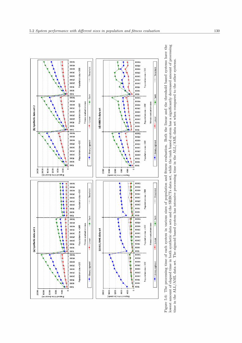
5.2 System performance with different sizes in population and fitness evaluation 130
Fig
ure
5.6
:T
he
pro
cess
ing
tim
eof
each
syst
emin
vari
ous
size
sof
popula
tion
and
fitn
ess
evalu
ati
on.
Both
the
linea
rand
the
thre
shold
base
dsy
stem
shav
eth
elo
wes
tam
ount
of
elapse
dti
me
inb
oth
synth
etic
data
sets
and
the
SR
BC
Ts
data
set,
while
the
tanh
base
dsy
stem
has
asi
gnifi
cantl
ydec
rease
dam
ount
of
pro
cess
ing
tim
ein
the
AL
L/A
ML
data
set.
The
sigm
oid
base
dsy
stem
has
inte
nsi
ve
pro
cess
ing
tim
ein
the
AL
L/A
ML
data
set
when
com
pare
dto
the
oth
ersy
stem
s.

5.3 The statistical significance of the extracted genes 131
5.2.4 Discussion
The findings reported in this section are based on the performance of each system in the effect of different
sizes in population and fitness evaluation . The results indicate that the integrity of the system in finding
stronger genes could, indeed, be compromised by inappropriate configuration of the GA population and the
fitness evaluation.
Cartwright (2008b) commented on, that the population size is not critically important in the success of a
GA,provided that the population size is not unreasonably small (i.e. < 40 chromosomes). Our results had
shown the importance of the population in the success of a GA and a strong interaction on the evolution
process, as is observed by DeJong and Spears (1991). This is indicated in the population size 100 with the
elevated processing time and low fitness accuracy achieved by each system in every fitness evaluation. With
the increased population size, better fitness performance and lower processing time are achieved when similar
fitness evaluations were applied. DeJong and Spears (1991) made such comments based on the augmentation
in the crossover operator and we derived similar conclusions with the increased fitness evaluation sizes.
In addition to the population size, a larger fitness evaluation also promise better fitness confidence in the
selected genes and the processing time is not always increased with larger evaluations. This is indicated in
Figure 5.6, where a lower or equal ratio of elapsed time was found in each fitness evaluation in population
sizes 200 and 300.
Despite the ideal population size, i.e. ranging from 40 to 100, as is suggested by Cartwright (2008b), our
results show that the population size 100 is still considerably small for handling microarray data sets. Based
on the ALL/AML and SRBCTs data sets, our findings suggest the minimal population size for microarray
data should be between 200 and 300. The minimal fitness evaluation size for binary class data should be
20000 and 25000 for multiclass data. The maximal fitness evaluation size should not be exceeds 40000. Our
findings also confirmed that the linear and the tanh based systems are the two most effective ANN activation
functions to be used to compute fitness values for GA chromosomes.
5.3 The statistical significance of the extracted genes
In this section, we examine the performance of each system based on the integrity of the extracted genes
by each system. This experiment was conducted based on the number of identified genes extracted in each
data set and is based on the population size 300 with fitness evaluation size ranging from 20000 to 40000.
Four tables based on these data sets were produced and each table presents a list of genes extracted by each
system, ordered, according to the selection frequency of the gene, along with its IG value. The IG (gain
ratio) method is a type of t-statistics approach that evaluates the significance of a feature by measuring the

5.3 The statistical significance of the extracted genes 132
gain ratio with respect to the class. This ratio value is used as the comparison on the feature ranking order
between the IG method and the GANN systems.
5.3.1 The synthetic data set 1
Table 5.1 on page 133 shows the list of extracted genes in the synthetic data set 1. All four systems have
identified all the 30 predefined genes in the data set with an identical set of the strongest genes, i.e. genes
5014 and 12; and the weakest genes, i.e. genes 15, 6, 5011 and 13. Amongst four systems, the threshold
based system, overall, has a fairly consistent ranking in the selected genes when the fitness evaluation size is
25000 or more (see Table 5.1d). Whilst the other three systems have a significant gene ranking discrepancy
in different sizes of fitness evaluations.
Both the sigmoid and the linear based systems have a significant ranking discrepancy in the fitness evaluation
size 40000 and the fitness evaluation size lesser than 40000. For sigmoid based system, as is showed in Table
5.1a, gene 5013 has been highly rated in smaller fitness evaluations, i.e. 20000 to 35000, however, this
gene is not frequently selected in the fitness evaluation size 40000. As opposed to gene 5013, gene 5008
has been highly rated in the fitness evaluation size 40000, but not in smaller fitness evaluations. For linear
based system in Table 5.1b, gene 5009 has a significant ranking in the fitness evaluation size 40000, when
compared to smaller fitness evaluations. The tanh based system, in Table 5.1c, however, has a greater
ranking discrepancy in the genes in the fitness evaluation size 35000 with the other evaluation sizes. The
differentially expressed genes involved genes 8, 5009 and 5008, for which gene 5009 was highly rated in the
fitness evaluation size 35000, however, genes 8 and 5008 were less significant.
By comparing the ranking order of the genes extracted by the GANN systems and the IG method, gene
5014 is the most significant gene (i.e. the primary feature for perfectly discriminate data classes) amongst
the 30 selected genes by all the GANN systems, followed by genes 12 and gene 13 is the weakest (i.e. the
least significant feature for class discrimination) in the ranking. The IG method, however, rated gene 12 as
the strongest with the rate of 0.612, followed by gene 5005 with the rate of 0.545 and gene 2 is the lowest
ranked in IG. The variability on the gene ranking is due to the IG method ranks genes based on its individual
significance to the cancer classes and overlooks its correlation with other genes to the cancer classes. The
GANN system, on the other hand, rank the genes based on its correlation with the other genes to the cancer
classes, meaning that using the selected genes by the GANN system. It is not sufficient for creating a perfect
discrimination between data classes compared to the genes selected by the IG method. However, the genes
selected by the GANN system provide more information on the correlation between expressed genes to the
cancer classes.
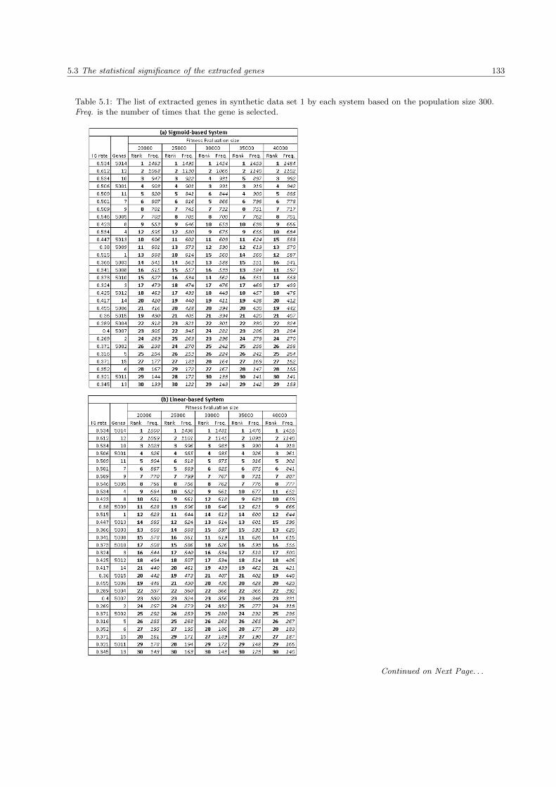
5.3 The statistical significance of the extracted genes 133
Table 5.1: The list of extracted genes in synthetic data set 1 by each system based on the population size 300.Freq. is the number of times that the gene is selected.
Continued on Next Page. . .

5.3 The statistical significance of the extracted genes 134
Table 5.1 – Continued
5.3.2 The synthetic data set 2
For synthetic data set 2 in Table 5.2, the linear based system outperforms the other three system by consis-
tently identifying 19 out of 30 predefined genes in the data set. Meanwhile, the sigmoid, the tanh and the

5.3 The statistical significance of the extracted genes 135
threshold based systems only identified 15, 14 and 18 predefined genes, respectively.
Table 5.2: The list of extracted genes in synthetic data set 2 by each system based on the population size 300.Freq. is the number of times that the gene is selected. Genes highlighted in red are noisy genes.
Continued on Next Page. . .

5.3 The statistical significance of the extracted genes 136
Table 5.2 – Continued
With increased fitness evaluation size, there was a significant improvement in the detection of the number
of predefined genes by each system. The sigmoid based system identified 18 predefined genes in the fitness
evaluation sizes 35000 and 40000, the linear based system detected 19 predefined genes in a fitness evaluation
size of 30000 or more, the tanh based system found 15 identical predefined genes in the fitness evaluation
sizes 30000 and 40000, and the threshold based system had the highest number of predefined genes found,
i.e. 20 genes, in the population size 35000. This would suggested that both the linear and the tanh based
systems required a minimal 30000 fitness evaluations for consistent and better selection performance, while
the sigmoid and the threshold based systems required at least 35000 fitness evaluations.
The findings also show that none of the systems was able to detect all the 30 predefined genes in synthetic
data set 2. This is because two different mean µ values, i.e. 20 stronger genes and 10 weaker genes, were used
in creating the data set. All systems are able to detect the stronger genes, but not the weaker genes as they
were ‘buried’ by the other stronger noisy genes, i.e. genes that were not suppose to be selected. Instead, the

5.3 The statistical significance of the extracted genes 137
presence of the noisy genes was detected in the sigmoid, the linear and the threshold based systems when the
fitness evaluation size was increased. These noisy genes are genes 667, 4883, 4377, 2828, 4175, 2816, 4390
and 2471. Gene 667 was found in the sigmoid based system when the fitness evaluation size was increased to
35000 or more (see Table 5.1a), genes 4377, 667, 2816 and 4175 were detected in the threshold based system
when higher fitness evaluation sizes were applied (see Table 5.1d) and genes 667, 4883 and 4377 appeared
in every fitness evaluation in the linear based system. This would suggested that the linear based system
can explore the most significant genes, even with smaller fitness evaluations, however, it cannot promise on
whether the selected genes are truly important to the subject of interest. The tanh based system is able
to rule out any unrelated genes from those that are highly related, however, it might also dismissed some
important genes.
By comparing the ranking order of the genes extracted by the GANN systems and the IG method, genes 21
and 12 are the most significant amongst the 30 selected genes all the GANN systems and for the IG method,
genes 12 (IG rate = 0.645) and 17 (IG rate = 0.248) are ranked as the most significant genes. Amongst the
predefined genes, the gene 22 (IG rate = 0.265) is the lowest ranked by the IG method. Meanwhile, for all
four GANN systems, gene 22 is more significant in terms of its correlation with other genes, compared to
gene 28 which is ranked lowly by the linear and the threshold based systems. For the sigmoid/tanh based
systems, gene 28 has not been identified as it’s correlated gene (i.e. gene 4377) has not been detected by
the systems. Amongst the noisy genes detected by the linear based system, genes 667 and 4883 provide a
certain level of statistical significance in the cancer classification based on the IG method and the other noisy
genes (4377, 2828, 4175, 2816, 4390 and 2471) pose no significance contribution to the cancer classification.
This means that the detection of these noisy genes is due to the detection of their correlated genes by the
linear based system. Gene 667 may correlates to the predefined genes 25, 13 and 14 based on the comparison
between the extracted genes by the sigmoid and the tanh based systems. The detection of gene 4377 is due
to the presence of gene 667 in the linear/threshold based systems.
5.3.3 The ALL/AML microarray data set
With reference on Table 5.3 on page 138 for ALL/AML data set, not surprisingly, the linear based system
has the highest number of extracted genes, i.e. 63 genes in total, and the tanh based system has the lowest
number of extracted genes, i.e. 53 genes in total. Both the sigmoid and the threshold based systems have,
in total, 54 genes extracted by the fitness evaluation size ranging from 20000 to 40000. Amongst the genes
extracted in each system, across the board, 39 genes overlapped in all systems, including the first-17 genes
selected by each system.

5.3 The statistical significance of the extracted genes 138
Table 5.3: The list of extracted genes in ALL/AML data set by each system based on the population size 300.Freq. is the number of times that the gene is selected. Genes highlighted in Boldface are common genes thatwere identified by all systems. Genes marked with “*” symbol are genes that matched with the genes reportedin the original study.
Continued on Next Page. . .

5.3 The statistical significance of the extracted genes 139
Table 5.3 – Continued
Continued on Next Page. . .

5.3 The statistical significance of the extracted genes 140
Table 5.3 – Continued
Continued on Next Page. . .

5.3 The statistical significance of the extracted genes 141
Table 5.3 – Continued
Both the sigmoid and the tanh based systems have 49 genes in common and have an identical set of the first-
11 selected genes. This might be due to both sigmoid and tanh based systems being non-linear functions,
which able to explore the correlation between features within the data. Furthermore, both the sigmoid and
the tanh based systems used the logistic curve (i.e. S-shape curve, see Figure 3.10 on page 81) for squashing
the activation value of each set of genes to a specific activation range before the output is generated by the
network. A logistic curve relates to the growth in the learning process. At the initial stage of the learning,
the growth is exponential, then as saturation begins (at the middle stage of the learning), the growth slows
and at the final stage of the learning (i.e. maturity), growth stops. This curve provides better discrimination

5.3 The statistical significance of the extracted genes 142
between data classes. Whilst, the linear and the threshold based systems have 52 common genes. This is
due to both systems performing simple linear computation on the activation value for each set of genes and
not squashing the activation results. Both the linear and the threshold functions utilised a straight line (see
Figure 3.10) to discriminate data classes rather than the logistic curve. However, they do not have genes in
identical rankings, mainly because the threshold based system restricted the activation of the network node
only when it exceeds the defined threshold value in the system.
A comparison between the genes extracted by each system and the original work by Golub et al. (1999)
was conducted (see Table 5.3). Amongst the selected genes in each system, both the sigmoid and the tanh
based systems have 20 genes, including the top 4-ranked genes in the systems, which were consistent with
the top-50 genes reported by Golub et al. Meanwhile, the linear and the threshold based system have 24
matching genes when compared to the reported genes by Golub et al. Amongst these common genes, 18 were
overlapped in all systems. This indicates that our method is effective in extracting informative genes from
ALL/AML data set and the data set is not being normalised. In Golub et al. (1999) work, the ALL/AML
data set had been normalised with zero mean and unit standard deviation. Some relevant works on the
ALL/AML data set is presented in Table C.1 in Appendix C.
By comparing the ranking order of the genes extracted by the GANN systems and the IG method, genes
1882, 2288, 4847 and 2354 are the top-4 most significant genes selected by both the sigmoid and the tanh
based systems, and these genes were consistent with the top-50 genes reported by Golub et al. (1999). For
the linear based system, the top-4 significant genes are 4847, 2288, 2354 and 2121, which were also consistent
with the top-50 genes reported by Golub et al.. Meanwhile the threshold based system identified gene 1779
as one of the top-4 important genes, instead of gene 2354 that was highly rated by the sigmoid, the linear
and the tanh based systems. For the IG method, the top-4 significant genes are 2288 and 760 (both genes
have the equal IG rate of. 0.747), 1882 (IG rate = 0.742), 4847 and 1834 (both genes have equal IG rate
of 0.735) and 3252 (IG rate = 0.718). Amongst the IG selected genes, gene 3252 is ranked in-between the
top-11 and the top-20 significant genes by all the GANN systems and gene 1834 is the least significant genes
in all the GANN systems as it does not have much correlation with other selected genes in the systems. For
gene 760, both the linear and the threshold based systems have poor ranking on this genes, however, in both
the sigmoid and the tanh based systems, gene 760 is ranked in-between the top-13 and the top-17 significant
genes. The gene ranking discrepancy between the sigmoid/tanh based systems and the linear/threshold
based systems confirmed our observation on the sigmoid and the tanh based systems in which the use of
logistic curve provides features which benefits data classification and simultaneously, these features pose a
certain degree of correlation with other selected features. The main reason for such gene ranking discrepancy
between GANN system and the IG method is due to the fact that the IG method measures the distance

5.3 The statistical significance of the extracted genes 143
between features to its nearest class independently, meaning that each of these features can be used as an
independent primary feature to categorise data classes as each feature provides a high classification accuracy
in the data set. Unlike the IG method, GANN explores the correlation between features to the data classes.
Therefore, a feature in the GANN system may not provides high classification accuracy in the data set;
however, using a group of features extracted by the GANN system, a certain level of classification accuracy
might be achieved.
5.3.4 The SRBCTs microarray data set
For SRBCTs data set in Table 5.4, surprisingly, both the sigmoid and the threshold based systems have the
highest number of extracted genes, i.e 70 genes in total, compared to the linear based system which has 69
extracted genes and the tanh based system which has extracted 68 genes from the data set. Amongst these
genes, 49 genes were overlapped in all systems, including the first-17 genes selected by each system. Both
the sigmoid and the tanh based systems have 61 genes in common, while the linear and the threshold based
systems have 65 common genes.
By comparing our findings with the original work conducted by Khan et al. (2001), the linear based system
has the lowest number of overlapping genes with the top 96 genes reported by Khan et al. Even though, the
top-10 ranked genes in all systems were consistent with the genes reported by Khan et al. Amongst the 69
genes identified by the linear based system, 39 genes were consistent with the genes reported by Khan et al.,
meanwhile, the sigmoid and the threshold based systems have 43 and 41 matching genes, respectively. The
tanh based system has the highest number of matching genes, i.e. 44 genes, to the genes reported by Khan
et al. Amongst these common genes, 34 were overlapped in all systems. This would suggest that the tanh
based system is the most effective system to be used in this study. Some relevant works on the SRBCTs
data set is presented in Table C.2 in Appendix C.
We also observed that more matching genes with the genes reported by Khan et al. were found in the fitness
evaluation size 35000.

5.3 The statistical significance of the extracted genes 144
Table 5.4: The list of extracted genes in SRBCTs data set by each system based on the population size 300.Freq. is the number of times that the gene is selected. Genes highlighted in Boldface are common genes thatwere identified by all systems. Genes marked with “*” symbol are genes that matched with the genes reportedin the original study.
Continued on Next Page. . .
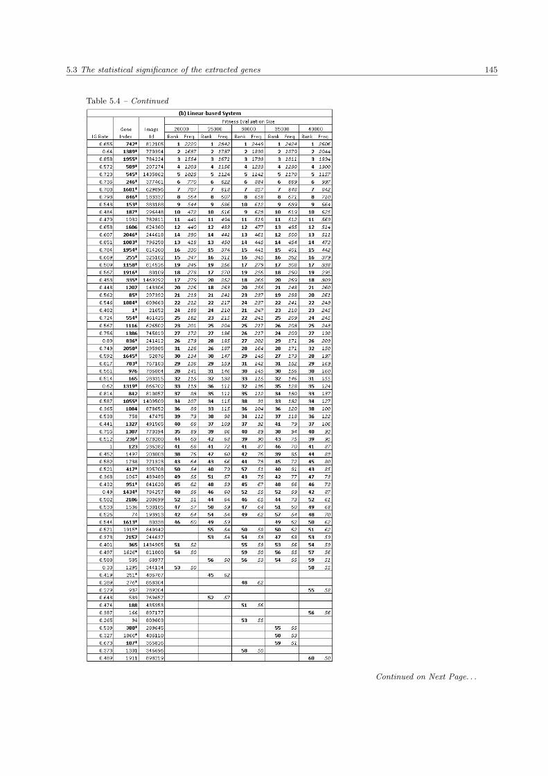
5.3 The statistical significance of the extracted genes 145
Table 5.4 – Continued
Continued on Next Page. . .
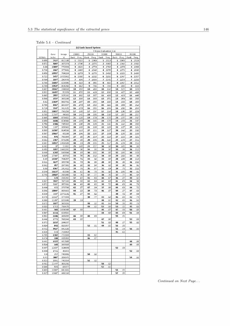
5.3 The statistical significance of the extracted genes 146
Table 5.4 – Continued
Continued on Next Page. . .

5.3 The statistical significance of the extracted genes 147
Table 5.4 – Continued
By comparing the ranking order of the genes extracted by the GANN systems and the IG method, common
genes 742, 1389, 509 and 1955 are the top-4 most significant genes selected by all the GANN systems and

5.3 The statistical significance of the extracted genes 148
these genes were matched with the top-96 genes reported by Khan et al. (2001). Genes 246, 545 and 187
were also highly ranked by both the sigmoid and the tanh based systems. Gene 545 was ranked at the 4th
place in both the linear and the threshold based systems. Using the IG method, the top-5 most significant
genes are genes 836 (IG rate = 0.89), 1955 (IG rate = 0.858), 1003 (IG rate = 0.851), 783 (IG rate = 0.817)
and 842 (IG rate = 0.814). Genes 742, 1389, 509 and 545 were lowly ranked by the IG method, with the IG
rates of 0.655, 0.64, 0.572 and 0.723, respectively. This is because these genes did not pose any classification
benefit when they were evaluated independently. Amongst the top-5 significant genes selected by the IG
method, gene 1003 is ranked in-between the top-11 to the top-20 significant genes by all GANN systems, and
the remaining genes 1003, 783 and 842 are lowly ranked by all GANN systems, meaning that these genes
does not have strong correlation with other selected genes. This shows that the GANN system was a better
approach for analysing microarray data as it explores the correlation between features in the data sets.
5.3.5 Discussion
The findings reported in this section are based on the performance of each system in extracting informative
genes in the effect of different fitness evaluations. For synthetic data sets, all systems have equivalent
performance in identifying all the 30 predefined genes in the synthetic data set 1. The linear based system
outperformed the other three system in the synthetic data set 2, by consistently identifying 18 out of 30
predefined genes in almost all fitness evaluation sizes. However, the linear based system also identified,
consistently, the highest number of noisy genes compared to both sigmoid and threshold based systems. The
tanh based system is the only system that did not select any noisy gene in the synthesis data set 2.
For microarray data sets, both linear and threshold based systems outperformed the sigmoid and the tanh
based systems in the ALL/AML data set by having 26 genes overlapped with the genes reported in the
original study. In the case of SRBCTs data set, the tanh based system outperformed the other three systems
with 44 matching genes to the original study. In terms of the number of extracted genes in the microarray
data, the linear based system, however, has the highest number of extracted genes in both data sets and the
tanh based system outperformed the other three system with the lowest number of extracted genes in both
microarray data sets.
The findings suggested that the tanh based system is, amongst all systems, the most effective systems to be
used for microarray data sets.

5.4 The biological sensible of the extracted genes 149
5.4 The biological sensible of the extracted genes
In Sections 5.1 and 5.2, we discussed the performance of each system based on different data sets: synthetic
data sets and microarray data sets, and the implication of two vital GA parameters: population and evolution;
to extract the most relevant genes from the respective data sets. Based on the findings in these sections, we
found that the sufficient population size for microarray studies should range from 200 to 300 and the fitness
evaluation sizes should range from 20000 to 40000.
This section presents a global view on the biological relevance of extracted genes presented in Section 5.3,
i.e. based on the population size 300 and the fitness evaluation sizes, ranging from 20000 to 40000. The
relevant studies of the disease will be reviewed and followed by a discussion on the gene findings of the GANN
prototype. A total of 74 and 90 genes extracted from the ALL/AML and SRBCTs data sets, respectively,
as is indicated in Tables 5.3 and 5.4 in Section 5.3 will be discussed.
In this section, the term “gene” indicates the identified features from the respective data sets and does not
possess biological context in the medical field. The term “chromosome’ represents a threadlike strand of
DNA in the nucleus of a biological cell.
5.4.1 The ALL/AML microarray data
Leukaemia is the blood cancer disease that is caused by the immaturity of blood cells in the bone marrow.
There are generally two main groups of leukaemia cancer, i.e. lymphoblastic leukaemia, derived from the
abnormal growth of lymphoblasts, these are the primitive progenitor cells originating in the bone marrow;
and myelogeneous leukaemia which arises from the immaturity of myeloid precursor cells in the bone marrow.
These two types of leukaemia cancer can be either chronic or acute. Due to the leukaemia data set that
we used in this thesis being acute leukaemia, we only discuss acute-based leukaemia cancers, i.e. Acute
Lymphoblastic Leukaemia (ALL) and Acute Myelogeneous Leukaemia (AML).
Leukaemia cancer is normally incurred by an abnormality of chromosomes in a cell. Several chromosomal
abnormalities has been reported in both ALL and AML which leads to tremendous advances in leukaemia
research. Most of the identified abnormalities involve translocation of different chromosomes in leukaemia
cells. Translocations is a type of “Structural Chromosomal Aberrations” that often cause human infertility
as they interfere with the normal distribution of chromosomes during meiosis (Robinson, 2003). In cancer
cases, it is a chromosome abnormality caused by re-arrangement of parts between two non-homogenous
chromosomes.
A standard designation t(A;B)(p1;q2) outlined by the International System for Human Cytogenetic Nomen-
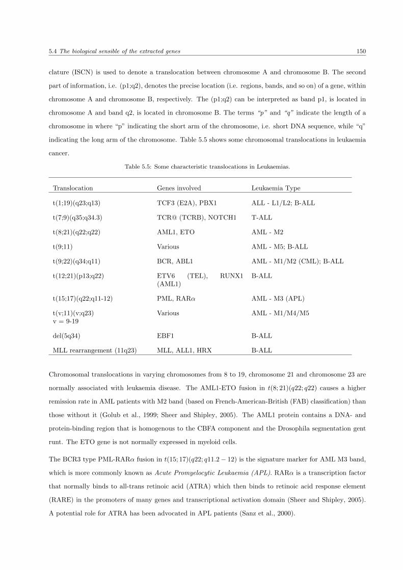
5.4 The biological sensible of the extracted genes 150
clature (ISCN) is used to denote a translocation between chromosome A and chromosome B. The second
part of information, i.e. (p1;q2), denotes the precise location (i.e. regions, bands, and so on) of a gene, within
chromosome A and chromosome B, respectively. The (p1;q2) can be interpreted as band p1, is located in
chromosome A and band q2, is located in chromosome B. The terms “p” and “q” indicate the length of a
chromosome in where “p” indicating the short arm of the chromosome, i.e. short DNA sequence, while “q”
indicating the long arm of the chromosome. Table 5.5 shows some chromosomal translocations in leukaemia
cancer.
Table 5.5: Some characteristic translocations in Leukaemias.
Translocation Genes involved Leukaemia Type
t(1;19)(q23;q13) TCF3 (E2A), PBX1 ALL - L1/L2; B-ALL
t(7;9)(q35;q34.3) TCR@ (TCRB), NOTCH1 T-ALL
t(8;21)(q22;q22) AML1, ETO AML - M2
t(9;11) Various AML - M5; B-ALL
t(9;22)(q34;q11) BCR, ABL1 AML - M1/M2 (CML); B-ALL
t(12;21)(p13;q22) ETV6 (TEL), RUNX1(AML1)
B-ALL
t(15;17)(q22;q11-12) PML, RARα AML - M3 (APL)
t(v;11)(v;q23)v = 9-19
Various AML - M1/M4/M5
del(5q34) EBF1 B-ALL
MLL rearrangement (11q23) MLL, ALL1, HRX B-ALL
Chromosomal translocations in varying chromosomes from 8 to 19, chromosome 21 and chromosome 23 are
normally associated with leukaemia disease. The AML1-ETO fusion in t(8; 21)(q22; q22) causes a higher
remission rate in AML patients with M2 band (based on French-American-British (FAB) classification) than
those without it (Golub et al., 1999; Sheer and Shipley, 2005). The AML1 protein contains a DNA- and
protein-binding region that is homogenous to the CBFA component and the Drosophila segmentation gent
runt. The ETO gene is not normally expressed in myeloid cells.
The BCR3 type PML-RARα fusion in t(15; 17)(q22; q11.2− 12) is the signature marker for AML M3 band,
which is more commonly known as Acute Promyelocytic Leukaemia (APL). RARα is a transcription factor
that normally binds to all-trans retinoic acid (ATRA) which then binds to retinoic acid response element
(RARE) in the promoters of many genes and transcriptional activation domain (Sheer and Shipley, 2005).
A potential role for ATRA has been advocated in APL patients (Sanz et al., 2000).

5.4 The biological sensible of the extracted genes 151
The Philadelphia (Ph) chromosome, i.e. BCR-ABL fusion in t(9; 22)(q34; q11) is commonly found in Chronic
Myelogeneous Leukaemia (CML) patients and AML patients in M1 and M2 subtypes. The immaturity of
the Ph chromosome can also occur in ALL (Sheer and Shipley, 2005). BCR gene encodes a serine kinase.
The ABL protein is a tyrosine kinase that contains a DNA binding domain and it functions as a negative
regulator of cell growth when the cell cycle is over-expressed.
A translocation between chromosomes 8 and 21 and a vary translocation of chromosomes varying from
9 to 19, may also possibly invoke AML. A translocation between chromosomes 8 and 21 will cause the
elevation of the c-myc activity, a gene involved in cell replication (Robinson, 2003). A translocation between
chromosomes 9 and 19 contributes to the AML patients with M1, M4 and M5 bands.
Deletion of the gene EBF1 in del(5q34), an early B-cell factor, could also contribute to leukaemogenesis
(Mullighan et al., 2007). The EBF1 gene is required for the development of B-cells and with the gene TCF3
regulates the expression of B-lineage genes.
In addition to chromosomal translocations, up-regulation of certain genes expressed in leukaemia cells is due
to chromosomal rearrangement and could contribute to the development of the cancer.
The positive expression in the genes CD1, CD3, CD4, CD8 and terminal deoxynucleotidyl transferase (TdT)
correspond to an intermediate thymocyte stage of T-cell ALL differentiation (Strauchen, 2001). The expres-
sion of TdT is normally restricted to lymphoid precursors, especially in T-cell and the non-positive TdT
(i.e. suppressed) might be detected in B-cells when it is associated with the down-regulation of genes CD10
and CD34; a high WBC count and the rearrangement of gene MLL (Mixed Lineage Leukaemia) (Liu et al.,
2004b).
Regulation of the gene CD179a/b in chromosome 22 is useful as a marker for differentiating the immature
and mature B-cell precursors, in which the up-regulation of genes CD179a/b were specifically expressed in
precursor B-cell lymphoblastic lymphomas, but not in mature B-cell lymphomas of childhood (Kiyokawa
et al., 2004).
Suppression in the gene myeloperoxidase (MPO) in adult ALL patients reduces the survival rate of the
patient (Arber et al., 2001).
The gene podocalyxin, a CD34 family member, is a useful hematopoietic blast marker for patients with
abnormal hematopoietic cells. The increased level of podocalyxin is commonly expressed in both AML and
ALL, as well as in cutaneous myeloid sarcoma disease (Kelley et al., 2005).
The translocations in chromosomes with t(8;21) is a distinct clinicopathologic entity for patients who have
been diagnosed with AML cancer (Khoury et al., 2004). The translocations t(8;21) displayed a higher level
of CD34, HLA-DR and MPO expression, and a lower level of CD13 and CD33 expression.

5.4 The biological sensible of the extracted genes 152
The gene CD99 (MIC2) is characteristically expressed in precursor B- and T-cell lymphoblastic leukaemias
and lymphomas, as well as in Ewing sarcoma and primitive neuroectodermal tumours (Kang and Dunphy,
2006). It is most intensely expressed by immature thymus T-lineage cells and in the earliest stage of precursor
B-cells.
A total of 74 genes were extracted from the ALL/AML data set. Among 74 genes, 39 genes were found by
all systems, 6 were found by 3 systems (i.e. 4 in sigmoid/linear/tanh based; 2 in sigmoid/tanh/threshold
based), 21 genes were identified by 2 systems (i.e. 6 in sigmoid/tanh based; 11 in linear/threshold based;
2 in linear/tanh based; 2 in sigmoid/linear based), 3 genes were identified by only the linear based system,
3 genes by the tanh based system and 2 genes by the threshold based system. Table 5.6 presents all 74
extracted genes ordered by the cytoband of the gene. The complete list of the genes extracted by each
system is presented in Table 5.3 on page 138. The correlation between genes within the sample and the gene
interaction within the sample is presented in Figure 5.7.
Table 5.6: The summary list of ALL/AML genes. The genes are ordered according to the cytoband of theselected gene. The Index denotes the row number of the selected gene. The Gene Accession is the id numberof the selected gene. The Symbol represents the official abbreviation of the selected gene based on the NCBIGenbank (as of October 2009). The GeneID is the NCBI genbank number of the selected gene. The Cytobandis the location of the selected gene. The Group is the cancer group to which the selected gene belongs. Genesmarked with “§” are genes that were match with the genes reported by Golub et al. (1999). Genes marked with“†” were genes identified by all systems in the GANN prototype.
Index Gene Accession Symbol GeneID Cytoband Group
Index 6510 U23852 LCK 3932 1p34.3 ALL
Index 804 HG1612-HT1612† MARCKSL1 65108 1p35.1 ALL
Index 1928 M31303†§ STMN1 3925 1p36.1-p35 ALL
Index 5445 X04526 GNB1 2782 1p36.33 ALL
Index 4095 X06948 FCER1A 2205 1q23 AML
Index 6388 S54005 TMSB10 9168 2p11.2 ALL
Index 2408 M96803 SPTBN1 6711 2p21 ALL
Index 4291 X56468 YWHAQ 10971 2p25.1 ALL
Index 6184 M26708 PTMA 5757 2q35-q36 ALL
Index 5501 Z15115†§ TOP2B 7155 3p24 ALL
Index 412 D42043† RFTN1 23180 3p24.3 ALL
Index 668 D86967† EDEM1 9695 3p26.2 ALL
Index 760 D88422† CSTA 1475 3q21 AML
Index 6200 M28130†§ IL8 3576 4q13-q21 AML
Index 6201 Y00787†§ IL8 3576 4q13-q21 AML
Index 7128 M71243 GYPA 2993 4q28.2-q31.1 AML
Index 5952 U05255 GYPB 2994 4q28-q31 AML
Index 6796 J02982 GYPB 2994 4q28-q31 AML
Index 5950 M29610† GYPE 2996 4q31.1 AML
Continued on Next Page. . .

5.4 The biological sensible of the extracted genes 153
Table 5.6 – Continued
Index Gene Accession Symbol GeneID Cytoband Group
Index 1630 L47738§ CYFIP2 26999 5q33.3 ALL
Index 3258 U46751§ SQSTM1 8878 5q35 AML
Index 3320 U50136§ LTC4S 4056 5q35 AML
Index 2354 M92287†§ CCND3 896 6p21 ALL
Index 4409 X64594 RHAG 6005 6p21.1-p11 AML
Index 4438 X66401 TAP1/TAP2 6890/6891 6p21.3 ALL
Index 6049 U89922† LTB 4050 6p21.3 ALL
Index 5772 U22376†§ MYB 4602 6q22-q23 ALL
Index 4211 X51521† EZR 7430 6q25.2-q26 ALL
Index 4847 X95735†§ ZYX 7791 7q32 AML
Index 1745 M16038†§ LYN 4067 8q13 AML
Index 6539 X85116§ STOM 2040 9p34.1 AML
Index 1941 M31994 ALDH1 216 9q21.13 AML
Index 1144 J05243 SPTAN1 6709 9q33-q34 ALL
Index 4196 X17042†§ SRGN 5552 10q22.1 AML
Index 1685 M11722† DNTT 1791 10q23-q24 ALL
Index 4229 X52056 SPI1 6688 11p11.2 AML
Index 3984 U94855 EIF3F 8665 11p15.4 ALL
Index 1962 M33680† CD81 975 11p15.5 ALL
Index 2121 M63138†§ CTSD 1509 11p15.5 AML
Index 6702 X97267 PTPRCAP 5790 11q13.3 ALL
Index 4050 X03934 CD3D 915 11q23 ALL
Index 6041 L09209† APLP2 334 11q23-q25—11q24 AML
Index 3252 U46499† MGST1 4257 12p12.3-p12.1 AML
Index 4377 X62654† CD63 967 12q12-q13 AML
Index 1239 L07633† PSME1 5720 14q11.2 ALL
Index 1809 M21624 TRD@ 6964 14q11.2 ALL
Index 4328 X59417†§ PSMA6 5687 14q13 ALL
Index 4680 X82240 TCL1A 8115 14q32.1 ALL
Index 2020 M55150§ FAH 2184 15q23-q25 AML
Index 6225 M84371 CD19 930 16p11.2 ALL
Index 2111 M62762§ ATP6V0C 527 16p13.3 AML
Index 4951 Y07604† NME4 4833 16p13.3 AML
Index 6271 M33493 TPSAB1 7177 16p13.3 AML
Index 1975 M34344† ITCA2B 3674 17q21.32 AML
Index 4373 X62320† GRN 2896 17q21.32 AML
Index 6079 U59632† SEPT4 5414 17q22-q23 AML
Index 2335 M89957 CD79B 974 17q23 ALL
Continued on Next Page. . .

5.4 The biological sensible of the extracted genes 154
Table 5.6 – Continued
Index Gene Accession Symbol GeneID Cytoband Group
Index 1779 M19507† MPO 4353 17q23.1 AML
Index 6215 M19508 MPO 4353 17q23.1 AML
Index 5542 M37271 CD7 924 17q25.2-q25.3 ALL
Index 5543 D00749 CD7 924 17q25.2-q25.3 ALL
Index 2642 U05259†§ CD79A 973 19p13.2 ALL
Index 7119 U29175§ SMARCA4 6597 19p13.2 ALL
Index 2288 M84526†§ CFD 1675 19p13.3 AML
Index 2402 M96326†§ AZU1 566 19p13.3 AML
Index 6855 M31523†§ TCF3 6929 19p13.3 ALL
Index 1796 M20902† APOC1 341 19q13.2 AML
Index 1834 M23197†§ CD33 945 19q13.3 AML
Index 1674 M11147 FTL 2512 19q13.3 AML
Index 1882 M27891†§ CST3 1471 20p11.21 AML
Index 1704 M13792§ ADA 100 20q12-q13.11 ALL
Index 1829 M22960† CTSA 5476 20q13.1 AML
Index 758 D88270† IGL@ 3535 22q11.1-q11.2 AML
Index 6376 M83652†§ CFP 5199 Xp11.3-p11.23 AML
Amongst the 74 identified genes, 35 were expressed in ALL class and the remaining 39 genes were expressed
in AML class.
The already proven efficient biomarkers from the existing medical studies that were involved in the translo-
cations were found by the GANN prototype. These biomarkers are DNTT (Index 1685, previously known
as TdT), SMARCA4 (Index 7119), TCF3 (Index 6855), CD3D (Index 4050), CD79 (Index 2642 and In-
dex 2335), MPO (Index 1779 and Index 6215) and APLP2 (Index 6041). The genes DNTT, SMARCA4 and
TCF3 were reported as being under-expressed in an MLL translocation (Armstrong et al., 2002). Amongst
these biomarkers, 5 were found by all systems (i.e. Index 1685, Index 6855, Index 2642, Index 1779 and
Index 6041) and the remaining 2 were identified by multiple systems (i.e. Index 7119 in linear/tanh based
and Index 2335 in sigmoid/linear/tanh based). Please refer to Table 5.3 on page 138 for the complete list of
the extracted genes by each system.
DNTT (Index 1685) plays a role in DNA repair and is normally expressed in the normal and the early stage
of malignant B-cell development. It was expressed in some B-cell ALL samples in Figure 5.7 which suggests
that these samples were taken at the early stage of B-ALL development.
SMARCA4 (Index 7119) is a SWI/SNF family member, is a tumour suppression gene that interacts with
the tumour suppression gene p53, for p53-driven transcriptional activation and it plays an important role in
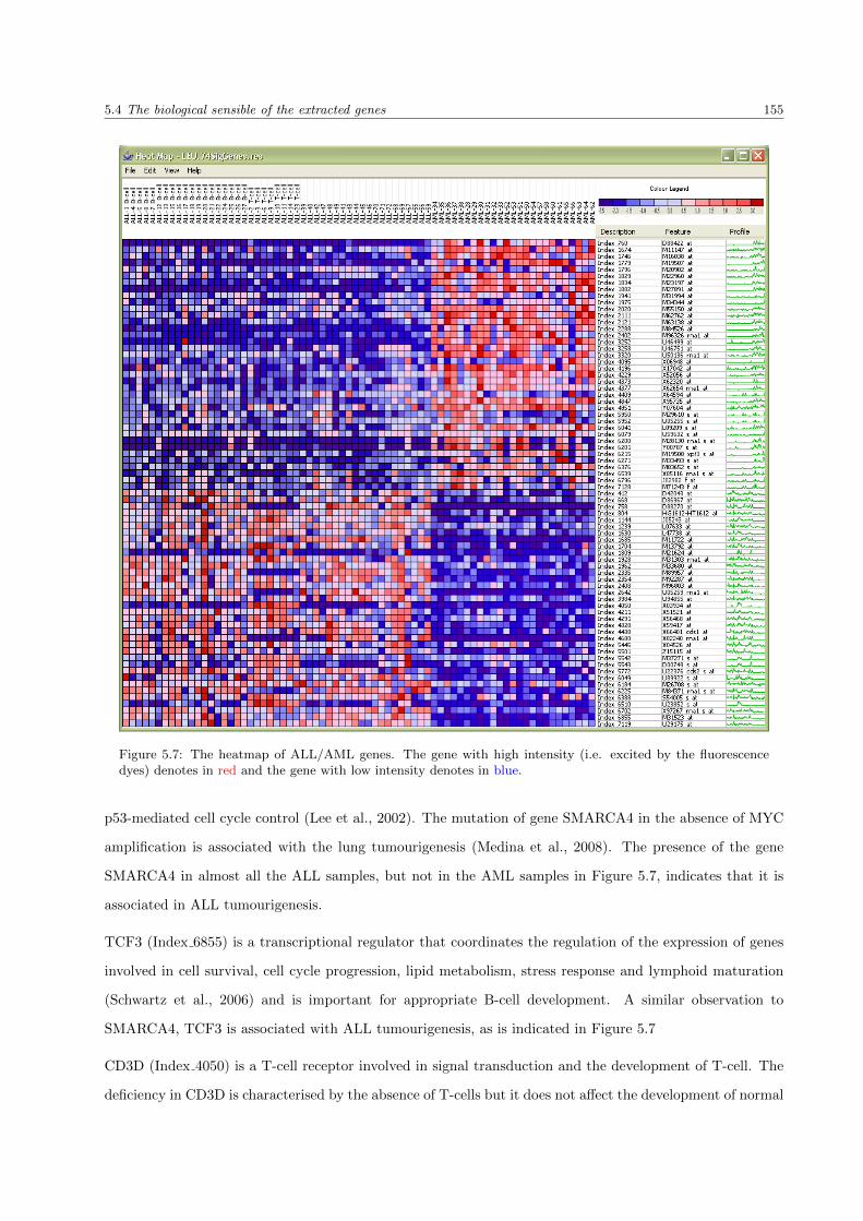
5.4 The biological sensible of the extracted genes 155
Figure 5.7: The heatmap of ALL/AML genes. The gene with high intensity (i.e. excited by the fluorescencedyes) denotes in red and the gene with low intensity denotes in blue.
p53-mediated cell cycle control (Lee et al., 2002). The mutation of gene SMARCA4 in the absence of MYC
amplification is associated with the lung tumourigenesis (Medina et al., 2008). The presence of the gene
SMARCA4 in almost all the ALL samples, but not in the AML samples in Figure 5.7, indicates that it is
associated in ALL tumourigenesis.
TCF3 (Index 6855) is a transcriptional regulator that coordinates the regulation of the expression of genes
involved in cell survival, cell cycle progression, lipid metabolism, stress response and lymphoid maturation
(Schwartz et al., 2006) and is important for appropriate B-cell development. A similar observation to
SMARCA4, TCF3 is associated with ALL tumourigenesis, as is indicated in Figure 5.7
CD3D (Index 4050) is a T-cell receptor involved in signal transduction and the development of T-cell. The
deficiency in CD3D is characterised by the absence of T-cells but it does not affect the development of normal

5.4 The biological sensible of the extracted genes 156
B-cells (Dadi et al., 2003). This observation is also indicated in Figure 5.7 where CD3D is highly expressed in
all the T-ALL samples and in a B-ALL sample. This may suggest that possibly combined immunodeficiency
genes in the B-ALL induce the activation of the CD3D receptor.
CD79A (Index 2642) and CD79B (Index 2335) are B lymphocyte antigen receptors required for the de-
velopment of normal B-cells. The down-regulation of both CD79 genes are the hallmark of tumoural B
lymphocytes in B-cell chronic lymphocytic leukaemia (Vuillier et al., 2005) and the coexpression of CD79A
with AML1/ETO fusion in t(8;21) represents biphenotypic acute leukaemia (He et al., 2007). Both CD79A
and CD79B have expressed a moderate level in all ALL samples in Figure 5.7 but not in T-ALL samples.
APLP2 (Index 6041) belongs to the APP family that may assist in the regulation of haemostasis. This is
indicated by the presence of APLP2 in most AML samples in Figure 5.7.
MPO (Index 1779 and Index 6215) is a key enzyme in the cellular response to hypoxia and consequent
development of tissue fibrosis (Saed et al., 2009). The gene MPO is presented during abnormal myeloid cell
differentiation. The high level of MPO in some AML samples in Figure 5.7 suggests the possibilities of the
AML subgroups in the AML class.
In addition to the biomarkers, there are also genes which are only expressed in one of the subgroups of ALL.
These genes includes genes that are only expressed in T-ALL, i.e. ADA (Index 1704) and CD7 (Index 5542
and Index 5543) and genes that are only expressed in B-ALL, i.e. IGL@ (Index 758), CD19 (Index 6225)
and TCL1A (Index 4680). These genes could be potential signature markers in differentiating T-ALL and
B-ALL. Amongst these genes, excepting Index 758 that was found by all systems, 3 were overlapped in
sigmoid/tanh based systems (i.e. Index 1704, Index 5543 and Index 4680), Index 6225 in the linear based
system and Index 5542 was solely identified by the tanh based system with the fitness evaluation size 25000
(see Table 5.3 on page 138).
ADA (Index 1704) catalyses the hydrolysis of adenosine to inosine. The deficiency in this gene could causes
a dysfunction of both B and T lymphocytes with the impairment of cell immunity and decreased production
of immunologlobulins (EntrezGene: GeneID 100). The elevation of this gene may activate the Th1 response
to the disease (Kisacik et al., 2009) and have been associated with congenital haemolytic anaemia. The
gene CD7 (Index 5542 and Index 5543) is the immunoglobulin superfamily member that is normally found
on thymocytes and mature T-cells. It is required in T-cell interactions and also in T-cell/B-cell interaction
during early lymphoid development (EntrezGene: GeneID 924).
IGL@ (Index 758) plays an important role in B-cell development. It contains lambda light chain in the
germline organisation which allows it to recognise foreign antigens and to initiate immune responses (En-
trezGene: GeneID 3535). CD19 (Index 6225) encodes the cell surface molecule which binds with the antigen

5.4 The biological sensible of the extracted genes 157
receptor of B lymphocytes to decrease the threshold for antigen receptor-dependent stimulation (Entrez-
Gene: GeneID 930). It is constantly expressed in all stages of B lineage differentiation and is a reliable
marker for diagnosing B-lineage ALL (Chen et al., 2004). TCL1A (Index 4680) is a powerful oncogene that
is involved in the pathogenesis of mature T-cell leukaemia (Pekarsky et al., 2004). It plays an important role
in controlling the growth and the effector T-cell functions (Hoyer et al., 2005). In Figure 5.7, TCL1A is not
expressed in T-ALL samples, but in most B-ALL samples, which could suggests that the T-ALL samples
in the ALL/AML data set are premature, i.e. in the early stages of T-cell development and TCL1A is
predominantly associated with mature precursor lymphocytes but not differentiated B- or T-cells.
Amongst the identified genes, some genes may be involved in some known leukaemia chromosomal aber-
rations. These genes include E2A/PBX1 fusion related genes, i.e. FCER1A (Index 4095), SMARCA4
(Index 7119), CFD (Index 2288), AZU1 (Index 2402), TCF3 (Index 6855), APOC1 (Index 1796), CD33 (In-
dex 1834) and FTL (Index 1674); TCR/NOTCH1 fusion related gene, i.e. SPTAN1 (Index 1144); BCR/ABL1
fusion related genes, i.e. SPTAN1 (Index 1144) and IGL@; MLL rearrangement genes, i.e. CD3D (In-
dex 4050) and APLP2 (Index 6041).
The findings in this study shows that the GANN prototype is a robust feature extraction method that is able
to extract highly informative genes from the raw (unprocessed) data set. This is indicated by the majority of
the identified genes involved in leukaemogenesis and also some signature genes in differential B- and T-ALL.
The tanh based system outperformed the other three systems to extract the biological significant genes from
the data set.
5.4.2 The SRBCTs microarray data
The term “Small round blue cell tumours” (SRBCTs) is a generic name (category) used to describe a large
number of malignant tumours that occur in childhood in the medical studies. They are characterised by
small, round and relatively undifferentiated cells, such as Ewing’s sarcoma, acute leukaemia, small cell
mesothelioma, neuroblastoma, rhabdomyosarcoma, synovial sarcoma, Non-Hodgkin’s lymphoma and many
more small round cells. In this thesis, we examine only four types of SRBCTs tumours, which are Burkitt’s
Lymphoma (NB), a subtype of Non-Hodgkin’s Lymphoma, Ewing’s Sarcoma (EWS), Neuroblastoma (NB)
and Rhabdomyosarcoma (RMS).
Burkitt’s lymphoma (BL) is a cancer yielded from the dysfunction of B lymphocytes, a type of white blood
cell. This cancer is associated with the translocation of the c-myc gene with other genes, such as the
translocation between c-myc gene with genes located in chromosome 14, i.e. t(8;14)(q24;32). The c-myc
gene plays an important role in cell cycle progression and its dysfunctional, i.e. mutation, over-expression,
rearrangement and translocation, are associated with a variety of haematopoietic malignancy (EntrezGene:

5.4 The biological sensible of the extracted genes 158
GeneID 4609).
Ewings sarcoma (EWS) is a bone malignant cancer that predominantly occurs in the second decade of life and
commonly affects areas including the pelvis, the femur, the humerus and the ribs (Rajwanshi et al., 2009).
The cell origin of this tumour is uncertain. EWS has a shared cytogenetic abnormality with the primitive
neuroectodermal tumour (PNET) which is a small round cell malignancy that arises from the soft tissue or
bone. The shared cytogenetic abnormality involves a translocation between chromosome 11 and chromosome
22, i.e. the EWS/FLI1 fusion in t(11;22)(q24;q12), a signature marker for EWS/PNET from other small
round tumours (Owen et al., 2008). The EWS (EWSR1) gene acts as a strong transcriptional activator in
various cellular processes and chromosomal translocations between this gene and other transcriptional factor
genes could result in the production of chimeric proteins that are involved in tumourigenesis. The FLI1 gene
is a member of ETS transcription factor that is involved in a wide variety of bodily regulation functions,
including cell differentiation, cell cycle control, cell migration, cell proliferation, apoptosis and angiogenesis.
The EWS/FLI1 fusion can be detected by the positive expression of CD99 (Rajwanshi et al., 2009) and
the negative expression of CD45 (Bernsteina et al., 2006). Other less frequent translocations involved in
this tumour are the EWS/ERG fusion in t(21;22) (Sorensen et al., 1994) and the EWS/ETV1 fusion in
t(7;22)(p22;q12) (Jeon et al., 1995).
Neuroblastoma (NB) is the third most common, solid malignant tumour of infancy and childhood that
predominantly occur in the male group (Rajwanshi et al., 2009). This tumour arises from the neuroblasts
which are the undifferentiated precursor cells of the sympathetic nervous system. The etiology of NB is
not well understood by medical scientists, however, there are cases where this tumour could be inherited
from a parent and is associated with the mutation of the germline in the ALK gene (Mosse et al., 2008) at
chromosome band 2p23. The ALK gene plays an important role in the development of the brain and exerts
its effects on specific neurons in the nervous system. The presence of del(1p), i.e. deletion of chromosome
1 short arm, or MYCN amplification are also useful in detecting the early stage of NB development in the
young age group (Sheer and Shipley, 2005).
Rhabdomyosarcoma (RMS) is a connective tissue related cancer that commonly occurs in children (Rajwan-
shi et al., 2009). This tumour can be classified into three main subtypes: embryonal rhabdomyosarcoma
(ERMS), alveolar rhabdomyosarcoma (ARMS) and pleomorphic rhabdomyosarcoma (PRMS). The former
two subtypes of RMS are almost undifferentiated based on the morphological result, however, at a molecu-
lar level, ARMS shows predominantly dissociated cells or chance formations and ERMS shows large tissue
fragments with abundant eosinophilic material and disassociated cells (Rajwanshi et al., 2009). The Desmin
protein has been reported as a useful marker for detecting large rhabdomyoblasts during the early differ-
entiation of skeletal and smooth muscle cells, however, it is also positively expressed in smaller, less well

5.4 The biological sensible of the extracted genes 159
differentiated tumour cells (Rajwanshi et al., 2009). The other two markers: MyoD1 and myogenin, have
a higher sensitivity (positive) than desmin in RMS detection and they can differentiate ARMS from the
embryonal type (Rajwanshi et al., 2009). The MyoD1 gene involves in muscle regeneration and regulates
muscle cell differentiation. The myogenin (MYOG) gene is a muscle-specific transcription factor that is
essential in the development of functional skeletal muscle. Table 5.7 shows some cytogenetic differentiation
in four types of SRBCTs tumours.
Table 5.7: Some cytogenetic differentiation in four types of SRBCTs.
Cytogenetic Difference Genes involved Tumour Type
t(8;14)(q24;q32) c-myc (MYC), IGH@ BL
c-myc rearrangement c-myc (MYC) BL
t(11;22)(q24;q12) EWS (EWSR1), FLI1 EWS
t(21;22)(q22;q12) EWS (EWSR1), ERG EWS
t(7;22)(p22;q12) EWS (EWSR1), ETV1 EWS
+CD99, −CD45 CD99, CD45 EWS
ALK mutation ALK NB
del(1p) Various NB
+DES, +MYOD1, +MYOG DES, MYOD1, MYOG RMS
A total of 90 genes were extracted from the SRBCTs data set. Among these 90 genes, 49 genes were
found by all systems, 11 genes were found by 3 systems (i.e. 6 in sigmoid/linear/tanh based; 4 in sig-
moid/tanh/threshold based; 1 in linear/tanh/threshold based), 18 genes were identified by 2 systems (i.e.
7 in linear/threshold based; 8 in sigmoid-/tanh-based and 1 in linear/tanh based) and 12 were detected by
individual system (i.e. 3 by sigmoid based system, 3 by linear based system, 5 by tanh based system and 1
by threshold based system). Table 5.8 presents all 90 extracted genes ordered by the cytoband of the gene.
The complete list of these 90 genes is presented in Table 5.4 in page 144. The correlation between genes
within the sample and the gene interaction to the sample is presented in Figure 5.8.
Table 5.8: The summary list of SRBCTs. The genes are ordered according to the cytoband of the selectedgene. The Index denotes the row number of the selected gene. The Img Id is the clone number of the selectedgene. The Symbol represents the official abbreviation of the selected gene based on the NCBI Genbank (as ofOctober 2009). The GeneID is the NCBI genbank number of the selected gene. The Cytoband is the location ofthe selected gene. The Group is the cancer group to which the selected gene belongs. Genes marked with “§”are genes that were match with the genes reported by Khan et al. (2001). Genes marked with “†” were genesidentified by all systems in the GANN prototype.
Index Img Id Symbol GeneID Cytoband Group
Index 251 486787§ CNN3 1266 1p22-p21 RMS/NB (<> BL)
Continued on Next Page. . .

5.4 The biological sensible of the extracted genes 160
Table 5.8 – Continued
Index Img Id Symbol GeneID Cytoband Group
Index 1700 796475 FHL3 2275 1p34 EWS/RMS (<> BL/NB)
Index 1738 771323 PLOD1 5351 1p36.22 RMS
Index 742 812105†§ MLLT11 10962 1q21 NB (<> BL)
Index 1613 80338†§ SELENBP1 8991 1q21-q22 EWS (<> BL/NB)
Index 129 298062§ TNNT2 7139 1q32 RMS
Index 1067 489489 LBR 3930 1q42.1 BL
Index 1434 784257†§ KIF3C 3797 2p23 NB (<> BL)
Index 1662 377048§ MYO1B 4430 2q12-q34 NB (<> BL)
Index 2144 308231§ MYO1B 4430 2q12-q34 NB (<> BL)
Index 1105 788107§ BIN1 274 2q14 RMS (<> BL)
Index 566 357031§ TNFAIP6 7130 2q23.3 EWS
Index 783 767183†§ HCLS1 3059 3q13 BL
Index 1764 44563§ GAP43 2596 3q13.1-q13.2 NB
Index 2199 135688§ GATA2 2624 3q21.3 NB (<> BL)
Index 1066 486110§ PFN2 5217 3q25.1-q25.2 NB
Index 589 769657 PPP1R2 5504 3q29 BL
Index 236 878280†§ CRMP1 1400 4p16.1-p15 NB (<> BL)
Index 1319 866702†§ PTPN13 5783 4q21.3 EWS
Index 1601 629896†§ MAP1B 4131 5q13 NB (<> BL)
Index 1 21652†§ CTNNA1 1495 5q31 EWS/RMS (<> BL)
Index 1721 40643 PDGFRB 5159 5q31-q32 EWS/RMS (<> BL)
Index 1955 784224†§ FGFR4 2264 5q35.1-qter RMS
Index 188 435953† ITPR3 3710 6p21 BL/EWS (<> NB)
Index 1932 782811 HMGA1 3159 6p21 BL
Index 1606 624360† PSMB8 5696 6p21.3 BL
Index 1634 82903 TAPBP 6892 6p21.3 BL/EWS
Index 1915 840942§ HLA-DPB1 3115 6p21.3 BL
Index 1916 80109†§ HLA-DQA1 3117 6p21.3 BL
Index 2186 208699† KIAA1949 170954 6p21.3 BL
Index 846 183337†§ HLA-DMA 3108 6p21.3 BL
Index 1536 530185 CD83 9308 6p23 BL (<> RMS)
Index 407 195751 AKAP7 9465 6q23 EWS
Index 1327 491565† CITED2 10370 6q23.3 EWS (<> BL)
Index 165 283315† PGAM2 5224 7p13-p12 BL (<> RMS)
Index 1884 609663†§ PRKAR2B 5577 7q22 BL (<> RMS)
Index 1084 878652† PMS2L12 392713 7q22.1 NB (<> BL)
Index 246 377461†§ CAV1 857 7q31.1 EWS
Index 1911 898219 MEST 4232 7q32 RMS (<> BL)
Continued on Next Page. . .

5.4 The biological sensible of the extracted genes 161
Table 5.8 – Continued
Index Img Id Symbol GeneID Cytoband Group
Index 951 841620†§ DPYSL2 1808 8p22-p21 EWS/NB (<> BL)
Index 74 193913 LYN 4067 8q13 BL
Index 107 365826†§ GAS1 2619 9q21.3-q22 EWS/RMS (<> BL/NB)
Index 1645 52076†§ NOE1 10439 9q34.3 EWS (<> BL/RMS)
Index 276 868304§ ACTA2 59 10q23.3 BL
Index 166 897177 PGAM1 5223 10q25.3 BL (<> RMS)
Index 417 395708†§ DPYSL4 10570 10q26 NB (<> BL)
Index 139 729964 SMPD1 6609 11p15.4-p15.1 EWS/RMS
Index 1207 143306† LSP1 4046 11p15.5 RMS
Index 187 296448†§ IGF2 3481 11p15.5 RMS
Index 509 207274†§ IGF2 3481 11p15.5 RMS
Index 1386 745019† EHD1 10938 11q13 BL
Index 1980 841641§ CCND1 595 11q13 EWS/NB (<> BL)
Index 1263 324494§ HSPB2 3316 11q22-q23 RMS (<> BL/NB)
Index 1991 740554 RDX 5962 11q23 EWS (<> BL)
Index 842 810057† CSDA 8531 12p13.1 <>NB
Index 1301 346696 TEAD4 7004 12p13.3-p13.2 RMS (<> BL)
Index 836 241412†§ ELF1 1997 13q13 BL
Index 1387 740604† ISG20 3669 15q26 BL
Index 1497 203003 NME4 4833 16p13.3 EWS/NB (<> BL)
Index 85 297392†§ MT1L 4500 16q13 BL
Index 585 68977 PSMB10 5699 16q22.1 BL
Index 153 383188†§ RCVRN 5957 17p13.1 NB (<> BL)
Index 430 379708 CHD3 1107 17p13.1 EWS (<> BL)
Index 1003 796258†§ SGCA 6442 17q21 RMS
Index 365 1434905† HOXB7 3217 17q21.3 EWS (<> BL/NB)
Index 976 786084† CBX1 10951 17q21.32 NB
Index 554 461425†§ MYL4 4635 17q21-qter RMS
Index 1626 811000§ LGALS3BP 3959 17q25 EWS/NB (<> BL)
Index 255 325182†§ CDH2 1000 18q11.2 NB
Index 1954 814260†§ KDSR 2531 18q21.3 EWS
Index 368 1473131§ TLE2 7089 19p13.3 EWS (<> BL/NB)
Index 847 265874 NFIC 4782 19p13.3 EWS
Index 380 289645†§ APLP1 333 19q13.1 EWS/NB (<> BL)
Index 257 740801 BCKDHA 593 19q13.1-q13.2 EWS (<> BL)
Index 1389 770394†§ FCGRT 2217 19q13.3 EWS
Index 1055 1409509†§ TNNT1 7138 19q13.4 RMS (<> BL)
Index 1158 814526†§ RBM38 55544 20q13.31 RMS/BL (<> NB)
Continued on Next Page. . .
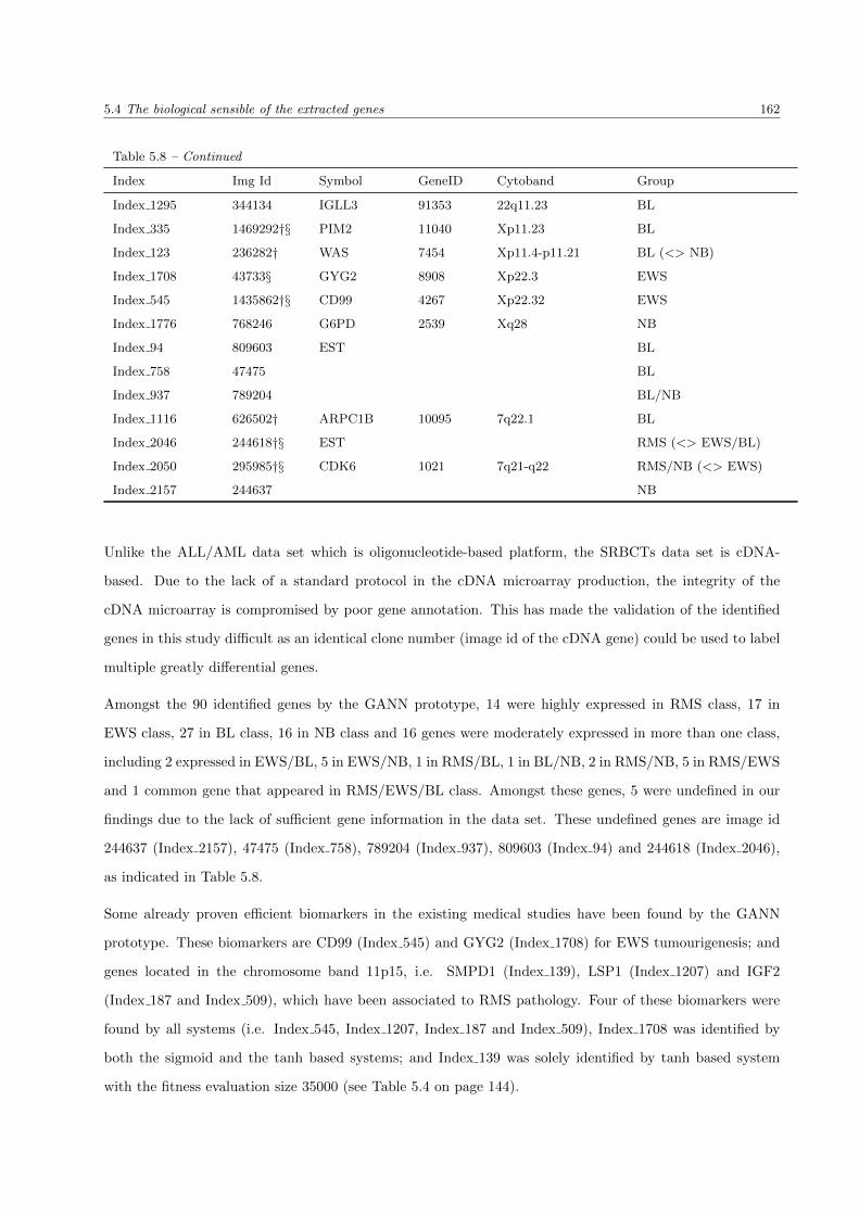
5.4 The biological sensible of the extracted genes 162
Table 5.8 – Continued
Index Img Id Symbol GeneID Cytoband Group
Index 1295 344134 IGLL3 91353 22q11.23 BL
Index 335 1469292†§ PIM2 11040 Xp11.23 BL
Index 123 236282† WAS 7454 Xp11.4-p11.21 BL (<> NB)
Index 1708 43733§ GYG2 8908 Xp22.3 EWS
Index 545 1435862†§ CD99 4267 Xp22.32 EWS
Index 1776 768246 G6PD 2539 Xq28 NB
Index 94 809603 EST BL
Index 758 47475 BL
Index 937 789204 BL/NB
Index 1116 626502† ARPC1B 10095 7q22.1 BL
Index 2046 244618†§ EST RMS (<> EWS/BL)
Index 2050 295985†§ CDK6 1021 7q21-q22 RMS/NB (<> EWS)
Index 2157 244637 NB
Unlike the ALL/AML data set which is oligonucleotide-based platform, the SRBCTs data set is cDNA-
based. Due to the lack of a standard protocol in the cDNA microarray production, the integrity of the
cDNA microarray is compromised by poor gene annotation. This has made the validation of the identified
genes in this study difficult as an identical clone number (image id of the cDNA gene) could be used to label
multiple greatly differential genes.
Amongst the 90 identified genes by the GANN prototype, 14 were highly expressed in RMS class, 17 in
EWS class, 27 in BL class, 16 in NB class and 16 genes were moderately expressed in more than one class,
including 2 expressed in EWS/BL, 5 in EWS/NB, 1 in RMS/BL, 1 in BL/NB, 2 in RMS/NB, 5 in RMS/EWS
and 1 common gene that appeared in RMS/EWS/BL class. Amongst these genes, 5 were undefined in our
findings due to the lack of sufficient gene information in the data set. These undefined genes are image id
244637 (Index 2157), 47475 (Index 758), 789204 (Index 937), 809603 (Index 94) and 244618 (Index 2046),
as indicated in Table 5.8.
Some already proven efficient biomarkers in the existing medical studies have been found by the GANN
prototype. These biomarkers are CD99 (Index 545) and GYG2 (Index 1708) for EWS tumourigenesis; and
genes located in the chromosome band 11p15, i.e. SMPD1 (Index 139), LSP1 (Index 1207) and IGF2
(Index 187 and Index 509), which have been associated to RMS pathology. Four of these biomarkers were
found by all systems (i.e. Index 545, Index 1207, Index 187 and Index 509), Index 1708 was identified by
both the sigmoid and the tanh based systems; and Index 139 was solely identified by tanh based system
with the fitness evaluation size 35000 (see Table 5.4 on page 144).

5.4 The biological sensible of the extracted genes 163
Figure 5.8: The heatmap of SRBCTs genes. The gene with high intensity (i.e. excited by the fluorescence dyes)denotes in red and the gene with low intensity denotes in blue.
The CD99 (MIC, Index 545) molecule is a very effective positive marker used to identify almost all EWS-
related patients and it can help to rule out any differential diagnostic considerations when used as part of
immunostaining techniques, i.e. antibody-based staining methods (Khoury, 2005). It was over-expressed in
almost all EWS samples in Figure 5.8 and presented in 2 RMS samples. It is also a useful marker to identify
lymphoblastic-related cancers including leukaemias and lymphomas (Kang and Dunphy, 2006). The gene
GYG2 (Index 1708) was moderately expressed in EWS class in Figure 5.8, but not in any of the tumour
classes in the data set which indicates that it is effectively more sensitive than CD99 in differentiating EWS
tumour from the other SRBCT-related groups.
Genes in chromosome band 11p15 have generated a particular interest in medical studies. This region accom-

5.4 The biological sensible of the extracted genes 164
modates various types of growth factor genes which play an important role in controlling the regulation of
various cellular processes in the body. Deregulation of the genes in this region is associated with over-growth
and tumour predisposition syndrome (Smith et al., 2007). Genes SMPD1 (Index 139), LSP1 (Index 1207)
and IGF2 (Index 187 and Index 509) were presented in RMS class in Figure 5.8 indicates that this region
may play a role in the pathogenesis of RMS. The gene IGF2 has been reported in the pathogenesis of RMS
by over-expression of the IGF2 level detected in ERMS subtype rather than in ARMS subtype (Makawita
et al., 2009).
In addition to biomarkers, some identified genes may also be involved in some known cytogenetic differenti-
ation among these four tumour groups. These genes are TNNT2 (Index 129) which may be associated with
MYOG and CD45 in EWS/RMS tumours; KIF3C (Index 1434) and may play a role in the ALK mutation
in NB tumour and LYN (Index 74) which may be associated with c-myc rearrangement in BL tumour.
The GANN prototype also identified some potential genes to be useful as biomarkers when used as a sole
differential diagnostic marker or as part of the immunostaining technique in detecting a specific tumour
group. These genes include ISG20 (Index 1387) in BL class; GAP43 (Index 1764) in NB class; SGCA
(Index 1003), MYL4 (Index 554) and FGFR4 (Index 1955) in RMS class; FGCRT (Index 1389), CAV1
(Index 246), TNFAIP6 (Index 566), PTPN13 (Index 1319) and KDSR (Index 1954) in EWS class; as is
indicated in Figure 5.8. There are also genes which were not expressed in certain tumour groups and these
genes may be useful in ruling rule out any differential tumour considerations in the diagnosis process.
SGCA (Index 1003) is the muscle specific protein that associated with muscular dystrophy and insulin-like
growth factor II (IGF2). High expression of SGCA in RMS class might be more indicative of the tissue origin
rather than related to the molecular background of RMS (Liden et al., 2002). While IGF2 gene (Index 187
and Index 509) is an already known oncogene associated with ERMS subtype cancer (Makawita et al., 2009).
FGFR4 (Index 1955) is a tyrosine kinase receptor that binds to fibroblast growth factor and to carry out the
signal transduction to the intracellular environment in cellular proliferation, differentiation and migration
(Pal et al., 2007). The activity of FGFR4 normally is undetectable (i.e. suppressed) in normal tissues,
however, it becomes active when a tumour is formed. High expression of FGFR4 in RMS tumour was
associated with advanced-stage cancer and poor survival (Taylor et al., 2009). In addition, over-expression
of FGFR4 has been shown in various cancers (Pal et al., 2007), i.e. pituitary, prostate and thyroid.
CAV1 (Index 246) is a putative tumour suppressor gene involved in the regulation of signal pathway. Low
expression of CAV1 has been associated to the development of colon cancer (Futschik et al., 2003). CAV1
has also been associated with prostate cancer (Liden et al., 2002). Mutation in CAV1 is usually a sign of
metastasis breast cancer (Bonuccelli et al., 2009).

5.5 The differentially expressed genes in various precision levels 165
The findings in this section showed that the GANN prototype able to identify genes that are not only related
to tumour histogenesis, but also genes that may not normally be expressed in the corresponding tissue. This
means that the GANN prototype does not detect genes exclusively associated with a single cancer type,
however, it explores genes that are differentially expressed in multiple cancer types. The identified genes
may provide new insights into the biology of the cancer. We also observed that the tanh based system
extracted more biological significant genes than the other systems.
5.5 The differentially expressed genes in various precision levels
In previous sections, we discussed the extraction performance of each system based on the implications from
two vital GA parameters that could affect the success of the system in extracting the most relevant genes
from the respective data set. The integrity of the findings have been discussed based on the expected results
from the synthetic data sets and the biology perspective.
In this section, the differentially expressed genes in three different fitness precision levels, i.e. 95%, 98% and
100% were examined. A comparison study based on these parameters was conducted using genes that were
overlapped in all four systems with a specific GA parameter condition, i.e. population size 300 and fitness
evaluation size 40000. Two tables, each representing a microarray data set, were produced. The complete
list of genes extracted by each system in different precision levels was listed in Tables B.13 and B.14 in
Appendix B. This design supports the objectives of our research theme stated in Section 1.4 on page 12.
Table 5.9: The summary list of overlapped ALL/AML genes with three different fitness precision levels.
Index Accession Number Symbol Precision Level
100% 98% 95%
Index 760 D88422 CSTA * * *
Index 804 HG1612-HT1612 MARCKSL1 * * *
Index 1685 M11722 DNTT * * *
Index 1779 M19507 MPO * * *
Index 1882 M27891 CST3 * * *
Index 2121 M63138 CTSD * * *
Index 2288 M84526 CFD * * *
Index 2354 M92287 CCND3 * * *
Index 2402 M96326 AZU1 * * *
Index 2642 U05259 CD79A * * *
Index 3252 U46499 MGST1 * * *
Index 4328 X59417 PSMA6 * * *
Index 4377 X62654 CD63 * * *
Continued on Next Page. . .

5.5 The differentially expressed genes in various precision levels 166
Table 5.9 – Continued
Index Accession Number Symbol Precision Level
100% 98% 95%
Index 4847 X95735 ZYX * * *
Index 6041 L09209 APLP2 * * *
Index 1829 M22960 CTSA * *
Index 6855 M31523 TCF3 * *
Index 1239 L07633 PSME1 * *
Index 1834 M23197 CD33 * *
Index 1928 M31303 STMN1 * *
Index 1962 M33680 CD81 * *
Index 4211 X51521 EZR * *
Index 5501 Z15115 TOP2B * *
Index 5772 U22376 MYB * *
Index 6200 M28130 IL8 * *
Index 6201 Y00787 IL8 * *
Index 6376 M83652 CFP * *
Index 4373 X62320 GRN * *
Index 412 D42043 RFTN1 *
Index 668 D86967 EDEM1 *
Index 1796 M20902 APOC1 *
Index 4196 X17042 SRGN *
Index 758 D88270 IGL@ *
Index 1745 M16038 LYN *
Table 5.9 shows the list of overlapped genes identified by all systems in the ALL/AML data set in three
different fitness precision levels, i.e. 100%, 98% and 95%. There were 30 common genes obtained in 100%
precision level, 31 common genes in 98% precision level and in 95% precision level, only 16 common genes
were found. Amongst these genes, 15 genes were expressed in all levels. These genes include some biomarkers,
i.e. DNTT, MPO and CD79A, that have been described in the previous section. The remaining genes were
only expressed when a specific precision level was applied. Twelve genes were detected in higher precision
levels, i.e. 98% and 100%, one gene (Index 4373) was found to be present in lower precision levels, i.e.
95% and 98%. These genes include CTSA (Index 1829), TCF3 (Index 6855), PSME1 (Index 1239), CD33
(Index 1834), STMN1 (Index 1928), CD81 (Index 1962), EZR (Index 4211), TOP2B (Index 5501), MYB
(Index 5772), IL8 (Index 6200 and Index 6201) and CFP (Index 6376) that were expressed in the precision
level 98% and above.
GRN (Index 4373)is a glycosylated peptide that has been cleaved into a variety of sections which may act
differently on cell growth. It is important in normal development of cell and brain, wound healing and

5.5 The differentially expressed genes in various precision levels 167
tumourigenesis. Mutation in GRN has been associated to brain disease, such as Alzheimer and dementia,
and has a crucial role in breast tumourigenesis (EntrezGene: GeneID 2896).
SRGN (Index 4196) encodes a haematopoietic cell granule proteoglycan protein, which was found to be
associated with the macromolecular complex of granzymes and perforin, which may serve as a mediator of
granule-mediated apoptosis (EntrezGene: GeneID 5552). LYN (Index 1745) is a tyrosine kinase that partic-
ipate in the regulation of cell activation. The expression of LYN has been associated to B-cell lymphocytes
(EntrezGene: GeneID 4067). SRGN, IGL@ (Index 758) and LYN have been identified with 98% fitness
precision level.
The findings showed that a low expression but biologically significant gene could be identified by the GANN
system. Although these lowly expressed genes are not directly associated in leukaemogenesis, however, they
play an important role in normal development and deficiency of these genes may lead to immunodeficiency
disease, which, in most cases, promotes tumourigenesis.
Table 5.10: The summary list of overlapped SRBCTs genes with three different fitness precision levels.
Index Image Id. Symbol Precision Level
100% 98% 95%
Index 1 21652 CTNNA1 * * *
Index 85 297392 MT1L * * *
Index 123 236282 WAS * * *
Index 187 296448 IGF2 * * *
Index 236 878280 CRMP1 * * *
Index 246 377461 CAV1 * * *
Index 255 325182 CDH2 * * *
Index 335 1469292 PIM2 * * *
Index 417 395708 DPYSL4 * * *
Index 509 207274 IGF2 * * *
Index 545 1435862 CD99 * * *
Index 554 461425 MYL4 * * *
Index 742 812105 MLLT11 * * *
Index 783 767183 HCLS1 * * *
Index 836 241412 ELF1 * * *
Index 846 183337 HLA-DMA * * *
Index 951 841620 DPYSL2 * * *
Index 976 786084 CBX1 * * *
Index 1003 796258 SGCA * * *
Index 1055 1409509 TNNT1 * * *
Index 1084 878652 PMS2L12 * * *
Continued on Next Page. . .

5.5 The differentially expressed genes in various precision levels 168
Table 5.10 – Continued
Index Image Id. Symbol Precision Level
100% 98% 95%
Index 1116 626502 * * *
Index 1158 814526 RBM38 * * *
Index 1207 143306 LSP1 * * *
Index 1319 866702 PTPN13 * * *
Index 1386 745019 EHD1 * * *
Index 1389 770394 FCGRT * * *
Index 1434 784257 KIF3C * * *
Index 1601 629896 MAP1B * * *
Index 1606 624360 PSMB8 * * *
Index 1645 52076 NOE1 * * *
Index 1916 80109 HLA-DQA1 * * *
Index 1954 814260 KDSR * * *
Index 1955 784224 FGFR4 * * *
Index 2046 244618 EST * * *
Index 2050 295985 CDK6 * * *
Index 153 383188 RCVRN * *
Index 1613 80338 SELENBP1 * *
Index 1327 491565 CITED2 * *
Index 1884 609663 PRKAR2B * *
Index 165 283315 PGAM2 *
Index 365 1473131 HOXB7 *
Index 107 365826 GAS1 *
For SRBCTs data set, as is indicated in Table 5.10, most of the identified genes, i.e. 36 genes, were presented
in all levels of fitness precision, including 1 undefined gene and some biomarkers, such as CD99, IGF2 and
LSP1. These genes may play a role as general markers for detecting small round undifferentiate cells.
Two genes (Index 153 and Index 1613) were detected in higher precision levels, i.e. 98% and 100%, but did
not appear in a lower precision level. Index 1327 and Index 1884 were found in both the highest (100%) and
the lowest (95%) precision levels, but not in 98%. This would indicate that these genes were provoked by
other abnormal genes. However, further molecular analysis on these genes should be performed to validate
their roles in tumourigenesis pathology.
Meanwhile, GAS1 (Index 107) was detected in 98% precision level. GAS1 is a putative tumor suppressor gene
involved in cell arrest and can induce apoptosis when it is over-expressed in different cell lines. It contains the
expected properties as a melanoma tumor suppressor: suppression of metastasis in a spontaneous metastasis
assay, promotion of apoptosis following dissemination of cells to secondary sites and down-regulation in

5.6 Raw microarray data set Versus Normalised microarray data set 169
human melanoma metastasis (EntrezGene: GeneID 2619).
To conclude, this section demonstrated the presence of differentially expressed genes in different precision
levels which could contribute to an early prognosis of tumourigenesis. The findings show the potential of
some genes which might be provoked by the presence of certain genes. This information could be useful for
therapeutic and biological diagnostic to prevent the development of tumour pathology.
5.6 Raw microarray data set Versus Normalised microarray data set
Referring to the problems stated in Section 1.2 on page 7, most of the oligonucleotide-based data sets were
generally preprocessed before being analysed by the computer algorithm. Table C.1 in Appendix C shows
some preprocessing techniques have been used in the ALL/AML data set. We argued that the quality of the
data set could be compromised by the normalisation process. To validate our statement, a comparison study
based on the raw and the normalised ALL/AML data sets was performed on each system in the population
size 300 and the fitness evaluation size 40000. A tailored C++ program is coded to scale down the gene
values to the [0, 1] interval, based on the maximum and the minimum values of a gene within the data set.
The equation of max-min normalisation is as follows:
xi =xi − xmin
xmax − xmin(5.1)
This max-min normalisation is being used in this study as it has been reported effective for the ensemble
ANN classifiers by Cho and Won (2007) in dealing the ALL/AML data set.
Table 5.11: The summary of the genes extracted from the raw and the normalised ALL/AML data sets.
System Raw data set Normaliseddata set
No. of consistentgenes
No. of selectedgenes solely pre-sented in the rawdata set
Sigmoid-based 45 86 35 10
Linear-based 55 92 47 8
Tanh-based 46 77 33 13
Threshold-based 47 94 41 6
Tables 5.11 and 5.12 present the summary of our findings and the complete list of the extracted genes is
presented in Table B.15 in Appendix B. The results show that by normalising the data set, the number of
genes identified by each system was tremendously increased. This is indicated by the increased number of

5.6 Raw microarray data set Versus Normalised microarray data set 170
Table 5.12: The processing time (in seconds) spent in the raw and the normalised ALL/AML data sets.
System Raw data set Normalised data set
Sigmoid based 8809 4007
Linear based 1951 1482
Tanh based 1644 6265
Threshold based 3036 1596
genes found in the normalised ALL/AML data set as compared to the genes identified in the raw ALL/AML
data set in Table 5.11. The normalisation process scaled down the magnitude of the gene values into a
specific interval, as a result, the highly differentially expressed genes were forced to be compressed to meet
the normalisation criteria and the significance of these genes was not obvious to the system. This is indicated
by a significant low selection frequency when similar genes were being selected in the normalised data set
as being selected in the raw data set (see Table B.15 in Appendix B). The chances to select low expression
but high biological relevant genes become impossible in the normalised data set as these genes have been
suppressed by other genes which have a higher expression values.
We observed a significant improvement in the processing time spent by the sigmoid, the linear and the
threshold based systems when the data set was normalised. However, the tanh based system required an
intensive processing time when analysing this normalised data set. This is because the tanh based system
adopting larger interval range, i.e. [-1, 1], in the selection process, whereas this normalised data set has a
smaller scaling range that is not appropriate for standard tanh computation.
The findings in this section has demonstrated the deficiency of using the normalisation process in the
ALL/AML data set, due to the quality of the data altered by the normalisation technique and, subsequently,
the integrity of the results was compromised.
We would like to draw the attention of researchers to the implication of normalisation techniques in the quality
of microarray data. The application of normalisation technique in the microarray data without understanding
the data itself could severely compromised the integrity of the results. This is due to microarray data being
much more complicated than the ordinary real-world data in the sense that it contains a multivariant of
cancer subtypes within a known cancer group and some of these cancer subtypes might associated with other
disease. Furthermore, the oligonucleotide microarray data are highly skewed with negative data values and
consequently, the biological relevant, however, lowly expressed genes in the data set may be ’buried’ by the
highly expressed ones in the data set. Therefore, the normalisation is usually expected in the oligonucleotide
microarray data to reduce the value skewness within the data. The improper use of normalisation techniques
could lead to an overly optimistic result and redundant information.
5.7 The significance of the extracted bioassay attributes 171
5.7 The significance of the extracted bioassay attributes
In the previous sections, we discussed the GANN performance to handle data with high feature dimension,
sample scarcity and complex feature interaction. Based on these findings, we observed that the tanh based
system is, amongst all the systems, the most effective system to extract the most significant features from
the biology perspective.
In this section, we examine the selection performance of the tanh based system to handle bioassay data
characterised by low feature dimension, feature-independent and highly imbalanced between the positive and
the negative samples. An experiment was conducted using the bioassay data sets based on the population
size 300 and the fitness evaluation size 30000. The completeness of the findings is evaluated using four
cost-sensitive classifiers constructed in the WEKA environment (see Section 4.1.2 on page 95 for parameter
settings) and is compared with the original work reported by Schierz (2009). The data sets have been split
into an 80% training set and a 20% test set, as recommended by Schierz. For AID362 data set, the training
set contains 3423 compounds, i.e. 48 active and 3375 inactive; and the test set contains 856 compounds, i.e.
12 active and 844 inactive. For AID688 data set, the training set has 21751 compounds, i.e. 198 active and
21553 inactive; and 5438 compounds, i.e. 50 active and 5388 inactive.
The top 20% of the attributes from each data set were selected by GANN prototype. To evaluate the
generalisation performance of the prototype, these selected attributes were trained by the identical set of
cost-sensitive classifiers (CSC) as reported in the original study (Schierz, 2009), i.e. Naive Bayes (CSC NB),
Support Vector Machine (CSC SMO), C4.5 tree (MetaCost J48) and Random Forest (CSC RF), with a 10-
fold cross-validation procedure. The significance of the attributes were then validated using the independent
test set.
Standard classifiers usually assume equal weighting of the classes in the data set, in the sense that mis-
classifying class A has similar consequences as misclassifying class B. As a result, most standard classifiers
are unable to predict a minority class in the bioassay data sets (Maloof, 2003; Schierz, 2009) due to highly
imbalanced data between active and inactive compounds in the data set. This led to the development of
cost-sensitive classifiers, which can assign different costing for different weighting classes in imbalanced data
sets (Domingos, 1999; Elkan, 2001; Maloof, 2003).
A trial experiment, based on the network size 10-5-2 using the AID362 data set was performed and the
results showed a poor performance on the system. This was due to the large data size of bioassay data
(4279-27189 samples) when compared to microarray data (72-83 samples), thus, we increased the network
size of GANN to 20-10-2, while the remaining parameters remain unchanged. Figure 5.9 shows the summary
of the results based on the independent test set of the data sets and the list of the selected attributes by
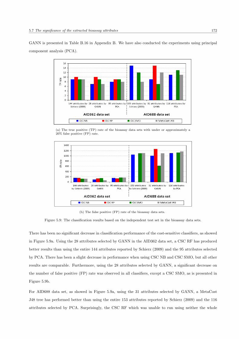
5.7 The significance of the extracted bioassay attributes 172
GANN is presented in Table B.16 in Appendix B. We have also conducted the experiments using principal
component analysis (PCA).
(a) The true positive (TP) rate of the bioassay data sets with under or approximately a20% false positive (FP) rate.
(b) The false positive (FP) rate of the bioassay data sets.
Figure 5.9: The classification results based on the independent test set in the bioassay data sets.
There has been no significant decrease in classification performance of the cost-sensitive classifiers, as showed
in Figure 5.9a. Using the 28 attributes selected by GANN in the AID362 data set, a CSC RF has produced
better results than using the entire 144 attributes reported by Schierz (2009) and the 95 attributes selected
by PCA. There has been a slight decrease in performance when using CSC NB and CSC SMO, but all other
results are comparable. Furthermore, using the 28 attributes selected by GANN, a significant decrease on
the number of false positive (FP) rate was observed in all classifiers, except a CSC SMO, as is presented in
Figure 5.9b.
For AID688 data set, as showed in Figure 5.9a, using the 31 attributes selected by GANN, a MetaCost
J48 tree has performed better than using the entire 153 attributes reported by Schierz (2009) and the 116
attributes selected by PCA. Surprisingly, the CSC RF which was unable to run using neither the whole

5.8 Summary 173
data set nor the 116 attributes selected by PCA, due to the size of the data set (∼ 27000 compounds),
has produced good results using the attributes selected by GANN. However, there has been a decrease in
performance using CSC NB and CSC SMO for attributes selected by GANN when compared to using the
entire attributes and the 116 attributes selected by PCA. Even so, all cost-sensitive classifiers have the lowest
FP using the 31 attributes selected by GANN (see Figure 5.9b).
The findings in this section demonstrate the efficiency of the GANN prototype to handle a large, imbalanced
data set. The results show a comparable better performance on the GANN prototype and the entire at-
tributes in the data set and the PCA. The advantage of using GANN to select attributes over using the entire
attributes and the PCA is that GANN enables computationally effective algorithms, such as Random Forest
and Classification Tree, to be implemented in a larger data set with a high success rate. Considering the
GANN prototype only implemented 20% of the attributes from the data set, the classification performance
of cost-sensitive classifiers has not been sacrificed. This shows that the GANN prototype has successfully
identified the most significant attributes needed to discriminate between the active and the inactive com-
pounds. The only downside of the GANN prototype is that a computationally intensive processing time
required for larger data set.
5.8 Summary
In this chapter, we examined the performance of the GANN model as a feature extraction. The prototype
was implemented to extract informative features (genes and attributes) from six data sets, comprising two
synthetic data, two microarray data and two bioassay data. The results can be summarised as follows:
• The linear based system is able to explore the potential genes more effectively than the other three sys-
tems and is very much processing cost effective as compared to the remaining three systems. However,
this system also induced a high number of low interest genes in the subject of study.
• The sigmoid based system is also able to efficiently explore the potential genes. However, this system
requires a more intensive processing cost than the other three systems.
• The threshold based system is lack of the stability factor in extracting consistent genes and it is sensitive
to data distribution.
• The tanh based system is, amongst the four systems, the most effective system to extract the most
informative genes from the data sets.
• All systems have a significant improvement on their performance with the population sizes 200 to 300
and the fitness evaluation sizes, ranging from 20000 to 40000.

5.8 Summary 174
• The identification of informative genes that were lower expressed in the data set can be achieved with
a low fitness precision level. These genes may be useful for therapeutic and biological diagnostic to
prevent the development of a tumour.
• The improper use of normalisation technique and a lack of understanding on the microarray data could
compromise the integrity of the results.
• The tanh based GANN system has produced better, or at least comparable, results in a large and imbal-
anced bioassay data set. However, the only downside of the GANN prototype is that a computationally
intensive processing time required for larger data set.
In the next chapter, we conclude our research by revising our contributions to the bioinformatics field, the
revision on our methodology and suggests the trend of the future research. The chapter will concluded with
the overall achievement of this thesis.

Chapter 6
Conclusion and Future Works
This chapter draws conclusions on our work reported in this thesis . A summary of the major contributions
of the research is provided and suggestions for possible further research areas.
This chapter contains five sections. Section 6.1 provides conclusions of the thesis. Section 6.2 summarises the
major contributions for this research. Section 6.3 presents the areas that have been omitted in this thesis.
Section 6.4 indicates the limitations of our research and suggests several interesting avenues for further work
to extend our research. Finally, Section 6.5 concludes the thesis with the overall achievements of the research.
6.1 Conclusions of the Thesis
This thesis presents an intelligent extraction approach via the hybridisation of GAs and ANNs to identify
informative features in the bioinformatics field. Our research emphasises the Ockham’s Razor principle to
extract features from high dimensional data and imbalanced data. Our approach is one of the very rare
feature extraction facilities that exploits the features of GAs and ANNs as a feature extraction and works
efficiently in two distinct types of data in the field. The main conclusions drawn from this thesis to answer
the research questions are given below.
1. Using the simplest parameter settings in both GA and ANN, primary features can be extracted from the
microarray data and these features show their biological significance on the tumourigenesis pathway.
2. The important genes which were lower expressed in the microarray data can be extracted with a lower
fitness precision level.
Some important conclusions derived from this the experimental study are given as below.
175

6.2 Summary of Contributions 176
1. The use of tanh activation function in ANNs, amongst four ANN functions, is the most effective
function to be used to compute the fitness function of a GA.
2. The GA has the best performance when the population size is between 200 to 300 and the fitness
evaluation sizes, ranging from 20000 to 40000.
3. The improper use of normalisation technique and a lack of understanding on the microarray data could
compromise the integrity of the gene selection results. This is because the normalisation technique
homogenised the magnitudes of the primary features with the secondary or the least significant features
in the data, and consequently, the chance of discovering primary features become narrowed.
6.2 Summary of Contributions
The main goal of this thesis was to devise a more effective way for extracting informative features from high
dimensional data using GAs and ANNs. This goal leads to three major contributions, which are reviewed
in related literature, the solution for feature extraction, the prototype implementation and evaluation. The
summary of these contributions is as follows:
6.2.1 The review of related literature
Two domains of literature pertaining to the biology and computer fields were reviewed. The existing biology
literature shows that there are two dominant types of microarrays: oligonucleotides and cDNA, each of which
requires different techniques to be used in the microarray production. The cDNA microarray usually requires
a two-phase in normalisation steps, i.e. the pre-normalisation in the fluorescent labelling process and the
post-normalisation in the imaging process. The oligonucleotide microarray requires only post-normalisation
in the imaging process. Both types of microarray data contain a high dimension of noisy genes, which require
the use of computer algorithm to analyse the data.
The existing computer literature shows that there are two dominant ways for analysing microarray data:
predicting the accuracy of the samples based on the known cancer group in the data; and discovering new
cancer groups from the known cancer group in the data. Both ways expose the immaturity of the gene
extraction area. Thus, in this thesis, we devised an efficient solution for extracting informative genes based
on the application of hybrid GAs and ANNs, as the previous research restricting the utility of the selection
method to retain the effectiveness of the classification method and the presentation of gene extraction based
upon the hybrid GA/ANN is rare. The rarity of this solution in feature extraction is mainly due to the
ill-conceived hypothesis in the existing works in dealing with microarray data. Another reason is because
both GAs and ANNs are not model transparent which lacks the step-by-step logic to explain the interaction

6.2 Summary of Contributions 177
between genes in the model. Thirdly, the ANN is commonly used as a classifier to classify samples and the
GA is usually used to optimise the parameter of the ANN. Promising results based on the incorporation of
GA into the ANN were reported in many discipline areas. Thus, researchers are not keen to find outcomes
when the ANN is incorporated into a GA.
Our work has incorporated the ANN into a GA using as minimal parameter setting as possible to avoid the
over-fitting problem which normally arises in ANNs. The ANN in our model is used as a fitness generator
to compute the GA fitness function.
The existing literature identifies several problems as follows:
• The lack of understanding of microarray data result in an ambiguity of the objectives of the study.
• The risk of over-fitting and biased underestimates of the error rate due to the misuse of a valid
mechanism and resusbstitution estimation in the classification process.
• The lack of supporting evidence in the declaration of new prediction models due to the misuse of a
valid mechanism and resusbstitution estimation.
• The researchers being not aware of the influence of the model complexity to the prediction results
which result in model over-fitting.
• The researchers being not aware of the influence of the data preprocessing in finding the relevant
information for the problems.
Information on these problems can be found in Sections 1.1 and 1.2 in Chapter 1 and Section 2.2 in Chapter
2.
6.2.2 The solution for feature extraction
Identifying a solution for feature extraction is the most important contribution of this research, as the
selection method is always needed to reduce the number of noisy information from microarray data. In our
solution, we utilised the universal computation power of ANNs and the evolutionary ability of GAs to extract
informative genes from a specific microarray data sets. Three main steps in our feature extraction model
are: (a) initialising a population of potential members to the problem, i.e. GA chromosomes; (b) computing
fitness values for each member in the population using a 3-layer feedforward ANN; and (c) evaluating the
fitness of each member in the population using GA crossover and mutation operators.
The capabilities of our solution are as follows:

6.2 Summary of Contributions 178
• The order of genes selected based on the selection frequency of genes, i.e. the number of times that the
gene is selected, and the fitness accuracy of the gene subset, i.e. the number of times that the sample
is correctly labelled in the class for the selected gene, is calculated.
• The fitness accuracy and the number of fitness evaluations for each GA cycle, i.e. GA generation, are
preserved.
• The flexibility to alter parameters, such as types of activation function to be used to compute fitness
values, the population size, the fitness evaluation size, the network size, the fitness precision level and
the gene list corresponds to a specific fitness accuracy to be displayed.
• The simplicity of the model in which only the fundamental parameter settings are applied which reduce
the possible risks arising from the complex model and also provides generalisability in handling multiple
types of data structures, i.e. microarray data and bioassay data, in the bioinformatics field.
• Retaining all highly fitted members for the next generation, excepting the least fit member which is
replaced by the new member in the next generation.
6.2.3 The prototype implementation and Evaluation
The prototype of the feature extraction solution has been implemented using a C++ programming language
in LINUX environment to realise the proposed techniques. This prototype helps to validate our approach and
shows the possibility of using ANN as a fitness generator for a GA, as well as extracting informative features
from the high dimensional data and in the highly imbalanced data with different data representations. The
prototype provided a fundamental basis for conducting our experimental study.
The performance of the prototype has been evaluated via experimental study which serve the following
purposes:
• The performance of prototype, each with a different ANN activation function, to extract informative
genes from the microarray data.
• The minimal sizes of GA population and fitness evaluation for efficient marker identification.
• The ability of prototype to handle different platform of microarray data.
• The ability of prototype to extract important genes that were lower expressed in microarray data set.
• The ability of prototype to handle a highly imbalanced data with multiple data representations.

6.3 Areas that are not explored in this thesis 179
6.3 Areas that are not explored in this thesis
There are several areas which were not explored in this thesis. These areas include:
• The mathematical proof on the logic of the activation function to calculate fitness values for each
member in the population.
• The implication of various data partition sizes in marker identification.
• The biological validation on the identified genes using RT-PCR assay or FISH analysis.
• The exploration in chemoinformatics literature and the challenges in the field.
• The exploration in pattern recognition literature for handling large and imbalanced data sets.
6.4 Limitations of this research and Further work
Our model has some limitations that should be improved in the future. These limitations are to handle data
with multiclasses more efficiently, to reproduce identical sets of extracted features and to reuse the selection
results.
• Although we have tested our model with two multiclass data sets in this thesis and the findings from
these data sets are promising, however, a lower fitness confidence level of the identified genes was
achieved compared to the fitness confidence level of the selected genes from the binary class data sets.
With the increased number of classes and different data representation, we may need to re-configure
the parameters in the model for better performance.
• Since our model did not preserve information of the network weights after each repetition run, the
reproduction of the identical set of genes is impossible, even though identical sets of parameter settings
were applied. With no preserved information of the network weights, we are unable to generate similar
fitness scores for the identical sets of chromosomes. When we consider the computational cost of our
model, with no preservation on the network weights used in the previous run, our model, in fact, has
a low computational cost as our model has less tasks to perform. Furthermore, each run represents a
new start on the GA and the ANN process in our model which can avoid the model being over-fitted
by prior information in the model.
• Our model produced only the list of identified genes ordered by its selection frequency and the total
number of correctly labelled samples after the completion of the maximum number of repetition runs.
As a result, the gene results cannot be reused in a different number of repetition runs.

6.5 The overall achievement of the thesis 180
For further work, we would like to explore the follows:
1. The implication of data partition on the significance of the extracted genes
One of the characteristics of microarray data is complex gene interactions, meaning that the number
of interacted genes are not fixed. Thus, by partitioning the data into different sizes and/or different
number of equal portions, different results may produced. Therefore, we would like to investigate the
potentiality of data partitioning in the effect of significant genes identified by our model.
2. Configurating the parameter of GANN
The current model using the fundamental configuration of the GA and the ANN. Although, promising
results are achieved, however, the level of fitness confidence for the selected genes from multiclass data
and data with different representation is low. This may be due to single-point crossover and binary
tournament selection being applied in our model. Thus, we would like to explore the potentiality of
different crossover operators and different variant of tournament selection techniques in improving the
fitness performance of the model in multiclass data and in imbalanced data.
3. Program new Functions
The existing model did not preserve the genes extracted in each repetition run. Thus, the selection
results cannot be reused when a different number of repetition runs is needed. In addition, the existing
model unable to associate the extracted genes to the respective class in the data set without the
assistance of an external tool. To circumvent the problem, we will write new program functions to
specifically preserve the list of genes extracted in each repetition run and to calculate the fitness
accuracy strength of the gene and, without increase the processing time in the current model.
4. Designing a User Interface
The current model has no proper user interface. All the changes of the parameter settings have to be
made directly in the C++ source code. This could increase the risk of logic errors that may be made
by the user which could yield undetected flaws in the results. Thus, we will program the window-based
interface in which the user can alter the parameter values and choose the report format to be displayed.
6.5 The overall achievement of the thesis
The overall achievement of this thesis can be summarised as follows:
• The first achievement is the presentation of a solution for extracting highly significant features from
high dimensional data sets.

6.5 The overall achievement of the thesis 181
• The second achievement is the way we hybrid GAs and ANNs which can utilised the minimal parameter
settings of the techniques to derive highly informative sets of genes.
• The third achievement is the experimental study conducted on four activation functions of ANNs in
different population size and GA evaluation, which has never been conducted before.
• The fourth achievement is the interpretation of the extracted genes from the biological perspectives
and its association to the disease of interest.
• The fifth achievement is the identification of the important genes appearing in different tumour devel-
opment stages and the precaution steps on these genes may prevent the spread and the growth of a
tumour.
• The sixth achievement is arguably novel, that is, our model is able to extract highly informative
features from multiple types of bioinformatics data, including microarray data that was characterised
with high gene dimension, sample scarcity and complex gene interaction; and bioassay data featured
with enormous compound size and highly imbalanced.
• Lastly, this thesis also demonstrate the practicality and the reliability of the solution through the
prototype.
Overall, we believe that our research makes advances in the feature extraction area in the bioinformat-
ics field. Our hybrid GANN method has proved that the selection on both the biological-relevant and
statistical-significant genes can be achieved using the raw, unprocessed microarray data. By deliberately not
emphasising on the quality of ANNs, true marker genes can be extracted by our model. Furthermore, our
approach also demonstrated its efficiency in dealing with bioassay data, which brings a new perspective in
finding the association between marker genes and pharmaceutical drug that is used to control the progression
of cancer disease. We believe that the findings presented in this thesis will draw more attention to the area
and stimulate more research in this field.

List of References
A.A. Alizadeh, M.B. Eisen, R.E. Davis, C. Ma, I.S. Lossos, A. Rosenwald, J.C. Boldrick, H. Sabet, T. Tran,
X. Yu, J.I. Powell, L. Yang, G.E. Marti, T. Moore, J.Jr. Hudson, L. Lu, D.B. Lewis, R. Tibshirani,
G. Sherlock, W.C. Chan, T.C. Greiner, D.D. Weisenburger, J.O. Armitage, R. Warnke, R. Levy, W. Wil-
son, M.R. Grever, J.C. Byrd, D. Botstein, P.O. Brown, and L.M. Staudt. Distinct types of diffuse large
B-cell lymphoma identified by gene expression profiling. Nature, 403:503–511, 2000.
C. Ambroise and G.J. McLachlan. Selection bias in gene extraction on the basis of microarray gene-expression
data. PNAS, 99(10):6562–6566, 2002.
I.P. Androulakis. Selecting maximally informative genes. Computers and Chemical Engineering, 29(3):
535–546, 2005.
D.A. Arber, D.S. Snyder, M. Fine, A. Dagis, J. Niland, and M.L. Slovak. Myeloperoxidase immunoreactivity
in adult acute lymphoblastic leukemia. Am J Clin Pathol, 116(1):25–33, 2001.
J. Arifovic and R. Gencay. Using genetic algorithms to select architecture of a feedforward artificial neural
network. Physica A, 289(3):574–594, 2001.
S.A. Armstrong, J.E. Staunton, L.B. Silverman, R. Pieters, M.L. den Boer, M.D. Minden, S.E. Sallan, E.S.
Lander, T.R. Golub, and S.J. Korsmeyer. MLL translocations specify a distinct gene expression profile
that distinguishes a unique leukemia. Nature Genetics, 30(1):41–47, 2002.
M.H. Asyali, D. Colak, O. Demirkaya, and M.S. Inan. Gene expression profile classification: A review.
Current Bioinformatics, 1:55–73, 2006.
R.P. Auburn, D.P. Kreil, L.A. Meadows, B. Fischer, S.S. Matilla, and S. Russell. Robotic spotting of cDNA
and oligonucleotide microarrays. Trends Biotechnology, 23(7):374–379, 2005.
M. Barletta, A. Gisario, and S. Guarino. Modelling of electrostatic fluidized bed (EFB) coating process
using artificial neural networks. Eng. Appl. Artif. Intell., 20(6):721–733, 2007.
182

LIST OF REFERENCES 183
D. Beasley, D.R. Bull, and R.R. Martin. An overview of genetic algorithms: Part I, fundamentals. University
Computing, 15(2):58–69, 1993.
R.G. Beiko and R.L. Charlebois. GANN: Genetic algorithm neural networks for the detection of conserved
combinations of features in DNA. BMC Bioinformatics, 6(36), 2005.
M. Bernsteina, H. Kovarb, M. Paulussenc, R. Lor Randalld, A. Schucke, L.A. Teotf, and H. Juergensgg.
Ewings sarcoma family of tumors: Current management. The Oncologist, 11(5):503–519, 2006.
V. Bevilacqua, G. Mastronardi, and F. Menolascina. Genetic algorithm and neural network based classifica-
tion in microarray data analysis with biological validity assessment. In D-S Huang, K.L, and G.W. Irwin,
editors, ICIC’06: Computational Intelligence and Bioinformatics, International Conference on Intelligent
Computing, proceedings, Part III, volume 4115 of Lecture Notes in Computer Science, pages 475–484.
Springer, 2006a.
V. Bevilacqua, G. Mastronardi, F. Menolascina, A. Paradiso, and S. Tommasi. Genetic algorithms and
artificial neural networks in microarray data analysis: a distributed approach. Engineering Letters -
Special Issue on Bioinformatics, 13(3):335–343, 2006b.
G. Bloom, I.V. Yang, D. Boulware, K.Y. Kwong, D. Coppola, S. Eschrich, J. Quackenbush, and T.J. Yeat-
man. Multi-platform, multi-site, microarray-based human tumor classification. American Journal of
Pathology, 164(1):9–16, 2004.
T.H. Bø and I. Jonassen. New feature subset selection procedures for classification of expression profiles.
Genome Biology, 3(4):research00, 2002.
G. Bonuccelli, M.C. Casimiro, F. Sotgia, C. Wang, M. Liu, S. Katiyar, J. Zhou, E. Dew, F. Capozza, K.M.
Daumer, C. Minetti, J.N. Milliman, F. Alpy, M.C. Rio, C. Tomasetto, I. Mercier, N. Flomenberg, P.G.
Frank, R.G. Pestell, and M.P. Lisanti. Caveolin-1 (p132l), a common breast cancer mutation, confers
mammary cell invasiveness and defines a novel stem cell/metastasis-associated gene signature. Am J
Pathol., 174(5):1650–1662, 2009.
A.L. Boulesteix, C. Strobl, T. Augustin, and M. Daumer. Evaluating microarray-based classifiers: An
overview. Cancer Informatics, 6:77–97, 2008.
S. Brenner, M. Johnson, J. Bridgham, G. Golda, D.H. Lloyd, D. Johnson, S. Luo, S. McCurdy, M. Foy,
M. Ewan, R. Roth, D. George, S. Eletr, G. Albrecht, E. Vermaas, S.R. Williams, K. Moon, T. Burcham,
M. Pallas, R.B. DuBridge, J. Kirchner, K. Fearon, J i. Mao, and K. Corcoran. Gene expression analysis
by massively parallel signature sequencing (MPSS) on microbead arrays. Nature Biotechnology, 18(6):
630–634, 2000.

LIST OF REFERENCES 184
N. Brown. Chemoinformatics—an introduction for computer scientists. ACM Computing Surveys, 41(2):
1–38, 2009.
H. Bruchova, M. Kalinova, and R. Brdicka. Array-based analysis of gene expression in childhood acute
lymphoblastic leukemia. Leukemia Research, 28:1–7, 2004.
F. Busetti. Genetic algorithms overview. Available from: http://citeseer.nj.nec.com/464346.html [Accessed
31 October 2007], 2001.
H. Cartwright. Using artificial intelligence in chemistry and biology: A practical guide, chapter Artificial
Neural Networks, pages 9–49. CRC Press, Taylor & Francis Group, 2008a.
H. Cartwright. Using artificial intelligence in chemistry and biology: A practical guide, chapter Evolutionary
Algorithms, pages 113–172. CRC Press, Taylor & Francis Group, 2008b.
Q-R. Chen, G. Vansant, K. Oades, M. Pickering, J.S. Wei, Y.K. Song, J. Monforte, and J. Khan. Diagnosis
of the small round blue cell tumors using multiplex polymerase chain reaction. Journal of Molecular
Diagnostics, 9(1):80–88, 2007.
Y.H. Chen, Y.M. Tang, H.Q. Shen, H. Song, S.L. Yang, S.W. Shi, B.Q. Qian, W.Q. Xu, and B.T. Ning.
The expression of CD19 in 210 cases of childhood acute leukemia and its significance. Zhonghua Er Ke
Za Zhi, 42(3):188–191, 2004.
J. Cheng and Q.S. Li. Reliability analysis of structures using artificial neural network based genetic algo-
rithms. Comput. Methods Appl. Mech. Engrg., 197(45-48):3742–3750, 2008.
M-Y. Cheng and C-H. Ko. A genetic-fuzzy-neuro model encodes FNNs using SWRM and BRM. Engineering
Applications of Artificial Intelligence, 19(8):891–903, 2006.
G. Chetty and M. Chetty. Multiclass microarray gene expression analysis based on mutual dependency
models. In V. Kadirkamanathan et al., editor, PRIB’09: 4th IAPR International Conference on Pattern
Recognition in Bioinformatics, proceedings, volume 5780 of Lecture Notes in Bioinformatics, pages 46–55,
2009.
H.S. Cho, T.S. Kim, J.W. Wee, S.M. Jeon, and C.H Lee. cDNA microarray data based classification of
cancers using neural networks and genetic algorithms. In Nanotech’03: Nanotechnology Conference and
Trade Show, proceedings, volume 1, 2003a.
J-H. Cho, D. Lee, J.H. Park, and I-B. Lee. New gene selection method for classification of cancer subtypes
considering within-class variation. FEBS letters, 551(1-3):3–7, 2003b.

LIST OF REFERENCES 185
S-B. Cho and H-H. Won. Machine learning in dna microarray analysis for cancer classification. In Y-
P.P. Chen, editor, APBC’03: P1st Asia-Pacific bioinformatics conference on Bioinformatics, proceedings,
volume 19, pages 189–198. Australian Computer Society, 2003.
S.B. Cho and H-H. Won. Cancer classification using ensemble of neural networks with multiple significant
gene subsets. Applied Intelligence, 26(3):243–250, 2007.
W. Chu, Z. Ghahramani, F. Falciani, and D.L. Wild. Biomarker discovery in microarray gene expression
data with gaussian processes. Bioinformatics, 21(16):3385–3393, 2005.
J.A. Cruz and D.S. Wishart. Applications of machine learning in cancer prediction and prognosis. Cancer
Informatics, 2:59–78, 2006.
A.C. Culhane, G. Perriere, E.C. Considine, T.G. Cotter, and D.G. Higgins. Between-group analysis for
microarray data. Bioinformatics, 18(12):1600–1608, 2002.
A.R. Dabney. Classification of microarrays to nearest centroids. Bioinformatics, 21(22):4148–4154, 2005.
H.K. Dadi, A.J. Simon, and C.M. Roifman. Effect of CD3delta deficiency on maturation of alpha/beta
and gamma/delta t-cell lineages in severe combined immunodeficiency. N Engl J Med, 349(19):1821–1828,
2003.
K.A. DeJong. Learning with genetic algorithms: An overview. Machine Learning, 3(2-3):121–138, 1988.
K.A. DeJong and W.M. Spears. An analysis of the interacting roles of population size and crossover in genetic
algorithms. In H-P. Schwefel and R. Manner, editors, PPSN’91: 1st Workshop on Parallel Problem Solving
from Nature, proceedings, volume 496 of Lecture Notes in Computer Science, pages 38–47. Springer, 1991.
J.M. Deutsch. Algorithm for finding optimal gene sets in microarray prediction. Available from:
http://stravinsky.ucsc.edu/josh/gesses, August 2001. [Accessed 31 October 2007].
J.M. Deutsch. Evolutionary algorithms for finding optimal gene sets in microarray prediction. Bioinformatics,
19(1):45–52, 2003.
R. Dıaz-Uriarte and S.A. de Andres. Gene selection and classification of microarray data using random
forest. BMC Bioinformatics, 7:3, 2006.
B. Djavan, M. Remzi, A. Zlotta, C. Seitz, P. Snow, and M. Marberger. Novel artificial neural network for
early detection of prostate cancer. J Clin Oncol., 20(4):921–929, 2002.
P. Domingos. Metacost: a general method for making classifiers cost-sensitive. In KDD’99: Fifth ACM
SIGKDD international conference on Knowledge discovery and data mining, proceedings, pages 155–164,
1999.

LIST OF REFERENCES 186
S. Dudoit, J. Fridlyand, and T.P. Speed. Comparison of discrimination methods for the classification of
tumors using gene expression data. Technical report 576, Department of Statistics, University of California,
Berkeley, June 2000.
S. Dudoit, J. Fridlyand, and T.P. Speed. Comparison of discrimination methods for the classification of
tumors using gene expression data. Journal of the American Statistical Association, 97(457):77–87, 2002.
A. Dupuy and R.M. Simon. Critical review of published microarray studies for cancer outcome and guidelines
on statistical analysis and reporting. JNCI Journal of the National Cancer Institute, 99(2):147–157, 2007.
R. Dybowski, P. Weller, R. Chang, and V. Gant. Prediction of outcome in critically ill patients using artificial
neural network synthesised by genetic algorithm. THE LANCET, 347(9009):1146–1150, 1996.
B.L. Ebert and T.R. Golub. Genomic approaches to hematologic malignancies. Blood, 104(4):923–932, 2004.
C. Elkan. The foundations of cost-sensitive learning. In IJCAI’01: Seventeenth International Joint Confer-
ence on Artificial Intelligence, proceedings, pages 973–978, 2001.
M.H. Fatemi. Prediction of ozone tropospheric degradation rate constant of organic compounds by using
artificial neural networks. Analytica Chimica Acta, 556(2):355–363, 2006.
T. Froese, S. Hadjiloucas, R.K.H. Galv ao, V.M. Becerra, and C.J. Coelho. Comparison of extrasystolic ecg
signal classifiers using discrete wavelet transforms. Pattern Recogn. Lett., 27(5):393–407, 2006.
M.E. Futschik, A. Reeve, and N. Kasabov. Evolving connectionist systems for knowledge discovery from
gene expression data of cancer tissue. Artificial Intelligence in Medicine, 28:165–189, 2003.
J. Gasteiger. Chemoinformatics: a new field with a long tradition. Analytical and Bioanalytical Chemistry,
384(1):57–64, 2006.
D.E. Goldberg. Genetic Algorithms in Search, Optimization & Machine Learning, chapter Some Applications
of Genetic Algorithms, pages 59–88. Addison Wesley Longman, 1989.
D.E. Goldberg and K. Deb. A comparative analysis of selection schemes used in genetic algorithms. In G.J.E.
Rawlins, editor, FOGA’90: 1st Workshop on Foundations of Genetic Algorithms, proceedings, pages 69–93.
Morgan Kaufmann, 1990.
T.R. Golub, D.K. Slonim, P. Tamayo, C. Huard, M. Gaasenbeek, J.P. Mesirov, H. Coller, M.L. Loh, J.R.
Downing, M.A. Caligiuri, C.D. Bloomfield, and E.S. Lander. Molecular classification of cancer: Class
discovery and class prediction by gene expression monitoring. Science, 286(5439):531–536, 1999.

LIST OF REFERENCES 187
S.M. Gonia, S. Oddone, J.A. Segura, R.H. Mascheroni, and V.O. Salvadori. Prediction of foods freezing and
thawing times: Artificial neural networks and genetic algorithm approach. Journal of Food Engineering,
84(1):164–178, 2008.
Z. Guan and H. Zhao. A semiparametric approach for marker gene selection based on gene expression data.
Bioinformatics, 21(4):529–536, 2005.
I. Guyon and A. Elisseeff. An introduction to variable and feature selection. J. Mach. Learn. Res., 3:
1157–1182, 2003.
I. Guyon, J. Weston, S. Barnhill, and V. Vapnik. Gene selection for cancer classification using support vector
machines. Machine Learning, 46(1-3):389–422, 2002.
M. Hall, E. Frank, G. Holmes, B. Pfahringer, P. Reutemann, and I.H. Witten. The WEKA data mining
software: An update. volume 11, 2009.
C. Hayter. Cancer: “the worst scourge of civilized mankind”. Can Bull Med Hist., 20(2):251–264, 2003.
G. He, D. Wu, A. Sun, Y. Xue, Z. Jin, H. Qiu, M. Miao, X. Tang, Z. Fu, and Z. Chen. Cyt CD79a expression
in acute leukemia with t(8;21): biphenotypic or myeloid leukemia? Cancer Genet Cytogenet, 174(1):76–77,
2007.
P.S. Heckerling, G.J. Canaris, S.D. Flach, T.G. Tape, R.S. Wigton, and B.S. Gerber. Predictors of urinary
tract infection based on artificial neural networks and genetic algorithms. International Journal of Medical
Informatics, 76(4):289–296, 2007.
J.H. Holland. Adaptation in Natural and Artificial Systems. The MIT Press, 1992. ISBN 0-262-08213-6.
K.K. Hoyer, M. Herling, K. Bagrintseva, D.W. Dawson, S.W. French, M. Renard, J.G. Weinger, D. Jones,
and M.A. Teitell. T cell leukemia-1 modulates TCR signal strength and IFN-gamma levels through
phosphatidylinositol 3-kinase and protein kinase c pathway activation. J Immunol, 175(2):864–873, 2005.
HQ.P. Hu, M. Xie, S.H. Ng, and G. Levitin. Robust recurrent neural network modeling for software fault
detection and correction prediction. Reliability Engineering & System Safety, 92(3):332–340, 2007.
K.B. Hwang, D.Y. Cho, S.W. Park, S.D. Kim, and B.Y. Zhang. Applying machine learning techniques to
analysis of gene expression data: Cancer diagnosis. In CAMDA’02: The Conference on Critical Assessment
of Microarray Data Analysis, proceedings, pages 167–182, 2002.
I. Inza, P. Larranaga, R. Blanco, and A.J. Cerrolaza. Filter versus wrapper gene selection approaches in
DNA microarray domains. Artificial Intelligence in Medicine, 31(2):91–103, 2004.

LIST OF REFERENCES 188
I.B. Jeffery, D.G. Higgins, and A.C. Culhane. Comparison and evaluation of methods for generating differ-
entially expressed gene lists from microarray data. BMC Bioinformatics, 7:359, 2006.
I.S. Jeon, J.N. Davis, B.S. Braun, J.E. Sublett, M.F. Roussel, C.T. Denny, and D.N. Shapiro. A variant
ewing’s sarcoma translocation (7;22) fuses the EWS gene to the ETS gene ETV1. Oncogene, 10(6):
1229–1234, 1995.
D. Jiang, C. Tang, and A. Zhang. Cluster analysis for gene expression data: A survey. IEEE Transaction
on Knowledge and Data Engineering, 16(11):1370–1386, 2004.
T. Jirapech-Umpai and S. Aitken. Feature selection and classification for microarray data analysis: Evolu-
tionary methods for identifying predictive genes. BMC Bioinformatics, 6:148, 2005.
L.C. Kang and C.H. Dunphy. Immunoreactivity of MIC2 (CD99) and terminal deoxynucleotidyl transferase
in bone marrow clot and core specimens of acute myeloid leukemias and myelodysplastic syndromes. Arch
Pathol Lab Med, 130(2):153–157, 2006.
M. Karzynski, A. Mateos, J. Herrero, and J. Dopazo. Using a genetic algorithm and a perceptron for feature
selection and supervised class learningin DNA microarray data. Artif. Intell. Rev., 20(1-2):39–51, 2003.
E.C. Keedwell and A. Narayanan. Genetic algorithms for gene expression analysis. In Raidl et al., editor,
EvoWorkshops’03: Applications in Evolutionary Computing, 1st European Workshop on Evolutionary
Bioinformatics, proceedings, volume 2611 of Lecture Notes in Computer Science, pages 76–86. Springer,
2003.
T.W. Kelley, D. Huntsman, K.M. McNagny, C.D. Roskelley, and E.D. Hsi. Podocalyxin: a marker of blasts
in acute leukemia. Am J Clin Pathol, 124(1):134–142, 2005.
J. Khan, J.S. Wei, M. Ringner, L.H. Saal, M. Ladanyi, F. Westermann, F. Berthold, M. Schwab, C.R.
Antonescu, C. Peterson, and P.S. Meltzer. Classification and diagnostic prediction of cancers using gene
expression profiling and artificial neural networks. Nature Medicine, 7:673–679, 2001.
H. Khoury, B.I. Dalal, S.H. Nantel, D.E. Horsman, J.C. Lavoie, J.D. Shepherd, D.E. Hogge, C.L. Toze, K.W.
Song, D.L. Forrest, H.J. Sutherland, and T.J. Nevill. Correlation between karyotype and quantitative
immunophenotype in acute myelogenous leukemia with t(8;21). Mod Pathol, 17(10):1211–1216, 2004.
J.D. Khoury. Ewing sarcoma family of tumors. Adv Anat Pathol, 12(4):212–220, 2005.
H. Kim, G.H. Golub, and H. Park. Missing value estimation for DNA microarray gene expression data:
local least squares imputation. Bioinformatics, 21(2):187–198, 2005.

LIST OF REFERENCES 189
K-J. Kim and I. Han. Genetic algorithms approach to feature discretization in artificial neural networks for
the prediction of stock price index. Expert Systems with Applications, 19(2):125–132, 2000.
B. Kisacik, A. Akdogan, G. Yilmaz, O. Karadag, F.M. Yilmaz, S. Koklu, O. Yuksel, A.I. Ertenli, and
S. Kiraz. Serum adenosine deaminase activities during acute attacks and attack-free periods of familial
mediterranean fever. Eur J Intern Med, 20(1):44–47, 2009.
N. Kiyokawa, T. Sekino, T. Matsui, H. Takenouchi, K. Mimori, W.R. Tang, J. Matsui, T. Taguchi, Y.U.
Katagiri, H. Okita, Y. Matsuo, H. Karasuyama, and J. Fujimoto. Diagnostic importance of CD179a/b as
markers of precursor b-cell lymphoblastic lymphoma. Mod Pathol, 17(4):423–429, 2004.
D. Ko, W. Xu, and B. Windle. Gene function classification using NCI-60 cell line gene expression profiles.
Computational Biology and Chemistry, 29(6):412–419, 2005.
R. Kohavi and G.H. John. Wrappers for feature subset selection. Artif. Intell., 97(1-2):273–324, 1997.
S.B. Kotsiantis. Supervised machine learning: A review of classification. Informatica, 31:249–268, 2007.
S.B. Kotsiantis, D. Kanellopoulos, and P.E. Pintelas. Data preprocessing for supervised leaning. International
Journal of Computer Science, 1(2):111–117, 2006.
W.P. Kuo, E-Y. Kim, J. Trimarchi, T-K. Jenssen, S.A. Vinterbo, and L. Ohno-Machado. A primer on gene
expression and microarrays for machine learning researchers. J. of Biomedical Informatics, 37(4):293–303,
2004.
Y-K. Kwon and B.R. Moon. Nonlinear feature extraction using a neuro genetic hybrid. In H-G. Beyer
and U-M. O‘Reilly, editors, GECCO’05: Genetic and Evolutionary Computation Conference, proceedings,
pages 2089–2096, New York, NY, USA, 2005. ACM.
D. Lee, J.W. Kim, T. Seoand S.G. Hwang, E.J. Choi, and J. Choe. SWI/SNF complex interacts with tumor
suppressor p53 and is necessary for the activation of p53-mediated transcription. J Biol Chem, 277(25):
22330–22337, 2002.
J.W. Lee, J.B. Lee, M. Park, and S.H. Song. An extensive comparison of recent classification tools applied
to microarray data. Computational statistics & data analysis, 48(4):869–885, 2005.
Y. Lee and C-K. Lee. Classification of multiple cancer types by multicategory support vector machines using
gene expression data. Bioinformatics, 19(9):1132–1139, 2003.
Y.F. Leung and D. Cavalieri. Fundamentals of cDNA microarray data analysis. Trends in Genetics, 19(11):
649–659, 2003.

LIST OF REFERENCES 190
L. Li, T.A. Darden, C.R. Weinberg, A.J. Levine, and L.G. Pedersen. Gene assessment and sample clas-
sification for gene expression data using a genetic algorithm/k-nearest neighbor method. Combinatorial
Chemistry & High Throughput Screen, 4:727–739, 2001a.
L. Li, C.R. Weinberg, T.A. Darden, and L.G. Pedersen. Gene selection for sample classification based on gene
expression data: Study of sensitivity to choice of parameters of the GA/kNN method. Bioinformatics, 17
(12):1131–1142, 2001b.
T. Li, C. Zhang, and M. Ogihara. A comparative study of feature selection and multiclass classification
methods for tissue classification based on gene expression. Bioinformatics, 20(15):2429–2437, 2004.
W. Li and Y. Yang. How many genes are needed for a discriminant microarray data analysis? In S.M.
Lin and K.F. Johnson, editors, Methods of Microarray Data Analysis, CAMDA’00: Critical Assessment of
Techniques for Microarray Data Analysis, pages 137–150. Kluwer Academic, 2002.
P. Liden, L. Asker, and H. Bostrom. Rule induction for classification of gene expression array data. In
PKDD’02: 6th European Conference on Principles of Data Mining and Knowledge Discovery, proceedings,
pages 338–347. Springer, 2002.
T-C. Lin, R-S. Liu, Y-T. Chao, and S-Y. Chen. Multiclass microarray data classification using GA/ANN
method. In Q. Yang and G.I. Webb, editors, PRICAI’06: Trends in Artificial Intelligence, 9th Pacific Rim
International Conference on Artificial Intelligence, proceedings, volume 4099 of Lecture Notes in Computer
Science, pages 1037–1041. Springer, 2006.
B. Liu, Q. Cui, T. Jiang, and S. Ma. A combinational feature selection and ensemble neural network method
for classification of gene expression data. BMC Bioinformatics, 5:136, 2004a.
J.J. Liu, G. Cutler, W. Li, Z. Pan, S. Peng, T. Hoey, L. Chen, and X.B. Ling. Multiclass cancer classification
and biomarker discovery using GA-based algorithms. Bioinformatics, 21(11):2691–2697, 2005a.
L. Liu, L. McGavran, M.A. Lovell, Q. Wei, B.A. Jamieson, S.A. Williams, N.N. Dirks, M.S. Danielson,
L.M. Dubie, and X. Liang. Nonpositive terminal deoxynucleotidyl transferase in pediatric precursor b-
lymphoblastic leukemia. Am J Clin Pathol, 121(6):810–815, 2004b.
X. Liu, A. Krishnan, and A. Mondry. An entropy-based gene selection method for cancer classification using
microarray data. BMC Bioinformatics, 6:76, 2005b.
Z. Liu, C. Wang, A. Liu, and Z. Niu. Evolving neural network using real coded genetic algorithm (GA) for
multispectral image classification. Future Generation Computer Systems, 20(7):1119–1129, 2004c.

LIST OF REFERENCES 191
Y. Lu and J. Han. Cancer classification using gene expression data. Information Systems, 28(4):243–268,
2003.
N. Mah, A. Thelin, T. Lu, S. Nikolaus, T. Kuhbacher, Y. Gurbuz, H. Eickhoff, G. Kloppel, H. Lehrach,
B. Mellgard, C.M. Costello1, and S. Schreiber. A comparison of oligonucleotide and cDNA-based microar-
ray systems. Physiol. Genomics, 16:361–370, 2004.
S. Makawita, M. Ho, A.D. Durbin, P.S. Thorner, D. Malkin, and G.R. Somers. Expression of insulin-like
growth factor pathway proteins in rhabdomyosarcoma: IGF-2 expression is associated with translocation-
negative tumors. Pediatr Dev Pathol, 12(2):127–135, 2009.
M. Maloof. Learning when data sets are imbalanced and when costs are unequal and unknown. In ICML’03:
Workshop on Learning from Imbalanced Data Sets, proceedings, 2003.
Y. Mao, X. Zhou, D. Pi, Y. Sun, and S.T.C. Wong. Multiclass cancer classification by using fuzzy support
vector machine and binary decision tree with gene selection. Journal of Biomedicine and Biotechnology,
2005(2):160–171, 2005.
F. Markowetz and R. Spang. Molecular diagnosis: Classification, model selection and performance evaluation.
Methods Inf Med., 44(3):438–443, 2005.
P.P. Medina, O.A. Romero, T. Kohno, L.M. Montuenga, R. Pio, J. Yokota, and M. Sanchez-Cespedes.
Frequent BRG1/SMARCA4-inactivating mutations in human lung cancer cell lines. Hum Mutat, 29(5):
617–622, 2008.
T.M. Mitchell. Machine Learning. McGraw-Hill, 1997a.
T.M. Mitchell. Does machine learning really work? AI Magazine, 18(3):11–20, 1997b.
S. Mocellin and C.R. Rossi. Principles of gene microarray data analysis. Advances in experimental medicine
and biology, 593:19–30, 2007.
D.J. Montana and L. Davis. Training feedforward neural networks using genetic algorithms. In 11th In-
ternational Joint Conference on Artificial Intelligence, proceedings, pages 762–767. Morgan Kaufmann,
1989.
Y.P. Mosse, M. Laudenslager, L. Longo, K.A. Cole, A. Wood, E.F. Attiyeh, M.J. Laquaglia, R. Sennett, J.E.
Lynch, P. Perri, G. Laureys, F. Speleman, C. Kim, C. Hou, H. Hakonarson, A. Torkamani, N.J. Schork,
G.M. Brodeur, G.P. Tonini, E. Rappaport, M. Devoto, and J.M. Maris. Identification of ALK as a major
familial neuroblastoma predisposition gene. Nature, 455(7215):930–935, 2008.

LIST OF REFERENCES 192
M. Mramor, G. Leban, J. Demsar, and B. Zupan. Conquering the curse of dimensionality in gene expression
cancer diagnosis: Tough problem, simple models. In S. Miksch, J. Hunter, and E.T. Keravnou, editors,
AIME’05: 10th Conference on Artificial Intelligence in Medicine, proceedings, volume 3581 of Lecture
Notes in Computer Science, pages 514–523. Springer, 2005.
C.G. Mullighan, S. Goorha, I. Radtke, C.B. Miller, E. Coustan-Smith, J.D. Dalton, K. Girtman, S. Mathew,
J. Ma, S.B. Pounds, X. Su, C-H. Pui, M.V. Relling, W.E. Evans, S.A. Shurtleff, and J.R. Downing.
Genome-wide analysis of genetic alterations in acute lymphoblastic leukaemia. Nature, 446:758–764, 2007.
L. Nanni and A. Lumini. Ensemblator: An ensemble of classifiers for reliable classification of biological data.
Pattern Recognition Letters, 28(5):622–630, 2007.
A. Narayanan, A. Cheung, J. Gamalielsson, E. Keedwell, and C. Vercellone. Bioinformatics using Com-
putational Intelligence Paradigms, chapter Artificial Neural Networks for Reducing the Dimensionality of
Gene Expression Data. Studies in Fuzziness and Soft Computing. Springer Berlin / Heidelberg, 2005.
M. Nasseri, K. Asghari, and M.J. Abedini. Optimized scenario for rainfall forecasting using genetic algorithm
coupled with artificial neural network. Expert Syst. Appl., 35(3):1415–1421, 2008.
G. Nunnari. Modelling air pollution time-series by using wavelet functions and genetic algorithms. Soft
Computing, 8(3):173–178, 2004.
S. Oba, M. Sato, I. Takemasa, M. Monden, K. Matsubara, and S. Ishii. A bayesian missing value estimation
method for gene expression profile data. Bioinformatics, 19(16):2088–2096, 2003.
C.H. Ooi and P. Tan. Genetic algorithms applied to multi-class prediction for the analysis of gene expression
data. Bioinformatics, 19(1):37–44, 2003.
A. Osareh and B. Shadgar. Classification and diagnostic prediction of cancers using gene microarray data
analysis. Journal of Applied Sciences, 9(3):459–468, 2008.
L.A. Owen, A.A. Kowalewski, and S.L. Lessnick. EWS/FLI mediates transcriptional repression via NKX2.2
during oncogenic transformation in ewing’s sarcoma. PLoS ONE, 3(4):e1965, 2008.
N.R. Pal, K. Aguan, A. Sharma, and S i. Amari. Discovering biomarkers from gene expression data for
predicting cancer subgroups using neural networks and relational fuzzy clustering. BMC Bioinformatics,
8:5, 2007.
A. Pandey and M. Mann. Proteomics to study genes and genomes. Nature, 405(6788):837–846, 2000.
C.H. Park, M. Jeon, P. Pardalos, and H. Park. Quality assessment of gene selection in microarray data.
Optimization Methods and Software, 22(1):145–154, 2007.

LIST OF REFERENCES 193
G. Parmigiani, E.S. Garrett, R.A. Irizarry, and S.L. Zeger. The Analysis of Gene Expression Data, chapter
The Analysis of Gene Expression Data: An Overview of Methods and Software, pages 1–45. Statistics for
Biology and Health. Springer, 2003.
Y. Pekarsky, N. Zanesi, R. Aqeilan, and C.M. Croce. TCL1 as a model for lymphomagenesis. Hematol
Oncol Clin North Am, 18(4):863–879, 2004.
S. Peng, Q. Xu, X.B. Ling, X. Peng, W. Du, and L. Chen. Molecular classification of cancer types from
microarray data using the combination of genetic algorithms and support vector machines. FEBS Letters,
555(2):358–362, 2003.
A. Rajwanshi, R. Srinivas, and G. Upasana. Malignant small round cell tumors. Journal of Cytology, 26(1):
1–10, 2009.
S. Ramaswamy and T.R. Golub. DNA microarrays in clinical oncology. Journal of Clinical Oncology, 20(7):
1932–1941, 2002.
M. Reich, T. Liefeld, J. Gould, J. Lerner, P. Tamayo, and J.P. Mesirov. Genepattern 2.0. Natural Genetics,
38(5):500–501, 2006.
R. Robinson. Genetics, volume 3 of Macmillan Reference USA Science Library. Thomson Gale, 2003.
M. Rocha, R. Mendes, P. Maia, D. Glez-Pe na, and F. Fdez-Riverola. A platform for the selection of genes in
DNA microarray data using evolutionary algorithms. In GECCO’07: 9th Annual Conference on Genetic
and Evolutionary Computation, proceedings, pages 415–423. ACM, 2007.
D.T. Ross, U. Scherf, M.B. Eisen, C.M. Perou, C. Rees, P. Spellman, V. Iyer, S.S. Jeffrey, M.V. de Rijn,
M. Waltham, A. Pergamenschikov, J.C. Lee, D. Lashkari, D. Shalon, T.G. Myers, J.N. Weinstein, D. Bot-
stein, and P.O. Brown. Systematic variation in gene expression patterns in human cancer cell lines. Nature
Genetics, 24:227–235, 2000.
M.E. Ross, R. Mahfouz, M. Onciu, H-C. Liu, X. Zhou, G. Song, S.A. Shurtleff, S. Pounds, C. Cheng, J. Ma,
R.C. Ribeiro, J.E. Rubnitz, K. Girtman, W.K. Williams, S.C. Raimondi, D-C. Liang, L-Y. Shih, C-H.
Pui, and J.R. Downing. Gene expression profiling of pediatric acute myelogenous leukemia. Blood, 104
(12):3679–3687, 2004.
G.M. Saed, Z. Jiang, M.P. Diamond, and H.M. Abu-Soud. The role of myeloperoxidase in the pathogenesis
of postoperative adhesions. Wound Repair Regen, 17(4):531–539, 2009.
Y. Saeys, I. Inza, and P. Larra naga. A review of feature selection techqniues in bioinformatics. Bioinfor-
matics, 23(19):2507–2517, 2007.

LIST OF REFERENCES 194
E. Sakhinia, M. Farahangpour, E. Tholouli, J.A. Liu Yin, J.A. Hoyland, and R.J. Byers. Comparison of
gene-expression profiles in parallel bone marrow and peripheral blood samples in acute myeloid leukaemia
by real-time polymerase chain reaction. Journal of Clinical Pathology, 59:1059–1065, 2006.
M.A. Sanz, L. Larrea, G. Sanz, G. Martın, A. Sempere, F. Gomis, J. Martınez, A. Regadera, S. Saavedra,
I. Jarque, C. Jimınez, J. Cervera, and J. de La Rubia. Cutaneous promyelocytic sarcoma at sites of
vascular access and marrow aspiration. A characteristic localization of chloromas in acute promyelocytic
leukemia? Haematologica, 85(7):758–762, 2000.
A.C. Schierz. Virtual screening of bioassay data. Journal of Chemoinformatics, 1(2), 2009.
R. Schwartz, I. Engel, M. Fallahi-Sichani, H.T. Petrie, and C. Murre. Gene expression patterns define novel
roles for E47 in cell cycle progression, cytokine-mediated signaling, and T lineage development. Proc Natl
Acad Sci U.S.A., 103(26):9976–9981, 2006.
G. Schwarzer, W. Vach, and M. Schumacher. On the misuses of artificial neural network for prognostic and
diagnostic classification in oncology. Statistics in Medicine, 19(4):541–561, 2000.
P. Sethi, A.E. Alex, and S. Alagiriswamy. Feature ranking and scoring of gene expression data using associa-
tive pattern mining. In V. Kadirkamanathan et al., editor, PRIB’09: 4th IAPR International Conference
on Pattern Recognition in Bioinformatics, suppl. proceedings, page Paper Id: 10, 2009.
R.S. Sexton and R.E. Dorsey. Reliable classification using neural networks: A genetic algorithm and back-
propagation comparison. Decis. Support Syst., 30(1):11–22, 2000.
R.S. Sexton and J.N.D. Gupta. Comparative evaluation of genetic algorithm and backpropagation for training
neural networks. Inf. Sci. Inf. Comput. Sci., 129(1-4):45–59, 2000.
D. Sheer and J.M. Shipley. Introduction to the cellular and molecular biology of cancer, chapter Molecular
cytogenetics of cancer, pages 95–116. Oxford University Press, 2005.
L. Shen and E.C. Tan. Reducing multiclass cancer classification to binary by output coding and SVM.
Computational Biology and Chemistry, 30(1):63–71, 2006.
E. Shenouda. A quantitative comparison of different MLP activation functions in classification. In ISNN’06:
Advances in neural networks, 3rd International Symposium on Neural Networks, proceedings, Part I-III,
volume 2971 of Lecture Notes in Computer Science, pages 849–857. Springer, 2006.
R. Simon. Diagnostic and prognostic prediction using gene expression profiles in high-dimensional microarray
data. British Journal of Cancer, 89:1599–1604, 2003.

LIST OF REFERENCES 195
R. Simon, M.D. Radmacher, K. Dobbin, and L.M. Mcshane. Pitfalls in the use of dna microarray data for
diagnostic and prognostic classification. Journal of the National Cancer Institute, 95(1):14–18, 2003.
A.C. Smith, S. Choufani, J.C. Ferreira, and R. Weksberg. Growth regulation, imprinted genes, and chromo-
some 11p15.5. Pediatr Res, 61(5 Pt 2):43R–47R, 2007.
R.L. Somorjai, B. Dolenko, and R. Baumgartner. Class prediction and discovery using gene microarray and
proteomics mass spectroscopy data: Curses, caveats, cautions. Bioinformatics, 19(12):1484–1491, 2003.
P.H. Sorensen, S.L. Lessnick, D. Lopez-Terrada, X.F. Liu, T.J. Triche, and C.T. Denny. A second ewing’s
sarcoma translocation, t(21;22), fuses the EWS gene to another ETS-family transcription factor, erg. Nat
Genet, 6(2):146–151, 1994.
A. Statnikov, C.F. Aliferis, and I. Tsamardinos. Methods for multi-category cancer diagnosis from gene
expression data: A comprehensive evaluation to inform decision support system development. Medinfo,
11(Part 2):813–817, 2004.
A. Statnikov, C.F. Aliferis, I. Tsamardinos, D. Hardin, and S. Levy. A comprehensive evaluation of mul-
ticategory classification methods for microarray gene expression cancer diagnosis. Bioinformatics, 21(5):
631–643, 2005.
D. Stekel. Microarray Bioinformatics, chapter Microarrays: Making then and using them, pages 1–18.
Cambridge University Press, 2003a.
D. Stekel. Microarray Bioinformatics, chapter Normalisation, pages 73–99. Cambridge University Press,
2003b.
D. Stekel. Microarray Bioinformatics, chapter Data standards, storage and sharing, pages 231–252. Cam-
bridge University Press, 2003c.
J.A. Strauchen. Indolent t-lymphoblastic proliferation: Report of a case with an 11-year history and associ-
ation with myasthenia gravis. Am J Surg Pathol, 25(3):411–415, 2001.
G. Syswerda. Uniform crossover in genetic algorithms. In J.D. Schaffer, editor, ICGA’89: 3rd International
Conference on Genetic Algorithms, proceedings, pages 2–9. Morgan Kaufmann, 1989.
M. Taheri and A. Mohebbi. Design of artificial neural networks using a genetic algorithm to predict collection
efficiency in venturi scrubbers. J Hazard Mater, 157(1):122–129, 2008.
H. Takahashi, T. Kobayashi, and H. Honda. Construction of robust prognostic predictors by using projective
adaptive resonance theory as a gene filtering method. Bioinformatics, 21(2):179–186, 2005.

LIST OF REFERENCES 196
F. Tan, X. Fu, Y. Zhang, and A.G. Bourgeois. A genetic algorithm-based method for feature subset selection.
Soft Comput., 12(2):111–120, 2007.
Y. Tan, L. Shi, W. Tong, and C. Wang. Multi-class cancer classification by total principal component
regression (TPCR) using microarray gene expression data. Nucleic Acids Research, 33(1):56–65, 2005.
A.L. Tarca, V.J. Carey, X.W. Chen, R. Romero, and S. Draghici. Machine learning and its applications to
biology. PLoS Comput Biol., 3(6):0953–0963, 2007.
J.G. Taylor, A.T. Cheuk, P.S Tsang, J.Y. Chung, Y.K. Song, K. Desai, Y. Yu, Q.R. Chen, K. Shah,
V. Youngblood, J. Fang, S.Y. Kim, C. Yeung, L.J. Helman, A. Mendoza, V. Ngo, L.M. Staudt, J.S.
Wei, C. Khanna, D. Catchpoole, S.J. Qualman, S.M. Hewitt, G. Merlino, S.J. Chanock, and J. Khan.
Identification of FGFR4-activating mutations in human rhabdomyosarcomas that promote metastasis in
xenotransplanted models. J Clin Invest., 119(11):3395–3407, 2009.
The ALL/AML oligonucleotide microarray data. The Broad Institute, 2007. Available
from: http://www.broad.mit.edu/cgi-bin/cancer/publications/pub paper.cgi?mode=view&paper id=43
[Acccessed 31 October 2007].
The GenePattern software suites. The Broad Institute. Available from:
http://www.broadinstitute.org/cancer/software/genepattern/ [Acccessed 6 May 2008].
The NCBI Genbank. The NCBI Entrez Gene system. Available from:
http://www.ncbi.nlm.nih.gov/gquery/gquery.fcgi [Acccessed 17 October 2009].
The R Development Core Team. R: A Language and Environment for Statistical Computing. R Foundation
for Statistical Computing, Vienna, Austria, 2006. Available from: http://www.R-project.org [ISBN 3-
900051-07-0].
The SRBCTs cDNA microarray data. The NHGRI Institute, 2007. Available from:
http://research.nhgri.nih.gov/microarray/Supplement/ [Acccessed 31 October 2007].
The Stanford SOURCE search and retrieval system. The Stanford University. Available from
http://source.stanford.edu/cgibin/source/sourceSearch [Acccessed 17 October 2009].
The WEKA data mining software. The University of Waikato. Available from:
http://www.cs.waikato.ac.nz/ml/weka/ [Accessed 1 October 2009].
R. Tibshirani, T. Hastie, B. Narasimhan, and G. Chu. Diagnosis of multiple cancer types by shrunken
centroids of gene expression. PNAS: Proceedings of the National Academy of Sciences of the United States
of America, 99(10):6567–6572, 2002.

LIST OF REFERENCES 197
S. Tomiuk and K. Hofmann. Microarray probe selection strategies. Briefings in Bioinformatics, 2(4):329–340,
2001.
D.L. Tong. Hybridising genetic algorithm-neural network (GANN) in marker genes detection. In ICMLC’09:
8th International Conference on Machine Learning and Cybernetics, proceedings, volume 2, pages 1082–
1087, 2009.
D.L. Tong, K. Phalp, A. Schierz, and Robert Mintram. Innovative hybridisation of genetic algorithms
and neural networks in detecting marker genes for leukaemia cancer. In V. Kadirkamanathan et al.,
editor, PRIB’09: 4th IAPR International Conference on Pattern Recognition in Bioinformatics, suppl.
proceedings, 2009.
A. Toure and M. Basu. Application of neural network to gene expression data for cancer classification. In
IJCNN’01: International Joint Conference on Neural Networks, proceedings, volume 1, pages 583–587.
IEEE Press, 2001.
O. Troyanskaya, M. Cantor, G. Sherlock, P. Brown, T. Hastie, R. Tibshirani, D. Botstein, and R.B. Altman.
Missing value estimation methods for DNA microarrays. Bioinformatics, 17(6):520–525, 2001.
F. Valafar. Pattern recognition techniques in microarray data analysis: A survey. Ann NY Acad Sci, 980
(1):41–64, 2002.
J.J. Valdes and A.J. Barton. Gene discovery in leukemia revisited: A computational intelligence perspective.
In IEA/AIE’04: 17th International Conference on Innovations in applied artificial intelligence, proceed-
ings, pages 118–127. Springer, 2004.
V.E. Velculescu, L. Zhang, B. Vogelstein, and K.W. Kinzler. Serial analysis of gene expression. Science, 270:
484–487, 1995.
V.E. Velculescu, L. Zhang, W. Zhou, J. Vogelstein, M.A. Basrai, D.E. Bassett, P. Hieter, B. Vogelstein, and
K.W. Kinzler. Characterization of the yeast transcriptome. Cell, 88(2):243–251, 1997.
V.E. Velculescu, C. Zhang, W. Zhou, G. Traverso, B.St. Croix, B. Vogelstein, and K.W. Kinzler. Serial
analysis of gene expression - detailed protocol. SAGE Protocol 1.0e, Johns Hopkins Oncology Center and
Howard Hughes Medical Institute, Baltimore, June 2000. URL http://www.sagenet.org/.
F. Vuillier, G. Dumas, C. Magnac, M.C. Prevost, A.I. Lalanne, P. Oppezzo, E. Melanitou, G. Dighiero, and
B. Payelle-Brogard. Lower levels of surface b-cell-receptor expression in chronic lymphocytic leukemia are
associated with glycosylation and folding defects of the mu and CD79a chains. Blood, 105(7):2933–2940,
2005.

LIST OF REFERENCES 198
H. Wang, S. Huang, J. Shou, E.W. Su, J.E. Onyia, B. Liao, and S. Li. Comparative analysis and integrative
classification of NCI60 cell lines and primary tumors using gene expression profiling data. BMC Genomics,
7:166–176, 2006.
J. Wang, T.H. Bø, I. Jonassen, O. Myklebost, and E. Hovig. Tumor classification and marker gene prediction
by feature selection and fuzzy c-means clustering using microarray data. BMC Bioinformatics, 4:60–72,
2003.
L. Wang, F. Chu, and W. Xie. Accurate cancer classification using expressions of very few genes. IEEE/ACM
Trans. Comput. Biol. Bioinformatics, 4(1):40–53, 2007.
Y. Wang, D.J. Miller, and R. Clarke. Approaches to working in high-dimensional data spaces: gene expression
microarrays. British journal of cancer, 98(6):1023–1028, 2008.
G. Weber, S. Vinterbo, and L. Ohno-Machado. Multivariate selection of genetic markers in diagnostic
classification. Artificial Intelligence in Medicine, 31(2):155–167, 2004.
J.S. Wei, B.T. Greer, F. Westermann, S.M. Steinberg, C-G. Son, Q-R. Chen, C.C. Whiteford, S. Bilke, A.L.
Krasnoselsky, N. Cenacchi, D. Catchpoole, F. Berthold, M. Schwab, and J. Khan. Prediction of clinical
outcome using gene expression profiling and artificial neural networks for patients with neuroblastoma.
Cancer Research, 64(19):6883–6891, 2004.
L.D. Whitley. An overview of evolutionary algorithms: practical issues and common pitfalls. Information &
Software Technology, 43(14):817–831, 2001.
WHO. The World Health Organisation, 2010. Available from:
http://www.who.int/mediacentre/factsheets/fs297/en/ [Accessed 20 May 2010].
D.L. Wilson, M.J. Buckley, C.A. Helliwell, and I.W. Wilson. New normalization methods for cDNA microar-
ray data. Bioinformatics, 19(11):1325–1332, 2003.
R. Xu and D. Wunsch. Survey of clustering algorithms. IEEE Transactions on Neural Networks, 16(3):
645–678, 2005.
R. Xu, G.C. Anagnostopoulos, and D.C. Wunsch. Multiclass cancer classification using semisupervised
ellipsoid ARTMAP and particle swarm optimization with gene expression data. IEEE/ACM Trans.
Comput. Biol. Bioinformatics, 4(1):65–77, 2007.
C-H. Yeang, S. Ramaswamy, P. Tamayo, S. Mukherjee, R.M. Rifkin, M. Angelo, M. Reich, E. Lander,
J. Mesirov, and T.R. Golub. Molecular classification of multiple tumor types. Bioinformatics, 17(90001):
S316–S322, 2001.

LIST OF REFERENCES 199
J. Yu, J. Yu, A.A. Almal, S.M. Dhanasekaran, D. Ghosh, W.P. Worzel, and A.M. Chinnaiyan. Feature
selection and molecular classification of cancer using genetic programming. Neoplasia, 9(4):292303, 2007.
C. Zhang, H-R. Li, J-B. Fan, J. Wang-Rodriguez, T. Downs, X-D. Fu, and M.Q. Zhang. Profiling alternatively
spliced mRNA isoforms for prostate cancer classification. BMC Bioinformatics, 7:202, 2006.
J. Zhang, T. Jiang, B. Liu, X. Jiang, and H. Zhao. Systematic benchmarking of microarray data feature
extraction and classification. International Journal of Computer Mathematics, 85(5):803–811, 2008.
P. Zhang, B. Verma, and K. Kumar. Neural vs. statistical classifier in conjunction with genetic algorithm
based feature selection. Pattern Recognition Letters, 26(7):909–919, 2005.
X. Zhou and K.Z. Mao. LS bound based gene selection for DNA microarray data. Bioinformatics, 21(8):
1559–1564, 2005.
X. Zhou, X. Wang, and E.R. Dougherty. Gene selection using logistic regression based on AIC, BIC and
MDL criteria. New Mathematics and Natural Computation, 1(1):129–145, 2005.

Appendix A
Feature Extraction Model
This appendix contains relevant screen shot figures of the GANN prototype that is written in C++ pro-
gramming.
Figure A.1: The parameters in the Prototype.
200

201
Figure A.2: The storage arrays in the Prototype.

202
(a) mlp set() and mlp runl()
Figure A.3: The ANN functions in the Prototype.

203
(b) mlp fit()
Figure A.3: – Continued

204
(a) ga init() and ga eval()
(b) ga getbest() and ga getworst()
Figure A.4: The GA functions in the Prototype.

205
(c) ga run()
Figure A.4: – Continued

206
(d) ga run() – Continued
Figure A.4: – Continued
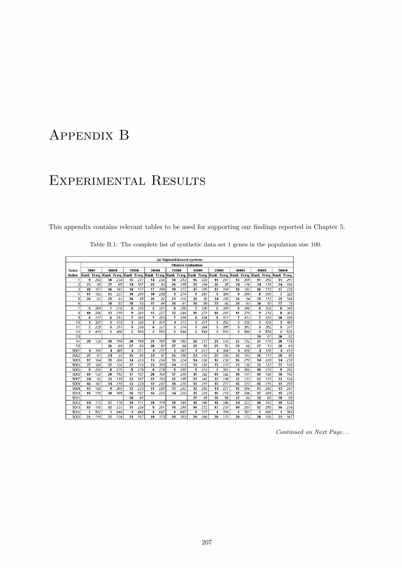
Appendix B
Experimental Results
This appendix contains relevant tables to be used for supporting our findings reported in Chapter 5.
Table B.1: The complete list of synthetic data set 1 genes in the population size 100.
Continued on Next Page. . .
207
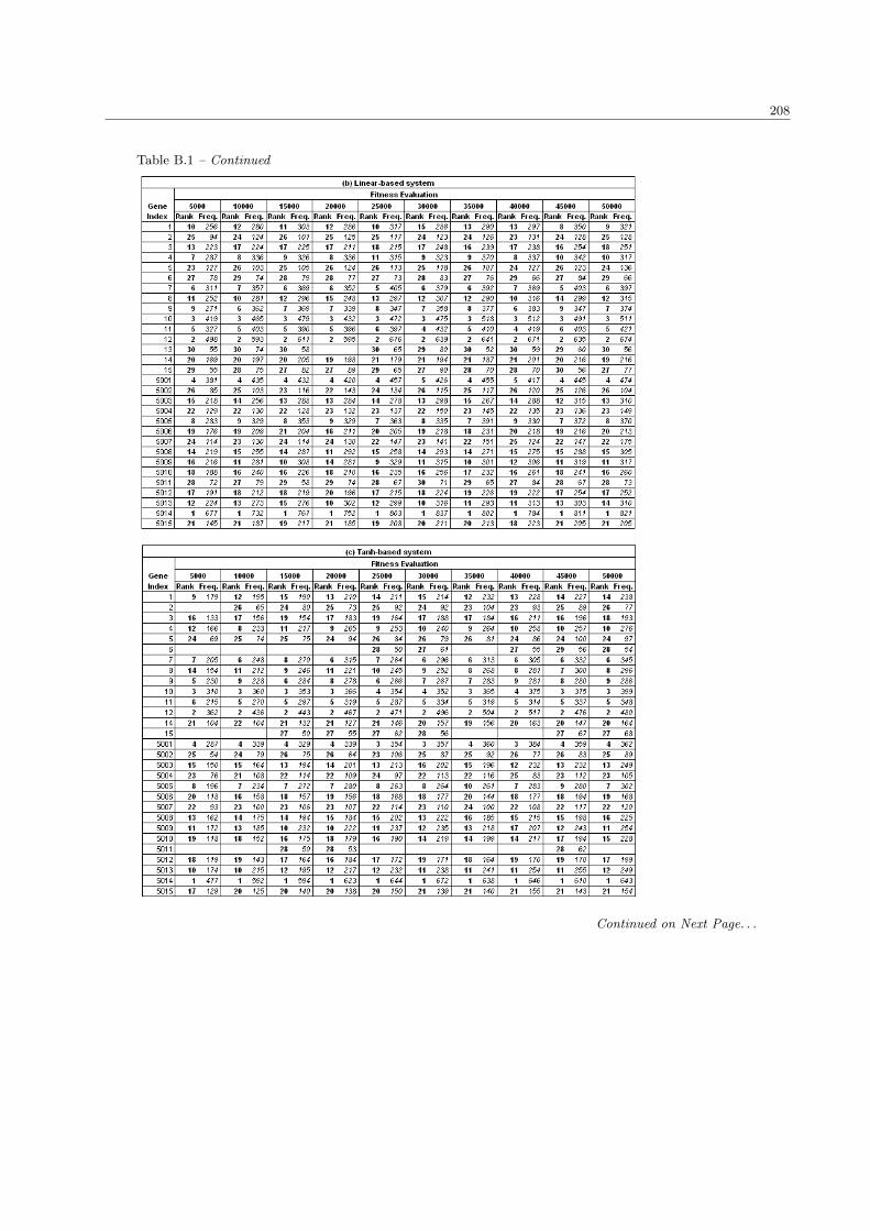
208
Table B.1 – Continued
Continued on Next Page. . .

209
Table B.1 – Continued
Table B.2: The complete list of synthetic data set 1 genes in the population size 200.
Continued on Next Page. . .
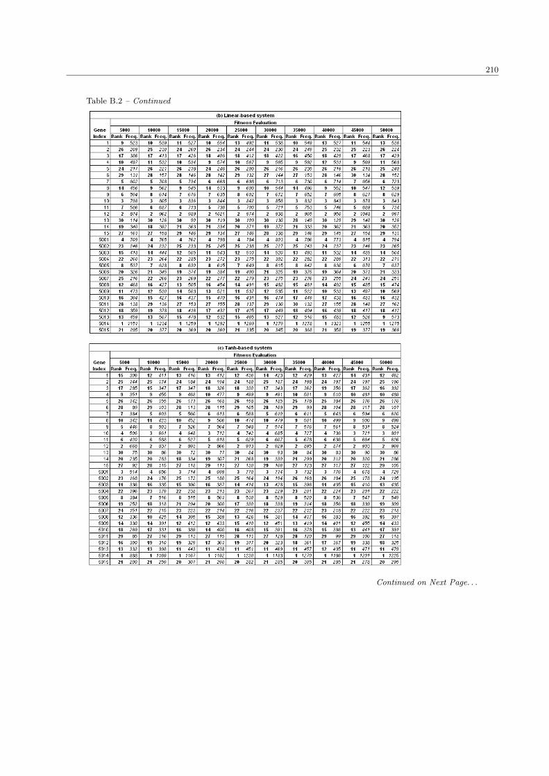
210
Table B.2 – Continued
Continued on Next Page. . .

211
Table B.2 – Continued
Table B.3: The complete list of synthetic data set 1 genes in the population size 300.
Continued on Next Page. . .
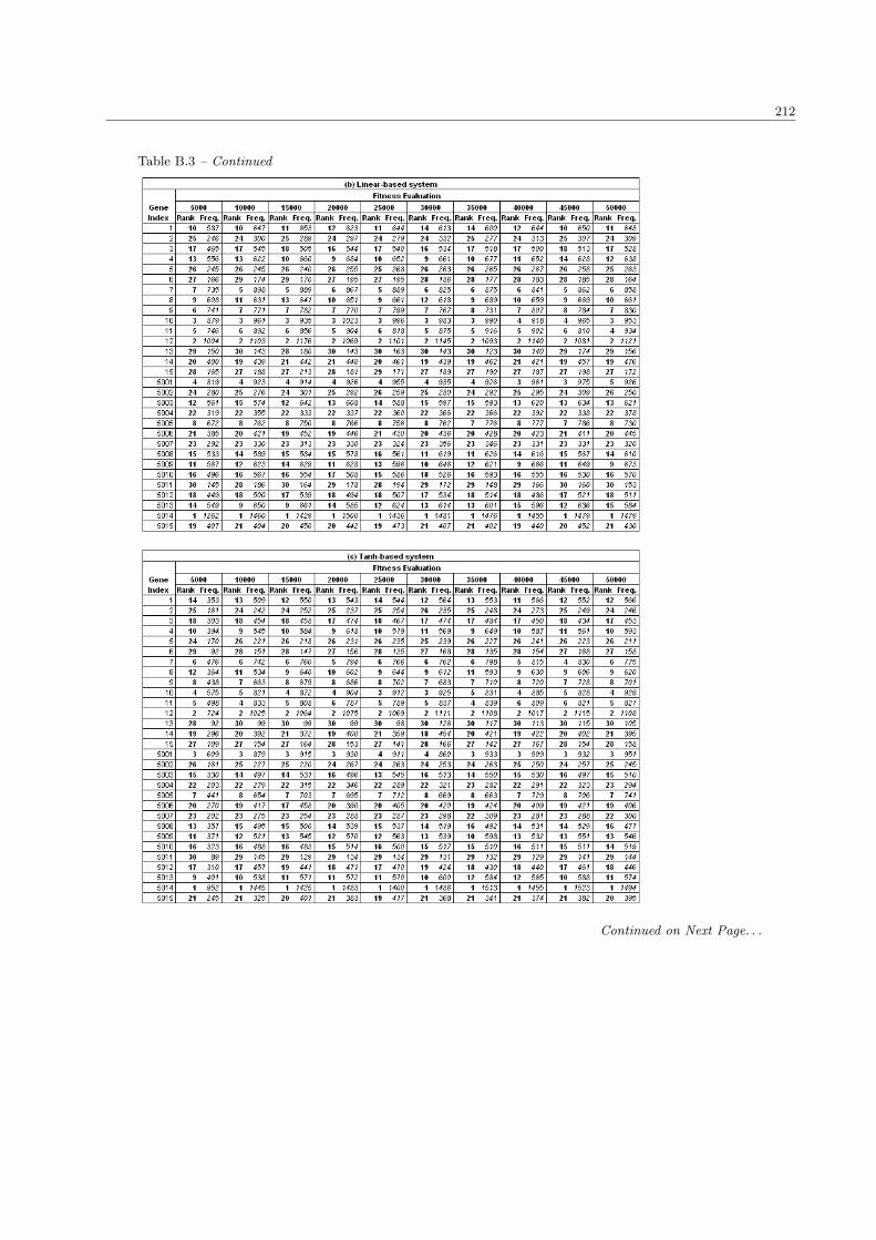
212
Table B.3 – Continued
Continued on Next Page. . .

213
Table B.3 – Continued

214
Table B.4: The complete list of synthetic data set 2 genes in the population size 100.
Table B.5: The complete list of synthetic data set 2 genes in the population size 200. Genes marked in reddenote noisy genes.
Continued on Next Page. . .

215
Table B.5 – Continued
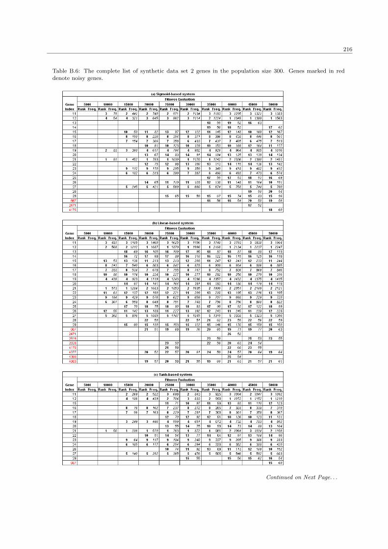
216
Table B.6: The complete list of synthetic data set 2 genes in the population size 300. Genes marked in reddenote noisy genes.
Continued on Next Page. . .
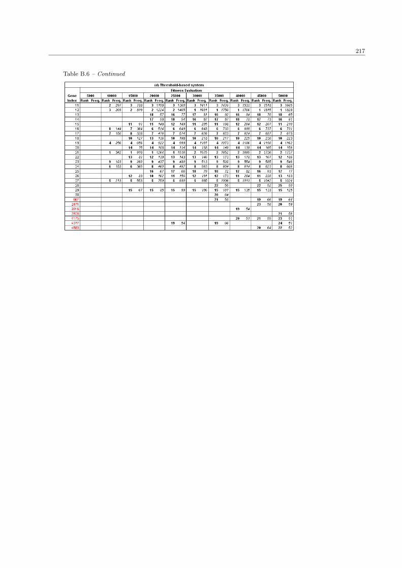
217
Table B.6 – Continued
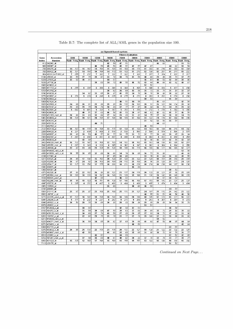
218
Table B.7: The complete list of ALL/AML genes in the population size 100.
Continued on Next Page. . .

219
Table B.7 – Continued
Continued on Next Page. . .
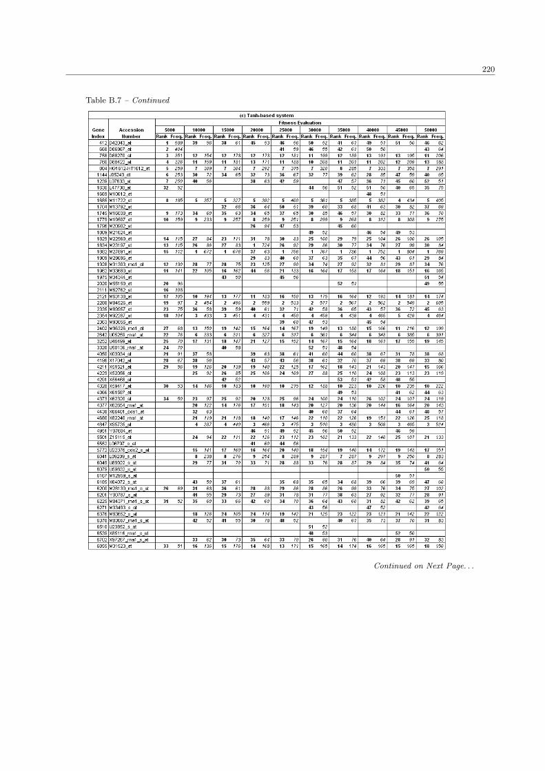
220
Table B.7 – Continued
Continued on Next Page. . .
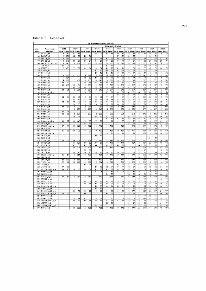
221
Table B.7 – Continued

222
Table B.8: The complete list of ALL/AML genes in the population size 200.
Continued on Next Page. . .

223
Table B.8 – Continued
Continued on Next Page. . .

224
Table B.8 – Continued
Continued on Next Page. . .

225
Table B.8 – Continued

226
Table B.9: The complete list of ALL/AML genes in the population size 300.
Continued on Next Page. . .
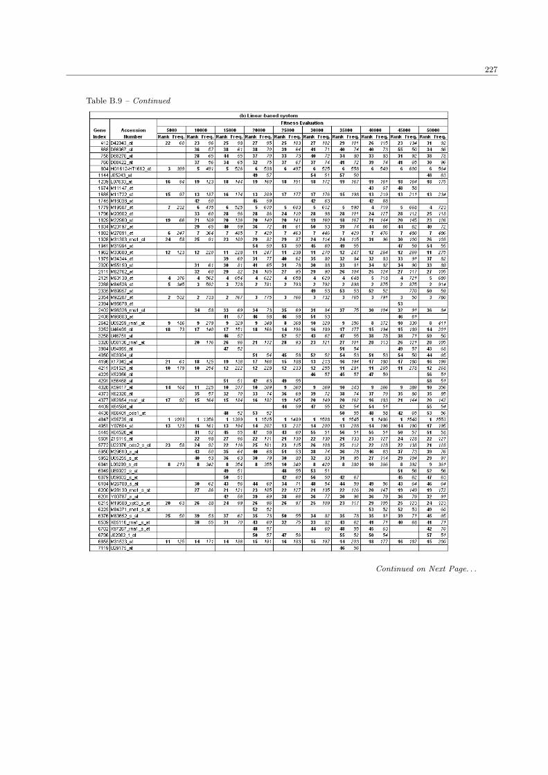
227
Table B.9 – Continued
Continued on Next Page. . .

228
Table B.9 – Continued
Continued on Next Page. . .

229
Table B.9 – Continued

230
Table B.10: The complete list of SRBCTs genes in the population size 100.
Continued on Next Page. . .
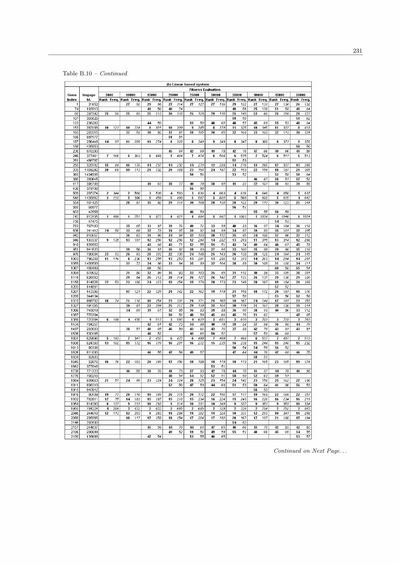
231
Table B.10 – Continued
Continued on Next Page. . .

232
Table B.10 – Continued
Continued on Next Page. . .

233
Table B.10 – Continued

234
Table B.11: The complete list of SRBCTs genes in the population size 200.
Continued on Next Page. . .

235
Table B.11 – Continued
Continued on Next Page. . .
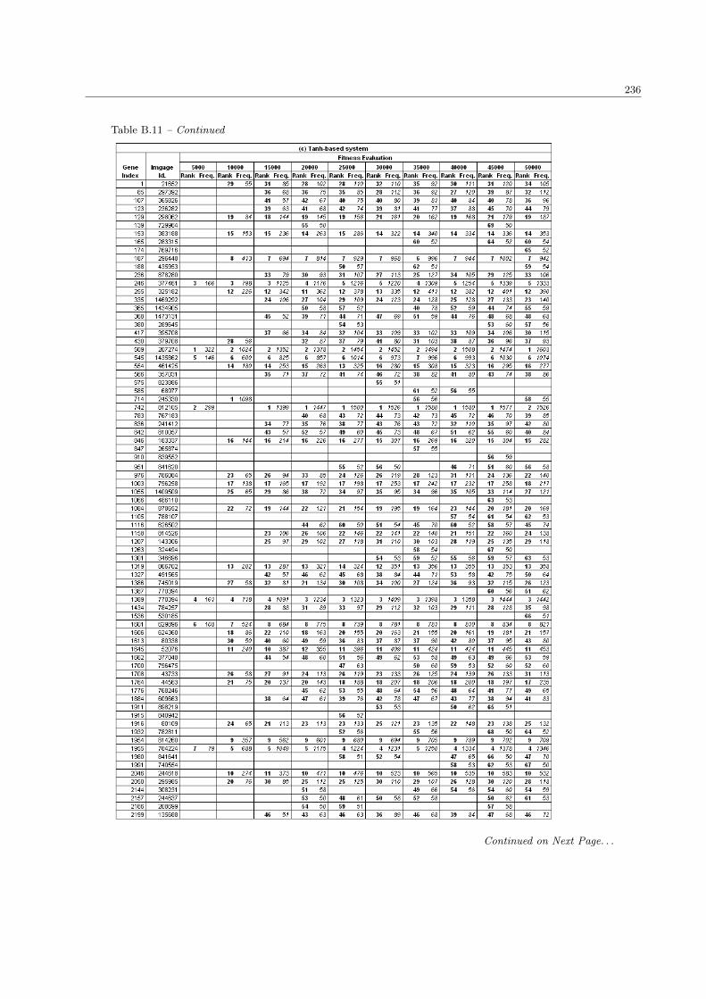
236
Table B.11 – Continued
Continued on Next Page. . .

237
Table B.11 – Continued
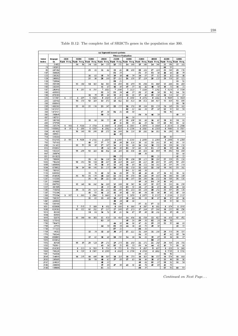
238
Table B.12: The complete list of SRBCTs genes in the population size 300.
Continued on Next Page. . .

239
Table B.12 – Continued
Continued on Next Page. . .

240
Table B.12 – Continued
Continued on Next Page. . .

241
Table B.12 – Continued
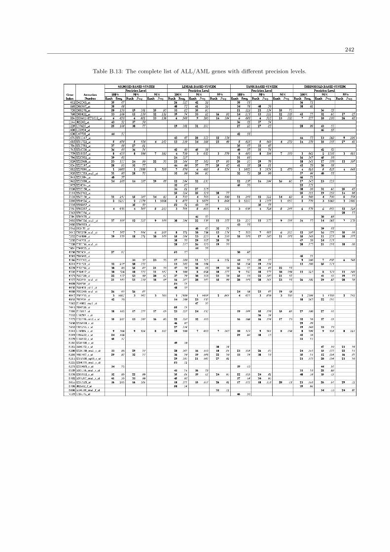
242
Table B.13: The complete list of ALL/AML genes with different precision levels.
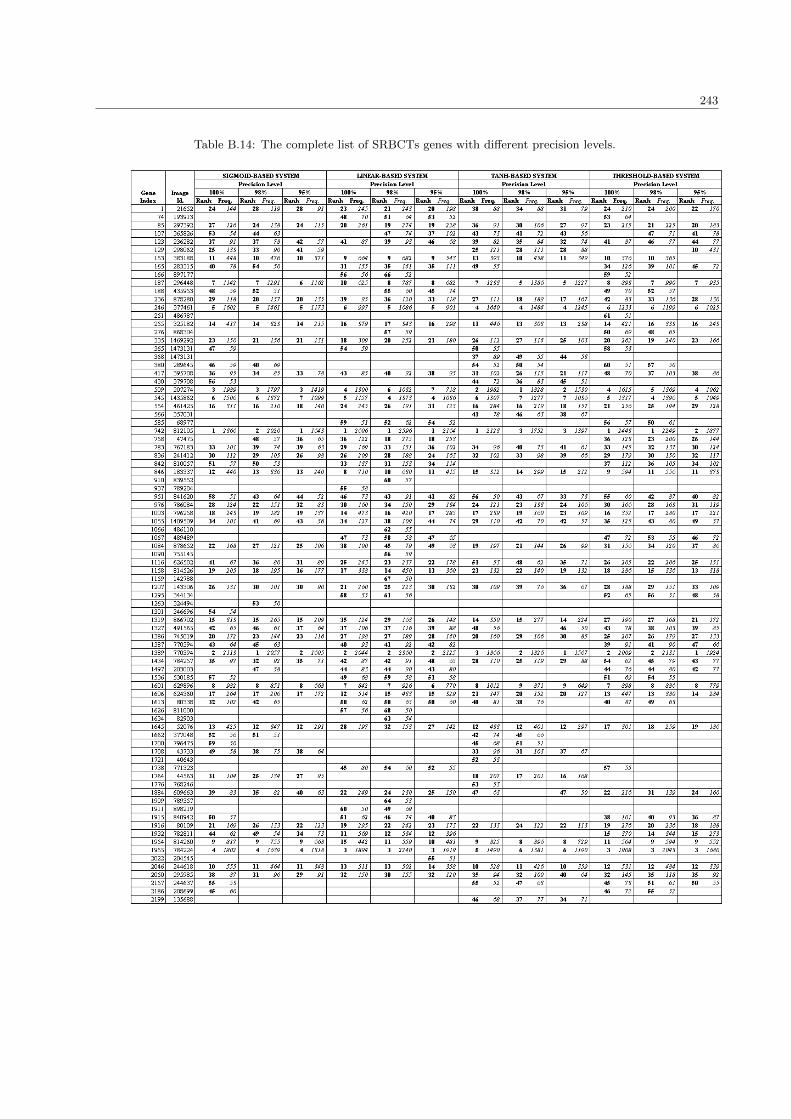
243
Table B.14: The complete list of SRBCTs genes with different precision levels.

244
Table B.15: The complete list of genes based on the raw and the normalised ALL/AML data sets.
Continued on Next Page. . .

245
Table B.15 – Continued

246T
able
B.1
6:
The
com
ple
telist
of
att
ribute
sse
lect
edby
GA
NN
inth
ebio
ass
aydata
set.
For
AID
362
data
set,
ato
p-2
8att
ribute
sw
ere
sele
cted
and
for
AID
688,
ato
p-3
1att
ribute
sw
ere
sele
cted
.
AID
362
AID
688
——
Ind
exA
ttri
bu
ted
escr
ipti
on
Data
typ
e—
—In
dex
Att
rib
ute
des
crip
tion
Data
typ
e—
—66
HB
D03
AR
CB
inary
——
147
PS
AR
eal
142
MW
Rea
l—
—151
MW
Rea
l57
HB
D05
HB
DB
inary
——
113
AR
C06
HY
PB
inary
139
Nu
mR
ot
Inte
ger
——
114
AR
C07
HY
PB
inary
93
AR
C01
AR
CB
inary
——
101
HB
A07
HY
PB
inary
143
BB
BB
inary
——
146
XL
ogP
Rea
l67
HB
D04
AR
CB
inary
——
112
AR
C05
HY
PB
inary
23
NE
G07
AR
CB
inary
——
107
AR
C06
AR
CB
inary
22
NE
G06
AR
CB
inary
——
89
HB
A06
HB
AB
inary
61
HB
D04
HB
AB
inary
——
98
HB
A04
HY
PB
inary
62
HB
D05
HB
AB
inary
——
119
HY
P05
HY
PB
inary
15
NE
G05
HB
AB
inary
——
131
WB
NE
NH
0.2
5R
eal
65
HB
D02
AR
CB
inary
——
106
AR
C05
AR
CB
inary
24
NE
G02
HY
PB
inary
——
99
HB
A05
HY
PB
inary
7N
EG
03
PO
SB
inary
——
86
HB
A03
HB
AB
inary
14
NE
G04
HB
AB
inary
——
95
HB
A07
AR
CB
inary
74
HB
D05
HY
PB
inary
——
42
PO
S03
HB
DB
inary
29
NE
G07
HY
PB
inary
——
74
HB
D02
AR
CB
inary
33
PO
S07
PO
SB
inary
——
103
AR
C02
AR
CB
inary
91
HB
A06
HY
PB
inary
——
148
Nu
mR
ot
Inte
ger
18
NE
G02
AR
CB
inary
——
153
Bad
Gro
up
Inte
ger
31
PO
S04
PO
SB
inary
——
32
NE
G03
HY
PB
inary
16
NE
G06
HB
AB
inary
——
64
HB
D03
HB
DB
inary
122
WB
NE
NH
0.2
5R
eal
——
79
HB
D07
AR
CB
inary
13
NE
G07
HB
DB
inary
——
25
NE
G02
AR
CB
inary
70
HB
D07
AR
CB
inary
——
91
HB
A03
AR
CB
inary
10
NE
G06
PO
SB
inary
——
39
PO
S05
PO
SB
inary
34
PO
S03
HB
DB
inary
——
40
PO
S06
PO
SB
inary
——
23
NE
G06
HB
AB
inary
——
96
HB
A02
HY
PB
inary
——
19
NE
G07
HB
DB
inary

Appendix C
Related Works
This appendix contains relevant studies in the microarray data sets that were being used in this thesis.
247

248T
able
C.1
:Som
ere
leva
nt
work
sin
AL
L/A
ML
mic
roarr
aydata
.
Au
thor
Data
pre
pro
cess
ing
No.
of
gen
esto
be
an
aly
sed
Met
hod
Valid
ati
on
mec
han
ism
Info
rmati
ve
gen
es
Cu
lhan
eet
al.
(2002)
No
tsp
ecifi
ed7159
CO
A/B
GA
;P
CA
/B
GA
LO
OC
V50
Bø
an
dJon
ass
en(2
002)
Sim
ilar
toD
ud
oit
etal.
(2002)
3934
vari
ety
sele
ctio
ns;
FD
A;
KN
N;
DL
DQ
Sam
ple
-sp
litt
ing;
LO
OC
V50
Li
etal.
(2001a)
Log
tran
sform
ati
on
7129
GA
/K
NN
Sam
ple
-sp
litt
ing
50
Du
doit
etal.
(2002)
Filte
rin
g;
log
tran
sform
ati
on
;n
orm
ali-
sati
on
3571
BS
S/W
SS
;D
T;
FD
A;
KN
NS
am
ple
-sp
litt
ing;
LO
OC
V40
Gu
yon
etal.
(2002)
Log
tran
sform
ati
on
;n
orm
alisa
tion
7129
SV
M/R
FE
Sam
ple
-sp
litt
ing;
LO
OC
V16
Li
an
dY
an
g(2
002)
Filte
rin
g;
log
tran
sform
ati
on
1000
LR
MS
am
ple
-sp
litt
ing
37
Tib
shir
an
iet
al.
(2002)
-7129
NS
CS
am
ple
-sp
litt
ing;
10-f
old
CV
21
Ch
oet
al.
(2003b
)N
ot
spec
ified
7129
FD
A5-f
old
CV
;L
OO
CV
6F
uts
chik
etal.
(2003)
Norm
alisa
tion
;lo
gtr
an
sform
ati
on
No
tsp
ecifi
edE
Fu
NN
;P
CA
;b
oots
trap
LO
OC
V;
N-f
old
CV
-L
eean
dL
ee(2
003)
Sim
ilar
toD
ud
oit
etal.
(2002)
3571
BS
S/W
SS
;S
VM
Sam
ple
-sp
litt
ing;
LO
OC
V40
Wan
get
al.
(2003)
Log
tran
sform
ati
on
;n
orm
alisa
tion
7129
SO
M;
fuzz
yC
-mea
ns
--
Li
etal.
(2004)
Norm
ali
sati
on
7129
vari
ety
sele
ctio
ns;
DT
;N
B;
SV
M;
KN
NS
am
ple
-sp
litt
ing;
4-f
old
CV
150
Web
eret
al.
(2004)
Filte
rin
g37
LR
M-
2C
hu
etal.
(2005)
Filte
rin
g;
norm
alisa
tion
1169
NB
;W
ilco
xon
ranksu
m10-f
old
CV
14
Dab
ney
(2005)
No
tsp
ecifi
ed3857
mod
ified
NS
C(C
laN
C)
No
tsp
ecifi
ed10
Jir
ap
ech
-Um
pai
an
dA
itken
(2005)
No
tsp
ecifi
ed7070
mod
ified
GE
SS
ES
;G
A/K
NN
Sam
ple
-sp
litt
ing;
LO
OC
V55
Mao
etal.
(2005)
Sim
ilar
toD
ud
oit
etal.
(2002)
3571
SV
M-R
FE
LO
OC
V20
Mra
mor
etal.
(2005)
No
tsp
ecifi
ed7074
Rel
iefF
;S
2N
-20
Takah
ash
iet
al.
(2005)
Filte
rin
g5401
Pro
ject
ive
ad
apti
ve
reso
nan
ceth
eory
(PA
RT
);fu
zzy
AN
NS
am
ple
-sp
litt
ing
10
Zh
ou
an
dM
ao
(2005)
Sim
ilar
toD
ud
oit
etal.
(2002);
filt
er-
ing
1000
Lea
stsq
uare
sS
VM
LO
OC
V12
Zh
ou
etal.
(2005)
Sim
ilar
toD
ud
oit
etal.
(2002)
3571
Bayes
ian
met
hod
sN
ot
Ap
pli
cabl
e20
Sakh
inia
etal.
(2006)
No
ta
pp
lica
ble
15
PC
R;
hou
sekee
pin
g;
Wilco
xon
ran
ksu
mN
ot
ap
pli
cabl
e15
Ch
oan
dW
on
(2007)
Norm
alisa
tion
7129
En
sem
ble
AN
Ns
Sam
ple
-sp
litt
ing
50
Xu
etal.
(2007)
Filte
rin
g1000
Part
icle
Sw
arm
Op
tim
isati
on
(PS
O);
Ellip
soid
AR
TM
AP
(EA
M)
10-f
old
CV
;L
OO
CV
63-9
7

249T
able
C.2
:Som
ere
leva
nt
work
sin
SR
BC
Ts
mic
roarr
aydata
.
Au
thor
Data
pre
pro
cess
ing
No.
of
gen
esto
be
an
aly
sed
Met
hod
Valid
ati
on
mec
han
ism
info
rmati
ve
gen
es
Lid
enet
al.
(2002)
-2308
Ru
le-i
nd
uct
ion
met
hod
s;IG
Sam
ple
-sp
litt
ing
32-1
28
Cu
lhan
eet
al.
(2002)
No
tsp
ecifi
ed2308
CO
A/B
GA
Sam
ple
-sp
litt
ing
50
Tib
shir
an
iet
al.
(2002)
-2308
NS
CS
am
ple
-sp
litt
ing;
10-f
old
CV
43
Ch
oet
al.
(2003b
)N
ot
spec
ified
2308
FD
A5-f
old
CV
;L
OO
CV
21
Deu
tsch
(2003)
-2308
GE
SS
ES
(EA
ap
pro
ach
)S
am
ple
-sp
litt
ing
15-2
8L
eean
dL
ee(2
003)
Log
tran
sform
ati
on
;n
orm
alisa
tion
2308
BS
S/W
SS
;S
VM
Sam
ple
-sp
litt
ing;
LO
OC
V20
Li
etal.
(2004)
Norm
ali
sati
on
2308
vari
ety
sele
ctio
ns;
DT
;N
B;
SV
M;
KN
NS
am
ple
-sp
litt
ing;
4-f
old
CV
150
Web
eret
al.
(2004)
Filte
rin
g62
LR
M-
7A
nd
rou
lakis
(2005)
No
tsp
ecifi
ed2303
En
sem
ble
Tre
esS
am
ple
-sp
litt
ing
3-1
9D
ab
ney
(2005)
No
tsp
ecifi
ed2307
mod
ified
NS
C(C
laN
C)
No
tsp
ecifi
ed8
Liu
etal.
(2005b
)L
og
tran
sform
ati
on
;n
orm
alisa
tion
2308
Entr
opy-b
ase
dco
rrel
ati
on
Sam
ple
-sp
litt
ing;
LO
OC
V58
Mao
etal.
(2005)
Filte
rin
g200
SV
M-R
FE
LO
OC
V20
Mra
mor
etal.
(2005)
No
tsp
ecifi
ed2308
Rel
iefF
;S
2N
-20
Ch
enet
al.
(2007)
No
ta
pp
lica
ble
39
PC
R;
hou
sekee
pin
ggen
es;
AN
NL
OO
CV
39
Pal
etal.
(2007)
-2308
fuzz
yC
-mea
ns/
AN
N;
RB
F;
SV
MS
am
ple
-sp
litt
ing
7-2
0
Wan
get
al.
(2007)
-2308
t-te
st;
fuzz
yA
NN
Sam
ple
-sp
litt
ing;
5-f
old
CV
50
Yu
etal.
(2007)
-2308
GP
;D
LD
A;
KN
NS
am
ple
-sp
litt
ing;
k-f
old
CV
54