bioinformatics ii: theoretical bioinformatics and machine learning · 2009-02-26 · bioinformatics...
TRANSCRIPT
Bioinformatics IITheoretical Bioinformatics and Machine Learning
Summer Semester 2009
by Sepp Hochreiter
Institute of Bioinformatics, Johannes Kepler University Linz
Lecture Notes
Institute of BioinformaticsJohannes Kepler University LinzA-4040 Linz, Austria
Tel. +43 732 2468 8880Fax +43 732 2468 9308
http://www.bioinf.jku.at

c© 2009 Sepp Hochreiter
This material, no matter whether in printed or electronic form, may be used for personal andeducational use only. Any reproduction of this manuscript, no matter whether as a whole or inparts, no matter whether in printed or in electronic form, requires explicit prior acceptance of theauthor.

Literature
Duda, Hart, Stork; Pattern Classification; Wiley & Sons, 2001
C. M. Bishop; Neural Networks for Pattern Recognition, Oxford University Press, 1995
Schölkopf, Smola; Learning with kernels, MIT Press, 2002
V. N. Vapnik; Statistical Learning Theory, Wiley & Sons, 1998
S. M. Kay; Fundamentals of Statistical Signal Processing, Prentice Hall, 1993
M. I. Jordan (ed.); Learning in Graphical Models, MIT Press, 1998 (Original by KluwerAcademic Pub.)
T. M. Mitchell; Machine Learning, Mc Graw Hill, 1997
R. M. Neal, Bayesian Learning for Neural Networks, Springer, (Lecture Notes in Statistics),1996
Guyon, Gunn, Nikravesh, Zadeh (eds.); Feature Extraction - Foundations and Applications,Springer, 2006
Schölkopf, Tsuda, Vert (eds.); Kernel Methods in Computational Biology, MIT Press, 2003
iii

iv

Contents
1 Introduction 1
2 Basics of Machine Learning 32.1 Machine Learning in Bioinformatics . . . . . . . . . . . . . . . . . . . . . . . . 32.2 Introductory Example . . . . . . . . . . . . . . . . . . . . . . . . . . . . . . . . 42.3 Supervised and Unsupervised Learning . . . . . . . . . . . . . . . . . . . . . . 92.4 Reinforcement Learning . . . . . . . . . . . . . . . . . . . . . . . . . . . . . . 132.5 Feature Extraction, Selection, and Construction . . . . . . . . . . . . . . . . . . 142.6 Parametric vs. Non-Parametric Models . . . . . . . . . . . . . . . . . . . . . . . 192.7 Generative vs. descriptive Models . . . . . . . . . . . . . . . . . . . . . . . . . 202.8 Prior and Domain Knowledge . . . . . . . . . . . . . . . . . . . . . . . . . . . 212.9 Model Selection and Training . . . . . . . . . . . . . . . . . . . . . . . . . . . . 212.10 Model Evaluation, Hyperparameter Selection, and Final Model . . . . . . . . . . 23
3 Theoretical Background of Machine Learning 273.1 Model Quality Criteria . . . . . . . . . . . . . . . . . . . . . . . . . . . . . . . 283.2 Generalization error . . . . . . . . . . . . . . . . . . . . . . . . . . . . . . . . . 29
3.2.1 Definition of the Generalization Error / Risk . . . . . . . . . . . . . . . . 293.2.2 Empirical Estimation of the Generalization Error . . . . . . . . . . . . . 31
3.2.2.1 Test Set . . . . . . . . . . . . . . . . . . . . . . . . . . . . . 313.2.2.2 Cross-Validation . . . . . . . . . . . . . . . . . . . . . . . . . 31
3.3 Minimal Risk for a Gaussian Classification Task . . . . . . . . . . . . . . . . . . 343.4 Maximum Likelihood . . . . . . . . . . . . . . . . . . . . . . . . . . . . . . . . 41
3.4.1 Loss for Unsupervised Learning . . . . . . . . . . . . . . . . . . . . . . 413.4.1.1 Projection Methods . . . . . . . . . . . . . . . . . . . . . . . 413.4.1.2 Generative Model . . . . . . . . . . . . . . . . . . . . . . . . 413.4.1.3 Parameter Estimation . . . . . . . . . . . . . . . . . . . . . . 43
3.4.2 Mean Squared Error, Bias, and Variance . . . . . . . . . . . . . . . . . . 443.4.3 Fisher Information Matrix, Cramer-Rao Lower Bound, and Efficiency . . 463.4.4 Maximum Likelihood Estimator . . . . . . . . . . . . . . . . . . . . . . 483.4.5 Properties of Maximum Likelihood Estimator . . . . . . . . . . . . . . . 49
3.4.5.1 MLE is Invariant under Parameter Change . . . . . . . . . . . 493.4.5.2 MLE is Asymptotically Unbiased and Efficient . . . . . . . . . 493.4.5.3 MLE is Consistent for Zero CRLB . . . . . . . . . . . . . . . 50
3.4.6 Expectation Maximization . . . . . . . . . . . . . . . . . . . . . . . . . 513.5 Noise Models . . . . . . . . . . . . . . . . . . . . . . . . . . . . . . . . . . . . 54
v

3.5.1 Gaussian Noise . . . . . . . . . . . . . . . . . . . . . . . . . . . . . . . 543.5.2 Laplace Noise and Minkowski Error . . . . . . . . . . . . . . . . . . . . 563.5.3 Binary Models . . . . . . . . . . . . . . . . . . . . . . . . . . . . . . . 57
3.5.3.1 Cross-Entropy . . . . . . . . . . . . . . . . . . . . . . . . . . 573.5.3.2 Logistic Regression . . . . . . . . . . . . . . . . . . . . . . . 583.5.3.3 (Regularized) Linear Logistic Regression is Strictly Convex . . 623.5.3.4 Softmax . . . . . . . . . . . . . . . . . . . . . . . . . . . . . 633.5.3.5 (Regularized) Linear Softmax is Strictly Convex . . . . . . . . 64
3.6 Statistical Learning Theory . . . . . . . . . . . . . . . . . . . . . . . . . . . . . 663.6.1 Error Bounds for a Gaussian Classification Task . . . . . . . . . . . . . 663.6.2 Empirical Risk Minimization . . . . . . . . . . . . . . . . . . . . . . . . 67
3.6.2.1 Complexity: Finite Number of Functions . . . . . . . . . . . . 683.6.2.2 Complexity: VC-Dimension . . . . . . . . . . . . . . . . . . 70
3.6.3 Error Bounds . . . . . . . . . . . . . . . . . . . . . . . . . . . . . . . . 753.6.4 Structural Risk Minimization . . . . . . . . . . . . . . . . . . . . . . . . 783.6.5 Margin as Complexity Measure . . . . . . . . . . . . . . . . . . . . . . 80
4 Support Vector Machines 874.1 Support Vector Machines in Bioinformatics . . . . . . . . . . . . . . . . . . . . 874.2 Linearly Separable Problems . . . . . . . . . . . . . . . . . . . . . . . . . . . . 894.3 Linear SVM . . . . . . . . . . . . . . . . . . . . . . . . . . . . . . . . . . . . . 914.4 Linear SVM for Non-Linear Separable Problems . . . . . . . . . . . . . . . . . 954.5 Average Error Bounds for SVMs . . . . . . . . . . . . . . . . . . . . . . . . . . 1014.6 ν-SVM . . . . . . . . . . . . . . . . . . . . . . . . . . . . . . . . . . . . . . . 1034.7 Non-Linear SVM and the Kernel Trick . . . . . . . . . . . . . . . . . . . . . . . 1064.8 Other Interpretation of the Kernel: Reproducing Kernel Hilbert Space . . . . . . 1184.9 Example: Face Recognition . . . . . . . . . . . . . . . . . . . . . . . . . . . . . 1204.10 Multi-Class SVM . . . . . . . . . . . . . . . . . . . . . . . . . . . . . . . . . . 1214.11 Support Vector Regression . . . . . . . . . . . . . . . . . . . . . . . . . . . . . 1284.12 One Class SVM . . . . . . . . . . . . . . . . . . . . . . . . . . . . . . . . . . . 1384.13 Least Squares SVM . . . . . . . . . . . . . . . . . . . . . . . . . . . . . . . . . 1434.14 Potential Support Vector Machine . . . . . . . . . . . . . . . . . . . . . . . . . 1454.15 SVM Optimization and SMO . . . . . . . . . . . . . . . . . . . . . . . . . . . . 151
4.15.1 Convex Optimization . . . . . . . . . . . . . . . . . . . . . . . . . . . . 1514.15.2 Sequential Minimal Optimization . . . . . . . . . . . . . . . . . . . . . 160
4.16 Designing Kernels for Bioinformatics Applications . . . . . . . . . . . . . . . . 1644.16.1 String Kernel . . . . . . . . . . . . . . . . . . . . . . . . . . . . . . . . 1644.16.2 Spectrum Kernel . . . . . . . . . . . . . . . . . . . . . . . . . . . . . . 1654.16.3 Mismatch Kernel . . . . . . . . . . . . . . . . . . . . . . . . . . . . . . 1654.16.4 Motif Kernel . . . . . . . . . . . . . . . . . . . . . . . . . . . . . . . . 1654.16.5 Pairwise Kernel . . . . . . . . . . . . . . . . . . . . . . . . . . . . . . . 1654.16.6 Local Alignment Kernel . . . . . . . . . . . . . . . . . . . . . . . . . . 1664.16.7 Smith-Waterman Kernel . . . . . . . . . . . . . . . . . . . . . . . . . . 1664.16.8 Fisher Kernel . . . . . . . . . . . . . . . . . . . . . . . . . . . . . . . . 1664.16.9 Profile and PSSM Kernels . . . . . . . . . . . . . . . . . . . . . . . . . 1674.16.10 Kernels Based on Chemical Properties . . . . . . . . . . . . . . . . . . . 167
vi

4.16.11 Local DNA Kernel . . . . . . . . . . . . . . . . . . . . . . . . . . . . . 1674.16.12 Salzberg DNA Kernel . . . . . . . . . . . . . . . . . . . . . . . . . . . 1674.16.13 Shifted Weighted Degree Kernel . . . . . . . . . . . . . . . . . . . . . . 167
4.17 Kernel Principal Component Analysis . . . . . . . . . . . . . . . . . . . . . . . 1674.18 Kernel Discriminant Analysis . . . . . . . . . . . . . . . . . . . . . . . . . . . . 1714.19 Software . . . . . . . . . . . . . . . . . . . . . . . . . . . . . . . . . . . . . . . 178
5 Error Minimization and Model Selection 1795.1 Search Methods and Evolutionary Approaches . . . . . . . . . . . . . . . . . . . 1795.2 Gradient Descent . . . . . . . . . . . . . . . . . . . . . . . . . . . . . . . . . . 1815.3 Step-size Optimization . . . . . . . . . . . . . . . . . . . . . . . . . . . . . . . 182
5.3.1 Heuristics . . . . . . . . . . . . . . . . . . . . . . . . . . . . . . . . . . 1845.3.2 Line Search . . . . . . . . . . . . . . . . . . . . . . . . . . . . . . . . . 186
5.4 Optimization of the Update Direction . . . . . . . . . . . . . . . . . . . . . . . 1885.4.1 Newton and Quasi-Newton Method . . . . . . . . . . . . . . . . . . . . 1885.4.2 Conjugate Gradient . . . . . . . . . . . . . . . . . . . . . . . . . . . . . 190
5.5 Levenberg-Marquardt Algorithm . . . . . . . . . . . . . . . . . . . . . . . . . . 1945.6 Predictor Corrector Methods for R(w) = 0 . . . . . . . . . . . . . . . . . . . . 1955.7 Convergence Properties . . . . . . . . . . . . . . . . . . . . . . . . . . . . . . . 1955.8 On-line Optimization . . . . . . . . . . . . . . . . . . . . . . . . . . . . . . . . 198
6 Neural Networks 2016.1 Neural Networks in Bioinformatics . . . . . . . . . . . . . . . . . . . . . . . . . 2016.2 Principles of Neural Networks . . . . . . . . . . . . . . . . . . . . . . . . . . . 2036.3 Linear Neurons and the Perceptron . . . . . . . . . . . . . . . . . . . . . . . . . 2056.4 Multi-Layer Perceptron . . . . . . . . . . . . . . . . . . . . . . . . . . . . . . . 208
6.4.1 Architecture and Activation Functions . . . . . . . . . . . . . . . . . . . 2086.4.2 Universality . . . . . . . . . . . . . . . . . . . . . . . . . . . . . . . . . 2116.4.3 Learning and Back-Propagation . . . . . . . . . . . . . . . . . . . . . . 2126.4.4 Hessian . . . . . . . . . . . . . . . . . . . . . . . . . . . . . . . . . . . 2156.4.5 Regularization . . . . . . . . . . . . . . . . . . . . . . . . . . . . . . . 224
6.4.5.1 Early Stopping . . . . . . . . . . . . . . . . . . . . . . . . . . 2256.4.5.2 Growing: Cascade-Correlation . . . . . . . . . . . . . . . . . 2266.4.5.3 Pruning: OBS and OBD . . . . . . . . . . . . . . . . . . . . . 2266.4.5.4 Weight Decay . . . . . . . . . . . . . . . . . . . . . . . . . . 2306.4.5.5 Training with Noise . . . . . . . . . . . . . . . . . . . . . . . 2316.4.5.6 Weight Sharing . . . . . . . . . . . . . . . . . . . . . . . . . 2316.4.5.7 Flat Minimum Search . . . . . . . . . . . . . . . . . . . . . . 2326.4.5.8 Regularization for Structure Extraction . . . . . . . . . . . . . 233
6.4.6 Tricks of the Trade . . . . . . . . . . . . . . . . . . . . . . . . . . . . . 2356.4.6.1 Number of Training Examples . . . . . . . . . . . . . . . . . 2356.4.6.2 Committees . . . . . . . . . . . . . . . . . . . . . . . . . . . 2406.4.6.3 Local Minima . . . . . . . . . . . . . . . . . . . . . . . . . . 2416.4.6.4 Initialization . . . . . . . . . . . . . . . . . . . . . . . . . . . 2416.4.6.5 δ-Propagation . . . . . . . . . . . . . . . . . . . . . . . . . . 2426.4.6.6 Input Scaling . . . . . . . . . . . . . . . . . . . . . . . . . . . 2426.4.6.7 Targets . . . . . . . . . . . . . . . . . . . . . . . . . . . . . . 242
vii

6.4.6.8 Learning Rate . . . . . . . . . . . . . . . . . . . . . . . . . . 2426.4.6.9 Number of Hidden Units and Layers . . . . . . . . . . . . . . 2436.4.6.10 Momentum and Weight Decay . . . . . . . . . . . . . . . . . 2436.4.6.11 Stopping . . . . . . . . . . . . . . . . . . . . . . . . . . . . . 2436.4.6.12 Batch vs. On-line . . . . . . . . . . . . . . . . . . . . . . . . 243
6.5 Radial Basis Function Networks . . . . . . . . . . . . . . . . . . . . . . . . . . 2446.5.1 Clustering and Least Squares Estimate . . . . . . . . . . . . . . . . . . . 2456.5.2 Gradient Descent . . . . . . . . . . . . . . . . . . . . . . . . . . . . . . 2456.5.3 Curse of Dimensionality . . . . . . . . . . . . . . . . . . . . . . . . . . 246
6.6 Recurrent Neural Networks . . . . . . . . . . . . . . . . . . . . . . . . . . . . . 2466.6.1 Sequence Processing with RNNs . . . . . . . . . . . . . . . . . . . . . . 2476.6.2 Real-Time Recurrent Learning . . . . . . . . . . . . . . . . . . . . . . . 2486.6.3 Back-Propagation Through Time . . . . . . . . . . . . . . . . . . . . . . 2496.6.4 Other Approaches . . . . . . . . . . . . . . . . . . . . . . . . . . . . . 2536.6.5 Vanishing Gradient . . . . . . . . . . . . . . . . . . . . . . . . . . . . . 2546.6.6 Long Short-Term Memory . . . . . . . . . . . . . . . . . . . . . . . . . 255
7 Bayes Techniques 2617.1 Likelihood, Prior, Posterior, Evidence . . . . . . . . . . . . . . . . . . . . . . . 2627.2 Maximum A Posteriori Approach . . . . . . . . . . . . . . . . . . . . . . . . . 2647.3 Posterior Approximation . . . . . . . . . . . . . . . . . . . . . . . . . . . . . . 2667.4 Error Bars and Confidence Intervals . . . . . . . . . . . . . . . . . . . . . . . . 2677.5 Hyper-parameter Selection: Evidence Framework . . . . . . . . . . . . . . . . . 2697.6 Hyper-parameter Selection: Integrate Out . . . . . . . . . . . . . . . . . . . . . 2727.7 Model Comparison . . . . . . . . . . . . . . . . . . . . . . . . . . . . . . . . . 2737.8 Posterior Sampling . . . . . . . . . . . . . . . . . . . . . . . . . . . . . . . . . 274
8 Feature Selection 2778.1 Feature Selection in Bioinformatics . . . . . . . . . . . . . . . . . . . . . . . . 277
8.1.1 Mass Spectrometry . . . . . . . . . . . . . . . . . . . . . . . . . . . . . 2788.1.2 Protein Sequences . . . . . . . . . . . . . . . . . . . . . . . . . . . . . 2788.1.3 Microarray Data . . . . . . . . . . . . . . . . . . . . . . . . . . . . . . 279
8.2 Feature Selection Methods . . . . . . . . . . . . . . . . . . . . . . . . . . . . . 2828.2.1 Filter Methods . . . . . . . . . . . . . . . . . . . . . . . . . . . . . . . 2838.2.2 Wrapper Methods . . . . . . . . . . . . . . . . . . . . . . . . . . . . . . 2888.2.3 Kernel Based Methods . . . . . . . . . . . . . . . . . . . . . . . . . . . 289
8.2.3.1 Feature selection after learning . . . . . . . . . . . . . . . . . 2898.2.3.2 Feature selection during learning . . . . . . . . . . . . . . . . 2898.2.3.3 P-SVM Feature Selection . . . . . . . . . . . . . . . . . . . . 290
8.2.4 Automatic Relevance Determination . . . . . . . . . . . . . . . . . . . . 2918.3 Microarray Gene Selection Protocol . . . . . . . . . . . . . . . . . . . . . . . . 292
8.3.1 Description of the Protocol . . . . . . . . . . . . . . . . . . . . . . . . . 2928.3.2 Comments on the Protocol and on Gene Selection . . . . . . . . . . . . . 2948.3.3 Classification of Samples . . . . . . . . . . . . . . . . . . . . . . . . . . 295
viii

9 Hidden Markov Models 2979.1 Hidden Markov Models in Bioinformatics . . . . . . . . . . . . . . . . . . . . . 2979.2 Hidden Markov Model Basics . . . . . . . . . . . . . . . . . . . . . . . . . . . 2989.3 Expectation Maximization for HMM: Baum-Welch Algorithm . . . . . . . . . . 3049.4 Viterby Algorithm . . . . . . . . . . . . . . . . . . . . . . . . . . . . . . . . . . 3079.5 Input Output Hidden Markov Models . . . . . . . . . . . . . . . . . . . . . . . 3109.6 Factorial Hidden Markov Models . . . . . . . . . . . . . . . . . . . . . . . . . . 3129.7 Memory Input Output Factorial Hidden Markov Models . . . . . . . . . . . . . 3129.8 Tricks of the Trade . . . . . . . . . . . . . . . . . . . . . . . . . . . . . . . . . 3149.9 Profile Hidden Markov Models . . . . . . . . . . . . . . . . . . . . . . . . . . . 315
10 Unsupervised Learning: Projection Methods and Clustering 31910.1 Introduction . . . . . . . . . . . . . . . . . . . . . . . . . . . . . . . . . . . . . 319
10.1.1 Unsupervised Learning in Bioinformatics . . . . . . . . . . . . . . . . . 31910.1.2 Unsupervised Learning Categories . . . . . . . . . . . . . . . . . . . . . 319
10.1.2.1 Generative Framework . . . . . . . . . . . . . . . . . . . . . 32010.1.2.2 Recoding Framework . . . . . . . . . . . . . . . . . . . . . . 32010.1.2.3 Recoding and Generative Framework Unified . . . . . . . . . 324
10.2 Principal Component Analysis . . . . . . . . . . . . . . . . . . . . . . . . . . . 32510.3 Independent Component Analysis . . . . . . . . . . . . . . . . . . . . . . . . . 327
10.3.1 Measuring Independence . . . . . . . . . . . . . . . . . . . . . . . . . . 32910.3.2 INFOMAX Algorithm . . . . . . . . . . . . . . . . . . . . . . . . . . . 33110.3.3 EASI Algorithm . . . . . . . . . . . . . . . . . . . . . . . . . . . . . . 33310.3.4 FastICA Algorithm . . . . . . . . . . . . . . . . . . . . . . . . . . . . . 333
10.4 Factor Analysis . . . . . . . . . . . . . . . . . . . . . . . . . . . . . . . . . . . 33310.5 Projection Pursuit and Multidimensional Scaling . . . . . . . . . . . . . . . . . 340
10.5.1 Projection Pursuit . . . . . . . . . . . . . . . . . . . . . . . . . . . . . . 34010.5.2 Multidimensional Scaling . . . . . . . . . . . . . . . . . . . . . . . . . 340
10.6 Clustering . . . . . . . . . . . . . . . . . . . . . . . . . . . . . . . . . . . . . . 34110.6.1 Mixture Models . . . . . . . . . . . . . . . . . . . . . . . . . . . . . . . 34210.6.2 k-Means Clustering . . . . . . . . . . . . . . . . . . . . . . . . . . . . . 34610.6.3 Hierarchical Clustering . . . . . . . . . . . . . . . . . . . . . . . . . . . 34810.6.4 Self-Organizing Maps . . . . . . . . . . . . . . . . . . . . . . . . . . . 350
ix

x

List of Figures
2.1 Salmons must be distinguished from sea bass. . . . . . . . . . . . . . . . . . . . 52.2 Salmon and see bass are separated by their length. . . . . . . . . . . . . . . . . . 62.3 Salmon and see bass are separated by their lightness. . . . . . . . . . . . . . . . 72.4 Salmon and see bass are separated by their lightness and their width. . . . . . . . 72.5 Salmon and see bass are separated by a nonlinear curve in the two-dimensional
space spanned by the lightness and the width of the fishes. . . . . . . . . . . . . 82.6 Salmon and see bass are separated by a nonlinear curve in the two-dimensional
space spanned by the lightness and the width of the fishes. . . . . . . . . . . . . 92.7 Example of a clustering algorithm. . . . . . . . . . . . . . . . . . . . . . . . . . 112.8 Example of a clustering algorithm where the clusters have different shape. . . . . 112.9 Example of a clustering where the clusters have a non-elliptical shape and cluster-
ing methods fail to extract the clusters. . . . . . . . . . . . . . . . . . . . . . . 122.10 Two speakers recorded by two microphones. . . . . . . . . . . . . . . . . . . . . 122.11 On top the data points where the components are correlated. . . . . . . . . . . . 132.12 Images of fMRI brain data together with EEG data. . . . . . . . . . . . . . . . . 142.13 Another image of fMRI brain data together with EEG data. . . . . . . . . . . . . 152.14 Simple two feature classification problem, where feature 1 (var. 1) is noise and
feature 2 (var. 2) is correlated to the classes. . . . . . . . . . . . . . . . . . . . . 162.15 The design cycle for machine learning in order to solve a certain task. . . . . . . 172.16 An XOR problem of two features. . . . . . . . . . . . . . . . . . . . . . . . . . 182.17 The left and right subfigure shows each two classes where the features mean value
and variance for each class is equal. . . . . . . . . . . . . . . . . . . . . . . . . 182.18 The trade-off between underfitting and overfitting is shown. . . . . . . . . . . . . 22
3.1 Cross-validation: The data set is divided into 5 parts. . . . . . . . . . . . . . . . 323.2 Cross-validation: For 5-fold cross-validation there are 5 iterations. . . . . . . . . 323.3 Linear transformations of the Gaussian N (µ,Σ). . . . . . . . . . . . . . . . . . 353.4 A two-dimensional classification task where the data for each class are drawn from
a Gaussian. . . . . . . . . . . . . . . . . . . . . . . . . . . . . . . . . . . . . . 363.5 Posterior densities p(y = 1 | x) and p(y = −1 | x) as a function of x. . . . . . . 383.6 x∗ is a non-optimal decision point because for some regions the posterior y = 1 is
above the posterior y = −1 but data is classified as y = −1. . . . . . . . . . . . 383.7 Two classes with covariance matrix Σ = σ2I each in one (top left), two (top
right), and three (bottom) dimensions. . . . . . . . . . . . . . . . . . . . . . . . 403.8 Two classes with arbitrary Gaussian covariance lead to boundary functions which
are hyperplanes, hyper-ellipsoids, hyperparaboloids etc. . . . . . . . . . . . . . . 42
xi

3.9 Projection model, where the observed data x is the input to the model u = g(x;w). 433.10 Generative model, where the data x is observed and the model x = g(u;w)
should produce the same distribution as the observed distribution. . . . . . . . . 433.11 The variance of an estimator w as a curve of the true parameter is shown. . . . . 483.12 The maximum likelihood problem. . . . . . . . . . . . . . . . . . . . . . . . . . 513.13 Different noise assumptions lead to different Minkowski error functions. . . . . . 573.14 The sigmoidal function 1
1+exp(−x) . . . . . . . . . . . . . . . . . . . . . . . . . . 583.15 Typical example where the test error first decreases and then increases with in-
creasing complexity. . . . . . . . . . . . . . . . . . . . . . . . . . . . . . . . . 693.16 The consistency of the empirical risk minimization is depicted. . . . . . . . . . . 713.17 Linear decision boundaries can shatter any 3 points in a 2-dimensional space. . . 723.18 Linear decision boundaries cannot shatter any 4 points in a 2-dimensional space. 723.19 The growth function is either linear or logarithmic in l. . . . . . . . . . . . . . . 743.20 The error bound is the sum of the empirical error, the training error, and a com-
plexity term. . . . . . . . . . . . . . . . . . . . . . . . . . . . . . . . . . . . . . 773.21 The bound on the risk, the test error, is depicted. . . . . . . . . . . . . . . . . . . 783.22 The structural risk minimization principle is based on a structure on a set of func-
tions which is nested subsets Fn of functions. . . . . . . . . . . . . . . . . . . . 793.23 Data points are contained in a sphere of radius R at the origin. . . . . . . . . . . 803.24 Margin means that hyperplanes must keep outside the spheres. . . . . . . . . . . 813.25 The offset b is optimized in order to obtain the largest ‖w‖ for the canonical form
which is ‖w∗‖ for the optimal value b∗. . . . . . . . . . . . . . . . . . . . . . . 82
4.1 A linearly separable problem. . . . . . . . . . . . . . . . . . . . . . . . . . . . . 904.2 Different solutions for linearly separating the the classes. . . . . . . . . . . . . . 904.3 Intuitively, better generalization is expected from separation on the right hand side
than from the left hand side. . . . . . . . . . . . . . . . . . . . . . . . . . . . . 914.4 For the hyperplane described by the canonical discriminant function and for the
optimal offset b (same distance to class 1 and class 2), the margin is γ = 1‖w‖ . . 92
4.5 Two examples for linear SVMs. . . . . . . . . . . . . . . . . . . . . . . . . . . 964.6 Left: linear separable task. Right: a task which is not linearly separable. . . . . . 964.7 Two problems at the top line which are not linearly separable. . . . . . . . . . . 974.8 Typical situation for the C-SVM. . . . . . . . . . . . . . . . . . . . . . . . . . . 1014.9 Essential vectors. . . . . . . . . . . . . . . . . . . . . . . . . . . . . . . . . . . 1024.10 Nonlinearly separable data is mapped into a feature space where the data is linear
separable. . . . . . . . . . . . . . . . . . . . . . . . . . . . . . . . . . . . . . . 1074.11 An example of a mapping from the two-dimensional space into the three-dimensional
space. . . . . . . . . . . . . . . . . . . . . . . . . . . . . . . . . . . . . . . . . 1084.12 The support vector machine with mapping into a feature space is depicted. . . . . 1094.13 An SVM example with RBF kernels. . . . . . . . . . . . . . . . . . . . . . . . . 1134.14 Left: An SVM with a polynomial kernel. Right: An SVM with an RBF kernel. . 1134.15 SVM classification with an RBF kernel. . . . . . . . . . . . . . . . . . . . . . . 1134.16 The example from Fig. 4.6 but now with polynomial kernel of degree 3. . . . . . 1144.17 SVM with RBF-kernel. Left: small σ. Right: larger σ. . . . . . . . . . . . . . . 1144.18 SVM with RBF kernel with different σ. . . . . . . . . . . . . . . . . . . . . . . 1154.19 SVM with polynomial kernel with different degrees α. . . . . . . . . . . . . . . 116
xii

4.20 SVM with polynomial kernel with degrees α = 4 (upper left) and α = 8 (upperright) and with RBF kernel with σ = 0.3, 0.6, 1.0 (from left middle to the bottom). 117
4.21 Face recognition example. A visualization how the SVM separates faces fromnon-faces. . . . . . . . . . . . . . . . . . . . . . . . . . . . . . . . . . . . . . . 121
4.22 Face recognition example. Faces extracted from an image of the Argentina soccerteam, an image of a scientist, and the images of a Star Trek crew. . . . . . . . . . 122
4.23 Face recognition example. Faces are extracted from an image of the German soc-cer team and two lab images. . . . . . . . . . . . . . . . . . . . . . . . . . . . . 123
4.24 Face recognition example. Faces are extracted from another image of a soccerteam and two images with lab members. . . . . . . . . . . . . . . . . . . . . . . 124
4.25 Face recognition example. Faces are extracted from different view and differentexpressions. . . . . . . . . . . . . . . . . . . . . . . . . . . . . . . . . . . . . . 125
4.26 Face recognition example. Again faces are extracted from an image of a soccerteam. . . . . . . . . . . . . . . . . . . . . . . . . . . . . . . . . . . . . . . . . . 126
4.27 Face recognition example. Faces are extracted from a photo of cheerleaders. . . . 1274.28 Support vector regression. . . . . . . . . . . . . . . . . . . . . . . . . . . . . . 1294.29 Nonlinear support vector regression is depicted. . . . . . . . . . . . . . . . . . . 1304.30 Example of SV regression: smoothness effect of different ε. . . . . . . . . . . . . 1334.31 Example of SV regression: support vectors for different ε. . . . . . . . . . . . . 1344.32 Example of SV regression: support vectors pull the approximation curve inside
the ε-tube. . . . . . . . . . . . . . . . . . . . . . . . . . . . . . . . . . . . . . . 1344.33 ν-SV regression with ν = 0.2 and ν = 0.8. . . . . . . . . . . . . . . . . . . . . 1374.34 ν-SV regression where ε is automatically adjusted to the noise level. . . . . . . . 1374.35 Standard SV regression with the example from Fig. 4.34. . . . . . . . . . . . . . 1374.36 The idea of the one-class SVM is depicted. . . . . . . . . . . . . . . . . . . . . 1384.37 A single-class SVM applied to two toy problems. . . . . . . . . . . . . . . . . . 1414.38 A single-class SVM applied to another toy problem. . . . . . . . . . . . . . . . . 1424.39 The SVM solution is not scale-invariant. . . . . . . . . . . . . . . . . . . . . . . 1454.40 The standard SVM in contrast to the sphered SVM. . . . . . . . . . . . . . . . . 1474.41 Application of the P-SVM method to a toy classification problem. . . . . . . . . 1524.42 Application of the P-SVM method to another toy classification problem. . . . . . 1534.43 Application of the P-SVM method to a toy regression problem. . . . . . . . . . . 1544.44 Application of the P-SVM method to a toy feature selection problem for a classi-
fication task. . . . . . . . . . . . . . . . . . . . . . . . . . . . . . . . . . . . . . 1554.45 Application of the P-SVM to a toy feature selection problem for a regression task. 1564.46 The two Lagrange multipliers α1 and α2 must fulfill the constraint s α1 + α2 = γ.1614.47 Kernel PCA example. . . . . . . . . . . . . . . . . . . . . . . . . . . . . . . . . 1714.48 Another kernel PCA example. . . . . . . . . . . . . . . . . . . . . . . . . . . . 1724.49 Kernel discriminant analysis (KDA) example. . . . . . . . . . . . . . . . . . . . 176
5.1 The negative gradient − g gives the direction of the steepest decent depicted bythe tangent on (R(w),w), the error surface. . . . . . . . . . . . . . . . . . . . . 181
5.2 The negative gradient − g attached at different positions on an two-dimensionalerror surface (R(w),w). . . . . . . . . . . . . . . . . . . . . . . . . . . . . . . 182
5.3 The negative gradient − g oscillates as it converges to the minimum. . . . . . . . 1835.4 Using the momentum term the oscillation of the negative gradient − g is reduced. 183
xiii

5.5 The negative gradient − g let the weight vector converge very slowly to the mini-mum if the region around the minimum is flat. . . . . . . . . . . . . . . . . . . . 183
5.6 The negative gradient − g is accumulates through the momentum term. . . . . . 1835.7 Length of negative gradient: examples. . . . . . . . . . . . . . . . . . . . . . . . 1845.8 The error surface is locally approximated by a quadratic function. . . . . . . . . 1865.9 Line search. . . . . . . . . . . . . . . . . . . . . . . . . . . . . . . . . . . . . . 1885.10 The Newton direction − H−1 g for a quadratic error surface in contrast to the
gradient direction − g. . . . . . . . . . . . . . . . . . . . . . . . . . . . . . . . 1895.11 Conjugate gradient. . . . . . . . . . . . . . . . . . . . . . . . . . . . . . . . . . 1905.12 Conjugate gradient examples. . . . . . . . . . . . . . . . . . . . . . . . . . . . . 191
6.1 The NETTalk neural network architecture is depicted. . . . . . . . . . . . . . . . 2026.2 Artificial neural networks: units and weights. . . . . . . . . . . . . . . . . . . . 2046.3 Artificial neural networks: a 3-layered net with an input, hidden, and output layer. 2056.4 A linear network with one output unit. . . . . . . . . . . . . . . . . . . . . . . . 2056.5 A linear network with three output units. . . . . . . . . . . . . . . . . . . . . . . 2066.6 The perceptron learning rule. . . . . . . . . . . . . . . . . . . . . . . . . . . . . 2086.7 Figure of an MLP. . . . . . . . . . . . . . . . . . . . . . . . . . . . . . . . . . 2096.8 4-layer MLP where the back-propagation algorithm is depicted. . . . . . . . . . 2146.9 Cascade-correlation: architecture of the network. . . . . . . . . . . . . . . . . . 2276.10 Left: example of a flat minimum. Right: example of a steep minimum. . . . . . 2326.11 An auto-associator network where the output must be identical to the input. . . . 2346.12 Example of overlapping bars. . . . . . . . . . . . . . . . . . . . . . . . . . . . . 2346.13 25 examples for noise training examples of the bars problem where each example
is a 5× 5 matrix. . . . . . . . . . . . . . . . . . . . . . . . . . . . . . . . . . . 2366.14 Noise bars results for FMS. . . . . . . . . . . . . . . . . . . . . . . . . . . . . . 2376.15 An image of a village from air. . . . . . . . . . . . . . . . . . . . . . . . . . . . 2376.16 Result of FMS trained on the village image. . . . . . . . . . . . . . . . . . . . . 2386.17 An image of wood cells. . . . . . . . . . . . . . . . . . . . . . . . . . . . . . . 2386.18 Result of FMS trained on the wood cell image. . . . . . . . . . . . . . . . . . . 2396.19 An image of a wood piece with grain. . . . . . . . . . . . . . . . . . . . . . . . 2396.20 Result of FMS trained on the wood piece image. . . . . . . . . . . . . . . . . . . 2406.21 A radial basis function network is depicted. . . . . . . . . . . . . . . . . . . . . 2446.22 An architecture of a recurrent network. . . . . . . . . . . . . . . . . . . . . . . . 2476.23 The processing of a sequence with a recurrent neural network. . . . . . . . . . . 2486.24 Left: A recurrent network. Right: the left network in feed-forward formalism,
where all units have a copy (a clone) for each times step. . . . . . . . . . . . . . 2496.25 The recurrent network from Fig. 6.24 left unfolded in time. . . . . . . . . . . . . 2506.26 The recurrent network from Fig. 6.25 after re-indexing the hidden and output. . . 2516.27 A single unit with self-recurrent connection which avoids the vanishing gradient. 2566.28 A single unit with self-recurrent connection which avoids the vanishing gradient
and which has an input. . . . . . . . . . . . . . . . . . . . . . . . . . . . . . . . 2566.29 The LSTM memory cell. . . . . . . . . . . . . . . . . . . . . . . . . . . . . . . 2576.30 LSTM network with three layers. . . . . . . . . . . . . . . . . . . . . . . . . . . 2586.31 A profile as input to the LSTM network which scans the input from left to right. . 259
xiv

7.1 The maximum a posteriori estimatorwMAP is the weight vector which maximizesthe posterior p(w | z). . . . . . . . . . . . . . . . . . . . . . . . . . . . . . . 264
7.2 Error bars obtained by Bayes technique. . . . . . . . . . . . . . . . . . . . . . . 2687.3 Error bars obtained by Bayes technique (2). . . . . . . . . . . . . . . . . . . . . 268
8.1 The microarray technique (see text for explanation). . . . . . . . . . . . . . . . 2808.2 Simple two feature classification problem, where feature 1 (var. 1) is noise and
feature 2 (var. 2) is correlated to the classes. . . . . . . . . . . . . . . . . . . . . 2848.3 An XOR problem of two features. . . . . . . . . . . . . . . . . . . . . . . . . . 2878.4 The left and right subfigure each show two classes where the features mean value
and variance for each class is equal. . . . . . . . . . . . . . . . . . . . . . . . . 287
9.1 A simple hidden Markov model, where the state u can take on one of the twovalues 0 or 1. . . . . . . . . . . . . . . . . . . . . . . . . . . . . . . . . . . . . 298
9.2 A simple hidden Markov model. . . . . . . . . . . . . . . . . . . . . . . . . . . 2999.3 The hidden Markov model from Fig. 9.2 in more detail. . . . . . . . . . . . . . . 2999.4 A second order hidden Markov model. . . . . . . . . . . . . . . . . . . . . . . . 3009.5 The hidden Markov model from Fig. 9.3 where now the transition probabilities are
marked including the start state probability pS . . . . . . . . . . . . . . . . . . . 3009.6 A simple hidden Markov model with output. . . . . . . . . . . . . . . . . . . . . 3019.7 An HMM which supplies the Shine-Dalgarno pattern where the ribosome binds. . 3019.8 An input output HMM (IOHMM) where the output sequence xT = (x1, x2, x3, . . . , xT )
is conditioned on the input sequence yT = (y1, y2, y3, . . . , yT ). . . . . . . . . . . 3129.9 A factorial HMM with three hidden state variables u1, u2, and u3. . . . . . . . . 3139.10 Number of updates required to learn to remember an input element until sequence
end for three models. . . . . . . . . . . . . . . . . . . . . . . . . . . . . . . . . 3149.11 Hidden Markov model for homology search. . . . . . . . . . . . . . . . . . . . . 3169.12 The HMMER hidden Markov architecture. . . . . . . . . . . . . . . . . . . . . . 3169.13 An HMM for splice site detection. . . . . . . . . . . . . . . . . . . . . . . . . . 317
10.1 A microarray dendrogram obtained by hierarchical clustering. . . . . . . . . . . 32010.2 Another example of a microarray dendrogram obtained by hierarchical clustering. 32110.3 Spellman’s cell-cycle data represented through the first principal components. . . 32210.4 The generative framework is depicted. . . . . . . . . . . . . . . . . . . . . . . . 32210.5 The recoding framework is depicted. . . . . . . . . . . . . . . . . . . . . . . . . 32310.6 Principal component analysis for a two-dimensional data set. . . . . . . . . . . . 32510.7 Principal component analysis for a two-dimensional data set (2). . . . . . . . . . 32510.8 Two speakers recorded by two microphones. . . . . . . . . . . . . . . . . . . . . 32810.9 Independent component analysis on the data set of Fig. 10.6. . . . . . . . . . . . 32810.10Comparison of PCA and ICA on the data set of Fig. 10.6. . . . . . . . . . . . . . 32910.11The factor analysis model. . . . . . . . . . . . . . . . . . . . . . . . . . . . . . 33410.12Example for multidimensional scaling. . . . . . . . . . . . . . . . . . . . . . . . 34110.13Example for hierarchical clustering given as a dendrogram of animal species. . . 34910.14Self-Organizing Map. Example of a one-dimensional representation of a two-
dimensional space. . . . . . . . . . . . . . . . . . . . . . . . . . . . . . . . . . 35110.15Self-Organizing Map. Mapping from a square data space to a square (grid) repre-
sentation space. . . . . . . . . . . . . . . . . . . . . . . . . . . . . . . . . . . . 351
xv

10.16Self-Organizing Map. The problem from Fig. 10.14 but with different initialization. 35110.17Self-Organizing Map. The problem from Fig. 10.14 but with a non-uniformly
sampling. . . . . . . . . . . . . . . . . . . . . . . . . . . . . . . . . . . . . . . 352
xvi

List of Tables
2.1 Left hand side: the target t is computed from two features f1 and f2 as t =f1 + f2. No correlation between t and f1. . . . . . . . . . . . . . . . . . . . . 19
8.1 Left hand side: the target t is computed from two features f1 and f2 as t =f1 + f2. No correlation between t and f1. . . . . . . . . . . . . . . . . . . . . 288
xvii

xviii

List of Algorithms
5.1 Line Search . . . . . . . . . . . . . . . . . . . . . . . . . . . . . . . . . . . . . 1875.2 Conjugate Gradient (Polak-Ribiere) . . . . . . . . . . . . . . . . . . . . . . . . 1936.1 Forward Pass of an MLP . . . . . . . . . . . . . . . . . . . . . . . . . . . . . . 2106.2 Backward Pass of an MLP . . . . . . . . . . . . . . . . . . . . . . . . . . . . . 2156.3 Hessian Computation . . . . . . . . . . . . . . . . . . . . . . . . . . . . . . . . 2216.4 Hessian-Vector Multiplication . . . . . . . . . . . . . . . . . . . . . . . . . . . 2239.1 HMM Forward Pass . . . . . . . . . . . . . . . . . . . . . . . . . . . . . . . . . 3039.2 HMM Backward Pass . . . . . . . . . . . . . . . . . . . . . . . . . . . . . . . . 3089.3 HMM EM Algorithm . . . . . . . . . . . . . . . . . . . . . . . . . . . . . . . . 3099.4 HMM Viterby . . . . . . . . . . . . . . . . . . . . . . . . . . . . . . . . . . . . 31110.1 k-means . . . . . . . . . . . . . . . . . . . . . . . . . . . . . . . . . . . . . . . 34710.2 Fuzzy k-means . . . . . . . . . . . . . . . . . . . . . . . . . . . . . . . . . . . 348
xix

xx

Chapter 1
Introduction
This course is part of the curriculum of the master of science in bioinformatics at the JohannesKepler University Linz. Machine learning has a major application in biology and medicine andmany fields of research in bioinformatics are based on machine learning. For example one of themost prominent bioinformatics textbooks “Bioinformatics: The Machine Learning Approach” byP. Baldi and S. Brunak (MIT Press, ISBN 0-262-02506-X) sees the foundation of bioinformaticsin machine learning.
Machine learning methods, for example neural networks used for the secondary and 3D struc-ture prediction of proteins, have proven their value as essential bioinformatics tools. Modern mea-surement techniques in both biology and medicine create a huge demand for new machine learningapproaches. One such technique is the measurement of mRNA concentrations with microarrays,where the data is first preprocessed, then genes of interest are identified, and finally predictionsmade. In other examples DNA data is integrated with other complementary measurements in orderto detect alternative splicing, nucleosome positions, gene regulation, etc. All of these tasks are per-formed by machine learning algorithms. Alongside neural networks the most prominent machinelearning techniques relate to support vector machines, kernel approaches, projection method andbelief networks. These methods provide noise reduction, feature selection, structure extraction,classification / regression, and assist modeling. In the biomedical context, machine learning algo-rithms predict cancer treatment outcomes based on gene expression profiles, they classify novelprotein sequences into structural or functional classes and extract new dependencies between DNAmarkers (SNP - single nucleotide polymorphisms) and diseases (schizophrenia or alcohol depen-dence).
In this course the most prominent machine learning techniques are introduced and their math-ematical foundations are shown. However, because of the restricted space neither mathematical orpractical details are presented. Only few selected applications of machine learning in biology andmedicine are given as the focus is on the understanding of the machine learning techniques. If thetechniques are well understood then new applications will arise, old ones can be improved, andthe methods which best fit to the problem can be selected.
Students should learn how to chose appropriate methods from a given pool of approaches forsolving a specific problem. Therefore they must understand and evaluate the different approaches,know their advantages and disadvantages as well as where to obtain and how to use them. Ina step further, the students should be able to adapt standard algorithms for their own purposesor to modify those algorithms for specific applications with certain prior knowledge or specialconstraints.
1

2 Chapter 1. Introduction

Chapter 2
Basics of Machine Learning
The conventional approach to solve problems with the help of computers is to write programswhich solve the problem. In this approach the programmer must understand the problem, finda solution appropriate for the computer, and implement this solution on the computer. We callthis approach deductive because the human deduces the solution from the problem formulation.However in biology, chemistry, biophysics, medicine, and other life science fields a huge amountof data is produced which is hard to understand and to interpret by humans. A solution to aproblem may also be found by a machine which learns. Such a machine processes the data andautomatically finds structures in the data, i.e. learns. The knowledge about the extracted structurecan be used to solve the problem at hand. We call this approach inductive, Machine learning isabout inductively solving problems by machines, i.e. computers.
Researchers in machine learning construct algorithms that automatically improve a solutiona problem with more data. In general the quality of the solution increases with the amount ofproblem-relevant data which is available.
Problems solved by machine learning methods range from classifying observations, predictingvalues, structuring data (e.g. clustering), compressing data, visualizing data, filtering data, select-ing relevant components from data, extracting dependencies between data components, modelingthe data generating systems, constructing noise models for the observed data, integrating data fromdifferent sensors,
Using classification a diagnosis based on the medical measurements can be made or proteinscan be categorized according to their structure or function. Prediction support the current actionthrough the knowledge of the future. A prominent example is stock market prediction but alsoprediction the outcome of therapy helps to choose the right therapy or to adjust the doses of thedrugs. In genomics identifying the relevant genes for a certain investigation (gene selection) isimportant for understanding the molecular-biological dynamics in the cell. Especially in medicinethe identification of genes related to cancer draw the attention of the researchers.
2.1 Machine Learning in Bioinformatics
Many problems in bioinformatics are solved using machine learning techniques.
Machine learning approaches to bioinformatics include:
Protein secondary structure prediction (neural networks, support vector machines)
3

4 Chapter 2. Basics of Machine Learning
Gene recognition (hidden Markov models)
Multiple alignment (hidden Markov models, clustering)
Splice site recognition (neural networks)
Microarray data: normalization (factor analysis)
Microarray data: gene selection (feature selection)
Microarray data: prediction of therapy outcome (neural networks, support vector machines)
Microarray data: dependencies between genes (independent component analysis, clustering)
Protein structure and function classification (support vector machines, recurrent networks)
Alternative splice site recognition (SVMs, recurrent nets)
Prediction of nucleosome positions
Single nucleotide polymorphism (SNP)
Peptide and protein arrays
Systems biology and modeling
For the last tasks like SNP data analysis, peptide or protein arrays and systems biology newapproaches are developed currently.
For protein 3D structure prediction machine learning methods outperformed “threadingt’t’methods in template identification (Cheng and Baldi, 2006).
Threading was the golden standard for protein 3D structure recognition if the structure isknown (almost all structures are known).
Also for alternative splice site recognition machine learning methods are superior to othermethods (Gunnar Rätsch).
2.2 Introductory Example
In the following we will consider a classification problem taken from “Pattern Classification”,Duda, Hart, and Stork, 2001, John Wiley & Sons, Inc. In this classification problem salmons mustbe distinguished from sea bass given pictures of the fishes. Goal is that an automated system isable to separate the fishes in a fish-packing company, where salmons and sea bass are sold. Weare given a set of pictures where experts told whether the fish on the picture is salmon or seabass. This set, called training set, can be used to construct the automated system. The objectiveis that future pictures of fishes can be used to automatically separate salmon from sea bass, i.e. toclassify the fishes. Therefore, the goal is to correctly classify the fishes in the future on unseendata. The performance on future novel data is called generalization. Thus, our goal is to maximizethe generalization performance.

2.2. Introductory Example 5
Figure 2.1: Salmons must be distinguished from sea bass. A camera takes pictures of the fishesand these pictures have to be classified as showing either a salmon or a sea bass. The pictures mustbe preprocessed and features extracted whereafter classification can be performed. Copyright c©2001 John Wiley & Sons, Inc.

6 Chapter 2. Basics of Machine Learning
salmon se a b ass
le ng th
c ou nt
l*
0
2
4
6
8
1 0
1 2
1 6
1 8
20
22
5 1 0 201 5 25
Figure 2.2: Salmon and see bass are separated by their length. Each vertical line gives a decisionboundary l, where fish with length smaller than l are assumed to be salmon and others as sea bass.l∗ gives the vertical line which will lead to the minimal number of misclassifications. Copyrightc© 2001 John Wiley & Sons, Inc.
Before the classification can be done the pictures must be preprocessed and features extracted.Classification is performed by the extracted features. See Fig. 2.1.
The preprocessing might involve contrast and brightness adjustment, correction of a brightnessgradient in the picture, and segmentation to separate the fish from other fishes and from the back-ground. Thereafter the single fish is aligned, i.e. brought in a predefined position. Now featuresof the single fish can be extracted. Features may be the length of the fish and its lightness.
First we consider the length in Fig. 2.2. We chose a decision boundary l, where fish with lengthsmaller than l are assumed to be salmon and others as sea bass. The optimal decision boundary l∗
is the one which will lead to the minimal number of misclassifications.
The second feature is the lightness of the fish. A histogram if using only this feature to decideabout the kind of fish is given in Fig. 2.3.
For the optimal boundary we assumed that each misclassification is equally serious. Howeverit might be that selling sea bass as salmon by accident is more serious than selling salmon as seabass. Taking this into account we would chose an decision boundary which is on the left hand sideof x∗ in Fig. 2.3. Thus the cost function governs the optimal decision boundary.
As third feature we use the width of the fishes. This feature alone may not be a good choice toseparate the kind of fishes, however we may have observed that the optimal separating lightnessvalue depends on the width of the fishes. Perhaps the width is correlated with the age of the fishand the lightness of the fishes change with age. It might be a good idea to combine both features.The result is depicted in Fig. 2.4, where for each width an optimal lightness value is given. Theoptimal lightness value is a linear function of the width.

2.2. Introductory Example 7
2 4 6 8 1 00
2
4
6
8
1 0
1 2
1 4
lig h tn e s s
c o u n t
x*
s a lm o n s e a b a s s
Figure 2.3: Salmon and see bass are separated by their lightness. x∗ gives the vertical line whichwill lead to the minimal number of misclassifications. Copyright c© 2001 John Wiley & Sons, Inc.
2 4 6 8 1 01 4
1 5
1 6
1 7
1 8
1 9
20
21
22
w id th
lig h tn e s s
s a lm o n s e a b a s s
Figure 2.4: Salmon and see bass are separated by their lightness and their width. For each widththere is an optimal separating lightness value given by the line. Here the optimal lightness is alinear function of the width. Copyright c© 2001 John Wiley & Sons, Inc.

8 Chapter 2. Basics of Machine Learning
?
2 4 6 8 1014
15
16
17
18
19
20
21
22
w id th
lig h tn e s s
s a lm o n s e a b a s s
Figure 2.5: Salmon and see bass are separated by a nonlinear curve in the two-dimensional spacespanned by the lightness and the width of the fishes. The training set is separated perfectly. A newfish with lightness and width given at the position of the question mark “?” would be assumed tobe sea bass even if most fishes with similar lightness and width were previously salmon. Copyrightc© 2001 John Wiley & Sons, Inc.
Can we do better? The optimal lightness value may be a nonlinear function of the width or theoptimal boundary may be a nonlinear curve in the two-dimensional space spanned by the lightnessand the width of the fishes. The later is depicted in Fig. 2.5, where the boundary is chosen thatevery fish is classified correctly on the training set. A new fish with lightness and width givenat the position of the question mark “?” would be assumed to be sea bass. However most fisheswith similar lightness and width were previously classified as salmon by the human expert. Atthis position we assume that the generalization performance is low. One sea bass, an outlier, haslightness and width which are typically for salmon. The complex boundary curve also catchesthis outlier however must assign space without fish examples in the region of salmons to sea bass.We assume that future examples in this region will be wrongly classified as sea bass. This casewill later be treated under the terms overfitting, high variance, high model complexity, and highstructural risk.
A decision boundary, which may represent the boundary with highest generalization, is shownin Fig. 2.6.
In this classification task we selected the features which are best suited for the classification.However in many bioinformatics applications the number of features is large and selecting thebest feature by visual inspections is impossible. For example if the most indicative genes for acertain cancer type must be chosen from 30,000 human genes. In such cases with many featuresdescribing an object feature selection is important. Here a machine and not a human selects thefeatures used for the final classification.
Another issue is to construct new features from given features, i.e. feature construction. Inabove example we used the width in combination with the lightness, where we assumed that

2.3. Supervised and Unsupervised Learning 9
2 4 6 8 1014
15
16
17
18
19
20
21
22
w id th
lig h tn e s s
s a lm o n s e a b a s s
FIGURE 1.6. The decision boundary shown might represent the optimal tradeoff be-Figure 2.6: Salmon and see bass are separated by a nonlinear curve in the two-dimensional spacespanned by the lightness and the width of the fishes. The curve may represent the decision bound-ary leading to the best generalization. Copyright c© 2001 John Wiley & Sons, Inc.
the width indicates the age. However, first combining the width with the length may give a betterestimate of the age which thereafter can be combined with the lightness. In this approach averagingover width and length may be more robust to certain outliers or to errors in processing the originalpicture. In general redundant features can be used in order to reduce the noise from single features.
Both feature construction and feature selection can be combined by randomly generate newfeatures and thereafter select appropriate features from this set of generated features.
We already addressed the question of cost. That is how expensive is a certain error. A relatedissue is the kind of noise on the measurements and on the class labels produced in our exampleby humans. Perhaps the fishes on the wrong side of the boundary in Fig. 2.6 are just error of thehuman experts. Another possibility is that the picture did not allow to extract the correct lightnessvalue. Finally, outliers in lightness or width as in Fig. 2.6 may be typically for salmons and seabass.
2.3 Supervised and Unsupervised Learning
In previous example a human expert characterized the data, i.e. supplied the label (the class).Tasks, where the desired output for each object is given, are called supervised and the desiredoutputs are called targets. This term stems from the fact that during learning a model can obtainthe correct value from the teacher, the supervisor.
If data has to be processed by machine learning methods, where the desired output is not given,then the learning task is called unsupervised. In supervised task one can immediately measurehow good the model performs on the training data, because the optimal outputs, the targets, are

10 Chapter 2. Basics of Machine Learning
given. Further the measurement is done for each single object. That is the model supplies an errorvalue on each object. In contrast to supervised problems, the quality of models on unsupervisedproblems is mostly measured on the cumulative output on all objects. Typically measurementsfor unsupervised methods include the information contents, the orthogonality of the constructedcomponents, the statistical independence, the variation explained by the model, the probabilitythat the observed data can be produced by the model (later introduced as likelihood), distancesbetween and within clusters, etc.
Typical fields of supervised learning are classification, regression (assigning a real value tothe data), or time series analysis (predicting the future). An examples for regression is to predictthe age of the fish from above examples based on length, width and lightness. In contrast toclassification the age is a continuous value. In a time series prediction task future values haveto be predicted based on present and past values. For example a prediction task would be if wemonitor the length, width and lightness of the fish every day (or every week) from its birth andwant to predict its size, its weight or its health status as a grown out fish. If such predictions aresuccessful appropriate fish can be selected early.
Typical fields of unsupervised learning are projection methods (“principal component analy-sis”, “independent component analysis”, “factor analysis”, “projection pursuit”), clustering meth-ods (“k-means”, “hierarchical clustering”, “mixture models”, “self-organizing maps”), density es-timation (“kernel density estimation”, “orthonormal polynomials”, “Gaussian mixtures”) or gener-ative models (“hidden Markov models”, “belief networks”). Unsupervised methods try to extractstructure in the data, represent the data in a more compact or more useful way, or build a model ofthe data generating process or parts thereof.
Projection methods generate a new representation of objects given a representation of them as afeature vector. In most cases, they down-project feature vectors of objects into a lower-dimensionalspace in order to remove redundancies and components which are not relevant. “Principal Com-ponent Analysis” (PCA) represents the object through feature vectors which components give theextension of the data in certain orthogonal directions. The directions are ordered so that the firstdirection give the direction of maximal data variance, the second the maximal data variance or-thogonal to the first component, and so on. “Independent Component Analysis” (ICA) goes a stepfurther than PCA and represents the objects through feature components which are statisticallymutual independent. “Factor Analysis” extends PCA by introducing a Gaussian noise at eachoriginal component and assumes Gaussian distribution of the components. “Projection Pursuit”searches for components which are non-Gaussian, therefore, may contain interesting informa-tion. Clustering methods are looking for data cluster and, therefore, finding structure in the data.“Self-Organizing Maps” (SOMs) are a special kind of clustering methods which also perform adown-projection in order to visualize the data. The down-projection keeps the neighborhood ofclusters. Density estimation methods attempt at producing the density from which the data wasdrawn. In contrast to density estimation methods generative models try to build a model whichrepresents the density of the observed data. Goal is to obtain a world model if the density of thedata points produced by the model matches the observed data density.
The clustering or (down-)projection methods may be viewed as feature construction methodsbecause the object can now be described via the new components. For clustering the description ofthe object may contain the cluster to which it is closest or a whole vector describing the distancesto the different clusters.

2.3. Supervised and Unsupervised Learning 11
Figure 2.7: Example of a clustering algorithm. Ozone was measured and four clusters with similarozone were found.
Figure 2.8: Example of a clustering algorithm where the clusters have different shape.

12 Chapter 2. Basics of Machine Learning
Figure 2.9: Example of a clustering where the clusters have a non-elliptical shape and clusteringmethods fail to extract the clusters.
Figure 2.10: Two speakers recorded by two microphones. The speaker produce independentacoustic signals which can be separated by ICA (here called Blind Source Separation) algorithms.

2.4. Reinforcement Learning 13
Figure 2.11: On top the data points where the components are correlated: knowing the x-coordinate helps to guess were the y-coordinate is located. The components are statistically de-pendent. After ICA the components are statistically independent.
2.4 Reinforcement Learning
There are machine learning methods which do not fit into the unsupervised/supervised classifica-tion.
For example, with reinforcement learning the model has to produce a sequence of outputsbased on inputs but only receives a signal, a reward or a penalty, at sequence end or during the se-quence. Each output influences the world in which the model, the actor, is located. These outputsalso influence the current or future reward/penalties. The learning machine receives informationabout success or failure through the reward and penalties but does not know what would have beenthe best output in a certain situation. Thus, neither supervised nor unsupervised learning describesreinforcement learning. The situation is determined by the past and the current input.
In most scenarios the goal is to maximize the reward over a certain time period. Therefore, itmay not be the best policy, that is the model in reinforcement learning, to maximize the immediatereward but to maximize the reward on a longer time scale. Many reinforcement algorithms build aworld model which in then used to predict the future reward which in turn can be used to producethe optimal current output. In most cases the world model is a value function which estimates theexpected current and future reward based on the current situation and the current output.
Most reinforcement algorithms can be divided into direct policy optimization and policy / valueiteration. The former does not need a world model and in the later the world model is optimizedfor the current policy (the current model), then the policy is improved using the current worldmodel, then the world model is improved based on the new policy, etc. The world model can onlybe build based on the current policy because the actor is part of the world.
Another problem in reinforcement learning is the exploitation / exploration trade-off. Thisaddresses the question: is it better to optimize the reward based on the current knowledge or is itbetter to gain more knowledge in order to obtain more reward in the future.

14 Chapter 2. Basics of Machine Learning
Figure 2.12: Images of fMRI brain data together with EEG data. Certain active brain regions aremarked.
The most popular reinforcement algorithms are Q-learning, SARSA, Temporal Difference(TD), and monte carlo estimation.
Reinforcement learning will not be considered in this course because it has no application inbioinformatics until yet.
2.5 Feature Extraction, Selection, and Construction
As already mentioned in our example with the salmon and sea bass, features must be extractedfrom the original data. To generate features from the raw data is called feature extraction.
In our example features were extracted from images. Another example is given in Fig. 2.12and Fig. 2.13 where brain patterns have to be extracted from fMRI brain images. In these figuresalso temporal patterns are given as EEG measurements from which also features can be extracted.Features from EEG patterns would be certain frequencies with their amplitudes whereas featuresfrom the fMRI data may be the activation level of certain brain areas which must be selected.
In many applications features are directly measured such features are length, weight, etc. Inour fish example the length may not be extracted from images but is measured directly.
However there are task for which a huge number of features is available. In the bioinformat-ics contents examples are the microarray technique where 30,000 genes are measured simulta-neously with cDNA arrays, peptide arrays, protein arrays, data from mass spectrometry, “singlenucleotide” (SNP) data, etc. In such cases many measurements are not related to the task to besolved. For example only a few genes are important for the task (e.g. detecting cancer or predic-tion the outcome of a therapy) and all other genes are not. An example is given in Fig. 2.14, whereone variable is related to the classification task an the other is not.

2.5. Feature Extraction, Selection, and Construction 15
Figure 2.13: Another image of fMRI brain data together with EEG data. Again, active brainregions are marked.

16 Chapter 2. Basics of Machine Learning
−4 −2 0 2 4 60
10
20
30
40
50
0 2 4 6−4
−2
0
2
4
6
8
var.1: corr=−0.11374 , svc=0.526
var.2
: cor
r=0.
8400
6 , s
vc=0
.934
−4 −2 0 2 4 6 8
0
2
4
6
var.1
: cor
r=−0
.113
74 ,
svc=
0.52
6
var.2: corr=0.84006 , svc=0.9340 2 4 6
0
10
20
30
Figure 2.14: Simple two feature classification problem, where feature 1 (var. 1) is noise andfeature 2 (var. 2) is correlated to the classes. In the upper right figure and lower left figure onlythe axis are exchanged. The upper left figure gives the class histogram along feature 2 whereasthe lower right figure gives the histogram along feature 1. The correlation to the class (corr) andthe performance of the single variable classifier (svc) is given. Copyright c© 2006 Springer-VerlagBerlin Heidelberg.

2.5. Feature Extraction, Selection, and Construction 17
collect data
ch oos e featu r es
ch oos e m odel
tr ain clas s ifier
ev alu ate clas s ifier
en d
s tar t
p r ior k n ow ledg e
(e.g ., in v ar ian ces )
Figure 2.15: The design cycle for machine learning in order to solve a certain task. Copyright c©2001 John Wiley & Sons, Inc.
The first step of a machine learning approach would be to select the relevant features or chosea model which can deal with features not related to the task. Fig. 2.15 shows the design cycle forgenerating a model with machine learning methods. After collecting the data (or extracting thefeatures) the features which are used must be chosen.
The problem of selecting the right variables can be difficult. Fig. 2.16 shows an example wheresingle features cannot improve the classification performance but both features simultaneouslyhelp to classify correctly. Fig. 2.17 shows an example where in the left and right subfigure thefeatures mean values and variances are equal for each class. However, the direction of the variancediffers in the subfigures leading to different performance in classification.
There exist cases where the features which have no correlation with the target should be se-lected and cases where the feature with the largest correlation with the target should not be se-lected. For example, given the values of the left hand side in Tab. 2.1, the target t is computedfrom two features f1 and f2 as t = f1 + f2. All values have mean zero and the correlationcoefficient between t and f1 is zero. In this case f1 should be selected because it has negativecorrelation with f2. The top ranked feature may not be correlated to the target, e.g. if it containstarget-independent information which can be removed from other features. The right hand sideof Tab. 2.1 depicts another situation, where t = f2 + f3. f1, the feature which has highestcorrelation coefficient with the target (0.9 compared to 0.71 of the other features) should not be

18 Chapter 2. Basics of Machine Learning
Not linear separable
Feature 1
Feat
ure
2
Figure 2.16: An XOR problem of two features, where each single feature is neither correlated tothe problem nor helpful for classification. Only both features together help.
Not separated separated
Feature 1
Feat
ure
2
xx
xx
Figure 2.17: The left and right subfigure shows each two classes where the features mean valueand variance for each class is equal. However, the direction of the variance differs in the subfiguresleading to different performance in classification.

2.6. Parametric vs. Non-Parametric Models 19
f1 f2 t f1 f2 f3 t
-2 3 1 0 -1 0 -12 -3 -1 1 1 0 1
-2 1 -1 -1 0 -1 -12 -1 1 1 0 1 1
Table 2.1: Left hand side: the target t is computed from two features f1 and f2 as t = f1 + f2.No correlation between t and f1.
selected because it is correlated to all other features.
In some tasks it is helpful to combine some features to a new features, that is to construct fea-tures. In gene expression examples sometimes combining gene expression values to a meta-genevalue gives more robust results because the noise is “averaged out”. The standard way to combinelinearly dependent feature components is to perform PCA or ICA as a first step. Thereafter therelevant PCA or ICA components are used for the machine learning task. Disadvantage is thatoften PCA or ICA components are no longer interpretable.
Using kernel methods the original features can be mapped into another space where implicitlynew features are used. In this new space PCA can be performed (kernel-PCA). For constructingnon-linear features out of the original one, prior knowledge on the problem to solve is very helpful.For example a sequence of nucleotides or amino acids may be presented by the occurrence vectorof certain motifs or through their similarity to other sequences. For a sequence the vector ofsimilarities to other sequences will be its feature vector. In this case features are constructedthrough alignment with other features.
Issues like missing values for some features or varying noise or non-stationary measurementshave to be considered in selecting the features. Here features can be completed or modified.
2.6 Parametric vs. Non-Parametric Models
An important step in machine learning is to select the methods which will be used. This addressesthe third step in Fig. 2.15. To “choose a model” is not correct as a model class must be chosen.Training and evaluation then selects an appropriate model from the model class. Model selectionis based on the data which is available and on prior or domain knowledge.
A very common model class are parametric models, where each parameter vector representsa certain model. Parametric models are neural networks, where the parameter are the synapticweights between the neurons, or support vector machines, where the parameters are the supportvector weights. For parametric models in many cases it is possible to compute derivatives ofthe models with respect to the parameters. Here gradient directions can be used to change theparameter vector and, therefore, the model. If the gradient gives the direction of improvementthen learning can be realized by paths through the parameter space.
Disadvantages of parametric models are: (1) one model may have two different parameteriza-tions and (2) defining the model complexity and therefore choosing a model class must be done viathe parameters. Case (1) can easily be seen at neural networks where the dynamics of one neuron

20 Chapter 2. Basics of Machine Learning
can be replaced by two neurons with the same dynamics each and both having outgoing synapticconnections which are half of the connections of the original neuron. Disadvantage is that not allneighboring models can be found because the model as more than one location in parameter space.Case (2) can also be seen at neural networks where model properties like smoothness or boundedoutput variance are hard to define through the parameters.
The counterpart of parametric models are nonparametric models. Using nonparametric mod-els the assumption is that the model is locally constant or and superimpositions of constant mod-els. Only by selecting the locations and the number of the constant models according to the datathe models differ. Examples for nonparametric models are “k-nearest-neighbor”, “learning vec-tor quantization”, or “kernel density estimator”. These are local models and the behavior of themodel to new data is determined by the training data which was close to this location. “k-nearest-neighbor” classifies the new data point according to the majority class of the k nearest neighbortraining data points. “learning vector quantization” classifies a new data point according to theclass assigned to the nearest cluster (nearest prototype). “kernel density estimator” computes thedensity at a new location proportional to the number and distance of training data points.
Another non-parametric model is the “decision tree”. Here the locality principle is that eachfeature, i.e. each direction in the feature space, can split but both half-spaces obtain a constantvalue. In such a way the feature space can be partitioned into pieces (maybe with infinite edges)with constant function value.
However the constant models or the splitting rules must be a priori selected carefully usingthe training data, prior knowledge or knowledge about the complexity of the problem. For k-nearest-neighbor the parameter k and the distance measure must be chosen, for learning vectorquantization the distance measure and the number of prototypes must be chosen, and for kerneldensity estimator the kernel (the local density function) must be adjusted where especially thewidth and smoothness of the kernel is an important property. For decision trees the splitting rulesmust be chosen a priori and also when to stop further portioning the space.
2.7 Generative vs. descriptive Models
In the previous section we mentioned the nonparametric approach of the kernel density estimator,where the model produces for a location the estimated density. And also for a training data pointthe density of its location is estimated, i.e. this data point has a new characteristic through thedensity at its location. We call this a descriptive model. Descriptive models supply an additionaldescription of the data point or another representation. Therefore projection methods (PCA, ICA)are descriptive models as the data points are described by certain features (components).
Another machine learning approach to model selection is to model the data generating process.Such models are called generative models. Models are selected which produce the distributionobserved for the real world data, therefore these models are describing or representing the datageneration process. The data generation process may have also input components or randomcomponents which drive the process. Such input or random components may be included into themodel. Important for the generative approach is to include as much prior knowledge about theworld or desired model properties into the model as possible in order to restrict the number ofmodels which can explain the observed data.

2.8. Prior and Domain Knowledge 21
A generative model can be used predict the data generation process for unobserved inputs,to predict the behavior of the data generation process if its parameters are externally changed, togenerate artificial training data, or to predict unlikely events. Especially the modeling approachescan give new insights into the working of complex systems of the world like the brain or the cell.
2.8 Prior and Domain Knowledge
In previous section we already mentioned to include as much prior and domain knowledge aspossible into the model. Such knowledge helps in general. For example it is important to definereasonable distance measures for k-nearest-neighbor or clustering methods, to construct problem-relevant features, to extract appropriate features from the raw data, etc.
For kernel-based approaches prior knowledge in the field of bioinformatics include alignmentmethods, i.e. kernels are based on alignment methods like the string-kernel, the Smith-Waterman-kernel, the local alignment kernel, the motif kernel, etc. Or for secondary structure prediction withrecurrent networks the 3.7 amino acid period of a helix can be taken into account by selecting asinputs the sequence elements of the amino acid sequence.
In the context of microarray data processing prior knowledge about the noise distribution canbe used to build an appropriate model. For example it is known that the the log-values are moreGaussian distributed than the original expression values, therefore, mostly models for the log-values are constructed.
Different prior knowledge sources can be used in 3D structure prediction of proteins. Theknowledge reaches from physical and chemical laws to empirical knowledge.
2.9 Model Selection and Training
Using the prior knowledge a model class can be chosen appropriate for the problem to be solved.In the next step a model from the model class must selected. The model with highest generalizationperformance, i.e. with the best performance on future data should be selected. The model selectionis based on the training set, therefore, it is often called training or learning. In most cases a modelis selected which best explains or approximates the training set.
However, as already shown in Fig. 2.5 of our salmon vs. sea bass classification task, if themodel class is too large and a model is chosen which perfectly explains the training data, thenthe generalization performance (the performance on future data) may be low. This case is called“overfitting”. Reason is that the model is fitted or adapted to special characteristics of the trainingdata, where these characteristics include noisy measurements, outliers, or labeling errors. There-fore before model selection based on the best training data fitting model, the model class must bechosen.
On the other hand, if a low complex model class is chosen, then it may be possible that thetraining data cannot be fitted well enough. The generalization performance may be low becausethe general structure in the data was not extracted because the model complexity did not allow torepresenting this structure. This case is called “underfitting”. Thus, the optimal generalization isa trade-off between underfitting and overfitting. See Fig. 2.18 for the trade-off between over- andunderfitting error.

22 Chapter 2. Basics of Machine Learning
(a) large underfitting error (b) large overfitting error
and underfitting error(c) best trade-off between over-
target curve without noise
approximated curve
training examples (with noise)
Figure 2.18: The trade-off between underfitting and overfitting is shown. The left upper subfigureshown underfitting, the right upper subfigure overfitting error, and the right lower subfigure showsthe best compromise between both leading to the highest generalization (best performance onfuture data).

2.10. Model Evaluation, Hyperparameter Selection, and Final Model 23
The model class can be chosen by the parameter k for k-nearest-neighbor, by the number ofhidden neurons, their activation function and the maximal weight values for neural networks, bythe value C penalizing misclassification and kernel (smoothness) parameters for support vectormachines.
In most cases the model class must be chosen a priori to the training phase. However, for somemethods, e.g. neural networks, the model class can be adjusted during training, where smootherdecision boundaries correspond to lower model complexity.
In the context of “structural risk minimization” (see Section 3.6.4) the model complexity issuewill be discussed in more detail.
Other choices before performing model selection concern the selection parameters, e.g. thelearning rate for neural networks, the stopping criterion, precision values, number of iterations,etc.
Also the model selection parameters may influence the model complexity, e.g. if the modelcomplexity is increased stepwise as for neural networks where the nonlinearity is increased duringtraining. But also precision values may determine how exact the training data can be approximatedand therefore implicitly influence the complexity of the model which is selected. That means alsowith a given model class the selection procedure may not be able to select all possible models.
The parameters controlling the model complexity and the parameters for the model selectionprocedure are called “hyperparameters” in contrast to the model parameters for parameterizedmodels.
2.10 Model Evaluation, Hyperparameter Selection, and Final Model
In previous section we mentioned that before training/learning/model selection the hyperparame-ters must be chosen – but how? The same questions holds for choosing the best number of featureif feature selection was performed and a ranking of the features is provided.
For special cases the hyperparameters can be chosen with some assumptions and global train-ing data characteristics. For example kernel density estimation (KDE) has as hyperparameter thewidth of the kernels which can be chosen using an assumption about the smoothness (peakiness)of the target density and the number of training examples.
However in general the hyperparameters must be estimated from the training data. In mostcases they are estimated by n-fold cross-validation. The procedure of n-fold cross-validation firstdivides the training set into n equal parts. Then one part is removed and the remaining (n−1) partsare used for training/model selection whereafter the selected model is evaluated on the removedpart. This can be done n times because there are n parts which can be removed. The error orempirical risk (see definition eq. (3.161) in Section 3.6.2) on this n times evaluation is the n-foldcross-validation error.
The cross-validation error is supposed to approximate the generalization error by withholdinga part of the training set and observing how well the model would have performed on the with-hold data. However, the estimation is not correct from the statistical point of view because thevalues which are used to estimate the generalization error are dependent. The dependencies camefrom two facts. First the evaluation of different folds are correlated because the cross validation

24 Chapter 2. Basics of Machine Learning
training sets are overlapping (an outlier would influence more than one cross validation trainingset). Secondly the results on data points of the removed fold on which the model is evaluated arecorrelated because they use the same model (if the model selection is bad then all points in thefold are affected).
A special case of n-fold cross-validation is leave-one-out cross validation, where n is equal tothe number of data points, therefore, only one data point is removed and the model evaluated onthis data point.
Coming back to the problem of selecting the best hyperparameters. A set of specific hyperpa-rameters can be evaluated by cross-validation on the training set. Thereafter the best performinghyperparameters are chosen to train the final model on all available data.
We evaluated the hyperparameters on a training set of size n−1n of the final training set. There-
fore, methods which are sensitive to the size of the training set must be treated carefully.
In many cases the user wants to know how well a method will perform in future or wants tocompare different methods. Can we use the performance of our method on the best hyperparame-ters as an estimate of the performance of our method in the future? No! We have chosen the bestperforming hyperparameters on the n-fold cross validation based on the training set which do ingeneral not match the performance on future data.
To estimate the performance of a method we can use cross-validation, but for each fold wehave to do a separate cross-validation run for hyperparameter selection.
Also for selection of the number of features we have to proceed as for the hyperparameters.And hyperparameter selection becomes a hyperparameter-feature selection, i.e. each combinationof hyperparameters and number of features must be tested. That is reasonable as hyperparametersmay depend on the input dimension.
A well know error in estimating the performance of a method is to select features on the wholeavailable data set and thereafter perform cross-validation. However features are selected with theknowledge of future data (the removed data in the cross-validation procedure). If the data setcontains many features then this error may considerably increase the performance. For example,if genes are selected on the whole data set then for the training set of a certain fold from all featureswhich have the same correlation with the target on the training set those features are ranked higherwhich also show correlation with the test set (the removed fold). From all genes which are up-regulated for all condition 1 and down-regulated for all condition 2 cases on the training set thosewhich show the same behavior on the removed fold are ranked highest. In practical applications,however, we do not know what will be the conditions of future samples.
If comparing different methods it is important to test whether the observed differences in theperformances are significant or not. The tests for accessing whether one method is significantlybetter than another may have two types of error type I error and type II error. Type I errors detecta difference in the case that there is no difference between the methods. Type II errors miss adifference if there was a difference. Here it turned out that a paired t-test has a high probability oftype I errors. The paired t-test is performed by multiply dividing the data set into test and trainingset and training both methods on the training set and evaluating them on the test set. The k-foldcross-validated paired t-test (instead of randomly selecting the test set cross-validation is used)behaves better than the paired t-test but is inferior to McNemar’s test and 5x2CV (5 times two foldcross-validation) test.

2.10. Model Evaluation, Hyperparameter Selection, and Final Model 25
Another issue in comparing methods is their time and space complexity. Time complexity ismost important as main memory is large these days. We must distinguish between learning andtesting complexity – the later is the time required if the method is applied to new data. For trainingcomplexity two arguments are often used.
On the one hand, if training last long like a day or a week it does not matter in most applicationsif the outcome is appropriate. For example if we train a stock market prediction tool a whole weekand make a lot of money, it will not matter whether we get this money two days earlier or later.On the other hand, if one methods is 10 times faster than another method, it can be averaged over10 runs and its performance is supposed to be better. Therefore training time can be discusseddiversely.
For the test time complexity other arguments hold. For example if the method is used online oras a web service then special requirements must be fulfilled. For example if structure or secondarystructure prediction takes too long then the user will not use such web services. Another issue islarge scale application like searching in large databases or processing whole genomes. In suchcases the application dictates what is an appropriate time scale for the methods. If analyzing agenome takes two years then such a method is not acceptable but one week may not matter.

26 Chapter 2. Basics of Machine Learning

Chapter 3
Theoretical Background of MachineLearning
In this chapter we focus on the theoretical background of learning methods.
First we want to define quality criteria for selected models in order to pin down a goal formodel selection, i.e. learning. In most cases the quality criterion is not computable and we haveto find approximations to it. The definition of the quality criterion first focuses on supervisedlearning.
For unsupervised learning we introduce Maximum Likelihood as quality criterion. In this con-text we introduce concepts like bias and variance, efficient estimator, and the Fisher informationmatrix.
Next we revisit supervised learning but treat it as an unsupervised Maximum Likelihood ap-proach using an error model. Here the kind of measurement noise determines the error modelwhich in turn determines the quality criterion of the supervised approach. Here also classificationmethods with binary output can be treated.
A central question in machine learning is: Does learning from examples help in the future?Obviously, learning helps humans to master the environment they live in. But what is the math-ematical reason for that? I might be that task in the future are unique and nothing from the pasthelps to solve them. Future examples may be different from examples we have already seen.
Learning on the training data is called “empirical risk minimization” (ERM) in statistical learn-ing theory. ERM results that if the complexity is restricted and the dynamics of the environmentdoes not change, learning helps. “Learning helps” means that with increasing number of trainingexamples the selected model converges to the best model for all future data. Under mild conditionsthe convergence is uniform and even fast, i.e. exponentially. These theoretical theorems found theidea of learning from data because with finite many training examples a model can be selectedwhich is close to the optimal model for future data. How close is governed by the number oftraining examples, the complexity of the task including noise, the complexity of the model, andthe model class.
To measure the complexity of the model we will introduce the VC-dimension (Vapnik-Chervo-nenkis).
Using model complexity and the model quality on the training set, theoretical bounds on thegeneralization error, i.e. the performance on future data, will be derived. From these bounds the
27

28 Chapter 3. Theoretical Background of Machine Learning
principle of “structural risk minimization” will be derived to optimize the generalization errorthrough training.
The last section is devoted to techniques for minimizing the error that is techniques for modelselection for a parameterized model class. Here also on-line methods are treated, i.e. methodswhich do not require a training set but attempt at improving the model (selecting a better model)using only one example at a certain time point.
3.1 Model Quality Criteria
Learning in machine learning is equivalent with model selection. A model from a set of possiblemodels is chosen and will be used to handle future data.
But what is the best model? We need a quality criteria in order to choose a model. The qualitycriteria should be such that future data is optimally processed with the model. That would be themost common criterion.
However in some cases the user is not interested in future data but only want to visualize thecurrent data or extract structures from the current data, where these structures are not used forfuture data but to analyze the current data. Topics which are related to the later criteria are datavisualization, modeling, data compression. But in many cases the model with best visualization,best world explanation, or highest compression rate is the model where rules derived on a subsetof the data can be generalized to the whole data set. Here the rest of the data can be interpreted asfuture data. Another point of view may be to assume that future data is identical with the trainingset. These considerations allow also to treat the later criteria also with the former criteria.
Some machine learning approaches like Kohonen networks don’t possess a quality criterionas a single scalar value but minimize a potential function. Problem is that different models cannotbe compared. Some ML approaches are known to converge during learning to the model whichreally produces the data if the data generating model is in the model class. But these approachescannot supply a quality criterion and the quality of the current model is unknown.
The performance on future data will serve as our quality criterion which possesses the advan-tages of being able to compare models and to know the quality during learning which gives in turna hint when to stop learning.
For supervised data the performance on future data can be measured directly, e.g. for clas-sification the rate of misclassifications or for regression the distance between model output, theprediction, and the correct value observed in future.
For unsupervised data the quality criterion is not as obvious. The criterion cannot be brokedown to single examples as in the supervised case but must include all possible data with itsprobability for being produced by the data generation process. Typical, quality measures arethe likelihood of the data being produced by the model, the ratio of between and within clusterdistances in case of clustering, the independence of the components after data projection in caseof ICA, the information content of the projected data measured as non-Gaussianity in case ofprojection pursuit, expected reconstruction error in case of a subset of PCA components or otherprojection methods.

3.2. Generalization error 29
3.2 Generalization error
In this section we define the performance of a model on future data for the supervised case. Theperformance of a model on future data is called generalization error. For the supervised case anerror for each example can be defined and then averaged over all possible examples. The error onone example is called loss but also error. The expected loss is called risk.
3.2.1 Definition of the Generalization Error / Risk
We assume that objects x ∈ X from an object set X are represented or described by featurevectors x ∈ Rd.
The training set consists of l objects X =x1, . . . , xl
with a characterization yi ∈ R like
a label or an associated value with must be predicted for future objects. For simplicity we assumethat yi is a scalar, the so-called target. For simplicity we will write z = (x, y) and Z = X ×R.
The training data isz1, . . . ,zl
(zi = (xi, yi)), where we will later use the matrix of
feature vectors X =(x1, . . . ,xl
)T , the vector of labels y =(y1, . . . , yl
)T , and the trainingdata matrixZ =
(z1, . . . ,zl
)(“ T ” means the transposed of a matrix and here it makes a column
vector out of a row vector).
In order to compute the performance on the future data we need to know the future data andneed a quality measure for the deviation of the prediction from the true value, i.e. a loss function.
The future data is not known, therefore, we need at least the probability that a certain datapoint is observed in the future. The data generation process has a density p (z) at z over its dataspace. For finite discrete data p (z) is the probability of the data generating process to produce z.p (z) is the data probability.
The loss function is a function of the target and the model prediction. The model prediction isgiven by a function g(x) and if the models are parameterized by a parameter vector w the modelprediction is a parameterized function g(x;w). Therefore the loss function is L(y, g(x;w)).Typical loss functions are the quadratic loss L(y, g(x;w)) = (y − g(x;w))2 or the zero-oneloss function
L(y, g(x;w)) =
0 for y = g(x;w)1 for y 6= g(x;w)
. (3.1)
Now we can define the generalization error which is the expected loss on future data, alsocalled risk R (a functional, i.e. a operator which maps functions to scalars):
R(g(.;w)) = Ez (L(y, g(x;w))) . (3.2)
The risk for the quadratic loss is called mean squared error.
R(g(.;w)) =∫ZL(y, g(x;w)) p (z) dz . (3.3)

30 Chapter 3. Theoretical Background of Machine Learning
In many cases we assume that y is a function of x, the target function f(x), which is disturbedby noise
y = f(x) + ε , (3.4)
where ε is a noise term drawn from a certain distribution pn(ε), thus
p(y | x) = pn(y − f(x)) . (3.5)
Here the probabilities can be rewritten as
p (z) = p (x) p(y | x) = p (x) pn(y − f(x)) . (3.6)
Now the risk can be computed as
R(g(.;w)) =∫ZL(y, g(x;w)) p (x) pn(y − f(x)) dz = (3.7)∫
Xp (x)
∫RL(y, g(x;w)) pn(y − f(x)) dy dx ,
where
R(g(x;w)) = Ey|x (L(y, g(x;w))) = (3.8)∫RL(y, g(x;w)) pn(y − f(x)) dy .
The noise-free case is y = f(x), where pn = δ can be viewed as a Dirac delta-distribution:∫Rh(x)δ(x)dx = h(0) (3.9)
therefore
R(g(x;w)) = L(f(x), g(x;w)) = L(y, g(x;w)) (3.10)
and eq. (3.3) simplifies to
R(g(.;w)) =∫Xp (x)L(f(x), g(x;w))dx . (3.11)
Because we do not know p (z) the risk cannot be computed; especially we do not know p(y |x). In practical applications we have to approximate the risk.
To be more precise w = w (Z), i.e. the parameters depend on the training set.

3.2. Generalization error 31
3.2.2 Empirical Estimation of the Generalization Error
Here we describe some methods how to estimate the risk (generalization error) for a certain model.
3.2.2.1 Test Set
We assume that data points z = (x, y) are iid (independent identical distributed) and, thereforealso L(y, g(x;w)), and Ez (|L(y, g(x;w))|) < ∞.
The risk is an expectation of the loss function:
R(g(.;w)) = Ez (L(y, g(x;w))) , (3.12)
therefore this expectation can be approximated using the (strong) law of large numbers:
R(g(.;w)) ≈ 1m
l+m∑i=l+1
L(yi, g(xi;w)
), (3.13)
where the set of m elementszl+1, . . . ,zl+m
is called test set.
Disadvantage of the test set method is, that the test set cannot be used for learning because wis selected using the training set and, therefore, L(y, g(x;w)) is not iid for training data points.Intuitively, if the loss is low for some training data points then we will expect that the loss willalso be low for the following training data points.
3.2.2.2 Cross-Validation
If we have only few data points available we want to use them all for learning and not for estimatingthe performance via a test set. But we want to estimate the performance for our final model.
We can divide the available data multiple into training data and test data and average over theresult. Problem here is that the test data is overlapping and we estimate with dependent test datapoints.
To avoid overlapping test data points we divide the training set into n parts (see Fig. 3.1).Then we make n runs where for the ith run part no. i is used for testing and the remaining partsfor training (see Fig. 3.2). That procedure is called n-fold cross-validation. The cross-validationrisk Rn−cv(Z) is the cumulative loss over all folds used for testing.
A special case of cross-validation is leave-one-out cross-validation (LOO CV) where n = land a fold contains only one element.
The cross-validation risk is a nearly (almost) unbiased estimate for the risk.
Unbiased means that the expected cross-validation error is equal the expected risk, where theexpectation is is over training sets with l elements.
We will write Zl := Z as a variable for training sets with l elements. The j fold of a n-foldcross-validation is denoted by Zj or Zj
l/n to include the number l/n of elements of the fold. The

32 Chapter 3. Theoretical Background of Machine Learning
training set
fold
Figure 3.1: Cross-validation: The data set is divided into 5 parts for 5-fold cross-validation —each part is called fold.
evaluation training
1.
evaluation
training
2.
5.
evaluationtraining
...
Figure 3.2: Cross-validation: For 5-fold cross-validation there are 5 iterations and in each iterationa different fold is omitted and the remaining folds form the training set. After training the modelis tested on the omitted fold. The cumulative error on all folds is the cross-validation error.
3.2. Generalization error 33
n-fold cross-validation risk is
Rn−cv(Zl) =1n
n∑j=1
n
l
∑z∈Zj
l/n
(L(y, g
(x;wj
(Zl \Zj
l/n
)))), (3.14)
where wj is the model selected when removing the jth fold and
Rn−cv,j(Zl) =n
l
∑z∈Zj
l/n
(L(y, g
(x;wj
(Zl \Zj
l/n
))))(3.15)
is the risk for the jth fold.
The statement that the “cross-validation estimate for the risk is almost unbiased” (Luntz andBrailovsky) means
EZl(1−1/n)
(R(g(.;w
(Zl(1−1/n)
))))= EZl (Rn−cv (Zl)) . (3.16)
The generalization error on training size l without one fold l/n, namely l− l/n = l(1− 1/n)can be estimated by cross-validation on training data of size l by n-fold cross-validation. For largel the training size l or l(1−1/n) should lead similar results, that is the estimate is almost unbiased.
The following two equations will prove eq. (3.16).
The left hand side of eq. (3.16) can be rewritten as
EZl(1−1/n)
(R(g(.;w
(Zl(1−1/n)
))))= (3.17)
EZl(1−1/n)∪z(L(y, g
(x;w
(Zl(1−1/n)
))))=
EZl(1−1/n)EZl/n
nl
∑z∈Zl/n
(L(y, g
(x;w
(Zl(1−1/n)
)))) .
The second equations stems from the fact that the data points are iid, therefore Ez (f(z)) =1k
∑ki=1 Ez
(f(zi)
)= EZk
(1k
∑ki=1 f(zi)
).
The right hand side of eq. (3.16) can be rewritten as
EZl (Rn−cv (Zl)) = (3.18)
EZl
1n
n∑j=1
n
l
∑(x,y)∈Zj
l/n
(L(y, g
(x;wj
(Zl \Zj
l/n
)))) =
1n
n∑j=1
EZl
nl
∑(x,y)∈Zj
l/n
(L(y, g
(x;wj
(Zl \Zj
l/n
)))) =
EZl(1−1/n)EZl/n
nl
∑(x,y)∈Zl/n
(L(y, g
(x;w
(Zl(1−1/n)
)))) .

34 Chapter 3. Theoretical Background of Machine Learning
The first equality comes from the fact that sum and integral as interchangeable. Therefore it doesnot matter whether first the data is drawn and then the different folds are treated or the data is drawnagain for treating each fold. The second equality comes from the fact that E
(Zjl/n
)= E
(Zl/n
).
Therefore both sides of eq. (3.16) are equal.
The term “almost” addresses the fact that the estimation is made with l(1− 1/n) training datausing the risk and with l training data using n-fold cross-validation.
However the cross-validation estimate has high variance. The high variance stems from thefact that the training data is overlapping. Also test and training data are overlapping. Intuitivelyspeaking, if data points are drawn which make the task very complicated, then these data pointsappear in many training sets and at least in one test set. These data points strongly increase theestimate of the risk. The opposite is true for data points which make learning more easy. Thatmeans single data points may strongly influence the estimate of the risk.
3.3 Minimal Risk for a Gaussian Classification Task
We will show an example for the optimal risk for a classification task.
We assume that we have a binary classification task where class y = 1 data points come froma Gaussian and class y = −1 data points come from a different Gaussian.
Class y = 1 data points are drawn according to
p(x | y = 1) ∝ N (µ1,Σ1) (3.19)
and Class y = −1 according to
p(x | y = −1) ∝ N (µ−1,Σ−1) (3.20)
where the Gaussian N (µ,Σ) has density
p(x) =1
(2 π)d/2 |Σ|1/2exp
(−1
2(x− µ)T Σ−1(x− µ)
). (3.21)
x is the d-dimensional feature vector, µ is the mean vector, Σ is the d×d-dimensional covariancematrix.
As depicted in Fig. 3.3, the linear transformationA leads to the GaussianN (ATµ,ATΣA).
All projections P of a Gaussian are Gaussian. A certain transformation Aw = Σ−1/2 (“whiten-ing”) leads to a Gaussian with the identity matrix as covariance matrix. On the other hand eachGaussian with covariance matrix Σ can be obtained from a Gaussian with covariance matrix I bythe linear transformation Σ1/2.
Affine transformation (translation and linear transformation) allow to interpret all Gaussiansas stemming from a Gaussian with zero mean and the identity as covariance matrix.

3.3. Minimal Risk for a Gaussian Classification Task 35
0
µ
Ptµ
Atµ
N (µ,Σ)
P
N (Atµ, A
tΣ A)
A
a
N (At
wµ, I)
Aw
At
wµ
σ
x1
x2
Figure 3.3: Linear transformations of the Gaussian N (µ,Σ). The linear transformation A leadsto the Gaussian N (ATµ,ATΣA
). All projections P of a Gaussian are Gaussian. A certain
transformationAw (“whitening”) leads to a Gaussian with the identity matrix as covariance matrix.Copyright c© 2001 John Wiley & Sons, Inc.

36 Chapter 3. Theoretical Background of Machine Learning
0
0.1
0.2
0.3
d e c is io n
b o u n d a r y
p (x|ω2)P (ω2)
R1
R2
p (x|ω1)P (ω1)
R2
0
5
0
5
In this two-dimensional two-category classifier, the probability densitiesFigure 3.4: A two-dimensional classification task where the data for each class are drawn froma Gaussian (black: class 1, red: class -1). The optimal decision boundaries are two hyperbolas.Here ω1 ≡ y = 1 and ω2 ≡ y = −1. In the gray regions p(y = 1 | x) > p(y = −1 | x) holdsand in the red regions the opposite holds. Copyright c© 2001 John Wiley & Sons, Inc.
At a certain point x in the feature space the probability p(x, y = 1) of observing a point fromclass y = 1 is the probability p(y = 1) of choosing class y = 1 multiplied by the Gaussian densityfor class y = 1
p(x, y = 1) = p(x | y = 1) p(y = 1) . (3.22)
Fig. 3.4 shows a two-dimensional classification task where the data for each class are drawnfrom a Gaussian (black: class 1, red: class -1). The discriminant functions are are two hyperbolasforming the optimal decision boundaries.
The probability of observing a point at x not depending on the class is
p(x) = p(x, y = 1) + p(x, y = −1) . (3.23)
Here the variable y is “integrated out”.
The probability of observing a point from class y = 1 at x is
p(y = 1 | x) =p(x | y = 1) p(y = 1)
p(x). (3.24)
This formula is obtained by applying the Bayes rule.
We define the regions of class 1 as
X1 = x | g(x) > 0 (3.25)

3.3. Minimal Risk for a Gaussian Classification Task 37
and regions of class -1 as
X−1 = x | g(x) < 0 . (3.26)
and the loss function as
L(y, g(x;w)) =
0 for y g(x;w) > 01 for y g(x;w) < 0
. (3.27)
The risk of eq. (3.3) is for the zero-one loss
R(g(.;w)) =∫X1
p (x, y = −1) dx +∫X−1
p (x, y = 1) dx = (3.28)∫X1
p (y = −1 | x) p(x) dx +∫X−1
p (y = 1 | x) p(x) dx =∫X
p (y = −1 | x) for g(x) > 0p (y = 1 | x) for g(x) < 0
p(x) dx .
In the last equation it obvious how the risk can be minimized by choosing the smaller value ofp (y = −1 | x) and p (y = 1 | x). Therefore, the risk is minimal if
g(x;w)> 0 for p (y = 1 | x) > p (y = −1 | x)< 0 for p (y = −1 | x) > p (y = 1 | x)
. (3.29)
The minimal risk is
Rmin =∫X
minp (x, y = −1) , p (x, y = 1) dx = (3.30)∫X
minp (y = −1 | x) , p (y = 1 | x) p(x) dx .
Because at each point either class y = 1 or class y = −1 will be misclassified we classify thepoint a belonging to the class with higher probability. This is demonstrated in Fig. 3.5 where ateach position x either the red or the black line determines the probability of misclassification. Theratio of misclassification is given by integrating along the curve according to eq. (3.28). The min-imal integration value is obtained if one chooses the lower curve as misclassification probabilitythat is classifying the point as belonging to the class of the upper curve.
For a linear classifier there is in one dimension only a point x, the decision point, where valueslarger than x are classified to one class and values smaller than x are classified into the other class.The optimal decision point minimizes the misclassification rate. Fig. 3.6 shows such an example.
We call function g a discriminant function if it has a positive value if at x point are classifiedas belonging to the positive class and vice versa. Such functions are also called classificationfunctions. The class estimation y(x) ( indicates estimation), i.e. the classifier is
y(x) = signg(x) . (3.31)

38 Chapter 3. Theoretical Background of Machine Learning
Figure 3.5: Posterior densities p(y = 1 | x) and p(y = −1 | x) as a function of x. If using theoptimal discriminant function the gray region is the integral eq. (3.28) and gives the probabilitymisclassifying a data point. Modified figure with copyright c© 2001 John Wiley & Sons, Inc.
ω2ω1
x
p (x|ωi)P (ωi)
r e d u c ib lee r r o r
∫p (x|ω1)P (ω1) d x∫p (x|ω2)P (ω2) d x
R2
R1
R1
R2
xB x*
FIGURE 2.17. Components of the probability of error for equal priors and (nonoptimal)
Figure 3.6: x∗ is a non-optimal decision point because for some regions the posterior y = 1 isabove the posterior y = −1 but data is classified as y = −1. The misclassification rate is given bythe filled region. However the misclassification mass in the red triangle can be saved if using asdecision point xB . Copyright c© 2001 John Wiley & Sons, Inc.

3.3. Minimal Risk for a Gaussian Classification Task 39
A discriminant function which minimizes the future risk is
g(x) = p(y = 1 | x) − p(y = −1 | x) = (3.32)1
p(x)( p(x | y = 1) p(y = 1) − p(x | y = −1) p(y = −1) ) ,
where only the difference in the last brackets matters because p(x) > 0. Note, that the optimaldiscriminant function is not unique because the difference of strict monotone mappings of p(y =1 | x) and p(y = −1 | x) keep the sign of discriminant function and lead to the same classificationrule.
Using this fact we take the logarithm to obtain a more convenient discriminant function whichalso minimized the future risk:
g(x) = ln p(y = 1 | x) − ln p(y = −1 | x) = (3.33)
lnp(x | y = 1)p(x | y = −1)
+ lnp(y = 1)p(y = −1)
.
For our Gaussian case we obtain
g(x) = −12
(x− µ1)T Σ−11 (x− µ1) − d
2ln 2π − (3.34)
12
ln |Σ1| + ln p(y = 1) +
12
(x− µ−1)T Σ−1−1(x− µ−1) +
d
2ln 2π +
12
ln |Σ−1| − ln p(y = −1) =
−12
(x− µ1)T Σ−11 (x− µ1) − 1
2ln |Σ1| + ln p(y = 1) +
12
(x− µ−1)T Σ−1−1(x− µ−1) +
12
ln |Σ−1| − ln p(y = −1) =
−12xT(Σ−1
1 − Σ−1−1
)x + xT
(Σ−1
1 µ1 − Σ−1−1µ−1
) −12µT1 Σ−1
1 µ1 +12µT−1Σ
−1−1µ−1 − 1
2ln |Σ1| +
12
ln |Σ−1| +
ln p(y = 1) − ln p(y = −1) =
−12xTAx + wTx + b .
The function g(x) = 0 defines the class boundaries which are hyper-quadrics (hyper-ellipses orhyper-hyperbolas).
If the covariance matrices of both classes are equal, Σ1 = Σ−1 = Σ, then the discriminantfunction is
g(x) = xTΣ−1 (µ1 − µ−1) + (3.35)
µT−1Σ−1µ−1 − µT1 Σ−1µ1 + ln p(y = 1) − ln p(y = −1) =
wTx + b .

40 Chapter 3. Theoretical Background of Machine Learning
-2 2 4
0.1
0.2
0.3
0.4
P (ω1)= .5 P (ω2)= .5
x
p (x|ωi)ω1 ω2
0
R1
R2
02
4
0
0.05
0.1
0.15
-2
P (ω1) = .5P (ω2) = .5
ω1
ω2
R1
R2
-2
0
2
4
-2
-1
0
1
2
0
1
2
-2
-1
0
1
2
P (ω1) = .5
P (ω2) = .5
ω1
ω2
R1
R2
Figure 3.7: Two classes with covariance matrix Σ = σ2I each in one (top left), two (top right),and three (bottom) dimensions. The optimal boundary is a hyperplane. Copyright c© 2001 JohnWiley & Sons, Inc.

3.4. Maximum Likelihood 41
The boundary function g(x) = 0 is a hyperplane in the d-dimensional space. See examples ford = 1, d = 2, and d = 3 in Fig. 3.7.
For the general case, where Σ1 6= Σ−1 the boundary functions can be hyperplanes, hyper-ellipsoids, hyper-paraboloids etc. Examples for the 2-dim. case are given in Fig. 3.8.
3.4 Maximum Likelihood
So far we only considered the supervised task, where we have a label y which should be predictedcorrectly for future data. We were able to define the loss via the distance between the predictedvalue and the true value.
In unsupervised task defining a loss function and a risk is not as straight forward as in super-vised learning.
3.4.1 Loss for Unsupervised Learning
3.4.1.1 Projection Methods
Unsupervised task include projection of the data into another space in order to fulfill desiredrequirements. Fig. 3.9 depicts a projection model.
For example with “Principal Component Analysis” (PCA) the data is projected into a lowerdimensional space. Here a trade-off between losing information and low dimensionality appears.It is difficult to define a loss function which takes both the dimension and the information loss intoaccount.
For example with “Independent Component Analysis” (ICA) the data is projected into a spacewhere the components of the data vectors are mutually independent. As loss function may servethe minimal difference of the actual distribution of the projected data to a factorial distribution (adistribution where the components are independent from each other).
Often only characteristics of a factorial distribution are optimized such as entropy (factorialdistribution has maximal entropy under constant variance), cummulants (some are maximal andsome are zero for factorial distributions), and other.
For some cases a prototype factorial distribution (e.g. the product of super-Gaussians) is usedand the projected data should be aligned to this prototype distribution as good as possible.
For example with “Projection Pursuit” the components have to be maximally non-Gaussian.Here the ideas as for ICA hold, too.
3.4.1.2 Generative Model
One of the most common unsupervised task is to build a generative model that is a model whichsimulates the world and produces the same data as the world. Fig. 3.10 depicts a generative model.
The data generation process of the world is assumed to be probabilistic. Therefore, the ob-served data of the world are only random examples and we do not want to exactly reproduce the

42 Chapter 3. Theoretical Background of Machine Learning
Figure 3.8: Two classes with arbitrary Gaussian covariance lead to boundary functions which arehyperplanes, hyper-ellipsoids, hyperparaboloids etc. Copyright c© 2001 John Wiley & Sons, Inc.

3.4. Maximum Likelihood 43
model
referenceprojections target
=!projections
observations
p(x)xp(u; w)
pt(u)
ug(x; w)
Figure 3.9: Projection model, where the observed data x is the input to the model u = g(x;w).The model output distribution should match a target distribution or the output distribution shouldfulfill some constraints. The later can be replaced by the distribution which fulfills the constraintsand is closest to the target distribution.
model
=!
observations
model data
worldsourcespu
xu
p(x; w)
p(x)
g(u; w)
Figure 3.10: Generative model, where the data x is observed and the model x = g(u;w) shouldproduce the same distribution as the observed distribution. The vectors u are random vectorssupplied to the model in order to drive it, i.e. to make it a data generation process.
observed data (that can be done by storing the data in data bases). However, we assume that thedata generation process produces the data according to some distribution.
The generative model approach attempt at approximation the distribution of the data genera-tion process as good as possible. As loss function the distance between the distribution of the datageneration process and the model output distribution is suitable.
Generative models include “Factor Analysis”, “Latent Variable Models”, and Boltzmann Ma-chines.
3.4.1.3 Parameter Estimation
In another approach to unsupervised learning we assume that we know the model which producesthe data but the model is parameterized and the actual parameters are not known. The task of theunsupervised learning method is to estimate the actual parameters.
Here the loss would be the difference between the actual (true) parameter and the estimatedparameter. However we have no future data points. But we can evaluate the estimator through theexpected difference, where the expectation is made over the training set.
In the next sections we will focus on parameter estimation and will evaluate estimation meth-ods based on expectation over the training set.

44 Chapter 3. Theoretical Background of Machine Learning
3.4.2 Mean Squared Error, Bias, and Variance
In unsupervised tasks the training data isz1, . . . ,zl
, where zi = xi and, therefore, it is
x =x1, . . . ,xl
for which we will often simply writeX (the matrix of training data).
The true parameter vector is denoted by w and its estimate by w.
An estimator is unbiased if
EXw = w , (3.36)
i.e. on the average the estimator will yield the true parameter.
The bias is
b(w) = EXw − w . (3.37)
The variance of the estimator is defined as
var(w) = EX(
(w − EX(w))T (w − EX(w))). (3.38)
An evaluation criterion for unsupervised methods is the mean squared error (MSE) in the textafter eq. (3.2). The MSE in eq. (3.2) was defined as an expectation over future data points.
Here we define the MSE as expectation over the training set, because we deal with unsuper-vised learning and evaluate the estimator. The MSE gives the expected error as squared distancebetween the estimated parameter and the true parameter.
mse(w) = EX(
(w − w)T (w − w)). (3.39)
We can reformulate the MSE:
mse(w) = EX(
(w − w)T (w − w))
= (3.40)
EX(
((w − EX(w)) + (EX(w) − w))T
((w − EX(w)) + (EX(w) − w))) =
EX(
(w − EX(w))T (w − EX(w)) −2 (w − EX(w))T (EX(w) − w) +
(EX(w) − w)T (EX(w) − w))
=
EX(
(w − EX(w))T (w − EX(w)))
+
(EX(w) − w)T (EX(w) − w) =var(w) + b2(w) .

3.4. Maximum Likelihood 45
where the last but one equality comes from the fact that only w depends onX and therefore
EX(
(w − EX(w))T (EX(w) − w))
= (3.41)
(EX(w) − EX(w))T (EX(w) − w) = 0 .
The MSE is decomposed into a variance term var(w) and a bias term b2(w). The variancehas high impact on the performance because large deviations from the true parameter have stronginfluence on the MSE through the quadratic error term.
Note that averaging linearly reduces the variance. The average is
ˆwaN =1N
N∑p=1
wi , (3.42)
where
wi = wi (Xi) (3.43)
Xi =x(i−1) l/N + 1, . . . ,xi l/N
,
i.e.Xi is the i-th subset ofX and contains l/N elements. The size of the data is l and the examplesofXi range from (i− 1) l/N + 1 to i l/N .
The average is unbiased:
EX ( ˆwaN ) =1N
N∑p=1
EXiwi =1N
N∑p=1
w = w . (3.44)
The variance is linearly reduced
covarX ( ˆwaN ) =1N2
N∑p=1
covarXi (wi) = (3.45)
1N2
N∑p=1
covarX,l/N (w) =1N
covarX,l/N (w) ,
where covarX,l/N (w) is the estimator with l/N training points.
We used the facts:
covarX(a + b) = (3.46)
covarX(a) + covarX(b) + varX(aTb) + varX(bTa)covarX(λ a) = λ2 covarX(a) .
For averaging it is important that the training sets Xi are independent from each other anddo not overlap. Otherwise the estimators are dependent and the covariance terms between theestimators do not vanish.

46 Chapter 3. Theoretical Background of Machine Learning
One approach to find an optimal estimator is to construct from all unbiased estimators the onewith minimal variance, which is called Minimal Variance Unbiased (MVU) estimator.
A MVU estimator does not always exist. However there are methods to check whether a givenestimator is a MVU estimator.
3.4.3 Fisher Information Matrix, Cramer-Rao Lower Bound, and Efficiency
In the following we will define a lower bound, the Cramer-Rao Lower Bound for the variance ofan unbiased estimator. That induces a lower bound on the MSE of an estimator.
We need the Fisher information matrix IF to define this lower bound. The Fisher informationmatrix IF for a parameterized model
IF (w) : [IF (w)]ij = − Ep(x;w)
(∂ ln p(x;w)
∂wi
∂ ln p(x;w)∂wj
), (3.47)
and [A]ij = Aij selects the ijth element of a matrix and
Ep(x;w)
(∂ ln p(x;w)
∂wi
∂ ln p(x;w)∂wj
)= (3.48)∫
∂ ln p(x;w)∂wi
∂ ln p(x;w)∂wj
p(x;w) dx .
If the density function p(x;w) satisfies
∀w : Ep(x;w)
(∂ ln p(x;w)
∂w
)= 0 (3.49)
then the Fisher information matrix is
IF (w) : IF (w) = − Ep(x;w)
(∂2 ln p(x;w)∂w ∂w
). (3.50)

3.4. Maximum Likelihood 47
The last equation follows from the fact that
0 = Ep(x;w)
(∂ ln p(x;w)
∂wdx
)= (3.51)∫
X
∂ ln p(x;w)∂w
p(x;w) dx
=⇒ ∂
∂w
∫X
∂ ln p(x;w)∂w
p(x;w) dx = 0 (3.52)
=⇒∫X
(∂2 ln p(x;w)∂w ∂w
p(x;w) + (3.53)
∂ ln p(x;w)∂w
∂p(x;w)∂w
)dx = 0
=⇒∫X
(∂2 ln p(x;w)∂w ∂w
p(x;w) + (3.54)
∂ ln p(x;w)∂w
∂ ln p(x;w)∂w
p(x;w))dx = 0
=⇒ − Ep(x;w)
(∂2 ln p(x;w)∂w ∂w
)= (3.55)
Ep(x;w)
(∂ ln p(x;w)
∂w
∂ ln p(x;w)∂w
).
The Fisher information gives the amount of information that an observable random variablex carries about an unobservable parameter w upon which the parameterized density functionp(x;w) of x depends.
Theorem 3.1 (Cramer-Rao Lower Bound (CRLB))Assume that
∀w : Ep(x;w)
(∂ ln p(x;w)
∂w
)= 0 (3.56)
and that the estimator w is unbiased.
Then,
covar(w) − I−1F (w) (3.57)
is positive definite:
covar(w) − I−1F (w) ≥ 0 . (3.58)
An unbiased estimator attains the bound in that covar(w) = I−1F (w) if and only if
∂ ln p(x;w)∂w
= A(w) (g(x) − w) (3.59)
for some function g and square matrixA(w) . In this case the MVU estimator is
w = g(x) with covar(w) = A−1(w) . (3.60)

48 Chapter 3. Theoretical Background of Machine Learning
var(w)
w
wMUV
w2
w1
^
^
^
^
w
var(w)
wMUV
w2
w1
^
^
^
^
Figure 3.11: The variance of an estimator w as a curve of the true parameter is shown. We showthree estimators: w1, w2, and the minimal variance unbiased wMVU. Left: The MVU estimatorwMVU is efficient because it reaches the CRLB. Right: The MVU estimator wMVU does not reachthe CRLB an is not efficient.
Note that[covar(w) − I−1
F (w)]ii≥ 0 , (3.61)
therefore
var(wi) = [covar(w)]ii ≥[I−1F (w)
]ii. (3.62)
An estimator is said to be efficient if it reaches the CRLB. It is efficient in that it efficientlymakes use of the data and extracts information to estimate the parameter.
A MVU estimator can be efficient but it also can not be as depicted in Fig. 3.11.
3.4.4 Maximum Likelihood Estimator
In many cases of unsupervised learning as parameter estimation the MVU estimator is unknownor does not exist.
A very popular estimator is the Maximum Likelihood Estimator (MLE) on which almost allpractical estimation tasks are based. The popularity stems from the fact that it can be applied toa broad range of problems and it approximates the MVU estimator for large data sets. The MLEis even asymptotically efficient and unbiased. That means the MLE does everything right and thisefficiently if enough data is available.
The likelihood L of the data set x = x1, . . . ,xl is
L(x;w) = p(x;w) , (3.63)
i.e. the probability of the model p(x;w) to produce the data set. However the set x has zeromeasure and therefore the density at the data set x must be used.
For iid data sampling the likelihood is
L(x;w) = p(x;w) =l∏
i=1
p(xi;w) . (3.64)

3.4. Maximum Likelihood 49
Instead of maximizing the likelihood L the log-likelihood lnL or the negative log-likelihood− lnL is minimized. The logarithm transforms the product of the iid data sampling into a sum:
− lnL(x;w) = −l∑
i=1
ln p(xi;w) . (3.65)
To motivate the use of the density in the likelihood one can assume that if p(xi;w) is writtenactually p(xi;w) dx is meant, which gives the probability of observing x in a region of volumedx around xi. In this case the likelihood gives the probability of the model to produce similar datapoints as x, where similar means data points in a volume dx around the actual observed datapoints.
However the fact that the MLE is so popular is based on its simple use and its properties (givenin the next section) especially that it is optimal for the number of training points going to infinity.
3.4.5 Properties of Maximum Likelihood Estimator
In the next subsections different properties of the MLE are given. First, MLE is invariant underparameter change. Then, most importantly, the MLE is asymptotically unbiased and efficient, i.e.asymptotically optimal. Finally, the MLE is consistent for zero CRLB.
3.4.5.1 MLE is Invariant under Parameter Change
Theorem 3.2 (Parameter Change Invariance)Let g be a function changing the parameter w into parameter u: u = g(w), then
u = g(w) , (3.66)
where the estimators are MLE. If g changes w into different u then u = g(w) maximizes thelikelihood function
maxw:u=g(w)
p(x;w) . (3.67)
This theorem is important because for some models parameter changes simplify the expres-sions for the densities.
3.4.5.2 MLE is Asymptotically Unbiased and Efficient
Note, that an estimator w = w(X) changes its properties with the size l of the training set X .For example for reasonable estimator the variance should decrease with increasing l.
The maximum likelihood estimator is asymptotically unbiased
Ep(x;w) (w) l→∞→ w (3.68)

50 Chapter 3. Theoretical Background of Machine Learning
and it is asymptotically efficient
covar(w) l→∞→ CRLB . (3.69)
These properties are derived from the following theorem
Theorem 3.3 (MLE Asymptotic Properties)If p(x;w) satisfies
∀w : Ep(x;w)
(∂ ln p(x;w)
∂wdx
)= 0 (3.70)
then the MLE which maximizes p(x;w) is asymptotically distributed according to
wl→∞∝ N (w, I−1
F (w)), (3.71)
where IF (w) is the Fisher information matrix evaluated at the unknown parameter w.
This quite general theorem is the basis of the asymptotic optimal properties of the MLE.
However for practical applications the number l is finite and the performance of the MLE isnot known.
For example consider the general linear model
x = Aw + ε , (3.72)
where ε ∝ N (0,C) is an additive Gaussian noise vector.
Then the MLE is
w =(ATC−1A
)−1ATC−1x . (3.73)
which is also efficient and, therefore, MVU. The density of w is
w ∝ N(w ,
(ATC−1A
)−1). (3.74)
Note for factor analysis which will be considered later also C has to be estimated.
3.4.5.3 MLE is Consistent for Zero CRLB
A estimator is said to be consistent if
wl→∞→ w , (3.75)
i.e. for large training sets the estimator approaches the true value.
Later – in the empirical risk minimization treatment by V. Vapnik in 3.6.2 – we need a moreformal definition for consistency as
liml→∞
p (|w − w| > ε) = 0 . (3.76)
The MLE is consistent if the CRLB is zero. This follows directly from the fact that MLE isasymptotically unbiased and efficient, i.e. the variance will approach zero.

3.4. Maximum Likelihood 51
model
model
sources observations
sources observations
Likelihood
Generative Model
pu
xu
p(x; w)
g(u; w)
pu
xu
p(x)
p(x; w) =∫U pu(u) δ(x = g(u; w)) du
g−1(x; w)
Figure 3.12: The maximum likelihood problem. Top: the generative model which produces datapoints. Bottom: in order to compute the likelihood for x all points u which are mapped to x mustbe determined and then multiplied with the probability pu(u) that u is observed in the model.
3.4.6 Expectation Maximization
The likelihood can be optimized by gradient descent methods as will be described in Chapter 5.However the likelihood must be expressed analytically to obtain the derivatives. For some modelsthe likelihood cannot be computed analytically because of hidden states of the model, of a many-to-one output mapping of the model, or of non-linearities. As depicted in Fig. 3.12, to compute thelikelihood the inverse of a function – more precise, all elements u which are mapped to a certainobserved point x – must be computed in order to obtain the likelihood that the point is generatedby the model. If g is highly nonlinear, then the integral which determines the likelihood is difficultto compute analytically. To guess the likelihood numerically is difficult as the density of the modeloutput at a certain point in space must be estimated.
The variables u in Fig. 3.12 can be interpreted as unobserved variables, i.e. hidden variablesor latent variables. For models with hidden variables the likelihood is determined by all possiblevalues of the hidden variables which can produce output x.
For many models the joint probability p(x,u;w) of the hidden variablesu and observationsx is easier to compute than the likelihood of the observations. If we can also estimate p(u |x;w) the hidden variables u using the parameters w and given the observations x then wecan apply the Expectation Maximization (EM) algorithm.
Let us assume we have an estimation Q(u | x) for p(u | x;w), which is some density

52 Chapter 3. Theoretical Background of Machine Learning
with respect to u. The following inequality is the basic for the EM algorithm:
lnL(x;w) = ln p(x;w) = (3.77)
ln∫Up(x,u;w) du =
ln∫U
Q(u | x)Q(u | x)p(x,u;w) du ≥∫
UQ(u | x) ln
p(x,u;w)Q(u | x) du =∫
UQ(u | x) ln p(x,u;w) du −∫
UQ(u | x) lnQ(u | x) du =
F(Q,w) .
where the “≥” is the application of Jensen’s inequality. Jensen’s inequality states that the valueof a convex function of an integral is smaller or equal to to the integral of the convex functionapplied to the integrand. Therefore a convex function of an expectation is smaller or equal to tothe expectation of the convex function. Here the expectation with respect to Q(u | x) is usedand the fact that − ln is a convex function.
Above inequality states that F(Q,w) is an lower bound to the log-likelihood lnL(x;w).
The EM algorithm is an iteration between two steps, the “E”-step and the “M”-step:
E-step: (3.78)
Qk+1 = arg maxQF(Q,wk)
M-step:wk+1 = arg max
wF(Qk+1,w) .
It is important to note that in the E-step the maximal Q is
Qk+1(u | x) = p(u | x;wk) (3.79)
F(Qk+1,wk) = lnL(x;wk) .
To see the last statements:
p(u, x;wk) = p(u | x;wk) p(x;wk) , (3.80)
therefore
F(Q,w) =∫UQ(u | x) ln
p(x,u;w)Q(u | x) du = (3.81)∫
UQ(u | x) ln
p(u | x;w)Q(u | x) du + ln p(x;w) =
−∫UQ(u | x) ln
Q(u | x)p(u | x;w)
du + lnL(x;w)
3.4. Maximum Likelihood 53
The expression∫U Q(u | x) ln Q(u|x)
p(u|x;w) du is the Kullback-Leibler divergence DKL(Q ‖ p)between Q(u | x) and p(u | x;w). The Kullback-Leibler divergence KL(p1, p2) is definedas
DKL(p1 ‖ p2) =∫Up1(u) ln
p1(u)p2(u)
du (3.82)
and the cross entropy as
−∫Up1(u) ln p2(u) du . (3.83)
Kullback-Leibler divergence is always larger than zero:
DKL(p1 ‖ p2) ≥ 0 (3.84)
because
0 = ln 1 = ln∫Up2(u) du = (3.85)
ln∫Up1(u)
p2(u)p1(u)
du ≥∫Up1(u) ln
p2(u)p1(u)
du = − DKL(p1 ‖ p2) .
Thus, ifDKL(Q ‖ p) = 0 thenF(Q,wk) is maximized because the Kullback-Leibler divergence,which enters the equation with a negative sign, is minimal. We have Q(u | x) = p(u |x;w) and obtain
F(Q,w) = lnL(x;w) . (3.86)
In the M-step only the expression∫U Qk+1(u | x) ln p(x,u;w) du must be considered
because the other term (the entropy of Qk+1) is independent of the parameters w.
The EM algorithm can be interpreted as:
E-step: Tighten the lower bound to equality: F(Q,w) = lnL(x;w) .
M-step: Maximize the lower bound which is at the equality and therefore increase the like-lihood. This might lead to a lower bound which is no longer tight.
The EM algorithm increases the lower bound because in both steps the lower bound is maxi-mized.
Can it happen that maximizing the lower bound may decrease the likelihood? No! At thebeginning of the M-step we have F(Qk+1,wk) = lnL(x;wk), and the E-step does notchange the parameters w:
lnL(x;wk) = F(Qk+1,wk) ≤ (3.87)
F(Qk+1,wk+1) ≤ F(Qk+2,wk+1) = lnL(x;wk+1) ,

54 Chapter 3. Theoretical Background of Machine Learning
where the first “≤” is from the M-step which gives wk+1 and the second “≤” from the E-stepwhich gives Qk+2.
The EM algorithms will later be derived for hidden Markov models, mixture of Gaussians,factor analysis, independent component analysis, etc.
3.5 Noise Models
In this section we will make a connection between unsupervised and supervised learning in termsof the quality measure. Towards this end we introduce additional noise on the targets, that meanswe do not know the exact values of the targets. If we know the noise distribution then we can lookfor the most likely target. Therefore we can apply maximum likelihood to supervised learning.
3.5.1 Gaussian Noise
We consider the case of Gaussian target noise and a simple linear model:
s = X w (3.88)
y = s + ε = X w + ε , (3.89)
where s is the true signal,X is the observed data,w is the parameter vector, y is the observed tar-get, and ε is the Gaussian noise vector with zero mean and covariance Σ. Note, that the covarianceΣ is the noise distribution for each measurement or observation x.
The value y − X w is distributed according to the Gaussian, therefore the likelihood of(y,X) is
L((y,X);w) = (3.90)1
(2 π)d/2 |Σ|1/2exp
(−1
2(y − X w)T Σ−1(y − X w)
).
The log-likelihood is
lnL((y,X);w) = (3.91)
− d
2ln (2 π) − 1
2ln |Σ| − 1
2(y − X w)T Σ−1(y − X w) .
To maximize the log-likelihood we have to minimize
(y − X w)T Σ−1(y − X w) , (3.92)
because other terms are independent of w.
The minimum of this term, called least square criterion, is the linear least square estimator.
3.5. Noise Models 55
Multiplying out the criterion gives
(y − X w)T Σ−1(y − X w) = (3.93)
yTΣ−1y − 2yTΣ−1Xw + wTXTΣ−1 X w
and the derivative with respect to w is
− 2XTΣ−1y + 2XTΣ−1 X w , (3.94)
which are called the Wiener-Hopf equations (correlation between features X and target y shouldbe equal to the correlation between featuresX and model predictionX w). Setting the derivativeto zero gives the least square estimator
w =(XTΣ−1 X
)−1XTΣ−1y (3.95)
The minimal least square criterion is
yT(Σ−1 − Σ−1X
(XTΣ−1 X
)−1XTΣ−1
)y . (3.96)
In many cases the noise covariance matrix is
Σ−1 =1σI , (3.97)
which means that for each observation we have the same noise assumption.
We obtain
w =(XTX
)−1XTy , (3.98)
where(XTX
)−1XT is known as the pseudo inverse or Moore-Penrose inverse of X . The
minimal value is
1σyT(I − X
(XTX
)−1XT
)y . (3.99)
Note that we can derive the squared error criterion also for other models g(X;w) instead ofthe linear modelXw. However, in general the estimator must be selected by using an optimizationtechnique which minimizes the least square criterion
(y − g(X;w))T Σ−1(y − g(X;w)) . (3.100)
These considerations are the basis for the least square fit and also for the mean squared erroras a risk function. These approaches to loss and risk are derived from maximum likelihood andGaussian noise assumptions. Therefore the mean squared error in 3.2 can be justified by Gaussiannoise assumption.

56 Chapter 3. Theoretical Background of Machine Learning
3.5.2 Laplace Noise and Minkowski Error
Even if the Gaussian noise assumption is the most widely used noise model, other noise modelsmay be more adequate for certain problems.
For example the loss function
‖y − g(X;w)‖1 (3.101)
corresponds to Laplace noise assumption. Or for one dimension
|y − g(x;w)| . (3.102)
For one dimensional output we obtain for the Laplacian noise model
p(y − g(x;w)) =β
2exp (− β |y − g(x;w)|) (3.103)
with loss function
|y − g(x;w)| . (3.104)
For the Minkowski error
|y − g(x;w)|r (3.105)
the corresponding noise model is
p(y − g(x;w)) =r β1/r
2 Γ(1/r)exp (− β |y − g(x;w)|r) , (3.106)
where Γ is the gamma function
Γ(a) =∫ ∞
0ua−1 e−u du (3.107)
Γ(n) = (n− 1)! .
For r < 2 large errors are down-weighted compared to the quadratic error and vice versa forr > 2. That means for data with outliers r < 2 may be an appropriate choice for the noise model.See examples of error functions in Fig. 3.13.
If random large fluctuations of the output are possible then l < 2 should be used in order togive these fluctuations more probability in the noise model and down-weight their influence ontothe estimator.

3.5. Noise Models 57
0
0.5
1
1.5
2
-2 -1.5 -1 -0.5 0 0.5 1 1.5 2
r = 1
r = 4
r = 2
Figure 3.13: Different noise assumptions lead to different Minkowski error functions: r = 1(Laplace noise), r = 2 (Gaussian noise), and r = 4.
3.5.3 Binary Models
Above noise considerations do not hold for binary y as used for classification. If the class label isdisturbed then y is assigned to the opposite class.
Also for binary y the likelihood approach can be applied.
3.5.3.1 Cross-Entropy
For a classification problem with K classes, we assume that the model output is a probability:
gk(x;w) = p(y = ek | x) . (3.108)
and that
y ∈ e1, . . . , eK . (3.109)
If x is in the k-th class then y = (0, . . . , 0, 1, 0, . . . , 0), where the “1” is at position k in thevector y.
The likelihood of iid data is
L(z;w) = p(z;w) =l∏
i=1
K∏k=1
p(yi = ek | xi;w)[yi]kp(xi) (3.110)
because
K∏k=1
p(yi = ek | xi;w)[yi]k = p(yi = er | xi;w) for yi = er . (3.111)

58 Chapter 3. Theoretical Background of Machine Learning
0
0.1
0.2
0.3
0.4
0.5
0.6
0.7
0.8
0.9
1
-3 -2 -1 0 1 2 3 0
0.1
0.2
0.3
0.4
0.5
0.6
0.7
0.8
0.9
1
-10 -5 0 5 10
Figure 3.14: The sigmoidal function 11+exp(−x) .
The log-likelihood is
lnL(z;w) =K∑k=1
l∑i=1
[yi]k
ln p(yi = ek | xi;w) +l∑
i=1
ln p(xi) . (3.112)
Therefore the criterion
K∑k=1
l∑i=1
[yi]k
ln p(yi = ek | xi;w) (3.113)
is an natural loss function which is called cross entropy. Note that[yi]k
is the observed probabilityp(yi = ek) which is one if yi = ek and zero otherwise.
Therefore above formula is indeed the cross entropy as defined in eq. (3.83) for discretedistributions.
3.5.3.2 Logistic Regression
A function g mapping x onto R can be transformed into a probability by the sigmoidal function
11 + e− g(x;w)
(3.114)
which is depicted in Fig. 3.14.
Note that
1 − 11 + e− g(x;w)
=e− g(x;w)
1 + e− g(x;w). (3.115)
We set
p(y = 1 | x;w) =1
1 + e− g(x;w)(3.116)

3.5. Noise Models 59
and
p(y = 0 | x;w) =e− g(x;w)
1 + e− g(x;w). (3.117)
We obtain
g(x;w) = ln(
p(y = 1 | x)1 − p(y = 1 | x)
). (3.118)
According to eq. (3.65) the log-likelihood is
lnL(z;w) =l∑
i=1
ln p(zi;w) =l∑
i=1
ln p(yi,xi;w) = (3.119)
l∑i=1
ln p(yi | xi;w) +l∑
i=1
ln p(xi) .
Therefore maximum likelihood maximizes
l∑i=1
ln p(yi | xi;w) (3.120)
Next we will consider the derivative of the log-likelihood. First we will need some algebraicproperties:
∂
∂wjln p(y = 1 | xi;w) =
∂
∂wjln
11 + e− g(xi;w)
= (3.121)
(1 + e− g(xi;w)
)(− e− g(xi;w)(
1 + e− g(xi;w))2)
∂ g(xi;w)∂wj
=
− e− g(xi;w)
1 + e− g(xi;w)
∂ g(xi;w)∂wj
= − p(y = 0 | xi;w)∂ g(xi;w)
∂wj
and
∂
∂wjln p(y = 0 | xi;w) =
∂
∂wjln
e− g(xi;w)
1 + e− g(xi;w)= (3.122)
1 + e− g(xi;w)
e− g(xi;w)
(e− g(xi;w)
1 + e− g(xi;w)− e− 2 g(xi;w)(
1 + e− g(xi;w))2)
∂ g(xi;w)∂wj
=
11 + e− g(xi;w)
∂ g(xi;w)∂wj
= p(y = 1 | xi;w)∂ g(xi;w)
∂wj
60 Chapter 3. Theoretical Background of Machine Learning
We can rewrite the likelihood as
l∑i=1
ln p(yi | xi;w) = (3.123)
l∑i=1
yi ln p(y = 1 | xi;w) +l∑
i=1
(1 − yi) ln p(y = 0 | xi;w)
which gives for the derivative
∂
∂wj
l∑i=1
ln p(yi | xi;w) = (3.124)
l∑i=1
yi∂
∂wjln p(y = 1 | xi;w) +
l∑i=1
(1 − yi)∂
∂wjln p(y = 0 | xi;w) =
l∑i=1
− yi p(y = 0 | xi;w)∂ g(xi;w)
∂wj+
l∑i=1
(1 − yi) p(y = 1 | xi;w)∂ g(xi;w)
∂wj=
l∑i=1
(− yi (1 − p(y = 1 | xi;w))
(1 − yi) p(y = 1 | xi;w)) ∂ g(xi;w)
∂wj=
l∑i=1
(p(y = 1 | xi;w) − yi
) ∂ g(xi;w)∂wj
,
where
p(y = 1 | xi;w) =1
1 + e− g(xi;w)(3.125)
For computing the maximum the derivatives have to be set to zero
∀j :l∑
i=1
(p(y = 1 | xi;w) − yi
) ∂ g(xi;w)∂wj
= 0 . (3.126)
Note that the derivatives are products between the prediction error(p(y = 1 | xi;w) − yi
)(3.127)

3.5. Noise Models 61
and the derivatives of the function g.
This is very similar to the derivative of the quadratic loss function in the regression case, wherewe would have(g(xi;w) − yi
)instead of
(p(y = 1 | xi;w) − yi
).
If a neural network h with a sigmoid output unit, the mean squared error as objective function,and the class labels as target is trained, then the derivative is
∀j :l∑
i=1
(h(xi;w) − yi
) ∂ h(xi;w)∂wj
= (3.128)
(p(y = 1 | xi;w) − yi
)h(xi;w) (1 − h(xi;w))
∂ g(xi;w)∂wj
,
where
h(xi;w) = p(y = 1 | xi;w) =1
1 + e− g(xi;w)(3.129)
∂ h(xi;w)∂g(xi;w)
= h(xi;w) (1 − h(xi;w)) . (3.130)
Therefore the gradient for logistic regression and neural networks differs only in the factorh(xi;w) (1 − h(xi;w)). The effect of the factor is that the neural network does not push theoutput towards 1 or 0.
Alternative formulation with y ∈ +1,−1
We now give an alternative formulation of logistic regression with y ∈ +1,−1.
We remember
p(y = 1 | x;w) =1
1 + e− g(x;w)(3.131)
and
p(y = −1 | x;w) =e− g(x;w)
1 + e− g(x;w)=
11 + e g(x;w)
. (3.132)
Therefore we have
− ln p(y = yi | xi;w) = ln(
1 + e− yi g(xi;w))
(3.133)
and the objective which minimization maximizes the likelihood is
L = −l∑
i=1
ln p(yi | xi;w) = −l∑
i=1
ln(
1 + e− yi g(xi;w))
(3.134)

62 Chapter 3. Theoretical Background of Machine Learning
The derivatives of the objective with respect to the parameters are
∂L
∂wj= −
l∑i=1
yi∂ g(xi;w)
∂wj
e− yi g(xi;w)
1 + e− yi g(xi;w)= (3.135)
−l∑
i=1
yi∂ g(xi;w)
∂wj
(1 − p(yi | x;w)
).
The last equation is similar to eq. (3.124).
In matrix notation we have
∂L
∂w= −
l∑i=1
yi(1 − p(yi | x;w)
) ∂ g(xi;w)∂w
. (3.136)
3.5.3.3 (Regularized) Linear Logistic Regression is Strictly Convex
Following Jason D. M. Rennie, we show that linear Logistic Regression is strictly convex.
In the linear case we have
g(xi;w) = wTxi . (3.137)
For labels y ∈ +1,−1 we have
∂L
∂wj= −
l∑i=1
yixij(1 − p(yi | x;w)
). (3.138)
The second derivatives of the objective L that is minimized are
Hjk =∂L
∂wj ∂wk=
l∑i=1
(yi)2
xij xik p(yi | x;w)(1 − p(yi | x;w)
), (3.139)
whereH is the Hessian.
Because p(1− p) ≥ 0 for p ≤ 1, we can define
ρij = xij
√p(yi | x;w) (1 − p(yi | x;w)) . (3.140)

3.5. Noise Models 63
The bilinear form of the Hessian with a vector a is
aT H a =l∑
i=1
d∑j=1
d∑k=1
xij xik aj ak p(yi | x;w)(1 − p(yi | x;w)
)= (3.141)
l∑i=1
d∑j=1
aj xij
√p(yi | x;w) (1 − p(yi | x;w))
d∑k=1
ak xik
√p(yi | x;w) (1 − p(yi | x;w)) =
l∑i=1
(aT ρi
) (aT ρi
)=
l∑i=1
(aT ρi
)2 ≥ 0 .
Because we did not make any restriction on a, the Hessian is positive definite.
Adding a term like 12 w
T w to the objective for regularization, then the Hessian of the objectiveis strict positive definite.
3.5.3.4 Softmax
For multi-class problems logistic regression can be generalized by Softmax.
We assume K classes with y ∈ 1, . . . ,K and the probability of x belonging to class k is
p(y = k | x; g1, . . . , gK ,w1, . . . ,wK) =e gk(x;wk)∑Kj=1 e
gj(x;wj)(3.142)
which gives a multinomial distribution across the classes.
The objective which is minimized in order to maximize the likelihood is
L = −l∑
i=1
ln p(y = yi | xi;w) =l∑
i=1
ln
K∑j=1
egj(x;wj)
− gyi(x;wyi) .(3.143)
In the following we set
p(y = k | x; g1, . . . , gK ,w1, . . . ,wK) = p(k | x;W ) . (3.144)
The derivatives are
∂L
∂wkn=
l∑i=1
∂ gk(xi;wk)∂wkn
p(k | xi;W ) − δyi=k
l∑i=1
∂ gk(xi;wk)∂wkn
. (3.145)

64 Chapter 3. Theoretical Background of Machine Learning
3.5.3.5 (Regularized) Linear Softmax is Strictly Convex
Following Jason D. M. Rennie, we show that linear Softmax is strictly convex.
In the linear case we have
gk(xi;wk) = wTk x
i (3.146)
or in vector notation
g(xi;W ) = W Txi . (3.147)
The derivatives are
∂L
∂wkn=
l∑i=1
xinp(k | xi;W ) − δyi=k
l∑i=1
xin . (3.148)
To compute the second derivatives of the objective, we need the derivatives of the probabilitieswith respect to the parameters:
∂p(v | xi;W )∂wvm
= xim p(k | xi;W )(1 − p(k | xi;W )
)(3.149)
∂p(k | xi;W )∂wvm
= xim p(k | xi;W ) p(v | xi;W )) .
The second derivatives of L with respect to the parameters w’s are
Hkn,vm =∂L
∂wkn∂wvm= (3.150)
l∑i=1
xin xim p(k | xi;W )(δk=v (1 − p(k | xi;W )) −
(1 − δk=v)p(v | xi;W )).
Again we define a vector a with components auj (note, the double index is considered assingle index so that a matrix is written as vector).

3.5. Noise Models 65
We consider the bilinear from
aTH a = (3.151)∑k,n
∑v,m
∑i
akn avm xin xim p(k | xi;W )(δk=v (1 − p(k | xi;W )) −
(1 − δk=v) p(v | xi;W ))
=∑k,n
∑i
akn xin p(k | xi;W )∑m
xim
(akm −
∑v
avmp(v | xi;W )
)=
∑i
∑n
xin∑k
akn p(k | xi;W )∑m
xim
(akm −
∑v
avmp(v | xi;W )
)=
∑i
−(∑
n
xin∑k
akn p(k | xi;W )
) (∑m
xim∑v
avmp(v | xi;W )
)+∑
n
xin∑k
akn p(k | xi;W )∑m
xim akm
=
∑i
−(∑
n
xin∑k
akn p(k | xi;W )
)2 +
∑k
p(k | xi;W )
(∑n
xin akn
) (∑m
xim akm
)=
∑i
−(∑
n
xin∑k
akn p(k | xi;W )
)2 +
∑k
p(k | xi;W )
(∑n
xin akn
)2 .
If for each summand of the sum over i
∑k
p(k | xi;W )
(∑n
xin akn
)2
−(∑
k
p(k | xi;W )∑n
xin akn
)2
(3.152)
≥ 0
holds, then the Hessian H is positive semidefinite. This holds for arbitrary number of samples aseach term corresponds to a sample.
In last equation the p(k | xi;W ) can be viewed as a multinomial distribution over k. Theterms
∑n xin akn can be viewed as functions depending on k.
In this case∑
k p(k | xi;W ) (∑
n xin akn)2 is the second moment and the squared expecta-tion is
(∑k p(k | xi;W )
∑n xin akn
)2. Therefore the left hand side of inequality (3.152) is thesecond central moment, which is larger than zero.

66 Chapter 3. Theoretical Background of Machine Learning
Alternatively inequality (3.152) can be proven by applying Jensen’s inequality with the squarefunction as a convex function.
We have proven that the HessianH is positive semidefinite.
Adding a term like 12
∑kw
Tk wk to the objective for regularization, then the Hessian of the
objective is strict positive definite.
3.6 Statistical Learning Theory
In this section we address the question whether learning from training data that means selecting amodel based on training examples is useful for processing future data. Is a model which explainsthe training data an appropriate model of the world, i.e. also explains new data?
We will see that how useful a model selected based on training data is determined by itscomplexity. We will introduce the VC-dimension as complexity measure.
A main issue in statistical learning theory is to derive error bounds for the generalization error.The error bound is expressed as the probability of reaching a certain error rate on future data if themodel is selected according to the training data.
Finally from the error bounds it will be seen that model complexity and training data mis-match of the model must be simultaneously minimized. This principle is called “structural riskminimization”.
This statistical learning theory is based on two simple principles (1) the uniform law of largenumbers (for inductive interference, i.e. the empirical risk minimization) and (2) complexity con-strained models (structural risk minimization).
A first theoretical error bound on the mean squared error was given as the bias-variance formu-lation in eq. (3.40). The bias term corresponds to training data mismatch of the model whereas thevariance term corresponds to model complexity. Higher model complexity leads to more modelswhich fit the training data equally good, therefore the variance is larger. However the bias-varianceformulation was derived for the special case of mean squared error. We will generalize this for-mulation in this section. Also the variance term will be expressed as model complexity for whichmeasurements are available.
First we will start with some examples of error bounds.
3.6.1 Error Bounds for a Gaussian Classification Task
We revisit the Gaussian classification task from Section 3.3.
The minimal risk is given in eq. (3.30) as
Rmin =∫X
minp (x, y = −1) , p (x, y = 1) dx , (3.153)
which can be written as
Rmin = (3.154)∫X
minp (x | y = −1) p(y = −1) , p (x | y = 1) p(y = 1) dx .

3.6. Statistical Learning Theory 67
For transforming the minimum into a continuous function we will use the inequality
∀a,b>0 : ∀0≤β≤1 : mina, b ≤ aβ b1−β . (3.155)
To proof this inequality, without loss of generality we assume a ≥ b and have to show that b ≤aβ b1−β . This is equivalent to b ≤ (a/b)β b which is valid because (a/b)β ≥ 1.
Now we can bound the error by
∀0≤β≤1 : Rmin ≤ (p(y = 1))β (p(y = −1))1−β (3.156)∫X
(p (x | y = 1))β (p (x | y = −1))1−β dx .
Up to now we only assumed a two class problem and did not make use of the Gaussian assumption.
The Gaussian assumption allows to evaluate above integral analytically:∫X
(p (x | y = 1))β (p (x | y = −1))1−β dx = exp(− v(β)) , (3.157)
where
v(β) =β(1− β)
2(3.158)
(µ2 − µ1)T (β Σ1 + (1− β) Σ2)−1 (µ2 − µ1)
+12
ln|β Σ1 + (1− β) Σ2||Σ1|β |Σ2|1−β
.
The Chernoff bound is obtained by maximizing v(β) with respect to β and substituting this βinto eq. (3.156).
The optimization has to be done in an one dimensional space which is very efficient.
The bound obtained by setting β = 12 is called the Bhattacharyya bound:
v(1/2) =14
(µ2 − µ1)T (Σ1 + Σ2)−1 (µ2 − µ1) (3.159)
+12
ln
∣∣Σ1 + Σ22
∣∣√|Σ1| |Σ2|.
3.6.2 Empirical Risk Minimization
The empirical risk minimization principle states that if the training set is explained by the modelthen the model generalizes to future examples.
In the following considerations we need to restrict the complexity of the model class in orderto obtain statements about the empirical error.
empirical risk minimization: minimize training error

68 Chapter 3. Theoretical Background of Machine Learning
3.6.2.1 Complexity: Finite Number of Functions
In this subsection we give an intuition why complexity matters. We restrict the definition of thecomplexity to the number M of functions from which the model can be selected.
First we are interested on the difference between the training error, the empirical risk, and thetest error, the risk.
In eq. (3.2) the risk has been defined as
R(g) = Ez (L(y, g(x))) . (3.160)
We define the empirical risk Remp analog to the cross-validation risk in eq. (3.14) as
Remp(g,Z) =1l
l∑i=1
L(yi, g
(xi))
. (3.161)
We will write Remp(g, l) instead of Remp(g,Z) to indicate the size of the training set.
We assume that we chose our model g from a finite set of functions
g1, . . . , gM . (3.162)
The difference between the empirical risk Remp and the risk R can be different for each of thefunctions gi. A priori we do not know which function gi will be selected by the training procedure,therefore we will consider the worst case that is the maximal distance between Remp and R on theset of functions:
maxj=1,...,M
‖Remp(gj , l) − R(gj)‖ . (3.163)
We now consider the probability that the difference is large than ε:
p
(max
j=1,...,M‖Remp(gj , l) − R(gj)‖ > ε
)≤ (3.164)
M∑j=1
p (‖Remp(gj , l) − R(gj)‖ > ε) ≤
M 2 exp(− 2 ε2 l
)= 2 exp
((lnMl− 2 ε2
)l
)= δ ,
where the first “≤” comes from the fact that p(a OR b) ≤ p(a) + p(b) (this is called the “unionbound”) and the second “≤” is the Chernoff inequality for each gj . The Chernoff inequalitybounds the difference between empirical mean (the average) and the expectation. The one-sidedChernoff inequality is
p(µl − s > ε) < exp(− 2 ε2 l
), (3.165)

3.6. Statistical Learning Theory 69
erro
r
complexity
test error
training error
Figure 3.15: Typical example where the test error first decreases and then increases with increasingcomplexity. The training error decreases with increasing complexity. The test error, the risk, is thesum of training error and a complexity term. At some complexity point the training error decreasesslower than the complexity term increases – this is the point of the optimal test error.
where µl is the empirical mean of the true value s for l trials.
Above last equation is valid for a two-sided bound. For a one-sided bound, we obtain
ε(l,M, δ) =
√lnM − ln(δ)
2 l. (3.166)
The value ε(l,M, δ) is a complexity term depending on the number l of training examples, thenumber of possible functions M , and the confidence (1− δ).
Theorem 3.4 (Finite Set Error Bound)With probability of at least (1 − δ) over possible training sets with l elements and for M possiblefunctions we have
R(g) ≤ Remp(g, l) + ε(l,M, δ) . (3.167)
Fig. 3.15 shows the relation between the test error R(g) and the training error as a function of thecomplexity. The test error R first decreases and then increases with increasing complexity. Thetraining error decreases with increasing complexity. The test error R is the sum of training errorand a complexity term. At some complexity point the training error decreases slower than thecomplexity term increases – this is the point of the optimal test error.
In order that ε(l,M, δ) converges to zero with increasing l we must assure that
lnMl
l→∞→ 0 . (3.168)

70 Chapter 3. Theoretical Background of Machine Learning
Because M is finite this expression is true.
However in most machine learning applications models are chosen from an infinite set offunctions. Therefore we need another measure for the complexity instead the measure based onM , the number of functions.
3.6.2.2 Complexity: VC-Dimension
The main idea in this subsection is that on a given training set only a finite number of functions canbe distinguished from one another. For example in a classification task all discriminant functionsg which lead to the same classification function signg(.) build one equivalence class.
We will again use parametric models g(.;w) with parameter vector w.
We first want to answer the following question. Does minimizing the empirical risk withrespect to parameter vector (e.g. minimizing the training error) convergence to the best solutionwith increasing training set, i.e. do we select better models with larger training sets? This questionasks whether the empirical risk minimization (ERM) is consistent or not.
We first have to define the parameter wl which minimizes the empirical risk as
wl = arg minw
Remp(g(.;w), l) . (3.169)
The ERM is consistent if
R(g(.; wl))l→∞→ inf
wR(g(.;w)) (3.170)
Remp(g(.; wl), l)l→∞→ inf
wR(g(.;w)) (3.171)
hold, where the convergence is in probability.
The ERM is consistent if it generates sequences of wl, l = 1, 2, . . ., for which both the riskevaluated with the function parameterized by wl and the empirical risk evaluated with the samefunction converge in probability to the minimal possible risk given the parameterized functions.The consistency is depicted in Fig. 3.16.
The ERM is strictly consistent if for all
Λ(c) =w | z = (x, y),
∫L(y, g(x;w))p(z)dz ≥ c
(3.172)
the convergence
infw∈Λ(c)
Remp(g(.;w), l) l→∞→ infw∈Λ(c)
R(g(.;w)) (3.173)
holds, where the convergence is in probability.
The convergence holds for all subsets of functions where the functions with risk smaller that care removed.
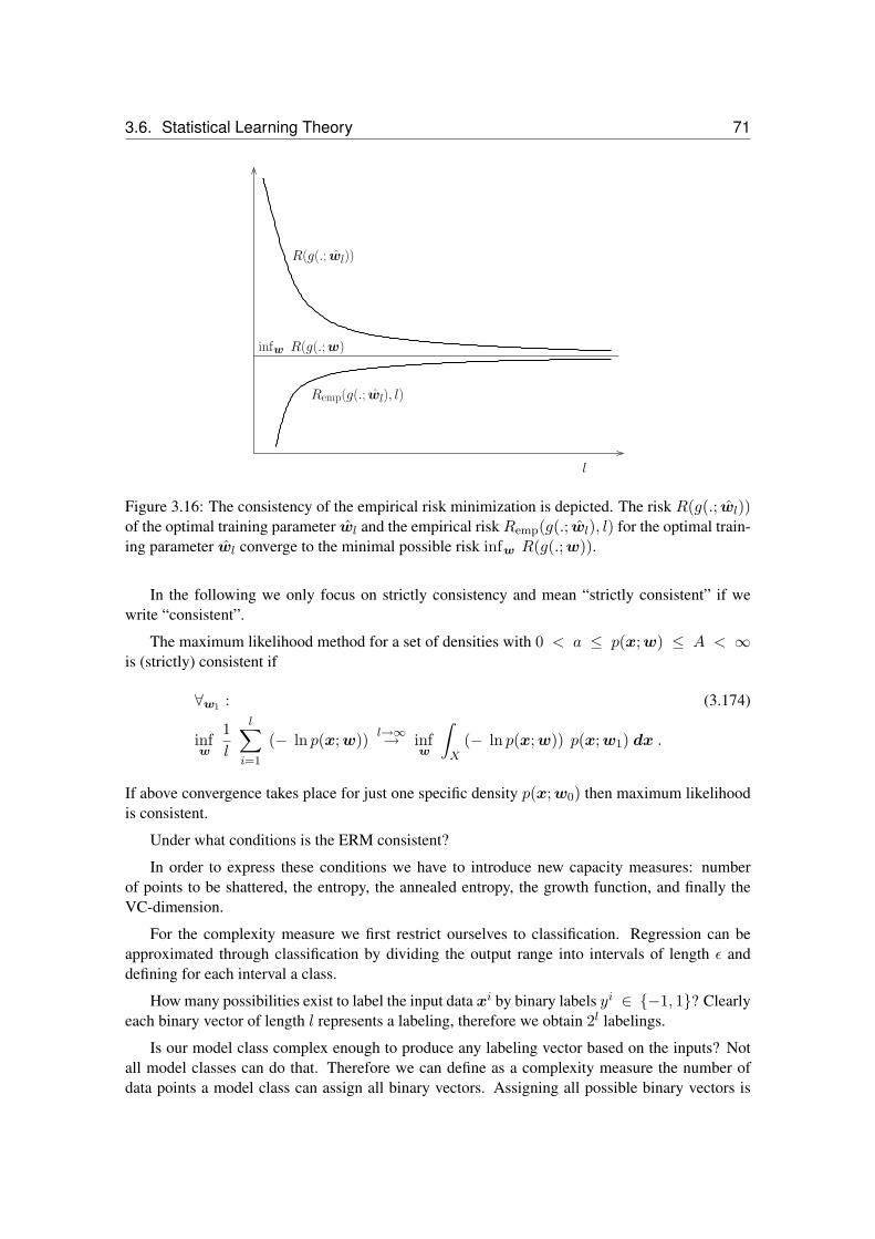
3.6. Statistical Learning Theory 71
l
R(g(.; wl))
Remp(g(.; wl), l)
infw R(g(.; w)
Figure 3.16: The consistency of the empirical risk minimization is depicted. The risk R(g(.; wl))of the optimal training parameter wl and the empirical risk Remp(g(.; wl), l) for the optimal train-ing parameter wl converge to the minimal possible risk infw R(g(.;w)).
In the following we only focus on strictly consistency and mean “strictly consistent” if wewrite “consistent”.
The maximum likelihood method for a set of densities with 0 < a ≤ p(x;w) ≤ A < ∞is (strictly) consistent if
∀w1 : (3.174)
infw
1l
l∑i=1
(− ln p(x;w)) l→∞→ infw
∫X
(− ln p(x;w)) p(x;w1) dx .
If above convergence takes place for just one specific density p(x;w0) then maximum likelihoodis consistent.
Under what conditions is the ERM consistent?
In order to express these conditions we have to introduce new capacity measures: numberof points to be shattered, the entropy, the annealed entropy, the growth function, and finally theVC-dimension.
For the complexity measure we first restrict ourselves to classification. Regression can beapproximated through classification by dividing the output range into intervals of length ε anddefining for each interval a class.
How many possibilities exist to label the input data xi by binary labels yi ∈ −1, 1? Clearlyeach binary vector of length l represents a labeling, therefore we obtain 2l labelings.
Is our model class complex enough to produce any labeling vector based on the inputs? Notall model classes can do that. Therefore we can define as a complexity measure the number ofdata points a model class can assign all binary vectors. Assigning all possible binary vectors is
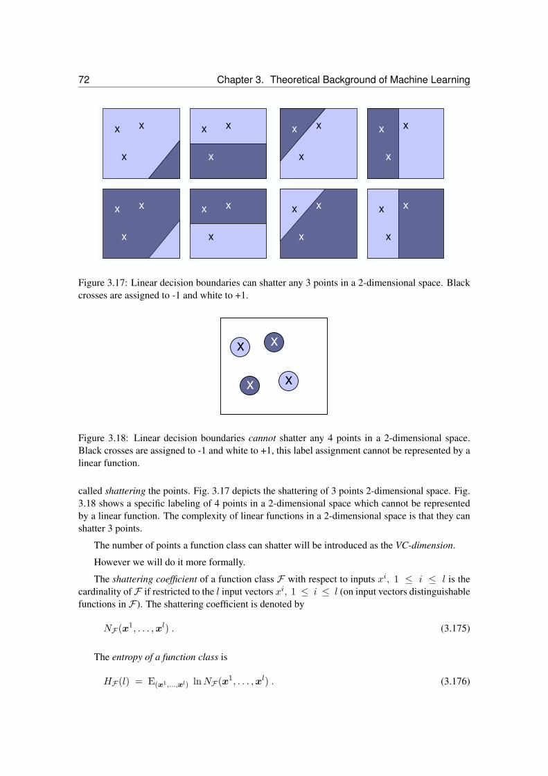
72 Chapter 3. Theoretical Background of Machine Learning
x x
x
x x
x
x
x
x x
x
x
x x
x
x x
x
x
x
x x
x
x
Figure 3.17: Linear decision boundaries can shatter any 3 points in a 2-dimensional space. Blackcrosses are assigned to -1 and white to +1.
x x
x x
Figure 3.18: Linear decision boundaries cannot shatter any 4 points in a 2-dimensional space.Black crosses are assigned to -1 and white to +1, this label assignment cannot be represented by alinear function.
called shattering the points. Fig. 3.17 depicts the shattering of 3 points 2-dimensional space. Fig.3.18 shows a specific labeling of 4 points in a 2-dimensional space which cannot be representedby a linear function. The complexity of linear functions in a 2-dimensional space is that they canshatter 3 points.
The number of points a function class can shatter will be introduced as the VC-dimension.
However we will do it more formally.
The shattering coefficient of a function class F with respect to inputs xi, 1 ≤ i ≤ l is thecardinality ofF if restricted to the l input vectors xi, 1 ≤ i ≤ l (on input vectors distinguishablefunctions in F). The shattering coefficient is denoted by
NF (x1, . . . ,xl) . (3.175)
The entropy of a function class is
HF (l) = E(x1,...,xl) lnNF (x1, . . . ,xl) . (3.176)

3.6. Statistical Learning Theory 73
The annealed entropy of a function class is
HannF (l) = ln E(x1,...,xl) NF (x1, . . . ,xl) . (3.177)
Until now we defined entropies, which are based on a probability measure on the observationsin order to have a well-defined expectation.
The next definition avoids any probability measure. The growth function of a function class is
GF (l) = ln sup(x1,...,xl)
NF (x1, . . . ,xl) . (3.178)
Note that
HF (l) ≤ HannF (l) ≤ GF (l) , (3.179)
where the first inequality comes from Jensen’s inequality and the second is obvious as the supre-mum is larger than or equal to the expectation.
Theorem 3.5 (Sufficient Condition for Consistency of ERM)If
liml→∞
HF (l)l
= 0 (3.180)
then ERM is consistent.
For the next theorem we need to define what fast rate of convergence means. Fast rate ofconvergence means exponential convergence. ERM has a fast rate of convergence if
p
(supw|R(g(.;w)) − Remp(g(.;w), l)| > ε
)< b exp
(− c ε2 l) (3.181)
holds true.
Theorem 3.6 (Sufficient Condition for Fast Rate of Convergence of ERM)If
liml→∞
HannF (l)l
= 0 (3.182)
then ERM has a fast rate of convergence.
The last two theorems were valid for a given probability measure on the observations. Theprobability measure enters the formulas via the expectation E. The growth function however doesnot use a probability measure.

74 Chapter 3. Theoretical Background of Machine Learning
Figure 3.19: The growth function is either linear or logarithmic in l.
Theorem 3.7 (Consistency of ERM for Any Probability)The condition
liml→∞
GF (l)l
= 0 (3.183)
is necessary and sufficient for the ERM to be consistent and also ensures a fast rate of convergence.
As can be seen from above theorems the growth function is very important as it is valid forarbitrary distributions of the x.
We define dVC as the largest integer for which GF (l) = l ln 2 holds:
dVC = maxll | GF (l) = l ln 2 . (3.184)
If the maximum does not exists then we set dVC = ∞. The value dVC is called the VC-dimensionof the function class F . The name VC-dimension is an abbreviation of Vapnik-Chervonenkisdimension. The VC-dimension dVC is the maximum number of vectors that can be shattered bythe function class F .
Theorem 3.8 (VC-Dimension Bounds the Growth Function)The growth function is bounded by
GF (l)
= l ln 2 if l ≤ dVC
≤ dVC
(1 + ln l
dVC
)if l > dVC
. (3.185)
Fig. 3.19 depicts the statement of this theorem, that the growth function GF (l) is either linearin l or logarithmic in l.
It follows immediately that a function class with finite VC-dimension is consistent and con-verges fast.

3.6. Statistical Learning Theory 75
However the VC-dimension allows to derive bounds on the risk as we already have shown forfunction classes with finite many functions.
We now want to give examples for the VC dimension of some function classes.
Linear functions: The VC dimension of linear discriminant functions g(x;w) = wTxis dVC = d, where d is the dimension of the input space. The VC dimension of lineardiscriminant functions g(x;w) = wTx + b with offset b is
dVC = d + 1 . (3.186)
Nondecreasing nonlinear one-dimensional functions: The VC dimension of discriminantfunctions in 1D of the form
∑ki=1
∣∣ai xi∣∣ signx + a0 is one. These functions are nonde-creasing in x, therefore they can shatter only one point: dVC = 1. The VS-dimension isindependent of number of parameters.
Nonlinear one-dimensional functions: The VC dimension of discriminant functions in 1Dof the form sin(w z) defined on [0, 2π] is infinity: dVC = ∞. This can be seen becausethere exist l points x1, . . . , xl for which a w0 exists for which sin(w0 z) is a discriminantfunction.
Neural Networks: dVC ≤ 2 W log2(e M) for multi-layer perceptions, where M are thenumber of units, W is the number of weights, e is the base of the natural logarithm (Baum& Haussler 89, Shawe-Taylor & Anthony 91). dVC ≤ 2 W log2(24 e W D) according toBartlett & Williamson (1996) for inputs restricted to [−D;D].
In the following subsections we will report error bound which can be expressed by the VC-dimension instead of the growth function, which allows to compute the actual bounds for somefunctions classes.
3.6.3 Error Bounds
The idea of deriving the error bounds is to define the set of distinguishable functions. This set hascardinality of NF , the number of different separations of inputs.
Now we can proceed as in 3.6.2.1, where we had a finite set of functions. In eq. (3.164)we replace the maximum by the sum over all functions. For finite many functions the supremumreduces to the maximum and we can proceed as in eq. (3.164) and using NF as the number offunctions in the class.
Another trick in the proof of the bounds is to use two half-samples and their difference
p
(supw
∣∣∣∣∣ 1l
l∑i=1
L(yi, g
(xi;w
)) − 1l
2l∑i=l+1
L(yi, g
(xi;w
))∣∣∣∣∣ > ε − 1l
)≥
12p
(supw
∣∣∣∣∣ 1l
l∑i=1
L(yi, g
(xi;w
)) − R(g(.;w)
∣∣∣∣∣ > ε
)

76 Chapter 3. Theoretical Background of Machine Learning
The probability that the difference of half samples exceeding a threshold is a bound on theprobability that the difference of one half-sample to the risk exceeds a threshold (“symmetriza-tion”). The symmetrization step reduced the risk which is defined on all possible samples to finitesample size. The difference on the half-samples counts how the loss on the first sample half differsfrom the second sample half.
Above considerations clarify why in the following bounds values derived from NF (finitedistinguishable functions) will appear and appear with arguments 2l (two half-samples).
Before we report the bounds, we define the minimal possible risk and its parameter:
w0 = arg minw
R(g(.;w)) (3.187)
Rmin = minw
R(g(.;w)) = R(g(.;w0)) . (3.188)
Theorem 3.9 (Error Bound)With probability of at least (1 − δ) over possible training sets with l elements, the parameter wl
(more precisely wl = w (Zl)) which minimizes the empirical risk we have
R(g(.;wl)) ≤ Remp(g(.;wl), l) +√ε(l, δ) . (3.189)
With probability of at least (1 − 2δ) the difference between the optimal risk and the risk of wl isbounded by
R(g(.;wl)) − Rmin <√ε(l, δ) +
√− ln δl
. (3.190)
Here ε(l, δ) can be defined for a specific probability as
ε(l, δ) =8l
(HannF (2l) + ln(4/δ)) (3.191)
or for any probability as
ε(l, δ) =8l
(GF (2l) + ln(4/δ)) (3.192)
where the later can be expressed though the VC-dimension dVC
ε(l, δ) =8l
(dVC (ln(2l/dVC) + 1) + ln(4/δ)) . (3.193)
The complexity measures depend all on the ratio dVCl , the VC-dimension of the class of func-
tion divided by the number of training examples.
The bound above is from [Schölkopf and Smola, 2002], whereas an older bound from Vapnikis
R(g(.;wl)) ≤ Remp(g(.;wl), l) + (3.194)
ε(l, δ)2
(1 +
√1 +
Remp(g(.;wl), l)ε(l, δ)
).

3.6. Statistical Learning Theory 77
erro
r
VC-dimension
training
complexity
bound
Figure 3.20: The error bound is the sum of the empirical error, the training error, and a com-plexity term. The complexity increases with increasing VC dimension whereas the training errordecreases with increasing complexity.
It can be seen that the complexity term decreases with 1√l. If we have zero empirical risk then
the bound on the risk decreases with 1√l.
Later in Section 4.5 we will see a bound on the expected risk which decreases with 1l for the
method of support vector machines.
The bound on the risk for the parameter wl which minimized the empirical risk has again theform
R ≤ Remp + complexity . (3.195)
This sum is depicted in Fig. 3.20, where it is also shown that the complexity term increases withthe VC-dimension whereas the empirical error decreases with increasing VC-dimension.
Note that we again arrived at a bound which is similar to the bias-variance formulation fromeq. (3.40), where the means squared error was expressed as bias term and a variance term. Biascorresponds to Remp and variance to the complexity term. With increasing complexity of a func-tion class the number of solutions with the same training error increases, that means the varianceof the solutions increases.
In many practical cases the bound is not useful because only for large number of training ex-amples l the bound gives a nontrivial value (trivial values are for example that the misclassificationrate is smaller equal 1). In Fig. 3.21 the bound is shown as being far above the actual test error.However in many practical cases the minimum of the bound is close (in terms of complexity) tothe minimum of the test error.
For regression instead of the shattering coefficient covering numbers can be used. The ε-covering number of F with respect to metric d is N (ε,F , d) which is defined as the smallestnumber which ε-cover F using metric d. Usually the metric d is the distance of the function on

78 Chapter 3. Theoretical Background of Machine Learning
erro
r
complexity
test error
training error
bound
Figure 3.21: The bound on the risk, the test error, is depicted. However the bound can be muchlarger than the test error because it is valid for any distribution of the input.
the data set X . For example the maximum norm on X , that is the distance of two functions isthe maximal difference of these two on the setX , defines the covering numberN (ε,F ,X∞) Theε-growth function is the defined as
G(ε,F , l) = ln supXN (ε,F ,X∞) . (3.196)
We obtain similar bounds on the generalization error like
R(g(.;wl)) ≤ Remp(g(.;wl), l) +√ε(ε, l, δ) , (3.197)
where
ε(ε, l, δ) =36l
(ln(12 l) + G(ε/6,F , l) − ln δ) . (3.198)
Instead to minimizing the empirical risk it would be better to minimize the risk or at least abound on them.
3.6.4 Structural Risk Minimization
The Structural Risk Minimization (SRM) principle minimizes the guaranteed risk that is a boundon the risk instead of the empirical risk alone.
In the SRM a nested set of function classes is introduced:
F1 ⊂ F2 ⊂ . . . ⊂ Fn ⊂ . . . , (3.199)

3.6. Statistical Learning Theory 79
F2 FnF1 . . .
Figure 3.22: The structural risk minimization principle is based on a structure on a set of functionswhich is nested subsets Fn of functions.
where class Fn possesses VC-dimension dnVC and
d1VC ≤ d2
VC ≤ . . . dnVC ≤ . . . , (3.200)
holds.
One realization of the SRM principle is the minimum description length [Rissanen, 1978] orminimum message length [Wallace and Boulton, 1968] principle. In the minimum descriptionlength principle a sender transmits a model and the inputs x1,x2, . . . ,xl and the receiver has torecover the labels y1, y2, . . . ,yl from the model and the inputs. If the model does not supply theexact y from the input x then the sender has also to transmit the error. Goal is to minimize thetransmission costs, i.e. the description length.
For fixed l the error is Remp and if the model complexity corresponds to the number of bits todescribe it, then the risk R is analog to the transmission cost:
transmissioncosts = Remp + complexity . (3.201)
Minimizing the transmissions costs is equivalent to minimizing the risk for appropriate error(coding the error) and appropriate model coding which defines the complexity.
If the model codes main structures in the data, then for many training examples (assume largel) the error description can be reduces. If however the model codes specific values for one or fewtraining points which may even correspond to random noise then is should not be transmitted viathe model. Transmitting the specific values through the error would be more efficient in terms ofbits than coding these values into the model. That means the model should contain rules whichapply to as many data points as possible whereas data point specific variations or noise should becontained in the error.
Is the SRM principle consistent? How fast does it converge?
The SRM is always consistent and even supplies a bound on the rate of convergence. Thatmeans the SRM procedure converges to the best possible solution with probability one as thenumber of examples l goes to infinity.
The asymptotic rate of convergence is
r(l) = |Rnmin − Rmin| +
√dnVC ln l
l, (3.202)

80 Chapter 3. Theoretical Background of Machine Learning
R
γ
Figure 3.23: Data points are contained in a sphere of radius R at the origin. A linear discriminantfunction with a boundary having distance γ to all data points is depicted.
where Rnmin is the minimal risk of the function class Fn. Asymptotic rate of convergence meansthat
p
(liml→∞
sup r−1(l)∣∣∣R(g (. ; wFnl
))− Rmin
∣∣∣ < ∞) = 1 . (3.203)
We assume that n = n(l) increases with the number of training examples so that for large
enough training examples |Rnmin − Rmin| l→∞→ 0.
If the optimal solution belongs to some class Fn then the convergence rate is
r(l) = O
(√ln ll
). (3.204)
3.6.5 Margin as Complexity Measure
The VC-dimension can be bounded by different restrictions on the class of functions. The mostfamous restriction is that the zero isoline of the discriminant function (the boundary function),provided it separates the classes properly, has maximal distance γ (this distance will later becalled “margin”) to all data points which are contained in a sphere with radiusR. Fig. 3.23 depictssuch a discriminant function. Fig. 3.24 gives an intuition why a margin reduces the number ofhyperplanes and therefore the VC-dimension.
The linear discriminant functionswTx + b can be scaled (scalingw and b) and give the sameclassification function sign
(wTx + b
). Of the class of discriminant functions leading to the same
classification function we can choose one representative.

3.6. Statistical Learning Theory 81
1/A
||w|| < A
Figure 3.24: Margin means that hyperplanes must keep outside the spheres. Therefore the possiblenumber of hyperplanes is reduced. Copyright c© 1997 [Osuna et al., 1997].
The representative is chosen with respect to the training data and is called the canonical formw.r.t. the training dataX . In the canonical form w and b are scaled that
mini=1,...,l
∣∣wTxi + b∣∣ = 1 . (3.205)
Theorem 3.10 (Margin Bounds VC-dimension)The class of classification functions sign
(wTx + b
), where the discriminant functionwTx +b is
in its canonical form versus X which is contained in a sphere of radius R, and where ‖w‖ ≤ 1γ
satisfy
dVC ≤ R2
γ2. (3.206)
This gives with the fact from eq. (3.186)
dVC ≤ min[R2
γ2
], d + 1 , (3.207)
where [.] is the floor of a real number.
Remark: The VC-dimension is defined for a model class and should not depend on trainingset.
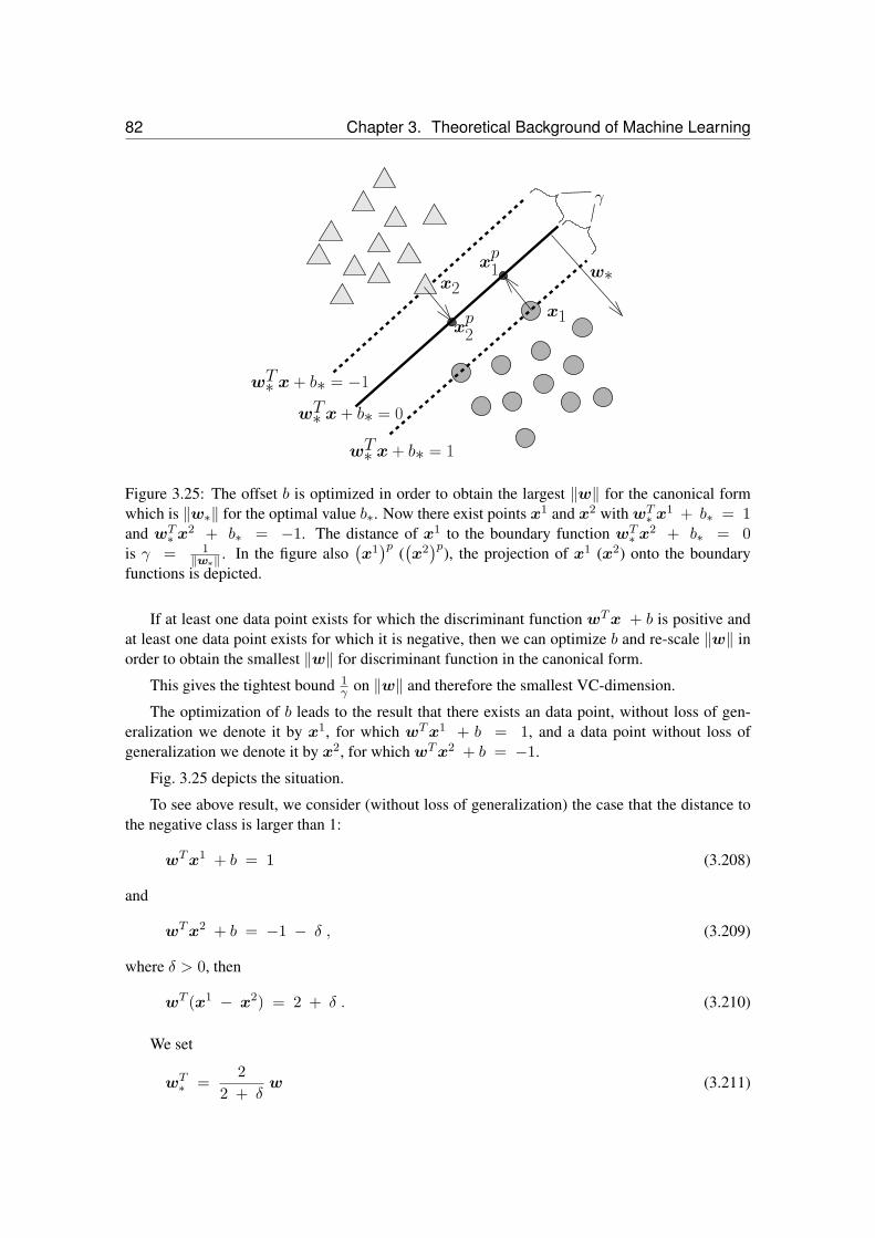
82 Chapter 3. Theoretical Background of Machine Learning
γ
x1
x2
wT∗ x + b∗ = 1
wT∗ x + b∗ = −1
w∗
xp2
wT∗ x + b∗ = 0
xp1
Figure 3.25: The offset b is optimized in order to obtain the largest ‖w‖ for the canonical formwhich is ‖w∗‖ for the optimal value b∗. Now there exist points x1 and x2 withwT∗ x1 + b∗ = 1and wT∗ x2 + b∗ = −1. The distance of x1 to the boundary function wT∗ x2 + b∗ = 0is γ = 1
‖w∗‖ . In the figure also(x1)p ((x2)p), the projection of x1 (x2) onto the boundary
functions is depicted.
If at least one data point exists for which the discriminant function wTx + b is positive andat least one data point exists for which it is negative, then we can optimize b and re-scale ‖w‖ inorder to obtain the smallest ‖w‖ for discriminant function in the canonical form.
This gives the tightest bound 1γ on ‖w‖ and therefore the smallest VC-dimension.
The optimization of b leads to the result that there exists an data point, without loss of gen-eralization we denote it by x1, for which wTx1 + b = 1, and a data point without loss ofgeneralization we denote it by x2, for which wTx2 + b = −1.
Fig. 3.25 depicts the situation.
To see above result, we consider (without loss of generalization) the case that the distance tothe negative class is larger than 1:
wTx1 + b = 1 (3.208)
and
wTx2 + b = −1 − δ , (3.209)
where δ > 0, then
wT (x1 − x2) = 2 + δ . (3.210)
We set
wT∗ =
22 + δ
w (3.211)

3.6. Statistical Learning Theory 83
which gives
‖w∗‖ < ‖w‖ . (3.212)
Further we set
b∗ = 1 − 22 + δ
wTx1 . (3.213)
We obtain
wT∗ x
1 + b∗ =2
2 + δwTx1 + 1 − 2
2 + δwTx1 = 1. (3.214)
and
wT∗ x
2 + b∗ =2
2 + δwTx2 + 1 − 2
2 + δwTx1 = (3.215)
− 22 + δ
wT(x1 − x2
)+ 1 = − 2
2 + δ(2 + δ) + 1 = − 1 .
We can generalize above example. Without loss of generalization assume that
x1 = arg minxi: yi=1
wTxi and (3.216)
x2 = arg maxxi: yi=−1
wTxi .
Then we set
wT∗ =
2wT (x1 − x2)
w (3.217)
which gives
‖w∗‖ < ‖w‖ (3.218)
because both x1 and x2 have at least a distance of 1 to the boundary functions which guaranteesthat wT (x1 − x2) > 2. Further we set
b∗ =2
wT (x1 − x2)
(− 1
2wT (x1 + x2)
)= (3.219)
− wT (x1 + x2)
wT (x1 − x2).

84 Chapter 3. Theoretical Background of Machine Learning
This gives
wT∗ x
1 + b∗ =2
wT (x1 − x2)
(wTx1 − 1
2(x1 + x2)
)= (3.220)
2wT (x1 − x2)
(12wTx1 − 1
2wTx2
)= 1
and similarly
wT∗ x
2 + b∗ = −1 . (3.221)
We see that
wT∗ (x1 − x2) = wT
∗ x1 + b∗ − wT
∗ x2 + b∗ = 2 . (3.222)
For ‖w‖ = α ‖w∗‖ with 0 < α < 1 we would obtain wT (x1 − x2) < 2 and either x1 or x2
is closer than 1 to the boundary function which contradicts that the discriminant function is in thecanonical form.
Therefore the optimal w∗ and b∗ are unique.
We want to compute the distance of x1 to the boundary function. The projection of x1 ontothe boundary function is
(x1)p = x1 − αw∗ and fulfills
wT∗(x1)p + b∗ = 0 (3.223)
⇒ wT∗(x1 − αw∗
)=
wT∗ x
1 − α ‖w∗‖2 + b∗ = 1 − α ‖w∗‖2 = 0
⇒ α =1
‖w∗‖2
⇒ (x1)p = x1 − 1
‖w∗‖2w∗
The distance of x1 to the boundary function is
∥∥x1 − (x1)p∥∥ =
∥∥∥∥x1 − x1 − 1‖w∗‖2
w∗
∥∥∥∥ =1‖w∗‖ = γ . (3.224)
Similar the distance of x2 to the boundary function is
1‖w∗‖ = γ . (3.225)

3.6. Statistical Learning Theory 85
Theorem 3.11 (Margin Error Bound)The classification functions sign
(wTx + b
)are restricted to ‖w‖ ≤ 1
γ and ‖x‖ < R. Let νbe the fraction of training examples which have a margin (distance to wTx + b = 0 ) smallerthan ρ
‖w‖ .
With probability at least of (1 − δ) of drawing l examples, the probability to misclassify anew example is bounded from above by
ν +
√c
l
(R2
ρ2 γ2ln2 l + ln(1/δ)
), (3.226)
where c is a constant.
The probability (1 − δ) is the confidence in drawing appropriate training samples whereasthe bound is on the probability of drawing a test example. The bound is from Bartlett and Shawe-Taylor.
Again the bound is of the order ν + 1√l.
In the next chapter we will introduce support vector machines as the method for structural riskminimization, where the margin is maximized.

86 Chapter 3. Theoretical Background of Machine Learning

Chapter 4
Support Vector Machines
In this chapter we focus on supervised learning with a method called “support vector machine”(SVM).
The SVM is based directly on the results from the end of previous chapter and realizes theprinciple of structural risk minimization (SRM).
SVM minimize the empirical risk simultaneously with a bound on the complexity, namely themargin.
Since the mid 90s with the papers of Cortes and Vapnik [Cortes and Vapnik, 1995] and Boser,Guyon, and Vapnik [Boser et al., 1992] and the book [Vapnik, 1995] by V. Vapnik, “Support VectorMachines” (SVMs) became very popular in the machine learning community.
Because SVMs allow for bounds on the future error, the risk, and have been proven verysuccessful in different applications they were preferred of neural networks or other supervisedlearning methods. In contrast to neural networks the SVMs have an unique solution and can besolved by a convex quadratic optimization problem.
4.1 Support Vector Machines in Bioinformatics
Machine learning methods are the best performing methods in various bioinformatics domains.
For protein 3D structure prediction support vector machines showed better performance than“threading” methods in template identification (Cheng and Baldi, 2006).
Threading was the golden standard for protein 3D structure recognition if the structure isknown (almost all structures are known).
Support vector machines were applied to the recognition of alternative splice sites and pro-vided the so far best results (Gunnar Rätsch).
Protein Homology Detection. For protein homology detection SVMs were used in differ-ent was. First, the SVM-Fisher method [Jaakkola et al., 1999, 2000] couples an iterative HMMtraining scheme with the SVM. For the same task SVMs used the mismatch-kernel [Leslie et al.,2004b,a] The mismatch kernel measures sequence similarity through amino acid identities be-tween the sequences where the frequency of almost identical subsequences is taken into account.The mismatch-kernel is related to the BLAT alignment algorithm [Kent, 2002]. The SVM-pairwisemethod according to [Liao and Noble, 2002] use as the feature vector the Smith-Waterman align-ment scores to all other training sequences. In the SW-kernel the SW-pairwise scores are used as
87

88 Chapter 4. Support Vector Machines
kernel [Vert et al., 2004] (note, that this is not a valid kernel because it is not ensured to producepositive semi-definite kernels and the SVM-optimization is not well defined). Then local align-ment (LA) kernel [Vert et al., 2004] which is similar to a local Smith-Waterman score and is basedon gap-penalties and the BLOSUM similarity matrix. Recently the oligomer based distance SVMapproach [Lingner and Meinicke, 2006] was proposed. The “HMMSTR” from [Hou et al., 2004]PSI-BLAST against SwissProt to generate a PSSM and thereafter uses a HMM and finally a SVMto classify sequences. In [Kuang et al., 2005] the mismatch kernel is generalized to process pro-files obtained by PSI-BLAST applied to the NR data base and in [Rangwala and Karypis, 2005]profiles (“position-specific scoring matrix”, PSSM) are used for local alignment-based and otherkernels in connection to the SVM.
Logan et al. [Logan et al., 2001] propose kernels which are based on motifs as are the kernelsby Ben-hur and Brutlag (2003) which use the eBLOCKS database (http://motif.stanford.edu/eblocks).
Gene Classification. Pavlidis et al. [Pavlidis et al., 2001] utilize the Fisher kernel for classify-ing genes according to the characteristics of their switching mechanisms. SVMs are successfullyused to classify co-regulated genes in yeast. Zien et al. [Zien et al., 2000] use SVMs for genefinding.
Splice Sites. Degroeve et al. [Degroeve et al., 2002] recognize the starts of introns by SVMs.
Phylogenetic. Vert [Vert, 2002c,b] uses kernels and SVMs to mark phylogenetic profiles.
Protein Classification. Hua and Sun [Hua and Sun, 2001b] classify proteins according totheir subcellular localization by SVMs.
Zavaljevski and Reifman [Zavaljevski and Reifman, 2002] apply SVMs to classify humanantibody light chains into benign or pathogenic categories.
Vert [Vert, 2002a] uses an SVMs approach to recognizing the position at which a signal peptideis cleaved from the main protein.
RNA Processing. Carter et al. [Carter et al., 2001] identified functional RNAs in genomicDNA by SVMs.
Protein Secondary Structure Prediction. For example Hua and Sun [Hua and Sun, 2001a]used SVMs instead of the typically used neural networks for protein secondary structure predic-tion.
Microarrays and Gene Expression Profiles. SVMs are used for prognosis or therapy out-come prediction based on microarray data. SVM are first used for gene selection and then againfor classification and prognosis.
The first SVM applications are by Golub et al. [Golub et al., 1999] and Mukherjee et al.[Mukherjee et al., 1999, 2000] who apply SVMs to leukemia data of the AML and ALL kind.
Pomeroy [Pomeroy et al., 2002] predicts the outcome of a therapy of embryonal brain tumorsaccording to tissue samples analyzed by microarrays. Brown et al. [Brown et al., 2000] classify ofyeast genes into functional categories based on SVMs. Moler et al. [Moler et al., 2000] use SVMsfor the recognition of colon cancer described by microarrays. Segal et al. [Segal et al., 2003]apply SVMs to the analysis of a tumor called “clear cell sarcoma”. The outcome of a breast cancerradiation or chemotherapy was predicted by van’t Veer et al. [van’t Veer et al., 2002] which wasimproved by [Hochreiter and Obermayer, 2004] by SVM-techniques. Gene expression changes

4.2. Linearly Separable Problems 89
in Drosophila embryos were investigated by Myasnikova et al. [Myasnikova et al., 2002] usingSVMs. Further publications where SVM are used to analyze microarray data include [Komuraet al., 2005, Huang and Kecman, 2005, Zhang et al., 2006, Wang et al., 2006, Tang et al., 2006,Shen and Tan, 2006].
Gene Selection form Gene Expression Profiles. Furey et al. [Furey et al., 2000] focus ongene selection for AML/ALL leukemia and colon cancer. Guyon et al. [Guyon et al., 2002]developed a method called “recursive feature elimination (RFE)” for support vector machines andapplied it to microarray data for gene selection. Su et al. [Su et al., 2003] offers a package called“RankGene” for gene ranking. In [Vert and Kanehisa, 2003] graph-driven feature extraction basedon kernel methods are proposed. The breast cancer data published in [van’t Veer et al., 2002]were overestimated because of a selection bias which comes from choosing relevant genes prior tocross-validation. This error was reported by Ambroise and McLachlan [Ambroise and McLachlan,2002] and by Tibshirani and Efron [Tibshirani and Efron, 2002].
Methylation Data. Model et al. [Model et al., 2001] use SVMs for feature selection andclassification on methylation arrays instead of cDNA microarrays.
Protein-Protein Interactions. Bock and Gough [Bock and Gough, 2001] apply SVM forprotein-protein interaction tasks.
Mass Spectrometry. In tandem mass spectrometry samples of unknown proteins are frag-mented into short sequences, called “peptides” which are measured according to mass and charge.Anderson et al. [Anderson et al., 2003] improved the determination of the peptides from databases by using SVMs.
In above Bioinformatics applications support vector machines improved previous results. There-fore SVMs are one of the standard techniques in Bioinformatics. Further applications of SVMsare given under
http://www.clopinet.com/isabelle/Projects/SVM/applist.html.
SVM web-sites with tutorials and software are
http://www.kernel-machines.org,
http://www.support-vector-machines.org/SVM_stat.html, and
http://kernelsvm.tripod.com.
4.2 Linearly Separable Problems
First we consider classification tasks which are linearly separable.
As in previous chapter we assume that objects x ∈ X from an object set X are represented ordescribed by feature vectors x ∈ Rd.
The training set consists of l objects X =x1, . . . , xl
with a label yi ∈ −1, 1 for
classification and yi ∈ R for regression. The matrix of feature vectors is X =(x1, . . . ,xl
)and
the vector of labels y =(y1, . . . , yl
)T .

90 Chapter 4. Support Vector Machines
Figure 4.1: A linearly separable problem, where data points of class 1 (the circles) are on one sideof the hyperplane (a line in two dimensions) and data points of class 2 (the triangles) are on theother side of the hyperplane.
Figure 4.2: Different solutions for linearly separating the the classes.
Linear separable means, for the training data a discriminant function wTx + b exists whichdefines a classification function sign
(wTx + b
)for which
yi = sign(wTxi + b
), 1 ≤ i ≤ l . (4.1)
That means all positive examples are of one side of the boundary functionwTx + b = 0 andall negative examples are on the other side. Fig. 4.1 shows a two-dimensional example for a linearseparable problem.
However the data can be separated by different hyperplanes as shown in Fig. 4.2 for the two-dimensional example. Which is the best separating hyperplane?
Our theoretical considerations in last chapter suggest to use the classification function with thelowest complexity. For the complexity measure we will use the margin. Fig. 4.3 gives an intuitionwhy larger margin is desirable as data points can be noise without jumping over the boundaryfunction.

4.3. Linear SVM 91
Figure 4.3: Intuitively, better generalization is expected from separation on the right hand side thanfrom the left hand side because larger distance to the data points allows for noisy data. Copyrightc© 1997 [Osuna et al., 1997].
4.3 Linear SVM
We are looking for the separating hyperplane with the largest margin, because it has the tightestbound on the VC-dimension.
The margin was defined in Section 3.6.5 as the minimal distance of the boundary functionwTx + b = 0 to all data points. As in Section 3.6.5 we assume that the classification function isdescribed by a discrimination function in the canonical form (remember that scalingw and b withthe same factor does not change the classification function), that means
mini=1,...,l
∣∣wTxi∣∣ = 1 . (4.2)
In Section 3.6.5 we saw that optimizing b in order to obtain the smallest w of vectors havingthe same directions as w leads to at least one point exists for which wTx + b = 1 and at leastone point exists for which wTx + b = −1. We then showed in Section 3.6.5 that the margin isgiven by
γ =1‖w‖ . (4.3)
The situation is depicted in Fig. 4.4.
In Section 3.6.5 we optimized b and the length ofw but not the direction ofw. We will to thisnow.
If we assume correct classification and the canonical form then
wTxi + b ≥ 1 for yi = 1 and (4.4)
wTxi + b ≤ −1 for yi = −1 . (4.5)

92 Chapter 4. Support Vector Machines
wTx + b = 1
wTx + b = −1
wTx + b = 0
w
margin γ = 1‖w‖
Figure 4.4: For the hyperplane described by the canonical discriminant function and for the opti-mal offset b (same distance to class 1 and class 2), the margin is γ = 1
‖w‖ . At least one pointexists for which wTx + b = 1 and at least one point exists for which wTx + b = −1.
The values 1 and −1 are due to the canonical form.
To maximize the margin γ, we have to maximize 1‖w‖ which means we have to minimize ‖w‖
or equivalently wTw = ‖w‖2.
To realize the structural risk minimization principle we maximize the margin but ensure correctclassification. This leads to the support vector optimization problem:
minw,b
12‖w‖2 (4.6)
s.t. wTxi + b ≥ 1 for yi = 1wTxi + b ≤ −1 for yi = −1 .
This can be rewritten as
minw,b
12‖w‖2 (4.7)
s.t. yi(wTxi + b
) ≥ 1 .
This optimization problem is well defined becausewTw = ‖w‖2 is positive definite and theconstraints are linear. The problem is a convex quadratic optimization task with has one uniquesolution.
Above formulation is in the primal space. If we use Lagrange multipliers then we can solvethis problem in the dual space.
4.3. Linear SVM 93
The Lagrange function is
L(w, b,α) =12‖w‖2 −
l∑i=1
αi(yi(wTxi + b
) − 1), (4.8)
where αi ≥ 0 are Lagrange multipliers which are larger than zero because the constraints areinequalities.
The solution of the optimization problem is a saddle point of the Lagrangian. To find thesaddle point the minimization has to be done over w and b and the maximization over αi ≥ 0.
For the minimum the derivatives of L(w, b,α) are zero:
∂L(w, b,α)∂w
= w −l∑
i=1
αi yi xi = 0 and (4.9)
∂L(w, b,α)∂b
=l∑
i=1
αi yi = 0 . (4.10)
We can solve the first equation for w and obtain
w =l∑
i=1
αi yi xi . (4.11)
And the second equation gives an equality constraint
l∑i=1
αi yi = 0 . (4.12)
The expression for w in eq. (4.11) can be substituted into the Lagrangian:
L(w, b,α) =12
(l∑
i=1
αi yi(xi)T)( l∑
i=1
αi yi xi
)− (4.13)
l∑i=1
αi yi
l∑j=1
αj yj(xj)Txi − b
l∑i=1
αi yi +
l∑i=1
αi =
12
∑i,j
αi αj yi yj
(xj)Txi −
∑i,j
αi αj yi yj
(xj)Txi +
l∑i=1
αi =
− 12
∑i,j
αi αj yi yj
(xj)Txi +
l∑i=1
αi .
The Lagrangian has to be maximized with respect to the dual variables, therefore we can minimizethe negative Lagrangian
12
∑i,j
αi αj yi yj
(xj)Txi −
l∑i=1
αi . (4.14)

94 Chapter 4. Support Vector Machines
The dual formulation is of the optimization problem is
minα
12
∑i,j
αi αj yi yj
(xj)Txi −
l∑i=1
αi (4.15)
s.t. αi ≥ 0l∑
i=1
αi yi = 0 .
The dual formulation has only box constraints and one linear equality constraint and is thereforesimpler to solve than the primal formulation.
The dual formulation in vector notation is
minα
12αTY TXTX Y α − 1Tα (4.16)
s.t. α ≥ 0
αTy = 0 ,
where Y = diag(y) is the diagonal matrix of the labels.
We can now solve the dual formulation to obtain the optimal vector α. From the primal α thedual vector w can be computed via
w =l∑
i=1
αi yi xi . (4.17)
For classification we do not need an explicit representation ofw but only the dot products betweenthe new vector x and the vectors xi:
wTx + b =l∑
i=1
αi yi(xi)Tx + b . (4.18)
The Karush-Kuhn-Tucker (KKT) conditions require that the product of Lagrange multipliersand constraint is zero for the optimal w and b:
αi(yi(wTxi + b
) − 1)
= 0 (4.19)
It follows that either
αi = 0 or (4.20)
yi(wTxi + b
)= 1 . (4.21)
The xi for which αi > 0 are called support vectors.
That means the w is only described by support vectors because the terms with αi = 0 vanish.

4.4. Linear SVM for Non-Linear Separable Problems 95
The value of b can be determined from each support xi vector because
yi(wTxi + b
)= 1 (4.22)
therefore
b = yi − wTxi . (4.23)
If the solutions α are not exact then b can be computed by averaging the computed b valuesover all support vectors.
Note that for the optimal α
b
l∑i=1
αi yi = 0 (4.24)
holds. We have for the optimal solution
wTw =l∑
i=1
αi yi wTxi = (4.25)
l∑i=1
αi yi wTxi + b
l∑i=1
αi yi −
l∑i=1
αi +l∑
i=1
αi =
l∑i=1
αi(yi(wTxi + b
) − 1)
+l∑
i=1
αi =
l∑i=1
αi ,
where we used the KKT conditions eq. (4.19).
The margin γ can be expressed by support vector weights αi for the optimal solution:
γ =1√∑li=1 αi
. (4.26)
4.4 Linear SVM for Non-Linear Separable Problems
In previous section we assumed that the classification problem is linearly separable. However inmany tasks this assumption is not true. See Fig. 4.6 for a non-linear separable task.
In Fig. 4.7 on the top line two problems are depicted which are not linearly separable. Howeverif data points can be moved then these problems are again linear separable.

96 Chapter 4. Support Vector Machines
Figure 4.5: Two examples for linear SVMs. The class of points is given by their color. Thecircled points are support vectors and the color of the regions correspond to the class points inthis region would be classified. Screen-shots from http://www.eee.metu.edu.tr/~alatan/
Courses/Demo/AppletSVM.html.
Figure 4.6: Left: linear separable task. Right: a task which is not linearly separable, where thefilled point marked with a cross is in the region of the non-filled points. Circled points are supportvectors. Copyright c© 1998 [Burges, 1998].

4.4. Linear SVM for Non-Linear Separable Problems 97
w
margin γ = 1‖w‖
ξξ
ξξξ
ξ
Figure 4.7: Two problems at the top line which are not linearly separable. If data points can bemoved then the problem would be linear separable as shown in the bottom line.

98 Chapter 4. Support Vector Machines
What does moving mean? If the data point is moved orthogonal to a separating hyperplane inthe direction of its class. With δi > 0 we can express that by(
xi)moved = xi + yi δi w (4.27)
wT(xi)moved = wTxi + yi δi ‖w‖2 (4.28)
and obtain
yi(wT
(xi)moved + b
)≥ 1 (4.29)
⇔ yi(wTxi + b
) ≥ 1 − δi ‖w‖2 . (4.30)
If we set ξi = δi ‖w‖2 then we obtain
yi(wTxi + b
) ≥ 1 − ξi . (4.31)
The new introduced variables ξi are called slack variables.
The movements expressed by the slack variables should be minimized. How strong move-ments are penalized is expressed by a new hyper-parameter C.
We obtain a optimization problem with slack variables as
minw,b,ξ
12‖w‖2 + C
l∑i=1
ξi (4.32)
s.t. yi(wTxi + b
) ≥ 1 − ξi
ξi ≥ 0 .
The Lagrange function is
L(w, b,α, ξ,µ) =12‖w‖2 + C
l∑i=1
ξi − (4.33)
l∑i=1
αi(yi(wTxi + b
) − 1 + ξi) − l∑
i=1
µi ξi ,
where αi, µi ≥ 0 are Lagrange multipliers.
At the minimum the derivatives of L(w, b,α, ξ,µ) are zero:
∂L∂w
= w −l∑
i=1
αi yi xi = 0 (4.34)
∂L∂b
=l∑
i=1
αi yi = 0 (4.35)
∂L∂ξ
= 1C − α − µ = 0 . (4.36)

4.4. Linear SVM for Non-Linear Separable Problems 99
Again be obtain
w =l∑
i=1
αi yi xi . (4.37)
and
l∑i=1
αi yi = 0 . (4.38)
Additionally, from the last derivative we obtain
αi ≤ C (4.39)
because µi ≥ 0.
The expression for w can be again substituted into the Lagrangian:
L =12
(l∑
i=1
αi yi(xi)T)( l∑
i=1
αi yi xi
)+ C
l∑i=1
ξi − (4.40)
l∑i=1
αi yi
l∑j=1
αj yj(xj)Txi − b
l∑i=1
αi yi +
l∑i=1
αi −
l∑i=1
αi ξi +l∑
i=1
αi −l∑
i=1
µi ξi =
− 12
∑i,j
αi αj yi yj
(xj)Txi +
l∑i=1
ξi (C − αi − µi) +l∑
i=1
αi =
− 12
∑i,j
αi αj yi yj
(xj)Txi +
l∑i=1
αi .
We again minimize the negative Lagrangian
12
∑i,j
αi αj yi yj
(xj)Txi −
l∑i=1
αi . (4.41)
The dual formulation is of the optimization problem with slack variables is
minα
12
∑i,j
αi αj yi yj
(xj)Txi −
l∑i=1
αi (4.42)
s.t. 0 ≤ αi ≤ Cl∑
i=1
αi yi = 0 .

100 Chapter 4. Support Vector Machines
The dual formulation with slack variables differs from the dual without slack variables in eq. (4.42)only through the upper bound C on αi.
minα
12αTY TXTX Y α − 1Tα (4.43)
s.t. 0 ≤ α ≤ C1
αTy = 0 ,
where Y = diag(y) is the diagonal matrix of the labels.
The Karush-Kuhn-Tucker (KKT) conditions require:
αi(yi(wTxi + b
) − 1 + ξi)
= 0 (4.44)
µi ξi = 0 . (4.45)
From the last equality it follows that if ξi > 0 then µi = 0. Because of the conditionC − αi − µi = 0 (derivative of Lagrangian with respect to ξi is zero) we obtain αi = C andtherefore ξi = 1 − yi
(wTxi + b
).
If µi > 0 then ξi = 0 and either yi(wTxi + b
)= 1 or αi = 0.
From αi = 0 follows that µi = C and ξi = 0 therefore
That means
αi > 0 : (4.46)
⇒ξi = yi
(wTxi + b
) − 1 > 0 and αi = Cyi(wTxi + b
)= 1 and 0 < αi < C
αi = 0 : (4.47)
⇒ ξi = 0 and yi(wTxi + b
)> 1 .
Data points which are moved (ξi > 0) have αi = C and data points on the boundary have0 < αi < C. The data points classified correctly with absolute discriminant functions valuelarger than 1 have αi = 0.
kind of data point αi ξixi moved αi = C ξi > 0xi on the boundary 0 < αi < C ξi = 0xi classified correctly αi = 0 ξi = 0
The vectors xi with αi > 0 are the support vectors. The situations is depicted in Fig. 4.8.
Again only support vectors determine the discriminant function. Data points with α = 0 donot influence the solution – even if they would be removed from the training set, the results remainsthe same.
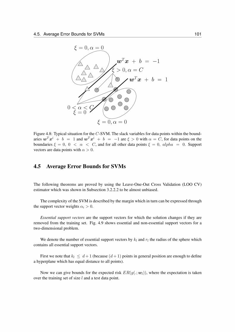
4.5. Average Error Bounds for SVMs 101
ξ > 0, α = C
ξ = 0, α = 0
ξ = 0, α = 0
0 < α < Cξ = 0
wTx + b = 1
wTx + b = −1
Figure 4.8: Typical situation for the C-SVM. The slack variables for data points within the bound-aries wTxi + b = 1 and wTxi + b = −1 are ξ > 0 with α = C, for data points on theboundaries ξ = 0, 0 < α < C, and for all other data points ξ = 0, alpha = 0. Supportvectors are data points with α > 0.
4.5 Average Error Bounds for SVMs
The following theorems are proved by using the Leave-One-Out Cross Validation (LOO CV)estimator which was shown in Subsection 3.2.2.2 to be almost unbiased.
The complexity of the SVM is described by the margin which in turn can be expressed throughthe support vector weights αi > 0.
Essential support vectors are the support vectors for which the solution changes if they areremoved from the training set. Fig. 4.9 shows essential and non-essential support vectors for atwo-dimensional problem.
We denote the number of essential support vectors by kl and rl the radius of the sphere whichcontains all essential support vectors.
First we note that kl ≤ d+ 1 (because (d+ 1) points in general position are enough to definea hyperplane which has equal distance to all points).
Now we can give bounds for the expected risk ER(g(.;wl)), where the expectation is takenover the training set of size l and a test data point.

102 Chapter 4. Support Vector Machines
w w
Figure 4.9: Essential vectors. Left: all support vectors (the circled points) are essential. Right: thethree support vectors on the right hand side line are not essential because removing one of themdoes not change the solution.
Theorem 4.1 (Average Bounds for SVMs) For the expected risk with above definitions
ER(g(.;wl)) ≤ Ekl+1
l + 1(4.48)
ER(g(.;wl)) ≤ d+ 1l + 1
(4.49)
ER(g(.;wl)) ≤E(rl+1
γl+1
)2
l + 1(4.50)
ER(g(.;wl)) ≤Emin
kl+1 ,
(rl+1
γl+1
)2
l + 1(4.51)
ER(g(.;wl)) ≤E((k∗l+1
)2∑i∗ αi∗ + m
)l + 1
(4.52)
C ≤ r−2l : ER(g(.;wl)) ≤
E(
(kl+1)2∑i αi
)l + 1
, (4.53)
where i∗ are the support vectors with 0 < αi∗ < C and m is the number of support vectors withαi = C.
All of above bounds are based on the leave-one-out cross validation estimator and its propertyto be almost unbiased.
It is important to note that we obtain for the expected risk a bound of the order 1l whereas we
saw in the theoretical sections bounds (worst case bounds) for the risk of 1√l.
Important to know would be the variance of the expected risk.

4.6. ν-SVM 103
4.6 ν-SVM
The C-support vector machine can be reformulated in a more convenient form. Instead of thehyper-parameter C another hyper-parameter ν can be introduced which has a more intuitive inter-pretation.
The hyper-parameter ν will be an upper bound on the fraction of margin errors and a lowerbound on the number of support vectors.
The primal formulation of the ν-SVM is
minw,b,ξ,ρ
12‖w‖2 − ν ρ +
1l
l∑i=1
ξi (4.54)
s.t. yi(wTxi + b
) ≥ ρ − ξi
ξi ≥ 0 and ρ ≥ 0 .
Without the slack variables the margin would be scaled by ρ. Therefore the margin is max-imized in the objective because it enters it with a negatively. However the margin can only bemaximized as long as the constraints are fulfilled.
To see the properties of this formulation we need the margin error, which is the fraction ofdata points for which
yi(wTxi + b
)< ρ . (4.55)
Theorem 4.2 (ν-SVM Properties)For the solution of the ν-SVM optimization problem eq. (4.54) holds:(i) ν is an upper bound on the fraction of margin errors.(ii) ν is a lower bound on the fraction of support vectors.(iii) Under mild conditions (see [Schölkopf and Smola, 2002]) ν asymptotically reaches the frac-tion of support vectors and the fraction of margin errors with probability 1.
The Lagrangian of the ν-SVM formulation is
L(w, b,α, ξ,µ, ρ, δ) =12‖w‖2 − ν ρ +
1l
l∑i=1
ξi − (4.56)
l∑i=1
αi(yi(wTxi + b
) − ρ + ξi) − l∑
i=1
µi ξi − δ ρ .

104 Chapter 4. Support Vector Machines
At the minimum the derivatives of L(w, b,α, ξ,µ, ρ, δ) are zero:
∂L∂w
= w −l∑
i=1
αi yi xi = 0 (4.57)
∂L∂b
=l∑
i=1
αi yi = 0 (4.58)
∂L∂ξ
=1l1 − α − µ = 0 (4.59)
∂L∂ρ
=l∑
i=1
αi − δ − ν = 0 . (4.60)
If we substitute these values into the Lagrangian we obtain
L = − 12
∑i,j
αi αj yi yj
(xj)Txi . (4.61)
The dual is
minα
12
∑i,j
αi αj yi yj
(xj)Txi (4.62)
s.t. 0 ≤ αi ≤ 1l
l∑i=1
αi yi = 0
l∑i=1
αi ≥ ν .
In contrast to the C-SVM formulation the term∑l
i=1 αi does not appear in the objectivefunction but it is lower bounded by the constant ν. This also avoids the trivial solution α = 0.
The Karush-Kuhn-Tucker (KKT) conditions require:
αi(yi(wTxi + b
) − ρ + ξi)
= 0 (4.63)
µi ξi = 0 (4.64)
δ ρ = 0 . (4.65)
The last equation together with eq. (4.60) immediately leads to the fact that for solutions withmargin larger than zero
∑li=1 αi = ν.
b and ρ can be computed from support vectors with 0 < αi <1l because then µi > 0 and
ξi = 0 therefore yi(wTxi + b
)= ρ. For two such support vectors x1 with y1 = 1 and x2

4.6. ν-SVM 105
with y2 = −1 we obtain
ρ =12(wTx1 − wTx2
)(4.66)
b = − 12(wTx1 + wTx2
)(4.67)
The first equation is obtained by adding the two equations and the second by subtracting thetwo equations. Analogously the values can be computed for more than two support vectors with0 < αi <
1l .
The constraints αi ≤ 1l ,∑l
i=1 αi = ν, and∑l
i=1 αi yi = 0 impose constraints on the ν.
First it is clear that 0 ≤ ν ≤ 1.
Let us assume that we have k < l2 examples with yi = 1 and (l − k) examples with yi = −1,
i.e. we have fewer positive examples than negative. We are now looking for the maximal ν. It isoptimal if all k positive examples have maximal value of αi = 1
l giving in sum kl . The negative
examples sum also up to kl in order to fulfill
∑li=1 αi y
i = 0. Therefore∑l
i=1 αi = 2 kl . We
obtain that
ν ≤ 2 kl. (4.68)
If k ≥ l2 , we can apply the above argumentation and obtain
ν ≤ 2 (l − k)l
. (4.69)
Merging these two cases, we obtain
ν ≤ 2 mink, (l − k)l
. (4.70)
The same holds if the number of negative examples are smaller than the positives.
Because ν is an upper bound on the fraction of margin errors, for very unbalanced data sets(small k) the ν-SVM does not allow many errors of the larger set. However for some tasks manyerrors of the larger set is the best solution.
ν-SVM may have problems with unbalanced data sets.
Next we will investigate the connection between the C-SVM and the ν-SVM.
Let us assume, that we have a ν-SVM solution with a specific ρ > 0 (ρ = 0 is excluded) andthe variables w, b, and ξ. We define new variables as
w∗ = w/ρ (4.71)
b∗ = b/ρ (4.72)
ξ∗ = ξ/ρ (4.73)

106 Chapter 4. Support Vector Machines
and we obtain as primal for the ν-SVM with the new variables:
minw∗,b∗,ξ∗,ρ
12ρ2 ‖w∗‖2 − ν ρ + ρ
1l
l∑i=1
ξ∗i (4.74)
s.t. ρ yi((w∗)Txi + b∗
) ≥ ρ − ρ ξ∗iρ ξ∗i ≥ 0 and ρ ≥ 0
that is
minw∗,b∗,ξ∗,ρ
ρ2
(12‖w∗‖2 − ν
ρ+
1l ρ
l∑i=1
ξ∗i
)(4.75)
s.t. yi((w∗)Txi + b∗
) ≥ 1 − ξ∗iξ∗i ≥ 0 and ρ ≥ 0 .
Because the variables are only rescaled, this formulation is equivalent to the original one.
If we now fix the optimal ρ of the ν-SVM solution and define C = 1l ρ then the factor ρ2 is
constant as is the additive term νρ and we obtain the C-SVM formulation:
minw∗,b∗,ξ∗
12‖w∗‖2 + C
l∑i=1
ξ∗i (4.76)
s.t. yi((w∗)Txi + b∗
) ≥ 1 − ξ∗iξ∗i ≥ 0 .
That means for each ν-SVM solution with ρ > 0 (depending on ν) there exists a C whichgives the same solution in the C-SVM formulation.
Basically the ν-SVM is more convenient for hyper-parameter selection, i.e. the selection of νcompared to the selection of C in the C-SVM. The hyper-parameter selection is also more robust.
However for unbalanced data sets the C-SVM is to prefer because only small values of ν arepossible.
4.7 Non-Linear SVM and the Kernel Trick
Until now we only considered linear models but for some problems nonlinear models are moreappropriate.
We want to apply the nice results obtained from the linear theory. The idea is to map thefeature vectors x by a nonlinear function Φ into a feature space:
Φ : Rd → RdΦ , x 7→ xφ, xφ = Φ(x) . (4.77)
In this feature space we can apply the linear theory of SVMs. Afterwards we can project theresults back into the original space. Fig. 4.10 depicts the feature mapping. In the feature space the

4.7. Non-Linear SVM and the Kernel Trick 107
Φ(x1)T Φ(x2)
Φ(x)
Φ−1
Figure 4.10: Nonlinearly separable data is mapped into a feature space where the data is linearseparable. The support vectors in feature space are marked by thicker borders. These vectors aswell as the boundary function are shown in the original space where the linear boundary functionbecomes a nonlinear boundary function.
data is assumed to be linear separable (the VC-dimension of linear functions increases with thedimensionality). The result can be transferred back into the original space.
For example consider
Φ(x) =(x2
1 , x22 ,√
2 x1 x2
). (4.78)
This is a mapping from a two-dimensional space into a three-dimensional space.
The four data points x1 = (1, 1),x2 = (1,−1),x3 = (−1, 1),x4 = (−1,−1) withlabels y1 = −1, y2 = 1, y3 = 1, y4 = −1 are not separable in the two-dimensional space.
Their images are
Φ(x1) = (1, 1,√
2)Φ(x2) = (1, 1,−
√2)
Φ(x3) = (1, 1,−√
2)Φ(x4) = (1, 1,
√2) ,
which are linearly separable in the three-dimensional space. Fig. 4.11 shows the mapping into thethree-dimensional space.
We write in the following xmn for (xm)n, the j-th component of the vector xi.
The dot product in the three-dimensional space is
ΦT (xi)Φ(xj) = x2i1 x
2j1 + x2
i2 x2j2 + 2 xi1 xi2 xj1 xj2 =
(xi1 xj1 + xi2 xj2)2 =((xi)Txj)2
.
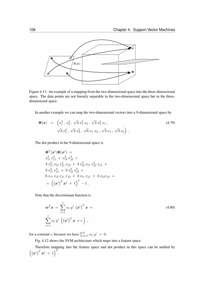
108 Chapter 4. Support Vector Machines
Φ(x)
Figure 4.11: An example of a mapping from the two-dimensional space into the three-dimensionalspace. The data points are not linearly separable in the two-dimensional space but in the three-dimensional space.
In another example we can map the two-dimensional vectors into a 9-dimensional space by
Φ(x) =(x3
1 , x32 ,√
3 x21 x2 ,
√3 x2
2 x1 , (4.79)√
3 x21 ,√
3 x22 ,√
6 x1 x2 ,√
3 x1 ,√
3 x2
).
The dot product in the 9-dimensional space is
ΦT (xi)Φ(xj) =x3i1 x
3j1 + x3
i2 x3j2 +
3 x2i1 xi2 x
2j1 xj2 + 3 x2
i2 xi1 x2j2 xj1 +
3 x2i1 x
2j1 + 3 x2
i2 x2j2 +
6 xi1 xi2 xj1 xj2 + 3 xi1 xj1 + 3 xi2xj2 =
=((xi)Txj + 1
)3 − 1 .
Note that the discriminant function is
wTx =l∑
i=1
αi yi(xi)Tx = (4.80)
l∑i=1
αi yi((xi)Tx + c
),
for a constant c, because we have∑l
i=1 αi yi = 0.
Fig. 4.12 shows the SVM architecture which maps into a feature space.
Therefore mapping into the feature space and dot product in this space can be unified by((xi)Txj + 1
)3.
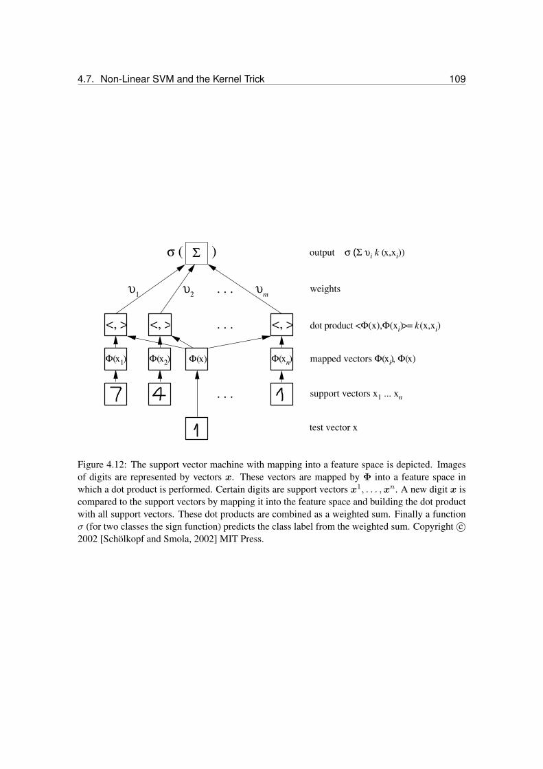
4.7. Non-Linear SVM and the Kernel Trick 109
Σ
. . .
output σ (Σ υik (x ,x
i))
w e ig h tsυ1
υ2
υm
. . .
. . .
te s t v e c tor x
s upport v e c tors x 1 ... xn
m a ppe d v e c tors Φ(xi), Φ(x )Φ(x ) Φ(x
n)
d ot prod uc t < Φ( x ),Φ( xi)>= k( x ,x
i)< , > < , > < , >
Φ(x 1) Φ(x 2)
σ ( )
Figure 4.12: The support vector machine with mapping into a feature space is depicted. Imagesof digits are represented by vectors x. These vectors are mapped by Φ into a feature space inwhich a dot product is performed. Certain digits are support vectors x1, . . . ,xn. A new digit x iscompared to the support vectors by mapping it into the feature space and building the dot productwith all support vectors. These dot products are combined as a weighted sum. Finally a functionσ (for two classes the sign function) predicts the class label from the weighted sum. Copyright c©2002 [Schölkopf and Smola, 2002] MIT Press.

110 Chapter 4. Support Vector Machines
A function which produces a scalar out of two vectors is called kernel k. In our example we
have k(xi,xj
)=((xi)Txj + 1
)3.
Certain kernels represent the mapping of vectors into a feature space and a dot product in thisspace.
The following theorem characterizes functions which build a dot product in some space.
Theorem 4.3 (Mercer)Let the kernel k be symmetric and from L2(X ×X) defining a Hilbert-Schmidt operator
Tk(f)(x) =∫Xk(x,x′) f(x′) dx′ . (4.81)
If Tk is positive semi-definite, i.e. for all f ∈ L2(X)∫X×X
k(x,x′) f(x) f(x′) dx dx′ ≥ 0 , (4.82)
then Tk has eigenvalues λj ≥ 0 with associated eigenfunctions ψj ∈ L2(X). Further
(λ1, λ2, . . .) ∈ `1 (4.83)
k(x,x′) =∑j
λj ψj(x) ψj(x′) , (4.84)
where `1 is the space of vectors with finite one-norm and the last sum converges absolutely anduniformly for almost all x and x′.
The sum may be an infinite sum for which the eigenvalues converge to zero. In this case thefeature space is an infinite dimensional space.
Here “for almost all” means “except for a set with zero measure”, i.e. single points may leadto an absolute and uniform convergence. That the convergence is “absolutely and uniformly” isimportant because the sum can be resorted and derivative and sum can be exchanged.
Note that if X is a compact interval [a, b] and k is continuous then eq. (4.82) is equivalent topositive definiteness of k. A kernel k is positive semi-definite if for all l, all x1, . . . ,xl, and allαi, 1 ≤ i ≤ l
l,l∑i,j=1,1
αi αj k(xi,xj) ≥ 0 . (4.85)
We define the Gram matrixK as Kij = k(xi,xj) the above inequality is
αTK α ≥ 0 , (4.86)
which means that the Gram matrix has non-negative eigenvalues, i.e. is positive semi-definite.

4.7. Non-Linear SVM and the Kernel Trick 111
The mapping Φ can be explicitly given as
Φ(x) =(√
λ1 ψ1(x),√λ2 ψ2(x), . . .
)(4.87)
Note that Φ(x) ∈ `2, where `2 is the set of all vectors which have finite Euclidean norm.
From the fact that the sum in the theorem converges uniformly it follows that for every εthere exists a N(ε) so that the first N(ε) components of Φ(x) are sufficient to approximate thekernel with error smaller than ε. That means infinite dimensional feature spaces can always beapproximated by finite feature space of accuracy ε.
We express the parameter vector w by a linear weighed sum of support vectors. That meansw lives in a subspace of dimension equal or smaller than l, the number of training examples.
If new vectors contain directions orthogonal to the space spanned by the training vectors thenthese directions are ignored by the classification function.
Note that in general the points in feature space are on a manifold, like a folded sheet of paper inthe three-dimensional space. On the other hand the margin in computed in the full space. Here themargin as complexity measure may be questionable because functions are distinguished at regionsin space where no data point can appear. The same holds if the original space because featuresmay have dependencies between each other.
The C-SVM with slack variables in its dual form from eq. (4.42) is only expressed by dotproducts. It can be written in with kernels in the feature space by just replacing
(xi)Txj by
k(xi,xj). This is called the kernel trick. In any algorithm which is based only on dot productsa non-linear algorithm can be constructed by introducing the kernel at the places where the dotproducts where before.
Applying the kernel trick, the problem in eq. (4.42 is now
minα
12
∑i,j
αi yi αj y
j k(xi,xj) −l∑
i=1
αi (4.88)
s.t. 0 ≤ αi ≤ Cl∑
i=1
αi yi = 0 .
The discriminant function from eq. (4.18) can be formulated using a kernel as
wTx + b =l∑
i=1
αi yi k(xi,x) + b . (4.89)

112 Chapter 4. Support Vector Machines
The most popular kernels are the following:
linear kernel: k(xi,xj) =(xi)Txj (4.90)
RBF kernel: k(xi,xj) = exp(− ‖x
i − xj‖22 σ2
)(4.91)
polynomial kernel: k(xi,xj) =((xi)Txj + β
)α(4.92)
sigmoid kernel: k(xi,xj) = tanh(α(xi)Txj + β
)(4.93)
Comments:
The sigmoid kernel is not positive semi-definite for all α and β and is not a very popularchoice.
The RBF kernel is the most popular choice.
The RBF kernel maps to feature vectors of length 1, because k(x,x) = ΦT (x)Φ(x) = 1.Therefore the RBF kernel maps onto a hyper-sphere. Because k(x1,x2) > 0 all vectors arein the same octant in the feature space. The kernel basically measures the angle between thevectors.
The Gram matrix of the RBF kernel has full rank if training examples are distinct fromeach other. Thus SVMs with RBF kernels have infinite VC-dimension. Fig. 4.13 depicts thesituation that an RBF-kernel is sitting on top of each data point, therefore all training pointscan be separated.
The space of an RBF kernel is infinite. However the eigenvalues of the Hilbert-Schmidtoperator decay exponentially with their number λn+1 ≤ C exp
(− c σ n1/d)
(Schaback& Wendland, 2002 – C and c are constants independent of n) for a bounded domain inRd. Thus, σ controls the decay of the eigenvalues and therefore the dimensions of the finitedimensional space for which the kernel can be approximated ε-exact with a dot product.Basically σ controls the dimension of the feature space approximation.
Sums and limits of positive semi-definite (p.d.) kernels are also positive semi-definite ker-nels. If k1 and k2 are p.d. kernels then also k(x1,x2) =
∫X k1(x1,x) k1(x2,x) dx and
k(x1,x2) = k1(x1,x2) k2(x1,x2).
Fig. 4.16 shows again the example from Fig. 4.6 but now with a polynomial kernel of degree3. The non-linear separable problem can be separated.
The figures 4.18, 4.19, and 4.20 give SVM examples for the RBF kernel and for the polynomialkernels.
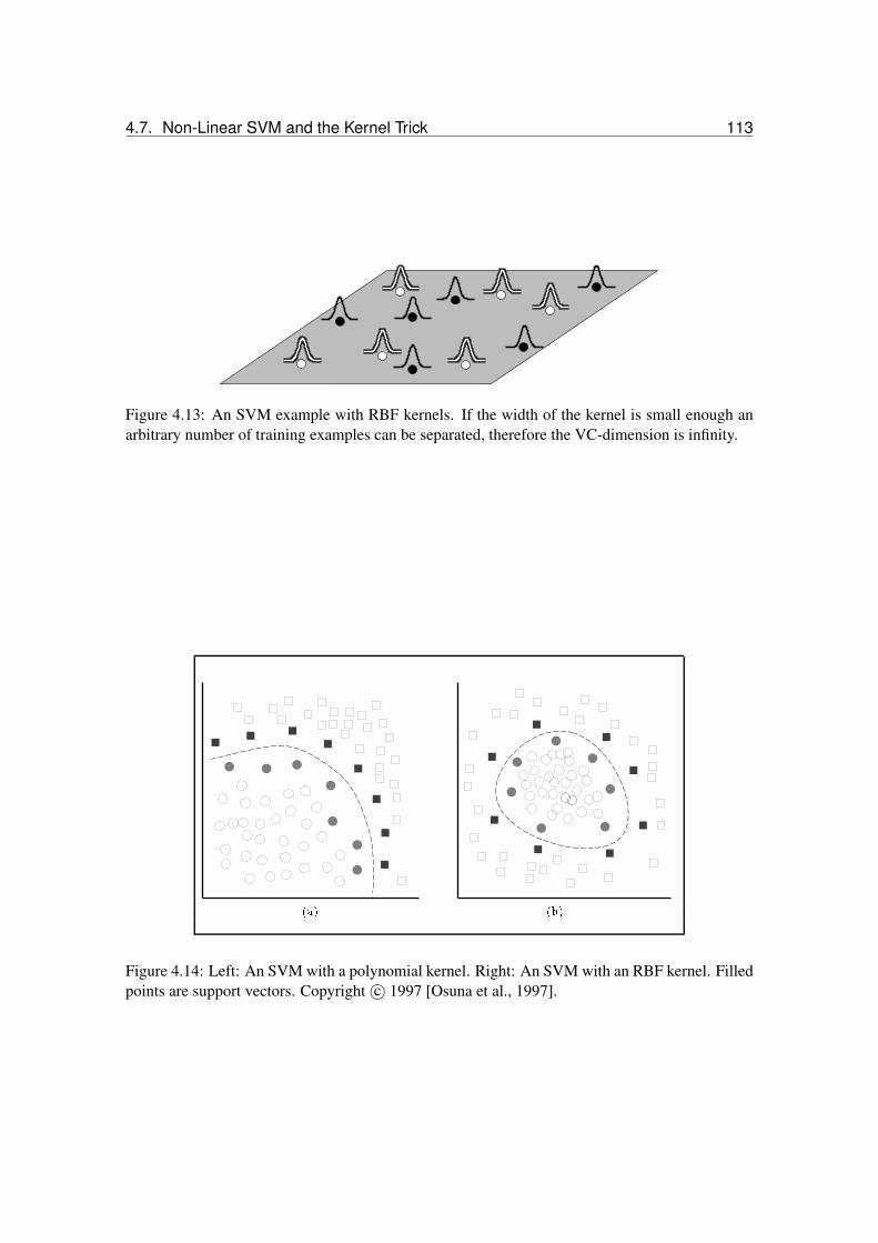
4.7. Non-Linear SVM and the Kernel Trick 113
Figure 4.13: An SVM example with RBF kernels. If the width of the kernel is small enough anarbitrary number of training examples can be separated, therefore the VC-dimension is infinity.
Figure 4.14: Left: An SVM with a polynomial kernel. Right: An SVM with an RBF kernel. Filledpoints are support vectors. Copyright c© 1997 [Osuna et al., 1997].

114 Chapter 4. Support Vector Machines
Figure 4.15: SVM classification with an RBF kernel. Support vectors are circled.Copyrightc©2002 [Schölkopf and Smola, 2002] MIT Press.
Figure 4.16: The example from Fig. 4.6 but now with polynomial kernel of degree 3. The righttask can now be separated. Copyright c© 1998 [Burges, 1998].

4.7. Non-Linear SVM and the Kernel Trick 115
Figure 4.17: SVM with RBF-kernel. Left: small σ. Right: larger σ. The class of points is givenby their color. The circled points are support vectors and the color of the regions correspond to theclass points in this region would be classified. Screen-shots from http://www.eee.metu.edu.
tr/~alatan/Courses/Demo/AppletSVM.html.

116 Chapter 4. Support Vector Machines
Figure 4.18: SVM with RBF kernel with different σ. From the upper left to the lowerright σ = 0.3, 0.18, 0.16, 0.14, 0.12, 0.1. Screen shots from http://www.csie.ntu.edu.tw/
~cjlin/libsvm/.

4.7. Non-Linear SVM and the Kernel Trick 117
Figure 4.19: SVM with polynomial kernel with different degrees α. From the upper left tothe lower right α = 2, 3, 4, 8. Screen-shots from http://www.csie.ntu.edu.tw/~cjlin/
libsvm/.
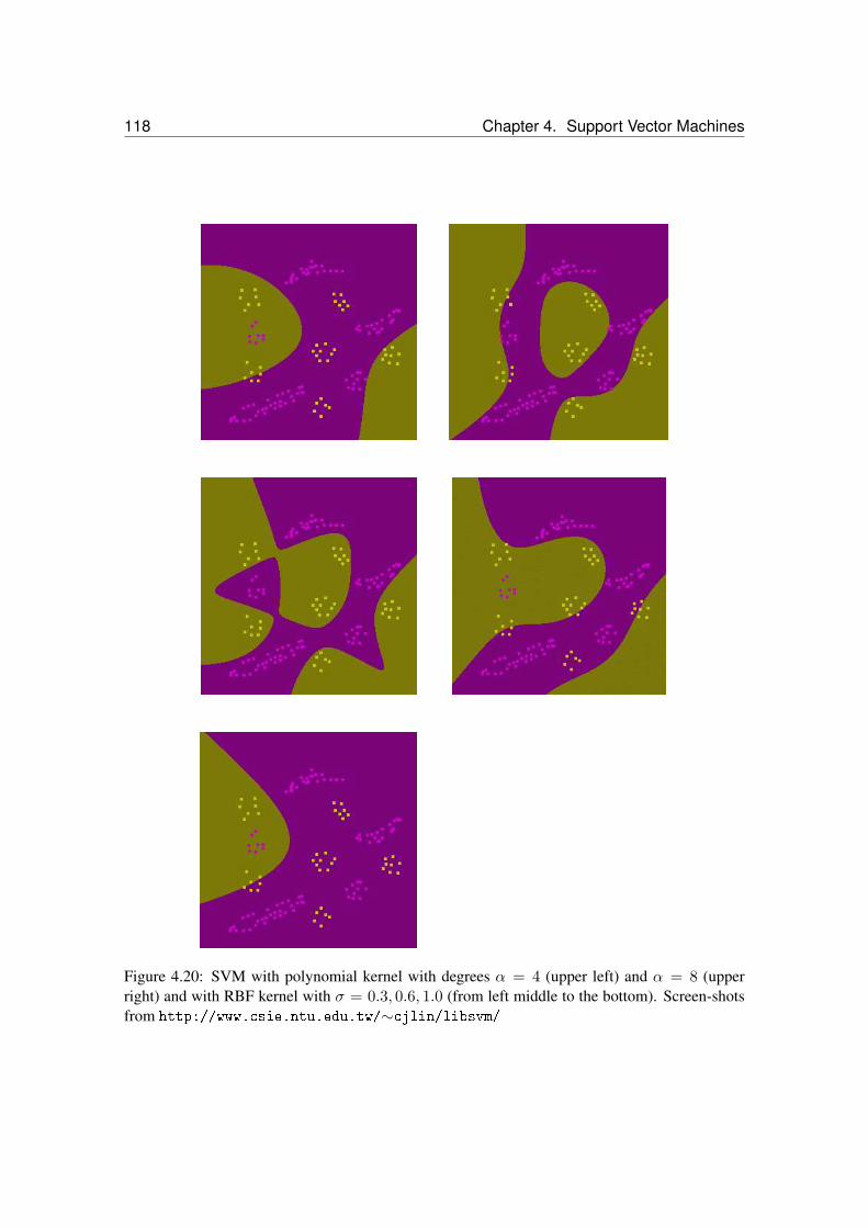
118 Chapter 4. Support Vector Machines
Figure 4.20: SVM with polynomial kernel with degrees α = 4 (upper left) and α = 8 (upperright) and with RBF kernel with σ = 0.3, 0.6, 1.0 (from left middle to the bottom). Screen-shotsfrom http://www.csie.ntu.edu.tw/∼cjlin/libsvm/
4.8. Other Interpretation of the Kernel: Reproducing Kernel Hilbert Space 119
4.8 Other Interpretation of the Kernel: Reproducing Kernel HilbertSpace
Basicly, this section is from Wikipedia, the free encyclopedia, http://en.wikipedia.org/wiki/Reproducing_kernel_Hilbert_space.
Hilbert spaces can be defined by reproducing kernels (Nachman Aronszajn and, independently,Stefan Bergman in 1950).
Let X be an arbitrary set and H a Hilbert space of complex-valued functions on X . We saythat H is a reproducing kernel Hilbert space if every linear map of the form
Lx : f 7→ f(x) (4.94)
from H to the complex numbers is continuous for any x in X . That is the evaluation at x.
Theorem 4.4 (Riesz representation theorem) LetH∗ denoteHÂt’s dual space, consisting of allcontinuous linear functionals from H into the field C. If x is an element of H , then the functionφx defined by
φx(y) = 〈y,x〉 ∀y ∈ H , (4.95)
where 〈·, ·〉 denotes the inner product of the Hilbert space, is an element of H∗.
Every element of H∗ can be written uniquely in this form, that is the mapping
Φ : H → H∗, Φ(x) = φx (4.96)
is an isometric (anti-) isomorphism.
This theorem implies that for every x in X there exists an element Kx of H with the propertythat:
f(x) = 〈f, Kx〉 ∀f ∈ H (∗). (4.97)
The function Kx is called the point-evaluation functional at the point x.
Since H is a space of functions, the element Kx is itself a function and can therefore beevaluated at every point. We define the function K : X ×X → C by
K(x,y) def= Kx(y). (4.98)
This function is called the reproducing kernel for the Hilbert space H and it is determinedentirely by H because the Riesz representation theorem guarantees, for every x in X , that theelement Kx satisfying (*) is unique.
Properties:

120 Chapter 4. Support Vector Machines
The reproducing property
It holds that
〈K(x, ·),K(y, ·)〉 = K(x,y). (4.99)
Orthonormal sequences
If φk∞k=1 is an orthonormal sequence such that the closure of its span is equal to H , then
K (x,y) =∞∑k=1
φk (x)φk (y) . (4.100)
The next theorem from Moore-Aronszajn states that every symmetric, positive definite kerneldefines a unique reproducing kernel Hilbert space.
Theorem 4.5 (Moore-Aronszajn) Suppose K is a symmetric, positive definite kernel on a set E.Then there is a unique Hilbert space of functions on E for which K is a reproducing kernel.
Proof. Define, for all x in E, Kx = K(x, ·). Let H0 be the linear span of Kx : x ∈ E.Define an inner product on H0 by⟨
n∑j=1
bj Kyj ,
l∑i=1
αi Kxi
⟩=
m∑i=1
n∑j=1
αi βj K(yj ,xi). (4.101)
The symmetry of this inner product follows from the symmetry of K and the non-degeneracyfollows from the fact that K is positive definite.
LetH be the completion ofH0 with respect to this inner product. ThenH consists of functionsof the form
f(x) =∞∑i=1
αi Kxi(x) (4.102)
where∑∞
i=1 α2i K(xi,xi) < ∞. The fact that the above sum converges for every x follows
from the Cauchy-Schwartz inequality.
Now we can check the RKHS property, (*):
〈f,Kx〉 =
⟨ ∞∑i=1
αi Kxi ,Kx
⟩=∞∑i=1
αi K(xi,x) = f(x). (4.103)

4.9. Example: Face Recognition 121
To prove uniqueness, let G be another Hilbert space of functions for which K is a reproducingkernel. For any x and y in E, (*) implies that 〈Kx,Ky〉H = K(x,y) = 〈Kx,Ky〉G. By linearity,〈·, ·〉H = 〈·, ·〉G on the span of Kx : x ∈ E. ThenG = H by the uniqueness of the completion.
References:
Nachman Aronszajn, Theory of Reproducing Kernels, Transactions of the American Math-ematical Society, volume 68, number 3, pages 337ÂU404, 1950.
Alain Berlinet and Christine Thomas, Reproducing kernel Hilbert spaces in Probability andStatistics, Kluwer Academic Publishers, 2004.
George Kimeldorf and Grace Wahba, Some results on Tchebycheffian Spline Functions, J.Mathematical Analysis and Applications, 33, 1 (1971) 82ÂU95.
Grace Wahba, Spline Models for Observational Data, SIAM, 1990.
Felipe Cucker and Steve Smale, On the Mathematical Foundations of Learning, Bulletin ofthe American Mathematical Society, volume 39, number 1, pages 1ÂU49, 2002.
4.9 Example: Face Recognition
The following example is extracted from [Osuna et al., 1997].
An SVM is trained on a database of face and non-face images of size 19× 19 pixel. As kernela polynomial kernel with α = 2 and for the SVM parameter C = 200 are used.
The data is preprocessed:
Pixels close to the boundary of the window are removed to reduce background patterns.
To correct of an illumination gradient, a best-fit brightness plane is subtracted from thewindow pixel values (reduction of light and heavy shadows).
A histogram equalization is performed over the patterns in order to compensate for differ-ences in illumination brightness, different camera response curves, etc.
Negative pattern (images without a face) were images of landscapes, trees, buildings, rocks,etc.
The system was used in a bootstrapping setting: misclassifications of the first system wereused for a second system as negative examples. In this was difficult examples were filtered out tobe recognized by a more specialized system.
The following steps were used to produce an output:
Re-scaling of the input image several times.
Cutting of 19× 19 window patterns out of the scaled image.
Preprocessing of the window using a mask, light correction and histogram equalization.

122 Chapter 4. Support Vector Machines
NON-FACES
FACES
Figure 4.21: Face recognition example. A visualization how the SVM separates faces from non-faces. Support vectors are images of certain faces and images of which are close to face images.The fact that most support vectors are non-faces is depicted in the figure. Copyright c© 1997[Osuna et al., 1997].
Classification of the pattern using the SVM.
If the SVM predicts a face, drawing a rectangle around the face in the output image.
Fig. 4.21 depicts how faces should be separated from non-faces using a SVM. More non-facesare used as support vectors because they form the majority class.
Figures 4.22, 4.23, 4.24, 4.25, 4.26, and 4.27 show the result of the face extraction experiment.Figures 4.26 and 4.27 show more difficult tasks where people are not looking into the camera andfalse positives and false negatives are present.
4.10 Multi-Class SVM
The theory of SVMs has been developed for two classes, i.e. for binary classification. Howeverin real world applications more than one class is available. For example in classifying of proteins

4.10. Multi-Class SVM 123
Figure 4.22: Face recognition example. Faces extracted from an image of the Argentina soccerteam, an image of a scientist, and the images of a Star Trek crew (even the Klingon face wasfound!). Copyright c© 1997 [Osuna et al., 1997].

124 Chapter 4. Support Vector Machines
Figure 4.23: Face recognition example. Faces are extracted from an image of the German soccerteam and two lab images. Copyright c© 1997 [Osuna et al., 1997].

4.10. Multi-Class SVM 125
Figure 4.24: Face recognition example. Faces are extracted from another image of a soccer teamand two images with lab members. Copyright c©1997 [Osuna et al., 1997].

126 Chapter 4. Support Vector Machines
Figure 4.25: Face recognition example. Faces are extracted from different view and differentexpressions. Copyright c© 1997 [Osuna et al., 1997].

4.10. Multi-Class SVM 127
Figure 4.26: Face recognition example. Again faces are extracted from an image of a soccer teambut the players are moving during taking the image. Clearly false positives and false negatives arepresent. Copyright c© 1997 [Osuna et al., 1997].

128 Chapter 4. Support Vector Machines
Figure 4.27: Face recognition example. Faces are extracted from a photo of cheerleaders. Herefalse positives are present. Copyright c© 1997 [Osuna et al., 1997].
into structural classes (e.g. according to SCOP) there are many structural classes.
One-against the rest. The first approach to using SVMs to multi-class problems ofM classesis to construct for every class j a binary classifier which separates the class from the rest. Weassume that a data point belongs exactly to one class.
Given the discriminant functions gj of these classifiers we can chose the
arg maxj=1,...,M
gj(x) = arg maxj=1,...,M
l∑i=1
yij αij k(x,xi
)+ bj , (4.104)
where yij = 1 if xi belongs to class j and otherwise yij = −1, αij and bj are the optimal param-eters of the “j-th class against the rest” SVM classification problem. This is a “winner-takes-all”approach.
For this approach confusion can exist if two classes have a boundary region where only dataof these two classes are located. The classifier is chosen to optimize all data and therefore specialparameters for discriminating these two classes are not optimal. In the next approach all pairwiseclassifiers are considered.
Pairwise Classifiers. Another approach to multi-class SVM is to train (optimize) an SVM forevery pair of classes which separates only these two classes. This gives M (M−1)
2 classificationtasks.
Note that the single tasks are computationally not as expensive as the one-against-the-restbecause the training set is reduced.
A new data point is assigned to the class which obtained the highest number of votes. A classobtains a vote if a pairwise classifier predicts the class. For large M the procedure can be made

4.11. Support Vector Regression 129
more efficient because not all classifiers must be evaluated: the classes which cannot obtain moreor equal as many votes as the best class can be excluded.
Intuitively, for very similar classes a new pattern belonging to these classes results in (M − 2)votes for each these classes and the decision is determined by the pairwise classifier of these twoclasses.
This is the our preferred multi-class approach because in practical problems it often outper-formed the other approaches. Let now yi ∈ 1, . . . ,M give directly the class xi belongs to.
Multi-class Objectives. The direct optimization of the multi-class classification problem ispossible via
minwj ,bj ,ξj
12
M∑j=1
‖wj‖2 + Cl∑
i=1
∑j 6=yi
ξij (4.105)
s.t. wTyix
i + byi ≥ wTj x
i + bj + 2 − ξij
ξij ≥ 0 ,
for all i = 1, . . . , l and all j = 1, . . . ,M such that j 6= yi.
The training is more complex here because all variables and data points are treated in oneoptimization problem. The performance is about the performance of the one-against-the-rest ap-proach.
Comments. Sometimes classification can be made more robust by prediction additional fea-tures of the data points. For example proteins can be classified into pure helical or pure beta-sheetstructures, or the surface accessibility, polarity, atomic weight, hydrophobicity etc. can be pre-dicted. For discrimination of similar classes these additional information might be helpful. It issimilar to “error-correcting output coding”, where additional bits help to correct the binary string.
4.11 Support Vector Regression
Now we want to apply the support vector technique to regression, i.e. the task is not to classifythe example x by assigning a binary label but to assign a real value. That means y is now a realnumber y ∈ R.
But how can regression derived from classification? Ideas from statistical learning theorycarry over to regression: a function class is the class which approximates functions with precisionε. The class complexity depends now also on ε. Also leave-one-out estimates are possible is onlyfew vectors (the support vectors) are used to define the regression function.
If y ∈ I and I is a compact subset of R – for simplicity we assume that I is connected, i.e.a interval in R – then I can be covered by finite many compact intervals of length ε > 0. Eachof these intervals defines a class. Even more convenient would be that we use only the intervalboundaries and classify whether a data point is larger or smaller than the boundary. In this case alinear regression function can be represented through a linear classification task with ε precision.
Therefore regression can be transformed into a classification task with ε > 0 precision. Reduc-ing the precision allows to described the regression function with few vectors because all zero-loss

130 Chapter 4. Support Vector Machines
52 B. Scho lk o p f a n d A .J . Sm o la
x
x
xx
x
x
xx
x
x
x
x
x
x
+ε− ε
x
ξ+ε
− ε0
ξ
Figure 4.28: Support vector regression. A regression function is found such that a tube with radiusε around the regression function contains most data. Points outside the tube are penalized by ξ.Those penalties are traded off against the complexity given by ‖w‖, which is represented by theslope of a linear function. Copyright c© 2002 [Schölkopf and Smola, 2002] MIT Press.
data points do not contribute to the optimal regression function. Support vectors would be at theborder of the intervals and outliers, which are data points differing more than ε from their neigh-bors which are equal to one another. However this formulation would be dependent on the choiceof the intervals. If the intervals are shifted then permanent support vectors are only the outliers.
To define these permanent support vectors we need the notion of ε-insensitive loss function
|y − g(x)|ε = max0 , |y − g(x)| − ε , (4.106)
where ε > 0. This loss function was introduced by [Vapnik, 1995].
If we now consider again linear functions wTx + b then we obtain the situation depicted inFig. 4.28. The errors must be distinguished as being more than ε below the target y or more thanε above the target y and are defined as
ξ− = max0 , g(x) − y − ε (4.107)
ξ+ = max0 , y − g(x) − εξ =
(ξ− + ξ+
)where again only xi with ξi > 0 are support vectors.
The complexity is again defined through ‖w‖2. However the motivation through a maximalmargin is no longer valid.
Small ‖w‖2 means a flat function, e.g. in the linear case a small slope.
More interesting small ‖w‖2 means small variation around the constant b of the regressionfunction on a compact set of feature vectors x. On the compact set ‖x‖ ≤ R holds. We obtainwith the Cauchy-Schwarz inequality∥∥wTx
∥∥ ≤ ‖w‖ ‖x‖ ≤ ‖w‖ R . (4.108)

4.11. Support Vector Regression 131
xx
xx
x
xx
x xx
xxx
xxx
xx
xx
x
x
xy α+
= C
α− = C
x
+ε0−ε
Figure 4.29: Nonlinear support vector regression is depicted. A regression function is found suchthat a tube with radius ε around the regression function contains most data.
This holds also for the kernel version which means for g(x) =∑l
i=1 αi yi k(x,xi) + b:
‖g(x) − b‖ ≤ ‖w‖ R ≤√∑
i,j
αi αj k(xi,xj) R ≤ (4.109)
‖α‖ √emax R ,
where emax is the maximal eigenvalue of the kernel matrix, i.e. the Gram matrix.
We obtain as optimization problem
minw,b,ξ+,ξ−
12‖w‖2 +
C
l
l∑i=1
(ξ+i + ξ−i
)(4.110)
s.t. yi − (wTxi + b
) ≤ ε + ξ+i(
wTxi + b) − yi ≤ ε + ξ−i
ξ+i ≥ 0 and ξ−i ≥ 0 .
The Lagrangian is
L(w, b, ξ+, ξ−,α+,α−,µ+,µ−
)= (4.111)
12‖w‖2 +
C
l
l∑i=1
(ξ+i + ξ−i
) − l∑i=1
(µ+i ξ
+i + µ−i ξ
−i
) −l∑
i=1
α+i
(ε + ξ+
i − yi + wTxi + b) −
l∑i=1
α−i(ε + ξ−i + yi − wTxi − b
),
where α+,α−,µ+,µ− ≥ 0.

132 Chapter 4. Support Vector Machines
The saddle point conditions require
∂L
∂b=
l∑i=1
(α+i − α−i
)= 0 (4.112)
∂L
∂w= w −
l∑i=1
(α+i − α−i
)xi = 0
∂L
∂ξ+=
C
l1 − α+ − µ+ = 0
∂L
∂ξ−=
C
l1 − α− − µ− = 0
The last two equations constrain the α+i and α−i whereas the first two equations can be inserted
into the Lagrangian to eliminate the primal variables.
We obtain as dual formulation
minα+,α−
12
(l,l)∑i,j=(1,1)
(α+i − α−i
) (α+j − α−j
) (xi)Txj + (4.113)
ε
l∑i=1
(α+i + α−i
) − l∑i=1
yi(α+i − α−i
)s.t. 0 ≤ α+
i ≤C
l
0 ≤ α−i ≤C
ll∑
i=1
(α+i − α−i
)= 0 .
The regression function can be written as
g(x) =l∑
i=1
(α+i − α−i
) (xi)Tx + b . (4.114)
The KKT conditions state for the optimal parameters:
α+i
(ε + ξ+
i − yi + wTxi + b)
= 0 (4.115)
α−i(ε + ξ−i + yi − wTxi − b
)= 0
ξ+i µ+
i = 0ξ−i µ−i = 0 .

4.11. Support Vector Regression 133
From ξ+i > 0 follows that µ+
i = 0 and therefore α+i = C
l . The analog holds for ξ−i , µ−i
and α−i . We obtain as conditions
ξ+i
(C
l− α+
i
)= 0 (4.116)
ξ−i
(C
l− α−i
)= 0 .
The data points xi with α+i = C
l are outside the ε-tube.
Data points with 0 < α+i < C
l are on the ε-tube border (same for 0 < α−i < Cl ). Because
α+i < C
l implies µ+i > 0 and therefore ξ+
i = 0. But 0 < α+i implies ε+ ξ+
i − yi +wTxi + b =0 that is ε + − yi + wTxi + b = 0 from which b can be computed as
b = yi − wTxi − ε . (4.117)
And for 0 < α−i < Cl the value b can be computed through
b = yi − wTxi + ε . (4.118)
If α+i > 0 and α−i > 0, then
ε + ξ+i − yi + wTxi + b = 0 and (4.119)
ε + ξ−i + yi − wTxi − b = 0 .
and adding both equations gives
2 ε + ξ+i + ξ−i = 0 (4.120)
which contradicts ε > 0.
Therefore we have
α+i α−i = 0 . (4.121)
We can set α = (α+ − α−) then α+ is the positive alpha part and α− the negative part,where only one part exists. Note that ‖α‖1 =
∑li=1
(α+i + α−i
). Therefore the dual can be
expressed compactly as
minα
12
(l,l)∑i,j=(1,1)
αi αj(xi)Txj − (4.122)
ε ‖α‖1 +l∑
i=1
yi αi
s.t. −Cl≤ αi ≤ C
ll∑
i=1
αi = 0 .

134 Chapter 4. Support Vector Machines
-1
-0.8
-0.6
-0.4
-0.2
0
0.2
0.4
0.6
0.8
1
-1 -0.8 -0.6 -0.4 -0.2 0 0.2 0.4 0.6 0.8 1
sinc x
-1
-0.8
-0.6
-0.4
-0.2
0
0.2
0.4
0.6
0.8
1
-1 -0.8 -0.6 -0.4 -0.2 0 0.2 0.4 0.6 0.8 1
sinc x + 0.1sinc x - 0.1
approximation
-1
-0.8
-0.6
-0.4
-0.2
0
0.2
0.4
0.6
0.8
1
-1 -0.8 -0.6 -0.4 -0.2 0 0.2 0.4 0.6 0.8 1
sinc x + 0.2sinc x - 0.2
approximation
-1
-0.8
-0.6
-0.4
-0.2
0
0.2
0.4
0.6
0.8
1
-1 -0.8 -0.6 -0.4 -0.2 0 0.2 0.4 0.6 0.8 1
sinc x + 0.5sinc x - 0.5
approximation
Figure 4.30: Example of SV regression: smoothness effect of different ε. Upper left: the targetfunction sincx, upper right: SV regression with ε = 0.1, lower left: ε = 0.2, and lower right:ε = 0.5. Larger ε leads to a smoother approximation function which fits into the broader ε-tube.Copyright c© 2002 [Smola and Schölkopf, 2002].
or in vector notation
minα
12αXTX α − ε ‖α‖1 + yTα (4.123)
s.t. −Cl
1 ≤ α ≤ C
l1, 1Tα = 0 .
An example for support vector regression is given in Fig. 4.30. Larger ε leads to a smootherapproximation function which fits into the broader ε-tube. Fig. 4.31 shows that decreasing ε resultsin an increase of the number of support vectors. As depicted in Fig. 4.32 the support vectors pullthe approximation/regression function into the ε-tube.
ν-SVM Regression.
Analog to classification also a ν-support vector regression (ν-SVR) approach can be formu-lated. Large ε is penalized and traded against complexity, i.e. smoothness.

4.11. Support Vector Regression 135
Figure 4.31: Example of SV regression: support vectors for different ε. Example from Fig. 4.30.The tiny dots are the data points and the big dots are support vectors. Upper left: ε = 0.5, upperright: ε = 0.2, lower left: ε = 0.1, and lower right: ε = 0.002. The number of support vectorsincreases with smaller ε. The support vectors can be viewed as applying a force on a horizontalrubber band. Copyright c© 2002 [Smola and Schölkopf, 2002].
-1
-0.8
-0.6
-0.4
-0.2
0
0.2
0.4
0.6
0.8
1
-1 -0.8 -0.6 -0.4 -0.2 0 0.2 0.4 0.6 0.8 1
sampleinterpolation
alpha
Figure 4.32: Example of SV regression: support vectors pull the approximation curve inside the ε-tube. Example from Fig. 4.30. Dash-dotted vertical lines indicate where the approximation curveis pulled inside the ε-tube. At these positions support vectors are located. Copyright c© 2002[Smola and Schölkopf, 2002].

136 Chapter 4. Support Vector Machines
We obtain as optimization problem
minw,b,ξ+,ξ−,ε
12‖w‖2 + C
(ν ε +
1l
l∑i=1
(ξ+i + ξ−i
))(4.124)
s.t. yi − (wTxi + b
) ≤ ε + ξ+i(
wTxi + b) − yi ≤ ε + ξ−i
ξ+i ≥ 0, ξ−i ≥ 0 and ε ≥ 0 .
The Lagrangian is
L(w, b, ξ+, ξ−,α+,α−,µ+,µ−, ε, β
)= (4.125)
12‖w‖2 + C ν ε +
C
l
l∑i=1
(ξ+i + ξ−i
) − β ε −
l∑i=1
(µ+i ξ
+i + µ−i ξ
−i
) −l∑
i=1
α+i
(ε + ξ+
i − yi + wTxi + b) −
l∑i=1
α−i(ε + ξ−i + yi − wTxi − b
),
where α+,α−,µ+,µ− ≥ 0.
The saddle point conditions require
∂L
∂b=
l∑i=1
(α+i + α−i
)= 0 (4.126)
∂L
∂w= w −
l∑i=1
(α+i − α−i
)xi = 0
∂L
∂ξ+=
C
l1 − α+ − µ+ = 0
∂L
∂ξ−=
C
l1 − α− − µ− = 0
∂L
∂ε= C ν −
l∑i=1
(α+ + α−
) − β = 0 .

4.11. Support Vector Regression 137
We obtain as dual formulation
minα+,α−
12
(l,l)∑i,j=(1,1)
(α+i − α−i
) (α+j − α−j
) (xi)Txj − (4.127)
l∑i=1
yi(α+i − α−i
)s.t. 0 ≤ α+
i ≤C
l
0 ≤ α−i ≤C
ll∑
i=1
(α+i − α−i
)= 0
l∑i=1
(α+i + α−i
) ≤ C ν .
The normal vector of the regression function is given by w =∑l
i=1
(α+i − α−i
)xi.
Again b and ε can be computed for a pair of α+i and α−j with 0 < α+
i , α−j <
Cl for which
ε + ξ+i − yi + wTxi + b = 0 (4.128)
ε + ξ−j + yj − wTxj − b = 0 . (4.129)
Again we obtain similar statements as for the classification problem:
ν is an upper bound on the fraction of errors (points outside the ε-tube).
ν is a lower bound on the fraction of support vectors.
Under mild conditions: with probability 1, asymptotically, ν equals both the fraction ofsupport vector and the fraction of errors.
Figures 4.33, 4.34, and 4.35 show examples for ν-SV regression, where different ε, ν, andkernel width σ are tried out.
Comments. In general much more support vectors are produced for the regression case if com-pared to a classification problem. Also fast optimizers need much more time to find the solutionof a regression problem.
A robust loss function is also known from statistics to ensure robustness [Huber, 1981] whodefines the loss as
12 σ (y − g(x))2 if |y − g(x)| < σ|y − g(x)| − σ
2 otherwise(4.130)
which is quadratic around zero and linear (Laplacian) elsewhere.

138 Chapter 4. Support Vector Machines
Figure 4.33: ν-SV regression with ν = 0.2 (left) and ν = 0.8 (right). ε is automatically adjusted toε = 0.22 (left) and ε = 0.04 (right). Large ν allows more points to be outside the tube. Copyrightc© 2000 MIT Press Journals [Schölkopf et al., 2000].
Figure 4.34: ν-SV regression where ε is automatically adjusted to the noise level. Noise levelσ = 0 (left) and σ = 1.0 lead to ε = 0 (left) and ε = 1.19 (right), respectively. In both casesthe same parameter ν = 0.2 was used. Copyright c© 2000 MIT Press Journals [Schölkopf et al.,2000].
Figure 4.35: Standard SV regression with the example from Fig. 4.34 (noise levels: left σ = 0 andright σ = 1.0). ε = 0.2 was fixed which is neither optimal for the low noise case (left) nor for thehigh noise case (right). Copyright c© 2000 MIT Press Journals [Schölkopf et al., 2000].

4.12. One Class SVM 139
.
w
ξ/‖w‖ρ/‖w‖
Figure 4.36: The idea of the one-class SVM is depicted. The data points are separated from theorigin with the hyperplane which has the largest margin.
4.12 One Class SVM
Can the support vector technique be used for unsupervised learning? Yes!
An unsupervised SVM method called “one-class support vector machine” has been developed[Schölkopf et al., 2001] which can be used for novelty detection and quantile estimation. The latercan be in turn used to filter data, i.e. select all candidates which are on quantiles with very largemargin.
The one-class support vector machine found its application already in bioinformatics. In bioin-formatics tasks sometimes only one class can be determined with certainty, which makes the one-class SVM a natural choice. For example protein-protein interactions are experimentally verifiedhowever falsified data is not available. Protein-protein interactions were characterized by one-class SVM [Alashwal et al., 2006]. In another application the goal was to detect new classes inleukemia and lymphoma data set where also the one-class SVM was applied [Spinosa and de Car-valho, 2005].
One-class SVMs can be used as a filtering method similar to the approach in [Vollgraf et al.,2004]. If the negative class is huge then an one-class SVM may filter out all positives even if alot of false positives are present. The true positives can be separated from the false positives ina binary classification task. The one-class SVM reduced the data set as a preprocessing step to abinary classifier.
The idea of the one-class SVM is to separate the positive class from the origin, which isconsidered as a single point of the negative class. In the context of SVMs the separation should beperformed with maximal margin. The idea is depicted in Fig. 4.36.

140 Chapter 4. Support Vector Machines
We now apply the ν-SVM formulation from eq. (4.54) to this problem:
minw,b,ξ,ρ
12‖w‖2 − ν ρ +
1l
l∑i=1
ξi (4.131)
s.t. yi(wTxi + b
)≥ ρ − ξi
ξi ≥ 0 and ρ ≥ 0 .
First we re-scale the values because the hyperplane is not supposed to be in its canonical form:
b = ν b (4.132)
w = ν w (4.133)
ρ = ν ρ (4.134)
ξ = ν ξ (4.135)
and obtain after scaling
minw,b,ξ,ρ
12‖w‖2 − ρ +
1l ν
l∑i=1
ξi (4.136)
s.t. yi(wTxi + b
) ≥ ρ − ξi
ξi ≥ 0 and ρ ≥ 0 .
The origin 0 is the negative class point with y = −1 all other data points have yi = 1.
We observed at the ν-SVM formulation that unbalanced classes are not suited for this task.The remedy for this problem is to up-weight the error ξ− for the origin by factor of (l ν), which isequivalent to place (l ν) negative class points at the origin.
The constraints say that wT0 + b ≤ − ρ + ξ−. The optimal value (reducing ξ− orequivalently increasing b) is b = − ρ + ξ−.
We obtain for (l − 1) positive examples
minw,b,ξ
12‖w‖2 +
1l ν
l−1∑i=1
ξi + b (4.137)
s.t. wTxi + b ≥ − ξi, ξi ≥ 0 .
which gives for l positive points and re-scaling of ν the one class support vector optimizationproblem:
minw,b,ξ
12‖w‖2 +
1l ν
l∑i=1
ξi + b (4.138)
s.t. wTxi + b ≥ − ξi, ξi ≥ 0 .

4.12. One Class SVM 141
The Lagrangian of the one class SVM formulation is
L(w, b,α, ξ) =12‖w‖2 +
1l ν
l∑i=1
ξi + b − (4.139)
l∑i=1
αi(wTxi + b + ξi
) − l∑i=1
µi ξi .
Setting the derivatives of L with respect to w,ξ, and b equal to zero gives:
w =l∑
i=1
αi xi (4.140)
αi =1l ν− µi ≤ 1
l νl∑
i=1
αi = 1 .
The dual problem for the one-class SVM is
minα
12
∑i,j
αi αj(xi)Txj (4.141)
s.t. 0 ≤ αi ≤ 1l ν
l∑i=1
αi = 1 .
The value for b can again be determined from 0 < αj <1l ν as
b = −l∑
i=1
αi(xi)Txj (4.142)
Note for ν = 1 a kernel density estimator is obtained because αi = αj = 1l (especially ν ≤ 1
must hold).
Again we obtain similar ν-statements:
ν is an upper bound on the fraction of outliers (points which are negatively labeled).
ν is a lower bound on the fraction of support vectors.
Under mild conditions: with probability 1, asymptotically, ν equals both the fraction ofsupport vector and the fraction of outliers.
Worst case error bounds can be given similar to the standard support vector machines.
Figures 4.37 and 4.38 show the single-class SVM applied to toy problems where both ν andthe width σ of the Gaussian kernel is varied.

142 Chapter 4. Support Vector Machines
ν, kernel width σ 0.5, 0.5 0.5, 0.5 0.1, 0.5 0.5, 0.1frac. SVs/OLs 0.54, 0.43 0.59, 0.47 0.24, 0.03 0.65, 0.38margin ρ
‖w‖ 0.84 0.70 0.62 0.48
Figure 4.37: A single-class SVM applied to two toy problems (upper left and upper right). Thesecond panel is the second problem with different values for ν and σ, the width of the Gaussiankernel. In the second panel now the data points in the upper left corner are considered. “OLs”means outliers and “SVs” support vectors. Copyright c© 2001 MIT Press Journals [Schölkopfet al., 2001].

4.12. One Class SVM 143
Figure 4.38: A single-class SVM applied to another toy problem with σ = 0.5 and ν ∈0.1, 0.2, 0.4, 1.0 from upper left to lower right. Note, that ν = 1 (lower right) leads to a kerneldensity estimate. Copyright c© 2001 MIT Press Journals [Schölkopf et al., 2001].
144 Chapter 4. Support Vector Machines
4.13 Least Squares SVM
The C-SVM from eq. (4.32) was
minw,b,ξ
12‖w‖2 + C
l∑i=1
ξi (4.143)
s.t. yi(wTxi + b
) ≥ 1 − ξi
ξi ≥ 0 .
The slack variable ξi denoted the error. The error is computed according to the 1-norm. How-ever the 2-norm may also be possible.
minw,b,ξ
12‖w‖2 + C
l∑i=1
ξ2i (4.144)
s.t. yi(wTxi + b
) ≥ 1 − ξi ,
where ξi ≥ 0 is dropped and the dual variable µ disappears.
The derivative of the Lagrangian with respect to ξ is now
∂L∂ξ
= 2 C ξ − α = 0 . (4.145)
Therefore
ξi =1
2 Cαi (4.146)
which gives the terms −αi ξi = − 12 C α2
i and C ξ2i = 1
4 C α2i summing up to − 1
4 C α2i .
The dual is now
minα
12
∑i,j
αi yi αj y
j
((xi)Txj +
12 C
δij
)−
l∑i=1
αi (4.147)
s.t. 0 ≤ αil∑
i=1
αi yi = 0 ,
where δij is the Kronecker delta which is 1 for i = j and 0 otherwise.
Again be obtain known facts like
w =l∑
i=1
αi yi xi . (4.148)

4.13. Least Squares SVM 145
Also the offset b can be regularized which removes the quality constraint from the dual. How-ever the problem is no longer translation invariant.
The primal problem formulation is
minw,b,ξ
12‖w‖2 +
12b2 + C
l∑i=1
ξ2i (4.149)
s.t. yi(wTxi + b
) ≥ 1 − ξi .
The derivative with respect to b is now
∂L∂b
= b −l∑
i=1
αi yi = 0 (4.150)
(4.151)
We have now the terms 12 b
2 = 12
∑i,j αi y
i αj yj and −b ∑i y
i αi = −∑i,j αi yi αj y
j
in the Lagrangian which gives together −12
∑i,j αi y
i αj yj .
The dual is in this case
minα
12
∑i,j
αi yi αj y
j
((xi)Txj + 1 +
12 C
δij
)−
l∑i=1
αi (4.152)
s.t. 0 ≤ αi .
The value b can be computed through
b =l∑
i=1
αi yi . (4.153)
From the KKT conditions it can be inferred that the optimal solution satisfies
αT (Q α 1) = 0 , (4.154)
where
Qij = yi yj((xi)Txj + 1 +
12 C
δij
). (4.155)
A linear to the solution converging iteration scheme is
αt+1 = Q−1(((Q αt − 1
) − γ αt)
++ 1
), (4.156)
where (. . .)+ sets all negative components of a vector to zero.
However this algorithm needs the inversion of a matrix which is computational expensive. Butthe inversion must be made only once. An SMO-like algorithm might be faster.

146 Chapter 4. Support Vector Machines
Figure 4.39: LEFT: Data points from two classes (triangles and circles) are separated by the SVMsolution. The two support vectors are separated by dx along the horizontal and by dy along the
vertical axis, from which we obtain the margin γ = 12
√d2x + d2
y and R2
γ2 = 4 R2
d2x + d2
y. The
dashed line indicates the classification boundary of the classifier shown on the right, scaled backby a factor of 1
s . RIGHT: The same data but scaled along the vertical axis by the factor s. The datapoints still lie within the sphere of radius R. The solid line denotes the support vector hyperplane,whose back-scaled version is also shown on the left (dashed line). We obtain γ = 1
2
√d2x + s2 d2
y
and R2
γ2 = 4 R2
d2x + s2 d2
y. For s 6= 1 and dy 6= 0 both the margin γ and the term R2
γ2 change withscaling.
4.14 Potential Support Vector Machine
Both the SVM solution and the bounds on the generalization from the last chapter are not invariantunder linear transformations like scaling.
The dependence on scaling is illustrated in Fig. 4.39, where the optimal hyperplane is notinvariant under scaling, hence predictions of class labels may change if the data is re-scaled beforelearning. We found in previous chapter in Subsection 3.6.5 in theorem 3.10 that the VC-dimensionwas bounded by
dVC ≤ R2
γ2. (4.157)
This bound is also not scale invariant as shown in Fig. 4.39.
However if we given the length in meters, centimeters, or millimeters scales the data. Oftenthe output of measurement devices must be scaled to make different devices compatible. Formany measurements the outputs are scaled for convenient use and do not have any meaning. Ifthe classifier depends on then scale factors: which scale factors should be used? Therefore scalinginvariance seems to be desirable for obtain robust classification.
For the Potential Support Vector Machine (P-SVM) the training data is scaled such that themargin γ remains constant while the new radius Rmin of the sphere containing all training databecomes as small as possible. In principle all data points are projected onto a line in direction w.All directions orthogonal to the normal vector w of the hyperplane with maximal margin γ arescaled to zero.

4.14. Potential Support Vector Machine 147
For simplicity we assume that the data is centered at the origin. We then obtain for the newradius:
Rmin = maxi
∣∣∣∣ wT
‖w‖xi
∣∣∣∣ . (4.158)
The new complexity measure instead of the margin would be
R2min
γ2=
1‖w‖2
(maxi
∣∣wTxi∣∣)2
‖w‖2 = maxi
(wTxi
)2. (4.159)
Note that
maxi
(wTxi
)2 ≤ R2
γ2(4.160)
for R = maxi∥∥xi∥∥ follows from the Cauchy-Schwarz inequality. Therefore the new bond is
tighter than the margin bound.
Because the objective maxi(wTxi
)2 is inconvenient to optimize, an upper bound on theseobjective is optimized instead:
maxi
(wTxi
)2 ≤ ∑i
(wTxi
)2= wTX XTw . (4.161)
Using the objective
wTX XTw =∥∥XTw
∥∥2. (4.162)
instead of wTw is equivalent to first sphering the data and then applying a standard SVM. Thisapproach is called “sphered support vector machine” (S-SVM).
Minimizing the new objective leads to normal vectors which tend to point in directions oflow variance of the data. For sphered data the covariance matrix is given by 1
l X XT = Iand we recover the classical SVM because scaling of the objective does not matter. The newobjective leads to separating hyperplanes which are invariant to linear transformations of the data.Consequently, the bounds and the performance of the derived classifier no longer depend on scalefactors. Note, that the kernel trick carries over to the S-SVM.
The S-SVM is computational expensive to optimize, because in various expressions(X XT
)−1
appear.
Let us assume we have a dot product matrix
Kij =(xi)Tzj (4.163)
that is
K = XT Z . (4.164)

148 Chapter 4. Support Vector Machines
−4 −3 −2 −1 0 1 2 3 4
−2.5
−2
−1.5
−1
−0.5
0
0.5
1
1.5
2
2.5
−4 −3 −2 −1 0 1 2 3 4
−2.5
−2
−1.5
−1
−0.5
0
0.5
1
1.5
2
2.5
−4 −3 −2 −1 0 1 2 3 4
−2.5
−2
−1.5
−1
−0.5
0
0.5
1
1.5
2
2.5
−4 −3 −2 −1 0 1 2 3 4
−2.5
−2
−1.5
−1
−0.5
0
0.5
1
1.5
2
2.5
−4 −3 −2 −1 0 1 2 3 4
−2.5
−2
−1.5
−1
−0.5
0
0.5
1
1.5
2
2.5
−4 −3 −2 −1 0 1 2 3 4
−2.5
−2
−1.5
−1
−0.5
0
0.5
1
1.5
2
2.5
scaled data scaled data
sphered data sphered data
classifier of scaled data backprojectedclassifier of scaled data backprojected
Standard SVM Sphered SVM
Figure 4.40: The standard SVM (left) in contrast to the sphered SVM (right). Scaling the dataand back-scaling gives the original S-SVM solution in contrast to the standard SVM where thesolutions differ.

4.14. Potential Support Vector Machine 149
The vectors(z1, z2, . . . ,zN
)are called complex features summarized in the matrixZ and are
used to describe the separating hyperplane.
Note that the separating hyperplane can be described by any set of points and not only by thedata points which must be classified.
Analog to the least square SVM, the residual error ri for xi is defined as
ri = wTxi + b − yi . (4.165)
If we assume
w =N∑j=1
αjzj (4.166)
then
ri =N∑j=1
αjKij + b − yi . (4.167)
that is ri is linear in Kij .
The empirical error, the mean square error, is defined as
Remp =1l
l∑i=1
r2i (4.168)
and it is minimal if
∂Remp
∂αj= 2
1l
l∑i=1
ri Kij = 0 (4.169)
for every 1 ≤ j ≤ N .
This motivates a new set of constraints
KTr = KT(XT w + b1 − y
)= 0 , (4.170)
which an optimal classifier must fulfill.
Because the error is quadratic in α the absolute value of ∂Remp
∂αjgives the distance to the
optimum. A threshold ε may threshold the difference to the optimum and the constraints are
KT(XT w + b1 − y
) − ε 1 ≤ 0 , (4.171)
KT(XT w + b1 − y
)+ ε 1 ≥ 0 .
Because different zj may have different length and therefore the K.j have different variance.That means, the αj scale differently and are not comparable and in terms of absolute values. To

150 Chapter 4. Support Vector Machines
make the αj comparable to one another, the vectors K.j are normalized to zero mean and unitvariance:
m∑i=1
Kij = 0 (4.172)
1m
m∑i=1
K2ij = 1 . (4.173)
in a preprocessing step. That means
KT1 = 0 . (4.174)
The constraints simplify to
KT(XT w − y
) − ε 1 ≤ 0 , (4.175)
KT(XT w − y
)+ ε 1 ≥ 0 .
The value for ε should be adapted to the level of measurement noise, and should increase ifthe noise becomes larger.
After the introduction of the slack variables we obtain the primal optimization problem of thePotential Support Vector Machine (P-SVM),
minw,ξ+,ξ−
12‖XT w‖22 + C 1T
(ξ+ + ξ−
)(4.176)
s.t. KT(XT w − y
)+ ε 1 + ξ+ ≥ 0
KT(XT w − y
) − ε 1 − ξ− ≤ 0
ξ+ ≥ 0, ξ− ≥ 0 .
The Lagrangian L is given by
L =12wT X XT w + C 1T
(ξ+ + ξ−
) − (4.177)(α+)T (
KT(XT w − y
)+ ε 1 + ξ+
)+(
α−)T (
KT(XT w − y
) − ε 1 − ξ−) −(
µ+)Tξ+ − (
µ−)Tξ− .
The optimality conditions require that the following derivatives with respect to the primalvariables of the Lagrangian L are zero:
∂L
∂w= X XT w − X K α = 0 , (4.178)
∂L
∂ξ+= C1 − α+ − µ+ = 0 ,
∂L
∂ξ+= C1 − α− − µ− = 0 .
4.14. Potential Support Vector Machine 151
In order to ensure the first condition
X XT w = X K α = X XTZ α (4.179)
one solution is
w = Z α =N∑j=1
αj zj . (4.180)
In contrast to the standard SVM expansion ofw by its support vectors x, the weight vectorwis now expanded using the complex features z which serve as the support vectors in this case.
The last two conditions are fulfilled if
α+ ≤ C1 and α− ≤ C1 . (4.181)
The dual optimization problem of the P-SVM is:
minα+,α−
12(α+ − α−
)TKT K
(α+ − α−
) − (4.182)
yT K(α+ − α−
)+ ε 1T
(α+ + α−
)s.t. 0 ≤ α+ ≤ C1 ,
0 ≤ α− ≤ C1 .
To determine b we find its optimal value by setting the derivative of the empirical error to zero:
∂Remp
∂b= 2
1l
l∑i=1
ri = 0 , (4.183)
therefore
b =1l
l∑i=1
yi − wTxi = (4.184)
1l
l∑i=1
yi − 1lwTX1 =
1l
l∑i=1
yi − 1lαTKT1 =
1l
l∑i=1
yi .
The discriminant function is
N∑j=1
αj (zj)Tx + b =N∑j=1
αj Kxj + b . (4.185)

152 Chapter 4. Support Vector Machines
At the optimum, the value of the objective is
wT X XT w =(α+ − α−
)TKTy − (4.186)
ε 1T(α+ + α−
) − α+ ξ+ + α−ξ− .
It can be seen that increasing ε or allowing larger values of ξ+ or ξ− reduces the complexity term.
Note, that the K is not required to be positive semi-definite or even square, because only thequadratic partKT K, which is always positive definite, appears in the objective function.
The matrixK = XTX , where zj = xj and l = N , orK = X , where zj = ej (Z = I),or a Gram matrix, where Kij = k(xi,xj) (xiφ = φxi and zjφ = φxj). The Gram matrix mustnot be positive definite. The P-SVM can also be applied for kernels which are not positive definite.
Most importantly, the P-SVM can be used for feature selection because the αj weight thefeatures zj . The optimal separating hyperplane is expressed through support features. The numberof features which are selected can be controlled by the hyperparameter ε.
The matrix K can also be a measurement matrix because measurements can be expressed asdot products. For example, the matrix K is identified with the matrix obtained by a micro arrayexperiment and xi are tissue samples and zj are genes. In this case the value Kij =
(xi)Tzj is
the expression of the j-th gene in the i-th tissue sample.
Therefore the P-SVM is an ideal tool for gene selection.
4.15 SVM Optimization and SMO
4.15.1 Convex Optimization
Convex Problems.
The optimization problem
minx
f(x) (4.187)
s.t. ∀i : ci(x) ≤ 0∀j : ej(x) = 0 ,
where f, ci, and ej are convex functions has as solution a convex set and if f is strictly convexthen the solution is unique. This problem class is call “constraint convex minimization”.
Note, that all SVM optimization problems we encountered so far are constraint convex mini-mization problems.
The Lagrangian is
L(x,α,µ) = f(x) +∑i
αi ci(x) +∑j
µj ej(x) , (4.188)
where αi ≥ 0. The variables α and µ are called “Lagrange multipliers”. Note, that the La-grangian can be build also for non-convex functions.

4.15. SVM Optimization and SMO 153
−1.5 −1 −0.5 0 0.5 1 1.5
−1.5
−1
−0.5
0
0.5
1
1.5
−1.5 −1 −0.5 0 0.5 1 1.5
−1.5
−1
−0.5
0
0.5
1
1.5
−1.5 −1 −0.5 0 0.5 1 1.5
−1.5
−1
−0.5
0
0.5
1
1.5
−1.5 −1 −0.5 0 0.5 1 1.5
−1.5
−1
−0.5
0
0.5
1
1.5
−1.5 −1 −0.5 0 0.5 1 1.5
−1.5
−1
−0.5
0
0.5
1
1.5
−1.5 −1 −0.5 0 0.5 1 1.5
−1.5
−1
−0.5
0
0.5
1
1.5
"!$#&%'(") *+ ",-/.012 *3/4.,-/.0 1
5764(8.9: 4.(0 ,-4.01
; 5764(8.<=): >,-4.0 1
; 5764 (")/.(?: 8.(0 ,-4.(0 1
564 (@A: >,-4.0 1
Figure 4.41: Application of the P-SVM method to a toy classification problem. Objects x andcomplex features z are in a two-dimensional space. The feature vectors x for 34 objects, 17from each class, were chosen as shown in the figure (open and solid circles), and 50 featurevectors (complex features) were generated randomly and uniformly from the interval [−2, 2] ×[−2, 2]. The figures show the resulting P-SVM classifier for the polynomial kernel k
(xi, zj
)=(⟨
xi, zj⟩
+ κ)d (poly), the RBF kernel k
(xi, zj
)= exp(− 1
σ2 ‖xi − zj‖2 (RBF), and thesine-kernel k
(xi, zj
)= sin(θ ‖xi − zj‖) (sine). Gray and white regions indicate areas of class
1 and class 2 membership as predicted by the selected classifiers and crosses indicate supportfeatures. Parameters are given in the figure.

154 Chapter 4. Support Vector Machines
0 0.2 0.4 0.6 0.8 1 1.2
0
0.2
0.4
0.6
0.8
1
1.2
0 0.2 0.4 0.6 0.8 1 1.2
0
0.2
0.4
0.6
0.8
1
1.2
kernel: RBF, SV: 50, σ: 0.1, C: 100 kernel: sine, SV: 7, θ: 25, C: 100
Figure 4.42: Application of the P-SVM method to another toy classification problem. Objectsare described by two-dimensional feature vectors x, and 70 feature vectors were generated ofwhich 28 belong to class 1 (open circles) and 42 belong to class 2 (solid circles). A Gram ma-trix was constructed using the positive definite RBF kernel (left) and the indefinite sine-kernelk(xi,xj
)= sin
(θ ‖xi − xj‖) (right). White and gray indicate regions of class 1 and class 2
membership. Circled data indicate support vectors. Parameters are given in the figure.
Assume that a feasible solution exists then the following statements are equivalent, where xdenotes a feasible solution:
(a) an x exists with ci(x) < 0 for all i (Slater’s condition),
(b) an x and αi ≥ 0 exist such that∑
i αi ci(x) ≤ 0 (Karlin’s condition).
Above statements (a) or (b) follow from the following statement
(c) there exist at least two feasible solutions and a feasible x such that all ci are strictly convexat x w.r.t. the feasible set (strict constraint qualification).
The saddle point condition of Kuhn-Tucker:If one of (a) - (c) holds then
L (x,α,µ) ≤ L (x, α, µ) ≤ L (x, α, µ) . (4.189)
is necessary and sufficient for (x, α, µ) being a solution to the optimization problem. Note, that“sufficient” also holds for non-convex functions.
The optimal Lagrange multipliers α and µ maximize L with x fixed to the optimal solutionx. The optimal x minimize L with Lagrange multipliers fixed to their optimal solution α and µ.
All (x, α, µ) which fulfill the saddle point condition eq. (4.189) are a solution to the optimiza-tion problem.
To see that assume that (x, α, µ) satisfy the saddle point condition eq. (4.189). FromL (x,α,µ) ≤L (x, α, µ) it follows that∑
i
(αi − αi) ci(x) +∑j
(µj − µj) ej(x) ≤ 0 . (4.190)

4.15. SVM Optimization and SMO 155
−10 −8 −6 −4 −2 0 2 4 6 8 100
1
2
3
4
5
6
7
8
9
10
−10 −8 −6 −4 −2 0 2 4 6 8 100
1
2
3
4
5
6
7
8
9
10
−10 −8 −6 −4 −2 0 2 4 6 8 100
1
2
3
4
5
6
7
8
9
10
kernel: RBF, SV: 5kernel: RBF, SV: 7
σ: 2, C: 0.6kernel: RBF, SV: 14
σ: 2, C: 20 σ: 4, C: 20
x = −2x = −2
x = −2
Figure 4.43: Application of the P-SVM method to a toy regression problem. Objects (small dots),described by the x-coordinate, were generated by randomly choosing points from the true func-tion (dashed line) and adding Gaussian noise with mean 0 and standard deviation 0.2 to the y-component of each data point. One outlier was added by hand at x = 0. A Gram matrix was thengenerated using an RBF-kernel with width σ. The solid lines show the regression result. Circleddots indicate support vectors. Parameters are given in the figure. The arrows in the figures markx = −2, where the effect of local vs. global smoothing can be seen.

156 Chapter 4. Support Vector Machines
−1 −0.8 −0.6 −0.4 −0.2 0 0.2 0.4 0.6 0.8 1
−1
−0.5
0
0.5
1
σ: 0.1, ε: 20SV: 6,
Figure 4.44: Application of the P-SVM method to a toy feature selection problem for a classi-fication task. Objects are described by two-dimensional vectors x and complex features by z.Vectors x for 50 objects, 25 from each class (open and solid circles), were generated randomly bychoosing a center from (1, 1), (1,−1), (−1, 1), (−1,−1) with equal probability, then adding toeach coordinate of the center a random value, which stems from a Gaussian with mean 0 and stan-dard deviation 0.1. Feature vectors z (complex features) were generated randomly and uniformlyfrom the interval [−1.2, 1.2]× [−1.2, 1.2]. An RBF-kernel exp
(− 12 σ2 ‖xi − zj‖2) with width
σ = 0.2 is applied to each pair(xi, zj
)of object and complex feature in order to construct the
data matrixK. Black crosses indicate the location of features selected by the P-SVM method.
If we set all µj = µj and αi = αi except αk = αk + 1 then we obtain ck(x) ≤ 0 which showsthe x fulfills the constraints. The equality constraint ei(x) = 0 can be replaced by constraintsei(x) ≤ 0 and ei(x) ≥ 0. From both constraints follows 0 ≤ ek(x) ≤ 0, therefore,ek(x) = 0 (here we can introduce µ+ and µ− and set µk = µ+
k − µ−k ).
If we set all µj = µj and αi = αi except αk = 0 then we obtain αk ck(x) ≥ 0. Becauseαk ≥ 0 and from above ck(x) ≤ 0 we have αk ck(x) ≤ 0. It follows that
αi ci(x) = 0 (4.191)
and analog
µj ej(x) = 0 . (4.192)
These conditions are called “Karush-Kuhn-Tucker” conditions or KKT conditions.
For differentiable problems the minima and maxima can be determined.
Theorem 4.6 (KKT and Differentiable Convex Problems)A solution to the problem eq. (4.187) with convex, differentiable f , ci, and ej is given by x if

4.15. SVM Optimization and SMO 157
−10 −8 −6 −4 −2 0 2 4 6 8 10−60
−40
−20
0
20
40
60
80
100
120
−10 −8 −6 −4 −2 0 2 4 6 8 10−60
−40
−20
0
20
40
60
80
100
120
−10 −8 −6 −4 −2 0 2 4 6 8 10−60
−40
−20
0
20
40
60
80
100
120
!"$#
%&# !'
#()
Figure 4.45: Application of the P-SVM to a toy feature selection problem for a regression task.100 data points are generated from the true function (dashed line) by randomly and uniformlychoosing data points from the true function and adding Gaussian noise with mean 0 and standarddeviation 10 to the function value. A Gram matrix was constructed using an RBF-kernel withwidth σ = 2. The figure shows the P-SVM regression functions (solid lines) and the selectedsupport vectors (circled dots). Parameters are given in the figure.

158 Chapter 4. Support Vector Machines
αi ≥ 0 and µj exist which satisfy:
∂L(x, α, µ)∂x
=∂f(x)∂x
+ (4.193)∑i
αi∂ci(x)∂x
+∑j
µj∂ej(x)∂x
= 0
∂L(x, α, µ)∂αi
= ci(x) ≤ 0 (4.194)
∂L(x, α, µ)∂µj
= ej(x) = 0 (4.195)
∀i : αi ci(x) = 0 (4.196)
∀j : µj ej(x) = 0 (4.197)
For all x,α and µ for which eq. (4.193) to eq. (4.195) are fulfilled we have
f(x) ≥ f(x) ≥ f(x) +∑i
αi ci(x) , (4.198)
note that ej(x) = 0.
The dual optimization problem (Wolfe’s dual) to the optimization problem eq. (4.187) is
maxx,α,µ
f(x) +∑i
αi ci(x) +∑j
µj ej(x) (4.199)
s.t. ∀i : αi ≥ 0∂L(x,α,µ)
∂x= 0 .
The solutions of the dual eq. (4.199) are the solutions of the primal eq. (4.187). If ∂L(x,α,µ)∂x = 0
can be solved for x and inserted into the dual, then we obtain a maximization problem in α.
Linear Programs.
minx
cTx (4.200)
s.t. A x + d ≤ 0 ,
whereA x + d ≤ 0 means that for all i:∑l
j=1Aij xj + dj ≤ 0.
The Lagrangian is
L = cTx + αT (A x + d) . (4.201)

4.15. SVM Optimization and SMO 159
The optimality conditions are
∂L
∂x= ATα + c = 0 (4.202)
∂L
∂α= A x + d ≤ 0 (4.203)
αT (A x + d) = 0 (4.204)
α ≥ 0 . (4.205)
The dual formulation is after insertingATα + c = 0 into the Lagrangian:
maxα
dTα (4.206)
s.t. AT α + c = 0
α ≥ 0 .
We compute the dual of the dual. We first make a minimization problem by using − dTα asobjective and also use − α ≤ 0 as well as − AT α − c = 0 is with Lagrange multiplier x′
for the equality constraints −AT α − c = 0 and µ for −α ≤ 0. The dual of the dual is afteragain transforming it into a minimization problem:
minα,µ
cTx′ (4.207)
s.t. A x′ + d + µ = 0
µ ≥ 0 .
Because µ do not influence the objective, we can chose them free. Therefore we obtain again theprimal eq. (4.187) because we only have to ensureA x′ + d ≤ 0.
Quadratic Programs.
The primal quadratic problem is
minx
12xTKx + cTx (4.208)
s.t. A x + d ≤ 0 ,
whereK is strictly positive definite (implying thatK−1 exists).
The Lagrangian is
L(x,α) =12xTKx + cTx + αT (A x + d) . (4.209)
The optimality conditions are
∂L
∂x= K x + ATα + c = 0 (4.210)
∂L
∂α= A x + d ≤ 0 (4.211)
αT (A x + d) = 0 (4.212)
α ≥ 0 . (4.213)
160 Chapter 4. Support Vector Machines
The first equation is used to substitute x in the Lagrangian:
L(x,α) =12xTKx + cTx + αT (A x + d) = (4.214)
− 12xTKx +
(xTK + cT + αTA
)x + αTd =
− 12xTKx + αTd =
− 12(−K−1
(c + ATα
))TK(−K−1
(c + ATα
))+ αTd =
− 12αTAK−1ATα +
(dT − cTK−1AT
)α − 1
2cTK−1c .
Note that 12cTK−1c is constant in α and x. We transform the maximization again into mini-
mization by using the negative objective.
The dual is
minx
12αTAK−1ATα − (
dT − cTK−1AT)α (4.215)
s.t. 0 ≤ α .
Note that the dual of the dual is in general not the primal but a similar problem. Dualizingtwice, however, gives again the dual.
Optimization of Convex Problems.
The convex optimization can be solved by gradient descent or constraint gradient descentmethods. See next chapter for such methods.
Efficient methods are interior point methods. An interior point is a pair (x,α) which satisfiesboth the primal and dual constraints.
We can rewritten the optimality conditions of eq. (4.210) as
K x + ATα + c = 0 (4.216)∂L
∂α= A x + d + ξ = 0 (4.217)
αT ξ = 0 (4.218)
α, ξ ≥ 0 , (4.219)
where we set 0 ≤ ξ = − (A x + d).
The first two equations are linear in the variables α and ξ, however the third equations isquadratic.
Interior point algorithms solve these equations in by an iterative method called “predictor-corrector” and set αi ξi = η > 0 which is decreased (annealed) to zero.

4.15. SVM Optimization and SMO 161
4.15.2 Sequential Minimal Optimization
Because support vector machines are applied to large problems efficient solvers are needed.
The first idea is to do “chunking”, i.e. optimize only on a subset of the data points an extractthe support vectors. If this is done multiple times then the previous support vectors can be usedto optimize the final problem. Idea is, if we selected all final support vectors then the solution isoptimal.
Another idea is to select a “working set”. The working set are the variables which are opti-mized while the remaining variables are freezed (kept constant).
The working set idea can be driven to its extreme by only selecting two variables for optimiza-tion. This method is called “Sequential Minimal Optimization” (SMO) and introduced by Platt.Advantage of SMO algorithms is that the problems for two variables can be solved analytically.
Almost all implementations of SVMs are based on an SMO algorithm because of its efficiency.
We start with the C-SVM optimization problem given in eq. (4.42):
minα
12
∑i,j
αi yi αj y
j(xi)Txj −
l∑i=1
αi (4.220)
s.t. 0 ≤ αi ≤ Cl∑
i=1
αi yi = 0 .
If we fix all αi except for two α-values. Without loss of generality we denote these two alphasby α1 and α2.
We obtain for the equality constraint
y1 α1 + y2 α2 +l∑
i=3
αi yi = 0 (4.221)
which is
y1 y2 α1 + α2 = −l∑
i=3
αi yi y2 (4.222)
If we set s = y1 y2 and γ = − ∑li=3 αi y
i y2 then we have
s α1 + α2 = γ . (4.223)
This equation must still hold after α1 and α2 are optimized (changed) in order to fulfill the equalityconstraint. If we set Kij =
(xi)Txj or Kij = k(xi,xj) then we obtain for the optimization of
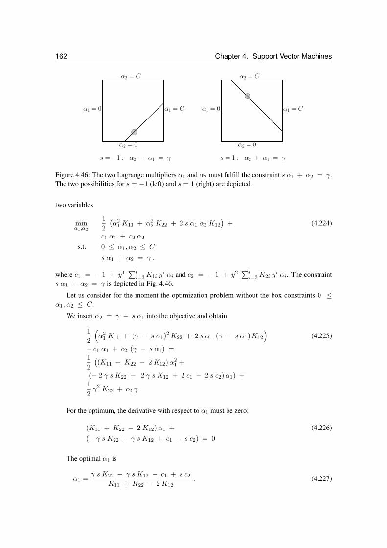
162 Chapter 4. Support Vector Machines
α1 = C
α2 = C
α2 = 0
α1 = 0 α1 = C
α2 = C
α2 = 0
α1 = 0
s = −1 : α2 − α1 = γ s = 1 : α2 + α1 = γ
Figure 4.46: The two Lagrange multipliers α1 and α2 must fulfill the constraint s α1 + α2 = γ.The two possibilities for s = −1 (left) and s = 1 (right) are depicted.
two variables
minα1,α2
12(α2
1 K11 + α22 K22 + 2 s α1 α2 K12
)+ (4.224)
c1 α1 + c2 α2
s.t. 0 ≤ α1, α2 ≤ C
s α1 + α2 = γ ,
where c1 = − 1 + y1∑l
i=3K1i yi αi and c2 = − 1 + y2
∑li=3K2i y
i αi. The constraints α1 + α2 = γ is depicted in Fig. 4.46.
Let us consider for the moment the optimization problem without the box constraints 0 ≤α1, α2 ≤ C.
We insert α2 = γ − s α1 into the objective and obtain
12
(α2
1 K11 + (γ − s α1)2K22 + 2 s α1 (γ − s α1)K12
)(4.225)
+ c1 α1 + c2 (γ − s α1) =12((K11 + K22 − 2 K12)α2
1 +
(− 2 γ s K22 + 2 γ s K12 + 2 c1 − 2 s c2)α1) +12γ2 K22 + c2 γ
For the optimum, the derivative with respect to α1 must be zero:
(K11 + K22 − 2 K12)α1 + (4.226)
(− γ s K22 + γ s K12 + c1 − s c2) = 0
The optimal α1 is
α1 =γ s K22 − γ s K12 − c1 + s c2
K11 + K22 − 2 K12. (4.227)

4.15. SVM Optimization and SMO 163
We use the discriminant function values
f(x1) =l∑
i=1
yi αi Ki1 + b (4.228)
f(x2) =l∑
i=1
yi αi Ki2 + b . (4.229)
We now can rewrite c1 and c2 as
c1 = y1 f(x1) − y1 b − 1 − K11 α1 − s K12 α2 (4.230)
c2 = y2 f(x2) − y2 b − 1 − K22 α2 − s K12 α1 (4.231)
s c2 = y1 f(x2) − y1 b − s − s K22 α2 − K12 α1 (4.232)
(4.233)
Because of
γ = α2 + s α1 (4.234)
we obtain
γ s K22 − γ s K12 = (4.235)
s K22 α2 + K22 α1 − s K12 α2 − K12 α1 .
Now we can rewrite the enumerator of eq. (4.227):
γ s K22 − γ s K12 − c1 + s c2 = (4.236)
s K22α2 + K22 α1 − s K12 α2 − K12 α1 −y1 f(x1) + y1 b + 1 + K11 α1 + s K12 α2 +y1 f(x2) − y1 b − s − s K22 α2 − K12 α1 =y1(f(x2) − f(x1)
)+
α1 (K22 + K11 − 2 K12) + 1 − s =y1((f(x2) − y2
) − (f(x1) − y1
))+
α1 (K22 + K11 − 2 K12) ,
where the last equality stems from the fact that (1 − s) = y1 (y1 − y2).
As update for α1 we obtain
αnew1 = α1 +
y1((f(x2) − y2
) − (f(x1) − y1
))K11 + K22 − 2 K12
. (4.237)
Because
s αnew1 + αnew
2 = γ = s α1 + α2 (4.238)

164 Chapter 4. Support Vector Machines
we obtain for the update of α2
αnew2 = α2 + s (α1 − αnew
1 ) . (4.239)
However we did not consider the box constraints until now.
We define as new bounds
L =
max0, α1 − α2 if s = −1max0, α1 + α2 − C otherwise
(4.240)
H =
minC,C + α1 − α2 if s = −1minC,α1 + α2 otherwise
. (4.241)
We obtain finally following update rules:
if
K11 + K22 − 2 K12 = 0 (4.242)
then
αnew1 =
H if y1
((f(x2) − y2
) − (f(x1) − y1
))> 0
L otherwise. (4.243)
else
K11 + K22 − 2 K12 > 0 (4.244)
then first compute
αtemp1 = α1 +
y1((f(x2) − y2
) − (f(x1) − y1
))K11 + K22 − 2 K12
. (4.245)
and then
αnew1 =
H if H ≤ αtemp
1
αtemp1 if L < αtemp
1 < H
L if αtemp1 ≤ L
. (4.246)
In both cases (“if” and “else” case) the update for α2 is
αnew2 = α2 + s (α1 − αnew
1 ) . (4.247)
Selection Rules.
The question arises how to chose α1 and α2.
We have to chose two αs.

4.16. Designing Kernels for Bioinformatics Applications 165
An outer loop chooses α1. This loop iterates over all patterns i which violate the KKT condi-tions. αi’s on the boundary are skipped in a first round. Afterwards also αi on the boundary aretreated.
Sometimes a whole sweep through the KKT violating data should be made to keep everythingconsistent.
The second α2 is chosen to make a large step towards the minimum. Here large steps in α areconsidered even if the objective is decreased by a small amount.
Pratt uses a heuristics where he only evaluates the numerator of the update rule. He avoidsto evaluate the kernel for checking new alphas. Therefore large differences in the relative errorsf(x1) − y1 and f(x2) − y2 are looked for.
If this heuristics for choosing α2 fails then (1) at all non-bound examples are looked then (2)all examples are looked at to make progress and finally (3) if these choices fail then a new α1 ischosen.
Other heuristics mark updated αs in order to avoid cycles where three or more αs are updatedand small progress is made. Marked αs can be updated simultaneously in a special step to avoidthe cycles.
Initially α = 0 is a good starting point and to prefer if few support vectors will be selected.
Another trick is to introduce ε from the regression setting or from the P-SVM in order to selectonly few support vectors. These support vectors can be used in another round with reduced εwhich can be viewed as annealing of support vectors.
Note that after each α update the f(xi) can be updated and sums over all α > 0 can beavoided.
Similar SMO algorithms exist for all other SVM approaches, where the regression setting withα+i and α−i can be made efficiently because only one of these α can be different from zero.
As stopping criterion the KKT conditions may be used.
4.16 Designing Kernels for Bioinformatics Applications
At the beginning of the chapter in Section 4.1, a couple of special kernels for bioinformatics havebeen mentioned.
Here we will explain some of these kernels which are relevant for bioinformatics.
Remember that every positive definite kernel is a dot product in some space as follows fromMercer’s theorem.
In general performance is optimized if the kernel is designed, i.e. an expert defines which andhow features are extracted from the original data. The mapping of the original data to the featuresis was called “feature map” and the feature map combined with dot product is a kernel.
4.16.1 String Kernel
The string kernel describes a string by all its subsequences. Subsequences do not need to becontiguous that is gaps are allowed.

166 Chapter 4. Support Vector Machines
The string kernel counts k how often the subsequence occurs and the distance t between thefirst and the last symbol. The contribution of a subsequence is
k λt , (4.248)
where 0 < λ ≤ 1 is a decay factor. Therefore, the contribution decays exponentially with thenumber of gaps.
For a subsequence all contributions of its occurrences are summed up to give the final scorefor the subsequence.
The substring “BIO” in “BIOINFORMATICS” obtains 1 · λ3 + 2 · λ7 as score, because thefollowing subsequences exist:
BIOINFORMATICS
BIOINFORMATICS
BIOINFORMATICS.
The string kernel as an upper limit n of length of the substrings it will consider. To be inde-pendent of the length of the string the feature vector is normalized to length one. A standard dotproduct or an RBF kernel can be used to perform the dot product. The string kernel is the featurevector generation together with the dot product.
4.16.2 Spectrum Kernel
The spectrum kernel is similar to the string kernel it counts occurrences of subsequences of lengthn in the string. However gaps are not allowed.
The kernel only checks whether the corresponding substring is contained in the string.
4.16.3 Mismatch Kernel
The mismatch kernel is similar to the spectrum kernel it counts occurrences of gapless subse-quences of length n with no more than m mismatches. The kernel only checks whether the corre-sponding substring is contained in the string with less or equal to m mismatches.
4.16.4 Motif Kernel
A library of motifs from PROSITE or BLOCKS or PRINTS databases is build. The occurrence ofa motif is the feature vector.
4.16.5 Pairwise Kernel
The feature vector is the vector of alignment scores to the training set. That means a new vector isaligned to all training sequences and the resulting scores give the feature vector.

4.16. Designing Kernels for Bioinformatics Applications 167
4.16.6 Local Alignment Kernel
The Smith-Waterman algorithm finds the highest scoring local alignment SW (x,y, S, g) (seeBioinformatics 1), where x and y are strings, S is a scoring Matrix (e.g. PAM or BLOSUM), andg is a gap penalty (or gap opening and extending penalty).
SW (x,y, S, g) = maxis,ie,js,je
s(x,y, S, g, is, ie, js, je) , (4.249)
where s(x,y, S, g, is, ie, js, je) is the alignment score (Needleman-Wunsch) if the subsequence(xis , . . . , xie) is aligned to (yjs , . . . , yje).
Because the Smith-Waterman score is not positive definite another kernel has to be defined.
The “local alignment kernel”
kLA(x,y, S, g, β) = (4.250)∑is=1,ie=is+1,js=1,je=js+1
exp (β s(x,y, S, g, is, ie, js, je))
is a positive definite kernel.
4.16.7 Smith-Waterman Kernel
In some application the Smith-Waterman score is used as kernel. However the theoretical basis ismissing because it is not positive definite. It may not be a dot product in some space.
But the P-SVM can naturally use the Smith-Waterman score as kernel because positive defi-niteness is not longer necessary.
4.16.8 Fisher Kernel
A class of kernels can be defined on generative models. They are very attractive because gen-erative models can deal with different sequence length, with missing or incomplete data, or withuncertainty. An advantage of generative models is that they supply a likelihood p(x;w) for newdata x which is a measure which can be interpreted statistically.
A class of kernels is defined as
kM (x,y) =∂ ln p(x;w)
∂wM−1 ∂ ln p(y;w)
∂w, (4.251)
where M = IF (w) is called the “Fisher kernel” and M = I is called the “plain kernel” whichis often used to approximate the Fisher kernel and then also called “Fisher kernel”.
The Fisher kernel was introduced for protein homology detection Jaakkola et al. [1999, 2000]where a hidden Markov model (a generative model) was trained on the positive examples. There-after a SVM with Fisher kernel was used as discriminative method which can also take into accountthe negative examples.

168 Chapter 4. Support Vector Machines
4.16.9 Profile and PSSM Kernels
The kernel working on the sequence can be generalized to kernels working on profiles or positionspecific scoring matrices (PSSMs). PSSMs are obtained by letting PSI-BLAST run against a database like NR.
Instead of the original sequence an average over very similar sequences is processed. Thesimilar sequences are found by PSI-BLAST in a large data base and then averaged by a multiplealignment. Per column of the alignment a frequency vector or a scoring vector (the PSSM) can becomputed.
Instead of alignment methods profile alignment methods must be used.
4.16.10 Kernels Based on Chemical Properties
Kernels have been suggest which take into account the chemical properties of amino acid se-quences like hydrophobicity, polarity, atomic weight, bulkiness, etc.
However these kernels where in general inferior to the kernels based on alignment or profiles.
4.16.11 Local DNA Kernel
Here DNA sequences are locally matched in a window. The window is shifted over the sequences.
This kernel is used to detect start codons where translation starts.
The kernel can be improved by shifting 3 nucleotides which accounts for frame shifts.
4.16.12 Salzberg DNA Kernel
Similar as with PSSMs also for DNA log-odd scores can be computed according to the Salzbergmethod.
4.16.13 Shifted Weighted Degree Kernel
String kernel where positions are important. “Weighted Degree Kernel” uses fixed position mea-sured with respect to a reference point. “Shifted Weighted Degree Kernel” shifts the sequencesagainst each other in order to make the positions more fuzzy.
These kernels are used to detect alternative splice sites in DNA sequences.
4.17 Kernel Principal Component Analysis
In Section 4.7 the kernel trick was mentioned. The kernel trick can be applied to every algorithmwhich is based on dot products. The kernel trick replaces the dot product by a kernel which isequivalent to mapping the vectors into a feature space and then building the dot product in thisfeature space.

4.17. Kernel Principal Component Analysis 169
The kernel trick is not always obvious because some algorithms can be formulated solely bydot products but their standard description is different.
Pre-images. Difficulties appear if the result is a vector like with clustering the cluster centers.In this case the result has to be projected back into the original space but the data points only forma sub-manifold in the feature space on which the resulting vector in general is not located on. Thisis the problem of pre-images for which different heuristics exist. However an exact solution to thisproblem is impossible because a distance measure in the feature space between the result and themanifold of data points must be defined.
We want to demonstrate the kernel trick for Principal Component Analysis (PCA) which iscalled Kernel Principal Component Analysis or kernel PCA.
PCA review. PCA computes the covariance matrixC of the data, then determinesC’s eigen-vectors w which are sorted by their eigenvalues λ. The projection xTwi of a data vector x ontothe i-th eigenvector wi is the i-th principal component of the data vector x. PCA is often usedfor dimensionality reduction or for visualization of the data. If the first k principal componentsare used to represent the data then
∑dt=k+1 λt is the expected mean squared reconstruction error
between the back-projected representation and the original data. We assume that the data wasnormalized so that
∑dt=1 λt = 1.
Kernel PCA. We assume that the data is projected into the feature space by
x 7→ Φ(x) . (4.252)
Let us for the moment assume that the data is centered in the feature space, that is
l∑i=1
Φ(xi) = 0 . (4.253)
The covariance matrix in feature space is given by
C =1l
l∑i=1
Φ(xi) ΦT (xi) . (4.254)
Note, that the Gram matrix isK =∑l
i=1 ΦT (xi)Φ(xi).
We are searching for the eigenvectors of C, i.e. for vectors fulfilling
C w = λ w . (4.255)
We are interested in solutions w which lie in the span of Φ(x1), . . . ,Φ(xl), therefore weare searching for vectors w which fulfill
∀1 ≤ n ≤ l : (λ w)TΦ(xn) = λ wTΦ(xn) = (4.256)
(C w)TΦ(xn) = wTC Φ(xn) ,
because they are unique in the span of the mapped data vectors.

170 Chapter 4. Support Vector Machines
As with SVMs the eigenvectors can be expanded with respect to the feature vectors:
w =l∑
i=1
αi Φ(xi) . (4.257)
Inserting this equation together with the definition of C in eq. (4.254) into eq. (4.256) gives
λl∑
i=1
αi ΦT (xi)Φ(xn) = (4.258)
1l
l∑i=1
αi
l∑j=1
ΦT (xi)(Φ(xj) ΦT (xj)
)Φ(xn) .
If we use the Gram matrix K with Kij = ΦT (xj)Φ(xi). This equation holds for 1 ≤ n ≤ land the vectors Φ(xn) span the whole space, therefore we obtain
l λK α = K2 α . (4.259)
To solve this equation we solve the eigenvalue problem
l λ α = K α . (4.260)
The α describes the eigenvector w which must have the length 1, resulting in
1 = wTw =(l,l)∑
ij=(1,1)
αi αj ΦT (xj)Φ(xi) = (4.261)
(l,l)∑ij=(1,1)
αi αj Kij = αTKα = l λ αTα
The vector α has to be normalized to fulfill
l λ ‖α‖2 = 1 (4.262)
‖α‖ =1√l λ
(4.263)
by
αnewi =
αi
‖α‖ √l λ (4.264)
The projection onto w can be computed as
wTΦ(x) =l∑
i=1
αi ΦT (xi)Φ(x) =l∑
i=1
αi Kij . (4.265)

4.17. Kernel Principal Component Analysis 171
Here it can be seen that the explicit representation Φ(x) is not necessary and we can setKij = k(xi,xj), i.e. to apply the kernel trick.
However the kernel trick makes the assumption of centered data more complicated becausewe want to avoid explicit representations in feature space.
Note that(Φ(xi) − 1
l
l∑t=1
Φ(xt)
)T (Φ(xj) − 1
l
l∑t=1
Φ(xt)
)= (4.266)
ΦT (xi)Φ(xj) − 1l
l∑t=1
ΦT (xt)Φ(xj) − 1l
l∑t=1
ΦT (xi)Φ(xt) +
1l2
(l,l)∑(s,t)=(1,1)
ΦT (xs)Φ(xt)
and that
1l
l∑t=1
ΦT (xt)Φ(xi) =[
1lK 1
]i
(4.267)
1l
l∑t=1
ΦT (xi)Φ(xt) =[
1l1TK
]i
1l2
(l,l)∑(s,t)=(1,1)
ΦT (xs)Φ(xt) =1l2
1TK 1 .
Therefore the following equations produces a centered kernel matrix:
K − 1lK 1 1T − 1
l1 1TK +
1l2(1TK 1
)1 1T . (4.268)
A new data point x can be centered by first computing
k(x, .) =(k(x,x1), . . . , k(x,xl)
)T(4.269)
and then
k(x, .) − 1lK 1 − 1
l1Tk(x, .) 1 +
1l2(1TK 1
)1 . (4.270)
Kernel PCA works as follows:
center the Gram matrix according to eq. (4.268)
compute eigenvectors and eigenvalues of the Gram matrixK

172 Chapter 4. Support Vector Machines
Figure 4.47: Kernel PCA example. Top left: original data. From top middle to upper right the8 first principal components are depicted. The first two separate the clusters, the next 3 (mid-dle panel) split the clusters, and the next 3 (bottom panel) split them orthogonal to the previous3 components. An RBF-kernel with k(xi,xj) = exp
(− 10 ‖xi − xj‖2 ) was used. From[Schölkopf et al., 1998]
normalize eigenvectors α according to eq. (4.264)
project a new vector x onto eigenvectors by first centering it using eq. (4.270) and thenaccording to eq. (4.265).
Kernel PCA toy examples are shown in Figures 4.47 and 4.48.
4.18 Kernel Discriminant Analysis
Here we will apply the kernel trick to another well known method: “Linear Discriminant Analysis”(LDA) or “Fisher Discriminant Analysis” (FDA).
Let us assume we have a binary problem as with the SVM approach. The Fisher discriminantalgorithm maximizes the Rayleigh coefficient J with respect to w:
J(w) =wTM w
wTN w, (4.271)

4.18. Kernel Discriminant Analysis 173
Figure 4.48: Another kernel PCA example. Each column corresponds to one method based onPCA. Each column gives the three largest eigenvalues with the according eigenvectors depicted ascontour lines. In the first column linear PCA, and in the second, third and last column polynomialkernel with degree 2,3, and 4, respectively, is shown. From [Schölkopf and Smola, 2002]

174 Chapter 4. Support Vector Machines
where
M = (m− − m+) (m− − m+)T (4.272)
is the between class variance and
N =l∑
i=1;yi=1
(xi − m+
) (xi − m+
)T + (4.273)
l∑i=1;yi=−1
(xi − m−
) (xi − m−
)Tis the within class variance.
The Fisher’s discriminant attempts at minimizing the variance within one class whilst separat-ing the class centers a good as possible.
Let l+ be the number of class 1 examples and l− the number of class -1 examples
Here we used the mean values
m+ =1l+
l∑i=1;yi=1
xi (4.274)
m− =1l−
l∑i=1;yi=−1
xi (4.275)
Note that
wTM w =(wTm− − wTm+
) (mT−w − mT
+w)
(4.276)
and
wTN w = (4.277)l∑
i=1;yi=1
(wTxi − wTm+
) ((xi)Tw − mT
+w)
+
l∑i=1;yi=−1
(wTxi − wTm−
) ((xi)Tw − mT
−w)
Now we proceed like with the kernel PCA and set
w =l∑
i=1
αi Φ(xi) . (4.278)
LetK be again the Gram matrix with Kij = k(xi,xj) = ΦT (xi) Φ(xj)
4.18. Kernel Discriminant Analysis 175
We use expansion of w according to eq. (4.278) and obtain
wTm− =1l−
l∑j=1;yj=−1
wTΦ(xj) = (4.279)
1l−
l∑j=1;yj=−1
l∑i=1
αi ΦT (xi) Φ(xj) =
1l−
l∑j=1;yj=−1
l∑i=1
αi k(xi,xj) .
We use again
k(x, .) =(k(x,x1), . . . , k(x,xl)
)T(4.280)
and define
µ− =1l−
l∑j=1;yj=−1
k(xj , .) =1l−K 1− (4.281)
to obtain
wTm− = αTµ− . (4.282)
Here we used 1− the l-dimensional vector which has ones at positions of class -1 examples and 0otherwise.
Analog using
µ+ =1l+
l∑j=1;yj=1
k(xj , .) =1l+K 1+ (4.283)
we obtain
wTm+ = αTµ+ . (4.284)
We used 1+ the l-dimensional vector which has ones at positions of class 1 examples and 0 other-wise.
wTM w =(αTµ− − αTµ+
) (µT−α − µT+α
)= (4.285)
αT (µ− − µ+) (µ− − µ+)T α =(αT (µ− − µ+)
)2=
αTMk α ,

176 Chapter 4. Support Vector Machines
where
Mk = (µ− − µ+) (µ− − µ+)T . (4.286)
The expansion of w according to eq. (4.278) gives
wTN w =l∑
j=1;yj=1
(l∑
i=1
αi ΦT (xi)Φ(xj) − wTm+
)(4.287)
(l∑
i=1
αi ΦT (xj)Φ(xi) − mT+w
)+
l∑j=1;yj=−1
(l∑
i=1
αi ΦT (xi)Φ(xj) − wTm−
)(
l∑i=1
αi ΦT (xj)Φ(xi) − mT−w
)=
(l,l)∑i,n=(1,1)
αi αn
l∑j=1;yj=1
ΦT (xi)Φ(xj)ΦT (xj)Φ(xi) −
l+
l∑i=1
αi µ+ αTµ+ −
l+
l∑i=1
αi µ+ µT+α + l+ µ
T+α µ
T+α +
(l,l)∑i,n=(1,1)
αi αn
l∑j=1;yj=−1
ΦT (xi)Φ(xj)ΦT (xj)Φ(xi) −
l−l∑
i=1
αi µ− αTµ− −
l−l∑
i=1
αi µ− µT−α + l− µT−α µT−α =
(l,l)∑i,n=(1,1)
αi αn
l∑j=1
KijKji − l+ αTµ+ µ
T+α −
l− αTµ− µT−α =αT(K KT − l+ µ+ µ
T+ − l− µ− µT−
)α .
If we define
Nk = K KT − l+ µ+ µT+ − l− µ− µT− (4.288)

4.18. Kernel Discriminant Analysis 177
Figure 4.49: Kernel discriminant analysis (KDA) example. Left: KDA contour lines. Middleand Right: first and second component of kernel PCA. With KDA the contour lines are useful toseparate the data. From [Mika et al., 1999].
then
wTN w = αTNk α . (4.289)
We obtain for the kernel version of Fisher’s discriminant the following Rayleigh coefficient tomaximize:
J(α) =αTMk α
αTNk α. (4.290)
The projection of a new vector onto the discriminant direction w is
wT Φ(x) =l∑
i=1
αi ΦT (xi)Φ(x) =l∑
i=1
αi k(xi,x) . (4.291)
The Rayleigh coefficient eq. (4.290) can be maximized by the generalized eigenvalue problem
Mk α = λNk α (4.292)
and selecting the eigenvector with maximal eigenvalue λ.
However until now the regularization, i.e. the capacity control was not considered. It is im-portant for kernel methods because the l dimensional covariance matrixNk is estimated by l datapoints.
One approach for regularization is to replaceNk by
Nk + εI . (4.293)
Fig. 4.49 shows a toy example for kernel discriminant analysis (KDA) compared with kernelPCA.

178 Chapter 4. Support Vector Machines
However the idea of kernel Fisher discriminant analysis can be written in a more convenientform.
First assume that we affine transform the data in a way that
wTm+ + b = 1 (4.294)
and
wTm− + b = −1 . (4.295)
That means the between class variance is fixed.
Now we have only to minimize the variance of the data points around their class mean (-1 or+1). If we set
wTxi + b = yi + ξi (4.296)
then ξi gives the deviation of the projected xi from its class label.
In order that 1 is the mean projection value of class 1 data points and −1 the mean projectionvalue of class -1 data points, we must ensure that
1+ ξ = 0 and (4.297)
1− ξ = 0 . (4.298)
The class 1 variance plus the class 2 variance is given by
ξT ξ = ‖ξ‖2 . (4.299)
This variance must be minimized.
Using as regularization term either ‖α‖2 or αTK α we obtain the following quadratic pro-grams:
minα,ξ,b
‖ξ‖2 + C ‖α‖2 (4.300)
s.t. K α + b1 = y + ξ
1+ ξ = 0 and
1− ξ = 0
or
minα,ξ,b
‖ξ‖2 + CαTK α (4.301)
s.t. K α + b1 = y + ξ
1+ ξ = 0 and
1− ξ = 0 .
Note, that this formulation is very similar to the least square SVM in Subsection 4.13. K α =XTw if w = X α andK = XTX . Here the errors per class are forced to have mean zero.

4.19. Software 179
4.19 Software
Online applets for SVM demos are available under
http://www.eee.metu.edu.tr/~alatan/Courses/Demo/AppletSVM.html and
http://www.csie.ntu.edu.tw/~cjlin/libsvm/.
From these sources some screen shots are made in above examples.
Software can be found under
http://www.kernel-machines.org,
http://www.support-vector-machines.org/SVM_stat.html, and
http://kernelsvm.tripod.com.
Software packages which we recommend are
P-SVM: http://www.bioinf.jku.at/software/psvm/.
• For UNIX and WINDOWS.
• Matlab front end.
• Cross-validation included.
• Feature selection included.
• Non-positive definite kernels possible.
• Significance tests.
libSVM: http://www.csie.ntu.edu.tw/~cjlin/libsvm/.
• For UNIX and WINDOWS.
• Sparse matrices.
• Phyton scripts for hyperparameter selection. Front ends for Python, R (also Splus),MATLAB, Perl, Ruby, Weka, CLISP and LabVIEW.
• C# .NET code is available.
• Cross-validation included.
• Multi-class.
SVM-light: http://svmlight.joachims.org/.
• For UNIX and WINDOWS.
SVMTorch: http://www.idiap.ch/~bengio/projects/SVMTorch.html orhttp://www.torch.ch/.
• UNIX.
• Sparse matrices.
• Multi-class.

180 Chapter 4. Support Vector Machines

Chapter 5
Error Minimization andModel Selection
We focus on a model class of parameterized models with parameter vector w. Goal is to find orto select the optimal model. The optimal model is the one which optimizes the objective function.To find the optimal model, we have to search in the parameter space.
The objective function is defined by the problem to solve. In general the objective functionincludes the empirical error and a term which penalizes complexity. The goal is to find the modelfrom the model class which optimizes the objective function.
5.1 Search Methods and Evolutionary Approaches
In principle any search algorithm can be used. The simplest was is random search, where randomlya parameter vector is selected and then evaluated – the so far best solution is kept.
Another method would be exhaustive search, where the parameter space is searched system-atically.
These two methods will find the optimal solution for a finite set of possible parameters. Theydo not use any dependency between objective function and parameter space. For example, if theobjective function should be minimized and is 1 for every parameter w except for one parameterwopt which gives 0. That is a singular solution.
In general there are dependencies between objective function and parameters. These depen-dencies should be utilized to find the model which optimizes the objective function.
The first dependency is that good solutions are near good solutions in parameter space even ifthe objective is not continuous and not differentiable. In this case a stochastic gradient can be usedto locally optimize the objective function. In the context of genetic algorithms a stochastic gradi-ent corresponds to mutations which are small. With “small” we mean that every component, e.g.“gene” is mutated only slightly or only one component is mutated at all. In general a stochasticgradient tests solutions which are similar the current best solution or current best solutions. Fi-nally an update of the current best solution is made sometimes by combining different parameterchanges which improved the current best solution.
Another dependency is that good solutions share properties of their parameter vector whichare independent of other components of the parameter vector. For example if certain dependencies
181

182 Chapter 5. Error Minimization and Model Selection
between specific parameters guarantee good solutions and these specific parameters do not influ-ence other parameters. In this case genetic algorithms can utilize these dependencies through the“crossover mutations” where parts of different parameter vectors are combined. Important is thatcomponents are independent of other components, i.e. the solutions have different building blockswhich can improve the objective independently of other building blocks.
Besides the genetic algorithms there are other evolutionary strategies to optimize models.These strategies include genetic programming, swarm algorithms, ant algorithms, self-modifyingpolicies, Optimal Ordered Problem Solver, etc. Sometimes the model class is predefined by thesearch algorithm or the model class is not parameterized. The latter even modify their own searchstrategy.
All these methods have to deal with local optima of the objective function. To reduce theproblem of optima, genetic algorithms search in general at different locations in the parameterspace simultaneously. Also other approaches search in parallel at different locations in parameterspace.
To overcome the problem of local optima simulated annealing (SA) has been suggested. SAcan be shown to find the global solution with probability one if the annealing process is slowenough. SA probabilistic jumps from the current state into another state where the probabilityis given by the objective function. The objective function is transformed to represent an energyfunction, so that SA jumps into energetically favorable states. The energy function follows theMaxwell-Boltzmann distribution and the sampling is similar to the Metropolis-Hastings algorithm.A global parameter, the temperature, determines which jumps are possible. At the beginning largejumps even into energetically worse regions are possible due to high temperature whereas with lowtemperature only small jumps are possible and energetically worse regions are avoided. Thereforethe parameter space is at the beginning scanned for favorable regions where later is searched inmore detail.
Advantages of these methods are that they
can deal with discrete problems and non-differentiable objective functions and
are very easy to implement.
Disadvantages of these methods are that they
are computationally expensive for large parameter spaces and
depend on the representation of the model.
To see the computational load of stochastic gradient or genetic algorithms assume that theparameter vector has W components. If we only check whether these components should beincreased or decreased, we have 2W decisions to make. When the amount of change also mattersthen this number of candidates will be soon infeasible to check only to make one improvementstep.
The dependency between the parameter space and the objective function which will be of in-terest in the following is that the objective function is differentiable with respect to the parameters.
Therefore we can make use of gradient information in the search of the (local) minimum.

5.2. Gradient Descent 183
tangent on (R(w), w)
R(w)
w
− g
− g
tangent on (R(w), w)
Figure 5.1: The negative gradient − g gives the direction of the steepest decent depicted by thetangent on (R(w),w), the error surface.
Problems like that were already treated in Section 4.15 in Subsection 4.15.1. However wefocused on convex optimization. There only one minimum exists. Further we treated linear andquadratic objectives. The idea of Lagrange multipliers carries over to constraint optimization ingeneral: assume that the problem is locally convex.
5.2 Gradient Descent
Assume that the objective function R(g(.;w)) is a differentiable function with respect to the pa-rameter vectorw. The function g is the model. For simplicity, we will writeR(w) = R(g(.;w)).
The gradient is
∂R(w)∂w
= ∇wR(w) =(∂R(w)∂w1
, . . . ,∂R(w)∂wW
)T, (5.1)
for a W -dimensional parameter vector w.
For the gradient of R(w) we use the vector
g = ∇wR(w) . (5.2)
The negative gradient is the direction of the steepest descent of the objective. The negativegradient is depicted in Fig. 5.1 or a one-dimensional error surface and in Fig. 5.2 for a two-dimensional error surface.
Because the gradient is valid only locally (for nonlinear objectives) we only go a small stepin the negative gradient direction if we want to minimize the objective function. The step-size iscontrolled by 0 < η, the learning rate.

184 Chapter 5. Error Minimization and Model Selection
−g
−g
−g
−g
Figure 5.2: The negative gradient − g attached at different positions on an two-dimensional errorsurface (R(w),w). Again the negative gradient gives the direction of the steepest descent.
The gradient descent update is
∆w = − η ∇wR(w) (5.3)
wnew = wold + ∆w . (5.4)
Momentum Term. Sometimes gradient descent oscillates or slows down because the errorsurface (the objective function) has a flat plateau. To avoid oscillation and to speed up gradientdescent a momentum term can be used. The oscillation of the gradient is depicted in Fig. 5.3 andthe reduction of oscillation through the momentum term in Fig. 5.4.
Another effect of the momentum term is that in flat regions the gradients pointing in the samedirections are accumulated and the learning rate is implicitly increased. The problem of flat regionsis depicted in Fig. 5.5 and the speed up of the convergence in flat regions in Fig. 5.6.
The gradient descent update with momentum term is
∆neww = − η ∇wR(w) (5.5)
wnew = wold + ∆neww + µ ∆old (5.6)
∆old = ∆new , (5.7)
where 0 ≤ µ ≤ 1 is the momentum parameter or momentum factor.
5.3 Step-size Optimization
Instead of choosing a fixed step-size the step-size should be adjusted to the curvature of the errorsurface. For a flat curve the step-size could be large whereas for high curvature and steep minimathe step-size should be small. In Fig. 5.7 the

5.3. Step-size Optimization 185
−g
w2
w1
Figure 5.3: The negative gradient − g oscillates as it converges to the minimum.
−g
w2
w1
Figure 5.4: Using the momentum term the oscillation of the negative gradient − g is reducedbecause consecutive gradients which point in opposite directions are superimposed. The minimumfound faster.
−g
w2
w1
Figure 5.5: The negative gradient − g let the weight vector converge very slowly to the minimumif the region around the minimum is flat.
−g
w2
w1
Figure 5.6: The negative gradient − g is accumulates through the momentum term because con-secutive gradients point into the same directions. The minimum found faster.
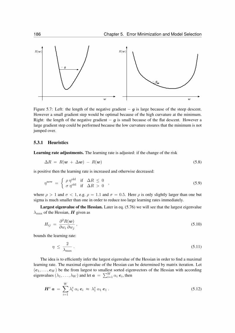
186 Chapter 5. Error Minimization and Model Selection
R(w)
w w
− g
− g
R(w)
Figure 5.7: Left: the length of the negative gradient − g is large because of the steep descent.However a small gradient step would be optimal because of the high curvature at the minimum.Right: the length of the negative gradient − g is small because of the flat descent. However alarge gradient step could be performed because the low curvature ensures that the minimum is notjumped over.
5.3.1 Heuristics
Learning rate adjustments. The learning rate is adjusted: if the change of the risk
∆R = R(w + ∆w) − R(w) (5.8)
is positive then the learning rate is increased and otherwise decreased:
ηnew =ρ ηold if ∆R ≤ 0σ ηold if ∆R > 0
, (5.9)
where ρ > 1 and σ < 1, e.g. ρ = 1.1 and σ = 0.5. Here ρ is only slightly larger than one butsigma is much smaller than one in order to reduce too large learning rates immediately.
Largest eigenvalue of the Hessian. Later in eq. (5.76) we will see that the largest eigenvalueλmax of the Hessian,H given as
Hij =∂2R(w)∂wi ∂wj
, (5.10)
bounds the learning rate:
η ≤ 2λmax
. (5.11)
The idea is to efficiently infer the largest eigenvalue of the Hessian in order to find a maximallearning rate. The maximal eigenvalue of the Hessian can be determined by matrix iteration. Let(e1, . . . , eW ) be the from largest to smallest sorted eigenvectors of the Hessian with accordingeigenvalues (λ1, . . . , λW ) and let a =
∑Wi=1 αi ei, then
Hs a =W∑i=1
λsi αi ei ≈ λs1 α1 e1 . (5.12)

5.3. Step-size Optimization 187
Normalizing Hs a and multiplication with H gives both a hint how well e1 is approximated andhow large λ1 may be.
The method depends how time intensive it is to obtain the Hessian or the product of the Hessianwith a vector. How the Hessian is computed depends on the model. For quadratic problems theHessian is directly given and for neural networks there exist different methods to approximate theHessian or to compute the product of the Hessian with a vector. See Section 6.4.4 for more details.
Individual learning rate for each parameter.
We have for parameter wi
∆wi = − ηi gi , (5.13)
where gi is the i-th component of the gradient g: gi =[∂R(w)∂w
]i. If the parameters would be
independent from each other, then individual learning rates are justified. However for dependentparameter, as long as all ηi > 0 the error decreases.
The delta-delta rule adjusts the local learning parameter according to
∆ηi = γ gnewi gold
i . (5.14)
The delta-delta rule determines whether the local gradient information changes. If it changesthen the learning rate is decreased otherwise it is increased. In a flat plateau the learning rate isincreased and in steep regions the learning rate is decreased.
This rule was improved to the delta-bar-delta rule:
∆ηi =κ if gold
i gnewi > 0
− φ gnewi if gold
i gnewi ≤ 0
, (5.15)
where
gnewi = (1 − θ) gnew
i + θ goldi . (5.16)
gi is an exponentially weighted average of the values of gi. That means instead of the old gradientinformation an average is used to determine whether the local gradient directions changes.
Big disadvantage of the delta-bar-delta rule that it has many hyper-parameters: θ, κ, φ and µif a momentum term is included as well.
Quickprop. This method was developed in the context of neural networks, therefore the name“quickprop” which reminds on the name “back-propagation” the most popular method for com-puting the gradient in neural networks.
Here again the parameters are treated individually. The quickprop learning rule is
∆newwi =gi
goldi − gnew
i
∆oldwi . (5.17)

188 Chapter 5. Error Minimization and Model Selection
R(w)
w
Figure 5.8: The error surface (the solid curve) is locally approximated by a quadratic function (thedashed curve).
Let us assume that R(w) is a function of one variable R(wi) then the Taylor expansion is
R(wi + ∆wi) = R(wi) +∂R(w)∂wi
∆wi + (5.18)
12∂2R(w)(∂wi)2
(∆wi)2 + O((∆wi)3
)=
R(wi) + gi ∆wi +12g′i (∆wi)2 + O
((∆wi)3
).
That is a quadratic approximation of the function. See Fig. 5.8 for the quadratic approximation ofthe error function R(w).
To minimize R(wi + ∆wi) − R(wi) with respect to ∆wi we set the derivative of the righthand side to zero and obtain
∆wi = − gig′i. (5.19)
Now approximate g′i = g′i(wi) by g′i(woldi ) and use a difference quotient:
g′i =gnewi − gold
i
∆oldwi, (5.20)
where goldi = gi(wi − ∆oldwi). We now insert this approximation into eq. (5.19) which results
in the quickprop update rule.
5.3.2 Line Search
Let us assume we found the update direction d either as the negative gradient or by also takinginto account the curvature by the Hessian or its approximation.

5.3. Step-size Optimization 189
The update rule is
∆w = η d . (5.21)
We now want to find the value of η which minimizes
R(w + η d) . (5.22)
For quadratic functions and d = − g and very close to the minimum w∗, η is given later ineq. (5.77) as
η =gT g
gT H(w∗) g. (5.23)
However this is only valid near the minimum. Further we do not knowH(w∗).
Finding the best update step could be viewed as a separate task. If we assume that at theminimum the function R(w) is convex then we can apply line search.
Line search fits first a parable though three points and determines its minimum. The point withlargest value of R is discharged. The line search algorithm is given in Alg. 5.1.
Algorithm 5.1 Line Search
BEGIN initialization a0, b0, c0;R(a0) > R(c0);R(b0) > R(c0), Stop=false, i = 0END initializationBEGIN line search
while STOP=false dofit quadratic function through ai, bi, cidetermine minimum di of quadratic functionif stop criterion fulfilled, e.g. |ai − bi| < ε or |R(b0)−R(c0)| < ε then
Stop=trueelseci+1 = dibi+1 = ci
ai+1 =ai if R(ai) ≤ R(bi)bi if R(ai) > R(bi)
end ifi = i+ 1
end whileEND line search
Fig. 5.9 shows the line search procedure. At each step the length of the interval [a, b] or [b, a]is decreased.
Line search starts with R(w), R(w + η0d) and R(w + ηmax d) , where a0, b0, c0 ∈eta0, 0, etamax. If a large range of η values are possible, then the search can be on a logarithmicscale as preprocessing.
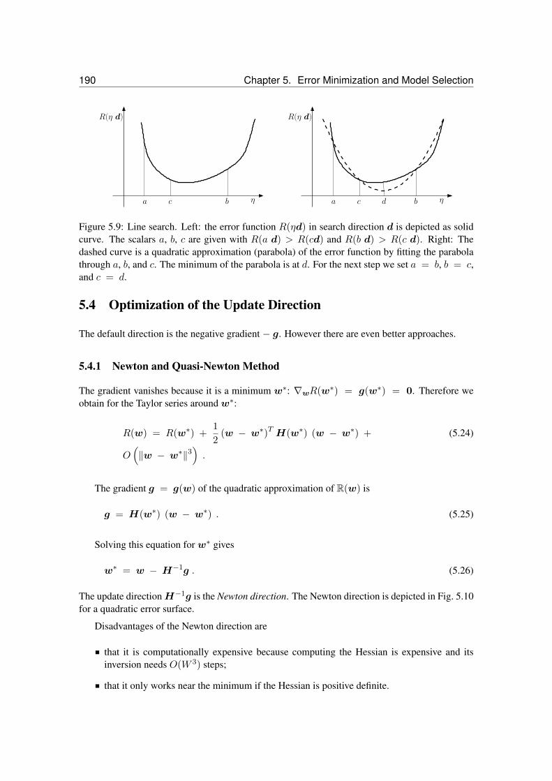
190 Chapter 5. Error Minimization and Model Selection
ηbca
R(η d)
η bdca
R(η d)
Figure 5.9: Line search. Left: the error function R(ηd) in search direction d is depicted as solidcurve. The scalars a, b, c are given with R(a d) > R(cd) and R(b d) > R(c d). Right: Thedashed curve is a quadratic approximation (parabola) of the error function by fitting the parabolathrough a, b, and c. The minimum of the parabola is at d. For the next step we set a = b, b = c,and c = d.
5.4 Optimization of the Update Direction
The default direction is the negative gradient − g. However there are even better approaches.
5.4.1 Newton and Quasi-Newton Method
The gradient vanishes because it is a minimum w∗: ∇wR(w∗) = g(w∗) = 0. Therefore weobtain for the Taylor series around w∗:
R(w) = R(w∗) +12
(w − w∗)T H(w∗) (w − w∗) + (5.24)
O(‖w − w∗‖3
).
The gradient g = g(w) of the quadratic approximation of R(w) is
g = H(w∗) (w − w∗) . (5.25)
Solving this equation for w∗ gives
w∗ = w − H−1g . (5.26)
The update directionH−1g is the Newton direction. The Newton direction is depicted in Fig. 5.10for a quadratic error surface.
Disadvantages of the Newton direction are
that it is computationally expensive because computing the Hessian is expensive and itsinversion needs O(W 3) steps;
that it only works near the minimum if the Hessian is positive definite.

5.4. Optimization of the Update Direction 191
− H−1 g
w2
w1
−g
Figure 5.10: The Newton direction − H−1 g for a quadratic error surface in contrast to thegradient direction − g. The Newton direction points directly to the minimum and one Newtonupdate step would find the minimum.
A remedy for the later disadvantage is the model trust region approach, where the model isonly trusted up to a certain value. A positive definite matrix is added to the Hessian:
H + λI . (5.27)
The update step is a compromise between gradient direction (large λ) and Newton direction(lambda = 0).
To address the problem of the expensive inversion of the Hessian, it can be approximated by adiagonal matrix. The diagonal matrix is simple to invert.
Quasi-Newton Method.From the Newton equation eq. (5.26) two weight vectors wold and wnew are related by
wnew − wold = −H−1(gnew − gold
). (5.28)
This is the quasi-Newton condition.
The best known method is the Broyden-Fletcher-Goldfarb-Shanno (BFGS) method. TheBFGS update is
wnew = wold + η Gold gold , (5.29)
where η is found by line search.
The functionG is an approximation of the inverse Hessian and is computed as follows:
Gnew = Gold +p pT
pT v− (5.30)(
Gold v)vTGold
vTGold v+(vTGold v
)u uT ,
where
p = wnew − wold (5.31)
v = gnew − gold (5.32)
u =p
pTv− Goldv
vTGold v. (5.33)

192 Chapter 5. Error Minimization and Model Selection
w2
w1
−g
d
Figure 5.11: Conjugate gradient. After line search in search direction d the new gradient is or-thogonal to the line search direction.
Initialization ofG can be done by I , the identity matrix (only a gradient step as first step).
5.4.2 Conjugate Gradient
Note that for the line search algorithm we optimized η so that
R(w + η d) (5.34)
is minimized.
The minimum condition is
∂
∂ηR(w + η d) = 0 , (5.35)
which gives
(gnew)T dold = 0 . (5.36)
The gradient of the new minimum gnew is orthogonal to the previous search direction dold. Thisfact is depicted in Fig. 5.11.
However still oscillations are possible. The oscillations appear especially in higher dimen-sions, where oscillations like in Fig. 5.3 can be present in different two-dimensional subspaceswhich alternate. Desirable to avoid oscillations would be that a new search directions are orthogo-nal to all previous search directions where orthogonal is defined via the Hessian. The later meansthat in the parameter space not all directions are equal important. In the following we constructsuch search directions.
The oscillations can be avoided if we enforce not only
g(wnew)T dold = 0 (5.37)
but also the same condition for the new gradient
g(wnew + ηdnew)T dold = 0 . (5.38)

5.4. Optimization of the Update Direction 193
d1
d3
d4
d2
d3
d4d2
d1
Figure 5.12: Conjugate gradient. Left: dT1 d2 = 0 and dT3 d4 = 0. Right: dT1 H d2 = 0and dT3 H d4 = 0. Conjugate directions can be viewed as orthogonal directions which weretransformed by a change of the coordinate system: d = H−1/2d.
Taylor expansion of g(wnew + ηdnew) with respect to η around 0 gives
g(wnew + ηdnew)T = g(wnew) + ηH(wnew)dnew + O(η2) . (5.39)
We insert that into eq. (5.38) and apply eq. (5.37) and divide through η and obtain
(dnew)T H(wnew) dold = 0 . (5.40)
Directions which satisfy eq. (5.40) are said to be conjugate. See Fig. 5.12 for conjugate direc-tions.
Let us assume a quadratic problem
R(w) =12wTHw + cTw + k (5.41)
with
g(w) = Hw + c (5.42)
and
0 = Hw∗ + c . (5.43)
We want to have W conjugate directions, i.e.
∀i 6=j : dTjH di = 0 , (5.44)
which are linearly independent, therefore we can set
w∗ − w1 =W∑i=1
ηi di (5.45)
(5.46)

194 Chapter 5. Error Minimization and Model Selection
and
wj − w1 =j−1∑i=1
ηi di . (5.47)
In the last but one equation w∗ = −H−1 c is multiplied by dTjH and we obtain
− dTj (c + Hw1) =W∑i=1
ηi dTjH di = ηj d
TjH dj . (5.48)
From eq. (5.47) we obtain
dTjH wj = dTjH w1 . (5.49)
Using gj = c + Hwj , ηj can be determined as
ηj = − dTj gj
dTjH dj. (5.50)
Because of
wj+1 = wj + ηj dj . (5.51)
we have determined the learning rate ηj .
Now we have find the search directions dj . We set
dj+1 = − gj+1 + βj dj . (5.52)
Multiplying by dTjH gives
βj =gTj+1H dj
dTjH dj. (5.53)
Because of
gj+1 − gj = H (wj+1 − wj) = ηj H dj (5.54)
we can rewrite eq. (5.53) as
Hestenes− Stiefel : (5.55)
βj =gTj+1 (gj+1 − gj)
dTj (gj+1 − gj). (5.56)

5.4. Optimization of the Update Direction 195
Multiplying eq. (5.52) by gTj+1 and using the conditions dTk gj = 0 for k < j gives
dTj gj = − gTj gj . (5.57)
The equation for βj can be rewritten as
Polak−Ribiere : (5.58)
βj =gTj+1 (gj+1 − gj)
gTj gj. (5.59)
Similar to previous reformulation this expression can be simplified to
Fletcher−Reeves : (5.60)
βj =gTj+1gj+1
gTj gj. (5.61)
Even if the equations eq. (5.55), eq. (5.58), and eq. (5.60) are mathematically equivalent, thereare numerical differences. The Polak-Ribiere equation eq. (5.58) has an edge over the other updaterules.
The computation of the values ηj need the Hessian, therefore the ηj are in most implementa-tions found by line search.
Algorithm 5.2 Conjugate Gradient (Polak-Ribiere)
BEGIN initialization g0 = ∇wR(w0), i = 0,d0 = −g0, Stop=falseEND initializationBEGIN Conjugate Gradient
while STOP=false dodetermine ηi by line searchwj+1 = wj + ηj djgi+1 = ∇wR(wi)
βj =gTj+1(gj+1 − gj)
gTj gj
dj+1 = − gj+1 + βj djif stop criterion fulfilled, e.g. ‖gi+1‖| < ε or |R(wj+1)−R(wj)| < ε then
STOP=trueend ifi = i+ 1
end whileEND Conjugate Gradient
The disadvantage of conjugate gradient compared to the quasi-Newton methods is
the line search must be done precisely in order to obtain the conjugate and orthogonal gra-dients
The advantage of conjugate gradient compared to the quasi-Newton methods is
that the storage is O(W ) compared to O(W 2) for quasi-Newton

196 Chapter 5. Error Minimization and Model Selection
5.5 Levenberg-Marquardt Algorithm
This algorithm is designed for quadratic loss, i.e. for the mean squared error
R(w) =l∑
i=1
(ei(w)
)2. (5.62)
We combine the errors ei into a vector e. The Jacobian of this vector is Z defined as
Zij =∂ei
∂wj. (5.63)
The linear approximation of the error vector gives
e(wnew) = e(wold) + Z(wnew − wold
). (5.64)
The Hessian of the loss function R(w) is
Hjk =∂2R
∂wj ∂wk=
l∑i=1
(∂ei
∂wj
∂ei
∂wk+ ei
∂2ei
∂wj ∂wk
). (5.65)
If we assume small ei (if we are close to the targets) or if we assume that the term ei ∂2ei
∂wj ∂wkaverages out, then we can approximate the Hessian by
H = ZTZ . (5.66)
Note that this “outer product approximation” is only valid for quadratic loss functions.
We now can formulate a unconstraint minimization problem where
12
∥∥∥e(wold) + Z(wnew − wold
)∥∥∥2+ λ
∥∥∥wnew − wold∥∥∥2
(5.67)
has to be minimized. The first term accounts for minimizing the error and the second term forminimizing the step size.
The solution is the Levenberg-Marquardt update rule
wnew = wold − (ZTZ + λ I
)−1ZT e(wold) . (5.68)
Small λ gives the Newton formula while large λ gives gradient descent.
The Levenberg-Marquardt algorithm is a model trust region approach.

5.6. Predictor Corrector Methods for R(w) = 0 197
5.6 Predictor Corrector Methods for R(w) = 0
The problem is to solve R(w) = 0. That problem is different from minimization problems.
The idea is to make a simple update (predictor step) by neglecting higher order terms. In asecond step (corrector step) the value is corrected by involving the higher order terms. Here thehigher order terms are evaluated with the solution obtained by the predictor step.
The Taylor series of R(wnew) is
R(wnew) = R(wold) + S(wold,∆w) + TS(wold,∆w) . (5.69)
Here S(wold,0) = 0 and T (wold,0) = 0.
In the predictor step solve
R(wold) + S(wold,∆w) = 0 (5.70)
with respect to ∆w which gives ∆predw. In the corrector step solve
R(wold) + S(wold,∆w) + TS(wold,∆predw) = 0 , (5.71)
which gives the final update ∆w.
The predictor-corrector update can be formulated as an iterative algorithm.
5.7 Convergence Properties
Gradient Descent. We make a Taylor series expansion of the gradient function g locally at theminimum w∗. The gradient vanishes because it is a minimum ∇wR(w∗) = g(w∗) = 0,therefore we obtain
R(w) = R(w∗) +12
(w − w∗)T H(w∗) (w − w∗) + (5.72)
O(‖w − w∗‖3
).
The improvement of the risk is
R (w − η g) − R(w∗) = (5.73)12
(w − η g − w∗)T H(w∗) (w − η g − w∗) =
12η2 gT H(w∗) g − η gT g + c ,
where c is independent of η.
First we note that
12η2 gT H(w∗) g − η gT g ≤ 0 , (5.74)

198 Chapter 5. Error Minimization and Model Selection
to ensure improvement for arbitrary c. That is equivalent to
η ≤ 2 gT ggT H(w∗) g
, (5.75)
which gives the bound (the g which gives the smallest value)
η ≤ 2λmax
. (5.76)
The optimal update is obtained if we minimize the left hand side of eq. (5.74) with respect toη. Setting the derivative with respect to η to zero an solving for η gives
η =gT g
gT H(w∗) g. (5.77)
The update is
wnew = wold − gT g
gT H(w∗) gg . (5.78)
The improvement is
R(wold
)− R (wnew) = (5.79)(
wold − w∗)H(w∗)
gT g
gT H(w∗) gg −
12
(gT g
gT H(w∗) g
)2
gT H(w∗) g =
12
(gT g
)2gT H(w∗) g
= R(wold
)( (gT g
)2(gT H(w∗) g) (gT H−1(w∗) g)
).
The Kantorovich inequality states that(gT g
)2(gT H g) (gT H−1 g)
≥ 4 λmin λmax
(λmin + λmax)2 ≥1
cond(H), (5.80)
where and λmax and λmin are the maximal and minimal eigenvalues of the Hessian, respectively,and cond(H) is the condition of a matrix
cond(H) =λmax
λmin. (5.81)
The improvement depends strongly on the condition of the matrixH(w∗).
Newton Method.

5.7. Convergence Properties 199
The Newton method has the update rule:
wnew = wold − ∇wR(wold)H−1(wold) . (5.82)
With previous definitions and Taylor expansion of R around w∗ we have g(w∗) = 0.
The Taylor expansion of the i-th component of g around wold is
0 = gi(w∗) = gi(wold) + ∇wgi(wold)(w∗ − wold
)+ (5.83)
ξTHi(wold) ξ ,
where Hi is the Hessian of gi and ξ is a vector ξi = λ(w∗ − wold
)with 0 ≤ λ ≤ 1, thus
‖ξi‖2 ≤∥∥w∗ − wold
∥∥.
We obtain
gi(wold) = gi(wold) − gi(w∗) = gi(wold) − (5.84)(gi(wold) +
(w∗ − wold
)T ∇wgi(wold) +
12ξTi Hi(wold) ξi
).
Combining above equations the we obtain
g(wold) = −H(wold)(w∗ − wold
)− (5.85)
12
(ξT1 H1(wold) ξ1, . . . , ξ
TWHW (wold) ξW
)T.
which gives
wold + g(wold)H−1 − w∗ = − (5.86)12
(ξT1 H1(wold) ξ1, . . . , ξ
TWHW (wold) ξW
)T.
that means
wnew − w∗ = − 12H−1
(ξT1 H1(wold) ξ1, . . . , ξ
TWHW (wold) ξW
)T. (5.87)
Because
ρ = maxi‖ξi‖ ≤
∥∥∥wold − w∗∥∥∥ (5.88)
and
12H−1
(ξT1 H1(wold) ξ1, . . . , ξ
TWHW (wold) ξW
)T= O(ρ2) (5.89)
the Newton method is quadratic convergent in∥∥wold − w∗
∥∥ assumed that∥∥∥∥12H−1
(ξT1 H1(wold) ξ1, . . . , ξ
TWHW (wold) ξW
)T∥∥∥∥ < 1 . (5.90)
200 Chapter 5. Error Minimization and Model Selection
5.8 On-line Optimization
Until now we considered optimization techniques where a fixed set of training examples was given.
However there are cases where we do not want to have a fixed set but update our solutionincrementally. That means a single training example is used for update. The first method withfixed training size is called batch update whereas the incremental update is called on-line.
In a situation where the training examples are very cheap and a huge amount of them exist wewould not like to restrict ourselves to a fixed training size. This might lead to overfitting whichcan be avoided if the training size is large enough. On the other hand using all examples maycomputationally too expensive. Here on-line methods are an alternative for learning because thedanger of overfitting is reduced.
In a situation where the dynamics changes, i.e. for non-stationary problems, on-line methodsare useful to track the dependencies in the data. If we have a solution, then as soon as the dynamicschanges, the error increases and learning starts again. Therefore on-line methods are a good choicefor non-stationary problems.
The goal is to find w∗ for which
g(w∗) = 0 . (5.91)
We assume that g is an conditional expectation
g(w) = E (f(w) | w) . (5.92)
with finite variance
E((g − f)2 | w) < ∞ . (5.93)
The Robbins-Monro procedure is
wi+1 = wi − ηi f(wi) , (5.94)
where f(wi) is a random variable.
The learning rate sequence ηi satisfies
limi→∞
ηi = 0 (5.95)
∞∑i=1
ηi = ∞ (5.96)
∞∑i=1
η2i < ∞ . (5.97)
The first conditions ensures convergence. The second condition ensures that the changes are suf-ficient large to find the root w∗. The third condition ensures that the noise variance is limited.
The next theorem states that the Robbins-Monro procedure converges to the root w∗.

5.8. On-line Optimization 201
Theorem 5.1 (Robbins-Monro) Under the conditions eq. (5.95) the sequence eq. (5.94) con-verges to the root w∗ of g with probability 1.
If we apply the Robbins-Monro procedure to maximum likelihood we obtain
1l
∂
∂w
l∑i=1
ln p(xi | w) = 0 . (5.98)
The expectation is the limit
liml→∞
1l
l∑i=1
∂
∂wln p(xi | w) = E
(∂
∂wln p(xi | w)
). (5.99)
The maximum likelihood solution is asymptotically equivalent to
E(∂
∂wln p(xi | w)
)= 0 . (5.100)
Therefore the Robbins-Monro procedure is applicable as
wi+1 = wi + ηi∂
∂wln p(xi+1 | w) |wi . (5.101)
This is an online update formula for maximum likelihood.

202 Chapter 5. Error Minimization and Model Selection

Chapter 6
Neural Networks
In this chapter we introduce artificial neural networks which have a long tradition as a basic toolin bioinformatics.
In bioinformatics support vector machines are nowadays more popular than neural networks.However in international challenges like the NIPS feature selection challenge and other neuralnetworks outperformed support vector machines but needed a lot of computational time. Someof these challenges have been won by Radford Neal and estimating the posterior by Monte Carlosampling.
6.1 Neural Networks in Bioinformatics
Neural networks have been used in bioinformatics for splice site recognition, Protein structureand function classification, protein secondary structure prediction, and much more (see list ofreferences at the end of this subsection).
For example we will look into the history of protein secondary structure prediction:
1. generation predictors. The prediction was based on single residues, e.g. Chou-Fasman“GOR” (1957-70/80), which achieved 50-55% accuracy at prediction.
2. generation predictors. Instead of single residues segments, i.e. windows, are used topredict the secondary structure of proteins. For example “GORIII” (1986-92) was able toobtain an accuracy of 55-60%. The neural networks which were used here obtained as inputa window over the current position and had as target the secondary structure of the middlewindow position. The neural network of [Qian and Sejnowski, 1988] was based on theNETTalk architecture (see Fig. 6.1) and achieved 64.3% accuracy.
3. generation predictors. The next step in protein secondary structure prediction wasto use profiles or Position Specific Scoring Matrices (PSSMs). PSSMs are produced byPSI-BLAST which searches in a data base for similar sequences to the query sequence.Finally an alignment of all sequences which are very similar to the query is produced. Fromthis alignment either a amino acid frequency or a score can be computed for each columnof the alignment. Therefore the original query sequence can be replaced by a frequencysequence or a scoring sequence (PSSM). The PSSM identifies conserved regions, patterns,hydrophobic regions, etc. which can only be deduced by comparing similar sequences witheach other.
203

204 Chapter 6. Neural Networks
Figure 6.1: The NETTalk neural network architecture is depicted. A window scans the text andthe network should predict the pronunciation of the letter in the center of the window. The samearchitecture was used for protein secondary structure prediction in [Qian and Sejnowski, 1988],where the input was a window of amino acids and the output the secondary structure of the centeramino acid.
The neural network approach “PHD” [Rost and Sander, 1993] which uses as input a PSSMreached an accuracy of over 70%. Then other methods based on neural networks and aPSSM input were developed like PSIPRED (Jones, 1999), PROF (Quali and King 2000),JPred (Cuff et. Al, 1998) and accuracies up to 75% were obtained. In the late 90’s the neuralnetworks were replaced by support vector machines (e.g. Hua and Sun 2000) but the werenot superior to neural networks.
Currently the best method is PORTER which is based on a recurent neural network archi-tecture.
In the following are some references given which apply neural networks to protein secondarystructure prediction:
Baucom A, Cline M, Haussler D, Gregoret L M (1996): "Prediction of beta-sheet structureusing neural networks", poster presented at the 10th Annual Protein Society Meeting, SanJose, California, August 3-7
Bohr H, Bohr J, Brunak S, Cotterill R M J, Lautrup B, Narskov L, Olsen O, Petersen S(1988): "Protein secondary structure and homology by neural networks. The α-rhodopsin",FEBS Letters, 241, 223-228
Chandonia J M, Karplus M (1995): "Neural networks for secondary structure and structuralclass prediction", Protein Science, 4, 275-285
Chandonia J M, Karplus M (1996): "The importance of larger data sets for protein secondarystructure prediction with neural networks", Protein Science, 5, 768-774
Frishman D, Argos P (1996): "Incorporation of non-local interactions in protein secondarystructure prediction from amino acid sequence", Protein Engineering, 9(2), 133-142
Frishman D, Argos P (1997): "75% accuracy in protein secondary structure prediction ac-curacy", Proteins, 27, 329-335

6.2. Principles of Neural Networks 205
Gorse D (1995): "Prediction of protein structure from sequence using neural networks",unpublished paper
Hansen L K, Salamon P (1990): "Neural network ensembles", IEEE Transactions on PatternAnalysis and Machine Intelligence, 12(10), 993-1001
Holley H, Karplus M (1989): "Protein secondary structure prediction with a neural net-work", Proc. Nat. Acad. Sci. USA, 86, 152-156
Kneller D G, Cohen F E, Langridge R (1990): "Improvements in protein secondary structureprediction by an enhanced neural network", Journal of Molecular Biology, 214, 171-182
Krogh A, Riis S K (1996): "Prediction of beta sheets in proteins", in D S Touretsky, M CMozer and M E Hasselmo (eds.), Advances in Neural Information Processing Systems 8,MIT Press
Maclin R, Shavlik J (1993): "Using knowledge-based neural networks to improve algo-rithms: refining the Chou-Fasman algorithm for protein folding", Machine Learning, 11,195-215
Qian N, Sejnowski T J (1988): "Predicting the secondary structure of globular proteins usingneural network models", Journal of Molecular Biology, 202, 865-884
Riis S K, Krogh A (1996): "Improved prediction of protein secondary structure using struc-tured neural networks and multiple sequence alignments", Journal of Computational Biol-ogy, 3, 163-183
Rost B, Sander C (1993a): "Prediction of protein secondary structure at better than 70%accuracy", Journal of Molecular Biology, 232, 584-599
Rost B, Sander C (1993b): "Secondary structure of all-helical proteins in two states", ProteinEngineering, 6(8), 831-836
Rost B, Sander C (1994): "Combining evolutionary information and neural networks topredict protein secondary structure", PROTEINS: Structure, Function and Genetics, 19, 55-72
Stolorz P, Lapedes A, Xia Y (1992): "Predicting protein secondary structure using neuralnet and statistical methods", Journal of Molecular Biology, 225, 363-377
Zhang X, Mesirov J P, Waltz D L (1992): "Hybrid system for protein secondary structureprediction", Journal of Molecular Biology, 225, 1049-1063
6.2 Principles of Neural Networks
Artificial neural networks are justified by the computational principles of the human brain whichis so far the best known pattern recognition and pattern association device.
The processing units of the human brain are the neurons which are interconnected. The con-nections are able to transfer information from one processing unit to others. The processing units
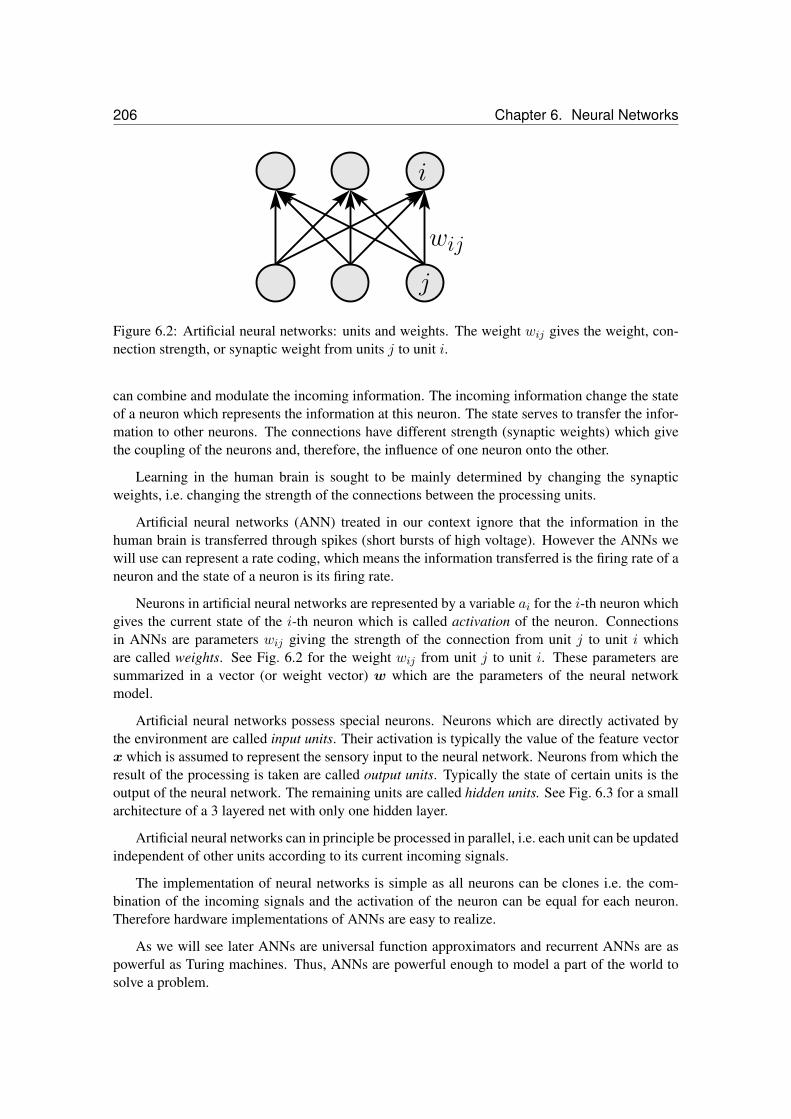
206 Chapter 6. Neural Networks
j
wij
i
Figure 6.2: Artificial neural networks: units and weights. The weight wij gives the weight, con-nection strength, or synaptic weight from units j to unit i.
can combine and modulate the incoming information. The incoming information change the stateof a neuron which represents the information at this neuron. The state serves to transfer the infor-mation to other neurons. The connections have different strength (synaptic weights) which givethe coupling of the neurons and, therefore, the influence of one neuron onto the other.
Learning in the human brain is sought to be mainly determined by changing the synapticweights, i.e. changing the strength of the connections between the processing units.
Artificial neural networks (ANN) treated in our context ignore that the information in thehuman brain is transferred through spikes (short bursts of high voltage). However the ANNs wewill use can represent a rate coding, which means the information transferred is the firing rate of aneuron and the state of a neuron is its firing rate.
Neurons in artificial neural networks are represented by a variable ai for the i-th neuron whichgives the current state of the i-th neuron which is called activation of the neuron. Connectionsin ANNs are parameters wij giving the strength of the connection from unit j to unit i whichare called weights. See Fig. 6.2 for the weight wij from unit j to unit i. These parameters aresummarized in a vector (or weight vector) w which are the parameters of the neural networkmodel.
Artificial neural networks possess special neurons. Neurons which are directly activated bythe environment are called input units. Their activation is typically the value of the feature vectorx which is assumed to represent the sensory input to the neural network. Neurons from which theresult of the processing is taken are called output units. Typically the state of certain units is theoutput of the neural network. The remaining units are called hidden units. See Fig. 6.3 for a smallarchitecture of a 3 layered net with only one hidden layer.
Artificial neural networks can in principle be processed in parallel, i.e. each unit can be updatedindependent of other units according to its current incoming signals.
The implementation of neural networks is simple as all neurons can be clones i.e. the com-bination of the incoming signals and the activation of the neuron can be equal for each neuron.Therefore hardware implementations of ANNs are easy to realize.
As we will see later ANNs are universal function approximators and recurrent ANNs are aspowerful as Turing machines. Thus, ANNs are powerful enough to model a part of the world tosolve a problem.

6.3. Linear Neurons and the Perceptron 207
input
output
hidden
Figure 6.3: Artificial neural networks: a 3-layered net with an input, hidden, and output layer.
a = wTx
x
w
Figure 6.4: A linear network with one output unit.
6.3 Linear Neurons and the Perceptron
In this section we will focus on (artificial) neural networks (NNs) which represent linear discrim-inant functions.
As in Chapter 3 we assume that objects are represented or described by feature vectors x ∈Rd. The training set consists of l objects X =
x1, . . . , xl
with a targets yi ∈ R. Again we use
the matrix of feature vectors X =(x1, . . . ,xl
)T , where X ∈ Rl×d, and the vector of targets
y =(y1, . . . , yl
)T .
The linear neural network is
g(x;w) = a = wTx . (6.1)
That means we have d input neurons where the i-th input neuron has activation xi. There is onlyone output neuron with activation a. Connections exist from each input unit to the output unitwhere the connection from the i-th input unit to the output is denoted by wi (see Fig. 6.4).

208 Chapter 6. Neural Networks
a = Wx
x
W
Figure 6.5: A linear network with three output units.
If we assume Gaussian noise, then the proper noise model is the least square error. In Chapter3 in Section 3.5.1 we treated this case and found that the optimal solution is the least squareestimator from eq. (3.98):
w =(XTX
)−1XTy . (6.2)
This solution may also be obtained by gradient descent on the empirical error function
Remp =12
l∑i=1
(yi − g(xi;w)
)2 = (6.3)
12
l∑i=1
(yi − wTxi
)2=
12
(y − X w)T (y − X w) .
The gradient is
∂
∂wRemp =
l∑i=1
(yi − wTxi
)xi = (y − X w)T X . (6.4)
The linear neuron can be extended to a linear net if the output contains more than one unit.The targets are now output vectors Y =
(y1, . . . ,yl
)T , where Y ∈ Rl×o.
The linear neural network is
g(x;w) = a = Wx , (6.5)
where W is the weight matrix W ∈ Ro×d and o is the number of output units (see Fig. 6.5 witho = 3).
For convenience the weight matrix is sometimes written as a weight vector w, where thecolumns of W are stacked on top of each other. This network is a combination of linear neuronswith
gi(x;w) = ai = wTi x , (6.6)

6.3. Linear Neurons and the Perceptron 209
where wi is the i-th line ofW written as column vector.
Because the optimal solution is
wi =(XTX
)−1XTyi , (6.7)
where yi is the i-th column of Y , we obtain as solution for the whole network
W T =(XTX
)−1XTY . (6.8)
A linear neuron with a threshold function is called perceptron. The output of the perceptron isbinary.
The perceptron model is
a = sign(wTx
), (6.9)
where sign is called threshold function. Note that the perceptron is a linear classifier from Section4.2 without an offset b. Note, that without the offset b the learning problem is not translationinvariant.
For the perceptron we assume a classification task, where y ∈ −1, 1.The error function for the perceptron is defined as
Remp = −l∑
i=1; aiyi=−1
yi wTxi . (6.10)
The error is the margin error of the support vector machine e.g. in Section 4.6 in the eq. (4.54) withb = 0 and very small ρ. The C support vector error is obtained ifw is scaled such that the minimal|wTxi| of above misclassifications is one. Scaling does not influence the perceptron output.
Using a gradient update we obtain
∆w = ηl∑
i=1; aiyi=−1
yi xi (6.11)
or in an on-line formulation
if a y = −1 : ∆w = η y x . (6.12)
The update rule is very simple: if a pattern is wrongly classified then the label multiplied by theinput vector is added to the weight vector. Fig. 6.6 depicts the perceptron update rule.
Assume that the problem is linear separable. The perceptron learning rule converges afterfinite many steps to a a solution which classifies all training examples correct.
However an arbitrary solution out of all possible solutions is chosen. If the problem in notlinearly separable then the algorithms does not stop.

210 Chapter 6. Neural Networks
x1
w
ηx
w + η x
x2
x
x
w
−ηx
w − η x
x2
x1
Figure 6.6: The perceptron learning rule. Left: a positive example is wrongly classified andcorrectly classified after the weight update. Right: a negative example is wrongly classified andcorrectly processed after weight update.
Minsky and Papert showed 1969 that many problems cannot be solved by the perceptron. Forexample the XOR problem (see Fig. 3.18) is a nonlinear problem which cannot be solved by theperceptron.
Because of the work of Minsky and Papert neural networks were not popular until the mid80ies where the multi layer perceptron with nonlinear units and back-propagation was reintro-duced.
6.4 Multi-Layer Perceptron
With the work Rumelhart et al. [1986b,a] neural networks and especially the multi-layer percep-tron trained with back-propagation became very popular.
6.4.1 Architecture and Activation Functions
A multi-layer perceptron (MLP) consists of more than one perceptron where the output of one per-ceptron is the input of the next perceptron. Further, the activation (state) of a neuron is computedthrough a nonlinear function.
We define for the multi-layer perceptron (MLP, see Fig. 6.7):
ai: activity of the i-th unit
a0 = 1: activity of 1 of the bias unit
wij : weight from unit j to unit i
wi0 = bi: bias weight of unit i
W : number of weights
N : number of units

6.4. Multi-Layer Perceptron 211
neti
wij
ai = f(neti)
j
i
L3: output
L2: hidden
L1: input
bi
Figure 6.7: Figure of an MLP.
I: number of inputs units (1 ≤ i ≤ I) located in the first layer called input layer.
O: number of output units (N − O + 1 ≤ i ≤ N ) located in the last layer called outputlayer.
H: number of hidden units (I < i ≤ N −O) located in the hidden layers.
L: number of layers, where Lν is the index set of the ν-th layer; L1 = 1, . . . , I andLL = N −O + 1, . . . , N.
neti: network input to the i-th unit (I < i) computed as
neti =N∑j=0
wij aj (6.13)
f : activation function with
ai = f(neti) (6.14)
It is possible to define different activation functions fi for different units. The activationfunction is sometimes called transfer function (in more realistic networks one can distin-guish between activation of a neuron and the signal which is transferred to other neurons).
the architecture of a neural network is given through number of layers, units in the layers,and defined connections between units – the activations function may be accounted to thearchitecture.
A feed-forward MLP has only connections from units in lower layers to units in higher layers:
i ∈ Lν and j ∈ Lν′ and ν ≤ ν ′ ⇒ wij = 0 . (6.15)

212 Chapter 6. Neural Networks
For a conventional multi-layer perceptron there are only connections or weights between con-secutive layers. Other weights are fixed to zero. The network input is then for i in layer 1 < νis
∀i∈Lν : neti =N∑
j;j∈Lν−1
wij aj . (6.16)
Connections between units in layers which are not adjacent are called shortcut connections.
The forward pass of a neural network is given in Alg. 6.1.
Algorithm 6.1 Forward Pass of an MLP
BEGIN initializationprovide input xfor all (i = 1 ; i ≤ I ; i+ +) do
ai = xiend for
END initializationBEGIN Forward Pass
for (ν = 2 ; ν ≤ L ; ν + +) dofor all i ∈ Lν do
neti =N∑
j=0;wij existswij aj
ai = f(neti)end for
end forprovide output gi(x;w) = ai, N −O + 1 ≤ i ≤ N
END Forward Pass
Activation Functions.
The commonly used activation functions are sigmoid functions.
The logistic function is
f(a) =1
1 + exp(− a)(6.17)
and the tanh activation function is
f(a) = tanh(a) =exp(a) − exp(− a)exp(a) + exp(− a)
. (6.18)
Both functions are equivalent because
12
(tanh(a/2) + 1) =1
1 + exp(− a). (6.19)

6.4. Multi-Layer Perceptron 213
(proof as exercise)
That means through weight scaling and through adjusting the bias weights the networks withlogistic or tanh can be transformed into each other.
Also quadratic or other activation functions can be used but the fact that the sigmoid functionsare squashed into a interval makes learning robust. Because the activation is bounded the deriva-tives are bounded as we see later. Networks with sigmoid activation are even more robust againstunknown input which can drive some activations in regions which are not explored in the trainingphase.
Higher order units.
Higher order units use not a linear neti. For example second order units have the form
neti =N∑
(j1,j2)=(0,0)
wij1j2 aj1 aj2 . (6.20)
Note that linear and constant terms are considered because of the bias unit a0 = 1.
We will use higher order units in Section 6.6.6 in order to gate information flow and to accesscertain information.
Symmetric Networks.
Symmetric networks can be produced with the tanh function if the signs of input weights andoutput weights are changed because tanh(−x) = − tanh(x), therefore, w2 tanh(w1 x) =(−w2) tanh((−w1) x).
Permutations of the hidden units in one layer leads to equivalent networks.
That means the same function can be represented through different network parameters.
6.4.2 Universality
The in [Funahashi, 1989] it is proven that MLPs are universal function approximators:
Theorem 6.1 (MLPs are Universal Approximators) If the activation function f is not constant,monotonic increasing, continuous, and bounded, then each continuous function g(x) on a compactinterval K can be approximated arbitrary exact through a three-layered neural network o(x;w):
maxx∈K|o(x;w) − g(x)| < ε , (6.21)
where ε is given and the number of hidden units H depend on ε and g.
This statement (neural networks are universal function approximators) was also shown in[Hornik et al., 1989, Stinchcombe and White, 1989, White, 1990].
We cite from [Hornik et al., 1989]:

214 Chapter 6. Neural Networks
In other words, standard feed-forward networks with only a single hidden layer canapproximate any continuous function uniformly on any compact set and any measur-able function arbitrarily well in the ρµ metric, regardless of the squashing function Ψ(continuous or not), regardless of the dimension of the input space r, and regardlessof the input space environment µ. Thus, Σ networks are also universal approximators.
and
In other words, there is a single hidden layer feed-forward network that approximatesany measurable function to any desired degree of accuracy on some compact set Kof input patterns that to the same degree of accuracy has measure (probability ofoccurrence) 1.
Note that in [Hornik et al., 1989] in contrast to [Funahashi, 1989] non-continuous activationfunctions are allowed.
6.4.3 Learning and Back-Propagation
To train neural network the gradient based methods from Chapter 5 can be applied.
The gradient of a neural network can be computed very efficiently by back-propagation [Rumel-hart et al., 1986b,a] which was even earlier proposed by [Werbos, 1974]. The back-propagationalgorithm made artificial neural networks popular since the mid 80ies.
In the following we derive the back-propagation algorithm in order to compute the gradient ofa neural network.
In eq. (3.161) we defined the empirical error as
Remp(w,X,Y ) =1l
l∑i=1
L(yi, g
(xi;w
)), (6.22)
where we generalized to multiple outputs. According to eq. (5.3) the gradient descent update is
wnew = wold − η ∇wRemp(w,X,Y ) . (6.23)
We obtain
∇wRemp(w,X,Y ) =1l
l∑i=1
∇wL(yi, g
(xi;w
)). (6.24)
We have to compute
∂
∂wklL(yi, g
(xi;w
))(6.25)
for all wkl.

6.4. Multi-Layer Perceptron 215
∂
∂wklL(yi, g
(xi;w
))= (6.26)
∂
∂netkL(yi, g
(xi;w
)) ∂netk∂wkl
=
∂
∂netkL(yi, g
(xi;w
))al .
We define the δ-error at unit k as
δk =∂
∂netkL(yi, g
(xi;w
))(6.27)
and obtain
∂
∂wklL(yi, g
(xi;w
))= δk al . (6.28)
The δ-error at the output units is
∀1 ≤ s ≤ O : δN−O+s = (6.29)∂
∂gsL(yi, g
(xi;w
))f ′(netN−O+s) =
∂L
∂aN−O+sf ′(netN−O+s) ,
where f ′ denotes the derivative of the activation function f .
The δ-error at units not in the output layer is
δk =∂
∂netkL(yi, g
(xi;w
))= (6.30)∑
n
∂
∂netnL(yi, g
(xi;w
)) ∂netn∂netk
=
∑n
∂
∂netnL(yi, g
(xi;w
)) ∂netn∂netk
=
f ′(netk)∑n
δn wnk ,
where the∑
n goes over all n for which wnk exists. Typically n goes over all units in the layerabove the layer where unit k is located.
This efficient computation of the δ-errors led to the term “back-propagation” because the δ-errors of one layer are used to compute the δ-errors of the layer below. The algorithm is sometimesalso called “δ-propagation”. Fig. 6.8 depicts the back-propagation algorithm for a 4-layer feed-forward network.

216 Chapter 6. Neural Networks
∑k δk wki
L3: hidden 2
L1: input
L2: hidden 1 i
k
δk
wki
δi = ∂L(y,x,w)∂ai
f ′(neti)
δi = f ′(neti)
L4: output
Figure 6.8: 4-layer MLP where the back-propagation algorithm is depicted. The δk =∂
∂netkL(yi, g
(xi;w
))are computed from the δ’s of the higher layer. The back-propagation
algorithm starts form the top layer and ends with the layer 2 where the weights to layer 2 areupdated.
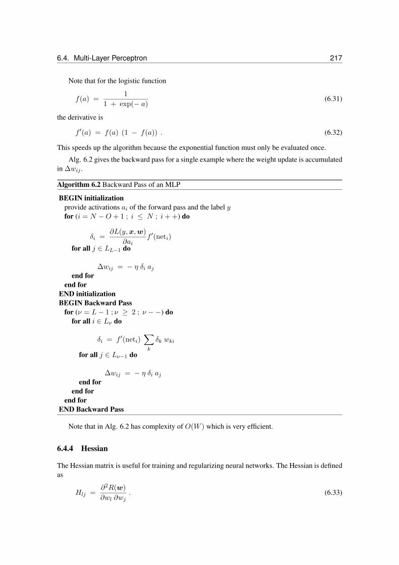
6.4. Multi-Layer Perceptron 217
Note that for the logistic function
f(a) =1
1 + exp(− a)(6.31)
the derivative is
f ′(a) = f(a) (1 − f(a)) . (6.32)
This speeds up the algorithm because the exponential function must only be evaluated once.
Alg. 6.2 gives the backward pass for a single example where the weight update is accumulatedin ∆wij .
Algorithm 6.2 Backward Pass of an MLP
BEGIN initializationprovide activations ai of the forward pass and the label yfor (i = N −O + 1 ; i ≤ N ; i+ +) do
δi =∂L(y,x,w)
∂aif ′(neti)
for all j ∈ LL−1 do
∆wij = − η δi ajend for
end forEND initializationBEGIN Backward Pass
for (ν = L− 1 ; ν ≥ 2 ; ν −−) dofor all i ∈ Lν do
δi = f ′(neti)∑k
δk wki
for all j ∈ Lν−1 do
∆wij = − η δi ajend for
end forend for
END Backward Pass
Note that in Alg. 6.2 has complexity of O(W ) which is very efficient.
6.4.4 Hessian
The Hessian matrix is useful for training and regularizing neural networks. The Hessian is definedas
Hlj =∂2R(w)∂wl ∂wj
. (6.33)

218 Chapter 6. Neural Networks
For most risk functions it is sufficient to calculate the Hessian of the loss function for one exampleto compute the Hessian the risk
Hij(yi,xi,w) =∂2L(yi,xi,w)∂wl ∂wj
. (6.34)
and then combine these derivatives. In the following we write Hij for the Hessian of the lossfunction for a certain example.
We have already seen that optimization techniques like the Newton method (see Section 5.4.1)uses the Hessian or uses characteristics of the Hessian to optimize the step-size (see Section 5.3).
Further the Hessian can be used to retrain a network or to identify units or weights which arenot needed in the architecture (see Section 6.4.5.3). In other applications the Hessian is used toassign error bars to the outputs (see Section 7.4) or to determine regularization parameters (seeSection 7.5) or to compare or average over models (see Section 7.8).
In this section we especially consider techniques which are adapted to neural networks toefficiently compute the Hessian or to approximate it.
Diagonal approximations.
According to eq. 6.26 we have
∂2L(w)∂w2
ij
=∂2L (w)∂net2
i
a2j . (6.35)
Further the chain rule gives
∂2L (w)∂net2
i
= (6.36)
(f ′(neti)
)2∑l
∑k
wlj wkj∂2L (w)
∂netl ∂netk+ f ′′(neti)
∑l
∂L (w)∂netl
≈
(f ′(neti)
)2∑l
w2lj
∂2L (w)∂net2
l
+ f ′′(neti)∑l
∂L (w)∂netl
,
where the off-diagonal elements of the Hessian were neglected.
This approximation can be done with an additional forward and backward pass and, therefore,is as efficient as back-propagation with complexity O(W ).
However the approximation is often rough because the off-diagonal elements have large abso-lute value.
Outer product / Levenberg-Marquardt Approximation.
The Levenberg-Marquardt algorithm in Section 5.5 approximated the Hessian in eq. (5.66)

6.4. Multi-Layer Perceptron 219
through
Hij,kl = (6.37)
∂2R
∂wij ∂wkl=
l∑i=1
(∂ei
∂wij
∂ei
∂wkl+ ei
∂2ei
∂wij ∂wkl
)≈
l∑i=1
∂aN (xi)∂wij
∂aN (xi)∂wkl
,
where
ei = (aN (xi;w) − yi) (6.38)
and
R(w) =l∑
i=1
(ei(w)
)2. (6.39)
Attention: that only holds for squared error!
Inverse Hessian Approximation.
We will need the inverse Hessian in Section 6.4.5.3 which can be approximated by an outerproduct approximation.
If gi is the weight gradient for example xi then
H =l∑
i=1
gi(gi)T
. (6.40)
This means the Hessian can be build sequentially
Hk =k∑i=1
gi(gi)T
, (6.41)
whereH l = H .
We obtain
Hk+1 = Hk + gk+1(gk+1
)T. (6.42)
To this formula the matrix inversion lemma
(A + B C)−1 = A−1 − A−1B(I + C A−1B
)−1C A−1 (6.43)

220 Chapter 6. Neural Networks
is applied which gives
(Hk+1
)−1=(Hk)−1 −
(Hk)−1
gk+1(gk+1
)T (Hk)−1
1 + (gk+1)T (Hk)−1gk+1
. (6.44)
Because only(Hk)−1
gk+1 must be computed. and then each component of the Hessian canbe updated, the algorithm has O(W 2) complexity per iteration.
If the initial matrix is α I then this algorithm gives the inverse of (H + α I). In manyalgorithms (H + α I) is more robust because the inversion with small eigenvalues is avoided.
If the Hessian is build up iteratively over more epochs (whole training set is updated) thenalso quasi-Newton methods (see Section 5.4.1) may be considered because they also build up anapproximation of the Hessian which improves step by step.
Finite differences.
Either finite differences can be applied to the error function or the gradient of the error function.
Because for finite differences of the error function we have to disturb each pair of weights(R(wij ± ε, wkl ± ε) and perform for each disturbance a forward pass we obtain complexity ofO(W 3).
The finite differences applied to the gradient gives
Hij,kl ≈ 12 ε
(∂R
∂wij(wkl + ε) − ∂R
∂wij(wkl − ε)
). (6.45)
This is more efficient than finite differences of the error function because only W weights have tobe disturbed and the gradient can be computed in O(W ) time by back-propagation. Therefore theHessian can be approximated in O(W 2) complexity.
Exact Computation of the Hessian.
So far only the diagonal approximation was as efficient as back-propagation with O(W ) andthe other approximations of the Hessian have complexity O(W 2).
However the Hessian can be computed exactly with complexity O(W 2). Ideas from the back-propagation are used for computing the Hessian.
From eq. (6.27) and eq. (6.28) we have
δk =∂
∂netkL(yi, g
(xi;w
))(6.46)
∂
∂wklL(yi, g
(xi;w
))= δk al .
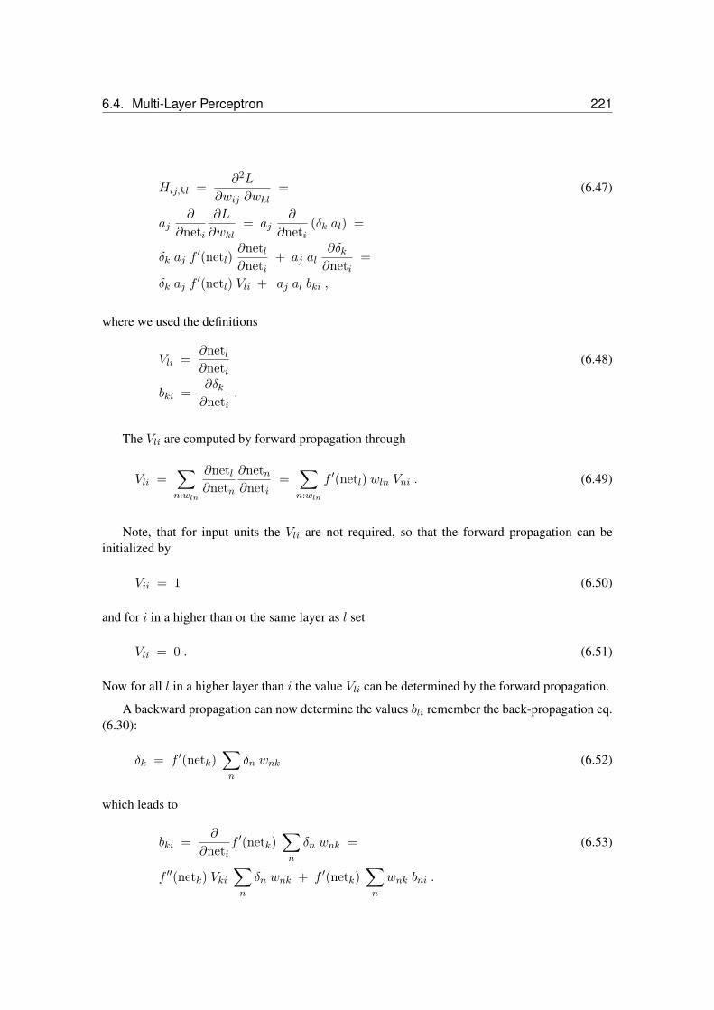
6.4. Multi-Layer Perceptron 221
Hij,kl =∂2L
∂wij ∂wkl= (6.47)
aj∂
∂neti∂L
∂wkl= aj
∂
∂neti(δk al) =
δk aj f′(netl)
∂netl∂neti
+ aj al∂δk∂neti
=
δk aj f′(netl) Vli + aj al bki ,
where we used the definitions
Vli =∂netl∂neti
(6.48)
bki =∂δk∂neti
.
The Vli are computed by forward propagation through
Vli =∑n:wln
∂netl∂netn
∂netn∂neti
=∑n:wln
f ′(netl) wln Vni . (6.49)
Note, that for input units the Vli are not required, so that the forward propagation can beinitialized by
Vii = 1 (6.50)
and for i in a higher than or the same layer as l set
Vli = 0 . (6.51)
Now for all l in a higher layer than i the value Vli can be determined by the forward propagation.
A backward propagation can now determine the values bli remember the back-propagation eq.(6.30):
δk = f ′(netk)∑n
δn wnk (6.52)
which leads to
bki =∂
∂netif ′(netk)
∑n
δn wnk = (6.53)
f ′′(netk) Vki∑n
δn wnk + f ′(netk)∑n
wnk bni .

222 Chapter 6. Neural Networks
Note that wij = wnk must be avoided in above equations because we expanded ∂∂wij
into
aj∂
∂neti. However it is always possible to use the symmetric Hessian entry because it avoids this
equality otherwise the network would contain cycles.
The initial values bki are given as
bki =∑n
Skn Vni = [SVi]k = [SV ]ki , (6.54)
where
Skj =∂2L
∂netk ∂netj. (6.55)
The initial conditions for the backward pass are for output unit i
δi =∂L(y,x,w)
∂aif ′(neti) (6.56)
and for i and j output units (where output units are not interconnected):
Sij =∂2L(y,x,w)∂ai ∂aj
f ′(neti) f ′(netj) . (6.57)
The algorithm Alg. 6.3 has complexity O(W 2) which is optimal because the Hessian hasO(W 2) entries (it is not W 2 because of symmetries).
Multiplication of the Hessian with a Vector.
Similar to previous algorithm the product of the Hessian with a vector can be computed veryefficiently. It can be computed in O(W ) time.
Following Pearlmutter [Pearlmutter, 1994] (see similar approach of Møller [Mller, 1993]) wedefine a differential operator as
R. = vT∇w (6.58)
in order to derive a efficient way to compute
vTH = R∇wL = vT∇2wL . (6.59)
We have
Rw = v (6.60)
and
Rai = 0 (6.61)
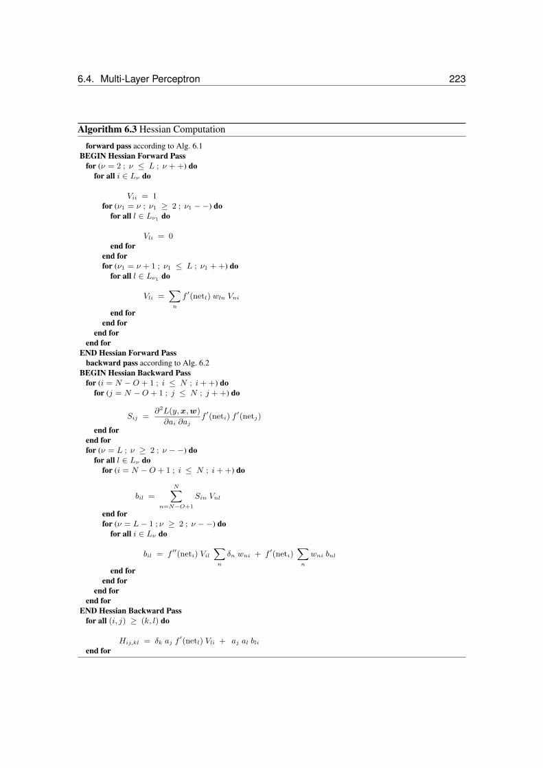
6.4. Multi-Layer Perceptron 223
Algorithm 6.3 Hessian Computation
forward pass according to Alg. 6.1BEGIN Hessian Forward Pass
for (ν = 2 ; ν ≤ L ; ν + +) dofor all i ∈ Lν do
Vii = 1for (ν1 = ν ; ν1 ≥ 2 ; ν1 −−) do
for all l ∈ Lν1 do
Vli = 0end for
end forfor (ν1 = ν + 1 ; ν1 ≤ L ; ν1 + +) do
for all l ∈ Lν1 do
Vli =Xn
f ′(netl) wln Vni
end forend for
end forend for
END Hessian Forward Passbackward pass according to Alg. 6.2
BEGIN Hessian Backward Passfor (i = N −O + 1 ; i ≤ N ; i+ +) do
for (j = N −O + 1 ; j ≤ N ; j + +) do
Sij =∂2L(y,x,w)
∂ai ∂ajf ′(neti) f
′(netj)
end forend forfor (ν = L ; ν ≥ 2 ; ν −−) do
for all l ∈ Lν dofor (i = N −O + 1 ; i ≤ N ; i+ +) do
bil =
NXn=N−O+1
Sin Vnl
end forfor (ν = L− 1 ; ν ≥ 2 ; ν −−) do
for all i ∈ Lν do
bil = f ′′(neti) VilXn
δn wni + f ′(neti)Xn
wni bnl
end forend for
end forend for
END Hessian Backward Passfor all (i, j) ≥ (k, l) do
Hij,kl = δk aj f′(netl) Vli + aj al bli
end for

224 Chapter 6. Neural Networks
for ai input unit.
We obtain
Rai = f ′(neti)Rneti (6.62)
and
Rneti =∑j
wijRaj +∑j
vij aj , (6.63)
where the first sum vanishes for j in the input layer.
Now the operator is applied to the δ’s of the back-propagation algorithm.
For an output unit i we have
δi =∂L(y,x,w)
∂aif ′(neti) (6.64)
which gives
Rδi = (6.65)(∂2L(y,x,w)
∂a2i
(f ′(neti)
)2 +∂L(y,x,w)
∂aif ′′(neti)
)Rneti
For non-output units i we have
Rδi = f ′′(neti)Rneti∑k
wki δk + (6.66)
f ′(neti)∑k
vki δk + + f ′(neti)∑k
wki Rδk
The Hessian can be computed as
R∂L
∂wij
= Rδi aj = Rδi aj + Rajδi , (6.67)
where again for the input units j the second term vanishes.
The algorithm for computing the product vTH of a vector with the Hessian has complexityO(W ).
This algorithm applied to the W unit vectors allows to extract the Hessian in O(W 2) time butAlg. 6.3 is more efficient.
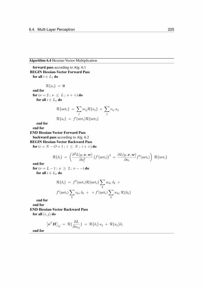
6.4. Multi-Layer Perceptron 225
Algorithm 6.4 Hessian-Vector Multiplication
forward pass according to Alg. 6.1BEGIN Hessian-Vector Forward Pass
for all i ∈ L1 do
Rai = 0end forfor (ν = 2 ; ν ≤ L ; ν + +) do
for all i ∈ Lν do
Rneti =∑j
wijRaj +∑j
vij aj
Rai = f ′(neti)Rnetiend for
end forEND Hessian-Vector Forward Pass
backward pass according to Alg. 6.2BEGIN Hessian-Vector Backward Pass
for (i = N −O + 1 ; i ≤ N ; i+ +) do
Rδi =(∂2L(y,x,w)
∂a2i
(f ′(neti)
)2 +∂L(y,x,w)
∂aif ′′(neti)
)Rneti
end forfor (ν = L− 1 ; ν ≥ 2 ; ν −−) do
for all i ∈ Lν do
Rδi = f ′′(neti)Rneti∑k
wki δk +
f ′(neti)∑k
vki δk + + f ′(neti)∑k
wki Rδkend for
end forEND Hessian-Vector Backward Pass
for all (i, j) do
[vTH
]ij
= R ∂L∂wij
= Rδi aj + Rajδiend for

226 Chapter 6. Neural Networks
6.4.5 Regularization
In Section 3.6.4 we introduced the idea of structural risk minimization, where the empirical risk(the training error) is minimized for a function class with bounded complexity.
In Section 3.6.5 the margin was define as a complexity measure and in Chapter 4 the supportvector machines minimize the complexity given as the margin for a perfect classification of thetraining data. In Section 4.4 perfect classification was replaced by margin errors and a new variableC was introduced. The variableC controlled the trade-off between margin errors and large margin.Therefore in Section 4.4 we already found the trade-off between low complexity and low trainingerror.
In Fig. 3.20 the trade-off between complexity and training error (empirical risk) is depicted:
R ≤ Remp + complexity . (6.68)
Increasing complexity leads to smaller training error but the test error, the risk, increases at somepoint.
Also Fig. 3.15 shows the relation between the test error R(g) and the training error as a func-tion of the complexity. The test error R first decreases and then increases with increasing com-plexity. The training error decreases with increasing complexity. The test error R is the sum oftraining error and a complexity term. At some complexity point the training error decreases slowerthan the complexity term increases – this is the point of the optimal test error.
For low test error, i.e. high generalization, we have to control the complexity of the neuralnetwork.
Typical regularization terms are
smoothing terms, which control the curvature and higher order derivatives of the functionrepresented by the network
complexity terms which control number of units and weights or their precision.
If the network extracts characteristics which are unique for training data only (the data pointswhich have been drawn), stem from noise, or are due to outliers in the training data then overfit-ting is present. In general all regularization terms which avoid that the network can extract suchcharacteristics from the training data can regularize. These terms allow the network only to extractthe most prominent characteristics which are not observed at one example but for many examples.
The regularization can be done
during or
after
training the network.
Regularization during training has the problem that there is a trade-off between decreasing theempirical risk and the complexity. This trade-off is difficult to regulate during learning. Advantageis that a constant pressure is on the learning to efficiently extract the structures.

6.4. Multi-Layer Perceptron 227
Regularization after training has the problem that the network can be spoiled by the trainingprocedure. Important structures may distributed over the whole network so that pruning weightsor nodes is impossible without destroying the important structure. E.g. a structure which can berepresented by a small subnetwork may be in a large architecture containing copies of this smallsubnetwork. If now one of these copies is deleted the error decreases because it contributes tothe whole output. On the other hand the subnetwork share the task of representing the impor-tant structure therefore have free capacity to represent more characteristics of the training dataincluding noise. Advantage of the regularization after training is that one can better control thecomplexity and the trade-off between empirical error and complexity.
Because all regularization must be expressed through weight values, a problem appears forall these methods. The network function can be implemented through different weight values andsome weight values may indicate lower complexity even if they implement the same function.
6.4.5.1 Early Stopping
To control the complexity of the network it is possible to stop learning before the minimum isreached. This regularization technique is called “early stopping” and belongs to regularizationafter learning. Early stopping can be seen as a training procedure which produces a sequences ofnetworks with increasing complexity. Complexity is controlled by selecting one of these networksafter learning.
During learning the network will first extract the most dominant rules, that is the most impor-tant structures in the data. Here “important” or “dominant” means that the rule can be applied orstructure is present at many training examples. These rules or structures can decrease the train-ing error most efficiently because the loss decreases for many examples. Later in the learningprocedure characteristics are found which apply only to few or just one example.
If the network is initialized with small weights and sigmoid activation functions are used, thenat the beginning of learning the network implements an almost linear function. The initial networkfunction is made more and more nonlinear during learning. For a highly nonlinear network func-tion the weights in the network must be large. This means as early the learning is stopped as morelinear the network function will be and as lower is the complexity.
In Fig. 3.15 the relation between the test error and the training error is shown. If the complexitygrows with learning time, then the test error first decreases and then increases again. Optimalwould be to stop where the test error is minimal.
To analytically determine the best stopping time is complicated. Only rough guesses can begiven and do not help in practice.
A practical way is to use a validation set besides the training set to determine the best stoppingtime. However the validation examples are lost as training examples.
Disadvantage of early stopping is that there is no pressure on the learning algorithm to focuson the most prominent structure and efficiently use the resources. Also dominant but complicatedstructures are not found because to extract them would take more time.

228 Chapter 6. Neural Networks
6.4.5.2 Growing: Cascade-Correlation
The architecture, the number of units and weights, strongly influences the complexity of the net-work. Growing algorithms start with small networks and add stepwise new units or new weightswhich amount to increasing the complexity.
We classify growing algorithms as regularization techniques after training because duringtraining no regularization is done. Regularization is obtain through selecting a network from ahierarchy of networks with increasing complexity similar to early stopping.
Well know algorithms for classification are the pocket and the tiling algorithm.
We will introduce the best known algorithm: cascade-correlation.
Cascade-correlation works as follows: If a new hidden unit k is added then first its weightsare trained to maximize the correlation between the residual error and the unit’s activation. Theobjective to maximize is
Ck =N∑
j=N−O+1
∣∣∣∣∣l∑
i=1
(ak − ak) (εj − εj)
∣∣∣∣∣ , (6.69)
where εj = (aj − yj−N+O) is the error of output unit j (εj its mean value) and ak is the activationof the new hidden unit k (ak its mean value).
The derivative of Ck with respect to the weights is just
∂Ck∂wkj
=N∑
j=N−O+1
±l∑
i=1
(εj − εj) f ′(netk) aj , (6.70)
where the sign is given by the sign of the correlation in eq. (6.69).
The training is very fast because only the incoming connections to the new hidden units haveto be trained.
The hidden to output weights are then found by a linear least-square estimate (see eq. (3.98))if the output unit(s) is (are) linear. Otherwise again a gradient descent method can be applied todetermine the hidden to output weights. Here also a single layer of weights has to be trained. Fig.6.9 shows the architecture of the cascade-correlation network.
Disadvantage of growing or “constructive” algorithms is that units or weights are added onlyin small groups. Therefore, the combined effect of units cannot be used. If for example a reductionof the error can be done only through a couple of units then this would not be detected. It is unclearwhen the error starts to decrease therefore it is hard to decide when to stop or add a new unit.
6.4.5.3 Pruning: OBS and OBD
The opposite approach to growing is pruning. With pruning first a neural network is traineduntil a local minimum of the training error (empirical risk) is found. Now the complexity oftrained network is reduced by removing weights (setting them to zero) from the network. Those

6.4. Multi-Layer Perceptron 229
hidden units
o = a5
a1 = x1
a0 = 1
a2 = x2
a3
a4
output unit
Figure 6.9: Cascade-correlation: architecture of the network. Squares are weights which aretrained whereas crosses represent weights which retrained only after the addition of a hidden unit.First the hidden unit 3 with activation a3 was added and then hidden unit 4 with activation a4.
weights are removed which do not dramatically increase the training error to ensure that the majorinformation extracted from the training data is still coded in the network.
Pruning methods are typical methods for regularization after training.
Method like in [White, 1989, Mozer and Smolensky, 1989, Levin et al., 1994] remove unitsand in [Moody, 1992, Refenes et al., 1994] even input units are removed. Before removing a unitsor a weight its importance must be measured. The importance is determined by the influence orcontribution of the unit to producing the output.
To determine the increase of the error if a weight is deleted, a Taylor expansion of the empiricalerror R(w) around the local minimum w∗ is made (that was already done in eq. (5.72). Thegradient vanishes in the minimum∇wR(w∗) = 0, therefore we obtain with ∆w = (w − w∗)
R(w) = R(w∗) +12
∆wTH(w∗) ∆w + O(
(∆w)3), (6.71)
whereH is the Hessian.
For small |∆w| the error increase R(w) − R(w∗) for w = w∗ + ∆w is determined by∆wTH(w∗) ∆w.
To delete the weight wi we have to ensure
eTi ∆w + wi = 0 , (6.72)
where ei is the unit vector with an one at the i-th position and otherwise zeros.
“Optimal Brain Damage” (OBD) LeCun et al. [1990] uses only the main diagonal of the Hes-sian which can be computed in O(W ) time as we saw through eq. (6.36). The error increase is

230 Chapter 6. Neural Networks
determined by∑i
Hii (∆wi)2 . (6.73)
If we want to remove a weight then this term should be as small as possible. At the minimum theHessian is positive definite, which means that for all v
vTH v ≥ 0 , (6.74)
therefore
eTi H ei = Hii ≥ 0 . (6.75)
Therefore the vector ∆w is chosen as
∆w = − wi ei (6.76)
so that all components except the i-th are zero. The minimal error increase is given by
miniHii w
2i (6.77)
and the weight wk with
k = arg miniHii w
2i (6.78)
is removed.
If the error increases after removal of some weights the network is retrained again until a localminimum is found.
OBD is not able to recognize redundant weights. For example if two weights performing thesame tasks which can be done by one weight alone: assume each of the two weights has value of0.5 then this may be equivalent to set one of the weights to 1 and delete the other.
OBD was successfully applied to recognize handwritten zip (postal) codes where a networkwith 10.000 parameters was reduced to 1/4 of its original size.
A method called “Optimal Brain Surgeon” (OBS) Hassibi and Stork [1993] which uses thecomplete Hessian was introduced by Hassibi & Stork. The full Hessian allows for correcting otherweights which also allows to detect redundant weights and remove redundancies. Also retrainingcan be avoided are at least made reduced.
Above Taylor expansion and the constraint of removing weight i can be stated as an quadraticoptimization problem
min∆w
12
∆wTH ∆w (6.79)
s.t. eTi ∆w + wi = 0

6.4. Multi-Layer Perceptron 231
The Lagrangian is
L =12
∆wTH ∆w + α(eTi ∆w + wi
). (6.80)
The derivative has to be zero
∂L
∂∆w= H ∆w + α ei = 0 (6.81)
which is
∆w = − αH−1 ei (6.82)
Further we have
wi = − eTi ∆w = α eTi H−1 ei = αH−1
ii (6.83)
which gives
α =wi
H−1ii
(6.84)
and results in
∆w = − wi
H−1ii
H−1 ei . (6.85)
The objective is
12
∆wTH ∆w =12w2i
H−1ii
, (6.86)
where oneH−1 vanishes withH and the other has the form eTi H−1 ei = H−1
ii .
The criterion for selecting a weight to remove is the
12w2i
H−1ii
(6.87)
and the correction is done by
∆w = − wi
H−1ii
H−1 ei . (6.88)
Exercise: Why is the expression w2i
H−1ii
always larger than or equal to zero?
An approximation technique for the inverse Hessian was given in Section 6.4.4.
Problem with OBS is that most weights may be larger than 1.0 and the Taylor expansion isnot valid because higher terms in ∆w do not vanish. However in practice OBS does also work inthese cases because higher order derivatives are small.
Heuristics to improve OBS are

232 Chapter 6. Neural Networks
checking for the first order derivative ∇wR(w∗) = 0; if the gradient is not zero then alsothe linear term can be used to determine the increase of the error
retraining after weight deletion
checking for∥∥I − H−1 H
∥∥ > β to see the quality of the approximation of the inverseHessian.
check for weight changes larger than γ (e.g. γ = 5.0), if changes appear which are largerthan γ then the weight correction should be scaled.
In general OBS will not find the smallest network because the gradient descent training wasnot forced to use the smallest architecture to solve the problems. Therefore some structures aredistributed in a larger network which avoids to prune the network to an optimal size.
6.4.5.4 Weight Decay
Now we move on to regularization during learning. In general the error function is extended by acomplexity term Ω which expresses the network complexity as a function of the weights:
R(w) = Remp(w) + λ Ω(w) . (6.89)
This has the same form as the expressions in Theorem 3.9. In Section 3.6.5 the complexity termwas expressed through the margin and the margin in turn through the weight vector. Therefore thisis the expression which is also optimized by support vector machines.
Gradient descent in now performed on this extended error term.
∇wR(w) = ∇wRemp(w) + λ ∇wΩ(w) . (6.90)
The best known term for Ω(w) is weight decay, where small absolute weights values arepreferred over large absolute weight values.
Motivation for this term as a complexity term is similar to early stopping with small weights.If a sigmoid activation function is used then small weights kept the activation in the linear range.Therefore small absolute weight values prefer linear solutions. The same argument holds forhigher order derivatives of the network function. High derivatives can only be obtained by largeweights, therefore weight decay is a bias towards linear solutions.
Different weight decay terms were suggested like a term based on the 1-norm ‖w‖1 [Han-son and Pratt, 1989] (Laplace distribution of weights in the Bayes treatment see Chapter 7), aterm based on log
(1 + wTw
)[Williams, 1994] (Cauchy distribution of weights in the Bayes
treatment see Chapter 7), or the 2-norm ‖w‖2 = wTw [Krogh and Hertz, 1992] (Gaussiandistribution of weights in the Bayes treatment see Chapter 7).
Later in Section 7.6 we will investigate how to adjust the hyper-parameter λ for the Gaussianweight distribution according to [MacKay, 1992].
All these complexity terms tend to replace large absolute weights through a couple of smallabsolute weights. For large networks also small absolute weights can lead to high nonlinearities ifthe small weights accumulate to transfer a signal.

6.4. Multi-Layer Perceptron 233
Therefore the complexity term was further developed and a threshold for large weights intro-duced [Weigend et al., 1991]. Only changes of weights near the threshold have large impact on thecomplexity term. All weights below the threshold are pushed towards zero and the weights beyondthe threshold are not further penalized and can be even made larger in order to approximate thetraining data.
The weight decay term according to [Weigend et al., 1991] is
Ω(w) =∑i
w2i /w
20
1 + w2i /w
20
, (6.91)
where w0 is the threshold value. For example w0 = 0.2.
To have more control and to better adjust the hyper-parameter λ the gradient of Ω(w) can benormalized and multiplied by the length of the gradient ∇wRemp(w) which amount to a variableweighting of the complexity term.
For an MLP the weight decay terms can be separated for each layer of weights and individualhyper-parameters given for each layer. For example the input layer can be treated separately e.g.also for selecting or ranking input variables.
6.4.5.5 Training with Noise
To regularize and to avoid that the network extracts individual characteristics of few training exam-ples either to the training examples noise is added or to networks components [Minai and Williams,1994, Murray and Edwards, 1993, Neti et al., 1992, Matsuoka, 1992, Bishop, 1993, Kerlirzin andVallet, 1993, Carter et al., 1990, Flower and Jabri, 1993].
For example Murray and Edwards [Murray and Edwards, 1993] inject white noise into theweights which results in a new complexity term. The complexity term consists of squared weightvalues and second order derivatives. However due to the second order derivatives the algorithmsis very complex.
It can be shown that noise injection is for small weight values equivalent to Tikhonov regu-larization. Tikhonov regularization penalizes large absolute higher order derivatives of the outputwith respect to the inputs and therefore highly nonlinear functions.
6.4.5.6 Weight Sharing
Nowland and Hinton [Nowlan and Hinton, 1992] propose that the weights have special preferredvalues and should be grouped. Each group of weights should have similar values.
Each group has a preferred value and a certain range which says what weights are consideredas similar. Therefore each group j is modeled by a Gaussian
G(σj , µj) =1
(2 π)1/2 σjexp
(− 1
2 σ2j
(w − µj)2
). (6.92)
Each group j has a prior size αj which estimates what percentage of weights will belong to thisgroup.

234 Chapter 6. Neural Networks
Figure 6.10: Left: example of a flat minimum. Right: example of a steep minimum.
We obtain for the probability of a weight belonging to group j
p(w | j) =αj G(σj , µj)∑k αk G(σk, µk)
(6.93)
and the probability of observing this weight value
p(w) =∑j
p(w | j) . (6.94)
The value p(w) should be maximized and we obtain for the derivative of R(w) with respectto a single weight
∂R(w)∂wi
=∂Remp(w)
∂wi+ λ
∑j
p(wi | j) (wi − µj)σ2j
. (6.95)
Also the centers µj and the variances σ2j can be adaptively adjusted during learning.
6.4.5.7 Flat Minimum Search
Another algorithm for regularization during training is the “Flat Minimum Search” (FMS) algo-rithms [Hochreiter and Schmidhuber, 1997a]. It searches for large regions in the weight spacewhere the network function does not change but the empirical risk is small. Each parameter vectorfrom this region leads to the same empirical risk. Such a region is called “flat minimum” (see Fig.6.10).
A steep minimum corresponds to a weight vector which has to be given with high precisionin order to ensure low empirical error. In contrast a flat minimum corresponds to a weight vectorwhich can be given with low precision without influencing the empirical risk. Precision is heredefined as how exact the weight vector is given in terms of intervals. For example 1.5 means theinterval [1.45, 1.55] of length 0.1 and 1.233 means the interval [1.2325, 1.2335] of length 0.001,where the later is give more precisely than the former but needs more digits to describe. The FMSalgorithm removes weights and units and reduces the sensitivity of the output with respect to theweights and other units. Therefore is can be viewed as an algorithm which enforces robustness.

6.4. Multi-Layer Perceptron 235
From the point of view of “Minimum Message Length” [Wallace and Boulton, 1968] and“Minimum Description Length” [Rissanen, 1978] fewer bits are needed to describe a flat mini-mum. That means a flat minimum corresponds to a low complexity neural network.
An error term Ω(w) describing the local flatness is minimized. This error term consists of firstorder derivatives and can be minimized by gradient methods based on Alg. 6.4.
The FMS error term is
Ω(w) =12
−L log ε+∑i,j
logN∑
k=N−O+1
(∂ak∂wij
)2
+ (6.96)
W logN∑
k=N−O+1
∑i,j
∣∣∣ ∂ak∂wij
∣∣∣√∑Nk=N−O+1( ∂ak∂wij
)2
2 ,
where ε gives the tolerable output change as Euclidian distance (output changes below ε are con-sidered to be equal).
The derivative is
∂Ω(w)∂wuv
=N∑
k=N−O+1
∑i,j
∂Ω(w)
∂(∂ak∂wij
) ∂2ak∂wij ∂wuv
(6.97)
which is with ∂ak∂wij
as new variables
∇wΩ(w) =N∑
k=N−O+1
Hk
(∇ ∂ak
∂wij
Ω(w)), (6.98)
whereHk is the Hessian of the output unit ak.
The algorithm has complexity of O(O W ) (remember that O is the number of output units).
FMS prefers as weight decay weights close to zero, especially outgoing weights from unitswhich are not required (then the ingoing weights can be given with low precision). In contrast toweight decay FMS also prefers large weight values. Especially large negative bias weights to pushthe activation of units either to zero (outgoing weights can be given with low precision. ). Otherlarge weights push activation into regions of saturation (ingoing weights can be given with lowprecision).
6.4.5.8 Regularization for Structure Extraction
Regularization of neural networks can be used to extract structures from data.
The idea to build an auto-associator network, where the input and the output should be iden-tical (see Fig. 6.11). That means an auto-associator is a network which represents the identity.Regularization ensures a low complex bottleneck which stores the information of the input forconstructing the output.

236 Chapter 6. Neural Networks
output=input
hidden=coding
input
Figure 6.11: An auto-associator network where the output must be identical to the input. Thehidden layer must code the input information to supply it to the output layer.
+0.5
+0.5
+0.5
+0.5
+0.5
+0.5
+0.5
+0.5
+0.5
+0.5
+0.5+0.5
-0.5
+0.5
-0.5
-0.5
-0.5
-0.5
-0.5
-0.5
-0.5
-0.5
-0.5
-0.5
-0.5
Figure 6.12: Example of overlapping bars. The second and fourth vertical as well as the secondhorizontal bar is active. On the right the corresponding inputs to the neural network.
However using regularization the identity must be build using a low complexity network wherealso the output must not exactly match the input. The network is forced to extract the majorstructures from the network and present them at the output – only in this way the input can begenerated sufficiently well.
In the following we show FMS applied to auto-association.
In the first task a 5× 5 pixel square contains horizontal and vertical bars. See Fig. 6.12 for anexample. A good coding strategy would be to code bars and not the single pixels.
To the input noise is added which gives training examples as shown in Fig. 6.13.
The result of the auto-associator trained with FMS is shown in Fig. 6.14. The bar structure isextracted and efficiently coded.
Now we extract structures from images of size 150 × 150 pixel with 256 grey values. Theinput to the network is a 7× 7 square of these images.
We analyze the image of a village as in Fig. 6.15. The image is black except for special white

6.4. Multi-Layer Perceptron 237
1 2 3 4 5
6 7 8 9 10
11 12 13 14 15
16 17 18 19 20
21 22 23 24 25
Figure 6.13: 25 examples for noise training examples of the bars problem where each example isa 5× 5 matrix. The white circles are positive and the black circles are negative values. The radiusof the circle is proportional to the absolute value. The values are normalized for each 5× 5 matrixso that one maximal circle is present.

238 Chapter 6. Neural Networks
1 pruned 2 pruned 3 4 5 pruned
6 pruned 7 pruned 8 9 pruned 10 pruned
11 pruned 12 13 pruned 14 pruned 15
16 pruned 17 18 19 20
21 pruned 22 23 pruned 24 pruned 25 pruned
1 pruned 2 pruned 3 4 5 pruned
6 pruned 7 pruned 8 9 pruned 10 pruned
11 pruned 12 13 pruned 14 pruned 15
16 pruned 17 18 19 20
21 pruned 22 23 pruned 24 pruned 25 pruned
input units -> hidden units hidden units -> output units
Figure 6.14: Noise bars results for FMS. Left: weights from inputs to the hidden units. Each5 × 5 square represents one hidden unit with its ingoing weights. At the upper left corner thebias weights are given. The color coding is as in Fig. 6.13 but also the bias weights is used fornormalization. Units which are marked by “pruned” have been removed by FMS. Right: weightsfrom hidden units to output units.
regions which show buildings or streets. The result is shown in Fig. 6.15. The black backgroundwith white structures was extracted by localized white spot detectors.
We analyze the image of wood cells as in Fig. 6.17. Fig. 6.18 shows the results after trainingwith FMS.
We analyze the image of wood piece with grain as shown in Fig. 6.19. The results after trainingwith FMS are shown in Fig. 6.20.
In all these experiments a regularized auto-associator was able to extract structures in the inputdata.
6.4.6 Tricks of the Trade
6.4.6.1 Number of Training Examples
According to Baum & Haussler 1989 if from
l ≥ W
εlog2
(M
ε
)(6.99)
examples a fraction (1 − ε/2) are correctly classified then a fraction of (1 − ε) of future examplesare classified correctly. Here M is the number of units.
Further they found that
dVC ≥ (M − 2) d , (6.100)

6.4. Multi-Layer Perceptron 239
Figure 6.15: An image of a village from air.
1 pruned
6 pruned
11 pruned
16
21
2 pruned
7
17 pruned
22
3
8 pruned
1312
18 pruned
23 pruned
4 pruned
9
14 pruned
19 pruned
24 pruned
5 pruned
10
15
20 pruned
25 pruned
1 pruned 2 pruned 3 4 pruned 5 pruned
6 pruned
11 pruned
16
21
7
12
17 pruned
22
8 pruned
13
18 pruned
23 pruned
9
19 pruned
24 pruned
10
15
20 pruned
25 pruned
14 pruned
input units -> hidden units hidden units -> output units
Figure 6.16: Result of FMS trained on the village image. Left: weights from input units to hiddenunits. The most units are deleted. Right: weights from hidden units to output units.

240 Chapter 6. Neural Networks
Figure 6.17: An image of wood cells.
1 pruned 2 pruned 3 pruned 4 pruned 5 pruned
6
11 pruned
16 pruned
21
7
12 pruned
17 pruned
22 pruned
8 pruned
13
18 pruned
23
9
19 pruned
24
10
15
20
25 pruned
14
1 pruned
6
11 pruned
16 pruned
21
2 pruned
7
17 pruned
22 pruned
3 pruned
8 pruned
1312 pruned
18 pruned
23
4 pruned
9
14
19 pruned
24
5 pruned
10
15
20
25 pruned
input units -> hidden units hidden units -> output units
Figure 6.18: Result of FMS trained on the wood cell image. Left: weights from input units tohidden units. The most units are deleted. Right: weights from hidden units to output units.
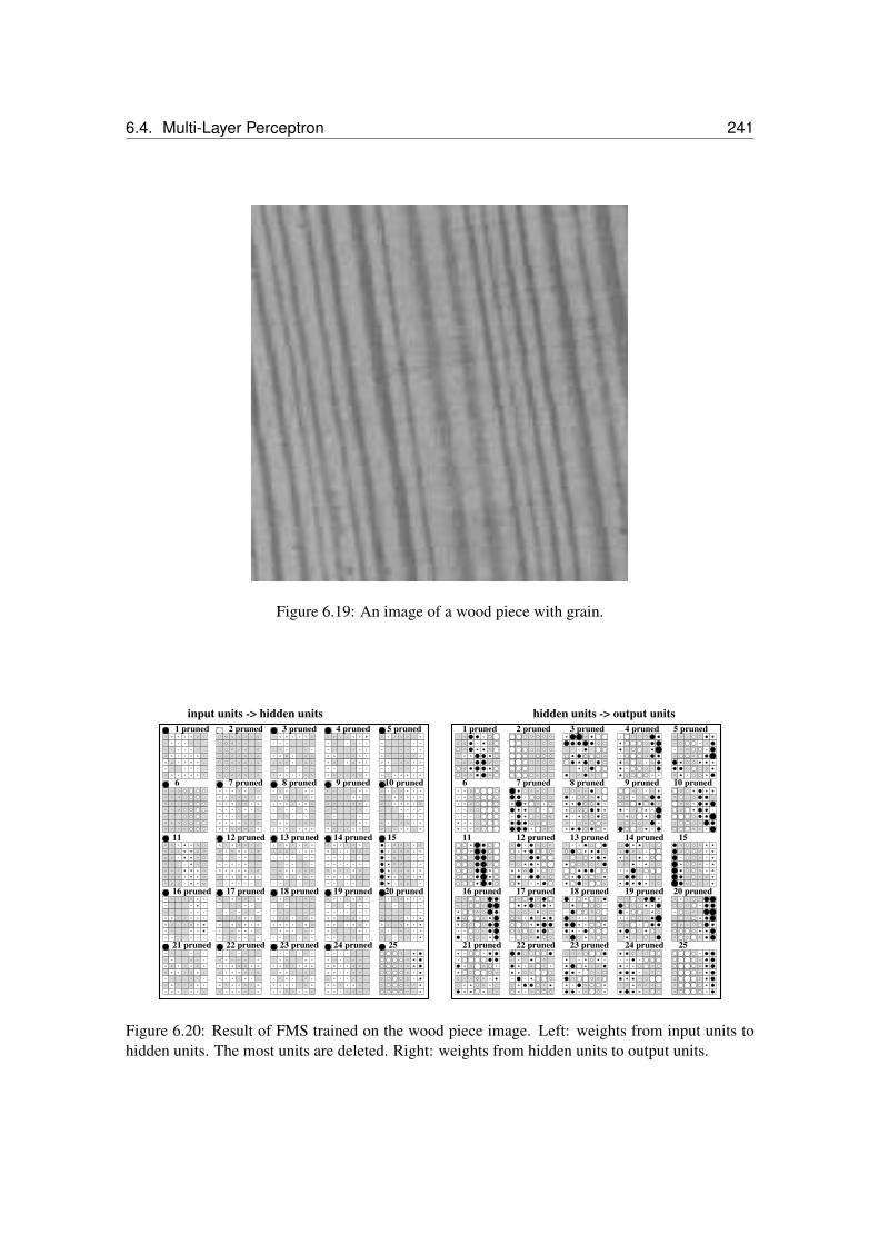
6.4. Multi-Layer Perceptron 241
Figure 6.19: An image of a wood piece with grain.
1 pruned 2 pruned 3 pruned 4 pruned 5 pruned
6
11
16 pruned
21 pruned
7 pruned
12 pruned
17 pruned
22 pruned
8 pruned
13 pruned
18 pruned
23 pruned
9 pruned
19 pruned
24 pruned
10 pruned
15
20 pruned
25
14 pruned
1 pruned
6
11
16 pruned
21 pruned
2 pruned
7 pruned
17 pruned
22 pruned
3 pruned
8 pruned
13 pruned12 pruned
18 pruned
23 pruned
4 pruned
9 pruned
14 pruned
19 pruned
24 pruned
5 pruned
10 pruned
15
20 pruned
25
input units -> hidden units hidden units -> output units
Figure 6.20: Result of FMS trained on the wood piece image. Left: weights from input units tohidden units. The most units are deleted. Right: weights from hidden units to output units.
242 Chapter 6. Neural Networks
where d is the number of inputs. For a two-layered network with one output unit we have d (M −d− 1) weights from input to the (M − d− 1) hidden units, (M − d− 1) weight from the hiddenunits to the output, (M − d− 1) hidden bias weights, and a output bias which gives
W = (d+ 2) (M − d− 1) + 1 . (6.101)
Approximatively we have
W = M d . (6.102)
For ε = 0.1 we have
l ≥ W/ε = 10 W . (6.103)
That amount to 10 times more examples than weights in the network.
6.4.6.2 Committees
In many application the performance is more robust if over different networks is averaged.
Let gj the function which is represented by the j-th network then as an committee output withC members we obtain
g(x) =1C
C∑j=1
gj(x) . (6.104)
We assume that
gj(xi) = yi + εij , (6.105)
where εj is distributed with zero mean E(εj) = 0 for each j and with zero covariance E(εj εk) =0. We further assume that all εj follow the same distribution for all j.
The expected error of the committee is
E
1C
C∑j=1
gj(x) − y
2 = E
1C
C∑j=1
(gj(x) − y)
2 = (6.106)
E
1C
C∑j=1
εj
2 =1C2
C∑j=1
E(ε2j)
=
1C
E(ε2j),
where E(ε2j
)is the error obtained by a single network.

6.4. Multi-Layer Perceptron 243
That means the error was reduced by a factor of 1C because the individual error are averaged
out.
However that does not work in practice because the errors of the individual networks are notde-correlated. In the worst case all networks converge to the same minimum and no improvementis obtained.
If the error correlation matrix is known then a weighted average
g(x) =C∑j=1
αj gj(x) (6.107)
with∑C
j=1 αj = 1 is possible. The αj can be determined by using the correlation matrix.
6.4.6.3 Local Minima
In principle are the optimization techniques for neural networks prone to finding only local minimaof the empirical error and not its global minimum.
However in practice large enough networks never get stuck in local minima because the em-pirical error can be minimized until it reaches zero, i.e. all training examples are perfectly learned.
More problematic is structural risk minimization where the risk is the empirical error plus acomplexity term. Here most sensitive is the adjustment of the hyper-parameter which scales thecomplexity term.
The only way to find a good solution is to use a simple complexity term which has not manyoptima in itself and to explore different regions in weight space.
The best approach will be treated later in Section 7.8 where the optimum of the risk is foundby monte carlo sampling.
6.4.6.4 Initialization
Initialization with small weights is to prefer because of three reasons. First the network starts withsimple functions which are almost linear. Secondly the derivatives are large in the linear activationrange compared to ranges with saturation of the units. Thirdly, weights around zero have onaverage the minimal distance to their optimal values if we assume a zero mean distribution of thefinal weight values.
Typical initialization values may be uniformly in [−0.1; 0.1].
Sometimes bias weights can have special treatment for initialization. The bias weight to theoutput can be adjusted that the output unit supplies the mean target value at the beginning oflearning.
Bias weights to hidden units can be staged so that the hidden units are not used all at once anddoing the same job. Ideally the hidden unit with the smallest negative bias is used first and thenthe second smallest and so on.
The negative bias can also be used for regularization because some units are kept away fromprocessing the output and only if there is enough error flowing back they come into the game.

244 Chapter 6. Neural Networks
6.4.6.5 δ-Propagation
During training different training examples have different contribution to the weight update. Thecontribution of few examples is sometimes important.
To speed up learning the training examples with empirical error smaller than δ are markedand not used for training in the next epochs. After certain number of epochs a sweep through alltraining examples is made and again the examples with error smaller than δ are marked and notused in the next epochs.
6.4.6.6 Input Scaling
All input components should be scaled so that they are within [−1, 1] which is the activation rangeof standard units. Larger input values lead to large weight updates and unstable learning.
Often each input component is normalized to zero mean and variance 1.
If for a input component positive and negative values express different facts then this shouldbe kept and normalization to zero mean should be avoided.
If a input component contains outliers that is extreme large absolute values then these valuesshould be mapped to a maximum or a squashing function should be used. For example if forexamples the value of one component is in [−1, 1] and one example has a value of 100 of thiscomponent, then after scaling the component is for all except one value in [−0.01, 0.01] and learn-ing of this component is difficult. Also the weight update of the large value is 100 times largerthan any other update for equal delta-error at an unit in the first hidden layer. That means oneexample overwrites the information of many other examples.
6.4.6.7 Targets
For classification it is sometimes useful to use targets of 0.2 and 0.8 for sigmoid activation in [0; 1]instead of 0 and 1 or targets of -0.8 and 0.8 for sigmoid activation in [−1; 1] instead of -1 and1. Problem with targets at the boundary of the activation interval is that some examples may getstuck in saturated regions and the derivatives are small. In this case a wrongly classified exampletakes a long time to be made correctly.
For a multi-class network it is useful to define an output unit for each class which obtains 1 astarget if the input belongs to the according class and zero otherwise.
If in a classification task the size of the classes is different then it can help to assign higheroutputs to classes with few members so that the overall error contribution is similar for all classes.
6.4.6.8 Learning Rate
Typical learning rates per example are 0.1 or 0.01. In batch learning the learning rate must bedivided by the number of examples in the training set.
However in batch learning the learning rate can be increased again because error signals getsuperimposed and the accumulative update signal is not the sum of all absolute update values. Theupdates for one weight are positive and negative depending on the example.

6.4. Multi-Layer Perceptron 245
6.4.6.9 Number of Hidden Units and Layers
In many practical applications it was of advantage to have more hidden units in a layer than outputand input units.
A network with two hidden layers is appropriate for many tasks.
Shortcut connections should be avoided because these connections obtain a larger error signal(see Section 6.6.5) and start oscillate so that the between layer weights are hard to adjust.
For some applications it is useful to reduce the activation of the constant bias unit to 0.1because its outgoing weights obtain the largest update signal and begin to oscillate.
6.4.6.10 Momentum and Weight Decay
In Section 5.2 the momentum term was introduced which in most cases help to speed up theback-propagation algorithm.
For regularization weight decay method is easy to realize.
6.4.6.11 Stopping
When should learning be stopped?
With regularization the empirical error may converge to a constant value which indicates thatlearning can be stopped.
Without regularization the empirical error may decrease by a certain rate to zero.
It is often interesting to know the maximal deviation of the output from the target value overthe training examples. If the maximal deviation is below a threshold then learning can be stopped.
Other stopping criterion include the maximal weight change of the last epochs, the error im-provement of the last epochs.
6.4.6.12 Batch vs. On-line
In many application learning can be sped up by using an on-line update (see Section 5.8), thatmeans after each example the weights are immediately changed.
Here it is important to shuffle the training examples after each epoch in order to avoid updateloops which make no progress.
Advantage of the on-line method is that all future examples see the weight update and arenot evaluated on the old weights (e.g. the bias weight to the output may be adjusted after a fewtraining examples and all other see the new bias weight.). On-line learning together with shufflingalso includes a small random effect which helps to explore the local environment in weight space.

246 Chapter 6. Neural Networks
input
weights
k
αkj
output
φj
Figure 6.21: A radial basis function network is depicted. Inputs activate the Gaussians accordinghow close the input is to the center. For the current input (dark point) the dark Gaussians areactivated.
6.5 Radial Basis Function Networks
In contrast to the neural networks which we treated so far, the support vector machines wherelocal approximators in the sense that training examples are used as a reference to classify new datapoints.
Local approximators also exist in the neural network literature, where the best known approachis radial basis function (RBF) networks.
Assume we have C basis functions φ then the RBF network is
gk(x) =C∑j=1
αkj φj (‖x − µj‖) + αk0 . (6.108)
For example Gaussian radial basis functions are
φj (‖x − µj‖) = exp
(− 1
2 σ2j
‖x − µj‖2). (6.109)
Fig. 6.21 depicts how RBF networks are working.
The parameters of this network are the weighting coefficients αkj , the centersµj and the widthσj .
It is possible to use a covariance matrix
φj (‖x − µj‖) = exp(− 1
2(x − µj)
T Σ−1j (x − µj)
). (6.110)

6.5. Radial Basis Function Networks 247
6.5.1 Clustering and Least Squares Estimate
To adjust the parameters of RBF networks there exist different approaches.
First we consider a two-stage procedure, where the in the first stage µj and σj are determinedand then the parameters αkj .
In the first stage µj and σj can be found by unsupervised methods like clustering or densityestimation (mixture of Gaussians) as will be discussed in sections 10.6 and 10.6.1.
The values φj (‖x − µj‖) are then given for the training set and can be summarized in thevector which can be expanded to a matrix Φ which also summarizes all training examples.
The parameters αkj can be summarized in the matrix Λ and the targets yj are summarized inthe vector y and the targets over the whole training set in the matrix Y .
We obtain
Y = Λ Φ (6.111)
which can be solved by a least-square estimate according to eq. (3.98) if a squared error is used:
ΛT =(ΦTΦ
)−1ΦTY . (6.112)
6.5.2 Gradient Descent
Of course the RBF networks can be trained by gradient based methods. For the mean squared errorwe have L(g(x),y) =
∑k (gk(x) − yk)
2 and if spherical Gaussians are use, the derivativesare
∂L(g(x),y)∂αkj
= (gk(x) − yk) φj = (gk(x) − yk) = (6.113)
exp
(− 1
2 σ2j
‖x − µj‖2)
∂L(g(x),y)∂σj
=∑k
(gk(x) − yk) αkj
exp
(− 1
2 σ2j
‖x − µj‖2)‖x − µj‖2
σ3j
∂L(g(x),y)∂µjl
=∑k
(gk(x) − yk) αkj
exp
(− 1
2 σ2j
‖x − µj‖2)
(xl − µjl)σ2j
.

248 Chapter 6. Neural Networks
6.5.3 Curse of Dimensionality
A compact region grows exponentially with d in a d-dimensional space. If we assume a cubewhere each axis is divided into k intervals then we obtain kd small hypercubes. This fact is knownas the “curse of dimensionality” [Bellman, 1961].
Therefore also the number of basis function should increase exponentially with dwhich in turnleads to complex models which are likely to overfit. According to [Stone, 1980], the number oftraining examples has to increase exponentially with the number of dimensions in order to ensurethat an estimator also performs well for higher dimensional data.
That means RBF networks are not suited for high-dimensional data – similar statement holdsfor other local approximation methods.
Local approximation methods must assign a value to each region in space based on local infor-mation. However, if there is no local information then local methods fail to assign an appropriatevalue to data point at this region.
6.6 Recurrent Neural Networks
Until now we only considered neural networks with feed-forward connections, i.e. the directedconnections did not form a loop. Without a loop there is a forward pass which can use the inputvariables to activate the network and produce output values.
Real neural networks however possess loops which serve to store information over time. Thatmeans the new activation depends on the old activation of the network.
The feed-forward network can be considered as a function which maps the input vector x toan output vector g(x).
Neural networks with loops, the so-called recurrent networks, map an input sequence
(x(1), . . . ,x(t), . . . ,x(T ))
to an output sequence (g(1), . . . , g(t), . . . , g(T )), where
g(t) = g (a0,x(1), . . . ,x(t)) , (6.114)
where a0 is the initial activation of the network. The index t of the sequence elements is oftencalled “time” because recurrent networks are often used to time series prediction. Also feed-forward networks can be used for time series prediction if an input vector is build of the currentinput together with past inputs. However such networks with an input window of the time seriescannot see information outside the window and their complexity (number of parameters) increaseswith window size. Recurrent networks can process long sequences with few parameters and canuse past information to optimally process information which they will see in the future sequence.
Fig. 6.22 shows an architecture of a recurrent network and Fig. 6.23 shows how a sequencesis processed.
In bioinformatics recurrent networks are however used for sequence processing.

6.6. Recurrent Neural Networks 249
L3: output
L2: recurrent
L1: input
hidden
Figure 6.22: An architecture of a recurrent network. The recurrent hidden layer is fully connected,i.e. all units are interconnected. The hidden units are able to store information, i.e. informationfrom previous inputs is kept in the hidden units.
The loops are used to store information from the previous time steps because the old activationof a unit can influence the new activation of other units or its own new activation. For examplea unit which gets activated can keep this activation by a strong positive self-recurrent connection.Such a unit can therefore store the occurrence of an event.
The computational power of recurrent networks is that of Turing machines [Siegelmann andSontag, 1991, Sun et al., 1991, Siegelmann, 1995].
6.6.1 Sequence Processing with RNNs
The activation functions and network inputs are now time dependent and are computed from theactivations of previous time step:
neti(t) =N∑j=0
wij aj(t− 1) (6.115)
ai(t) = f(neti(t)) . (6.116)
Further we need initial activations ai(0) from which are the activations before the network seesthe first input element.
Some of the units can be defined as input and some as output units.
For learning, for each input sequence (x(1), . . . ,x(t), . . . ,x(T )), a target sequence (y(1), . . . ,y(t), . . . ,y(T ))is given. We denote by x(t) the sequence (x(1), . . . ,x(t)) and by y(t) the sequence (y(1), . . . ,y(t)).
Similar to feed-forward networks we define the empirical error as
∇wRemp(w, X(T ), Y (T )) = (6.117)
1l
l∑i=1
T∑t=1
∇wL(yi(t), g
(xi(t);w)) .

250 Chapter 6. Neural Networks
A V D A A A E K V F KT
0 1 0 0 0 0 0 0 0 1 00
input sequence
target sequence
processing direction
1 t T
Figure 6.23: The processing of a sequence with a recurrent neural network. At each step thecurrent input element is fed to the input units and the output unit should supply the target value.
The next subsections discuss how recurrent networks can be learned.
6.6.2 Real-Time Recurrent Learning
For performing gradient descent we have to compute
∂
∂wuvL(yi(t), g
(xi(t);w)) (6.118)
for all wuv.
Using the chain rule this can be expanded to
∂
∂wuvL(yi(t), g
(xi(t);w)) = (6.119)∑k,k output unit
∂
∂ak(t)L(yi(t), g
(xi(t);w)) ∂ak(t)∂wuv
.
For all units k we can compute
∂ak(t+ 1)∂wuv
= f ′(netk(t+ 1))
(∑l
wkl∂al(t)∂wuv
+ δkuav(t)
), (6.120)

6.6. Recurrent Neural Networks 251
input(t) hidden(t− 1) output(t− 2)
Figure 6.24: Left: A recurrent network. Right: the left network in feed-forward formalism, whereall units have a copy (a clone) for each times step.
where δ is the Kronecker delta with δku = 1 for k = u and δku = 0 otherwise.
If the values ∂ak(t)∂wuv
are computed during a forward pass then this is called real time recur-rent learning (RTRL) [Werbos, 1981, Robinson and Fallside, 1987, Williams and Zipser, 1989,Gherrity, 1989].
RTRL has complexity of O(W 2) for a fully connected network, where W = N (N − I) =O(N2) (each unit is connected to each other unit except the input units, which do not have ingoingconnections).
Note that RTRL is independent of the length of the sequence, therefore RTRL is local in time.
6.6.3 Back-Propagation Through Time
A recurrent network can be transformed into a feed-forward network if for each time step a copyof all units is made. This procedure of unfolding in time is depicted in Fig. 6.24 for one step andthe network unfolded over the whole time is depicted in Fig. 6.25.
After re-indexing the output by adding two time steps and re-indexing the hidden units byadding one time step we obtain the network from Fig. 6.26.
To the network of Fig. 6.26 can now be trained by standard back-propagation. This method iscalled back-propagation through time (BPTT) [Williams and Zipser, 1992, Werbos, 1988, Pearl-mutter, 1989, Werbos, 1990].
We have
L(yi, g
(xi;w)) =T∑t=1
L(yi(t), g
(xi(t);w)) (6.121)
for which we write for short
L =T∑t=1
L(t) . (6.122)

252 Chapter 6. Neural Networks
...... ... ... ... ... ...
input(1) hidden(0) output(−1)
input(T + 2) hidden(T + 1) output(T )
Figure 6.25: The recurrent network from Fig. 6.24 left unfolded in time. Dummy inputs at time(t + 1) and (t + 2) and dummy outputs at (t − 2) and (t − 1) are used. The input is shifted twotime steps against the output to allow the input information be propagated through the network.

6.6. Recurrent Neural Networks 253
...... ... ... ... ... ...
input(1) hidden(1) output(1)
input(T + 2) hidden(T + 2) output(T + 2)
Figure 6.26: The recurrent network from Fig. 6.25 after re-indexing the hidden and output.

254 Chapter 6. Neural Networks
The delta error is
δj(t) = − ∂L
∂(netj(t))= −
∂(∑T
τ=t L(τ))
∂(netj(t))(6.123)
The back-propagation algorithm starts with
δj(T ) = f ′(netj(T ))∂L(T )∂aj(T )
, (6.124)
where in above reformulation T has to be replaced by (T + 2).
For t = T − 1 to t = 1:
δj(t) = f ′j(netj(t))
(∂L(t)∂aj(t)
+∑l
wljδl(t+ 1)
), (6.125)
where ∂L(t)∂aj(t)
accounts for the immediate error and the sum for the back-propagated error. Bothtypes of error occur if output units have outgoing connections. In out architecture in Fig. 6.26these errors are separated.
The derivative of the loss with respect to a weight in a layer t of the unfolded network in Fig.6.26 is
− ∂L
∂wjl(t)= − ∂L
∂(netj(t))netj(t)∂wjl(t)
= δj(t) al(t− 1) . (6.126)
Because the corresponding weights in different layers are identical, the derivative of the losswith respect to a weight is
∂L
∂wjl=
T∑t=1
∂L
∂wjl(t)= −
T∑t=1
(δj(t) al(t− 1)) . (6.127)
The on-line weight update is
wnewjl = wold
jl − η∂L
∂wjl, (6.128)
where η is the learning rate.
The complexity of BPTT is O(T W ). BPTT is local in space because its complexity per timestep and weight is independent of the number of weights.
A special case of BPTT is truncated BPTT called BPTT(n), where only n steps is propagatedback. For example n = 10 is sufficient because information further back in time cannot be learnedto store and to process (see Subsection 6.6.5).
Therefore BPTT is in most cases faster than RTRL without loss of performance.

6.6. Recurrent Neural Networks 255
6.6.4 Other Approaches
We did not consider continuous time networks and did not consider attractor networks like theHopfield model or Boltzmann machines.
These approaches are currently not relevant for bioinformatics. Continuous time networksmay be useful for modeling that is for systems biology.
In the review [Pearlmutter, 1995] a nice overview over recurrent network approaches is given.The first approach were attractor networks for which gradient based methods were developed[Almeida, 1987, Pineda, 1987].
Other recurrent network architectures are
Networks with context units which use special units, the context units, to store old activa-tions. “Elman networks” [Elman, 1988] use as context units the old activations of hiddenunits. “Jordan networks” [Jordan, 1986] use as context units old activations of the outputunits.
Special context units with time constants allow fast computation or to extract special infor-mation in the past. The “focused back-propagation” method [Mozer, 1989] and the methodof [Gori et al., 1989] introduce delay factors for the context units and lead to fast learningmethods.
Other networks directly feed the output back for the next time step [Narendra and Parthasarathy,1990] or NARX networks [Lin et al., 1996].
Local recurrent networks use only local feedback loops to store information [Frasconi et al.,1992]
Networks can be build on systems known from control theory like “Finite Impulse ResponseFilter” (FIR) networks [Wan, 1990] where at the ingoing weights a FIR filter is placed. Thearchitecture in [Back and Tsoi, 1991] uses “Infinite Impulse Response Filter” (IIR) filterinstead of FIR filter.
Other networks use “Auto Regressive Moving Average” (ARMA) units.
“Time Delay Neural Networks” (TDNNS) [Bodenhausen, 1990, Bodenhausen and Waibel,1991] use connections with time delays, that means the signal is delayed as it gets trans-ported over the connection. Therefore old inputs can be delayed until they are needed forprocessing.
The “Gamma Memory” model [de Vries and Principe, 1991] is a combination of TDNNand time constant based methods.
Recurrent network training can be based on the (extended) Kalman filter estimation [Matthews,1990, Williams, 1992, Puskorius and Feldkamp, 1994].
A variant of RTRL is “Teacher Forcing-RTRL” if the output units also have outgoing connec-tions. With “Teacher Forcing-RTRL” the activation of the output units is replaced by the targetvalues.

256 Chapter 6. Neural Networks
RTRL and BPTT can be combined to a hybrid algorithm [Schmidhuber, 1992a] which hascomplexity O(W N). Here BPTT is made for N time steps having complexity O(W N) where-after a single RTRL update is made which as complexity O(W 2/N) = O(W N).
6.6.5 Vanishing Gradient
The advantage of recurrent network over feed-forward networks with a window is that they can inprinciple use all information in the sequence which was so far processed.
However there is problem in storing the relevant information over time. If recurrent networksare not able to store information over time then there great advantage over other approaches is lost.
Consider an error signal δu(t) which is computed at time t at unit u and which gets propagatedback over q time steps to unit v. The effect of δu(t) on δv(t− q) can be computed as
∂δv(t− q)∂δu(t)
=
f ′ (netv(t− 1)) wuv q = 1
f ′ (netv(t− q))∑N
l=I∂δl(t−q+1)∂δu(t) wlv q > 1
. (6.129)
If we set lq = v and l0 = u then we obtain
∂δv(t− q)∂δu(t)
=N∑l1=I
. . .
N∑lq−1=I
q∏r=1
f ′ (netlr(t− r)) wlrlr−1 . (6.130)
Because of
δv(t− q) = − ∂L
∂netv(t− q) = −∑l
∂L
∂netl(t)∂netl(t)
∂netv(t− q) = (6.131)
∑l
δl(t)∂netl(t)
∂netv(t− q)
holds
∂δv(t− q)∂δu(t)
=∂netu(t)
∂netv(t− q) (6.132)
true.
This leads to
∂L(t)∂wij(t− q) = (6.133)∑l:output unit
f ′(netu(t))∂L(t)∂aj(t)
∂netl(t)∂neti(t− q)
∂neti(t− q)∂wij(t− q) =
∑l:output unit
f ′(netu(t))∂L(t)∂aj(t)
∂ϑi(t− q)∂ϑl(t)
aj(t− q)

6.6. Recurrent Neural Networks 257
which shows that ∂L(t)∂wij(t−q) is governed by the factor in eq. (6.130).
The eq. (6.130) contains N q−1 terms of the form
q∏r=1
f ′ (netlr(t− r)) wlrlr−1 . (6.134)
If the multipliers
f ′ (netlr(t− r)) wlrlr−1 > 1 , (6.135)
the learning is instable because derivatives grow over time and the weight update are too large.
If the multipliers
f ′ (netlr(t− r)) wlrlr−1 < 1 , (6.136)
then we have the case of vanishing gradient which means that ∂L(t)∂wij(t−q) decreases with q expo-
nentially to zero.
That means inputs which are far in the past do not influence the current loss and will not beused to improve the network. Therefore the network is not able to learn to store information in thepast which can help to reduce the current loss.
6.6.6 Long Short-Term Memory
From previous considerations we know that to avoid both instable learning and the vanishinggradient, we have to enforce
f ′ (netlr(t− r)) wlrlr−1 = 1 . (6.137)
For simplicity we consider only one unit j with a self-recurrent connection wjj and obtain
f ′ (netj(t− r)) wjj = 1 . (6.138)
Solving this differential equation gives:
f(x) =1wjj
x . (6.139)
Because f depends on the self-recurrent connection we can set wjj = 1 to fix f and obtain
f(x) = x . (6.140)
Fig. 6.27 shows the single unit which ensures that the vanishing gradient is avoided. Becausethis unit represents the identity it is immediately clear that information is stored over time throughthe architecture.

258 Chapter 6. Neural Networks
1.0
Figure 6.27: A single unit with self-recurrent connection which avoids the vanishing gradient.
1.0
Figure 6.28: A single unit with self-recurrent connection which avoids the vanishing gradient andwhich has an input.
However it is not enough to avoid the vanishing gradient and therefore ensure keeping ofinformation. A signal must be stored in the unit before it is kept. Fig. 6.28 shows the single unitwith an additional input.
However a new problem appears: all information flowing over the input connection is stored.All information which is stored gets superimposed and the single signals cannot be accessed. Moreserious, not only relevant but also all irrelevant information is stored.
Only relevant information should be stored. In order to realize that a input gate ain (basicallya sigma-pi unit) is used. If we further assume that the network input netc to the single unit issquashed the we obtain following dynamics:
a(t+ 1) = a(t) + ain(t) g (netc(t)) , (6.141)
If ain is a sigmoid unit active in [0, b] then in can serve as a gating unit.
Now we assume that the output from the storing unit is also squashed by a function h. Furtherwe can control the access to the stored information by an output gate aout which is also a sigmoidunit active in [0, b].
The memory access dynamics is
ac(t+ 1) = aout(t) h (a(t+ 1)) . (6.142)
The whole dynamics is
ac(t+ 1) = aout(t) h (a(t) + ain(t) g (netc(t))) . (6.143)

6.6. Recurrent Neural Networks 259
DA
AT
AE
VK
AV
KF
1.0
g ac = aout h(a)
ain aout
ha = a + ain g(netc)netc
netin netout
Figure 6.29: The LSTM memory cell. Arrows represent weighted connections of the neural net-work. Circles represent units (neurons), where the activation function (linear or sigmoid) is indi-cated in the circle.
The sub-architecture with the gate units ain and aout and the single unit a is called memorycell and depicted in Fig. 6.29.
The input to the storing unit is controlled by an “input gating” or attention unit (Fig. 6.29, unitmarked “ain”) which blocks class-irrelevant information, so that only class-relevant informationis stored in memory. The activation of attention units is bounded by 0 and b, i.e. the incominginformation netc(t) is squashed by a sigmoid function g. The output of the memory cell (Fig.6.29, center) is bounded by the sigmoid function h (Fig. 6.29, unit labeled as “h”). Memoryreadout is controlled by an “output gate” (Fig. 6.29, unit labeled “aout”). The cell’s output ac isthen computed according to eq. (6.142) and eq. (6.143).
The recurrent network build from memory cells is called “Long Short-Term Memory” (LSTM,[Hochreiter and Schmidhuber, 1997b]) is an RNN with a designed memory sub-architecture called“memory cell” to store information.
Memory cells can in principle be integrated into any neural network architecture. The LSTMrecurrent network structure as depicted in Fig. 6.30.
The LSTM network is well suited to protein and DNA analysis. For example it excelled inprotein classification. Here the input can be not a single amino acid or nucleotide but a wholewindow over the current position. In this case LSTM is able to learn profiles as depicted in Fig.6.31.
Using these profiles LSTM was able to generate new motives which were unknown to thePROSITE motif data base.
Currently LSTM is used for alternative splice site detection, nucleosome position detection,protein classification, etc.

260 Chapter 6. Neural Networks
output unitce
ll
cell
mem
ory
A V D A A A E K V F KT
mem
ory
Figure 6.30: LSTM network with three layers: input layer (window of the amino acid sequence– shaded elements), hidden layer (with memory cells – see Fig. 6.29), and output layer. Arrowsrepresent weighted connections; the hidden layer is fully connected. The subnetworks denotedby “memory cell” can store information and receive three kinds of inputs, which act as patterndetectors (input→ hidden), as storage control (recurrent connections), and as retrieval control (re-current connections). The stored information is combined at the output. The amino acid sequenceis processed by scanning the sequence step by step from the beginning to the end.

6.6. Recurrent Neural Networks 261
D2.5
D−0.3
D−1.2
D−1.7
D1.7
D0.2
R1.2
A0.1
A1.8
A0.2
A−0.6
A0.9
A−0.2
A0.2
+
A V V F KD A A T A E K
Y−0.7
Y−1.1
Y0.3
Y0.3
Y0.3
Y−0.2
Y−1.3
V−1.3
V−1.9
V0.2
V0.5
V0.3
V−0.9
V−0.8
input sequence
prof
ile processing
direction
LSTM network
R−0.5
R−0.3
R−0.8
R−0.2
R−0.5
R−0.9D
−1.2
netc
Figure 6.31: A profile as input to the LSTM network which scans the input from left to right.Amino acids are represented by the one letter code. Shaded squares in the matrix match the inputand contribute to the sum netc.

262 Chapter 6. Neural Networks

Chapter 7
Bayes Techniques
In this chapter we introduce a probabilistic framework for the empirical error and regularization.
Especially the Bayes framework will be applied to neural networks but it can also be appliedto other models.
The Bayes framework gives tools for dealing with the hyper-parameters like the value λ ineq. (6.89) for neural networks or the value C in the optimization problem for the C-SVM eq.(4.32). These hyper-parameters trade-off the empirical error with the complexity term. Howeveran optimal value for these parameters can so far only be found by cross-validation on the trainingset. The Bayes framework helps to formally treat these parameters. Especially the case if manyhyper-parameters are needed then their combination cannot be tested by cross-validation and aformal treatment is necessary.
Another important issue is that Bayes methods allow to introduce error bars and confidenceintervals for the model outputs.
Bayes approaches also help to compare quite different models like different neural networksarchitectures.
Bayes techniques can be used to select relevant features. Feature selection will be discussedin detail in Chapter 8.
Bayes methods can be used to build averages and committees of models.
Summarizing, Bayes techniques allow
to introduce a probabilistic framework
to deal with hyper-parameters
to supply error bars and confidence intervals for the model output
to compare different models
to select relevant features
to make averages and committees.
263

264 Chapter 7. Bayes Techniques
7.1 Likelihood, Prior, Posterior, Evidence
As in Section 3.2.1 we have the training dataz1, . . . ,zl
(zi = (xi, yi)), the matrix of feature
vectors X =(x1, . . . ,xl
)T , the vector of labels y =(y1, . . . , yl
)T , and the training datamatrix Z =
(z1, . . . ,zl
). Further we define the training data as
z = z1, . . . ,zl . (7.1)
In Section 3.4.4 the likelihood L was defined as
L(z;w) = p(z;w) , (7.2)
i.e. the probability of the model p(z;w) to produce the data set. We found that for iid datasampling the likelihood is
L(z;w) = p(z;w) =l∏
i=1
p(zi;w) . (7.3)
In supervised learning we can write
p (z;w) = p (x) p(y | x;w) (7.4)
and
L(z;w) =l∏
i=1
p(xi)l∏
i=1
p(yi | xi;w) . (7.5)
Because∏li=1 p(x
i) is independent of the parameters, it is sufficient to maximize the conditionallikelihood
L(y | x;w) =l∏
i=1
p(yi | xi;w) . (7.6)
The likelihood or the negative log-likelihood can be treated as any error term.
For the likelihood in this chapter the parameter vector w is not used to parameterize the like-lihood but the likelihood is conditioned on w.
The likelihood is
p(z | w) . (7.7)
However we found that only minimizing the likelihood would lead to overfitting if the modelis complex enough. In the most extreme case the model would only produce the training examples

7.2. Maximum A Posteriori Approach 265
with equal probability and other data with probability zero. That means p (z;w) is the sum ofDirac delta-distributions.
To avoid overfitting we can assume that certainw are more probable to be observed in the realworld than other. That means some models are more likely in the world.
The fact that some models are more likely can be expressed by a distribution p(w), the priordistribution. The information in p(w) stems from prior knowledge about the problem. This isknowledge without seeing the data, that means we would choose a model according to p(w) if wedo not have data available.
Now we can use Bayes formula:
p(w | z) =p(z | w) p(w)
pw(z) (7.8)
where
p(w | z) (7.9)
is called the posterior distribution and the normalization constant
pw(z) =∫Wp(z | w) p(w) dw (7.10)
is called the evidence for a class of models parameterized byw, however it is also called accessiblevolume of the configuration space (from statistical mechanics), partition function (from statisticalmechanics), or error moment generating function.
Bayes formula is
posterior =likelihood × prior
evidence. (7.11)
Note that only if p(w) is indeed the distribution of model parameters in the real world then
pw(z) = p(z) . (7.12)
That means if the real data is indeed produced by first choosing w according to p(w) and thengenerating z through p(z | w) then pw(z) is the probability of observing data z.
However in general the data in real world is not produced according to some mathematicalmodels and therefore pw(z) is not the distribution of occurrence of data z in the real world.
However pw(z) gives the probability of observing data z with the model class which isparameterized by w.

266 Chapter 7. Bayes Techniques
p
w
p(w | z)
p(w)
wMAP
Figure 7.1: The maximum a posteriori estimatorwMAP is the weight vector which maximizes theposterior p(w | z). The prior distribution p(w) is also shown.
7.2 Maximum A Posteriori Approach
The Maximum A Posteriori Approach (MAP) search for the maximal posterior p(w | z) Fig.7.1 shows the maximum a posteriori estimator wMAP which maximizes the posterior.
For applying the MAP approach the prior p(w) must be defined.
For neural networks we introduced the weight decay method in Section 6.4.5.4, where thesimplest term was
Ω(w) = ‖w‖2 = wTw =∑ij
w2ij . (7.13)
This can be expressed through a Gaussian weight prior
p(w) =1
Zw(α)exp
(− 1
2α ‖w‖2
)(7.14)
Zw(α) =∫W
exp(− 1
2α ‖w‖2
)dw =
(2 πα
)W/2.
The parameter α is a hyper-parameter which trades in the log-posterior the error term against thecomplexity term and is here correlated with the allowed variance of the weights.
The other weight decay terms in Section 6.4.5.4 give either a Laplace distribution (Ω(w) =‖w‖1)
p(w) =1
Zw(α)exp
(− 1
2α ‖w‖1
)(7.15)
Zw(α) =∫W
exp(− 1
2α ‖w‖1
)dw

7.2. Maximum A Posteriori Approach 267
or for compact weight sets a Cauchy distribution (Ω(w) = log(1 + ‖w‖2) ):
p(w) =1
Zw(α)exp
(− 1
2α
) (1 + ‖w‖2) (7.16)
Zw(α) =∫W
exp(− 1
2α
) (1 + ‖w‖2) dw .
For Gaussian noise models from Section 3.5.1 we have
p(z | w) = (7.17)1
(2 π)d/2 |Σ|1/2exp
(−1
2(y − X w)T Σ−1(y − X w)
)p(x)
and for Σ = σ2 I
p(z | w) = (7.18)1
(2 π)d/2 |Σ|1/2exp
(− 1
2 σ2(y − X w)T (y − X w)
)p(x) .
The term Remp = (y − X w)T (y − X w) is only the mean squared error.
The negative log-posterior is
− log p(w | z) = − log p(z | w) − log p(w) + log pw(z) , (7.19)
where pw(z) does not depend on w.
For maximum a posteriori estimation only − log p(z | w) − log p(w) must be minimizedwhich results in the terms
R(w) =1
2 σ2Remp +
12α Ω(w) =
12β Remp +
12α Ω(w) , (7.20)
where β−1 = σ2. If we set R(w) = R(w) 2 σ2 and setting λ = σ2 α we have to minimize
R(w) = Remp + λ Ω(w) . (7.21)
This is exactly eq. (6.89).
Therefore minimizing error terms consisting of the empirical error plus a complexity term canbe viewed in most cases as maximum a posteriori estimation.
Note that the likelihood is the exponential function with empirical error as argument
p(z | w) =1
ZR(β)exp
(− 1
2β Remp
)(7.22)

268 Chapter 7. Bayes Techniques
and the prior is an exponential function of the complexity
p(w) =1
Zw(α)exp
(− 1
2α Ω(w)
)(7.23)
and the posterior is
p(w | z) =1
Z(α, β)exp
(− 1
2(α Ω(w) + β Remp)
), (7.24)
where
Z(α, β) =∫W
exp(− 1
2(α Ω(w) + β Remp)
)dw . (7.25)
7.3 Posterior Approximation
In order to approximate the posterior a Gaussian assumption is made.
First we make a Taylor expansion of R(w) around its minimum wMAP:
R(w) = R(wMAP) +12
(w − wMAP)T H (w − wMAP) , (7.26)
where the first order derivatives vanish at the minimum andH is the Hessian of R(w) at wMAP.
The posterior is now a Gaussian
p(w | z) =1Z
exp(− R(w)) = (7.27)
1Z
exp(− R(wMAP) − 1
2(w − wMAP)T H (w − wMAP)
),
where Z is normalization constant.
The Hessian for weight decay given by
H =1σ2Hemp + α I = β Hemp + α I , (7.28)
where Hemp is the Hessian of the empirical error and can for neural networks be computed asdescribed in Section 6.4.4.
The normalization constant is
Z(α, β) = exp(R(wMAP)
)(2 π)−W/2 |H|−1/2 . (7.29)

7.4. Error Bars and Confidence Intervals 269
7.4 Error Bars and Confidence Intervals
We now want to derive confidence intervals for model outputs. A user is not only interested in thebest prediction but also wants to know how reliable the prediction is.
The distribution for the outputs is
p(y | x, z) =∫Wp(y | x,w) p(w | z) dw , (7.30)
where we used the posterior distribution p(w | z) and a noise model p(y | x,w).
The Gaussian noise model for one dimension is
p(y | x,w) =1
ZR(β)exp
(− β
2(g(x;w) − y)2
), (7.31)
where we again used β = 1σ2 and
ZR(β) =(
2 πβ
)l/2. (7.32)
We now approximate g(x;w) linearly around wMAP:
g(x;w) = g(x;wMAP) + gT (w − wMAP) , (7.33)
where g is the gradient of g(x;w) evaluated at wMAP. This approximation together with theapproximation for the posterior gives us
p(y | x, z) ∝∫W
exp(− β
2(y − g(x;wMAP) + gT (w − wMAP)
)2 −(7.34)
12
(w − wMAP)T H (w − wMAP))dw .
This integral can be computed and results in
p(y | x, z) =1√
2 π σyexp
(− 1
2 σ2y
(y − g(x;wMAP))2
), (7.35)
where
σ2y =
1β
+ gTH−1 g = σ2 + gTH−1 g . (7.36)
The output variance is the inherent data noise variance σ2 plus the approximation uncertaintygTH−1 g.
Fig. 7.2 shows error bars which are large because of a high inherent error β−1 = σ2. Fig. 7.3shows error bars which are large because of a not very precisely chosen wMAP. The later can beif few training data are available or if the data contradicts the prior.

270 Chapter 7. Bayes Techniques
y
wMAP
w
p(w | z)
g(x; w)
β−1 = σ2
p(y | x, z)
Figure 7.2: Error bars obtained by Bayes technique. On the y-axis the error bars are given asquantiles of the distribution p(y | x; z). The large error bars result from the high inherent errorβ−1 = σ2 of the data. The parameterwMAP has been chosen very precisely (e.g. if many trainingdata points were available).
p(w | z)
wMAP
w
g(x; w)p(y | x, z)y
β−1 = σ2
Figure 7.3: Error bars obtained by Bayes technique. On the y-axis the error bars are given asquantiles of the distribution p(y | x; z). The large error bars result from the broad posterior,that means the parameter wMAP has not been chosen very precisely (few data points or prior anddata were not compatible).

7.5. Hyper-parameter Selection: Evidence Framework 271
7.5 Hyper-parameter Selection: Evidence Framework
We are focusing on the hyper-parameters α and β from the objective eq. (7.20). β is an assumptionon the noise in the data. α is an assumption on the optimal network complexity relative to theempirical error.
The posterior can be expressed by integrating out α and β which is called marginalization:
p(w | z) = (7.37)∫Sα
∫Sβ
p(w, α, β | z) dα dβ =∫Sα
∫Sβ
p(w | α, β, z) p(α, β | z) dα dβ .
To compute the integrals will be considered in Section 7.6.
Here we first consider to approximate the posterior. We assume that the posterior p(α, β | z)is sharply peaked around the maximal values αMAP and βMAP. That means around high values ofp(α, β | z) the p(w | α, β, z) is constant p(w | αMAP, βMAP, z). We obtain
p(w | z) = p(w | αMAP, βMAP, z)∫Sα
∫Sβ
p(α, β | z) dα dβ = (7.38)
p(w | αMAP, βMAP, z) .
Using this approximation we are searching for the hyper-parameters which maximize the pos-terior. We will try to express the posterior with the variables α and β and then to search for thevariables which maximize the posterior.
The posterior of α and β is
p(α, β | z) =p(z | α, β) p(α, β)
pα,β(z) . (7.39)
Here the prior for α and β, p(α, β) must be chosen. For example non-informative priors whichgive equal probability to all values are a popular choice.
Note that from objective eq. (7.20). we see that β = 1σ2 is only present in the w-likelihood
because it determines the noise in the data. In contrast α is only present in w-prior as a weight-ing factor for the w-prior which scales the complexity against the error. We express the (α, β)-likelihood through marginalization over w:
p(z | α, β) =∫Wp(z | w, α, β) p(w | α, β) dw = (7.40)∫
Wp(z | w, β) p(w | α) dw .
Using eq. (7.22), eq. (7.23), eq. (7.24), and eq. (7.25) we obtain
p(z | α, β) =Z(α, β)
Zw(α) ZR(β). (7.41)

272 Chapter 7. Bayes Techniques
Especially,
p(w | z) =Z(α, β)
ZR(β) Zw(α)p(z | w) p(w) . (7.42)
Example.
We will show this on an example with concrete empirical error and prior term.
For example if we use the mean squared error and as regularization a weight decay term wealready computed Z(α, β) in eq. (7.29) as
Z(α, β) = exp(− R(wMAP)
)(2 π)W/2 |H|−1/2 , (7.43)
where
R(wMAP) =12βRemp +
12α Ω(w) . (7.44)
According to eq. (7.32)
ZR(β) =(
2 πβ
)l/2(7.45)
and according to eq. (7.14)
Zw(β) =(
2 πα
)W/2. (7.46)
ln p(z | α, β) = − α Ω(wMAP) − β Remp − 12
ln |H| + (7.47)
W
2lnα +
l
2lnβ − W + l
2ln(2π) ,
where according to eq. (7.28)
H = β Hemp + αI . (7.48)
Assume we already computed the eigenvalues λj ofHemp then
∂
∂αln |H| =
∂
∂αln
W∏j=1
(β λj + α) = (7.49)
∂
∂α
W∑j=1
ln (β λj + α) =W∑j=1
1β λj + α
= TrH−1 ,

7.5. Hyper-parameter Selection: Evidence Framework 273
where we assumed that λj do not depend on α. However the Hessian H was evaluated at wMAP
which depends on α, therefore terms in ∂λj∂α were neglected.
Setting the derivative of the negative log-posterior (for α and β) with respect to α to zero gives
∂
∂αln p(z | α, β) = (7.50)
− Ω(wMAP) − 12
W∑j=1
1β λj + α
+12W
1α
= 0 ,
which gives
2 α Ω(wMAP) = (7.51)
−W∑j=1
α
β λj + α+ W =
W∑j=1
β λjβ λj + α
= γ .
If Ω(wMAP) = 0 then the weight vector is zero, so Ω(wMAP) shows how far the weights arepushed away from their prior value of zero by the data.
The term β λjβ λj + α is in [0; 1] and if it is close to one then the data governs this term and terms
close to zero a driven by the prior.
The term γ measures the effective number of weights which are driven by the data.
Note, however that the Hessian is not evaluated at the minimum of Remp but at wMAP, there-fore the eigenvalues λj of Hemp are not guaranteed to be positive. Therefore terms β λj
β λj + α maybe negative because (β λj + α) is positive.
Now we compute the derivative of the negative log-posterior (for α and β) with respect to β.
The derivative of the log of the absolute Hessian determinant with respect to β is
∂
∂βln |H| =
∂
∂β
W∑j=1
ln (β λj + α) = (7.52)
W∑j=1
λjβ λj + α
.
Setting the derivative of the negative log-posterior with respect to β to zero gives
2 β Remp = l −W∑j=1
λjβ λj + α
= l − γ . (7.53)
The updates for the hyper-parameters are
αnew =γ
2 Ω(wMAP)(7.54)
βnew =l − γ
2 Remp(wMAP).

274 Chapter 7. Bayes Techniques
Now with these new hyper-parameters the new values of wMAP can be estimated throughgradient based methods. Then again the hyper-parameters α and β can be updated and so forth.
If all parameters are well defined γ = W and if much more training examples than weightsare present l >> W then one can use as an approximation for the update formulae
αnew =W
2 Ω(wMAP)(7.55)
βnew =l
2 Remp(wMAP).
7.6 Hyper-parameter Selection: Integrate Out
In previous section we started with the posterior which was obtained by integrating out α and β.
p(w | z) =∫Sα
∫Sβ
p(w, α, β | z) dα dβ = (7.56)∫Sα
∫Sβ
p(w | α, β, z) p(α, β | z) dα dβ =
1pw(z)
∫Sα
∫Sβ
p(z | w, β) p(w | α) p(α) p(β) dα dβ .
Here we used that the hyper-parameters α and β are independent from one another do not dependon the data: p(α, β | z) = p(α) p(β). The w-posterior p(w | α, β, z) was expressedthrough the Bayes formula
p(w | z) =p(z | w) p(w)
pw(z) (7.57)
and then the hyper-parameters are removed from densities where the variable is independent fromthe hyper-parameter . That is p(z | w, α, β) = p(z | w, β) and p(w | α, β) = p(w | α).
The parameters α and β are scaling parameters. If target and output range is increased then βshould re-scale the empirical error.
Similar hold for weight scaling. If the activation functions say 11 + exp(−ρ net change their
slopes ρ then the same network functions are obtained by re-scaling the weights and, therefore,net. That means different weight ranges may implement the same function.
Such parameter as the standard deviation σ for the Gaussians are scale parameters. For scaleparameters the prior is often chosen to be non-informative (uniformly) on a logarithmic scale, thatis p(ln(α)) and p(ln(β)) are constant.
From this follows (note, px(x) = pg(g(x))∣∣∣ ∂g∂x ∣∣∣):
p(α) =1α
(7.58)
p(β) =1β. (7.59)

7.7. Model Comparison 275
We first consider the prior over the weights
p(w) =∫ ∞
0p(w | α) p(α) dα = (7.60)∫ ∞
0
1Zw(α)
exp(− α Ω(w))1αdα =
(2 π)−W/2∫ ∞
0exp(− α Ω(w)) αW/2−1 dα =
Γ(W/2)
(2 π Ω(w))W/2,
where Γ is the gamma function.
Analog we obtain
p(z | w) =Γ(l/2)
(2 π Remp)l/2. (7.61)
From these two values and the Bayes formula we can compute the negative log-posterior as
− ln p(w | z) =l
2Remp +
W
2Ω(w) + const . (7.62)
Comparing last equation with eq. (7.24) and noting that we usedwMAP, gives the update rulesfrom eq. (7.55):
αnew =W
2 Ω(wMAP)(7.63)
βnew =l
2 Remp(wMAP).
Again an iterative methods first uses the actual α and β to findwMAP through gradient descent.And then α and β are updated whereafter again the new wMAP is estimated and so on.
7.7 Model Comparison
Using the Bayes formula we can compare model classesM.
Bayes formula gives
p(M | z) =p(z | M) p(M)
pM(z) , (7.64)
where p(z | M) is here the likelihood of the data given a model class but is at the same timethe evidence introduced in Section 7.1 for model selection.
The evidence for model selection was defined in eq. (7.10) as
p(z | M) =∫Wp(z | w,M) p(w | M) dw , (7.65)

276 Chapter 7. Bayes Techniques
where we only made all probabilities conditioned on the model classM.
If the posterior p(w | z,M) (or according to the Bayes formula equivalently p(z |w,M) p(w | M ) is peaked in weight space then we can approximate the posterior by a boxaround the maximum a posteriori value wMAP:
p(z | M) ≈ p(z | wMAP,M) p(wMAP | M) ∆wMAP . (7.66)
If we assume a Gaussian distribution of the posterior then ∆wMAP can be estimated from theHessianH .
We can also use the eq. (7.47)
ln p(z | α, β) = − α Ω(wMAP) − β Remp − 12
ln |H| + (7.67)
W
2lnα +
l
2lnβ − W + l
2ln(2π) ,
where we insert αMAP and βMAP for α and β.
It can be shown (e.g. [Bishop, 1995] page pp 419) that the more exact term is
ln p(z | M) = − αMAP Ω(wMAP) − βMAP Remp − 12
ln |H| + (7.68)
W
2lnαMAP +
l
2lnβMAP + lnH! + 2 lnH +
12
ln(
2γ
)+
12
ln(
2l − γ
).
Here the terms in H , the number of hidden units in the network, appears because the posterioris locally approximated but there are equivalent regions in weights space.
As mentioned in Section 6.4.1 the networks are symmetric so that the signs of ingoing andoutgoing weights to a hidden units can be flipped. This gives 2H weight vectors representing thesame function. The hidden units can also be reordered which gives H! orderings. Together weobtain a factor of (H! 2H) equivalent representations through weight vectors of the same function.
7.8 Posterior Sampling
In order to compute the integrals like
A(f) =∫Wf(w) p(w | z) dw (7.69)
we can sample weight vectors wi to estimate
A(f) ≈ 1L
L∑i=1
f(wi) , (7.70)
7.8. Posterior Sampling 277
where the wi are sampled according to p(w | z).
Because we cannot easily sample from p(w | z) we use a simpler distribution q(w) wherewe can sample from. We obtain
A(f) =∫Wf(w)
p(w | z)q(w)
q(w) dw (7.71)
which is an expectation in q(w). This expectation can be approximated by
A(f) ≈ 1L
L∑i=1
f(wi)p(wi | z)q(wi)
, (7.72)
where now the wi are sampled according to q(w).
To avoid the normalization of p(w | z) which also includes integrations which are difficultto perform, the following term can be used
A(f) ≈∑L
i=1 f(wi) p(wi | z) / q(wi)∑Li=1 p(wi | z) / q(wi)
, (7.73)
where p(w | z) is the unnormalized posterior, i.e. the product of the likelihood and the prior.
This approach is called importance sampling.
Because p(w | z) is in general very small we must guarantee to sample in regions withlarge probability mass. This can be done by using Markov Chain Monte Carlo methods whereregions with large mass are only left with low probability.
On method which improves random walk in a way that regions with large p(w | z) aresampled is called Metropolis algorithm. The Metropolis algorithm can be characterized as follows
wnew = wcandidate with probability (7.74)1 if p(wcandidate | z) > p(wold | z)p(wcandidate|z)p(wold|z) if p(wcandidate | z) < p(wold | z) .
Also simulated annealing can be used to estimate the expectation under the posterior which issimilar to the Metropolis algorithm.
These sampling methods are discussed in [Neal, 1996] which is recommended for furtherreading.

278 Chapter 7. Bayes Techniques

Chapter 8
Feature Selection
Feature selection is important
1. to reduce the effect of the “curse of dimensionality” [Bellman, 1961] when predicting thetarget in a subsequent step,
2. to identify features which allow to understand the data
3. build models of the data generating process,
4. to reduce costs for future measurements, data analysis, or prediction, and
5. to identify targets for drugs, process improvement, failures.
Feature selection chooses a subset of the input components which are required for solving atask. In contrast feature construction methods compute new features from the original ones.
We focus on feature selection, where only components of the input vector are selected.
8.1 Feature Selection in Bioinformatics
Feature selection is an important topic in bioinformatics as high throughput methods measuremany components at the same time. However for most tasks only few of these components areof interest. Extracting the relevant components allows to construct better (more robust and higherprecision) classifiers or regression models.
Another important fact is that extracting relevant components gives insights into how nature isworking. The extracted features can be used for building better models, can be used for improvingor designing experiments, and can be used for identifying key components of systems which inturn can be used for drug design or switching off subsystems.
Medical doctors are changing their attention to effective screening and diagnostic involvinghigh resolution, high throughput methods in order to early detect diseases. Early detection in-creases the chances of curing the disease.
279
280 Chapter 8. Feature Selection
8.1.1 Mass Spectrometry
One example is the high resolution mass spectrometry data which comes with many measurementvalues which are noisy.
In order to apply machine learning methods and obtain sufficient classification accuracy, di-mensionality reduction is necessary – preferably through feature selection methods.
Another objective is to identify biomarkers which indicate the presents or the state of specificdiseases. The best known biomarker is the prostate specific antigen (PSA) for prostate cancer.Nowadays it is commonly believed that for many diseases not a single biomarker exists but apattern of biomarkers [Conrads et al., 2003].
Ovarian Cancer
In ovarian cancer studies [Petricoin et al., 2002a, Conrads et al., 2003] on mass spectrometrydata high classification rates (95%) in distinguishing healthy persons from persons with cancer.However for clinical relevance a specificity of 99.6% is required. Note that specificity is “truenegative / (true negative + false positive)” (performance on the negative class); sensitivity is “truepositive / (true positive + false negative)” (performance on the positive class), accuracy is “truepositive + true negative / all data” (the performance on all data), the balanced accuracy is themean of specificity and sensitivity. For achieving this mark techniques with higher resolution and,therefore, techniques which produce more data have been developed, e.g. surface-enhanced laserdesorption/ionization time-of-flight mass spectrometry (SELDI TOF MS) [Conrads et al., 2003].
Dimensionality reduction through principal component analysis (PCA – see later in unsu-pervised techniques) achieved 100% accuracy [Lilien et al., 2003]. In [Wu et al., 2003] featureselection techniques were applied and with 15 to 25 features an accuracy of 92% was obtained.The advantage of the features selection technique is that from the features it is possible to in-fer biomarkers which is more difficult form PCA components. [Tibshirani et al., 2003] achieved72.5% balanced accuracy with only seven features.
Prostate Cancer
With SELDI TOF MS data to classify healthy and cancerous persons, decision trees achieved81% sensitivity and a 97% specificity, thus 89& balanced accuracy [Adam et al., 2002].
This result was improved using AdaBoost in [Qu et al., 2002] to average sensitivity of 98.5%and a specificity of 97.9% (balanced accuracy 98%). However, with feature selection the resultswere not as good. In [Lilien et al., 2003] with PCA as dimensionality reduction method and LDAas classifier an average accuracy of 88% was achieved. Feature selection was used in [Petricoinet al., 2002b, Wulfkuhle et al., 2003] which resulted in 95% specificity and 83% sensitivity (bal-anced accuracy of 83%).
These results show varying results if using feature selection which was discussed in [Diaman-dis, 2003].
8.1.2 Protein Sequences
The most classical task of bioinformatics is sequences processing and comparing new sequenceswith known sequences in order to detect evolutionary relationships. The is called “homology

8.1. Feature Selection in Bioinformatics 281
detection” and is by far the most used method to determine structure or function of new genes ortheir products the proteins.
Traditionally homology detection is done by alignment methods [Needleman and Wunsch,1970, Smith and Waterman, 1981, Pearson, 1990, Altschul et al., 1990, 1997]. Other methods useHidden Markov Models (HMMS – [Krogh et al., 1994a, Eddy and Durbin, 1995, Sonnhammeret al., 1997, 1998]) or profiles [Gribskov et al., 1987, 1990]. However still about 40% of thesequenced human genes have not been classified by their function through homology methods[Lander et al., 2001, Venter et al., 2001].
The methods considered in this subsection are based on motifs, that are highly conservedpatterns of the protein sequence which allow to classify the sequences [Falquet et al., 2002, Nevill-Manning et al., 5865-5871, Huang and Brutlag, 2001]. Here each motif of a motif database isconsidered as a feature describing the sequence. If we assume that evolution used building blocksto construct new proteins then these building blocks may be identified. The motifs as buildingblocks are responsible for catalytic sites, binding sites, or structural patterns (used for folding orstability). Assumption is that also proteins can be classified if there is no known homolog but otherproteins which share the same building blocks. Feature selection focuses now on the task to findthe best suited motifs for a specific task [Ben-Hur and Brutlag, 2003, 2004, Logan et al., 2001].
SVM Kernels as Feature Selection Methods for Motifs
Note that the kernels like string kernel, spectrum kernel, mismatch kernel, etc. identify impor-tant motifs of the positive class by selecting appropriate support vectors.
The vectorw of the linear support vector machine in the space of subsequences weights motifs(pattern) which are indicative for the positive class highly positive and motifs which are indicativefor the negative class negative.
For example the motifs can explicitly represented by the spectrum kernel if explicitly comput-ing w.
Basically w only selects the most indicative motifs for the classification task at hand.
8.1.3 Microarray Data
Gene expression profiles obtained by the microarray technique provide a snapshot of the expres-sion values of some thousand up to some ten thousand genes in a particular tissue sample or aparticular sample from other organisms (bacteria, plants, etc.). The advantage of the microarraymethod – namely to monitor a large number of variables of a cell’s (or a piece of tissue’s) state,however, often turns out to be difficult to exploit. The number of samples is small and the levelof noise is high which makes it difficult to detect the small number of genes relevant to the taskat hand. Therefore, specific gene selection methods must be designed in order to reliably extractrelevant genes. Here the features are the genes, therefore feature selection is equal to gene selec-tion in the microarray case. However in principle also tissue extraction is possible, i.e. select thetissues which are correlated to certain genes or certain gene clusters.
The microarray technique [Southern, 1988, Lysov et al., 1988, Drmanac et al., 1989, Bainsand Smith, 1988] is a recent technique which allows to monitor the concentration of many kindsof messenger RNA (mRNA) simultaneously in cells of a tissue sample and provides a snapshotof the pattern of gene expression at the time of preparation [Wang et al., 1998, Gerhold et al.,

282 Chapter 8. Feature Selection
1999]. The so-called DNA microarrays allow for the first time the simultaneous measurementof several 1000 or several 10,000 expression levels providing valuable information about wholegenetic networks. DNA microarrays allow to search for genes related to certain properties of thesample tissue and to extract related genes via dependencies in their expression pattern.
Fig. 8.1 depicts the microarray procedure. Messenger RNA is extracted from the samples (Step1) and reversely transcribed to cDNA (Step 2). This “target” cDNA is then coupled to a fluorescentdye (Step 3). The target cDNA is then hybridized with a large number of probes of immobilizedDNA (steps 4 and 5) which had been synthesized and fixed to different locations of the DNA chipduring fabrication. The cDNA from the samples binds to their corresponding probes on the chip(Step 5). After cleaning, the chip is scanned with a confocal microscope and the strength of thefluorescent light is recorded (Step 6). Genes which are predominantly expressed in the sample giverise to bright spots of strong fluorescent light. No expression is indicated by weak fluorescent light.After segmentation of the stained locations on the chip and a correction for background intensity,intensity values are transformed to real numbers for every location (Step 7). After processing,the data from several experiments with different samples are collected and represented in matrixform, where columns correspond to tissue samples, rows correspond to genes, and matrix entriesdescribe the result of a measurement of how strong a particular gene was expressed in a particularsample.
Expression values as measured by the DNA microarray technique are noisy. Firstly, there ex-ists biological noise, because samples do not show the same “expression state” and exactly thesame levels of mRNA even if they belong to the same class or the same experimental condition.Then there is noise introduced by the microarray measurement technique. Sources of noise includetolerances in chip properties which originate from the fabrication process, different efficiencies forthe mRNA extraction and the reverse transcription process, variations in background intensities,nonuniform labeling of the cDNA targets (the dye may bind multiple times and with differentefficiencies), variations in the dye concentration during labeling, pipette errors, temperature fluc-tuations and variations in the efficiency of hybridization, and scanner deviations. The effect ofmeasurement noise can be reduced by averaging over multiple measurements using the same sam-ple but usually remains large. Measurement noise is not always Gaussian. [Hartemink et al., 2001]for example found that the measurement noise distribution of the logarithmic expression valueshas heavy tails.
Gene Selection for Microarrays
As already mentioned feature selection is in most microarray applications equal to gene se-lection. In most cases the tissue samples are labeled according to conditions like healthy tissue ortissue associated with a disease or like plant samples from certain growth periods.
Gene selection aims at three goals:
(a) data preprocessing in order to improve the prediction quality of machine learning ap-proaches,
(b) identification of indicator genes (this would aid the interpretation and understanding ofthe data), and
(c) reducing costs, if microarray data are used for example for diagnostic purposes.

8.1. Feature Selection in Bioinformatics 283
"!$#% & % ('
) +* -,/.
"!$#
0 1 !2#
3 %54 .76 6 . 8*
. 0 9 6:6 (
6<; %% =(
>@?>A?BA? C ? >A? >A? >@?DBA?
>A?B@?>@?>A?>A? >@? E?
>A?>A?>A?F ?G ?C ?
>@?G ?
F ?>A?>A?
>@?C B
>A?>@?BA?H? EB >@?>@?F B
6 ', * I . ' .KJ (' L9
MONQPRP
6 4 % 4 0 1 !2#
Figure 8.1: The microarray technique (see text for explanation).
284 Chapter 8. Feature Selection
Item (a) is an important issue in machine learning if the input dimension is larger than thenumber of samples. The reduction in performance for data sets with many attributes is known asthe “curse of dimensionality” [Bellman, 1961]. According to [Stone, 1980], the number of trainingexamples has to increase exponentially with the number of dimensions in order to ensure that anestimator also performs well for higher dimensional data. Otherwise overfitting (high variancein model selection) occurs, that is fitting of the selected model to noise in the training data. Onthe other hand, if the model class is chosen to be smooth so that the variance of model selectionis restricted (low overfitting), then underfitting (high bias of model selection) occurs, that is thetraining data is not approximated well enough. The later is shown by [Friedman, 1997] whodemonstrated for K-nearest neighbor classifiers that the curse of dimensionality leads to largebias. Practical applications confirm the theory: many input dimensions lead to poor generalizationperformance. Fewer features on the other hand should improve generalization for equal trainingerror.
For microarray data the situation is especially difficult because the number of features (genes)is often more than 10 times larger than the number of examples (tissue samples). The high level ofnoise additionally complicates the selection of relevant genes of microarray data. Both facts, thelarge number of genes and the presence of noise, led [Guyon et al., 2002] to state that “the featuresselected matter more than the classifier used” for DNA microarray data classification, a fact whichwill be confirmed by our analysis later on.
Item (b) refers to the identification of genes whose expression values change with the sampleclass. Genes which show different expression values in a control condition when compared to thecondition to analyze are useful to differentiate between these conditions and should be extracted(see [Jäger et al., 2003]). The knowledge of the relevant genes can then be exploited in two ways.Firstly, cellular mechanisms can be understood and active pathways may be identified. Secondly,target genes or target proteins for causing or avoiding conditions can be detected. In medicalapplications both kinds of information are highly relevant for diagnosis and drug design. Note,however, that the selection of genes for prediction and the selection of genes whose expressionlevels are correlated lead to different sets. Redundant sets of genes, which are the outcome ofthe latter task, may lead to a reduced performance of the former task. On the other hand, genesselected for the purpose of prediction may not include genes strongly correlated to each other inorder to keep the number of features small.
Item (c) refers to the costs of large scale microarray studies, for example, for diagnostic pur-poses. Small gene ensembles lead to cheaper chips (fewer probes on a chip), to savings in man-power (fewer experiments), and to easier interpretable experiments [Jäger et al., 2003].
8.2 Feature Selection Methods
In principle feature selection is possible for supervised and unsupervised methods. Here we focuson feature selection for supervised methods. Unsupervised feature selection methods are mostlyrelated to unsupervised techniques, e.g. to select components which are most informative or whichare not redundant etc.
For simplicity let us consider a classification task where the objects to classify are describedby vectors with a fixed number of components (the features). The training set consists of vectorswhich are labeled by whether the according object belongs to a class or not and we assume that

8.2. Feature Selection Methods 285
there are only two classes. Given the training data, a classifier should be selected which assignscorrect class labels to the feature vectors. The goal of machine learning methods is not only toselect a classifier which performs well on the training set, but which also correctly classifies newexamples, that is which correctly predicts events of the future.
There are two classes of preprocessing methods which are commonly used to improve ma-chine learning techniques: feature selection and feature construction methods. Feature construc-tion methods compute new features as a combination of the original ones and are often used fordimensionality reduction which will be treated later in the unsupervised learning chapter.
Feature selection methods, in contrast to feature construction, choose a subset of the inputcomponents which are supposed to be relevant for solving a task and leave it to a subsequent stageof processing to combine their values in a proper way. In the following we focus on feature selec-tion, that is on the task of choosing a subset of “informative” input components, that is componentswhich are relevant for predicting the class labels. The classifier is then selected using the reducedfeature vectors as the objects’ description. Therefore, only feature selection techniques addressitems (b) and (c) from the previous section, that is the extraction of indicator genes and reducingcosts. Note that item (b) may not be fully addressed by feature selection approaches because re-dundant features are avoided and not all indicator genes are extracted. However, the missing genescan be extracted by correlation analysis in a subsequent step.
Review articles on feature selection have been published in a “special issue on relevance” ofthe journal Artificial Intelligence [Kohavi and John, 1997, Blum and Langley, 1997] and a “specialissue on variable and feature selection” of the Journal of Machine Learning Research [Guyon andElisseeff, 2003] to which we refer the reader for more details. The book of [Liu and Motoda,1998] also gives an overview on feature selection.
The best and most comprehensive overview with the newest methods can be found in [Guyonet al., 2006].
Feature selection methods perform either feature ranking or subset selection. In feature rank-ing an importance value is assigned to every feature while subset selection attempts at constructingan optimal subset of features. While some feature ranking methods do not consider dependenciesbetween features, subset selection methods usually do and may even include features which havelow correlations with the class label if justified by a good classification performance. The latterusually happens if dependencies between features (and not between class label and a certain fea-ture) are important for prediction. In those cases the selection of interacting features is important,but it is also difficult to achieve (see [Turney, 1993a,b]).
Feature selection methods fall into one of two categories [Langley, 1994, Kohavi and John,1997, John et al., 1994, Das, 2001, Liu and Motoda, 1998, Liu and Setiono, 1996]:
(a) filter methods: do not use an explicit regression or classification method;
(b) wrapper methods: use a regression or classification method as the objective function forthe evaluation of a subset of features.
8.2.1 Filter Methods
Filter methods extract features whose values show dependencies with class labels without explic-itly relying on a regression or classification method.

286 Chapter 8. Feature Selection
−4 −2 0 2 4 60
10
20
30
40
50
0 2 4 6−4
−2
0
2
4
6
8
var.1: corr=−0.11374 , svc=0.526
var.2
: cor
r=0.
8400
6 , s
vc=0
.934
−4 −2 0 2 4 6 8
0
2
4
6
var.1
: cor
r=−0
.113
74 ,
svc=
0.52
6
var.2: corr=0.84006 , svc=0.9340 2 4 6
0
10
20
30
Figure 8.2: Simple two feature classification problem, where feature 1 (var. 1) is noise and feature2 (var. 2) is correlated to the classes. In the upper right figure and lower left figure only theaxis are exchanged. The upper left figure gives the class histogram along feature 2 whereas thelower right figure gives the histogram along feature 1. The correlation to the class (corr) and theperformance of the single variable classifier (svc) is given. Copyright c© 2006 Springer-VerlagBerlin Heidelberg.
One example are statistical methods which compute the statistical dependencies between classlabels and features and select features where the dependencies are strong.
Remember Fig. 2.14 (below Fig. 8.2). Statistical methods can distinguish between feature 1and feature2 because feature 1 separates the classes.
The calculation of dependencies is based on Pearson’s correlation coefficient, Wilcoxon statis-tics, t-statistics, Fisher’s criterion or signal-to-noise ratios [Hastie et al., 2001, Golub et al., 1999,Furey et al., 2000, Tusher et al., 2001]. Statistical methods are fast and robust, but assume certaindata or class distributions and cannot recognize dependencies between features. In principle, sta-tistical methods can serve as subset selection methods if the dependency between a whole featuresubset and the class label is computed. For example, the mutual information between feature setsand class labels has been considered in [Koller and Sahami, 1996]. However the number of pos-sible subsets increases exponentially with the number of features which makes these approachesunattractive. Therefore, the method in [Koller and Sahami, 1996] is only tractable if approxima-tions are made.
We want to give some simple statistical feature selection methods. In the following the targetis y and the j-th feature is xj . The statistical methods measure the correlation between the j-th

8.2. Feature Selection Methods 287
feature and the label y. We define
y =1l
l∑i=1
yi (8.1)
xj =1l
l∑i=1
xij (8.2)
σ2y =
1l
l∑i=1
(yi − y
)2(8.3)
σ2j =
1l
l∑i=1
(xij − xj
)2. (8.4)
For classification we have y ∈ −1, 1 and assume we have l+ class +1 and l− class −1examples then we define
x+j =
1l+
l∑i=1;yi=1
xij (8.5)
x−j =1l−
l∑i=1;yi=−1
xij (8.6)
(σ+j
)2=
1l+
l∑i=1;yi=1
(xij − x+
j
)2(8.7)
(σ−j)2
=1l−
l∑i=1;yi=1
(xij − x−j
)2. (8.8)
Pearson’s correlation coefficient is
corr =
∑li=1
(xij − xj
) (yi − y
)σy σj
(8.9)
and the test for correlation can be performed using the paired t-test (assumptions: normal distri-bution and both distributions have same variance – only test for equal mean).
The “signal-to-noise ratio” is
x+j − x−jσ+j + σ−j
(8.10)
which is also known as Golub’s criterion.

288 Chapter 8. Feature Selection
The Fisher criterion is(x+j − x−j
)2
(σ+j
)2+(σ−j)2 . (8.11)
The two-sample t-test uses
x+j − x−j√(
σ+j
)2/l+ +
(σ−j)2/l+
. (8.12)
The “relief” methods [Kira and Rendell, 1992, Kononenko, 1994, Robnik-Sikonja and Kononenko,1997] are another approach which assign relevance values to features. Values are assigned accord-ing to the average separation of data vectors belonging to different classes minus the averageseparation of data points belonging to the same class. The averages are computed by randomlyselecting a data point and determining its nearest data points from the same class and the oppositeclass. The “relief” methods are fast, can detect feature dependencies but – again – do not removeredundant features.
Combinatorial search procedures are able to remove redundant features from the selected set.These methods exhaustively test all feature subsets for their ability to separate the classes, that iswhether two training vectors have the same values on the selected feature subset but different classlabels. After testing, the minimal subset necessary to predict the class label is chosen. For examplesuch methods are FOCUS [Almuallim and Dietterich, 1991] or the probabilistic approach in [Liuand Setiono, 1996]. Combinatorial search methods, however, suffer from high computational costsand can only be applied to a small number of features. They are prone to overfitting through noisebut on the other hand they will find the best solution in the noiseless case. Another feature subsetselection which – like FOCUS – searches for a minimal necessary feature subset to separate theclasses is based on decision trees [Cardie, 1993]. The decision tree is used for separating theclasses but not as a classifier. This method, however, is not applicable for small training setsbecause only log2m features are selected if m training examples are available. However manybioinformatics task like microarrays, the sample size is usually below 100, only log2 100 ≈ 7genes are typically selected. These are too few genes for decision trees.
The problem of selecting relevant features can be more difficult as an be achieved by statisticalmethods. Remember Fig. 2.16 which is below given as Fig. 8.3 which shows an example wherethe correlation of features with the class is zero. Statistical methods which take only the mean (orcenter) of the classes may fail to extract the best features as it was shown in Fig. 2.17 which isbelow shown again as Fig. 8.4. In this figures the shape of the clusters of the classes is important.In the left and right subfigure the feature’s mean values and variances are equal for each class.However, the direction of the variance differs in the subfigures leading to different performance inclassification.
We have also shown in Tab. 2.1 (below Tab. 8.1) where features which have no correlation withthe target should be selected. The table shown also an example where the feature with the largestcorrelation with the target should not be selected. Reason is that correlation between features can

8.2. Feature Selection Methods 289
Not linear separable
Feature 1
Feat
ure
2
Figure 8.3: An XOR problem of two features, where each single feature is neither correlated tothe problem nor helpful for classification. Only both features together help.
Not separated separated
Feature 1
Feat
ure
2
xx
xx
Figure 8.4: The left and right subfigure each show two classes where the features mean value andvariance for each class is equal. However, the direction of the variance differs in the subfiguresleading to different performance in classification.

290 Chapter 8. Feature Selection
f1 f2 t f1 f2 f3 t
-2 3 1 0 -1 0 -12 -3 -1 1 1 0 1
-2 1 -1 -1 0 -1 -12 -1 1 1 0 1 1
Table 8.1: Left hand side: the target t is computed from two features f1 and f2 as t = f1 + f2.No correlation between t and f1.
help for prediction like if features are correlated by noise then one feature can be used to removethe noise from another feature.
In Tab. 8.1, the target t is computed from two features f1 and f2 as t = f1 + f2. All valueshave mean zero and the correlation coefficient between t and f1 is zero. In this case f1 should beselected because it has negative correlation with f2. The top ranked feature may not be correlatedto the target, e.g. if it contains target-independent information which can be removed from otherfeatures. The right hand side of Tab. 8.1 depicts another situation, where t = f2 + f3. f1, thefeature which has highest correlation coefficient with the target (0.9 compared to 0.71 of the otherfeatures) should not be selected because it is correlated to all other features.
8.2.2 Wrapper Methods
Wrapper methods [Kohavi and John, 1997, John et al., 1994] use a classifier as the objectivefunction for the evaluation of a subset of features. The classifier is obtained through a modelselection (training) method which minimizes the classification error on the training data. Theclassifier is then used to compute the prediction error on a validation set. Typical classifiers aredecision trees, for example ID3 [Quinlan, 1986], CART [Breiman et al., 1984], and C4.5 [Quinlan,1993], or instance-based classifiers like k-nearest neighbor.
Well known wrapper methods are the nested subset methods which are based on greedy strate-gies like hill-climbing (for example SLASH [Caruana and Freitag, 1994] and the random mutationhill climbing – random mutation of feature presence map – described in [Skalak, 1994]). Nestedsubset methods perform either “forward selection” [Cover and Campenhout, 1977] or “backwardelimination” [Marill and Green, 1963].
Forward vs. Backward Selection.
Forward selection works in the underfitting regime. It starts from an empty set of features andadds features step by step which lead to the largest reduction of the generalization error. Backwardelimination, on the other hand, works in the overfitting regime. It starts with the set of all featuresand removes unimportant features step by step in order to maximally reduce the generalizationerror. The major shortcoming of these methods is that they do not consider all possible combina-tions of features [Cover and Campenhout, 1977]. If, for example, only the XOR of two featuresis important, these features would not be recognized by a forward selection procedure which addsonly a single feature at a time.
The backward selection procedure suffers from a similar problem. Assume that one featureconveys the information of two other features and vice versa. The best strategy would be to

8.2. Feature Selection Methods 291
remove these two features to obtain a minimal set but backward selection may keep these twofeatures and remove the single one which is represented by the other two. Another problem ofbackward selection is to determine good candidate features for deletion because overfitting makesit hard to distinguish between label noise fitting and true dependencies with class labels.
Other search strategies are computationally more expensive but explore more possible featuresets. Such search methods include beam and bidirectional search [Siedlecki and Sklansky, 1988],best-first search [Xu et al., 1989], and genetic algorithms [Vafaie and Jong, 1992, 1993, Bala et al.,1995].
8.2.3 Kernel Based Methods
Recently kernel based feature selection methods which use the support vector machine (SVM)approach have shown good performance for feature selection tasks. See for example the reviewin [Guyon and Elisseeff, 2003]. Kernel based feature selection methods are emphasized throughthis subsection since they are especially suited for microarray data due to the fact that they haveshown good results in high dimensional data spaces and have been successfully applied to noisydata. These methods use either one of two feature selection technique, which were already knownin the field of neural networks:
(a) feature selection by pruning irrelevant features after a classifier has been learned or
(b) adding a regularization term to the training error which penalizes the use of uninforma-tive features during learning a classification task.
8.2.3.1 Feature selection after learning
[Guyon et al., 2002] proposed a feature selection method for support vector learning of linearclassifiers where the features with the smallest squared weight values are pruned after learningis complete. This method is a special case of the “Optimal Brain Surgeon” (OBS, ) or “OptimalBrain Damage” techniques given in Section 6.4.5.3 where input weights can be deleted. OBS han-dles dependent features or whereas OBD assumes independent feature under the assumption thatfeature values have variance one. Intuitively, the support vector method corresponds to projectingthe normal vector of the separating hyperplane into the subspace perpendicular to the less impor-tant directions. The features for which these values are lowest are then deleted. [Guyon et al.,2002] also describe an iterative version of this feature selection procedure where the feature withthe smallest absolute weight is removed of the model of a linear SVM after each SVM optimiza-tion step. This method is then called “Recursive Feature Elimination” (RFE) and is an exampleof backward elimination of features. It has recently been extended by [Rakotomamonjy, 2003] tononlinear kernels. Note, however, that these methods which prune features after learning cannotdetect important but redundant features and that they are sensitive to outliers.
8.2.3.2 Feature selection during learning
Regularization techniques have been proposed for support vector machines in order to improveprediction performance by selecting relevant features. The first set of techniques directly favors

292 Chapter 8. Feature Selection
SVMs with sparse weight vectors. This can be done by using the 1-norm in the SVM objectivefunction, a technique, which is known as the linear programming (LP) machine [Schölkopf andSmola, 2002, Smola et al., 1999, Frieß and Harrison, 1998]. This approach leads to many zerocomponents of the weight vector and to the removal of the corresponding features. In [Bradleyand Mangasarian, 1998, Bi et al., 2003] these methods are utilized together with backward elim-ination. In [Bradley and Mangasarian, 1998] the 0-norm of the weight vector is considered as anobjective to select a classifier. The 0-norm counts the non-zero components of the weight vectorwhich leads to a discrete and NP-hard optimization problem. Approximations can be made butthey are sensitive to the choice of parameters (see [Weston et al., 2003]) and the optimization isstill computationally complex in high dimensions. [Weston et al., 2003] propose an improved ap-proximation of the 0-norm, which reduces to a method which iteratively solves 1-norm SVMs andadjusts scaling factors for the different features. In [Perkins et al., 2003] both the 0-norm and the1- or 2-norm are used for feature selection, where the 1- or 2-norm serves for regularization andthe 0-norm selects features.
The second set of techniques is based on the proper choice of scaling factors for the differentfeatures. [Weston et al., 2000] applies scaling factors to the 2-norm SVM approach (“R2W2”).Two phases are performed iteratively. First the SVM is optimized and a bound for the generaliza-tion error is computed. Secondly, the scaling factors are optimized by a gradient descent methodin order to minimize the bound. This method has the advantage, that it can be extended to non-linear kernels, where the scaling factors are put into the kernel function. On the other hand, thismethod is computationally expensive because two optimization problems (SVM solution and errorbound) have to be solved for every iteration and the kernel matrix must be evaluated for every step.Additionally, the gradient based optimization suffers from convergence to local optima.
In bioinformatics so far the most common choice are statistical methods e.g. for selectingrelevant genes from microarray data like in [Pomeroy et al., 2002]. However, support vectormachine based methods have recently been applied with good success [Shipp et al., 2002].
8.2.3.3 P-SVM Feature Selection
The Potential Support Vector Machine (P-SVM) from Section 4.14 is suitable for feature selection.
The P-SVM selects the optimal features in Tab. 8.1 because it takes into account the correlationbetween features.
The P-SVM was introduced as a method for selecting a classification function, where theclassification boundary depends on a small number of “relevant” features. The method can beused for feature selection, and it can also be used for the subsequent prediction of class labels ina classification task. The optimal P-SVM classifier is a classifier with minimal empirical risk butwith the largest margin after sphering the data. Feature selection can be interpreted as removingfeatures from the optimal classifier but bounding the increase in mean squared error through thevalue ε.
The first observation is that optimization (that is the selection of the proper values for α and b)only involves the measurement matrixX and the label vector y.
For example, in order to apply the P-SVM method to the analysis of microarray data, weidentify the objects with samples, the features with genes, and the matrix X with the matrix ofexpression values. Due to the term X XT in the dual objective, the optimization problem is

8.2. Feature Selection Methods 293
well defined for measurement matricesX of expression values. From a conceptual point of view,however, it is advantageous to interpret the matrix X of observations (here: expression values)itself as a dot product matrix whose values emerge as a result of the application of a measurementkernel.
The second observation is that an evaluation of the classifier for new samples x only involvesthe measurement of its expression values (x)j for the selected “support” genes j. The number of“support genes” depends on the value of a noise parameter, the correlation threshold ε. If the valueof ε is large during learning, only a few “most informative” genes are kept. The other genes arediscarded because of being too noisy or not conveying information about the class labels.
The set of all genes for which the weighting coefficients αj are non-zero (the set of supportgenes) is the selected feature set. The size of this set is controlled by the value of ε, and if theP-SVM is applied for feature selection, the value of ε should be large.
In the following the P-SVM for feature selection is given.
P-SVM feature selection
minα+,α−
12(α+ − α−
)>F> F
(α+ − α−
)(8.13)
− y> F (α+ − α−
)+ ε 1>
(α+ + α−
)subject to 0 ≤ α+ , 0 ≤ α− .
ε: parameter to determine the number of features, large ε means few features
αj = α+j − α−j : relevance value for complex feature vector zj , αj 6= 0
means that vector no. j is selected, positive αj means class 1 indicative vectorzj and negative αj means class -1 indicative
F = X> Z with data matrixX and the matrix of complex features vectorsZ (variable selection: F = X)
y: vector of labels
8.2.4 Automatic Relevance Determination
Automatic Relevance Determination (ARD) is a special case of weight decay from Section 6.4.5.4and Section 7.2, where weight decay is applied to the input hidden weights and the maximumposterior is determined [Neal, 1996, MacKay, 1993].
Here a Gaussian prior is used as in the example in Section 7.5. However the Gaussian is hasas covariance matrix a diagonal matrix with entries β−1
j .
If H is the Hessian of the log-posterior evaluated around the maximum wMAP, the βj can beestimated as
βj =1 − βj H
−1jj
(wi)2MAP
. (8.14)

294 Chapter 8. Feature Selection
Using this update of β, the evidence framework in Section 7.5 can be used. The MAP estimateand the value of βi are iteratively updated.
Note that the “R2W2” method which was considered in previous section is similar to the ARDapproach.
8.3 Microarray Gene Selection Protocol
In this section we describe the protocol for extracting meaningful genes from a given set of ex-pression values for the purpose of predicting labels of the sample classes. The protocol includesdata preprocessing, the proper normalization of the expression values, the feature selection andranking steps, and the final construction of the predictor.
Note that our feature selection protocol requires class labels which must be supplied togetherwith the expression values of the microarray experiment. For the following, however, we assumethat the task is to select features for classification and that l labeled samples are given for trainingthe classifier.
8.3.1 Description of the Protocol
1. Expression values vs. log-ratios. Before data analysis starts it is necessary to choose anappropriate representation of the data. Common representations are based on the ratio Tj =RjGj
of expression values between the value Rj (red) of a gene j in the sample to analyze andthe value Gj (green) in the control sample, and the log ratio Lj = log2(Tj).
For arrays like the Affymetrix chips only one kind of expression level which indicates theconcentration of the according mRNA in the sample. Here also the log expression value isa common choice for representing the expression levels.
2. Normalization and Summarization. Different normalization methods exist to make themeasurements from different arrays comparable. The most famous ones are “Quantile nor-malization” and “Cyclic Loess”.
Some techniques like the Affymetrix GeneChip makes more than one measurement for eachgene. A so-called probe set makes 11 to 21 measurements for each gene. To obtain asingle expression value these measurements must be “summarized”. Here also differentsummarization methods like RMA, GCRMA, MBEI, MAS5.0, or FARMS exist. Somemethods like FARMS are able to supply a present call, which is discussed in next item.
3. Present call. The present call is usually the first step in the analysis of microarray data.During this step genes are identified for which the confidence is high, that they are actuallyexpressed in at least one of the samples. Genes for which this confidence is low are excludedfrom further processing in order to suppress noise.
For this purpose an error model has to be constructed for the expression values or theirratios (sometimes before, sometimes after averaging across multiple measurements of thesame sample — see [Tseng et al., 2001, Schuchhardt and Beule, 2000, Kerr et al., 2000,Hartemink et al., 2001]. This error model accounts for both measurement specific noise (for

8.3. Microarray Gene Selection Protocol 295
example background fluctuations), which affects all expression values in a similar way, andgene specific noise (for example the binding efficiency of the dye), which affects expressionvalues for different genes in a different way. Using this error model one assigns a p-value,which gives the probability that the observed measurement is produced by noise, to everymeasurement of an expression level. If the P -value is smaller than a threshold q1 (typicalvalues are 5%, 2%, or 1%), the expression level is marked “reliable”. If this happens for aminimum number q2 (typical values range from 3 to 20) of samples, the corresponding geneis selected and a so-called present call has been made.
4. Standardization. Before further processing, the expression values are normalized to meanzero and unit variance across all training samples and separately for every gene. Stan-dardization accounts for the fact that expression values may differ by orders of magnitudesbetween genes and allows to assess the importance of genes also for genes with small ex-pression values.
Some summarization methods may already account for comparable variance and zero mean– in this case standardization is not necessary.
5. Gene ranking and gene selection. Here we assume that a feature selection method hasbeen chosen where the size of the set of selected genes is controlled by a hyperparameterwhich we call ε in the following (according to the P-SVM).
In this step we perform two loops: An “inner loop” and an “outer loop” (the leave-one-outloop). The inner loop serves two purposes. It ranks features if only a subset method likethe P-SVM is available and it makes feature selection more robust against variations dueto initial conditions of the selection method. The outer loop also serves also two purposes.It makes the selection robust against outlier samples and allows to determine the optimalnumber of selected genes together with the optimal values of hyperparameters for the laterprediction of class labels. In order to do this, a predictor must be constructed. Here wesuggest to use a ν-SVM where the value of ν is optimized by the outer loop. In orderto implement the outer (leave-one-out) loop, l different sets of samples of size l − 1 areconstructed by leaving out one sample for validation. For each of the l sets of reduced size,we perform gene selection and ranking using the following “inner loop”.
Inner loop. The subset selection method is applied multiple times to every reduced set ofsamples for different values of ε. For every set of samples multiple sets of genes of differentsize are obtained, one for every value of ε. If the value of ε is large, the number of selectedgenes is small and vice versa. The inner loop starts with values of ε which are fairly largein order to obtain few genes only. Gradually the value is reduced to obtain more genes perrun. Genes obtained for the largest value of ε obtain the highest rank, the second highestrank is given to genes which additionally appear for the second largest value of ε, etc. Thevalues of ε are constant across sample sets. The minimal value should be chosen, such thatthe number of extracted genes is approximately the total number l of samples. The maximalvalue should be chosen such that approximately five to ten genes are selected. The othervalues are distributed uniformly between these extreme values.
Outer loop. The results of the inner loops are then combined across the l different sets ofsamples. A final ranking of genes is obtained according to how often genes are selected inthe l leave-one-out runs of the inner loop. If a gene is selected in many leave-one-out runs,it is ranked high, else it is ranked low. Genes which are selected equally often are ranked

296 Chapter 8. Feature Selection
according to the average of their rank determined by the inner loops. The advantage of theleave-one-out procedure is that a high correlation between expression values and class labelsinduced by a single sample is scaled down if the according sample is removed. This makesthe procedure more robust against outliers.
The outer loop is also used for selecting an optimal number of genes and other hyperparam-eters. For this purpose, ν-SVMs are trained on each of the l sets of samples for differentvalues of the hyperparameter ν and the number F of high ranking genes (ranking is obtainedby the inner loop). Then the average error is calculated on the left out samples. Since theleave-one-out error as a function of the number F of selected genes is noisy, the leave-one-out error for F is replaced by the average of the leave-one-out errors for F , F + a, andF − a. Then the values of the hyperparameter ν and the number of genes F which give riseto the lowest error are selected. This completes the feature selection procedure.
8.3.2 Comments on the Protocol and on Gene Selection
Normalization and Summarization of new arrays. If a new array has to be analyzed then all knownarrays together with the new array must be normalized and used for summarization. Thereaftermachine learning methods can be applied to the training set and the new array can be classified.
Corrections to the outer, leave-one-out loop. The samples which were removed from thedata in the outer loop when constructing the l reduced subsets for the gene ranking should notbe considered for the present call and for determining the normalization parameters. Both stepsshould be done individually for each of the l sets of sample, otherwise feature or hyperparameterselection may not be optimal.
Computational Costs. The feature selection protocol requires l × nε feature selection runs,where nε is the number of different values of the ε parameter. However the computational ef-fort is justified by the increased robustness against correlation by chance (see next item) and theelimination of single sample correlations.
Correlations by chance. “Correlations by chance” refers to the fact, that noise induced spu-rious correlations between genes and class labels may appear for a small sample size if the levelof noise is high. If the number of selected genes is small compared to the total number of probes(genes) on the chip, spurious correlations may become a serious problem. Monte-Carlo simula-tions of van’t Veer et al. [2002] on randomly chosen expression values for a data set of 78 samplesand 5000 genes resulted in 36 “genes” which had noise induced correlation coefficients larger than0.3. In order to avoid large negative effects of above-mentioned spurious correlations the numberof selected genes should not be too small, and one should extract a few tens of genes rather thana few genes only to decrease the influence of single spurious correlated genes. The random corre-lation effect can also be reduced, by increasing q2, the minimum number of “reliable” expressionvalues for making a present call. This avoids the selection of genes for which too few samplescontribute to the correlation measure. However as explained in the next paragraph too many genesshould be avoided as well.
Redundancy. Redundant sets of genes, that is sets of genes with correlated expression patternsshould be avoided in order to obtain good machine learning results [Jäger et al., 2003]. Selec-tion of too many genes with redundant information may lead to low generalization performanceAnother reason for avoiding redundancy is that not all causes which imply the conditions may be

8.3. Microarray Gene Selection Protocol 297
recognized. This may happen if the set has to be kept small while redundant genes are included(redundant genes indicate the same cause). Reducing redundancy does not preclude the extractionof co-expressed clusters of genes: co-regulated genes can be extracted in a subsequent processingstep, for example based on classical statistical analysis.
Finally, one may wonder why redundant information does not help to decrease the noise levelof otherwise informative genes. Empirically one finds that non-redundant feature selection meth-ods (P-SVM and R2W2) outperform feature selection methods which include redundant genes(Fisher correlation and RFE). It seems as if the detrimental effects of a larger number of featuresare stronger.
8.3.3 Classification of Samples
In order to construct a predictor for the class labels of new samples a classifier is trained on allthe l samples using the optimal set of genes and the optimal value of the hyperparameter (here: ν,cf. Step 5). The generalization performance of the classifier can again be estimated using a cross-validation procedure. This procedure must involve performing the full gene selection procedureincluding all preprocessing steps (for example normalization and feature selection) separately onall l cross-validation subsets. Otherwise a bias is introduced in the estimate. Note that this alsorequires to perform the “inner loop” of Step 5 on sets of (l − 2) samples.
Before the classifier is applied to new data, the expression values for the new sample mustbe scaled according to the parameters derived from the training set. As a consequence we mayobserve expression values which are larger than the ones which occur in the training data. Weset the expression values exceeding the maximal value in the training set to this maximal value.With this procedure we may underestimate certain expression levels but the robustness againstunexpected deviations from the training data is increased.

298 Chapter 8. Feature Selection

Chapter 9
Hidden Markov Models
This is the first chapter devoted to unsupervised learning, especially to generative models. Themost prominent generative model in bioinformatics is the hidden Markov model. It is well suitedfor analyzing protein or DNA sequences because of its discrete nature.
9.1 Hidden Markov Models in Bioinformatics
A hidden Markov model (HMM) is a generative approach for generating output sequences. Themodel is able to assign to each sequence a certain probability of being produced by the currentmodel. The sequences of a class are used to build a model so that these sequences have highprobability of being produced by the model. Thereafter the model can be utilized to search forsequences which also have high probability as being produces by the model. Therefore the newsequences with high probability are assumed to be similar to the sequences from which the modelis build.
The HMM is able to model certain patterns in a sequences and if those patterns are detected,the probability of the sequence is increased.
HMMs for gene prediction.
The DNA is scanned and exons and introns are identified from which the coding region of thegene can be obtain. Translating the coding regions of the gene gives a protein sequences. HMMsare a standard tool for identifying genes in a genome. GENSCAN [Burge and Karlin, 1997] andother HMM approaches to gene prediction [Kulp et al., 1996, Krogh, 1997, Krogh et al., 1994b]have a base-pair specificity between 50% and 80%.
Profile HMMs.
Profile HMMs [Krogh et al., 1994a] are used to store a multiple alignment in a hidden Markovmodel. An HMM is better suited for storing the alignment than a consensus string because it is agenerative model. Especially new sequences can be be evaluated according to their likelihood ofbeing produced by the model. Also the likelihood can be fine tuned after storing the alignment.
If HMMs are build from unaligned sequences, they often stick in local likelihood maxima.Approaches exist which try to avoid them, e.g. deterministic annealing (“Userguide” to HMMERversion 1.8). Because of the poor results with unaligned sequences despite annealing approaches,in the new version of HMMER the HMMs are only initialized by alignment results.
299

300 Chapter 9. Hidden Markov Models
The most common software packages for profile HMMs are HMMER [Eddy, 1998] (http://hmmer.wustl.edu/) and SAM [Krogh et al., 1994a] (http://www.cse.ucsc.edu/compbio/sam.html).
However HMMs have drawbacks as Sean Eddy writes [Eddy, 2004]:
“HMMs are reasonable models of linear sequence problems, but they don’t dealwell with correlations between residues or states, especially long-range correlations.HMMs assume that each residue depends only on one underlying state, and each statein the state path depends only on one previous state; otherwise, residues and states areindependent of each other.” ... “The state path of an HMM has no way of remember-ing what a distant state generated when a second state generates its residue.”
Real valued protein characteristics like hydrophobic profiles cannot be represented by HMMs.HMMs cannot detect higher order correlations, cannot consider dependencies between regionsin the sequence, cannot deal with correlations of elements within regions, cannot derive or pro-cess real valued protein characteristics, cannot take into account negative examples during modelselection, and do not work sufficiently well for unaligned sequences.
Other HMMs Applications.
HMMs were used for remote homology detection [Park et al., 1998, Karplus et al., 1998, 1999]which is weak sequence homology [Sjölander et al., 1996].
HMMs were used for scoring [Barrett et al., 1997] and are combined with trees [Lio et al.,1999].
A whole data base is build on HMMs, namely the PFAM (protein family database) [Batemanet al., 2004, 2000]. Here protein families are classified by HMMs. Software exists for large datasets or proteins like SMART (simple modular architecture research tool) [Schultz et al., 2000].
9.2 Hidden Markov Model Basics
A hidden Markov model (HMM) is a graph of connected hidden states u ∈ 1, . . . , S, whereeach state produces a probabilistic output.
Fig. 9.1 shows a hidden Markov model with two state values 1 and 0 which are associatedwith “on” and “off”. If the switch is “on” then it can remain on or going to the value “off”. If theswitch is “off” then it can remain off or going to the value “on”. The state may be hidden in thesense that the position of switch cannot be observed.
The model evolves over time t (in bioinformatics time is replaced by sequence position). Ateach step the process jumps from the current state into another state or remains in the current state.The evolving of the state variable u over time can be expressed by introducing the variable ut foreach time point t. At each time t the variable ut has a certain value ut ∈ 1, . . . , S. Fig. 9.2shows a hidden Markov model where the state variable evolves over time.
It is possible to present all possible sequences of values of the hidden state like in Fig. 9.3.Each path in the Figure from left to right is a possible sequence of state values. The probability oftaking a certain value at a certain time (e.g. u5 = 3) is the sum over all path’ from the left to thisvalue and time.
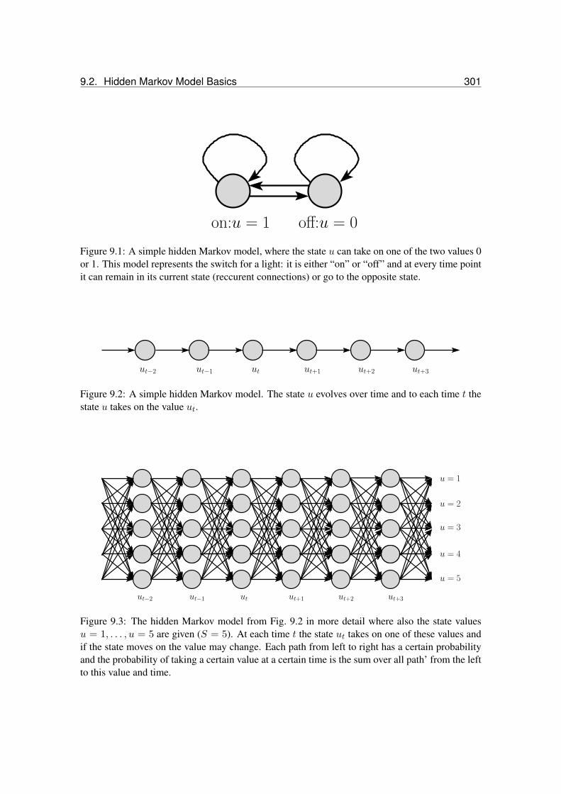
9.2. Hidden Markov Model Basics 301
on:u = 1 off:u = 0
Figure 9.1: A simple hidden Markov model, where the state u can take on one of the two values 0or 1. This model represents the switch for a light: it is either “on” or “off” and at every time pointit can remain in its current state (reccurent connections) or go to the opposite state.
ut−2 ut−1 ut ut+1 ut+2 ut+3
Figure 9.2: A simple hidden Markov model. The state u evolves over time and to each time t thestate u takes on the value ut.
ut−1 ut ut+1 ut+2 ut+3ut−2
u = 1
u = 2
u = 3
u = 4
u = 5
Figure 9.3: The hidden Markov model from Fig. 9.2 in more detail where also the state valuesu = 1, . . . , u = 5 are given (S = 5). At each time t the state ut takes on one of these values andif the state moves on the value may change. Each path from left to right has a certain probabilityand the probability of taking a certain value at a certain time is the sum over all path’ from the leftto this value and time.

302 Chapter 9. Hidden Markov Models
ut−2 ut−1 ut ut+1 ut+2 ut+3
Figure 9.4: A second order hidden Markov model. The transition probability does not dependonly on the current state value but also on the previous state value.
The hidden Markov model has transition probabilities p(a | b), where a, b ∈ 1, . . . , S andb is the current state and a the next state. Here the Markov assumption is that the next state onlydepends on the current state. Higher order hidden Markov models assume that the probability ofgoing into the next state depends on the current state and previous states. For example in a secondorder Markov model the transition probability is p(a | b, c), where a, b, c ∈ 1, . . . , S and b isthe current state, c the previous state, and a the next state. The second order Markov model isdepicted in Fig. 9.4.
We will focus on a first order hidden Markov model, where the probability of going into a statedepends only on the actual state.
At each time the state variable u takes on the value ut and has a previous value given byut−1, therefore we observed the transition from ut−1 to ut. This transition has probability ofp(ut | ut−1),
Assume we have a certain start state probability pS(u1) then the probability of observing thesequence uT = (u1, u2, u3, . . . , uT ) of length T is
p(uT ) = pS(u1)T∏t=2
p(ut | ut−1) . (9.1)
For example a sequence may be (u1 = 3, u2 = 5, u3 = 2, . . . , uT = 4) that is the sequence(3, 5, 2, . . . , 4). Fig. 9.5 shows the hidden Markov model from Fig. 9.3 where now the transitionprobabilities are marked including the start state probability pS .
Now we will consider Markov models which actually produce data, that means they are usedas generative models. We assume that each state value has an emission probability pE(xt | ut) ofemitting a certain output. Here ut is a value of the state variable at time t (e.g. ut = 2) and xt isan element of the output alphabet of size P , for example xt ∈ A, T,C,G. A specific emissionprobability may be pE(A | 2). Fig. 9.6 shows a hidden Markov model with output emission.
Fig. 9.7 shows a HMM where the output sequence is the Shine-Dalgarno pattern for ribosomebinding regions.
Each output sequence has a certain probability of being produced by the current model. Thejoint probability of the output sequence xT = (x1, x2, x3, . . . , xT ) of length T and the hiddenstate value sequence uT = (u1, u2, u3, . . . , uT ) of length T is
p(uT , xT ) = pS(u1)T∏t=2
p(ut | ut−1)T∏t=1
pE(xt | ut) . (9.2)

9.2. Hidden Markov Model Basics 303
Figure 9.5: The hidden Markov model from Fig. 9.3 where now the transition probabilities aremarked including the start state probability pS . Also the state value ut+1 = 4 is marked.
ut−2 ut−1 ut ut+1 ut+2 ut+3
xt−2 xt−1 xt xt+1 xt+2 xt+3
Figure 9.6: A simple hidden Markov model with output. At each time t the hidden state ut has acertain probability of producing the output xt.
G G A G G UA
Shine-Dalgarno pattern for ribosome binding
ut−2 = AG
ut−1 = AGG
ut = AGGA
ut+1 = AGGAG
ut+2 = AGGAGG
ut+3 = AGGAGGU
Figure 9.7: An HMM which supplies the Shine-Dalgarno pattern where the ribosome binds. Eachstate value is associated with a prefix sequence of the Shine-Dalgarno pattern. The state value for“no prefix” is omitted in the figure.

304 Chapter 9. Hidden Markov Models
Through marginalization we obtain the probability of the output sequence xT being producedby the HMM:
p(xT ) =∑uT
p(uT , xT ) =∑uT
pS(u1)T∏t=2
p(ut | ut−1)T∏t=1
pE(xt | ut) , (9.3)
where∑
uT denotes the sum over all possible sequences of length T of the values 1, . . . , S. Thesum
∑uT has ST summands corresponding to different sequences (S values for u1 multiplied by
S values for u2 etc.).
Fortunately, the (first order) Markov assumption allows to recursively compute above sum.We denote with xt = (x1, x2, x3, . . . , xt) the prefix sequence of xT of length t. We introduce theprobability p(xt, ut) of the model producing xt and being in state ut at the end.
p(xt, ut) = p(xt | xt−1, ut) p(xt−1, ut) = (9.4)
pE(xt | ut)∑ut−1
p(xt−1, ut, ut−1) =
pE(xt | ut)∑ut−1
p(ut | xt−1, ut−1) p(xt−1, ut−1) =
pE(xt | ut)∑ut−1
p(ut | ut−1) p(xt−1, ut−1) ,
where the Markov assumptions p(xt | xt−1, ut) = pE(xt | ut) on the output emission and p(ut |xt−1, ut−1) = p(ut | ut−1) and on the transitions is used. Further marginalization p(xt−1, ut) =∑
ut−1p(xt−1, ut, ut−1) and the definition of conditional probabilities p(xt−1, ut, ut−1) = p(ut |
xt−1, ut−1) p(xt−1, ut−1) was applied.
That means each recursion step needs only a sum over all ut−1 which is a sum over S val-ues. However we have to do this for each value of ut, therefore the recursion has complexity ofO(T S2). The complexity can be reduced if transition probabilities are zero. The recursion startswith
p(x1, u1) = pS(u1) pE(x1 | u1) . (9.5)
The final probability of xT can be computed as
p(xT ) =∑uT
p(xT , uT ) . (9.6)
This algorithm is called the “forward pass” or the “forward phase” and is used to compute theprobability of xT which is equal to the likelihood of xT because we have discrete values. Alg.9.1 shows the algorithm for the forward phase to compute the likelihood for one sequence for anHMM.

9.2. Hidden Markov Model Basics 305
Algorithm 9.1 HMM Forward Pass
Given: sequence xT = (x1, x2, x3, . . . , xT ), state values u ∈ 1, . . . , S, start probabilitiespS(u1), transition probabilities p(ut | ut−1), and emission probabilities pE(xt | ut); Output:likelihood p(xT ) and p(xt, ut)
BEGIN initialization
p(x1, u1) = pS(u1) pE(x1 | u1)END initializationBEGIN Recursion
for (t = 2 ; t ≤ T ; t+ +) dofor (a = 1 ; a ≤ S ; a+ +) do
p(xt, ut = a) = pE(xt | ut = a)S∑
ut−1=1
p(ut = a | ut−1) p(xt−1, ut−1)
end forend for
END RecursionBEGIN Compute Likelihood
p(xT ) =S∑a=1
p(xT , uT = a)
END Compute Likelihood

306 Chapter 9. Hidden Markov Models
9.3 Expectation Maximization for HMM: Baum-Welch Algorithm
Now we focus on learning and parameter selection based on a training set.
The parameters of a hidden Markov model are the S start probabilities pS(u1), the S2 transi-tions probabilities p(ut | ut−1), and the S P emission probabilities pE(xt | ut) (P is the numberof output symbols).
If we have a set of training sequences xi, 1 ≤ i ≤ l, then the parameter can be optimizedby maximizing the likelihood from Section 3.4.
Instead of gradient based methods from Chapter 5 we deduce a Expectation Maximizationalgorithm as shown in Subsection 3.4.6.
In Subsection 3.4.6 in eq. (3.77) we defined
F(Q,w) =∫UQ(u | x) ln p(x,u;w) du − (9.7)∫
UQ(u | x) lnQ(u | x) du ,
where Q(u | x) is an estimation for p(u | x;w).
We have to adapt this formulation to discrete HMMs. For HMMs u is the sequence of hid-den states, x the sequence of output states and w summarizes all probability parameters (start,transition, and emission) in the model. The integral
∫U du can be replaced by a sum.
The estimation for the state sequence can be written as
Q(u | x) = p(u1 = a1, u2 = a2, . . . , uT = aT | xT ;w) . (9.8)
We obtain
F(Q,w) =S∑
a1=1
. . .
S∑aT=1
(9.9)
p(u1 = a1, u2 = a2, . . . , uT = aT | xT ;w) ln p(xT , uT ;w) −S∑
a1=1
. . .
S∑aT=1
p(u1 = a1, u2 = a2, . . . , uT = aT | xT ;w)
ln p(u1 = a1, u2 = a2, . . . , uT = aT | xT ;w) = (9.10)S∑
a1=1
. . .
S∑aT=1
p(u1 = a1, u2 = a2, . . . , uT = aT | xT ;w) ln p(xT , uT ;w)
−c ,
where c is a constant independent of w.
We have
ln p(uT , xT ;w) = ln pS(u1) +T∑t=2
ln p(ut | ut−1) +T∑t=1
ln pE(xt | ut) . (9.11)

9.3. Expectation Maximization for HMM: Baum-Welch Algorithm 307
Because most variables at can be summed out we obtain:
F(Q,w) =S∑a=1
p(u1 = a | xT ;w) ln pS(u1 = a) + (9.12)
T∑t=1
S∑a=1
p(ut = a | xT ;w) ln pE(xt | ut = a) +
T∑t=2
S∑a=1
S∑b=1
p(ut = a, ut−1 = b | xT ;w) ln p(ut = a | ut−1 = b) − c .
Note that the parameters w are the start probabilities pS(a), the emission probabilities pE(x |a), and the transition probabilities p(a | b). We have as constraints
∑a pS(a) = 1,
∑x pE(x |
a) = 1, and∑
a p(a | b) = 1.
Consider the optimization problem
minw
∑t
∑a
cta lnwa (9.13)
s.t.∑a
wa = 1 .
The Lagrangian is
L =∑t
∑a
cta lnwa − λ
(∑a
wa − 1
). (9.14)
Optimality requires
∂L
∂wa=∑t
cta1wa− λ = 0 (9.15)
therefore∑t
cta − λ wa = 0 (9.16)
and summing over a gives∑a
∑t
cta = λ . (9.17)
We obtain
wa =∑
t cta∑a
∑t cta
. (9.18)

308 Chapter 9. Hidden Markov Models
The constraint maximization step (M-step) is therefore
pS(a) =p(u1 = a | xT ;w)∑a′ p(u1 = a′ | xT ;w)
(9.19)
pE(x | a) =∑T
t=1 δxt=x p(ut = a | xT ;w)∑y
∑Tt=1 δxt=y p(ut = a | xT ;w)
(9.20)
p(a | b) =∑T
t=2 p(ut = a, ut−1 = b | xT ;w)∑a′∑T
t=2 p(ut = a′, ut−1 = b | xT ;w)(9.21)
which is
pS(a) = p(u1 = a | xT ;w) (9.22)
pE(x | a) =∑T
t=1 δxt=x p(ut = a | xT ;w)∑Tt=1 p(ut = a | xT ;w)
(9.23)
p(a | b) =∑T
t=2 p(ut = a, ut−1 = b | xT ;w)∑Tt=2 p(ut−1 = b | xT ;w)
. (9.24)
We now consider the estimation step (E-step) in order to estimate p(ut = a | xT ;w) andp(ut = a, ut−1 = b | xT ;w). First we have to introduce the suffix sequence xt←T = (xt, xt+1, . . . , xT ).of length T − t+ 1.
We use the probability p(xt+1←T | ut = a) of the suffix sequence xt+1←T = (xt+1, . . . , xT )being produced by the model if starting from ut = a.
Now we can formulate an expression for p(ut = a | xT ;w)
p(ut = a | xT ;w) =p(ut = a, xT ;w)
p(xT )= (9.25)
p(xt, ut = a;w) p(xt+1←T | ut = a)p(xT )
,
where the first “=” is the definition of conditional probability and the second “=” say that all path’of hidden values with have at time t the value a can be separated into a prefix path from start totime t ending in the value a and a suffix path starting at time t in a.
Similar we can formulate an expression for p(ut = a, ut−1 = b | xT ;w)
p(ut = a, ut−1 = b | xT ;w) =p(ut = a, ut−1 = b, xT ;w)
p(xT )= (9.26)
p(xt−1, ut−1 = b;w) p(ut = a | ut−1 = b) pE(xt | ut = a)p(xt+1←T | ut = a) / p(xT ) ,
where again the first “=” is the conditional probability and the second “=” says all path’ which areat time t in state value a and in time (t− 1) in state value b can be separated in a prefix path fromstart to time (t − 1) ending in b, a suffix path starting from t in value a to the end, the transitionb← a with probability p(ut = a | ut−1 = b) and the emission of xt given by pE(xt | ut = a).

9.4. Viterby Algorithm 309
Note that
p(ut = a | xT ;w) =S∑b=1
p(ut = a, ut−1 = b | xT ;w) . (9.27)
Similar to eq. (9.4) we can derive a backward recursion for computing p(xt+1←T | ut = a) byusing the Markov assumptions:
p(xt+1←T | ut = a) = (9.28)S∑b=1
pE(xt+1 | ut+1 = b) p(ut+1 = b | ut = a) p(xt+2←T | ut+1 = b) .
The starting conditions are
p(xT←T | uT−1 = a) =S∑b=1
pE(xT | uT = b) p(uT = b | uT−1 = a) (9.29)
or, alternatively
∀a : p(xT+1←T | uT = a) = 1 (9.30)
In Alg. 9.2 an algorithm for the backward procedure for HMMs is given.
The EM algorithm for HMMs is given Alg. 9.3 which is based on the forward procedure Alg.9.1 and the backward procedure Alg. 9.2.
9.4 Viterby Algorithm
In the forward (and also backward) pass we computed p(xT ), the probability of producing xT bythe model, that is the likelihood of xT . The likelihood of xT is an integral – more exactly a sum –over all probabilities of possible sequences of hidden states multiplied by the probability that thehidden sequence emits xT .
In many cases a specific hidden sequence (uT )∗ = (u∗1, u∗2, u∗3, . . . , u∗T ) and its probability ofemitting xT dominates the above sum. More formally
(uT )∗ = arg maxuT
p(uT | xT ) = arg maxuT
p(uT , xT ) . (9.31)
(uT )∗ is of interest if the hidden states have a semantic meaning, then one want to extract(uT )∗.
In bioinformatics the extraction of (uT )∗ is important to make an alignment of a sequence witha multiple alignment stored in an HMM.

310 Chapter 9. Hidden Markov Models
Algorithm 9.2 HMM Backward Pass
Given: sequence xT = (x1, x2, x3, . . . , xT ), state values u ∈ 1, . . . , S, start probabilitiespS(u1), transition probabilities p(ut | ut−1), and emission probabilities pE(xt | ut); Output:likelihood p(xT ) and p(xt+1←T | ut = a)
BEGIN initialization
∀a : p(xT+1←T | uT = a) = 1END initializationBEGIN Recursion
for (t = T − 1 ; t ≥ 1 ; t−−) dofor (a = 1 ; a ≤ S ; a+ +) do
p(xt+1←T | ut = a) =S∑b=1
pE(xt+1 | ut+1 = b) p(ut+1 = b | ut = a) p(xt+2←T | ut+1 = b) .
end forend for
END RecursionBEGIN Compute Likelihood
p(xT ) =S∑a=1
pS(u1 = a) (p(x1←T | u1 = a)
END Compute Likelihood
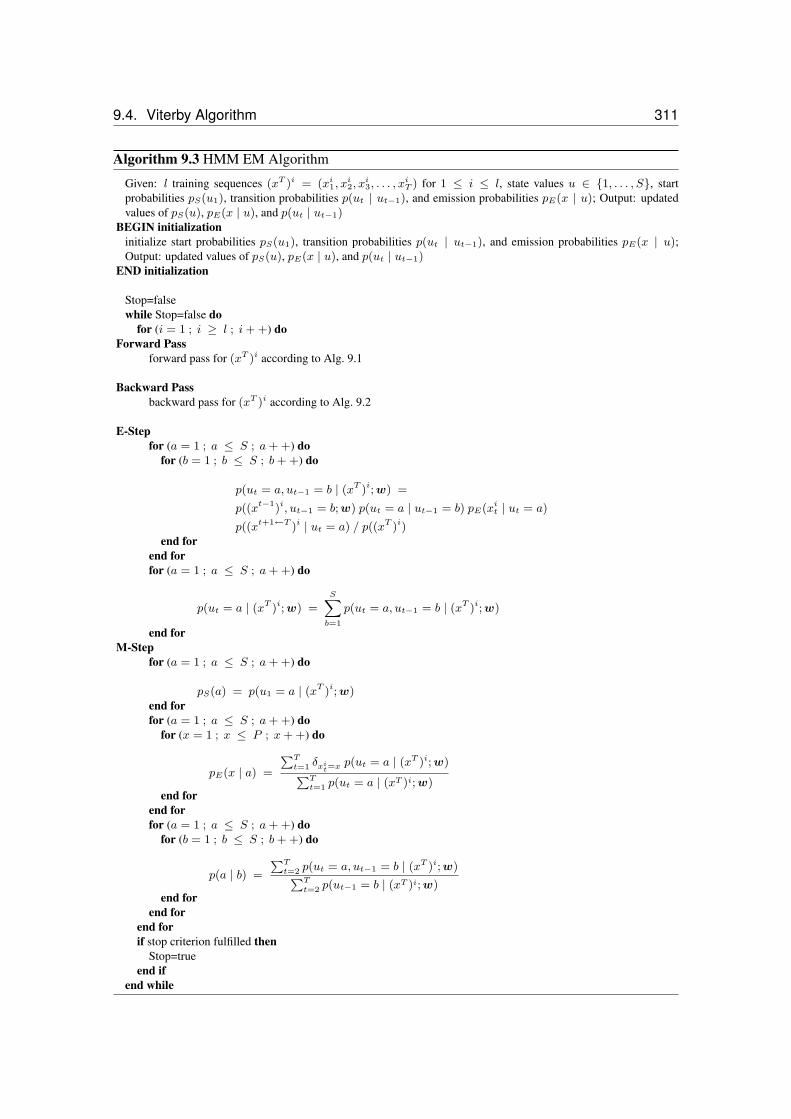
9.4. Viterby Algorithm 311
Algorithm 9.3 HMM EM Algorithm
Given: l training sequences (xT )i = (xi1, xi2, x
i3, . . . , x
iT ) for 1 ≤ i ≤ l, state values u ∈ 1, . . . , S, start
probabilities pS(u1), transition probabilities p(ut | ut−1), and emission probabilities pE(x | u); Output: updatedvalues of pS(u), pE(x | u), and p(ut | ut−1)
BEGIN initializationinitialize start probabilities pS(u1), transition probabilities p(ut | ut−1), and emission probabilities pE(x | u);Output: updated values of pS(u), pE(x | u), and p(ut | ut−1)
END initialization
Stop=falsewhile Stop=false do
for (i = 1 ; i ≥ l ; i+ +) doForward Pass
forward pass for (xT )i according to Alg. 9.1
Backward Passbackward pass for (xT )i according to Alg. 9.2
E-Stepfor (a = 1 ; a ≤ S ; a+ +) do
for (b = 1 ; b ≤ S ; b+ +) do
p(ut = a, ut−1 = b | (xT )i; w) =
p((xt−1)i, ut−1 = b; w) p(ut = a | ut−1 = b) pE(xit | ut = a)
p((xt+1←T )i | ut = a) / p((xT )i)end for
end forfor (a = 1 ; a ≤ S ; a+ +) do
p(ut = a | (xT )i; w) =
SXb=1
p(ut = a, ut−1 = b | (xT )i; w)
end forM-Step
for (a = 1 ; a ≤ S ; a+ +) do
pS(a) = p(u1 = a | (xT )i; w)end forfor (a = 1 ; a ≤ S ; a+ +) do
for (x = 1 ; x ≤ P ; x+ +) do
pE(x | a) =
PTt=1 δxi
t=x p(ut = a | (xT )i; w)PTt=1 p(ut = a | (xT )i; w)
end forend forfor (a = 1 ; a ≤ S ; a+ +) do
for (b = 1 ; b ≤ S ; b+ +) do
p(a | b) =
PTt=2 p(ut = a, ut−1 = b | (xT )i; w)PT
t=2 p(ut−1 = b | (xT )i; w)end for
end forend forif stop criterion fulfilled then
Stop=trueend if
end while

312 Chapter 9. Hidden Markov Models
Because (uT )∗ can be viewed as an alignment, it is not surprising that it can be obtainedthrough dynamic programming. The dynamic programming algorithm has to find a path in Fig.9.5 from left to right. Towards this end the state values at certain time which are the circles in Fig.9.5 are represented by a matrix V . Vt,a contains the maximal probability of a sequence of lengtht ending in state value a:
Vt,a = maxut−1
p(xt, ut−1, ut = a) . (9.32)
The Markov conditions allow now to formulate Vt,a recursively:
Vt,a = pE(xt | ut = a) maxbp(ut = a | ut−1 = b) Vt−1,b (9.33)
with initialization
V1,a = pS(a)pE(x1 | u1 = a) (9.34)
and the result
maxuT
p(uT , xT ) = maxa
VT,a . (9.35)
The best sequence of hidden states can be found by back-tracing using
b(t, a) = arg maxbp(ut = a | ut−1 = b) Vt−1,b (9.36)
The complexity of the Viterby algorithm is O(T S2) because all S T values Vt,a must becomputed and for computing them, the maximum over S terms must be determined.
The Viterby algorithm can be used to iteratively improve a multiple alignment:
1 initialize the HMM
2 align all sequences to the HMM via the Viterby algorithm
3 make frequency counts per column and compute the transition probabilities to update theHMM
4 if not converged go to step 2
9.5 Input Output Hidden Markov Models
Input Output Hidden Markov Models (IOHMMs) generates an output sequence xT = (x1, x2, x3, . . . , xT )of length T conditioned on an input sequence yT = (y1, y2, y3, . . . , yT ) of length T .
The difference between standard HMMs and input output HMMs is that the probabilities areconditioned on the input. Start probabilities are pS(u1 | y1), the transition probabilities p(ut |yt, ut−1), and the emission probabilities pE(xt | yt, ut).

9.5. Input Output Hidden Markov Models 313
Algorithm 9.4 HMM Viterby
Given: sequence xT = (x1, x2, x3, . . . , xT ), state values u ∈ 1, . . . , S, start probabilitiespS(u1), transition probabilities p(ut | ut−1), and emission probabilities pE(xt | ut); Output:most likely sequence of hidden state values (uT )∗ and its probability p
(xT , (uT )∗
)BEGIN initialization
V1,a = pS(a)pE(x1 | u1 = a)END initializationBEGIN Recursion
for (t = 2 ; t ≤ T ; t+ +) dofor (a = 1 ; a ≤ S ; a+ +) do
Vt,a = pE(xt | ut = a) maxbp(ut = a | ut−1 = b) Vt−1,b
b(t, a) = arg maxbp(ut = a | ut−1 = b) Vt−1,b
end forend for
END RecursionBEGIN Compute Probability
p(xT , (uT )∗
)=
Smaxa=1
V (T, a)
END Compute ProbabilityBEGIN Back-tracing
s = argS
maxa=1
V (T, a)
print sfor (t = T ; t ≥ 2 ; t−−) do
s = b(t, s)
print send for
END Back-tracing

314 Chapter 9. Hidden Markov Models
ut+2 ut+3ut−2 ut−1 ut ut+1
xt−2 xt xt+1 xt+2 xt+3
yt−2 yt−1 yt yt+1 yt+2 yt+3
xt−1
Figure 9.8: An input output HMM (IOHMM) where the output sequence xT =(x1, x2, x3, . . . , xT ) is conditioned on the input sequence yT = (y1, y2, y3, . . . , yT ).
Using IOMMs also negative examples can be used by setting for all yt either a don’t care or afixed value and setting yT = 1 for the positive class and yT = −1 for the negative class. Whethera model for the negative class can be build is not clear but at least a subclass of the negative classwhich is very similar to the positive class can be better discriminated.
The number of parameters increase proportional to the number of input symbols, which maymake it more difficult to estimate the probabilities if not enough data is available.
Learning via the likelihood is as with the standard HMM with the probabilities additionallyconditioned on the input.
9.6 Factorial Hidden Markov Models
The HMM architecture Fig. 9.6 is extended to Fig. 9.9 where the hidden state is divided into morecomponents ui (three in the figure).
The transition probability of ui is conditioned on all uk with k ≤ i and the emission probabilitydepends on all hidden states. The HMM architecture in Fig. 9.9 is meant that u1 evolves veryslowly, u2 evolves faster, and u3 evolves fastest of all hidden variables. Fast evolving variables donot influence slow evolving ones but slow evolving variables influence fast evolving variables.
If the factorial HMM has h hidden state variables ui and each one of them can take on S val-ues then the emission probability distribution consists of P Sh emission probabilities. Thereforelearning factorial HMMs is computational expensive. However approximative methods have beendeveloped to speed up learning [Ghahramani and Jordan, 1996, 1997].
9.7 Memory Input Output Factorial Hidden Markov Models
Remember that we quoted Sean Eddy [Eddy, 2004]:

9.7. Memory Input Output Factorial Hidden Markov Models 315
xt−2 xt xt+1 xt+2 xt+3xt−1
u3,t+2 u3,t+3u3,t−2 u3,t−1 u3,t u3,t+1
u2,t+2 u2,t+3u2,t−2 u2,t−1 u2,t u2,t+1
u1,t+2 u1,t+3u1,t−2 u1,t−1 u1,t u1,t+1
Figure 9.9: A factorial HMM with three hidden state variables u1, u2, and u3. The transitionprobability of ui is conditioned on all uk with k ≤ i and the emission probability depends on allhidden states.
“HMMs are reasonable models of linear sequence problems, but they don’t dealwell with correlations between residues or states, especially long-range correlations.HMMs assume that each residue depends only on one underlying state, and each statein the state path depends only on one previous state; otherwise, residues and states areindependent of each other.” ... “The state path of an HMM has no way of remember-ing what a distant state generated when a second state generates its residue.”
The only way a HMM can store information over time is to go into a certain state value anddon’t change it any more. The state is fixed and the event which led the HMM enter the fixed stateis memorized. Instead of a state a set of states can be entered from which the escape probability iszero.
To realize a state with a non-escaping value which can memorize past events is
p(ut = a | ut−1 = a) = 1 .
That means if the state takes on the value a then the state will not take any other value.
In principle the storage of past events can be learned but the likelihood of storing decreases ex-ponentially with the time of storage. Therefore learning to store is practically impossible becausethese small likelihood differences are tiny in comparison to local minima resulting from certaininput / output pattern or input / output distribution.
Therefore memory is enforced by setting p(ut = a | ut−1 = a) = 1 and to allowing thisprobability to change.
However after the storage process (taking on the value a) the model is fixed and neither futuresystems dynamics nor other events to memorize can be dealt with.
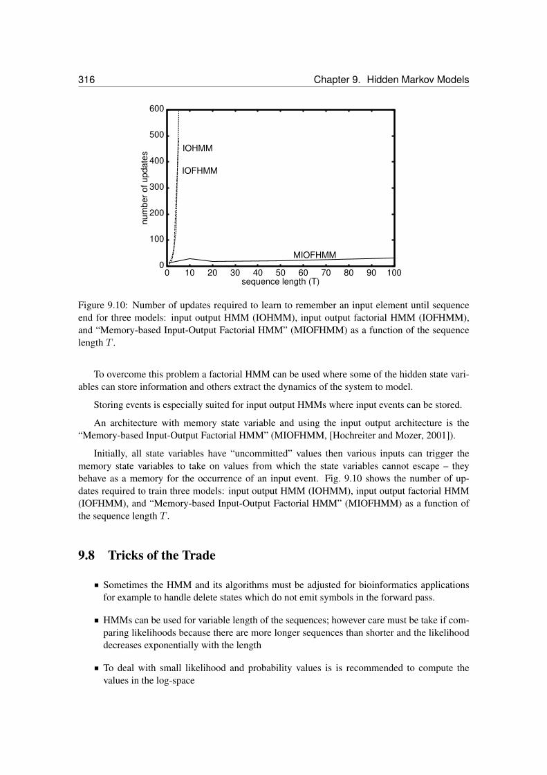
316 Chapter 9. Hidden Markov Models
0
100
200
300
400
500
600
0 10 20 30 40 50 60 70 80 90 100
num
ber o
f upd
ates
sequence length (T)
IOHMM
IOFHMM
MIOFHMM
Figure 9.10: Number of updates required to learn to remember an input element until sequenceend for three models: input output HMM (IOHMM), input output factorial HMM (IOFHMM),and “Memory-based Input-Output Factorial HMM” (MIOFHMM) as a function of the sequencelength T .
To overcome this problem a factorial HMM can be used where some of the hidden state vari-ables can store information and others extract the dynamics of the system to model.
Storing events is especially suited for input output HMMs where input events can be stored.
An architecture with memory state variable and using the input output architecture is the“Memory-based Input-Output Factorial HMM” (MIOFHMM, [Hochreiter and Mozer, 2001]).
Initially, all state variables have “uncommitted” values then various inputs can trigger thememory state variables to take on values from which the state variables cannot escape – theybehave as a memory for the occurrence of an input event. Fig. 9.10 shows the number of up-dates required to train three models: input output HMM (IOHMM), input output factorial HMM(IOFHMM), and “Memory-based Input-Output Factorial HMM” (MIOFHMM) as a function ofthe sequence length T .
9.8 Tricks of the Trade
Sometimes the HMM and its algorithms must be adjusted for bioinformatics applicationsfor example to handle delete states which do not emit symbols in the forward pass.
HMMs can be used for variable length of the sequences; however care must be take if com-paring likelihoods because there are more longer sequences than shorter and the likelihooddecreases exponentially with the length
To deal with small likelihood and probability values is is recommended to compute thevalues in the log-space

9.9. Profile Hidden Markov Models 317
To avoid zero probabilities for certain sequences which makes certain minima unreachableall probabilities can be kept above a threshold ε.
The EM-algorithm cannot reach probabilities which are exact zero, therefore, as an after-learning postprocessing all small probabilities ≤ ε can be set to zero. This often helps togeneralize from short to very long sequences.
HMM are prone to local minima, for example if HMMs are build from unaligned sequences.Global optimization strategies try to avoid theses minima, e.g. deterministic annealing wassuggested in the “Userguide” to HMMER version 1.8.
9.9 Profile Hidden Markov Models
Profile Hidden Markov Models code a multiple sequence alignment into a HMM as a position-specific scoring system which can be used to search databases for remote homologous sequences.Fig. 9.11 shows a HMM which can be used for homology search. The top row with states indicatedwith circles are a pattern. The diamond states are inserted strings. The bottom row with statesindicated as squares are deletions, where a letter from the pattern is skipped.
To learn an HMM from a set of unaligned positive examples suffers from the problem oflocal minima. Therefore expensive global optimization strategies must be used to avoid thesesminima, e.g. deterministic annealing was suggested in the “Userguide” to HMMER version 1.8.Therefore in most applications an HMM is at least initialized by a multiple alignment of thepositive examples.
The use of profile HMMs was made very convenient by the free HMMER package by SeanEddy [Eddy, 1998] which allows to to build and apply HMMs. HMMER supplies a log-oddslikelihood of the model compared to a random model to access the significance of the score ofa new sequence. Fig. 9.12 shows the architecture of the models used by HMMER. The statesindicated by squares and denoted by “Mx” are the consensus string. The circled states denoted by“Dx” are deletion states (non-emitting states), where part of the consensus string can be skipped.The diamond states denoted by “Ix” are insertion states where a substring can be inserted into theconsensus string
The other package which enabled a convenient use of HMMs for biological sequences isSequence Alignment and Modeling system (SAM – http://www.cse.ucsc.edu/research/
compbio/sam.html) which enables for creating, refining, and using HMMs for biological se-quence analysis. Also the SAM models represent a refinement of a multiple alignment. Modelscan be used to both generate multiple alignments and search databases for new members of thefamily.
Also databases like Protein FAMily database (Pfam) are based on HMMs. 67% of proteinscontain at least one Pfam profile HMM and 45% of residues in the protein database are covered intotal by the HMMs.
Another HMM application which is not associated with profile HMMs is shown in Fig. 9.13,where the HMM is used for splice site detection.

318 Chapter 9. Hidden Markov Models
Figure 9.11: Hidden Markov model for homology search. The top row with states indicated withcircles are a pattern. The diamond states are inserted strings. The bottom row with states indicatedas squares are deletions, where a letter from the pattern is skipped.
M1
S N B
M2 M3 M4
E C T
J
I1 I2 I3
D1 D2 D3 D4
Figure 9.12: The HMMER hidden Markov architecture. The states indicated by squares and de-noted by “Mx” form a pattern (consensus string). The circled states denoted by “Dx” are deletionstates (non-emitting), where a letter from the pattern can be skipped. The diamond states denotedby “Ix” are insertion states where a substring between letters of the pattern has been inserted. “B”and “E” denote the begin and end state of the pattern, respectively.

9.9. Profile Hidden Markov Models 319
Figure 9.13: An HMM for splice site detection.

320 Chapter 9. Hidden Markov Models

Chapter 10
Unsupervised Learning: ProjectionMethods and Clustering
10.1 Introduction
10.1.1 Unsupervised Learning in Bioinformatics
We have already seen an application of an unsupervised method in bioinformatics: the hiddenMarkov model. Hidden Markov models are used for sequence analysis.
One important topic in bioinformatics is to analyze microarray measurements with unsuper-vised techniques. Goals are to figure out which genes are expressed simultaneously (are part ofthe same pathway), what metabolic stages are present, etc. Also time series of microarray datamust be analyzed e.g. by cluster analysis (e.g. [Eisen et al., 1998]). Fig. 10.1 and Fig. 10.2 showmicroarray dendrograms obtained through hierarchical clustering.
Often unsupervised methods are used in bioinformatics to visualize dependencies and clusterslike the use of principal component analysis for Spellman’s cell-cycle data in Fig. 10.3.
For visualization the data must be in general down-projected to show the data in a 2-dimensionalor 3-dimensional space.
As we have already explained in Chapter 8 on feature selection, dimension reduction is an im-portant step in preprocessing biological data. In Chapter 8 we reported that with mass spectrometrythe data is huge and principal component analysis was used to reduce the input dimension. For ex-ample [Lilien et al., 2003] achieved best results on classification of healthy and cancerous personsof prostate Cancer on the basis surface-enhanced laser desorption/ionization time-of-flight massspectrometry (SELDI TOF MS) date if PCA was used.
10.1.2 Unsupervised Learning Categories
Many unsupervised learning procedures can be viewed as trying to bring two probability distribu-tions into alignment. Two well known classes of unsupervised procedures that can be cast in thismanner are generative and recoding models.
321

322 Chapter 10. Unsupervised Learning: Projection Methods and Clustering
Figure 10.1: A microarray dendrogram obtained by hierarchical clustering.
10.1.2.1 Generative Framework
In a generative unsupervised framework (see Fig. 10.4), the environment generates training exam-ples – which we will refer to as observations or training data – by sampling from one distribution;the other distribution is embodied in the model. In the generative framework we want to model orto simulate the real world by generating samples with the same underlying distribution as the realworld samples.
The hidden Markov models from previous Chapter 9 fall into the generative framework. Otherexamples of the generative framework are factor analysis [Jöreskog, 1967, Everitt, 1984, Nealand Dayan, 1997], Boltzmann machines [Hinton and Sejnowski, 1986], or mixture models. Inthe generative framework we have to bring two distributions to match: the fixed distribution ofobservations and the model output distribution.
10.1.2.2 Recoding Framework
In the recoding unsupervised framework (see Fig. 10.5), the model transforms observations to anoutput space. The distribution of the transformed observations (the outputs) is compared either to areference (target) distribution or whether target distribution features are present. These features aremeasured by an objective function which must be optimized. Target features are used to representa whole class of target distributions. In many cases the objective function can be replaced by thedistribution from the target distribution set which is closest to the output distribution.
Goal of the recoding framework is to represent the observations in an appropriate way, e.g.desired data density, low dimensional representation, high variance (large information), non-Gaussianity, or independent components.

10.1. Introduction 323
Figure 10.2: Another example of a microarray dendrogram obtained by hierarchical clustering.

324 Chapter 10. Unsupervised Learning: Projection Methods and Clustering
Figure 10.3: Spellman’s cell-cycle data represented through the first principal components (Land-grebe et al., Genome Biology, 2002).
world
modelsourcenoise
Figure 10.4: The generative framework is depicted. A noise source "drives" the model and pro-duces an output distribution which should match the distribution observed in the world. Separationof model and noise source means that all adjustable parameters are contained in the model.

10.1. Introduction 325
target
world
model
Figure 10.5: The recoding framework is depicted. The data from the world is mapped through amodel to a model output distributions which should match a specified target distribution.
Recoding Example: Density Estimation.Another special case of the recoding unsupervised framework is density estimation, where
the reference (target) distribution is easy to calculate like an uniform distribution or a Gaussiandistribution. A well known example is the mixtures of Gaussians (MoG) model [Pearson, 1894,Hasselblad, 1966, Duda and Hart, 1973]. The observation transformation must be locally invertiblethat is the Jacobian determinant must exists for the observation. That allows to compute the densityof the observation. Note that these constraints are weaker than assuming to know the inverse ofthe transformation. For example with neural networks the Jacobian can be computed [Flake andPearlmutter, 2000] and, therefore, it is local invertible but the inverse model is unknown.
Other Recoding Approaches.
Projection Pursuit and PCA. Other examples within the recoding framework are projectionmethods such as projection pursuit (e.g., [Friedman and Tukey, 1974, Friedman and Stuetzle,1981, Huber, 1985, Friedman, 1987, Jones, 1987, Jones and Sibson, 1987, Zhao and Atkeson,1996, Intrator, 1993]), principal component analysis (PCA) (e.g. [Oja, 1982, 1989, Jolliffe, 1986,Jackson, 1991]. Projection pursuit aims at an output distribution which is as non-Gaussian aspossible where the non-Gaussianity is measured by the entropy. Note, that for a given variance theGaussian distribution maximizes the entropy. PCA’s objective for an one-dimensional projectionis maximal variance. The projection is constraint to a linear mapping, the coefficient vector hasunit length, and is orthogonal to previous projections.
Clustering and Coincidence Detection. An objective function can be given for Clusteringmethods and Coincidence detection approaches. Clustering methods can be interpreted as mixturemodels and describe the data by a multimodal distribution. Coincidence detection is based onthe fact that the multidimensional distribution of observations has high density regions indicatingcorrelated components in the observations. Therefore coincidence detection is closely related toindependent component analysis.

326 Chapter 10. Unsupervised Learning: Projection Methods and Clustering
Self-organizing maps (SOMs). For self-organizing maps (SOMs) [Kohonen, 1982, 1988, 1990,1995, Ritter et al., 1992, 1991, Obermayer et al., 1992, Erwin et al., 1992] the objective function[cannot always be expressed as a single scalar function (like an energy or error function). Scalarobjectives are important to derive learning algorithms based on optimizing this function and tocompare models. The objective of SOMs is a scalar function for discrete input spaces and fordiscrete neighborhood functions otherwise the objective function must be expressed as a vectorvalued potential function [Kohonen, 1995, Cottrell et al., 1995, Ritter et al., 1992, 1991, Erwinet al., 1992]. The lack of a scalar objective function one of the major drawbacks of SOMs be-cause models cannot be compared, overfitting not detected, and stopping of training is difficult todetermine.
10.1.2.3 Recoding and Generative Framework Unified
If the recoding model has an unique inverse then the generative framework can be applied in therecoding context. The inverse model can use the observations as training examples which mustbe produced from some target distribution. Then the model maps the training examples to targetdistributions.
If the inverse model is obtained from the generative approach, then the recoding model is alsoavailable.
The objective function of principal component analysis (PCA) and independent componentanalysis (ICA) [Hinton and Sejnowski, 1999, Attias, 1999] attempt at keeping maximal informa-tion about the observations in the code while fulfilling certain constraints. In the generative viewthey are treated as generative models, which try to produce the data, whereas the constraints arecoded into the model e.g. by using specific target distributions.
However, most recoding methods have higher input dimensionality than output dimensionalitybecause the goal is to represent the input compactly and non-redundantly for visualization or forfeatures extraction.
However, it is sometimes possible to formulate the recoding approach as a generative modeleven for a non-bijective model. The target distribution has to produce the observations by firstgenerating a code which in turn generates the observations. Computing the likelihood requiredthe computations of the probabilities of the codes corresponding to the observations. Densityestimation, Projection pursuit and vector quantization can be treated is such a way [Hinton andSejnowski, 1999, Attias, 1999]. The probabilities of the codes are the posterior of the code giventhe data, where we assume that an observation can be produced by different codes. For exam-ple, recoding methods which do not have bijective functions are principal curves [Mulier andCherkassky, 1995, Ritter et al., 1992], which are a nonlinear generalization of principal compo-nents [Hastie and Stuetzle, 1989].
Example: Independent Component Analysis. An example for a recoding model treated as gen-erative model and using objective functions is independent component analysis (ICA) [Schmid-huber, 1992b, Bell and Sejnowski, 1995, Deco and Brauer, 1995, Pearlmutter and Parra, 1997,Cardoso and Laheld, 1996, Cichocki et al., 1994, Jutten and Herault, 1991, Comon, 1994, Yangand Amari, 1997, Yang et al., 1996, Cardoso and Souloumiac, 1993, Hyvärinen, 1999], a methodthat discovers a representation of vector-valued observations in which the statistical dependence

10.2. Principal Component Analysis 327
Figure 10.6: Principal component analysis for a two-dimensional data set. Left: the original dataset. Right: The first principal component is shown as the line from lower left to upper right. Thesecond principal component is orthogonal to the first component.
among the vector elements in the output space is minimized. With ICA, the model de-mixes ob-servation vectors and the output should consist of statistically independent components. Towardsthis end the output distribution can be compared against a given factorial distribution. The gen-erative approach assumes that the observations are produced by a model with independent hiddenunits [Cardoso, 1997, Moulines et al., 1997, Yang and Amari, 1997, Pearlmutter and Parra, 1997].Alternatively, an objective or contrast function indicating statistically independent model outputcomponents can be used (see e.g. [Hyvärinen, 1999]).
Example: Density Estimation. The traditional density estimation framework supplies the in-verse model and, therefore, can be viewed as a generative framework. For example in the mixtureof Gaussians model each mixture component can be viewed as being generated by a Gaussian dis-tribution with identity matrix as covariance matrix and thereafter transformed by a non-singularlinear mapping. The posterior can be easily computed thus the model can serve data generationmodel.
10.2 Principal Component Analysis
Principal Component Analysis (PCA) also known as Karhunen-Loève transform (KTL) or asHotelling transform makes a transformation of the coordinate system so that the first coordinatehas the largest variance of the data, the second largest data variance is on the second coordinate,etc. The coordinates are called principal components. Fig. 10.6 shows the principal componentsof a two-dimensional data set and Fig. 10.7 shows how the first principal component is extractedfrom some data points.
Let X =(x1, . . . ,xl
)T ∈ Rl×d be the matrix of data, then the data can be centered at theorigin by
X = X − 1l
1 1TX . (10.1)
Principal component analysis can be performed by computing the eigenvectors and eigenval-ues of the covariance matrix
C =1lXT X = WΛ2W T , (10.2)

328 Chapter 10. Unsupervised Learning: Projection Methods and Clustering
Figure 10.7: Principal component analysis for a two-dimensional data set. The first principalcomponent is extracted for some data points by projecting them onto the first component andmeasuring the distance to the origin.
where Λ is the diagonal matrix of the roots of the eigenvalues and W is the matrix of princi-pal components (the eigenvectors). The roots of the eigenvalues tell how much data variance isexplained by the corresponding eigenvector.
The projection
xTwi (10.3)
of a data vector x onto the i-th eigenvector wi is the i-th principal component of the data vectorx.
If we normalize the data so that
d∑i=1
λi = 1 (10.4)
and if the first k principal components are used to represent the data, then
E(MSE) =d∑
i=k+1
λi (10.5)
is the expected mean squared reconstruction error between the back-projected representation andthe original data.
Especially if the eigenvalues for the first principal components are large then most informationin the data can be represented by these first eigenvalues. This is important for down-projecting thedata for visualization.
The first principal component is described as
w1 = arg max‖w‖=1
E((wTx
)2)(10.6)
and the k-th as
wk = arg max‖w‖=1
E
(wT
(x −
k−1∑i=1
wi wTi x
))2 . (10.7)

10.3. Independent Component Analysis 329
Iterative methods for PCA are sometimes to prefer if the dimension d is large or if on-linemethods should be implemented.
Most famous is Oja’s rule [Oja, 1982]. First let us the projection define as
y = wTx . (10.8)
Oja’s rule is
wnew = w + η(y x − y2 w
), (10.9)
where η is the learning rate.
The eigenvectors of C are the fixed points of Oja’s rule and only the eigenvector with largesteigenvalue is a stable fixed point.
10.3 Independent Component Analysis
Independent Component Analysis (ICA) attempts at finding a code for the observation where thecomponents are mutually statistical independent.
The assumption for ICA is that the observations x are generated by mixing the sources s,where both x and s are d-dimensional vectors:
x = A s . (10.10)
Goal is to find a matrixW with
s = W x . (10.11)
The main assumption says that the sources are statistically independent:
p(s) =d∏j=1
p(sj) . (10.12)
Fig. 10.8 shows how two speaker (the sources s) speak independently from each other. Themicrophones record the acoustic signals and are the observations x.
In the optimal case we obtainW = A−1. However
x = A P P−1 s (10.13)
holds true for all permutation matrices P and all diagonal (scaling) matrices P . In this cases = P−1 s are sources which are statistically independent and can be mixed to give x withmixing matrixA P .
This means the problem formulation gives only unique solutions up to permutations and scal-ing.
Fig. 10.9 shows the ICA solution of the data set of Fig. 10.6 and Fig. 10.10 compares the PCAand the ICA solution.
Assumptions which must be made are

330 Chapter 10. Unsupervised Learning: Projection Methods and Clustering
Figure 10.8: Two speakers recorded by two microphones. The speakers produce independentacoustic signals which can be separated by ICA.
Figure 10.9: Independent component analysis on the data set of Fig. 10.6. Left subfigures showthe original data and the right subfigures the transformed data by ICA. The bottom line is the topline but the ICA components are shown.

10.3. Independent Component Analysis 331
Figure 10.10: Comparison of PCA and ICA on the data set of Fig. 10.6. Top: original data set.Bottom left: PCA solution. Bottom right: ICA solution.
the source components si are non-Gaussian (except for one component), because mixturesof Gaussians are Gaussians and no unique solution exists.
the observation dimension must be at least as large as the number of sources
the matrixA must have full rank.
We will combine the last two assumptions by assume that the observations x and the sources slive in a d-dimensional space andA−1 ∈ Rd×d exists.
If the densities p(si) are known or approximated – e.g. by super-Gaussians –, then the max-imum likelihood method can be applied. In this case the generative model is known and we canfirst estimateA and then computeW = A−1.
10.3.1 Measuring Independence
The entropy of a factorial code is larger than the entropy of the joint distribution. The differenceof the two expressions is the mutual information between the variables sj :
I(s1, . . . , sd) =d∑j=1
H(sj) − H(s) , (10.14)
where H denotes the entropy
H(a) = −∫p(a) ln p(a) da . (10.15)

332 Chapter 10. Unsupervised Learning: Projection Methods and Clustering
If we set
s = W x (10.16)
then
I(s1, . . . , sd) =d∑j=1
H(sj) − H(x) − ln |W | , (10.17)
where |W | is the absolute value of the determinant of the matrixW .
Above equation stems from the fact that
p(s) =p(x)|W | . (10.18)
The negentropy is defined as
J(y) = H(ygauss) − H(y) , (10.19)
where ygauss is a Gaussian random vector with the same covariance matrix as y. The negentropyis an affinely invariant version of the entropy.
The maximal negentropy is equivalent to representations where the mutual information be-tween the components is minimized. Here the connection between ICA and projection pursuit isclear because both can be expressed in maximize the distance to Gaussian distributions.
Unfortunately, the negentropy cannot be used easily because its estimation is difficult.
The non-Gaussianity can be measured through other parameters for example through the cum-mulants. For example the fourth cummulant, kurtosis is a common measure for non-Gaussianitywhere positive kurtosis indicates super-Gaussians (the tails are smaller than for Gaussians) andnegative kurtosis indicates sub-Gaussians (the tails are larger than for Gaussians).
For zero mean variables the cummulants are defined as
κ1 = E(x) = 0 (10.20)
κ2 = E(x2) (10.21)
κ3 = E(x3) (10.22)
κ4 = E(x4) − 3(E(x2)
)2. (10.23)
κ4 is called kurtosis. For Gaussians κ4 = 0 and for x1 and x2 independent:
κ4(x1 + x2) = κ4(x1) + κ4(x2) (10.24)
κ4(α x) = α4 κ4(x) . (10.25)
Many ICA algorithms use contrast functions which measure the independence of the variablesand are used as objective functions.
Common contrast functions are
10.3. Independent Component Analysis 333
κ4(y), the kurtosis
112 κ
23(y) + 1
48 κ24(y), where the variable y is normalized to zero mean and unit variance
|Ey(G(y)) − Eν(G(ν)))|p, where ν is a standardized Gaussian, p = 1, 2, and y is normal-ized to zero mean and unit variance. Here G can be the kurtosis for which G(ν) = 0 wouldhold. Other choices for G are G(x) = log cosh a x and G(x) = exp(−a x2/2) witha ≥ 1.
10.3.2 INFOMAX Algorithm
The INFOMAX algorithm is motivated by maximizing the entropy H(g(y)), where g is an acti-vation function of a neural network with output
g(yi) (10.26)
and
y = W x . (10.27)
If the entropy is maximized then
I(g(y1), . . . , g(yd)) =d∑j=1
H(g(yj)) − H(g(y)) = 0 (10.28)
and the components (g(y1), . . . , g(yd)) are statistically independent.
Very common choice for gi is
g(yi) = tanh(yi) . (10.29)
We have
p(g(y)) = p(x)∣∣∣∣∂g(y)∂y
∂y
∂x
∣∣∣∣−1
= p(x)∣∣∣∣∂g(y)∂y
W
∣∣∣∣−1
(10.30)
where ∣∣∣∣∂g(y)∂y
W
∣∣∣∣ =
∣∣∣∣∣∣d∏j=1
g′(yj)
∣∣∣∣∣∣ |W | . (10.31)
The entropy is then
H(g(y)) = E (− ln g(y)) = (10.32)
H(x) + E
d∑j=1
∣∣ln g′(yj)∣∣ + ln |W | ≈
H(x) +1l
l∑i=1
d∑j=1
∣∣ln g′(yij)∣∣ + ln |W | ,

334 Chapter 10. Unsupervised Learning: Projection Methods and Clustering
where
yi = W xi . (10.33)
Now we can maximize the entropy. Very common choice for gi is
g(yi) = tanh(yi) (10.34)
which gives
∂
∂wjln g′(yj) =
g′′(yj)g′(yj)
xT = − 2 g(yj) xT . (10.35)
For sigmoid activation function we have
∂
∂wjln g′(yj) = (1 − 2 g(yj)) xT . (10.36)
Further we have
∂
∂Wln |W | =
(W T
)−1. (10.37)
Because H(x) does not depend onW we obtain
∂
∂WH(g(y)) =
(W T
)−1 − 2 g(y) xT (10.38)
for tanh and for the sigmoid activation function
∂
∂WH(g(y)) =
(W T
)−1+ (1 − 2 g(y)) xT (10.39)
for the derivatives.
The update rules are for the tanh activation function
∆W ∝ (W T
)−1 − 2 g(y) xT (10.40)
and for the sigmoid activation function
∆W ∝ (W T
)−1+ (1 − 2 g(y)) xT . (10.41)
For this update rule the natural gradient can be applied which takes the geometrical structureof the parameter space into account. In this case the update rule is multiplied with W TW . Theupdate rule are now for the tanh activation function
∆W ∝ (I − 2 g(y) xT
)W (10.42)
and for the sigmoid activation function
∆W ∝ (I + (1 − 2 g(y)) xT
)W . (10.43)
INFOMAX is equivalent to a maximum likelihood approach, when g′i(si) = p(si).

10.4. Factor Analysis 335
10.3.3 EASI Algorithm
The EASI algorithm uses the following update rule:
∆W ∝ (I − y yT − g(y)yT + y gT (y)
)W . (10.44)
Here the nonlinear functions g are similar to the functions used by INFOMAX.
10.3.4 FastICA Algorithm
The FastICA algorithm is an fixed point algorithm which was originally based on the kurtosis andextracts a weight vector w.
The iteration step of the FastICA algorithm is
wnew = E(x g(wT x)
) − E(g′(wT x)
)w , (10.45)
where g is the derivative of the contrast function, which has been defined above.
Instead of the expectation E the empirical mean over the training examples is used.
10.4 Factor Analysis
Here we focus on the maximum likelihood factor analysis. In contrast to PCA, factor analysishas the advantage that it is a generative approach and it does model the independent noise at theobservations. Disadvantage of factor analysis is that it has to make assumptions on the distributionlike that the factors are Gaussian and the noise is Gaussian.
We are given the data x = x1, . . . ,xl which is already normalized to mean zero (bysubtracting the mean µ from the data). The model is
x = Λz + ε , (10.46)
where
z ∼ N (0, I) and ε ∼ N (0,Ψ) . (10.47)
The observations x, ε ∈ Rd, the factors z ∈ Rp, the factor loading matrix Λ ∈ Rd×p, and thenoise covariance matrix Ψ is a diagonal matrix from Rd×d.
In general the model has fewer factors than observations: d ≥ p. The diagonal form of Ψis reasonable if the measurements are taken independently and the noise at the components aremutually independent. Therefore, the observations are mutually independent if the factors areknown (only the noise is the random component).
Correlations between observations can only be explained by factors.
We assume that ε and z are independent which must not be true for all systems, e.g. if thenoise changes with the signal strength.

336 Chapter 10. Unsupervised Learning: Projection Methods and Clustering
noise ε
z2
x1 x2 x3 x4
z1
λ42
λ22
ε2 ε3 ε4ε1
factor z
observations x
loading matrix Λ
Figure 10.11: The factor analysis model.
The free parameters of the model are Λ and Ψ, which can be estimated by maximum like-lihood. Both parameter sets explain the variance in the observations x, however Λ explains thedependent part whereas Ψ explains the independent part of the variance. The factors are compara-ble with the principal components of the PCA method and data components can be projected ontothem.
Fig. 10.11 depicts the factor analysis model.
We have
x | z ∼ N (Λz,Ψ) , (10.48)
because if z is given, then only the noise distribution is present.
We focus on the maximum likelihood approach to factor analysis is in most cases [Jöreskog,1967] based on the Expectation-Maximization (EM) optimization technique [Dempster et al.,1977].
We will now consider the likelihood of the data. Let denote E the expectation of the data(i.e. the factor distribution and the noise distribution is combined), then we obtan for the first twomoments:
E(x) = E(Λz + ε) = ΛE(z) + E(ε) = 0 , (10.49)
E(x xT
)= E
((Λz + ε)(Λz + ε)T
)=
ΛE(z zT
)ΛT + ΛE (z) E
(εT)
+ E (z) E (ε) ΛT + E(ε εT
)=
Λ ΛT + Ψ .
The variance can be computed as
var(x) = E(x xT
) − (E(x))2 = (10.50)
Λ ΛT + Ψ .
Therefore, the marginal distribution for x is
x ∼ N (0 , ΛΛT + Ψ). (10.51)

10.4. Factor Analysis 337
This means that the observations are Gaussian distributed. This is an assumption of the factoranalysis model which can be checked to see whether the model is applicable to a certain problem.
The log-likelihood of the data x under the model (Λ,Ψ) is
logl∏
i=1
(2π)−d/2∣∣ΛΛT + Ψ
∣∣−1/2(10.52)
exp(−1
2
((xi)T
(ΛΛT + Ψ
)−1xi))
,
where |.| denotes the absolute value of the determinant of a matrix.
To maximize the likelihood is difficult because no closed form of directly maximizing thelikelihood with respect to the parameters is known.
We again apply the EM-algorithm. We introduce a distribution which estimates the hiddenstates, here the factors.
Using
Qi(zi) = p(zi | xi; Λ,Ψ) (10.53)
then
zi | xi ∼ N (µzi|xi ,Σzi|xi)
(10.54)
µzi|xi =(xi)T (
Λ ΛT + Ψ)−1
Λ
Σzi|xi = I − ΛT(Λ ΛT + Ψ
)−1Λ +(
Λ ΛT + Ψ)−1
xi (xi)T(Λ ΛT + Ψ
)−1,
where we used the fact that
v ∼ N (µv,Σvv) , u ∼ N (µu,Σuu) , (10.55)
Σuv = Covar(u,v) and Σvu = Covar(v,u) :v | u ∼ N (µv + ΣvuΣ−1
uu (u − µu) , Σvv + ΣvuΣ−1uuΣuv
)and
E(zx) = Λ E(z zT ) = Λ . (10.56)
We obtain
Qi(zi) = (2π)−d/2∣∣Σzi|xi
∣∣−1/2 (10.57)
exp(−1
2(zi − µzi|xi
)TΣ−1zi|xi
(zi − µzi|xi
)).
338 Chapter 10. Unsupervised Learning: Projection Methods and Clustering
The EM algorithm for maximum likelihood maximizes in the M-step a lower bound for thelikelihood:
log(p(xi | Λ,Ψ)
)= (10.58)
log(∫
Rp
Qi(zi) p(xi, zi | Λ,Ψ)Qi(zi)
dzi)≥∫
RpQi(zi) log
(p(xi, zi | Λ,Ψ)
Qi(zi)
)dzi .
Using the expectation
Ezi|xi(f(zi)
)=∫
RpQi(zi) f(zi) dzi (10.59)
and neglecting all terms which are independent of Λ and Ψ, the M-step requires to maximize
logL =d l
2log (2π) − l
2log |Ψ| − (10.60)
12
l∑i=1
Ezi|xi((xi − Λzi
)TΨ−1
(xi − Λzi
)).
The optimality criteria are
1l∇Λ logL =
1l
l∑i=1
Ψ−1 Λ Ezi|xi(zi (zi)T
) −1l
l∑i=1
Ψ−1 xi Ezi|xi(zi)
= 0 (10.61)
and
∇Ψ logL = − l2Ψ−1 + (10.62)
12
l∑i=1
Ezi|xi(Ψ−1
(xi − Λzi
) (xi − Λzi
)TΨ−1
)= 0 .
Solving above equations gives:
Λnew =
(1l
l∑i=1
xi Ezi|xi(zi)) (
1l
l∑i=1
Ezi|xi(zi (zi)T
))−1
(10.63)

10.4. Factor Analysis 339
and
Ψnew = (10.64)
diag
(1l
l∑i=1
Ezi|xi((xi − Λnewzi
) (xi − Λnewzi
)T)) =
diag
(1l
l∑i=1
xi (xi)T − 1l
l∑i=1
Ezi|xi(zi)xi (Λnew)T −
1l
l∑i=1
Ezi|xi(zi)Λnew(xi)T +
1l
l∑i=1
Ezi|xi(zi (zi)T
)Λnew (Λnew)T
),
where “diag” makes a diagonal matrix from a matrix by setting all non-diagonal elements to zero.
From eq. (10.63) we obtain
Λnew
(1l
l∑i=1
Ezi|xi(zi (zi)T
))=
(1l
l∑i=1
xi Ezi|xi(zi))
. (10.65)
and can replace the left hand side of above equation in the last term of eq. (10.64) which leads tothe fact that one term 1
l
∑li=1 Ezi|xi
(zi)Λnew(xi)T cancels in eq. (10.64). We obtain
Ψnew =1ldiag
(l∑
i=1
xi (xi)T −l∑
i=1
Ezi|xi(zi)xi (Λnew)T
). (10.66)
This leads to following EM updates:
E-step: (10.67)
Ezi|xi(zi)
= µzi|xi
Ezi|xi(zi (zi)T
)= µzi|xi µ
Tzi|xi + Σzi|xi
M-step: (10.68)
Λnew =(1l
l∑i=1
xi Ezi|xi(zi)) (
1l
l∑i=1
Ezi|xi(zi (zi)T
))−1
Ψnew = (10.69)
1ldiag
(l∑
i=1
xi (xi)T −l∑
i=1
Ezi|xi(zi)xi (Λnew)T
).

340 Chapter 10. Unsupervised Learning: Projection Methods and Clustering
Speed Ups. To speed up the algorithm for especially for d > p the matrix inversion lemmacan be used:
(Λ ΛT + Ψ
)−1= Ψ−1 − Ψ−1Λ
(I + ΛTΨ−1Λ
)−1ΛTΨ−1 , (10.70)
where Ψ−1 can be evaluated very fast because it is a diagonal matrix.
Another speed up is obtained
1l
l∑i=1
xi Ezi|xi(zi)
= (10.71)(1l
l∑i=1
xi(xi)T ) (
Λ ΛT + Ψ)−1
Λ =
C(Λ ΛT + Ψ
)−1Λ =
C(Ψ−1Λ − Ψ−1Λ
(I + ΛTΨ−1Λ
)−1ΛTΨ−1Λ
)=
C(A − A (I + B)−1B
),
where A = Ψ−1Λ, B = ΛTΨ−1Λ = ΛTA, and C is the empirical covariance matrix, whichhas to be computed only once.
We can also compute
1l
l∑i=1
Σzi|xi = (10.72)
I − ΛT(Λ ΛT + Ψ
)−1Λ +(
Λ ΛT + Ψ)−1
(1l
l∑i=1
xi (xi)T)(
Λ ΛT + Ψ)−1
=
I − ΛT Ψ−1Λ + ΛT Ψ−1Λ(I + ΛTΨ−1Λ
)−1ΛTΨ−1Λ +(
Ψ−1 − Ψ−1Λ(I + ΛTΨ−1Λ
)−1ΛTΨ−1
)C(
Ψ−1 − Ψ−1Λ(I + ΛTΨ−1Λ
)−1ΛTΨ−1
)=
I − B + B (I + B)−1B +(Ψ−1 − A (I + B)−1AT
)C(Ψ−1 − A (I + B)−1AT
)

10.4. Factor Analysis 341
and
1l
l∑i=1
µzi|xi µTzi|xi = (10.73)
ΛT(Λ ΛT + Ψ
)−1
(1l
l∑i=1
xi(xi)T) (
Λ ΛT + Ψ)−1
Λ =
ΛT(Λ ΛT + Ψ
)−1C(Λ ΛT + Ψ
)−1Λ =(
A − A (I + B)−1B)TC(A − A (I + B)−1B
).
Using these equations the E-step and the M-step can be unified and all sums∑l
i=1 are removedand the matrix C can be computed once at the beginning of the iterative procedure.
MAP factor analysis. This algorithm can be generalized to a maximum a posteriori methodwith posterior p(Λ,Ψ | x) which is proportional to the product between the likelihood p(x |Λ,Ψ) and the prior p(Λ):
p(Λ,Ψ | x) ∝ p(x | Λ,Ψ) p(Λ) , (10.74)
therefore up to a constant independent of the parameters the log-posterior is
log (p(Λ,Ψ | x)) = log (p(x | Λ,Ψ)) + log (p(Λ)) . (10.75)
An example for the prior on λj is a rectified Gaussian Nrect (µΛ, σΛ) in order to allow onlypositive factor loading values which assume that the factors are only additive:
yj ∼ N (µΛ, σΛ) (10.76)
λj = maxyj , 0 . (10.77)
MAP factors. The E-step gives also the most probable values for the factors z. This can beimportant for analyzing data and extracting hidden causes.
Interpretation. We already mentioned that the data variance is explained through signal vari-ance and through noise. The communality cj of an observations variable xj is
cj =var(xj) − var(εj)
var(xj)=
Ψjj
Ψjj +∑p
k=1 λ2jk
(10.78)
which is the proportion in xi explained by the factors. Here each factor zl contributes
λ2jl
Ψjj +∑p
k=1 λ2jk
. (10.79)

342 Chapter 10. Unsupervised Learning: Projection Methods and Clustering
10.5 Projection Pursuit and Multidimensional Scaling
10.5.1 Projection Pursuit
Projection pursuit attempts to find “interesting” projections of the data in order to visualize, clusterthe data or for dimensionality reduction.
“Interesting” is defined as the least Gaussian distribution. The important question is how todefine non-Gaussianity.
If the covariance of a zero mean variable y is fixed, then a Gaussian distribution maximizesthe entropy H(y).
Then for y = wTx the vectorw must be found which maximized H(y) if y is normalized tozero mean and unit variance.
However the density of y = wTx is difficult to estimate.
Other more practical measures of non-Gaussianity have been given in as independent compo-nent analysis was introduced in Subsection 10.3.1.
10.5.2 Multidimensional Scaling
Multidimensional Scaling (MDS) aims at representing data points x by y in a lower dimensionalspace so that he distances between the y’s correspond to the distances (dissimilarities) betweenthe x’es.
We define
yi = f(xi;w) (10.80)
δij =∥∥xi − xj
∥∥ (10.81)
dij =∥∥yi − yj
∥∥ . (10.82)
The goal is to define a measure which measures the difference between δ and d which is mostlydone by a weighted sum of the differences between δij and dij .
Possible measures are
R1(d, δ) =
∑i<j (dij − δij)
2∑i<j δ
2ij
∝∑i<j
(dij − δij)2 (10.83)
R2(d, δ) =∑i<j
(dij − δij
δij
)2
(10.84)
R3(d, δ) =1∑i<j δij
∑i<j
(dij − δij)2
δij∝∑i<j
(dij − δij)2
δij, (10.85)
where “∝” removed factors which are constant in the parameters w.
The measure R1 is basically the mean squared error and penalizes large errors even if theδij are large. The measure R2 measures the fractional errors (relative errors) but small δij mayincrease the relative error. R3 is called “Sammon mapping” and is an compromise of R1 and R2.

10.6. Clustering 343
x1
x2
x3
xi xj
δij
s o u r c e s p a c e ta r g e t s p a c e
y1
y2
yi
yj
dij
s o u r c e s p a c e ta r g e t s p a c e
Figure 10.12: Example for multidimensional scaling. Points x from a 3-dimensional space (left)are mapped by multidimensional scaling to a 2-dimensional space (right). Copyright c© 2001 JohnWiley & Sons, Inc.
The derivatives which can be used in gradient based methods are
∂
∂ykR1(d, δ) =
2∑i<j δ
2ij
∑j 6=k
(dkj − δkj)yk − yjdkj
(10.86)
∂
∂ykR2(d, δ) = 2
∑j 6=k
dkj − δkjδ2kj
yk − yjdkj
(10.87)
∂
∂ykR3(d, δ) =
2∑i<j δij
∑j 6=k
dkj − δkjδkj
yk − yjdkj
. (10.88)
If the measures are viewed as potential functions, then the derivatives can be considered asforces on certain points yk.
Fig. 10.12 shows and example for multidimensional scaling.
10.6 Clustering
One of the most popular unsupervised learning techniques is clustering. Here “clusters” in thedata, that is regions of high data density, are identified. Often these clusters represent typically datapoints which stem from one “prototype data point” by noise perturbations or represent a certainsituation in the real world where the situation is expressed as dependencies in the components.
Clustering extracts structure in the data. Often clustering identifies new data classes whichwere unknown so far.

344 Chapter 10. Unsupervised Learning: Projection Methods and Clustering
An important application of clustering is also data visualization where is some cases bothdown-projection and clustering are combined (e.g. for self-organizing maps).
If data points are represented by their prototypes then clustering is a data compression methodcalled “vector quantization”.
10.6.1 Mixture Models
Because clusters are regions of high data density, density estimators which locally assign a com-ponent can be used for clustering. A local component j out of c components has a location µj , awidth or shape Σj and a weight wj giving the local probability mass.
If we consider this as a generative model, then wj is the probability p(j) of choosing compo-nent j. The values µj and Σj describe the local component j which has density p(x | j,µj ,Σj).
If we summarize all parameters µj , Σj , and w in the parameter vector θ, then we obtain themodel
p(x | θ) =c∑j=1
p(j) p(x | j,µj ,Σj) . (10.89)
The log-likelihood is
lnL =l∑
i=1
ln p(xi | θ) . (10.90)
If we summarize µj and Σj in θj then the derivative of the log-likelihood is
∂
∂θjlnL =
l∑i=1
1p(xi | θ)
c∑j=1
p(j)∂
∂θjp(xi | j,µj ,Σj) = (10.91)
l∑i=1
p(j | xi,µj ,Σj)∂
∂θjln p(xi | j,µj ,Σj) ,
where we used Bayes’ formula
p(j | xi,µj ,Σj) =p(xi | j,µj ,Σj) p(j)
p(xi | θ). (10.92)
The derivative of the log-likelihood of the model with respect to the parameters of the j com-ponent is posterior expectation of component j of the derivative of the log-likelihood of the com-ponent j.
These consideration are valid of each mixture model.
We will now consider mixture of Gaussian (MoG), where
p(xi | j,µj ,Σj) ∼ N (µj , Σj) . (10.93)

10.6. Clustering 345
The model is
p(x | θ) =c∑j=1
wj N (µj , Σj) (10.94)
c∑j=1
wj = 1 (10.95)
wj ≥ 0 (10.96)
N (µj , Σj) (x) = (10.97)
(2π)−d/2 |Σj |−1/2 exp(−1
2(x − µj)
T Σ−1j (x − µj)
).
Gaussian are convenient because in eq. (10.91) the logarithm inverts the exponential function:
ln p(x | j,µj ,Σj) = (10.98)
− d
2ln (2π) − 1
2ln |Σj | − 1
2(x − µj)
T Σ−1j (x − µj)
which gives for the derivatives
∂
∂µjln p(x | j,µj ,Σj) = Σ−1
j (x − µj) (10.99)
∂
∂Σjln p(x | j,µj ,Σj) = (10.100)
12(ΣTj
)−1+
12
Σ−Tj (x − µj) (x − µj)T Σ−Tj .
Here also the EM-algorithm can be used where the hidden parameters are p(j | xi,µj ,Σj)must be estimated to evaluate eq. (10.91).
The EM-algorithm is
E-step: (10.101)
p(j | xi,µj ,Σj) =wj N (µj , Σj) (xi)∑cl=1wl N (µl , Σl) (xi)
M-step: (10.102)
wnewj =
1l
l∑i=1
p(j | xi,µj ,Σj)
µnewj =
∑li=1 p(j | xi,µj ,Σj) xi∑li=1 p(j | xi,µj ,Σj)
(10.103)
Σnewj =
∑li=1 p(j | xi,µj ,Σj)
(xi − µj
) (xi − µj
)T∑li=1 p(j | xi,µj ,Σj)
. (10.104)

346 Chapter 10. Unsupervised Learning: Projection Methods and Clustering
In order to avoid too small variances and near zero eigenvalues of Σj the mixture of Gaussiancan be optimized by a maximum a posterior approach.
A proper prior for the covariance Σ is the Wishart densityW(Σ−1 | α,Ψ), a proper prior forthe weighting factors wj is a Dirichlet density D(w | γ), and a proper prior for the mean values µis a Gaussian N (µ | ν, η−1Σ
):
W(Σ−1 | α,Ψ) = c(α,Ψ)∣∣Σ−1
∣∣α−(d+1)/2 exp(−tr
(Ψ Σ−1
))(10.105)
D(w | γ) = c(γ)c∏j=1
wγ−1j (10.106)
N (µ | ν, η−1Σ)
= (10.107)
(2π)−d/2∣∣η−1 Σj
∣∣−1/2 exp(−η
2(µ − ν)T Σ−1
j (µ − ν)),
where α > (d− 1)/2 and c(γ) as well as c(α,Ψ) are normalizing constants. The operator “tr” isthe trace operator.
The expectation-maximization algorithm is now
E-step: (10.108)
p(j | xi,µj ,Σj) =wj N (µj , Σj) (xi)∑cl=1wl N (µl , Σl) (xi)
M-step: (10.109)
wnewj =
∑li=1 p(j | xi,µj ,Σj) + γ − 1
l + c (γ − 1)
µnewj =
∑li=1 p(j | xi,µj ,Σj) xi + η νj∑l
i=1 p(j | xi,µj ,Σj) + η(10.110)
Σnewj =
(l∑
i=1
p(j | xi,µj ,Σj)(xi − µj
) (xi − µj
)T + (10.111)
η (νj − µj) (νj − µj)T + 2 Ψ
)(
l∑i=1
p(j | xi,µj ,Σj) + 2 α − d)−1
.
Above formulae are obtained as follows: Because
c∑j=1
wnewj = 1 (10.112)

10.6. Clustering 347
we obtain as Lagrangian for the constraint optimization problem for the wj
L =l∑
i=1
c∑j=1
p(j | xi,µj ,Σj) lnwnewj + lnD(w | γ) − (10.113)
λ
c∑j=1
wnewj − 1
.
Setting the derivative to zero:
∂L
∂wj=
l∑i=1
p(j | xi,µj ,Σj)(wnewj
)−1 + (10.114)
(γ − 1)(wnewj
)−1 − λ = 0l∑
i=1
p(j | xi,µj ,Σj) + (γ − 1) = λ wnewj
Summing over j gives
l∑i=1
c∑j=1
p(j | xi,µj ,Σj) + c (γ − 1) = λc∑j=1
wnewj (10.115)
l + c (γ − 1) = λ (10.116)
We obtain
wnewj =
∑li=1 p(j | xi,µj ,Σj) + (γ − 1)
l + c (γ − 1)(10.117)
For the other parameters we do not have constraints. The gradient of the log-posterior LP withrespect to µj contains the log-likelihood and the log-prior:
∂LP∂µj
=l∑
i=1
p(j | xi,µj ,Σj) Σ−1j
(xi − µj
)+ (10.118)
η Σ−1j (νj − µj) = 0 .
For the gradient with respect to Σj a trick is applied: the gradient is taken with respect to Σ−1j
with also must be zero at the minimum, because
∂LP∂Σj
= − Σ−2j
∂LP∂Σ−1
j
(10.119)
and the variables Σ−1j fully represent the variables Σj .

348 Chapter 10. Unsupervised Learning: Projection Methods and Clustering
We obtain
∂LP∂Σ−1
j
= (10.120)
12
l∑i=1
p(j | xi,µj ,Σj)(Σj −
(xi − µj
) (xi − µj
)T) +
12
(Σj − η (νj − µj) (νj − µj)
T)
+
Σj (α − (d + 1)/2) − Ψ = 0 ,
where we used
∂ ln |A|∂A
= A−1 (10.121)
forA = Σ−1j .
Note that each component can have prior so that we would obtain νj , ηj , αj , Ψj , and γj . Theupdate formulae would we similar as above.
Default values for the hyperparameters are
α =d
2(10.122)
Ψ =12I OR Ψ =
12
covar(x) (10.123)
γ = 1 (10.124)
η = 0 (10.125)
νj = mean(x) (10.126)
A prior on the mean values µ is in most cases not useful except a preferred region is known.
The posterior p(j | xi,µj ,Σj) can be used for clustering: xi belongs to the cluster j forwhich the posterior is largest.
But also soft clustering is possible: p(j | xi,µj ,Σj) gives the graded or fuzzy membership ofxi to the cluster j.
10.6.2 k-Means Clustering
p(j | xi,µj ,Σj) in eq. (10.101) is determined by the weight wj of the jth component and thedistance
(xi − µj
)T Σ−1j
(xi − µj
)of xi to the mean µj .
If we set wj = 1c and Σ−1
j = I , then xi belongs to the cluster j which center µj has thesmallest Euclidean distance
∥∥xi − µj∥∥ to xi.
If we discretize
p(j | xi,µj) =
1 if j = cxi = arg minl∥∥xi − µl
∥∥0 otherwise
(10.127)

10.6. Clustering 349
then the M-step in eq. (10.102) is
µnewj =
1lj
l∑i=1, j=cxi
xi (10.128)
lj =l∑
i=1
p(j | xi,µj ,Σj) =l∑
i=1, j=cxi
1 , (10.129)
where lj is the number of data points assigned to cluster j.
Therefore µnewj is the mean of the data points assigned to cluster j. This method is called
k-means clustering and its algorithm is given in Alg. 10.1.
Algorithm 10.1 k-means
Given: data x = (x1,x2, . . . ,xl), number of clusters c
BEGIN initializationinitialize the cluster centers µj , 1 ≤ j ≤ c
END initialization
BEGIN Iteration
Stop=falsewhile Stop=false do
for (i = 1 ; i ≥ l ; i+ +) doassign xi to the nearest µj
end forfor (j = 1 ; j ≥ c ; j + +) do
µnewj =
1lj
l∑i=1, j=cxi
xi
end forif stop criterion fulfilled then
Stop=trueend if
end whileEND Iteration
The k-means clustering is fast but it is prone to initial initialization. For example consider aninitialization which places one center near an outlier data point which is separated from the restof the data points which all have other cluster centers closer to them. Then this outlier cluster willcontain in each iteration only one data point.
This behavior can be serious in high dimensions.
Let us again assume wj = 1c and Σ−1
j = I . But now we use a continuous estimate ofp(j | xi,µj ,Σj) = p(j | xi,µj), where the distances do not have an exponential decay as in eq.(10.101).

350 Chapter 10. Unsupervised Learning: Projection Methods and Clustering
We set
p(j | xi,µj) =
∥∥xi − µj∥∥−2/(b−1)∑c
l=1 ‖xi − µl‖−2/(b−1). (10.130)
and obtain
µnewj =
∑li=1 p
b(j | xi,µj) xi∑li=1 p
b(j | xi,µj). (10.131)
The error function which is minimized is
c∑l=1
l∑i=1
pb(j | xi,µj) xi∥∥xi − µj
∥∥2. (10.132)
This algorithm is called fuzzy k-means clustering and described in Alg. 10.2.
Algorithm 10.2 Fuzzy k-means
Given: data x = (x1,x2, . . . ,xl), number of clusters c
BEGIN initializationinitialize the cluster centersµj , 1 ≤ j ≤ c, andwj(xi) = p(j | xi,µj) so that
∑cj=1wj(x
i) =1, wj(xi) ≥ 0.
END initialization
BEGIN Iteration
Stop=falsewhile Stop=false do
µnewj =
∑li=1w
bj(x
i) xi∑li=1w
bj(xi)
.
wj(xi) =
∥∥xi − µj∥∥−2/(b−1)∑c
l=1 ‖xi − µl‖−2/(b−1)
if stop criterion fulfilled thenStop=true
end ifend while
END Iteration
10.6.3 Hierarchical Clustering
Until now we did not consider distances and structures between the clusters. Structures betweenclusters can be obtained through hierarchical clustering where in a dendrogram also the neighbor-hood between clusters is shown.

10.6. Clustering 351
Figure 10.13: Example for hierarchical clustering given as a dendrogram (corresponding tree) ofanimal species.
Fig. 10.13 shows and example for hierarchical clustering where a dendrogram is depicted.
Hierarchical clustering is already known from “Bioinformatics 1” where we constructed aphylogenetic tree. The method “Unweighted Pair Group Method using arithmetic Averages” (UP-GMA) was an example of hierarchical clustering in order to construct a phylogenetic tree.
In machine learning the UPGMA method is called agglomerative hierarchical clustering,where the closest clusters are merged do give a new cluster. Starting point is where each clus-ter consists of a single element.
This method can be varied by using different distance measures between clusters A and B
dmin(A,B) = mina∈A,b∈B
‖a − b‖ (10.133)
dmax(A,B) = maxa∈A,b∈B
‖a − b‖ (10.134)
davg(A,B) =1
lA lB
∑a∈A
∑b∈B‖a − b‖ (10.135)
dmean(A,B) = ‖a − b‖ , (10.136)
where lA (lB) is the number of elements in A (B) and a (b) is the mean of cluster A (B).
For single elements these distance measures are equivalent, however for clusters there is adifference. The use of dmax avoids that clusters are elongated in some direction but the smallestdistance between their points remains small.
UPGMA is based on dmin, therefore, it is known in machine learning as “nearest neighboralgorithm”.
Also the “Neighbor Joining” algorithm from “Bioinformatics 1” to construct a phylogenetictree falls into the class of “nearest neighbor algorithm”.
The use of dmax measures how broad are two clusters together and avoids that extreme pointsof two clusters are widely separated if the clusters have small distance.

352 Chapter 10. Unsupervised Learning: Projection Methods and Clustering
Other hierarchical clustering methods can be based on graph theoretic considerations. On firstbuilds the minimal spanning tree. Then the largest edge is removed which gives two clusters.Now the second largest edge can be removed and so on. However a better procedure may be tocompute the average edge length of the clusters and find an edge which is considerably large thanother edges in the cluster. This procedure can be done at node level, where for each node theedge is determined which is considerably larger than other edges of this node. The inconsistent(considerably larger) edges can be removed stepwise and new clusters are produced.
10.6.4 Self-Organizing Maps
A method which is similar to multidimensional scaling is the Self-Organizing Map (SOM) alsocalled Kohonen map.
SOMs comprise two objectives: clustering and down-projecting. Data points x ∈ Rd areclustered and down-projected to points y ∈ Rl with d > l. Because of the clustering only finitemany y exist, namely yk.
In almost all applications the yk equidistantly fill a hypercube in Rl. For each yk there existan associated wk ∈ Rd representing the cluster center in the data space.
Goal now is to find cluster centers wk that for data points x which are neighbors in Rd theirprojections are also neighbors in Rl. The goal is to down-project but preserving the neighborhoodrelation which gave these methods also the name “topologically ordered maps”.
The learning can be done on-line, that is each new data point x leads to an update of the wk.The update rule is
k = arg maxm
xTwm (10.137)
(wn)new = wn + η δ(∥∥∥yn − yk|
∥∥∥) (x − wn) , (10.138)
where η is the learning rate which also depends on the iteration number and is annealed and δ isthe “window function” which is largest for yn = yk and is decreasing with the distance to yk.

10.6. Clustering 353
0 2 0 1 00
2 5 ,000 5 0,000 7 5 ,000
1 000 1 0,000
1 00,000 1 5 0,000
Figure 10.14: Self-Organizing Map. Example of a one-dimensional representation of a two-dimensional space. Copyright c© 2001 John Wiley & Sons, Inc.
100 1000 10,000 2 5 ,000 5 0,000
7 5 ,000 100,000 15 0,000 2 00,000 3 00,000
Figure 10.15: Self-Organizing Map. Mapping from a square data space to a square (grid) repre-sentation space. Copyright c© 2001 John Wiley & Sons, Inc.
0 1000 25000 400000
Figure 10.16: Self-Organizing Map. The problem from Fig. 10.14 but with different initialization.Kinks in the map do not vanish even if more patterns are presented – that is a local minimum.Copyright c© 2001 John Wiley & Sons, Inc.

354 Chapter 10. Unsupervised Learning: Projection Methods and Clustering
0 1000 400,000 800,000
Figure 10.17: Self-Organizing Map. The problem from Fig. 10.14 but with a non-uniformlysampling: the density at the center was higher than at the border. Copyright c© 2001 John Wiley& Sons, Inc.

Bibliography
B. Adam, Y. Qu, J. W. Davis, M. D. Ward, M. A. Clements, L. H. Cazares, O. J. Semmes, P. F.Schellhammer, Y. Yasui, Z. Feng, and Jr. G. L. Wright. Serum protein fingerprinting coupledwith a pattern-matching algorithm distinguishes prostate cancer from benign prostate hyperpla-sia and healthy men. Cancer Research, 62(13):3609–3614, 2002.
H. Alashwal, S. Deris, and R. M. Othman. One-class support vector machines for protein-proteininteractions prediction. International Journal of Biomedical Sciences, 1(2):120–127, 2006.
L. B. Almeida. A learning rule for asynchronous perceptrons with feedback in a combinatorialenvironment. In IEEE 1st International Conference on Neural Networks, San Diego, volume 2,pages 609–618, 1987.
H. Almuallim and T. G. Dietterich. Learning with many irrelevant features. In Proceedings ofthe Ninth National Conference on Artificial Intelligence (AAAI-91), volume 2, pages 547–552,Anaheim, California, 1991. AAAI Press.
S. F. Altschul, W. Gish, W. Miller, E. W. Myers, and D. J. Lipman. A basic local alignment searchtool. Journal of Molecular Biology, 215:403–410, 1990.
S. F. Altschul, T. L. Madden, A. A. Schaffer, J. Zhang, Z. Zhang, W. Miller, and D. J. Lipman.Gapped BLAST and PSI-BLAST: A new generation of protein database search programs. Nu-cleic Acids Research, 25:3389–3402, 1997.
C. Ambroise and G. J. McLachlan. Selection bias in gene extraction on the basis of microarraygene-expression data. Proceedings of the National Academy of Sciences of the United States ofAmerica, 99(10):6562–6566, 2002.
D. C. Anderson, W. Li, D. G. Payan, and W. S. Noble. A new algorithm for the evaluation ofshotgun peptide sequencing in proteomics: support vector machine classification of peptideMS/MS spectra and SEQUEST scores. Journal of Proteome Research, 2(2):137–146, 2003.
H. Attias. Independent Factor Analysis. Neural Computation, 11(4):803–851, 1999.
A. D. Back and A. C. Tsoi. FIR and IIR synapses, a new neural network architecture for timeseries modelling. Neural Computation, 3:375–385, 1991.
W. Bains and G. Smith. A novel method for nucleic acid sequence determination. Journal ofTheoretical Biology, 135:303–307, 1988.
355

356 Bibliography
J. Bala, K. A. D. Jong, J. Haung, H. Vafaie, and H. Wechsler. Hybrid learning usnig geneticalgorithms and decision trees for pattern classification. In C. S. Mellish, editor, Proceedingsof the 14th International Joint Conference on Artificial Intelligence, pages 719–724. MorganKaufmann Publishers, Inc, 1995.
C. Barrett, R. Hughey, and K. Karplus. Scoring hidden marov models. CABIOS, 13(2):191–19,1997.
A. Bateman, E. Birney, R. Durbin, S. R. Eddy, K. L. Howe, and E. L. L. Sonnhammer. The Pfamprotein families database. Nucleic Acids Res., 28:263–266, 2000.
A. Bateman, L. Coin, R. Durbin, R. D. Finn, V. Hollich, S. Griffiths-Jones, A. Khanna, M. Mar-shall, S. Moxon, E. L. L. Sonnhammer, D. J. Studholme, C. Yeats, and S. R. Eddy. The pfamprotein families database. Nucleic Acids Research, 32:D138–141, 2004.
A. J. Bell and T. J. Sejnowski. An information-maximization approach to blind separation andblind deconvolution. Neural Computation, 7(6):1129–1159, 1995.
R. E. Bellman. Adaptive Control Processes. Princeton University Press, Princeton, NJ, 1961.
A. Ben-Hur and D. Brutlag. Remote homology detection: A motif based approach. In EleventhInternational Conference on Intelligent Systems for Molecular Biology, pages i26–i33. volume19 suppl 1 of Bioinformatics, 2003.
A. Ben-Hur and D. Brutlag. Sequence motifs: Highly predictive features of protein function.In B. Schölkopf, K. Tsuda, and J.-P. Vert, editors, Kernel Methods in Computational Biology,pages 625–645. MIT Press, 2004.
J. Bi, K. Bennett, M. Embrechts, C. Breneman, and M. Song. Dimensionality reduction via sparsesupport vector machines. Journal of Machine Learning Research, 3:1229–1243, 2003. SpecialIssue on Variable and Feature Selection.
C. Bishop. Neural Networks for Pattern Recognition. Oxford University Press, 1995.
C. M. Bishop. Curvature-driven smoothing: A learning algorithm for feed-forward networks.IEEE Transactions on Neural Networks, 4(5):882–884, 1993.
A. Blum and P. Langley. Selection of relevant features and examples in machine learning. ArtificialIntelligence, 97:245–271, 1997.
J. R. Bock and D. A. Gough. Predicting protein-protein interactions from primary structure. Bioin-formatics, 17:455–460, 2001.
U. Bodenhausen. Learning internal representations of pattern sequences in a neural network withadaptive time-delays. In Proceedings of the International Joint Conference on Neural Networks.Hillsdale, NJ. Erlbaum, 1990.
U. Bodenhausen and A. Waibel. The tempo 2 algorithm: Adjusting time-delays by supervisedlearning. In R. P. Lippmann, J. E. Moody, and D. S. Touretzky, editors, Advances in NeuralInformation Processing Systems 3, pages 155–161. San Mateo, CA: Morgan Kaufmann, 1991.

Bibliography 357
B. E. Boser, I. M. Guyon, and V. Vapnik. A training algorithm for optimal margin classifiers. InD. Haussler, editor, Proceedings of the 5th Annual ACM Workshop on Computational LearningTheory, pages 144–152, Pittsburgh, PA, 1992. ACM Press.
P. S. Bradley and O. L. Mangasarian. Feature selection via concave minimization and support vec-tor machines. In J. Shavlik, editor, Machine Learning Proceedings of the Fifteenth InternationalConference(ICML ’98), pages 82–90, San Francisco, California, 1998. Morgan Kaufmann.
L. Breiman, J. H. Friedman, R. A. Olshen, and C. J. Stone. Classification and Regression Trees.Wadsworth International Group, Belmont, CA, 1984.
M. P. S. Brown, W. N. Grundy, D. Lin, N. Cristianini, C. Sugnet, T. S. Furey, M. Ares, andD. Haussler. Knowledge-based analysis of microarray gene expression data using support vectormachines. Proceedings of the National Academy of Sciences, 97(1):262–267, 2000.
C. Burge and S. Karlin. Prediction of complete gene structures in human genomic dna. J. Mol.Biol., 268:78–94, 1997.
C. J. C. Burges. A tutorial on support vector machines for pattern recognition. Data Mining andKnowledge Discovery, 2(2):121–167, 1998.
C. Cardie. Using decision trees to improve case-based learning. In Proceedings of the 10thInternational Conference on Machine Learning, pages 25–32. Morgan Kaufmann Publishers,Inc., 1993.
J.-F. Cardoso. Infomax and maximum likelihood for source separation. IEEE Signal ProcessingLetters, 4:112–114, 1997.
J.-F. Cardoso and B. Laheld. Equivariant adaptive source separation. IEEE Transactions on SignalProcessing, 44:3017–3030, 1996.
J.-F. Cardoso and A. Souloumiac. Blind beamforming for non Gaussian signals. IEE Proceedings-F, 140(6):362–370, 1993.
M. J. Carter, F. J. Rudolph, and A. J. Nucci. Operational fault tolerance of CMAC networks. InD. S. Touretzky, editor, Advances in Neural Information Processing Systems 2, pages 340–347.San Mateo, CA: Morgan Kaufmann, 1990.
R. J. Carter, I. Dubchak, and S. R. Holbrook. A computational approach to identify genes forfunctional RNAs in genomic sequences. Nucleic Acids Research, 29(19):3928–3938, 2001.
R. Caruana and D. Freitag. Greedy attribute selection. In International Conference on MachineLearning, pages 28–36, 1994.
A. Cichocki, R. Unbehauen, L. Moszczynski, and E. Rummert. A new on-line adaptive algorithmfor blind separation of source signals. In Proc. Int. Symposium on Artificial Neural Networks,ISANN-94, pages 406–411, 1994.
P. Comon. Independent component analysis – a new concept? Signal Processing, 36(3):287–314,1994.

358 Bibliography
T. P. Conrads, M. Zhou, E. F. Petricoin III, L. Liotta, and T. D. Veenstra. Cancer diagnosis usingproteomic patterns. Expert Reviews in Molecular Diagnostics, 3(4):411–420, 2003.
C. Cortes and V. N. Vapnik. Support vector networks. Machine Learning, 20:273–297, 1995.
M. Cottrell, J. C. Fort, and G. Pages. Comments about “Analysis of the convergence properties oftopology preserving neural networks”. IEEE Transactions on Neural Networks, 6(3):797–799,1995.
T. M. Cover and J. M. V. Campenhout. On the possible orderings in the measurement selectionproblem. IEEE Transactions on Systems, Man, and Cybernetics, 7(9):657–661, 1977.
S. Das. Filters, wrappers and a boosting-based hybrid for feature selection. In Proceedings ofthe 18th International Conference on Machine Learning, pages 74–81. Morgan Kaufmann, SanFrancisco, CA, 2001.
B. de Vries and J. C. Principe. A theory for neural networks with time delays. In R. P. Lippmann,J. E. Moody, and D. S. Touretzky, editors, Advances in Neural Information Processing Systems3, pages 162–168. San Mateo, CA: Morgan Kaufmann, 1991.
G. Deco and W. Brauer. Higher order statistical decorrelation without information loss. InG. Tesauro, D. Touretzky, and T. Leen, editors, Advances in Neural Information ProcessingSystems 7, pages 247–254. The MIT Press, 1995.
S. Degroeve, B. De Baets, Y. Van de Peer, and P. Rouz. Feature subset selection for splice siteprediction. Bioinformatics, 18:S75–S83, 2002.
A. P. Dempster, N. M. Laird, and D. B. Rubin. Maximum Likelihood from Incomplete Data viathe EM Algorithm. Journal of the Royal Statistical Society B, 39(1):1–22, 1977.
E. Diamandis. Proteomic patterns in biological fluinds: Do they represent the future of cancerdiagnostics. Clinical Chemistry (Point/CounterPoint), 48(8):1272–1278, 2003.
R. Drmanac, I. Labat, I. Brukner, and R. Crkvenjakov. Sequencing of megabase plus DNA byhybridization: theory of the method. Genomics, 4:114–128, 1989.
R. O. Duda and P. E. Hart. Pattern Classification and Scene Analysis. Wiley, New York, 1973.
S. R. Eddy. Profile hidden markov models. Bioinformatics, 14:755–763, 1998.
S. R. Eddy. What is a hidden markov model? Nature Biotechnology, 22:1315–1316, 2004.
S.R. Eddy and R. Durbin. Maximum discrimination hidden Markov models of sequence consen-sus. J. Comp. Biol., 2:9–23, 1995.
M. Eisen, P. Spellman, P. O. Brown, and D. Botstein. Cluster analysis and display of genome-wideexpression patterns. Proceedings of the National Academy of Sciences of the United States ofAmerica, 95:14863–14868, 1998.
J. L. Elman. Finding structure in time. Technical Report CRL 8801, Center for Research inLanguage, University of California, San Diego, 1988.

Bibliography 359
E. Erwin, K. Obermayer, and K. Schulten. Self-organizing maps: Ordering, convergence proper-ties and energy functions. Biological Cybernetics, 67:47–55, 1992.
B. S. Everitt. An introduction to latent variable models. Chapman and Hall, London, 1984.
L. Falquet, M. Pagni, P. Bucher, N. Hulo, C. J. Sigrist, K. Hofmann, and A. Bairoch. The PROSITEdatabase, its status in 2002. Nucleic Acids Research, 30:235–238, 2002.
G. W. Flake and B. A. Pearlmutter. Differentiating functions of the Jacobian with respect to theweights. In S. A. Solla, T. K. Leen, and K.-R. Müller, editors, Advances in Neural InformationProcessing Systems 12, pages 435–441. The MIT Press, Cambridge, MA, London, England,2000.
B. Flower and M. Jabri. Summed weight neuron perturbation: AnO(N) improvement over weightperturbation. In J. D. Cowan S. J. Hanson and C. L. Giles, editors, Advances in Neural Infor-mation Processing Systems 5, pages 212–219. Morgan Kaufmann, San Mateo, CA, 1993.
P. Frasconi, M. Gori, and G. Soda. Local feedback multilayered networks. Neural Computation,4:120–130, 1992.
J. H. Friedman. Exploratory projection pursuit. Journal of the American Statistical Association,82(397):249–266, 1987.
J. H. Friedman. On bias, variance, 0/1-loss, and the curse-of-dimensionality. Data Mining andKnowledge Discovery, 1(1):55–77, 1997.
J. H. Friedman and W. Stuetzle. Projection pursuit regression. Journal of the American StatisticalAssociation, 76(376):817–823, 1981.
J. H. Friedman and J. W. Tukey. A projection pursuit algorithm for exploratory data analysis.IEEE Transactions on Computers, C-23(9):881–890, 1974.
T.-T. Frieß and R. F. Harrison. Linear programming support vector machines for pattern classi-fication and regression estimation and the set reduction algorithm. TR RR-706, University ofSheffield, Sheffield, UK, 1998.
K. Funahashi. On the approximate realization of continuous mappings by neural networks. NeuralNetworks, 2:183–192, 1989.
T. S. Furey, N. Duffy, N. Cristianini, D. Bednarski, M. Schummer, and D. Haussler. Support vectormachine classification and validation of cancer tissue samples using microarray expression data.Bioinformatics, 16(10):906–914, 2000.
D. Gerhold, T. Rushmore, and C. T. Caskey. DNA chips: promising toys have become powerfultools. Trends in Biochemical Science, 24(5):168–173, 1999.
Z. Ghahramani and M. I. Jordan. Factorial hidden markov models. In D. S. Touretzky, M. C.Mozer, and M. E. Hasselmo, editors, Advances in Neural Information Processing Systems 8,pages 472–478. The MIT Press, 1996.
Z. Ghahramani and M. I. Jordan. Factorial hidden markov models. Machine Learning, 29:245,1997.
360 Bibliography
M. Gherrity. A learning algorithm for analog fully recurrent neural networks. In IEEE/INNSInternational Joint Conference on Neural Networks, San Diego, volume 1, pages 643–644,1989.
T. R. Golub, D. K. Slonim, P. Tamayo, C. Huard, M. Gaasenbeek, J. P. Mesirov, H. Coller, M. L.Loh, J. R. Downing, M. A. Caligiuri, C. D. Bloomfield, and E. S. Lander. Molecular classifi-cation of cancer: class discovery and class prediction by gene expression monitoring. Science,286(5439):531–537, 1999.
M. Gori, Y. Bengio, and R. DeMori. BPS: a learning algorithm for capturing the dynamic natureof speech. In Proceedings of the International Joint Conference on Neural Networks, pages417–423, 1989.
M. Gribskov, R. Lüthy, and D. Eisenberg. Profile analysis. Methods in Enzymology, 183:146–159,1990.
M. Gribskov, A. D. McLachlan, and D. Eisenberg. Profile analysis: Detection of distantly relatedproteins. Proceedings of the National Academy of Sciences of the United States of America,pages 4355–4358, 1987.
I. Guyon and A. Elisseeff. An introduction to variable and feature selection. Journal of MachineLearning Research, 3:1157–1182, 2003. Special Issue on Variable and Feature Selection.
I. Guyon, S. Gunn, M. Nikravesh, and L. A. Zadeh, editors. Feature Extraction – Foundationsand Applications. Number 207 in Studies in Fuzziness and Soft Computing. Springer, Berlin,Heidelberg, 2006.
I. Guyon, J. Weston, S. Barnhill, and V. Vapnik. Gene selection for cancer classification usingsupport vector machines. Machine Learning, 46(1-3):389–422, 2002.
S. J. Hanson and L. Y. Pratt. Comparing biases for minimal network construction with back-propagation. In D. S. Touretzky, editor, Advances in Neural Information Processing Systems 1,pages 177–185. San Mateo, CA: Morgan Kaufmann, 1989.
A. Hartemink, D. Gifford, T. Jaakkola, and R. Young. Maximum likelihood estimation of optimalscaling factors for expression array normalization. In Microarrays: Optical Technologies andInformatics, Proceedings of SPIE, volume 4266, 2001.
V. Hasselblad. Estimation of parameters for a mixture of normal distributions. Technometrics, 8:431–444, 1966.
B. Hassibi and D. G. Stork. Second order derivatives for network pruning: Optimal brain surgeon.In J. D. Cowan S. J. Hanson and C. L. Giles, editors, Advances in Neural Information ProcessingSystems 5, pages 164–171. San Mateo, CA: Morgan Kaufmann, 1993.
T. Hastie and W. Stuetzle. Principal curves. Journal of the American Statistical Association, 84:502–516, 1989.
T. Hastie, R. Tibshirani, and J. Friedman. The Elements of Statistical Learning. Springer Series inStatistics. Springer Verlag, New York, 2001.

Bibliography 361
G. Hinton and T. J. Sejnowski. Introduction. In G. Hinton and T. J. Sejnowski, editors, Unsuper-vised Learning: Foundations of Neural Computation, pages VII–XVI. MIT Press, Cambridge,MA, London, England, 1999.
G. E. Hinton and T. E. Sejnowski. Learning and relearning in Boltzmann machines. In ParallelDistributed Processing, volume 1, pages 282–317. MIT Press, 1986.
S. Hochreiter and M. C. Mozer. A discrete probabilistic memory model for discovering depen-dencies in time. In G. Dorffner, H. Bischof, and K. Hornik, editors, International Conferenceon Artificial Neural Networks, pages 661–668. Springer, 2001.
S. Hochreiter and K. Obermayer. Gene selection for microarray data. In B. Schölkopf, K. Tsuda,and J.-P. Vert, editors, Kernel Methods in Computational Biology, pages 319–355. MIT Press,2004.
S. Hochreiter and J. Schmidhuber. Flat minima. Neural Computation, 9(1):1–42, 1997a.
S. Hochreiter and J. Schmidhuber. Unsupervised coding with Lococode. In W. Gerstner, A. Ger-mond, M. Hasler, and J.-D. Nicoud, editors, Proceedings of the International Conference onArtificial Neural Networks, Lausanne, Switzerland, pages 655–660. Springer, 1997b.
K. Hornik, M. Stinchcombe, and H. White. Multilayer feedforward networks are universal ap-proximators. Neural Networks, 2:359–366, 1989.
Y. Hou, W. Hsu, M. L. Lee, and C. Bystroff. Remote homolog detection using local sequence-structure correlations. Proteins: Structure, Function and Bioinformatics, 57:518–530, 2004.
S. Hua and Z. Sun. A novel method of protein secondary structure prediction with high segmentoverlap measure: support vector machine approach. Journal of Molecular Biology, 308:397–407, 2001a.
S. Hua and Z. Sun. Support vector machine approach for protein subcellular localization predic-tion. Bioinformatics, 17(8):721–728, 2001b.
J.Y. Huang and D.L. Brutlag. The eMOTIF database. Nucleic Acids Research, 29(1):202–204,2001.
T.M. Huang and V. Kecman. Gene extraction for cancer diagnosis by support vector machines -an improvement. Artificial Intelligence in Medicine, 2005.
P. J. Huber. Robust Statistics. John Wiley and Sons, New York, 1981.
P. J. Huber. Projection pursuit. Annals of Statistics, 13(2):435–475, 1985.
A. Hyvärinen. Survey on independent component analysis. Neural Computing Surveys, 2:94–128,1999.
N. Intrator. Combining exploratory projection pursuit and projection pursuit regression with ap-plication to neural networks. Neural Computation, 5(3):443–457, 1993.
T. Jaakkola, M. Diekhans, and D. Haussler. Using the fisher kernel method to detect remote proteinhomologies. In Proceedings of the Seventh International Conference on Intelligent Systems forMolecular Biology, pages 149–158, 1999.

362 Bibliography
T. Jaakkola, M. Diekhans, and D. Haussler. A discriminative framework for detecting remoteprotein homologies. Journal of Computational Biology, 7(1-2):95–114, 2000.
J. E. Jackson. A User’s Guide to Principal Components. Wiley, New York, 1991.
J. Jäger, R. Sengupta, and W. L. Ruzzo. Improved gene selection for classification of microarrays.In Biocomputing - Proceedings of the 2003 Pacific Symposium, pages 53–64, 2003.
G. H. John, R. Kohavi, and K. Pfleger. Irrelevant features and the subset selection problem. InInternational Conference on Machine Learning, pages 121–129, 1994.
I. T. Jolliffe. Principal Component Analysis. Springer, New York, 1986.
L. K. Jones. On a conjecture of Huber concerning the convergence of projection pursuit regression.Annals of Statistics, 15:880–882, 1987.
M. C. Jones and R. Sibson. What is projection pursuit? Journal of the Royal Statistical Society,series A, 150:1–36, 1987.
M. I. Jordan. Attractor dynamics and parallelism in a connectionist sequential machine. In Pro-ceedings of Ninth Annual Conference of the Cognitive Science Society, Amherst, pages 531–546,1986.
K. G. Jöreskog. Some contributions to maximum likelihood factor analysis. Psychometrika, 32:443–482, 1967.
K. G. Jöreskog. Some contributions to maximum likelihood factor analysis. Psychometrika, 32:443–482, 1967.
C. Jutten and J. Herault. Blind separation of sources, part I: An adaptive algorithm based onneuromimetic architecture. Signal Processing, 24(1):1–10, 1991.
K. Karplus, C. Barrett, M. Cline, M. Diekhans, L. Grate, and R. Hughey. Predicting proteinstructure using only sequence information. Proteins: Structure, Function, and Genetics, 37(S3):121–125, 1999.
K. Karplus, C. Barrett, and R. Hughey. Hidden Markov models for detecting remote proteinhomologies. Bioinformatics, 14(10):846–856, 1998.
W. J. Kent. BLAT - the BLAST like alignment tool. Genome Biology, 12(4), 2002.
P. Kerlirzin and F. Vallet. Robustness in multilayer perceptrons. Neural Computation, 5(1):473–482, 1993.
M. K. Kerr, M. Martin, and G. A. Churchill. Analysis of variance for gene expression microarraydata. Journal of Computational Biology, 7:819–837, 2000.
K. Kira and L. A. Rendell. The feature selection problem: Traditional methods and a new algo-rithm. In Proceedings of the 10th National Conference on Artificial Intelligence, pages 129–134.MIT Press, 1992.
R. Kohavi and G. H. John. Wrappers for feature subset selection. Artificial Intelligence, 97(1-2):273–324, 1997.

Bibliography 363
T. Kohonen. Analysis of a simple self-organizing process. Biological Cybernetics, 43:135–140,1982.
T. Kohonen. Self-Organization and Associative Memory. Springer, second ed., 1988.
T. Kohonen. The self-organizing map. Proceedings of the IEEE, 78:1464–1480, 1990.
T. Kohonen. Self-Organizing Maps. Springer-Verlag, Berlin, 1995.
D. Koller and M. Sahami. Toward optimal feature selection. In International Conference onMachine Learning, pages 284–292, 1996.
D. Komura, H. Nakamura, S. Tsutsumi, H. Aburatani, and S. Ihara. Multidimensional supportvector machines for visualization of gene expression data. Bioinformatics, 21:439–444, 2005.
I. Kononenko. Estimating attributes: Analysis and extensions of Relief. In F. Bergadano and L. D.Raedt, editors, Proceedings of the European Conference on Machine Learning, 1994.
A. Krogh. Two methods for improving performance of a hmm and their application for genefinding. In T. Gaasterland, P. Karp, K. Karplus, C. Ouzounis, C. Sander, and A. Valencia,editors, Proceedings of the Fifth International Conference on Intelligent Systems for MolecularBiology, pages 179–186. AAAI Press, Menlo Park, CA, 1997.
A. Krogh, M. Brown, I. Mian, K. Sjölander, and D. Haussler. Hidden Markov models in compu-tational biology: Applications to protein modeling. Journal of Molecular Biology, 235:1501–1531, 1994a.
A. Krogh and J. A. Hertz. A simple weight decay can improve generalization. In J. E. Moody,S. J. Hanson, and R. P. Lippman, editors, Advances in Neural Information Processing Systems4, pages 950–957. San Mateo, CA: Morgan Kaufmann, 1992.
A. Krogh, I. S. Mian, and D. Haussler. A hidden Markov model that finds genes in E. coli DNA.Nucl. Acids Res., 22:4768–4778, 1994b.
R. Kuang, E. Ie, K. Wang, K. Wang, M. Siddiqi, Y. Freund, and C. Leslie. Profile-based stringkernels for remote homology detection and motif extraction. Journal of Bioinformatics andComputational Biology, 3(3):527–550, 2005.
D. Kulp, D. Haussler, M. G. Reese, and F. H. Eeckman. A generalized hidden markov model forthe recognition of human genes in dna. In D. J. States, P. Agarwal, T. Gaasterland, L. Hunter,and R. F. Smith, editors, Proceedings of the Fourth International Conference on IntelligentSystems for Molecular Biology, pages 134–142. AAAI Press, Menlo Park, CA, 1996.
E.S. Lander, L.M. Linton, and B. Birren. Initial sequencing and analysis of the human genome.Nature, 409(6822):860–921, 2001.
P. Langley. Selection of relevant features in machine learning. In AAAI Fall Symposium on Rele-vance, pages 140–144, 1994.
Y. LeCun, J. S. Denker, and S. A. Solla. Optimal brain damage. In D. S. Touretzky, editor,Advances in Neural Information Processing Systems 2, pages 598–605. San Mateo, CA: MorganKaufmann, 1990.

364 Bibliography
C. Leslie, E. Eskin, A. Cohen, J. Weston, and W. S. Noble. Mismatch string kernels for discrimi-native protein classification. Bioinformatics, 20(4):467–476, 2004a.
C. Leslie, R. Kuang, and E. Eskin. Inexact matching string kernels for protein classification.In B. Schölkopf, K. Tsuda, and J.-P. Vert, editors, Kernel Methods in Computational Biology,pages 95–111. MIT Press, 2004b.
A. U. Levin, T. K. Leen, and J. E. Moody. Fast pruning using principal components. In J. D.Cowan, G. Tesauro, and J. Alspector, editors, Advances in Neural Information Processing Sys-tems 6, pages 35–42. Morgan Kaufmann, San Mateo, CA, 1994.
L. Liao and W. S. Noble. Combining pairwise squence similarity support vector machines forremote protein homology detection. In Proceedings of the Sixth International Conference onComputational Molecular Biology, pages 225–232, 2002.
R.H. Lilien, H. Farid, and B. R. Donald. Probabilistic disease classification of expression-dependent proteomic data from mass spectrometry of human serum. Computational Biology,10(6), 2003.
T. Lin, B. G. Horne, P. Tino, and C. L. Giles. Learning long-term dependencies in NARX recurrentneural networks. IEEE Transactions on Neural Networks, 7(6):1329–1338, 1996.
T. Lingner and P. Meinicke. Remote homology detection based on oligomer distances. Bioinfor-matics, 22(18):2224–2236, 2006.
P. Lio, J. L. Thorne, N. Goldman, and D. T. Jones. Passml: Combining evolutionary inference andprotein secondary structure prediction. Bioinformatics, 14:726–73, 1999.
H. Liu and H. Motoda. Feature Extraction, Construction and Selection: A Data Mining Perspec-tive. Kluwer Academic Publishers, Boston, 1998.
H. Liu and R. Setiono. A probabilistic approach to feature selection - a filter solution. In Pro-ceedings of the 13th International Conference on Machine Learning, pages 319–327. MorganKaufmann, 1996.
B. Logan, P. Moreno, B. Suzek, Z. Weng, and S. Kasif. A study of remote homol-ogy detection. Technical Report CRL 2001/05, Cambridge Research Laboratory, 2001.http://www.hpl.hp.com/techreports/Compaq-DEC/CRL-2001-5.html.
Y. Lysov, V. Florent’ev, A. Khorlin, K. Khrapko, V. Shik, and A. Mirzabekov. DNA sequencingby hybridization with oligonucleotides. Doklady Academy Nauk USSR, 303:1508–1511, 1988.
D. J. C. MacKay. Bayesian interpolation. Neural Computation, 4:415–447, 1992.
D. J. C. MacKay. Bayesian non-linear modelling for the 1993 energy prediction competition. InG. Heidbreder, editor, Maximum Entropy and Bayesian Methods, Santa Barbara 1993. Kluwer,Dordrecht, 1993.
T. Marill and D. M. Green. On the effectiveness of receptors in recognition systems. IEEETransactions on Information Theory, 9:11–17, 1963.

Bibliography 365
K. Matsuoka. Noise injection into inputs in back-propagation learning. IEEE Transactions onSystems, Man, and Cybernetics, 22(3):436–440, 1992.
M. B. Matthews. Neural network nonlinear adaptive filtering using the extended Kalman filteralgorithm. In Proceedings of the Interantional Neural Networks Conference, pages 115–119,1990.
S. Mika, G. Rätsch, J. Weston, B. Schölkopf, and K.-R. Müller. Fisher discriminant analysis withkernels. In Y.-H. Hu, J. Larsen, E. Wilson, and S. Douglas, editors, Neural Networks for SignalProcessing IX, pages 41–48. IEEE, 1999.
A. A. Minai and R. D. Williams. Perturbation response in feedforward networks. Neural Networks,7(5):783–796, 1994.
F. Model, P. Adorján, A. Olek, and C. Piepenbrock. Feature selection for DNA methylation basedcancer classification. Bioinformatics, 17(Suppl 1):S157–S164, 2001.
E. J. Moler, M. L. Chow, and I. S. Mian. Analysis of molecular profile data using generative anddiscriminative methods. Physiol Genomics, 4:109–126, 2000.
M. F. Mller. Exact calculation of the product of the Hessian matrix of feed-forward network errorfunctions and a vector in O(N) time. Technical Report PB-432, Computer Science Department,Aarhus University, Denmark, 1993.
J. E. Moody. The effective number of parameters: An analysis of generalization and regularizationin nonlinear learning systems. In J. E. Moody, S. J. Hanson, and R. P. Lippman, editors, Ad-vances in Neural Information Processing Systems 4, pages 847–854. San Mateo, CA: MorganKaufmann, 1992.
E. Moulines, J.-F. Cardoso, and E. Gassiat. Maximum-likelihood for blind separation and de-convolution of noisy signals using mixture models. In Proceedings of the IEEE InternationalConference non Acoustics, Speech, and Signal Processing (ICASSP), volume 2, pages 3617–3620, 1997.
M. C. Mozer. A focused back-propagation algorithm for temporal sequence recognition. ComplexSystems, 3:349–381, 1989.
M. C. Mozer and P. Smolensky. Skeletonization: A technique for trimming the fat from a networkvia relevance assessment. In D. S. Touretzky, editor, Advances in Neural Information ProcessingSystems 1, pages 107–115. San Mateo, CA: Morgan Kaufmann, 1989.
S. Mukherjee, P. Tamayo, D. Slonim, A. Verri, T. Golub, J. Mesirov, and T. Poggio. Support vectormachine classification of microarray data. Technical Report AI Memo 1677, MassachusettsInstitute of Technology, 1999.
S. Mukherjee, P. Tamayo, D. Slonim, A. Verri, T. Golub, J. P. Mesirov, and T. Poggio. Sup-port vector machine classification of microarray data. Technical report, Artificial IntelligenceLaboratory, Massachusetts Institute of Technology, 2000.
F. Mulier and V. Cherkassky. Self-organization as an iterative kernel smoothing process. NeuralComputation, 7(6):1165–1177, 1995.

366 Bibliography
A. F. Murray and P. J. Edwards. Synaptic weight noise during MLP learning enhances fault-tolerance, generalisation and learning trajectory. In J. D. Cowan S. J. Hanson and C. L. Giles,editors, Advances in Neural Information Processing Systems 5, pages 491–498. San Mateo, CA:Morgan Kaufmann, 1993.
E. Myasnikova, A. Samsonova, M. Samsonova, , and J. Reinitz. Support vector regression appliedto the determination of the developmental age of a Drosophila embryo from its segmentationgene expression patterns. Bioinformatics, 18:S87–S95, 2002.
K. S. Narendra and K. Parthasarathy. Identification and control of dynamical systems using neuralnetworks. In IEEE Transactions on Neural Networks, volume 1, pages 4–27, 1990.
R. Neal. Bayesian Learning for Neural Networks. Springer Verlag, New York, 1996.
R. M. Neal and P. Dayan. Factor analysis using delta-rule wake-sleep learning. Neural Computa-tion, 9(8):1781–1803, 1997.
S. B. Needleman and C. D. Wunsch. A general method applicable to the search for similarities inthe amino acid sequence of two proteins. Journal of Molecular Biology, 48:443–453, 1970.
C. Neti, M. H. Schneider, and E. D. Young. Maximally fault tolerant neural networks. In IEEETransactions on Neural Networks, volume 3, pages 14–23, 1992.
C.G. Nevill-Manning, T.D. Wu, and D.L. Brutlag. Highly specific protein sequence motifs forgenome analysis. Proc. Natl. Acad. Sci. USA, 95(11), 5865-5871.
S. J. Nowlan and G. E. Hinton. Simplifying neural networks by soft weight sharing. NeuralComputation, 4:173–193, 1992.
K. Obermayer, G. G. Blasdel, and K. Schulten. A statistical mechanical analysis of self-organization and pattern formation during the development of visual maps. Physical ReviewA, 45:7568–7589, 1992.
E. Oja. A simplified neuron model as principal component analyser. Journal of MathematicalBiology, 15:267–273, 1982.
E. Oja. Neural networks, principal components, and subspaces. International Journal of NeuralSystems, 1(1):61–68, 1989.
E. E. Osuna, R. Freund, and F. Girosi. Support vector machines: Training and applications.Technical Report AIM No. 1602, CBCL no. 144, MIT, 1997.
J. Park, K. Karplus, C. Barrett, R. Hughey, D. Haussler, T. Hubbard, and C. Chothia. Sequencecomparisons using multiple sequences detect three times as many remote homologues as pair-wise methods. Journal of Molecular Biology, 284(4):1201–1210, 1998.
P. Pavlidis, T. S. Furey, M. Liberto, and W. N. Grundy. Promoter region-based classification ofgenes. Proceedings of the Pacific Symposium on Biocomputing, pages 151–163, 2001.
B. A. Pearlmutter. Learning state space trajectories in recurrent neural networks. Neural Compu-tation, 1(2):263–269, 1989.

Bibliography 367
B. A. Pearlmutter. Fast exact multiplication by the Hessian. Neural Computation, 6(1):147–160,1994.
B. A. Pearlmutter. Gradient calculations for dynamic recurrent neural networks: A survey. IEEETransactions on Neural Networks, 6(5):1212–1228, 1995.
B. A. Pearlmutter and L. C. Parra. Maximum likelihood blind source separation: A context-sensitive generalization of ICA. In M. C. Mozer, M. I. Jordan, and T. Petsche, editors, Advancesin Neural Information Processing Systems 9, pages 613–619. MIT Press, Cambridge MA, 1997.
K. Pearson. Contribution to the mathematical theory of evolution. Philosophical Transactions ofthe Royal Society A, 185:71–110, 1894.
W. R. Pearson. Rapid and sensitive sequence comparisions with FASTP and FASTA. Methods inEnzymology, 183:63–98, 1990.
S. Perkins, K. Lacker, and J. Theiler. Grafting: Fast, incremental feature selection by gradientdescent in function space. Journal of Machine Learning Research, 3:1333–1356, 2003. SpecialIssue on Variable and Feature Selection.
E. F. Petricoin, A. M. Ardekani, B. A. Hitt, P. J. Levine, V. A. Fusaro, S. M. Steinberg, G. B. Mills,C. Simone, D. A. Fishman, E. C. Kohn, and L. A. Liotta. Use of proteomic patterns in serum toidentify ovarian cancer. The Lancet, 359(9306):572–577, 2002a.
E. F. Petricoin, D.K. Ornstein, C. P. Paweletz, A. Ardekani, P.S. Hackett, B. A. Hitt, A. Velassco,C.Trucco, L. Wiegand, K. Wood, C. Simone, P. J. Levine, W. M. Linehan, M. R. Emmert-Buck,S. M. Steinberg, E. C. Kohn, and L. A. Liotta. Serum preteomic patterns for detection of prostatecancer. Journal of the National Cancer Institute, 94(20):1576–1578, 2002b.
F. J. Pineda. Generalization of back-propagation to recurrent neural networks. Physical ReviewLetters, 19(59):2229–2232, 1987.
S. L. Pomeroy, P. Tamayo, M. Gaasenbeek, L. M. Sturla, M. Angelo, M. E. McLaughlin, J. Y. H.Kim, L. C. Goumnerova, P. M. Black, C. Lau, J. C. Allen, D. Zagzag, J. M. Olson, T. Curran,C. Wetmore, J. A. Biegel, T. Poggio, S. Mukherjee, R. Rifkin, A. Califano, G. Stolovitzky,D. N. Louis, J. P. Mesirov, E. S. Lander, and T. R. Golub. Prediction of central nervous systemembryonal tumour outcome based on gene expression. Nature, 415(6870):436–442, 2002.
G. V. Puskorius and L. A. Feldkamp. Neurocontrol of nonlinear dynamical systems with Kalmanfilter trained recurrent networks. IEEE Transactions on Neural Networks, 5(2):279–297, 1994.
N. Qian and T. J. Sejnowski. Predicting the secondary structure of globular proteins using neuralnetworks. J. Mol. Biol., 202:865–884, 1988.
Y. Qu, B. Adam, Y. Yasui, M. D. Ward, L. H. Cazares, P. F. Schellhammer, Z. Feng, O. J.Semmes, and Jr. G. L. Wright. Boosted decision tree analysis of surfaceenhanced laser des-orption/ionization mass spectral serum profiles discriminates prostate cancer from noncancerpatients. Clinical Chemistry, 48(10):1835–1843, 2002.
J. R. Quinlan. Induction of decision trees. Machine Learning, 1:81–106, 1986.

368 Bibliography
J. R. Quinlan. C4.5: Programs for Machine Learning. Morgan Kaufmann, 1993.
A. Rakotomamonjy. Variable selection using SVM-based criteria. Journal of Machine LearningResearch, 3:1357–1370, 2003. Special Issue on Variable and Feature Selection.
H. Rangwala and G. Karypis. Profile based direct kernels for remote homology detection and foldrecognition. Bioinformatics, 21(23):4239–4247, 2005.
A. N. Refenes, G. Francis, and A. D. Zapranis. Stock performance modeling using neural net-works: A comparative study with regression models. Neural Networks, 7(2):375–388, 1994.
J. Rissanen. Modeling by shortest data description. Automatica, 14:465–471, 1978.
H. Ritter, T. Martinetz, and K. Schulten. Neural Computation and Self-Organizing Maps. AnIntroduction. Addison-Wesley, Reading, MA, 1992.
H. Ritter, K. Obermayer, K. Schulten, and J. Rubner. Self-organizing maps and adaptive filters.In E. Domani, J. L. van Hemmen, and K. Schulten, editors, Physics of Neural Networks, pages281–306. Springer-Verlag, New York, 1991.
A. J. Robinson and F. Fallside. The utility driven dynamic error propagation network. TechnicalReport CUED/F-INFENG/TR.1, Cambridge University Engineering Department, 1987.
M. Robnik-Sikonja and I. Kononenko. An adaptation of Relief for attribute estimation in re-gression. In Proceedings of the 14th International Conference on Machine Learning, pages296–304. Morgan Kaufmann, 1997.
B. Rost and C. Sander. Prediction of protein secondary structure at better than 70% accuracy. J.Mol. Biol., 232:584–599, 1993.
D. E. Rumelhart, G. E. Hinton, and R. J. Williams. Learning internal representations by error prop-agation. In Parallel Distributed Processing, chapter 8, pages 318–362. MIT Press, Cambridge,MA, 1986a.
D. E. Rumelhart, G. E. Hinton, and R. J. Williams. Learning representations by back-propagatingerrors. Nature, 323(9):533–536, 1986b.
J. Schmidhuber. A fixed size storageO(n3) time complexity learning algorithm for fully recurrentcontinually running networks. Neural Computation, 4(2):243–248, 1992a.
J. Schmidhuber. Learning factorial codes by predictability minimization. Neural Computation, 4(6):863–879, 1992b.
B. Schölkopf, S. Mika, A. J. Smola, G. Rätsch, and K.-R. Müller. Kernel PCA pattern recon-struction via approximate pre-images. In L. Niklasson, M. Bodén, and T. Ziemke, editors,Proceedings of the 8th International Conference on Artificial Neural Networks, Perspectives inNeural Computing, pages 147–152, Berlin, 1998. Springer Verlag.
B. Schölkopf, J. Platt, J. Shawe-Taylor, A. J. Smola, and R. C. Williamson. Estimating the supportof a high-dimensional distribution. Neural Computation, 13:1443–1471, 2001.

Bibliography 369
B. Schölkopf and A. J. Smola. Learning with kernels – Support Vector Machines, Reglarization,Optimization, and Beyond. MIT Press, Cambridge, 2002.
B. Schölkopf, A. J. Smola, R. C. Williamson, and P. L. Bartlett. New support vector algorithms.Neural Computation, 12(5):1207–1245, 2000.
J. Schuchhardt and D. Beule. Normalization strategies for cDNA microarrays. Nucleic AcidsResearch, 28(10):e47, 2000.
J. Schultz, R. R. Copley, T. Doerks, C. P. Ponting, and P. Bork. A web-based tool for the study ofgenetically mobile domains. Nucleic Acids Res., 28:231–23, 2000.
N. H. Segal, P. Pavlidis, C. R. Antonescu, R. G. Maki, W. S. Noble, J. M. Woodruff, J. J. Lewis,M. F. Brennan, A. N. Houghton, and C. Cordon-Cardo. Classification and subtype predictionof soft tissue sarcoma by functional genomics and support vector machine analysis. AmericanJournal of Pathology, 2003. To appear.
L. Shen and E. C. Tan. Reducing multiclass cancer classification to binary by output coding andSVM. Computational Biology and Chemistry, 30(1):63–71, 2006.
M. A. Shipp, K. N. Ross, P. Tamayo, A. P. Weng, R. C. T. Aguiar J. L. Kutok, M. Gaasenbeek,M. Angelo, M. Reich, T. S. Ray G. S. Pinkus, M. A. Koval, K. W. Last, A. Norton, J. MesirovT. A. Lister, D. S. Neuberg, E. S. Lander, J. C. Aster, and T. R. Golub. Diffuse large B-celllymphoma outcome prediction by gene-expression profiling and supervised machine learning.Nature Medicine, 8(1):68–74, 2002.
W. Siedlecki and J. Sklansky. On automatic feature selection. International Journal of PatternRecognition and Artificial Intelligence, 2(2):197–220, 1988.
H.T. Siegelmann. Computation beyond the turing limit. Science, 268:545–548, 1995.
H.T. Siegelmann and E.D. Sontag. Turing computability with neural nets. Applied MathematicsLetters, 4(6):77–80, 1991.
K. Sjölander, K. Karplus, M. Brown, R. Hughey, A. Krogh, I. S. Mian, and D. Haussler. Dirichletmixtures: a method for improved detection of weak but significant protein sequence homology.CABIOS, 12(4):327–345, 1996.
D. B. Skalak. Prototype and feature selection by sampling and random mutation hill climbingalgorithms. In International Conference on Machine Learning, pages 293–301, 1994.
T. Smith and M. Waterman. Identification of common molecular subsequences. Journal of Molec-ular Biology, 147:195–197, 1981.
A. J. Smola, T. Frieß, and B. Schölkopf. Semiparametric support vector and linear programmingmachines. In M. S. Kearns, S. A. Solla, and D. A. Cohn, editors, Advances in Neural Informa-tion Processing Systems 11, pages 585–591, Cambridge, MA, 1999. MIT Press.
A. J. Smola and B. Schölkopf. A tutorial on support vector regression. Statistics and Computing,2002. Forthcoming. Also: NeuroCOLT Technical Report NC-TR-98-030.

370 Bibliography
E. L. L. Sonnhammer, S.R. Eddy, and R. Durbin. Pfam: a comprehensive database of proteindomain families based on seed alignments. Proteins, 28:405–420, 1997.
E.L. Sonnhammer, S.R. Eddy, and E. Birney. PFAM: Multiple sequence alignments and HMM-profiles of protein domains. Nucleic Acids Research, 26(1):320–322, 1998.
E. Southern. United Kingdom patent application GB8810400, 1988.
E. J. Spinosa and A. C. P. L. F. de Carvalho. Support vector machines for novel class detection inbioinformatics. Genetics and Molecular Research, 4(3):608–615, 2005.
M. Stinchcombe and H. White. Universal approximation using feedforward networks with non-sigmoid hidden layer activation functions. In Proceedings of the International Joint Conferenceon Neural Networks, pages I–607–I–611, Washington D.C., 1989. IEEE TAB Neural NetworkCommittee.
C. J. Stone. Optimal rates of convergence for nonparametric estimators. Annals of Statistics, 8(6):1348–1360, 1980.
Y. Su, T. M. Mural, V. Pavlovic, M. Schaffer, and S. Kasif. RankGene: Identification of diagnosticgenes based on expression data. Bioinformatics, 2003. To appear.
G.Z. Sun, H.H. Chen, Y.C. Lee, and C.L. Giles. Turing equivalence of neural networks with secondorder connection weights. In IEEE INNS International Joint Conference on Neural Networks,volume II, pages 357–362, Piscataway, NJ, 1991. IEEE Press.
E. K. Tang, P.N. Suganthan, and X. Yao. Gene selection algorithms for microarray data based onleast squares support vector machine. BMC Bioinformatics, 7:95, 2006.
R. Tibshirani, T. Hastie, B. Narasimhan, and G. Chu. Class prediction by nearest shrunken cen-troids, with applications to DNA microarrays. Statistical Science, 18(1):104–117, 2003.
R. J. Tibshirani and B. Efron. Pre-validation and inference in microarrays. Statistical Applicationsin Genetics and Molecular Biology, 1(1):1–18, 2002.
G. Tseng, M. Oh, L. Rohlin, J. Liao, and W. Wong. Issues in cDNA microarray analysis: qualityfiltering, channel normalization, models of variations and assessment of gene effects. NucleicAcids Research, 29:2549–2557, 2001.
P. D. Turney. Robust classification with context-sensitive features. In Proceedings of the SixthInternational Conference on Industrial and Engineering Applications of Artificial Intelligenceand Expert Systems, pages 268–276, 1993a. ftp://ai.iit.nrc.ca/pub/ksl-papers/NRC-35074.ps.Z.
P. D. Turney. Robust classification with context-sensitive features. In Proceedings of the SixthInternational Conference on Industrial and Engineering Applications of Artificial Intelligenceand Expert Systems, pages 268–276, 1993b. ftp://ai.iit.nrc.ca/pub/ksl-papers/NRC-35074.ps.Z.
V. G. Tusher, R. Tibshirani, and G. Chu. Significance analysis of microarrays applied to theionizing radiation response. Proceedings of the National Academy of Science, 98:5116–5121,2001.
Bibliography 371
H. Vafaie and K. De Jong. Genetic algorithms as a tool for feature selection in machine learing. InProceedings of the Fourth Conference on Tools for Artificial Intelligence, pages 200–203. IEEEComputer Society Press, 1992.
H. Vafaie and K. De Jong. Robust feature selection algorithms. In Proceedings of the FifthConference on Tools for Artificial Intelligence, pages 356–363. IEEE Computer Society Press,1993.
L. J. van’t Veer, H. Dai, M. J. van de Vijver, Y. D. He, A. A. Hart, M. Mao, H. L. Peterse,K. van der Kooy, M. J. Marton, A. T. Witteveen, G. J. Schreiber, R. M. Kerkhoven, C. Roberts,P. S. Linsley, R. Bernards, and S. H. Friend. Gene expression profiling predicts clinical outcomeof breast cancer. Nature, 415:530–536, 2002.
V. N. Vapnik. The Nature of Statistical Learning Theory. Springer Verlag, New York, 1995. ISBN0-387-94559-8.
J.C. Venter, M.D. Adams, E.W. Myers, and P.W. Li. The sequence of the human genome. Science,2901(16):1304–1351, 2001.
J.-P. Vert. Support vector machine prediction of signal peptide cleavage site using a new class ofkernels for strings. In Russ B. Altman, A. Keith Dunker, Lawrence Hunter, Kevin Lauerdale,and Teri E. Klein, editors, Proceedings of the Pacific Symposium on Biocomputing, pages 649–660. World Scientific, 2002a.
J.-P. Vert. A tree kernel to analyze phylogenetic profiles. In Proceedings of ISMB’02, 2002b.
J.-P. Vert and M. Kanehisa. Graph-driven features extraction from microarray data using diffusionkernels and kernel CCA. In Suzanna Becker, Sebastian Thrun, and Klaus Obermayer, editors,Advances in Neural Information Processing Systems, volume 15, pages 1425–1432. The MITPress, 2003.
J.-P. Vert, H. Saigo, and T. Akutsu. Local alignment kernels for biological sequences. InB. Schölkopf, K. Tsuda, and J.-P. Vert, editors, Kernel Methods in Computational Biology,pages 131–154. MIT Press, 2004.
Jean-Phlippe Vert. A tree kernel to analyze phylogenetic profiles. Bioinformatics, 18:S276–S284,2002c.
R. Vollgraf, M. Scholz, I. Meinertzhagen, and K. Obermayer. Nonlinear filtering of electron mi-crographs by means of support vector regression. In Advances in Neural Information ProcessingSystems 16, pages 717–724. MIT Press, Cambridge, Massachusetts, 2004.
C. S. Wallace and D. M. Boulton. An information measure for classification. Computer Jrnl., 11(2):185–194, 1968.
E. A. Wan. Temporal backpropagation for FIR neural networks. In Proceedings of the Interna-tional Joint Conference on Neural Networks, volume 1, pages 575–580, 1990.
D. G. Wang, J.-B. Fan, and C.-J. Siao. Large-scale identification, mapping, and genotyping ofsingle-nucleotide polymorphisms in the human genome. Science, 280:1077–1082, 1998.

372 Bibliography
X. Wang, A. Li, Z. Jiang, and H. Feng. Missing value estimation for DNA microarray geneexpression data by support vector regression imputation and orthogonal coding scheme. BMCBioinformatics, 7:32, 2006.
A. S. Weigend, D. E. Rumelhart, and B. A. Huberman. Generalization by weight-eliminationwith application to forecasting. In R. P. Lippmann, J. E. Moody, and D. S. Touretzky, editors,Advances in Neural Information Processing Systems 3, pages 875–882. San Mateo, CA: MorganKaufmann, 1991.
P. J. Werbos. Beyond Regression: New Tools for Prediction and Analysis in the Behavioral Sci-ences. PhD thesis, Harvard University, 1974.
P. J. Werbos. Applications of advances in nonlinear sensitivity analysis. In R. F. Drenick andF. Kozin, editors, System Modeling and Optimization: Proceedings of the 10th IFIP Conference,31.8 - 4.9, NYC, pages 762–770. Springer-Verlag, 1981. number 38 in Lecture Notes in Controland Information Sciences.
P. J. Werbos. Generalization of backpropagation with application to a recurrent gas market model.Neural Networks, 1, 1988.
P. J. Werbos. Backpropagation through time: What it does and how to do it. Proceedings of theIEEE, 78(10):1550–1560, 1990.
J. Weston, A. Elisseeff, B. Schölkopf, and M. Tipping. Use of the zero-norm with linear modelsand kernel methods. Journal of Machine Learning Research, 3:1439–1461, 2003. Special Issueon Variable and Feature Selection.
J. Weston, S. Mukherjee, O. Chapelle, M. Pontil, T. Poggio, and V. Vapnik. Feature selection forSVMs. In T. K. Leen, T. G. Dietterich, and V. Tresp, editors, Advances in Neural InformationProcessing Systems, volume 13. MIT Press, Cambridge, MA, 2000.
H. White. Learning in artificial neural networks: A statistical perspective. Neural Computation, 1(4):425–464, 1989.
H. White. Connectionist nonparametric regression: Multilayer perceptrons can learn arbitrarymappings. Neural Networks, 3(535-549), 1990.
P. M. Williams. Bayesian regularisation and pruning using a Laplace prior. Technical report,School of Cognitive and Computing Sciences, University of Sussex, Falmer, Brighton, 1994.
R. J. Williams. Training recurrent networks using the extended Kalman filter. In Proceedings ofthe International Joint Conference on Neural Networks IJCNN-92, pages 241–250. LawrenceErlbaum, Hillsdale, N.J., 1992.
R. J. Williams and D. Zipser. A learning algorithm for continually running fully recurrent net-works. Neural Computation, 1(2):270–280, 1989.
R. J. Williams and D. Zipser. Gradient-based learning algorithms for recurrent networks and theircomputational complexity. In Y. Chauvin and D. E. Rumelhart, editors, Back-propagation:Theory, Architectures and Applications. Hillsdale, NJ: Erlbaum, 1992.

Bibliography 373
B. Wu, T. Abbott, D. Fishman, W. McMurray, G. Mor, K. Stone, D. Ward, K. Williams, andH. Zhao. Comparison of statistical methods for classifcation of ovarian cancer using massspectrometry data. Bioinformatics, 19(13), 2003.
J. D. Wulfkuhle, L. A. Liotta, and E. F. Petricoin. Proteomic applications for the early detectionof cancer. Nature Reviews, 3:267–275, 2003.
L. Xu, P. Zan, and T. Chang. Best first strategy for feature selection. In Ninth InternationalConference on Pattern Recognition, pages 706–708. IEEE Computer Society Press, 1989.
G. Yang and S. Amari. Adaptive online learning algorithms for blind source separation: Maximumentropy and minimum mutual information. Neural Computation, 9(7):1457–1482, 1997.
H. H. Yang, S. Amari, and A. Cichocki. Information back-propagation for blind separation ofsources from non-linear mixtures. In Proceedings of the International Conference on NeuralNetworks, pages 2141–2146. Houston, USA, 1996.
N. Zavaljevski and J. Reifman. Support vector machines with selective kernel scaling for proteinclassification and identification of key amino acid positions. Bioinformatics, 18(5):698–696,2002.
H. H. Zhang, J. Ahn, X. Lin, and C. Park. Gene selection using support vector machines withnon-convex penalty. Bioinformatics, 22:88–95, 2006.
Y. Zhao and C. G. Atkeson. Implementing projection pursuit learning. IEEE Transactions onNeural Networks, 7(2):362–373, 1996.
A. Zien, G. Rätsch, S. Mika, B. Schölkopf, T. Lengauer, and K.-R. Müller. Engineering supportvector machine kernels that recognize translation initiation sites. Bioinformatics, 16(9):799–807, 2000.

374 Bibliography