gender effects on aggregate saving: a theoretical and
TRANSCRIPT

Munich Personal RePEc Archive
Gender effects on aggregate saving: A
theoretical and empirical analysis
Floro, Maria and Seguino, Stephanie
American University, University of Vermont
March 2002
Online at https://mpra.ub.uni-muenchen.de/11271/
MPRA Paper No. 11271, posted 28 Oct 2008 08:02 UTC

GENDER EFFECTS ON AGGREGATE SAVING:
A Theoretical and Empirical Analysis
Maria Sagrario Floro
Associate Professor
American University
4400 Massachusetts Avenue NW
Washington DC 20016
Tel. (202) 885-3139
Fax (202) 885-3790
and
Stephanie Seguino
Associate Professor
Department of Economics
University of Vermont
Old Mill 338
Burlington, VT 05405
Tel. (802) 656-0187
Fax (802) 656-8405
Views expressed are those of the authors and do not reflect those of the World Bank or its
member countries. The authors would like to thank the World Bank Policy Research Report on
Gender and Development Team for their support and helpful suggestions, particularly Elizabeth
King. We are grateful to Diane Elson for her encouragement and to Lourdes Benería, Thomas
Hungerford, Elaine McCrate, and John Willoughby for their useful comments on earlier drafts.
The excellent research assistance provided by Louisa Lawrence, John Messier, and Frank
Collazo are likewise acknowledged.
June 1999
Revised December 2000
Revised March 2002

GENDER EFFECTS ON AGGREGATE SAVING:
A Theoretical and Empirical Analysis
Abstract
This study investigates the hypothesis that shifts in women’s relative income, which
affects their bargaining power in the household, have discernible effects on aggregate saving due
to differing saving propensities by gender. An analytical framework for pooled and non-pooled
savings households is developed to examine why women and men’s saving propensities may
differ and how a change in women’s wage earnings relative to men’s influences household
savings. An empirical analysis is conducted using panel data for a set of 20 semi-industrialized
economies, covering the period 1975-95. The results indicate that as some measures of women’s
discretionary income and bargaining power increase, aggregate saving rates rise, implying a
significant effect of gender on aggregate savings. These findings demonstrate the importance of
understanding gender relations at the household level in planning for savings mobilization and in
the formulation of financial and investment policies.
JEL Codes: D91 Intertemporal Consumer Choice, Life Cycle Models and Saving
E21 Consumption, Saving
O11 Macroeconomic Analysis of Economic Development

1
DOES GENDER HAVE ANY EFFECT ON AGGREGATE SAVING?:
AN EMPIRICAL ANALYSIS
I. Introduction
Aggregate saving is an important source of funds for domestic investment and economic
growth and thus the question of what determines its level and rate remains a crucial research and
policy agenda. Moreover, in the face of volatile flows of external finance, domestic saving has
become even more critical for economic development. In particular, the recent financial turmoil
in developing countries, brought about by rapid cross-border movements of capital, has led many
countries to seriously consider a larger role for domestic saving (excluding net factor income
from abroad) as a source of investment funds.1 Likewise, savings at the household level are
important for the welfare of family members in the course of economic development as a means
to smooth income, to fund education, for old age support when members become non-earners,
and to leave as bequests to children.
In recent years, the debate on the determinants of aggregate saving has shifted from a
focus on Keynesian capacity-to-save factors to the question of interest rate sensitivity of saving
as well as the influence of age structure of the population.2 In addition, the possible effects of
government policies such as taxation and social welfare policies have been examined.3
1 Even before the recent turmoil in financial markets and despite liberalization of international financial
flows, there was evidence of a correlation between investment and domestic saving rates (Carroll and Weil 1993;
Feldstein and Bacchetta 1991; Paxson 1995).
2 On the effect of interest rates on saving, see, for example, Boskin (1978), de Melo and Tybout (1986),
Dornbusch and Reynoso (1989), Fry (1978, 1984, 1996), Fry and Mason (1982), Giovannini (1985), Gupta (1987),
and Modigliani (1986). For a review of the literature on the influence of age structure on savings, see Aghevli,
Boughton, Montiel, Villanueva, and Woglom (1990), and Masson, Bayoumi, and Samiei (1995).
3 The literature on this subject has been surveyed by Smith (1990). Many countries tax income from saving
differently than income from labor and therefore detailed knowledge of the country’s tax code is required to assess
whether such taxation policy is important in explaining variation in savings rate. Since these data and those

2
One area that requires further examination is the role that gender relations play in
influencing aggregate saving. A small but growing body of literature strongly suggests there are
gender differences in saving decisions and in risk attitude, at least in some developed countries.4
This study contributes to that literature by investigating the role of gender in influencing
aggregate saving in semi-industrialized economies. Given their divergent social and economic
circumstances within and outside the household, women and men may have differing
propensities to save at the household level. If so, shifts in women’s relative bargaining power are
likely to affect household saving rates, and by extension, domestic saving rates.
In this paper, we first explore the mechanisms through which gender is likely to affect
saving rates. The factors that affect women’s and men’s propensity to save may be contradictory
in their effect. For instance, women’s care responsibilities and role in household management
may lead to more consumption spending and thus less saving. On the other hand, this
responsibility may lead women to save more than men for precautionary reasons, due to a
stronger perception of the need to smooth family consumption. As a result of these contradictory
forces, it is difficult to make predictions based on a priori reasoning about gender differences in
saving behavior.
Following the theoretical discussion, we present analytical frameworks for exploring the
determinants of both pooled and non-pooled savings at the household level. The models
highlight the effect of gender-related variables on household saving decisions. Based on these
pertaining to government budget policies are difficult to obtain, these issues are not considered in our empirical
analysis.
4
See, for example, Bajtelsmit and Bernasek (1996), Bajtelsmit and Van Derhei (1997), Sunden and Surette
(1998), Hinz, McCarthy, and Turner (1996), and Hungerford (1999).

3
models, we derive and test an empirical model of aggregate saving that incorporates gender
variables, and controls for a variety of well-established economic, demographic and financial
variables. While this paper explores the potential effect of gender relations on saving at the
household level, household saving data are unavailable for many countries. Hence the
examination of household saving behavior in this analysis is done indirectly through domestic
saving which is comprised of household, business, and government saving.5 We find strong
evidence of gender effects on aggregate saving, a result that underscores the importance of
understanding gender relations in planning for domestic resource mobilization and in the
formulation of financial and investment policies.
II. Gender and Aggregate Saving
The extensive literature on determinants of domestic saving suggests a variety of
motives for saving by households, firms, and government. These motives point to a number of
key variables that affect the aggregate saving rate which, for ease, can be grouped into those that
affect the capacity of agents to save and those that affect their willingness to save. These include
the level of per capita income, growth rate of GDP, interest rate, prevalence of financial
institutions and the range of availability of financial assets, inflation rate, government taxation
and savings and terms of trade. That literature, which we do not review here, is briefly
summarized in Appendix A. We simply note here that in our empirical analysis that evaluates the
effects of gender on saving, we draw from the standard models to develop a set of control
variables.
Of particular interest, when considering the effects of gender on saving, is the literature
5 Note that domestic saving excludes net factor incomes from abroad.

4
on the determinants of household saving. In most aggregate-level studies, the theoretical
relationship between saving and key determinants has been attributed to the life cycle
hypothesis, interest rate theory, models of strategic bequest and intergenerational transfers, and
household models of consumption smoothing. Typically, theories assume either the
(independent) individual or the household as the unit of consumption-saving decision,
abstracting from any consideration of gender differences in needs or motives to save. Neither has
prior research explored the nature of intra-household relations that may influence the household
saving rate.
If gender influences household saving behavior, by implication, there may be important
macroeconomic effects of changes in gender relations. In this section, we explore the potential
link between gender and household saving, and by extension, aggregate saving.
In considering the role that gender relations play in determining aggregate saving, we
take the developing country context, which differs in important ways from that of industrialized
economies. Households in developing countries on average are poorer and income is likely to be
less stable, so that the allocation of income over time faces severe competing pressures that
differ in intensity from those in developed economies. Access to financial institutions and the
availability of financial instruments are more uneven in developing economies, and this also may
affect saving rates. Further, developing countries tend to have shallow social safety nets. This
suggests that families must rely to a greater extent on household-level savings and investments in
kinship networks as part of their consumption smoothing strategy.
A. Household Decision-Making
Research on household saving generally makes the assumption of either an independent

5
individual or a unitary household that seeks to meet several goals: (1) to provide resources for
retirement and bequests; (2) to finance expected large lifetime expenditures, including house
purchase and education; (3) to finance unexpected losses of income (precautionary saving); and
(4) to smooth the availability of resources over time to maintain more stable consumption
(consumption smoothing). While the assumption of an individual or a unitary household may be
a convenient one, it overlooks the possibility that, in non-pooled savings households, there are
gender differences in the relative strength of saving motives between men and women as
individual savers. Moreover, it does not take into account that, in households that pool savings,
the differences in saving motives of male and female household members are likely to bring
about negotiation and bargaining which influence the rate of household savings.
B. Evidence from Research in Developed Countries
The literature on gender differences in saving behavior is sparse and has focused
primarily on developed countries. That research has found significant differences in individual
retirement savings and investment decisions by gender. For example, Sunden and Surette (1998)
provide empirical evidence demonstrating that gender and marital status influence investment
allocation decisions in the United States. Jianakoplos and Bernasek (1998) examined the
evidence on gender differences in risk aversion when an individual’s entire portfolio of assets is
considered, using the U.S. Survey of Consumer Finances. They found that single women are
more risk-averse than single men and married couples. As an individual’s wealth increases, the
proportion held in risky assets was found to increase but for single women, the effect was
significantly smaller than for single men and married couples. Using a wide range of variables
that measure risk-taking, Palsson (1996), in a study of Swedish households, similarly finds

6
evidence that women are more risk-averse than men.
A number of studies show that women are more conservative in their investment
decisions than men. For example, Bajtelsmit and Bernasek (1996), looking at United States
private pensions, find that women hold a much higher proportion of their portfolios in fixed
assets than men. Bajtelsmit and VanderHei (1997) also find gender differences in pension
decisions, with women significantly less likely to invest in employer stock and equities than
men.6 Similarly, Hinz, McCarthy, and Turner (1996) examine the allocation patterns of federal
government workers in the U.S. Thrift Savings Plan and find that women invest their pensions
more conservatively than men. Looking at individual contributions to the 401(K) pension plan in
the U.S., Hungerford (1999) shows that women contribute at a significantly higher rate than men
to their plan.7
These studies do not, however, explore why risk attitudes and savings behavior differ by
gender. Drawing from an extensive literature in psychology, several studies in the field of
psychometrics suggest that women’s attitude toward risk differs from men’s and demonstrate
that gender is a powerful determinant of risk attitudes and judgments. For example, Flynn,
Slovic, and Mertz (1994) and Barke, Jenkins-Smith, and Slovic (1997) find in their research on
North American scientists that male respondents tend to judge risks as smaller and less
problematic than do females.8 This finding is consistent with the previously discussed research
6 The study makes use of individual plan data on 20,000 employees in a single U.S. firm.
7 The 401(K) plan is based on voluntary participation and workers determine how much to contribute to
their pension accounts. In 1993, 401(K) plans accounted for 22 percent of all pension plans.
8 Flynn, Slovic, and Mertz (1994) find sizable differences in risk assessments between white males and
females, which is not found between non-white males and females. This is explained by the fact that people of color,
as white women, experience greater vulnerability than white males.

7
on gender differences in attitudes toward financial risk.
Bernasek (2000: 10) argues that such differences in perceived risk result from women’s
different experiences and perceived vulnerability. Women on average experience greater
vulnerability than men since they earn on average less than men, are more likely to care for
children and elderly, are more likely to live in poverty, and are less likely to have health
insurance and pension coverage in their jobs. They also have less political power than men.
Women’s tendency to exhibit greater caution and be more averse to risk may then be a rational
response to their greater vulnerability and lack of control over their lives.
C. Evidence from Research in Developing Countries
The relevance of the findings of these studies for gendered saving behavior in developing
economies is not clear. Structural conditions differ widely, and most saliently, industrialized
economies have higher incomes and broader social safety nets that may substantially alter
gendered saving behavior. To consider this issue further, we first turn our attention to research
on household decision-making and resource allocation in developing countries.
Research suggests that the decision-making process that determines resource allocation is
influenced by the relative bargaining power of adults members of the household.9 A household
member’s bargaining power in turn depends on the strength of that person’s outside options or
“fallback position,” should a negotiated agreement fail. The strength of an individual’s
bargaining power is determined by two sets of factors, which include:1) material (economic)
factors internal to the household, and 2) factors external to the household that influence material
well-being. Material factors include owned assets, education, kinship, wages, and employment.
9 See, for example, Guyer (1988), Haddad and Hoddinott (1991), and Thomas (1992).

8
External factors, which we refer to here as Gender Environmental Parameters (GEPs), include
belief systems, political and legal structures such as property rights and divorce laws, and
gendered employment practices (Agarwal 1995; Blumberg 1988; Folbre 1997; Katz 1991a). The
latter factors affect positions in household bargaining since they mediate the actual power that
material resources will confer on an individual in the household.10
It follows that a relative
improvement in any of the factors that affect an individual’s bargaining power should exert an
influence on the allocation of household income among alternative uses.
How do gender differences in bargaining power affect household decisions on the use
and distribution of material resources in the household? The literature on intra-household
resource allocation provides increasing evidence that prevailing gender relations and bargaining
power among household members affect the types of expenditures households make, control
over use of income, and other allocation decisions. In contrast to unitary models of household
decision-making, a growing number of studies indicate that women’s and men’s allocational
patterns differ significantly.
More specifically, a considerable body of evidence indicates that women’s propensity to
spend income under their control on family provisioning and children’s nutrition is greater than
men’s (Blumberg 1988; Guyer 1988; Handa 1994; Katz 1991b; Kumar 1978; Quisumbing and
Maluccio 1999; Roldan 1988; Thomas 1992). For example, Kumar’s (1978) study in Kerala,
India indicates that a child’s nutritional level is positively correlated with the size of mother’s
income as well as food inputs from subsistence farming, and the quality of available family-
10
As Sen (1990) points out, the perception of power is the key link between the potential power conferred
upon people by access to economic resources and their use of that power to bargain for outcomes consistent with
their interests.

9
based child care. Significantly, children’s nutritional level does not increase in direct proportion
to increases in paternal income.
Likewise in the Beti population of Cameroon, Guyer (1988) found that women, in
addition to their food production, spent fully 74 percent of their cash income on supplements to
the family food supply, while men spent only an estimated 22 percent of their income on food.
Overall, men supplied 33 percent of cash expenditures for food and other household items, while
women contributed 67 percent. Similarly, using Brazilian data on 25,000 urban households,
Thomas (1992) found that unearned income in the hands of the mother was estimated to have a
larger impact on her family’s health than income attributed to the father.11
For child survival
probabilities, the effect was almost 20 times greater.
Other studies demonstrate that other sources of women’s bargaining power, including
women’s education and assets, have a significant impact on household expenditure decisions and
hence on children’s well-being. For example, Thomas and Chen (1993), using household survey
data in the United States, Brazil and Ghana, find that the educational status of the mother has a
larger effect on daughter’s height, while the education of the father has a larger effect on son’s
height. Doss’s (1996) study of Ghanaian households, using data from 1991-92 Ghana Living
Standards Survey, shows that the relative level of assets owned by women in urban households
significantly affects household expenditure patterns. For urban households, a one percent
increase in the share of assets held by women increases the budget share on food to 50.3 percent.
11 Evidence from developed economies also suggests that income controlled by women is spent differently
than income controlled by men. For example, Lundberg, Pollak and Wales (1995) examine the impact of a shift in
policy in the United Kingdom from a child tax allowance that was primarily realized as a tax credit in men’s
paychecks to a child benefit scheme that accrued to women. They find that expenditures on women’s and children’s
clothing increased relative to men’s clothing as a result of this change. See also Phipps’ and Burton’s (1998) study,
using Canadian data.

10
Education expenses are found to be positively correlated with the percent of assets held by both
urban and rural women, while alcohol, tobacco, and recreation are negatively correlated.
Research on Guatemalan rural households (Katz 1991b) and Mexican urban households
(Benería and Roldan 1988) highlights the link between labor allocation, employment and
intrahousehold income, and expenditure allocation. Katz (1991b) finds that women in the
Guatemalan highlands whose households maintain separate male and female income streams are
reluctant to reduce their paid work even in the face of increasing demand for their labor time in
other activities. This is because the non-pooled income arrangements enable women to have
more income under their control and to allocate this income according to their interests. This
suggests a positive correlation between a woman’s economic resources and her influence in
household decisions such as expenditure allocation. Benería and Roldan (1988) find that, in non-
pooling households, labor allocation decisions have direct consequences for how much income
will accrue to a given household member.
In households that do pool their incomes, how do women use their economic resources
(such as access to employment) in the negotiation process? The bargaining process may be
implicit or explicit, with negotiating strategies shaped by the cultural context. Whatever those
strategies might be, we may infer more generally from the work of Katz (1991a), Agarwal
(1995), and others, that although earning income is not a sufficient condition for claiming control
over its use, a person has a greater chance in having a claim over one’s own earnings.
Safilios-Rothschild’s (1988) study of rural Honduran households, for example, shows
that women’s ability to control income and influence decision-making is influenced by gender-

11
associated income disparities. Women’s economic contributions are more often allowed to
become visible and to lead to control of income when men have economic superiority over
women. But when women’s income is crucial to household survival, women are less able to
translate their economic contribution to higher bargaining power because of the threat to
husbands’ resistance. Men perceive this as a threat to their masculinity.12
Similarly, in a study of
women outworkers in Mexico City, Roldan (1988) finds that women’s access to individual
income facilitates re-negotiation of the terms of marital interaction and is associated with greater
decision-making power in some areas, including household allocational patterns.
The discussion to this point has focused on how gender and bargaining power interact to
influence expenditures within households. What if anything do these findings imply about the
role of gender in influencing the distribution of household income between current expenditures
and saving? This question has two implicit components. First, do women behave differently than
do men in their allocation of income between saving and current expenditures? If so, will
improvements in women’s bargaining power have any effect on the household’s saving rate?
More succinctly, we may ask whether changes in sources of women’s bargaining power,
particularly their wage earnings, affect the average propensity to save and whether this results in
a discernible effect on the aggregate saving rate.
D. Gendered Determinants of Saving Preferences
Because the options and constraints that women face in developing economies differ
from those of men, their saving behavior may also differ. One of the most important purposes of
saving in developing economies is for consumption smoothing purposes (Deaton 1990). There
12 Kabeer (2000) provides similar evidence for Bangladeshi factory women, who tend to downplay the
importance of their earnings for family well-being, fearful of threatening male dominance in the household, which

12
may be gender differences in responsiveness to this motive. Men who, by their position in the
labor market, are more likely to be beneficiaries of social insurance policies may have less need
to fall back on savings for consumption smoothing purposes.13
Conversely, insofar as women are less able to rely on state-level programs when income
flows are interrupted, they may have a greater incentive to save out of their discretionary income
than men.14
Women may also achieve their consumption smoothing goal by maintaining ties to
kinship networks which involves kin exchanges. Savings are required to finance these activities,
which serve as a form of insurance or risk spreading to be tapped in economic hard times.
The interplay of life cycle factors and social norms may also have differential effects on
individual saving behaviors, though the net effect on willingness to save is unclear. Women are
likely to outlive men, a factor that propels them to save at higher rates. Also, the need to raise
funds for a dowry may lead women to save more than men of the same age cohort in those
countries where the dowry system still prevails. Deolalikar and Rao (1998) show that dowry
payments in India, which have been increasing in size and incidence in recent years, can amount
to several years’ worth of household income.
might then lead to women being forced to give up their paid jobs. 13
This is because of men’s differential benefits from social protection programs, stemming from their
greater representation in formal sector employment. The latter is more likely to provide unemployment insurance,
disability and pension benefits, and health coverage than are informal sector or part-time jobs, where women tend to
be over represented.
14 In line with this argument, Callen and Thimann (1997) find evidence that the generosity of social
security systems explains a portion of cross-country variations in saving in OECD countries, although they do not
consider gender differences in assessing generosity. Further, Brenner, Dagenais, and Montmarquette (1994) provide
evidence of a gendered link between uncertainty and aggregate saving in developed economies. They show that the
increased probability of divorce caused saving rates in the United States to fall. The abrupt rise in divorce rates led,
they argue, to women’s greater willingness to participate in the labor force, and to invest in education. It is worth
noting, that although financial savings diminished, investment in education or human capital rose. The extent to
which these circumstances are applicable to semi-industrialized economies is, however, unclear.
13
In South Korea, where young women are the primary source of labor in export industries,
Kim (1997) found that among their highest priorities in the decision of how to allocate earnings
were the goals of saving for a dowry and to finance their siblings’ education. Women indicated
that to achieve this goal, given their low salaries, they were compelled to skip meals, cut back on
other necessities, and live in crowded conditions.
On the other hand, young Taiwanese women are expected to pay their debts to families
by remitting a large share of their factory earnings to parents, thus reducing their individual
savings. The parents use their daughters’ wage remittances to finance their sons’ educations,
with sons later relied on to support them in old age (Greenhalgh 1985). This family system,
which socializes girls into filial piety and indebtedness, results in wide educational gaps between
girls and boys, reducing women’s ability to save in the future. The effect on current saving is
ambiguous, however, since it is not clear that daughters’ remittances to parents result in a change
in average saving rates.
By contrast, in Java, expectations that young factory women support their families are
much weaker. Despite this, Wolf (1988) found that factory women she interviewed saved on
average 30 percent of their income for use to redistribute to families in times of distress or to
finance their own weddings. These studies suggest that cultural factors influence gendered non-
pooled savings behavior, and cross-country variations are likely to be important.
Financial market conditions also interact with gender norms in influencing an
individual’s saving behavior. The extent to which financial institutions provide both women and
men access to and control over individual accounts without the spouse’s permission is likely to
have a differential impact on men and women’s savings rate. For example, Bangladeshi women

14
are constrained from saving in large sums and in cash since this is likely to attract the attention
of male household members who then take control of those savings. In these circumstances,
women are more likely to save only in small quantities, for example, by reserving a handful of
rice before cooking (Goetz and Gupta 1996).15
Access to an informal savings program may also enable women to save money without
other household members knowing the amount, thereby increasing control over the savings. As
an example of this, Doss (1996) provides a study of women’s bargaining power in Ghanaian
households where savings frequently take place through susu, an informal savings program. In a
typical monthly susu plan for market women and petty traders, for example, each person
contributes daily to the fund, and at the end of the month receives the lump sum of her savings,
minus the charge of one day’s savings. One of the reasons that many individuals, especially
women, participate in susu is that this provides a way to save money and to keep those savings
within the individual’s control. Similarly, studies of informal savings associations in Asia, Latin
America, and Africa, such as chit clubs and ROSCAs, show that a substantial number of them are
formed by women, especially those with independent sources of income. Many of these groups
are all-female to prevent men from monopolizing the funds (Adams and Fitchett 1992).16
Differences in responsibility for children’s well-being may also affect saving behavior,
15
An important point is that women may make different choices with regard to the form of saving than
men, particularly when male household heads have greater control over income or have more experience in dealing
with financial markets and institutions. It is likely that women in these circumstances will tend to save less in the
form of financial assets (e.g., deposits), and will save more in the form of real assets such as gold, jewelry, and
livestock, over which they have greater control. These assets, however, can be misinterpreted as current consumption
expenses.
16 Further, Gugerty (1999) finds that women in rural Kenya have a greater preference than men for
participation in ROSCAs. In this case, their greater participation is explained by women’s stronger preference to use
the savings for the eventual purchase of consumer durables for the household.

15
and the direction of this effect too is ambiguous. On the one hand, the household bargaining
literature implies that women’s greater responsibility and willingness to invest in children’s
well-being will result in an increase in expenditures on children, should women’s bargaining
power increase. This implies a lower level of savings. On the other hand, women’s desire to
smooth income to provide economic security for the family, especially for their children, may
result in a higher saving rate as women’s bargaining power rises.
The literature exploring the likely impact of children on household savings raises an
important issue. Conventional wisdom suggests that children act as a substitute for retirement
savings in many developing countries. Children help care for their elderly parents, particularly
their widowed mothers, which can reduce the incentive to save. Deaton and Paxson (1997) find
for Taiwan that if bequests to children are an important motive for saving, the presence of
children may raise their parents’ saving throughout the life cycle. Alternatively, if parents—and
and this may be more true for mothers—have strategic bequest motives, they may save more to
accumulate assets so as to ensure their children’s loyalty and sense of obligation to the parent,
particularly in their old age.
Whatever the gender effect on saving propensities, economic and cultural factors
generate differences in the capacity of women and men to save. On the economic side, although
women’s labor force participation has been rising in many countries, and in some cases, the
gender wage gap has been narrowing, women on average still have lower levels of wealth and
earnings than men. This is partially the result of gendered labor market practices in which
occupational segregation and discrimination lead to pay inequities with women frequently
sequestered in low-wage occupations. Women’s lower levels of income have a double effect:

16
they result in fewer resources available for savings and investment (income level effect) and
suggest a greater aversion for absolute risk (saving propensity effect).17
Women’s access to and control over income can affect saving behavior in other ways.
Papanek and Schwede (1988) in a Jakarta study show that women are more likely to participate
in arisan, informal saving groups, if they are employed. Further, increases in women’s earnings
raise the household’s income and can lead to an increase in saving once basic necessities are
met. Equally important, higher relative income improves women’s ability to influence the
amount of saving out of household income since their fallback position and thus bargaining
power improve.
Social and gender norms may also influence women’s ability to earn and to influence
household saving. For example, a study of urban poor households in Honduras shows that the
probability of husbands’ approval has a significant effect on the wife’s labor force participation
(Fleck 1998). Further, purdah and other similar cultural practices which constrain women’s
participation in and choice of income-earning activities, may also affect their ability to save.
In sum, women’s and men’s saving behavior may differ because of differences in the
degree of economic vulnerability they face and because gender roles and norms cause their
economic interests to diverge. This is likely to be the case, whether or not households pool
savings. Further, household-pooled savings are influenced by decision-making patterns that
depend on relative bargaining power between household members that interact with gendered
differences in savings propensities. Gender differences in control over economic resources,
17
Bajtelsmit and Bernasek (1996) found that gender differences in investing and risk-taking can be
attributed mainly to discrimination and differences in individual preferences. These influence risk aversion directly
or through outcomes such as gender differences in wealth, income, and employment.

17
including access to outside income, may therefore be influential insofar as shifts in control may
influence the balance of power within the household to affect saving decisions.
III. Role of Gender in Influencing Saving Behavior: An Analytical Framework
Based on the discussion in the previous section, to formally specify the effects of gender
on household saving rates and, by extension, aggregate savings, we present a simple analytical
framework for both pooled and non-pooled savings households.18
More specifically, we examine
why and how a change in women’s wage earnings relative to men’s may influence household
savings. Gender differences in wage earnings have a double effect—the income level effect
which increases household income and thereby the level of savings, and the saving propensity
effect. It is the second effect that will be explored in this section.
Due to lack of household-level saving data for developing countries and of studies on
intrahousehold dynamics with regard to saving behavior, we do not have a priori information on
which to base a model of saving behavior. We assume, therefore, that there exists a continuum of
possible saving arrangements within households. For purposes of simplicity, we examine two
possible (albeit extreme) cases, one whereby individuals make their own decision on how much
to save out of their earned income, and the other where household members pool their savings.19
To represent these two cases, we develop an individual saving behavior model for non-pooled
savings households, and a Nash cooperative household bargaining model for pooled-savings
18
Aggregate household saving is the sum of the saving of all households, single-person and multi-person,
in the economy.
19 A more realistic but complicated case involves households that pool their income and negotiate the
allocation of income to current expenditures versus savings.

18
households.20
From this, we derive the determinants of household saving, some of which can be
quantified and are incorporated into an empirical model of aggregate saving.
A. Individual or Non-Pooled Savings Model
We assume that each income-earning individual in the household is an economic actor
that makes her or his own decision on how much to save.21
In other words, total household
savings is the sum of individual-determined level of savings. We first examine whether, for a
given level of income, women are more likely to spend or save than men. Later, we extend the
model to consider the effect of gender-based differences in income on household saving rates.
The savings function can be written:
S i = a + b
i Y
i, i = F, M (1)
where S i is the level of saving for individual i, a is the level of autonomous saving, which does
not depend on the level of income, bi is the marginal propensity to save, and Y
i is individual
income.22
Rather than assume, as in standard economic models, that bi is gender-neutral, we explore
the likelihood that women and men have different savings propensities, i.e., that .MF bb ≠
The reasons for this difference, as discussed earlier, are varied. For illustrative purposes, and
without loss of generality, we will focus on only three in this model. These are: a) differences in
20
Note that one cannot assume that if households pool their income and have unified budgets, they also
necessarily pool their savings. In other words, income and savings arrangements may differ within a given household
unit.
21 The individual saving model presented here follows the work on decisions with uncertainty by Leland
(1968) and Sandmo (1970).
22 At low levels of income, especially below the minimum required subsistence level, the individual is
likely to dissave or to borrow in which case a is negative.

19
perceived interest resulting from gender roles and norms (call this П), and b) differences in
perceived risk resulting from their different experiences, earnings level and vulnerability (call
this Ξ). The difference in perceived interest is reflected in the individual agency function while
the difference is perceived risk is reflected in the degree of risk concerning future income,
defined by the (subjective) probability distribution of future income f(Yi2 ) with mean ξ. We will
explore this point later in the section. Consider the following, simplified individual objective
function in a two-period model: 23
Β i = B( X
it , L
it ), t = 1, 2 (2)
where Β i refers to a person’s agency,
24 X
i is a vector of market goods consumed at period t and
L i is leisure time. Note that here, X
i refers to consumption by individual i, and possibly others,
such as children. Gender and social norms influence the person’s perceived range of interests by
affecting her or his sense of obligation and perception of legitimate behavior. For example,
women in India or Cameroon are likely to include children’s consumption in their X level. In the
first period, X i1 is given by:
X i1 = Y
i1 – S
i1 (3)
where Y i1 is income in the first period, assumed to be known with certainty and S
i1 is saving.
23
A more complete model would include as an argument in the well-being function a vector of home
production and services that go into social reproduction and maintenance. We recognize the crucial importance of
non-market, home sector of the economy but for simplicity, we ignore it in this and the following cooperative
household bargaining model.
24 Agency is a broader concept than “well-being” or “utility.” While the latter is defined as an abstract
measure of satisfaction, well-being is defined as the physical, social, and mental development of human capabilities
obtained by means of access to and consumption of basic commodities (such as food, health care, education, and
shelter), participation in activities, and access to some level of security and insurance during periods of emergency or
difficult economic times. For a more detailed discussion of this topic, see Floro (1995). Agency, on the other hand,
refers to the notion that a person who may have various goals and objectives other than the pursuit of his or her well-
being. Although there are obvious links between a person’s well-being and agency, they are not necessarily closely
connected. For a more detailed discussion of this, see Sen (1990).

20
Consumption of market goods in the second period is given by:
X i2 = Y
i2 + S
i1 (1 + r) (4)
where Y2 is future income which is not known in period t = 1, and r is the nominal rate of
interest, assumed to be known. The individual’s beliefs about the level of future income can be
summarized in a subjective probability density function f (Yi2 ) with mean ξ. On the basis of this,
we obtain the following expected objective function (in the von Neumann-Morgenstern sense).
Substituting (3) into (4), we can obtain:
X i2 = Y
i2 + ( Y
i1 – X
i1 )(1 + r) (5)
so that the expected objective function is:
E[Β i( X
it , L
it )] = ∫ B [ X
i1 , Y
i2 + ( Y
i1 – X
i1 )(1 + r), L
it ] f (Y
i2 ) dY
i2 (6)
where integration is over the range of Y i2. Maximizing X
i2 with respect to consumption at t =1,
we obtain the first order condition,
D1 = E[Β i1 – (1 + r) Β
i 2
] = 0 (7)
and the second-order condition,
D2 = E[Β i11] – 2(1 + r ) Β
i12 – (1 + r)
2 E[Β
i 22 ] < 0. (8)
Differential access to education, gender bias in labor market hiring, promotion and pay
as well as gender-based differences in asset ownership and access to other resources, can lead to
differences in incomes earned by women and men. In particular,
Y F
t < Y M
t (9)
If women and men’s perceived interests are assumed to be the same, the effect of an increase in
income, say of Y i1, can be found by implicit differentiation of equation (7):
∂ X i1 /∂ Y
i1 = – ( 1+ r) E[Β
i 12 – ( 1+ r) Β
i22 ] / D2 > 0. (10)

21
This implies that:
Β i 12 – (1+ r) Β
i22 > 0, E[Β
i 12 – (1+ r) Β
i22 ] > 0 (11)
Note, however, that the sign of equation (10) cannot be determined a priori in the case
where the perceived interests of men and women are assumed to differ; it is possible that even at
lower levels of income, women spend more than men do as a result of sense of obligation or
legitimate behavior such as spending for younger sibling’s education. On the other hand, women
may spend less and save more if there is a socially-defined purpose such as a dowry. In the case,
the sign of equation (11) will be ambiguous as well.
We next examine the effects of the differences in men and women’s probability density
function of future income owing to a vector of gender differences in social, economic, and
demographic factors that influence their perceived interest (Π) and perceived risk (Ξ) and hence,
their perceived probability distribution of future income. As we shall see later, this has a direct
impact on the saving decision in period t =1.
Women’s greater economic vulnerability, their principal role in household maintenance
and family provisioning, and hence perceived risk and perceived interest will cause women’s
probability distribution of Y2 to differ from that of men. This is demonstrated by two kinds of
shifts in men’s probability distribution of Y2. One is an additive shift, θ, which is equivalent to an
increase in the mean with all other moments constant. The other is a variance shift, γi, by which
the distribution is more dispersed (or stretched) around zero. A higher dispersion in the
probability distribution of future income, as in the case for women, is equivalent to a stretching
of the distribution around a constant mean—that is, a combination of additive and variance
parameter changes in men’s probability distribution.
22
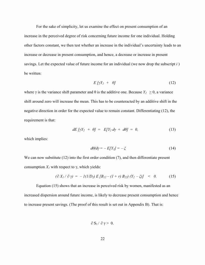
For the sake of simplicity, let us examine the effect on present consumption of an
increase in the perceived degree of risk concerning future income for one individual. Holding
other factors constant, we then test whether an increase in the individual’s uncertainty leads to an
increase or decrease in present consumption, and hence, a decrease or increase in present
savings. Let the expected value of future income for an individual (we now drop the subscript i )
be written:
E [γY2 + θ] (12)
where γ is the variance shift parameter and θ is the additive one. Because Y2 > 0, a variance
shift around zero will increase the mean. This has to be counteracted by an additive shift in the
negative direction in order for the expected value to remain constant. Differentiating (12), the
requirement is that:
dE [γY2 + θ] = E[Y2 dγ + dθ] = 0, (13)
which implies:
dθ/dγ = – E[Y2] = – ξ (14)
We can now substitute (12) into the first order condition (7), and then differentiate present
consumption X1 with respect to γ, which yields:
(∂ X1 / ∂ γ) = – 1(1/D2) E [B12 – (1 + r) B22) (Y2 – ξ)] < 0. (15)
Equation (15) shows that an increase in perceived risk by women, manifested as an
increased dispersion around future income, is likely to decrease present consumption and hence
to increase present savings. (The proof of this result is set out in Appendix B). That is:
∂ S1 / ∂ γ > 0.

23
One implication of the results of this non-pooled household savings model is that
individual saving rates are affected not only by the income level and the interest rate in a given
time period, but also by the person’s perceived interests (Π) and perceived risks (Ξ). Insofar as
women’s perceived interests and risks differ from men’s, they are likely to save at a different rate
than men. This implies that an increase in women’s share of income is likely to affect household
saving rates and, by consequence, aggregate saving rates through the perceived risk effect (
positive) and the perceived interest effect (ambiguous).
Of course, in many cases, household savings are pooled, and the amount of savings out
of income is likely to be determined as a result of a bargaining process between women and men.
The model in the following section takes up this type of household saving pattern.
B. Nash Cooperative Household Bargaining in Pooled Saving Households
We now consider a two-adult household unit which jointly decides how much savings to
set aside. Specifically, saving decisions, as with expenditure allocations, are determined by the
outcome of bargaining between female and male adult members. Saving, therefore, depends not
only on the household’s total income, but also on which member earns it. Each household
member makes choices about time and resource allocation that influence household well-being.
In a given period, each member has the following simplified agency function:
Β i = Β
i( X , S
i, L
i), i = F, M (17)
where again X is a vector of market goods, S is past saving and L is leisure time. Note that this is
a one-period model, with S an argument in the objective function, under the assumption that
well-being today is determined not only by current access to market goods and leisure, but also

24
by how much one is able to put aside as a precautionary measure.
Individual savings are determined by current money income Y, the interest rate r, and a
vector of gender-differentiated variables Ω that reflect the individual’s perceptions of required
future income needs and stability of income sources, such as owned assets, life expectancy,
bequests to children, and family law, and can be written:
S i = S
i (Y
i, r, Ωi
) (18)
Measuring savings proportionate to income, we do not have any evidence a priori to indicate
whether the average female propensity to save (SF
/YF) is significantly different than men’s
(SM
/YM
). The earlier discussion suggests, however, the possibility that propensities differ, even if
income is controlled for, owing to gender differences in the vector of exogenous factors Ω.
If bargaining between women and men breaks down and there is no cooperation, they
face the following time and income constraints in a given time period:
iii TL =Λ+
(19) and
==+Λ YQw iii pX + S
i , (20)
where Λ is paid labor time, T is total waking hours per day (excluding time spent in home
production and personal care), w is the market wage rate, Q is non-wage income from assets,
including past savings, and p is a vector of market good prices.
The decision on whether or not to cooperate depends on the net gain or loss that
cooperation confers to each individual.25
To specify the net gains or loss from cooperation, we
write indirect objective functions for women and men which indicate their "threat points" gained
25
The nature of the net loss (or gains) from cooperation governs the bargaining process and strongly
influences the outcome. It reflects that person’s vulnerability or strength in “bargaining,” as Sen (1990: 135) puts it.

25
independent of cooperation, as:
V i = V
i ( w
i, p
, Q
i, α ). (21)
The V’s in (20) are influenced by the individual's market wage, prices, assets (including past
savings), and a vector of gender environmental parameters (GEPs) α.26
Women and men choose to cooperate if Bi – V
i > 0, that is, if there are gains to
cooperation. In the event of cooperation, the household maximizes a joint welfare function:
N = [B F
– V F]ψ [B
M – V
M]
1-ψ , 0 < ψ < 1 (22)
where the parameter ψ reflects female "voice" or bargaining power, and this acquires the value
of 0 where there is patriarchal dominance and 0.5 when household decision-making is
characterized by equal bargaining power. Households maximize the joint well-being function,
subject to household income and time constraints, derived from combining (19) - (20) or:
p X + S F
+ S M
= wF
ΛF + w
M ΛM
+ QF
+ QM
. (23)
A set of demand functions for the vector of X’s, S’s, and L's can be derived from the
constrained maximization problem as follows:
X* = X (p, w
i, Q
i, r, Ω i
, α , ψ
) (24)
Si*
= Si (p, w
i, Q
i, r, Ω i
, α, ψ) (25)
Li*
= Li (p, w
i, Q
i, r, Ω i
, α ,ψ) (26)
Note that demand functions depend not only on prices and income but also on GEPs and the
26
As noted earlier, GEPs influence the individual’s fallback position, should cooperation fail. These
include employment and other income-earning opportunities, divorce laws, and access to social support systems.
Note that the important distinction between Ω and α is that the former refers to external factors affecting future
social and economic well-being, and the latter refers to those influencing current well-being. This does not preclude
that some elements of vector Ω may be common to α.

26
person’s individual bargaining power.
Using the above frameworks, in this paper we jointly test two propositions. We test
whether women and men have different preferences with regard to saving, as suggested by the
individual savings behavior model. Second, we test, from equation (25), whether a shift in
women’s bargaining power in a pooled-savings household influences the rate of saving out of
household income, and hence aggregate saving. Note that if the first proposition does not hold,
then shifts in female bargaining power that raise ψ will not affect household saving rates.
IV. Empirical Analysis of Aggregate Saving
The theoretical models outlined in equations (1) - (26) provide the framework for an
empirical model of the determinants of household saving rates. The first model indicates why
women’s saving propensities may differ from men’s. It suggests that the effect of women’s share
of income (or total wage bill) on household saving in the case of non-pooled savings households
depends on the relative strength of the positive perceived risk effect and the ambiguous
perceived interest effect. The second model shows how factors that affect women’s relative
bargaining power may influence saving rates in pooled-savings household. In the empirical
analysis that follows, we frame our discussion around these two cases.27
Before proceeding,
however, it is useful to specify the determinants of “voice” or female bargaining power, ψ,
described in the Nash cooperative bargaining model. As noted, determinants of female
27
As will be clear below, there is overlap in the factors that raise women’s bargaining power in pooled
savings households and those that exert a positive effect on women’s relative income in non-pooled savings
households. If, in both cases, overall, women tend to save more than men, then women’s share of the total wage bill
will have a positive effect on the aggregate saving rate. The reverse will hold if, overall, women save less than men
as a percentage of income.

27
bargaining power have generally been related to women’s control over resources, such as assets.
The most commonly used measures are women's share of income and assets at marriage
including women's educational attainment or human capital relative to men's. Proxies for
women’s fallback position in terms of income (call this female relative earnings or FY),
therefore, are required for estimation of empirical models. One possibility is the economy-wide
or aggregate female share of the total wage (FSHW), measured as the ratio of average female
earnings to the sum of average female and male earnings or:28
FSHW = [WF /(WF + WM )]
where WF and WM are average female and male earnings, respectively. An alternative measure
of income earning abilities is women’s share of the wage bill (WSH), measured as the ratio of
average female to male wages multiplied by women’s share of employment or:
WSH = RW * ρ
where RW = WF /WM , and ρ is women’s share of manufacturing jobs. This measure takes into
account not only relative wages but also women’s access to jobs.29
An increase in the size of
each of these variables is expected to produce, on one hand, a positive effect on female
bargaining power in the case of pooled-saving households. On the other hand, it has an
ambiguous effect on the level of present consumption to the extent that women have different
perceived interests than men.
With regard to assets and resources at marriage, a commonly used measure is the gap
28
There are, of course, numerous alternative ways to measure gender wage differences, such as [Ln (WM ) –
Ln (WF])]. Experimentation with other measures provided similar results in the empirical analysis.
29 Because we are using aggregate rather than micro-level data, the two variables that we identify as
exogenous measures of household bargaining power (FSHW and WSH) might also be considered to be GEPs,
leading to some overlap of ψ and α in the empirical analysis.

28
between male and female educational attainment or human capital (DHK) since this reflects
gender differences in access to potential income and a sense of personal efficacy.30
A reduced
form equation for the determinants of female bargaining power can be written as:
(+) (–)
ψ = ψ (FY, DHK) (27)
where DHK is measured as HKM – HKF or the difference between men’s and women’s
educational attainment. Hypothesized signs are noted above the variables.
We now want to test whether increases in women’s share of discretionary income and
bargaining power influence household saving rates. We do this, using aggregate data, and
controlling for other factors that may affect saving propensities. Modifying equation (25) to
represent savings as a share of income, the equation to be estimated is:31
qj = α j + β1j PCY + β2j ADR + β3j FY + β4j DHK + φj σj + εj (28)
qj is saving as a share of income;
PCY is per capita income;
ADR is the age dependency ratio;
FY relative female/male income measure
30
It may be questioned whether in fact education affects women’s bargaining power within the household
in a way not already captured by income. A few studies such as King (1990) explore the relationship between
education and decisionmaking power within the household. King proposes that when the educational gap between
husband and wife is wide, the wife’s role in decisionmaking is limited. An increasing number of studies show that
education can alter women’s self-confidence, self-esteem and notions about their roles in society but the impact of
education is mitigated by a number of social and cultural variables (Archaya and Bennett 1981, Alo and Adjibeng-
Asem 1988 and Floro and Wolf 1990). Nonetheless, the availability of employment is perceived to be a necessary
ingredient that interacts with the skills and attitude changes produced by education , leading to increased
decisionmaking role of women.., Hence, if employment opportunities are greater for more educated workers, again
women’s bargaining power improves as their educational attainment rises.
31
Unfortunately, we lack data on Q (non-wage income) and the full array of GEPs, which may lead to
omitted variable bias. Nor do we have information that would allow us to distinguish between female and male rates
of return on assets (r). Inflation and interest rates in equation (25) do not show up in equation (28) but are added as
control variables to the basic model sequentially, as is shown below. The Ω from equation (25) represents the factors
that may influence women to save at a different rate than men, given different expectations about future income. If
women’s and men’s Ω’s differ, we would expect them to have differing saving propensities as shown in the non-
pooled savings model. We do not, however, have data on Ω.

29
σj is a vector of country dummies;
εj is the error term; and
αj, β1j, β2j, β3j, β4 j, and φj are parameters to be estimated.
In particular, we test here for the determinants of saving as a share of household income,
or qS = S/Y. We focus on the effects of relative female bargaining power which influence saving
rates in pooled-savings households. Income and age dependency ratios are controlled for, under
the assumption that saving rates are influenced in Keynesian fashion by the level of income as
well as by life cycle factors. The remaining variables test for the effect of female relative income
and, by consequence, bargaining power on saving rates. If β3j = β4j = 0, either female and male
propensities to save are identical, and/or households may be unitary decision makers.
Conversely, if β3 ≠ β4 j ≠ 0, then saving propensities differ and changes in female bargaining
power influence household saving rates. Note that we do not have data that allow us to
distinguish between non-pooled savings versus pooled-savings households. We therefore cannot
discern the extent to which whether female relative income and education variables improve
ability to save, or bargaining power within the household.
C. Specification of the Aggregate Saving Model
The empirical model we test uses cross-country time-series data. Absence of reliable
cross-country household-level data on saving, however, requires that we use aggregate data
sources. We therefore use the domestic saving rate, obtained from national income accounts,
which is comprised of household saving, business saving, and government saving as a share of
GDP. In order to test an aggregate saving model, we must control for additional factors
(discussed in Section II and in greater detail in Appendix A) that influence aggregate saving.
The first model (Model I) adopts the absolute income approach and is equivalent to the

30
household model in equation (28):32
DSRit = αo + α1FYit + α2 DHKit + α3 ADRit + α4 PCYit + θit (29)
where DSR is the domestic savings rate as a percent of GDP, FY is a relative income measure to
capture female bargaining power, perceived risks and interests, i is country, t is time, and θ is the
random error. (For a complete listing of all variables and their codes, see Appendix C). We test
three gender versions of this and subsequent models, using the following measures of FY: (1)
female share of the wage (FSHW); (2) a decomposition of the female share of the wage bill, or
the relative female/male wage (RW) and the female share of employment (ρ); and (3) the female
share of the wage bill (WSH).
The second model takes into account life-cycle influences on savings. Here, saving
behavior is assumed to depend positively on the growth rate of GDP, which can be decomposed
into the growth rate of per capita income (PCY1) and the population growth rate (POP1). We test
both versions, or Model IIa and IIb, respectively as follows:
DSRit = βo + β1 FY it + β2 DHKit + β3 ADR it + β4 RGDP1it + β5 PCYit + εit (30a)
DSRit = ζo + ζ1 FY it + ζ2 DHKit + ζ3 ADR it + ζ4 PCY1it + ζ5 POP1it +
ζ6 PCYit + φit (30b)
The third model expands on Models I and II, incorporating factors that influence the
willingness to save. Model IIIa includes a measure of the real interest rate (RIR), which should
induce households to save more if the substitution effect dominates the income effect. Also, the
degree of financial development, measured as money and quasi money as a share GDP (M2) is
32
Some studies include a measure of income squared (PCYSQ) to take account of non-linearities. We do
not find evidence of non-linearities in our sample, and therefore omit PCYSQ. (See the next section on this point).

31
employed. Inflation (INF) which acts as a tax on savings and therefore is expected to have a
negative sign, is included in the model. Tax revenue as a share of GDP is incorporated
(TAXREV) to capture the effect of government saving and taxation on saving. Finally, the
natural logarithm of the terms of trade index (TOT) is included, and is assumed to have a
positive effect on saving. Model IIIa is:
DSRit = δo +δ1 FYit + δ2 DHKit + δ3 ADRit + δ4 PCYit + δ5 RIRit + δ6 M2it + δ7 INFit
+ δ8 TAXREVit + δ9 TOTit + ηit (31a)
Finally, Model IIIb augments the life-cycle model and, in addition, includes the same
willingness-to-save variables used in Model IIIa or:
DSRit = γ0 + γ1 FYit + γ2 DHKit + γ3 ADRit + γ4 PCY1it + γ5 RIRit+ γ6 INFit + γ7 M2it
+ γ8 TAXREVit + γ9 TOTit + γ10 RGDP1it + υit (31b)
V. Econometric Tests and Results
The sample is comprised of a set of semi-industrialized countries for which gender-
disaggregated wage data are available. The sample was selected from middle-income countries
as defined by the World Development Report 1998. Future research might usefully expand this
data set to include industrialized countries. At this juncture, however, our goal was to examine
behavior in countries that were broadly similar in stage of development. The country sample is
provided in Appendix D.
A. The Data
The domestic savings rate, as noted above, is measured as a ratio to GDP. GDP is
measured in 1985 prices and from this, growth rates are calculated for the sample countries. Per

32
capita income data are from the PENN World Tables and are measured in international prices.
The education variables are from Barro and Lee (1996), and DHK is measured as the difference
in average years of secondary education attained by males and females 15 and older.33
The
remaining macro-level variables, described above, are from the World Bank’s World
Development Indicators and the IMF and are measured in a straightforward manner.
Wage and employment data are for the manufacturing sector only and are from the
International Labor Organization (various years). With regard to the wage data, maximum
coverage is from 1975-95, with many countries having shorter coverage. Manufacturing sector
employment data are used rather than economy-wide data since coverage for the latter is not as
broad, and several countries would have dropped out of the sample.
Some cautions about the data should be noted. First, while the broadest period of analysis
is 1975-95, data coverage varies, resulting in variations in sample sizes and thus unbalanced
panels.34
Second, in most cases, the earnings data are corrected for hours worked, but some are
not. Further, these data take into account only women’s and men’s formal employment and wage
earnings in the manufacturing sector, serving only as proxies for economy-wide earnings.35
There are two reasons this may not be cause for significant worry. First, the panel data
estimations capture variation over time, and sectoral gender wage gaps may trend in a similar
fashion. Second, any random measurement error in these variables tends to have a downward
33
Education was alternatively measured as total years of educational attainment by sex. Results, available
upon request, are similar to those obtained using years of secondary education.
34 Hussein and Thirlwall (1999) note, however, that variation in the sample size becomes a useful test of
robustness, depending on whether significance of key variables changes as sample size changes.
35 Consequently, we make the implicit assumption that trends in FY in the manufacturing sector track those
in other sectors of the economy.

33
bias on their coefficients. Therefore any evidence that gender is a significant factor influencing
saving rates may actually be understated.
A third note of caution relates to the aggregate saving data which often have problems of
consistency and reliability. Since gross domestic data is derived from national income accounts,
one may expect measurement errors due to inaccuracies in both investment and balance-of-
payments data, producing a downward bias on coefficients as well. As Fry (1995) notes, the
caveats regarding data inaccuracies need not necessarily lead to misleading econometric results,
provided that the saving data biases are constant over time and the errors are random. In
addition, the use of pooled time-series data, which yields a large number of observations, permits
behavioral relationships to be detected, even though non-trivial random errors in the data may
exist.
Finally, it may be difficult to disentangle the separate effects on saving of the gender
education gap (DHK) and earnings shares (FY) on saving since these variables are likely to be
collinear. Table 1 provides a correlation matrix of the relevant variables. While there is some
evidence of multicollinearity between these variables, education and relative income variables
are not perfect substitutes. This is not surprising since substantial evidence indicates that wage
payments in a number of the countries studied diverge from measured indicators of productivity,
such as education, due to discrimination in labor markets (Behrman and Zhang 1995; Birdsall
and Behrman 1991; Horton 1996; Psacharopoulos and Tzannatos 1992). Further, educational
differences may have implications for men’s and women’s outside options in the marriage
market while wages reflect chances in the labor market. We therefore chose to include both
variables.

34
B. Characteristics of Sample Data
Figures 1 and 2 present time series data of the gender variables used in this analysis for
selected countries. The data exhibit substantial variation both across countries and over time in
women’s share of the wage and the wage bill. Given this, if there are detectable differences in
saving propensities by gender, we would anticipate a significant effect of the gender distribution
of wages (or the wage bill) on aggregate saving. Table 2 gives summary data on the variables
used in the econometric analysis, averaged for the period 1975-95. Figure 3 provides a look at
the relationship between the dependent variable, the domestic savings rate (DSR), and the level
of per capita income against DSR. The data exhibit a positive relationship, but indicate little
evidence of non-linearities.
C. Econometric Results
The regressions are conducted with panel data to capture the effect of changes in
variables within countries over to time to account for time-varying country-specific effects.
Regressions are estimated using a two-way error components model. The basic model can be
summarized as:
Yit = α + Xit β + υ it
where the error term υit has three components:
υit = μi + λt + ε it.
Here μ i captures the country specific-effects while λ t represents time-varying effects. Country
(fixed) effects control for unobserved time-invariant differences that might affect saving.
Several issues need to be considered in estimation: stationarity, heteroskedasticity,
autocorrelation, and endogeneity. In this analysis, many of the variables are expressed as ratios,

35
and are thus stationary in the long run. Two exceptions are TOT and INF which are transformed
into first differences. Heteroskedasticity problems are frequently encountered with cross-
sectional data, and therefore our regressions use GLS, with cross-sectional weights derived from
the residual cross-sectional standard deviations. While this procedure corrects for
heteroskedasticity across countries, a more general form is necessary to allow variances within a
cross section to vary over time. This was done by obtaining standard errors in accordance with
White's variance-covariance matrix in all regressions. We corrected for autocorrelation using an
autoregressive process modeled as an AR(1) with a common country coefficient. In separate
regressions, reported in Appendix E, the lagged dependent variable was included as a regressor.
This reflects that adjustment may take time, and also addresses the autocorrelation problem.
Some right-hand side variables might potentially be endogenous. In particular, the gender
variables may be simultaneously determined by the growth rate of GDP. To check for this,
Hausmann tests were run on Models I-III with the results indicating no evidence of endogeneity
for either gender variable.36
Table 3 summarizes the results obtained from the generalized least squares (GLS)
estimates of Model 1. Equation 1 estimates the basic absolute income model, which is the same
as the household model in equation (28). The coefficient on FSHW is positive and significant,
indicating that a higher relative wage for women raises the aggregate saving rate. As expected
the education gap has a negative sign, indicating that the wider the gap between male and female
secondary educational attainment, the lower the aggregate saving rate. The age dependency ratio
36
This was done by regressing DSR on all independent variables (the “constrained” model). The “suspect”
variable (each of the gender variables) was then regressed on all exogenous variables. The resulting fitted values
were then added to the constrained model. T-tests of the significance of that variable did not support the hypothesis
of endogeneity of gender variables.

36
coefficient is negative as would be expected, but is insignificant. Finally, the level of per capita
income is positive and significant. In equation 2, we decompose the female share of the wage bill
into two parts, RW, the relative female/male wage, and ρ, the female share of employment. Each
of these variables is positive and significant. In this case, DHK becomes insignificant, but
coefficients on the remaining variables are stable. Finally, equation 3 uses the female share of
the wage bill, and this is also positive and significant.
The results of estimating the Life Cycle Model (Model II) are shown in Table 4. For
Model IIa, which includes the growth rate of GDP as an explanatory variable, in equations 1 and
2, the gender income variables are positive and significant, while in equation 3, the female share
of the wage bill is positive but insignificant. PCY is robust to this alternative specification, while
again, DHK is only significant and negative in equation 1. RGDP1 is positive and significant in
equation 1, but changes sign in equation 2, and is insignificant in equation 3. Model IIb replaces
RGDP1 with POP1 and PCY1, and gives results shown in equations 4-6. The gender income
variables and PCY are robust to this alternative specification, while POP1 is negative as would
be expected and PCY1 performs perversely or is insignificant.
Table 5 provides the results of testing modified versions of Models I and II. In Model
IIIa, we add financial and macroeconomic variables. In equation 1, the coefficient on FSHW is
positive and significant but is reduced in size by about one half from Models I and II. PCY
continues to perform robustly. All of the financial and macroeconomic variables with the
exception of the terms of trade variable are significant. Interestingly, the sign on the real interest
rate variable is negative, a finding that is consistent with Keynesian and structuralist
perspectives. The robustness of the FSHW variable as the sample size changes is notable. DHK,

37
however, changes sign and continues to be insignificant in all versions of Model III. The female
share of the wage bill (WSH) does not, however, perform so robustly, nor do its decomposed
components (equations 2 and 3). Model IIIb adds RGDP1 as a life cycle variable. The FSHW
variable as well as the financial and macroeconomic variables are again robust, but RGDP1 is
insignificant. Finally, in equations 5 and 6, again the decomposed FSHW and the WSH are
insignificant, and in one case, change signs. Also, the low Durbin-Watson statistic makes the
estimates in this equation unreliable.37
In sum, two variables perform robustly in all three models in this analysis, PCY and
FSHW. In Models I and II, WSH as well as its decomposed parts also performed as predicted by
the household bargaining model. The insight offered by the results obtained from decomposing
the wage share is that even if relative wages remain constant, women’s greater access to
employment improves their outside options sufficiently to raise bargaining power and influence
saving rates.
The education variable performed less robustly than the income variables, although this
may be in part explained by multicollinearity among these variables. (Running regressions with
the education variable as the only bargaining power variable yielded slightly more consistently
significant negative coefficients). Table 6 summarizes the econometric results obtained of the
gender bargaining power variables.
The preliminary evidence on the role of gender in determining aggregate saving suggests
measures of women’s access to outside income raises the aggregate saving rate. The size of the
effect is not insignificant. Though it varies in our estimates, consider, for example, the results
37
Similar results were obtained using PCY1 and POP1 in place of RGDP1.

38
given in Table 4. There we see that a one percentage point increase in women’s share of the
wage raises aggregate saving by roughly a quarter percentage point. Similarly, a percentage
point increase in women’s share of income raises aggregate saving by about one sixth of a
percentage point.
These results are suggestive of differential savings behavior at the household level, with
women’s propensity to save higher than that of males at least for this set of countries. These
results are also consistent with a growing body of research that suggests that gender is an
important macroeconomic variable, and links this to micro-level, household behavior.
VI. Conclusion
This paper explores the role that gender plays in influencing aggregate saving rates for a
set of semi-industrialized countries. These countries have increasingly relied on female labor in
their export manufacturing sectors. A question of interest is whether increases in women’s wages
relative to men’s as well as increases in their share of income have affected aggregate saving
rates. Presupposed in this question is that women and men have differing propensities to save
due to variations in perceived risks and interests and in gender-related external factors that affect
savings behavior.
This paper is exploratory in the sense that little prior evidence existed to indicate whether
higher relative wages and income for women will raise or lower saving rates—whether the effect
will be so negligible as to be undetectable. Preliminary evidence provided here using a panel
data set is consistent with the hypothesis that an increase in women’s discretionary income and
bargaining power raises household saving and therefore aggregate saving rates. These results are

39
of interest in that they imply an aggregate role for micro-level gender relations at the household
level. A deeper understanding of the determinants of saving rates at the household level is
especially useful in planning for savings mobilization and in the formulation of financial and
investment policies.

40
REFERENCES
Acharya, Meena and Lyn Bennett (1981). "Women and the Subsistence Sector: Economic
Participation and Household Decision-making in Nepal," World Bank Staff Working
Paper No. 526, World Bank, Washington, D.C.
Adams, Dale and Delbert Fitchett, eds. (1992). Informal Finance in Low-Income Countries,
Westview Press, Boulder.
Agarwal, Bina (1995). A Field of One’s Own: Gender and Land Rights in South Asia,
Cambridge University Press, Cambridge.
Aghevli, Bijan, James Broughton, Peter Montiel, Delano Villanueva, and Geoffrey Woglom
(1990). “The Role of National Saving in the World Economy: Recent Trends and
Prospects,” IMF Occasional Paper No. 67, International Monetary Fund, Washington
DC.
Akyűz, Yilmaz (1991). “Financial Policies for Industrialization and Development: Reflections
on Financial Deepening and Efficiency,” in Machiko Nissanke and Adrian Hewitt (eds.),
Economic Crisis in Developing Countries: New Perspectives on Commodities, Trade and
Finance, Pinter, London.
Alo, O. and S. Adjebeng-Asem (1988). "Women and National Development: A Socio-Cultural
Analysis of the Nigerian Experience." In M. F. Abraham and P. S. Abraham (eds.),
Women, Development and Change: The Third World Experience, Wyndham Hall Press,
Brystol, Indiana.
Bajtelsmit, Vickie and Alexandra Bernasek (1996). “Why Do Women Invest Differently Than
Men?” Financial Counseling and Planning 7.
Bajtelsmit, Vickie and J. Van Derhei (1997). “Risk Aversion and Pension Investment Choices,”
in Michael S. Gordon, et. al. (eds.), Positioning Pensions for the Twenty-First Century,
University of Pennsylvania Press, Philadelphia, pp. 45-66.
Barke, R, H. Jenkins-Smith and P. Slovic (1997). “Risk Perceptions of Men and Women
Scientists,” Social Science Quarterly 78 (1): 167-176.
Barro, Robert and Jong-Wha Lee (1996). “International Measures of Schooling Years and
Schooling Quality,” American Economic Review 86 (2): 218-223.
Behrman, Jere and Zhang, Z (1995). “Gender Issues and Employment in Asia,” Asian
Development Review 13 (2): 1-49.
Benería, Lourdes and Martha Roldan (1987). The Crossroads of Class and Gender: Industrial
41
Homework, Subcontracting and Household Dynamics in Mexico City, University of
Chicago Press, Chicago.
Bernasek, Alexandra (2000). “Gender, Risk and Investment: A Feminist Perspective,” paper
presented at the Annual IAFFE Conference, Istanbul, Turkey, August 15-17, 2000.
Birdsall, Nancy and Jere Behrman (1991). “Why Do Males Earn More Than Females in Urban
Brazil: Earnings Discrimination or Job Discrimination,” in Nancy Birdsall and Richard
Sabot (eds.), Unfair Advantage: Labor Markets Discrimination in Developing Countries,
World Bank, Washington, D.C., pp. 147-69.
Blumberg, Rae Lesser (1988). “Income Under Female Versus Male Control: Hypotheses From a
Theory of Gender Stratification and Data From the Third World,” Journal of Family
Issues 9 (1): 51-84.
Boskin, Michael (1978). “Taxation, Saving, and the Rate of Interest,” Journal of Political
Economy 86 (2): S10-S27.
Brenner, R., Marcel Dagenais, and C. Montmarquette (1994). “An Overlooked Explanation of
the Declining Saving Rate,” Empirical Economics 19 (4): 629-37.
Callen, Tim and Christian Thimann (1997). “Empirical Determinants of Household Saving:
Evidence from OECD Countries,” IMF Working Paper 97/181, International Monetary
Fund, Washington, D.C.
Caroll, Christopher and D. Well (1993). “Saving and Growth: A Reinterpretation,” NBER
Working Paper No. 4470, National Bureau for Economic Research, Cambridge, MA.
Dayal-Gulati, Anuradha and Christian Thimann (1997). “Saving in Southeast Asia and Latin
America Compared: Searching for Policy Lessons,” IMF Working Paper 97/110,
International Monetary Fund, Washington, D.C.
Deaton, Angus (1990). “Savings in Developing Countries: Theory and Review,” in Stanley
Fischer and Dennis de Tray (eds.), Proceedings of the World Bank Annual Conference on
Development Economics 1989, World Bank, Washington D.C.
Deaton, Angus and Christina Paxson (1997). “Growth, Demographic Structure and National
Saving in Taiwan,” Working Paper for Princeton University, Research Program in
Development Studies.
(1998). “Saving and Growth: Another Look at the Cohort Evidence,” Working Paper for
Princeton University, Research Program in Development Studies.
de Melo James and James Tybout (1986). “The Effects of Financial Liberalization on Saving and
42
Investment in Uruguay,” Economic Development and Cultural Change 34 (3): 561-587.
Deolalikar, Anil and Vijayendra Rao (1998). “The Demand for Dowries and Bride
Characteristics in Marriage: Empirical Estimates of Rural South-Central India,” in R.
Sudharshan (ed.), Gender, Population and Development, Oxford University Press, New
Delhi.
Dornbusch, Rudiger and Alejandro Reynoso (1989). “Financial Factors in Economic
Development,” American Economic Review 79 (2): 389-444.
Doss, Cheryl. (1996). “Women’s Bargaining Power in Household Economic Decisions:
Evidence from Ghana,” Department of Applied Economics Staff Paper P96-11,
University of Minnesota, July.
Edwards, Sebastian (1995). “Why Are Savings Rates So Different Across Countries? An
International Comparative Analysis,” NBER Working Paper No. 5097, National Bureau
of Economic Research, Cambridge, Massachusetts.
Feldstein, Martin and Philippe Bacchetta (1991). “National Saving and International
Investment,” in B. Douglas Bernheim and John B. Shoven (eds.), National Saving and
Economic Performance, Chicago University Press for NBER, pp. 201-226.
Fleck, Susan (1998). “Choice or Bargain? Married Women’s Labor Force Participation in
Honduras,” Ph.D. dissertation, American University, Washington D.C.
Floro, Maria and Joyce Wolf (1990). The Economic and Social Impacts of Girls' Primary
Education in Developing Countries, Advancing Basic Education and Literacy (ABEL)
Project, U.S. Agency for International Development, Washington, DC.
Floro, Maria Sagrario (1995). “Women’s Well-Being, Poverty, and Work Intensity,” Feminist
Economics 1 (3): 1-39.
Folbre, Nancy (1997). “Gender Coalitions: Extrafamily Influences on Intrafamily Inequality,” in
Lawrence Haddad, John Hoddinott, and Harold Alderman (eds.), Intrahousehold
Resource Allocation in Developing Countries: Models, Methods, and Policy, Baltimore
and London, Johns Hopkins University Press for the International Food Policy Research
Institute, pp. 263-74.
Flynn, J., P. Slovic, and C. K. Merck (1994). “Gender, Race and Perception of Environmental
Health Risks,” Risk Analysis 16 (6): 1101-1108.
Fry, Maxwell J (1978). “Money and Capital or Financial Deepening in Economic
Development?,” Journal of Money Credit and Banking 10 (4): 464-475.

43
(1984). “Saving, Financial Intermediation and Economic Growth in Asia,” Asian
Development Review 2 (1):. 82-91.
_____ (1995). Money, interest, and banking in economic development, Johns Hopkins
University Press, Baltimore and London.
(1996). “Finance and Growth in Pacific Basin Developing Countries,” in Niels Hermes
and Robert Lesnick (eds.), Finance Development and Economic Growth, Routledge,
London, pp. 138-160.
Fry, Maxwell and Andrew Mason (1982). “The Variable Rate of Growth Effect in the Life Cycle
Saving Model: Children, Capital Inflows, Interest and Growth in a New Specification of
the Life Cycle Model Applied to Seven Asian Countries,” Economic Inquiry 20 (3): 426-
42.
Ghate, Prabhu (1992). Informal Finance: Some Findings from Asia, Oxford University Press and
Asian Development Bank, Manila.
Giovannini, Alberto (1983). “The Interest Elasticity of Savings in Developing Countries: The
Existing Evidence,” World Development 11 (7): 601-607.
____ (1985). “Saving and the Real Interest Rate in LDCs,” Journal of Development Economics
18 (2 and 3): 197-217.
Goetz, Anne Marie and Rina Sen Gupta (1996). “Who Takes the Credit? Gender, Power, and
Control Over Loan Use in Rural Credit Programs in Bangladesh,” World Development 24
(1): 45-63.
Greenhalgh, Susan (1985). “Sexual Stratification: The Other Side of Growth with ‘Equity’ in
East Asia,” Population and Development Review 1 (2): 265-314.
Gugerty, May Kay (1999). “Preliminary Evidence on Rotating Savings and Credit Associations
(ROSCAs) in Kenya: You Can’t Save Alone,” Mimeo, Harvard University.
Gupta, Kanhaya L. (1987). “Aggregate Savings, Financial Intermediation, and Interest Rate,”
Review of Economics and Statistics 69 (2): 303-17.
Guyer, Jane (1988). “Dynamic Approaches to Domestic Budgeting: Cases and Methods from
Africa,” in Daisy Dwyer and Judith Bruce (eds.), A Home Divided: Women and Income
in the Third World, Stanford University Press, Palo Alto, pp. 155-172.
Haddad, Lawrence and John Hoddinott (1991). “Gender Aspects of Household Expenditures
and Resource Allocation in the Côte d’Ivoire,” Oxford Applied Economics Discussion
Paper 112.

44
Handa, Sudhanshu (1994). “Gender, Headship and Intra Household Resource Allocation,” World
Development 22 (10): 1535-1547.
Higgins, Matthew and Jeffrey Williamson (1997). “Age Structure Dynamics in Asia and
Dependence on Foreign Capital,” Population and Development Review 23: 261-93.
Hinz, Richard, David McCarthy, and John Turner (1996). “Are Women Conservative Investors?:
Gender Differences in Participant-Directed Pension Investments,” in Michael Gordon,
Olivia Mitchell, and Marc Twinney (eds.), Positioning Pensions for the Twenty-First
Century, University of Pennsylvania Press, Philadelphia, PA, pp. 145-156.
Horton, Susan (1996). Women and Industrialization in Asia, Routledge, London and New York.
Hulme, David and Paul Mosley (1996). Finance Against Poverty, Routledge, London.
Hungerford, Thomas (1999). “Saving For a Rainy Day: Does Pre-Retirement Access to
Retirement Savings Increase Retirement Saving?,” Mimeo, Social Security
Administration.
Hussein, Khaled and A. P.Thirwall (1999). “Explaining Differences in the Domestic Savings
Ratio Across Countries: A Panel Data Study,” Working Paper, University of Kent at
Canterbury.
International Labour Organization. Yearbook of Labour Statistics (various years), Geneva.
Jianakoplos, Nancy and Alexandra Bernasek (1998). “Are Women More Risk Averse?,”
Economic Inquiry 36: 620-630.
Kabeer, Naila (2000). The Power to Choose: Bangladeshi Women and Labour Market Decisions
in London and Dhaka, Verso, London.
Katz, Elizabeth (1991a). “Breaking the Myth of Harmony: Theoretical and Methodological
Guidelines to the Study of Rural Third World Households,” Review of Radical Political
Economics 23 (3 and 4): 37-56.
____ (1991b). “Intrahousehold Resource Allocation in the Guatemalan Central Highlands: The
Impact of Non-Traditional Agricultural Exports,” paper presented at the Latin American
Studies Association, Washington DC.
Kim, Seung-Kyung (1997). Class Struggle or Family Struggle?: The Lives of Women Factory
Workers in South Korea, Cambridge University Press, Cambridge, UK.

45
King, Elizabeth (1990). Educating Girls and Women: Investing in Development, World Bank,
Washington, DC.
Kumar, Shubh (1978). “Role of the Household Economy in Child Nutrition at Low Incomes: A
Case Study in Kerala,” Occasional Paper No. 95, Department of Agricultural Economics,
Cornell University, Ithaca, NY.
Leff, Nathaniel (1969). “Dependency Rates and Saving Rates,” American Economic Review 59:
886-96.
Leland, Hayne (1968). “Saving and Uncertainty: The Precautionary Demand for Saving,”
Quarterly Journal of Economics 82: 465-473.
Lundberg, Shelly, Robert Pollak, and Terence Wales (1995). “Do Husbands and Wives Pool
their Resources? Evidence from the U.K. Child Benefit,” Working Paper, University of
Washington, April.
Masson, Paul, Tamim Bayoumi, and Hossein Samiei (1995). “Saving Behavior in Industrial and
Developing Countries,” Staff Studies for the World Economic Outlook, International
Monetary Fund, pp. 1-27.
Modigliani, Franco (1966). “The Life Cycle Hypothesis of Saving, the Demand for Wealth and
the Supply of Capital,” Social Research 33: 160-217.
(1970). “The Life Cycle Hypothesis of Saving and Inter-country Differences in the Saving
Ratio” in Walter Eltis, et. al. (eds.), Induction, Trade and Growth: Essays in Honor of Sir
Roy Harrod, Oxford, pp. 197-225.
(1986). “Life Cycle, Individual Thrift, and the Wealth of Nations,” American Economic
Review 76 (3): 297-313.
Modigliani, Franco and Albert Ando (1957). “Tests of the Life Cycle Hypothesis of Savings:
Comments and Suggestions,” Bulletin of the Oxford Institute of Statistics, pp. 99-124.
Neuhouser, Kevin (1989). “Sources of Women’s Power and Status Among the Urban Poor in
Contemporary Brazil,” Signs 14 (3): 684-702.
Ogaki, Masao, Jonathan Ostry, and Carmen Reinhart (1994). “Saving Behavior in Low- and
Middle-Income Developing Countries: A Comparison,” Working Paper 95/3,
International Monetary Fund, Washington, D.C.
Ostry, Jonathan and Carmen Reinhart (1992). “Private Saving and Terms-of-Trade Shocks:
Evidence from Developing Countries,” IMF Staff Papers, 39: 495-517.

46
Palsson, Anne-Marie (1996). “Does the Degree of Relative Risk Aversion Vary with Household
Characteristics?,” Journal of Economic Psychology 17 (6): 771-87.
Papanek, Hanna and Laurel Schwede (1988). “Women are Good with Money: earning and
Managing in an Indonesian City” in Daisy Dwyer and Judith Bruce (eds.), A Home
Divided: Women and Income in the Third World, Stanford University Press, Palo Alto,
pp. 71-98.
Paxson, Christina (1995). “Saving and Growth: Evidence From Micro Data,” NBER Working
Paper No. 5301, National Bureau of Economic Research, Cambridge, Massachusetts.
Phipps, Shelley and Peter Burton (1998). “What’s Mine is Yours? The Influence of Male and
Female Incomes on Patterns of Household Expenditure,” Economica 65: 599-613.
Psacharopoulos, George and Zafiris Tzannatos (1992). Case Studies on Women’s Employment
and Pay in Latin America, World Bank, Washington, D.C.
Quisumbing, Agnes and John Maluccio (1999). “Intrahousehold Allocation and Gender
Relations: New Empirical Evidence,” Gender and Development Working Paper Series,
No. 2, World Bank, Washington, D.C.
Roldan, Martha (1988). “Renegotiating the Marital Contract: Intrahousehold Patterns of Money
Allocation and Women’s Subordination Among Domestic Outworkers in Mexico City”
in Daisy Dwyer and Judith Bruce (eds.), A Home Divided: Women and Income in the
Third World, Stanford University Press, Palo Alto, pp. 229-247.
Safilios-Rothschild, Constantina (1988). “The Impact of Agrarian Reform on Men’s and
Women’s Incomes in Rural Honduras,” in Daisy Dwyer and Judith Bruce (eds.), A Home
Divided: Women and Income in the Third World, Stanford University Press, Palo Alto,
pp. 216-228.
Sandmo, Agnar (1970). “The Effect of Uncertainty on Saving Decisions,” Review of Economics
and Statistics 37: 353-60.
Schmidt-Hebbel, Klaus, Steven Webb, and Giancarlo Corsetti (1992). “Household Saving in
Developing Countries: First Cross-Country Evidence,” World Bank Economic Review 6
(3): 529-547.
Sen, Amartya (1990). “Gender and Cooperative Conflicts” in Irene Tinker (ed.), Persistent
Inequalities: Women and World Development, Oxford University Press, New York, pp.
123-149.
Smith, Roger (1990). “Factors Affecting Saving, Policy Tools, and Tax Reform: A Review,”
IMF Staff Papers 37 (1): 1-70.

47
Sunden, Annika E. and Brian J. Surette (1998). “Gender Differences in the Allocation of Assets
in Retirement Savings Plans,” American Economic Review 88 (2): 207-211.
Taylor, Lance (1983). Structuralist Macroeconomics: Applicable Models for the Third World,
Basic Books, New York.
Thomas, Duncan (1992). “The Distribution of Income and Expenditure Within the Household,”
IFPRI World Bank Conference on Intrahousehold Resource Allocation: Policy Issues and
Research Methods, Washington D.C.
Thomas, Duncan and Chien-Liang Chen (1993). “Income Shares and Shares of Income:
Empirical tests of Models of Household Resource Allocations,” Working Paper, RAND
Corporation.
Van Wijnbergen, Sweder (1983). “Credit Policy, Inflation, and Growth in a Financially
Repressed Economy,” Journal of Development Economics 13 (1 and 2): 45-65.
Wolf, Diane (1988). “Female Autonomy, the Family, and Industrialization in Java,” Journal of
Family Issues 9 (1): 85-107.
World Bank (1998). World Development Indicators.