The Effects of Short Sale Constraints onDerivative Prices

Roland Nilsson∗

Stockholm School of Economics

June 24, 2003JEL Classification: G12

Abstract

This paper tests the effects of short sale constraints on derivative pricesby considering deviations from put-call parity (PCP). To measure theimpact of short sale constraints I focus on Sweden and a particular periodduring which shorting stocks was almost impossible while at the sametime stock options were traded. I found that the deviations from PCPcorresponding to a short position in the stock were larger in absolutemagnitude during the period when shorting was restricted compared withthe period after. Furthermore, the introduction of futures on individualstocks were also considered. However, futures seem not to significantlyaffect the degree of short constraints in the market. Finally, only for stockoptions that had an underlying share that couldn’t be shorted abroadcould a pattern consistent with a short sale constraint be observed.

1 IntroductionThe base case scenario in most models within financial economics is a world freeof frictions, in particular, a world free of any constraints to the ability of goingshort. Even though constraints on shorting has been considered before, it isonly during the last few years that one seriously started to investigate whetherthis is an innocuous assumption or not. One of the earlier papers on the subjectwas written by Miller (1977), in which he proposes an intuition rather than aformal model of why constraints on shorting could matter. According to Miller isshorting a way for investors that do not own the stock to get their low valuationsof the asset incorporated into the equilibrium price. If shorting is restrictedthose beliefs will not be incorporated and thus leaving the price of the assetelevated above the equilibrium price. Part of this argument has subsequently

∗Roland Nilsson (email: roland.nilsson@hhs.se, phone: +46-8-736 9391, fax: +46-8-312327), PhD student at Department of Finance, Stockholm School of Economics, Box 6501,SE-113 83 Stockholm, Sweden.

1

been formalised in for instance Chen, Hong and Stein (2002). However, in orderfor the argument to go through one has to assume either that there is some limitsto investor’s rationality or some form of limits to information (i.e. investors arenot aware of the fact that certain agents are short sale constrained). If one doesnot impose one of these restrictions the price, given the appropriate informationset, will be unbiased (Diamond and Verrecchia, 1987). The implications of shortconstraints on equities are therefore not completely clear.

For derivatives, on the other hand, since their values are determined byrelying on a replicating portfolio argument where one goes long a portfolio andshort an other, an absolute short constraint on the stock, in case of a stockoption, would imply that the replication argument breaks down. In other words,as opposed to equity there is a very clear cut reasoning behind the effects ofshort sale constraints on stock option prices, which is why this will be the topicof the following paper.

The paper will furthermore focus on the case of Sweden because of the veryspecial institutional setting which prevailed there for a number of years. To bemore specific, between 1980 until the end of 1991 banks and brokerages houseswere forbidden by law to participate in a stock lending/borrowing transaction.They could not be a party in the transaction or bring the two parties, the lenderand the borrower, together. In effect there didn’t exist a market place for lend-ing and borrowing stocks in Sweden during this period. Furthermore, in 1985the derivatives exchange, OM, opened and started to trade stock options. Be-tween 1985 to 1991 the rather unusual situation prevailed in Sweden where stockoptions were traded but the underlying stock was virtually impossible to short.At the end of 1991 the law forbidding banks and brokerages houses to involvethemselves in stock lending and borrowing was abolished and several marketplaces were established. The main purpose of this paper is therefore to investi-gate the effect of short sale constraints on stock option prices by comparing theperiod 1985 to 1991 in Sweden with the period after.

Furthermore, another rather unusual feature to the Swedish derivatives mar-ket is the existence of futures on individual stocks. Whereas most countries havefutures on indices few countries have it on stocks. Since the US Congress only afew years ago passed a law allowing the trade of single-stock futures the effectsof the introduction of such instruments should also be of interest to the USmarket. The reason why any effects at all could be expected from stock-futuresintroduction is the fact that they allow investors to take a short position in thestock. If the cost of this transaction is smaller than the cost of going short, usingthe lending and borrowing market for stocks, then the constraints of shortingwill be reduced. The cost of the transaction should in this context not onlyinclude the direct transaction costs but also legislational aspects as well as liq-uidity etc. The second purpose of this paper will therefore be to investigate theeffect of the introduction of futures on individual stocks.

2

To give a short preview of the results I do find that the shorting constraintincreased the deviations from PCP in the direction corresponding to a shortposition in the stock, while no such increase could be detected for deviationsfrom PCP where a long position in the underlying is required. The introductionof futures however did not seem to have any effect.

Finally, the paper considers stocks which where shortable abroad and thosethat were not shortable abroad separately. The pattern mentioned above wasonly found for the stocks that were not shortable abroad while this was not thecase for the other stocks.1

2 Methodology

2.1 Measuring the Effects of Short Sale Constraints

The effects of short sale constraints could be captured in many ways. Onealternative would be to consider implied volatilities. In the spirit of Black &Scholes (1973) express the value of an European call on a non-dividend payingstock with strike price X as a fraction αt(σ, ·) in the stock, St, and a fractionβt(σ, ·) in a bond. Both fractions depend on the volatility of the derivative anda number of other omitted variables,

ct = αt(σ, ·)St − βt(σ, ·)X

If shorting the stock was impossible then obviously a situation where c <c∗ could prevail, where c∗ is the "true" value of the call. Since ∂ct

∂σ > 0 anundervalued call would imply that the implied volatility also would be too low.This would be what one should be looking for in the data. However, one hasto make a stand on how to define a too low implied volatility and in the endthe method chosen could always, justifiably, be criticized on different grounds.Secondly, the method is model dependent. For these reasons will I insteadchoose an other method by considering deviations from an arbitrage relation

1Only after this project was started did I learn about a paper still in progress by Ofek,Richardson and Whitelaw (2002) which more or less considers the same situation as I do,namely the effect of short sale constraint on option prices by considering deviations from put-call parity. There is one major difference between our studies, however. Ofek, Richardsonand Whitelaw (2002) have to rely on some measure that captures the degree of short saleconstraint in the market. In their paper the measure used is the direct cost of going shortwhich they claim also should be a proxy for how difficulty it is to go short. Since a shortsale constraint is a multidimensional constraint that depends on a number of variables, thedirect cost only being one of them, one can always question whether all important aspectshave been incorporated into the measure. This critique clearly does not apply to this studysince I consider two different regimes that vastly differs in the ease by which one can go short.During one period it is almost impossible, during the second period it is easier to go shortthan it is currently in the US. Furthermore, I do consider the effect of introducing futures aswell as how trade at different exchanges affects the short sale constraint, something they donot.

3

that also involves going short the stock. The relationship chosen will be theput-call-parity, henceforth PCP, which dictates that:

pt − ct + St −Xe−r(T−t) = 0

The effects of an absolute short sale constraint on the stock on the PCPwould be that the following relation could prevail:

pt − ct + St −Xe−r(T−t) > 0 (1a)

where pt is the value of an European put on a non-dividend paying stock, ris the continuously compounded interest rate, T − t is the time to maturity ofboth derivatives and X the strike of both derivatives. Since PCP never will holdexactly because of transaction costs, I will control for most of those to avoid theintroduction of additional noise in my estimations. Consider first a situationwhere pt − ct < Xe−r(T−t) − St in which case one would like to go long theleft hand side and short the right hand side. If after controlling for bid and askprices as well as other transaction costs, OT , the following holds:

Xe−r(T−t) − Saskt − paskt + cbidt −OT < 0 (2)

then there is no room for a profitable transaction. Note that expression (2)involves going long the stock. In the reverse scenario when pt−ct > Xe−r(T−t)−St the following expression dictates the no arbitrage condition:

pbidt − caskt −Xe−r(T−t) + Sbidt −OT < 0 (3)

in which case one is forced to go short the stock. If derivative prices hasto adjust to any change in the price of the underlying and not the other wayaround, any deviation from PCP will imply that the derivatives are mispricedand not the stock. However, it will not be possible to say which one if thederivatives or whether both are mispriced.

Until the end of 1991, a period exactly corresponding to the short sale con-strained period considered in this study, investors were also obliged to pay aturn over tax on stocks and derivatives. This will also be controlled for, seeappendix A for some further details on the adjustment procedure. Finally, com-mission will not be controlled for since the data is unavailable. If, on average,there are differences between the periods this could affect the results.

2.2 Normalisation

To be able to aggregate across companies some form of normalisation procedurehas to be applied. The first method used will be to divide the deviations from (3)and (2) by the strike price. A second version will also be used which follows themethod proposed by Kamara and Miller Jr. (1995), see appendix B for furtherdetails. However, the results from the two different normalisation proceduresare more or less identical and I will therefore continue to normalise by the strikeprice.

4

2.3 American Options

All the stock options traded at OM are of the American type. When the under-lying stock doesn’t pay any dividend the value of an American call is equal tothat of an European call. For the American put however, it could be optimalto exercise the option prematurely, so:

P = p+ EEP

where P is the value of the American put and EEP is the early exercise pre-mium. Equations (2) and (3) has to be adjusted by exchanging p for P −EEP .The early exercise premium is calculated by using a programme by CameronRookley who uses a method proposed by Barone-Adesi and Whaley (1987)2. Itshould be pointed out that this method is model dependent. However, in theend the EEP is very small so even if it were grossly miscalculated this wouldnot change the results.

Deviations from PCP has also been used to approximate the value of EEP ,see Zivney (1991). Also two studies conducted on Swedish data by Engström,Nordén and Strömberg (2000) and Engström and Nordén (2000) has used thesame approach. Obviously by attributing any deviation from PCP to the EEPone assumes that the markets are frictionless. In particular do not short saleconstraints nor poor liquidity play any role for these deviations. This papershows that short sale constraints do matter and that such an assumption there-fore is inappropriate.

2.4 Matching Procedure

PCP involves taking a position in a call and a put with the same strike priceand with the same time to maturity. To match puts and calls the followingmatching procedure was used:

• Among all calls for a given company a given day, take the one with theshortest time to maturity (TTM), as long as the TTM is longer than14 calendar days. The last 14 days have been excluded since strangeprice movements have been documented just prior to the expiration ofthe options (see Day and Lewis, 1988). By focusing on derivatives with ashort TTM I will limit myself to liquid data, the importance of which willbe discussed further on.

• From those calls with the shortest TTM choose the one which has a strikeclosest to the price of the underlying.

• Require further that the strike be in the following range:

−0.1 < ln(X/St) < 0.1 (4)

2See www.cameronrookley.com/options/options.html

5

By imposing this restriction only options that are quite at the money arechosen. Again, this is done in order to restrict the data to the subset which ishighly liquid.

• Given the picked call try to find a put with matching strike and maturity.• Discard any matches where either derivative have zero volume or no quotedclosing price. Also, if there is no price in the underlying asset or the impliedvolatility of the American put could not be found (the programme didn’tconverge to a solution) that matched pair would not be included.

• If during the life time of the derivatives the underlying pays out a dividendthe observation is discarded. The main reason is that the method proposedin Barone-Adesi and Whaley (1987) can handle a continuous dividendpayment but is much less applicable to discrete ones.

To increase the number of matched observations an adjusted matching pro-cedure was also tried. The adjusted procedure works exactly as the above onewith the only exception that instead of just taking the call which is most at themoney and try to find a matching put, the next closest at the money call is alsoconsidered, and then the third next closest at the money call and so on as longas bound (4) is not violated.

3 Institutional SettingIn 1980 a law prohibiting banks and brokerage houses to participate in a shortselling transaction was introduced. The ban was lifted 1991-09-01 and the firstmarket for lending and borrowing was introduced in 1991-11-21. This datewill mark the end of the period during which shorting was severely restricted,denoted as period A. During the period 1991-11-22 to 1992-02-05 due to the factthat the lending of a stock was considered to be a realisation from a taxationalpoint of view, virtually no lending took place. In 1992-02-06 this was changedand lending was no longer considered a realisation. This date will mark thebeginning of the period during which shorting was no longer restricted, denotedas period C.The first future on an individual stock was introduced in 1992-07-01 and

the last one, for the firms included in this study, was 1993-11-10. The period inbetween the introduction of futures and the abolishment of the short constraintswill be denoted period B, while the period after is called D, see picture 1 for atime line.

During this period not only the restriction to short was lifted but also severalother restrictions imposed on the financial markets. Until the end of 1992 mostshares had a restricted share which was not tradable by foreigners and a unre-stricted version that for most big companies were traded abroad. For the stockoptions considered in this study some had an underlying which was restricted

6

and some had one which was unrestricted. Since the short sale constraint wasa national matter, the unrestricted shares traded abroad was not subject toany constraint on the foreign exchange, something which will turn out to beimportant for this study.

4 Hypothesis and Confounding FactorsIn this study three hypothesis will be tested for:

Conjecture 1: The magnitude of the deviations from relation (3) are largerduring the period 1985 to 1991 compared to the subsequent period while devi-ations from (2) are the same across periods.

Conjecture 2: The introduction of futures on individual stocks implies areduction of the short constraint in the market and thus smaller deviations fromrelation (3). Again no effect on (2) should be seen.

Conjecture 3: For the unrestricted shares with a significant volume tradedabroad conjecture 1 should not hold.

Although short sale constraints ought to be a major reason to why we ob-serve deviations from PCP, there are several other sources for deviations as well.Suppose that new information first is incorporated into stock prices and onlysubsequently into derivative prices, i.e. stock prices "lead" derivative prices.Since derivative prices will adjust with a time lag, the arrival of new informa-tion to the market will cause deviations from PCP. Short sale constraints should,as in Diamond and Verrecchia (1987), make this adjustment process slower whenshorting the stock is required. If the difference in adjustment speed when short-ing is allowed and when it isn’t is not too great, the arrival of new informationwill in general lead to deviations from PCP in both periods. Therefore the fre-quency of deviations between the periods will most likely not differ. However,this will not be the case for the magnitude. For this reason I will focus on themagnitude of the deviations from PCP rather than the frequency.

Another relevant and very much related topic is liquidity. To take advantageof deviations from PCP it is crucial that all transactions are made simultane-ously since any delay in any of the transactions could imply an unfavourableprice change, precluding an arbitrage transaction. Firstly, variables that havebeen used as proxies for liquidity in previous studies will be controlled for. Morespecifically, in the study by Kamara & Miller Jr. (1995) they found that thevolatility and the volume of the derivatives as well as the underlying were sta-tistically significant in explaining deviations from PCP. Secondly, I will limitmyself to data which is less likely to exhibit severe liquidity problems. Kamaraand Miller Jr. (1995) also found that options that either are far out or in themoney, as well as derivatives that have a long time to maturity are traded much

7

less. Therefore, in the matching procedure only options that are at the moneyor very close to, as well as options that have a short TTM, are included. Finally,this study only considers firms that had stock options traded at a very earlystage, all of which happens to be very large companies. Large companies aremore liquid than small ones.

Not only the liquidity of the assets matters but also that the quotes are takenat the same point in time. Unfortunately, the derivatives exchange was openan hour and a half longer than the stock exchange until the first of April 1993.Since closing quotes are used, this will automatically imply that deviations fromPCP in both directions will be higher prior to this date than compared to theperiod after. However, this should not cause the deviations in one direction to bemore pronounced than in the other, which is the effect of short sale constraints.I.e. this should only add noise by increasing the deviations in both directions,and therefore weaken my results.

Yet another important factor for explaining deviations from PCP are extremeevents such as market crashes, see for instance Kleidon and Whaley (1992) thatconsiders the effects of the 1987 market crash. One such very important extremeevent was the Swedish banking crisis which prevailed during 1992-1993. Thebackground for the crisis was the collapse of the much inflated real estate pricesduring the beginning of the 90:ies. Since most debt holders used real estate ascollateral the sudden drop in prices, coupled with a general economic decline,forced many debt holder to default. The crisis was so severe that several of thelargest Swedish banks were on the verge of bankruptcy, forcing the governmentto actively intervene by supplying additional funds.One of those banks that were particularly severely hit was SEB. The effect of

the crisis can easily be seen in table 1 which gives the standard deviation of thestock price in relation to the average stock price for the original 15 firms includedin the sample for each year. Between 1991 and 1992 this measure increasedapproximately four fold for SEB and SHB, the only other bank in the sample,and three fold for the only insurance company in the sample, Skandia. No othercompany in the sample were even remotely affected to the same extent as thesethree. I argue that this is an extreme time period during which relationshipsbetween, for instance, measures of liquidity and PCP deviations might changeand that therefore SEB, SHB and Skandia should be excluded3.

5 DataThe period under consideration is 1988-02-01 to 1994-10-21. Daily data fromOM and the Stockholm Stock Exchange on the bid, ask and closing price aswell as volume was used. 15 firms were originally included in the study, threeof which subsequently were dropped for the reasons mentioned above. The

3Only excluding 1992-1993 for these three companies will not change the results signifi-cantly.

8

firms were selected on the basis that they had both put and call options tradedduring the short constrained period. The interest rate used was the Swedish"stadsskuldväxlar", a zero coupon bond issued by the government and hencewith very low credit risk. The interest rate was matched with the TTM of thederivatives using linear interpolation.

6 ResultsTable 2 gives some details concerning the first matching procedure. The totalnumber of available observations are approximately 18 000. However, for onlyaround 3 400 of those was it possible to find a match between a call and a put.Most, around 5400, could not be matched due to no volume in at least one ofthe derivatives. Another 4600 observations were discarded since there were noputs traded at all, which was the case in particular during the earlier years ofthe sample. Most of the remaining observations were lost because no matchbetween strike or time to maturity were found, or since the calls were outsidebound (4).

In Table 3 the adjusted matching procedure was used in which deviationsfrom the call closest at the money is allowed. The total number of matchedobservations now increase to around 4400, i.e. around 1 000 more observations.One company, Ericsson, accounts for around 25% of all matched observations,while the three companies with most matched observations make up for almost60%. The results do not change significantly between the different matchingprocedures, why the second with more observations will be used. Table 4 givessome descriptive statistics. The average time to maturity is 56 calendar daysand the average exercise premium in relation to price of the underlying is 0.129%. In the study by Ofek, Richardson and Whitelaw (2002) where they use themethod proposed by Ho, Stapleton and Subrahmanyam (1994) their reach asimilar value, 0.132 %.

Table 5 panel i) gives some descriptive statistics for the two periods A, duringwhich shorting was restricted, and C, the period after the ban on shorting waslifted. The interim period 1991-11-22 to 1992-02-05 has been deleted becauseof the tax reasons previously mentioned. In the remaining two panels, the datahave been divided into positive deviations (panel ii) and negative (panel iii)ones. The observations that do not comply with PCP are not included here.

In Table 6 differences between period A and C in means and medians forthe negative deviations and the positive ones separately are tested for. Allthe observations are assumed to be iid. The null hypothesis is that there isno difference between the periods, both for the positive deviations and thenegative ones. The alternative hypothesis is that the positive deviations inperiod A are more positive than in period C, and that the negative deviationsare more negative in period A than in period C. When testing for the difference

9

between two medians Wilcoxcon’s test is used4. Indeed the deviations in theA period is more negative than in the C period at virtually any significancelevel. This supports the hypothesis that the short sale constraint during thisperiod led to larger deviations from PCP than in the subsequent period whenshorting was allowed. However, even though there is no difference in meansfor the positive deviations, it is the case that the median positive deviation inthe A period is statistically significantly higher than in the C period. This ispartly to be expected since during more than half the sample of period C theexchanges closed at the same time while there was an hour and a half hoursdifference between their closing times in whole period A. This would naturallyimply that there are more deviations in the A period and probably also thatthe magnitude of the deviations are larger. However, it could also indicate thatthere are liquidity reasons.

To investigate the liquidity aspects a bit more closely the variables used inKamara and Miller Jr. (1995) as proxies for the liquidity of the assets is usedhere. In their study they found that the standard deviation of the underlyingasset in relation to the average daily volume was highly significant in explainingdeviations from PCP. The rationale for their measure is that the higher the stan-dard deviation of the asset, the more likely is an unfavourable price movement.Furthermore, the lower the average volume the more difficult it is to trade at apre-specified price. In their study this was calculated both for the derivativesas well as for the underlying5.In table 7 two regressions are carried out:

∆t = α+ β1D1t + β2V olumeUt + β3V olumeDt + β4Std/Pt + εt (5)

In the first regression∆t is taken to be only the positive deviations from PCP,see panel i), while the second only considers negative deviations, see panel ii).Independent variables are the daily volume of the underlying stock, V olumeUt,and the average daily volume of the put and call, V olumeDt, as well as thestandardized standard deviation of the underlying stock price. The standarddeviation is calculated over a monthly period with non-overlapping observa-tions, normalised with the average stock price to facilitate comparisons acrosscompanies, denoted Std/Pt 6 . For these variables a two sided test is performed.A dummy, D1t, is used to indicate the short sale constrained period, duringwhich it is 1 and during the subsequent period it takes on the value 0. Only theone sided alternative hypothesis that the dummy is significantly greater/lowerthan zero for positive/negative deviations are considered for the dummy.Surprisingly none of the explanatory variables are significant for the positive

deviations, while only Std/Pt is significant for the negative ones. Furthermore,4 In addition to Wilcoxcon’s test Kolmogorov-Smirnov’s goodness of fit test is also used

with similar results. The latter test is used to detect differences between two distributions,but since it focuses on the mass of the distribution one could also think of it as a median test.

5At OM it was possible to place an order that was contingent on that an other order wassettled. Even though this will decrease the riskiness from the investors point of view, this willnot decrease the likelihood of foregoing a profitable arbitrage transaction.

6The results are rather insensitive to the choice of the time period for calculating Sdf/Pt.

10

Std/Pt has a negative sign which means that the higher the standardised volatil-ity the larger are the deviations, which is the expected result. Of course, sinceKamara and Miller Jr.(1995) used the standard deviation in relation to volumethe fact that only Std/Pt is significant for the negative deviations is not contra-dictory to their results. The variable of interest, however, is the dummy whichis not significant for the positive side while it is significant on the negative oneat the 1% level, which is in accordance with previous results. Taken togetherthese evidence does not support the hypothesis that liquidity is a driving forcebehind the results.

Turning to the effects of the introduction of futures, table 8 gives somedescriptive statistics. In table 9 the same things are tested for as in table 6,but in addition also differences between the periods A and B and B and Dare considered. B being the period during which shorting was allowed but nofutures were traded and D the period during which both shorting and futureswere available.

There seems not to be any difference between the A and B period on thepositive side, just as expected. On the negative side the average is significantlyhigher at the 1% level, while the median is significant at the 5% level. Overall this supports the view that the abolishment of the shorting constraint hasa significant impact on deviations from PCP. When comparing period B withperiod D only the mean positive deviations and the median negative deviationsare significant, the latter only at the 5% level. Even though this indicates thatthe introduction of futures did not have any significant effect one should keep inmind that the period prior to the introduction of the futures roughly correspondsto currency crisis, during which Sweden ceased to uphold a fixed exchange rate.Comparing period A with D, i.e. do the joint effect of the introduction of futuresas well as the abolishment of the short sale constraint have a significant effect ondeviations from PCP. The answer is definitely yes since all deviations are higherin the A period than in the D period. However, since the positive deviationsalso are significantly higher these results are not solely explainable by short saleconstraint arguments.

To again investigate whether liquidity could explain the significant positivedeviations, the same regressions as before are performed in table 10, adding anew dummy, D2t, which is 1 during period B and 0 otherwise:

∆t = α+ β1D1t + β2D2t+ β3V olumeUt + β4V olumeDt+ β5Std/Pt+ εt (6)

Only Std/Pt is significant among the liquidity variables. However, in con-trast to the previous regression it is significant both when considering positiveas well negative deviations. The sign is again the one predicted, which is tosay a positive sign for positive deviations and a negative sign for the negativedeviations. The D1t dummy is significant at the 5% level for both types ofdeviations, while D2t is highly significant at the 0,1% level only for positive

11

deviations. Furthermore, panel iii) shows that the negative deviations are sig-nificantly lower at the 0,1% level in period A than in period B, while they arenot significantly higher for the positive deviations.

In summary the regression analysis confirms the previous results. The in-troduction of futures does not seem have any effect, while the abolishment ofthe short sale constraint does. As for liquidity, among the variables tested foronly the volatility of the underlying has a significant impact by increasing thesize of the deviations.

7 Foreign TradeAs mentioned before, until the end 1992 certain shares were so called restricted,implying that they were not allowed to be traded by foreigners. One way toget around a short sale constraint would be to short the share abroad whereno such restriction is imposed, which only could be done with the unrestrictedshares. Since certain stock options had unrestricted underlying and others had arestricted underlying, one would expect, to the extent that shorting was carriedout abroad, that conjecture 1 only holds for the restricted shares.

One could argue that if the volume of shorting abroad was small then itwouldn’t matter. However, because of the turnover tax, which was imposedduring a period which exactly corresponds to the short constraint period, muchof the trade emigrated abroad to London and NASDAQ. In table 11, secondcolumn, Stockholm’s turn over in relation to the total turn over at London,NASDAQ and Stockholm is given for each company for the period 1989-1991(roughly corresponding to the short sale constrained period). For eight out ofthe 12 companies more than half of total turn over took place in London andNASDAQ. Obviously foreign trade was very important during this period forthe companies considered here. Furthermore, since the supply of shares andthe number of shorted shares should be highly correlated, it is reasonable tosuspect that the volume of shorted shares abroad also was high for almost allthe unrestricted shares in the sample. In the third column in table 12 the typeof underlying share is given, RE denoting the restricted shares, UN being theunrestricted ones. A denotes vote-strong shares and B are the shares with lessvoting power.

To investigate the possible effects of foreign trade each company is analysedseparately to see which do support my working hypothesis and which do not.Table 12 gives the difference between the average deviation (either the positiveones or the negative ones) between the periods on company basis. The secondcolumn gives the average negative deviation for company x in period A minusthe average negative deviation for company x in period C. In a similar mannerthe positive deviations are considered in column 3 and in columns 4 and 5 thesame thing is done for medians. For companies that had no deviation in a

12

particular direction in both periods no difference between the periods is given.Note that a negative sign implies that the company has a deviation that goes inthe direction prescribed by my working hypothesis. Total− and Total+ givesthe total number of negative and positive deviations in all periods per company.For convenience the type of underlying is given again in the last column.

Let’s first consider the negative deviations. All companies, except for Eric-sson, that had unrestricted shares as underlying, and therefore were allowed tobe traded abroad, has deviations that do not support my working hypothesis.While all companies that have restricted shares as underlying have deviationsthat goes in the right direction. This pattern also holds perfectly for positivedeviations.

In table 13 the firms has been subdivided into two groups, one containingonly the unrestricted shares (panel i) and one with the restricted shares (panelii) and some descriptive statistics are given. In table 14 differences betweenperiod A and C are tested for in the same manner as before; but now for thetwo groups separately. In panel i) the unrestricted group is considered. Onlythe median positive deviation in period A is significantly higher than in theC period and that only at the 5% level. I.e. for this group there is virtuallyno difference between periods, as expected. In panel ii) the restricted group isconsidered. Here the negative deviations are significantly higher in the A periodcompared to the C period at the 0,1% level both when considering means andmedians, while the positive median is weakly higher at the 5% level in periodA than in C. Again, this is supports my original hypothesis and is in line withwhat is to be expected.

In summary, these results only strengthens the previous findings. Short saleconstraints do matter since only the firms where shorting abroad wasn’t allowedconfirm the working hypothesis, while for firms that has an underlying asset thatcan be shorted abroad no such pattern can be observed.

8 ConclusionThis paper tests the effects of short sale constraints on derivative prices, byconsidering deviations from put-call parity in the Swedish market between thebeginning of 1988 to the end of 1994. I focus on Sweden and this particularperiod because lending and borrowing of stocks between 1980 and 1991 wasvirtually impossible while stock options were introduced already 1985. In otherwords, during 1985 to 1991 the very particular setting in which stock optionswere traded but shorting the underlying stock was almost impossible prevailedin Sweden. I found that the deviations from PCP corresponding to a shortposition in the stock were larger in absolute magnitude prior to 1992 comparedwith the period after, indicating that short sale constraints on stocks do matterfor the pricing of stock options. Controlling for several proxies for liquidity didnot alter these results.

13

Furthermore, the introduction of futures on individual stocks were also con-sidered. If futures is a cheaper or easier way to replicate a short position thanusing the lending and borrowing market for stocks then deviations from PCPin the direction corresponding to a short position in the stock should decrease.This was however not found to be the case.

Finally, systematic differences between companies where the underlying ofthe stock option was traded abroad and therefore also shortable abroad wasfound. Only for companies with an underlying that could not be shorted abroaddid I find a pattern consistent with a short constraint, for companies that couldbe shorted abroad that pattern disappeared.

References[1] Barone-Adesi G. and R. Whaley (1987), "Efficient Analytic Approximation

of American Option Values", Journal of Finance, Vol. 42, pp. 301-320

[2] Black F. and Scholes M. (1973), ”The Pricing of Options and CorporateLiabilities ”, Journal of Political Economy, Vol. 81, No. 3, pp. 637-654

[3] Chen J., H. Hong and J. Stein (2002), "Breadth of Ownership and StockReturn", Journal of Financial Economics, Vol. 66, No. 2-3, pp. 171-205

[4] Day T. and C. Lewis (1988), "The Behavior of the Volatility Implicit inthe Prices of Stock Index Options", Journal of Financial Economics, Vol.22, pp. 103-122

[5] Diamond D. and R. Verrecchia (1987), "Constraints on Short-Selling andAsset Price Adjustment to Private Information", Journal of Financial Eco-nomics, Vol. 18, pp. 277-311

[6] Engstöm M. and L. Nordén (2000), "The Early Exercise Premium in Amer-ican Put Option Prices", Journal of Multinational Financial Management,Vol. 10, pp. 461-479

[7] Engstöm M. , L. Nordén and A. Strömberg (2000), "Early Exercise ofAmerican Put Options: Investor Rationality on the Swedish Equity OptionsMarket", The Journal of Futures Markets, Vol. 20, No. 2, pp. 167-188

[8] Ho T.S., R. C. Stapleton and M. G. Subrahmanyam (1994), "A SimpleTechnique for the Valuation and Hedging of American Options", The Jour-nal of Derivatives, Vol. 1 pp. 52-66

[9] Kamara A. and T. Miller Jr. (1995), "Daily and Intraday Tests of EuropeanPut-Call Parity", Journal of Financial and Quantitative Analysis, Vol. 30,No. 4, pp. 519-539

14

[10] Kleidon, A. W. and R. E. Whaley (1992), "One Market? Stocks, Futuresand Options During 1987", Journal of Finance, Vol. 47, pp. 851-877

[11] Ofek E., M. Richardson and R. Whitelaw (2002), "Limited Arbitrage andShort Sale Restrictions: Evidence from Options Markets", working paperat NYU, Stern School of Business

[12] Miller E. (1977), "Risk, Uncertainty, and Divergence of Opinion", Journalof Finance, Vol. 32, No. 4, pp. 1151-1168

[13] Zivney T. L. (1991), "The Value of Early Exercise in Option Prices: An Em-pirical Investigation", The Journal of Financial and Quantitative Analysis,Vol. 26, pp. 129-138

9 Appendix AThe turnover tax on stocks were paid when the stock were sold or bough; halfof the tax at each transaction. It varied over the period from 2% of the valueof the stock in 1988-1990 to 1% in 1991. As for the derivative the turnovertax was paid when it is exercised on the value of the underlying stock. Since aPCP transaction involves buying both a call and a put, even though the priceat maturity of the stock is unknown, one of the derivatives will be exercised andtax paid. I will assume that the expected price of the stock at maturity equalsthe price today. A more appropriate assumption would be to take the drift ofthe underlying into account. However, since the average time to maturity isonly around 55 days such an adjustment would not make any difference. Thetax is then the value of the stock today discounted, on average, 55 days.

10 Appendix BHere follows a brief summary of the normalisation procedure proposed in Ka-mara and Miller Jr. (1995). Consider first the portfolio Saskt + paskt − cbidt . Attime T this portfolio will always yield the strike price X no matter what hap-pens. At time t, however, the funds to buy the portfolio has to be borrowed.The rate rB is the borrowing rate at which the transaction breaks even:

X − (Saskt + paskt − cbidt )(1 + rB) = 0

In a similar fashion will rL be the lending rate that is involved in taking theopposite position at date t:

(caskt − Sbidt − pbidt )(1 + rL)−X = 0

15

The conditions consistent with no arbitrage are then:

rB > erT − 1rL < erT − 1

In other words, a too high borrowing rate and a too low lending rate areconsistent with no arbitrage. Deviations from PCP are measured as the differ-ence between the right hand side and the left for the borrowing rate, and as theleft hand minus the right hand side for the lending rate.

16

Picture 1Time Line

In the above picture a time line over the important events in the study. Period A refers to the period 1988-02-01 to 1991-11-21 during whichshorting wasn’t allowed while period C is the period after ending 1994-10-21 when shorting wasn’t restricted. Period B is the period whenshorting was allowed but no futures on individ s were traded. The futures were introduced for the different companies during the period1992-07-01 to 1993-11-10. Period D is the per g which both shorting was allowed and futures were traded.

Stock LendingIntroduced

1991-11-21

tionalnge

1992-02

Introductionof Futures

1992-07-01 1993-11-10

A B D

C

ual stockiod durin

TaxaCha

-06

Table 1

Standard deviation of underlying stock price in relation to average stock price

1988 1989 1990 1991 1992 1993 1994Asea 0,088 0,165 0,158 0,106 0,072 0,115 0,065Astra 0,070 0,216 0,121 0,148 0,108 0,107 0,082Atlas Copco 0,165 0,090 0,247 0,127 0,107 0,116 0,058Avesta 0,208 0,169 0,179 0,123 0,172 0,222 0,191Electrolux 0,088 0,096 0,233 0,141 0,156 0,110 0,066Ericsson 0,189 0,291 0,161 0,180 0,155 0,244 0,080Pharmacia 0,089 0,092 0,090 0,119 0,109 0,082 0,077SCA 0,086 0,093 0,147 0,077 0,153 0,056 0,102SEB 0,087 0,087 0,138 0,129 0,520 0,678 0,152SHB 0,132 0,066 0,117 0,113 0,433 0,348 0,128Skandia 0,083 0,091 0,165 0,102 0,314 0,212 0,166SKF 0,172 0,147 0,273 0,108 0,181 0,200 0,065Skanska 0,098 0,082 0,200 0,134 0,278 0,264 0,144Trelleborg 0,128 0,114 0,176 0,143 0,255 0,189 0,089Volvo 0,063 0,066 0,211 0,154 0,189 0,091 0,061

Average 0,116 0,124 0,174 0,127 0,213 0,202 0,102

Table gives the standard deviation of the underlying stock price in relation to the average stock price, for each of the years included in the study.

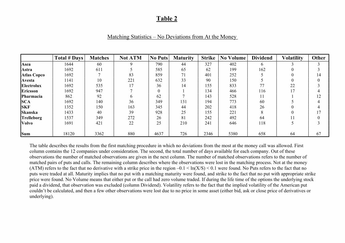
Table 2

Matching Statistics – No Deviations from At the Money

Total # Days Matches Not ATM No Puts Maturity Strike No Volume Dividend Volatility OtherAsea 1644 60 9 790 44 327 402 6 3 3Astra 1692 611 5 585 65 62 199 162 0 3Atlas Copco 1692 7 83 859 71 401 252 5 0 14Avesta 1141 10 221 632 33 90 150 5 0 0Electrolux 1692 535 17 36 14 155 833 77 22 3Ericsson 1692 947 7 0 1 134 466 116 17 4Pharmacia 862 92 6 62 7 143 528 11 1 12SCA 1692 140 36 349 131 194 773 60 5 4SKF 1352 150 163 345 44 202 418 26 0 4Skanska 1433 40 39 928 25 155 221 8 0 17Trelleborg 1537 349 272 26 81 242 492 64 11 0Volvo 1691 421 22 25 210 241 646 118 5 3

Sum 18120 3362 880 4637 726 2346 5380 658 64 67

The table describes the results from the first matching procedure in which no deviations from the most at the money call was allowed. Firstcolumn contains the 12 companies under consideration. The second, the total number of days available for each company. Out of theseobservations the number of matched observations are given in the next column. The number of matched observations refers to the number ofmatched pairs of puts and calls. The remaining column describes where the observations were lost in the matching process. Not at the money(ATM) refers to the fact that no derivative with a strike price in the region –0.1 < ln(X/S) < 0.1 were found. No Puts refers to the fact that noputs were traded at all. Maturity implies that no put with a matching maturity were found, and strike to the fact that no put with appropriate strikeprice were found. No Volume means that either put or the call had zero volume traded. If during the life time of the options the underlying stockpaid a dividend, that observation was excluded (column Dividend). Volatility refers to the fact that the implied volatility of the American putcouldn’t be calculated, and then a few other observations were lost due to no price in some asset (either bid, ask or close price of derivatives orunderlying).

Table 3

Matching Statistics – Deviations from At the Money

Total # Days Matches Not ATM No Puts Maturity Strike No Volume Dividend Volatility OtherAsea 1644 99 9 790 44 131 534 15 19 3Astra 1692 726 5 585 65 5 97 191 15 3Atlas Copco 1688 7 83 857 69 292 358 6 2 14Avesta 1141 15 221 632 33 75 160 5 0 0Electrolux 1692 728 17 36 14 64 691 107 32 3Ericsson 1692 1107 7 0 1 71 340 130 31 5Pharmacia 861 149 6 62 7 77 500 32 17 11SCA 1692 211 36 349 131 71 801 74 15 4SKF 1351 225 163 344 44 79 445 37 10 4Skanska 1429 72 39 924 25 92 247 13 0 17Trelleborg 1537 458 272 26 81 140 445 93 22 0Volvo 1691 559 22 25 210 68 603 182 19 3

Sum 18110 4356 880 4630 724 1165 5221 885 182 80

As table 2 except that it describes the second matching procedure in which deviations from the stock options most at the money is allowed.

Table 4Descriptive Statistics (Averages)

Stock Price TTM Calendar TTM Trading Moneyness EEP EEP/StockP (%) EEP/PutP (%)Asea 501 50 36 0,000 0,64 0,143 3,799Astra 413 57 40 0,006 0,66 0,142 4,068Atlas Copco 249 56 40 0,015 0,27 0,112 3,131Avesta 55 50 36 0,001 0,05 0,085 1,254Electrolux 269 54 38 0,004 0,37 0,152 3,338Ericsson 351 57 40 0,005 0,50 0,144 3,133Pharmacia 140 58 40 -0,003 0,19 0,066 2,993SCA 188 61 42 -0,008 0,35 0,176 3,727SKF 110 54 39 0,002 0,16 0,145 2,825Skanska 163 62 43 0,000 0,16 0,104 1,679Trelleborg 111 54 38 0,002 0,16 0,133 2,577Volvo 396 56 39 0,007 0,50 0,143 3,387

Average 245 56 39 0,003 0,334 0,129 2,99

CallPrice

Spread Call(%)

VolumeCall

OI Call IV Call Put Price Spread Put(%)

Volume Put OI Put IV Put

Asea 21,0 7,55 94 876 0,22 15,5 9,98 41 389 0,24Astra 22,1 3,03 665 10618 0,27 13,5 7,01 226 3265 0,28Atlas Copco 15,8 12,89 87 285 0,28 8,6 14,27 117 234 0,32Avesta 3,8 16,42 326 3665 0,41 3,4 23,05 112 331 0,43Electrolux 14,8 5,14 241 3176 0,29 10,7 9,42 97 863 0,31Ericsson 23,1 2,97 788 7789 0,35 15,5 7,38 254 2036 0,35Pharmacia 8,5 8,87 146 3264 0,35 6,6 19,21 125 820 0,31SCA 8,4 8,79 171 2636 0,27 8,6 15,39 71 610 0,29SKF 6,6 7,33 215 3036 0,33 5,1 11,85 94 785 0,35Skanska 10,8 7,66 118 2832 0,35 9,1 11,99 47 362 0,37Trelleborg 7,4 6,02 328 4237 0,43 5,9 12,24 88 863 0,44Volvo 22,2 4,21 393 3759 0,29 14,7 9,01 139 1356 0,30

Average 13,7 7,6 298 3848 0,32 9,8 12,57 118 993 0,33

The tables gives the average values of each of the companies included in the study. The top table gives the average stock price, time to maturity (TTM) in calendar days and intrading days, the moneyness defined as ln(S/K). The early exercise price (EEP) and EEP in relation to the stock price as well as the put price in %. The next table gives the averagestatistic for both calls and puts. The average price, the average mid spread of the derivative prices in %, volume of derivative, open interest (OI) and finally, the average impliedvolatility (IV).

Table 5

Descriptive Statistics –Shorting Abolishment

Panel i): Whole Sample

First Observ. Last Observ. Min Max Average Std #A : No Shorting 1988-02-01 1991-11-21 -0,0322 0,0237 -0,0007 0,0031 1453

C : No Restriction 1992-02-06 1994-10-21 -0,0452 0,0731 -0,0004 0,0037 2691

Panel ii): Long Stock – Pos. Dev.

Average Median Std #A + 0,0070 0,0059 0,0066 20

C + 0,0051 0,0019 0,0121 101

Panel iii): Short Stock – Neg. Dev.

Average Median Std #A – -0,0053 -0,0037 0,0052 228

C – -0,0041 -0,0022 0,0057 425

In the table the data has been divided into two periods A and C, the first corresponding to the short constrained period and the second to theperiod without a constraint. The interim period 1991-11-22 to 1992-02-05 has been deleted since, even though it was allowed, virtually no onelended and borrowed during this period for tax reasons. Furthermore, positive deviations from PCP, corresponding to the case when one goeslong the stock, and negative deviations from PCP, corresponding to the case when one goes long the stock, has been separated in panel ii) andiii). The data has been aggregated over all firms where deviations from PCP have been normalised by the strike price.

Table 6

Testing Shorting Abolishment

A + > C + A – < C –Differences in means 0,69 (0,244) 2,68 (0,003)**

Differences in medians 2,72 (0,003)** 3,95 (0)***

Test the differences between the period A, the short restricted period, and C, during which norestriction on shorting existed. The data are aggregated across firms and normalised by thestrike price. Positive and negative deviations from PCP are considered separately, whileobservations that comply with PCP are not included. Finally, the interim period 1991-11-22 to1992-02-05 is excluded for tax reasons. The tests concerns the mean and median. The nullhypothesis is that there is no difference between the periods. The alternative one sidedhypothesis is that the positive deviations in period A is larger than those in period C and thatthe negative deviations in period A are more negative than those in period C. Differences inmedians are tested using Wilcoxon’s test, means using a t-test (since the degrees of freedomhere is very large it is assumed that the normal distribution could be used instead of the tdistribution). The numbers in the tables are the test statistics and the numbers withinparenthesis the p-values. */**/*** indicates significance levels at 5%/1% and 0,1% level.

Table 7

Testing Shorting Abolishment - Regression

Panel i)

IndependentVariable

Coefficient Standard Deviation P-value

VolumeU 1,19E-11 7,39E-11 0,872VolumeD 4,81E-07 1,01E-06 0,636Std/P 0,0707 0,0482 0,146Intercept 0,0019 0,0021 0,346Dummy 0,0024 0,0028 0,1894

Panel ii)

IndependentVariable

Coefficient Standard Deviation P-value

VolumeU 1,57E-11 1,99E-11 0,43VolumeD -2,31E-08 4,42E-07 0,958Std/P -0,0296 0,00860 0,0010**Intercept -0,0030 0,00045 0***Dummy -0,0012 0,00046 0,0045**

In the above table the following regression has been performed:

tttttt PStdVolumeDVolumeUD εββββα +++++=∆ /1 4321

where ∆ denotes the deviations from put call parity (PCP). In panel i) only positive deviations fromPCP are used as dependent variable and in panel ii) only negative deviations are considered. D denotesa dummy that takes on the value 1 during the short constrained period and 0 when no restriction apply.VolumeU is the daily volume of the underlying stock and VolumeD is the average daily volume of theput and the call. Std/P is the standard deviation of the underlying stock calculated on a monthly basiswith non-overlapping observations. Furthermore, the measure has been standardised with the averageunderlying stock price over the same period. For all variables but the dummy the two tailed p-value isgiven. For the dummy the one sided p-value for the alternative hypothesis that it is significantly greaterthan zero in panel i) and significantly lower than zero in panel ii).

Table 8

Descriptive Statistics –The Introduction of Futures

Panel i): Whole Sample

First Observ. Last Observ. Min Max Average Std #A : No Shorting 1988-02-01 1991-11-21 -0,0322 0,0237 -0,0007 0,0031 1453

B : No Futures 1992-02-06 1993-02-12 -0,0131 0,0731 -0,0004 0,0066 368

D : No Restriction 1992-07-01 1994-10-21 -0,0452 0,0446 -0,0005 0,0030 2323

Panel ii): Long Stock – Pos. Dev.

Average Median Std #A + 0,0070 0,0059 0,0066 20

B + 0,0106 0,0022 0,0220 24

D + 0,0034 0,0016 0,0057 77

Panel iii): Short Stock – Neg. Dev.

Average Median Std #A – -0,0053 -0,0037 0,0052 228

B – -0,0034 -0,0026 0,0027 118

D – -0,0043 -0,0020 0,0065 307

In the table the data has been divided into three periods A, B and D. A corresponding to the short constrained period, B to the period during lending andborrowing of stocks were allowed but no futures on individual stocks were traded. D is the period when there are no shorting restrictions and futures onindividual stocks were traded. The interim period 1991-11-22 to 1992-02-05 has also been deleted since, even though it was allowed, virtually no one lendedand borrowed during this period for tax reasons. Furthermore, positive deviations from PCP in panel ii), corresponding to the case when one goes long thestock, and negative deviations from PCP in panel iii), corresponding to the case when one goes long the stock, has been separated. Finally, the data has beenaggregated over all firms. All the deviations from PCP have been normalised by the strike price.

Table 9

Testing the Introduction of Futures

Panel i): Long Stock – Pos. Dev.

A + > B + B + > D + A + > D +Differences in means -0,69 (0,757) 2,63 (0,004)** 2,45 (0,007)**

Differences in medians 1,57 (0,057) 0,98 (0,163) 2,88 (0,001)**

Panel ii): Short Stock – Neg. Dev.

A – < B – B – < D – A – < D –Differences in means 3,61 (0)*** -1,41 (0,921) 1,87 (0,03)*

Differences in medians 2,26 (0,011)* 1,7 (0,043)* 4 (0)***

As table 6 except that it describes the testing of differences between the periods A, short restricted period, and B, period when shorting wasallowed but when futures were not traded, as well as between B and D, period during which shorting is allowed and futures on individual stocksare traded. Also differences between period A and D are tested for.

Table 10

Testing the Introduction of Futures - Regression

Panel i)

IndependentVariable

Coefficient Standard Deviation P-value

VolumeU 5,59E-07 9,70E-07 0,57VolumeD 1,18E-11 7,07E-11 0,87Std/P 0,1163 0,0479 0,017*Intercept -0,0021 0,0023 0,35D1 0,0049 0,0028 0,036*D2 0,0095 0,0027 0,0002***

Panel ii)

IndependentVariable

Coefficient Standard Deviation P-value

VolumeU 1,77E-11 2,01E-11 0,38VolumeD -5,93E-08 4,44E-07 0,89Std/P -0,0282 0,0088 0,0010**Intercept -0,0032 0,0005 0***D1 -0,0010 0,0005 0,017*D2 0,0005 0,0006 0,808

Panel iii)

Variable Coefficient P-valueFrom panel i): D1-D2 -0,0046 1From panel ii): D2-D1 0,0016 0***

In the above table in panels i) and ii) the following regression has been performed:ttttttt PStdVolumeDVolumeUDD εβββββα ++++++=∆ /21 54321

D2 is dummy which is 1 during the period when shorting is allowed but no futures weretraded. In all remaining periods it is 0. The p-value is given for the one sided alternativehypothesis that D2 is larger than zero in panel i) and smaller than zero in panel ii). All othervariables are the same as in table 7. In panel iii) differences between the two dummies are tested for. In the first row a sided testthat D1>D2 from panel i) is considered while the second row tests that D2>D1 from panel ii).

Table 11

Foreign Trade

Stockholm’s share in % Type of UnderlyingAsea 24,3 A - REAstra 25,0 A - REEricsson 25,6 B - UNVolvo 29,1 B - RETrelleborg 36,6 B - REAtlas Copco 36,8 A - UNElectrolux 39,9 B - UNSKF 42,0 B - UNSCA 66,2 B - REPharmacia 73,3 B - REAvesta 1 RESkanska 1 B - RE

Second column gives the turn over at Stockholm Stock Exchange in relation to the total turnover at London, Nasdaq and Stockholm for the unrestricted share, company wise. The thirdcolumn gives the type of underlying share for the stock option. RE denotes restricted type ofshares which couldn’t be traded abroad, and UN denotes the unrestricted type that could. Aand B indicates vote power, A shares having more votes than B shares.

Table 12

Company by Company test

AverageA-C(neg)

AverageA-C (pos)

MedianA-C(neg)

MedianA-C (pos)

Total - Total+

Type ofUnderlying

Skanska -0,0152 - -0,0169 - 9 1 B - RESCA -0,0051 - -0,0050 - 33 1 B - RETrelleborg -0,0023 -0,0335 -0,0040 -0,0487 65 9 B - REEricsson -0,0023 0,0005 -0,0003 0,0031 159 36 B - UNPharmacia -0,0069 -0,0087 -0,0069 -0,0024 2 10 B - REAstra -0,0019 - -0,0025 - 133 32 A - REVolvo -0,0011 - -0,0013 - 64 17 B - REElectrolux 0,0010 0,0217 0,0001 0,0220 113 11 B - UNSKF 0,0022 - 0,0025 - 53 3 B - UNAsea - - - - 19 1 A - REAtlas Copco - - - - 1 0 A - UNAvesta - - - - 2 0 RE

Sum 653 121

Second column contains the average negative deviation sin period A minus the averagenegative deviations in period C. Column three is the same but for positive deviations, and incolumns four and five the same thing has been calculated for the median. For companies thatlack deviations in a certain direction no estimate is given. The total number of negative andpositive deviations for each company is given in columns six and seven. The last columncontains the type of underlying.

Table 13

Descriptive Statistics – Foreign Trade

Panel i) – Unrestricted Shares:

Long Stock – Pos. Dev.

Average Median Std #A + 0,0077 0,0058 0,0077 11C + 0,0047 0,0019 0,0078 39

Short Stock – Neg. Dev.

Average Median Std #A – -0,0044 -0,0027 0,0053 127C – -0,0042 -0,0025 0,0060 198

Panel i) – Restricted Shares:

Long Stock – Pos. Dev.

Average Median Std #A + 0,0063 0,0073 0,0054 9C + 0,0054 0,0017 0,0142 62

Short Stock – Neg. Dev.

Average Median Std #A – -0,0064 -0,0057 0,0049 101C – -0,0039 -0,0021 0,0054 227

In the table the data has been divided into two periods A and C, the first corresponding to the short constrained period and the second to theperiod without a constraint. The interim period 1991-11-22 to 1992-02-05 has been deleted. Furthermore, only deviations from PCP areconsidered. In panel i) only firms with stock options that have unrestricted shares as underlying, which are tradable abroad, are considered.While panel ii) consider stock options with an underlying stock that is not tradable abroad. Otherwise exactly as in table 5.

Table 14

Testing the Effects of Foreign Trade

Panel i) - Unrestricted Group:

A + > C + A – < C –Differences in means 1,12 (0,13) 0,19 (0,422)

Differences in medians 1,86 (0,031)* 0,66 (0,252)

Panel ii) - Restricted Group:

A + > C + A – < C –Differences in means 0,18 (0,426) 4,04 (0)***

Differences in medians 1,74 (0,04)* 5,15 (0)***

The same tests as in table 6 are performed, with the difference that the data sample isdivided into two groups. The first group is based on stock options with unrestrictedunderlying shares which are tradable abroad, panel i), while second is based restrictedshares which are not tradable abroad, panel ii).