GBIO0002-1 Bioinformatics

and Genetics

(Previous GBIO0009-1 Bioinformatics)

Introductory lecture Databases and R statistical language

Instructors • Course instructors

– Prof. Kristel Van Steen

• Office: 0/15 in B37

• E-mail: kristel.VanSteen@ulg.ac.be

• http://www.montefiore.ulg.ac.be/~kvansteen

– Prof. Franck DEQUIEDT

• Office: level +5, B34 (GIGA tower)

• E-mail: fdequiedt@ulg.ac.be

• Teacher Assistant

– Kyrylo Bessonov

• Office: 1/16 in B37

• kbessonov@ulg.ac.be

Course Scope This course is introduction to

bioinformatics and genetics fields

covering wide array of topics:

• accessing and working with main

biological DB (PubMed, Ensembl);

• sequence alignments;

• statistical genetics;

• microarray/genotype data analysis

• gene regulation mechanisms

• basic Molecular Biology concepts

Bioinformatics

Definition: the collection, classification,

storage, and analysis of biochemical

and biological information using

computers especially as applied to

molecular genetics and genomics

(Merriam-Webster dictionary)

Definition: a field that works on the

problems involving intersection of

Biology/Computer Science/Statistics

Genetics Definition: Study of heredity in general and

of genes in particular

(Concise Encyclopedia)

1.In 19th century Gregor Mendel formulated the basic concepts

of heredity

2.In 1909s Wilhelm Johannsen introduced a new word - gene

3.In 1909s Thomas Hunt Morgan provided evidence that genes

occur on chromosomes and that adjacent

4.In 1940s Oswald Avery showed that DNA is the chromosome

component that carries genetic information.

5.In 1962s the molecular structure of DNA was deduced by

James D. Watson, Francis Crick, and Maurice Wilkins.

6.In 1970s development of genetic recombination techniques

Course expected outcomes

• Gain a taste of various bioinformatics

fields coupled to hands-on knowledge

• Be able to perform

– multiple sequence alignments

– query biological databases

programmatically

– perform basic GWAS and microarray

analysis

– present scientific papers

Course practical aspects

• Mode of delivery: in class

• Activities:

– reading of scientific literature

– practical assignments (programming in R)

– in-class group presentations

• Meeting times:

– Thursdays from 2pm-6pm

– Room 1.123, Montefiore Institute (B28)

Course practical aspects

• Course material: will be posted on

Prof. Kristel Van Steen (lectures) and/or

Kyrylo Bessonov’s (practicals) website(s)

• Assignment submission: will be

done online via a special submission

website

– After the deadline, the assignment should be

e-mailed to Kyrylo Bessonov

(kbessonov@ulg.ac.be)

What will we be doing?

• We’ll cover a selected recent topics

in bioinformatics and genetics both

trough lectures and assignments

(including student’s presentations)

– reading papers from the bioinformatics

literature and analyzing/critiquing them

– Self-learning through assignments

– In-class hands-on presentation of tools

How will we do it?

• “Theory” classes

– All course notes are in English.

– Instructors

• Kristel Van Steen

• Franck DEQUIEDT

• The “theory” part of the course is

meant to be interactive:

– In-class discussions of papers / topics

How will we do it?

• “Practical” classes • During these classes will be looking at practical

aspects of the topics introduced in theory classes. It

is suggested to execute sample R scripts and

demonstrations on your PCs.

• Optional reading assignments will be assigned:

– to prepare for discussions in class based on the previously

posted papers (no grading; yet participation grades)

• “Homework assignments” are of 3 types (graded)

– Homework assignments result in a “group” report and

can be handed in electronically in French or in English

– Homework assignments constitute an important part of this

course

Types of HW assignments • Three types of homework assignments are:

– Literature style assignment (Type 1)

• A group of students is asked to select a paper

from the provided ones. The group prepares in-

class presentation and a written report

• All oral presentations of HW1,HW2, HW3 will be

done at the end of the semester (all together)

– Programming style assignment (Type 2)

• A group is asked to develop an R code to

answer assignment questions

– Classical style assignment (Type 3)

• A group is provided with questions to be

answered in the written report. Usually R scripts

are provided and require execution / modification

Report writing tips

• Every homework assignment involves writing a

short report

– Suggested length approximately five single-spaced

typed pages of text, excluding figures, tables and

bibliography

– Longer reports are accetable

• It should contain

– an abstract (e.g., brief description of the paper content,

description of the problem)

– results/discussion part

– If citations are made to other papers, there should be a

bibliography (any style is OK)!

• Only one report per group is needed.

• Submit report via online system

Course materials

• All course materials will be either

posted on Prof. Kristel van Steen’s

and/or Kyrylo Bessonov’s websites.

– Please check both sites

• There is no course book

• Final course schedule will be posted

online shortly

Evaluation scheme

• Written exam: 40% of the final mark

– Multiple choice questions/open book

– In French / English

• Assignments: 50% of the final mark

– Total of 3 assignments

• Participation in discussions (10%)

– Throughout the course

– During oral student’s presentations

• Last lecture of the course

Assignment Submission Step by Step Guide

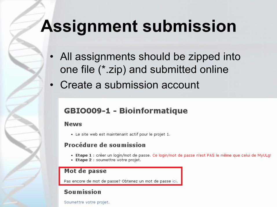
Assignment submission

• All assignments should be zipped into

one file (*.zip) and submitted online

• Create a submission account

Account creation • Any member of the group can submit assignment

• Account details will be emailed to you automatically

• All GBIO009-1 students should create an account

Submit your assignment • After account creation login into a submission page

• The remaining time to deadline is displayed. Good idea to

check it from time to time in order to be on top of things

• File extension should be zip

• Can submit assignment as many times as you wish

Introduction to A basic tutorial

Definition

• “R is a free software environment for

statistical computing and graphics”1

• R is considered to be one of the most

widely used languges amongst

statisticians, data miners,

bioinformaticians and others.

• R is free implementation of S language

• Other commercial statistical packages

are SPSS, SAS, MatLab

1 R Core Team, R: A Language and Environment for Statistical Computing, Vienna, Austria (http://www.R-project.org/)

Why to learn R?

• Since it is free and open-source, R is

widely used by bioinformaticians and

statisticians

• It is multiplatform and free

• Has wide very wide selection of

additional libraries that allow it to use

in many domains including

bioinformatics

• Main library repositories CRAN and

BioConductor

Programming? Should I be scared?

• R is a scripting language and, as

such, is much more easier to learn

than other compiled languages as C

• R has reasonably well written

documentation (vignettes)

• Syntax in R is simple and intuitive if

one has basic statistics skills

• R scripts will be provided and

explained in-class

Topics covered in this tutorial

• Operators / Variables

• Main objects types

• Plotting and plot modification functions

• Writing and reading data to/from files

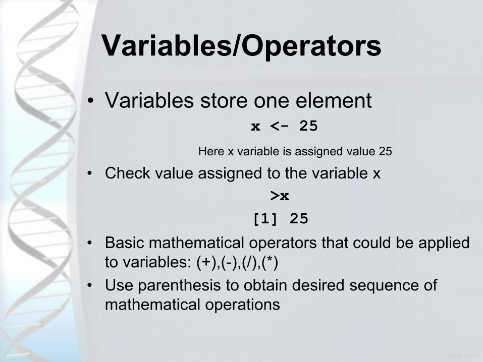
Variables/Operators

• Variables store one element x <- 25

Here x variable is assigned value 25

• Check value assigned to the variable x

>x

[1] 25

• Basic mathematical operators that could be applied

to variables: (+),(-),(/),(*)

• Use parenthesis to obtain desired sequence of

mathematical operations

Arithmetic operators

• What is the value of small z here? >x <- 25

> y <- 15

> z <- (x + y)*2

> Z <- z*z

> z

[1] 80

Vectors

• Vectors have only 1 dimension and

represent enumerated sequence of

data. They can also store variables > v1 <- c(1, 2, 3, 4, 5)

> mean(v1)

[1] 3

The elements of a vector are specified

/modified with braces (e.g. [number]) > v1[1] <- 48

> v1

[1] 48 2 3 4 5

Logical operators

• These operators mostly work on

vectors, matrices and other data types

• Type of data is not important, the same

operators are used for numeric and

character data types Operator Description

< less than

<= less than or equal to

> greater than

>= greater than or equal to == exactly equal to != not equal to

!x Not x x | y x OR y

x & y x AND y

Logical operators

• Can be applied to vectors in the

following way. The return value is

either True or False > v1

[1] 48 2 3 4 5

> v1 <= 3

[1] FALSE TRUE TRUE FALSE FALSE

R workspace

• Display all workplace objects

(variables, vectors, etc.) via ls(): >ls()

[1] "Z" "v1" "x" "y" "z"

• Useful tip: to save “workplace” and

restore from a file use: >save.image(file = " workplace.rda")

>load(file = "workplace.rda")

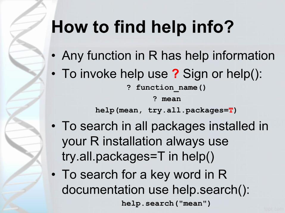
How to find help info?

• Any function in R has help information

• To invoke help use ? Sign or help(): ? function_name()

? mean

help(mean, try.all.packages=T)

• To search in all packages installed in

your R installation always use

try.all.packages=T in help()

• To search for a key word in R

documentation use help.search(): help.search("mean")

Basic data types

• Data could be of 3 basic data types:

– numeric

– character

– logical

• Numeric variable type: > x <- 1

> mode(x)

[1] "numeric"

Basic data types

• Logical variable type (True/False): > y <- 3<4

> mode(y)

[1] "logical"

• Character variable type: > z <- "Hello class"

> mode(z)

[1] "character"

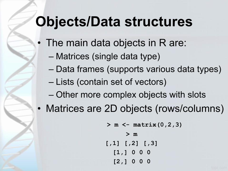
Objects/Data structures

• The main data objects in R are:

– Matrices (single data type)

– Data frames (supports various data types)

– Lists (contain set of vectors)

– Other more complex objects with slots

• Matrices are 2D objects (rows/columns)

> m <- matrix(0,2,3)

> m

[,1] [,2] [,3]

[1,] 0 0 0

[2,] 0 0 0

Lists

• Lists contain various vectors. Each

vector in the list can be accessed by

double braces [[number]] > x <- c(1, 2, 3, 4)

> y <- c(2, 3, 4)

> L1 <- list(x, y)

> L1

[[1]]

[1] 1 2 3 4

[[2]]

[1] 2 3 4

Data frames

• Data frames are similar to matrices but

can contain various data types > x <- c(1,5,10)

> y <- c("A", "B", "C")

> z <-data.frame(x,y)

x y

1 1 A

2 5 B

3 10 C

• To get/change column and row names

use colnames() and rownames()

Factors

• Factors type are similar to character

vectors but can provide info on

– on unique variables in the vector

– variable counts (quantity) > letters = c("A","B","C","A","C","C")

> letters = factor(letters)

[1] A B C A C C

Levels: A B C

> summary(letters)

A B C

2 1 3

Input/Output

• To read data into R from a text file use read.table()

– read help(read.table) to learn more

– scan() is a more flexible alternative raw_data <-read.table(file="data_file.txt")

• To write data into R from a text file use

read.table() > write.table(mydata, "data_file.txt")

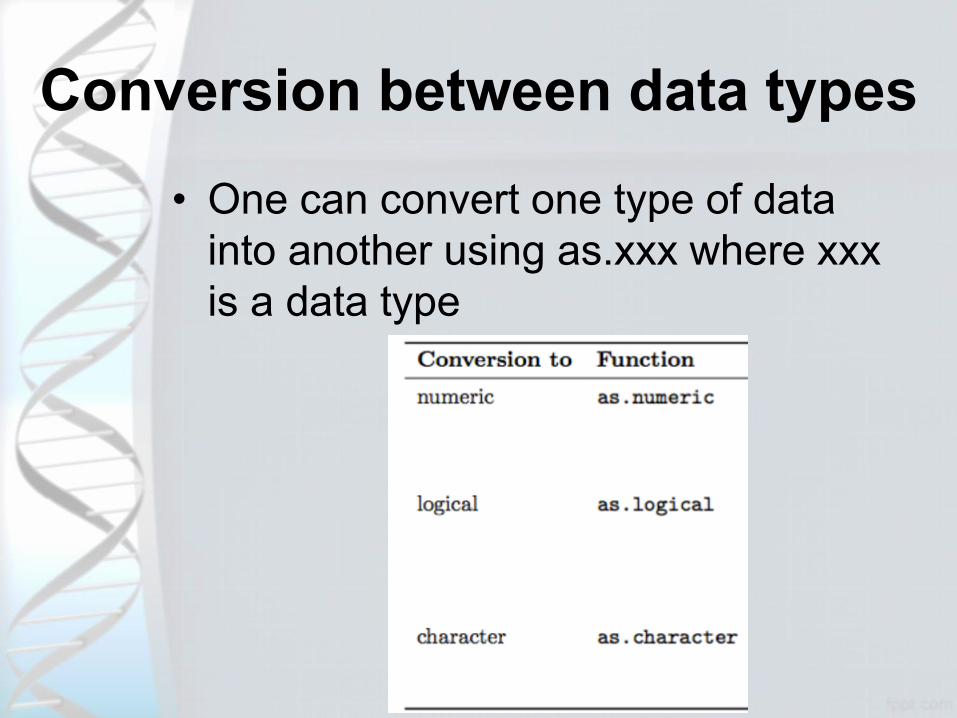
Conversion between data types

• One can convert one type of data

into another using as.xxx where xxx

is a data type

Plots generation in R

• R provides very rich set of plotting

possibilities

• The basic command is plot()

• Each library has its own version of plot() function

• When R plots graphics it opens

“graphical device” that could be

either a window or a file

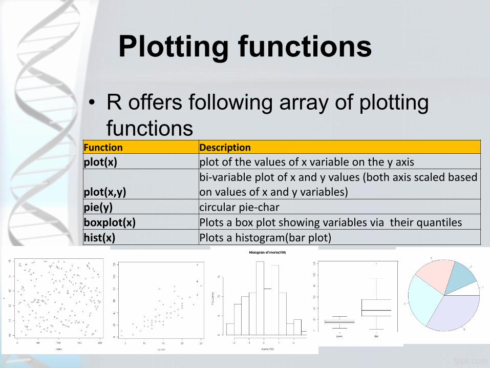
Plotting functions

• R offers following array of plotting

functions Function Description

plot(x) plot of the values of x variable on the y axis

plot(x,y) bi-variable plot of x and y values (both axis scaled based on values of x and y variables)

pie(y) circular pie-char boxplot(x) Plots a box plot showing variables via their quantiles hist(x) Plots a histogram(bar plot)

Plot modification functions

• Often R plots are not optimal and one

would like to add colors or to correct

position of the legend or do other

appropriate modifications

• R has an array of graphical parameters

that are a bit complex to learn at first

glance. Consult here the full list

• Some of the graphical parameters can be specified inside plot() or using other

graphical functions such as lines()

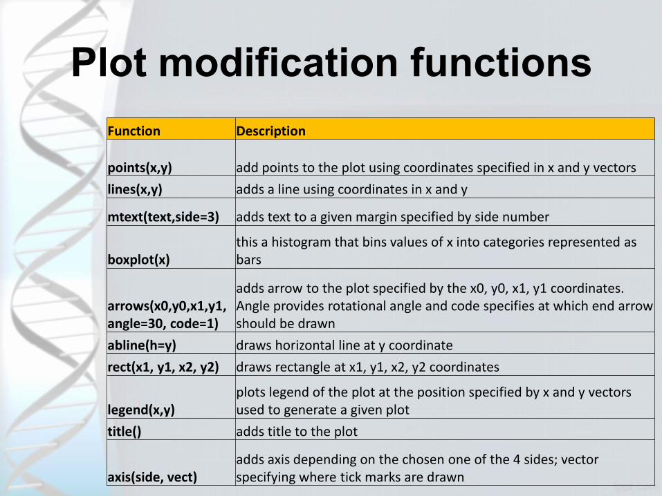
Plot modification functions

Function Description

points(x,y) add points to the plot using coordinates specified in x and y vectors

lines(x,y) adds a line using coordinates in x and y

mtext(text,side=3) adds text to a given margin specified by side number

boxplot(x) this a histogram that bins values of x into categories represented as bars

arrows(x0,y0,x1,y1, angle=30, code=1)

adds arrow to the plot specified by the x0, y0, x1, y1 coordinates. Angle provides rotational angle and code specifies at which end arrow should be drawn

abline(h=y) draws horizontal line at y coordinate

rect(x1, y1, x2, y2) draws rectangle at x1, y1, x2, y2 coordinates

legend(x,y) plots legend of the plot at the position specified by x and y vectors used to generate a given plot

title() adds title to the plot

axis(side, vect) adds axis depending on the chosen one of the 4 sides; vector specifying where tick marks are drawn

Demos

• R functionality demonstration

– Plots: demo(graphics)

– 3D: demo(persp)

– GLM data modelling: demo(lm.glm)

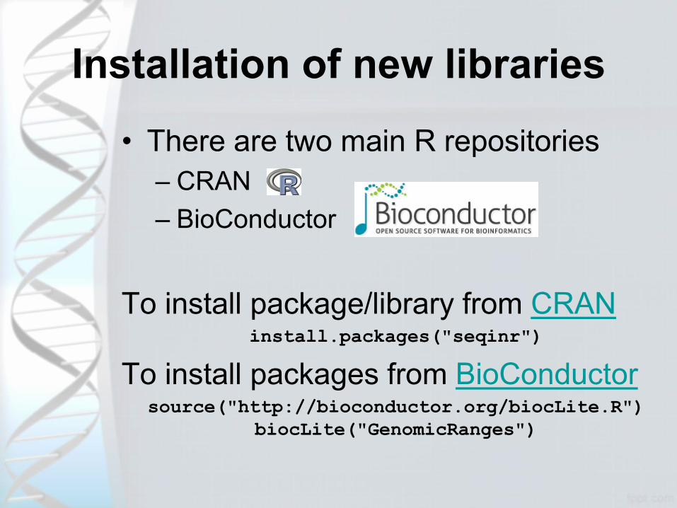
Installation of new libraries

• There are two main R repositories

– CRAN

– BioConductor

To install package/library from CRAN install.packages("seqinr")

To install packages from BioConductor source("http://bioconductor.org/biocLite.R")

biocLite("GenomicRanges")

Installation of key libraries

• Install latest R version on your PC. Go

to http://cran.r-project.org/

• Install following libraries by running install.packages(c("seqinr", "muscle", "ape",

"GenABEL")

source("http://bioconductor.org/biocLite.R")

biocLite("limma","affy","hgu133plus2.db","Biosti

ngs")

Conclusions

• We hope this course will provide you

with the good array of analytical and

practical skills

• We chose R for this course as it is very

flexible language with large scope of

applications and is widely used

What are we looking for?

Data & databases

Biologists Collect LOTS of Data • Hundreds of thousands of species to explore

• Millions of written articles in scientific journals

• Detailed genetic information:

• gene names

• phenotype of mutants

• location of genes/mutations on chromosomes

• linkage (distances between genes)

• High Throughput lab technologies

• PCR

• Rapid inexpensive DNA sequencing (Illumina HiSeq)

• Microarrays (Affymetrix)

• Genome-wide SNP chips / SNP arrays (Illumina)

• Must store data such that

• Minimum data quality is checked

• Well annotated according to standards

• Made available to wide public to foster research

What is database?

• Organized collection of data

• Information is stored in "records“, "fields“, “tables”

• Fields are categories

– Must contain data of the same type (e.g. columns

below)

• Records contain data that is related to one object

(e.g. protein, SNP) (e.g. rows below)

SNP ID SNPSeqID Gene +primer -primer

D1Mit160_1 10.MMHAP67FLD1.seq lymphocyte antigen 84 AAGGTAAAAGGCAAT

CAGCACAGCC

TCAACCTGGAGTCAGA

GGCT

M-05554_1 12.MMHAP31FLD3.seq procollagen, type III,

alpha

TGCGCAGAAGCTGA

AGTCTA

TTTTGAGGTGTTAATGG

TTCT

Genome sequencing

generates lots of data

Biological Databases The number of databases is contantly growing!

- OBRC: Online Bioinformatics Resources Collection

currently lists over 2826 databases (2013)

Main databases by category Literature

• PubMed: scientific & medical abstracts/citations

Health

• OMIM: online mendelian inheritance in man

Nucleotide Sequences

• Nucleotide: DNA and RNA sequences

Genomes

• Genome: genome sequencing projects by organism

• dbSNP: short genetic variations

Genes

• Protein: protein sequences

• UniProt: protein sequences and related information

Chemicals

• PubChem Compound: chemical information with structures,

information and links

Pathways

• BioSystems: molecular pathways with links to genes, proteins

• KEGG Pathway: information on main biological pathways

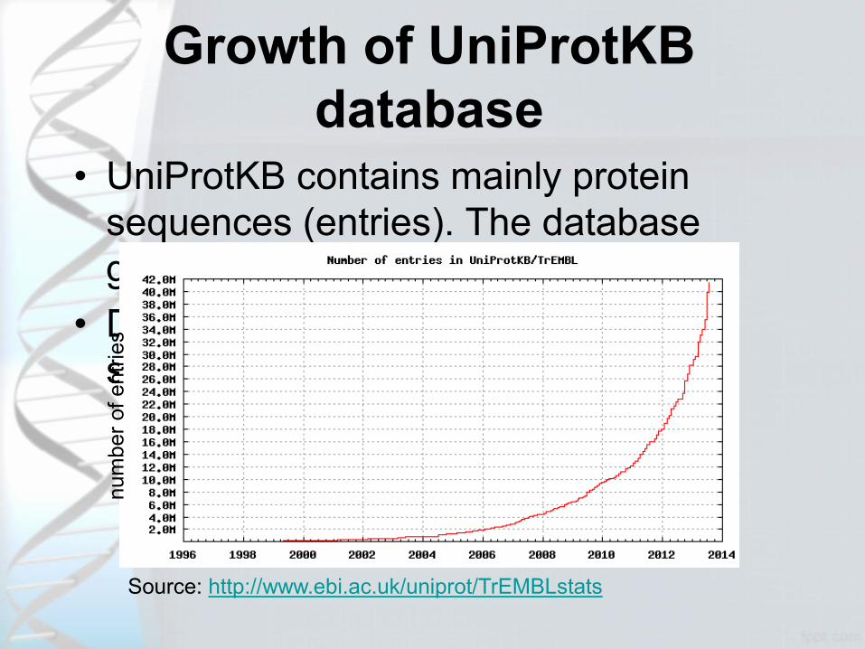
Growth of UniProtKB

database • UniProtKB contains mainly protein

sequences (entries). The database

growth is exponential

• Data management issues? (e.g.

storage, search, indexing?)

Source: http://www.ebi.ac.uk/uniprot/TrEMBLstats

num

ber

of

entr

ies

Primary and Secondary

Databases

Primary databases

REAL EXPERIMENTAL DATA (raw)

Biomolecular sequences or structures and associated

annotation information (organism, function, mutation linked to

disease, functional/structural patterns, bibliographic etc.)

Secondary databases

DERIVED INFORMATION (analyzed and annotated)

Fruits of analyses of primary data in the primary sources (patterns, blocks, profiles etc. which represent the most conserved

features of multiple alignments)

Primary Databases

Sequence Information – DNA: EMBL, Genbank, DDBJ

– Protein: SwissProt, TREMBL, PIR, OWL

Genome Information – GDB, MGD, ACeDB

Structure Information – PDB, NDB, CCDB/CSD

Secondary Databases

Sequence-related Information – ProSite, Enzyme, REBase

Genome-related Information – OMIM, TransFac

Structure-related Information – DSSP, HSSP, FSSP, PDBFinder

Pathway Information – KEGG, Pathways

GenBank database

• Contains all DNA and protein sequences described in the scientific literature or collected in publicly funded research

• One can search by protein name to get DNA/mRNA sequences

• The search results could be filtered by species and other parameters

GenBank main fields

NCBI Databases contain more

than just

DNA & protein sequences

NCBI main portal: http://www.ncbi.nlm.nih.gov/

Fasta format to store sequences

Saccharomyces cerevisiae strain YC81 actin (ACT1) gene

GenBank: JQ288018.1

>gi|380876362|gb|JQ288018.1| Saccharomyces cerevisiae strain YC81 actin (ACT1)

gene, partial cds

TGGCATCATACCTTCTACAACGAATTGAGAGTTGCCCCAGAAGAACACCCTGTTCTTTTG

ACTGAAGCTCCAATGAACCCTAAATCAAACAGAGAAAAGATGACTCAAATTATGTTTGAA

ACTTTCAACGTTCCAGCCTTCTACGTTTCCATCCAAGCCGTTTTGTCCTTGTACTCTTCC

GGTAGAACTACTGGTATTGTTTTGGATTCCGGTGATGGTGTTACTCACGTCGTTCCAATT

TACGCTGGTTTCTCTCTACCTCACGCCATTTTGAGAATCGATTTGGCCGGTAGAGATTTG

ACTGACTACTTGATGAAGATCTTGAGTGAACGTGGTTACTCTTTCTCCACCACTGCTGAA

AGAGAAATTGTCCGTGACATCAAGGAAAAACTATGTTACGTCGCCTTGGACTTCGAGCA

AGAAATGCAAACCGCTGCTCAATCTTCTTCAATTGAAAAATCCTACGAACTTCCAGATGG

TCAAGTCATCACTATTGGTAAC

•

• The FASTA format is now universal for all

databases and software that handles DNA and

protein sequences

• Specifications: • One header line

• starts with > with a ends with [return]

OMIM database • Online Mendelian Inheritance in Man (OMIM)

• ”information on all known mendelian disorders linked to

over 12,000 genes”

• “Started at 1960s by Dr. Victor A. McKusick as a catalog of

mendelian traits and disorders”

• Linked disease data

• Links disease phenotypes and causative genes

• Used by physicians and geneticists

OMIM – basic search

• Online Tutorial: http://www.openhelix.com/OMIM

• Each search results entry has *, +, # or % symbol

• # entries are the most informative as molecular basis of

phenotype – genotype association is known is known

• Will do search on: Ankylosing spondylitis (AS)

• AS characterized by chronic inflammation of spine

OMIM-search results

• Look for the entires that link to the genes.

Apply filters if needed

Filter results if known SNP is associated to

the entry

Some of the interesting entries. Try to look

for the ones with # sign

OMIM-entries

OMIM Gene ID -entries

OMIM-Finding disease linked genes • Read the report and find genes linked

phenotype (e.g. IL23R)

• Mapping – how the disease gene was found

PubMed database • PubMed is one of the best known

database in the whole scientific

community

• Most of biology related literature from all

the related fields are being indexed by this

database

• It has very powerful mechanism of

constructing search queries

• Many search fields ● Logical operatiors

(AND, OR)

• Provides electronic links to most journals

• Example of searching by author articles

published within 2012-2013

In-class assignment/demo

on

Biological Databases

Demo/Assignment

• Question 1

– Explore OMIM database and key

clinical information on

• glioblastoma (brain cancer)

• Question 2

– Look for literature in PUBMED related

to the disease

• Learn on how to create search queries

Thanks for attention!

Have a nice week!