Gaussian Process Implicit Surfaces

Oliver Williams Andrew FitzgibbonMicrosoft Research, Cambridge, UK

Many applications in computer vision and computer graphics require thedefinition of curves and surfaces. Implicit surfaces [7] are a popular choicefor this because they are smooth, can be appropriately constrained by knowngeometry, and require no special treatment for topology changes. Given a scalarfunction f : Rd 7→ R, one can define a manifold S of dimension d− 1 whereverf(x) passes through a certain value (e.g., 0)

S0 , x ∈ Rd|f(x) = 0. (1)

In this paper we introduce Gaussian processes (GPs) to this area by derivinga covariance function equivalent to the thin plate spline regularizer [2] in whichsmoothness of a function f(x) is encouraged by the energy

E(f) =∫

Ω

(∇T∇f(x)

)2dx (2)

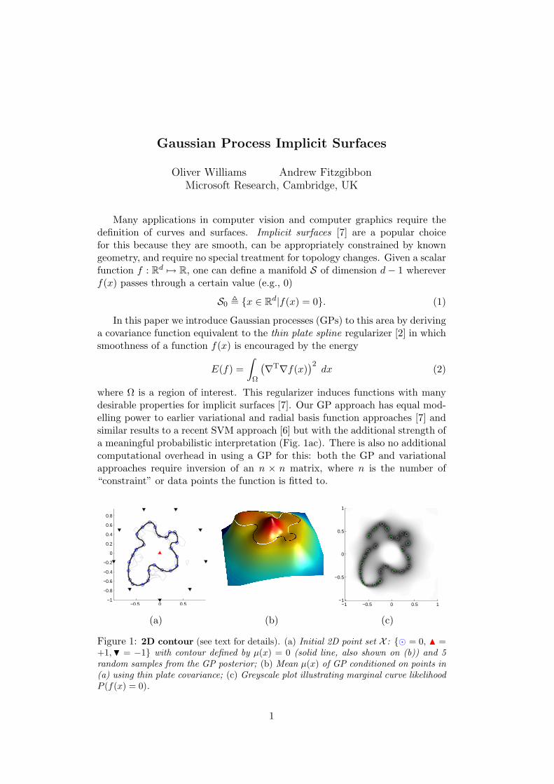
where Ω is a region of interest. This regularizer induces functions with manydesirable properties for implicit surfaces [7]. Our GP approach has equal mod-elling power to earlier variational and radial basis function approaches [7] andsimilar results to a recent SVM approach [6] but with the additional strength ofa meaningful probabilistic interpretation (Fig. 1ac). There is also no additionalcomputational overhead in using a GP for this: both the GP and variationalapproaches require inversion of an n × n matrix, where n is the number of“constraint” or data points the function is fitted to.

−0.5 0 0.5−1

−0.8

−0.6

−0.4

−0.2

0

0.2

0.4

0.6

0.8

−1 −0.5 0 0.5 1−1

−0.5

0

0.5

1

(a) (b) (c)

Figure 1: 2D contour (see text for details). (a) Initial 2D point set X : = 0, N =+1,H = −1 with contour defined by µ(x) = 0 (solid line, also shown on (b)) and 5random samples from the GP posterior; (b) Mean µ(x) of GP conditioned on points in(a) using thin plate covariance; (c) Greyscale plot illustrating marginal curve likelihoodP (f(x) = 0).

1

1 Spline regularization is a Gaussian process

For clarity, we consider the 1D problem in this section; the generalization to2D and 3D is demonstrated below. It is known that a regularizer of the formin equation (2) can be thought of as a Gaussian process prior (see e.g., [3]). Toshow this, we consider the energy as a probability and define D as the lineardifferential operator

E(f) = − log P (f) + const =∫

Ω

(D2f(x)

)2dx. (3)

Using f(Ω) to denote the vector of function values for all points in the regionof interest, the prior may be written (ignoring the constant) as follows:

− log P (f(Ω)) = f(Ω)T[D2]TD2f(Ω), (4)

which corresponds to a multivariate Gaussian distribution with zero mean andcovariance C =

([D2]TD2

)−1 =(D4

)−1.

1.1 The covariance function

We now identify the covariance function c(u, v) giving the entries of C withoutrecourse to online matrix inversion. Rewriting D4C = I reveals c(u, v) to bethe Green’s function of the fourth derivative operator [8]∫

ΩD4(u, w)c(w, v) dw = δ(u− v) ⇒ ∂4

∂r4c(r) = δ(r) (5)

where r , u− v to impose stationarity on the covariance. The solution of thisis

c(r) = 16 |r|

3 + a3r3 + a2r

2 + a1r + a0. (6)

Any odd-powered polynomial terms must be equal to zero in order for thecovariance function to be symmetric (i.e., a3 = a1 = 0). The other requirementis that c be positive semi-definite (psd) [5] and this may be used to set theconstants a0, a2. Since the cubic term will “overpower” the other terms asr →∞, this is not possible for all r ∈ R (psd functions tend to zero at infinity[2]). However, if we restrict ourselves to the domain Ω ⊂ R, it is possible to seta2, a0 such that the covariance tends to zero at its perimeter: if R is the largestmagnitude of r within Ω, stipulating that c(R) = 0 and ∂

∂r c(R) = 0 gives thethin plate covariance

c(r) = 112

(2|r|3 − 3Rr2 + R3

). (7)

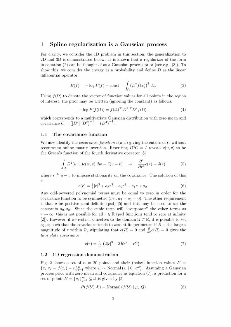
1.2 1D regression demonstration

Fig. 2 shows a set of n = 20 points and their (noisy) function values X ≡xi, ti = f(xi) + εin

i=1 where εi ∼ Normal(εi | 0, σ2

). Assuming a Gaussian

process prior with zero mean and covariance as equation (7), a prediction for aset of points U = ujm

j=1 ⊆ Ω is given by [5]

P (f(U)|X ) = Normal (f(U) | µ, Q) (8)

2

−2 −1 0 1 2−2

−1

0

1

2

−2 −1 0 1 2−2

−1

0

1

2

−1 −0.5 0 0.5 1−1

−0.5

0

0.5

1

(a) (b) (c)

Figure 2: Thin plate vs. squared exponential covariance. (a) Mean (solid line)and 3 s.d. error bars (filled region) for GP regression with covariance given by equation(7); (b) Prediction with covariance function c(ui, uj) = e−α‖ui−uj‖2 with α = 2 (dashedline), 10 (solid) and 100 (dotted); error bars correspond to α = 10; (c) Curve/likelihoodobtained for points of Fig. 1 using squared exponential covariance (“best” α = 8 settingshown).

where

µ = CTux(Cxx + σ2I)−1t and Q = Cuu − CT

ux(Cxx + σ2I)−1Cux. (9)

The matrices are formed by evaluating c(·, ·) between sets of points: i.e., Cxx =[c(xi, xj)], Cux = [c(ui, xj)], and Cuu = [c(ui, uj)].

Fig. 2a shows the mean function and 3 standard deviation error bars forthis data set when Ω = [−2, 2] and σ2 = 0.01 (sd(ui) =

√Qii). Observe how

the mean attempts to minimize the second derivative as dictated by equation(2). In comparison, Fig. 2b shows the predictions if the squared exponential[5] covariance function is employed: the mean interpolant is smooth, but the“compactness” of this covariance leads the mean function to tend towards theGP mean (here zero) away from the data. This will cause undesirable geomet-ric effects in higher dimensions (Fig. 2c). This covariance also suffers from anuisance length-scale parameter (although it does offer smoothness control notavailable with our thin plate covariance).

2 2D curves, 3D surfaces

In order to model 2D curves, given some known points on the curve, we will findf(x) as in equation (1) with d = 2. The training data comprise xi, ti pairswith ti = 0 for points on the curve, plus additional points at ±1 as illustratedin Fig. 1a. The equivalent of equation (5) in Rd is(

∇T∇)2

c(r) = δ(r) (10)

where now c(u, v) = c(r) with r , ‖u− v‖. Solutions to this (with constraintsat the boundary of Ω similar to those in 1D) are given by

2D c(r) = 2r2 log |r| − (1 + 2 log(R))r2 + R2 (11a)

3D c(r) = 2|r|3 + 3Rr2 + R3 (11b)

3

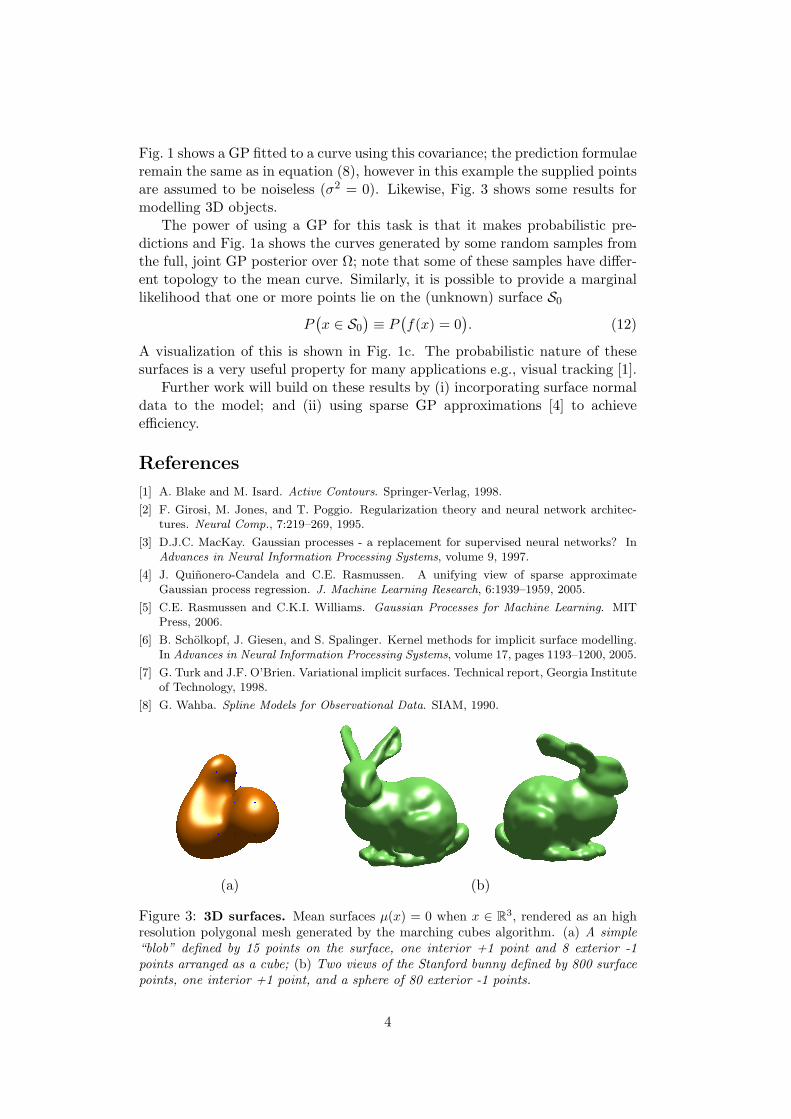
Fig. 1 shows a GP fitted to a curve using this covariance; the prediction formulaeremain the same as in equation (8), however in this example the supplied pointsare assumed to be noiseless (σ2 = 0). Likewise, Fig. 3 shows some results formodelling 3D objects.

The power of using a GP for this task is that it makes probabilistic pre-dictions and Fig. 1a shows the curves generated by some random samples fromthe full, joint GP posterior over Ω; note that some of these samples have differ-ent topology to the mean curve. Similarly, it is possible to provide a marginallikelihood that one or more points lie on the (unknown) surface S0

P(x ∈ S0

)≡ P

(f(x) = 0

). (12)

A visualization of this is shown in Fig. 1c. The probabilistic nature of thesesurfaces is a very useful property for many applications e.g., visual tracking [1].

Further work will build on these results by (i) incorporating surface normaldata to the model; and (ii) using sparse GP approximations [4] to achieveefficiency.

References

[1] A. Blake and M. Isard. Active Contours. Springer-Verlag, 1998.

[2] F. Girosi, M. Jones, and T. Poggio. Regularization theory and neural network architec-tures. Neural Comp., 7:219–269, 1995.

[3] D.J.C. MacKay. Gaussian processes - a replacement for supervised neural networks? InAdvances in Neural Information Processing Systems, volume 9, 1997.

[4] J. Quinonero-Candela and C.E. Rasmussen. A unifying view of sparse approximateGaussian process regression. J. Machine Learning Research, 6:1939–1959, 2005.

[5] C.E. Rasmussen and C.K.I. Williams. Gaussian Processes for Machine Learning. MITPress, 2006.

[6] B. Scholkopf, J. Giesen, and S. Spalinger. Kernel methods for implicit surface modelling.In Advances in Neural Information Processing Systems, volume 17, pages 1193–1200, 2005.

[7] G. Turk and J.F. O’Brien. Variational implicit surfaces. Technical report, Georgia Instituteof Technology, 1998.

[8] G. Wahba. Spline Models for Observational Data. SIAM, 1990.

(a) (b)

Figure 3: 3D surfaces. Mean surfaces µ(x) = 0 when x ∈ R3, rendered as an highresolution polygonal mesh generated by the marching cubes algorithm. (a) A simple“blob” defined by 15 points on the surface, one interior +1 point and 8 exterior -1points arranged as a cube; (b) Two views of the Stanford bunny defined by 800 surfacepoints, one interior +1 point, and a sphere of 80 exterior -1 points.

4