gaussian process implicit surfaces -
TRANSCRIPT
Implicit surface modelling Spline regularization as a Gaussian process GPIS for 2D curves GPIS for 3D surfaces Summary
Gaussian Process Implicit Surfaces
Oliver Williams1
Microsoft Research and Trinity HallCambridge, UK
Gaussian Processes in PracticeBletchley Park, 13 June 2006
1Joint work with Andrew Fitzgibbon

Implicit surface modelling Spline regularization as a Gaussian process GPIS for 2D curves GPIS for 3D surfaces Summary
Talk outline
Implicit surface modelling
Spline regularization as a Gaussian processCovariance function1D regression demonstration
GPIS for 2D curvesCovariance in 2DProbabilistic interpretation
GPIS for 3D surfacesCovariance function
Summary
Implicit surface modelling Spline regularization as a Gaussian process GPIS for 2D curves GPIS for 3D surfaces Summary
Implicit surface
Scalar function f (x) defins a surface wherever it passes through agiven value (e.g., 0)
S0 , x ∈ Rd |f (x) = 0.
Example: Function f (x) for x ∈ R2 defines a closed curve
Implicit surface modelling Spline regularization as a Gaussian process GPIS for 2D curves GPIS for 3D surfaces Summary
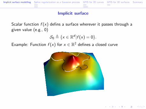
Implicit surface
Scalar function f (x) defins a surface wherever it passes through agiven value (e.g., 0)
S0 , x ∈ Rd |f (x) = 0.Example: Function f (x) for x ∈ R2 defines a closed curve
Implicit surface modelling Spline regularization as a Gaussian process GPIS for 2D curves GPIS for 3D surfaces Summary
Fitting to data points
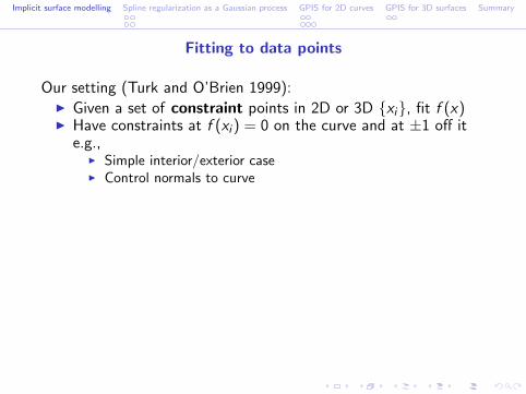
Our setting (Turk and O’Brien 1999):I Given a set of constraint points in 2D or 3D xi, fit f (x)I Have constraints at f (xi ) = 0 on the curve and at ±1 off it
e.g.,I Simple interior/exterior caseI Control normals to curve

Implicit surface modelling Spline regularization as a Gaussian process GPIS for 2D curves GPIS for 3D surfaces Summary
Fitting to data points
Our setting (Turk and O’Brien 1999):I Given a set of constraint points in 2D or 3D xi, fit f (x)I Have constraints at f (xi ) = 0 on the curve and at ±1 off it
e.g.,I Simple interior/exterior caseI Control normals to curve
−0.5 0 0.5−1
−0.5
0
0.5

Implicit surface modelling Spline regularization as a Gaussian process GPIS for 2D curves GPIS for 3D surfaces Summary
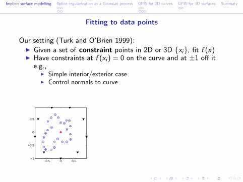
Fitting to data points
Our setting (Turk and O’Brien 1999):I Given a set of constraint points in 2D or 3D xi, fit f (x)I Have constraints at f (xi ) = 0 on the curve and at ±1 off it
e.g.,I Simple interior/exterior caseI Control normals to curve
−0.5 0 0.5−1
−0.5
0
0.5Alternative method: parametric surface:x(t), y(t), [z(t)]
I What t to assign to data points?
I How to handle different topologies?
I Can represent non-closedcurves/surfaces
Implicit surface modelling Spline regularization as a Gaussian process GPIS for 2D curves GPIS for 3D surfaces Summary
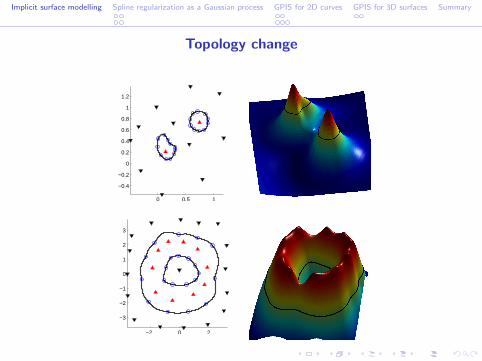
Topology change
0 0.5 1
−0.4
−0.2
0
0.2
0.4
0.6
0.8
1
1.2
−2 0 2
−3
−2
−1
0
1
2
3

Implicit surface modelling Spline regularization as a Gaussian process GPIS for 2D curves GPIS for 3D surfaces Summary
Regularization
Find function passing through constraint points which minimizesthin-plate spline energy
E (f ) =
∫Ω
(∇T∇f (x)
)2dx
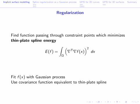
Fit f (x) with Gaussian processUse covariance function equivalent to thin-plate spline

Implicit surface modelling Spline regularization as a Gaussian process GPIS for 2D curves GPIS for 3D surfaces Summary
Regularization
Find function passing through constraint points which minimizesthin-plate spline energy
E (f ) =
∫Ω
(∇T∇f (x)
)2dx
Fit f (x) with Gaussian process
Use covariance function equivalent to thin-plate spline
Implicit surface modelling Spline regularization as a Gaussian process GPIS for 2D curves GPIS for 3D surfaces Summary
Regularization
Find function passing through constraint points which minimizesthin-plate spline energy
E (f ) =
∫Ω
(∇T∇f (x)
)2dx
Fit f (x) with Gaussian processUse covariance function equivalent to thin-plate spline
Implicit surface modelling Spline regularization as a Gaussian process GPIS for 2D curves GPIS for 3D surfaces Summary
Gaussian distribution
I Follow derivation in (MacKay 2003) in 1D
I consider the energy as a probability and define D as the lineardifferential operator
E (f ) = − log P(f ) + const =
∫Ω
(D2f (x)
)2dx .
I Use f (Ω) as vector of function values for all points in Ω:
− log P(f (Ω)) = f (Ω)T[D2]TD2f (Ω),
I This is a Gaussian disribution with mean zero and covariance:
C =([D2]TD2
)−1=
(D4
)−1.

Implicit surface modelling Spline regularization as a Gaussian process GPIS for 2D curves GPIS for 3D surfaces Summary
Covariance function
I Entries of C indexed by u, v ∈ Ω∫Ω
D4(u,w)c(w , v) dw = δ(u − v) ⇒ ∂4
∂r4c(r) = δ(r)
where we impose stationarity with r = u − v .
I Interpret as spectral density and solve
F[c(r)
](ω) = ω−4
⇒ c(r) = 16 |r |
3 + a3r3 + a2r
2 + a1r + a0.
Implicit surface modelling Spline regularization as a Gaussian process GPIS for 2D curves GPIS for 3D surfaces Summary
Covariance function
c(r) = 16 |r |
3 + a3r3 + a2r
2 + a1r + a0
Find constants using constraints on c(·)I Symmetry: a3 = a1 = 0
I Postive definiteness: simulate by making c(r) → 0 at ∂Ω
c(r) = 112
(2|r |3 − 3Rr2 + R3
).
where R is the largest magnitude of r within Ω.

Implicit surface modelling Spline regularization as a Gaussian process GPIS for 2D curves GPIS for 3D surfaces Summary
1D regression demonstration
GP predicts function values for set of points U ⊆ Ω
P(f (U)|X ) = Normal (f (U) | µ, Q)
where
µ = CTux(Cxx + σ2I )−1t and Q = Cuu − CT
ux(Cxx + σ2I )−1Cux .
The matrices are formed by evaluating c(·, ·) between sets ofpoints: i.e., Cxx = [c(xi , xj)], Cux = [c(ui , xj)], andCuu = [c(ui , uj)].

Implicit surface modelling Spline regularization as a Gaussian process GPIS for 2D curves GPIS for 3D surfaces Summary
1D regression demonstration
−2 −1 0 1 2−2
−1
0
1
2
−2 −1 0 1 2−2
−1
0
1
2
(a) (b)
Figure: Thin plate vs. squared exponential covariance. Mean (solid
line) and 3 s.d. error bars (filled region) for GP regression (a) Thin-
plate covariance; (b) Squared exponential covariance function c(ui , uj) =
e−α‖ui−uj‖2
with α = 2, 10 and 100; error bars correspond to α = 10.
Implicit surface modelling Spline regularization as a Gaussian process GPIS for 2D curves GPIS for 3D surfaces Summary
Covariance in 2D
I In 2D the Green’s equation is(∇T∇
)2c(r) = δ(r)
where now c(u, v) = c(r) with r , ‖u − v‖.
I Solution (with similar constraints at the boundary of Ω)
c(r) = 2r2 log |r | −(1 + 2 log(R)
)r2 + R2
Implicit surface modelling Spline regularization as a Gaussian process GPIS for 2D curves GPIS for 3D surfaces Summary
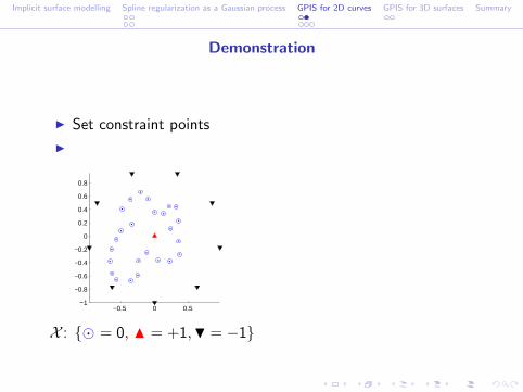
Demonstration
I Set constraint points
I
−0.5 0 0.5−1
−0.8
−0.6
−0.4
−0.2
0
0.2
0.4
0.6
0.8
X : = 0, N = +1,H = −1
Implicit surface modelling Spline regularization as a Gaussian process GPIS for 2D curves GPIS for 3D surfaces Summary
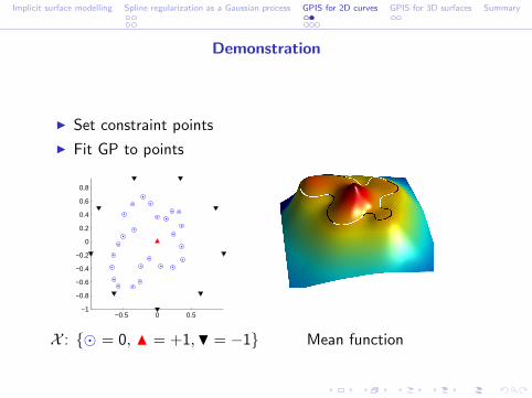
Demonstration
I Set constraint points
I Fit GP to points
−0.5 0 0.5−1
−0.8
−0.6
−0.4
−0.2
0
0.2
0.4
0.6
0.8
X : = 0, N = +1,H = −1 Mean function
Implicit surface modelling Spline regularization as a Gaussian process GPIS for 2D curves GPIS for 3D surfaces Summary
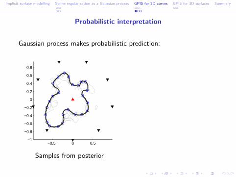
Probabilistic interpretation
Gaussian process makes probabilistic prediction:
−0.5 0 0.5−1
−0.8
−0.6
−0.4
−0.2
0
0.2
0.4
0.6
0.8
Samples from posterior
Implicit surface modelling Spline regularization as a Gaussian process GPIS for 2D curves GPIS for 3D surfaces Summary
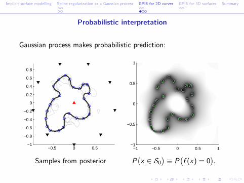
Probabilistic interpretation
Gaussian process makes probabilistic prediction:
−0.5 0 0.5−1
−0.8
−0.6
−0.4
−0.2
0
0.2
0.4
0.6
0.8
−1 −0.5 0 0.5 1−1
−0.5
0
0.5
1
Samples from posterior P(x ∈ S0
)≡ P
(f (x) = 0
).
Implicit surface modelling Spline regularization as a Gaussian process GPIS for 2D curves GPIS for 3D surfaces Summary
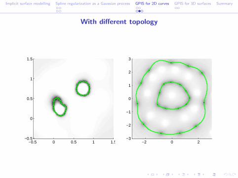
With different topology
−0.5 0 0.5 1 1.5−0.5
0
0.5
1
1.5
−2 0 2−3
−2
−1
0
1
2
3
Implicit surface modelling Spline regularization as a Gaussian process GPIS for 2D curves GPIS for 3D surfaces Summary
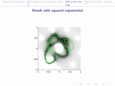
Result with squared exponential
−1 −0.5 0 0.5 1−1
−0.5
0
0.5
1
Implicit surface modelling Spline regularization as a Gaussian process GPIS for 2D curves GPIS for 3D surfaces Summary
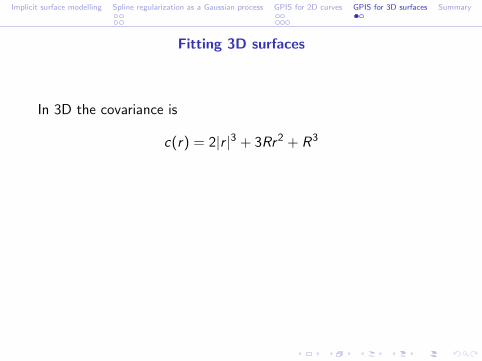
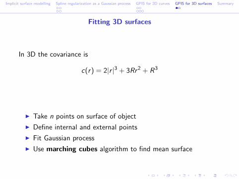
Fitting 3D surfaces
In 3D the covariance is
c(r) = 2|r |3 + 3Rr2 + R3
I Take n points on surface of object
I Define internal and external points
I Fit Gaussian process
I Use marching cubes algorithm to find mean surface

Implicit surface modelling Spline regularization as a Gaussian process GPIS for 2D curves GPIS for 3D surfaces Summary
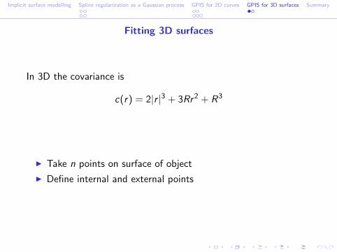
Fitting 3D surfaces
In 3D the covariance is
c(r) = 2|r |3 + 3Rr2 + R3
I Take n points on surface of object
I Define internal and external points
I Fit Gaussian process
I Use marching cubes algorithm to find mean surface
Implicit surface modelling Spline regularization as a Gaussian process GPIS for 2D curves GPIS for 3D surfaces Summary
Fitting 3D surfaces
In 3D the covariance is
c(r) = 2|r |3 + 3Rr2 + R3
I Take n points on surface of object
I Define internal and external points
I Fit Gaussian process
I Use marching cubes algorithm to find mean surface
Implicit surface modelling Spline regularization as a Gaussian process GPIS for 2D curves GPIS for 3D surfaces Summary
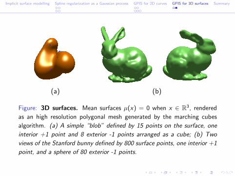
(a) (b)
Figure: 3D surfaces. Mean surfaces µ(x) = 0 when x ∈ R3, rendered
as an high resolution polygonal mesh generated by the marching cubes
algorithm. (a) A simple “blob” defined by 15 points on the surface, one
interior +1 point and 8 exterior -1 points arranged as a cube; (b) Two
views of the Stanford bunny defined by 800 surface points, one interior +1
point, and a sphere of 80 exterior -1 points.

Implicit surface modelling Spline regularization as a Gaussian process GPIS for 2D curves GPIS for 3D surfaces Summary
Summary
I Gaussian processes can be used to define curves and surfaces
I Appropriate covariance must be used to obtain high qualityresults
I By using a GPIS, curves and surfaces have a meaningfulprobabilistic interpretation
Shortcomings / ideas for future work:
I Exploit probabilistic nature of GPIS in computer visionproblems
I More elegant methods for constraining surface normals?
I Can this be used to learn a meaningful prior?
I Scale/smoothness control?