lattice gauge theories - an introduction

Lattice Gauge Theories - An Introduction

Andreas Wipf

Theoretisch-Physikalisches InstitutFriedrich-Schiller-University Jena

Bayrischzell, März 2018

Andreas Wipf (TPI Jena) Lattice Gauge Theories - An Introduction

1 Why lattice field theories

2 Lattice Gauge Theories

3 Observables in lattice gauge theories

4 Fermions on a Lattice


Why discretize quantum field theories 3 / 41

weakly interacting systems :subsystems almost independent of each other

weakly correglated quantum systemsweakly interacting effective dof (quasi particles)quantum electrodynamicsweak interactionweak field gravitystrong interaction at high energies

underlying Gaussian fixed pointperturbations theory applicable


strongly interacting systems:properties explained by strong correlations between subsystems

strongly correlated quantum systemshigh temperature superconductivityultra cold atoms in optical latticesspin systems near phase transitionsstrong field gravitystrong interaction at low energies

underlying interacting fixes pointdependent on scale a theory can be weakly or strongly interactingneeds non-perturbative methods


various approaches 5 / 41

soluble modelslow dimensions:exactly soluble models: Ising-, Schwinger-, Thirring model, . . .high symmetry:conformal symmetry, supersymmetry, integrable systems, dualities,. . .

approximations:mean field, strong coupling expansion, expansions for high/lowtemperataure, phenomenological models, . . .functional methods:∞-system of coupled Schwinger-Dyson equationsfunctional renormalization grouplattice formulation, ab-initio lattice simulationlattice-QFT⇒ particular statistical systempowerful simulation methods of statistical physics


global gauge transformations 6 / 41

Gauge theories in continuum

all fundamental theories = gauge theorieselectrodynamics: abelian U(1) gauge theoryelectroweak model: SU(2)×U(1) gauge theorystrong interaction: SU(3) gauge theorygravity: gauge theory

matter field φ(x) ∈ V, global gauge transform φ(x)→ Ωφ(x)

Ω ∈ G gauge groupinvariant scalar product on V : (Ωφ,Ωφ) = (φ, φ)

invariant Lagrange density

L(φ, ∂µφ) = (∂µφ, ∂µφ)− V (φ)

invariant potential V (Ωφ) = V (φ)


local gauge transformations 7 / 41

construction of locally gauge invariant theory

φ(x) −→ φ′(x) = Ω(x)φ(x), Ω(x) ∈ G

∂µφ wrong transformation property; need covariant derivative

Dµφ = ∂µφ− igAµφ, g coupling constant

needs new dynamical field Aµ ∈ g (g = Lie algebra)requirement: Dµφ transforms as φ does =⇒

D′µ = ΩDµΩ−1 ⇐⇒ A′µ = ΩAµΩ−1 − ig∂µΩΩ−1

field strength

Fµν =ig

[Dµ,Dν ] = ∂µAν − ∂νAµ − ig[Aµ,Aν ] ∈ g


gauge invariant Lagrangian 8 / 41

transforms in adjoint representation

Fµν(x) −→ Ω(x)Fµν(x)Ω−1(x)

L Lorentz invariant, parity invariant, gauge invariant⇒

L = −14

tr FµνFµν +(Dµφ,Dµφ

)− V (φ)

principle of minimal coupling:begin with globally invariant theory, replace ∂µ → Dµadd Yang-Mills term − 1

4 tr FµνFµν (cp. electrodynamics)symmetries and particle content→ Lagrange density (almost)


Parallel transport 9 / 41

Cyx path from x to y , parametrized x(s)

parallel transport of φ along path:

0 = xµDµφ⇐⇒dφ(s)

ds= igAµ(s)xµ(s)φ(s), φ(s) ≡ φ

(x(s)

)cp. time-dependent Schrödinger equationlet x(0) = x and x(1) = y ⇒

φ(y) = P exp

(ig∫ 1

0ds Aµ(s)xµ(s)

)φ(x)

parallel transport along path Cyx

U(Cyx ,A) = P exp

(ig∫Cyx

A

)∈ G, A = Aµdxµ


gauge invariant variables 10 / 41

paths Cyx and Czy can be composed: Czy Cyx = Czx

U(Czy Cyx ,A) = U(Czy ,A)U(Cyx ,A)

exists (useless?) nonabelian Stokes theoremgauge transformation

U(Cyx ,A′) = Ω(y) U(Cyx ,A) Ω−1(x)

from x to y parallel transportet field

U(Cyx )φ(x) transforms as φ(y)

gauge invariant objects (over-complete)

tr U(Cxx ) holonomies(φ(y),U(Cyx )φ(x)

)scalar products


Lattice field theories (Euclidean) 11 / 41

field theory in continuous spacetime Rd ill-defined (UV-divergences)spacetime continuum→ discretize spacetimee.g. hypercubic lattice Λ with lattice constant alattice sites, lattice links, lattice plaquettes, lattice cubes, . . .minimal momentum p = 2π/a⇒ theory regularized in UVmatter field φ(x)→ φx , x ∈ Λ lattice fieldderivative→ difference oparator or lattice derivative, e.g.

(∂µφ)x =1aφ(x + aeµ)− φ(x)

gauge theory: covariant lattice derivative

(Dµφ)x ≡1aφx+aeµ

− Ux,µφx


gauge invariant matter action 12 / 41

Ux,µ parallel transporter from x to x + aeµlattice action for matter field (a = 1)

Smatter =∑x,µ

(Dµφx ,Dµφx

)+∑

x

V (φx )

= −2<∑x,µ

(φx+eµ

Ux,µφx)

+∑

x

(2d(φx , φx

)+ V (φx

)

IR cutofffinite lattice Λ = Z

4 → Nt × N3

needed in simulationsextrapolate to N →∞

classical spin systemnearest neighbour interactionSmatter real, positivelocally gauge invariant

x1

x2

t

1

N

1

N


gauge invariant gauge action 13 / 41

new dynamical compact field Ux,µ ∈ Gparallel transporter along link from x to x + aeµreplaces dynamical noncompact field Aµ(x) ∈ g

relation via parallel transport

Aµ smooth on scale a⇒

Ux,µ ≈ eig aAµ(x) = 1+ ig aAµ(x) + . . .

covariant derivative

(Dµφ)x =1aφx+aeµ −

(1+ ig aAµ(x) + . . .

)φx

= (∂µφ)x − ig(Aµφ)x + O(a)

there are O(a2) improved lattice derivative


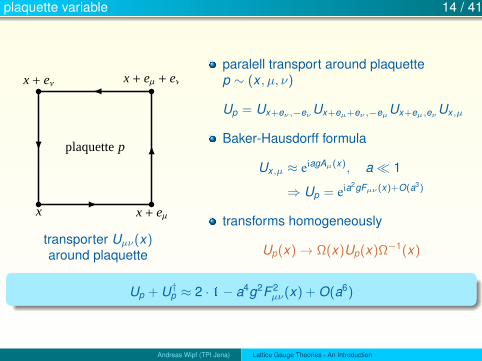
plaquette variable 14 / 41

x x + eµ

x + eµ + eνx + eν

plaquette p

transporter Uµν(x)around plaquette

paralell transport around plaquettep ∼ (x , µ, ν)

Up = Ux+eν ,−eνUx+eµ+eν ,−eµ

Ux+eµ,eνUx,µ

Baker-Hausdorff formula

Ux,µ ≈ eiagAµ(x), a 1

⇒ Up = eia2gFµν(x)+O(a3)

transforms homogeneously

Up(x)→ Ω(x)Up(x)Ω−1(x)

Up + U†p ≈ 2 · 1− a4g2F 2µν(x) + O(a6)


Yang-Mills theory on lattice 15 / 41

lattice action for gauge field configuration U = Ux,µ

SW(U) =1

g2N

∑p

tr1− 1

2

(Up + U†p

)(Wilson) .

in particular for G = SU(2)

SW =1

2g2

∑p

tr (1− Up)

improved lattice action (Symanzik)

SYM − SSy = O(a2)

⇒ faster convergence to continuum limit a→ 0


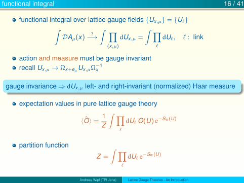
functional integral 16 / 41

functional integral over lattice gauge fields Ux,µ = U`∫DAµ(x)

?−→∫ ∏

(x,µ)

dUx,µ =

∫ ∏`

dU`, ` : link

action and measure must be gauge invariantrecall Ux,µ → Ωx+eµ

Ux,µΩ−1x

gauge invariance⇒ dUx,µ left- and right-invariant (normalized) Haar measure

expectation values in pure lattice gauge theory

〈O〉 =1Z

∫ ∏`

dU` O(U) e−SW(U)

partition function

Z =

∫ ∏`

dU` e−SW(U)


invariant integration 17 / 41

consider irreducible representations U → R(U) of compact G, dim=dRPeter-Weyl theorem: The functions R(U)ab form an orthogonal basison L2(dU), and

(Rab,R′cd) ≡ ∫ Rab(U)R′cd (U) dU =

δRR′

dRδacδbd ,

Lemma: The characters χR(U) = trR(U) form a ON-basis of invariantfunctions, f (U) = f (ΩUΩ−1) in L2(dU), such that

(χR, χR′

)= δRR′

identities

orthogonality:(R ab, χR′

)=(χR′ ,R ab) =

δRR′

dRδab

gluing:∫

dΩχR(UΩ−1)χR′ (ΩV ) =δRR′

dRχR(UV )

cutting:∫

dΩχR(ΩUΩ−1V ) =1

dRχR(U)χR(V )

decomposition of unity:∑R

dR χR(U) = δ(1,U)


the curse of dimensionality 18 / 41

functional integral on finite d-dimensional lattice

dV dim(G)− dimensional integral

SU(2) gauge theory, moderate hyper-cubic 164-lattice⇒

786 432− dimensional integral

cannot be calculated numerically!stochastic methods

generate many configurationsdistributed according to e−action

method of important samplingMonte Carlo (MC) algorithms (Metropolis, Heat bath, . . . )with ferminions: expensive (hybrid MC + . . . )


observables in pure lattice gauge theories 19 / 41

only gauge invariant observables (Elitzur theorem)traces of parallel transporters along loops

W [C] = tr (U`n · · ·U`1 ) , C = `n · · · `1 Wilson loops

W [R,T ] rectangular loop, edge lengths R, Tstatic energy of a static qq-pair separated by R

Vqq(R) = − limT→∞

1T

log〈W [R,T ]〉

string tension and Lüscher term

Vqq(R) ∼ σR + const.− cR

+ o(R−1)

T

R


static quarks in representation R 20 / 41

confinement⇒ σ > 0⇒ W ∼ exp(−σRT ) area law (strong coupling)only colorless (gauge invariant) states are seen

Click here

−6

−4

−2

0

2

4

6

8

0.0 0.5 1.0 1.5 2.0 2.5

VR/µ

µR

R = 7R = 14R = 27R = 64R = 77R = 77′R = 182R = 189

linear potentials for static quarks in different G2 representations


string-breaking for static charges in adjoint of SU(N) or for G2 21 / 41

dynamical quarksmeson, diquark qq →2 mesons, diquarks

charges in adjoint or G2

energy scale = 2 mglueball

decay products: glue-lumps

−2

−1

0

1

2

3

4

5

6

7

0 1 2 3 4 5 6

VR/µ

µR

R = 7, β = 30, N = 483R = 14, β = 30, N = 483R = 7, β = 20, N = 323R = 14, β = 20, N = 323


some observables in pure gauge theories 22 / 41

confinement: ⇒ only colorless (gauge invariant) states are seenQCD: confinement at low temperature, no gluonsglueballs = colourless bound states of gluonsstate by acting with interpolating operator on vacuum

|ψ(τ)〉 = O(τ)|0〉, O(τ) = eτ HO(0)e−τ H

two-point function

GE (τ) = 〈0|T O(τ)O(0)|0〉 =∑

n

|〈0|O|n〉|2e−Enτ

asymptotically large Euclidean time

GE (τ) −→ |〈0|O|0〉|2 + |〈0|O|1〉|2e−E1τ(

1 + O(e−τ(E2−E1)

))


excited state with 〈0|O|1〉 6= 0→ asymptoticsO|0〉 and |1〉 should have same quantum numbersparity, angular momentum (cubic group), charge conjugation, . . .glueballs: O combination of paralles transportersmasses of glueballs in MeV MC-simulation of Chen et al.

JPC 0++ 2++ 0−+ 1+− 2−+ 3+−

mG[MeV] 1710 2390 2560 2980 3940 3600

JPC 3++ 1−− 2−− 3−− 2+− 0+−

mG[MeV] 3670 3830 4010 4200 4230 4780


gauge theories at finite temperature 24 / 41

partition function: β-periodic gauge fields

Z (β) =

∮ ∏(x,µ)

dUx,µ e−SW(U)

space

time

Px

Z ⇒ thermodynamic potentials

T < Tc : confinement→ glueballs

T > Tc : deconfinement→ gluon plasma

phase diagram, order of transition(s)

order parameter: Polyakov loop Px


Polyakov loop 25 / 41

center symmetry:non-periodic gauge trafoby center trafoorder parameter:Polyakov loop Px

Px = tr( Nt∏

x0=1

U(x0,x ),0

)

SU(3): center = Z3

broken below Tc

restored above Tc

−0.5 −0.4 −0.3 −0.2 −0.1 0 0.1 0.2 0.3 0.4 0.5

−0.5

−0.4

−0.3

−0.2

−0.1

0

0.1

0.2

0.3

0.4

0.5

0

2000

4000

6000

Im

Re

histogram of Polyakov loop


expected phase diagram of QCD


fermions 27 / 41

fermions on the lattice

functional approach: ψα(x) anticommuting

ψα(x), ψβ(y) = ψα(x), ψβ(y) = ψα(x), ψβ(y) = 0

fermionic integration = multi-dimensional Grassmann integral∫DψDψ · · · ≡

∫ ∏x

∏α

dψα(x) dψα(x) . . .

expectation value of observable A

〈0|A|0〉 =1ZF

∫DψDψ A(ψ, ψ) e−SF(ψ,ψ)

partition function

ZF =

∫DψDψ e−SF


bilinear classical action SF for the fermion field

SF =

∫ddx L(ψ, ψ), L = ψ(x)Dψ(x)

Grassmann integration→ determinant of fermion operator

ZF =

∫DψDψ exp

(−∫

ddx ψ(x)Dψ(x)

)= det D

corresponding formula for complex scalars

ZB =

∫DφDφexp

(−∫

ddx φ(x)Aφ(x)

)=

1det A

Majorana fermions (susy)

ZF =

∫Dψ exp

(−∫

ddx ψ(x)Dψ(x)

)= Paff(D)


fermion determinant 29 / 41

expectation values in full lattice gauge theory

〈(U)〉 =1Z

∫O(U) dµ(U), dµ(U) = det(D) e−S[U]DU, Z =

∫dµ(U)

subtle: first order Dirac operator on latticeon finite lattice D (huge) matrixstochastic methods applicable if det(D) e−S[U] > 0usually: D is γ5-hermitean

γ5Dγ5 = D†

eigenvalues come in complex conjugated pairs⇒ determinant real

P(λ) ≡ det(λ− D) = det γ5(λ− D)γ5 = det(λ− D†

)= P∗(λ∗)


problems with fermions 30 / 41

λ root⇒ λ∗ root, real, not necessarily positivesign problem if det D changes signexample

D = /∂ + m +O γ5 hermitean⇐⇒ ∂µ = −∂†µ, O = O†, [γ5,O] = 0

natural choice (∂µf)

(x) =12

(f (x + eµ)− f (x − eµ))

gauge theories: chiral symmetry for massless fermions

eiαγ5D eiαγ5 = D ⇔ γ5,D = 0

naive Dirac operatorD = γµ∂µ + m

γ5-hermitean, chirally symmetric for m = 0


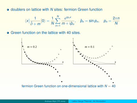
doublers on lattice with N sites: fermion Green function

〈x∣∣ 1∂ + m

∣∣0〉 =1N

N∑n=1

eipnx

m + ipn, pn = sin pn, pn =

2πnN

Green function on the lattice with 40 sites.

x

m = 0.2

x

m = 0.1

fermion Green function on one-dimensional lattice with N = 40


dispsersion relations 32 / 41

p

0 π

p2

p2

p2

dispersion relations for −∂2

p2 : continuum relationp2 from ∂

p2 from nearest neighborLaplacian (∼Wilson operator)

(∆f )(x) =∑

µ(f (x + eµ)− 2f (x) + f (x − eµ))

∂µ ⇒ chiral and γ5−hermitean /∂

doublers in spectrum


Wilson operator 33 / 41

Theorem (Nielsen-Ninomiya)exists no translational invariant D fulfilling

1 locality: D(x − y) . e−γ|x−y|,2 continuum limit: lima→0 D(p) =

∑µ γ

µpµ,

3 no doublers: D(p) is invertible if p 6= 0,4 chirality: γ5,D = 0.

nice topological proofgive up chiral invariance: Wilson fermions

Sw = Snaive −r2

∑x

ψx a∆ψx =∑

x

ψxDwψx ,

Wilson operatorDw = γµ∂µ −

ar2∆


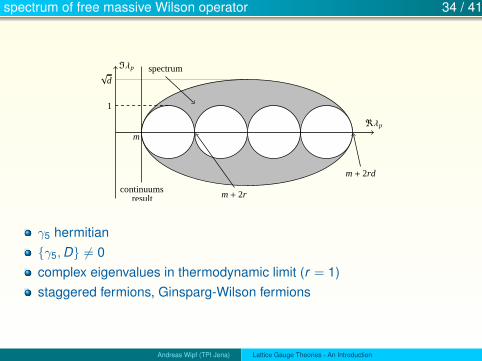
spectrum of free massive Wilson operator 34 / 41

√d

continuums

ℜλp

m + 2rd

m + 2r

ℑλp

m

spectrum

result

1

γ5 hermitianγ5,D 6= 0complex eigenvalues in thermodynamic limit (r = 1)staggered fermions, Ginsparg-Wilson fermions


lattice actionSF =

∑x

ψx (Dwψ)x

gauge invariance: first parallel transport and then compare (r = 1)

(Dw)xy = (m + d)δxy

− 12

∑µ

((1+γµ)Uy,−µδx,y−eµ + (1−γµ)Uy,µδx,y+eµ

)rescaling (Wilson)

ψ → 1√m + d

ψ

gauge invariant action

Sw =∑

x

ψxψx − κ∑x,µ

(ψx−eµ

(1+γµ)Ux,−µψx + ψx+eµ(1−γµ)Ux,µψx

)hopping parameter κ = (2m + 2d)−1


full lattice field theory 36 / 41

lattice functional integrals

Z =

∫ ∏`

dU`∏

x

dψx dψx e−Sg(U)−SF(ψ,ψ)

=

∫ ∏`

dU` det(D[U]) e−Sg(U)

=

∫ ∏`

dU` sign(det D) (det M)1/2 e−Sg(U)

M = D†D ⇒ det M ≥ 0.try stochastic method with

dµ(U) = (det M)1/2 e−Sg(U)DU


pseudo fermions 37 / 41

expectation values

〈O[U]〉 =

∫dµ(U) sign(det D) O(U)∫

dµ(U) sign(det D)

problem with re-weighing: sign(det D) may average to zerofermion determinant: method of pseudofermion fields

(det M)1/2 =

∫ ∏p

Dφ†pDφp e−SPF , SPF =

NPF∑p=1

(φp,M−qφp

)q · NPF = 1/2. If det D > 0⇒

Z =

∫ ∏`

dU`DφDφ∗ e−Sg(U)−SPF(U,φ,φ†)

HMC algorithm: force given by gradient of non-local Sg + SPF


observables depending on femion fields 38 / 41

rHMC dynamics M−q → rational approximation

M−q ≈ α0 +NR∑

r=1

αr

M + βr

fermion correlators: SF quadratic in ψ ⇒Wick contractione.g. interpolating operator for pion

Oπ(t) =∑xψ(t ,x )τγ5ψ(t ,x )

Wick-contraction

〈0|O†π(t)Oπ(0)|0〉 =1Z

∫ ∏`

dU` GFGF det(D[U]) e−Sg(U)

∼ amplitude · e−mπ t

⇒ masses of bound states: mesons, baryons, glueballs, . . .


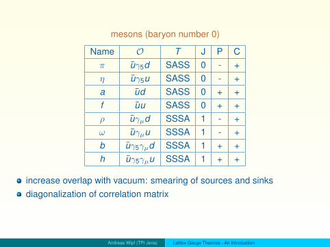
mesons (baryon number 0)

Name O T J P Cπ uγ5d SASS 0 - +η uγ5u SASS 0 - +a ud SASS 0 + +f uu SASS 0 + +ρ uγµd SSSA 1 - +ω uγµu SSSA 1 - +b uγ5γµd SSSA 1 + +h uγ5γµu SSSA 1 + +

increase overlap with vacuum: smearing of sources and sinksdiagonalization of correlation matrix


G2 masses of mesons, diquarks, baryons 40 / 41

heavy ensemble light ensemble

Wellegehausen, Maas, Smekal, AW (2013)


summary, . . . 41 / 41

simulations: stochastic, linear algebra, programmingworks for QCD at T = 0 and T > 0 (fermions β-anti-periodic)but: fermions difficult and expensivethermodynamic and continuum extrapolations: N →∞ and a→ 0realistic quark masses achievedproblem: finite baryon density, det(D) complex⇒ conventional MC does not worksimulations for supersymmetric YM theories

lattice breaks supersymmetrysome results of mass spectrum of N = 1 SYMnew result on N = (2, 2) and N = (8, 8)relevant for AdS/CFT (Gregory-Laflamme instability)

books: Montvay-Münster, Rothe, Lang-Gattringer, AW, . . .


lattice gauge theories - an introduction

Documents