gast-d validation report - federal aviation administration
TRANSCRIPT

FEDERAL AVIATION ADMINISTRATION
GAST-D Validation Report Results from the HI INR Development Contract
3/19/2013
Document includes the objectives, flight test plan, and results from the HI INR GAST-D Avionics Development contract.
1
Contents
1. Introduction ...................................................................................................................................... 2
1.1. Overview ...................................................................................................................................... 2
1.2. Tasks and Schedule ..................................................................................................................... 2
1.3. Report Coverage .......................................................................................................................... 3
2. Flight Testing ..................................................................................................................................... 3
2.1. Test Equipment and Setup .......................................................................................................... 3
2.2. Flight Test Objectives/Profiles ................................................................................................... 4
2.3. Additional Data Collection and Analysis for Task Area II Flight Testing ................................ 5
2.4. Summary of Completed Flight Profiles ...................................................................................... 6
3. Task Area I – GAST C Compliance and Performance ................................................................. 9
4. Task Area II: Implementation of GAST-D Protocols for MOPS Validation ........................... 12
4.1. GAST-D Flight Testing Navigation Sensor Error ..................................................................... 12
4.2. Dual Solution Ionospheric Gradient Monitor (DSIGMA) ........................................................ 14
4.3. Differential Correction Magnitude Check ................................................................................ 17
4.4. Airborne Code Carrier Divergence Filtering ........................................................................... 19
4.5. Fault Detection for Satellite Addition ...................................................................................... 21
4.6. Fault Detection .......................................................................................................................... 21
4.7. Reference Receiver Fault Monitoring (RRFM) ........................................................................ 22
4.8. VDB Message Authentication Protocols .................................................................................. 25
5. Summary & Future Work .............................................................................................................. 26
Appendix I: Final Report on The Development of Airborne Equipment Class (AEC) D Avionics
for the LAAS (Honeywell)……………………………………………………………………………………………………... 27
2
1. Introduction
1.1. Overview
In August 2010, a cost-sharing contract was awarded to Honeywell International to implement GAST-D algorithms, as described in the LAAS MOPS (DO-253C), on their commercially available GAST-C platform, the Integrated Navigation Receiver (INR). After each phase of implementation was completed, flight testing was conducted by the FAA Office of Advanced Concepts & Technology Development, Engineering Development Services Division, Navigation Branch ANG-C32. The objectives were to confirm that the various monitor thresholds set forth in the MOPS were appropriate and that all MOPS requirements are clearly and correctly defined.
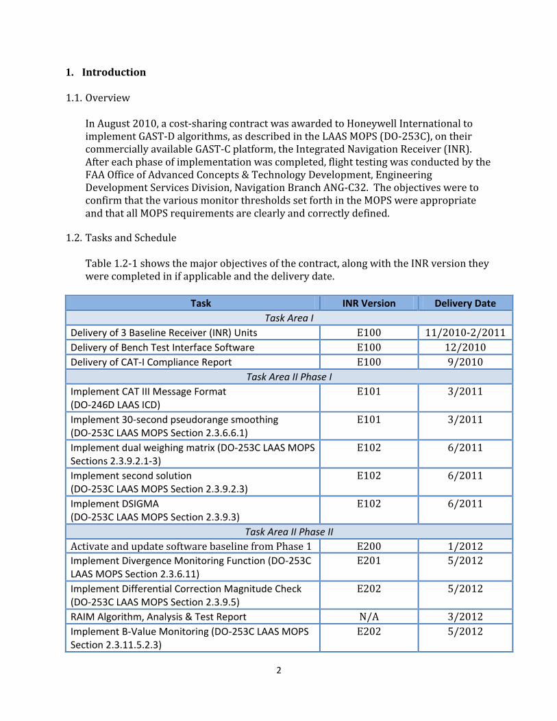
1.2. Tasks and Schedule
Table 1.2-1 shows the major objectives of the contract, along with the INR version they were completed in if applicable and the delivery date.
Task INR Version Delivery Date
Task Area I
Delivery of 3 Baseline Receiver (INR) Units E100 11/2010-2/2011
Delivery of Bench Test Interface Software E100 12/2010
Delivery of CAT-I Compliance Report E100 9/2010
Task Area II Phase I
Implement CAT III Message Format (DO-246D LAAS ICD)
E101 3/2011
Implement 30-second pseudorange smoothing (DO-253C LAAS MOPS Section 2.3.6.6.1)
E101 3/2011
Implement dual weighing matrix (DO-253C LAAS MOPS Sections 2.3.9.2.1-3)
E102 6/2011
Implement second solution (DO-253C LAAS MOPS Section 2.3.9.2.3)
E102 6/2011
Implement DSIGMA (DO-253C LAAS MOPS Section 2.3.9.3)
E102 6/2011
Task Area II Phase II
Activate and update software baseline from Phase 1 E200 1/2012
Implement Divergence Monitoring Function (DO-253C LAAS MOPS Section 2.3.6.11)
E201 5/2012
Implement Differential Correction Magnitude Check (DO-253C LAAS MOPS Section 2.3.9.5)
E202 5/2012
RAIM Algorithm, Analysis & Test Report N/A 3/2012
Implement B-Value Monitoring (DO-253C LAAS MOPS Section 2.3.11.5.2.3)
E202 5/2012

3
Implement Fault Detection and Provide Results Data (DO-253C LAAS MOPS Section 2.3.9.6)
E202 5/2012
Task Area II Phase III
Activate and update software baseline from Phase II E300 8/2012
Implement VDB Message Authentication (DO-253C LAAS MOPS Section 2.3.7.3)
E301/E302 10/2012
Table 1.2-1: Contract Objectives
1.3. Report Coverage
This report details the flight testing equipment and procedures used by ANG-C32. Results from flight testing are shared with the goal of confirming that the MOPS requirements have been correctly implemented and validated.
2. Flight Testing The data presented in this report was collected during flight tests at the Wm. J. Hughes Technical Center by the Office of Advanced Concepts & Technology Development, Engineering Development Services Division, Navigation Branch ANG-C32. A description of general flight test procedures follows.
2.1. Test Equipment and Setup
All flight tests were flown in a Convair 580 (N49) equipped with two INR receivers and flown against the LAAS Test Prototype (LTP) ground station or a modified Honeywell SLS- 4000 GBAS ground station. The LTP is the FAA’s primary LAAS Research and Development (R&D) tool and is used to characterize and test performance of a typical LAAS installation in an operational airport environment. The GAST-D requirements necessary to conduct these flight tests have been implemented in the LTP. The HI SLS-4000 system has also been modified to meet the GAST-D requirements necessary for these tests as part of a separate ground system contract running in parallel to the avionics development contract. The INR received the data broadcast from the LTP or the SLS and used this information to assess the accuracy and integrity of the messages, and then computed position, velocity, and time (PVT) information using the same data. This PVT was utilized for the area navigation (RNAV) guidance and for generating instrument landing system (ILS)-look-alike indications to aid the aircraft on an approach.
Airborne equipment consists of two INR shelves, a Ballard data collection system (DCS) and a Z-Extreme truth system. Each INR shelf contains one Honeywell INR receiver, a control head used to tune the receiver and a Sandel navigation electronic display used to show CDI deviations. The INR receiver requires a 429 input from an Inertial
4
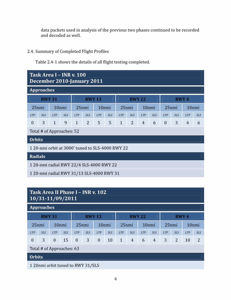
Reference System to provide the PVT output. The Convairs use a custom Honeywell HG-1095 Laser Ref IRS which used two extra bits of data resolution in place if SDI bits. This requires the Ballard DCS to take the output of the IRS, modify the 429 words and retransmit to the INR.
The Ballard DCS consists of a twelve channel 429 receive module, four channel 429 transmit module and a 4 channel rs-232/422 receive module and an ESE-291 GPS based time code generator. All 429 and RS-232 ports transmitted from the INR were collected and time stamped by the DCS and saved on a four gigabyte compact flash card. The DCS has an additional function of modifying some of the INR 429 messages and transmitting them to the Convair’s MLS port to be displayed on the ship’s CDI. This is the only way of displaying CDI information to the pilots.
The Z-Extreme is a dual frequency receiver that provides truth GPS measurements on the test aircraft and ground, independent of the GBAS equipment. A ground-based Z-extreme is used for reference and will be connected to a precision surveyed antenna. Post-processing of the data collected by this system provides accurate aircraft position over the course of a flight.
2.2. Flight Test Objectives/Profiles
The objective of these flight tests was to evaluate the performance of the INR receiver in a fault-free environment. Six sets of flight tests were conducted during evaluation of the INR. One set of flight testing was completed after completion of Task Area I, one after Task Area II Phase 1, two during and after completion of Phase 2, and two during and after completion of Phase 3. Flight tests generally include a 20 mile orbit flown to measure VDB signal strength and verify the availability of FAS data at all four runway ends at ACY. Additionally, 20 mile radials –using runway 13-31 or runway 04-22 will be flown at approximately 3000 feet above ground level (AGL). These radials are flown to establish any VDB nulls. All approaches flown during testing will be straight-in at 3-degrees, and ILS-like. Approaches will start at either 10 or 25nmi from runway threshold. There are always several 25nmi approaches to each runway to confirm Dmax, which is set at 23.7 miles. This requires flying out of coverage and turning in to the runway approach at an altitude of 7000 feet to capture the glideslope within the Dmax range. All approaches were flown in Visual Flight Rules (VFR) and were flown either manually or coupled to the flight director, at the discretion of the pilot. Aircraft speed was approximately 170 knots.
Flight testing phases usually took place over a two week period, consisting of up to ten weekdays of available flight time. This allowed time for missed days due to weather or airplane maintenance issues if necessary. Exact numbers of approaches to each runway and of 10 or 25nmi length vary from flight test to flight test, but the following is a general guideline of the profiles flown:

5
1) Two 20nmi orbits 2) Four 20nmi radials 3) Four 25nmi approaches to RWY 31 4) Four 25nmi approaches to RWY 13 5) Four 25nmi approaches to RWY 04 6) Four 25nmi approaches to RWY 22 7) Twelve 10nmi approaches to RWY 31 8) Twelve 10nmi approaches to RWY 13 9) Twelve 10nmi approaches to RWY 04 10) Twelve 10nmi approaches to RWY 22
2.3. Additional Data Collection and Analysis for Task Area II Flight Testing
During Task Area II flight testing, additional data collection and analysis took place in order to observe data resulting from the new implementation of GAST-D algorithms. This data is made available by the modified INR.
2.3.1. Task Area II Phase I Flight Testing INR data packet 0x5f, “GBASD Position Solutions”, was recorded during this phase of flight testing. This packet includes 30- and 100-second position solutions, as well as DSIGMA values DLAT and DVERT. This data was decoded and plotted. Any DSIGMA values greater than the two meter threshold indicated in the MOPS were further investigated, as were any anomalies in the position solutions.
2.3.2. Task Area II Phase II Flight Testing
In addition to the data collected during Task Area II Phase I flight testing, data packets 0xAC “HPDCM”, 0xB9 “RRFM Parameters”, and 0xBA “FD GBAS SV Addition” were recorded. The HPDCM (Differential Correction Magnitude Check) packet provides 30- and 100-second values for the HPDCM monitor. This data was decoded and compared to the 200 meter threshold indicated in the MOPS. In this phase, values from the RRFM (Reference Receiver Fault Monitoring) and FD GBAS SV Addition (Fault Detection for SV Addition) packet were used to help determine
appropriate values for the σD_VERT and σD_LAT values needed by the RRFM algorithm. 2.3.3. Task Area II Phase III Flight Testing
For Phase III flight tests, INR data packet 0xBB “VDB Message Authentication Parameters” was decoded for analysis. This packet contains information on the slot group definition, SSIDs, and age of the Type 2 message, as well as flags for the various VDB authentication failures that can occur. The RRFM data packet, 0xB9,
was updated for this phase to include computed values for σD_VERT and σD_LAT . The
6
data packets used in analysis of the previous two phases continued to be recorded and decoded as well.
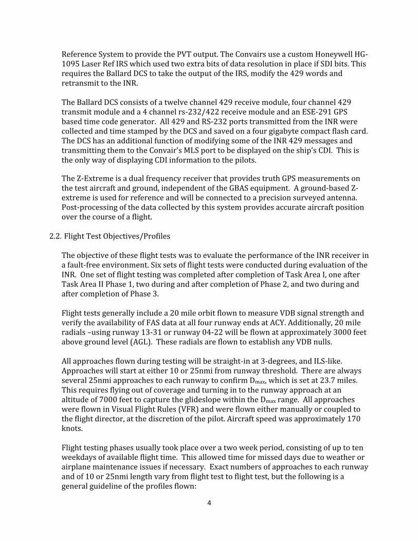
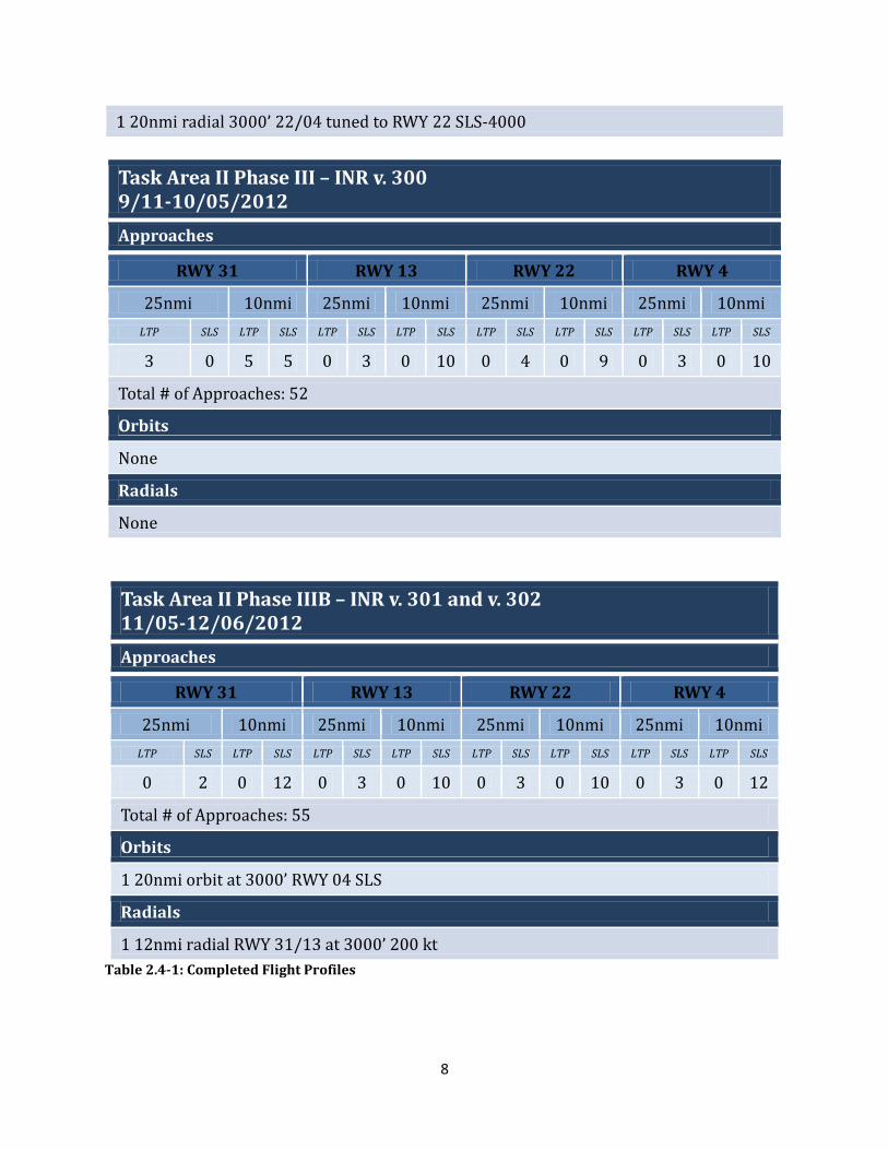
2.4. Summary of Completed Flight Profiles
Table 2.4-1 shows the details of all flight testing completed.
– -
LTP SLS LTP SLS LTP SLS LTP SLS LTP SLS LTP SLS LTP SLS LTP SLS
0 3 1 9 1 2 5 5 1 2 4 6 0 3 4 6
1 20-nmi orbit at 3000’ tuned to SLS-4000 RWY 22
1 20-nmi radial RWY 22/4 SLS-4000 RWY 22
1 20-nmi radial RWY 31/13 SLS-4000 RWY 31
– -
LTP SLS LTP SLS LTP SLS LTP SLS LTP SLS LTP SLS LTP SLS LTP SLS

7
– -
LTP SLS LTP SLS LTP SLS LTP SLS LTP SLS LTP SLS LTP SLS LTP SLS
– -
LTP SLS LTP SLS LTP SLS LTP SLS LTP SLS LTP SLS LTP SLS LTP SLS
2 1 2 6 3 0 5 5 3 0 0 14 3 0 5 5
-
8
-
– -
LTP SLS LTP SLS LTP SLS LTP SLS LTP SLS LTP SLS LTP SLS LTP SLS
3 0 5 5 0 3 0 10 0 4 0 9 0 3 0 10
None
None
– -
LTP SLS LTP SLS LTP SLS LTP SLS LTP SLS LTP SLS LTP SLS LTP SLS
0 2 0 12 0 3 0 10 0 3 0 10 0 3 0 12
1 20nmi orbit at 3000’ RWY 04 SLS
1 12nmi radial RWY 31/13 at 3000’ 200 kt
Table 2.4-1: Completed Flight Profiles

9
3. Task Area I – GAST C Compliance and Performance
Task Area I focused on the delivery and testing of baseline CAT-I INR units, with no
CAT-III implementation completed. Flight testing as described in Section 2.1 on the
CAT-I baseline INR was conducted in December 2010 and January 2011. Only one INR
was tested during this phase, as only one INR had been delivered at the time of the
flights.
The INR behaved as expected, with no indication that it was not in compliance with
GAST-C requirements. The CAT-I compliance report provided by HI was reviewed and
no errors or omissions were noted.
The flight profiles completed during testing of the CAT-I INR (v. E100) are listed in
Table 2.4-1. Plots of system accuracy are typically completed for all ANG-C32 flight
testing and are shown here. The navigation sensor error computed is the difference in
the GLS deviations from the INR and the post-processed TSPI deviations. NSE data is
subject to latency as allowed in MOPS 2.3.11.5.1.3. Figures 3-1 and 3-2 are ensemble
plots of the horizontal and vertical NSE data from all 52 approaches completed during
this phase of testing. As both 10nmi and 25nmi approaches are shown, various start
points can be seen in the data traces. This is also apparent in the Vertical NSE plot
(Figure 3-2), where the start of an approach often correlates with a spike in error as the
pilot turns onto the path. These NSE results are typical of what is seen in previous CAT-
I flight tests using another CAT-I receiver. Figures 3-3 and 3-4 show horizontal and
vertical PVT accuracy from the same set of CAT-I approaches. The data in these plots
has been corrected for latency; they are shown to illustrate the degree of accuracy that
is possible when latency is not a factor.

10
Figure 3-1: Ensemble plot of horizontal NSE data from all approaches flown for INR CAT-I compliance
testing. 52 total runs shown including both LTP and SLS-4000 approaches.
Figure 3-2: Ensemble plot of vertical NSE data from all approaches flown for INR CAT-I compliance
testing. 52 total runs shown including both LTP and SLS-4000 approaches.

11
Figure 3-3: Ensemble plot of horizontal PVT from all approaches flown for INR CAT-I compliance
testing. 52 total runs shown including both LTP and SLS-4000 approaches.
12
Figure 3-4: Ensemble plot of horizontal PVT from all approaches flown for INR CAT-I compliance
testing. 52 total runs shown including both LTP and SLS-4000 approaches.
4. Task Area II: Implementation of GAST-D Protocols for MOPS Validation
The goal of having GAST-D protocols implemented on a commercial receiver such as the
INR was to validate the new requirements from the LAAS MOPS, DO-253C. The work
done in Task Area II focused on ensuring that the language in the MOPS was clear and
correct, that the new monitors were feasible to implement, and that the thresholds
chosen were appropriate and do not cause flagging or loss of service during nominal
conditions. This section details the results of the Task Area II work on a requirement-
by-requirement basis. Navigation Sensor Error results from flights with the modified
INR are also provided.
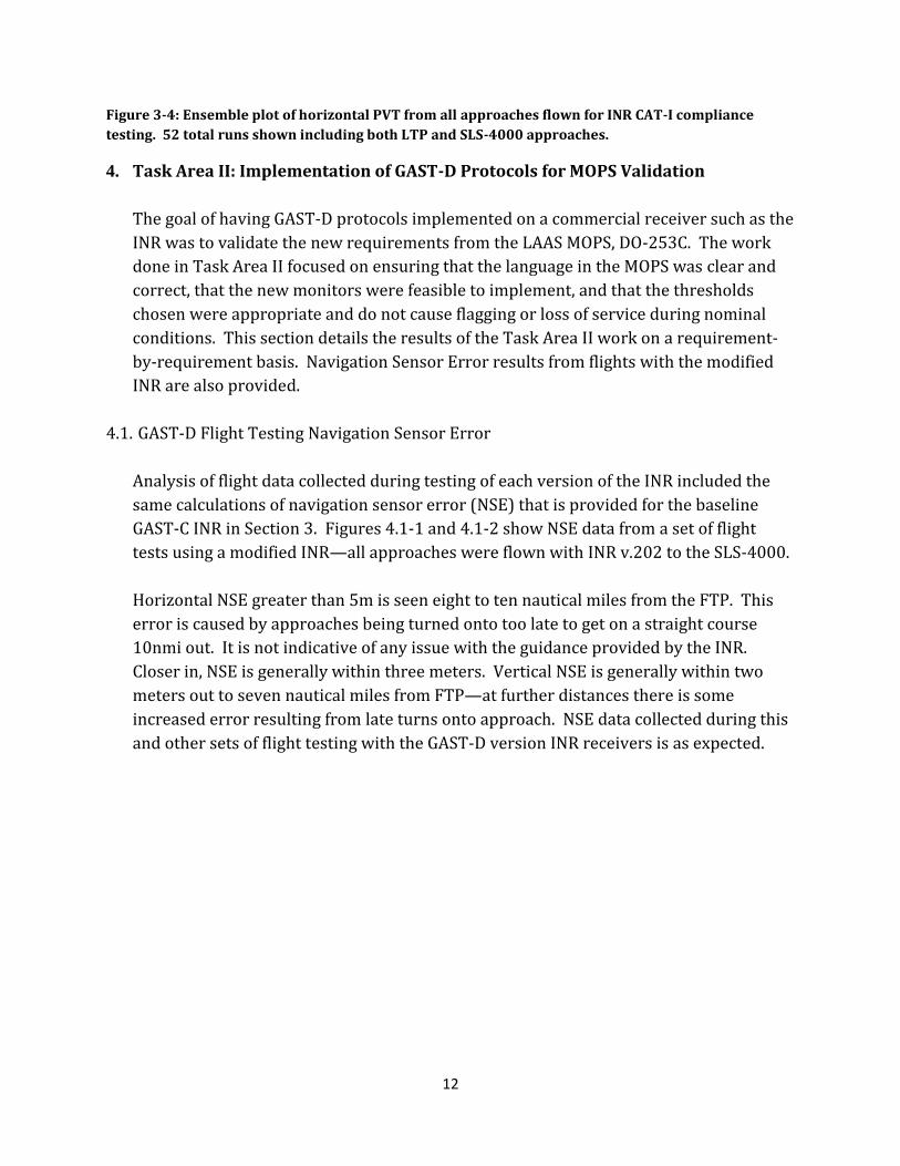
4.1. GAST-D Flight Testing Navigation Sensor Error
Analysis of flight data collected during testing of each version of the INR included the
same calculations of navigation sensor error (NSE) that is provided for the baseline
GAST-C INR in Section 3. Figures 4.1-1 and 4.1-2 show NSE data from a set of flight
tests using a modified INR—all approaches were flown with INR v.202 to the SLS-4000.
Horizontal NSE greater than 5m is seen eight to ten nautical miles from the FTP. This
error is caused by approaches being turned onto too late to get on a straight course
10nmi out. It is not indicative of any issue with the guidance provided by the INR.
Closer in, NSE is generally within three meters. Vertical NSE is generally within two
meters out to seven nautical miles from FTP—at further distances there is some
increased error resulting from late turns onto approach. NSE data collected during this
and other sets of flight testing with the GAST-D version INR receivers is as expected.

13
Figure 4.1-1: Ensemble of Horizontal NSE Data from 31- approaches to the SLS-4000 with INR v.202.
Figure 4.1-2: Ensemble of Vertical NSE Data from 31 approaches to the SLS-4000 with INR v.202.

14
Figure 4.1-3: Ensemble of Vertical NSE Data from 55 approaches to the SLS-400 with INR v.301/302.
4.2. Dual Solution Ionospheric Gradient Monitor (DSIGMA)
DO-253C LAAS MOPS Section 2.3.9.3
The dual solution ionospheric gradient monitor was implemented in INR v. E102 and
activated in v. E200, allowing for the collection of DSIGMA data from 286 approaches
over the course of flight testing.
DSIGMA results during flight testing of INR v. E102 and E200 were impacted by errors
in both the INR and the LTP ground code. The INR was incorrectly using data from
Type 1 messages from one frame and Type 11 messages from another to calculate DLAT
and DVERT in some situations. This caused several sudden jumps in DSIGMA values
during this phase of flight testing, including one instance where DVERT exceeded the 2
meter threshold (Figure 4.1-1). As this error was not discovered until flight testing on
v. E200 had begun, it was corrected in version E201. Post-processing of flight test data
also revealed that the LTP ground station sends erroneous range rate corrections for
satellites when there is a change in the satellites tracked by the LTP references. ANG-
C32 was unable to correct this error during the course of the INR development
contract. For this reason the HI SLS-4000 system was heavily favored during the latter
flight tests. The LTP was only flown when the SLS was not available in GAST-D mode.
Figure 4.1-1 shows an event where DSIGMA exceeded 2m due to errors in the LTP
broadcast and application of corrections by the INR. In addition to the actual break in
threshold, several of the other outliers in the data were traced back to the same errors.

15
Figure 4.1-1: 3 25nmi & 10 10nmi approaches to RWY04 at ACY. Both INRs tuned to the FAA LTP
throughout flight. DSIGMA threshold of 2m is exceeded on both INRs at approximately 228400
seconds.
Figure 4.1-2 shows a composite plot of all DSIGMA values collected during flight testing of
INR versions E300, E301, and E302. Data is included as long as the plane is airborne and
GAST-D is the selected (not necessarily active) service type. The mean lateral DSIGMA
value for the flight tests represented in this figure was 0.0782m (INR #1 0.0782m and INR
#2 0.0803m); mean vertical DSIGMA was 0.1748m (INR #1 0.1789m and INR #2 0.1707m).
This indicates that the two INRs have similar performance with regards to the DSIGMA
algorithm, and that in general the DSIGMA outputs are well below the 2m threshold.

16
Figure 4.1-2: Composite plot of all DSIGMA data points collected during flight testing of INR v. E300,
E301, and E302.
There is one instance where the vertical DSIGMA value exceeds the 2m threshold. This
instance occurred on INR #1 during flight testing of INR v. E301 on 12/03/2012. INR #2
showed similar performance at a slightly lesser magnitude. DSIGMA data from this flight is
shown in Figure 4.1-3. This flight consisted of three 25nmi and eight 10nmi approaches to
ACY RWY 22 with both INRs tuned to the SLS-4000. The active approach service type is
shown in the plot in green. It can be seen going from ‘2’ for GAST-D to ‘1’ for GAST-C when
the vertical DSIGMA value on INR #1 exceeds 2m. The AAST can also be seen dropping to
‘0’ for navigation mode four times when the aircraft is outside of DMAX during 25nmi
approaches. The rise and fall in DSIGMA values around the time of the flag appears to be
gradual in nature, rather than the result of a sudden jump. Further investigation by
Honeywell has revealed that this spike resulted from a period of high VDOP /HDOP. This
was the result of the loss of several tracked satellites during a flight maneuver. Though the
maneuver did not happen coincident with the spike in DSIGMA, the CCD filters took over
eight minutes to settle when these satellites were again tracked, such that they could not be
used for that span of time. This issue is addressed further in Section 4.4.

17
Figure 4.1-3: DSIGMA data for flight in which only observed incident of DSIGMA_vert > 2m occurred.
4.3. Differential Correction Magnitude Check
DO-253C LAAS MOPS Section 2.3.9.5
The differential correction magnitude check was implemented in INR v. E200 and
activated in INR v. E300. This algorithm requires the calculation of a horizontal
position differential correction magnitude (HPDCM). If the HPDCM value exceeds
200m the airborne equipment must remove or flag invalid all deviations and
differential PVT that are determined using the LAAS differential corrections. HI
questioned the wording of this algorithm in the MOPS at RTCA. There was confusion
about which set of smoothed pseudoranges (100- or 30-second) should be used in
computing the HPDCM. A decision was made to use the 100-second smoothed
pseudoranges in calculating the value that could cause a flag on the differential PVT
outputs and the 30-second smoothed pseudoranges in calculating a value that could
flag the deviation outputs. This monitor was activated in v. E300 such that a failure
would cause a demotion to Navigation mode. The receiver returns to the applicable
GBAS mode when the failure condition is no longer present.
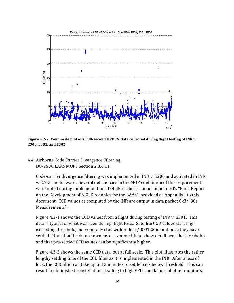
The figures below show, respectively, the 100-second and 30-second derived HPDCM
values during flight testing of INR v. E300, E301, and E302, the versions in which the
differential correction magnitude check was activated. The data shown is a
compilation of all recorded points during flight tests of these versions. The difference
in number of samples is due to the 100-second HPDCM values used for the differential
PVT being output at 1Hz while the 30-second HPDCM values used for the deviations

18
are output at 10Hz. Both sets of data show a maximum HPDCM value of approximately
25m, far beneath the 200m threshold of the monitor. Mean HPDCM for the 100-second
derived values is 2.8335m, mean for the 30-second derived values is 2.4158m.
Figure 4.2-1: Composite plot of all 100-second HPDCM data collected during flight testing of INR v.
E300, E301, and E302.
19
Figure 4.2-2: Composite plot of all 30-second HPDCM data collected during flight testing of INR v.
E300, E301, and E302.
4.4. Airborne Code Carrier Divergence Filtering
DO-253C LAAS MOPS Section 2.3.6.11
Code-carrier divergence filtering was implemented in INR v. E200 and activated in INR
v. E202 and forward. Several deficiencies in the MOPS definition of this requirement
were noted during implementation. Details of these can be found in HI’s “Final Report
on the Development of AEC D Avionics for the LAAS”, provided as Appendix I to this
document. CCD values as computed by the INR are output in data packet 0x3f “30s
Measurements”.
Figure 4.3-1 shows the CCD values from a flight during testing of INR v. E301. This
data is typical of what was seen during flight tests. Satellite CCD values start high,
exceeding threshold, but generally stay within the +/-0.0125m limit once they have
settled. Note that the data shown here is zoomed-in to show detail near the thresholds
and that pre-settled CCD values can be significantly higher.
Figure 4.3-2 shows the same CCD data, but at full scale. This plot illustrates the rather
lengthy settling time of the CCD filter as it is implemented in the INR. After a loss of
lock, the CCD filter can take up to 12 minutes to settle back below threshold. This can
result in diminished constellations leading to high VPLs and failure of other monitors,
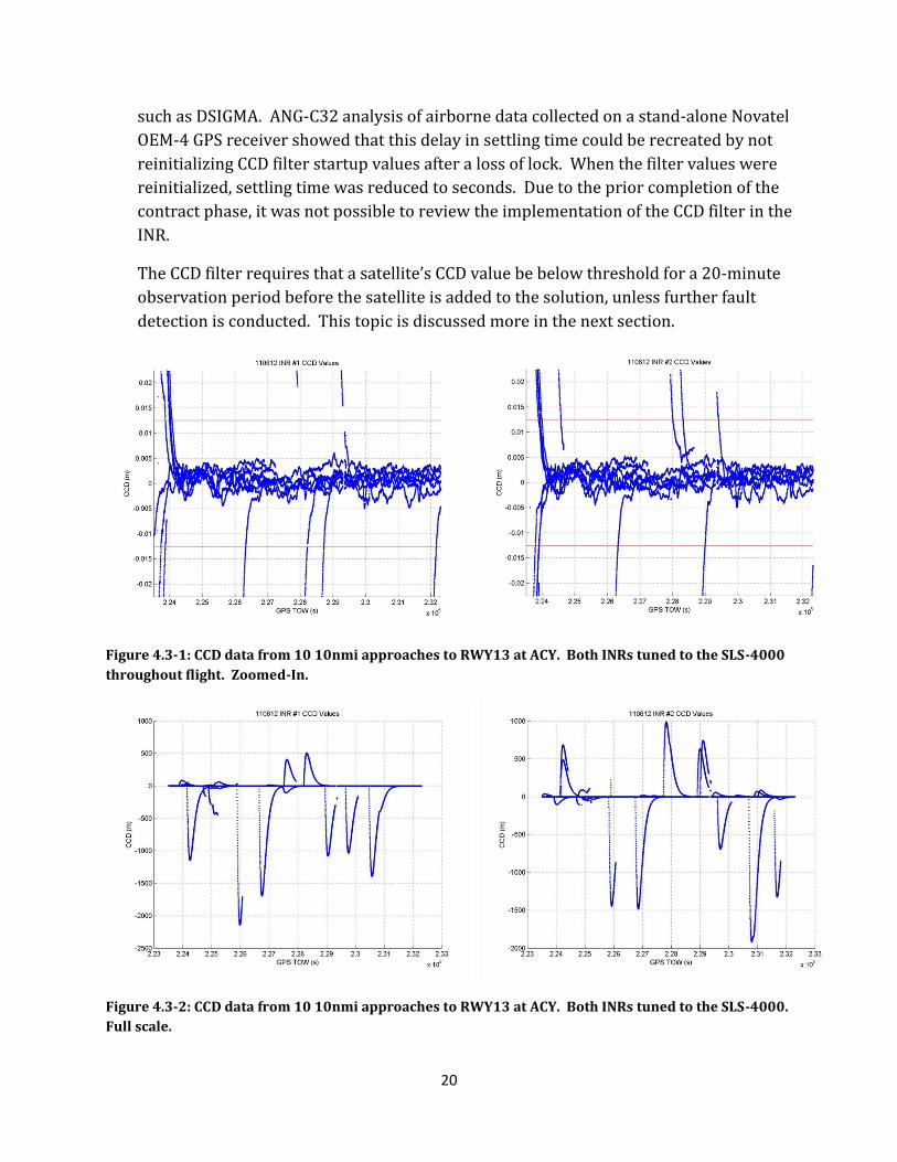
20
such as DSIGMA. ANG-C32 analysis of airborne data collected on a stand-alone Novatel
OEM-4 GPS receiver showed that this delay in settling time could be recreated by not
reinitializing CCD filter startup values after a loss of lock. When the filter values were
reinitialized, settling time was reduced to seconds. Due to the prior completion of the
contract phase, it was not possible to review the implementation of the CCD filter in the
INR.
The CCD filter requires that a satellite’s CCD value be below threshold for a 20-minute
observation period before the satellite is added to the solution, unless further fault
detection is conducted. This topic is discussed more in the next section.
Figure 4.3-1: CCD data from 10 10nmi approaches to RWY13 at ACY. Both INRs tuned to the SLS-4000
throughout flight. Zoomed-In.
Figure 4.3-2: CCD data from 10 10nmi approaches to RWY13 at ACY. Both INRs tuned to the SLS-4000.
Full scale.
21
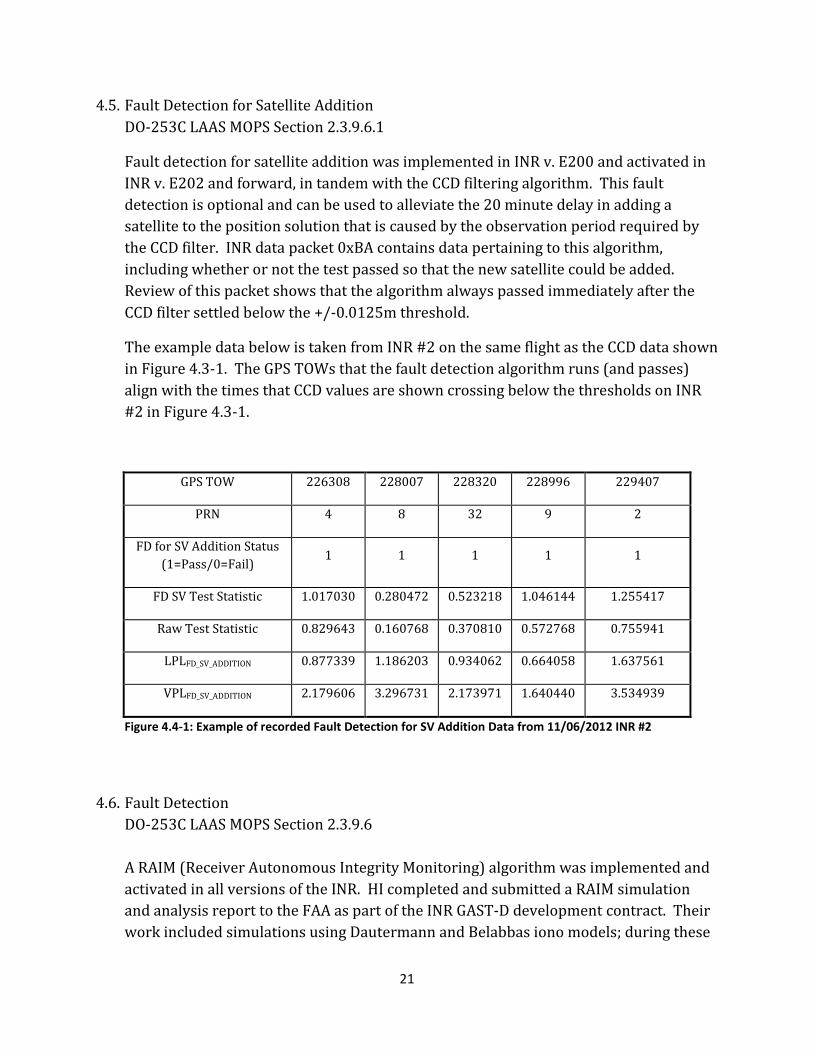
4.5. Fault Detection for Satellite Addition
DO-253C LAAS MOPS Section 2.3.9.6.1
Fault detection for satellite addition was implemented in INR v. E200 and activated in
INR v. E202 and forward, in tandem with the CCD filtering algorithm. This fault
detection is optional and can be used to alleviate the 20 minute delay in adding a
satellite to the position solution that is caused by the observation period required by
the CCD filter. INR data packet 0xBA contains data pertaining to this algorithm,
including whether or not the test passed so that the new satellite could be added.
Review of this packet shows that the algorithm always passed immediately after the
CCD filter settled below the +/-0.0125m threshold.
The example data below is taken from INR #2 on the same flight as the CCD data shown
in Figure 4.3-1. The GPS TOWs that the fault detection algorithm runs (and passes)
align with the times that CCD values are shown crossing below the thresholds on INR
#2 in Figure 4.3-1.
GPS TOW 226308 228007 228320 228996 229407
PRN 4 8 32 9 2
FD for SV Addition Status
(1=Pass/0=Fail) 1 1 1 1 1
FD SV Test Statistic 1.017030 0.280472 0.523218 1.046144 1.255417
Raw Test Statistic 0.829643 0.160768 0.370810 0.572768 0.755941
LPLFD_SV_ADDITION 0.877339 1.186203 0.934062 0.664058 1.637561
VPLFD_SV_ADDITION 2.179606 3.296731 2.173971 1.640440 3.534939
Figure 4.4-1: Example of recorded Fault Detection for SV Addition Data from 11/06/2012 INR #2
4.6. Fault Detection
DO-253C LAAS MOPS Section 2.3.9.6
A RAIM (Receiver Autonomous Integrity Monitoring) algorithm was implemented and
activated in all versions of the INR. HI completed and submitted a RAIM simulation
and analysis report to the FAA as part of the INR GAST-D development contract. Their
work included simulations using Dautermann and Belabbas iono models; during these

22
simulations no false alerts were observed. Missed detection tests were also run and no
missed alerts were observed. The details of these tests and the results can be found in
“Evaluation of GBAS Fault Detection Performance Introduction”, included as an
appendix in the HI “Final Report on the Development of AEC D Avionics for the LAAS”.
Though this fault detection is only required for GAST-D equipment, HI believes that it
would be useful for GAST-C equipment as well in detecting local causes of erroneous
measurements.
RAIM status is available in INR output data packet 0x31 “GNSS Status”. This value was
collected during all flight testing, and no RAIM alerts were observed.
4.7. Reference Receiver Fault Monitoring (RRFM)
DO-253C LAAS MOPS 2.3.11.5.2.3
Work on Reference Receiver Fault Monitoring began in INR v. E200. This version
computed and output all parameters used by the algorithm except for σD_VERT and
σD_LAT, as a decision on how to compute these values had not yet been determined. INR
v. E201 added outputs for three different possible computations of σD_VERT and σD_LAT,
respectively considering ionospheric variance only, ionospheric variance and
multipath, and ionospheric variance, multipath, and receiver noise.
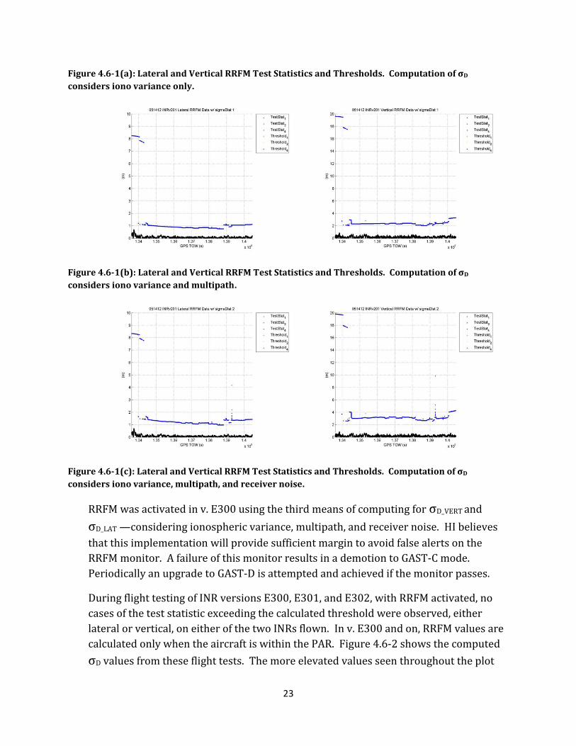
Figure 4.6-1, below, shows examples of RRFM results using each of the three
calculations for σD_VERT and σD_LAT. This data was collected during flight testing of INR v.
E201 on 5/14/2012. During this flight the INRs were tuned to the SLS-4000—data is
from five 10nmi approaches to RWY 13 followed by two 10nmi approaches to RWY 22.
RRFM values are computed regardless of aircraft position in this version. Data at the
start of each plot was recorded while the airplane was on the ground. Accounting for
multipath allows the thresholds to be inflated during this time.
23
Figure 4.6-1(a): Lateral and Vertical RRFM Test Statistics and Thresholds. Computation of σD
considers iono variance only.
Figure 4.6-1(b): Lateral and Vertical RRFM Test Statistics and Thresholds. Computation of σD
considers iono variance and multipath.
Figure 4.6-1(c): Lateral and Vertical RRFM Test Statistics and Thresholds. Computation of σD
considers iono variance, multipath, and receiver noise.
RRFM was activated in v. E300 using the third means of computing for σD_VERT and
σD_LAT —considering ionospheric variance, multipath, and receiver noise. HI believes
that this implementation will provide sufficient margin to avoid false alerts on the
RRFM monitor. A failure of this monitor results in a demotion to GAST-C mode.
Periodically an upgrade to GAST-D is attempted and achieved if the monitor passes.
During flight testing of INR versions E300, E301, and E302, with RRFM activated, no
cases of the test statistic exceeding the calculated threshold were observed, either
lateral or vertical, on either of the two INRs flown. In v. E300 and on, RRFM values are
calculated only when the aircraft is within the PAR. Figure 4.6-2 shows the computed
σD values from these flight tests. The more elevated values seen throughout the plot

24
are due to the inflation of the σs for multipath when the aircraft is on the ground; each
spike correlates to the data collection at the start of a flight test. Figures 4.6-3 and 4.6-
4 show composites of calculated test statistics and thresholds for lateral and vertical
RRFM tests. The data shown includes all that was collected on both INRs during flight
testing of these versions. Note that SLS RSMU #4 was unavailable. Though data for all
available references is plotted, only data for RSMU #3 is clearly seen due to the
similarity of the values for the three references. The larger magnitude data points line
up with the inflated σD values in Figure 4.6-2.
Figure 4.6-2: Composite plot of all recorded σD values from flight testing of INR v. E300, E301, and
E302.

25
Figure 4.6-3: Composite plot of all Lateral RRFM test statistics and thresholds recorded during flight
testing of INR v. E300, E301, and E302.
Figure 4.6-4: Composite plot of all Vertical RRFM test statistics and thresholds recorded during flight
testing of INR v. E300, E301, and E302.
4.8. VDB Message Authentication Protocols
DO-253C LAAS MOPS Section 2.3.7.3
A set of six VDB Message Authentication Protocols are required for AEC-D equipment.
VDB message authentication protocols (a), (c), (e), & (f) were implemented and
activated in INR v. E301. These require confirming that the SSID matches the slot
indicated by the first character of the RPI in the Type 4 message, that the Type 2
message being used is less than one minute old, and that the FAS data block and the
slot group definition (SGD) do not change at any time after approach selection.
Protocols (b) and (d) require the airborne system to determine which slot a message
was received in, to confirm that the Type 2 message is received in the slot indicated by
the SSID and that all messages are received in slots included in the SGD. HI was unable
to accomplish this reliably using the planned software-based approach. The hardware
changes to the INR that would have been required were outside the scope of this
contract. For this reason, these two protocols were implemented but not activated.
Execution of protocols (a), (c), (e), & (f) was activated in this build such that failure
would result in invalidation of the deviations and differential PVT within two seconds.

26
In v. E301, these become valid again as soon as the failure condition is cleared. The
matter of when these faults should be cleared is not currently covered by DO-253C.
Discussion at RTCA concluded that VDB failure conditions should only be cleared upon
retune.
VDB authentication data was output in INR data packet 0xBB for analysis. Type 2 data
age rarely exceeded two seconds (Type 2 data is sent every two seconds from the SLS-
4000) and RPIs were as expected. No attempt to cause these protocols to fail was
made. Further validation of protocols (b) and (d) may be necessary in the future since
their reliable implementation and activation was not possible within the confines of
this contract.
5. Summary & Future Work
The INR GAST-D development contract sought to implement GAST-D algorithms on the
HI INR. With the exception of two of the six new VDB authentication protocols, these
implementations were successfully completed. HI believes that these two protocols
would be feasible with hardware changes to the INR. The data collected during flight
testing indicates that the monitor thresholds currently specified in the LAAS MOPS DO-
253C do not cause excessive false alerts leading to loss of service during nominal
conditions. Several concerns about the clarity of some MOPS requirements were raised
during implementation and were brought to RTCA for discussion and resolution.
Details of these issues are available in HI’s “Final Report on the Development of AEC D
Avionics for the LAAS”.
There is a possibility for future work to be conducted with the INR if funding becomes
available. This work would focus on improving the airborne receiver’s robustness to
RFI. In addition, tasks such as attempting to induce failures on the new monitors,
reviewing the INR implementation of the CCD filter, implementation of the satellite
geometry screening described in DO-253C section 2.3.94, and completion of VDB
authentication protocol implementation may be considered.

FINAL REPORT
ON
THE DEVELOPMENT OF AIRBORNE EQUIPMENT CLASS (AEC) D AVIONICS FOR
THE LOCAL AREA AUGMENTATION SYSTEM (LAAS)
(Contract # DTFACT-10-D-00016)
SUBMITTED TO
FAA WILLIAM J. HUGHES TECHNICAL CENTER
Service ACQUISITION Group, AJA-47A
ATLANTIC CITY INTERNATIONAL AIRPORT, NJ 08405
January 2013
Honeywell Aerospace
One Technology Center
23500 West 105th
Street
Olathe, KS 66061

Appendix I Page 1
Contents 1. Introduction and Executive Summary 2
2. Updates to the previously certified INR 5
3. Deficiencies in the RTCA/DO-253C 15
4. Lab Tests 17
5. Flight Tests 19
Appendix A: Evaluation of GBAS fault detection performance 37
Appendix B: Ionospheric Model for GBAS Test Data Generation 53
Appendix C: Creating exponentially distributed samples from random numbers that are uniformly
distributed 56
List of Acronyms 58
1. Introduction and Executive Summary 3
2. Updates to INR 6
3. Deficiencies in the DO-253C 16
4. Lab Tests 18
5. Flight Tests 21
Plots from Final Build Delivered (E302): 22
Appendix A: Evaluation of GBAS fault detection performance 29
Appendix B: Ionospheric Model for GBAS Test Data Generation 56
Appendix C – Creating exponentially distributed samples from random numbers that are uniformly
distributed 59
List of Acronyms 61
Appendix I Page 2
1. Introduction and Executive Summary
This report summarizes the work performed under FAA contract (DTFACT-10-D-00016), dated August
18, 2010, to Honeywell Aerospace. Under the auspices of the contract, Honeywell collaborated with
the FAA towards the development of an Airborne Equipment Class (AEC) D avionics prototype. The
objectives of this program were (1) to provide the FAA Engineering Development Services Navigation
Team (ANG-C32) and the SATNAV program office with red label (non-certified) equipment, (2) to
implement and test specified messages and algorithms as described in RTCA DO-246D and DO-253C
documents and finally (3) to provide support to the Navigation Team during flight test, TERPS testing,
procedure development, LAAS Ground Facility testing, flight inspection requirements, and to validate
GBAS Approach Service Type (GAST) D requirements.
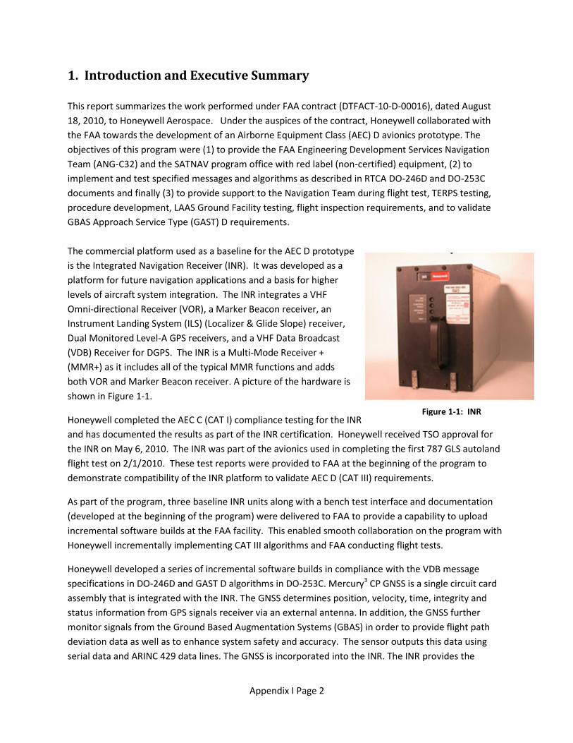
The commercial platform used as a baseline for the AEC D prototype
is the Integrated Navigation Receiver (INR). It was developed as a
platform for future navigation applications and a basis for higher
levels of aircraft system integration. The INR integrates a VHF
Omni-directional Receiver (VOR), a Marker Beacon receiver, an
Instrument Landing System (ILS) (Localizer & Glide Slope) receiver,
Dual Monitored Level-A GPS receivers, and a VHF Data Broadcast
(VDB) Receiver for DGPS. The INR is a Multi-Mode Receiver +
(MMR+) as it includes all of the typical MMR functions and adds
both VOR and Marker Beacon receiver. A picture of the hardware is
shown in Figure 1-1.
Honeywell completed the AEC C (CAT I) compliance testing for the INR
and has documented the results as part of the INR certification. Honeywell received TSO approval for
the INR on May 6, 2010. The INR was part of the avionics used in completing the first 787 GLS autoland
flight test on 2/1/2010. These test reports were provided to FAA at the beginning of the program to
demonstrate compatibility of the INR platform to validate AEC D (CAT III) requirements.
As part of the program, three baseline INR units along with a bench test interface and documentation
(developed at the beginning of the program) were delivered to FAA to provide a capability to upload
incremental software builds at the FAA facility. This enabled smooth collaboration on the program with
Honeywell incrementally implementing CAT III algorithms and FAA conducting flight tests.
Honeywell developed a series of incremental software builds in compliance with the VDB message
specifications in DO-246D and GAST D algorithms in DO-253C. Mercury3 CP GNSS is a single circuit card
assembly that is integrated with the INR. The GNSS determines position, velocity, time, integrity and
status information from GPS signals receiver via an external antenna. In addition, the GNSS further
monitor signals from the Ground Based Augmentation Systems (GBAS) in order to provide flight path
deviation data as well as to enhance system safety and accuracy. The sensor outputs this data using
serial data and ARINC 429 data lines. The GNSS is incorporated into the INR. The INR provides the
Figure 1-1: INR
Appendix I Page 3
required power to the GNSS and uses the GNSS outputs for positioning. The GNSS also uses serial or
ARINC 429 inputs to acquire initial position estimates or optional altitude aiding information. The GNSS
also supports the INR’s predictive RAIM requirements. Only the AEC C baseline software that executes in
the Mercury3 CP GNSS module, a part of the MMR (INR) hardware unit, was modified. Honeywell
verified that various monitor thresholds set forth in DO-253C were appropriate and that most
requirements were clearly defined and were correct. Some additional guidance was needed in the
document for some of the monitors and some requirements were not completely correct. Due to these
deficiencies, Honeywell had to deviate from the MOPS on some requirements. Each deviation was
discussed with the FAA before implementation and details are provided in this report. These short
comings have been presented to RTCA’s SC-159 for further evaluation.
Each software build, including both new and modified AEC C software, was tested in Honeywell’s labs
using developmental hardware. The tested software code was delivered in an object form suitable for
loading into the INR using the bench test interface. Along with each build, an updated Interface Control
Document, describing the output message formats, and MercHost Tool to record the RS-232 data output
by the INR was delivered.
Flight tests were performed by the FAA with each software update. Data from each flight test was
analyzed to observe GAST D performance.
In the following sections, this report summarizes the tasks performed to create AEC D prototype
software, deviations taken from DO-253C while implementing the algorithms for GAST D monitors,
deficiencies found in DO-253C, lab testing performed by Honeywell and flight tests performed by the
FAA.
1.1 Recommendations for Future Activities A few tasks were identified during this program but could not be completed due to timing and funding
constraints. These tasks have been listed below as recommendations for future activities.
a. The flight tests covered ideal case conditions. Trigger Conditions to induce failures of monitors like
RRFM, VDB authentication protocols, etc. that apply to GAST D, need to be created during flight tests.
b. DO-253C requires implementation of airborne CCD filter that needs to settle before measurements
can be included in GBAS mode. CCD filter output takes several minutes to settle. This prevents use of
satellites in GAST D mode and contributed to a DSIGMA failure on a flight test on December 03, 2012.
Details on this failure are provided in section 5 of this report. A study can needs to be performed to
observe the impact of initialization values on the CCD filter or enhancing the filter to accelerate shorten
the settling period.
c. VDB Authentication Protocols ‘b’ and ‘d’ were not completely implemented in this program as they
required a hardware modification to the INR which was not performed. They will need to be
implemented in the production unit and further testing of these protocols needs to be performed then.
Appendix I Page 4
d. The addition of a GBAS Fault Detection test section to RTCA/DO-253C needs to be discussed with
RTCA. See Appendix A of this report for details.
e. As a part of this program, Honeywell has not implemented the geometry screening requirements
related to the GASTD monitors. This can be implemented and their effects on GASTD availability can be
evaluated.
Appendix I Page 5
2. Updates to the previously certified INR During this project the baseline AEC C INR, previously certified to comply with TSO-C161 and DO-253A
for GAST C operation, was modified to support GAST D operations. In addition, a laboratory test
environment (a “Bench Test Interface”) was created to support the evaluation of the new and modified
functionality.
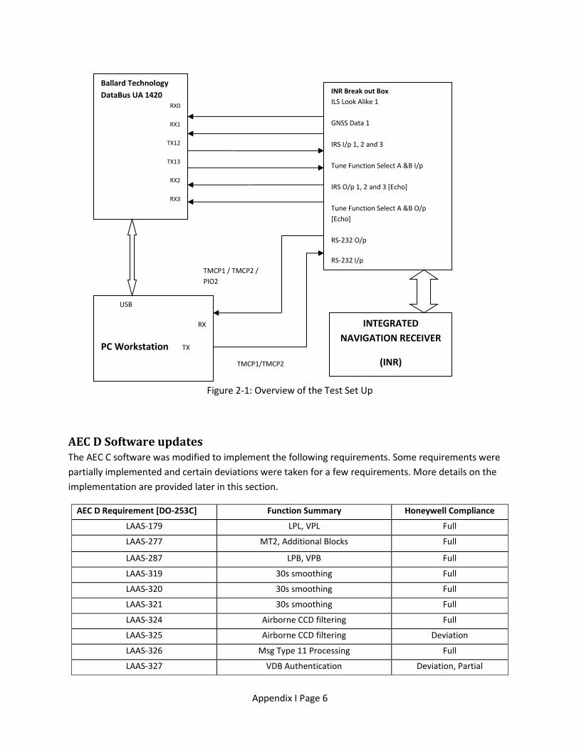
Bench Test Interface The bench test interface was developed and tested to support software loading of the GNSS
module without removing the module from the LRU at the FAA laboratory facilities. This test
set-up involved the use of the INR break-out box (p/n: 071-00265-0000) in conjunction with the
Ballard Technology’s Avionics Data Bus Model UA 1420. The INR’s break-out box provides
interfaces to all data from the INR. It is connected to the INR by a cable harness. There are
several pins provided on the break-out box that are intended to control the INR’s discrete inputs,
allow access to fault logs and to be used in loading software in the GNSS module.
The PC tool, ‘MercHost’, is used to view data from the INR RS-232 ports and to record and
examine in real-time various GPS parameters that can facilitate testing and debugging the
functions of the GNSS. MercHost was updated to support new AEC D/GAST D messages
transmitted by the INR. Ballard Technology’s Co-Pilot 5.20 was used for viewing/changing
ARINC 429 data transmitted and received via the UA 1420.
The MercHost and Co-Pilot software, the assembled and tested bench test interface along with an
INR containing the AEC C baseline software were delivered early in the project. Supporting
documentation such as the interface control document, the INR installation manual, and a
description of AEC C/GACT C compliance testing were also delivered. Figure 2-1 below gives
an overview of the test set-up.
Appendix I Page 6
Figure 2-1: Overview of the Test Set Up
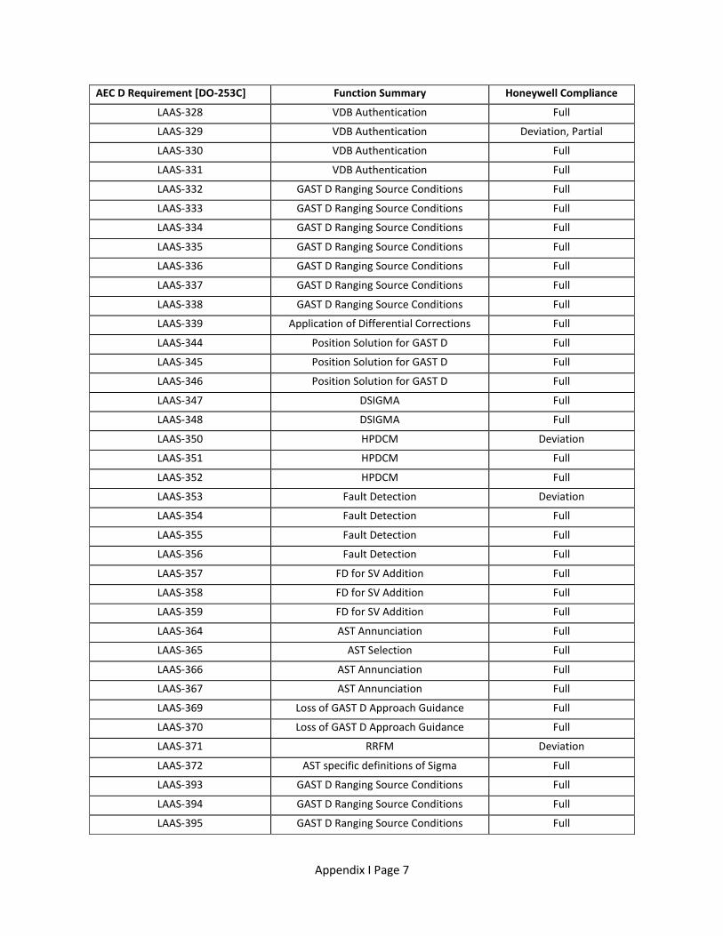
AEC D Software updates The AEC C software was modified to implement the following requirements. Some requirements were
partially implemented and certain deviations were taken for a few requirements. More details on the
implementation are provided later in this section.
AEC D Requirement [DO-253C] Function Summary Honeywell Compliance
LAAS-179 LPL, VPL Full
LAAS-277 MT2, Additional Blocks Full
LAAS-287 LPB, VPB Full
LAAS-319 30s smoothing Full
LAAS-320 30s smoothing Full
LAAS-321 30s smoothing Full
LAAS-324 Airborne CCD filtering Full
LAAS-325 Airborne CCD filtering Deviation
LAAS-326 Msg Type 11 Processing Full
LAAS-327 VDB Authentication Deviation, Partial
Ballard Technology
DataBus UA 1420 RX0
RX1
TX12
TX13
RX2
RX3
INR Break out Box
ILS Look Alike 1
GNSS Data 1
IRS I/p 1, 2 and 3
Tune Function Select A &B I/p
IRS O/p 1, 2 and 3 [Echo]
Tune Function Select A &B O/p
[Echo]
RS-232 O/p
RS-232 I/p
USB
RX
PC Workstation TX
TMCP1/TMCP2
TMCP1 / TMCP2 /
PIO2
INTEGRATED
NAVIGATION RECEIVER
(INR)
Appendix I Page 7
AEC D Requirement [DO-253C] Function Summary Honeywell Compliance
LAAS-328 VDB Authentication Full
LAAS-329 VDB Authentication Deviation, Partial
LAAS-330 VDB Authentication Full
LAAS-331 VDB Authentication Full
LAAS-332 GAST D Ranging Source Conditions Full
LAAS-333 GAST D Ranging Source Conditions Full
LAAS-334 GAST D Ranging Source Conditions Full
LAAS-335 GAST D Ranging Source Conditions Full
LAAS-336 GAST D Ranging Source Conditions Full
LAAS-337 GAST D Ranging Source Conditions Full
LAAS-338 GAST D Ranging Source Conditions Full
LAAS-339 Application of Differential Corrections Full
LAAS-344 Position Solution for GAST D Full
LAAS-345 Position Solution for GAST D Full
LAAS-346 Position Solution for GAST D Full
LAAS-347 DSIGMA Full
LAAS-348 DSIGMA Full
LAAS-350 HPDCM Deviation
LAAS-351 HPDCM Full
LAAS-352 HPDCM Full
LAAS-353 Fault Detection Deviation
LAAS-354 Fault Detection Full
LAAS-355 Fault Detection Full
LAAS-356 Fault Detection Full
LAAS-357 FD for SV Addition Full
LAAS-358 FD for SV Addition Full
LAAS-359 FD for SV Addition Full
LAAS-364 AST Annunciation Full
LAAS-365 AST Selection Full
LAAS-366 AST Annunciation Full
LAAS-367 AST Annunciation Full
LAAS-369 Loss of GAST D Approach Guidance Full
LAAS-370 Loss of GAST D Approach Guidance Full
LAAS-371 RRFM Deviation
LAAS-372 AST specific definitions of Sigma Full
LAAS-393 GAST D Ranging Source Conditions Full
LAAS-394 GAST D Ranging Source Conditions Full
LAAS-395 GAST D Ranging Source Conditions Full
Appendix I Page 8
AEC D Requirement [DO-253C] Function Summary Honeywell Compliance
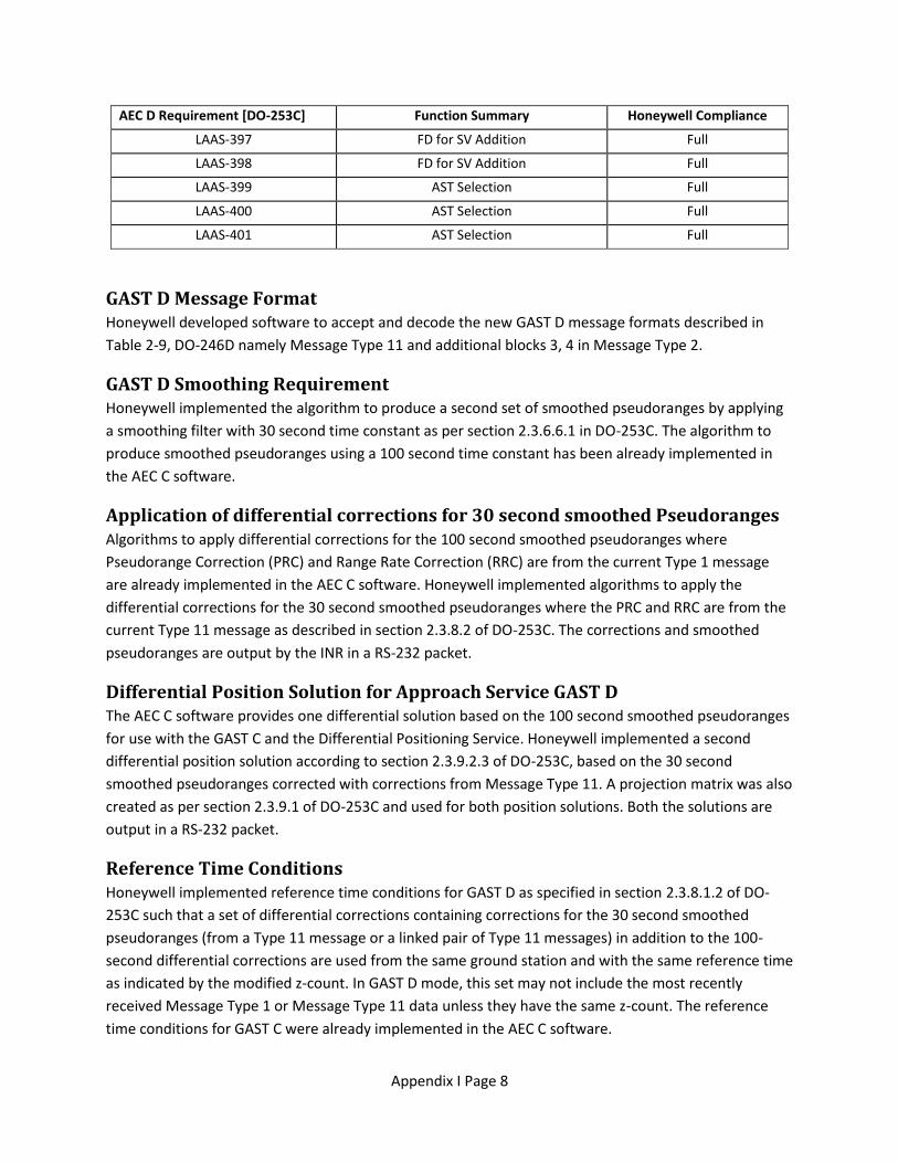
LAAS-397 FD for SV Addition Full
LAAS-398 FD for SV Addition Full
LAAS-399 AST Selection Full
LAAS-400 AST Selection Full
LAAS-401 AST Selection Full
GAST D Message Format Honeywell developed software to accept and decode the new GAST D message formats described in
Table 2-9, DO-246D namely Message Type 11 and additional blocks 3, 4 in Message Type 2.
GAST D Smoothing Requirement Honeywell implemented the algorithm to produce a second set of smoothed pseudoranges by applying
a smoothing filter with 30 second time constant as per section 2.3.6.6.1 in DO-253C. The algorithm to
produce smoothed pseudoranges using a 100 second time constant has been already implemented in
the AEC C software.
Application of differential corrections for 30 second smoothed Pseudoranges Algorithms to apply differential corrections for the 100 second smoothed pseudoranges where
Pseudorange Correction (PRC) and Range Rate Correction (RRC) are from the current Type 1 message
are already implemented in the AEC C software. Honeywell implemented algorithms to apply the
differential corrections for the 30 second smoothed pseudoranges where the PRC and RRC are from the
current Type 11 message as described in section 2.3.8.2 of DO-253C. The corrections and smoothed
pseudoranges are output by the INR in a RS-232 packet.
Differential Position Solution for Approach Service GAST D The AEC C software provides one differential solution based on the 100 second smoothed pseudoranges
for use with the GAST C and the Differential Positioning Service. Honeywell implemented a second
differential position solution according to section 2.3.9.2.3 of DO-253C, based on the 30 second
smoothed pseudoranges corrected with corrections from Message Type 11. A projection matrix was also
created as per section 2.3.9.1 of DO-253C and used for both position solutions. Both the solutions are
output in a RS-232 packet.
Reference Time Conditions Honeywell implemented reference time conditions for GAST D as specified in section 2.3.8.1.2 of DO-
253C such that a set of differential corrections containing corrections for the 30 second smoothed
pseudoranges (from a Type 11 message or a linked pair of Type 11 messages) in addition to the 100-
second differential corrections are used from the same ground station and with the same reference time
as indicated by the modified z-count. In GAST D mode, this set may not include the most recently
received Message Type 1 or Message Type 11 data unless they have the same z-count. The reference
time conditions for GAST C were already implemented in the AEC C software.
Appendix I Page 9
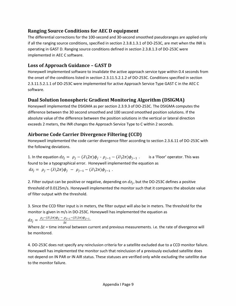
Ranging Source Conditions for AEC D equipment The differential corrections for the 100-second and 30-second smoothed pseudoranges are applied only
if all the ranging source conditions, specified in section 2.3.8.1.3.1 of DO-253C, are met when the INR is
operating in GAST D. Ranging source conditions defined in section 2.3.8.1.3 of DO-253C were
implemented in AEC C software.
Loss of Approach Guidance – GAST D Honeywell implemented software to invalidate the active approach service type within 0.4 seconds from
the onset of the conditions listed in section 2.3.11.5.2.1.2 of DO-253C. Conditions specified in section
2.3.11.5.2.1.1 of DO-253C were implemented for active Approach Service Type GAST C in the AEC C
software.
Dual Solution Ionospheric Gradient Monitoring Algorithm (DSIGMA) Honeywell implemented the DSIGMA as per section 2.3.9.3 of DO-253C. The DSIGMA computes the
difference between the 30 second smoothed and 100 second smoothed position solutions. If the
absolute value of the difference between the position solutions in the vertical or lateral direction
exceeds 2 meters, the INR changes the Approach Service Type to C within 2 seconds.
Airborne Code Carrier Divergence Filtering (CCD) Honeywell implemented the code carrier divergence filter according to section 2.3.6.11 of DO-253C with
the following deviations.
1. In the equation - . is a ‘Floor’ operator. This was
found to be a typographical error. Honeywell implemented the equation as
2. Filter output can be positive or negative, depending on , but the DO-253C defines a positive
threshold of 0.0125m/s. Honeywell implemented the monitor such that it compares the absolute value
of filter output with the threshold.
3. Since the CCD filter input is in meters, the filter output will also be in meters. The threshold for the
monitor is given in m/s in DO-253C. Honeywell has implemented the equation as
Where = time interval between current and previous measurements. i.e. the rate of divergence will
be monitored.
4. DO-253C does not specify any reinclusion criteria for a satellite excluded due to a CCD monitor failure.
Honeywell has implemented the monitor such that reinclusion of a previously excluded satellite does
not depend on IN PAR or IN AIR status. These statuses are verified only while excluding the satellite due
to the monitor failure.

Appendix I Page 10
5. The CCD monitor was activated for both GASTC and GAST D modes, i.e. any satellite whose CCD filter output exceeds the threshold is excluded from precision approach position solution. However, the 20 min observation period for satellite inclusion after the CCD monitor settles, is used only for GAST D. For GASTC, the INR uses measurements as soon as the CCD filter output is below threshold. Note that after Honeywell implemented its algorithm, SC-159 WG2 has determined that a slightly different algorithm is more appropriate.
Horizontal Differential Correction Magnitude Check (HPCM) Honeywell implemented the differential correction magnitude check as per section 2.3.9.5 of DO-253C
with the following deviations:
1. The total correction to the measured pseudorange for satellite ‘i’ is given in DO-253C as
Honeywell implemented the equation for as given in TSO-161a:
2. DO-253C requires the HPDCM to be computed from corrections for pseudoranges for the position
solution being used. In case this monitor fails, deviations and differential PVT need to be invalidated.
DO-253C doesn’t specify whether differential corrections for 30 second smoothed pseudoranges or 100
second smoothed pseudoranges should be selected for HPDCM when a PAN equipment is in GAST C or
GAST D mode.
Since in GAST C, deviations and position are computed from 100 second smoothed pseudoranges and in
GAST D, deviations are computed from 30 second smoothed pseudoranges while position is computed
from 100 second pseudoranges, Honeywell has implemented this monitor such that in GAST C, the
HPDCM computed from corrections for 100 second smoothed pseudoranges( ) are
monitored. In GAST D, HPDCM computed from corrections for 30 second ( ) and 100 second
( ) smoothed pseudoranges are monitored.
The following failure conditions are used: a) In GAST C mode, if > 200m, invalidate deviations and discontinue use of data from the
ground station for position computation.
b) In GAST D mode, if > 200m OR/AND > 200m, invalidate deviations and
discontinue use of data from the ground station for position computation.
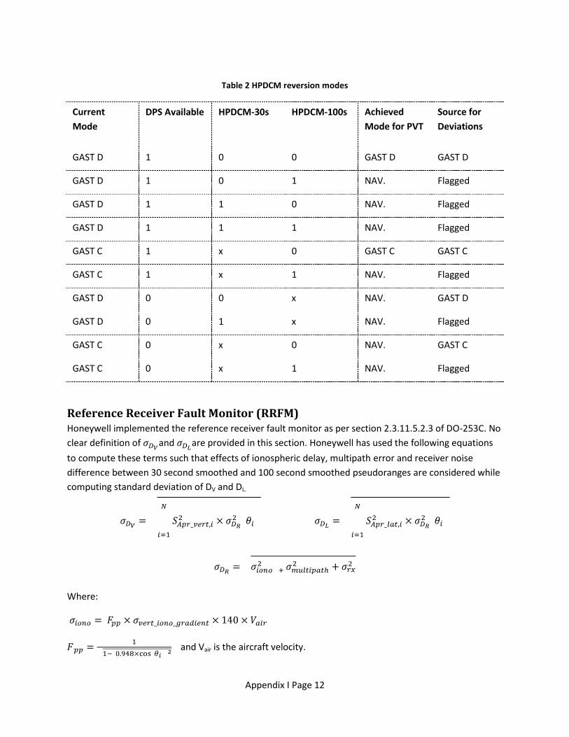
Table 2 below indicates the modes of operation the AEC D software will achieve given various HPDCM
modes. In the table, HPDCM-30s and HPDCM-100s are flags indicating whether HPDCM check failed
when either of the two corrections is used. ‘1’ represents > 200m or ‘True’, ‘0’ indicates that
or ‘False’ and NAV includes both SBAS and Autonomous Navigation modes. ‘x’
indicates that the value in this column can take on any value. DPS Available indicates whether selected
ground station supports differentially corrected positioning service. This field is 0 when RSDS is all 1’s.

Appendix I Page 11
Appendix I Page 12
Table 2 HPDCM reversion modes
Current
Mode
DPS Available HPDCM-30s HPDCM-100s Achieved
Mode for PVT
Source for
Deviations
GAST D 1 0 0 GAST D GAST D
GAST D 1 0 1 NAV. Flagged
GAST D 1 1 0 NAV. Flagged
GAST D 1 1 1 NAV. Flagged
GAST C 1 x 0 GAST C GAST C
GAST C 1 x 1 NAV. Flagged
GAST D 0 0 x NAV. GAST D
GAST D 0 1 x NAV. Flagged
GAST C 0 x 0 NAV. GAST C
GAST C 0 x 1 NAV. Flagged
Reference Receiver Fault Monitor (RRFM) Honeywell implemented the reference receiver fault monitor as per section 2.3.11.5.2.3 of DO-253C. No
clear definition of and are provided in this section. Honeywell has used the following equations
to compute these terms such that effects of ionospheric delay, multipath error and receiver noise
difference between 30 second smoothed and 100 second smoothed pseudoranges are considered while
computing standard deviation of DV and DL.
Where:
and Vair is the aircraft velocity.

Appendix I Page 13
is the airborne receiver’s multipath error when on the ground.
is the airborne receiver’s multipath error in air.
is the elevation angle.
Variance of receiver noise difference between 30 second smoothed and 100 second smoothed
pseudoranges is given as:
is the receiver noise for 30 second smoothed pseudorange.
is the receiver noise for 100 second smoothed pseudorange.
RAIM algorithm, analysis and test report Honeywell determined appropriate Receiver Autonomous Integrity Monitor (RAIM) for differential and
non-differential modes based on the analyzed performance of the Mercury3 CP GNSS receiver hardware
in the INR. A test report containing results of the analysis, describing position and range domain results
is attached in Appendix A.
Fault Detection Honeywell implemented the fault detection (FD) algorithm based in compliance with section 2.3.9.6 of
DO-253C. The FD algorithm is required to have a provide a probability of false alert less than or equal to
per sample but there is no requirement for probability of missed detection.
While DO-253C requires the FD algorithm to be executed only in GAST D mode, Honeywell believes that
the FD algorithm will be useful in detecting local conditions (like multipath) that may lead to faulted
measurements and chose to execute it in GAST C mode as well. In GAST D mode, FD is performed on the
solution that is computed using the 30 second smoothed measurements which have been differentially
corrected using data from Message Type 11. If a fault is detected in GAST D mode, the mode of
operation and thus the Approach Service Type are changed to GAST C. In GAST C mode, FD is performed
on the solution computed using 100 second smoothed measurements that have been differentially
corrected using data from Message Type 1. If a fault is detected in GAST C mode, the INR continues to
operate in GAST C mode but provides the FD annunciation.
Appendix I Page 14
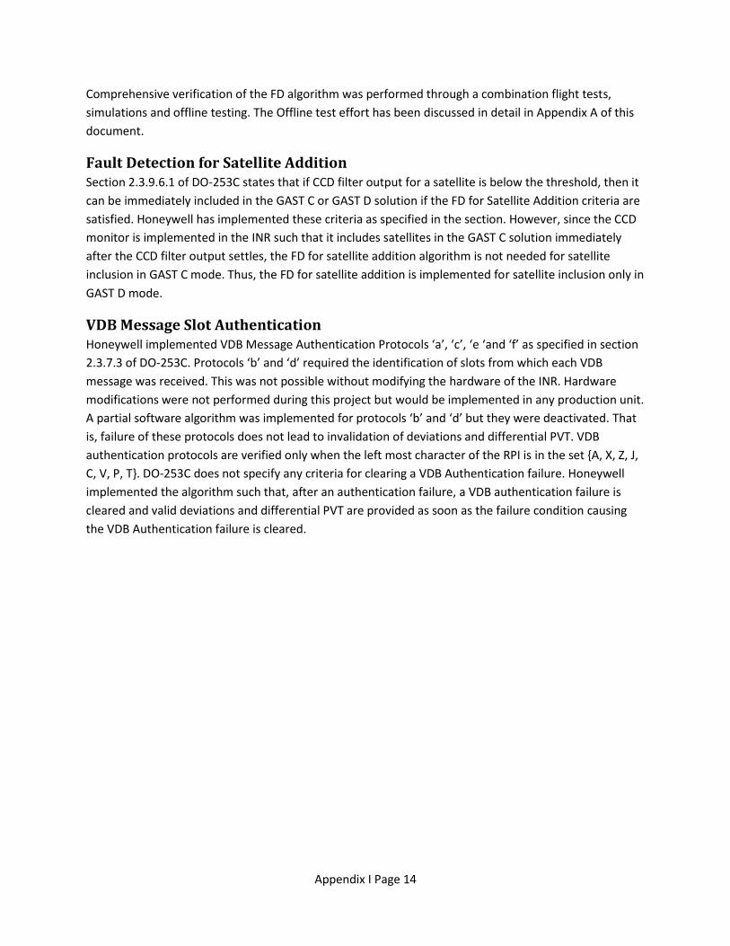
Comprehensive verification of the FD algorithm was performed through a combination flight tests,
simulations and offline testing. The Offline test effort has been discussed in detail in Appendix A of this
document.
Fault Detection for Satellite Addition Section 2.3.9.6.1 of DO-253C states that if CCD filter output for a satellite is below the threshold, then it
can be immediately included in the GAST C or GAST D solution if the FD for Satellite Addition criteria are
satisfied. Honeywell has implemented these criteria as specified in the section. However, since the CCD
monitor is implemented in the INR such that it includes satellites in the GAST C solution immediately
after the CCD filter output settles, the FD for satellite addition algorithm is not needed for satellite
inclusion in GAST C mode. Thus, the FD for satellite addition is implemented for satellite inclusion only in
GAST D mode.
VDB Message Slot Authentication Honeywell implemented VDB Message Authentication Protocols ‘a’, ‘c’, ‘e ‘and ‘f’ as specified in section
2.3.7.3 of DO-253C. Protocols ‘b’ and ‘d’ required the identification of slots from which each VDB
message was received. This was not possible without modifying the hardware of the INR. Hardware
modifications were not performed during this project but would be implemented in any production unit.
A partial software algorithm was implemented for protocols ‘b’ and ‘d’ but they were deactivated. That
is, failure of these protocols does not lead to invalidation of deviations and differential PVT. VDB
authentication protocols are verified only when the left most character of the RPI is in the set {A, X, Z, J,
C, V, P, T}. DO-253C does not specify any criteria for clearing a VDB Authentication failure. Honeywell
implemented the algorithm such that, after an authentication failure, a VDB authentication failure is
cleared and valid deviations and differential PVT are provided as soon as the failure condition causing
the VDB Authentication failure is cleared.

Appendix I Page 15
3. Deficiencies in the RTCA/DO-253C The following describes deficiencies or errors in the MOPS observed during this program.
Airborne Code Carrier Divergence Filtering (CCD) Section 2.3.6.11 in DO-253C describes the Airborne CCD filtering. It has the following deficiencies:
1. In the equation - . is a ‘Floor’ operator. The value of
is usually below 1m. Using a floor operator will make the filter output 0. The floor operation should
be square brackets.
2. Filter output can be positive or negative, depending on , but the DO-253C defines a positive
threshold of 0.0125m/s. A note could be added that the absolute value of the filter output is to be
compared to the threshold.
3. Since the CCD filter input is in meters, the filter output will also be in meters. The threshold for the
monitor is given in m/s in DO-253C. It does not mention that the ‘rate’ of the code carrier divergence is
monitored.
4. DO-253C does not specify any reinclusion criteria for a satellite excluded due to a CCD monitor failure.
It is unclear whether IN PAR and IN AIR states should be monitored for reinclusion of a measurement as
well.
5. DO-253C mentions that a 20 min observation period needs to be applied for satellite inclusion after the CCD monitor settles. This implies that the receiver could stay in Autonomous Nav for several minutes after start-up. This performance is different than that of an AEC C equipment which will immediately enter GAST C mode. So, an AEC D equipment may not provide valid deviations and differential position for 20 minutes at departure while an AEC C equipment will be able to.
Differential Correction Magnitude Check (HPCM) Section 2.3.9.5 in DO-253C lists the requirements for HPDCM. It has the following deficiencies:
1. The total correction to the measured pseudorange for satellite ‘i’ is given in DO-253C as
This doesn’t match the equation in TSO-161a:
2. DO-253C requires the HPDCM to be computed from corrections for pseudoranges for the position
solution being used. It doesn’t require HPDCM to use corrections for 30 second smoothed pseudoranges
in GAST D mode, but requires the deviations to be removed when HPDCM > 200 meters. In GAST C
deviations and position are computed from 100 second smoothed pseudoranges and in GAST D,
deviations are computed from 30 second smoothed pseudoranges while position is computed from 100
second pseudoranges. DO-253C doesn’t specify whether differential corrections for 30 second

Appendix I Page 16
smoothed pseudoranges or 100 second smoothed pseudoranges should be selected for HPDCM when a
PAN equipment is in GAST C or GAST D mode.
Reference Receiver Fault Monitor (RRFM) Section 2.3.11.5.2.3 of DO-253C does not clearly define how the standard deviation of DV and DL should
be computed. No limitations are provided for values of and . DO-253C mentions that the
manufacturer should establish values for and to represent the actual system performance. With
this guidance, each manufacturer can interpret these values differently. One could assume the
maximum value based on highest allowed DV and DL of 2m, or a minimum value of 0m. Computing
standard deviation from observed values can defy the purpose of the monitor as the threshold would be
raised when deviation occurs leading to missed detection. Acceptable assumptions need to be listed in
the document.
Fault Detection Section 2.3.9.6 in DO-253C doesn’t require the FD algorithm to be implemented in GAST C mode.
Honeywell however believes that the FD algorithm will be useful in detecting local conditions (like
multipath) that may lead to faulted measurements. Appendix A also recommends the addition of a test
section for FD in DO-253C.
Fault Detection for Satellite Addition 1. Section 2.3.9.6.1 in DO-253C needs more clarity on when exactly the FD for SV addition needs to be
performed (include start-up time, when receiver is not yet in GBAS mode).
2. Course of action when multiple satellites (that have failed the CCD test in the previous 20 minutes)
become available at the same time needs to be defined.
VDB Message Slot Authentication No guidance is provided in Section 2.3.7.3 in DO-253C for clearing a VDB Authentication failure and
reinstating GAST D mode. It is unclear whether it is okay to use corrections from a GBAS station after a
VDB authentication protocol has failed in the past or re-tuning is required for this.

Appendix I Page 17
4. Lab Tests The software builds delivered during each phase of the project were tested at Honeywell, Olathe. A SLS-
4000 was used to provide VDB messages to the INR. For some tests simulations were used to create
failure conditions which could not be generated with live data. Data from RS-232 packets added to the
software were used for testing. Some of these packets are present in the final build delivered. Long
term testing was performed prior to delivery of the build. A brief description of the testing for each
update is provided below.
Deviation Latency: During the first flight test with the baseline AEC C software, the FAA observed some latency in the
deviations output by the INR. This was analyzed by Honeywell and it was found that the deviation
latency observed in the GAST C flight test was due to the 787 lever arm corrections applied by the AEC C
INR. It was verified that deviation latency complied with requirements specified in section 2.3.11.5.1 in
DO-253C. This was done during the AEC C (CAT I) compliance testing for the INR and the results have
been documented as part of the INR certification.
GAST D Message Format: The following was verified:
1. INR receives and decodes parameters in GBAS Message Type 11 and Message Type 2, Additional Block
3 and additional block 4 correctly as per DO-246D and DO-253C.
2. Maximum and minimum allowed values for each parameter in these messages are received and
parsed correctly.
3. VDB messages are rejected if value of any field is out of range as defined in DO-246D.
4. Message Type 11 is rejected if number of measurements is set to 0 or measurement type is other
than 0.
5. Linked pair message Type 11 is accepted and parsed correctly.
GAST D Smoothing Requirement, Application of differential corrections for 30
second smoothed Pseudoranges, Differential Position Solution for Approach
Service GAST D: Testing was done to ensure that corrections from Message Type 11 were applied to the 30 second
smoothed pseudoranges, a 30 second position solution was computed correctly and receiver achieved
GAST D.
Reference Time Conditions, Ranging Source Conditions for AEC D equipment,
Loss of Approach Guidance – GAST D: Each ranging source condition and loss of Approach guidance condition for GAST D was tested. It was
also verified that in GAST D, the INR uses a set of corrections from Message Type 1 and Message Type 11
with the same z-count.
Dual Solution Ionospheric Gradient Monitoring (DSIGMA):

Appendix I Page 18
Parameters involved in DSIGMA were manipulated and their affect was observed. It was verified that
the INR drops to GAST C mode if DSIGMA exceeds 2m in GAST D mode.
Airborne Code Carrier Divergence Filtering (CCD): CCD filter output was observed during all phases of a run including start up and reinclusion of a satellite.
Testing was performed using different start up conditions where INR is in GAST C/ GAST D, IN PAR/ OUT
OF PAR, IN AIR/ ON GROUND etc.
Differential Correction Magnitude Check (HPCM): HPDCM was tested for all reinclusion conditions listed in section 42. Message Type 11 and/or Message
Type 1 data was modified to purposefully fail HPDCM. INR’s response to these failures was verified.
Reference Receiver Fault Monitor (RRFM): 1. White box testing was used to verify the equations for the monitor were implemented correctly.
2. B-values and σpr_gnd_100 were modified to create failures while testing.
Fault Detection: Faults were created on a satellite and it was verified that Fault Detection was performed only when
aircraft was IN PAR. A PC based offline tool was created to verify that the FD algorithm meets the
probability of False Alert requirements. The detailed report of this testing effort is provided in Appendix
A.
Fault Detection for Satellite Addition: Tests were executed for varying start up conditions where INR is IN or OUT OF PAR. It was also
confirmed that the FD for SV addition happens only after the CCD filter output settles below the
threshold value.
VDB Message Slot Authentication: The following was verified:
1. VDB Message Authentication is performed only when left most character of RPI is from one of the set
{A, X, Z, J, C, V, P, T}.
2. Differential PVT and deviations are invalidated when any of the active protocols (‘a’, ‘c’,‘e’, ‘f’) fail.
Failure conditions were created during testing.
3. Clearing the failure condition cleared the VDB authentication failure and INR provided valid deviations
and differential PVT using corrections from the selected GBAS ground station.

Appendix I Page 19
5. Flight Tests Flight tests were performed by the FAA after reception each build. A Convair 580 (N49) aircraft
equipped with 2 INRs was used. 2 INRs were tested and aA Ballard data collection system was used to
record and timestamp all ARINC 429 and RS-232 data transmitted from the INR. Flight tests wereThe
aircraft was flown against the LAAS Test Prototype (LTP) ground station or a modified Honeywell SLS-
4000 ground station. performed using either the LTP or the SLS-4000Data from each flight test for all
builds was analyzed; anomalies observed were investigated and resolved in future builds..
INR Software Version
Test Dates Incorporates…
E100 February December 2011
Baseline (AEC C)
E102
November 2011 GAST D Message Format, 30-second pseudorange smoothing, second solution, dual weighing matrix, DSIGMA
E200
January 2012 CCD Filtering, Differential Correction Magnitude Check
E201
May 2012 B-value monitoring, Fault Detection for SV Addition
E202
May 2012 B-value monitoring, plus activation of CCD Monitor and Fault Detection for SV Addition
E301
September 2012 Activation of all previously implemented monitors
E302
November 2012 VDB Authentication Protocols

Appendix I Page 20

Appendix I Page 21
Plots from Flight Test Results for Final Build Delivered (E302): This section displays results of one of the flight tests performed by the FAA with the final software
update to the INR and the SLS-4000. Flight paths or ground station data was not manipulated to create
any specific failures. No failures were observed on any monitor with this build except for one DSIGMA
failure that is described later in this section. No RAIM detections occurred.
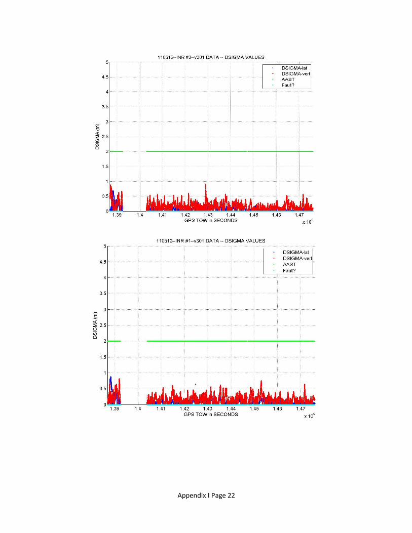
Plots below show the parameters for DSIGMA. Dv and Dl from two INRs run on the same flight are
plotted. There were no DSIGMA monitor failures. The Active Approach Service Type was initially GBAS
GAST D. The aircraft was out of PAR initially. As it moved IN PAR, the CCD monitor acted on both INRs
and they dropped to Autonomous Navigation mode. This is because the CCD filter output for all
measurements was higher than the threshold and it hadn’t passed the 20 minute observation period.
After that period, the receivers went to GAST D mode and dropped only when the aircraft was farther
than Dmax. This plot also shows whether the FD algorithm has found a measurement inconsistency in
the solution. No faults were detected in any flight tests.
Appendix I Page 22
Appendix I Page 23
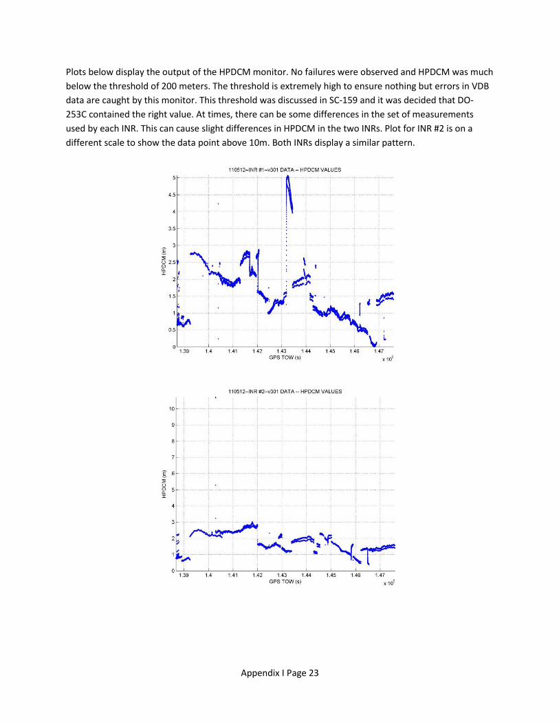
Plots below display the output of the HPDCM monitor. No failures were observed and HPDCM was much
below the threshold of 200 meters. The threshold is extremely high to ensure nothing but errors in VDB
data are caught by this monitor. This threshold was discussed in SC-159 and it was decided that DO-
253C contained the right value. At times, there can be some differences in the set of measurements
used by each INR. This can cause slight differences in HPDCM in the two INRs. Plot for INR #2 is on a
different scale to show the data point above 10m. Both INRs display a similar pattern.

Appendix I Page 24
Plots below show the Lateral Test statistics for the RRFM monitor. Initially, the aircraft is on the ground
and threshold is high to compensate for multipath on ground. No failures were observed on ground or in
air. Three reference receivers were active on this day.

Appendix I Page 25
Plots below show the Vertical Test statistics for the RRFM monitor. Initially, the aircraft is on the ground
and threshold is high to compensate for multipath on ground. No failures were observed on ground or in
air. Three reference receivers were active on this day.
Appendix I Page 26
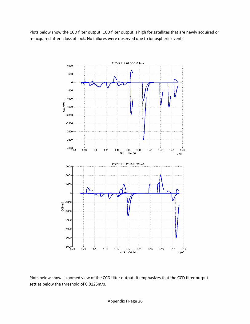
Plots below show the CCD filter output. CCD filter output is high for satellites that are newly acquired or
re-acquired after a loss of lock. No failures were observed due to ionospheric events.
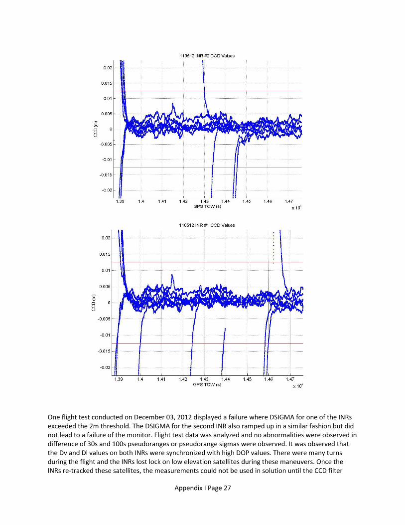
Plots below show a zoomed view of the CCD filter output. It emphasizes that the CCD filter output
settles below the threshold of 0.0125m/s.
Appendix I Page 27
One flight test conducted on December 03, 2012 displayed a failure where DSIGMA for one of the INRs exceeded the 2m threshold. The DSIGMA for the second INR also ramped up in a similar fashion but did not lead to a failure of the monitor. Flight test data was analyzed and no abnormalities were observed in difference of 30s and 100s pseudoranges or pseudorange sigmas were observed. It was observed that the Dv and Dl values on both INRs were synchronized with high DOP values. There were many turns during the flight and the INRs lost lock on low elevation satellites during these maneuvers. Once the INRs re-tracked these satellites, the measurements could not be used in solution until the CCD filter

Appendix I Page 28
output for these measurements was above threshold, so the FD for SV addition algorithm could not allow them to be used in GBAS GAST D mode. Thus, delay in reusing lost measurements due to the high CCD filter output, led to a high DOP. This impacted the DSIGMA values. Following plots display these parameters on both INRs. The CCD filter defined in DO-253C takes a long time to settle. This has quite an impact on availability of satellites that were lost during turns and reacquired later. This monitor along with its impact on DSIGMA will be discussed with RTCA.

Appendix I Page 29
The plots below display the Dl,Dv and active Approach Service type for INR 1 and INR 2. It can be seen that both receivers follow the same pattern. INR1 fails DSIGMA as Dv went as high as 2.04m, while it went to 1.87m on INR2.

Appendix I Page 30
The plots below display the Dl,Dv (in meters) and VDOP for INR 1.
1.41 1.415 1.42 1.425 1.43 1.435 1.44 1.445 1.45 1.455 1.46
x 105
-1
-0.5
0
0.5
1
1.5
2
TOW(s)
DSIGMA INR1
Dl
Dv
1.41 1.415 1.42 1.425 1.43 1.435 1.44 1.445 1.45 1.455 1.46
x 105
0.5
1
1.5
2
2.5
3
3.5
4
4.5VDOP INR1
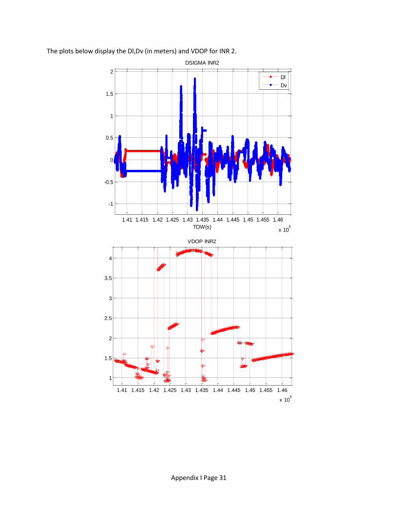
Appendix I Page 31
The plots below display the Dl,Dv (in meters) and VDOP for INR 2.
1.41 1.415 1.42 1.425 1.43 1.435 1.44 1.445 1.45 1.455 1.46
x 105
-1
-0.5
0
0.5
1
1.5
2
TOW(s)
DSIGMA INR2
Dl
Dv
1.41 1.415 1.42 1.425 1.43 1.435 1.44 1.445 1.45 1.455 1.46
x 105
1
1.5
2
2.5
3
3.5
4
VDOP INR2
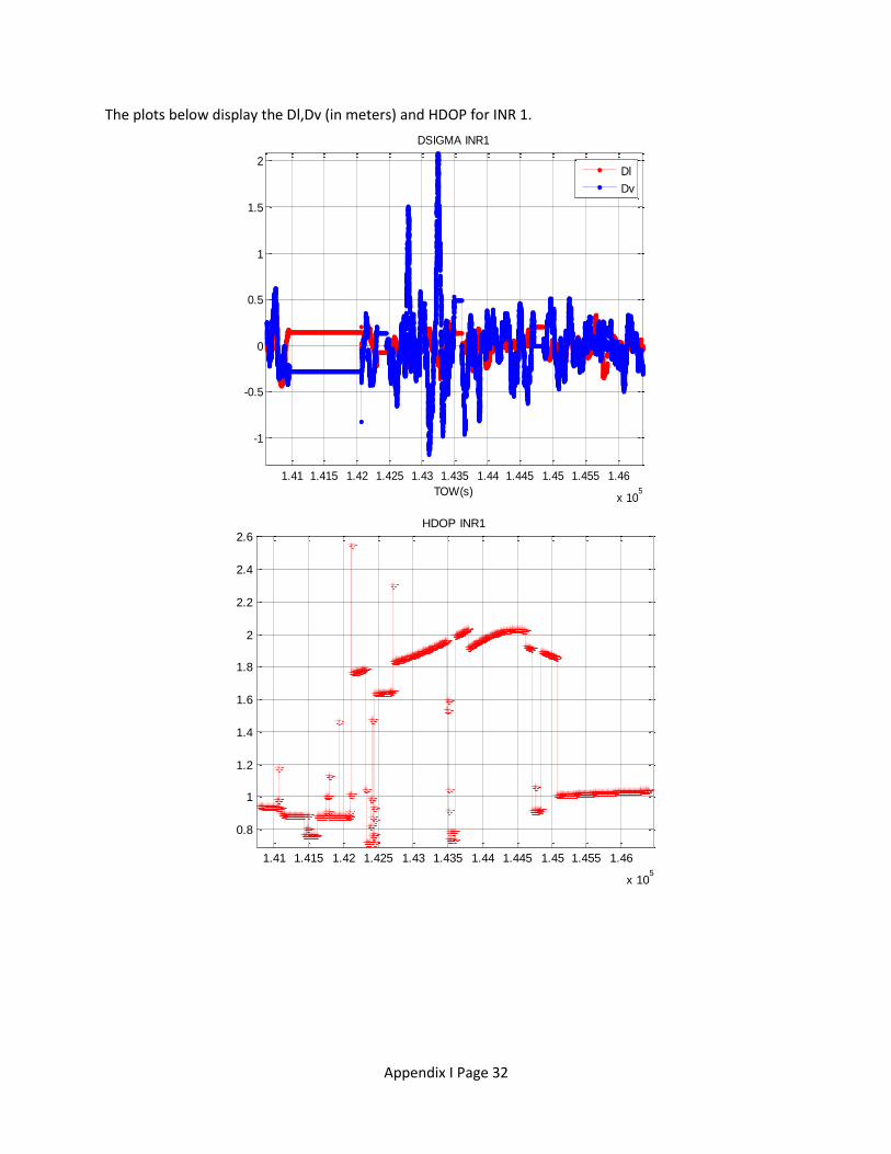
Appendix I Page 32
The plots below display the Dl,Dv (in meters) and HDOP for INR 1.
1.41 1.415 1.42 1.425 1.43 1.435 1.44 1.445 1.45 1.455 1.46
x 105
-1
-0.5
0
0.5
1
1.5
2
TOW(s)
DSIGMA INR1
Dl
Dv
1.41 1.415 1.42 1.425 1.43 1.435 1.44 1.445 1.45 1.455 1.46
x 105
0.8
1
1.2
1.4
1.6
1.8
2
2.2
2.4
2.6HDOP INR1

Appendix I Page 33
The plots below display the Dl,Dv(in meters) and HDOP for INR 2.
1.41 1.415 1.42 1.425 1.43 1.435 1.44 1.445 1.45 1.455 1.46
x 105
-1
-0.5
0
0.5
1
1.5
2
TOW(s)
DSIGMA INR2
Dl
Dv
1.41 1.415 1.42 1.425 1.43 1.435 1.44 1.445 1.45 1.455 1.46
x 105
0.6
0.8
1
1.2
1.4
1.6
1.8
2
2.2
2.4
HDOP INR2
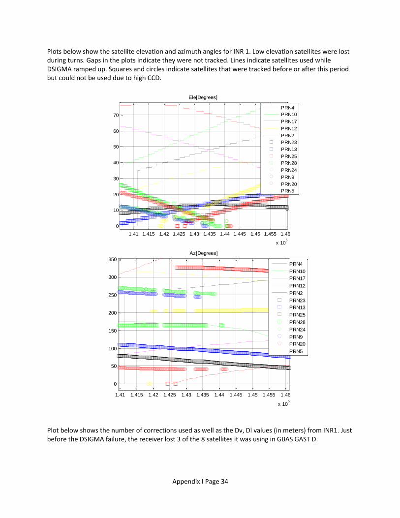
Appendix I Page 34
Plots below show the satellite elevation and azimuth angles for INR 1. Low elevation satellites were lost during turns. Gaps in the plots indicate they were not tracked. Lines indicate satellites used while DSIGMA ramped up. Squares and circles indicate satellites that were tracked before or after this period but could not be used due to high CCD.
Plot below shows the number of corrections used as well as the Dv, Dl values (in meters) from INR1. Just before the DSIGMA failure, the receiver lost 3 of the 8 satellites it was using in GBAS GAST D.
1.41 1.415 1.42 1.425 1.43 1.435 1.44 1.445 1.45 1.455 1.46
x 105
0
10
20
30
40
50
60
70
Ele[Degrees]
PRN4
PRN10
PRN17
PRN12
PRN2
PRN23
PRN13
PRN25
PRN28
PRN24
PRN9
PRN20
PRN5
1.41 1.415 1.42 1.425 1.43 1.435 1.44 1.445 1.45 1.455 1.46
x 105
0
50
100
150
200
250
300
350
Az[Degrees]
PRN4
PRN10
PRN17
PRN12
PRN2
PRN23
PRN13
PRN25
PRN28
PRN24
PRN9
PRN20
PRN5

Appendix I Page 35
1.41 1.415 1.42 1.425 1.43 1.435 1.44 1.445 1.45 1.455 1.46
x 105
0
2
4
6
8
10
TOW[s]
Number of corrections used

Appendix I Page 36
Plot below shows the CCD filter output (in m/s) for satellites tracked by INR1. It can be seen that CCD filter was reset several times for some satellites. This synchronized with the turns. A plot showing change in the ground track is also displayed.
1.42 1.425 1.43 1.435 1.44 1.445
x 105
-250
-200
-150
-100
-50
0
50
100
150
200
CCD[m]
PRN4
PRN10
PRN17
PRN12
PRN2
PRN23
PRN13
PRN25
PRN28
PRN24
PRN9
PRN20
PRN5
1.42 1.425 1.43 1.435 1.44 1.445
x 105
-0.5
-0.4
-0.3
-0.2
-0.1
0
0.1
0.2
0.3
0.4
0.5
Change in ground track

Appendix I Page 37
Appendix A: Evaluation of GBAS fault detection performance
Introduction RTCA/DO-253C, section 2.3.9.6 requires
“For AEC D equipment, when GAST D is active and the aircraft is inside the PAR the PAN shall perform
fault detection on the precision approach position solution based on 30-second smoothing using
redundant corrected pseudorange measurements if more than four satellites with associated differential
corrections are available.
The fault detection algorithm shall be performed at a rate of at least once per minute, as well as within 6
seconds of entering the PAR and within 2 seconds of a satellite geometry change. If a fault is detected,
the equipment shall change the active Approach Service Type to C and output appropriately per section
2.3.11.1.3.3, or use a subset geometry for which the limit is not exceeded.
The probability of missed detection has no requirement. The threshold shall be set to provide a
probability of false alert equal to 10-7 per sample.”
Given a correct implementation of a Fault Detection (FD) algorithm, it is desirable to evaluate how such
an algorithm would operate when confronted with real world conditions. In particular, the intent is to
evaluate the behavior of the algorithm when presented with typical atmospheric conditions and the
behavior when the atmosphere is stimulated into atypical behavior.
This paper presents the approach Honeywell used to examine the characteristics of the GBAS FD
algorithm used in the GNSS Prototype S/W (722-20103-E202). The tests performed to verify the False
Alert rate and Missed detection rate have been discussed in detail. This paper also takes a brief look at
the performance of this algorithm during a set of flight tests performed by the FAA team with a couple
of INRs that were programmed with the GNSS Prototype S/W (722-20103-E202). Finally,
recommendations have been provided for the addition of a detailed test section for the GBAS FD
algorithm, in the RTCA/DO-253 document.
Test framework RTCA/DO-229D, section 2.5.9 presents a methodology for examining the availability, false alert rate and
missed detection probabilities for a Fault Detection (FD) implementation. While acknowledging that the
DO-253 FD requirements do not have specific availability or missed detection probability requirements
except in the case of FD for satellite addition, this methodology provides a good starting point for
examining the behavior of the DO-253 algorithm.
The first portion of the DO-229 testing requires the evaluation of the availability of the FD algorithm
assuming that the probability of missed detection is 0.001 and further assuming certain characteristics
of the residual errors. This evaluation applies over a regularized grid of space-time coordinates.
Following this evaluation, a subset of 40 space-time points is selected which provides a uniform
distribution of protection levels and exclusion levels (0.1 to 4.0 nmi in the case of the INR). This subset is
then used in the evaluation of false alarm rate and probability of missed detection. Because the DO-253

Appendix I Page 38
algorithm has neither availability nor missed detection requirements, this sort of selection is not directly
possible. However, because the INR implements the DO-253 requirements using exactly the same
algorithm as the DO-229 requirements, albeit with different thresholds, using the same subset of
geometries for the GBAS algorithm as for the unaugmented algorithm provides the same desirable
variety in the relative positioning of the satellites.
2.1 PRAIMVT Offline Toolscripting engine
Given the selected satellite geometries, it is then possible to create a simulation in which models of
measurements corrupted with real-world errors can be presented to the FD algorithm. To perform this
simulation, we will adapt the “PVT Scripting Engine”RAIM Offline Tool previously developed for
performing the DO-229 FD verification was adapted.
Operation of the scripting engine this RAIM Offline Tool is shown in Figure 3. A basic description of the
block diagram of the implementation of the PVT Script Engine is shown in Figure 4.
Corrupt
Measurement
Select
Geometries
Precompute
Perfect
Measurements
Model Control
Script Output
Performance
Assessment
Execute PVT
Monitor for Outcome
Complete?
Measurements
No
Yes
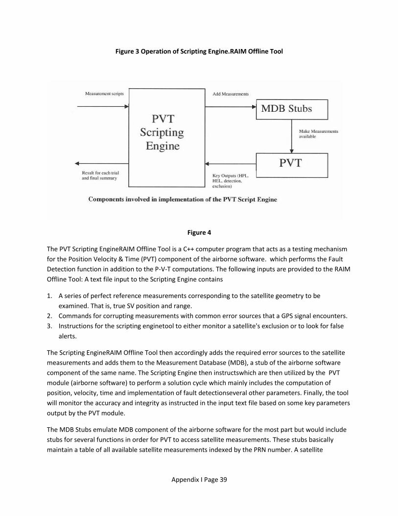
Appendix I Page 39
Figure 3 Operation of Scripting Engine.RAIM Offline Tool
Figure 4
The PVT Scripting EngineRAIM Offline Tool is a C++ computer program that acts as a testing mechanism
for the Position Velocity & Time (PVT) component of the airborne software. which performs the Fault
Detection function in addition to the P-V-T computations. The following inputs are provided to the RAIM
Offline Tool: A text file input to the Scripting Engine contains
1. A series of perfect reference measurements corresponding to the satellite geometry to be
examined. That is, true SV position and range.
2. Commands for corrupting measurements with common error sources that a GPS signal encounters.
3. Instructions for the scripting enginetool to either monitor a satellite's exclusion or to look for false
alerts.
The Scripting EngineRAIM Offline Tool then accordingly adds the required error sources to the satellite
measurements and adds them to the Measurement Database (MDB), a stub of the airborne software
component of the same name. The Scripting Engine then instructswhich are then utilized by the PVT
module (airborne software) to perform a solution cycle which mainly includes the computation of
position, velocity, time and implementation of fault detectionseveral other parameters. Finally, the tool
will monitor the accuracy and integrity as instructed in the input text file based on some key parameters
output by the PVT module.
The MDB Stubs emulate MDB component of the airborne software for the most part but would include
stubs for several functions in order for PVT to access satellite measurements. These stubs basically
maintain a table of all available satellite measurements indexed by the PRN number. A satellite
Appendix I Page 40
measurement generally consists of pseudo-range, range-rate, standard-deviation of the measurement,
and satellite positions.
The PVT component of the airborne software is reused as part of the scripting engine to provide the
position solution and to implement the FD algorithm. Minor modifications may be required to enable
the tool's execution on the Windows platform. Every modification to the PVT software will be reviewed
and tested.
2.2 Components of the scripting engineRAIM Offline Tool
In addition to the components taken from the airborne software and the stubssupporting software
necessary to support executing theat softwaretool in an off-line environment, the scripting engineRAIM
Offline tool consists of a performance monitor as well as a series of measurement models, used to
corrupt the pre-computed reference measurements.
2.2.1 Performance monitor
The performance monitor examines the error in the solution computed by the PVT, the protection level,
FD detection status, Fault Exclusion (FE) status and other parameters to determine if the FD algorithm is
operating correctly. Figure 5 shows the operation of the performance monitor.
In the case of false alert performance checking, the script contains a command that indicates no satellite
failures will appear in the test. Tthe monitor will check after each PVT computation cycle and ensure
that no FD annunciation or fault exclusion takes place. Either condition will result in an output to the
user that a false detection has occurred. The monitor will continue to examine the outputs of the PVT
until the endfor the duration of the test.
When examining missed detection performance, the script contains a command indicatingmonitor is
told which satellite is to exhibit a failure. The monitor will compare the error in the computed position
to the output protection levels as well as the detection and exclusion statuses. It will stop the testThe
test will stop when the monitor detects a correct exclusion, a missed alert or a failed exclusion.
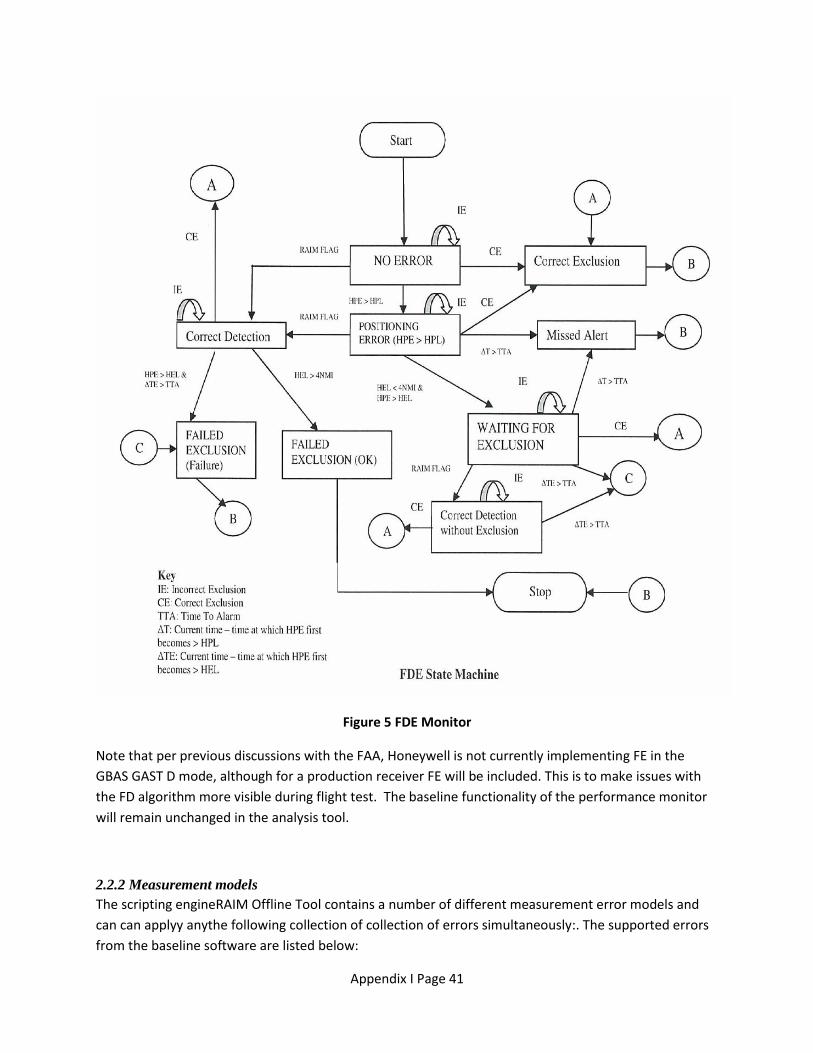
Appendix I Page 41
Figure 5 FDE Monitor
Note that per previous discussions with the FAA, Honeywell is not currently implementing FE in the
GBAS GAST D mode, although for a production receiver FE will be included. This is to make issues with
the FD algorithm more visible during flight test. The baseline functionality of the performance monitor
will remain unchanged in the analysis tool.
2.2.2 Measurement models
The scripting engineRAIM Offline Tool contains a number of different measurement error models and
can can applyy anythe following collection of collection of errors simultaneously:. The supported errors
from the baseline software are listed below:

Appendix I Page 42
Selective Availability, per RTCA/DO-229C, Appendix B.3.
1. Simulated satellite failure, a constant, user specified bias summed with a user specified ramp
error, as either a code or ephemeris bias.
2. Additive White Gaussian Noise, zero mean with user specified standard deviation
3. Receiver Noise, Additive White Gaussian carrier and code terms with user specified standard
deviation.
4. Tropospheric residual, as described below
5. Ionospheric residual, as described below
6. SBAS SFLT errors, first order Gauss-Markov model
7. Multipath, Normal Random Variate with elevation angle dependent standard deviation
meters
8. Satellite Clock/Ephemeris Error, First Order Gauss-Markov
To these we will add
9. Ground Station Errors, as described below
For the purposes of evaluating the GBAS FD algorithm, only the receiver noise, multipath, tropospheric,
ionospheric and ground station error models will be employed. For the missed detection tests, the ramp
error function will also be Theutilized. The following sections describe these errors in more detail.
2.2.3 Ionospheric residuals
The ionospheric residual can be modeled in a variety of ways depending on the needs of the simulation.
For unaugmented measurements, the residual can be taken as the whole ionosphere delay computed
using the IRI 2001 ionosphere model developed by NASA (http://iri.gsfc.nasa.gov/). Note that newer
versions of this model exist, but the scripting engine handles only up through the 2001 release.
Alternatively, the ionospheric residual can be simulated as a first order Gauss-Markov model with
variable mean and correlation time parameters.
Honeywell used the following algorithm to simulate the ionospheric residual forFor GBAS
measurements, the ionospheric residual is simulated using the following .algorithm (refer Appendix A
for more details)
1. For each iteration of the simulation, select a gradient, g, as a sample from the exponential
distribution

Appendix I Page 43
where is user selectable as either 1.65755 mm/km or 13 mm/km as described in Dautermann et al.
and Belabbas et al. respectively. Note that each iteration of the simulation has a duration of 20 minutes
in an effort to simulate a single approach.
2. For each iteration, select a random airport position relative to the user position. That is, select
to be a random variate selected from uniform distribution over the range [0 10 nmi].
Also, select an aircraft velocity as a random variate from a uniform distribution over the
range [100 250 knots].
A higher range can be selected and this could lead to higher residuals but note that the
standard deviation for iono residual error would also be equivalently inflated.
3. Given the gradient from step 1, the ionospheric residual, , of each satellite is computed
as
Where
Note that the same gradient is used for all satellites for the duration of a given simulation iteration,
however, the specific error applied to each satellite will depend on its elevation angle.
The transmitted is assumed to be a fixed 6.4 mm/km as this is the term broadcast by
the Honeywell SLS ground stations. While, it is acknowledged that this value may vary with satellite
geometry, for the purposes of this test, it is assumed as a constant.
2.2.4 Tropospheric residuals
The tropospheric residual can take on one of three forms.
For unaugmented measurements, the troposphere residual is taken from a first order Gauss-Markov
process with a mean of 0, a standard deviation of 1.0 meter and a correlation time of 20 seconds. The
weight used in the PVT and FD algorithms is given by .
Alternatively, for SBAS augmented measurements or unaugmented measurements while testing per DO-
229D, the troposphere residual is taken as a random constant with a standard deviation given by
. The weight used in the PVT and FD algorithms is the same .

Appendix I Page 44
For GBAS measurements, the tropospheric residual is once again taken as a random constant with a
standard deviation given by
Where:
is the computed satellite elevation angle
h is the computed difference in altitude between the GNSSA antenna and the ground
subsystem altitude received in the Type 2 message in meters
h is the troposphere scale height received from the ground subsystem in Type 2 message in
meters
is the refractivity uncertainty (unitless) received from the ground subsystem in Type 2
message
The values for h and were determined by examining pressure, temperature, and relative humidity
measurements taken at hourly intervals at different airports. Scale height and refractivity uncertainty
were computed based on these measurements and the yearly average is now being broadcast as shown
below. For the purposes of simulation, the scale height will be taken from a normal distribution with a
mean of 15600 meters and a standard deviation of 800 meters. The refractive uncertainty will be taken
from a normal distribution with a mean of 18 and a standard deviation of 5. These values will be the
same for all satellites and will remain constant for the duration of the simulation.
Sample Tropo
Parameters
Refractivity
Index
Scale
Height
Refractivity
Uncertainty
Installation (unit-less) (m) (unit-less)
Bremen 328 16100 11
Houston 349 14300 25
Malaga 334 15100 17
Newark 325 16300 20
Rio 325 16300 20
Sydney 325 15600 16
MIN 325 14300 16

Appendix I Page 45
MAX 349 16300 25
MEAN (μ) 331 15616 18.2
STANDARD
DEV.(σ)
9.5 796 4.7
2.2.5 Ground station errors
Testing was performed at several Honeywell GBAS ground station installations and typical values of
smoothed range residual and broadcast were collected for each reference receiver. Analysis of
this data indicates that Testing was performed at Moses Lake and typical values of smoothed range
residual and broadcast were collected for each reference receiver. Figure 6 and Figure 7 show
these observations as a function of satellite elevation angle. For elevations above 5 degrees, the sigma
PR Ground values must be within 0.05 to 0.10 m. The 5 degree elevation may exceed 5cm in order to
avoid sigma events. The SLS-4000 continuously monitors real-time sigma (measurement variance)
against the nominal sigmas within the MSD file. If the real-time sigmas regularly exceed the nominal
values, a [RR/SV] measurement, RR, or the entire system will be excluded.

Appendix I Page 46
Figure 6
Results from tests at Newark, Sydney and Bremen were very similar and so the following model has
been chosenthe residual error contribution by the ground station can be modeled as a random error
generated from a Normal distribution with the standard deviation computed as shown below.:
Modeled Equation for σpr_gnd (used to generate residual errors (mean = 0))
Random errors will be generated from a Normal distribution with the standard deviation computed as
shown above. Note that this expression assumes, based on DO-253C requirement, LAAS-316, that
.

Appendix I Page 47
Figure 7
Results from tests at Newark, Sydney and Bremen were very similar and so tAnalysis of the broadcast
values indicates that the following values can be chosen to emulate the values
broadcast in Type 1 Message. For the purposes of FD verification in GASTD mode, these same values
have been used to emulate the values transmit in Type 11 messages.he following model has
been chosen.
Model for Broadcast σpr_gnd values
Note that this expression assumes, based on DO-253C requirement, LAAS-316, that . Also, note
that this model emulates the values broadcast in Type 1 Message and used for the GASTC
mode. However, for the purposes of FD verification in GASTD mode, the same model has been used to
emulate the values transmit in Type 11 messages.

Appendix I Page 48
3. Selection of simulation parameters for the False Alert Rate Test
According to DO-229D, Section 2.5.9.4, verifying a false alert rate of 3.33e-7 per sample for the FD
algorithm, requires the simulation of hours of flight time. This time is spread across each of
the 40 geometries identified in section 1. This means that each location will receive
hours of simulation. Note that DO-229D allows 47 false alerts over this simulation period for
testing a PFA of 3.33e-7 with the desired statistical confidence as provided in section 2.5.9.4 of DO-
229D. It can hence be inferred that, to test the PFA of 1e-7 required for the GBAS FD algorithm, either a
longer simulation time would be needed or a lower number of false alerts would be allowed. Honeywell
has chosen to run the GBAS False Alert test with the same simulation time and then make a Pass/Fail
determination based on the number of false alerts observed. Note that if the False Alert test for the
GBAS FD algorithm is added to the MOPS, the exact number of allowed false alerts would have to be
determined based on the desired statistical confidence.
For the GBAS FD test, the 82500 hours of simulation time for each geometry are further broken into 20
minute approaches, each of which will have its own unique airport location and aircraft velocity. Each
simulation will be commanded to apply the following corruptions to each satellite measurement:
1. Receiver noise
2. Multipath
3. GBAS tropospheric residuals
4. GBAS ionospheric residuals
5. GBAS ground station residuals
Two separate sets of simulation will be performed. The first set is intended to represent nominal
atmospheric conditions. In this data set, the ionospheric residual model will select a gradient from the
exponential distribution in section 0 2.2.3 with . as chosen by Dautermann et al.
The second set of simulations is intended to represent an atypical atmospheric condition. In this data
set, the ionospheric residual model will select from the exponential distribution in section 0 2.2.3 with
as described by Belabbas et al.
4. Test Observations and Results
4.1 False Alert Rate Tests
Two separate sets of simulations were executed as a part of the False Alert Rate tests. The first set
included the nominal ionospheric residual (Dautermann model) model and the second set included the
atypical ionospheric residual (Belabbas model) model. All error models listed in section 3 were enabled
to corrupt the measurements.
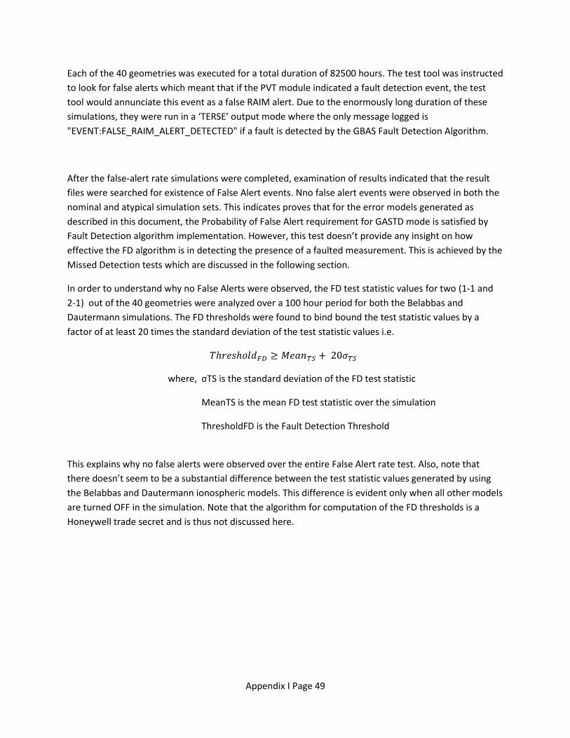
Appendix I Page 49
Each of the 40 geometries was executed for a total duration of 82500 hours. The test tool was instructed
to look for false alerts which meant that if the PVT module indicated a fault detection event, the test
tool would annunciate this event as a false RAIM alert. Due to the enormously long duration of these
simulations, they were run in a ‘TERSE’ output mode where the only message logged is
"EVENT:FALSE_RAIM_ALERT_DETECTED" if a fault is detected by the GBAS Fault Detection Algorithm.
After the false-alert rate simulations were completed, examination of results indicated that the result
files were searched for existence of False Alert events. Nno false alert events were observed in both the
nominal and atypical simulation sets. This indicates proves that for the error models generated as
described in this document, the Probability of False Alert requirement for GASTD mode is satisfied by
Fault Detection algorithm implementation. However, this test doesn’t provide any insight on how
effective the FD algorithm is in detecting the presence of a faulted measurement. This is achieved by the
Missed Detection tests which are discussed in the following section.
In order to understand why no False Alerts were observed, the FD test statistic values for two (1-1 and
2-1) out of the 40 geometries were analyzed over a 100 hour period for both the Belabbas and
Dautermann simulations. The FD thresholds were found to bind bound the test statistic values by a
factor of at least 20 times the standard deviation of the test statistic values i.e.
where, σTS is the standard deviation of the FD test statistic
MeanTS is the mean FD test statistic over the simulation
ThresholdFD is the Fault Detection Threshold
This explains why no false alerts were observed over the entire False Alert rate test. Also, note that
there doesn’t seem to be a substantial difference between the test statistic values generated by using
the Belabbas and Dautermann ionospheric models. This difference is evident only when all other models
are turned OFF in the simulation. Note that the algorithm for computation of the FD thresholds is a
Honeywell trade secret and is thus not discussed here.

Appendix I Page 50
4.2 Missed Detection Tests
The DO-253 FD requirements do not have specific availability or missed detection probability
requirements. Honeywell suggests the addition of Missed Detection tests on the lines of the SBAS
Missed Detection tests (DO-229, Section 2.5.10) to the RTCA/DO-253. These tests involve the
computation of a VPLTFD term assuming a missed detection probability of 0.1. Honeywell also has
additional recommendations with regards to verification of the FD algorithm and they are discussed in
Section 7 of this document. For the purposes of this program, a Missed Detection test was executed for
GBAS FD implementation and its methodology has been explained below.
The test tool (PVT Scripting EngineRAIM Offline Tool) was modified to compute the VPLTFD term and the
performance monitor was instructed to annunciate a missed alert if the vertical position error exceeded
the VPLTFD and, no fault was detected by the PVT module within the next 4s (Time To Alarm: TTA). The
RAIM Offline Tool PVT Scripting Engine was also set-up to terminate execution if a fault-detection or a
missed-alert was observed.
The RAIM Offline Tool PVT Scripting Engine was then executed with the same set of 40 geometries and
same set of error models that were used for the False Alert Rate tests. In addition, a pseudorange ramp
error (0.02 m/s) was added to the hardest to detect measurement (along the vertical direction) for each
geometry. For all the 40 geometries, these simulations were executed 14 times with a different random
number seed every time. This ensured that a different set of measurement error values were presented
to the PVT module in each simulation. Note that the SBAS Missed Detection tests in Section 2.5.10 of
DO-229D require only 20 geometries to be executed for 14 times each to test the if PMD <= 0.1
requirement. There is no missed alert probability for the SBAS FD algorithm but a test has been specified
in Section 2.5.9.4 of DO-229D in order to gauge the effectiveness of this algorithm.
After all the simulations were completed, the result files were collected and analyzed. It was confirmed
that at all 40 geometries were run 14 times and that there were no missed alerts. Note that the SBAS
Missed Detection tests in RTCA/DO-229(), Section 2.5.10.3.3 allow up to 40 alerts over admissible
geometries while none were encountered here, so the test passed. This indicates that the GBAS FD
algorithm was effective in identifying the existence of faulted measurements. This also concludes that
the probability of missed detection of the implemented GBAS FD algorithm is lower than 0.1.
5. Flight-Test Analysis
Two sets of flight tests were performed and analyzed for the behavior of the Fault Detection algorithm
in GASTD modes. These flight tests included approaches flown against both the LTP and the SLS-4000
ground stations at Atlantic City Airport (KACY). The observations from these flight tests are summarized
below.
On 20th, 21st, 24thand 25th January 2012, flight tests were performed by the FAA team with two
Honeywell Integrated Navigation Radios (INR) onboard. These INRs were programmed with GNSS

Appendix I Page 51
Prototype S/W build E200 (p/n: 722-20103-E200) and their outputs were collected during the flight test.
The collected data was later analyzed and the following observations were made. (Note that none of the
GASTD specific monitors were activated in build E200.)
• Two FD events were observed in air (one against the SLS and one against the LTP). Data
indicated high residuals on a measurement that had also failed the CCD monitor. So, the FD
algorithm behaved as expected.
• Few FD events were observed with the LTP and they were co-incident with D-sigma spikes that
can be attributed to spikes in Range-rate correction term transmitted by the LTP. This is a known
issue with the LTP and a known defect in the GNSS software which was fixed in the next update.
Tthe FD algorithm however, had behaved as expected.
• Several FD events were observed on ground due to multipath (These events were expected).
Note that the INR implements a ground-based multipath model when the aircraft is on the
ground and static (or moving very slowly). While this ground-based multipath model does inflate
measurement variances substantially, it doesn’t adequately bounind the multipath errors at all
times.
• Analysis of the available flight-test data indicates that activation of the FD algorithm should
provide the necessary integrity monitoring. Activation of CCD monitors can reduce the number
of FD events observed. It can be concluded that no False Alerts were observed.
Another set of flight tests were performed in May 2012 by the FAA team with two INRs onboard. One
INR was programmed with GNSS Prototype S/W build E201 (p/n: 722-20103-E201) and the other was
programmed with GNSS Prototype S/W build E202 (p/n: 722-20103-E202). The data from these flight-
tests was collected and analyzed. Three FD events were observed and they were all on-ground. FD
events on the ground are expected and can be attributed to multipath. So, here again, it can be
concluded that the FD algorithm behaved as expected as there were no False Alerts.
6. Conclusion
The GNSS prototype S/W E202 (p/n: 722-20103-E202) implemented a Fault Detection algorithm in
GASTD and GASTC modes, according to the specifications in Section 2.3.9.6 of RTCA/DO-253C. This
implementation was then verified through a combination of (PC-based) offline testing and flight-tests.
The offline testing was based on a methodology very similar to the existing tests for Un-augmented FD
(DO-229D, Section 2.5.9) and SBAS FD (DO-229D, Section 2.5.10) algorithms. Models for residual errors
encountered in GBAS were generated and utilized for the offline testing. False Alert tests were
performed and it was verified that the GBAS FD implementation had a probability of False Alarm (PFA)
lower than 1e-7. Missed detection tests were also performed and it was verified that the FD
implementation had a probability of missed alert lower than 0.1. Additionally, the analysis of data
collected during flight-tests proved that there were no unexpected FD events. Based on all these tests, it

Appendix I Page 52
can be concluded that the GNSS Prototype S/W E202 satisfies the Fault Detection requirements
specified in RTCA/DO-253C, Section 2.3.9.6.
7. Future work
Honeywell recommends the addition of a GBAS Fault Detection test section to RTCA/DO-253C. This
section should be modeled on section 2.5.10 of RTCA/DO-229D and ideally should detail the following:
1) GBAS Residual Error Models
This section should specify the models that need to simulate the GBAS residual errors. The models
discussed in Section 2.0 of this document or other appropriate models can be specified.
2) GBAS Availability Test
This test can be modeled similar to the Availability tests specified for SBAS (Section 2.5.10.2, RTCA/DO-
229D). A VPLTFD term can be computed for test purposes and an appropriate VAL can be chosen for the
availability tests. A required availability percentage can also be specified.
3) Geometry Selection
This section should explain the basis of geometry selection and LGF position selection.
4) GBAS False Alert Rate Test
This test can be modeled similar to Section 2.5.10.4 of RTCA/DO-229D or Section 4.1 of this document.
The exact duration of simulation needs to be specified based on the desired statistical confidence for
the Probability of False Alert value.
5) GBAS Missed Detection Test
This test can be modeled similar to Section 2.5.10.3.3 of RTCA/DO-229D or Section 4.2 of this
document. The number of trials of the test for all geometries should be finalized depending on the
desired Probability of missed detection.
6) On-Line Verification Tests
These tests can be modeled similar to Section 2.5.10.5 of RTCA/DO-229D.
7) FD for SV Addition
Tests for Missed Detection and False Alert probabilities of the FD for SV Addition algorithm should also
be specified. The offline tool can be used for these tests but would need some additional capability.
8. Bibliography
1) Belabbas, B., Dautermann, T., Looye, G., & Kladetzke, J. (2010). GBAS Based Autoland System: A
Bottom Up Approach for GAST-D Requirements. Position Location and Navigation Symposium
(PLANS), 2010 IEEE/ION, (pp. 566-574). Indian Wells, CA.
2) Dautermann, T., Mayer, C., Antreich, F., Konovaltsev, A., Belabbas, B., & Kalberer, U. (2012).
Non-Gaussian Error Modeling for GBAS Integrity Assessment. IEEE Transactions on Aerospace
and Electronic Systems , 693-706.
3) Minimum Operational Performance Standards For Global Positioning System/Wide Area
Augmentation System Airborne Equipment, RTCA/DO-229D

Appendix I Page 53
4) Minimum Operational Performance Standards For GPS Local Area Augmentation System
Airborne Equipment, RTCA/DO-253C
5) Christie, J. R., Ko, P.-Y., Hansen, A., Dai, D., Pullen, S., Pervan, B. S., et al. (1999). The Effects of
Local Ionoshperic Decorrelation on LAAS: Theory and Experimental Results. ION NTM-99. San
Diego.
6) Mayer, C., Jakowski, N., Borries, C., Pannowitsch, T., & Belabbas, B. (2008). Extreme ionospheric
conditions over Europe observed during the last solar cycle. NAVITEC 2008.
7) Pervan, B., Pullen, S., Andreacchi, & Enge, P. (2000). Characterizing the Effects of Ionospheric
Divergence and Decorrelation on LAAS. ION GPS 2000, (pp. 653-661). Salt Lake City.
8)
Appendix B: Ionospheric Model for GBAS Test Data Generation
1. PDF for Ionosphere Gradient
Christie (Christie, et al., 1999) first reported on an examination of ionospheric data for the calendar year
1998, with results suggesting that hourly ionospheric measurements exhibited an exponential
probability density function. Subsequent results reported by Pervan (Pervan, Pullen, Andreacchi, &
Enge, 2000) for data during two ionospheric storms in 2000 showed similar exponential behavior.
Mayer (Mayer, Jakowski, Borries, Pannowitsch, & Belabbas, 2008) examined data from 2000-2008 for
GPS receivers located in Europe and again observed data distributions that exhibited exponential
behavior. The mathematical form for such a distribution when properly normalized is
where g is the gradient in mm/km and is an appropriate scaling factor. Relying on the results reported
by Mayer (Mayer, Jakowski, Borries, Pannowitsch, & Belabbas, 2008), Belabbas et al. (Belabbas,
Dautermann, Looye, & Kladetzke, 2010) have used a value of = 13 in reported efforts to characterize
the performance of a GBAS system in GAST-D mode. That data set included observations made over
latitudes from 20 N to 90 N. Mayer et al. (Mayer, Jakowski, Borries, Pannowitsch, & Belabbas, 2008)
present plots that show that most gradients above 50 mm/km occur in the equatorial and polar regions,
whereas mid-latitudes from 30 -60 produce very few gradients that large. Hence, the Mayer data and
the resulting Belabbas value for would represent a very conservative choice. Dautermann et al.
(Dautermann, Mayer, Antreich, Konovaltsev, Belabbas, & Kalberer, 2012) employed a reduced set of
measurements for the dates October 1-9, 2003, when ionosphere disturbances were low to moderate
and solar activity was moderate. Their argument for restricting attention to more modest levels of
ionospheric disturbances is that larger amounts of ionospheric disturbance would be identified and

Appendix I Page 54
excluded from use by the monitors in the GBAS ground station and the aircraft receiver. The value of
they elected to use was =1/0.6033 = 1.65755 mm/km.
Honeywell proposes to begin the testing effort with the lower value for proposed by Dautermann et
al., and reserve the more conservative value proposed by Belabbas et al. for subsequent rounds of
testing. This should prove reasonable for assessing performance over the contiguous United States,
while the more conservative value might be required for evaluation of airports located in equatorial
regions below 30 latitude and polar regions above 60 latitude.
2. Temporal changes in the ionospheric gradient
If the ionosphere were spatially uniform and maintained a fixed TEC (Total Electron Count), there would
be very little residual iono contribution to the pseudorange. Spatial variations in the TEC can be
reasonably expected, and the use of the exponential distribution allows us to include their effect up to a
degree. It is entirely reasonable to expect that there will be gradients and that these gradients will not
maintain a fixed location relative to the earth. Instead, we can expect that these gradients will appear
to move and change with time. Various monitors on the ground and aboard the aircraft are intended to
recognize the arrival of a large gradient and to remove the relevant satellites from service. But there
will still be temporal changes in the gradient that would result in an additional contribution to the
pseudorange error. Each approach event Honeywell needs to simulate for testing purposes extends
over a period of 20 minutes. A total of 247,500 approaches for a total of 82,500 hours of testing will be
performed for each of 40 geometries. For initial testing efforts, Honeywell will pick a random value for
the gradient at the start of each approach trial, keep it fixed until that approach is complete and select a
new value for the next trial. Note that other geometry related aspects that factor into the pseudorange
residual will produce changing results during each approach, but the gradient itself will be held constant.
The opportunity exists to have the gradient change over the course of the approach, at levels that would
not trigger a monitor. Dautermann et al. (Dautermann, Mayer, Antreich, Konovaltsev, Belabbas, &
Kalberer, 2012) describe a correlation transfer process that can assure that the gradients still exhibit an
exponential probability density function while a temporal correlation is introduced to the sequence of
gradient values that would be used during each approach. Additional effort is underway at Honeywell
to evaluate whether this additional refinement of the model is called for or if it is sufficient to leave the
gradient constant over the course of the approach.
3. Production of Ionospheric Gradients with an exponential density function
We need to produce values for the ionospheric gradient that would behave as if they were drawn from a
stochastic process that obeyed an exponential probability distribution. When non-Gaussian
distributions are required, one way to accomplish this is to use a technique that relies on a random
number generator that produces values that are uniformly distributed from 0 to 1. For desired densities
such as the exponential distribution that has a nice analytic form for the associated cumulative
distribution function, the inverse of the cumulative distribution can be used to map the uniformly
distributed random values produced by the random number generator in software into a set of random
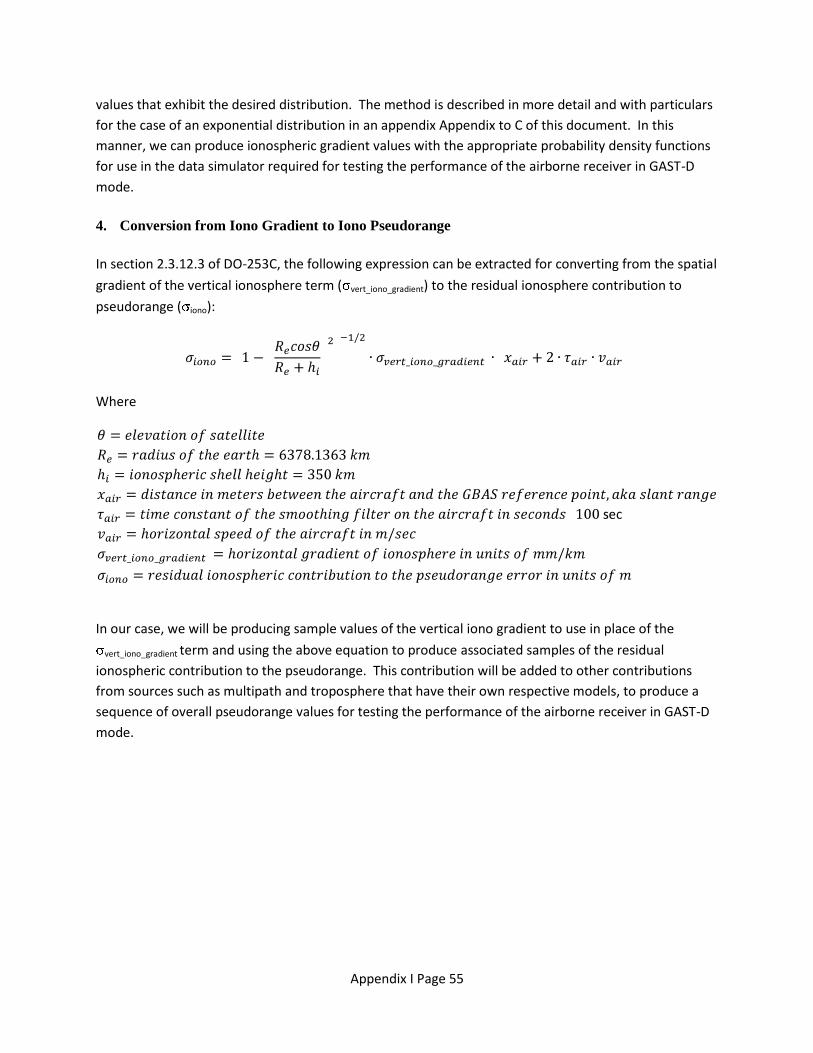
Appendix I Page 55
values that exhibit the desired distribution. The method is described in more detail and with particulars
for the case of an exponential distribution in an appendix Appendix to C of this document. In this
manner, we can produce ionospheric gradient values with the appropriate probability density functions
for use in the data simulator required for testing the performance of the airborne receiver in GAST-D
mode.
4. Conversion from Iono Gradient to Iono Pseudorange
In section 2.3.12.3 of DO-253C, the following expression can be extracted for converting from the spatial
gradient of the vertical ionosphere term ( vert_iono_gradient) to the residual ionosphere contribution to
pseudorange ( iono):
Where
In our case, we will be producing sample values of the vertical iono gradient to use in place of the
vert_iono_gradient term and using the above equation to produce associated samples of the residual
ionospheric contribution to the pseudorange. This contribution will be added to other contributions
from sources such as multipath and troposphere that have their own respective models, to produce a
sequence of overall pseudorange values for testing the performance of the airborne receiver in GAST-D
mode.

Appendix I Page 56
Appendix C: – Creating exponentially distributed samples from random
numbers that are uniformly distributed The starting point for generating the sample values of the ionospheric gradient is a random number
generator that produces uniformly distributed random numbers. Honeywell has a special, extended
version of such a random number generator that ensures uncorrelated behavior over very large
numbers of samples, in order to ensure no unintended correlations are introduced. The method for
producing random samples with a desired, non-uniform probability density, such as the exponential
density, relies on the analytic form of the desired probability distribution function. Recall, the
probability distribution function (also known as the cumulative distribution function or CDF) is the
integral of the probability density function. The CDF has values that fall in the range [0,1]. The method
exploits this fact, applying the inverse of the CDF function to map uniformly distributed random number
into values that exhibit the desired density function. This process is illustrated below for the case of an
exponential distribution.
1. Conversion of uniformly distributed random numbers into exponentially distributed values
The expression for the density function for an exponentially-distributed random variable is
ex
xp/
2
1)(
The associated cumulative distribution function is
02
1 /xfore
x
02
11
/xfore
x
This cumulative distribution function has an easily computed inverse in analytic form given by
If we rely on a uniformly distributed random number generator that produces values y that are in the
interval [0,1], we can compute P-1(y) using the above definition to produce a result that will be
exponentially distributed.
2. Particular case of the FAA simulation
From the papers by Belabbas et al. (Belabbas, Dautermann, Looye, & Kladetzke, 2010)and Dautermann
et al. (Dautermann, Mayer, Antreich, Konovaltsev, Belabbas, & Kalberer, 2012), the desired probability
distribution for the ionospheric gradient is

Appendix I Page 57
In order for this expression to be equivalent to the p(x) expression above for the exponential
distribution, we must set ln(10), where is the multiplicative inverse of the slope obtained from
the logarithmic plot of the estimated probability density function obtained from the histogram of values
that were observed from historical ionospheric data. In the case of Belabbas et al., = 13, while for
Dautermann et al., = 1/0.6033 = 1.65755.
Whichever value of we use, the recipe then becomes the following. Obtain a uniformly distributed
random value in the range [0,1] and use it as input into the following function:
The output of this function will be a random value that has the required exponential distribution, which
is the result we need.
Appendix I Page 58
List of Acronyms
ARINC Aeronautical Radio, Incorporated
CAT Category
DPS Differential Positioning Service
EDAC Error Detection and Correction
EFIS Electronic Flight Instrument System
EGPWS Enhanced Ground Proximity Warning System
FAA Federal Aviation Administration
GAST Generic Automatic Software Test
GBAS Ground Based Augmentation System
GLS Global Location System
GNSS Global Navigation Satellite System Sensor
GPS Global Positioning System
ILS Instrument Landing System
INR Integrated Navigation Radio
LAAS Local Area Augmentation System
LTP LAAS Test Prototype
MMR Multi-Mode Receiver
NASA National Aeronautics and Space Administration
PAR Precision Approach Region
PRC Pseudorange Correction
PVT Position, Velocity, and Time
RAIM Receiver Autonomous Integrity Monitor
RRC Range Rate Correction
RRFM Reference Receiver Fault Monitor
RTCA Radio Technical Commission for Aeronautics
SATNAV Satellite Navigation
TERPS Terminal Procedures or Instrument Approaches
TSO Technical Standard Order
VDB VHF Data Broadcast
VHF Very High Frequency
VOR VHF Onmni-directional Receiver