game theory and economics prof. dr. debarshi das...
TRANSCRIPT
Game Theory and Economics
Prof. Dr. Debarshi Das
Department of Humanities and Social Sciences
Indian Institute of Technology, Guwahati
Module No. # 04
Mixed Strategy Nash Equilibrium
Lecture No. # 01
Mixed Strategy Nash Equilibrium: Introduction
Keywords: Mixed strategy Nash equilibrium, stochastic stead state, Bernoulli payoff
function, von Neumann Morgenstern preference
Welcome to first lecture of module 4 of this course, called Game Theory and Economics. We
are starting with a new topic in this lecture. This topic is called mixed strategy Nash
equilibrium.
(Refer Slide Time: 00:25)
To understand what is mixed strategy Nash equilibrium, let us try to recall what was the basic
idea of Nash equilibrium. The idea, that we have developed and discussed so far, was that
when there are a set of players and these players are taking actions, a Nash equilibrium is a
situation where a player’s action is optimal, given the actions taken by other players.
Now when I am talking about one player is taking an action, which is optimal, it is not the
case that this person is taking action once in a life time and that is the end of it. If that is the
case, if the game was played just once, then a player has no way to understand what actions
are going to be taken by other players. It is because, if you remember, the game is a
simultaneous move game. So, in the game, the actions are taken simultaneously. And if the
actions are being taken simultaneously, a player cannot know beforehand whether a particular
action is his optimal or not optimal.
(Refer Slide Time: 02:34)
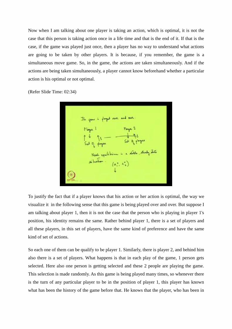
To justify the fact that if a player knows that his action or her action is optimal, the way we
visualize it in the following sense that this game is being played over and over. But suppose I
am talking about player 1, then it is not the case that the person who is playing in player 1's
position, his identity remains the same. Rather behind player 1, there is a set of players and
all these players, in this set of players, have the same kind of preference and have the same
kind of set of actions.
So each one of them can be qualify to be player 1. Similarly, there is player 2, and behind him
also there is a set of players. What happens is that in each play of the game, 1 person gets
selected. Here also one person is getting selected and these 2 people are playing the game.
This selection is made randomly. As this game is being played many times, so whenever there
is the turn of any particular player to be in the position of player 1, this player has known
what has been the history of the game before that. He knows that the player, who has been in

player in 2's position, has been playing a certain action. And the person, who has been in
player 1's position, has been playing a particular action. And these actions are stable.
Stable, in the sense, that they are remaining the same – steady state kind of actions. Now, two
actions – a pair of actions – can be steady state, they can remain the same, only if they are
optimal to each other. Otherwise, if A is not optimal with respect to B, in the next play of the
game, the player who is responsible for A action will change his action because that is not
optimal, given that the other player is playing B.
That is why we say that Nash equilibrium is a stable steady state situation: given the same
pair of action is being played over and over again…so suppose this is the Nash equilibrium –
this pair of action which has been played before and since this has been played before,
whenever player 1 comes to play this action or the player who is in player 1's position comes
to play this action, he knows that player 2 is going to play a2 star. And since he knows that a2
star is going to be played, his optimal is a1 star.
He continuous to play a1 star and the same logic holds for player 2 or whoever the player is in
player 2's position. That is why we say that Nash equilibrium is a stable steady state outcome.
Now, this was the case so far. In mixed strategy Nash equilibrium, what we shall do is that we
are going to change the story a little bit and make it a more generalized case. Generalized
case, in the sense, that here, in mixed strategy Nash equilibrium for any particular player, it is
not the case that his action, a particular action, remains the same. But the pattern of actions
will remain the same. What is meant by pattern of actions?

(Refer Slide Time: 07:11)
Suppose a set of actions of player 1 – a1 a2 am. In Nash equilibrium, what he has been doing is
he was taking this particular action, which is ak star. So ak star is a part of the Nash
equilibrium profile.
Now, ak star is going to be played again and again and the same action is being repeated by
player 1. Instead of that, can we generalize it and say that it is not the case that ak star is going
to be played by player 1 again and again. But what he is going to do is that his probability
distribution over the action set is going to be constant. It is not that the action is remaining
constant but the chances that the actions have of being played will remain constant.
It may happen that player 1 has this action set – a1 and a2. These are the two actions. It’s not
that a1 is going to be played but suppose a1 is going to be played with probability 1/3 and a2
is going to be played with probability 2/3. And these probabilities are going to remain
constant.
If they remain constant for each player, whatever the probabilities are for each player, then
we call that a Nash equilibrium. It is a generalized concept. It is generalized in the sense that I
can have the probability to be 1 and 0 also. In that case, I get back the original concept of
equilibrium – the concept of equilibrium that we have been discussing so far – where one
action is going to be played again and again.

The concept of equilibrium that we have discussed so far is a special case of this generalized
idea of Nash equilibrium, where the pattern of actions, the probabilities that the actions have
in a particular play of the game to be played, those probabilities remain the same. So that is
the general case. The fact that a particular action is going to be played with probability 1, that
is the special case of the generalized case.
So. this is the idea of mixed strategy Nash equilibrium. What we are going to do now is that
this idea of Nash equilibrium or mixed strategy Nash equilibrium can be interpreted in this
way that I have just said – that a particular player attaches suppose probability one-third to
his first action and two-third to the second action, he has only these two actions. This can also
be interpreted in the following way that this population of player 1… out of it, one third of
the population…
So, this is an alternative interpretation of the mixed strategy Nash equilibrium. I have not
rigorously defined what is mixed strategy Nash equilibrium so far. I am just motivating the
idea. This is the alternative idea of mixed strategy Nash equilibrium. If you remember player
1 – the identity of player 1 does not remain constant – the person, who is being played… who
is playing the game in place of player 1, is selected randomly from a population.
Instead of saying that this player, who is playing the game in place of player 1, is playing a1
with one-third and a2 with two-third, we can also say that of the total population behind
player 1, one-third of that population is playing a1 with certainty, and two-third of the
population is playing a2 with certainty.
In this case, since the players are being picked up randomly from the population, the
probability that a1 will be played, remains one-third, and the probability that to a2 is going to
be played is two-third.
So, there are two ways to look at the fact that players are not taking any action for certainty,
but …what is known as randomizing. So this is called randomization. Instead of playing any
action for certainty, a player can be allowed to attach a probability less than one to a
particular action.
(Refer Slide Time: 14:01)
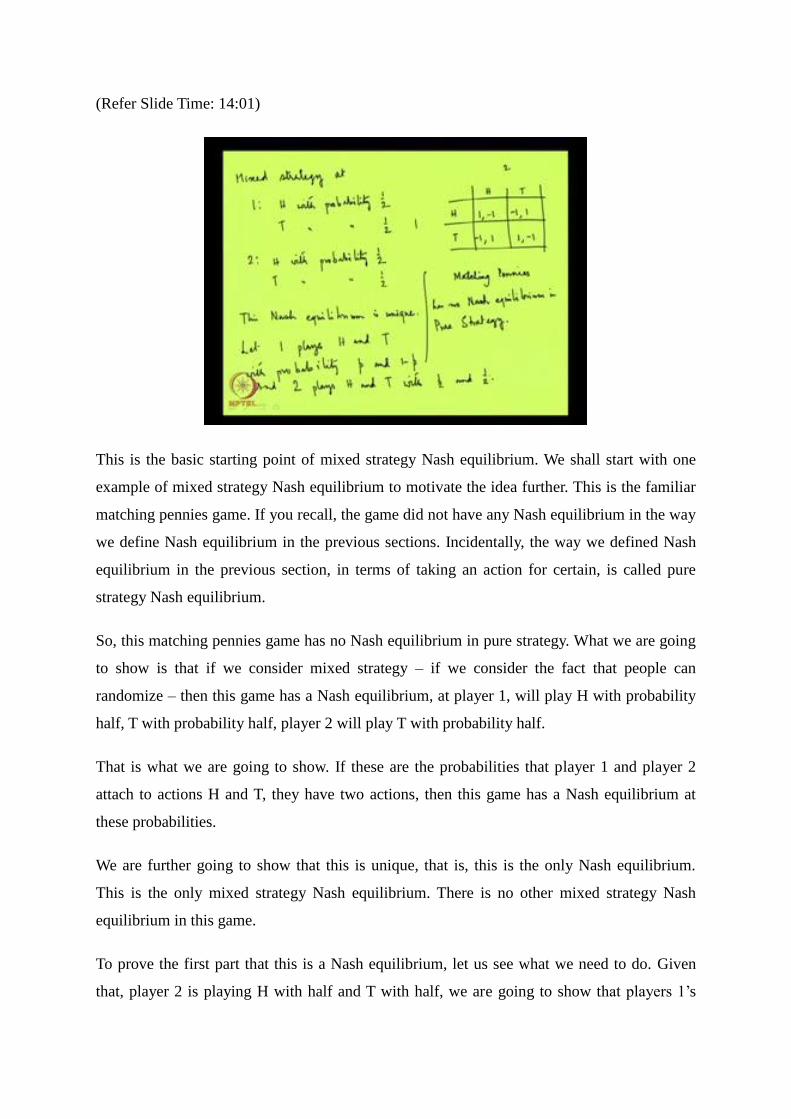
This is the basic starting point of mixed strategy Nash equilibrium. We shall start with one
example of mixed strategy Nash equilibrium to motivate the idea further. This is the familiar
matching pennies game. If you recall, the game did not have any Nash equilibrium in the way
we define Nash equilibrium in the previous sections. Incidentally, the way we defined Nash
equilibrium in the previous section, in terms of taking an action for certain, is called pure
strategy Nash equilibrium.
So, this matching pennies game has no Nash equilibrium in pure strategy. What we are going
to show is that if we consider mixed strategy – if we consider the fact that people can
randomize – then this game has a Nash equilibrium, at player 1, will play H with probability
half, T with probability half, player 2 will play T with probability half.
That is what we are going to show. If these are the probabilities that player 1 and player 2
attach to actions H and T, they have two actions, then this game has a Nash equilibrium at
these probabilities.
We are further going to show that this is unique, that is, this is the only Nash equilibrium.
This is the only mixed strategy Nash equilibrium. There is no other mixed strategy Nash
equilibrium in this game.
To prove the first part that this is a Nash equilibrium, let us see what we need to do. Given
that, player 2 is playing H with half and T with half, we are going to show that players 1’s

playing H with probability half and playing T with probability half, is optimal. Similarly
given player 1 is playing H and T with half and half we are going to show that player 2's
choice of probabilities, that is, half and half is optimal.
(Refer Slide Time: 18:56)
If we can show this then we have shown that this is Nash equilibrium. Instead of half and
half, let us suppose that player 1 plays H and T with probability p and 1 minus p; and 2 plays
these actions with probabilities half and half. Now, if this is the case then what we are
essentially saying is the following – he is playing this actions with probability half and half;
and he is playing with these probabilities.
Now, in this game, there are basically two sorts of outcomes. In the sense that what happens
at the end of the day – either player 1 gets 1 rupee or player 1 loses 1 rupee. Now, if I call that
this event of player 1 getting 1 rupee is that event that player 1 likes, then what is the
probability that player 1 gets 1 rupee?
The probability that 1 gets 1 rupee. This can happen under two circumstances – if the result is
H H that both the players are showing heads to each other; or if the result is T T both the
players are showing tails to each other.
These two events that H H and T T are mutually exclusive – if one happens, the other cannot
happen. So I can write it as H H plus T T. What is the probability that H H has happened? It
means that player 1 has chosen H, player 2 has also chosen H.

Now, these are two probabilities. The probability that player 1 chooses H is p. And the fact
the player 2 has chosen H, which is half…these are independent events. Now, if these are
independent events then the probability that H and H has happened is equal to probability that
player 1 has chosen H, multiplied by the probability that 2 has also chosen H.
This is p multiplied by 2 plus 1 minus p multiplied by half, and this is simply half. So the
probability that player 1 gets 1 rupee is half. What is the probability that player 1 loses 1
rupee? Player 1 loses one rupee under two circumstances – if the result is H T or if the result
is T H. This or this. And again like the logic before, what is the probability that H T is
occurring? It is given by p multiplied by half, and this probability T H is 1 minus p multiplied
by half. So we have got half.
Now, the interesting thing to notice here is that irrespective of p, the probability that player 1
gets 1 rupee or loses 1 rupee remains at half. It is independent of p. So whatever p player 1
fixes, whatever p, which means that probability of showing H, player 1 attaches the
probability that he gets 1 rupee or loses 1 rupee, that remains constant at half. Which means
that any p is optimal.
Optimal, in the sense, that player 1 always likes to get 1 rupee, so he would always like to
have as much probability attached to this event as possible. But here any p is optimal because
this is independent…. this half is independent of p. And if any p is optimal, then p is equal to
half is also optimal.
Now, this was from the point of view of player 1. The similar logic can be also applied for
player 2. Here, we are going to look at the game from player 2's point of view. To do that, let
us suppose that player 1 attaches half and half probabilities to H and T, and player 2 attaches
q and 1 minus q to H and T.
Now, in this case, probability that player 2 gets 1 rupee…2 get 1 rupee in this circumstance
and this circumstance. And what is the probability of that? Half q plus half 1 minus q, which
is half. Similarly one can show that the probability of p loses 1 rupee is also half. I am not
going to show this last one, but it is easy to show that. It means that given player 1 is playing
H and T with half and half, the player 2's probability of getting 1 rupee or losing 1 rupee
remains fixed at half. It means that player 2 can attach any probability to H and T and any
such probability will be optimal.

(Refer Slide Time: 26:28)
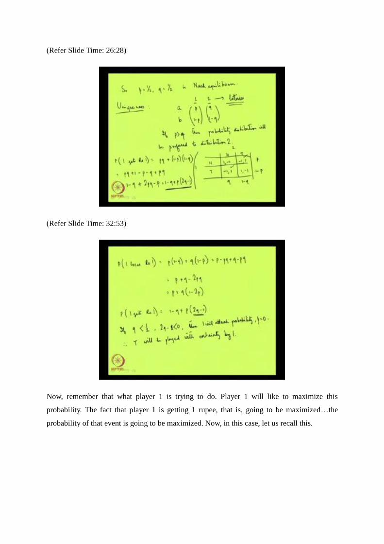
So, any q is optimal. So q is equal to half, is also optimal. What we have derived is the
following – given q is equal to half, p is equal to half is optimal; and given p is equal to half,
q is equal to half is also optimal. And therefore, p is equal to half, q is equal to half, is Nash
equilibrium. That is the proof that in mixed strategy, if we consider mixed strategy, if we
consider that people can randomize, then in matching pennies game, there is a Nash
equilibrium, where p is equal to half, that is, probability of player 1 playing H is equal to half;
and player 2 playing H is also equal to half. This combination of probabilities is a Nash
equilibrium.
Now, the next part is uniqueness – that this is the only Nash equilibrium in this matching
pennies game. To prove that this is the only equilibrium, what we need to assume, which is a
very simple assumption, is that any player will like to maximize the probability of his getting
some higher payoff than not getting some higher payoff. For example, if someone is getting a
and b, under two circumstances, and suppose these are the probabilities, then if p is greater
than q, this is a probability distribution one.
Given that a is preferred to b, the probability distribution where a is getting higher probability
will be preferred by the player. By the way this probability distribution of occurrence of these
events is known as lotteries.
These are lotteries. It is a technical name. A name that we are going to use very often. Now
this is a kind of innocuous assumption but we are going to stick to this assumption. For
proving uniqueness, this assumption is required.
Let us suppose, in general case, that the probabilities attached to these actions by these 2
players, are p, 1 minus p ,q, and 1 minus q. This is the general case.
Like before, what is the probability that player 1 gets 1 rupee? This again occurs if H H
occurs or T T occurs. And the probability of those two occurring are p q plus 1 minus p 1
minus q. And if I simplify this, this is what I get – 1 minus q, 2pq, and minus p.
(Refer Slide Time: 31:34)

(Refer Slide Time: 26:28)
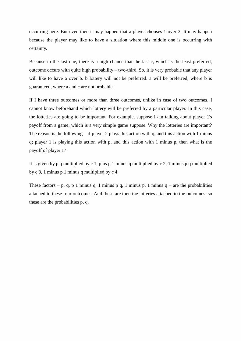
The probability that player 1 gets 1 rupee is 1 minus q plus p multiplied by 2 q minus 1. What
is the probability that 1 loses 1 rupee? So this will be given by if this happens or if this
happens. And the probabilities are p multiplied by 1 minus q, and q multiplied by 1 minus p.
(Refer Slide Time: 32:01)
(Refer Slide Time: 26:28)
(Refer Slide Time: 32:53)
Now, remember that what player 1 is trying to do. Player 1 will like to maximize this
probability. The fact that player 1 is getting 1 rupee, that is, going to be maximized…the
probability of that event is going to be maximized. Now, in this case, let us recall this.

(Refer Slide Time: 26:28)
(Refer Slide Time: 34:46)
If q is… suppose… not equal to half because if q is equal to half, p is also equal to half, and
that is Nash equilibrium. But suppose q is less than half. If q is less than half, then this value
becomes negative. And if this is negative then what should player 1 do? Player 1 should
attach p is equal to 0. Then, player 1 will attach probability p is equal to 0 because this is
negative. These probabilities are sought to be maximized. So p will be said to be equal to 0,
which means T will be played with certainty by player 1.

Now remember, if T is being played with certainty with by player 1, what should player 2 do?
Then player 2 will play H with certainty. In that case, q is becoming equal to 1. So we started
with q less than half, we have seen that if q is less than half then p is equal to 0 and if p is
equal to 0 then q becomes equal to 1. It no longer remains less than half.
So we do not have any Nash equilibrium, if q is less than half… so, no Nash equilibrium.
Similarly, if we take q is greater than half, then what will happen is that this is positive, and p
becomes equal to 1. And if p is equal to 1, then what happens?
(Refer Slide Time: 26:28)
Player 1 is playing this with certainty. In that case, player 2 will play T with certainty. It
means that q is going to be equal to 0. So once again, we have the familiar thing that if we
start with q greater than half, the optimal response from player 1 is that setting p is equal to 1,
and if p is equal to 1, then q becomes equal to 0.

(Refer Slide Time: 36:16)
(Refer Slide Time: 36:35)
We again… we do not have any Nash equilibrium here. It means that if we take any q, which
is not equal to half, we do not have any Nash equilibrium. Similarly we can show, that player
2's probability of gaining…one can show that there is no Nash equilibrium, if p is not equal
to half.
What we have shown is that… no Nash equilibrium…the only Nash equilibrium there is in
this game is where p is equal to half and q is equal to half. The fact that this is a Nash

equilibrium as we have just shown before. And now, we show that this is a unique Nash
equilibrium – there is no other Nash equilibrium. So that is that.
Now to recapitulate what we have done. Let us recapitulate and go to the next step. Here, we
are considering the fact that players have different actions and they randomize. They do not
play any action with certainty. And if they do not play actions with certainty, then the
probability that is any action profile is going to be played remains uncertain – it may have a
probability less than one and greater than 0.
For example, let us take the following game – so this is a1, a2, b1, b2. Let us suppose, player 2
is playing this action with certainty. So this is going to be played.
Now, had player 1 played a1 with certainty, we know that the outcome would have been, let
us suppose, a1 b1, and the payoff from this is c1. Now the deviation that player 1 can take is he
can go to a2, and then the outcome becomes a2b1, and the payoff becomes c2.
So, player 1, when he is deviating, needs to consider between c1 and c2. This is not a very
difficult task. This was the case of pure strategy. But when we have these two actions by
player 1 – he has only two actions to choose from – and he is considering deviation from this
action a1, then there can be infinite number of deviations because he can randomize.
These are the two actions. Suppose the probabilities are p1. Let us not write p1, let us call this,
1/10, and this is 9/10, or can be half half. So, there are infinite numbers of such possibilities.
If there are infinite numbers of such possibilities, then player 1 has to compare all these
possibilities – the payoff from all this possibilities – with what he is getting at present, which
is c1.
So, the task becomes little difficult. It becomes even more difficult, if there are suppose three
actions. Suppose I have another… three – another action. Now, previously there were just
two actions to choose from. Now I have another action a3. Previously, it was easy to see if I
do not have a3 ….suppose, if c1 is more than c2, then which one will be more preferred. All
these lotteries – suppose this is p1, this p2, etc. That lottery will be most preferred by player 1,
where the value attached to this a1 is the highest. Because from a1, he is getting c1, which is
higher than c2, which he is getting from a2.

So, whenever the probability of occurring of a1 b1 is there, that probability will be sought to
be maximized by player 1, if there are only two actions a1 and a2. But if there are three action,
the story becomes more complicated. Then, it is not that simple rule of thumb that you attach
higher probability, where the payoff is higher. The story becomes even more complicated, if
player 2 is not playing this with certainty, but, suppose, he is also randomizing.
In that case also, this maximization of probability attached to a1 is not going to be optimal. It
is because I do not know whether that action is going to be played with certainty … that
outcome will happen with certainty. So if I have more than one two actions, or more than two
outcomes, then the lottery or the preference of lotteries becomes a little difficult to figure out.
(Refer Slide Time: 43:51)
It is like this. This is the preference of a player – a is preferred over b. And the model that we
had so far -- if there are two outcomes, then if p is greater than q, and these are two lotteries –
lottery 1 is preferred over lottery 2. Suppose, I have three outcomes and I know the
preference ordering of the outcomes. Suppose I have three outcomes – a, b, c. To have a
concrete idea, I am comparing between two lotteries. This is one lottery and this is another
lottery.
Now can we say for certain, whether 1 will be preferred to 2, or 2 will be preferred to 1? We
cannot. If we do not have any further information regarding player’s preferences. Remember,
here the previous rule of thumb was that if you prefer a, you prefer that lottery where a’s
probability was higher. Here, a’s probability is one-third, which is greater than 0. 0 is
occurring here. But even then it may happen that a player chooses 1 over 2. It may happen
because the player may like to have a situation where this middle one is occurring with
certainty.
Because in the last one, there is a high chance that the last c, which is the least preferred,
outcome occurs with quite high probability – two-third. So, it is very probable that any player
will like to have a over b. b lottery will not be preferred. a will be preferred, where b is
guaranteed, where a and c are not probable.
If I have three outcomes or more than three outcomes, unlike in case of two outcomes, I
cannot know beforehand which lottery will be preferred by a particular player. In this case,
the lotteries are going to be important. For example, suppose I am talking about player 1's
payoff from a game, which is a very simple game suppose. Why the lotteries are important?
The reason is the following – if player 2 plays this action with q, and this action with 1 minus
q; player 1 is playing this action with p, and this action with 1 minus p, then what is the
payoff of player 1?
It is given by p q multiplied by c 1, plus p 1 minus q multiplied by c 2, 1 minus p q multiplied
by c 3, 1 minus p 1 minus q multiplied by c 4.
These factors – p, q, p 1 minus q, 1 minus p q, 1 minus p, 1 minus q – are the probabilities
attached to these four outcomes. And these are then the lotteries attached to the outcomes. so
these are the probabilities p, q.

(Refer Slide Time: 49:33)
They are similar to this p’s here or these p’s here. So, if I have more than two outcomes, then
how does one figure out which lottery one prefers over other lotteries. For this, one
assumption that we are going to take is the preference of the players are von Neumann
Morgenstern, which means that there is a particular kind of preference, which is called von
Neumann Morgenstern preference. The players' preference obey that property – the property
of von Neumann Morgenstern preference. And what does it mean? It means that if a, b, c are
the outcomes and p1, p2, p3 are the probabilities attached to them, then utility or the payoff
from a b c with the probabilities attached p1, p2, p3 is the expected value of the payoff
functions from the certain events.
So this is going to be p1. This and this small u's – these are the payoff functions defined over
deterministic outcomes. These are also called Bernoulli functions: Bernoulli payoff function,
or Bernoulli utility function.
If the preference of the player satisfy von Neumann Morgenstern preference, then it is
possible to rank the different lotteries that the people face. So, if people have… a particular
player, facing two lotteries, suppose one is p1, p2, p3 and another lottery is there where the
probabilities are different – q1, q2, q3 . Then, I apply this formula over this lottery also. And I
get this. Then it is easy to compare. Because this is a number and this is again a number. If
this number is higher than this number, then this lottery is preferred to this lottery and vice
versa. If this number is higher than this number, then this lottery is preferred to this lottery.
And if these two numbers are equal, then the player is indifferent between these two lotteries.
So, this von Neumann Morgenstern preference pattern gives us a clue how to compare the
preference of players over lotteries. Now, it is by no means a sacrosanct kind of assumption
that people’s preferences are going to satisfy von Neumann Morgenstern preference. It may
very well happen that they do not satisfy von Neumann Morgenstern assumption – the
characterization of preference that these are two economists – von Neumann and
Morgenstern. Von Neumann was a computer scientist first, who worked with Morgenstern, an
American economist, and they proposed this kind of preference pattern to deal with cases of
uncertainty.
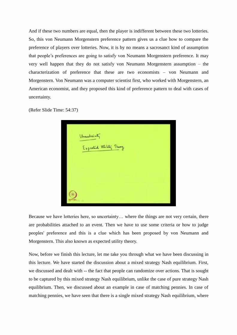
(Refer Slide Time: 54:37)
Because we have lotteries here, so uncertainty… where the things are not very certain, there
are probabilities attached to an event. Then we have to use some criteria or how to judge
peoples' preference and this is a clue which has been proposed by von Neumann and
Morgenstern. This also known as expected utility theory.
Now, before we finish this lecture, let me take you through what we have been discussing in
this lecture. We have started the discussion about a mixed strategy Nash equilibrium. First,
we discussed and dealt with -- the fact that people can randomize over actions. That is sought
to be captured by this mixed strategy Nash equilibrium, unlike the case of pure strategy Nash
equilibrium. Then, we discussed about an example in case of matching pennies. In case of
matching pennies, we have seen that there is a single mixed strategy Nash equilibrium, where
the probabilities are half and half. And then we started the discussion about how to rank
lotteries, which lottery will be preferred to other lotteries, if we have more than two
outcomes. Talking about that we have introduced the idea of von Neumann Morgenstern
preference; we shall continue from this in the next lecture. Thank you
Questions and Answers
(Refer Slide Time: 56:26)
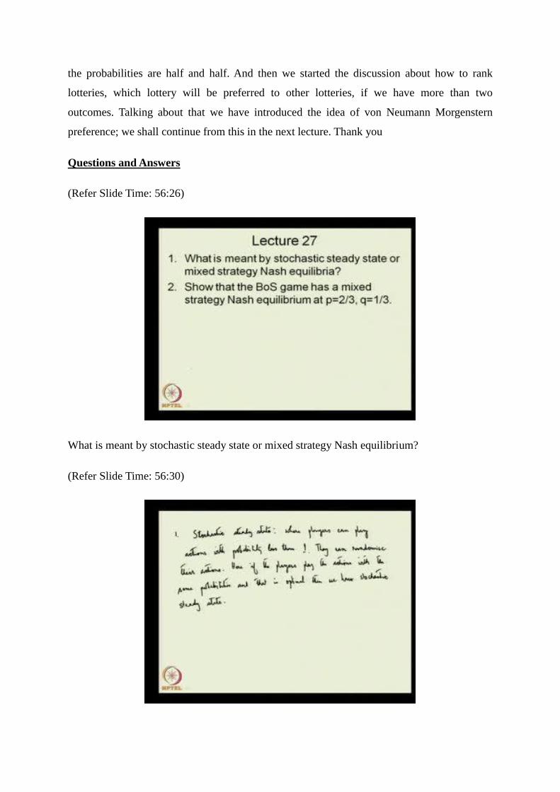
What is meant by stochastic steady state or mixed strategy Nash equilibrium?
(Refer Slide Time: 56:30)
So stochastic steady state -- this is the case where players can play actions with probability
less than 1. They randomize or let us say - they can randomize, they may not randomize -
randomize their actions. Now here, if the players play the actions with the same probabilities
and that is optimal -- same probabilities in each period and that is optimal – then we have
stochastic steady state.
So, here what is not there is that ….it is not required that the players play the same action
every time. What is required is that they play the action with the same probabilities each time.
And that is called as stochastic steady state. Stochastic means related with probability, since
the probabilities are remaining steady, so we are calling it a stochastic steady state. And such
stochastic steady state, if it prevails, will be called a mixed strategy Nash equilibrium.
(Refer Slide Time: 56:26)
(Refer Slide Time: 59:11)
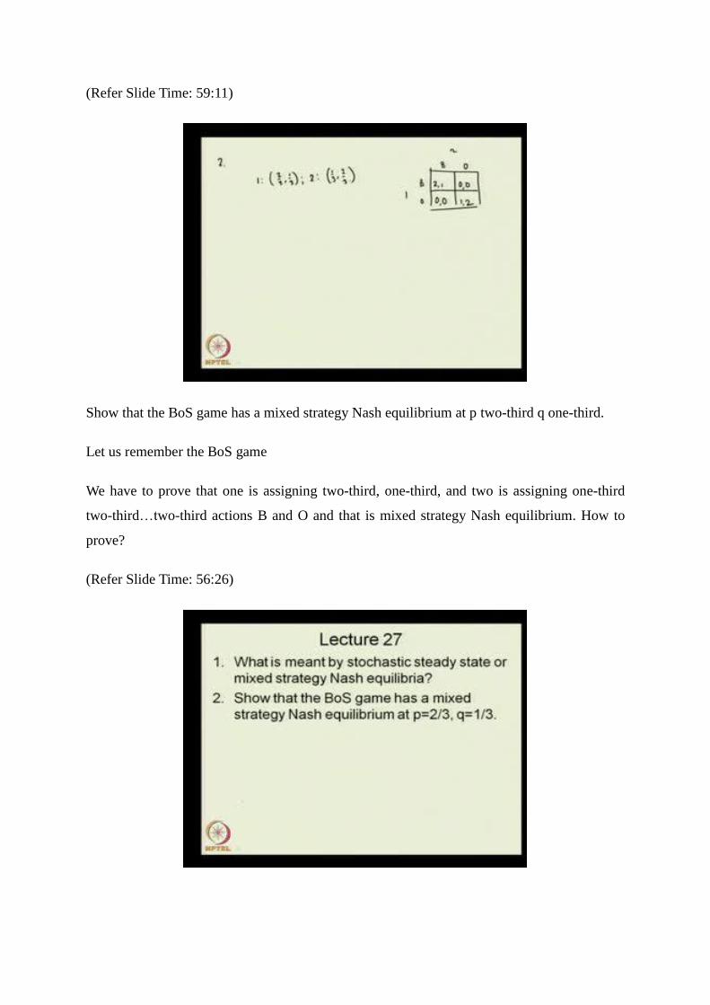
Show that the BoS game has a mixed strategy Nash equilibrium at p two-third q one-third.
Let us remember the BoS game
We have to prove that one is assigning two-third, one-third, and two is assigning one-third
two-third…two-third actions B and O and that is mixed strategy Nash equilibrium. How to
prove?
(Refer Slide Time: 56:26)
(Refer Slide Time: 60:05)
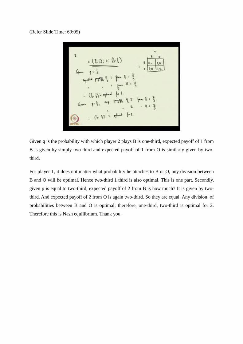
Given q is the probability with which player 2 plays B is one-third, expected payoff of 1 from
B is given by simply two-third and expected payoff of 1 from O is similarly given by two-
third.
For player 1, it does not matter what probability he attaches to B or O, any division between
B and O will be optimal. Hence two-third 1 third is also optimal. This is one part. Secondly,
given p is equal to two-third, expected payoff of 2 from B is how much? It is given by two-
third. And expected payoff of 2 from O is again two-third. So they are equal. Any division of
probabilities between B and O is optimal; therefore, one-third, two-third is optimal for 2.
Therefore this is Nash equilibrium. Thank you.