Proc. Natl. Acad. Sci. USAVol. 90, pp. 4859-4866, June 1993Colloquium Paper

This paper was presented at a colloquium entitled "Physical Cosmology," organized by a committee chaired by DavidN. Schramm, held March 27 and 28, 1992, at the National Academy of Sciences, Irvine, CA.

Galaxy clustering on large scalesG. EFSTATHIOUDepartment of Physics, University of Oxford, OX1 3RH England

ABSTRACT I describe some recent observations of large-scale structure in the galaxy distribution. The best constraintscome from two-dimensional galaxy surveys and studies ofangular correlation functions. Results from galaxy redshiftsurveys are much less precise but are consistent with theangular correlations, provided the distortions in mappingbetween real-space and redshift-space are relatively weak. Thegalaxy two-point correlation function, rich-cluster two-pointcorrelation function, and galaxy-cluster cross-correlationfunction are all well described on large scales (e ; 20h-1 Mpc,where the Hubble constant, Ho = 100h km-s-' Mpc; 1 pc =3.09 x 1016 m) by the power spectrum of an initially scale-invariant, adiabatic, cold-dark-matter Universe with r = Qh

0.2. I discuss how this fits in with the Cosmic BackgroundExplorer (COBE) satellite detection of large-scale anisotropiesin the microwave background radiation and other measures oflarge-scale structure in the Universe.

1. Introduction

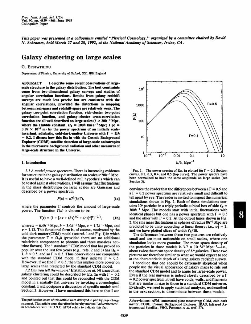
1.1 A modelpower spectrum. There is increasing evidencefor structure in the galaxy distribution on scales -20h-l Mpc.It is useful to have a well-defined null hypothesis which canbe tested against observations. I will assume that fluctuationsin the mass distribution on large scales are Gaussian anddescribed by a power spectrum

P(k) Xc kT2(k/r), [la]

where the parameter r controls the amount of large-scalepower. The function T(x) is chosen to be

T(x) = {1 + [ax + (bx)312 + (cx)2]v}-21v, [lb]

where a = 6.4h-1 Mpc, b = 3.0h-l Mpc, c = 1.7h-1 Mpc, andv = 1.13. This functional form is, of course, motivated by thecold-dark-matter (CDM) model (see ref. 1 and Fig. 1) in whichthe parameter r = Q1oh (provided there are no additionalrelativistic components to photons and three massless neu-trino flavors). The "standard" CDM model that has proved sopopular over the last few years (e.g., refs. 2 and 3) has flo =1, h 0.5, and so r 0.5. Thus observations are compatiblewith the standard CDM model if they indicate r 0.5.However, ifwe find r < 0.5, then this implies more power onlarge scales than predicted by the standard CDM model.

1.2 Can you tell them apart? Efstathiou et al. (4) argued thatgalaxy clustering could be described by Eq. la with r = 0.2and pointed out that this could be reconciled with the CDMmodel in a spatially flat universe by invoking a cosmologicalconstant. I will postpone a discussion of specific models untilSection 3. However, I have mentioned this here so that I can

The publication costs of this article were defrayed in part by page chargepayment. This article must therefore be hereby marked "advertisement"in accordance with 18 U.S.C. §1734 solely to indicate this fact.

FIG. 1. The power spectra of Eq. la plotted for r = 0.1 (bottomcurve), 0.2, 0.3, 0.4, and 0.5 (top curve). The power spectra havebeen normalized to have the same amplitude on large scales (seeSection 3).

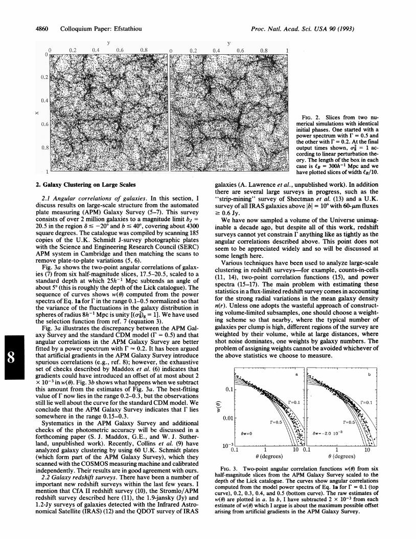
convince the reader that the differences between a F = 0.5 anda F = 0.2 power spectrum are relatively small and difficult totell apart by eye. The reader is invited to inspect the numericalsimulations shown in Fig. 2. Each of these simulations con-tains 106 particles in a triply periodic cubical box of side eB =300h'1 Mpc. The models start with initial fluctuations withidentical phases but one has a power spectrum with F = 0.5and the other with r = 0.2. At the output times shown in Fig.2, the rms mass fluctuations in spheres ofradius 8h-1 Mpc arepredicted to be unity according to linear theory; i.e., of = 1,and we have plotted slices of width eB/10.The differences between these two pictures are relatively

small and are most noticeable on small scales, where onesimulation looks more granular. The mean space density ofthe particles in these models is 3.7 x 10-2h3 Mpc3-i.e.,about twice the mean space density ofL* galaxies. These twopictures are therefore similar to what we would expect to seeat the characteristic depth of a large galaxy redshift survey.

I conclude that one should be extremely skeptical whenpeople use the visual appearance of galaxy maps to rule outthe standard CDM model and to argue for large-scale power.Even if the real universe is indeed closely described by a F= 0.2 power spectrum, it will have voids, walls, and filamentsthat are similar in size to those in a standard CDM universe.Evidently, we need to apply statistical analyses, as describedin the next section, to discriminate between these models.

Abbreviations: APM, automated plate measuring; CDM, cold darkmatter; COBE, Cosmic Background Explorer; IRAS, Infrared As-tronomical Satellite; PHG, Postman et al. (ref. 27).

4859

104

1000

100

10

k/h Mpc-

10

4860 Colloquium Paper: Efstathiou

FIG. 2. Slices from two nu-merical simulations with identicalinitial phases. One started with apower spectrum with F = 0.5 andthe other with F = 0.2. At the finaloutput times shown, o8 = 1 ac-

cording to linear perturbation the-ory. The length of the box in eachcase is eB = 300h-1 Mpc and wehave plotted slices of width tB/10.

2. Galaxy Clustering on Large Scales

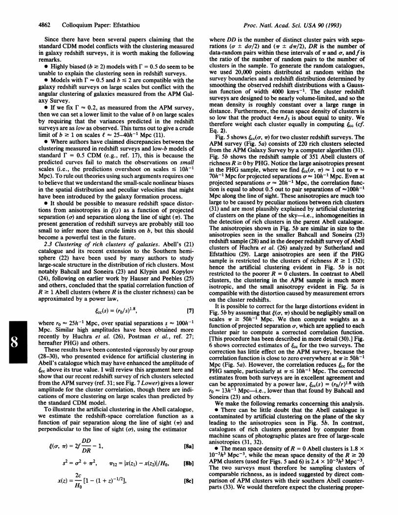
2.1 Angular correlations of galaxies. In this section, Idiscuss results on large-scale structure from the automatedplate measuring (APM) Galaxy Survey (5-7). This surveyconsists of over 2 million galaxies to a magnitude limit bj =20.5 in the region 8 S -20° and b S 400, covering about 4300square degrees. The catalogue was compiled by scanning 185copies of the U.K. Schmidt J-survey photographic plateswith the Science and Engineering Research Council (SERC)APM system in Cambridge and then matching the scans toremove plate-to-plate variations (5, 6).

Fig. 3a shows the two-point angular correlations of galax-ies (7) from six half-magnitude slices, 17.5-20.5, scaled to astandard depth at which 25h-1 Mpc subtends an angle ofabout 50 (this is roughly the depth of the Lick catalogue). Thesequence of curves shows w(6) computed from the powerspectra of Eq. la for F in the range 0.1-0.5 normalized so thatthe variance of the fluctuations in the galaxy distribution inspheres ofradius 8h-1 Mpc is unity [(oj2)g = 1]. We have usedthe selection function from ref. 7 (equation 3).

Fig. 3a illustrates the discrepancy between the APM Gal-axy Survey and the standard CDM model (F = 0.5) and thatangular correlations in the APM Galaxy Survey are betterfitted by a power spectrum with F 0.2. It has been argued

that artificial gradients in the APM Galaxy Survey introducespurious correlations (e.g., ref. 8); however, the exhaustiveset of checks described by Maddox et al. (6) indicates thatgradients could have introduced an offset of at most about 2X 10-3 in w(O). Fig. 3b shows what happens when we subtractthis amount from the estimates of Fig. 3a. The best-fittingvalue of r now lies in the range 0.2-0.3, but the observationsstill lie well about the curve for the standard CDM model. Weconclude that the APM Galaxy Survey indicates that liessomewhere in the range 0.15-0.3.

Systematics in the APM Galaxy Survey and additionalchecks of the photometric accuracy will be discussed in aforthcoming paper (S. J. Maddox, G.E., and W. J. Suther-land, unpublished work). Recently, Collins et al. (9) haveanalyzed galaxy clustering by using 60 U.K. Schmidt plates(which form part of the APM Galaxy Survey), which theyscanned with the COSMOS measuring machine and calibratedindependently. Their results are in good agreement with ours.

2.2 Galaxy redshift surveys. There have been a number ofimportant new redshift surveys within the last few years. Imention that CfA II redshift survey (10), the Stromlo/APMredshift survey described here (11), the 1.9-jansky (Jy) and1.2-Jy surveys of galaxies detected with the Infrared Astro-nomical Satellite (IRAS) (12) and the QDOT survey of IRAS

galaxies (A. Lawrence et al., unpublished work). In additionthere are several large surveys in progress, such as the"strip-mining" survey of Shectman et al. (13) and a U.K.survey of all IRAS galaxies above Ibl = 100 with 60-gm fluxes.0.6 Jy.We have now sampled a volume of the Universe unimag-

inable a decade ago, but despite all of this work, redshiftsurveys cannot yet constrain F anything like as tightly as theangular correlations described above. This point does notseem to be appreciated widely and so will be discussed atsome length here.Various techniques have been used to analyze large-scale

clustering in redshift surveys-for example, counts-in-cells(11, 14), two-point correlation functions (15), and powerspectra (15-17). The main problem with estimating thesestatistics in a flux-limited redshift survey comes in accountingfor the strong radial variations in the mean galaxy densityn(r). Unless one adopts the wasteful approach of construct-ing volume-limited subsamples, one should choose a weight-ing scheme so that nearby, where the typical number ofgalaxies per clump is high, different regions of the survey areweighted by their volume, while at large distances, whereshot noise dominates, one weights by galaxy numbers. Theproblem of assigning weights cannot be avoided whichever ofthe above statistics we choose to measure.

1 10 0.1 10 (degrees) 0 (degrees)

FIG. 3. Two-point angular correlation functions w(O) from sixhalf-magnitude slices from the APM Galaxy Survey scaled to thedepth of the Lick catalogue. The curves show angular correlationscomputed from the model power spectra of Eq. la for F = 0.1 (topcurve), 0.2, 0.3, 0.4, and 0.5 (bottom curve). The raw estimates ofw(O) are plotted in a. In b, I have subtracted 2 x 10-3 from eachestimate of w(O) which I argue is about the maximum possible offsetarising from artificial gradients in the APM Galaxy Survey.

3, y

0.2

0.4

0.6

0.8

Proc. Natl. Acad. Sci. USA 90 (1993)

Proc. Natl. Acad. Sci. USA 90 (1993) 4861

For example, the variance in the sample estimate of thespatial correlation function k(s) in the region f : 1 isminimized approximately ifwe assign to each galaxy of a pairwith redshift-space separation s a weight

wi 1/[1 + 41irn(rj)J3(s)], [2]

where J3(s) = flo (x)x2 dx (11) and ri is the radial distance ofthe ith galaxy. Evidently, we require a prior model for c(s) toapply Eq. 2. Similar remarks apply to estimates of the powerspectra, where the optimal weights for the galaxies are afunction of the wavenumber.

Estimating two-point correlations in redshift surveys iscomplex, and it is even more difficult to estimate reliable errorbars since these depend on unknown higher-order statistics ofthe galaxy distribution. A more pragmatic approach, adoptedby several groups, is to fix on a particular weighting schemeor statistic and then to simulate the observations as closely aspossible within a particular theoretical framework by usingN-body simulations. If the simulations fail to reproduce theobservations, then it is reasonable to conclude that the modeldiffers from the data. The problem here is that the theoreticalpredictions may be sensitive to poorly understood details ofthe model. For example, in a biased CDM model we have toknow how to associate galaxies with mass fluctuations, and theway that this is done can affect the statistical properties of theresulting point process.Here I discuss results from applying counts-in-cells to the

QDOT and Stromlo/APM surveys. These redshift surveysare based on random samples from their parent catalogues.The QDOT survey consists of 2163 galaxies with 60-,gmfluxes . 0.6 Jy selected at a rate of 1 in 6 from the IRAS PointSource Catalog. The Stromlo/APM redshift survey consistsof 1787 galaxies selected at random at a rate of 1 in 20 fromthe APM Galaxy Survey to a magnitude limit of bj = 17.15(see Fig. 7 Upper). Further results on the clustering in thesetwo surveys can be found in refs. 11, 14, and 18.To apply the counts-in-cells analysis, we divide up space

into concentric shells of radial width e centered on theobserver. These are subdivided further into roughly cubicalcells of volume V = e3. We define the statistics

_ 1N= - Ni,

M i

1

(M-1)i

likelihood function, and we estimate approximate 95% errorsfrom the values of o-2 where the likelihood function falls bya factor of 6.82 from its maximum value.The counts-in-cells variances for the two surveys are

plotted in Fig. 4. Notice that the variances for IRAS andoptical galaxies are surprisingly similar on scales - 20h-1Mpc, whereas on scales : lOh-1 Mpc, IRAS galaxies aremore weakly clustered than optical galaxies (e.g., ref. 19).The QDOT point at ( = 40h-1 Mpc looks like an upwardfluctuation, and from a comparison of the QDOT survey andthe larger 1.2-Jy survey, we now know this to be true.The two lines in the figure show computations of a-2(e) for

the power spectra of Eq. 1. As with the computation of w(6),we have normalized the power spectra so that (oj)g = 1.However, to compare with the observations of o-2 in Fig. 4 weneed to take into account the distortion caused by mappingbetween real space and redshift space. In linear theory, thisgives

2(e):/ 2 f0.6 1 fl_2\2() t1 + -- + _ _~Cr [6]

(20), where the subscript s denotes an estimate in redshiftspace and r denotes an estimate in real space, and b is thebiasing factor on scale e(defined by o2 = b2or2, where o72is the mean square fluctuation in the mass distribution). Asimilar equation relates correlations in redshift space, 4(s),to correlations in real space, 4(s). In Fig. 4, we have assumedas = 1.4ao, as appropriate for b = 2flQ6. The dotted line lieslow compared to the observed estimates Oust clipping the95% error bars), and so the standard CDM model with b - 2provides a poor description of the observations. However,the differences between the theoretical models and the ob-servations are similar to the uncertainties in correction for thedistortion between real space and redshift space. Since theerrors on the observed variances in Fig. 4 are so large, theobservations lack the precision to distinguish between theshapes of curves with different F. Thus a curve with F = 0.5can provide an acceptable fit if b is lowered below 2, and sincelow values of b for this type of model are implied by theCosmic Background Explorer (COBE) observations (seeSection 3), it may be that the standard CDM model iscompatible with the redshift survey results after all.

where the sums extend over the M cells in each radial shelland Ni is the galaxy count in the ith cell. The expectationvalues of these statistics are

(N) = nV, (S) = n2V2co2

l

O r (rl2) dV,dV2,

1

[4a]

[4b] I-Icgb

0.1

and so we can estimate o2 in each radial shell. The varianceson these estimates depend on the detailed statistical proper-ties of the galaxy distribution, but if we assume that the cellsare independent, and that underlying fluctuations are Gauss-ian, we can show that

Var(S) =2n2V2(1 + v.2) + 4n3V3Cr2 + 2n4V4cr4

M

where n is the mean density in each radial shell. The estimatesof oa2 from different radial shells can then be combined byconstructing a likelihood function (equation 7 of ref. 14) on

the assumption that the statistic S is normally distributed withvariance given by Eq. 5 and n N/V. Thus, for each cell size

we estimate a "best fit" value of a'2 which maximizes the

0.01([5] 10 100

I (h-1 Mpc)FIG. 4. The variances in cubical cells of side e determined from

the Stromlo/APM redshift survey (s) and the QDOT survey of IRASgalaxies (o). The error bars show 95% confidence limits computed asdescribed in the text. The two curves show a'2(i) computed for thepower spectra of Eq. la. In each case we have assumed that c2measured in redshift space is 1.4 times cr2 in real space.

Colloquium Paper: Efstathiou

4862 Colloquium Paper: Efstathiou

Since there have been several papers claiming that thestandard CDM model conflicts with the clustering measuredin galaxy redshift surveys, it is worth making the followingremarks.* Highly biased (b . 2) models with F = 0.5 do seem to be

unable to explain the clustering seen in redshift surveys.* Models with F 0.5 and b S 2 are compatible with the

galaxy redshift surveys on large scales but conflict with theangular clustering of galaxies measured from the APM Gal-axy Survey.

* If we fix F 0.2, as measured from the APM survey,then we can set a lower limit to the value of b on large scalesby requiring that the variances predicted in the redshiftsurveys are as low as observed. This turns out to give a crudelimit of b - 1 on scales e 25-40h-1 Mpc (11).* Where authors have claimed discrepancies between the

clustering measured in redshift surveys and low-b models ofstandard F = 0.5 CDM (e.g., ref. 17), this is because thepredicted curves fail to match the observations on smallscales (i.e., the predictions overshoot on scales S lOh-Mpc). To rule out theories using such arguments requires oneto believe that we understand the small-scale nonlinear biasesin the spatial distribution and peculiar velocities that mighthave been introduced by the galaxy formation process.* It should be possible to measure redshift space distor-

tions from anisotropies in e(s) as a function of projectedseparation (a) and separation along the line of sight (ir). Thepresent generation of redshift surveys are probably still toosmall to infer more than crude limits on b, but this shouldbecome a powerful test in the future.

2.3 Clustering of rich clusters of galaxies. Abell's (21)catalogue and its recent extension to the Southern hemi-sphere (22) have been used by many authors to studylarge-scale structure in the distribution of rich clusters. Mostnotably Bahcall and Soneira (23) and Klypin and Kopylov(24), following on earlier work by Hauser and Peebles (25)and others, concluded that the spatial correlation function ofR - 1 Abell clusters (where R is the cluster richness) can beapproximated by a power law,

ec.(S) = (ro/s)"8, [7]

where ro 25h-1 Mpc, over spatial separations s lOOh-1Mpc. Similar high amplitudes have been obtained morerecently by Huchra et al. (26), Postman et al., ref. 27;hereafter PHG) and others.These results have been contested vigorously by our group

(28-30), who presented evidence for artificial clustering inAbell's catalogue which may have enhanced the amplitude of&,_ above its true value. I will review this argument here andshow that our recent redshift survey of rich clusters selectedfrom the APM survey (ref. 31; see Fig. 7 Lower) gives a loweramplitude for the cluster correlation, though there are indi-cations of more clustering on large scales than predicted bythe standard CDM model.To illustrate the artificial clustering in the Abell catalogue,

we estimate the redshift-space correlation function as afunction of pair separation along the line of sight (ir) andperpendicular to the line of sight (a), using the estimator

DD{(a, ir) = 2f D--1, [8a]DR

-2 0.o2 + 1r2, '712 = 1X(Z1) - X(Z2)I/HO, [Sb]2c

12x(z) =- [1 - (1 + ZY112], [Sc]Ho

where DD is the number of distinct cluster pairs with sepa-rations (oa ± do-/2) and (ir ± d'r/2), DR is the number ofdata-random pairs within these intervals of ir and a, andfisthe ratio of the number of random pairs to the number ofclusters in the sample. To generate the random catalogues,we used 20,000 points distributed at random within thesurvey boundaries and a redshift distribution determined bysmoothing the observed redshift distributions with a Gauss-ian function of width 4000 kms-1. The cluster redshiftsurveys are designed to be nearly volume-limited, and so themean density is roughly constant over a large range indistance. Furthermore, the mean space density of clusters isso low that the product 4'rnJ3 is about equal to unity. Wetherefore weight each cluster equally in computing &, (cf.Eq. 2).

Fig. 5 shows fcr(o, ir) for two cluster redshift surveys. TheAPM survey (Fig. Sa) consists of 220 rich clusters selectedfrom the APM Galaxy Survey by a computer algorithm (31).Fig. Sb shows the redshift sample of 351 Abell clusters ofrichness R 2 0 by PHG. Notice the large anisotropies presentin the PHG sample, where we find &Ja-, ir) 1 out to v70h-1 Mpc for projected separations o -l 10/ Mpc. Even atprojected separations cr 20h-1 Mpc, the correlation func-tion is equal to about 0.5 out to pair separations of 100h-1Mpc along the line of sight. These anisotropies are much toolarge to be caused by peculiar motions between rich clusters(31) and are most plausibly explained by artificial clusteringof clusters on the plane of the sky-i.e., inhomogeneities inthe detection of rich clusters in the parent Abeli catalogue.The anisotropies shown in Fig. Sb are similar in size to theanisotropies seen in the smaller Bahcall and Soneira (23)redshift sample (28) and in the deeper redshift survey ofAbellclusters of Huchra et al. (26) analyzed by Sutherland andEfstathiou (29). Large anisotropies are seen if the PHGsample is restricted to the clusters of richness R 2 1 (32);hence the artificial clustering evident in Fig. Sb is notrestricted to the poorer R = 0 clusters. In contrast to Abellclusters, the clustering in the APM sample is much moreisotropic, and the small anisotropy evident in Fig. Sa iscompatible with the distortion caused by measurement errorson the cluster redshifts.

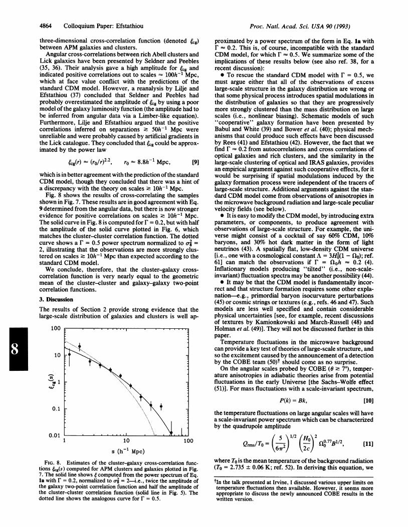
It is possible to correct for the large distortions evident inFig. Sb by assuming that e(or, ir) should be negligibly small onscales ir - SOh-1 Mpc. We then compute weights as afunction of projected separation a-, which are applied to eachcluster pair to compute a corrected correlation function.[This procedure has been described in more detail (30).] Fig.6 shows corrected estimates of &cc for the two surveys. Thecorrection has little effect on the APM survey, because thecorrelation function is close to zero everywhere at ir 2 50h-1Mpc (Fig. Sa). However, the correlation reduces &,_ for thePHG sample, particularly at irS lOh-1 Mpc. The correctedestimates from both surveys are in excellent agreement andcan be approximated by a power law, 4c_(s) = (ro/r)1 8 withro 13h-1 Mpc-i.e., lower than that found by Bahcall andSoneira (23) and others.We make the following remarks concerning this analysis.* There can be little doubt that the Abeli catalogue is

contaminated by artificial clustering on the plane of the skyleading to the anisotropies seen in Fig. 5b. In contrast,catalogues of rich clusters generated by computer frommachine scans of photographic plates are free of large-scaleanisotropies (31, 32).* The mean space density ofR = 0 Abell clusters is 1.8 x

10-5h3 Mpc-3, while the mean space density of the R - 20APM clusters (used for Figs. S and 6) is 2.4 x 10-5h3 Mpc-3.The two surveys must therefore be sampling clusters ofcomparable richness, as is indeed suggested by direct com-parison of APM clusters with their southern Abell counter-parts (33). We would therefore expect the clustering proper-

Proc. Natl. Acad Sci. USA 90 (1993)

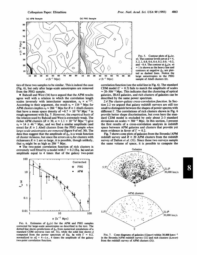
Proc. Natl. Acad. Sci. USA 90 (1993) 4863

(a) APM Sample (b) PHG Sample

90

80

70

i.z 60

_ 50

t1 40

30

20

10

40 50 60 70 80 90 10 20 30 40 50 60

a- (h'I Mpc) a- (h-1 Mpc)

ties of these two samples to be similar. This is indeed the case(Fig. 6), but only after large-scale anisotropies are removedfrom the PHG sample.* Bahcall and West (34) have argued that the APM results

agree well with a relation in which the correlation lengthscales inversely with intercluster separation, ro o n-1/3.According to their argument, the result ro = 13h-1 Mpc forAPM clusters implies ro 20h-1 Mpc forR 2 1 Abeil clustersthat have a mean space density of =0.7 x 10-5h3 Mpc-3 inrough agreement with Eq. 7. However, the empirical basis ofthe relation used by Bahcall and West is extremely weak. Thericher APM clusters (R 2 30, n 1.1 x 10-5h3 Mpc-3) givero 14 + 4h-1 Mpc, and we find a similar amplitude (anderror) for R 2 1 Abell clusters from the PHG sample whenlarge-scale anisotropies are removed (figure 9 of ref. 30). Thedata thus suggest that the amplitude of fcc is a weak functionof cluster richness, but since the errors on ro for clusters withrichnesses R - 1 are so large, it is possible, though unlikely,that ro might be as high as 20h-1 Mpc.* The two-point correlation function of rich clusters is

extremely well fitted by a model with F = 0.2 (Eq. la) and anamplitude equal to 4 times that of the galaxy two-point

100

10

0W

8 1

0.1

0.011 10

FIG. 5. Contour plots of 4c(r,ir). The contour levels are at f = 4,3, 2, 1, 0.8, 0.6, 0.4, 0.2, 0.0, -0.2,and -0.4. The contour at cc(, ii)= 1 is shown as the heavy line andcontours at negative e,, are plot-ted as dashed lines. Notice thelarge anisotropies in the PHGsample of Abell clusters (b).

correlation function (see the solid line in Fig. 6). The standardCDM model (F = 0.5) fails to match the amplitude of scales

20-30h-1 Mpc. This indicates that the clustering of opticalgalaxies, IRAS galaxies, and rich clusters of galaxies can bedescribed by the same power spectrum.

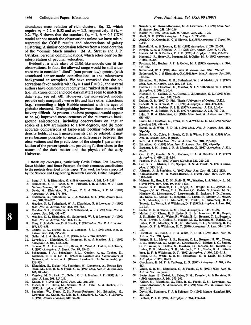
2.4 The cluster-galaxy cross-correlation function. In Sec-tion 2.2 we argued that galaxy redshift surveys are still toosmall to distinguish between the shapes ofpower spectra withdifferent r. The correlations of rich clusters shown in Fig. 6provide better shape discrimination, but even here the stan-dard CDM model is excluded by only about 2-3 standarddeviations on scales 30h-1 Mpc. In this section, I presentthe first results of a cross-correlation analysis in redshiftspace between APM galaxies and clusters that provide yetmore evidence in favor of F 0.2.

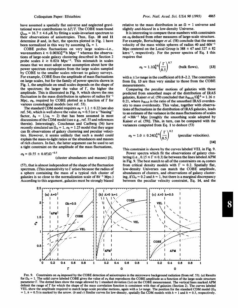
Fig. 7 shows cone plots of galaxies from the Stromlo/APMredshift survey and R - 20 APM clusters from the redshiftsurvey of Dalton et al. (31). Since these two surveys samplethe same volume of space, it is possible to compute the

Galaxies

5r 4 5, 3;000,000 km/s

100

s (h-1 Mpc)FIG. 6. Estimates of &,,(s) for the APM and PHG samples

corrected for large-scale anisotropies as described in the text. Thedotted line shows predictions of ec, from numerical simulations of astandard CDM universe (see ref. 31), while the solid line shows fcomputed from the power spectrum of Eq. la with r = 0.2,normalized to a- = 4-i.e., 4 times the amplitude of the galaxytwo-point correlation function.

0

FIG. 7. Cone diagrams of galaxies (Upper) within 30,000 km's-1in the Stromlo/APM redshift survey (11) and rich clusters (Lower)from the redshift survey of APM clusters (31).

Colloquium Paper: Efstathiou

4864 Colloquium Paper: Efstathiou

three-dimensional cross-correlation function (denoted &g)between APM galaxies and clusters.

Angular cross-correlations between rich Abell clusters andLick galaxies have been presented by Seldner and Peebles(35, 36). Their analysis gave a high amplitude for fcg andindicated positive correlations out to scales lOOh-1 Mpc,which at face value conflict with the predictions of thestandard CDM model. However, a reanalysis by Lilje andEfstathiou (37) concluded that Seldner and Peebles hadprobably overestimated the amplitude of fcg by using a poormodel ofthe galaxy luminosity function (the amplitude had tobe inferred from angular data via a Limber-like equation).Furthermore, Lilje and Efstathiou argued that the positivecorrelations inferred on separations z 50h-1 Mpc wereunreliable and were probably caused by artificial gradients inthe Lick catalogue. They concluded that &g could be approx-imated by the power law

4cg(r) (ro/r)22, ro 8.8h-1 Mpc, [9]

which is in better agreement with the prediction ofthe standardCDM model, though they concluded that there was a hint ofa discrepancy with the theory on scales - lOh-1 Mpc.

Fig. 8 shows the results of cross-correlating the samplesshown in Fig. 7. These results are in good agreement with Eq.9 determined from the angular data, but there is now strongerevidence for positive correlations on scales z lOh-1 Mpc.The solid curve in Fig. 8 is computed for F = 0.2, but with halfthe amplitude of the solid curve plotted in Fig. 6, whichmatches the cluster-cluster correlation function. The dottedcurve shows a = 0.5 power spectrum normalized to =

2, illustrating that the observations are more strongly clus-tered on scales lOh-1 Mpc than expected according to thestandard CDM model.We conclude, therefore, that the cluster-galaxy cross-

correlation function is very nearly equal to the geometricmean of the cluster-cluster and galaxy-galaxy two-pointcorrelation functions.

3. Discussion

The results of Section 2 proyide strong evidence that thelarge-scale distribution of galaxies and clusters is well ap-

100

10

C,_S

0.1

0.011 10

s (h-1 Mpc)

proximated by a power spectrum of the form in Eq. la with0.2. This is, of course, incompatible with the standard

CDM model, for which r 0.5. We summarize some of the

implications of these results below (see also ref. 38, for arecent discussion):* To rescue the standard CDM model with r = 0.5, we

must argue either that all of the observations of excesslarge-scale structure in the galaxy distribution are wrong orthat some physical process introduces spatial modulations inthe distribution of galaxies so that they are progressivelymore strongly clustered than the mass distribution on largescales (i.e., nonlinear biasing). Schematic models of such"cooperative" galaxy formation have been presented byBabul and White (39) and Bower et al. (40); physical mech-anisms that could produce such effects have been discussedby Rees (41) and Efstathiou (42). However, the fact that wefind 0.2 from autocorrelations and cross correlations of

optical galaxies and rich clusters, and the similarity in thelarge-scale clustering of optical and IRAS galaxies, providesan empirical argument against such cooperative effects, for itwould be surprising if spatial modulations induced by thegalaxy formation process were independent of the tracers oflarge-scale structure. Additional arguments against the stan-dard CDM model come from observations of anisotropies inthe microwave background radiation and large-scale peculiarvelocity fields (see below).

* It is easy to modify the CDM model, by introducing extraparameters, or components, to produce agreement withobservations of large-scale structure. For example, the uni-verse might consist of a cocktail of say 60% CDM, lo0baryons, and 30%o hot dark matter in the form of lightneutrinos (43). A spatially flat, low-density CDM universe[i.e., one with a cosmological constant A = 3Ho(1 - DO); ref.61] can match the observations if r floh 0.2 (4).Inflationary models producing "tilted" (i.e., non-scale-invariant) fluctuation spectra may be another possibility (44).* It may be that the CDM model is fundamentally incor-

rect and that structure formation requires some other expla-nation-e.g., primordial baryon isocurvature perturbations(45) or cosmic strings or textures (e.g., refs. 46 and 47). Suchmodels are less well specified and contain considerablephysical uncertainties [see, for example, recent discussionsof textures by Kamionkowski and March-Russell (48) andHolman et al. (49)]. They will not be discussed further in thispaper.Temperature fluctuations in the microwave background

can provide a key test oftheories of large-scale structure, andso the excitement caused by the announcement of a detectionby the COBE team (50)t should come as no surprise.On the angular scales probed by COBE (6 t 7°), temper-

ature anisotropies in adiabatic theories arise from potentialfluctuations in the early Universe [the Sachs-Wolfe effect(51)]. For mass fluctuations with a scale-invariant spectrum,

P(k) = Bk, [10]

the temperature fluctuations on large angular scales will havea scale-invariant power spectrum which can be characterizedby the quadrupole amplitude

100= ()1/2) (H°) 77/2 [11]

FIG. 8. Estimates of the cluster-galaxy cross-correlation func-tions &cg(s) computed for APM clusters and galaxies plotted in Fig.7. The solid line shows e computed from the power spectrum of Eq.la with r = 0.2, normalized to CJ2 = 2-i.e., twice the amplitude ofthe galaxy two-point correlation function and half the amplitude ofthe cluster-cluster correlation function (solid line in Fig. 5). Thedotted line shows the analogous curve for r = 0.5.

where To is the mean temperature ofthe background radiation(To = 2.735 + 0.06 K; ref. 52). In deriving this equation, we

tIn the talk presented at Irvine, I discussed various upper limits ontemperature fluctuations then available. However, it seems moreappropriate to discuss the newly announced COBE results in thewritten version.

Proc. Natl. Acad. Sci. USA 90 (1993)

Proc. Natl. Acad. Sci. USA 90 (1993) 4865

have assumed a spatially flat universe and neglected gravi-tational wave contributions to AT/T. The COBE team foundQ,m. = 16.7 4.6 uK by fitting a scale-invariant spectrum totheir observations of anisotropies. Thus, Eqs. 10 and 11determine B and, in fact, the spectra plotted in Fig. 1 havebeen normalized in this way by assuming fio = 1.COBE probes fluctuations on very large scales-i.e.,

wavenumbers k s 0.003fl 41h Mpc-1 whereas the observa-tions of large-scale galaxy clustering described in Section 2probe scales k - 0.02h Mpc-1. This mismatch in scalesmeans that we must adopt some assumption about how thepower spectrum extrapolates from the large scales sampledby COBE to the smaller scales relevant to galaxy surveys.For example, COBE fixes the amplitude of mass fluctuationson large scales, but for the family of power spectra shown inFig. 1, the amplitude on small scales depends on the shape ofthe spectrum; the larger the value of F, the higher theamplitude. This is illustrated in Fig. 9, which shows the rmsfluctuation in the mass distribution in spheres of radius 8h-1Mpc, cr8, required by COBE plotted as a function of forvarious cosmological models (see ref. 53).The standard CDM model requires ac8 = 1.1 + 0.22 (see also

ref. 54), which is well above the value or8 0.5 (or a "biasing"

factor, b8 = 1/ao8 2) that has been assumed in most

discussions oftheCDM model (see e.g., ref. 55 and referencestherein). Interestingly, Couchman and Carlberg (56) haverecently simulated an flo = 1, or8 = 1.25 model that they arguecan fit observations of galaxy clustering and peculiar veloci-ties. However, it seems unlikely that such a model couldexplain the mass-to-light ratios or the abundances and massesof rich clusters. In fact, the latter argument can be used to seta tight constraint on the amplitude of the mass fluctuations,

cr8 = (0.55 ± 0.05)4-0.5(cluster abundances and masses) [12]

(57), that is almost independent ofthe shape ofthe fluctuationspectrum. (This insensitivity to F arises because the radius ofa sphere containing the mass of a typical rich cluster ofgalaxies is so close to the normalization scale of 8h-1 Mpc.)According to this argument, galaxies must be strongly biased

relative to the mass distribution in an fQ = 1 universe andslightly anti-biased in a low-density Universe.

It is interesting to compare these numbers with constraintson cr8 deduced from other measures of large-scale structure.For example, Bertschinger et al. (58) conclude that the meanvelocity of the mass within spheres of radius 40 and 60h-1Mpc centered on the Local Group is 388 ± 67 and 327 ± 82km-s-1, respectively. For the power spectra of Eq. 1 thisrequires that

(bulk flows), [13]

with a ±lcrrange in the coefficient of0.8-2.2. The constraintsfrom Eq. 13 are thus very similar to those from the COBEmeasurements.Comparing the peculiar motions of galaxies with those

predicted from smoothed maps of the distribution of IRASgalaxies, Kaiser et aL (59) concluded that bipAS//I86 = 1.16 +0.21, where b1^As is the ratio of the smoothed IRAS overden-sity to mass overdensity. This value, together with observa-tions offluctuations in the distribution ofIRAS galaxies, leadsto an estimate ofthe variance in the mass fluctuations ofscalesof =30h-1 Mpc [roughly the smoothing scale adopted byKaiser et al. (59)]. This, in turn, can be compared with thevariances computed from Eq. 1 to deduce (53)

a-8 1.0 + 0.24i6( 5. (peculiar velocities).

[14]

This constraint is shown by the curves labeled VEL in Fig. 9.Power spectra which fit the observations of galaxy clus-

tering (i.e., 0.15 s s 0.3) lie between the lines labeled APMin Fig. 9. The best match to all of the constraints on cr8 comesfrom critical density models with r 0.2. Spatially flat,

low-density Universes can match the COBE amplitude,abundances of clusters, and observations of galaxy cluster-ing, if II0 0.2 and h 1, but there is a marginal discrepancy

between the peculiar velocity constraint, Eq. 14, and the

0.5

0 0.2 0.4 0.6 0.8 1 0.2 0.4 0.6 0.8 1 0.2 0.4 0.6 0.8 1

r 0 a

FIG. 9. Constraints on a8 imposed by the COBE detection of anisotropies in the microwave background radiation (from ref. 53). (a) Resultsfor flo = 1. The solid curve labeled COBE gives the value of o8 that reproduces the COBE amplitude as a function of the large-scale structureparameter F. The dotted lines show the range allowed by 1 standard deviation (l) on the COBE measurement. The vertical lines marked APMdelimit the range of F for which the shape of the mass correlation function is consistent with that of galaxies (Section 2). The curves labeledVEL show the amplitude required to match large-scale peculiar motions, again with a l, range. The position for the standard CDM model (flo= 1, h = 0.5) is marked by the arrow. (b and c) Similar curves for low-density, spatially flat CDM models with h = 1 and h = 0.5, respectively.

(b) A>0 h=1U I>~ COBE-\\I I.'

1IN- ~VEL

}' APM1I I

F . .. l .L

Colloquium Paper: Efstathiou

laO.6T, 0.7

0-8 =:: 1 - 0 .5

I'll.-Ie I .

-,-

,I

I

. L i . A. I .A I I . . . . I

4866 Colloquium Paper: Efstathiou

abundance-mass relation of rich clusters, Eq. 12, whichrequire cr8 = 2.2 + 0.52 and cr8 1.2, respectively, if fib =

0.2. Fig. 9 shows that the standard fb = 1, h 0.5 CDM

model cannot match the observations unless we have misin-terpreted the COBE results and observations of galaxyclustering. A similar conclusion follows from a considerationof the "cosmic Mach number" (M. A. Strauss and J. P.Ostriker, personal communication), which relies only on theinterpretation of peculiar velocities.

Evidently, a wide class of CDM-like models can fit theobservations. In fact, the allowed range would be still widerwere we to consider "tilted" (non-power-law) spectra (withassociated tensor-mode contributions to the microwavebackground anisotropies). We have remarked that the ob-servations favor models with flb = 1 and F = 0.2, and severalauthors have commented recently that "mixed dark models"(i.e., mixtures of hot and cold dark matter) seem to match thedata (e.g., see ref. 60). However, the non-zero-A modelsprovide only marginally worse fits and have other attractions(e.g., reconciling a high Hubble constant with the ages ofglobular clusters). Distinguishing between these models willbe very difficult. At present, the best prospects would appearto be (a) improved measurements of the microwave back-ground anisotropies, including observations on angularscales of a few arcminutes to a few degrees, and (b) moreaccurate comparisons of large-scale peculiar velocity anddensity fields. If such measurements can be refined, it mayeven become possible to measure differences between theobservations and the predictions of the simple F parameter-ization of the power spectrum, providing further clues to thenature of the dark matter and the physics of the earlyUniverse.

I thank my colleagues, particularly Gavin Dalton, Jon Loveday,Steve Maddox, and Bruce Peterson, for their enormous contributionsto the projects described in this paper. This work has been supportedby the Science and Engineering Research Council, United Kingdom.

1. Bond, J. R. & Efstathiou, G. (1984) Astrophys. J. 285, L45-L48.2. Blumenthal, G. R., Faber, S. M., Primack, J. R. & Rees, M. J. (1984)

Nature (London) 311, 517-525.3. Davis, M., Efstathiou, G., Frenk, C. S. & White, S. D. M. (1985)

Astrophys. J. 292, 371-394.4. Efstathiou, G., Sutherland, W. J. & Maddox, S. J. (1990) Nature (Lon-

don) 348, 705-707.5. Maddox, S. J., Sutherland, W. J., Efstathiou, G. & Loveday, J. (1990)

Mon. Not. R. Astron. Soc. 243, 692-712.6. Maddox, S. J., Efstathiou, G. & Sutherland, W. J. (1990) Mon. Not. R.

Astron. Soc. 246, 433-457.7. Maddox, S. J., Efstathiou, G., Sutherland, W. J. & Loveday, J. (1990)

Mon. Not. R. Astron. Soc. 242, 43-47.8. Fong, R., Hale-Sutton, D. & Shanks, T. (1992) Mon. Not. R. Astron. Soc.

257, 650-658.9. Collins, C. A., Nichol, R. C. & Lumsden, S. L. (1992) Mon. Not. R.

Astron. Soc. 254, 295-300.10. Geller, M. J. & Huchra, J. P. (1990) Science 246, 897-903.11. Loveday, J., Efstathiou, G., Peterson, B. A. & Maddox, S. J. (1992)

Astrophys. J. 400, L43-L46.12. Strauss, M. A., Huchra, J. P., Davis, M., Yahil, A., Fisher, K. & Tonry,

J. (1992) Astrophys. J. Suppl. Ser. 83, 29-63.13. Schectman, S. A., Schechter, P. L., Oemler, A. A., Tucker, D.,

Kirshner, R. P. & Lin, H. (1992) in Clusters and Superclusters ofGalaxies, ed. Fabian, A. C. (Kluwer, Dordrecht, The Netherlands), pp.351-363.

14. Efstathiou, G., Kaiser, N., Saunders, W., Lawrence, A., Rowan-Rob-inson, M., Ellis, R. S. & Frenk, C. S. (1990) Mon. Not. R. Astron. Soc.247, l0p-14p.

15. Vogeley, M. S., Park, C., Geller, M. J. & Huchra, J. P. (1992) Astro-phys. J. Lett. 391, L5-L8.

16. Kaiser, N. (1991) AIP Conf. Proc. 222, 248-260.17. Fisher, K. B., Davis, M., Strauss, M. A., Yahil, A. & Huchra, J. P.

(1993) Astrophys. J. 402, 42-57.18. Saunders, W., Frenk, C. S., Rowan-Robinson, M., Efstathiou, G.,

Lawrence, A., Kaiser, N., Ellis, R. S., Crawford, J., Xia, X.-Y. & Parry,I. (1991) Nature (London) 349, 32-38.

19. Saunders, W., Rowan-Robinson, M. & Lawrence, A. (1992) Mon. Not.R. Astron. Soc. 258, 134-146.

20. Kaiser, N. (1987) Mon. Not. R. Astron. Soc. 227, 1-21.21. Abell, G. 0. (1958) Astrophys. J. Suppl. 3, 211-288.22. Abell, G. O., Corwin, H. C. & Olowin, R. (1989)Astrophys. J. Suppl. 70,

1-138.23. Bahcall, N. A. & Soneira, R. M. (1983) Astrophys. J. 270, 20-38.24. Klypin, A. A. & Kopylov, A. I. (1983) Sov. Astron. Lett. 9, 41-56.25. Hauser, M. G. & Peebles, P. J. E. (1973) Astrophys. J. 185, 757-785.26. Huchra, J. P., Henry, P., Postman, M. & Geller, M. J. (1990) Astrophys.

J. 365, 66-85.27. Postman, M., Huchra, J. P. & Geller, M. J. (1992) Astrophys. J. 384,

404-422.28. Sutherland, W. J. (1988) Mon. Not. R. Astron. Soc. 234, 159-172.29. Sutherland, W. J. & Efstathiou, G. (1991) Mon. Not. R. Astron. Soc. 248,

159-167.30. Efstathiou, G., Dalton, G. B., Sutherland, W. J. & Maddox, S. J. (1992)

Mon. Not. R. Astron. Soc. 257, 125-134.31. Dalton, G. B., Efstathiou, G., Maddox, S. J. & Sutherland, W. J. (1992)

Astrophys. J. 390, L1-L4.32. Nichol, R. C., Collins, C. A., Guzzo, L. & Lumsden, S. L. (1992) Mon.

Not. R. Astron. Soc. 255, 21-24.33. Dalton, G. B. (1992) D. Phil. Thesis (University of Oxford, U.K.).34. Bahcall, N. A. & West, M. J. (1992) Astrophys. J. 392, 419-423.35. Seldner, M. & Peebles, P. J. E. (1977) Astrophys. J. 214, Li-LA.36. Seldner, M. & Peebles, P. J. E. (1977) Astrophys. J. 215, 703-716.37. Lilje, P. B. & Efstathiou, G. (1988) Mon. Not. R. Astron. Soc. 231,

635-655.38. Davis, M., Efstathiou, G., Frenk, C. S. & White, S. D. M. (1992) Nature

(London) 356, 489-494.39. Babul, A. & White, S. D. M. (1991) Mon. Not. R. Astron. Soc. 253,

31p-34p.40. Bower, R. G., Coles, P., Frenk, C. S. & White, S. D. M. (1993) Mon.

Not. R. Astron. Soc., in press.41. Rees, M. J. (1986) Mon. Not. R. Astron. Soc. 218, 25p-30p.42. Efstathiou, G. (1992) Mon. Not. R. Astron. Soc. 256, 43p-47p.43. Bardeen, J. M., Bond, J. R. & Efstathiou, G. (1987) Astrophys. J. 321,

28-35.44. Cen, R. Y., Gnedin, N. Y., Kofman, L. A. & Ostriker, J. P. (1992)

Astrophys. J. 400, L11-L14.45. Peebles, P. J. E. (1987) Nature (London) 327, 210-211.46. Cen, R. Y., Ostriker, J. P., Spergel, D. N. & Turok, N. (1991) Astro-

phys. J. 383, 1-18.47. Albrecht, A. & Stebbins, A. (1992) Phys. Rev. Lett. 68, 2121-2124.48. Kamionkowski, M. & March-Russell, J. (1992) Phys. Rev. Lett. 69,

1485-1488.49. Holman, R., Hsu, S. D. H., Kolb, E. W., Watkins, R. & Widrow, L. M.

(1992) Phys. Rev. Lett. 69, 1489-1492.50. Smoot, G. F., Bennett, C. L., Kogut, A., Wright, E. L., Aymon, J.,

Boggess, N. W., Cheng, E. S., De Amici, G., Gulkis, S., Hauser, M. G.,Hinshaw, G., Lineweaver, C., Loewenstein, K., Jackson, P. D., Jansen,M., Kaita, E., Kelsall, T., Keegstra, P., Lubin, P., Mather, J., Meyer,S. S., Moseley, S. H., Murdock, T., Tokke, L., Silverberg, R. F.,Tenorio, L., Weiss, R. & Wilkinson, D. T. (1992) Astrophys. J. Lett. 396,L1-L5.

51. Sachs, R. K. & Wolfe, A. M. (1967) Astrophys. J. 147, 73-90.52. Mather, J. C., Cheng, E. S., Eplee, R. E., Jr., Isaacman, R. B., Meyer,

S. S., Shafer, R. A., Weiss, R., Wright, E. L., Bennett, C. L., Boggess,N. W., Dwek, E., Gulkis, S., Hauser, M. G., Janssen, M., Kelsall, T.,Lubin, P. M., Moseley, S. H., Jr., Murdock, T. L., Silverberg, R. F.,Smoot, G. F. & Wilkinson, D. T. (1990) Astrophys. J. Lett. 354, L37-L40.

53. Efstathiou, G., Bond, J. R. & White, S. D. M. (1992) Mon. Not. R.Astron. Soc. 258, lp-6p.

54. Wright, E. L., Meyer, S. S., Bennett, C. L., Boggess, N. W., Cheng,E. S., Hauser, M. G., Kogut, A., Lineweaver, C., Mather, J. C., Smoot,G. F., Weiss, R., Gulkis, S., Hinshaw, G., Janssen, M., Kelsall, T.,Lubin, P. M., Moseley, S. H., Murdock, T. L., Shafer, R. A., Silver-berg, R. F. & WiLkinson, D. T. (1992) Astrophys. J. 396, L13-L18.

55. Frenk, C. S., White, S. D. M., Efstathiou, G. & Davis, M. (1990)Astrophys. J. 351, 10-21.

56. Couchman, H. M. P. & Carlberg, R. G. (1992) Astrophys. J. 389, 453-463.

57. White, S. D. M., Efstathiou, G. & Frenk, C. S. (1993) Mon. Not. R.Astron. Soc., in press.

58. Bertschinger, E., Dekel, A., Faber, S. M., Dressler, A. & Burstein, D.(1990) Astrophys. J. 364, 370-395.

59. Kaiser, N., Efstathiou, G., Ellis, R. S., Frenk, C. S., Lawrence, A.,Rowan-Robinson, M. & Saunders, W. (1991) Mon. Not. R. Astron. Soc.252, 1-12.

60. Davis, M., Summers, F. J. & Schlegel, D. (1992) Nature (London) 359,393-396.

61. Peebles, P. J. E. (1984) Astrophys. J. 284, 439-444.

Proc. Natl. Acad. Sci. USA 90 (1993)