g. aulanier, p. démoulin and r. grappin- equilibrium and observational properties of line-tied...

8/3/2019 G. Aulanier, P. Démoulin and R. Grappin- Equilibrium and observational properties of line-tied twisted flux tubes

http://slidepdf.com/reader/full/g-aulanier-p-demoulin-and-r-grappin-equilibrium-and-observational-properties 1/21

A&A 430, 1067–1087 (2005)DOI: 10.1051 / 0004-6361:20041519c ESO 2005

Astronomy&

Astrophysics

Equilibrium and observational properties

of line-tied twisted flux tubes

G. Aulanier1, P. Démoulin1, and R. Grappin2

1 Observatoire de Paris, LESIA, 92195 Meudon Cedex, France

e-mail: [guillaume.aulanier;pascal.demoulin]@obspm.fr2 Observatoire de Paris, LUTH, 92195 Meudon Cedex, France

e-mail: [email protected]

Received 23 June 2004 / Accepted 19 September 2004

Abstract. We describe a new explicit three-dimensional magnetohydrodymanic code, which solves the standard zero- β

MHD equations in Cartesian geometry, with line-tied conditions at the lower boundary and open conditions at the other ones.

Using this code in the frame of solar active regions, we simulate the evolution of an initially potential and concentrated bipolar

magnetic field, subject to various sub-Alfvénic photospheric twisting motions which preserve the initial photospheric vertical

magnetic field. Both continuously driven and relaxation runs are performed. Within the numerical domain, a steep equilibrium

curve is found for the altitude of the apex of the field line rooted in the vortex centers as a function of the twist. Its steepness

strongly depends on the degree of twist in outer field lines rooted in weak field regions. This curve fits the analytical expression

for the asymptotic behaviour of force-free fields of spherical axisymmetric dipoles subject to azimuthal shearing motions, as

well as the curve derived for other line-tied twisted flux tubes reported in previous works. This suggests that it is a generic prop-

erty of line-tied sheared / twisted arcades. However, contrary to other studies we never find a transition toward a non-equilibrium

within the numerical domain, even for twists corresponding to steep regions of the equilibrium curve. The calculated configura-

tions are analyzed in the frame of solar observations. We discuss which specific conditions are required for the steepness of thegeneric equilibrium curve to result in dynamics which are typical of both fast and slow CMEs observed below 3 R. We pro-

vide natural interpretations for the existence of asymmetric and multiple concentrations of electric currents in homogeneoulsy

twisted sunspots, due to the twisting of both short and long field lines. X-ray sigmoïds are reproduced by integrating the Joule

heating term along the line-of-sight. These sigmoïds have inverse-S shapes associated with negative force-free parameters α,

which is consistent with observed rules in the northern solar hemisphere. We show that our sigmoïds are not formed in the main

twisted flux tube, but rather in an ensemble of low-lying sheared and weakly twisted field lines, which individually never trace

the whole sigmoïd, and which barely show their distorded shapes when viewed in projection. We find that, for a given bipolar

configuration and a given twist, neither the α nor the altitude of the lines whose envelope is a sigmoïd depends on the vortex

size.

Key words. magnetohydrodynamics (MHD) – methods: numerical – Sun: magnetic fields – Sun: photosphere – Sun: corona

1. Introduction

Several astrophysical objects are composed of an extended di-

luted medium filled by highly ionized plasma, which is cou-

pled to a much denser region by magnetic fields which pass

from one medium to the other. Some stellar atmospheres, and

the environment of hot accretion disks, fall into this class.

The case of the Sun is particularly interesting in the study of

such couplings, since its proximity provides detailed observa-

tions which put strong constraints on the theory. Below hel-

met streamers the low solar corona is composed of a colli-

sional plasma. Its β parameter is well below unity, so that itis dominated by magnetic fields. Its pressure scale-height is of

the order of the largest observable structures, and its Lundquist

number is larger than one by orders of magnitude. The coronal

magnetic fields are not “independent”, since they penetrate

the dense solar interior through the photospheric interface in

sunspot and network regions, where β and the pressure scale

height increase rapidly with depth as the photosphere becomes

opaque. The density gradients then imply that magnetosonic

waves emitted in the corona are almost fully reflected by the

photosphere. So the photospheric dynamics (whose time-scales

are typically much larger than the Alfvén ones) are barely in-

fluenced by the coronal evolution. However, the long-term evo-

lution of the corona is dominated by the photospheric forcing.

In this context, the evolution of coronal magnetic fields forced

by slow photospheric motions can be studied in the frame of

magnetohydrodynamics (MHD).

The very diff erent physical regimes in the two media

are very difficult to treat numerically altogether, so that two



1068 G. Aulanier et al.: Generic properties of line-tied twisted flux tubes

major simplications can be made. Firstly, the photosphere can

be treated as a so-called “line-tied” boundary. This extreme as-

sumption implies that this boundary is infinitely conductive,

inertial and reflective. Secondly, the low corona can be treated

as a pressureless medium ( β = 0) in which gravity plays no

role, so that only the Lorentz force can accelerate the plasma.

Even though this last assumption is not always made, it be-

comes mandatory so as to treat large systems having magnetic

field contrasts of several orders of magnitude, so as to limit

the Alfvén speed variations. In this paper we perform a lim-

ited parametric study of line-tied bipolar flux tubes twisted by

two simple photospheric vortices, and we compare our results

with those previously published on the same topic. The aim is

to derive generic properties of such systems.

Since magnetic extrapolations (e.g. Schmieder et al. 1996)

and vector magnetograms (e.g. Leka & Skumanich 1999) have

shown that the magnetic fields are often non-potential (i.e. that

distributed electric currents exist) in the solar atmosphere,three-dimensional sheared and twisted line-tied flux tubes have

already been modeled, either starting from uniform or from

potential fields. Note that even though some rotating sunspots

have been reported in observations (e.g. Brown et al. 2003) and

references therein), the shearing / twisting motionsin MHD sim-

ulations, including ours, have always been ad-hoc and almost

never pretended to simulate true photospheric velocity fields.

They are considered either on a purely theoretical basis, or so

as to simulate approximately the apparent photospheric dis-

placement of field line footpoints induced by the emergence

through the photosphere of flux tubes which have previously

been twisted in the solar interior, as observed e.g. by Leka et al.

(1996).

All theoretical studies have shown that for moderate foot-

point displacements, the system can always find an equilibrium

(being force-free in the zero- β case). However, the behaviour

of the system appears to be qualitiatively diff erent depending

on the geometry. In a cylindrical geometry invariant by rota-

tion with two line-tied end-plates, flux tubes subject to diff erent

classes of twisting motions always become unstable to the kink

mode, typically when the increasing toroidal component of the

magnetic field becomes comparable to the axial field (see e.g.

Mikic et al. 1990; Baty 2000, 2001; Hood 1992, for a review).

This instability subsequently results in the formation of thin

current sheets, in which magnetic reconnexion occurs (see e.g.Baty 2001). In an axisymmetric spherical geometry, sheared

flux surfaces exhibit a highly increasing expansion rate as a

function of shear, but always following a sequence of equilib-

rium states in ideal MHD (Roumeliotis et al. 1994; Mikic &

Linker 1994). Note that Sturrock et al. (1995) derived an ana-

lytical expression for the asymptotic behaviour of these equi-

libria as a function of footpoint displacement (see our Eq. (42)).

In this geometry, the only known mechanisms to achieve a loss

of equilibrium are resistive eff ects, either within highly sheared

arcades (Mikic & Linker 1994) or within surrounding separatri-

ces formed in quadrupolar topologies (Antiochos et al. 1999).

In Cartesian geometry, very few calculations of simple twistingof initial potential fields have been performed without intro-

ducing special boundary eff ects so as to create flux ropes and

ejections. Using very concentrated vortices embedded in strong

fields, and reaching an end-to-end twist of about 1.4 turns, van

Hoven et al. (1995) always foundan equilibrium. Considering a

similar system, Amari & Luciani (1999) on the contrary found

a kink-like instability which resulted in a resistive disruption

of the system associated with magnetic reconnection between

twisted and overlaying potential fields. In the same context, but

using a fixed uniform density (which leads to a sharp decrease

of Alfvén speed with altitude), Tokman & Bellan (2002) calcu-

lated that highly twisted configurations exhibit some dynamic

behaviour after magnetic reconnection occurs at several loca-

tions within the twisted flux tube. Neither calculations from

Amari & Luciani (1999) nor from Tokman & Bellan (2002) re-

sulted in a strong vertical expansion of the system during their

respective dynamic phases. Using more extended vortices and

a non-uniform density distribution, Amari et al. (1996) first re-

vealed the “very fast opening” of a continuouslytwisted system

after some critical twist was reached. Klimchuk et al. (2000)

calculated non-linear force-free field models of a similar con-figuration up to one turn, noting that numerical relaxations be-

came increasingly long at the twist increased. Very recently,

Török & Kliem (2003) calculated several systems comparable

to the one studied in Amari et al. (1996). They showed that their

equilibrium curves were very steep, and that they surprisingly

followed the Sturrock et al. (1995) expression. Performing a

more detailed analysis of one of their systems, they found a

loss of equilibrium for twists larger than 1.38–1.48 turns, char-

acterized by a fast vertical expansion of the mostly twisted flux.

By analogy with calculations in cylindrical geometry, they at-

tributed this behaviour to a kink-like instability. This might

also be responsible for the “very fast opening” in Amari et al.

(1996), as proposed in Baty (2000). In spite of all these studies,

no firm generic explanation has yet been firmly advanced for

the change of behaviour of twisted flux tubes for twists larger

than 1 + turns in Cartesian geometry: Is it really due to a kink

instability as in the cylindrical case, or is it due to an increas-

ing expansion rate of equilibrium states as in the axisymmetric

case? Answering this question requires a parametric study us-

ing fully time-dependant MHD equations. It is the first objec-

tive of the present paper.

Apart from theoretical considerations, it would be insterest-

ing to compare typical properties of line-tied twisted flux tubes

with typical solar observations. This would not only permit to

test the applicability of such calculations to the real Sun, butperhaps help to understand complex observations with simple

(and controllable) physical eff ects. Unfortunately, apart from

the brief mention of S-shape field lines and / or electric currents

by Amari et al. (1996) and Török & Kliem (2003), no detailed

analysis was ever published according to the author’s knowl-

edge. In this paper we address three fundamental issues which

result from typical observations of the solar photosphere and

corona.

Firstly, what is the origin of the typical fragmentation

(often accompanied by changes in sign) of electric currents

calculated from vector magnetograms observed in sunspots

(see e.g. Pevtsov et al. 1995; Leka & Skumanich 1999;Régnier et al. 2002)? Secondly, can current-carrying mag-

netic field lines fully trace sigmoïdal structures often ob-

served in X-rays in the corona projected onto the solar disc



G. Aulanier et al.: Generic properties of line-tied twisted flux tubes 1069

(Manoharan et al. 1996; Rust & Kumar 1996; Sterling &

Hudson 1997; Hudson et al. 1998; Pevtsov & Canfield 1999;

Gibson et al. 2002), as they typically do for other X-ray and

EUV loops (see e.g. Schmieder et al. 1996; Démoulin et al.

2002; Burnette et al. 2004)? In other words, are sigmoïds a

quantitative tracer of magnetic twist? Also, why are sigmoïds

barely observed at the limb, and what is their typical alti-

tude? Thirdly, can the dynamics of simple bipolar twisted flux

tubes result in the typical height-time plots observed in coronal

mass ejections (CMEs) at low altitude below helmet streamers

(Srivastava et al. 1999, 2000; Wang et al. 2003; Zhang et al.

2004)? Also, can a simple explanation be found for the exis-

tence of two classes of CMEs (Gosling et al. 1976; MacQueen

& Fisher 1983; Delannée et al. 2000; Andrews & Howard

2001), i.e. the fast / flare-related ones and the slow / prominence-

related others?

The plan of the paper is the following: in Sect. 2 we de-

scribe the main features of the code. The initial settings of thecalculations are given in Sect. 3. In Sect. 4 we analyze the evo-

lution of the magnetic configuration while it is continuously

driven at the line-tied boundary. In Sect. 5 we report on the

equilibrium analysis of the system for various parameters, and

we numerically construct equilibrium curves for which we pro-

vide analytical expressions. In Sect. 6 we analyze the calcula-

tions in the frame of solar observations of photospheric electric

currents and of X-ray sigmoïds. We also discuss the possible

applications as well as the limitations of these calculations for

coronal mass ejections. The results are summarized in Sect. 7.

2. General description of the MHD codeSince this paper reportson the first application of our new code,

this section explains in detail the numerical method.

2.1. Set of equations

The standard zero- β (pressureless) time-dependant MHD equa-

tions for a fully ionised and collisional plasma can be writ-

ten as:

∂ρ

∂t = −∇ · ( ρu) (1)

ρ ∂u∂t

= − ρ (u ·∇)u + × b + ρDu (2)

∂ b

∂t = ∇ × (u × b) +R b (3)

∇ × b = µ (4)

∇ · b = 0, (5)

where ρ is the mass density, u is the plasma velocity, b is the

magnetic field, is the electric current density and µ is the mag-

netic permeability. D and R are respectively the diff usion op-

erators for the velocity and the magnetic field, which will bedefined below.

Our code solves these equations in three dimensions in

Cartesian geometry ( x; y; z), in their fully developed form.

Using Einstein’s notation for spatial derivatives (where sub-

scripts i; j can be x; y; z), these equations are written in our

code as:

∂t ρ =

−u j∂ j ρ

− ρ∂ ju j (6)

∂t u x = +( µρ)−1by∂yb x − by∂ xby + b z∂ zb x − b z∂ xb z

−u j∂ ju x +Du x (7)

∂t uy = +( µρ)−1b z∂ zby − b z∂yb z + b x∂ xby − b x∂yb x

−u j∂ juy +Duy (8)

∂t u z = +( µρ)−1

b x∂ xb z − b x∂ zb x + by∂yb z − by∂ zby

−u j∂ ju z +Du z (9)

∂t b x = −u j∂ jb x − b x∂ ju j + b j∂ ju x + R b x (10)

∂t by = −u j∂ jby − by∂ ju j + b j∂ juy + R by (11)

∂t b z = −u j∂ jb z − b z∂ ju j + b j∂ ju z + R b z. (12)

These equations are solved on a discretized fixed mesh, hav-

ing (n x; ny; n z) points which can be prescribed non-uniformly

in the ( x; y; z) directions. All quantities (including their spatial

derivatives) are specified at the same locations, i.e. gridpoints.

In the following, we define d xi (resp. dyi; dk i) as the

distance between the ith and i + 1th gridpoints, and d xi

(resp. dyi; d zi) as the minimal distance between the ith grid-point and its two neighbors, along the x (resp. y; z) axis:

d xi= xi+1 − xi (13)

d xi = mind xi; d xi−1

. (14)

Then we define d i, j,k as the smallest length-scale available at a

given position, and d as the smallest length-scale available in a

given mesh:

di, j,k = mind xi; dy j; d zk

(15)

d = min(d i, j,k ). (16)

Equation (15) permits us to define the length-scale which is

used to calculate time-steps (in Eq. (25)). We will define the

mesh used in this paper in Sect. 3.1.

It is important to note that no special method is applied

to ensure that Eq. (5) is satisfied throughout any MHD evo-

lution. It follows that numerical errors naturally result in

non-zero∇ · b in more or less extended regionsduring the runs.

However, these errors do not result in numerical instabilities,

probably because the MHD equations are written in their fully

developed form in our code, so that no non-physical explicit

term due to∇ · b

0 exists. The measurement of the diver-gence of magnetic field relative to the other magnetic field gra-

dients provides a measurement of the error in the evaluation of

gradients. The analysis of this error is reported in Sect. 4.7.




2.2. Explicit diffusion terms

Using the true viscous stress tensor or more simply a classical

Laplacian for the velocity diff usion would be a priori desire-

able. However, such terms are not appropriate for non-uniform

meshes for the following two reasons. Firstly, they can over-diff use at small scales where the cells are small, greatly reduc-

ing the advantage of using a non-uniform mesh. Secondly, they

can under-diff use at large scales where the cells are large, so

that sharp gradients (e.g. shocks, shear layers) invariably lead

to numerical instabilities.

So we chose rather to use only a pseudo-Laplacian diff usion

term which is locally adapted to the mesh:

D ui = νδ2

xui + δ2yui + δ2

z ui

(17)

ν = uν /d , (18)

where ui is the velocity component along either axis ( x; y; z), ν

is a pseudo-viscosity and uν is the characteristic speed (used as

a free parameter in our code, see Sect. 3.4), and δ2 x is a second-

derivative operator with respect to the mesh rather than to spa-

tial units. For any quantity f , this operator is equal to:

δ2 x f = f

xi+1; y j; zk

− 2 f

xi; y j; zk

+ f

xi−1; y j; zk

. (19)

This type of filter results in a Reynolds number equal to u/uν

on the scale of the mesh.

For numerical stability, the inclusion of a diff usive term for

the magnetic field is necessary. However, the pseudo-Laplacian

defined above cannot be used for arbitrary magnetic fields

for the following reason. Consider for example a potentialfield which is by definition in equilibrium and which satisfies

∇2bi = 0. This field does not satisfy Dbi = 0, so that the use

of Dwill diff use the field and generate artificial Lorentz forces.

So our magnetic field diff usion term is the standard collisional

(Laplacian) resistive term:

R bi = η∂2

xbi + ∂2ybi + ∂2

z bi

(20)

η = uη d , (21)

where bi is the magnetic field component along either

axis ( x; y; z), η is the plasma resistivity and uη is a characteristic

speed which is later used to set η. Setting uη = u would imply amagnetic Reynolds number equal to 1 at the smallest scale d i, j,k .

In the case of a non-uniform mesh, in principle this choice does

not permit us to calculate configurations which would form fine

current layers in the largest cells. However, in the range of ap-

plications studied in this paper (where the strongest magnetic

field gradients developed in the smallest cells), and consider-

ing the non-linear coupling between u and b, this choice is

satisfactory.

In the applications studied in this paper, no additional ex-

plicit diff usive term for the density needed to be used.

2.3. Spatial scheme

Our code calculates third-order, five-point centered spa-

tial derivations in non-uniform meshes. For each variable

f = ( ρ; u x; uy; u z; b x; by; b z), the expressions for the derivatives

(e.g. along the x axis) are directly calculated in the code as

follows:

∂ x f i =F i I i − E i J i

F i

Gi

− E i

H i

(22)

∂2 x f i = 2

Gi J i − H i I i

F i Gi − E i H i· (23)

The coefficients result from linear combinations of four Taylor

expansions, and are equal to:

Ai = dxi + dx i+1

Bi = dxi

C i = dxi−1

Di = dx i−1+ dxi−2

E i = Ai 2 Bi 3

− Ai 3 Bi 2

F i = C i 3 Di 2 − C i 2 Di 3

Gi = ABi 3 − Ai 3 B

H i = CDi 3 − C i 3 D

I i = Bi 3 f i+2 − f i

− Ai 3

f i+1 − f i

J i = C i 3

f i−2 − f i

− Di 3

f i−1 − f i

. (24)

These coefficients are functions of the intervals between grid-

points (given in Eq. (13)), and of the values of f at the point

where the derivative is calculated and at its four closest neigh-

bours in the x direction.

Such a high order scheme gives precise derivatives, but is

not appropriate for dealing with sharp discontinuities on thescale of the mesh. Therefore we have to adjust the diff usion

coefficients (uν ; uη) defined in Sect. 2.2 so as to ensure that

every gradient is resolved over at least four grid points.

Equations (24) show that some values “outside of the do-

main” need to be specified for calculating derivatives at the

boundary and at the first point above it. This is achieved

by the inclusion of two layers of ghost cells at each bound-

ary, whose distances to the boundary are equal to their mir-

rors inside the domain, and whose values are specified ac-

cordingly with the type of boundary (see Sects. 2.5 and 2.6).

The total number of gridpoints which needs to be specified is

thus (n x + 4; ny + 4; n z + 4).

2.4. Time scheme

Our time integration scheme is of the so-called “predictor-

corrector” family. It is calculated by linear combinations of

Taylor expansions of time derivatives at several time steps. At

each step n corresponding to a physical time t n, the calcula-

tion of the right-hand side of Eqs. (6)–(12) for every quantity

f = ( ρ; u x; uy; u z; b x; by; b z) first results in their time deriva-

tives: ∂t f n.

Then the timestep dt n to reach the time t n+1 =

t n + dt n is dynamically adjusted according to the standard

Courant-Friedrich-Levy condition:

dt n = CCFL min

d i, j,k

u + b/√

µρ

, (25)




where CCFL < 1 ensures that during dt n no information propa-

gates along distances larger than any cell. For every calculation

in this paper, we use CCFL = 0.5. Then the following variables

are updated:

An = dt n

Bn = dt n−1

C n = dt n−1+ dt n−2

Dn = Bn 2C − BC n 2

−1

E n = An 2 B + ABn 2

−1. (26)

Using these, a first-step explicit time integration is achieved,

resulting in “predicted” values f n+1P

for f at the time t n+1:

f n+1P = f n + An ∂t f n +

1

3 An 3 Dn

C n ∂t f n−1

− Bn ∂t f n−2 + ( Bn − C n) ∂t f n

+1

2 An 2 Dn

C n 2 ∂t f n−1 − Bn 2 ∂t f n−2

+ Bn 2 − C n 2

∂t f n

. (27)

This integration requires the use of the timesteps and the time

derivatives of f at three times before the time which is to be

reached. It is called a 3-step Adams-Bashforth method, allow-

ing time-varying timesteps.

Using f n+1P

, Eqs. (6)–(12) are calculated again, resulting in

∂t f n+1

P . These are now used in a second step, where the val-ues f n+1

Pare “corrected” to their final value f n+1:

f n+1= f n + An ∂t f n +

1

3 An 3 E n

Bn ∂t f n+1

P

+ An ∂t f n−1 − ( An + Bn) ∂t f n

+1

2 An 2 E n

Bn 2 ∂t f n+1

P − An 2 ∂t f n−1

+ An 2 − Bn 2

∂t f n

. (28)

This integration requires the use of the timesteps and the timederivatives at the initial time and one step before, as well

as at the time which is to be reached. It is called a 2-step

Adams-Moulton method.

This method yields more precise and stable results than

a simple Adams-Bashforth method, although it is time-

consuming because the MHD equations have to be solved twice

for each given time-step.

2.5. Open boundary conditions

In the solar application studied in this paper, some of our

boundaries need to be transparent, so as to allow informationto go out of the numerical domain, since the corona is a physi-

cally open system, apart from its bottom. Using standard hard-

wall with or without free-slip boundaries would naturally lead

to wave and bulk-flow reflexions from these boundaries back

into the domain, which would lead in particular to an artificial

confinement of the system.

Open boundary conditions are often treated as follows

when the characteristics are not used. Each variable is simply

copied from the boundary value into the external ghost cells.

However, Eqs. (7)–(9) show that this method is not sufficient in

general. Consider a magnetic field which is in equilibrium an-

alytically, but whose gradients are not zero near the boundaries

(e.g. as it is the case for a dipole field). The ghost cells defined

as above will inevitably result in spurious Lorentz forces which

will accelerate the plasma from the boundaries. We tested this

and found that, for the initial setting described in Sect. 3, the

plasma quickly reached inflowing (followed by outflowing)

velocities of the order of the Alfvén speed. These velocities

then propagated into the domain and thus strongly influenced

the system. In order to get rid of this e ff ect, we only inte-

grate Eqs. (7)–(9) where all the quantities required to calculatederivativesare specified within the domain, and not in the ghost

cells.

In our code, “open” boundaries are achieved by copying all

variables ( ρ; b x; by; b z) from their value at the boundary onto

the two external ghost cells, while the values of ( u x; uy; u z) at

two gridpoints within the domain away from the boundary are

copied not only onto the ghost cells, but also onto the boundary

itself and onto the first point within the domain. This results in

an artifical decrease of gradients close and perpendicularly to

the boundary.

This method allows a structure to leave the box without nu-

merical instability as long as the physical width of this struc-ture is larger than several grid points. However, it leads to some

noise on the scale of the mesh near the boundary, whose am-

plitude depends on the length-scale of the exiting structure.

It must be noted that this method also allows inflows, which

when they occur bring into the domain zero-gradient quan-

tities, as specified in the ghost cells. In our present applica-

tions, all the noise which developed at the open boundaries re-

mained – at most – ten times lower than the signal, and was

efficiently damped by the diff usion terms. Also, the existing in-

flows did not seem to play a significant role in the evolution of

the system.

2.6. Line-tied boundary conditions

We use so-called “line-tied reflective boundary conditons”

which ensure that the footpoint of a magnetic field line can only

move horizontally onto the boundary, and only if this motion is

prescribed kinematically. Physically, this corresponds to an in-

finitely conducting and inertial plane, which cannot be forced

by what happens in the domain. Such a boundary can be used to

simulate the interface between an accretion disk or the interior

of a star, with its surroundingdiff use corona. In the frame of so-

lar applications it is taken to be the photosphere (see Sect. 1).

In a general case for which the magnetic field is neitherpurely tangential nor purely normal to the boundary, the stan-

dard Dirichlet-Neumann boundary (or parity) conditions can-

not be used for every variable at a line-tied plane.




In our code, this boundary is placed in the plane

( xi; y j; zk =1), and is specified as follows. At k = 1, Eqs. (7)–

(9) are not solved and the velocities are given by:

u1 z = 0 (29)

u1 x; u1

y = 0 or prescribed (30)

u1ν ; u1

η = 0. (31)

Note that the explicit diff usion terms are set to zero in this

plane. The values of ( ρk ; uk z ) in the two ghost cells (k = 1 − m

and m = 1; 2) are imposed so as to ensure symmetry for ρ and

antisymmetry for u z:

ρ1−m = ρ1+m (32)

u1−m z = −u1+m

z . (33)

The ghost cells are specified for the remaining variables f =

(bk

x; bk

y; bk

z; uk

x; uk

y) so that:

f 1−m = 2 f 1 − f 1+m. (34)

These result in antisymmetric conditions for the transverse

components of the velocities when they are set to zero.

In spite of their complexity and of the sharp transition

which exists between the boundary and the domain (in which

Eqs. (7)–(9) are solved, with non-zero diff usion terms), these

settings provide a numerically stable boundary which satisfies

the line-tied and reflective conditions with no directly notice-

able boundary layer eff ect, as long as the scale-length of any

variable is larger than a few gridpoints. However, note that

these settings result in the formation of non-zero∇

·b

nearthe boundary (see Sect. 4.7).

3. Numerical settings

In this section, we describe the initial parameters which are

chosen to perform our calculations, and the procedures which

were applied to perform both continuously driven and relax-

ation runs.

3.1. Mesh and initial magnetic field and density

We construct our initial conditions in two steps. First we define

an analytical vertical magnetic field b z at the line-tied (photo-

spheric) boundary z = 0 as two circular gaussians of opposite

flux:

b z( x; y; z = 0) = b0 exp

− ( x − x0)2 + y2

r 20

−b0 exp

− ( x + x0)2 + y2

r 20

· (35)

Even though our code uses dimensionalized quantities in

MKSA, in the following the magnetic field will always be ex-

pressed in G and the distances in Mm, which are convenient

units for solar aplication. We set b0 = 650 G, x0 = 8 Mm andr 0 = 15 Mm.

This synthetic magnetogram is used to set boundary con-

ditions for a potential field extrapolation (∇ × b = 0) using

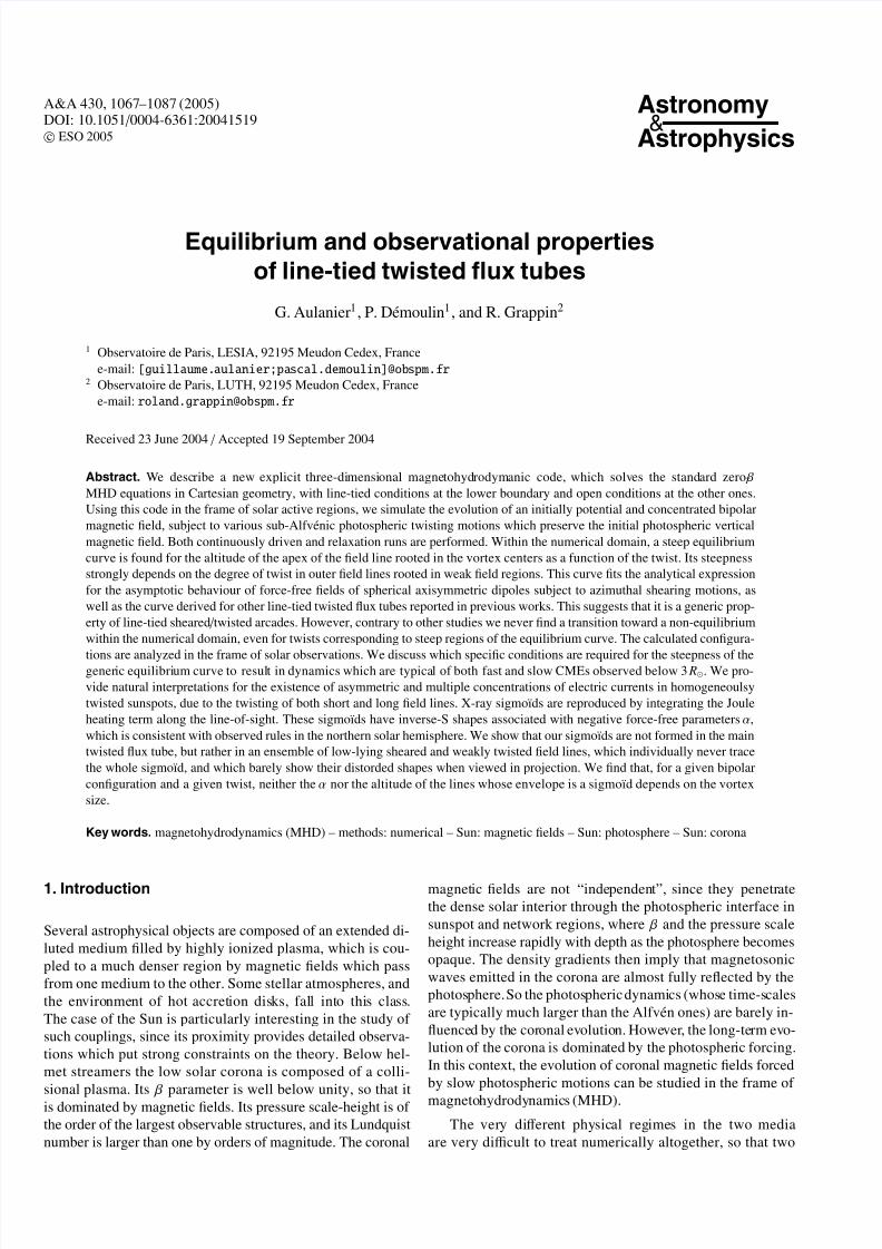
Fig. 1. Magnitude of the initial potential magnetic field versus altitude

at the center of the domain at ( x; y) = (0;0).

the Fourier code developed by Démoulin et al. (1997) which is

periodic in ( x; y). The extrapolation is done with N x × N y =

10242 points uniformly distributed on the ( x; y) plane with

( x; y) ∈ [−200 Mm; 200 Mm]. The extrapolation results in

a magnetic field decrease with z which is plotted in Fig. 1.

In order to calculate an open rather than a periodic sys-

tem in our MHD runs, a domain D is extracted from the

periodic domain used in the extrapolation. In the following,

we consider D in ( x; y) ∈ [−100 Mm; 100 Mm] and ( z) ∈[0 Mm; 200 Mm]. Using linear interpolations between the

gridpoints of the Fourier extrapolation, the magnetic field val-ues are saved on a non-uniform mesh with n x × ny × n z =

2013 points. The smallest cells are concentrated around x =

y = z = 0, on top of the inversion line of b z( z = 0) where

(b x; by) are the strongest at t = 0. The mesh intervals vary

in the range (d x; dy; d z) ∈ [0.2 Mm; 2.8 Mm], expanding

from x = y = z = 0 following d i+1 x /d i x = d

j+1y /d

jy = 1.027

and d k +1 z /d k

z = 1.013. The resulting potential field is shown in

Fig. 2.

As a result of the extrapolation, the ratio of the maximal

to the minimal value of b in D is about 5 × 103. In order

to mimic (1) the filling of plasma in coronal loops rooted in

strong field regions, (2) the coronal density decrease with alti-tude and (3) the fact that the Alfvén speeds cA always remain

much larger in the corona than the photospheric driving veloc-

ities, we prescribe the ad-hoc initial density in D:

ρ( x; y; z; t = 0) = ( µ c◦)−1 b2( x; y; z; t = 0), (36)

so that cA( x; y; z; t = 0) = c0 = 103 km s−1. In all our runs,

we find that local magnetic field and density variations result

in Alfvén speed variations roughly between 0.7 and 5 c0. These

settings and Eq. (25) result in timestep values of 0.01 < dt (s) ≤0.1.

3.2. Procedure for boundary driving

We apply a horizontal divergence-free boundary driving of the

field line footpoints at z = 0 so as to kinematically twist the




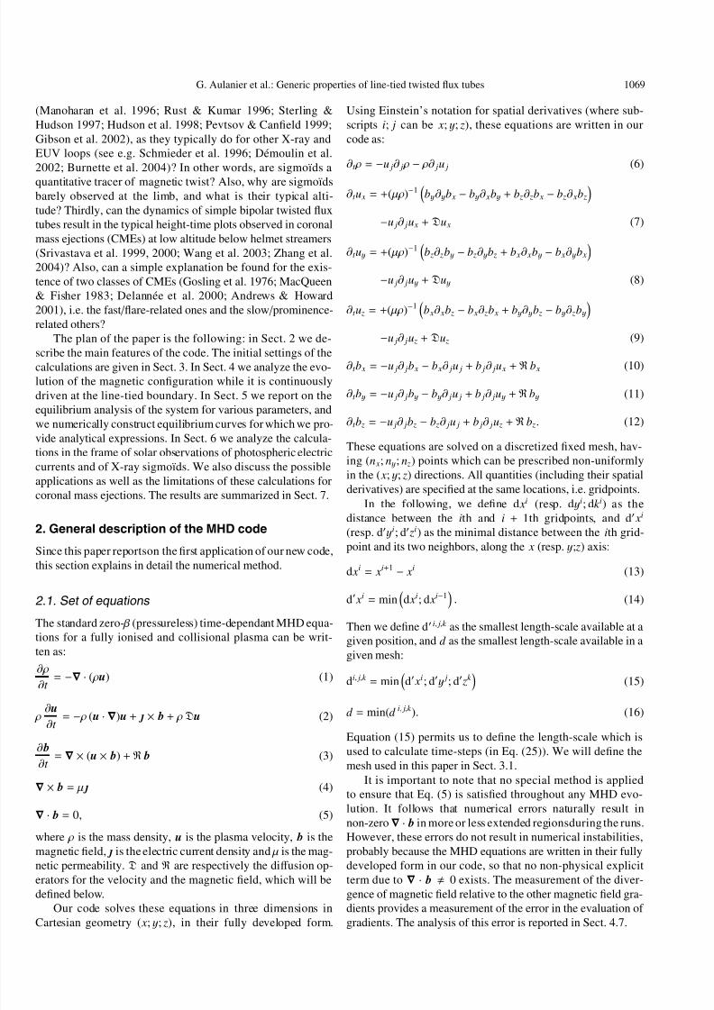
Fig. 2. Top and projection views of the initial potential magnetic field within the whole domain. The grey scale at the z = 0 plane is white / black

for b z = ±480 G. [Pink; red; green; dark-blue; light-blue; black] field lines are rooted in b z = ± [475; 400; 300; 250; 150; 50] G.

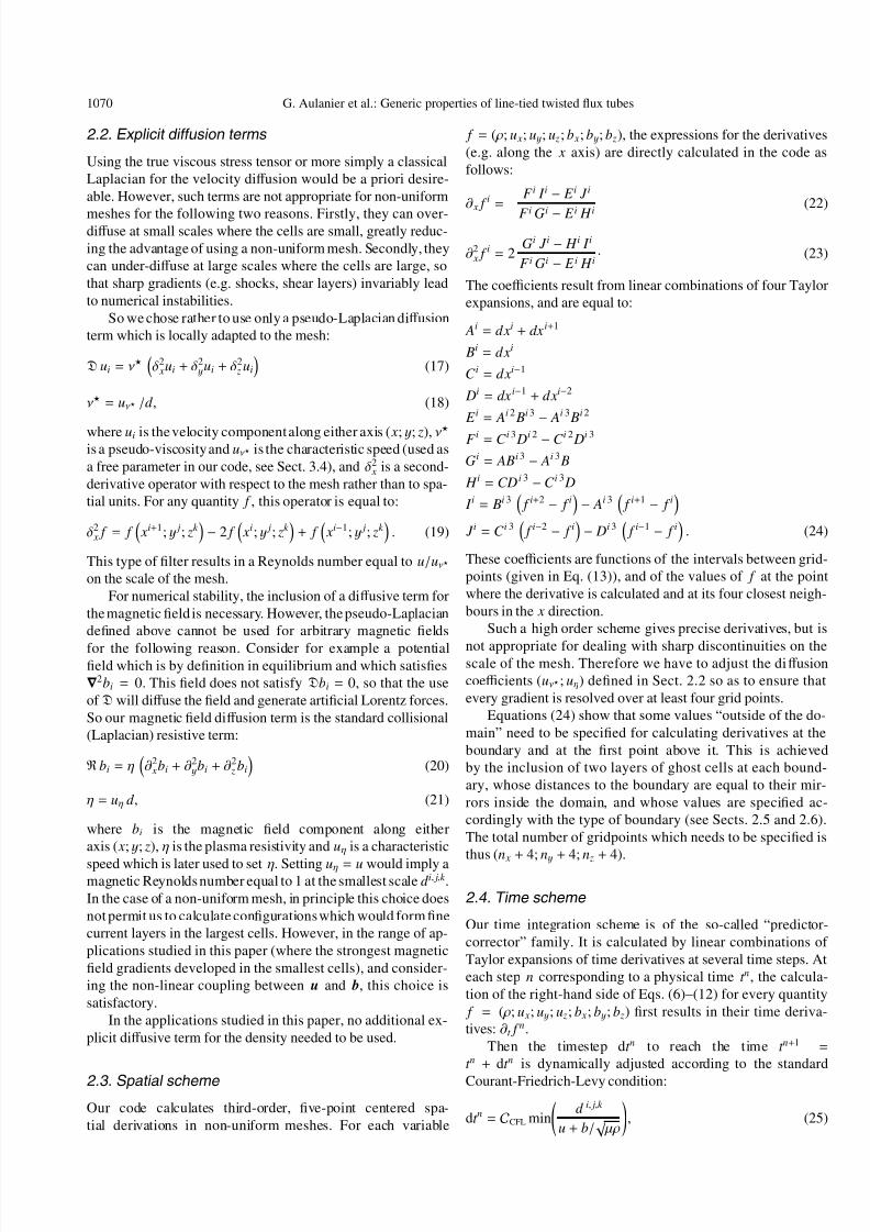
Fig. 3. (First row): Profiles of b z and uy along the ( x; y = 0, z = 0) axis. (Second row): Contours of b z = ±50; 100; 150; 200; 250; 300; 350;

400; 450 G and velocity vectors at z = 0. The [first;second;third] columns correspond to vortices defined by ζ = [10;0.9; 0.5].

initial potential configuration. We choose a velocity field which

preserves the initial distribution of b z( z = 0), so that the mini-

mum magnetic energy remains the same during all runs, i.e. the

energy of the potential field at t = 0. In this context, Eq. (12) at

z = 0 turns into:

∂t b z = −∇⊥ · (b z u⊥) (37)

where u⊥ = (u x; uy) and ∇⊥ = (∂ x; ∂y). Eq. (37) then implies:

u⊥ = ∇⊥ ψ(b z; t ) × e z, (38)

where e z is the unit vector along the z axis and ψ(b z; t ) is an

arbitrary potential which only depends on b z and on time. In all

our runs we choose the same potential as Amari et al. (1996)

and Török & Kliem (2003):

ψ(b z; t ) = ψ◦ γ (t ) b2 z exp

b2

z − bmax 2 z

ζ 2 bmax 2 z

, (39)

where γ (t ) is a ramp function giving an initial acceleration to-

ward a constant twisting velocity:

γ (t ) =1

2tanh

2(t − t α)

t ω

+

1

2· (40)




This function results in two vortices centered around the max-

ima of |b z( z = 0)| for which the horizontal velocity vectors are

tangential to the contours of b z( z = 0). In our runs, we fix ψ◦so that u

max⊥ = 20 km s−1 = 0.02c0. The middle of the ramp

function is at t α = 300 s and its half-width is t ω = 100 s. This

ramp function allows the system to find a good numerical equi-

librium before t = 200 s, when the acceleration begins. ζ is

a free parameter which controls the physical extension of the

vortices. Even though this boundary driving analytically pre-

serves b z( z = 0), it numerically results in small deformations

of b z( z = 0) contours in the vicinity of the vortex centers. In

order to ensure that b z( z = 0) is conserved in our runs, it is

numerically re-enforced at each time-step.

In order to study the dependence of the system on the size

of vortices, we performed three sets of runs, with ζ = 10;

0.9; 0.5. The first case results in extended vortices which twist

most of the flux and which shear the inversion line, the third

case results in concentrated vortices which twist only thestrongest fields, and the second case is intermediate. The as-

sociated velocity fields are shown in Fig. 3.

3.3. Procedure for relaxation runs

Even though the applied boundary driving is very slow (2% of

the Alfvén speed), the continuously twisted runs always end

up after some time in velocities of the order of cA (see Sect. 4).

This indicates that the system is far from equilibrium.

In order to find an equilibrium (or to reveal its absence)

for a given amount of twist reached at a time t , we perform

relaxations runs as follows. Time is reset to zero, the magneticfield and mass density are set to [ b; ρ](t = 0) = [ b; ρ](t = t ),

the boundary driving is suppressed (ψ◦ = 0) and the velocities

are reset to u(t = 0) = 0. So the further evolution of the system

is only driven by the residual Lorentz forces which exist at t =

t during the continuously driven run.

This method is more demanding numerically than apply-

ing a gradual deceleration of the driving at z = 0 while keep-

ing its velocities in D. However, it is more convenient be-

cause the amount of twist is fixed during the relaxation (if uη

is small enough), and essentially because velocities resulting

from the accumulation of momentum during the driven phase

do not play a role in the evolution of the system. This issuebecomes important when the velocities are of the order of the

Alfvén speed.

3.4. Diffusion parameters

In order to avoid the formation of unresolved strong shear lay-

ers at high altitudes z, which naturally appear due to prescribed

motions at the footpoints of strongly expanding flux tubes, we

apply a strong diff usion term foru: uν = 150kms−1. However,

to ensure a high magnetic Reynolds number in the corona, we

set a much smaller diff usion term for b: uη = 15 km s−1.

Estimating (i) the typical length-scale as 30 Mm, which isroughly equal to the initial length of the magnetic field line

rooted in bmax z ( x; y; z = 0) as well as the average transverse ex-

tension of the twisted flux tube which forms in our runs; and

(ii) typical velocities as 0.1c0, the characteristic dimensionless

numbers are ( Re; Rm; Lu) = (102; 103; 104). The value of the

Reynolds number here is only an upper limit, since the vis-

cous term is defined at the scale of the mesh in our code (see

Eq. (17)).

The diff usion velocities (uη; uν ) are kept constant in space

and time, and are the same for every run (continuously driven,

relaxation and varying ζ ).

4. Results from the continuously twisted runs

4.1. Twist definition and maximum values

During the continuous photospheric driving, field lines rooted

in the prescribed vortices start to twist around the “axial field

line” which is rooted in bmax z at the vortex centers. Figure 4

shows that both the magnetic and kinetic energies increase

monotonically for the three vortex sizes considered (ζ =10;0.9; 0.5) as long as the boundary driving is maintained.

The kinetic energy for the small vortices naturally remains

smaller than the one for large vortices, since the coronal vol-

ume at z > 0 which is aff ected by the vortices depends on the

vortex size.

Since the three vortices have diff erent sizes, but with the

same maximum velocity and initial acceleration ramp, they

have diff erent rotation rates around the axial field line. So in

the following, we study the variation of all quantities as a func-

tion of twist Φ rather than time, so as to have a common time-

scale. Φ is calculated analytically, and also checked numeri-

cally at various timesteps by integrating many magnetic field

lines along the x axis for ( x < 0; y = 0; z = 0) and by measur-

ing the rotation rate of their footpoints at ( x > 0; z = 0). We

find that the prescribed motions result in a nearly rigid rotation

inside a small radius Rphot 1.5 Mm around the vortex centers,

which gradually decreases away from them. The twist unit Φ

which we consider in the rest of the paper is the rotation angle

of the field line footpoints in the small area which is subject

to a quasi-rigid rotation. We define the number of turns in the

associated magnetic flux tube by N = Φ/2π.

For the three vortex sizes considered, the results of the

calculations are only shown up to twists equal to N max =

(1.22;1.61;1.66) turns for ζ = (10;0.9; 0.5) for the following

reasons. The physical meaning of the runs is indeed boundedby two limitations. Firstly, the most relevant field lines (those

anchored in strong field regions) can reach (and then cross)

the top boundary of the domain, which prevents communica-

tion via Alfvén waves between their footpoints at z = 0. This

limitation comes up for ζ = 10 when N > N max, during con-

tinuously driven runs, and for ζ = 0.9 when N > 1.48 dur-

ing relaxation runs (see next subsections). Secondly, a current

shell develops in all runs for z ≥ 0 at the interface between the

strongly and weakly twisted field lines : this shell must remain

numerically resolved. For ζ = 0.5 the shell becomes unresolved

for N > 1.70, simply because the vortices are more concen-

trated than in the other runs. This leads to numerical instabili-ties which start to develop around ( x; y; z) = (±9; ±17; 30) Mm,

where the cell intervals (defined by Eq. (13)) are (d x; dy; d z) ∼(0.3; 0.6; 0.6) Mm. Increasing the resistivity makes it possible




Fig. 4. Continuously twisted runs. All quantities are plotted as a function of the central twist

N . Each mark is separated in time by ∆t = 30 s.

[stars; pluses; crosses] correspond to ζ = [10;0.9; 0.5]. (First row): Global magnetic and kinetic energies. (Second row): Altitude and verticalvelocity of the axial field line rooted in the vortex centers.

to bypass this problem. However, we did not go on in this di-

rection, because comparison with other runs would have been

difficult.

4.2. Quasi-static phase

During a first long quasi-static period, in the strongest and

closed field regions, the slow velocities of the photospheric

driving allow the low frequency Alfvén waves which are gener-ated at z = 0 by the vortices to travel several times along a given

field line by rebouncing on the line-tied plane at z = 0. This

leads to a smooth distribution of the generated electric currents

along each magnetic field line. This allows the magnetic con-

figuration to remain close to a non-linear force-free state. This

was checked by integrating both electric current and magnetic

field lines, which become undistinguishable from one another

after a short transition phase after the start of the runs. In the

outer “open” field lines rooted in weak field regions (which

emerge out of the numerical domain) the waves are trans-

mitted through the open boundaries with very little reflexion,

thanks to the dissipative operator for the velocity applied on thenon-uniform mesh. However, since these field lines are also

continuously twisted, they do not come back to a potential

state.

The whole magnetic configuration slowly expands in all di-

rections, but mostly along z. This can be explained in the con-

text of the van Tend & Kuperus (1978) model by the genera-

tion of surface currents at the infinitely conducting and inertial

plane at z = 0, which tend to expell the generated coronal cur-

rents away from them, and by the self-repulsion of the coronal

currents for z > 0. This can also be explained by the fact that

since b z( z = 0) remains constant, the currents at z > 0 generated

by the twisting motions at z = 0 result in a global increase of

magnetic energy, hence in local enhancement of magnetic pres-sure within the twisted flux tube, so in local expansion where

the magnetic tension does not increase as fast as the magnetic

pressure. During this quasi-static phase, the twisting flux tube

expands with a vertical velocity u z which is smaller than the

boundary driving maximal velocity. This first phase lasts until

the accumulated vertical velocities become of the order of 5%

of the Alfvén speed, i.e. u z = 50 km s−1, which is nearly equal

to the sum of the two vortex velocities, which is about the maxi-

mum amplitude of the torsional Alfvén wave propagatingalong

the loop.

4.3. Dynamic phase

A second phase of dynamic nature then begins. The rates of in-

crease for u z, for the kinetic energy and for the apex altitude of




the axial field line gradually rise to much stronger values than

during the quasi-static phase. This smooth transition does not

occur for the same twist for all vortex sizes. Figure 4 shows that

the change occurs for central twists of N ∼ 0.5; 0.7; 1.0 turns

respectively for ζ = 10;0.9; 0.5. As the twist increases, the ki-

netic energy gains one order of magnitude, and the vertical ve-

locity of the axial field line reaches a non-negligible fraction of

the Alfvén speed. For a given twist the vertical velocity of large

overlaying field lines is even higher (but always sub-Alfvénic

in our runs): these large field lines are pushed upward and side-

ward together, both due to their own internal currents and to the

pushing from below by the more twisted flux tube. Analyzis of

the height-time curves for the axial field line reveals an expan-

sion rate which is slightly faster than exponential. During this

second phase the magnetic field configuration becomes less and

less force-free, as indicated not only by the very fast expansion

velocities, but also by an increasing angle between the electric

current and the magnetic field lines.Regardless of the existence or not of a non-equilibrium,

the observed departure from the force-free state is expected.

Indeed, the vertical expansion results in longer and longer field

lines. The rate of increase of field line length becomes such that

the low frequency Alfvén waves emitted from the photospheric

boundary at z = 0 no longer have time to rebounce several

times along a given field line, so that the currents cannot be

quasi-statically distributed all along the field line. This results

in a system which is always trying to reach an equilibrium (if

any) that is located at larger and larger heights in z as the twist

increases.

As the twist increases, the core twisted flux tube emergesout the numerical domain at a rate which is faster than ex-

ponential, with velocities of the order of the Alfvén speed.

Meanwhile, the surrounding twisted and potential loops lean

sidewards. This whole behaviour described above is qualita-

tively the same for all three vortex sizes considered in this

paper. It is also fully consistent with what was reported for

other classes of bipolar twisted fields calculated by Amari

et al. (1996) and Török & Kliem (2003) with diff erent zero- β

MHD codes. Consequently, we conclude that the “very fast

opening” initially reported by Amari et al. (1996) is a generic

property of continuously twisted bipolar line-tied flux tubes.

4.4. Influence of the weak field regions

The comparison of the height-time plots for the three vortex

cases during both quasi-static and dynamic phases shows that

the vertical expansion rate of the axial field line is much larger

for large than for small vortices. The dependence on vortex size

is much larger than linear. Since the outer field lines are twisted

more by the large vortices, we interpret the above result as in-

dicating that the degree of twist in the outer field lines has a

large influence on the expansion rate of the strong fields.

This can be qualitatively explained by the expansion of the

outer field lines under the action of their own internal currents,which adds up to pushing from below due the twisted flux tube

expansion. Quantitatively, the high sensitivity to the vortex size

may be associated with the behaviour of large field lines in

constant-α linear force-free field models, whose distortion and

expansion rates are typically much larger than those of low-

lying field lines for small increments of α, as explained below.

In ( x; y) periodic linear force-free field models, the mag-

netic field amplitude varies with z as b( z) ∝ exp(− z √ k 2

− α2

)where k = 2π/ L is the wavenumber of the considered Fourier

mode (see e.g. Aulanier & Démoulin 1998). This readily shows

that low-wavenumber modes (i.e. large field lines) are much

more aff ected by α variations (i.e. by injection of electric cur-

rents) than high-wavenumber modes.

Even though this explanation cannot be directly transposed

to the present MHD calculations since they result in non-

constant α distributions and in departures from the force-free

state, we believe that it is at the origin of the strong depen-

dence of the system on the twisting (or not) of large outer field

lines.

4.5. Inclination and reorientation of the field lines

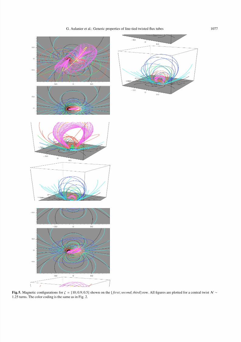
Figure 5 shows the structure of the magnetic configuration for

the three vortices at the same twist during the dynamic phase.

These figures show the sideward inclination of the field lines

which surround the twisted core (drawn with pink field lines)

and which are rooted in weak field regions on the edge of the

photospheric bipole. This behaviour is similar to what Amari

et al. (1996) reported.

A re-orientation of the core twisted flux tube is also evident,

as found in the calculations of Török & Kliem (2003). We find

that this flux tube makes an angle with its initial orientationalong the x axis, which scales like the vortex size. However,

this re-orientation is neither associated to the dynamic phase

nor to some kink-like instability, since it is already noticeable at

N ∼ 0.5 N during the quasi-static phase. This phenomenon is

in fact simply caused by the swirling of initially low-lying field

lines having strong transverse fields which cross the inversion

line. This swirling results in the increase of magnetic pressure

along the y axis at low altitude on one side of a given vortex.

This pressure term is not present on the other side of the vortex

since the corresponding larger field lines are relatively less de-

formed by the vortex. The pressure imbalance pushes the lower

parts of the flux tube sideward from the x axis, and this defor-

mation propagates to larger heights along each field line thanks

to Alfvén waves, which results finally in the deformation of the

whole twisted flux tube.

4.6. Behaviour near the top boundary

When the core twisted flux tube, which is associated with the

strongest volumic currents, gets close to the top boundary,

it keeps accelerating even though the acceleration diminishes

(see Fig. 4 for the run with ζ = 10). The apex of flux tube

eventually always passes through the top boundary, just like

some surrounding field lines rooted in weak field regions do atsmaller times. The decrease of acceleration when the axial field

lines passes z ∼ 175 Mm is probably not physical, this altitude

being only at 9 mesh points from the boundary.




Fig. 5. Magnetic configurations for ζ = [10; 0.9; 0.5] shown on the [ first ; second ; third ] row. All figures are plotted for a central twist N ∼1.25 turns. The color coding is the same as in Fig. 2.




Fig. 6. Five examples of relaxation runs. Pluses correspond to (N = 1.05; ζ = 10), stars to (N = 0.92; ζ = 10), diamonds to (N = 1.48; ζ = 0.9),

triangles to (N = 1.41; ζ = 0.9) and crosses to (N = 1.66; ζ = 0.5). Each mark is separated in time by ∆t = 30 s. ( Left ): Magnetic energy as a

function of time. ( Right ): Altitude-velocity diagrams showing the begining of damped oscillations along z.

vertical component of the Lorentz forces, which eliminates

a pure diff usive origin. Also, performing relaxations with in-

creased resistivity by a factor 3 has not led to qualititative

changes.

So we conclude that the system always enters an oscilla-

tory behaviour along a potential well around an equilibrium

position. These oscillations result from the initial position of

the flux tube away from the equilibrium point at the start of the

relaxation, so that inertia allows the system to pass beyond this

point, which is followed by the action of restoring forces which

pull back the system toward the equilibrium. The existence of

these oscillations obviously shows that the system is not over-diff usive, in spite of the strong value of uν which we chose in

Sect. 3.4.

Comparing various relaxation runs, we find that the ini-

tial vertical acceleration, the peak vertical velocities and the

amplitude in z of the oscillations for a given vortex size are

all larger as the relaxation is performed for higher and higher

twists N . This indicates that the system proceeds further and

further away from its equilibrium position as N increases

during the dynamic phase of the continuously driven runs.

However, our calculations suggest that the system can always

find an equilibrium.

5.2. Comparison with other authors

The rapid increase of expansion rate of the equilibria as

function of footpoint displacement that we find is consis-

tent with other numerical calculations of twisted bipoles in

Cartesian geometry by Amari et al. (1996), Klimchuk et al.

(2000) and Török & Kliem (2003), as well as with the be-

haviour of axisymmetric sheared dipoles in a spherical geome-

try (Roumeliotis et al. 1994). Our relaxation behaviour is con-

sistent with Amari’s qualitative statements and with the results

of Klimchuk et al. (2000), about the increasing difficulty in re-

laxing the system for increasing twists. However, contrary toTörök & Kliem (2003), we find no evidence for a loss of equi-

librium in any of our systems, even though their bipolar field

resized to our scale results in a loss of equilibrium when the

altitude their axial field line is less than ∼40 Mm, which is

much smaller than the vertical extension of our domain.

This quantitative diff erence may be due to diff erent numeri-

cal prescriptions between codes. Firstly, Török & Kliem (2003)

apparently use a much stronger diff usion term for momentum

(and for density) than we do, since their “successful relaxation”

runs apparently do not show oscillatory behaviour. Secondly,

they use a non-uniform grid which is typically 3.3 times more

stretched in z than ours for similar altitudes, if their spatial units

are rescaled to ours to have the same bipole size at z = 0 (Törok

2004, private communication). Thirdly, they use a diff erent spa-

tial scheme than we do. Fourthly, the development and conse-quences of non-zero ∇ · b in their runs must be diff erent than

in ours. Indeed, they use the standard conservative form of the

MHD equations. Finally, their boundary conditions at z = 0

on b are not the same as ours, even though their b z( z = 0)

varies only slowly with time. All these issues may result in

diff erences in the calculation of spatial derivatives, hence of

Lorentz forces.

The analysis in our relaxation runs of each term that con-

tributes to the vertical acceleration in Eq. (9) shows that, around

the time at which we find a deceleration, and around (and

above) the altitude of the axial field line, the vertical derivative

term by∂ zby is well resolved, and is at most 10 times larger thanthe total vertical component of the Lorentz force. A small dif-

ference in the calculation of this term, which may be amplified

in time, may result in a diff erent sign for the vertical Lorentz

force. This issue will have to be addressed by new calculations

in the future, if possible with diff erent codes.

5.3. Analytical equilibrium curve

In order to derive the precise numerical equilibrium curves for

our three vortex sizes, we need in principle to perform pro-

hibitively long relaxation runs so as to follow the damping of

the vertical oscillations of the magnetic field. We rather choosea simplified method. We measure the altitude in z of the axial

field line at the time for which the vertical acceleration first be-

comes negative during the relaxations (see Fig. 6). Since this




Fig. 7. Equilibrium curves derived from relaxation runs. ( Left ): Same as Fig. 4, bottom left , overlaid with [triangles; diamonds; squares] which

correspond to “equilibrium” positions found from relaxation runs with ζ = [10;0.9; 0.5]. The corresponding equilibrium curves are overplotted

as dashed lines. ( Right ): Same equilibrium curves and calculated “equilibrium” positions plotted with log / square axes. The dashed horizontal

line represents the height of the top boundary.

time is well matched in our runs by the change in sign of the

vertical component of the Lorentz force, we then assume that

this altitude corresponds to the asymptotic equilibrium of the

system. The measured positions for various values of (N ; ζ )

are marked in Fig. 7, left on top of the height time plots from

the continuously twisted runs. The equilibrium positions for a

given twist are always located above those found when the sys-

tem is continuously twisted. As conjectured in Sect. 4.3, this

can be explained by the fact that the currents continuously gen-

erated by the vortices at z = 0 do not have time to distributeall along the expanding field lines by Alfvén waves, especially

during the dynamic phase during which the expansion rate is

comparable to the Alfvén speed.

We find that these positions are well aligned in Fig. 7, right ,

in accordance with the “successful relaxation” plots of Török

& Kliem (2003) which were calculated for diff erent physical

conditions with a diff erent code (recall in particular our approx-

imate relaxation method and our problems with the ∇ · b con-

straint). For comparison, the three curves which link the marks

calculated for all three ζ values are overplotted onto Fig. 7, left .

So we find that all our equilibrium curves follow the analytical

expression:

h(N ) = h◦ expA N 2

, (42)

where h is the altitude of the axial field line at a given twist N ,h◦ is the altitude of this field line for the potential field and Ais a geometrical factor which, for a fixed initial potential field,

depends on ζ i.e. on the vortex sizes.

Our numerical reconstructions of these curves show that

for ζ = (10;0.9; 0.5), A (2.16;1.12;0.50). By comparison,

Török & Kliem (2003) find A 0.75 before their flux tube

loses its equilibrium. This value lies within the range of Awhich we found. Also it is now clear that our magnetic con-

figuration always enters an oscillatory stage during its relax-ation, even when the equilibrium curve is steeper than the one

of Török & Kliem (2003). Both these issues suggest a poste-

riori that their loss of equilibrium is not be physical, and that

simple bipolar twisted flux tubes can always evolve quasistati-

cally if the photospheric driving velocities are infinitesimal.

As noted by Török & Kliem (2003), the analytical equilib-

rium curve given in Eq. (42) also applies to other geometries,

specifically to spherical axisymmetric (2.5D) dipoles subject to

azimuthal shearing motions (Roumeliotis et al. 1994; Sturrock

et al. 1995). The derivation of this curve by both analytical and

numerical means, by several authors and in various geometri-

cal conditions, implies that it is a generic property of line-tied

force-free fields, both sheared and twisted.

6. Observational properties

6.1. Coronal mass ejections

In the following we address the question of the applicability of

the continuously twisting bipolar flux tube model to the coronal

mass ejection (CME) phenomenon. We assume that the analyti-

cal expression of the equilibrium curve (Eq. (42)) remains valid

with altitude until the apex of the axial field line reaches the

top of helmet streamers, where the solar wind becomes domi-

nant (i.e. 2−3 R). We also assume a photospheric twisting rateN (t ) = uphot/(2π Rphot), where uphot is the twisting velocity and

Rphot is the radius of the small region which defines the twist

within each vortex ( Rphot = 1.5 Mm for h◦ = 11.5 Mm, see

Sect. 4.1). Equation (42) then leads to:

h(t ) = h◦ exp

A

uphot t

2π Rphot

2, (43)

v z(t ) = 2 A t

uphot

2π Rphot

2

h(t ). (44)

These analytical expressions should in principle be recoverednumerically in the limit of infinitesimal photospheric twisting

velocities. Figure 8 shows some corresponding plots using two

values of (h◦; Rphot) scaled by the same factor f (one typical of




Fig. 8. Simulated height-velocity-time plots of the axial field line

of continuously driven flux tubes twisted with uphot = 1 k m s−1,

for altitudes between the photosphere ( z = 1 R) and the top of

helmet streamers ( z = 2−3 R). [thick ; thin] lines correspond to

h◦ = [11.5; 69] Mm and to Rphot [1.5;9] Mm. [dash-dotted ; contin-

uous; dashed ] lines correspond to ζ = [10;0.9; 0.5].

the size a young active region and another typical of a promi-

nence) and three values of A (corresponding to the three vortex

sizes calculated in this paper).

Regardless of the velocity magnitudes, Fig. 8 illustratesone typical property of Eq. (42): the scale dependence. It is

clear that the system size (i.e. prominence as opposed to ac-

tive region) scales inversely with the acceleration and to the

velocities. In particular, the velocity (resp. acceleration) at

h h◦ roughly scales like f −1 (resp. f −2). All these prop-

erties are consistent with the two classes of observed CMEs

(Gosling et al. 1976; MacQueen & Fisher 1983; Delannée

et al. 2000; Andrews & Howard 2001): the fastest (resp. slow-

est) ones mostly originate from active regions (resp. quies-

cent prominences), and once they reach the inner edge of the

SoHO / LASCO coronographs, they typically have radial veloc-

ities of the order of 500–1500 km s−1 (resp. 50–300 km s−1).As

in the flux rope model of Chen & Krall (2003) which considers

end-to-end twists of about 4 turns (Chen 2004, private commu-

nication) the present explanation for both classes of CMEs is

based on the size diff erence between prominences and active

regions. However, contrary to Chen & Krall (2003), our model

does not involve the evolution of the flux tube curvature dur-

ing a free expansion, but rather a direct scaling e ff ect of the

equilibrium curve during a driven expansion.

The velocity magnitudes in Fig. 8 have been calculatedfor a photospheric velocity of 1 km s−1 so as to obtain typi-

cal CME velocities at 3 R. Even though the observed dynam-

ics of CMEs have typically been studied at greater heights, a

few height-velocity-time plots have been measured at lower al-

titudes (Srivastava et al. 1999, 2000; Wang et al. 2003; Zhang

et al. 2004). Even though these observed plots appear to be in

qualitative agreement with Fig. 8, two strong diff erences must

be emphasized. Firstly, the prescribed uphot is at least ten times

larger than photospheric velocities typically observable in ro-

tating sunspots (Brown et al. 2003, and references therein).

Secondly, the initial “quiet phase” before the “very fast open-

ing” is not longer than a few hours (resp. a day) for the active

region (resp. prominence) case. This is much too small com-

pared to observed time-scales which are of the order of days to

weeks.

The only way to bypass the first difficulty (too fast pho-

tospheric flows) would be to have twist either injected by re-

connection rather than by flows, or by fast undetectable flows

within sunspots due e.g. to twisted flux emergence through the

photosphere. The second issue (too short quiet phase) would

imply that twist is not injected continuously, but rather in

episodic bursts well related with the launch of CMEs, with

time scales of the order of a few hours to one or two days.

Direct application of this model to the CME phenomenon thus

requires the same artificially fast twisting as in the analyticaldriven model of Chen (1996).

However, as emphasized by Forbes (2001), “this point of

view is difficult to reconcile with the extremely tranquil con-

ditions that exist in the photosphere during flares and CMEs”.

In our opinion, since the dynamic evolution of the weak fields

surrounding the core twisted flux tubes plays a very important

role in the dynamics of the system for twist values ≥1 turn (see

Sect. 4.4), their global reconfiguration associated with e.g. dis-

tant flux emergence (Lin et al. 2001) and / or magnetic recon-

nection (Antiochos et al. 1999) is most likely to lead to a CME.

In the frame of our model, such reconfigurations may be asso-

ciated with dynamic changes of the value of the parameter Ain Eq. (42), which may solve the problem of the speed of the

twist injection encountered by the present model and in Chen

(1996).




Fig. 9. (First row): Contours of b z = ±50;100; 150; 200; 250; 300; 350; 400; 450 G and transverse field vectors at z = 0. (Second row): Greyscale

images of z at z = 0. White / black correspond to z = 9 mA m−2. The [first; second; third] columns correspond to vortices defined by

ζ = [10;0.9; 0.5]. All figures are plotted for a central twist N ∼ 1.25 turns.

6.2. Photospheric electric currents

We calculate the vertical electric current densities from the

photospheric transverse fields,

z = µ−1∂ xby − ∂yb x

, (45)

which result from the MHD evolution of the initial potential

field subject to all three vortex sizes considered in this paper.

Both are plotted in Fig. 9 for a central twist of N ∼ 1.25 turns.

Some generic properties are found in all three cases, and are

discussed below.Within each magnetic polarity, both direct and surround-

ing return currents co-exist. The extended weak return currents

naturally form by shearing / twisting an initial line-tied potential

field, so as to maintain the outer untwisted fields potential. The

direct currents are more concentrated and intense. Their max-

imal values are about | z| ∼ 6−9 mA m−2 for the largest and

the smallest vortex sizes respectively. If the magnetic field am-

plitudes of the bipole were scaled to those of typical sunspots

(bmax z = 2000 G instead of 480 G), these currents would be

| z| ∼ 24−36 mA m−2, in accordance with typical vector field

measurements within sunspots (see e.g. Pevtsov et al. 1995;

Leka & Skumanich 1999; Régnier et al. 2002).These currents correspond to a negative value of the force-

free parameter α which is defined as α = µ zb−1 z . This sign is

consistent with the prescribed boundary motions, which result

in a left-handed magnetic twist, so a global negative magnetic

helicity. For all three cases the maximum values are nearly the

same: α ∼ −0.25 Mm−1. This is so because the more concen-

trated the vortex, the higher z and the higher b z at the location

of these strong currents (see Fig. 9). So the typical scale-length

L = 2πα−1 25 Mm of the strongest current-carying field lines

is the same for all three cases.

This α value is typically 15−30 times larger than what is

found in linear force-free field models of large-scale loops in

sheared active regions (Schmieder et al. 1996; Démoulin et al.2002). It is also 5−10 times larger than in models of interme-

diate and plage prominences (Aulanier & Démoulin 2003) and

X-ray sigmoïds (van Driel-Gesztelyi et al. 2000; Gibson et al.

2002). Note that in these past works, α was calculated for typ-

ically 2−8 times larger configurations than those studied here.

So the present rescaled α values fall in the range of those esti-

mated for prominences and sigmoïds.

Another generic property is a strong azimuthal asymmetry

of the distribution of the transverse fields and of z with respect

to the vortex centers (compare Figs. 3 and 9). Consider one

magnetic polarity, e.g. for x < 0. Firstly, the apparent vortex

centers as deduced from the transverse fields are always shiftedfrom the real vortex centers located at bmax z . Secondly, the trans-

verse fields originate radially from the vortex centers in a quad-

rant ( x < xc; y < yc), where ( xc; yc) are the coordinates of the




left vortex. On the contrary, the transverse fields tend to follow

the contours of b z for another quadrant ( xc < x < 0; y > yc).

Thirdly, z shows a swirling pattern around ( xc; yc). Several spi-

ral arms of opposite signs for z and of various widths appear

for

N > 0.5 turn, and develop more and more with time as the

twist increases.

This azimuthal asymmetry is not present in cylindrical

MHD calculations in which both extremities of the cylinder

are line-tied. It is a geometrial property caused by the curva-

ture of the field lines which are line-tied onto the same plane.

This asymmetry comes from the fact that, even though the same

amount of twist Φ is injected for both short field lines (rooted

on each side of the inversion line around x = 0) and large ones

(located on the edges of the bipole), stronger currents are gen-

erated in the smaller field lines. This can be explained by con-

sidering a simple cylindrical flux tube model in (r ; z; φ), where

l is the length of the flux tube along z. The electric current and

field line equations in cylindrical coordinates result in:

z = r −1∂r (rbφ) ∝ bφ (46)

bφ = rl−1b zΦ. (47)

It naturally follows that for (r , Φ) fixed, shorter field lines (hav-

ing small l) will contain stronger currents since z ∝ l−1. As the

twist proceeds, relatively stronger currents are generated near

the footpoints of the initially shorter field lines, resulting in an

asymmetry not only in x, but also in y. This eff ect is even more

amplified by the expansion of the large field lines with increas-

ing twist (including the core twisted flux tube): this expansion

is faster than the expansion of the smaller field lines. This am-

plification is then partly responsible for the gradual inclusion of

the weak return current region within the swirling pattern of zdescribed above, around the footpoints of the fast expanding

core twisted flux tube.

Interestingly, the complex asymmetric structure of z in the

photosphere is formed within a very simple magnetic config-

uration which is initially smooth, bipolar and symmetric, and

which is twisted by vortex motions that are also very simple.

Also, this structure qualitatively remains very similar for ex-

tended as well as concentrated vortices. So it is probably a

generic property of line-tied twisted flux tubes rooted in the

photosphere. It follows that twisted sunspots should naturally

have – at least – two more-or-less contrasted concentrations of strong direct electric currents within a given magnetic polarity,

and possibly – at least – one patch of weak return current of

opposite sign. This is in very good agreement with the obser-

vations (Pevtsov et al. 1995; Leka & Skumanich 1999; Régnier

et al. 2002). In the frame of our model, the observed fragmen-

tation of the force-free parameter α within sunspots is then not

necessarily due to some hidden complexity in the distribution

of the photospheric flux or of the footpoint twist.

6.3. X-ray sigmoïds

A common assumption for the materialization of observed so-lar structures is that they are directly traced by magnetic field

lines. However, it has already been shown for the case of

filaments and prominences that this assumption is not fully

valid, and that only portions of field lines trace the visible fea-

tures, both in Hα and in EUV wavelengths (e.g. Aulanier &

Schmieder 2002). In the following we address the validity of

this assumption for sigmoïdal structures observed in X-rays.

Our main hypothesis is that since X-rays make it possible to

visualize the hottest parts of the corona, the observed intensity

I X-rays is nearly proportional to the Joule heating term integrated

along the line of sight. If we consider the bipole to be at the

disc center for simplicity, we simulate X-ray observations by

calculating:

I X-rays( x; y) ∝

2( x; y; z)d z. (48)

This assumption is very approximate since the energy equation,

whose proper treatment would imply very short timescales,

is not integrated in our present calculations. In particular, the

issue of thermal conduction along heated field lines, whichcan result in their filling by dense material originating from

chromospheric evaporation, is not considered. Keeping this

limitation in mind, we analyze the results of the simulated

X-ray observations for all three vortices at the same twist

N ∼ 1.25 turns.

Figure 10, top shows that sigmoïdal structures of various

shapes naturally appear for all three cases, with an inverse-

S shape. Their orientation is compatible with the sign of the

force-free parameter α found above and with the hemispheric

rule for observed sigmoïds and magnetic helicity, i.e. α < 0 and

inverse-S shapes in the northern hemisphere (Seehafer 1990;

Pevtsov et al. 1995; Rust & Kumar 1996; Burnette et al. 2004).

The sigmoïd formed by large vortices is the brightest of all

three, and its brightest region is right above the inversion line.

On the contrary, the sigmoïd formed by small vortices has its

brighests regions located at its extremities, on top of the center

of each vortex. The sigmoïd formed by medium vortices is an

intermediate case, where the brightest regions are located at the

elbows of the S-shape.

A global idea for the altitude of current formation responsi-

ble for the sigmoïds and for their diff erent shapes as a function

of vortex size can be obtained as follows: on one hand some

portions of the sigmoïds are well matched by the distribution

of z( z = 0) (compare Figs. 9 and 10). This shows that they

correspond to low altitude features. For a given twist, these re-gions are brighter for smaller vortices because the core twisted

flux tube is more confined at low altitude than for extended vor-

tices (as shown by the equilibrium curves, see Fig. 7), which

results in stronger electric currents (see Eqs. (46) and (47)). On

the other hand some other portions of the sigmoïds cross the in-

version line at x = 0. These originate from an emitting volume

located substantially above the photosphere. These regions are

brighter for larger vortices because their extension results in a

stronger shearing of the field lines located near the inversion

line at x = 0 (as shown e.g. by transverse fields in Fig. 9).

The three-dimensional nature of the sigmoïds is revealed

by the integration of field lines whose photospheric footpoints(at z = 0) are located all along the projected bright sigmoïds.

Generic results are found for all three cases (see Fig. 10, second

& third rows).




Fig. 10. (First row): X-ray sigmoïds calculated from the vertical integration of the Joule heating term. The minimal (black) and maximal (white)

intensities are scaled to the same values for all three cases. (Second row): Sigmoïd with field lines overplotted. [Pink; green; red; blue] lines are

rooted respectively around [the vortex centers; the sigmoïd ends; their brightest parts; their edges]. ( Third row): Projection view of the same

field lines with greyscale for b z at z = 0. The [first; second; third] columns correspond to vortices defined by ζ = [10; 0.9; 0.5]. All figures are

plotted for a central twist N ∼ 1.25 turns.

First, it is evident that the sigmoïds are not traced by the

core twisted flux tube which is rooted around the vortex centers

(shown as pink field lines): the deformation of this flux tube by

the antisymmetric generation of currents forms in fact a direct-

S shape, opposite to the orientation of the sigmoïd. Also, one

can see that the sigmoïd is always present, regardless of the ver-

tical expansion of the flux tube. Indeed its apex almost reaches

the top of the numerical box for the large vortex case at the time

of the figure.

Actually, we find that the sigmoïds are traced by an ensem-

ble of sheared (or weakly twisted) field lines located at low al-titudes beneath the twisted flux tube, whose deformation from

their initial potential configuration is directly related to the di-

rection of the photospheric vortices.




But, when one attempts to match a sigmoïd by a unique

field line from this ensemble, one sees that it is impossible. In

reality, no single field line can trace the whole of the sigmoïds,

even though a few ones which are nearly symmetric with re-

spect to the inversion line can trace the central parts of the sig-

moïds. This is mostly noticeable for the sigmoïd ends (espe-

cially for the large vortex case), where the field lines projected

onto the z = 0 plane rarely trace the shape of the simulated

sigmoïds. This result, if true in general, implies that trying to

match observed sigmoïdal structures directly with calculated

field lines is impossible.

Projection views (Fig. 10, third rows) show that the apex of

the field lines which are rooted on top of the brightest parts of

the projected sigmoïds (shown in red) and at their ends (shown

in green) nearly has the same altitude for all three vortex sizes

for N ∼ 1.25 turns. This may look surprising at first sight for

two reasons. First, this behaviour is very diff erent from that

of the core twisted flux tube, whose vertical expansion verystrongly depends on the vortex size. Second, the field lines

which form the sigmoïds are rooted in diff erent regions for dif-

ferent vortex sizes. However, this property is related to the fact

that both α (so the length-scale of the currents L = 2πα−1 25 Mm) and the distances between the footpoints of these field

lines are nearly the same for all cases. This leads to the predic-

tion that the altitude of current-carrying field lines which form

the sigmoïds for a given photospheric magnetic field does not

depend on the width of the current-generating vortex, but only

on the degree of twist of the strongest fields.

The same analysis has been performed for lower and higher

degrees of twist (always before the flux tube reaches the top

boundary) for all three vortex classes. Apart from qualitative

morphological diff erences, the same properties were found in

every case. This leads to the conclusion that, under the hypoth-

esis which we used to simulate X-ray observations, our findings

are generic.

It is worth noting that the properties that we find (i.e. sig-

moïds being formed by Joule heating in an ensemble of sheared

field lines located beneath a twisted flux tube and all rooted

in the photosphere within the direct currents) are contradic-

tory with the results of the non-linear force-free field model

of Régnier et al. (2002). They associated an observed sig-

moïd both with a strongly twisted flux tube and with a less

twisted one, each having a diff erent sign for α. This contradic-tion may either be attributed to the unreliability of our proxy

(see Eq. (48)) for simulating X-ray observations, or to the fact

that the X-ray loops analyzed by Régnier et al. (2002) show a

rather weak S-shape, so that they might not be a real sigmoïd.

This point will have to be addressed again in the future.

7. Conclusion

In this paper we calculated the structure and evolution of slowly

twisted flux tubes in the solar photosphere and in its corona,

using a new zero- β MHD code with line-tied boundary condi-

tions at the photosphere and open boundary conditions at theother faces. We considered three diff erent vortex sizes which

preserve b z at the photospheric boundary. Our domain was

∼20 times higher than the initial altitude of the field line which

is rooted in the strongest field regions. We compared our re-

sults with previously published calculations of similar configu-

rations. Our parametric study resulted in the finding of generic

properties in such systems.

We have shown that continuously twisted and relaxing flux

tubes all have the following generic properties:

(1) No evidence of instability: Twisted flux tubes always reach

a non-linear force-free equilibrium if the driving velocities

are suppressed. There is no evidence for instability or a

loss of equilibrium. Numerically, we find that the relaxation

from continuously driven runs results in damped oscilla-

tions of the system around an equilibrium position, whose

amplitude increases with the twist.

(2) Generic altitude-twist relation: The equilibrium curve as a

function of twist is given by Eq. (42), which surprisingly is

the same analytical formula as for axisymmetric spherical

sheared dipoles. The steepness of this equilibrium curve fortwists larger than 0.7−1.5 turns is responsible for a change

of behaviour in continuously twisted runs, from a quasi-

static phase to a dynamic phase. This transition is char-

acterized by the appearence of fast expanding motions, in

addition to the low-amplitude torsional Alfvén waves gen-

erated by the photospheric vortices. However, this tran-

sition is not an instability in the standard sense, since it

requires continuous driving to develop.

(3) Influence of the outer fields: The steepness of the equi-

librium curve, the vertical expansion of the twisted flux

tube at a given twist and the time at which the dynamic

phase begins all strongly depend on the extension of the

photospheric vortices. This shows that the dynamics of the

strong field regions are very sensitive to the evolution of

the outer field lines rooted in weak field regions. This is

consistent with some recent 2.5D MHD models of solar

eruptions: (i) the breakout model of Antiochos et al. (1999)

where a quadrupolar topology can result in a resistive erup-

tion; and (ii) the analytical flux emergence models of Lin

et al. (2001), which result in complex equilibrium curves

and critical points as a function of the model parameters.

Note that our stability properties have yet only be shown for

bipolar configurations having a continuous distribution of

the vertical component of the magnetic field at the line-tied

boundary. In other words, the configurations that we con-sidered always incorporate some large-scale untwisted flux.

Based on our large vortex calculations, in which ∼85% of

the magnetic flux is twisted, and for which the core twisted

flux tube is the most expanded at a given twist, we would

still argue that fully twisted discrete flux tubes still will not

become unstable. Our argument is based on the fact that for

a given end-to-end twist N = 1 + turns, the more photo-

spheric flux is twisted (by increasing the vortex size), the

larger the vertical expansion (hence the length) of the core

twisted flux tube, so the smaller the twist per unit length (as

well as the field aligned currents). Furthermore according

to Baty (2001) the twist per unit length is a more relevantquantity for defining the onset of the kink instability than

the total end-to-end twist. So we would argue that the more

flux is twisted, the less the system will be subject to the




kink instability. Nevertheless, field opening may be caused

by other processes than the kink, e.g. a loss of equilibrium,

but our present calculations do not make it possible to ad-

dress this issue since we always find an equilibrium.

Even though the initial potential field is symmetric, bipolar,smooth, and twisted by simple photospheric vortices, the fol-

lowing complex observational properties of the Sun’s atmo-

sphere can naturally be explained for various vortex sizes at

various degrees of twist:

(1) CME dynamics: The steepness of the equilibrium curves

extrapolated to 3 R combined with twisting velocities

of 1 km s−1 permits us to reproduce velocity-height-times

plots at low altitudes for both fast and slow coronal mass

ejections (CMEs). In this model, the diff erence between

two kinds of CME is only due to the scaling of Eq. (42),

i.e. to the respective sizes of active regions (AR) and qui-

escent prominences. However, it is not possible to use thismodel as it is for CMEs, because the required photospheric

velocities (about ten times larger than observed) and the rel-

atively short time-scale for quasi-static expansion phases

(from a few hours for AR-related CMEs to ∼1 day for

prominence-related CMEs) are contradictory with observa-

tions. Building an acceptable CME model based on con-

tinuous slow photospheric driving is nevertheless possible.

It would require the connection of two equilibrium curves

by e.g. distant reconnexions in outer field lines, since the

steepness of the equilibrium curve strongly depends on the

evolution of outer field lines rooted in weak field regions.

This issue is to be examined in a later work.

(2) Photospheric currents: Both shear and twist are traceable

from the transverse components of the magnetic field in

the photosphere. There the vertical currents show complex

swirling patterns which result in asymmetric concentra-

tions within each magnetic polarity, surrounded by diff use

return currents. This is in accordance with typical vector

field measurementswithin sunspots in the photosphere. The

complex patterns are due both to the simultaneous twist-

ing of both short and long field lines, resulting in diff erent

current generation, and to the fast expansion of the most

twisted field lines around the vortex centers. For larger

(resp. smaller) vortices, the strongest currents are located

in weaker (resp. stronger) vertical fields in the photosphere,and are mostly associated with sheared (resp. twisted) field

lines. For equal central twists, the maximum value of the

force-free parameter α is nearly the same for various vor-

tex sizes. Both simulated current magnitudes and α values

are consistent with observations.

(3) X-ray sigmoids: Sigmoïdal structures calculated from the

vertical integration of the Joule heating term naturally

form above the strongest photospheric currents. Their ends

(resp. central parts) are brighter for concentrated (resp. ex-

tended) photospheric vortices. Their orientation is opposite

to the deformed central twisted flux tube. It is consistent

with the sign of α and with solar hemispheric rules for cur-rents and X-ray sigmoïds (α < 0 and inverse-S shapes for

the northern hemisphere). No single field line can ever trace

the whole shape of the simulated sigmoïds. The ensemble

of field lines which pass through the sigmoïds is sheared (or

moderately twisted) and relatively low-lying, located be-

low the central twisted flux tube. Projected onto the photo-

spheric plane, sigmoïd ends are composed of J-shaped field

lines, and their centers of weakly S-shaped ones. For equal

central twists, regardless of the vortex sizes, these J- and

S-shaped field lines have comparable altitudes and α val-

ues. If this model is correct, observed S shapes in X-rays

are poor indicators of the magnetic twist. Viewed in oblique

projections, the field lines which pass through the sigmoïds

no longer show the J- or S-shapes. So this model readily ex-

plains the lack of sigmoïd observations near the solar limb.

Acknowledgements. G.A. thanks S. K. Antiochos and C. R. DeVore

for very fruitful discussions about numerical methods, as well as

T. Amari, B. Kliem and T. Törok for discussions about their work.

The calculations in this paper were all done on the Digital-UNIX

ES40 computer of the Service Informatique de l’Observatoire de Paris

(SIO).

References

Amari, T., & Luciani, J. F. 1999, ApJ, 515, L81

Amari, T., Luciani, J. F., Aly, J. J., & Tagger, M. 1996, ApJ, 466, L39

Andrews, M. D., & Howard, R. A. 2001, Space Sci. Rev., 95, 147

Antiochos, S. K., DeVore, C. R., & Klimchuk, J. A. 1999, ApJ, 510,

485Aulanier, G., & Démoulin, P. 1998, A&A, 329, 1125

Aulanier, G., & Démoulin, P. 2003, A&A, 402, 769

Aulanier, G., & Schmieder, B. 2002, A&A, 386, 1106

Baty, H. 2000, A&A, 360, 345

Baty, H. 2001, A&A, 367, 321

Brown, D. S., Nightingale, R. W., Alexander, D., et al. 2003,

Sol. Phys., 216, 79

Burnette, A. B., Canfield, R. C., & Pevtsov, A. A. 2004, ApJ, 606, 565

Chen, J. 1996, J. Geophys. Res., 101, 27499

Chen, J., & Krall, J. 2003, J. Geophys. Res. (Space Physics), 108,

SSH 2.1

Démoulin, P., Bagalá, L. G., Mandrini, C. H., Hénoux, J. C., & Rovira,

M. G. 1997, A&A, 325, 305

Démoulin, P., Mandrini, C. H., van Driel-Gesztelyi, L., et al. 2002,

A&A, 382, 650

Delannée, C., Delaboudinière, J.-P., & Lamy, P. 2000, A&A, 355, 725

Forbes, T. G. 2001, AGU Spring Meeting Abstracts, 41

Gibson, S. E., Fletcher, L., Del Zanna, G., et al. 2002, ApJ, 574, 1021

Gosling, J. T., Hildner, E., MacQueen, R. M., et al. 1976, Sol. Phys.,

48, 389

Hood, A. W. 1992, Plasma Physics and Controlled Fusion, 34, 411

Hudson, H. S., Lemen, J. R., St. Cyr, O. C., Sterling, A. C., & Webb,

D. F. 1998, Geophys. Res. Lett., 25, 2481

Klimchuk, J. A., Antiochos, S. K., & Norton, D. 2000, ApJ, 542, 504

Leka, K. D., Canfield, R. C., McClymont, A. N., &

van Driel-Gesztelyi, L. 1996, ApJ, 462, 547

Leka, K. D., & Skumanich, A. 1999, Sol. Phys., 188, 3Lin, J., Forbes, T. G., & Isenberg, P. A. 2001, J. Geophys. Res., 106,

25053

MacQueen, R. M., & Fisher, R. R. 1983, Sol. Phys., 89, 89




Manoharan, P. K., van Driel-Gesztelyi, L., Pick, M., & Démoulin, P.

1996, ApJ, 468, L73

Mikic, Z., & Linker, J. A. 1994, ApJ, 430, 898

Mikic, Z., Schnack, D. D., & van Hoven, G. 1990, ApJ, 361, 690

Pevtsov, A. A., & Canfield, R. C. 1999, in Magnetic Helicity in Space

and Laboratory Plasmas, Geophys. Monogr. 111, 103Pevtsov, A. A., Canfield, R. C., & Metcalf, T. R. 1995, ApJ, 440, L109

Régnier, S., Amari, T., & Kersalé, E. 2002, A&A, 392, 1119

Roumeliotis, G., Sturrock, P. A., & Antiochos, S. K. 1994, ApJ, 423,

847

Rust, D. M., & Kumar, A. 1996, ApJ, 464, L199

Schmieder, B., Démoulin, P., Aulanier, G., & Golub, L. 1996, ApJ,

467, 881

Seehafer, N. 1990, Sol. Phys., 125, 219

Srivastava, N., Schwenn, R., Inhester, B., Martin, S. F., & Hanaoka,

Y. 2000, ApJ, 534, 468

Srivastava, N., Schwenn, R., & Stenborg, G. 1999, in ESA SP-446:

8th SOHO Workshop: Plasma Dynamics and Diagnostics in the

Solar Transition Region and Corona, 621

Sterling, A. C., & Hudson, H. S. 1997, ApJ, 491, L55

Sturrock, P. A., Antiochos, S. K., & Roumeliotis, G. 1995, ApJ, 443,

804Török, T., & Kliem, B. 2003, A&A, 406, 1043

Tokman, M., & Bellan, P. M. 2002, ApJ, 567, 1202

van Driel-Gesztelyi, L., Manoharan, P. K., Démoulin, P., et al. 2000,

J. Atmospheric and Terrestrial Phys., 62, 1437

van Hoven, G., Mok, Y., & Mikic, Z. 1995, ApJ, 440, L105

van Tend, W., & Kuperus, M. 1978, Sol. Phys., 59, 115

Wang, H., Qiu, J., Jing, J., & Zhang, H. 2003, ApJ, 593, 564

Zhang, J., Dere, K. P., Howard, R. A., & Vourlidas, A. 2004, ApJ, 604,

420

g. aulanier, p. démoulin and r. grappin- equilibrium and observational properties of line-tied...

Documents