fundamentals of signals and systems - kntuwp.kntu.ac.ir/dfard/ebook/sas/fundamentals of signals and...
TRANSCRIPT


FUNDAMENTALS OF
SIGNALS AND SYSTEMS

LIMITED WARRANTY AND DISCLAIMER OF LIABILITY
THE CD-ROM THAT ACCOMPANIES THE BOOK MAY BE USED ON A SINGLEPC ONLY. THE LICENSE DOES NOT PERMIT THE USE ON A NETWORK (OF ANYKIND). YOU FURTHER AGREE THAT THIS LICENSE GRANTS PERMISSION TOUSE THE PRODUCTS CONTAINED HEREIN, BUT DOES NOT GIVE YOU RIGHTOF OWNERSHIP TO ANY OF THE CONTENT OR PRODUCT CONTAINED ON THIS CD-ROM. USE OF THIRD-PARTY SOFTWARE CONTAINED ON THISCD-ROM IS LIMITED TO AND SUBJECT TO LICENSING TERMS FOR THE RESPECTIVE PRODUCTS.
CHARLES RIVER MEDIA, INC. (“CRM”) AND/OR ANYONE WHO HAS BEEN INVOLVED IN THE WRITING, CREATION, OR PRODUCTION OF THE ACCOM-PANYING CODE (“THE SOFTWARE”) OR THE THIRD-PARTY PRODUCTS CON-TAINED ON THE CD-ROM OR TEXTUAL MATERIAL IN THE BOOK, CANNOTAND DO NOT WARRANT THE PERFORMANCE OR RESULTS THAT MAY BE OB-TAINED BY USING THE SOFTWARE OR CONTENTS OF THE BOOK. THE AUTHOR AND PUBLISHER HAVE USED THEIR BEST EFFORTS TO ENSURE THE ACCURACY AND FUNCTIONALITY OF THE TEXTUAL MATERIAL ANDPROGRAMS CONTAINED HEREIN. WE HOWEVER, MAKE NO WARRANTY OFANY KIND, EXPRESS OR IMPLIED, REGARDING THE PERFORMANCE OFTHESE PROGRAMS OR CONTENTS. THE SOFTWARE IS SOLD “AS IS” WITHOUTWARRANTY (EXCEPT FOR DEFECTIVE MATERIALS USED IN MANUFACTUR-ING THE DISK OR DUE TO FAULTY WORKMANSHIP).
THE AUTHOR, THE PUBLISHER, DEVELOPERS OF THIRD-PARTY SOFTWARE,AND ANYONE INVOLVED IN THE PRODUCTION AND MANUFACTURING OFTHIS WORK SHALL NOT BE LIABLE FOR DAMAGES OF ANY KIND ARISINGOUT OF THE USE OF (OR THE INABILITY TO USE) THE PROGRAMS, SOURCECODE, OR TEXTUAL MATERIAL CONTAINED IN THIS PUBLICATION. THIS INCLUDES, BUT IS NOT LIMITED TO, LOSS OF REVENUE OR PROFIT, OROTHER INCIDENTAL OR CONSEQUENTIAL DAMAGES ARISING OUT OF THEUSE OF THE PRODUCT.
THE SOLE REMEDY IN THE EVENT OF A CLAIM OF ANY KIND IS EXPRESSLY LIMITED TO REPLACEMENT OF THE BOOK AND/OR CD-ROM, AND ONLY ATTHE DISCRETION OF CRM.
THE USE OF “IMPLIED WARRANTY” AND CERTAIN “EXCLUSIONS” VARIESFROM STATE TO STATE, AND MAY NOT APPLY TO THE PURCHASER OF THISPRODUCT.
FUNDAMENTALS OF
SIGNALS AND SYSTEMS
BENOIT BOULET
CHARLES RIVER MEDIABoston, Massachusetts

Copyright 2006 Career & Professional Group, a division of Thomson Learning, Inc.Published by Charles River Media, an imprint of Thomson Learning Inc.All rights reserved.
No part of this publication may be reproduced in any way, stored in a retrieval system of any type, ortransmitted by any means or media, electronic or mechanical, including, but not limited to, photocopy,recording, or scanning, without prior permission in writing from the publisher.Cover Design: Tyler CreativeCHARLES RIVER MEDIA
25 Thomson PlaceBoston, Massachusetts 02210617-757-7900617-757-7951 (FAX)[email protected]
This book is printed on acid-free paper.
Benoit Boulet. Fundamentals of Signals and Systems. ISBN: 1-58450-381-5
All brand names and product names mentioned in this book are trademarks or service marks of theirrespective companies. Any omission or misuse (of any kind) of service marks or trademarks should notbe regarded as intent to infringe on the property of others. The publisher recognizes and respects allmarks used by companies, manufacturers, and developers as a means to distinguish their products.
Library of Congress Cataloging-in-Publication DataBoulet, Benoit, 1967-Fundamentals of signals and systems / Benoit Boulet.— 1st ed.
p. cm.Includes index.ISBN 1-58450-381-5 (hardcover with cd-rom : alk. paper)1. Signal processing. 2. Signal generators. 3. Electric filters. 4. Signal detection. 5. System analysis.I. Title.TK5102.9.B68 2005621.382’2—dc22
200501005407 7 6 5 4 3
CHARLES RIVER MEDIA titles are available for site license or bulk purchase by institutions, user groups, corporations, etc. For additional information, please contact the Special Sales Department at 800-347-7707.
Requests for replacement of a defective CD-ROM must be accompanied by the original disc, your mailing address, telephone number, date of purchase and purchase price. Please state the nature of the problem, and send the information to CHARLES RIVER MEDIA, 25 Thomson Place, Boston, Massachusetts 02210. CRM’s sole obligation to the purchaser is to replace the disc, based on defective materials or faulty workmanship, but not on the operation or functionality of the product.
eISBN: 1-58450-660-1
Acknowledgments xiii
Preface xv
1 Elementary Continuous-Time and Discrete-Time Signals and Systems 1
Systems in Engineering 2Functions of Time as Signals 2Transformations of the Time Variable 4Periodic Signals 8Exponential Signals 9Periodic Complex Exponential and Sinusoidal Signals 17Finite-Energy and Finite-Power Signals 21Even and Odd Signals 23Discrete-Time Impulse and Step Signals 25Generalized Functions 26System Models and Basic Properties 34Summary 42To Probe Further 43Exercises 43
2 Linear Time-Invariant Systems 53
Discrete-Time LTI Systems: The Convolution Sum 54Continuous-Time LTI Systems: The Convolution Integral 67Properties of Linear Time-Invariant Systems 74Summary 81To Probe Further 81Exercises 81
3 Differential and Difference LTI Systems 91
Causal LTI Systems Described by Differential Equations 92Causal LTI Systems Described by Difference Equations 96
Contents
v
Impulse Response of a Differential LTI System 101Impulse Response of a Difference LTI System 109Characteristic Polynomials and Stability of Differential and Difference Systems 112Time Constant and Natural Frequency of a First-Order LTI Differential System 116Eigenfunctions of LTI Difference and Differential Systems 117Summary 118To Probe Further 119Exercises 119
4 Fourier Series Representation of Periodic Continuous-Time Signals 131
Linear Combinations of Harmonically Related Complex Exponentials 132Determination of the Fourier Series Representation of a Continuous-Time Periodic Signal 134Graph of the Fourier Series Coefficients: The Line Spectrum 137Properties of Continuous-Time Fourier Series 139Fourier Series of a Periodic Rectangular Wave 141Optimality and Convergence of the Fourier Series 144Existence of a Fourier Series Representation 146Gibbs Phenomenon 147Fourier Series of a Periodic Train of Impulses 148Parseval Theorem 150Power Spectrum 151Total Harmonic Distortion 153Steady-State Response of an LTI System to a Periodic Signal 155Summary 157To Probe Further 157Exercises 158
5 The Continuous-Time Fourier Transform 175
Fourier Transform as the Limit of a Fourier Series 176Properties of the Fourier Transform 180Examples of Fourier Transforms 184The Inverse Fourier Transform 188Duality 191Convergence of the Fourier Transform 192The Convolution Property in the Analysis of LTI Systems 192
vi Contents

Fourier Transforms of Periodic Signals 199Filtering 202Summary 210To Probe Further 211Exercises 211
6 The Laplace Transform 223
Definition of the Two-Sided Laplace Transform 224Inverse Laplace Transform 226Convergence of the Two-Sided Laplace Transform 234Poles and Zeros of Rational Laplace Transforms 235Properties of the Two-Sided Laplace Transform 236Analysis and Characterization of LTI Systems Using the Laplace Transform 241Definition of the Unilateral Laplace Transform 243Properties of the Unilateral Laplace Transform 244Summary 247To Probe Further 248Exercises 248
7 Application of the Laplace Transform to LTI Differential Systems 259
The Transfer Function of an LTI Differential System 260Block Diagram Realizations of LTI Differential Systems 264Analysis of LTI Differential Systems with Initial Conditions Using the Unilateral Laplace Transform 272Transient and Steady-State Responses of LTI Differential Systems 274Summary 276To Probe Further 276Exercises 277
8 Time and Frequency Analysis of BIBO Stable, Continuous-Time LTI Systems 285
Relation of Poles and Zeros of the Transfer Function to the Frequency Response 286Bode Plots 290Frequency Response of First-Order Lag, Lead, and Second-OrderLead-Lag Systems 296
Contents vii
Frequency Response of Second-Order Systems 300Step Response of Stable LTI Systems 307Ideal Delay Systems 315Group Delay 316Non-Minimum Phase and All-Pass Systems 316Summary 319To Probe Further 319Exercises 319
9 Application of Laplace Transform Techniques to Electric Circuit Analysis 329
Review of Nodal Analysis and Mesh Analysis of Circuits 330Transform Circuit Diagrams: Transient and Steady-State Analysis 334Operational Amplifier Circuits 340Summary 344To Probe Further 344Exercises 344
10 State Models of Continuous-Time LTI Systems 351
State Models of Continuous-Time LTI Differential Systems 352Zero-State Response and Zero-Input Response of a Continuous-Time State-Space System 361Laplace-Transform Solution for Continuous-Time State-Space Systems 367State Trajectories and the Phase Plane 370Block Diagram Representation of Continuous-Time State-Space Systems 372Summary 373To Probe Further 373Exercises 373
11 Application of Transform Techniques to LTI Feedback Control Systems 381
Introduction to LTI Feedback Control Systems 382Closed-Loop Stability and the Root Locus 394The Nyquist Stability Criterion 404Stability Robustness: Gain and Phase Margins 409Summary 413To Probe Further 413Exercises 413
viii Contents
12 Discrete-Time Fourier Series and Fourier Transform 425
Response of Discrete-Time LTI Systems to Complex Exponentials 426Fourier Series Representation of Discrete-Time Periodic Signals 426Properties of the Discrete-Time Fourier Series 430Discrete-Time Fourier Transform 435Properties of the Discrete-Time Fourier Transform 439DTFT of Periodic Signals and Step Signals 445Duality 449Summary 450To Probe Further 450Exercises 450
13 The z-Transform 459
Development of the Two-Sided z-Transform 460ROC of the z-Transform 464Properties of the Two-Sided z-Transform 465The Inverse z-Transform 468Analysis and Characterization of DLTI Systems Using the z-Transform 474The Unilateral z-Transform 483Summary 486To Probe Further 487Exercises 487
14 Time and Frequency Analysis of Discrete-Time Signals and Systems 497
Geometric Evaluation of the DTFT From the Pole-Zero Plot 498Frequency Analysis of First-Order and Second-Order Systems 504Ideal Discrete-Time Filters 510Infinite Impulse Response and Finite Impulse Response Filters 519Summary 531To Probe Further 531Exercises 532
15 Sampling Systems 541
Sampling of Continuous-Time Signals 542Signal Reconstruction 546Discrete-Time Processing of Continuous-Time Signals 552Sampling of Discrete-Time Signals 557
Contents ix
Summary 564To Probe Further 564Exercises 564
16 Introduction to Communication Systems 577
Complex Exponential and Sinusoidal Amplitude Modulation 578Demodulation of Sinusoidal AM 581Single-Sideband Amplitude Modulation 587Modulation of a Pulse-Train Carrier 591Pulse-Amplitude Modulation 592Time-Division Multiplexing 595Frequency-Division Multiplexing 597Angle Modulation 599Summary 604To Probe Further 605Exercises 605
17 System Discretization and Discrete-Time LTI State-Space Models 617
Controllable Canonical Form 618Observable Canonical Form 621Zero-State and Zero-Input Response of a Discrete-Time State-Space System 622z-Transform Solution of Discrete-Time State-Space Systems 625Discretization of Continuous-Time Systems 628Summary 636To Probe Further 637Exercises 637
Appendix A: Using MATLAB 645
Appendix B: Mathematical Notation and Useful Formulas 647
Appendix C: About the CD-ROM 649
Appendix D: Tables of Transforms 651
Index 665
x Contents
List of LecturesLecture 1: Signal Models 1Lecture 2: Some Useful Signals 12Lecture 3: Generalized Functions and Input-Output System Models 26Lecture 4: Basic System Properties 38Lecture 5: LTI systems: Convolution Sum 53Lecture 6: Convolution Sum and Convolution Integral 62Lecture 7: Convolution Integral 69Lecture 8: Properties of LTI Systems 74Lecture 9: Definition of Differential and Difference Systems 91Lecture 10: Impulse Response of a Differential System 101Lecture 11: Impulse Response of a Difference System; Characteristic Polynomial
and Stability 109Lecture 12: Definition and Properties of the Fourier Series 131Lecture 13: Convergence of the Fourier Series 141Lecture 14: Parseval Theorem, Power Spectrum, Response of LTI System to Periodic Input 148Lecture 15: Definition and Properties of the Continuous-Time Fourier Transform 175Lecture 16: Examples of Fourier Transforms, Inverse Fourier Transform 184Lecture 17: Convergence of the Fourier Transform, Convolution Property and
LTI Systems 192Lecture 18: LTI Systems, Fourier Transform of Periodic Signals 197Lecture 19: Filtering 202Lecture 20: Definition of the Laplace Transform 223Lecture 21: Properties of the Laplace Transform, Transfer Function of an LTI System 236Lecture 22: Definition and Properties of the Unilateral Laplace Transform 243Lecture 23: LTI Differential Systems and Rational Transfer Functions 259Lecture 24: Analysis of LTI Differential Systems with Block Diagrams 264Lecture 25: Response of LTI Differential Systems with Initial Conditions 272Lecture 26: Impulse Response of a Differential System 285Lecture 27: The Bode Plot 290Lecture 28: Frequency Responses of Lead, Lag, and Lead-Lag Systems 296Lecture 29: Frequency Response of Second-Order Systems 300Lecture 30: The Step Response 307Lecture 31: Review of Nodal Analysis and Mesh Analysis of Circuits 329Lecture 32: Transform Circuit Diagrams, Op-Amp Circuits 334Lecture 33: State Models of Continuous-Time LTI Systems 351Lecture 34: Zero-State Response and Zero-Input Response 361Lecture 35: Laplace Transform Solution of State-Space Systems 367Lecture 36: Introduction to LTI Feedback Control Systems 381Lecture 37: Sensitivity Function and Transmission 387Lecture 38: Closed-Loop Stability Analysis 394Lecture 39: Stability Analysis Using the Root Locus 400Lecture 40: They Nyquist Stability Criterion 404Lecture 41: Gain and Phase Margins 409Lecture 42: Definition of the Discrete-Time Fourier Series 425Lecture 43: Properties of the Discrete-Time Fourier Series 430Lecture 44: Definition of the Discrete-Time Fourier Transform 435
Contents xi
Lecture 45: Properties of the Discrete-Time Fourier Transform 439Lecture 46: DTFT of Periodic and Step Signals, Duality 444Lecture 47: Definition and Convergence of the z-Transform 459Lecture 48: Properties of the z-Transform 465Lecture 49: The Inverse z-Transform 468Lecture 50: Transfer Function Characterization of DLTI Systems 474Lecture 51: LTI Difference Systems and Rational Transfer Functions 478Lecture 52: The Unilateral z-Transform 483Lecture 53: Relationship Between the DTFT and the z-Transform 497Lecture 54: Frequency Analysis of First-Order and Second-Order Systems 504Lecture 55: Ideal Discrete-Time Filters 509Lecture 56: IIR and FIR Filters 519Lecture 57: FIR Filter Design by Windowing 524Lecture 58: Sampling 541Lecture 59: Signal Reconstruction and Aliasing 546Lecture 60: Discrete-Time Processing of Continuous-Time Signals 552Lecture 61: Equivalence to Continuous-Time Filtering; Sampling of
Discrete-Time Signals 556Lecture 62: Decimation, Upsampling and Interpolation 558Lecture 63: Amplitude Modulation and Synchronous Demodulation 577Lecture 64: Asynchronous Demodulation 583Lecture 65: Single Sideband Amplitude Modulation 586Lecture 66: Pulse-Train and Pulse Amplitude Modulation 591Lecture 67: Frequency-Division and Time-Division Multiplexing; Angle Modulation 595Lecture 68: State Models of LTI Difference Systems 617Lecture 69: Zero-State and Zero-Input Responses of Discrete-Time State Models 622Lecture 70: Discretization of Continuous-Time LTI Systems 628
xii Contents

Iwish to acknowledge the contribution of Dr. Maier L. Blostein, emeritus pro-fessor in the Department of Electrical and Computer Engineering at McGillUniversity. Our discussions over the past few years have led us to the current
course syllabi for Signals & Systems I and II, essentially forming the table of con-tents of this textbook.
I would like to thank the many students whom, over the years, have reportedmistakes and suggested useful revisions to my Signals & Systems I and II coursenotes.
The interesting and useful applets on the companion CD-ROM were pro-grammed by the following students: Rafic El-Fakir (Bode plot applet) and Gul PilJoo (Fourier series and convolution applets). I thank them for their excellent workand for letting me use their programs.
Acknowledgments
xiii

This page intentionally left blank
The study of signals and systems is considered to be a classic subject in thecurriculum of most engineering schools throughout the world. The theory ofsignals and systems is a coherent and elegant collection of mathematical re-
sults that date back to the work of Fourier and Laplace and many other famousmathematicians and engineers. Signals and systems theory has proven to be anextremely valuable tool for the past 70 years in many fields of science and engi-neering, including power systems, automatic control, communications, circuit de-sign, filtering, and signal processing. Fantastic advances in these fields havebrought revolutionary changes into our lives.
At the heart of signals and systems theory is mankind’s historical curiosity andneed to analyze the behavior of physical systems with simple mathematical mod-els describing the cause-and-effect relationship between quantities. For example,Isaac Newton discovered the second law of rigid-body dynamics over 300 yearsago and described it mathematically as a relationship between the resulting forceapplied on a body (the input) and its acceleration (the output), from which one can also obtain the body’s velocity and position with respect to time. The develop-ment of differential calculus by Leibniz and Newton provided a powerful tool formodeling physical systems in the form of differential equations implicitly relatingthe input variable to the output variable.
A fundamental issue in science and engineering is to predict what the behav-ior, or output response, of a system will be for a given input signal. Whereas sci-ence may seek to describe natural phenomena modeled as input-output systems,engineering seeks to design systems by modifying and analyzing such models.This issue is recurrent in the design of electrical or mechanical systems, where asystem’s output signal must typically respond in an appropriate way to selectedinput signals. In this case, a mathematical input-output model of the system wouldbe analyzed to predict the behavior of the output of the system. For example, in the
Preface
xv
design of a simple resistor-capacitor electrical circuit to be used as a filter, the en-gineer would first specify the desired attenuation of a sinusoidal input voltage of agiven frequency at the output of the filter. Then, the design would proceed by se-lecting the appropriate resistance R and capacitance C in the differential equationmodel of the filter in order to achieve the attenuation specification. The filter canthen be built using actual electrical components.
A signal is defined as a function of time representing the evolution of a vari-able. Certain types of input and output signals have special properties with respectto linear time-invariant systems. Such signals include sinusoidal and exponentialfunctions of time. These signals can be linearly combined to form virtually anyother signal, which is the basis of the Fourier series representation of periodic sig-nals and the Fourier transform representation of aperiodic signals.
The Fourier representation opens up a whole new interpretation of signals interms of their frequency contents called the frequency spectrum. Furthermore, in thefrequency domain, a linear time-invariant system acts as a filter on the frequencyspectrum of the input signal, attenuating it at some frequencies while amplifying itat other frequencies. This effect is called the frequency response of the system.These frequency domain concepts are fundamental in electrical engineering, as theyunderpin the fields of communication systems, analog and digital filter design, feed-back control, power engineering, etc. Well-trained electrical and computer engi-neers think of signals as being in the frequency domain probably just as much asthey think of them as functions of time.
The Fourier transform can be further generalized to the Laplace transform incontinuous-time and the z-transform in discrete-time. The idea here is to definesuch transforms even for signals that tend to infinity with time. We chose to adoptthe notation X( jω), instead of X(ω) or X( f ), for the Fourier transform of a contin-uous-time signal x(t). This is consistent with the Laplace transform of the signal denoted as X(s), since then X( jω) = X(s)|s = jω. The same remark goes for the dis-crete-time Fourier transform: X(ejω) = X(z)|z = e jω.
Nowadays, predicting a system’s behavior is usually done through computersimulation. A simulation typically involves the recursive computation of the out-put signal of a discretized version of a continuous-time system model. A large partof this book is devoted to the issue of system discretization and discrete-time sig-nals and systems. The MATLAB software package is used to compute and displaythe results of some of the examples. The companion CD-ROM contains the MAT-LAB script files, problem solutions, and interactive graphical applets that can helpthe student visualize difficult concepts such as the convolution and Fourier series.
xvi Preface

Preface xvii
Undergraduate students see the theory of signals and systems as a difficult sub-ject. The reason may be that signals and systems is typically one of the first coursesan engineering student encounters that has substantial mathematical content. Sowhat is the required mathematical background that a student should have in orderto learn from this book? Well, a good background in calculus and trigonometry def-initely helps. Also, the student should know about complex numbers and complexfunctions. Finally, some linear algebra is used in the development of state-spacerepresentations of systems. The student is encouraged to review these topics care-fully before reading this book.
My wish is that the reader will enjoy learning the theory of signals and systemsby using this book. One of my goals is to present the theory in a direct and straight-forward manner. Another goal is to instill interest in different areas of specializa-tion of electrical and computer engineering. Learning about signals and systemsand its applications is often the point at which an electrical or computer engineer-ing student decides what she or he will specialize in.
Benoit BouletMarch 2005
Montréal, Canada

This page intentionally left blank
1
Elementary Continuous-Time and Discrete-TimeSignals and Systems
1
In This Chapter
Systems in EngineeringFunctions of Time as SignalsTransformations of the Time VariablePeriodic SignalsExponential SignalsPeriodic Complex Exponential and Sinusoidal SignalsFinite-Energy and Finite-Power SignalsEven and Odd SignalsDiscrete-Time Impulse and Step SignalsGeneralized FunctionsSystem Models and Basic PropertiesSummaryTo Probe FurtherExercises
((Lecture 1: Signal Models))
In this first chapter, we introduce the concept of a signal as a real or complexfunction of time. We pay special attention to sinusoidal signals and to real andcomplex exponential signals, as they have the fundamental property of keeping
their “identity” under the action of a linear time-invariant (LTI) system. We also in-troduce the concept of a system as a relationship between an input signal and anoutput signal.
2 Fundamentals of Signals and Systems
SYSTEMS IN ENGINEERING
The word system refers to many different things in engineering. It can be used todesignate such tangible objects as software systems, electronic systems, computersystems, or mechanical systems. It can also mean, in a more abstract way, theoret-ical objects such as a system of linear equations or a mathematical input-outputmodel. In this book, we greatly reduce the scope of the definition of the wordsystem to the latter; that is, a system is defined here as a mathematical relationshipbetween an input signal and an output signal. Note that this definition of system isdifferent from what we are used to. Namely, the system is usually understood to be the engineering device in the field, and a mathematical representation of thissystem is usually called a system model.
FUNCTIONS OF TIME AS SIGNALS
Signals are functions of time that represent the evolution of variables such as a fur-nace temperature, the speed of a car, a motor shaft position, or a voltage. There aretwo types of signals: continuous-time signals and discrete-time signals.
Continuous-time signals are functions of a continuous variable (time).
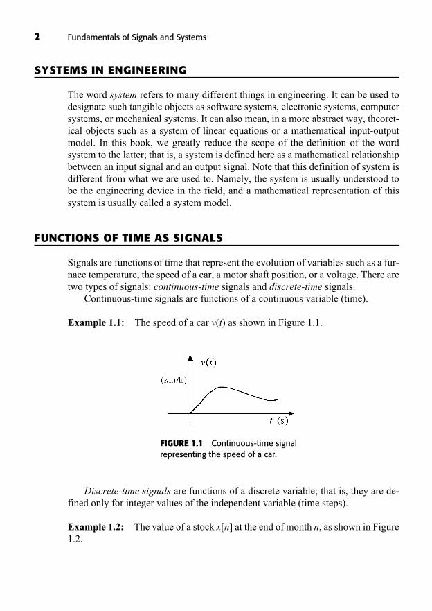
Example 1.1: The speed of a car v(t) as shown in Figure 1.1.
FIGURE 1.1 Continuous-time signalrepresenting the speed of a car.
Discrete-time signals are functions of a discrete variable; that is, they are de-fined only for integer values of the independent variable (time steps).
Example 1.2: The value of a stock x[n] at the end of month n, as shown in Figure1.2.
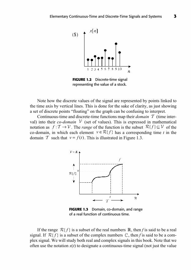
Note how the discrete values of the signal are represented by points linked tothe time axis by vertical lines. This is done for the sake of clarity, as just showinga set of discrete points “floating” on the graph can be confusing to interpret.
Continuous-time and discrete-time functions map their domain (time inter-val) into their co-domain (set of values). This is expressed in mathematicalnotation as . The range of the function is the subset of theco-domain, in which each element has a corresponding time t in thedomain such that . This is illustrated in Figure 1.3.v f t= ( )T
v fR{ }R V{ }ff :T V
VT
Elementary Continuous-Time and Discrete-Time Signals and Systems 3
FIGURE 1.2 Discrete-time signalrepresenting the value of a stock.
FIGURE 1.3 Domain, co-domain, and rangeof a real function of continuous time.
If the range is a subset of the real numbers , then f is said to be a realsignal. If is a subset of the complex numbers , then f is said to be a com-plex signal. We will study both real and complex signals in this book. Note that weoften use the notation x(t) to designate a continuous-time signal (not just the value
CR{ }fRR{ }f

4 Fundamentals of Signals and Systems
of x at time t) and x[n] to designate a discrete-time signal (again for the whole sig-nal, not just the value of x at time n).
For the car speed example above, the domain of v(t) could be withunits of seconds, assuming the car keeps on running forever, and the range is
, the set of all non-negative speeds in units of kilometers per hour.For the stock trend example, the domain of x[n] is the set of positive natural num-
bers , the co-domain is the non-negative reals , andthe range could be in dollar unit.
An example of a complex signal is the complex exponential , forwhich , , and ; that is, the set of all complexnumbers of magnitude equal to one.
TRANSFORMATIONS OF THE TIME VARIABLE
Consider the continuous-time signal x(t) defined by its graph shown in Figure 1.4and the discrete-time signal x[n] defined by its graph in Figure 1.5. As an aside,these two signals are said to be of finite support, as they are nonzero only over afinite time interval, namely on for x(t) and when for x[n].We will use these two signals to illustrate some useful transformations of the timevariable, such as time scaling and time reversal.
n { , , }3 3…t [ , ]2 2
R{ } { : }x z z= =C 1V = CT = �x t e j t( ) = 10
R{ } [ , ]x = 0 100V = +[ , )0 RT ={ , , , }1 2 3…
V = +[ , )0 R
T = +[ , )0
FIGURE 1.4 Graph of continuoustime signal x(t).
FIGURE 1.5 Graph of discrete-timesignal x[n].
Time Scaling
Time scaling refers to the multiplication of the time variable by a real positive con-stant . In the continuous-time case, we can write
(1.1)y t x t( ) ( ).=
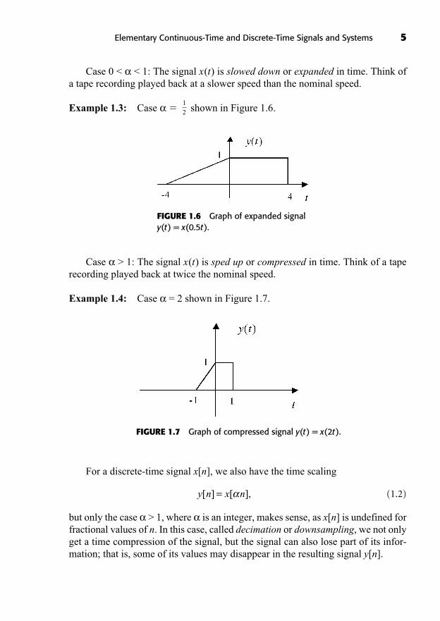
Case 0 < < 1: The signal x(t) is slowed down or expanded in time. Think ofa tape recording played back at a slower speed than the nominal speed.
Example 1.3: Case � shown in Figure 1.6.1
2
Elementary Continuous-Time and Discrete-Time Signals and Systems 5
FIGURE 1.6 Graph of expanded signaly(t) = x(0.5t).
Case > 1: The signal x(t) is sped up or compressed in time. Think of a taperecording played back at twice the nominal speed.
Example 1.4: Case = 2 shown in Figure 1.7.
FIGURE 1.7 Graph of compressed signal y(t) = x(2t).
For a discrete-time signal x[n], we also have the time scaling
(1.2)
but only the case > 1, where is an integer, makes sense, as x[n] is undefined forfractional values of n. In this case, called decimation or downsampling, we not onlyget a time compression of the signal, but the signal can also lose part of its infor-mation; that is, some of its values may disappear in the resulting signal y[n].
y n x n[ ] [ ],=
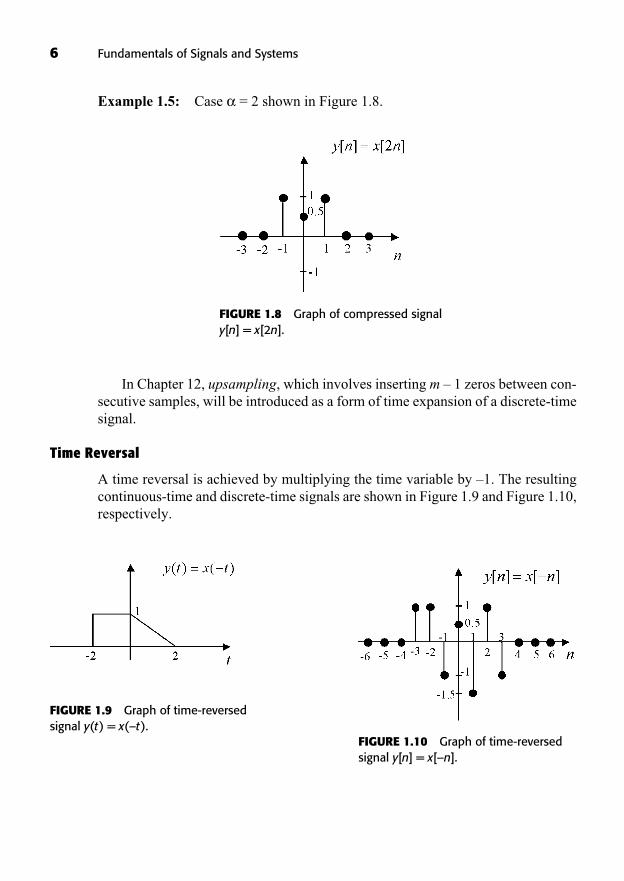
Example 1.5: Case = 2 shown in Figure 1.8.
6 Fundamentals of Signals and Systems
FIGURE 1.8 Graph of compressed signaly[n] = x[2n].
In Chapter 12, upsampling, which involves inserting m – 1 zeros between con-secutive samples, will be introduced as a form of time expansion of a discrete-timesignal.
Time Reversal
A time reversal is achieved by multiplying the time variable by –1. The resultingcontinuous-time and discrete-time signals are shown in Figure 1.9 and Figure 1.10,respectively.
FIGURE 1.9 Graph of time-reversedsignal y(t) = x(–t).
FIGURE 1.10 Graph of time-reversedsignal y[n] = x[–n].
Time Shift
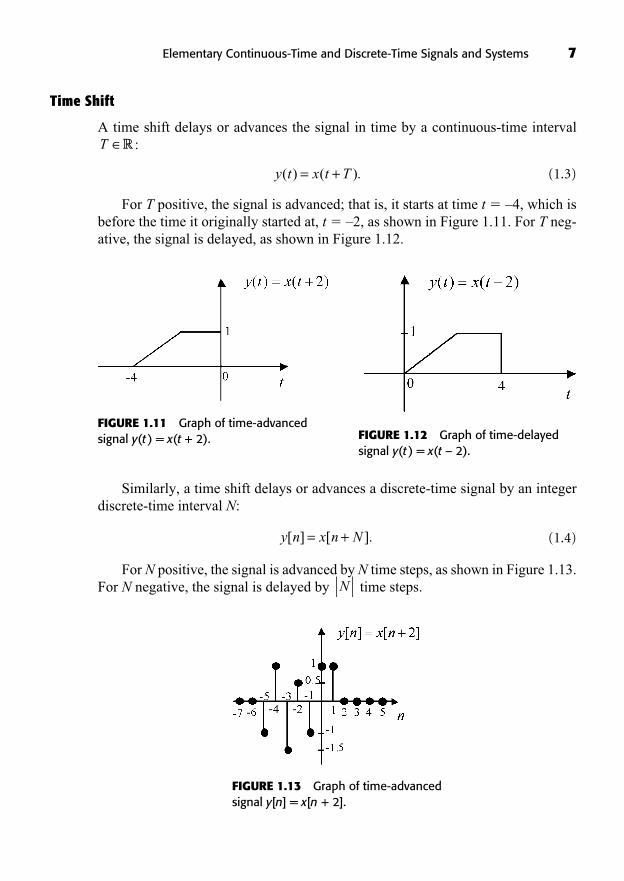
A time shift delays or advances the signal in time by a continuous-time interval:
(1.3)
For T positive, the signal is advanced; that is, it starts at time t � –4, which isbefore the time it originally started at, t � –2, as shown in Figure 1.11. For T neg-ative, the signal is delayed, as shown in Figure 1.12.
y t x t T( ) ( ).= +
T R
Elementary Continuous-Time and Discrete-Time Signals and Systems 7
FIGURE 1.11 Graph of time-advancedsignal y(t ) = x(t + 2). FIGURE 1.12 Graph of time-delayed
signal y(t ) = x(t – 2).
Similarly, a time shift delays or advances a discrete-time signal by an integerdiscrete-time interval N:
(1.4)
For N positive, the signal is advanced by N time steps, as shown in Figure 1.13.For N negative, the signal is delayed by time steps.N
y n x n N[ ] [ ].= +
FIGURE 1.13 Graph of time-advancedsignal y[n] = x[n + 2].
8 Fundamentals of Signals and Systems
PERIODIC SIGNALS
Intuitively, a signal is periodic when it repeats itself. This intuition is captured inthe following definition: a continuous-time signal x(t) is periodic if there exists apositive real T for which
(1.5)
A discrete-time signal x[n] is periodic if there exists a positive integer N forwhich
(1.6)
The smallest such T or N is called the fundamental period of the signal.
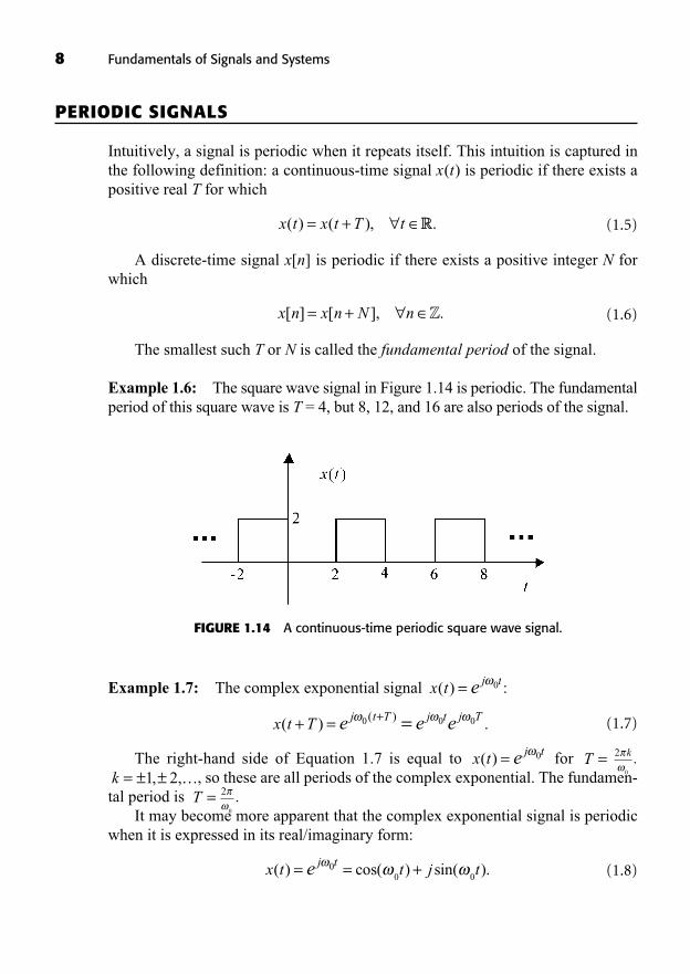
Example 1.6: The square wave signal in Figure 1.14 is periodic. The fundamentalperiod of this square wave is T = 4, but 8, 12, and 16 are also periods of the signal.
x n x n N n[ ] [ ], .= + Z
x t x t T t( ) ( ), .= + R
FIGURE 1.14 A continuous-time periodic square wave signal.
Example 1.7: The complex exponential signal :
(1.7)
The right-hand side of Equation 1.7 is equal to for , so these are all periods of the complex exponential. The fundamen-
tal period is .It may become more apparent that the complex exponential signal is periodic
when it is expressed in its real/imaginary form:
(1.8)x t t j te j t( ) cos( ) sin( ).= = +00 0
2
0
T =k = ± ±1 2, ,…
k2
0
,T =x t e j t( ) = 0
x t T e e ej t T j t j T( ) .( )+ = + =0 0 0
x t e j t( ) = 0
where it is clear that the real part, , and the imaginary part, , areperiodic with fundamental period .
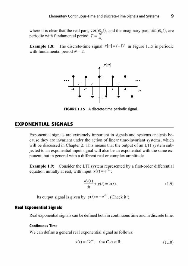
Example 1.8: The discrete-time signal in Figure 1.15 is periodicwith fundamental period N = 2.
x n n[ ] ( )= 1
2
0
T =sin( )
0tcos( )
0t
Elementary Continuous-Time and Discrete-Time Signals and Systems 9
FIGURE 1.15 A discrete-time periodic signal.
EXPONENTIAL SIGNALS
Exponential signals are extremely important in signals and systems analysis be-cause they are invariant under the action of linear time-invariant systems, whichwill be discussed in Chapter 2. This means that the output of an LTI system sub-jected to an exponential input signal will also be an exponential with the same ex-ponent, but in general with a different real or complex amplitude.
Example 1.9: Consider the LTI system represented by a first-order differentialequation initially at rest, with input :
(1.9)
Its output signal is given by . (Check it!)
Real Exponential Signals
Real exponential signals can be defined both in continuous time and in discrete time.
Continuous Time
We can define a general real exponential signal as follows:
(1.10)x t Ce Ct( ) , , .= 0 R
y t e t( ) = 2
dy t
dty t x t
( )( ) ( ).+ =
x t e t( ) = 2
10 Fundamentals of Signals and Systems
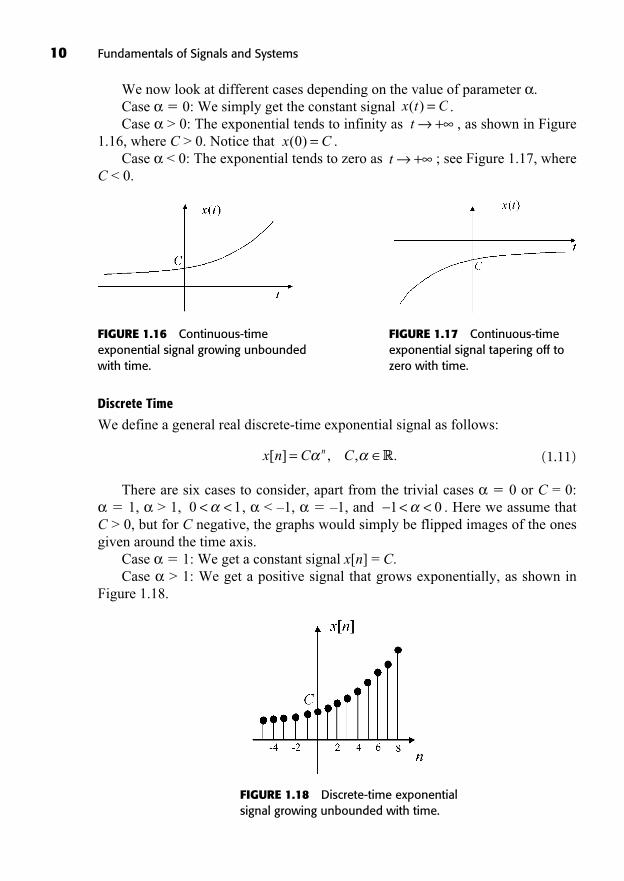
We now look at different cases depending on the value of parameter .Case � 0: We simply get the constant signal .Case > 0: The exponential tends to infinity as , as shown in Figure
1.16, where C > 0. Notice that .Case < 0: The exponential tends to zero as ; see Figure 1.17, where
C < 0.t +
x C( )0 =t +
x t C( ) =
FIGURE 1.16 Continuous-timeexponential signal growing unboundedwith time.
FIGURE 1.17 Continuous-timeexponential signal tapering off tozero with time.
Discrete Time
We define a general real discrete-time exponential signal as follows:
(1.11)
There are six cases to consider, apart from the trivial cases � 0 or C = 0: � 1, > 1, , < –1, � –1, and . Here we assume that
C > 0, but for C negative, the graphs would simply be flipped images of the onesgiven around the time axis.
Case � 1: We get a constant signal x[n] = C.Case > 1: We get a positive signal that grows exponentially, as shown in
Figure 1.18.
< <1 00 1< <
x n C Cn[ ] , , .= R
FIGURE 1.18 Discrete-time exponentialsignal growing unbounded with time.
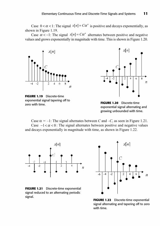
Case : The signal is positive and decays exponentially, asshown in Figure 1.19.
Case : The signal alternates between positive and negativevalues and grows exponentially in magnitude with time. This is shown in Figure 1.20.
x n C n[ ] =< 1
x n C n[ ] =0 1< <
Elementary Continuous-Time and Discrete-Time Signals and Systems 11
FIGURE 1.19 Discrete-timeexponential signal tapering off tozero with time. FIGURE 1.20 Discrete-time
exponential signal alternating andgrowing unbounded with time.
FIGURE 1.21 Discrete-time exponentialsignal reduced to an alternating periodicsignal.
FIGURE 1.22 Discrete-time exponentialsignal alternating and tapering off to zerowith time.
Case � –1: The signal alternates between C and –C, as seen in Figure 1.21.Case : The signal alternates between positive and negative values
and decays exponentially in magnitude with time, as shown in Figure 1.22.< <1 0
((Lecture 2: Some Useful Signals))
Complex Exponential Signals
Complex exponential signals can also be defined both in continuous time and indiscrete time. They have real and imaginary parts with sinusoidal behavior.
Continuous Time
The continuous-time complex exponential signal can be defined as follows:
(1.12)
where is expressed in polar form, and is expressed in rectangular form. Thus, we can write
(1.13)
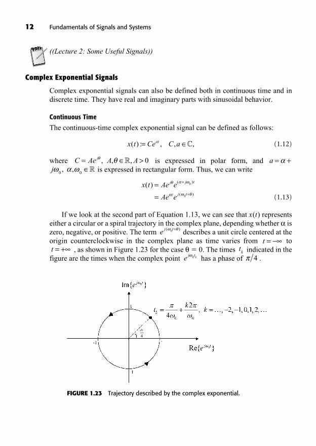
If we look at the second part of Equation 1.13, we can see that x(t) representseither a circular or a spiral trajectory in the complex plane, depending whether iszero, negative, or positive. The term describes a unit circle centered at theorigin counterclockwise in the complex plane as time varies from to
, as shown in Figure 1.23 for the case � 0. The times indicated in thefigure are the times when the complex point has a phase of .4e j tk0
tkt = +
t =e j t( )0 +
x t Ae e
Ae e
j j t
t j t
( ) ( )
( )
=
=
+
+
0
0
j0 0, , �
a = +C Ae A Aj= >, , ,� 0
x t Ce C aat( ) : , , ,= C
12 Fundamentals of Signals and Systems
FIGURE 1.23 Trajectory described by the complex exponential.
Using Euler’s relation, we obtain the signal in rectangular form:
(1.14)
where and are the realpart and imaginary part of the signal, respectively. Both are sinusoidal, with time-varying amplitude (or envelope) . We can see that the exponent defines the type of real and imaginary parts we get for the signal.
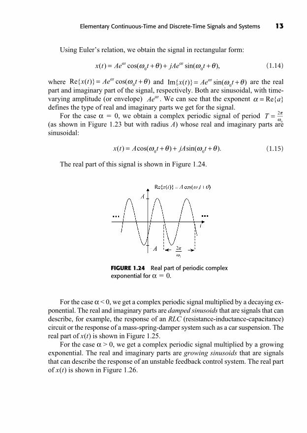
For the case � 0, we obtain a complex periodic signal of period (as shown in Figure 1.23 but with radius A) whose real and imaginary parts are sinusoidal:
(1.15)
The real part of this signal is shown in Figure 1.24.
x t A t jA t( ) cos( ) sin( ).= + + +0 0
2
0
T =
= Re{ }aAe t
Im{ ( )} sin( )x t Ae tt= +0
Re{ ( )} cos( )x t Ae tt= +0
x t Ae t jAe tt t( ) cos( ) sin( ),= + + +0 0
Elementary Continuous-Time and Discrete-Time Signals and Systems 13
FIGURE 1.24 Real part of periodic complexexponential for � 0.
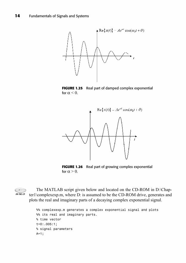
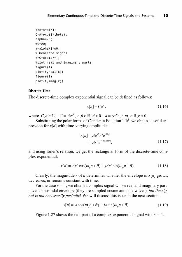
For the case < 0, we get a complex periodic signal multiplied by a decaying ex-ponential. The real and imaginary parts are damped sinusoids that are signals that candescribe, for example, the response of an RLC (resistance-inductance-capacitance)circuit or the response of a mass-spring-damper system such as a car suspension. Thereal part of x(t) is shown in Figure 1.25.
For the case > 0, we get a complex periodic signal multiplied by a growingexponential. The real and imaginary parts are growing sinusoids that are signalsthat can describe the response of an unstable feedback control system. The real partof x(t) is shown in Figure 1.26.
14 Fundamentals of Signals and Systems
The MATLAB script given below and located on the CD-ROM in D:\Chap-ter1\complexexp.m, where D: is assumed to be the CD-ROM drive, generates andplots the real and imaginary parts of a decaying complex exponential signal.
%% complexexp.m generates a complex exponential signal and plots
%% its real and imaginary parts.
% time vector
t=0:.005:1;
% signal parameters
A=1;
FIGURE 1.25 Real part of damped complex exponentialfor < 0.
FIGURE 1.26 Real part of growing complex exponentialfor > 0.
theta=pi/4;
C=A*exp(j*theta);
alpha=-3;
w0=20;
a=alpha+j*w0;
% Generate signal
x=C*exp(a*t);
%plot real and imaginary parts
figure(1)
plot(t,real(x))
figure(2)
plot(t,imag(x))
Discrete Time
The discrete-time complex exponential signal can be defined as follows:
(1.16)
where .Substituting the polar forms of C and a in Equation 1.16, we obtain a useful ex-
pression for x[n] with time-varying amplitude:
(1.17)
and using Euler’s relation, we get the rectangular form of the discrete-time com-plex exponential:
(1.18)
Clearly, the magnitude r of a determines whether the envelope of x[n] grows,decreases, or remains constant with time.
For the case r � 1, we obtain a complex signal whose real and imaginary partshave a sinusoidal envelope (they are sampled cosine and sine waves), but the sig-nal is not necessarily periodic! We will discuss this issue in the next section.
(1.19)
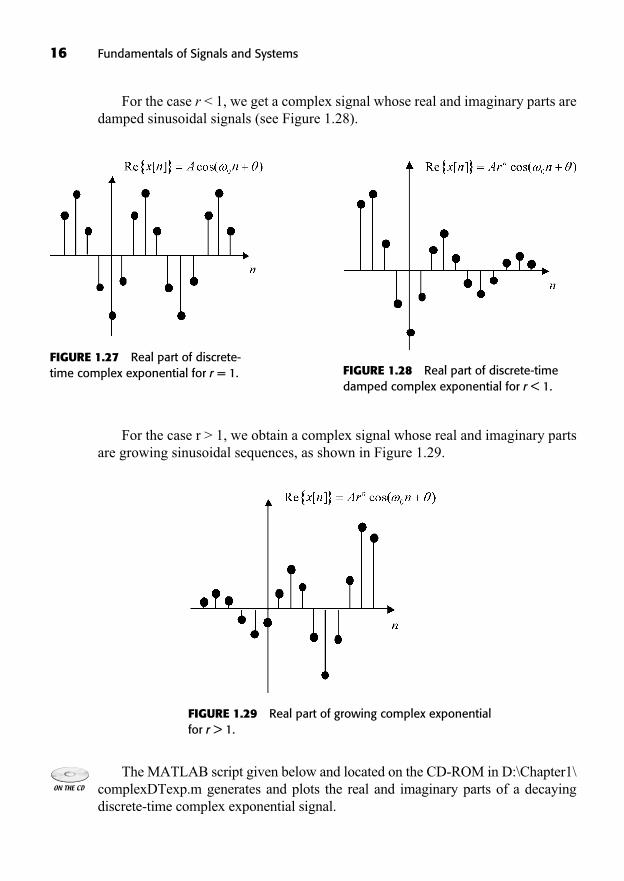
Figure 1.27 shows the real part of a complex exponential signal with r � 1.
x n A n jA n[ ] cos( ) sin( )= + + +0 0
x n Ar n jAr nn n[ ] cos( ) sin( ).= + + +0 0
x n Ae r e
Ar e
j n j n
n j n
[ ]
,( )
=
= +
0
0
C a C Ae A A a re r rj j, , , , , , ,= > = >C, � �0 00
0
x n Can[ ] ,=
Elementary Continuous-Time and Discrete-Time Signals and Systems 15
16 Fundamentals of Signals and Systems
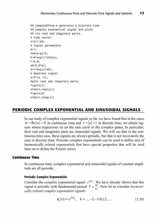
For the case r < 1, we get a complex signal whose real and imaginary parts aredamped sinusoidal signals (see Figure 1.28).
FIGURE 1.27 Real part of discrete-time complex exponential for r = 1. FIGURE 1.28 Real part of discrete-time
damped complex exponential for r < 1.
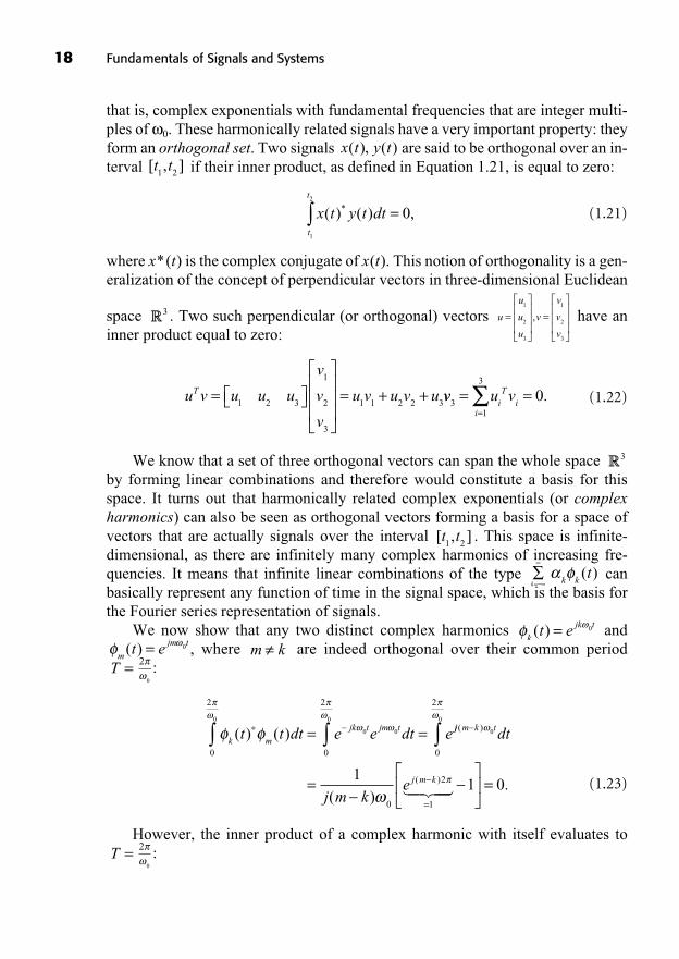
For the case r > 1, we obtain a complex signal whose real and imaginary partsare growing sinusoidal sequences, as shown in Figure 1.29.
FIGURE 1.29 Real part of growing complex exponentialfor r > 1.
The MATLAB script given below and located on the CD-ROM in D:\Chapter1\complexDTexp.m generates and plots the real and imaginary parts of a decayingdiscrete-time complex exponential signal.
%% complexDTexp.m generates a discrete-time
%% complex exponential signal and plots
%% its real and imaginary parts.
% time vector
n=0:1:20;
% signal parameters
A=1;
theta=pi/4;
C=A*exp(j*theta);
r=0.8;
w0=0.2*pi;
a=r*exp(j*w0);
% Generate signal
x=C*(a.^n);
%plot real and imaginary parts
figure(1)
stem(n,real(x))
figure(2)
stem(n,imag(x))
PERIODIC COMPLEX EXPONENTIAL AND SINUSOIDAL SIGNALS
In our study of complex exponential signals so far, we have found that in the casesin continuous time and in discrete time, we obtain sig-
nals whose trajectories lie on the unit circle in the complex plane. In particular,their real and imaginary parts are sinusoidal signals. We will see that in the con-tinuous-time case, these signals are always periodic, but that is not necessarily thecase in discrete time. Periodic complex exponentials can be used to define sets ofharmonically related exponentials that have special properties that will be usedlater on to define the Fourier series.
Continuous Time
In continuous time, complex exponential and sinusoidal signals of constant ampli-tude are all periodic.
Periodic Complex Exponentials
Consider the complex exponential signal . We have already shown that thissignal is periodic with fundamental period . Now let us consider harmoni-cally related complex exponential signals:
(1.20)k
jk tt e k( ) : , , , , , , , ,= =0 2 1 0 1 2… …
2
0
T =e j t0
r a= = 1= =Re{ }a 0
Elementary Continuous-Time and Discrete-Time Signals and Systems 17
that is, complex exponentials with fundamental frequencies that are integer multi-ples of 0. These harmonically related signals have a very important property: theyform an orthogonal set. Two signals are said to be orthogonal over an in-terval if their inner product, as defined in Equation 1.21, is equal to zero:
(1.21)
where x*(t) is the complex conjugate of x(t). This notion of orthogonality is a gen-eralization of the concept of perpendicular vectors in three-dimensional Euclidean
space . Two such perpendicular (or orthogonal) vectors have aninner product equal to zero:
(1.22)
We know that a set of three orthogonal vectors can span the whole space by forming linear combinations and therefore would constitute a basis for thisspace. It turns out that harmonically related complex exponentials (or complexharmonics) can also be seen as orthogonal vectors forming a basis for a space ofvectors that are actually signals over the interval . This space is infinite-dimensional, as there are infinitely many complex harmonics of increasing fre-quencies. It means that infinite linear combinations of the type canbasically represent any function of time in the signal space, which is the basis forthe Fourier series representation of signals.
We now show that any two distinct complex harmonics and, where are indeed orthogonal over their common period
:
(1.23)
However, the inner product of a complex harmonic with itself evaluates to:2
0
T =
k m
jk t jm tt t dt e e dt e( ) ( ) = =0
2
0
2
0
0 0
0jj m k t
j m k
dt
j m ke
( )
( )
( ) =
=
0
0
0
2
0
2
1
1��� ��� =1 0.
2
0
T =m km
jm tt e( ) = 0k
jk tt e( ) = 0
k kt( )
k=
[ , ]t t1 2
R3
u v u u u
v
v
v
u v u v uT = = + +1 2 3
1
2
3
1 1 2 2 3vv u v
iT
ii
31
3
0= ==
.
u
u
u
u
v
v
v
v
= =1
2
3
1
2
3
,R3
x t y t dtt
t
( ) ( ) ,*
1
2
0=
[ , ]t t1 2
x t y t( ), ( )
18 Fundamentals of Signals and Systems
Elementary Continuous-Time and Discrete-Time Signals and Systems 19
(1.24)
Sinusoidal Signals
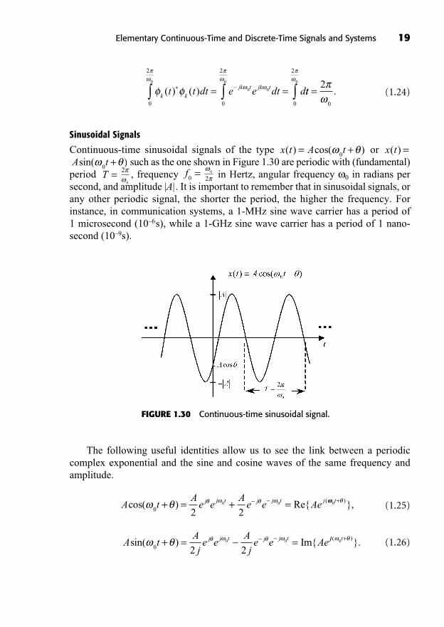
Continuous-time sinusoidal signals of the type or such as the one shown in Figure 1.30 are periodic with (fundamental)
period , frequency in Hertz, angular frequency 0 in radians persecond, and amplitude |A|. It is important to remember that in sinusoidal signals, orany other periodic signal, the shorter the period, the higher the frequency. Forinstance, in communication systems, a 1-MHz sine wave carrier has a period of 1 microsecond (10–6s), while a 1-GHz sine wave carrier has a period of 1 nano-second (10–9s).
0
2f
0=2
0
T =A tsin( )+
0
x t( ) =x t A t( ) cos( )= +0
k k
jk t jk tt t dt e e dt d( ) ( ) = =0
2
0
2
0
0 0
0
tt0
2
0
0 2= .
FIGURE 1.30 Continuous-time sinusoidal signal.
The following useful identities allow us to see the link between a periodiccomplex exponential and the sine and cosine waves of the same frequency andamplitude.
(1.25)
(1.26)A tA
je e
A
je e Aej j t j j tsin( ) Im{
0 2 20 0+ = = jj t( )}.0 +
A tA
e eA
e e Aej j t j j t jcos( ) Re{ (
0 2 20 0+ = + = 0t+ )},
Discrete Time
In discrete time, complex exponential and sinusoidal signals of constant amplitudeare not necessarily periodic.
Complex Exponential Signals
The complex exponential signal is not periodic in general, although it seemslike it is for any 0. The intuitive explanation is that the signal values, which arepoints on the unit circle in the complex plane, do not necessarily fall at the samelocations as time evolves and the circle is described counterclockwise. When thesignal values do always fall on the same points, then the discrete-time complexexponential is periodic. A more detailed analysis of periodicity is left for the nextsubsection on discrete-time sinusoidal signals, but it also applies to complex expo-nential signals.
The discrete-time complex harmonic signals defined by
(1.27)
are periodic of (not necessarily fundamental) period N. They are also orthogonal,with the integral replaced by a sum in the inner product:
(1.28)
Here there are only N such distinct complex harmonics. For example, for N =8, we could easily check that . These signals will be used in Chap-ter 12 to define the discrete-time Fourier series.
Sinusoidal Signals
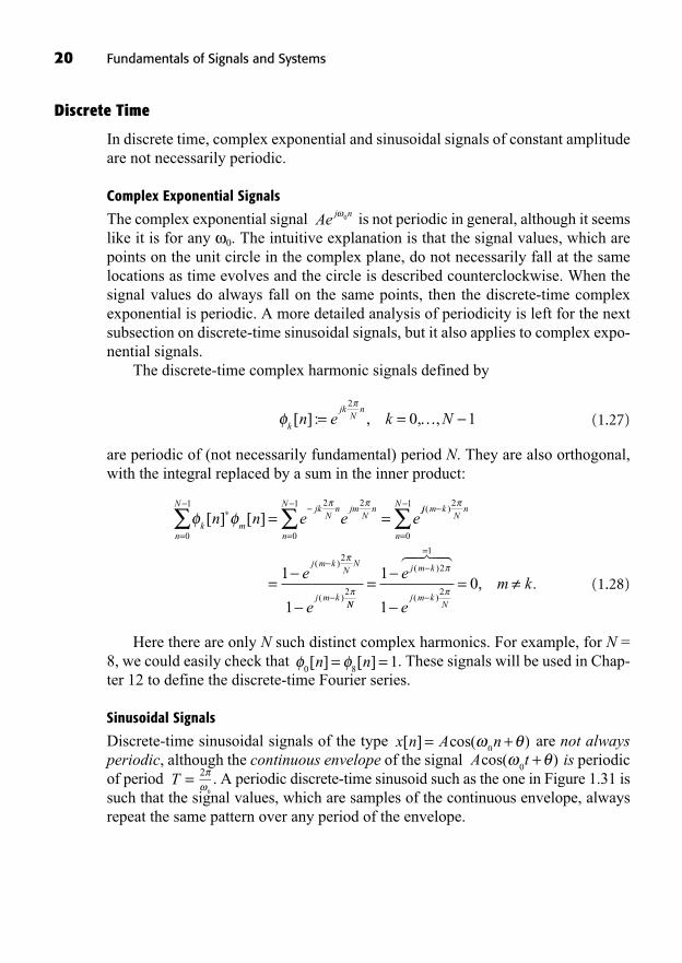
Discrete-time sinusoidal signals of the type are not alwaysperiodic, although the continuous envelope of the signal is periodicof period . A periodic discrete-time sinusoid such as the one in Figure 1.31 issuch that the signal values, which are samples of the continuous envelope, alwaysrepeat the same pattern over any period of the envelope.
2
0
T =A tcos( )
0+
x n A n[ ] cos( )= +0
0 81[ ] [ ]n n= =
k mn
Njk
Nn jm
Nn
n
N
n n e e e[ ] [ ]= =
= =0
1 2 2
0
1jj m k
Nn
n
N
j m kN
N
j m k
e
e
( )
( )
( )
=
=
2
0
1
2
2
1
1 NN
j m k
j m kN
e
e
m k= =
=
1
1
02
1
2
( )
( ), .
��� �
k
jkN
nn e k N[ ] : , , ,= =
2
0 1…
Ae j n0
20 Fundamentals of Signals and Systems
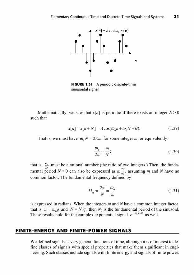
Elementary Continuous-Time and Discrete-Time Signals and Systems 21
Mathematically, we saw that x[n] is periodic if there exists an integer N > 0such that
(1.29)
That is, we must have for some integer m, or equivalently:
(1.30)
that is, must be a rational number (the ratio of two integers.) Then, the funda-mental period N > 0 can also be expressed as m , assuming m and N have no common factor. The fundamental frequency defined by
(1.31)
is expressed in radians. When the integers m and N have a common integer factor,that is, and , then N0 is the fundamental period of the sinusoid.These results hold for the complex exponential signal as well.
FINITE-ENERGY AND FINITE-POWER SIGNALS
We defined signals as very general functions of time, although it is of interest to de-fine classes of signals with special properties that make them significant in engi-neering. Such classes include signals with finite energy and signals of finite power.
e j n( )0 +N N q=
0m m q=0
002
:= =N m
2
0
0
2
0
2=
m
N;
02N m=
x n x n N A n N[ ] [ ] cos( ).= + = + +0 0
FIGURE 1.31 A periodic discrete-timesinusoidal signal.

The instantaneous power dissipated in a resistor of resistance R is simply theproduct of the voltage across and the current through the resistor:
(1.32)
and the total energy dissipated during a time interval is obtained by inte-grating the power
(1.33)
The average power dissipated over that interval is the total energy divided bythe time interval:
(1.34)
Analogously, the total energy and average power over of an arbitrary integrable continuous-time signal x(t) are defined as though the signal were a volt-age across a one-ohm resistor:
(1.35)
(1.36)
The total energy and total average power of a signal defined over are de-fined as
(1.37)
(1.38)
The total energy and average power over of an arbitrary discrete-timesignal x[n] are defined as
(1.39)E x nn n n n
n
[ , ]: | [ ] | ,
1 2 1
2 2==
[ , ]n n1 2
PT
x t dtT T
T=: lim | ( ) | .
1
22
E x t dt x t dtT T
T= =: lim | ( ) | | ( ) | ,2 2
t R
Pt t
x t dtt t t
t
[ , ]: | ( ) | .
1 2 1
21
2 1
2=
E x t dtt t t
t
[ , ]: | ( ) | ,
1 2 1
2 2=
[ , ]t t1 2
Pt t
v t
Rdt
t t t
t
[ , ]
( ).
1 2 1
21
2 1
2
=
E p t dtv t
Rdt
t t t
t
t
t
[ , ]( )
( ).
1 2 1
2
1
22
= =
[ , ]t t1 2
p t v t i tv t
R( ) ( ) ( )
( ),= =
2
22 Fundamentals of Signals and Systems
(1.40)
Notice that is the number of points in the signal over the interval. The total energy and total average power of signal x[n] defined over
are defined as
(1.41)
(1.42)
The class of continuous-time or discrete-time finite-energy signals is definedas the set of all signals for which .
Example 1.10: The discrete-time signal , for whichis a finite-energy signal.
The class of continuous-time or discrete-time finite-power signals is defined asthe set of all signals for which .
Example 1.11: The constant signal has infinite energy, but a total aver-age power of 16:
(1.43)
The total average power of a periodic signal can be calculated over one periodonly as .
Example 1.12: For , the total average power is computed as
(1.44)
Note that has unit power.
EVEN AND ODD SIGNALS
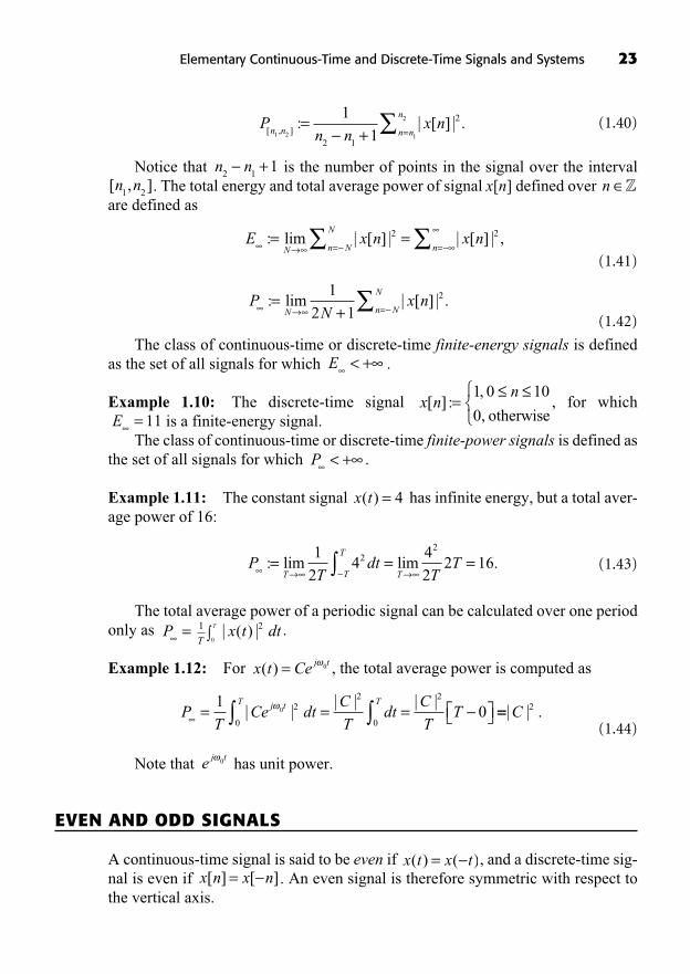
A continuous-time signal is said to be even if , and a discrete-time sig-nal is even if . An even signal is therefore symmetric with respect tothe vertical axis.
x n x n[ ] [ ]=x t x t( ) ( )=
e j t0
PT
Ce dtC
Tdt
C
TTj tT T
= = =1
00 2
0
2
0
2
| || | | |
==| | .C 2
x t Ce j t( ) = 0
x t dtT
2| ( ) |T
T10
P =
PT
dtT
TT T
T
T= = =: lim lim .
1
24
4
22 162
2
x t( ) = 4
P < +
E = 11x n
n[ ] :
,
,=
1 0 10
0 otherwise
E < +
PN
x nN n N
N
==
+: lim | [ ] | .
1
2 12
E x n x nN n N
N
n= == =: lim | [ ] | | [ ] | ,2 2
n Z[ , ]n n1 2
n n2 1
1+
Pn n
x nn n n n
n
[ , ]: | [ ] | .
1 2 1
21
12 1
2=+ =
Elementary Continuous-Time and Discrete-Time Signals and Systems 23
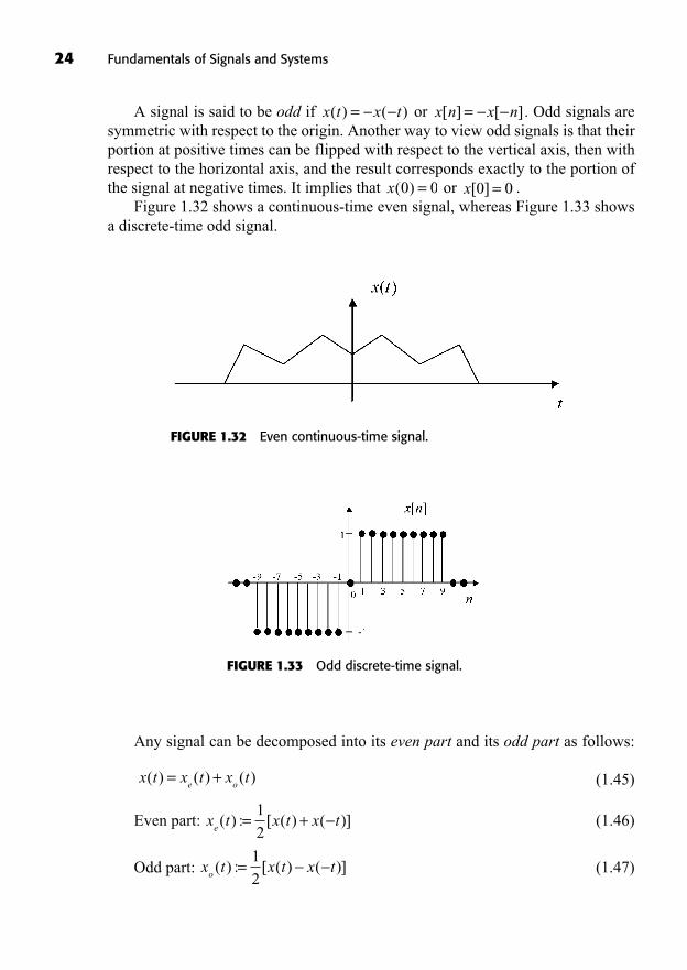
A signal is said to be odd if or . Odd signals aresymmetric with respect to the origin. Another way to view odd signals is that theirportion at positive times can be flipped with respect to the vertical axis, then withrespect to the horizontal axis, and the result corresponds exactly to the portion ofthe signal at negative times. It implies that or .
Figure 1.32 shows a continuous-time even signal, whereas Figure 1.33 showsa discrete-time odd signal.
x[ ]0 0=x( )0 0=
x n x n[ ] [ ]=x t x t( ) ( )=
24 Fundamentals of Signals and Systems
FIGURE 1.32 Even continuous-time signal.
FIGURE 1.33 Odd discrete-time signal.
Any signal can be decomposed into its even part and its odd part as follows:
(1.45)
Even part: (1.46)
Odd part: (1.47)x t x t x to( ) : [ ( ) ( )]=
1
2
x t x t x te( ) : [ ( ) ( )]= +
1
2
x t x t x te o
( ) ( ) ( )= +
The even part and odd parts of a discrete-time signal are defined in the exactsame way.
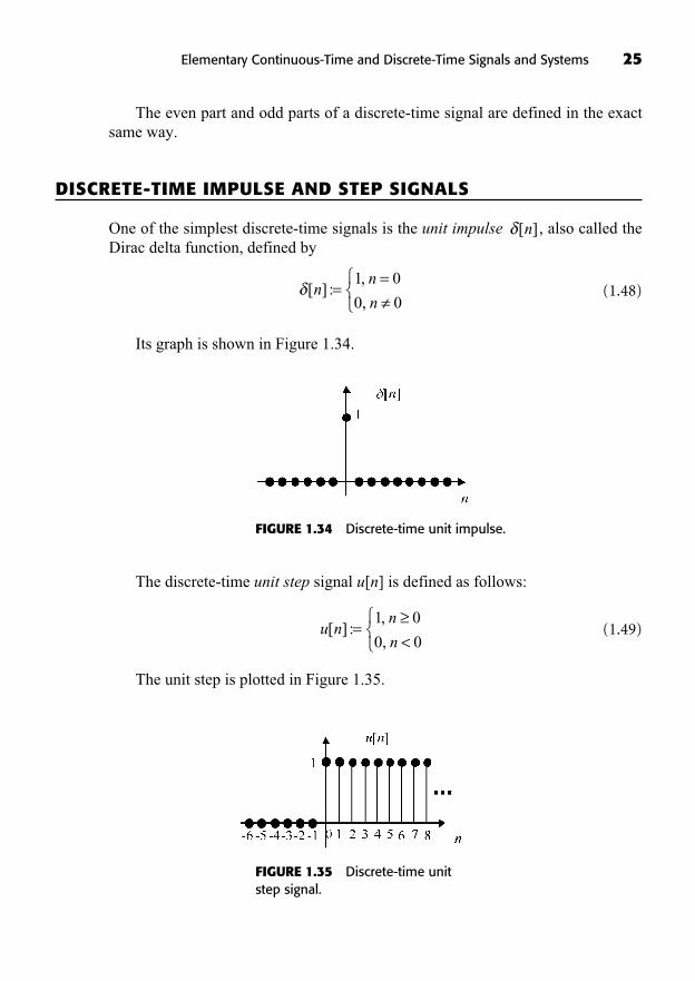
DISCRETE-TIME IMPULSE AND STEP SIGNALS
One of the simplest discrete-time signals is the unit impulse , also called theDirac delta function, defined by
(1.48)
Its graph is shown in Figure 1.34.
[ ] :,
,n
n
n=
=1 0
0 0
[ ]n
Elementary Continuous-Time and Discrete-Time Signals and Systems 25
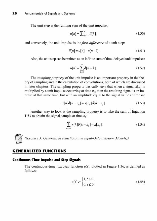
FIGURE 1.34 Discrete-time unit impulse.
The discrete-time unit step signal u[n] is defined as follows:
(1.49)
The unit step is plotted in Figure 1.35.
u nn
n[ ] :
,
,=
<1 0
0 0
FIGURE 1.35 Discrete-time unitstep signal.
26 Fundamentals of Signals and Systems
The unit step is the running sum of the unit impulse:
(1.50)
and conversely, the unit impulse is the first-difference of a unit step:
(1.51)
Also, the unit step can be written as an infinite sum of time-delayed unit impulses:
(1.52)
The sampling property of the unit impulse is an important property in the the-ory of sampling and in the calculation of convolutions, both of which are discussedin later chapters. The sampling property basically says that when a signal x[n] ismultiplied by a unit impulse occurring at time n0, then the resulting signal is an im-pulse at that same time, but with an amplitude equal to the signal value at time n0:
(1.53)
Another way to look at the sampling property is to take the sum of Equation1.53 to obtain the signal sample at time n0:
(1.54)
((Lecture 3: Generalized Functions and Input-Output System Models))
GENERALIZED FUNCTIONS
Continuous-Time Impulse and Step Signals
The continuous-time unit step function u(t), plotted in Figure 1.36, is defined asfollows:
(1.55)u tt
t( ) :
,
,=
>1 0
0 0
x k k n x nk
[ ] [ ] [ ].==
+
0 0
x n n n x n n n[ ] [ ] [ ] [ ].=0 0 0
u n n kk
[ ] [ ].==0
[ ] [ ] [ ].n u n u n= 1
u n kk
n[ ] [ ],=
=
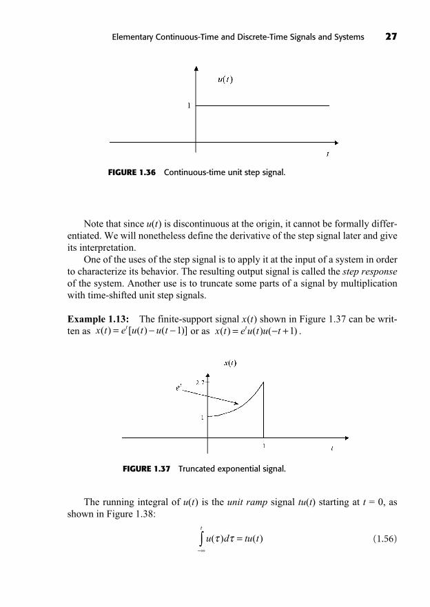
Note that since u(t) is discontinuous at the origin, it cannot be formally differ-entiated. We will nonetheless define the derivative of the step signal later and giveits interpretation.
One of the uses of the step signal is to apply it at the input of a system in orderto characterize its behavior. The resulting output signal is called the step responseof the system. Another use is to truncate some parts of a signal by multiplicationwith time-shifted unit step signals.
Example 1.13: The finite-support signal x(t) shown in Figure 1.37 can be writ-ten as or as .x t e u t u tt( ) ( ) ( )= +1x t e u t u tt( ) [ ( ) ( )]= 1
Elementary Continuous-Time and Discrete-Time Signals and Systems 27
FIGURE 1.36 Continuous-time unit step signal.
FIGURE 1.37 Truncated exponential signal.
The running integral of u(t) is the unit ramp signal tu(t) starting at t = 0, asshown in Figure 1.38:
(1.56)u d tu tt
( ) ( )=
28 Fundamentals of Signals and Systems
Successive integrals of u(t) yield signals with increasing powers of t :
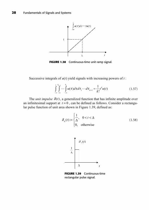
(1.57)
The unit impulse , a generalized function that has infinite amplitude overan infinitesimal support at , can be defined as follows. Consider a rectangu-lar pulse function of unit area shown in Figure 1.39, defined as:
(1.58)( ) :,
,
tt= < <
10
0 otherwise
t = 0( )t
u d d dk
t u tk
tk
k
( )!
( )1 1
11 1=
FIGURE 1.38 Continuous-time unit ramp signal.
FIGURE 1.39 Continuous-timerectangular pulse signal.
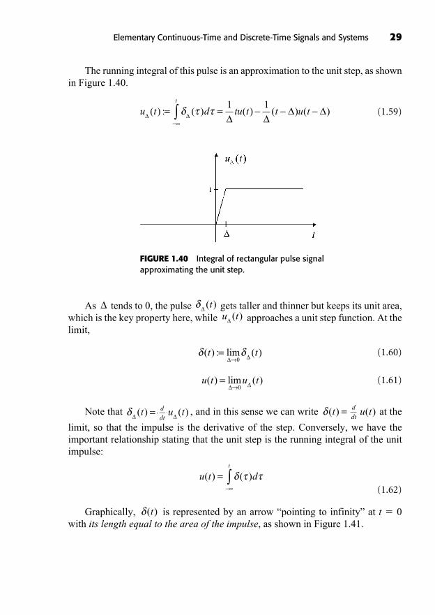
The running integral of this pulse is an approximation to the unit step, as shownin Figure 1.40.
(1.59)u t d tu t t u tt
( ) : ( ) ( ) ( ) ( )= =1 1
Elementary Continuous-Time and Discrete-Time Signals and Systems 29
FIGURE 1.40 Integral of rectangular pulse signalapproximating the unit step.
As tends to 0, the pulse gets taller and thinner but keeps its unit area,which is the key property here, while approaches a unit step function. At thelimit,
(1.60)
(1.61)
Note that , and in this sense we can write at the
limit, so that the impulse is the derivative of the step. Conversely, we have theimportant relationship stating that the unit step is the running integral of the unitimpulse:
(1.62)
Graphically, is represented by an arrow “pointing to infinity” at t � 0with its length equal to the area of the impulse, as shown in Figure 1.41.
( )t
u t dt
( ) ( )=
( )u td
dt( )t =( )u td
dt=( )t =
u t u t( ) lim ( )=0
( ) : lim ( )t t=0
u t( )( )t
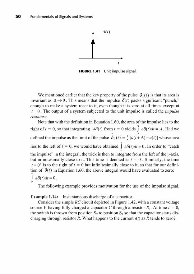
30 Fundamentals of Signals and Systems
We mentioned earlier that the key property of the pulse is that its area isinvariant as . This means that the impulse packs significant “punch,”enough to make a system react to it, even though it is zero at all times except at
. The output of a system subjected to the unit impulse is called the impulse response.
Note that with the definition in Equation 1.60, the area of the impulse lies to the
right of t � 0, so that integrating from t � 0 yields . Had we
defined the impulse as the limit of the pulse whose area
lies to the left of t � 0, we would have obtained . In order to “catch
the impulse” in the integral, the trick is then to integrate from the left of the y-axis,but infinitesimally close to it. This time is denoted as t � 0–. Similarly, the time
is to the right of t � 0 but infinitesimally close to it, so that for our defini-tion of in Equation 1.60, the above integral would have evaluated to zero:
.
The following example provides motivation for the use of the impulse signal.
Example 1.14: Instantaneous discharge of a capacitor.Consider the simple RC circuit depicted in Figure 1.42, with a constant voltage
source V having fully charged a capacitor C through a resistor R1. At time t � 0,the switch is thrown from position S2 to position S1 so that the capacitor starts dis-charging through resistor R. What happens to the current i(t) as R tends to zero?
A t dt( ) 0=0+
( )tt = +0
A t dt( ) 0=0
[ ( ) ( )]u t u t+1~
( ) :t =
A t dt A( ) =0
A t( )
t = 0
( )t0( )t
FIGURE 1.41 Unit impulse signal.
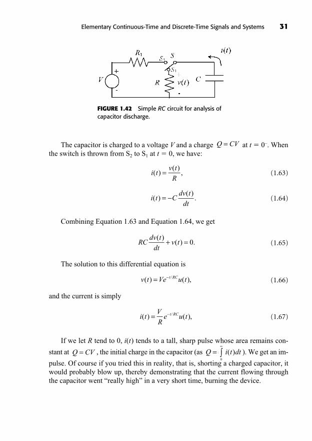
The capacitor is charged to a voltage V and a charge at t � 0–. Whenthe switch is thrown from S2 to S1 at t � 0, we have:
(1.63)
(1.64)
Combining Equation 1.63 and Equation 1.64, we get
(1.65)
The solution to this differential equation is
(1.66)
and the current is simply
(1.67)
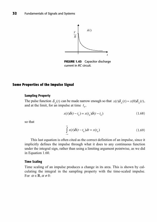
If we let R tend to 0, i(t) tends to a tall, sharp pulse whose area remains con-
stant at , the initial charge in the capacitor (as ). We get an im-
pulse. Of course if you tried this in reality, that is, shorting a charged capacitor, itwould probably blow up, thereby demonstrating that the current flowing throughthe capacitor went “really high” in a very short time, burning the device.
i t dt( )=0
Q =Q CV=
i tV
Re u tt RC( ) ( ),/=
v t Ve u tt RC( ) ( ),/=
RCdv t
dtv t
( )( ) .+ = 0
i t Cdv t
dt( )
( ).=
i tv t
R( )
( ),=
Q CV=
Elementary Continuous-Time and Discrete-Time Signals and Systems 31
FIGURE 1.42 Simple RC circuit for analysis ofcapacitor discharge.
Some Properties of the Impulse Signal
Sampling Property
The pulse function can be made narrow enough so that ,and at the limit, for an impulse at time ,
(1.68)
so that
(1.69)
This last equation is often cited as the correct definition of an impulse, since itimplicitly defines the impulse through what it does to any continuous functionunder the integral sign, rather than using a limiting argument pointwise, as we didin Equation 1.60.
Time Scaling
Time scaling of an impulse produces a change in its area. This is shown by cal-culating the integral in the sampling property with the time-scaled impulse. For :R, 0
x t t t dt x t( ) ( ) ( )=0 0
x t t t x t t t( ) ( ) ( ) ( )=0 0 0
t0
x t t x t( ) ( ) ( ) ( )0( )t
32 Fundamentals of Signals and Systems
FIGURE 1.43 Capacitor dischargecurrent in RC circuit.
(1.70)
Hence,
(1.71)
Note that the equality sign in Equation 1.71 means that both of these impulseshave the same effect under the integral in the sampling property.
Time Shift
The convolution of signals x(t) and y(t) is defined as
(1.72)
The convolution of signal x(t) with the time-delayed impulse delaysthe signal by T:
(1.73)
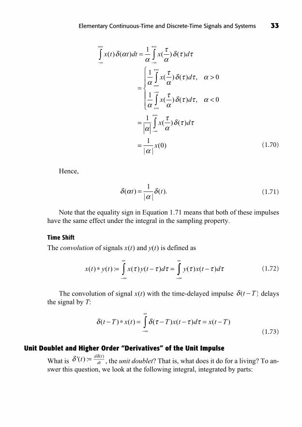
Unit Doublet and Higher Order “Derivatives” of the Unit Impulse
What is , the unit doublet? That is, what does it do for a living? To an-swer this question, we look at the following integral, integrated by parts:
( )d t
dt'( ) :t =
( ) ( ) ( ) ( ) ( )t T x t T x t d x t T= =
( )t T
x t y t x y t d y x t d( ) ( ) : ( ) ( ) ( ) ( )= =
( )| |
( ).t t=1
x t t dt x d
x
( ) ( ) ( ) ( )
( )
+ +
=
=
1
1 +
+
>
<
( ) ,
( ) ( ) ,
d
x d
0
10
=
=
+1
10
x d
x
( ) ( )
| |( )
Elementary Continuous-Time and Discrete-Time Signals and Systems 33

(1.74)
Thus, the unit doublet samples the derivative of the signal at time t � 0 (mod-ulo the minus sign.) For higher order derivatives of , we have
(1.75)
Why is called a “doublet?” A possible representation of this generalizedfunction comes from differentiating the pulse , which produces two impulses,one negative and one positive. Then by letting , we get a “double impulse”at t � 0, as shown in Figure 1.44. Note that the resulting “impulses” are not regu-lar impulses since their area is infinite.
0( )t
'( )t
( ) ( ) ( ) ( )( )
.k kk
kt x t dt
d x
dt= 1
0
( )t
'( ) ( ) ( ) ( ) ( ) ( )t x t dt x t td
dtx t= 0 ddt
dx
dt
dx
dt= =0
0 0( ) ( ).
34 Fundamentals of Signals and Systems
FIGURE 1.44 Representation of the unit doublet.
SYSTEM MODELS AND BASIC PROPERTIES
Recall that we defined signals as functions of time. In this book, a system is alsosimply defined as a mathematical relationship, that is, a function, between an inputsignal x(t) or x[n] and an output signal y(t) or y[n]. Without going into too much detail, recall that functions map their domain (set of input signals) into their co-domain (set of output signals, of which the range is a subset) and have the specialproperty that any input signal in the domain of the system has a single associatedoutput signal in the range of the system.
Input-Output System Models
The mathematical relationship of a system H between its input signal and its out-put signal can be formally written as (the time argument is dropped here,as this representation is used both for continuous-time and discrete-time systems).Note that this is not a multiplication by H—rather, it means that system (or func-tion) H is applied to the input signal. For example, system H could represent a verycomplicated nonlinear differential equation linking y(t) to x(t).
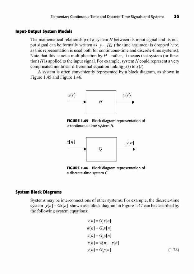
A system is often conveniently represented by a block diagram, as shown inFigure 1.45 and Figure 1.46.
y Hx=
Elementary Continuous-Time and Discrete-Time Signals and Systems 35
FIGURE 1.45 Block diagram representation ofa continuous-time system H.
FIGURE 1.46 Block diagram representation ofa discrete-time system G.
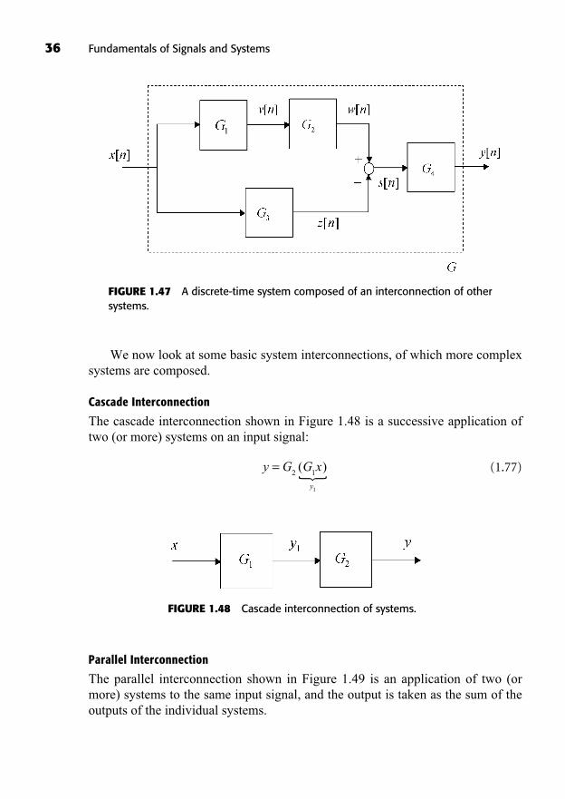
System Block Diagrams
Systems may be interconnections of other systems. For example, the discrete-timesystem shown as a block diagram in Figure 1.47 can be described bythe following system equations:
(1.76)
v n G x n
w n G v n
z n G x n
s n w n
[ ] [ ]
[ ] [ ]
[ ] [ ]
[ ] [ ]
====
1
2
3
zz n
y n G s n
[ ]
[ ] [ ]=4
y n Gx n[ ] [ ]=
36 Fundamentals of Signals and Systems
We now look at some basic system interconnections, of which more complexsystems are composed.
Cascade Interconnection
The cascade interconnection shown in Figure 1.48 is a successive application oftwo (or more) systems on an input signal:
(1.77)y G G xy
=2 1
1
( )�
FIGURE 1.47 A discrete-time system composed of an interconnection of othersystems.
FIGURE 1.48 Cascade interconnection of systems.
Parallel Interconnection
The parallel interconnection shown in Figure 1.49 is an application of two (ormore) systems to the same input signal, and the output is taken as the sum of theoutputs of the individual systems.

(1.78)
Note that because there is no assumption of linearity or any other property forsystems , we are not allowed to write, for example, . Systemproperties will be defined later.
y G G x= +( )1 2
G G1 2,
y G x G x= +1 2
Elementary Continuous-Time and Discrete-Time Signals and Systems 37
FIGURE 1.49 Parallel interconnection of systems.
Feedback Interconnection
The feedback interconnection of two systems as shown in Figure 1.50 is a feedbackof the output of system G1 to its input, through system G2. This interconnection isquite useful in feedback control system analysis and design. In this context, signale is the error between a desired output signal and a direct measurement of the out-put. The equations are
(1.79)
e x G y
y G e
==
2
1
FIGURE 1.50 Feedback interconnection of systems.
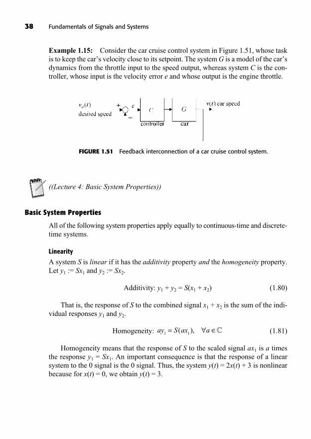
Example 1.15: Consider the car cruise control system in Figure 1.51, whose taskis to keep the car’s velocity close to its setpoint. The system G is a model of the car’sdynamics from the throttle input to the speed output, whereas system C is the con-troller, whose input is the velocity error e and whose output is the engine throttle.
38 Fundamentals of Signals and Systems
FIGURE 1.51 Feedback interconnection of a car cruise control system.
((Lecture 4: Basic System Properties))
Basic System Properties
All of the following system properties apply equally to continuous-time and discrete-time systems.
Linearity
A system S is linear if it has the additivity property and the homogeneity property.Let y1 := Sx1 and y2 := Sx2.
Additivity: y1 + y2 = S(x1 + x2) (1.80)
That is, the response of S to the combined signal x1 + x2 is the sum of the indi-vidual responses y1 and y2.
Homogeneity: (1.81)
Homogeneity means that the response of S to the scaled signal ax1 is a timesthe response y1 = Sx1. An important consequence is that the response of a linearsystem to the 0 signal is the 0 signal. Thus, the system y(t) = 2x(t) + 3 is nonlinearbecause for x(t) = 0, we obtain y(t) = 3.
ay S ax a1 1= ( ), C
The linearity property (additivity and homogeneity combined) is summarized inthe important Principle of Superposition: the response to a linear combination ofinput signals is the same linear combination of the corresponding output signals.
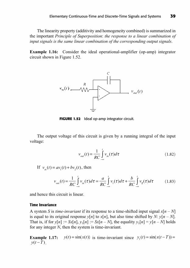
Example 1.16: Consider the ideal operational-amplifier (op-amp) integrator circuit shown in Figure 1.52.
Elementary Continuous-Time and Discrete-Time Signals and Systems 39
FIGURE 1.52 Ideal op-amp integrator circuit.
The output voltage of this circuit is given by a running integral of the inputvoltage:
(1.82)
If , then
(1.83)
and hence this circuit is linear.
Time Invariance
A system S is time-invariant if its response to a time-shifted input signal x[n – N]is equal to its original response y[n] to x[n], but also time shifted by N: y[n – N].That is, if for y[n] := Sx[n], y1[n] := Sx[n – N], the equality y1[n] = y[n – N] holdsfor any integer N, then the system is time-invariant.
Example 1.17: is time-invariant since .y t T( )
y t x t T1( ) sin( ( ))= =y t x t( ) sin( ( ))=
v tRC
v da
RCv d
b
RCv
out in
t t
( ) ( ) ( )= = +1
1 22( )d
t
v t av t bv tin
( ) ( ) ( )= +1 2
v tRC
v dout in
t
( ) ( )=1
On the other hand, the system is not time-invariant (it is time-varying) since .
The time-invariance property of a system makes its analysis easier, as it is suf-ficient to study, for example, the impulse response or the step response starting attime t � 0. Then, we know that the response to a time-shifted impulse would havethe exact same shape, except it would be shifted by the same interval of time as theimpulse.
Memory
A system is memoryless if its output y at time t or n depends only on the input atthat same time.
Examples of memoryless systems:
Resistor: .Conversely, a system has memory if its output at time t or n depends on input
values at some other times.Examples of systems with memory:
Causality
A system is causal if its output at time t or n depends only on past or current val-ues of the input.
An important consequence is that if and , then . This means that a causal system
subjected to two input signals that coincide up to the current time t produces out-puts that also coincide up to time t. This is not the case for noncausal systemsbecause their output up to time t depends on future values of the input signals,which may differ by assumption.
y y t1 2( ) ( ), ( , ]=t( , ]
x x1 2( ) ( ),=y Sx y Sx
1 1 2 2: , := =
y t x dt
( ) ( )=
y n x n x n x n[ ] [ ] [ ] [ ]= + + +1 1
v t Ri t( ) ( )=
y tx t
x t( )
( )
( )=
+1
y n x n[ ] [ ]= 2
y n nx n N n N x n N y n N1[ ] [ ] ( ) [ ] [ ]= =
y n nx n[ ] [ ]=
40 Fundamentals of Signals and Systems
Examples of causal systems: A car does not anticipate its driver’s actions, or the road condition ahead.
Example of a noncausal system:
Bounded-Input Bounded-Output Stability
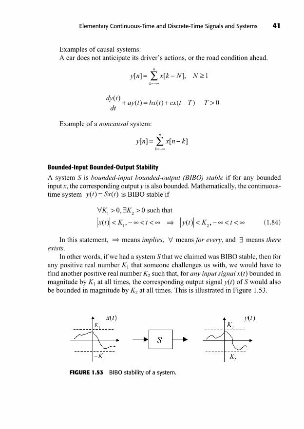
A system S is bounded-input bounded-output (BIBO) stable if for any boundedinput x, the corresponding output y is also bounded. Mathematically, the continuous-time system is BIBO stable if
(1.84)
In this statement, means implies, means for every, and means thereexists.
In other words, if we had a system S that we claimed was BIBO stable, then forany positive real number K1 that someone challenges us with, we would have tofind another positive real number K2 such that, for any input signal x(t) bounded inmagnitude by K1 at all times, the corresponding output signal y(t) of S would alsobe bounded in magnitude by K2 at all times. This is illustrated in Figure 1.53.
> >
< < < <
K K
x t K t y t K1 2
1 2
0 0,
( ) , ( )
such that
,, < <t
y t Sx t( ) ( )=
y n x n kk
n
[ ] [ ]==
T > 0dy t
dtay t bx t cx t T
( )( ) ( ) ( )+ = +
y n x k N Nk
n
[ ] [ ],==
1
Elementary Continuous-Time and Discrete-Time Signals and Systems 41
FIGURE 1.53 BIBO stability of a system.

Example 1.18: A resistor with characteristics is BIBO stable. For allcurrents i(t) bounded by K1 amperes in magnitude, the voltage is bounded by
volts. However, the integrator op-amp circuit previously discussed is notBIBO stable, as a constant input would result in an output that tends to infinity as
.BIBO stability is very important to establish for feedback control systems and
for analog and digital filters.
Invertibility
Recall that a system was defined as a function mapping a set of input signals (do-main) into a set of output signals (co-domain). The range of the system is the sub-set of output signals in the co-domain that are actually possible to get.
It turns out that one can always restrict the co-domain of the system to beequal to its range, thereby making the system onto (surjective). Assuming this isthe case, a system S is invertible if the input signal can always be uniquely recov-ered from the output signal. Mathematically, for , , wehave , which restricts the system to be one-to-one (injective). This meansthat two distinct input signals cannot lead to the same output signal. More gener-ally, functions are invertible if and only if they are both one-to-one and onto.
The inverse system, formally written as S –1 (this is not the arithmetic inverse),is such that the cascade interconnection in Figure 1.54 is equivalent to the identitysystem, which leaves the input unchanged.
y y1 2
y Sx y Sx1 1 2 2= =,x x
1 2
t
K RK2 1=
v t Ri t( ) ( )=
42 Fundamentals of Signals and Systems
FIGURE 1.54 Cascade interconnection of asystem and its inverse.
Example 1.19: The inverse system for y = 2x is just x.Exercise: Check that the inverse system of the discrete-time running sum
is the first-difference system .
SUMMARY
In this chapter, we introduced the following concepts.
A signal was defined as a function of time, either continuous or discrete.A system was defined as a mathematical relationship between an input signaland an output signal.
y n x n x n[ ] [ ] [ ]= 1x k[ ]k
n
=y n[ ] =
1
2y =
Special types of signals were studied: real and complex exponential signals, si-nusoidal signals, impulse and step signals.The main properties of a system were introduced: linearity, memory, causality,time invariance, stability, and invertibility.
TO PROBE FURTHER
There are many introductory textbooks on signals and systems, each organizingand presenting the material in a particular way. See, for example, Oppenheim,Willsky, and Nawab 1997; Haykin & Van Veen, 2002; and Kamen & Heck, 1999.For applications of signal models to specific engineering fields, see, for example,Gold & Morgan, 1999 for speech and signal processing; Haykin, 2000 for modu-lated signals in telecommunications; and Bruce, 2000 for biomedical signals. Forfurther details on system properties, see Chen, 1999.
EXERCISES
Exercises with Solutions
Exercise 1.1
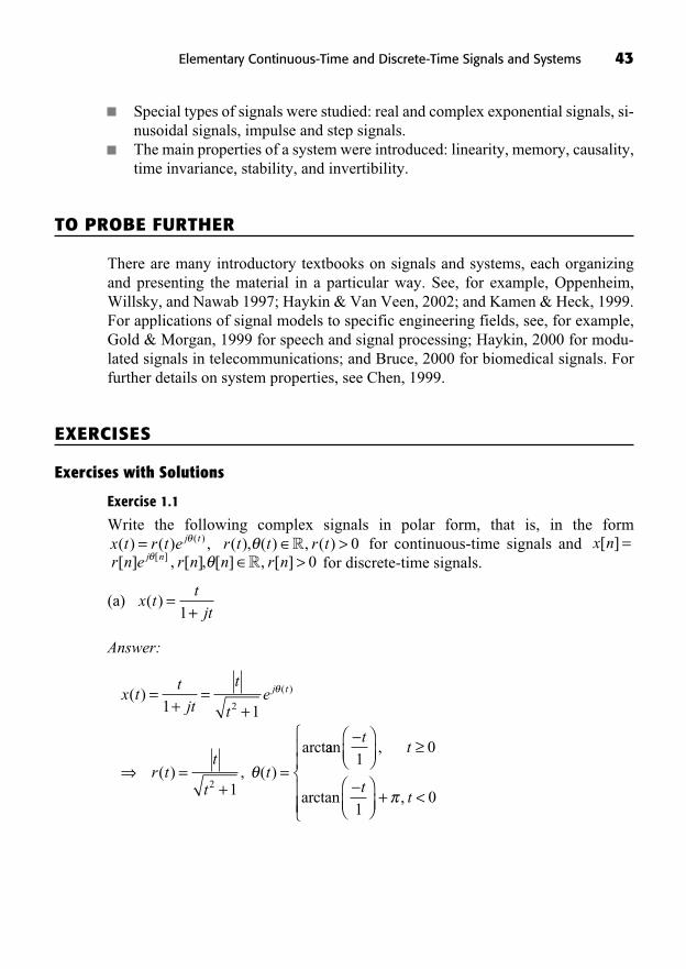
Write the following complex signals in polar form, that is, in the formfor continuous-time signals and
for discrete-time signals.
(a)
Answer:
x tt
jt
t
te
r tt
tt
j t( )
( ) , ( )
( )=+
=+
=+
=
1 1
1
2
2
arctaan
arctan + <
tt
tt
10
10
,
,
x tt
jt( ) =
+1
r n e r n n r nj n[ ] , [ ], [ ] , [ ][ ] >R 0x n[ ] =r t t r t( ), ( ) , ( ) >R 0x t r t e j t( ) ( ) ,( )=
Elementary Continuous-Time and Discrete-Time Signals and Systems 43
(b)
Answer:
Exercise 1.2
Determine whether the following systems are: (1) memoryless, (2) time-invariant, (3)linear, (4) causal, or (5) BIBO stable. Justify your answers.
(a)
Answer:1. Memoryless? No. For example, the output depends on a future
value of the input.2. Time-invariant? No.
3. Linear? Yes. Let . Then, the output of the system with is given by:
4. Causal? No. For example, the output depends on a future valueof the input.
5. Stable? Yes. .
(b)
Answer:1. Memoryless? No. The system has memory since at time t, it uses the past
value of the input .
2. Time-invariant? Yes. .y t Sx t Tx t Tx t T
y t T1 1 1( ) ( )
( )( )
( )= =+
=
x t( )1
y tx tx t
( )( )( )
=+1 1
x n B n y n x n B n[ ] , [ ] [ ] ,< = <1
y x[ ] [ ]0 1=
y Sx
y n x n x n x n
y n
== = +
= +
:
[ ] [ ] [ ] [ ]
[ ]
1 1 11 2
1 yy n2[ ]
x n x n x n[ ] : [ ] [ ]= +1 2
y n Sx n x n y n Sx n x n1 1 1 2 2 21 1[ ] : [ ] [ ], [ ] : [ ] [ ]= = = =
y n Sx n N x n N
x n N x n N1 1
1 1
[ ] [ ] [ ]
[ ( )] [ )]
= =
= + == y n N[ ]
y x[ ] [ ]0 1=
y n x n[ ] [ ]= 1
x n nje ne e n
r n ne n
n j n j
n
[ ] ,
[ ] , [ ]
( )= = >= =
+ +1 2 0
1++ 2
x n nje nn j[ ] ,= >+ 0
44 Fundamentals of Signals and Systems
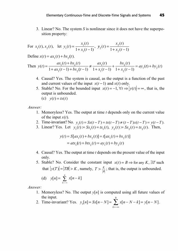
3. Linear? No. The system S is nonlinear since it does not have the superpo-sition property:
4. Causal? Yes. The system is causal, as the output is a function of the pastand current values of the input and x(t) only.
5. Stable? No. For the bounded input , that is, theoutput is unbounded.(c)
Answer:1. Memoryless? Yes. The output at time t depends only on the current value
of the input x(t).2. Time-invariant? No. .3. Linear? Yes. Let . Then,
4. Causal? Yes. The output at time t depends on the present value of the inputonly.
5. Stable? No. Consider the constant input
, namely, ; that is, the output is unbounded.
(d)
Answer:1. Memoryless? No. The output y[n] is computed using all future values of
the input.2. Time-invariant? Yes. .y n Sx n N x n N k y n N
k1
0
[ ] [ ] [ ] [ ]= = ==
x n k[ ]k=
0
y n[ ] =
K
B>T >y T TB K( ) = >that
x t B K T( ) = for any , such
y t S ax t bx t t ax t bx t
atx
( ) [ ( ) ( )] [ ( ) ( )]= + = +
=1 2 1 2
1(( ) ( ) ( ) ( )t btx t ay t by t+ = +2 1 2
y t Sx t tx t y t Sx t tx t1 1 1 2 2 2( ) : ( ) ( ), ( ) : ( ) ( )= = = =y t Sx t T tx t T t T x t T y t T1( ) ( ) ( ) ( ) ( ) ( )= = =
y t tx t( ) ( )=
x t t y t( ) , ( )= =1x t( )1
For let x t x t y tx t
x t1 2 11
11 1( ), ( ), ( )
( )
( ),=
+yy t
x t
x t
x t ax t bx
22
2
1 2
1 1( )
( )
( )
( ) ( )
=+
= +Define (( ).
( )( ) ( )
( )
t
y tax t bx t
ax t bxThen =
++ +
1 2
1 21 1 (( )
( )
( )
( )
( )(
t
ax t
x t
bx t
x tay
++
+=
1 1 1 1 11
1
2
21 tt by t) ( )+ 2
Elementary Continuous-Time and Discrete-Time Signals and Systems 45
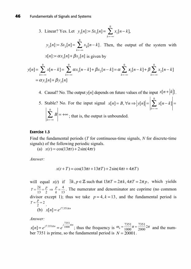
3. Linear? Yes. Let
. Then, the output of the system with
is given by
4. Causal? No. The output y[n] depends on future values of the input .
5. Stable? No. For the input signal
; that is, the output is unbounded.
Exercise 1.3
Find the fundamental periods (T for continuous-time signals, N for discrete-timesignals) of the following periodic signals.
(a)
Answer:
will equal x(t) if , which yields
. The numerator and denominator are coprime (no common
divisor except 1); thus we take , and the fundamental period is
.(b)
Answer:
; thus the frequency is and the num-ber 7351 is prime, so the fundamental period is .N = 20001
0
73511000
73512000
2= =x n e ej n j n[ ] .= =7 351
73511000
x n e j n[ ] .= 7 351
Tp= =2
2
p k= =4 13,
Tk p p
k= = =2
13 24
13
= =k p T k T p, ,Z such that 13 2 4 2
x t T t T t T( ) cos( ) sin( )+ = + + +13 13 2 4 4
x t t t( ) cos( ) sin( )= +13 2 4
Bk
= +=
0
x n B n y n x n kk
[ ] , [ ] [ ]= = ==
0
x n k[ ]+
y n x n k x n k x n kk k
[ ] [ ] [ ] [ ]= = + == =
0
1 2
0
xx n k x n k
y n y nk k
1
0
2
0
1 2
[ ] [ ]
[ ] [ ]
+
= += =
x n x n x n[ ] : [ ] [ ]= +1 2
y n Sx n x2 2[ ] : [ ]= = 22
0
[ ]n kk=
y n Sx n x n kk
1 1 1
0
[ ] : [ ] [ ],= ==
46 Fundamentals of Signals and Systems
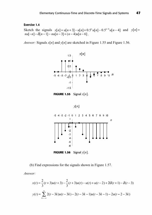
Exercise 1.4
Sketch the signals and .
Answer: Signals x[n] and y[n] are sketched in Figure 1.55 and Figure 1.56.
nu n n nu n n u n[ ] [ ] [ ] ( ) [ ]+1 3 4 6y n[ ] =x n u n u n u n u nn n[ ] [ ] [ ] . [ ] . [ ]= + +3 0 5 0 5 44
Elementary Continuous-Time and Discrete-Time Signals and Systems 47
FIGURE 1.55 Signal x[n].
FIGURE 1.56 Signal y[n].
(b) Find expressions for the signals shown in Figure 1.57.
Answer:
y t t k u t k t k u t k u t( ) ( ) ( ) ( ) ( ) (= 2 3 3 2 3 1 3 1 2=
2 3kk
)
x t t u t t u t u t u t( ) ( ) ( ) ( ) ( ) ( ) ( )= + + + + +2
33 3
2
33 2 22 1 3( ) ( )t t+
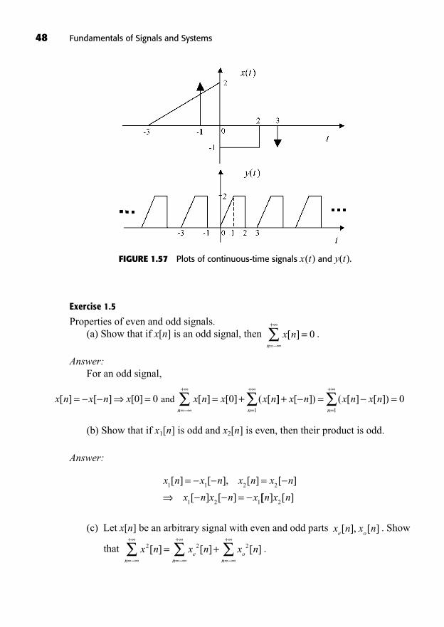
48 Fundamentals of Signals and Systems
Exercise 1.5
Properties of even and odd signals.(a) Show that if x[n] is an odd signal, then .
Answer:For an odd signal,
(b) Show that if x1[n] is odd and x2[n] is even, then their product is odd.
Answer:
(c) Let x[n] be an arbitrary signal with even and odd parts . Show
that .x n x n x nn
en
on
2 2 2[ ] [ ] [ ]=
+
=
+
=
+
= +
x n x ne o[ ], [ ]
x n x n x n x n
x n x n x1 1 2 2
1 2 1
[ ] [ ], [ ] [ ]
[ ] [ ]
= == [[ ] [ ]n x n
2
x n x n x x n x x nn
[ ] [ ] [ ] [ ] [ ] ( [= = = +=
+
0 0 0and ]] [ ]) ( [ ] [ ])+ = ==
+
=
+
x n x n x nn n1 1
0
x nn
[ ]=
+
= 0
FIGURE 1.57 Plots of continuous-time signals x(t) and y(t).

Elementary Continuous-Time and Discrete-Time Signals and Systems 49
Answer:
(d) Similarly, show that .
Answer:
Exercises
Exercise 1.6
Write the following complex signals in rectangular form: for continuous-time signals and for
discrete-time signals.(a)(b)
Exercise 1.7
Use the sampling property of the impulse to simplify the following expressions.(a)
(b)
(c)
Answer:
x n n n kk
[ ] cos( . ) [ ]==
0 2 100
x t t t kk
( ) sin( ) ( )==
20
x t e t tt( ) cos( ) ( )= 10
x t e u t e u tj t j t( ) ( ) ( )( )= + +2
x t e j t( ) ( )= +2 3
x n a n jb n a n b n[ ] [ ] [ ], [ ], [ ]= + Rb t( ) Rx t a t jb t a t( ) ( ) ( ), ( ),= +
x t dt x t x t dt x t dte o e
2 2 2( ) ( ( ) ( )) ( )+ +
= + =+ +
+ +2
0
2x t x t dt x t dte o o( ) ( ) ( )
� ��� ���
+
+ +
= +x t dt x t dte o
2 2( ) ( )
x t dt x t dt x t dte o2 2 2( ) ( ) ( )
+ + +
= +
x n x n x n x nn
e on
en
2 2 2[ ] ( [ ] [ ]) [ ]=
+
=
+
=
= + =+
=
+
=
=
+ +2
0
2x n x n x ne o
no
n
[ ] [ ] [ ]� ��� ���
+
=
+
=
+
= +x n x ne
no
n
2 2[ ] [ ]
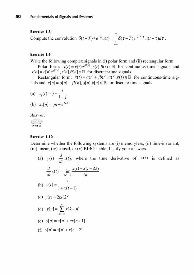
50 Fundamentals of Signals and Systems
Exercise 1.8
Compute the convolution .
Exercise 1.9
Write the following complex signals in (i) polar form and (ii) rectangular form.Polar form: for continuous-time signals and
for discrete-time signals.Rectangular form: for continuous-time sig-
nals and for discrete-time signals.
(a)
(b)
Answer:
Exercise 1.10
Determine whether the following systems are (i) memoryless, (ii) time-invariant,(iii) linear, (iv) causal, or (v) BIBO stable. Justify your answers.
(a) , where the time derivative of is defined as
.
(b)
(c)
(d)
(e)
(f) y n x n x n[ ] [ ] [ ]= + 2
y n x n nx n[ ] [ ] [ ]= + +1
y n x k nk
n
[ ] [ ]==
y t tx t( ) ( )= 2 2
y tt
x t( )
( )=
+1 1
ddt
x tx t x t t
tt( ) : lim
( ) ( )=0
x t( )y tddt
x t( ) ( )=
x n jn e j n2
2[ ] = +
x t jt
j1 1( ) = +
x n a n jb n a n b n[ ] [ ] [ ], [ ], [ ]= + Rx t a t jb t a t b t( ) ( ) ( ), ( ), ( )= + R
x n r n e r n nj n[ ] [ ] , [ ], [ ][ ]= Rx t r t e r t tj t( ) ( ) , ( ), ( )( )= R
( ) ( ) ( ) ( )( )t T e u t T e u t dt t=2 2
Elementary Continuous-Time and Discrete-Time Signals and Systems 51
Exercise 1.11
Find the fundamental periods and fundamental frequencies of the following peri-odic signal.
(a)
(b) . Sketch this
signal.
Answer:
x t e t k u t k u t kt k( ) cos ( ) ( ) ( )( )= ( )2 4 2 2 2 1=k
x n n e j n[ ] cos( . ) .= 0 01 0 13

This page intentionally left blank

53
Linear Time-InvariantSystems
2
In This Chapter
Discrete-Time LTI Systems: The Convolution SumContinuous-Time LTI Systems: The Convolution IntegralProperties of Linear Time-Invariant SystemsSummaryTo Probe FurtherExercises
((Lecture 5: LTI Systems; Convolution Sum ))
Many physical processes can be represented by, and successfully analyzedwith, linear time-invariant (LTI) systems as models. For example, both aDC motor or a liquid mixing tank have constant dynamical behavior
(time-invariant) and can be modeled by linear differential equations. Filter circuitsdesigned with operational amplifiers are usually modeled as LTI systems for analy-sis. LTI models are also extremely useful for design. A process control engineerwould typically design a level controller for the mixing tank based on a set of lin-earized, time-invariant differential equations. DC motors are often used in indus-trial robots and may be controlled using simple LTI controllers designed using LTImodels of the motors and the robot.
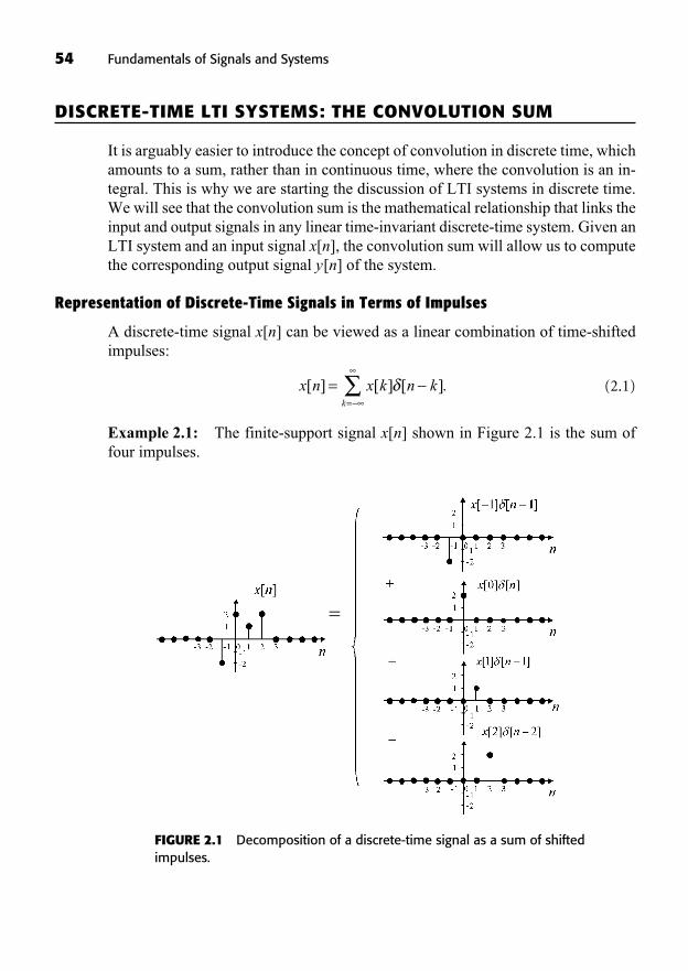
54 Fundamentals of Signals and Systems
DISCRETE-TIME LTI SYSTEMS: THE CONVOLUTION SUM
It is arguably easier to introduce the concept of convolution in discrete time, whichamounts to a sum, rather than in continuous time, where the convolution is an in-tegral. This is why we are starting the discussion of LTI systems in discrete time.We will see that the convolution sum is the mathematical relationship that links theinput and output signals in any linear time-invariant discrete-time system. Given anLTI system and an input signal x[n], the convolution sum will allow us to computethe corresponding output signal y[n] of the system.
Representation of Discrete-Time Signals in Terms of Impulses
A discrete-time signal x[n] can be viewed as a linear combination of time-shiftedimpulses:
(2.1)
Example 2.1: The finite-support signal x[n] shown in Figure 2.1 is the sum offour impulses.
x n x k n kk
[ ] [ ] [ ].==
FIGURE 2.1 Decomposition of a discrete-time signal as a sum of shiftedimpulses.
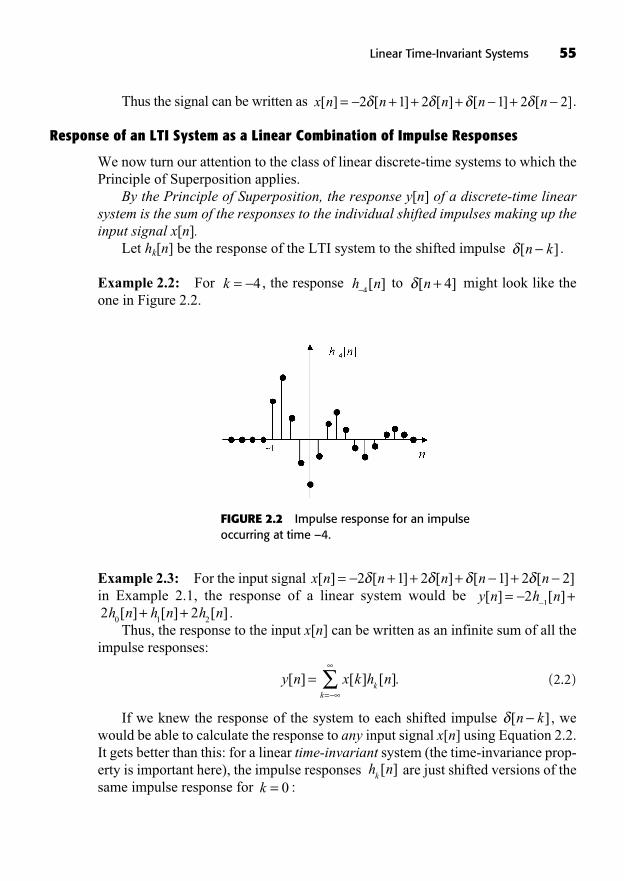
Thus the signal can be written as .
Response of an LTI System as a Linear Combination of Impulse Responses
We now turn our attention to the class of linear discrete-time systems to which thePrinciple of Superposition applies.
By the Principle of Superposition, the response y[n] of a discrete-time linearsystem is the sum of the responses to the individual shifted impulses making up theinput signal x[n].
Let hk[n] be the response of the LTI system to the shifted impulse .
Example 2.2: For , the response to might look like theone in Figure 2.2.
[ ]n + 4h n4[ ]k = 4
[ ]n k
x n n n n n[ ] [ ] [ ] [ ] [ ]= + + + +2 1 2 1 2 2
Linear Time-Invariant Systems 55
FIGURE 2.2 Impulse response for an impulseoccurring at time –4.
Example 2.3: For the input signal in Example 2.1, the response of a linear system would be
.Thus, the response to the input x[n] can be written as an infinite sum of all the
impulse responses:
(2.2)
If we knew the response of the system to each shifted impulse , wewould be able to calculate the response to any input signal x[n] using Equation 2.2.It gets better than this: for a linear time-invariant system (the time-invariance prop-erty is important here), the impulse responses are just shifted versions of thesame impulse response for :k = 0
h nk[ ]
[ ]n k
y n x k h nk
k
[ ] [ ] [ ].==
h n h n h n[ ] [ ] [ ]+ +2 20 1 2
y n h n[ ] [ ]= +21
x n n n n n[ ] [ ] [ ] [ ] [ ]= + + + +2 1 2 1 2 2
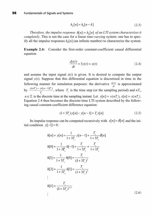
56 Fundamentals of Signals and Systems
(2.3)
Therefore, the impulse response of an LTI system characterizes itcompletely. This is not the case for a linear time-varying system: one has to spec-ify all the impulse responses hk[n] (an infinite number) to characterize the system.
Example 2.4: Consider the first-order constant-coefficient causal differentialequation
(2.4)
and assume the input signal x(t) is given. It is desired to compute the output signal y(t). Suppose that this differential equation is discretized in time in the
following manner for simulation purposes: the derivative is approximated
by , where is the time step (or the sampling period) and nTs,
is the discrete time at the sampling instant. Let .Equation 2.4 then becomes the discrete-time LTI system described by the follow-ing causal constant-coefficient difference equation:
(2.5)
Its impulse response can be computed recursively with and the ini-tial condition :
(2.6)
h n y nT
y nT
Tn
h
s
s
s
[ ] [ ] [ ] [ ]
[ ]
= =+
++
=+
1
1 31
1 3
01
1 3TTh
T
T
T
T
hT
hT
s
s
s
s
s
s
s
[ ]
[ ] [ ](
++
=+
=+
=
11 3 1 3
11
1 30
11 3
21
1 31
1 3
2
3
+
=+
=+
=
T
hT
hT
T
h kT
s
s
s
s
s
)
[ ] [ ]( )
[ ](
�
11 3 1+ +Ts
k)
�
y[ ] =1 0x n n[ ] [ ]=
( ) [ ] [ ] [ ]1 3 1+ =T y n y n T x ns s
y n y nT x n x nTs s
[ ] : ( ), [ ] : ( )= =n ZT
s
y nT y n T
Ts s
s
( ) (( ) )1
dy t
dt
( )
dy t
dty t x t
( )( ) ( )+ =3
h n h n[ ] : [ ]=0
h n h n kk[ ] [ ]=
0
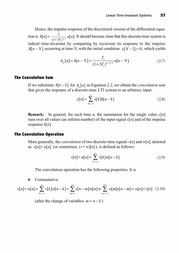
Hence, the impulse response of the discretized version of the differential equa-
tion is . It should become clear that this discrete-time system is
indeed time-invariant by computing by recursion its response to the impulseoccurring at time N, with the initial condition , which yields
(2.7)
The Convolution Sum
If we substitute for in Equation 2.2, we obtain the convolution sumthat gives the response of a discrete-time LTI system to an arbitrary input.
(2.8)
Remark: In general, for each time n, the summation for the single value y[n]runs over all values (an infinite number) of the input signal x[n] and of the impulseresponse h[n].
The Convolution Operation
More generally, the convolution of two discrete-time signals v[n] and w[n], denotedas (or sometimes ), is defined as follows:
(2.9)
The convolution operation has the following properties. It is
Commutative:
(2.10)
(after the change of variables )m n k=
v n w n v k w n k v n m w mk m
[ ] [ ] [ ] [ ] [ ] [ ]= == =
== ==
+
w m v n m w n v nm
[ ] [ ] [ ] [ ]
v n w n v k w n kk
[ ] [ ] [ ] [ ].==
( )[ ]v w nv n w n[ ] [ ]
y n x k h n kk
[ ] [ ] [ ]==
h nk[ ]h n k[ ]
h n h n NT
Tu n N
Ns
sn N
[ ] [ ]( )
[ ].= =+ +1 3 1
y N[ ] =1 0[ ]n N
u n[ ]T
Ts
sn( )+ +1 3 1
h n[ ] =
Linear Time-Invariant Systems 57
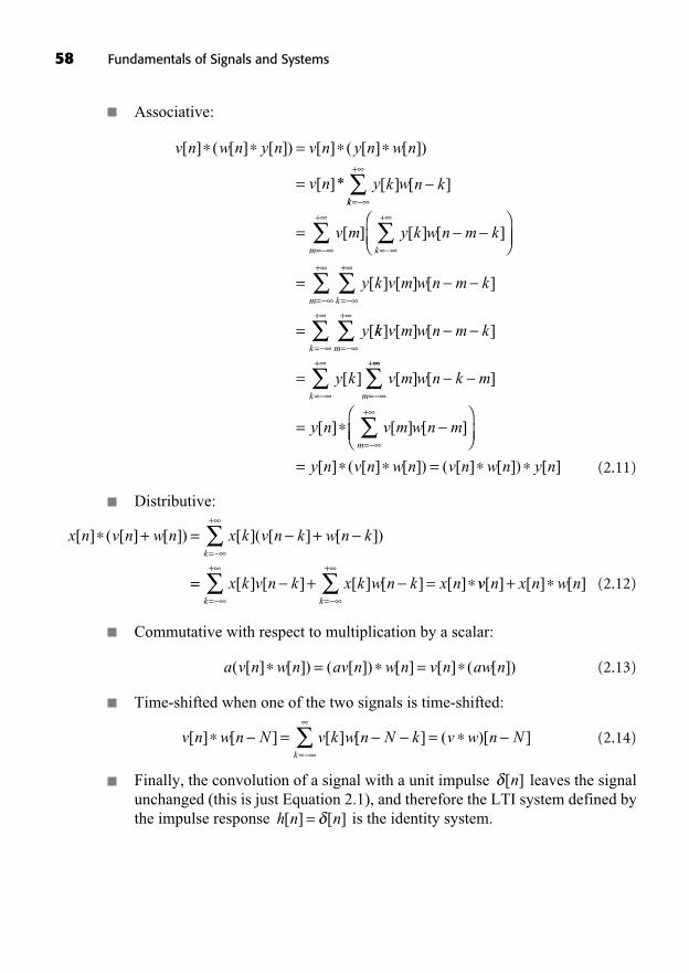
Associative:
(2.11)
Distributive:
(2.12)
Commutative with respect to multiplication by a scalar:
(2.13)
Time-shifted when one of the two signals is time-shifted:
(2.14)
Finally, the convolution of a signal with a unit impulse leaves the signalunchanged (this is just Equation 2.1), and therefore the LTI system defined bythe impulse response is the identity system.h n n[ ] [ ]=
[ ]n
v n w n N v k w n N k v w n Nk
[ ] [ ] [ ] [ ] ( )[ ]= ==
a v n w n av n w n v n aw n( [ ] [ ]) ( [ ]) [ ] [ ] ( [ ])= =
x n v n w n x k v n k w n kk
[ ] ( [ ] [ ]) [ ]( [ ] [ ])+ = +=
+
== + ==
+
=
+
x k v n k x k w n k x nk k
[ ] [ ] [ ] [ ] [ ] vv n x n w n[ ] [ ] [ ]+
v n w n y n v n y n w n
v n y k
[ ] ( [ ] [ ]) [ ] ( [ ] [ ])
[ ]* [ ]
=
=kk
k
w n k
v m y k w n m k
=
+
=
+
=
[ ]
[ ] [ ] [ ]
=
=
=
+
=
+
=
+
m
km
y k v m w n m k
y
[ ] [ ] [ ]
[kk v m w n m k
y k v m
mk
m
] [ ] [ ]
[ ] [ ]
=
+
=
+
=
+
==
+
=
+
=
w n k m
y n v m w n m
k
m
[ ]
[ ] [ ] [ ]
= =y n v n w n v n w n y n[ ] ( [ ] [ ]) ( [ ] [ ]) [ ]
58 Fundamentals of Signals and Systems
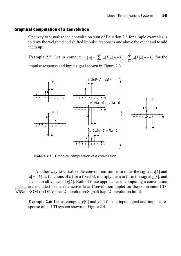
Graphical Computation of a Convolution
One way to visualize the convolution sum of Equation 2.8 for simple examples isto draw the weighted and shifted impulse responses one above the other and to addthem up.
Example 2.5: Let us compute for the
impulse response and input signal shown in Figure 2.3.
x k h n k[ ] [ ]0k=0
2
x k h n k[ ] [ ] =k=
y n[ ] =
Linear Time-Invariant Systems 59
FIGURE 2.3 Graphical computation of a convolution.
Another way to visualize the convolution sum is to draw the signals x[k] andas functions of k (for a fixed n), multiply them to form the signal g[k], and
then sum all values of g[k]. Both of these approaches to computing a convolutionare included in the interactive Java Convolution applet on the companion CD-ROM (in D:\Applets\Convolution\SignalGraph\Convolution.html).
Example 2.6: Let us compute y[0] and y[1] for the input signal and impulse re-sponse of an LTI system shown in Figure 2.4.
h n k[ ]
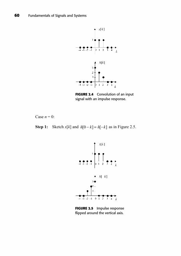
60 Fundamentals of Signals and Systems
Case n = 0:
Step 1: Sketch x[k] and as in Figure 2.5.h k h k[ ] [ ]0 =
FIGURE 2.4 Convolution of an inputsignal with an impulse response.
FIGURE 2.5 Impulse responseflipped around the vertical axis.
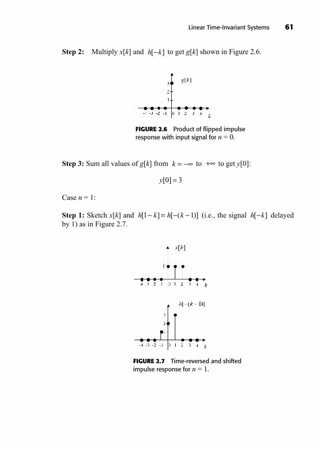
Step 2: Multiply x[k] and to get g[k] shown in Figure 2.6.h k[ ]
Linear Time-Invariant Systems 61
FIGURE 2.6 Product of flipped impulseresponse with input signal for n = 0.
Step 3: Sum all values of g[k] from to to get y[0]:
Case n = 1:
Step 1: Sketch x[k] and (i.e., the signal delayedby 1) as in Figure 2.7.
h k[ ]h k h k[ ] [ ( )]1 1=
y[ ]0 3=
+k =
FIGURE 2.7 Time-reversed and shiftedimpulse response for n = 1.
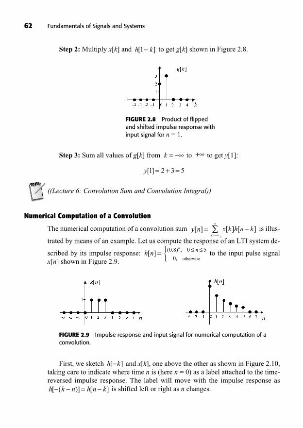
Step 2: Multiply x[k] and to get g[k] shown in Figure 2.8.h k[ ]1
62 Fundamentals of Signals and Systems
FIGURE 2.8 Product of flippedand shifted impulse response withinput signal for n = 1.
Step 3: Sum all values of g[k] from to to get y[1]:
((Lecture 6: Convolution Sum and Convolution Integral))
Numerical Computation of a Convolution
The numerical computation of a convolution sum is illus-
trated by means of an example. Let us compute the response of an LTI system de-
scribed by its impulse response: to the input pulse signalx[n] shown in Figure 2.9.
nn( . ) ,
,
0 8 0 5
0 otherwiseh n[ ] =
x k h n k[ ] [ ]k=
y n[ ] =
y[ ]1 2 3 5= + =
+k =
FIGURE 2.9 Impulse response and input signal for numerical computation of aconvolution.
First, we sketch and x[k], one above the other as shown in Figure 2.10,taking care to indicate where time n is (here n = 0) as a label attached to the time-reversed impulse response. The label will move with the impulse response as
is shifted left or right as n changes.h k n h n k[ ( )] [ ]=
h k[ ]
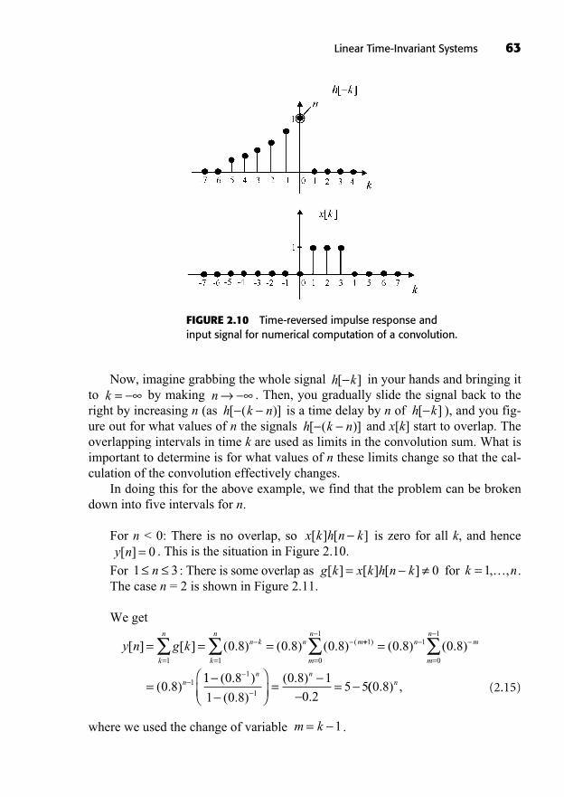
Now, imagine grabbing the whole signal in your hands and bringing itto by making . Then, you gradually slide the signal back to theright by increasing n (as is a time delay by n of ), and you fig-ure out for what values of n the signals and x[k] start to overlap. Theoverlapping intervals in time k are used as limits in the convolution sum. What isimportant to determine is for what values of n these limits change so that the cal-culation of the convolution effectively changes.
In doing this for the above example, we find that the problem can be brokendown into five intervals for n.
For n < 0: There is no overlap, so is zero for all k, and hence. This is the situation in Figure 2.10.
For : There is some overlap as for .The case n = 2 is shown in Figure 2.11.
We get
(2.15)
where we used the change of variable .m k= 1
y n g kk
nn k
k
nn m[ ] [ ] ( . ) ( . ) ( . ) (= = =
= =1 1
0 8 0 8 0 8 ++
= =
=
=
1
0
11
0
1
1
0 8 0 8
0 8
) ( . ) ( . )
( . )
m
nn m
m
n
n 11 0 8
1 0 8
0 8 1
0 25 5
1
1= =
( . )
( . )
( . )
.
n n
(( . ) ,0 8 n
k n= 1, ,…g k x k h n k[ ] [ ] [ ]= 01 3n
y n[ ] = 0x k h n k[ ] [ ]
h k n[ ( )]h k[ ]h k n[ ( )]
nk =h k[ ]
Linear Time-Invariant Systems 63
FIGURE 2.10 Time-reversed impulse response andinput signal for numerical computation of a convolution.
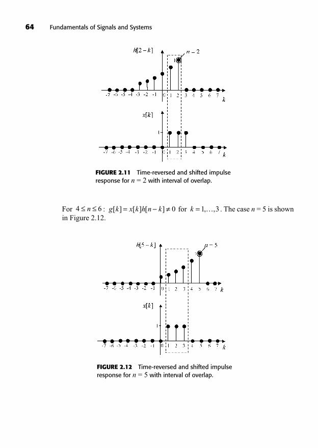
64 Fundamentals of Signals and Systems
For : for . The case n = 5 is shownin Figure 2.12.
k = 1 3, ,…g k x k h n k[ ] [ ] [ ]= 04 6n
FIGURE 2.11 Time-reversed and shifted impulseresponse for n = 2 with interval of overlap.
FIGURE 2.12 Time-reversed and shifted impulseresponse for n = 5 with interval of overlap.

We get
(2.16)
where we used the change of variables .For : for (see Figure 2.13).n k5 3g k x k h n k[ ] [ ] [ ]= 07 8n
m k= 1
y n g kk
n k
k
n m[ ] [ ] ( . ) ( . ) ( . ) (= = == =1
3
1
3
0 8 0 8 0 8 ++
= =
=
=
1
0
21
0
2
1
0 8 0 8
0 81 0
) ( . ) ( . )
( . )(
m
n m
m
n .. )
( . )
( . ) ( . )
.
8
1 0 8
0 8 0 8
0 2
1 3
1
3
= =n n
55 0 8 5 0 8 4 7656 0 83( . ) ( . ) . ( . ) ,n n n=
Linear Time-Invariant Systems 65
FIGURE 2.13 Time-reversed and shifted impulseresponse for n = 7 with interval of overlap.
We have
(2.17)
where we used the change of variables .For : the two signals do not overlap, so .y n[ ] = 0x k h n k[ ], [ ]n 9
m k n= ( )5
y n g kk n
n k
k n
n m[ ] [ ] ( . ) ( . ) (= = == =
+
5
3
5
3
0 8 0 8 nn
m
nm
m
n
= =
=
=
5
0
85
0
8
5
0 8 0 8
0 81
) ( . ) ( . )
( . )(00 8
1 0 8
0 8 0 8
0
1 9
1
6 3. )
( . )
( . ) ( . )=n n
..( . ) ( . ) ,
25 0 8 5 0 83 6= n
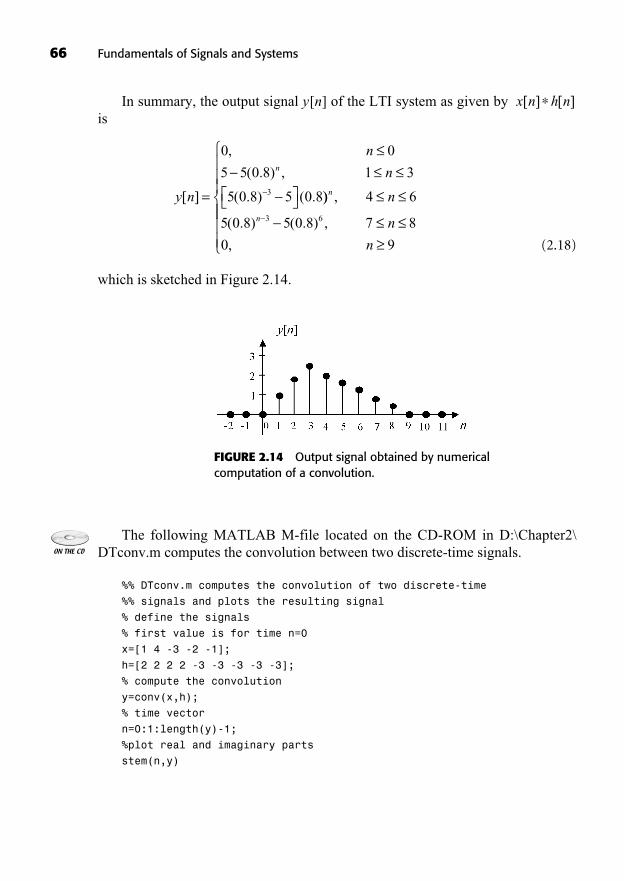
In summary, the output signal y[n] of the LTI system as given by is
(2.18)
which is sketched in Figure 2.14.
y n
n
nn
[ ]
,
( . ) ,
( . ) ( .=
0 0
5 5 0 8 1 3
5 0 8 5 0 83 )) ,
( . ) ( . ) ,
,
n
n
n
n
n
4 6
5 0 8 5 0 8 7 8
0 9
3 6
x n h n[ ] [ ]
66 Fundamentals of Signals and Systems
FIGURE 2.14 Output signal obtained by numericalcomputation of a convolution.
The following MATLAB M-file located on the CD-ROM in D:\Chapter2\DTconv.m computes the convolution between two discrete-time signals.
%% DTconv.m computes the convolution of two discrete-time
%% signals and plots the resulting signal
% define the signals
% first value is for time n=0
x=[1 4 -3 -2 -1];
h=[2 2 2 2 -3 -3 -3 -3 -3];
% compute the convolution
y=conv(x,h);
% time vector
n=0:1:length(y)-1;
%plot real and imaginary parts
stem(n,y)
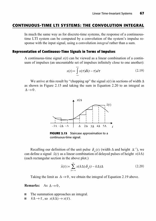
CONTINUOUS-TIME LTI SYSTEMS: THE CONVOLUTION INTEGRAL
In much the same way as for discrete-time systems, the response of a continuous-time LTI system can be computed by a convolution of the system’s impulse re-sponse with the input signal, using a convolution integral rather than a sum.
Representation of Continuous-Time Signals in Terms of Impulses
A continuous-time signal x(t) can be viewed as a linear combination of a contin-uum of impulses (an uncountable set of impulses infinitely close to one another):
(2.19)
We arrive at this result by “chopping up” the signal x(t) in sections of width as shown in Figure 2.15 and taking the sum in Equation 2.20 to an integral as
.0
x t x t d( ) ( ) ( )=+
Linear Time-Invariant Systems 67
FIGURE 2.15 Staircase approximation to acontinuous-time signal.
Recalling our definition of the unit pulse (width and height ), wecan define a signal as a linear combination of delayed pulses of height (each rectangular section in the above plot.)
(2.20)
Taking the limit as , we obtain the integral of Equation 2.19 above.
Remarks: As ,
The summation approaches an integral., so .x k x( ) ( )k
0
0
ˆ( ) : ( ) ( )x t x k t kk
==
x k( )ˆ( )x t
1( )t
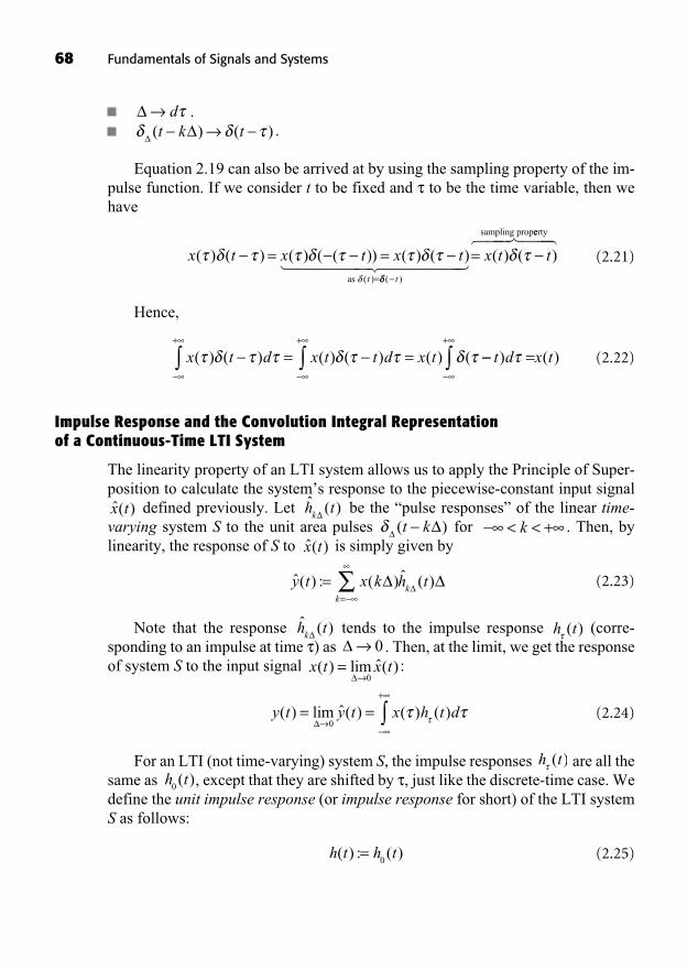
..
Equation 2.19 can also be arrived at by using the sampling property of the im-pulse function. If we consider t to be fixed and to be the time variable, then wehave
(2.21)
Hence,
(2.22)
Impulse Response and the Convolution Integral Representation of a Continuous-Time LTI System
The linearity property of an LTI system allows us to apply the Principle of Super-position to calculate the system’s response to the piecewise-constant input signal
defined previously. Let be the “pulse responses” of the linear time-varying system S to the unit area pulses for . Then, bylinearity, the response of S to is simply given by
(2.23)
Note that the response tends to the impulse response (corre-sponding to an impulse at time ) as . Then, at the limit, we get the responseof system S to the input signal :
(2.24)
For an LTI (not time-varying) system S, the impulse responses are all thesame as , except that they are shifted by , just like the discrete-time case. Wedefine the unit impulse response (or impulse response for short) of the LTI systemS as follows:
(2.25)h t h t( ) : ( )=0
h t0( )
h t( )
y t y t x h t d( ) lim ˆ( ) ( ) ( )= =+
0
x t x t( ) lim ˆ( )=0
0h t( )ˆ ( )h t
k
ˆ( ) : ( ) ˆ ( )y t x k h tk
k=
=
ˆ( )x t< < +k( )t k
ˆ ( )h tk
ˆ( )x t
x t d x t t d x t( ) ( ) ( ) ( ) ( ) (= =+ +
=+
t d x t) ( )
x t x t x tt
( ) ( ) ( ) ( ( )) ( ) ( )( )
= ==as ( )
( ) ( )=t
x t t� ������ ������
sampling propeerty� ��� ��
( ) ( )t k td
68 Fundamentals of Signals and Systems
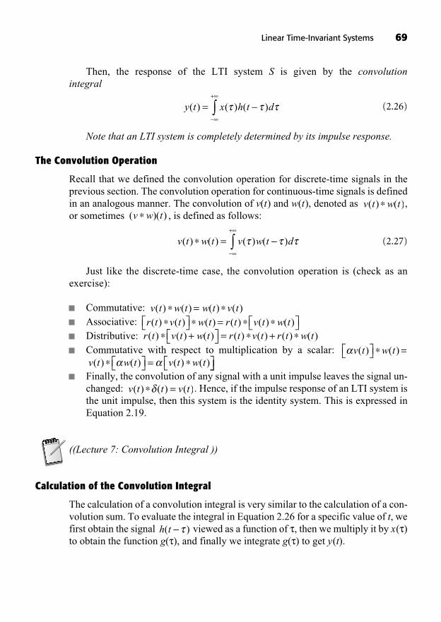
Then, the response of the LTI system S is given by the convolution integral
(2.26)
Note that an LTI system is completely determined by its impulse response.
The Convolution Operation
Recall that we defined the convolution operation for discrete-time signals in theprevious section. The convolution operation for continuous-time signals is definedin an analogous manner. The convolution of v(t) and w(t), denoted as ,or sometimes , is defined as follows:
(2.27)
Just like the discrete-time case, the convolution operation is (check as an exercise):
Commutative: Associative: Distributive: Commutative with respect to multiplication by a scalar:
Finally, the convolution of any signal with a unit impulse leaves the signal un-changed: . Hence, if the impulse response of an LTI system isthe unit impulse, then this system is the identity system. This is expressed inEquation 2.19.
((Lecture 7: Convolution Integral ))
Calculation of the Convolution Integral
The calculation of a convolution integral is very similar to the calculation of a con-volution sum. To evaluate the integral in Equation 2.26 for a specific value of t, wefirst obtain the signal viewed as a function of , then we multiply it by x( )to obtain the function g( ), and finally we integrate g( ) to get y(t).
h t( )
v t t v t( ) ( ) ( )=
v t w t v t w t( ) ( ) ( ) ( )=v t w t( ) ( ) =
r t v t w t r t v t r t w t( ) ( ) ( ) ( ) ( ) ( ) ( )+ = +r t v t w t r t v t w t( ) ( ) ( ) ( ) ( ) ( )=v t w t w t v t( ) ( ) ( ) ( )=
v t w t v w t d( ) ( ) ( ) ( )=+
( )( )v w tv t w t( ) ( )
y t x h t d( ) ( ) ( )=+
Linear Time-Invariant Systems 69
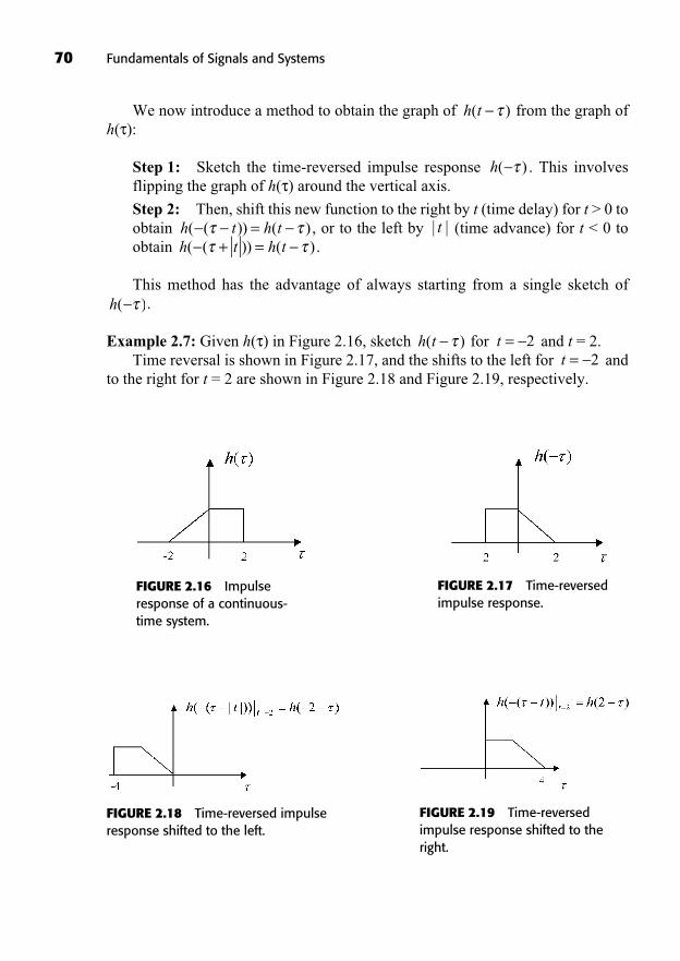
We now introduce a method to obtain the graph of from the graph ofh( ):
Step 1: Sketch the time-reversed impulse response . This involvesflipping the graph of h( ) around the vertical axis.
Step 2: Then, shift this new function to the right by t (time delay) for t > 0 toobtain , or to the left by (time advance) for t < 0 toobtain .
This method has the advantage of always starting from a single sketch of.
Example 2.7: Given h( ) in Figure 2.16, sketch for and t = 2.Time reversal is shown in Figure 2.17, and the shifts to the left for and
to the right for t = 2 are shown in Figure 2.18 and Figure 2.19, respectively.t = 2
t = 2h t( )
h( )
h t h t( ( )) ( )+ =| |th t h t( ( )) ( )=
h( )
h t( )
70 Fundamentals of Signals and Systems
FIGURE 2.16 Impulseresponse of a continuous-time system.
FIGURE 2.17 Time-reversedimpulse response.
FIGURE 2.18 Time-reversed impulseresponse shifted to the left.
FIGURE 2.19 Time-reversedimpulse response shifted to theright.
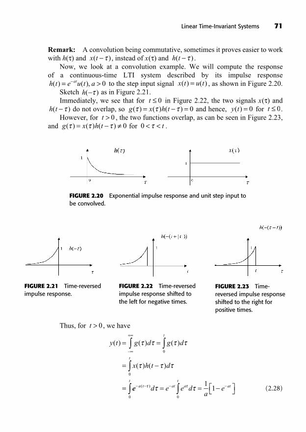
Remark: A convolution being commutative, sometimes it proves easier to workwith h( ) and , instead of x( ) and .
Now, we look at a convolution example. We will compute the response of a continuous-time LTI system described by its impulse response
to the step input signal , as shown in Figure 2.20.Sketch as in Figure 2.21.Immediately, we see that for in Figure 2.22, the two signals x( ) and
do not overlap, so and hence, for .However, for , the two functions overlap, as can be seen in Figure 2.23,
and for .0 < < tg x h t( ) ( ) ( )= 0t > 0
t 0y t( ) = 0g x h t( ) ( ) ( )= = 0h t( )t 0
h( )x t u t( ) ( )=h t e u t aat( ) ( ),= > 0
h t( )x t( )
Linear Time-Invariant Systems 71
FIGURE 2.21 Time-reversedimpulse response.
FIGURE 2.22 Time-reversedimpulse response shifted tothe left for negative times.
FIGURE 2.23 Time-reversed impulse responseshifted to the right forpositive times.
FIGURE 2.20 Exponential impulse response and unit step input tobe convolved.
Thus, for , we have
(2.28)
y t g d g d
x h t d
t
t
( ) ( ) ( )
( ) ( )
= =
=
=
+
0
0
ee d e e da
ea tt
at at
at= =( )
0 0
11
t > 0
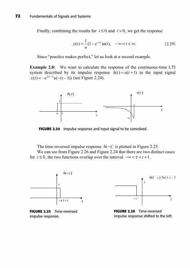
Finally, combining the results for and , we get the response
(2.29)
Since “practice makes perfect,” let us look at a second example.
Example 2.8: We want to calculate the response of the continuous-time LTI system described by its impulse response to the input signal
(see Figure 2.24).x t e u tt( ) ( ( ))( )= 2 1 1h t u t( ) ( )= +1
y ta
e u t tat( ) ( ) ( ), .= < <1
1
t > 0t 0
72 Fundamentals of Signals and Systems
FIGURE 2.24 Impulse response and input signal to be convolved.
The time-reversed impulse response is plotted in Figure 2.25.We can see from Figure 2.26 and Figure 2.24 that there are two distinct cases:
for , the two functions overlap over the interval .< < +t 1t 0
h( )
FIGURE 2.25 Time-reversedimpulse response.
FIGURE 2.26 Time-reversedimpulse response shifted to the left.
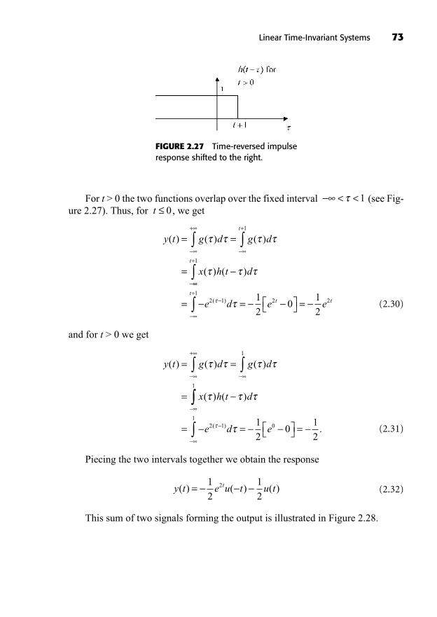
For t > 0 the two functions overlap over the fixed interval (see Fig-ure 2.27). Thus, for , we get
(2.30)
and for t > 0 we get
(2.31)
Piecing the two intervals together we obtain the response
(2.32)
This sum of two signals forming the output is illustrated in Figure 2.28.
y t e u t u tt( ) ( ) ( )=1
2
1
22
y t g d g d
x h t d
( ) ( ) ( )
( ) ( )
= =
=
+ 1
1
= = =e d e2 11
01
20
1
2( ) .
y t g d g d
x h t d
t
( ) ( ) ( )
( ) ( )
= =
=
+ +1
+
+
= = =
t
tt te d e e
1
2 11
2 21
20
1
2( )
t 0< <1
Linear Time-Invariant Systems 73
FIGURE 2.27 Time-reversed impulseresponse shifted to the right.
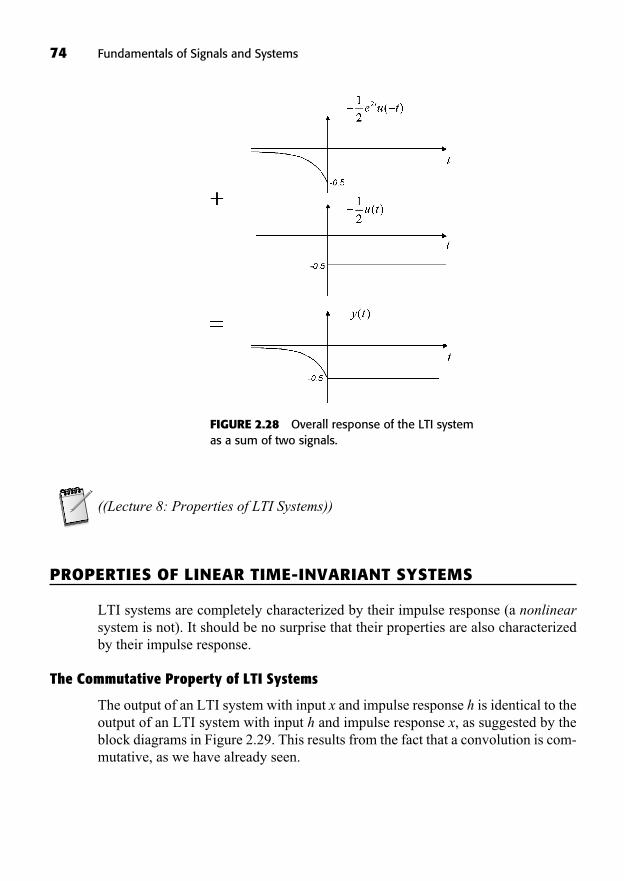
74 Fundamentals of Signals and Systems
((Lecture 8: Properties of LTI Systems))
PROPERTIES OF LINEAR TIME-INVARIANT SYSTEMS
LTI systems are completely characterized by their impulse response (a nonlinearsystem is not). It should be no surprise that their properties are also characterizedby their impulse response.
The Commutative Property of LTI Systems
The output of an LTI system with input x and impulse response h is identical to theoutput of an LTI system with input h and impulse response x, as suggested by theblock diagrams in Figure 2.29. This results from the fact that a convolution is com-mutative, as we have already seen.
FIGURE 2.28 Overall response of the LTI systemas a sum of two signals.

(2.33)
(2.34)y t x h t d h x t d( ) ( ) ( ) ( ) ( )= =+ +
y n x k h n k h k x n kk k
[ ] [ ] [ ] [ ] [ ]= == =
Linear Time-Invariant Systems 75
FIGURE 2.29 Equivalent block diagramsof LTI systems with respect to the output.
The Distributive Property of LTI Systems
The distributive property of LTI systems comes from the fact that a convolution isdistributive:
(2.35)
which means that summing the outputs of two systems subjected to the same inputis equivalent to a system with an impulse response equal to the sum of the impulseresponses of the two individual systems, as shown in Figure 2.30.
x h h x h x h+ = +( )1 2 1 2
FIGURE 2.30 System equivalent to aparallel interconnection of LTI systems.
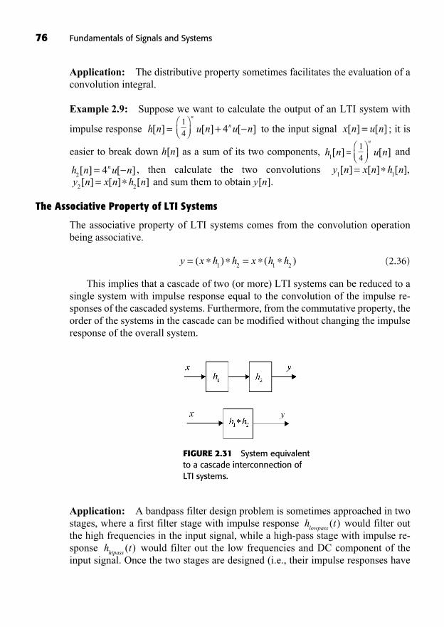
76 Fundamentals of Signals and Systems
Application: The distributive property sometimes facilitates the evaluation of aconvolution integral.
Example 2.9: Suppose we want to calculate the output of an LTI system with
impulse response to the input signal ; it is
easier to break down h[n] as a sum of its two components, and
, then calculate the two convolutions and sum them to obtain y[n].
The Associative Property of LTI Systems
The associative property of LTI systems comes from the convolution operationbeing associative.
(2.36)
This implies that a cascade of two (or more) LTI systems can be reduced to asingle system with impulse response equal to the convolution of the impulse re-sponses of the cascaded systems. Furthermore, from the commutative property, theorder of the systems in the cascade can be modified without changing the impulseresponse of the overall system.
y x h h x h h= =( ) ( )1 2 1 2
y n x n h n2 2[ ] [ ] [ ]=
y n x n h n1 1[ ] [ ] [ ],=h n u nn
24[ ] [ ]=
u n[ ]n
1
4h n
1[ ] =
x n u n[ ] [ ]=u n u nn[ ] [ ]+ 4n
1
4h n[ ] =
FIGURE 2.31 System equivalentto a cascade interconnection ofLTI systems.
Application: A bandpass filter design problem is sometimes approached in twostages, where a first filter stage with impulse response would filter outthe high frequencies in the input signal, while a high-pass stage with impulse re-sponse would filter out the low frequencies and DC component of theinput signal. Once the two stages are designed (i.e., their impulse responses have
h thipass
( )
h tlowpass
( )
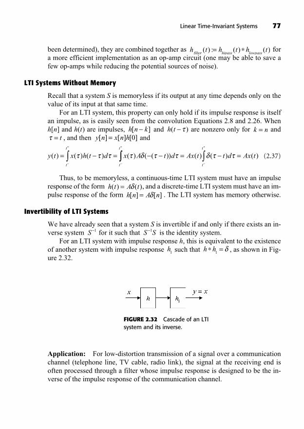
been determined), they are combined together as fora more efficient implementation as an op-amp circuit (one may be able to save afew op-amps while reducing the potential sources of noise).
LTI Systems Without Memory
Recall that a system S is memoryless if its output at any time depends only on thevalue of its input at that same time.
For an LTI system, this property can only hold if its impulse response is itselfan impulse, as is easily seen from the convolution Equations 2.8 and 2.26. Whenh[n] and h(t) are impulses, and are nonzero only for and
, and then and
(2.37)
Thus, to be memoryless, a continuous-time LTI system must have an impulseresponse of the form , and a discrete-time LTI system must have an im-pulse response of the form . The LTI system has memory otherwise.
Invertibility of LTI Systems
We have already seen that a system S is invertible if and only if there exists an in-verse system for it such that is the identity system.
For an LTI system with impulse response h, this is equivalent to the existenceof another system with impulse response such that , as shown in Fig-ure 2.32.
h h =1
h1
S S1S 1
h n A n[ ] [ ]=h t A t( ) ( )=
y t x h t d x A t dt
t
t
t
( ) ( ) ( ) ( ) ( ( ))= =+ +
= =+
Ax t t d Ax tt
t
( ) ( ) ( )
y n x n h[ ] [ ] [ ]= 0= tk n=h t( )h n k[ ]
h t h t h tfilter hipass lowpass
( ) : ( ) ( )=
Linear Time-Invariant Systems 77
FIGURE 2.32 Cascade of an LTIsystem and its inverse.
Application: For low-distortion transmission of a signal over a communicationchannel (telephone line, TV cable, radio link), the signal at the receiving end isoften processed through a filter whose impulse response is designed to be the in-verse of the impulse response of the communication channel.

Example 2.10: A system with impulse response delays its inputsignal by time T. Its inverse system is a time advance of T with impulse response
, as we now show. (Here we make use of the sampling property ofthe impulse function and we use the fact that .)
(2.38)
Causality of an LTI System
Recall that a system is causal if its output depends only on past and/or present val-ues of the input signal. Specifically, for a discrete-time LTI system, this require-ment is that y[n] should not depend on x[k] for k > n. Thus, looking back at theconvolution sum in Equation 2.8, the impulse response should satisfy for k > n, which is equivalent to for k < 0. Therefore, a discrete-time LTIsystem is causal if and only if its impulse response is zero for negative times. Thismakes sense, as a causal system should not exhibit a response before the impulseis applied at time n = 0.
A similar analysis for a continuous-time LTI system leads us to the same con-clusion. Namely, a continuous-time LTI system is causal if and only if
.
Example 2.11: A linear time-invariant circuit is causal. In fact, virtually all phys-ical systems are causal since it is impossible for them to predict the future.
BIBO Stability of LTI Systems
Recall that a system is BIBO stable if for every bounded input, the output is alsobounded. Let us consider a discrete-time system with impulse response h[n]. As-sume that the discrete-time signal x[n] is bounded by B for all n. Then, the magni-tude of the system’s output can be bounded using the triangle inequality as follows:
h t t( ) ,= <0 0
h k[ ] = 0h n k[ ] = 0
h t h t h h t d T t T( ) ( ) ( ) ( ) ( ) (= = ++
1 1))
( ) ( ( )) ( ) (
d
T t T d T
+
+
= =
= + = +
+
+
t T d
T t T d t
)
( ) ( ( )) ( TT T t T d
t
+
=
+
) ( ( ))
( )
( ) ( )t t=h t t T
1( ) ( )= +
h t t T( ) ( )=
78 Fundamentals of Signals and Systems
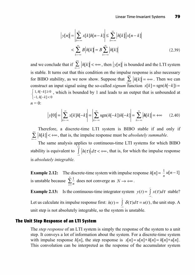
(2.39)
and we conclude that if , then is bounded and the LTI system
is stable. It turns out that this condition on the impulse response is also necessary
for BIBO stability, as we now show. Suppose that . Then we can
construct an input signal using the so-called signum function
, which is bounded by 1 and leads to an output that is unbounded at
n = 0:
(2.40)
Therefore, a discrete-time LTI system is BIBO stable if and only if , that is, the impulse response must be absolutely summable.
The same analysis applies to continuous-time LTI systems for which BIBO
stability is equivalent to , that is, for which the impulse response
is absolutely integrable.
Example 2.12: The discrete-time system with impulse response
is unstable because does not converge as .
Example 2.13: Is the continuous-time integrator system stable?
Let us calculate its impulse response first: , the unit step. A
unit step is not absolutely integrable, so the system is unstable.
The Unit Step Response of an LTI System
The step response of an LTI system is simply the response of the system to a unitstep. It conveys a lot of information about the system. For a discrete-time systemwith impulse response h[n], the step response is .This convolution can be interpreted as the response of the accumulator system
s n u n h n h n u n[ ] [ ] [ ] [ ] [ ]= =
d u t( ) ( )=t
h t( ) =
x d( )t
y t( ) =
N +1
1 nn
N
=
u n[ ]1n
1h n[ ] =
h d( ) < ++
h k[ ] < +k=
+
y x k h k h k h kk k
[ ] [ ] [ ] sgn( [ ]) [ ]0 = = == =
hh kk
[ ]=
= +
h k
h k
, [ ]
, [ ] <1 0
1 0
x k h k[ ] sgn( [ ])= =h k[ ] = +
k=
+
y n[ ]h k[ ] < +k=
+
y n x k h n k h k x n k
B h k
k k
[ ] [ ] [ ] [ ] [ ]
[
=
<
= =
]] [ ]k k
B h k= =
=
Linear Time-Invariant Systems 79
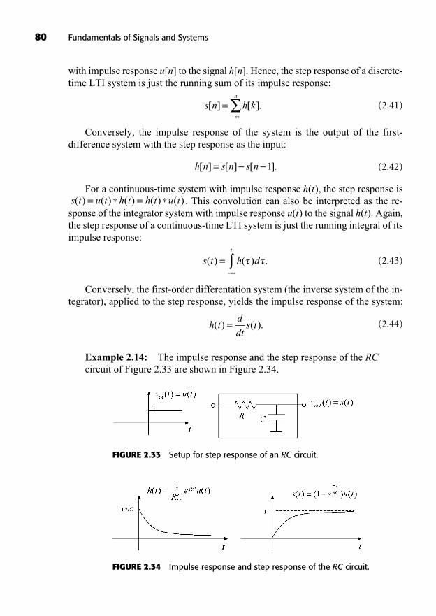
80 Fundamentals of Signals and Systems
with impulse response u[n] to the signal h[n]. Hence, the step response of a discrete-time LTI system is just the running sum of its impulse response:
(2.41)
Conversely, the impulse response of the system is the output of the first-difference system with the step response as the input:
(2.42)
For a continuous-time system with impulse response h(t), the step response is. This convolution can also be interpreted as the re-
sponse of the integrator system with impulse response u(t) to the signal h(t). Again,the step response of a continuous-time LTI system is just the running integral of itsimpulse response:
(2.43)
Conversely, the first-order differentation system (the inverse system of the in-tegrator), applied to the step response, yields the impulse response of the system:
(2.44)
Example 2.14: The impulse response and the step response of the RCcircuit of Figure 2.33 are shown in Figure 2.34.
h td
dts t( ) ( ).=
s t h dt
( ) ( ) .=
s t u t h t h t u t( ) ( ) ( ) ( ) ( )= =
h n s n s n[ ] [ ] [ ].= 1
s n h kn
[ ] [ ].=
FIGURE 2.33 Setup for step response of an RC circuit.
FIGURE 2.34 Impulse response and step response of the RC circuit.
SUMMARY
In this chapter, we have studied linear time-invariant systems.
An LTI system is completely characterized by its impulse response.The input-output relationship of an LTI discrete-time system is given by theconvolution sum of the system’s impulse response with the input signal.The input-output relationship of an LTI continuous-time system is given by theconvolution integral of the system’s impulse response with the input signal.Given the impulse response of an LTI system and a specific input signal, theconvolution giving the output signal can be computed using a graphical ap-proach or a numerical approach.The main properties of an LTI system were derived in terms of its impulseresponse.
TO PROBE FURTHER
For a more detailed presentation of linear time-invariant and time-varying systems,including multi-input multi-output systems, see Chen, 1999.
EXERCISES
Exercises with Solutions
Exercise 2.1
Compute the convolutions :(a) . Sketch the output signal y[n] for
the case , .
Answer:
y n x k h n k
u k u n k
k
k n k
k
[ ] [ ] [ ]
[ ] [ ]
=
=
=
+
=
++
=
= n
k
k
n
n0
0,
= 0 9.= 0 8.x n u n h n u nn n[ ] [ ], [ ] [ ],= =
y n x n h n[ ] [ ] [ ]=
Linear Time-Invariant Systems 81
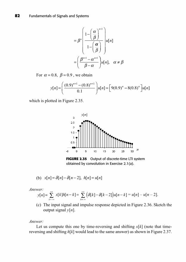
82 Fundamentals of Signals and Systems
For , we obtain
which is plotted in Figure 2.35.
y n u nn n
n[ ]( . ) ( . )
.[ ] ( . )= =
+ +0 9 0 80 1
9 0 91 1
8 0 8( . ) [ ]n u n
= =0 8 0 9. , .
+
= n
n 1
1
1
=+ +
u n
n n
[ ]
1 1
u n[ ],
FIGURE 2.35 Output of discrete-time LTI systemobtained by convolution in Exercise 2.1(a).
(b)
Answer:= u[n] – u[n – 2].
(c) The input signal and impulse response depicted in Figure 2.36. Sketch theoutput signal y[n].
Answer:Let us compute this one by time-reversing and shifting x[k] (note that time-
reversing and shifting h[k] would lead to the same answer) as shown in Figure 2.37.
k k u n k[ ] [ ] [ ]( )2k==
+x k h n k[ ] [ ] =
k=
+
y n[ ] =
x n n n h n u n[ ] [ ] [ ], [ ] [ ]= =2
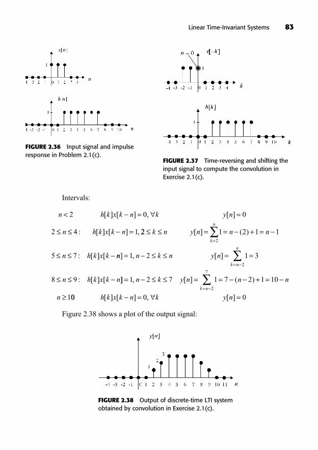
Intervals:
Figure 2.38 shows a plot of the output signal:
n h k x k n k y n
n h k x k n
< = =
=
2 0 0
2 4 1
[ ] [ ] , [ ]
: [ ] [ ] , 22 1 2 1 1
5 7
2
= = + ==
k n y n n n
n h k x k
k
n
[ ] ( )
: [ ] [ nn n k n y n
n h k x k n
k n
n
] , [ ]
: [ ] [
= = ==
1 2 1 3
8 9
2
]] , [ ] ( )= = = + ==
1 2 7 1 7 2 1 10
12
7
n k y n n n
nk n
00 0 0h k x k n k y n[ ] [ ] , [ ]= =
Linear Time-Invariant Systems 83
FIGURE 2.36 Input signal and impulseresponse in Problem 2.1(c).
FIGURE 2.37 Time-reversing and shifting theinput signal to compute the convolution inExercise 2.1(c).
FIGURE 2.38 Output of discrete-time LTI systemobtained by convolution in Exercise 2.1(c).
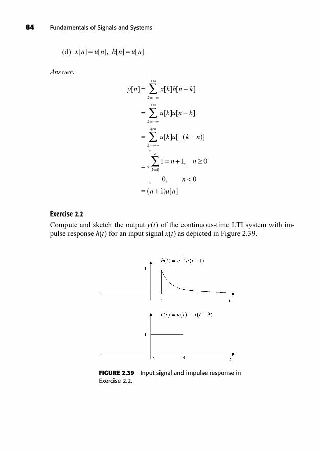
84 Fundamentals of Signals and Systems
(d)
Answer:
Exercise 2.2
Compute and sketch the output y(t) of the continuous-time LTI system with im-pulse response h(t) for an input signal x(t) as depicted in Figure 2.39.
y n x k h n k
u k u n k
u
k
k
[ ] [ ] [ ]
[ ] [ ]
[
=
=
=
=
+
=
+
kk u k n
n n
n
k
k
n
] [ ( )]
,
,
== +
<
=
+
=
1 1 0
0 00
= +( ) [ ]n u n1
x n u n h n u n[ ] [ ], [ ] [ ]= =
FIGURE 2.39 Input signal and impulse response inExercise 2.2.
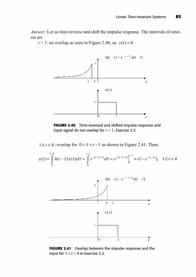
Answer: Let us time-reverse and shift the impulse response. The intervals of inter-est are
t < 1: no overlap as seen in Figure 2.40, so .y t( ) = 0
Linear Time-Invariant Systems 85
FIGURE 2.40 Time-reversed and shifted impulse response andinput signal do not overlap for t < 1, Exercise 2.2.
: overlap for as shown in Figure 2.41. Then,
y t h t x d e d et
tt
( ) ( ) ( ) ( ) (= = =0
11
0
1tt
tte t= <1
0
111 1 4) ( )( ),
0 1< < t1 4<t
FIGURE 2.41 Overlap between the impulse response and theinput for 1 t < 4 in Exercise 2.2.
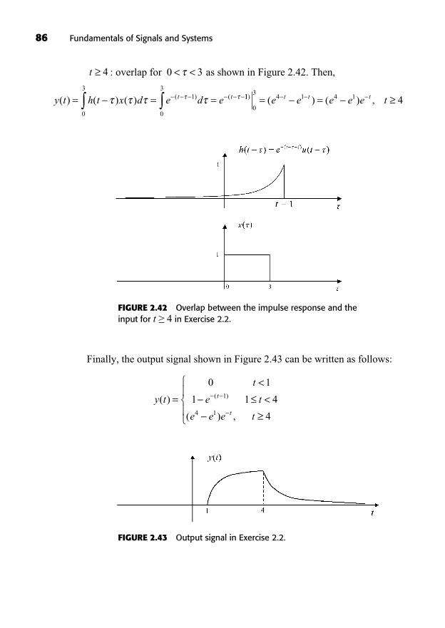
86 Fundamentals of Signals and Systems
: overlap for as shown in Figure 2.42. Then,
y t h t x d e d et t( ) ( ) ( ) ( ) (= = =0
31
0
311
0
34 1 4 1 4) ( ) ( ) ,= =e e e e e tt t t
0 3< <t 4
FIGURE 2.42 Overlap between the impulse response and theinput for t ≥ 4 in Exercise 2.2.
FIGURE 2.43 Output signal in Exercise 2.2.
Finally, the output signal shown in Figure 2.43 can be written as follows:
y t
t
e t
e e e t
t
t
( )
( ) ,
( )=<<
0 1
1 1 4
4
1
4 1
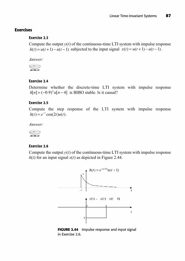
Exercises
Exercise 2.3
Compute the output y(t) of the continuous-time LTI system with impulse responsesubjected to the input signal .
Answer:
Exercise 2.4
Determine whether the discrete-time LTI system with impulse responseis BIBO stable. Is it causal?
Exercise 2.5
Compute the step response of the LTI system with impulse response.
Answer:
Exercise 2.6
Compute the output y(t) of the continuous-time LTI system with impulse responseh(t) for an input signal x(t) as depicted in Figure 2.44.
h t e t u tt( ) cos( ) ( )= 2
h n u nn[ ] ( . ) [ ]= 0 9 4
x t u t u t( ) ( ) ( )= +1 1h t u t u t( ) ( ) ( )= +1 1
Linear Time-Invariant Systems 87
FIGURE 2.44 Impulse response and input signalin Exercise 2.6.
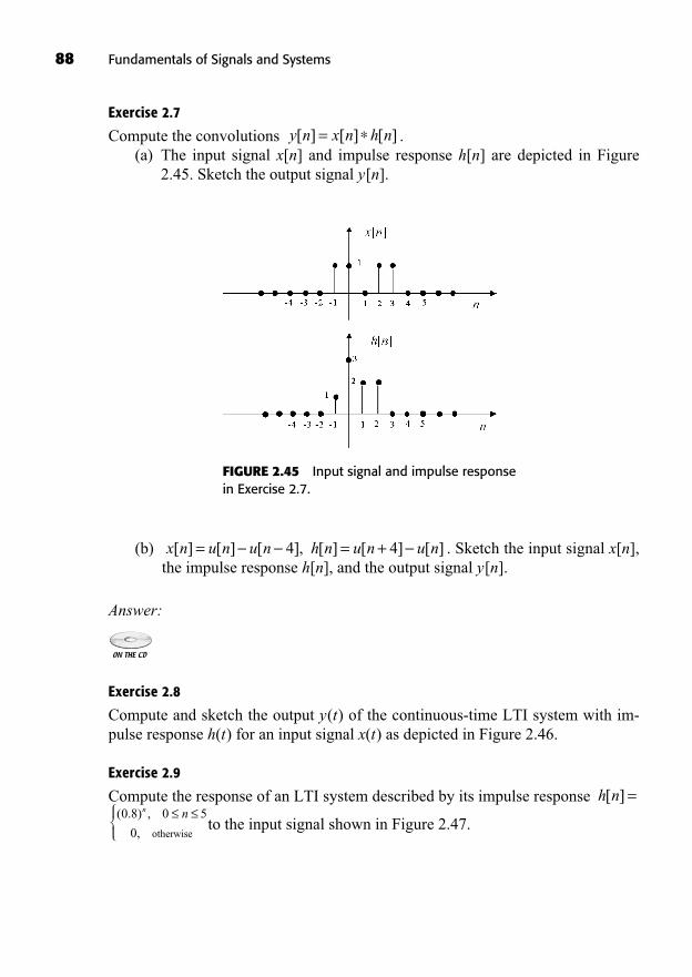
88 Fundamentals of Signals and Systems
Exercise 2.7
Compute the convolutions .(a) The input signal x[n] and impulse response h[n] are depicted in Figure
2.45. Sketch the output signal y[n].
y n x n h n[ ] [ ] [ ]=
FIGURE 2.45 Input signal and impulse responsein Exercise 2.7.
(b) . Sketch the input signal x[n],the impulse response h[n], and the output signal y[n].
Answer:
Exercise 2.8
Compute and sketch the output y(t) of the continuous-time LTI system with im-pulse response h(t) for an input signal x(t) as depicted in Figure 2.46.
Exercise 2.9
Compute the response of an LTI system described by its impulse response
to the input signal shown in Figure 2.47.nn( . ) ,
,
0 8 0 5
0 otherwise
h n[ ] =
x n u n u n h n u n u n[ ] [ ] [ ], [ ] [ ] [ ]= = +4 4
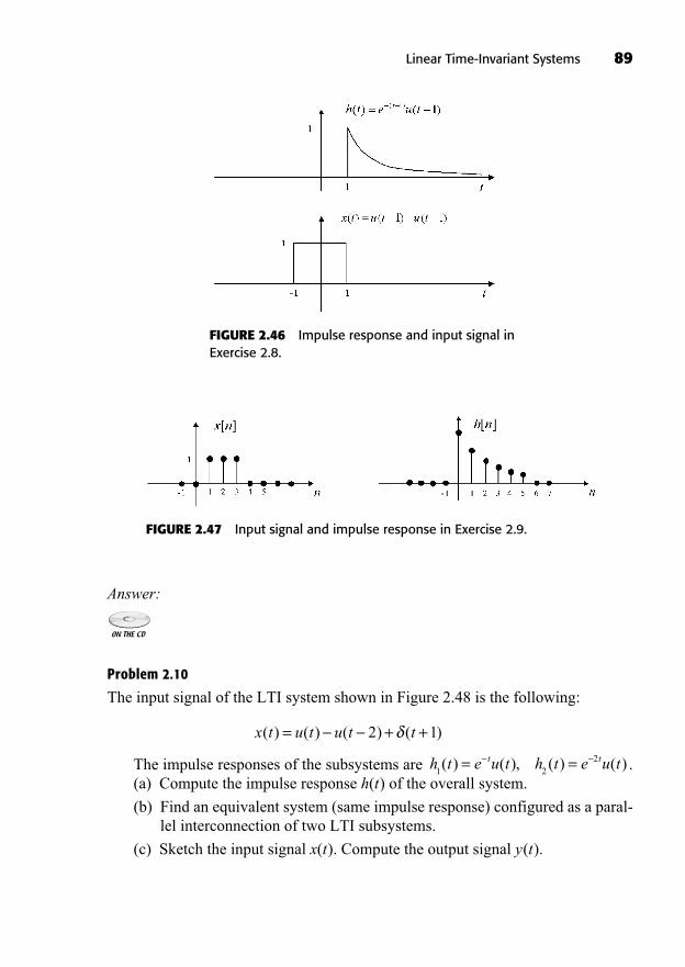
Answer:
Problem 2.10
The input signal of the LTI system shown in Figure 2.48 is the following:
The impulse responses of the subsystems are .(a) Compute the impulse response h(t) of the overall system.
(b) Find an equivalent system (same impulse response) configured as a paral-lel interconnection of two LTI subsystems.
(c) Sketch the input signal x(t). Compute the output signal y(t).
h t e u t h t e u tt t1 2
2( ) ( ), ( ) ( )= =
x t u t u t t( ) ( ) ( ) ( )= + +2 1
Linear Time-Invariant Systems 89
FIGURE 2.46 Impulse response and input signal inExercise 2.8.
FIGURE 2.47 Input signal and impulse response in Exercise 2.9.
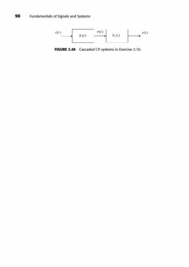
90 Fundamentals of Signals and Systems
FIGURE 2.48 Cascaded LTI systems in Exercise 2.10.
91
Differential and DifferenceLTI Systems
3
In This Chapter
Causal LTI Systems Described by Differential EquationsCausal LTI Systems Described by Difference EquationsImpulse Response of a Differential LTI SystemImpulse Response of a Difference LTI SystemCharacteristic Polynomials and Stability of Differential and Difference SystemsTime Constant and Natural Frequency of a First-Order LTI Differential SystemEigenfunctions of LTI Difference and Differential SystemsSummaryTo Probe FurtherExercises
((Lecture 9: Definition of Differential and Difference Systems))
Differential and difference linear time-invariant (LTI) systems constitute anextremely important class of systems in engineering. They are used in cir-cuit analysis, filter design, controller design, process modeling, and in
many other applications. We will review the classical solution approach for suchsystems. Figure 3.1 shows that differential systems form a subset of the set of con-tinuous-time LTI systems. A consequence of this set diagram is that any differen-tial system has an impulse response. The same is true for difference systems. Wewill show techniques to compute their impulse response.
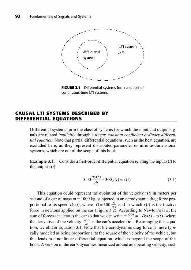
92 Fundamentals of Signals and Systems
CAUSAL LTI SYSTEMS DESCRIBED BY DIFFERENTIAL EQUATIONS
Differential systems form the class of systems for which the input and output sig-nals are related implicitly through a linear, constant coefficient ordinary differen-tial equation. Note that partial differential equations, such as the heat equation, areexcluded here, as they represent distributed-parameter or infinite-dimensionalsystems, which are out of the scope of this book.
Example 3.1: Consider a first-order differential equation relating the input x(t) tothe output y(t):
(3.1)
This equation could represent the evolution of the velocity y(t) in meters persecond of a car of mass m = 1000 kg, subjected to an aerodynamic drag force pro-portional to its speed Dy(t), where and in which x(t) is the tractiveforce in newtons applied on the car (Figure 3.2). According to Newton’s law, thesum of forces accelerates the car so that we can write m , wherethe derivative of the velocity is the car’s acceleration. Rearranging this equa-tion, we obtain Equation 3.1. Note that the aerodynamic drag force is more typi-cally modeled as being proportional to the square of the velocity of the vehicle, butthis leads to a nonlinear differential equation, which is beyond the scope of thisbook. A version of the car’s dynamics linearized around an operating velocity, such
dy t
dt
( )Dy t x t( ) ( )= − +dy t
dt
( )
N
m/sD = 300
1000 300dy t
dty t x t
( )( ) ( )+ =
FIGURE 3.1 Differential systems form a subset ofcontinuous-time LTI systems.
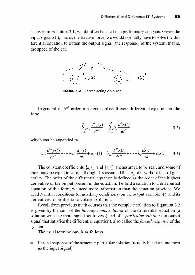
as given in Equation 3.1, would often be used in a preliminary analysis. Given theinput signal x(t), that is, the tractive force, we would normally have to solve the dif-ferential equation to obtain the output signal (the response) of the system, that is,the speed of the car.
Differential and Difference LTI Systems 93
FIGURE 3.2 Forces acting on a car.
In general, an Nth-order linear constant coefficient differential equation has theform
(3.2)
which can be expanded to
(3.3)
The constant coefficients and are assumed to be real, and some ofthem may be equal to zero, although it is assumed that without loss of gen-erality. The order of the differential equation is defined as the order of the highestderivative of the output present in the equation. To find a solution to a differentialequation of this form, we need more information than the equation provides. Weneed N initial conditions (or auxiliary conditions) on the output variable y(t) and itsderivatives to be able to calculate a solution.
Recall from previous math courses that the complete solution to Equation 3.2is given by the sum of the homogeneous solution of the differential equation (asolution with the input signal set to zero) and of a particular solution (an outputsignal that satisfies the differential equation), also called the forced response of thesystem.
The usual terminology is as follows:
Forced response of the system = particular solution (usually has the same formas the input signal)
aN≠ 0
bi i
M{ } =1a
i i
N{ } =1
ad y t
dta
dy t
dta y t b
d x t
dtN
N
N M
M
M
( ) ( )( )
( )+ + + = +�
1 0��+ +b
dx t
dtb x t
1 0
( )( ).
ad y t
dtb
d x t
dtk
k
kk
N
k
k
kk
M( ) ( )
= =∑ ∑=
0 0
94 Fundamentals of Signals and Systems
Natural response of the system = homogeneous solution (depends on initialconditions and forced response)
A few authors use the term forced response as meaning the system’s responseto the input with zero initial conditions. However, in this book, and in most of therelevant literature, such a response is called a zero-state response (more on thislater.)
Example 3.2: Consider the LTI system described by the causal linear constantcoefficient differential Equation 3.1. We will calculate the output of this system,that is, the car velocity, from a standstill, to the input tractive force signal
. This input signal could correspond to the driver stepping on the gas pedal from a standstill and then rapidly easing the throttle. As statedabove, the solution is composed of a homogeneous response (natural response) anda particular solution (forced response) of the system:
(3.4)
where the particular solution satisfies Equation 3.1, and the homogeneous solutionyh(t) satisfies
(3.5)
Step 1: For the particular solution for t > 0, we consider a signal yp(t) of thesame form as x(t) for t > 0: , where coefficient is to be de-termined. Substituting the exponentials for x(t) and yp(t) in Equation 3.1, weget
(3.6)
which simplifies to and yields .Thus, we have
(3.7)
Remark: The particular solution seems to indicate a negative velocity, that is,the car moving backward, which would not make sense, but the full solution needsto be considered, not just the particular solution.
y t e tp
t( ) . , .= − >−2 941 02
= −2 941.50001700C = −− + =2000 300 5000C C
− + =− − −2000 300 50002 2 2Ce Ce et t t ,
C ∈Ry t Cep
t( ) = −2
1000 300 0dy t
dty th
h
( )( ) .+ =
y t y t y th p
( ) ( ) ( ),= +
x t e u tt( ) ( )= −5000 2 N
Step 2: Now we want to determine yh(t), the natural response of the system.We assume a solution of the form of an exponential: yh(t) = Aest, where A ≠ 0 .Substituting this exponential into Equation 3.5, we get
(3.8)
which simplifies to . This equation holds for . Also, withthis value for s, is a solution to the homogeneous Equation 3.5 for anychoice of A.
Combining the natural response and the forced response, we find the solutionto the differential Equation 3.1:
(3.9)
Now, because we have not yet specified an initial condition on y(t), this re-sponse is not completely determined, as the value of A is still unknown.
Strictly speaking, for causal LTI systems defined by linear constant-coefficientdifferential equations, the initial conditions must be ,what is called initial rest. That is, if at least one initial condition is nonzero, thenstrictly speaking, the system is nonlinear. In practice, we often encounter nonzeroinitial conditions and still refer to the system as being linear.
In Example 3.2, initial rest implies that y(0) = 0, so that
(3.10)
and we get A = 2.941. Thus, for t > 0, the car velocity is given by
(3.11)
What about the negative times t < 0? The condition of initial rest and thecausality of the system imply that since . Therefore,we can write the speed of the car as follows:
(3.12)
This speed signal is plotted in Figure 3.3, and we can see that the car is mov-ing forward, as expected.
y t e e u tt t( ) . ( ) ( )..= −− −2 941 0 3 2
∀ ∈t Rx t t( ) ,= <0 0y t t( ) ,= <0 0
y t e e tt t( ) . ( ), ..= − >− −2 941 00 3 2
y A( ) . ,0 2 941 0= − =
0=d y
dt
N
N
( )01
1
−
−= =�dy
dt
( )0y( )0 =
y t y t y t Ae e th p
t t( ) ( ) ( ) . , ..= + = − >− −0 3 22 941 0
Ae t−0 3.s = −0 3.s + =0 3 0.
0 1000 300 1000 300= + = +Ase Ae A s est st st( ) ,
Differential and Difference LTI Systems 95
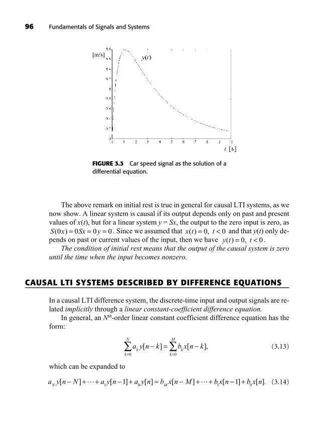
96 Fundamentals of Signals and Systems
The above remark on initial rest is true in general for causal LTI systems, as wenow show. A linear system is causal if its output depends only on past and presentvalues of x(t), but for a linear system y = Sx, the output to the zero input is zero, as
. Since we assumed that and that y(t) only de-pends on past or current values of the input, then we have .
The condition of initial rest means that the output of the causal system is zerountil the time when the input becomes nonzero.
CAUSAL LTI SYSTEMS DESCRIBED BY DIFFERENCE EQUATIONS
In a causal LTI difference system, the discrete-time input and output signals are re-lated implicitly through a linear constant-coefficient difference equation.
In general, an Nth-order linear constant coefficient difference equation has theform:
(3.13)
which can be expanded to
(3.14)a y n N a y n a y n b x n M b x nN M
[ ] [ ] [ ] [ ] [− + + − + = − + +� �1 0 1
1 −− +10
] [ ].b x n
a y n k b x n kk
k
N
kk
M
[ ] [ ],− = −= =∑ ∑
0 0
y t t( ) ,= <0 0x t t( ) ,= <0 0S x Sx y( )0 0 0 0= = =
FIGURE 3.3 Car speed signal as the solution of adifferential equation.
The constant coefficients and are assumed to be real, and althoughsome of them may be equal to zero, it is assumed that without loss of gen-erality. The order of the difference equation is defined as the longest time delay ofthe output present in the equation. To find a solution to the difference equation, weneed more information than what the equation provides. We need N initial condi-tions (or auxiliary conditions) on the output variable (its N past values) to be ableto compute a specific solution.
General Solution
A general solution to Equation 3.13 can be expressed as the sum of a homogeneous
solution (natural response) to and a particular solution (forced
response), in a manner analogous to the continuous-time case.
(3.15)
The concept of initial rest of the LTI causal system described by the differenceequation here means that implies .
Example 3.3: Consider the first-order difference equation initially at rest:
(3.16)
The solution is composed of a homogeneous response (natural response), anda particular solution (forced response) of the system:
(3.17)
where the particular solution satisfies Equation 3.16 for n ≥ 0, and the homoge-neous solution satisfies
(3.18)
For the particular solution for n ≥ 0, we look for a signal yp[n] of the same formas x[n]: . Then, we get
(3.19)
Y Y
Y
n n n( . ) . ( . ) ( . )
. ( . )
− + − = −⇔
+ −
−0 8 0 5 0 8 0 8
1 0 5 0 8
1
−−⎡⎣
⎤⎦ =
=
1 1
83
Y ,
y n Ypn[ ] ( . )= −0 8
y n y nh h[ ] . [ ] .+ − =0 5 1 0
y n y n y nh p[ ] [ ] [ ],= +
y n y n u nn[ ] . [ ] ( . ) [ ].+ − = −0 5 1 0 8
y n n n[ ] ,= ∀ <00
x n n n[ ] ,= ∀ <00
y n y n y nh p
[ ] [ ] [ ].= +
a y n kk
[ ]− =∑ 0k
N
=∑
0
aN≠ 0
bi i
M{ } =1a
i i
N{ } =1
Differential and Difference LTI Systems 97
which yields
(3.20)
Now let us determine yh[n], the natural response of the system. We hypothesizea solution of the form of an exponential signal: . Substituting this ex-ponential in Equation 3.18, we get
(3.21)
With this value for z, is a solution to the homogeneous equa-tion for any choice of A. Combining the natural response and the forced response,we find the solution to the difference Equation 3.16 for n ≥ 0:
(3.22)
The assumption of initial rest implies y [–1] = 0, but we need to use an initialcondition at a time where the forced response exists ( for n ≥ 0), that is, y[0], whichcan be obtained by a simple recursion.
(3.23)
Note that this remark also holds for higher-order systems. For instance, the re-sponse of a second-order system initially at rest satisfies the conditions y [–2] =y[–1] = 0, but y[0], y[1] must be computed recursively and used as new initial con-ditions in order to obtain the correct coefficients in the homogeneous response. Inour example, the coefficient is computed as follows:
(3.24)
y A A
A
[ ] ( . ) ( . )0 1 0 583
0 883
53
0 0= = − + − = +
⇒ = −
y n y n u n
n y y
n[ ] . [ ] ( . ) [ ]
: [ ] . [
= − − + −
= = − −
0 5 1 0 8
0 0 0 5 11 0 8 0 1 10] ( . )+ − = + =
y n y n y n Ah pn n[ ] [ ] [ ] ( . ) ( . ) .= + = − + −0 5
83
0 8
y n Ahn[ ] ( . )= −0 5
Az Az
z
z
n n+ =⇔+ == −
−
−
0 5 0
1 0 5 0
0 5
1
1
.
.
. .
y n Azhn[ ] =
y npn[ ] ( . ) .= −8
30 8
98 Fundamentals of Signals and Systems
Therefore, the complete solution is (check that it satisfies Equation 3.16 as anexercise)
(3.25)
Recursive Solution
In the discrete-time case, we have an alternative to compute y[n]: we can computeit recursively using Equation 3.13 rearranged so that all the terms are brought to theright-hand side, except y[n]:
(3.26)
Suppose that the system is initially at rest and that x[n] has nonzero valuesstarting at n = 0. Then, the condition of initial rest means that y [–1] = y[–2] = . . .
= y[–N] = 0, and one can start computing y[n] recursively. This is often how digi-tal filters are implemented on a computer or a digital signal processor board. Thisis also how a simulation of the response of a differential equation is typically com-puted: first, the differential equation is discretized at a given sampling rate to ob-tain a difference equation, and then the response of the difference equation iscomputed recursively. We will talk about sampling and system discretization insome detail in subsequent chapters.
Example 3.4: Consider the difference equation:
(3.27)
Taking the second and third terms on the left-hand side of Equation 3.27 to theright-hand side, we obtain the recursive form of the difference equation:
(3.28)
Assuming initial rest and that the input is an impulse , we have, and the recursion can be started:y y[ ] [ ]− = − =2 1 0
x n n[ ] [ ]= δ
y n y n y n x n x n[ ] [ ] [ ] [ ] [ ].= − − − + − −5
61
1
62 3 2 1
y n y n y n x n x n[ ] [ ] [ ] [ ] [ ].− − + − = − −5
61
1
62 3 2 1
y na
b x n k a y n kk
k
M
kk
N
[ ] [ ] [ ] .= − − −⎛⎝⎜
⎞⎠⎟= =
∑ ∑1
0 0 1
y n u n u nn n[ ] ( . ) [ ] ( . ) [ ].= − − + −53
0 583
0 8
Differential and Difference LTI Systems 99
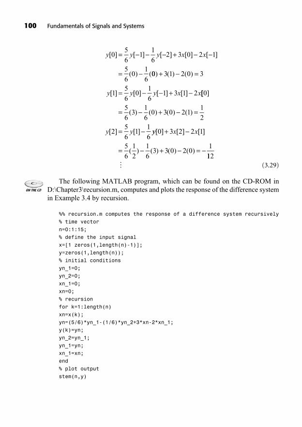
100 Fundamentals of Signals and Systems
(3.29)
The following MATLAB program, which can be found on the CD-ROM inD:\Chapter3\recursion.m, computes and plots the response of the difference systemin Example 3.4 by recursion.
%% recursion.m computes the response of a difference system recursively
% time vector
n=0:1:15;
% define the input signal
x=[1 zeros(1,length(n)-1)];
y=zeros(1,length(n));
% initial conditions
yn_1=0;
yn_2=0;
xn_1=0;
xn=0;
% recursion
for k=1:length(n)
xn=x(k);
yn=(5/6)*yn_1-(1/6)*yn_2+3*xn-2*xn_1;
y(k)=yn;
yn_2=yn_1;
yn_1=yn;
xn_1=xn;
end
% plot output
stem(n,y)
y y y x x[ ] [ ] [ ] [ ] [ ]
( ) (
05
61
1
62 3 0 2 1
5
60
1
6
= − − − + − −
= − 00 3 1 2 0 3
15
60
1
61 3 1 2
) ( ) ( )
[ ] [ ] [ ] [ ]
+ − =
= − − + −y y y x x[[ ]
( ) ( ) ( ) ( )
[ ] [ ]
0
5
63
1
60 3 0 2 1
1
2
25
61
1
6
= − + − =
= −y y yy x x[ ] [ ] [ ]
( ) ( ) ( ) ( )
0 3 2 2 1
5
6
1
2
1
63 3 0 2 0
1
+ −
= − + − = −112
�

Note that because this system is LTI, it is completely determined by its impulseresponse. Thus, the response to the unit impulse that we obtain here numerically byrecursion is actually the impulse response of the system. For a simpler first-ordersystem, it is often easy to find the “general term” describing the impulse responseh[n] for any time step n. For example, you can check that the causal LTI system de-scribed by the difference equation,
(3.30)
has an impulse response given by .
((Lecture 10: Impulse Response of a Differential System))
IMPULSE RESPONSE OF A DIFFERENTIAL LTI SYSTEM
Consider again the general form of a causal LTI differential system of order N:
(3.31)
In this section, we give two methods to compute the impulse response of sucha system.
Method 1: Impulse Response Obtained by Linear Combination of ImpulseResponses of the Left-Hand Side of the Differential Equation
The step-by-step procedure to find the impulse response of a differential LTI sys-tem is as follows:
1. Replace the whole right-hand side of the differential Equation 3.31 by δ(t).2. Integrate this new equation from t = 0– to t = 0+ to find a set of initial con-
ditions at t = 0.3. Calculate the homogeneous response ha(t) to the homogeneous equation
with these initial conditions.4. Finally, differentiate the homogeneous response ha(t) and use linear super-
position according to the right-hand side of the differential equation toform the overall response of the system.
The procedure is based on the properties of linearity and commutativity of LTIsystems. Differential systems can be seen as the combination of two subsystems,
ad y t
dtb
d x t
dtk
k
kk
N
k
k
kk
M( ) ( ).
= =∑ ∑=
0 0
h n u nn
[ ] [ ]= −( )2
y n y n x n[ ] [ ] [ ],+ − =2 1
Differential and Difference LTI Systems 101

102 Fundamentals of Signals and Systems
each one defined by a side of the differential equation, as illustrated in Figure 3.4.The first subsystem processes the input signal by implementing the right-hand sideof the equation, that is, by forming a linear combination of the input and its deriv-atives. The second subsystem implements the left-hand side of the differentialequation, with its input being the output of the first subsystem. Both of these sub-systems are LTI, and therefore each one has an impulse response. Let the impulseresponse of the second one be denoted as ha(t). Another consequence of the LTIproperties is that, by commutativity, the order of the subsystems can be inter-changed, as shown in Figure 3.5.
FIGURE 3.4 Differential system as the cascade of two LTI subsystems.
The block diagram in Figure 3.5 suggests how the procedure works. Steps 1–3compute the impulse response ha(t) of the first block, and Step 4 computes the im-pulse response of the overall differential system by applying the second block (theright-hand side of the differential equation) to ha(t) in order to get h(t).
Step 1: Under the assumption that and the system is initially at rest,that is,
ydy
dt
d y
dt
N
N( )
( ) ( ),0
0 00
1
1
−− − −
−= = = =�
N M≥
FIGURE 3.5 Cascade of two LTI subsystems equivalent to the differential system.
we first replace the right-hand side of Equation 3.31 with a single unit impulse:
(3.32)
Step 2: To solve this equation for ha(t), we first observe that the impulse canonly be generated by the highest-order derivative (i.e., k = N) of ha(t). Other-wise, we would have derivatives of the impulse function in the right-hand side
of Equation 3.5. This means that the functions aresmooth or have finite discontinuities at worst. Such functions integrated overan infinitesimally small interval simply vanish. This important observation(make sure you understand it!) gives us the first N – 1 initial conditions for ha(t)when we integrate those functions from t = 0– to t = 0+:
(3.33)
Then, integrating both sides of Equation 3.32 from t = 0– to t = 0+, we obtain
(3.34)
which gives us our Nth initial condition at t = 0+:
(3.35)
Step 3: Thus, starting at time t = 0+, we need to solve the homogeneousequation,
(3.36)
subject to the above initial conditions. Assume that the solution has the form ofa complex exponential Aest for t > 0, where . Substituting this expo-nential into Equation 3.36, we get a polynomial in s multiplying an exponen-tial on the left-hand side:
(3.37)Ae a sstk
k
k
N
=∑ =
0
0.
A s, ∈C
ad h t
dtk
kak
k
N ( ),
=∑ =
0
0
d h
dt a
Na
NN
− +
− =1
1
0 1( ).
ad h
dtd a
d h
dtd a
d h
dk
ka
k N
NaN N
Na
( ) ( ) ( )ττ
ττ= =
− +1 0
tt Nk
N
−= −
+
−
+
∫∫∑ =1
0
0
0
0
0
1,
d h
dtd
d h
dtk N
ka
k
kak
( ) ( ), , ,
ττ
0
0 1
1
00 1
−
+
∫ = = =− +
− … −−1.
d h t
dt
Na
N
( )−
−
1
1, ,�dh t
dta( )
h ta( ),
ad h t
dtt
k
kak
k
N ( )( ).
=∑ =
0
δ
Differential and Difference LTI Systems 103
With the assumption that A ≠ 0, this equation holds if and only if the charac-
teristic polynomial vanishes at the complex number s:
(3.38)
By the fundamental theorem of algebra, Equation 3.38 has at most N distinctcomplex roots. Assume for simplicity that the N roots are distinct, and let them bedenoted as . This means that there are N distinct functions that satisfythe homogeneous Equation 3.36. Then, the solution to Equation 3.36 can be writ-ten as a linear combination of these complex exponentials:
(3.39)
The N complex coefficients can be computed using the initial conditions:
(3.40)
This set of linear equations can be written as follows:
(3.41)
The N � N matrix with complex entries in this equation is called a Vander-monde matrix and it can be shown to be nonsingular (invertible). Thus, a uniquesolution always exists for the Ak’s, which gives us the unique solution ha(t) throughEquation 3.39.
0
0
0
1
1 1 1
1 2
12
22
�
��
�
a
s s s
s s s
N
N
⎡
⎣
⎢⎢⎢⎢⎢⎢
⎤
⎦
⎥⎥⎥⎥⎥⎥
= NN
N NN
Ns s s
A
A
A
A
2
1 2
1
2
3
� � � �
�
�
⎡
⎣
⎢⎢⎢⎢⎢⎢⎢
⎤
⎦
⎥⎥⎥⎥⎥⎥⎥ NN
⎡
⎣
⎢⎢⎢⎢⎢⎢⎢
⎤
⎦
⎥⎥⎥⎥⎥⎥⎥
.
0 0
00
0
1 1
= = =
= =
+
= =+
+∑ ∑h A e A
dh
dtA
a k
s
k
N
kk
N
ak
k( )
( )ss
a
d h
dtA s
kk
N
N
Na
N k kN
k
N
=
− +
−−
=
∑
∑= =
1
1
1
1
1
1 0
�
( ).
Ak k
N{ } =1
h t A ea k
s t
k
Nk( ) .=
=∑
1
A ek
s tksk k
N{ } =1
p s a s a s a s ak
k
k
N
NN
NN( ) .= = + + + =
=−
−∑0
11
00�
a sk
k∑0k
N
=∑
0
p s( ) :=
104 Fundamentals of Signals and Systems
Step 4: Finally, the impulse response of the general causal LTI system describedby Equation 3.31 is a linear combination of ha(t) and its derivatives as shown inthe second block of Figure 3.4. Hence, the impulse response is given by
(3.42)
Example 3.5: Consider the first-order system initially at rest with time constant τ0 > 0:
(3.43)
Step 1: Set up the first problem of calculating the impulse response of the left-hand side of the differential equation.
(3.44)
Step 2: Find the initial condition of the homogeneous equation at t = 0+ byintegrating on both sides of Equation 3.2 from t = 0– to t = 0+. Note that the im-pulse is produced by the term , so ha(t) will have a finite jump at most.Thus we have
(3.45)
and hence is our initial condition for the homogeneous equation:
(3.46)
Step 3: The characteristic polynomial is and it has one zero at s = –τ0
–1 which means that the homogeneous response has the form
for t > 0. The initial condition allows us to determine the con-stant A:
(3.47)h Aa( ) ,0
1
0
+ = =τ
h t Aea
t
( ) =−τ0
p s s( ) = +τ0
1
τ0
0dh t
dth ta
a
( )( ) .+ =
1
0τ
ha( )0+ =
ττ
τ τ τ τ0
0
0
0
0
0
0
dh
dtd h d ha
a a
( )( ) (
−
+
−
+
∫ ∫+ =
=� �� ��
00 1+ =) ,
dh t
dta( )τ
0
τ δ0
dh t
dth t ta
a
( )( ) ( )+ =
τ0
dy t
dty t
d
dtx t x t
( )( ) ( ) ( ).+ = +
h t bd h t
dtk
kak
k
M
( )( )
.==∑
0
Differential and Difference LTI Systems 105
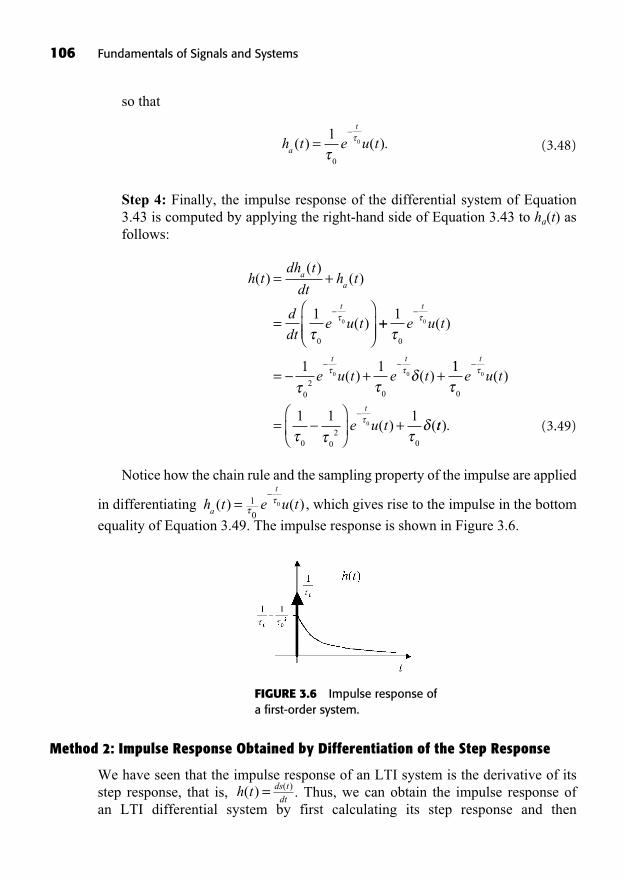
106 Fundamentals of Signals and Systems
so that
(3.48)
Step 4: Finally, the impulse response of the differential system of Equation3.43 is computed by applying the right-hand side of Equation 3.43 to ha(t) asfollows:
(3.49)
Notice how the chain rule and the sampling property of the impulse are applied
in differentiating , which gives rise to the impulse in the bottom
equality of Equation 3.49. The impulse response is shown in Figure 3.6.
h t e u ta
t
( ) ( )=−
1
00
ττ
h tdh t
dth t
d
dte u t
aa
t
( )( )
( )
( )
= +
=⎛
⎝⎜⎜
⎞
⎠⎟⎟
−1
0
0
ττ ++
= − + +
−
− −
1
1 1
0
02
0
0
0 0
τ
τ τδ
τ
τ τ
e u t
e u t e t
t
t t
( )
( ) ( )11
1 1 1
0
0 02
0
0
0
τ
τ τ τδ
τ
τ
e u t
e u t
t
t
−
−= −⎛
⎝⎜
⎞
⎠⎟ +
( )
( ) (tt).
h t e u ta
t
( ) ( ).=−1
0
0
ττ
FIGURE 3.6 Impulse response ofa first-order system.
Method 2: Impulse Response Obtained by Differentiation of the Step Response
We have seen that the impulse response of an LTI system is the derivative of itsstep response, that is, . Thus, we can obtain the impulse response of an LTI differential system by first calculating its step response and then
ds tdt( )h t( ) =
differentiating it. This method is useful when the right-hand side of the differentialequation does not have derivatives of the input signal.
Example 3.6: We will illustrate this technique with an example of a second-order system. Consider the following causal LTI differential system initially atrest:
(3.50)
Let x(t) = u(t). The characteristic polynomial of this system is
(3.51)
and its zeros (values of s for which p(s) = 0) are s = –2 and s = –1. Hence, thehomogeneous solution has the form
(3.52)
We look for a particular solution of the form yp(t) = K for t > 0 when x(t) = 1.Substituting in Equation 3.50, we find
(3.53)
By adding the homogeneous and particular solutions, we obtain the overall stepresponse for t > 0:
(3.54)
The initial conditions at t = 0– are . Because the input sig-
nal has a finite jump at t = 0+, it will be included in only, and will
be continuous. Hence, , and we have
(3.55)
y A A
dy
dtA A
( )
( ).
01
20
02 0
1 2
1 2
+
+
= + + =
= − − =
0=dy
dt
( )0+
=dy
dt
( )0−
y t, ( )dy t
dt
( )d y t
dt
2
2
( )y, ( )0 0 0−= =dy
dt
( )0−
s t A e A et t( ) .= + +− −1
22
1
2
y tp( ) .=
1
2
y t A e A eh
t t( ) .= +− −1
22
p s s s s s( ) ( )( ),= + + = + +2 3 2 2 1
d y t
dt
dy t
dty t x t
2
23 2
( ) ( )( ) ( ).+ + =
Differential and Difference LTI Systems 107
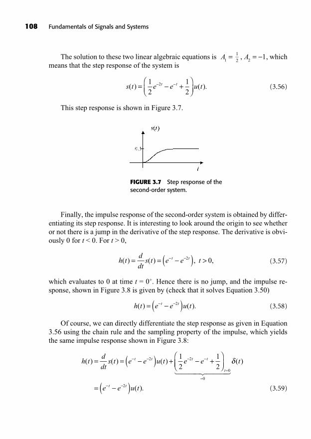
108 Fundamentals of Signals and Systems
The solution to these two linear algebraic equations is , whichmeans that the step response of the system is
(3.56)
This step response is shown in Figure 3.7.
s t e e u tt t( ) ( ).= − +⎛⎝⎜
⎞⎠⎟
− −1
2
1
22
A2
1= −,1
2A
1=
FIGURE 3.7 Step response of thesecond-order system.
Finally, the impulse response of the second-order system is obtained by differ-entiating its step response. It is interesting to look around the origin to see whetheror not there is a jump in the derivative of the step response. The derivative is obvi-ously 0 for t < 0. For t > 0,
(3.57)
which evaluates to 0 at time t = 0+. Hence there is no jump, and the impulse re-sponse, shown in Figure 3.8 is given by (check that it solves Equation 3.50)
(3.58)
Of course, we can directly differentiate the step response as given in Equation3.56 using the chain rule and the sampling property of the impulse, which yieldsthe same impulse response shown in Figure 3.8:
(3.59)
h td
dts t e e u t e et t t t( ) ( ) ( )= = −( ) + − +
⎛⎝
− − − −2 21
2
1
2⎜⎜⎞⎠⎟
= −( )=
=
− −
t
t t
t
e e u t
0
0
2
� ���� ����δ ( )
( ).
h t e e u tt t( ) ( ).= −( )− −2
h td
dts t e e tt t( ) ( ) , ,= = −( ) >− −2 0

((Lecture 11: Impulse Response of a Difference System; Characteristic Polynomialand Stability))
Differential and Difference LTI Systems 109
FIGURE 3.8 Impulse response obtainedby differentiating the step response.
IMPULSE RESPONSE OF A DIFFERENCE LTI SYSTEM
Consider the general form of a causal LTI difference system:
(3.60)
We briefly discuss one method to obtain the impulse response of this generalcausal LTI difference system initially at rest. It is similar to Method 1 for a contin-uous-time differential system, but it is simpler, as there is no integration involved.
Impulse Response Obtained by Linear Combination of Shifted Impulse Responsesof the Left-Hand Side of the Difference Equation
The step-by-step procedure to find the impulse response of a difference LTI systemis as follows.
1. Replace the whole right-hand side of the difference Equation 3.60 by δ[n].2. Find initial conditions on y[n] at times for a homoge-
neous response starting at time n = 1.3. Calculate the homogeneous response ha[n] to the homogeneous equation
with these initial conditions.4. Finally, calculate h[n] as a linear combination of the current and delayed
versions of ha[n] according to the right-hand side of the difference Equa-tion 3.60.
n N= − − +0 1 1, , ,…
a y n k b x n kk
k
N
kk
M
[ ] [ ].− = −= =∑ ∑
0 0

Step 1: Under the assumption that the system is initially at rest, that is,, let and replace the right-hand
side of Equation 3.60 with a single unit impulse:
(3.61)
Step 2: To solve this equation for ha[n], we first observe that, by causality,the impulse can only be part of ha[n], not its delayed versions ha[n – k], k ≠ 0.
This immediately gives us . Causality and the initial rest conditionyield the remaining initial conditions .Step 3: Thus, starting at time n = 1, we need to solve the homogeneous equa-tion for n > 0:
(3.62)
subject to the N initial conditions obtained in Step 2. Assume that the solutionhas the form of a complex exponential Czn for n > 0. Substituting this exponen-tial into Equation 3.62, we get a polynomial in z–1, multiplying an exponentialon the left-hand side. Dividing both sides by Czn and multiplying both sides byzN, we get an equivalent equation:
(3.63)
and this equation holds if and only if the characteristic polynomial
vanishes at the complex number z; that is,
(3.64)
By the fundamental theorem of algebra, this equation has at most N distinctroots. Assume that the N roots are distinct for simplicity and let them be denotedas . This means that there are N distinct exponential signals that sat-isfy the homogeneous Equation 3.62. Then the solution to Equation 3.62 can bewritten as a linear combination of these complex exponentials:
(3.65)h n C za k k
n
k
N
[ ] .==∑
1
C zk k
nzk k
N{ } =1
p z a z a z a z ak
N k
k
NN N
N( ) .= = + + + =−
=
−∑0
0 11 0�
a zk
N k−∑k
N
=∑
0
p z( ) :=
Cz a z a znk
k
k
N
kN k
k
N−
=
−
=∑ ∑= ⇔ =
0 0
0 0,
a h n kk a
k
N
[ ] ,− ==∑
0
0
h h h Na a a[ ] [ ] [ ]− = − = = − + =1 2 1 0�a
1
0
=ha[ ]0 =
a h n k nk a
k
N
[ ] [ ].− ==∑
0
δ
h n y na[ ] [ ]=y y y N[ ] [ ] [ ]− = − = = − =1 2 0�
110 Fundamentals of Signals and Systems
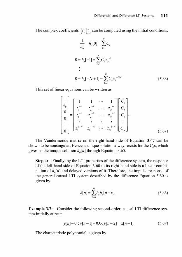
The complex coefficients can be computed using the initial conditions:
(3.66)
This set of linear equations can be written as
(3.67)
The Vandermonde matrix on the right-hand side of Equation 3.67 can beshown to be nonsingular. Hence, a unique solution always exists for the Cks, whichgives us the unique solution ha[n] through Equation 3.65.
Step 4: Finally, by the LTI properties of the difference system, the responseof the left-hand side of Equation 3.60 to its right-hand side is a linear combi-nation of ha[n] and delayed versions of it. Therefore, the impulse response ofthe general causal LTI system described by the difference Equation 3.60 isgiven by
(3.68)
Example 3.7: Consider the following second-order, causal LTI difference sys-tem initially at rest:
(3.69)
The characteristic polynomial is given by
y n y n y n x n[ ] . [ ] . [ ] [ ].− − + − = −0 5 1 0 06 2 1
h n b h n kk a
k
M
[ ] [ ].= −=∑
0
1
01
12
1
0
0
0
1 1 1a
z z zN
�
��
⎡
⎣
⎢⎢⎢⎢⎢⎢⎢⎢
⎤
⎦
⎥⎥⎥⎥⎥⎥⎥⎥
=
− − −−
− − −
− − −
⎡
⎣
⎢⎢⎢⎢⎢
1
12
22 2
11
21 1
z z z
z z z
N
N NN
N
�
� � � ��⎢⎢
⎤
⎦
⎥⎥⎥⎥⎥⎥
⎡
⎣
⎢⎢⎢⎢⎢⎢⎢
⎤
⎦
⎥⎥⎥⎥⎥⎥⎥
C
C
C
CN
1
2
3
�
.
0 1
0 1
1
1
1
1
= − =
= − + =
−
=
− +
=
∑h C z
h N C z
a k kk
N
a k kN
k
[ ]
[ ]
�NN
∑
10
0 1ah C
a kk
N
= ==∑[ ]
Ck k
N{ } =1
Differential and Difference LTI Systems 111
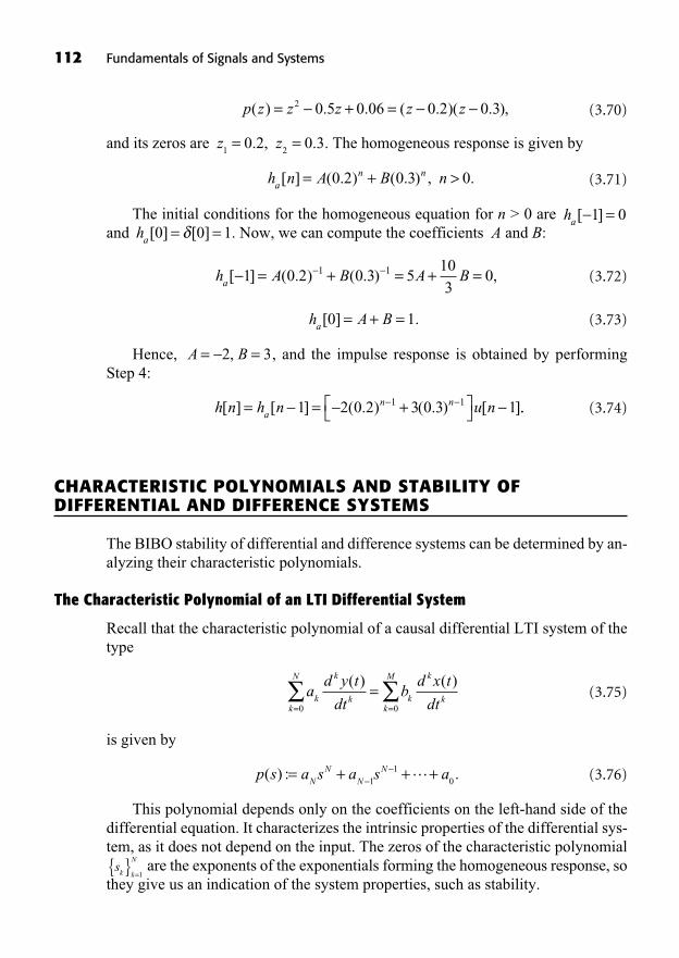
(3.70)
and its zeros are . The homogeneous response is given by
(3.71)
The initial conditions for the homogeneous equation for n > 0 are and . Now, we can compute the coefficients A and B:
(3.72)
(3.73)
Hence, , and the impulse response is obtained by performingStep 4:
(3.74)
CHARACTERISTIC POLYNOMIALS AND STABILITY OFDIFFERENTIAL AND DIFFERENCE SYSTEMS
The BIBO stability of differential and difference systems can be determined by an-alyzing their characteristic polynomials.
The Characteristic Polynomial of an LTI Differential System
Recall that the characteristic polynomial of a causal differential LTI system of thetype
(3.75)
is given by
(3.76)
This polynomial depends only on the coefficients on the left-hand side of thedifferential equation. It characterizes the intrinsic properties of the differential sys-tem, as it does not depend on the input. The zeros of the characteristic polynomial
are the exponents of the exponentials forming the homogeneous response, sothey give us an indication of the system properties, such as stability.
sk k
N{ } =1
p s a s a s aN
NN
N( ) : .= + + +−−
11
0�
ad y t
dtb
d x t
dtk
k
kk
N
k
k
kk
M( ) ( )
= =∑ ∑=
0 0
h n h n u nan n[ ] [ ] ( . ) ( . ) [ ]= − = − +⎡
⎣⎤⎦ −− −1 2 0 2 3 0 3 11 1 ..
A B= − =2 3,
h A Ba[ ] .0 1= + =
h A B A Ba[ ] ( . ) ( . ) ,− = + = + =− −1 0 2 0 3 5103
01 1
ha[ ] [ ]0 0 1= =δha[ ]− =1 0
h n A B nan n[ ] ( . ) ( . ) , .= + >0 2 0 3 0
z z1 2
0 2 0 3= =. , .
p z z z z z( ) . . ( . )( . ),= − + = − −2 0 5 0 06 0 2 0 3
112 Fundamentals of Signals and Systems
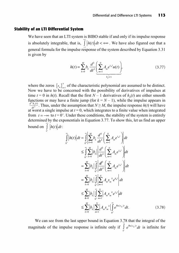
Stability of an LTI Differential System
We have seen that an LTI system is BIBO stable if and only if its impulse response
is absolutely integrable, that is, . We have also figured out that a
general formula for the impulse response of the system described by Equation 3.31is given by
(3.77)
where the zeros of the characteristic polynomial are assumed to be distinct.Now we have to be concerned with the possibility of derivatives of impulses attime t = 0 in h(t). Recall that the first N – 1 derivatives of ha(t) are either smoothfunctions or may have a finite jump (for k = N – 1), while the impulse appears in
. Thus, under the assumption that N ≥ M, the impulse response h(t) will haveat worst a single impulse at t = 0, which integrates to a finite value when integratedfrom to t = 0+. Under these conditions, the stability of the system is entirelydetermined by the exponentials in Equation 3.77. To show this, let us find an upper
bound on :
(3.78)
We can see from the last upper bound in Equation 3.78 that the integral of the
magnitude of the impulse response is infinite only if is infinite fore dts tmRe{ }
+∫
0+
∞
∫
h t dt bd
dtA e dt
k
k
k m
s t
m
N
k
Mm( )
0 100+
∞
==∫ ∑∑=
⎛⎝⎜
⎞⎠⎟++
+
∞
==
∞
∫
∑∑∫≤⎛⎝⎜
⎞⎠⎟
=
bd
dtA e dt
b
k
k
k m
s t
m
N
k
M
k
m
100
dd
dtA e dt
b A s e
k
k m
s t
m
N
k
M
k m mk
m
=
∞
=∑∫∑ ⎛
⎝⎜⎞⎠⎟
=
+ 100
ss t
m
N
k
M
k m mk s t
m
N
m
m
dt
b A s e dt
=
∞
=
=
∞
∑∫∑
∑∫
+
+
≤
100
10kk
M
k m mk s t
m
N
k
M
b A s e dtm
=
∞
==
∑
∫∑∑≤+
0
010
Re{ } .
h t dt( )∞
0+
+∞
∫
t = −∞
d h t
dt
NaN
( )
sm m
N{ } =1
h t bd
dtA e u t
k
k
k m
s t
m
N
h t
m
a
( ) ( )
( )
=⎛⎝⎜
⎞⎠⎟=
∑1� ��� ����k
M
=∑
0
,
h t dt( ) < +∞−∞
+∞
∫
Differential and Difference LTI Systems 113
some . This occurs only if . It can be shown that this nec-essary condition of stability is also sufficient modulo the next remark. That is, if atleast one of the zeros of the characteristic polynomial has a nonnegative real part,then the system is unstable.
With the earlier assumptions that the zeros of the characteristic polynomial aredistinct and that , a causal LTI differential system is BIBO stable if andonly if the real part of all of the zeros of its characteristic polynomial are negative(we say that they lie in the left half of the complex plane).
Remark: The purist might say that the causal differential system described by
(3.79)
is BIBO stable, even though the zero of its characteristic polynomial lies inthe right half of the complex plane. Indeed, if one computed the impulse responseof this system by using the procedure outlined above, one would get the identitysystem h(t) = δ(t), whose impulse response is absolutely integrable. Thus, strictlyspeaking, the system of Equation 3.79 is BIBO stable, but as engineers, we must beaware that even if the input signal is identically zero for all times, any nonzero ini-tial condition on the output signal, even infinitesimal, or any perturbation of the co-efficients will excite the unstable exponential et in the homogeneous response andwill drive the output to infinity. Therefore, this type of system must be consideredunstable. We will describe such systems in subsequent chapters as having a polecanceling a zero in the closed right half of the complex plane. A physical systemdescribed by such a differential equation will surely be unstable in practice.
Example 3.8: Let us assess the stability of the causal LTI differential system de-fined as
(3.80)
The characteristic polynomial is , which has its zero at s = 2. Thissystem is therefore BIBO unstable, which is easy to see with an impulse responseof the form Ae2tu(t ), a growing exponential.
The Characteristic Polynomial of an LTI Difference System
Recall that the characteristic polynomial of a causal difference LTI system of thetype
p s s( ) = − 2
dy t
dty t x t
( )( ) ( ).− =2
s1
1=
dy t
dty t
d
dtx t x t
( )( ) ( ) ( )− = −
N M≥
Re{ }sm
≥ 0m M∈{ }1, ,…
114 Fundamentals of Signals and Systems
(3.81)
is given by
(3.82)
This polynomial depends only on the coefficients on the left-hand side of the dif-ference equation. The zeros (assumed to be distinct) of the characteristicpolynomial are the arguments of the exponentials forming the homogeneous re-sponse, so they also give us an indication of system properties, such as stability.
Stability of an LTI Difference System
Recall that a discrete-time LTI system is stable if and only if its impulse response
is absolutely summable, that is, . For the causal difference system
above, this leads to the following upper bound:
(3.83)
and this last upper bound is finite if and only if for all . Hence,the causal LTI difference system is BIBO stable only if all the zeros of its charac-teristic polynomial have a magnitude less than 1. This necessary condition for
m N= 1, ,…zm<1,
h n b h n k
b h n k
nk a
k
M
n
k ak
[ ] [ ]
[ ]
=
+∞
==
+∞
=
∑ ∑∑= −
≤ −
0 00
000
0
M
n
k an kk
M
k m mn k
m
b h n k
b C z
∑∑
∑∑=
+∞
=
+∞
=
−
=
= −
=
[ ]
110
10
N
n kk
M
k m mn k
m
N
n kk
M
b C z
b
∑∑∑
∑∑∑=
+∞
=
−
==
+∞
=
≤
=kk m m
n k
n km
N
k
M
k m m
r
rm
N
C z
b C z
−
=
+∞
==
=
+∞
=
∑∑∑
∑=
10
01∑∑∑
=k
M
0
,
h n[ ] < +∞n=−∞
+∞
∑
zk k
N{ } =1
p z a z a z a z ak
N k
k
NN N
N( ) .= = + + + =−
=
−∑0
0 11 0�
a y n k b x n kk
k
N
kk
M
[ ] [ ]− = −= =∑ ∑
0 0
Differential and Difference LTI Systems 115

116 Fundamentals of Signals and Systems
stability turns out to be sufficient as well, and hence BIBO stability is equivalentto having all the zeros have a magnitude less than 1. Note that the previous remark also applies to discrete-time difference systems: a system of the type
must be considered unstable even though its im-pulse response is absolutely summable. Round-off errors in a digitalimplementation of such a difference system would destabilize it.
Example 3.9: Consider the causal first-order LTI difference system:
(3.84)
Its characteristic polynomial is , which has a single zero at. Hence, this system is stable, as . Its impulse response is
shown in Figure 3.9.z
10 9 1= <.z
10 9= .
p z z( ) .= − 0 9
y n y n x n[ ] . [ ] [ ].− − =0 9 1
h n n[ ] [ ]= δy n y n x n x n[ ] [ ] [ ] [ ]+ − = + −2 1 2 1
FIGURE 3.9 Impulse response of thefirst-order system.
TIME CONSTANT AND NATURAL FREQUENCY OF A FIRST-ORDER LTI DIFFERENTIAL SYSTEM
In general, the impulse response of an LTI differential system is a linear combina-tion of complex exponentials of the type and their derivatives. Considerthe stable, causal first-order LTI differential system:
(3.85)
Its impulse response is a single exponential, , where
and . The real number is called the natural frequency of the
first-order system, and its inverse is called the time constant of the1
0
a
a=
ω1
n
τ0
:=ω
ns:=
1
K
a1
A =
a
a0
1
s1= −h t Ae u ts t( ) ( )= 1
ady t
dta y t Kx t
1 0
( )( ) ( ).+ =
Ae u tst ( )
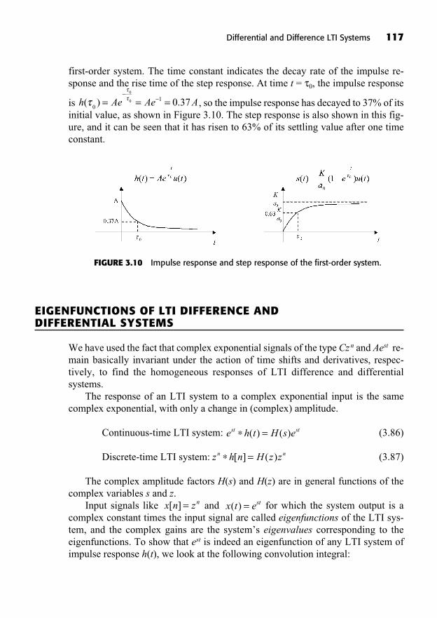
first-order system. The time constant indicates the decay rate of the impulse re-sponse and the rise time of the step response. At time t = τ0, the impulse response
is , so the impulse response has decayed to 37% of itsinitial value, as shown in Figure 3.10. The step response is also shown in this fig-ure, and it can be seen that it has risen to 63% of its settling value after one timeconstant.
h Ae Ae A( ) .τττ
01
0
0 0 37= = =−
−
Differential and Difference LTI Systems 117
FIGURE 3.10 Impulse response and step response of the first-order system.
EIGENFUNCTIONS OF LTI DIFFERENCE AND DIFFERENTIAL SYSTEMS
We have used the fact that complex exponential signals of the type Czn and Aest re-main basically invariant under the action of time shifts and derivatives, respec-tively, to find the homogeneous responses of LTI difference and differentialsystems.
The response of an LTI system to a complex exponential input is the samecomplex exponential, with only a change in (complex) amplitude.
Continuous-time LTI system: (3.86)
Discrete-time LTI system: (3.87)
The complex amplitude factors H(s) and H(z) are in general functions of thecomplex variables s and z.
Input signals like and for which the system output is acomplex constant times the input signal are called eigenfunctions of the LTI sys-tem, and the complex gains are the system’s eigenvalues corresponding to theeigenfunctions. To show that est is indeed an eigenfunction of any LTI system ofimpulse response h(t), we look at the following convolution integral:
x t est( ) =x n zn[ ] =
z h n H z zn n∗ =[ ] ( )
e h t H s est st∗ =( ) ( )
(3.88)
The system’s response has the form , where ,assuming the integral converges. For LTI discrete-time systems, the complex ex-ponential zn is an eigenfunction:
(3.89)
The system’s response has the form , where ,
assuming that the sum converges. The functions H(s) and H(z) are, respectively, theLaplace transform and the z-transform of the system’s impulse response. Each iscalled the transfer function of the system; more on this in Chapter 6 and Chapter 13.
SUMMARY
In this chapter, we introduced special classes of LTI systems: differential and dif-ference systems.
The classical solution composed of the sum of the forced response and the nat-ural response was reviewed for both differential and difference systems.Since an LTI system is completely characterized by its impulse response, wegave step-by-step techniques to compute the impulse responses of differentialand difference systems.The BIBO stability of differential and difference systems was analyzed withrespect to the characteristic polynomial.The time constant of a first-order differential system and its correspondingnatural frequency were introduced.Finally, it was pointed out that exponential signals are basically invariant (onlytheir complex amplitude varies) when processed by a differential or differencesystem.
h k z k[ ] −
k=−∞
+∞
∑H z( ) =y n H z zn[ ] ( )=
y n h k x n k h k z
z h
k
n k
k
n
[ ] [ ] [ ] [ ]
[
= − =
=
=−∞
+∞−
=−∞
+∞
∑ ∑
kk z k
k
] −
=−∞
+∞
∑
h e ds( ) −τ ττ
−∞
+∞
∫H s( ) :=y t H s est( ) ( )=
y t h x t d h e d
e
s t( ) ( ) ( ) ( ) ( )= − =
=
−∞
+∞−
−∞
+∞
∫ ∫τ τ τ τ ττ
sst sh e d( )τ ττ−
−∞
+∞
∫
118 Fundamentals of Signals and Systems
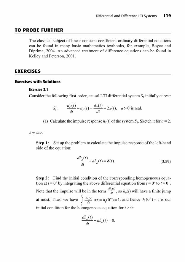
TO PROBE FURTHER
The classical subject of linear constant-coefficient ordinary differential equationscan be found in many basic mathematics textbooks, for example, Boyce andDiprima, 2004. An advanced treatment of difference equations can be found inKelley and Peterson, 2001.
EXERCISES
Exercises with Solutions
Exercise 3.1
Consider the following first-order, causal LTI differential system S1 initially at rest:
(a) Calculate the impulse response h1(t) of the system S1. Sketch it for a = 2.
Answer:
Step 1: Set up the problem to calculate the impulse response of the left-handside of the equation:
(3.59)
Step 2: Find the initial condition of the corresponding homogeneous equa-tion at t = 0+ by integrating the above differential equation from t = 0– to t = 0+.
Note that the impulse will be in the term , so ha(t) will have a finite jump
at most. Thus, we have , and hence is our
initial condition for the homogeneous equation for t > 0:
dh t
dtah ta
a
( )( ) .+ = 0
h1
0 1( )+ =d h ( )τ 1 0 1= =+dh
da ( )ττ
0
0
−
+
∫
dh t
dta ( )
dh t
dtah t ta
a
( )( ) ( ).+ = δ
Sdy t
dtay t
dx tdt
x t a1 2 0:( )
( )( )
( ),+ = − > is real.
Differential and Difference LTI Systems 119
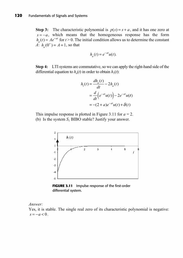
120 Fundamentals of Signals and Systems
Step 3: The characteristic polynomial is , and it has one zero at, which means that the homogeneous response has the form
for t > 0. The initial condition allows us to determine the constantA: , so that
Step 4: LTI systems are commutative, so we can apply the right-hand side of thedifferential equation to ha(t) in order to obtain h1(t):
This impulse response is plotted in Figure 3.11 for a = 2.(b) Is the system S1 BIBO stable? Justify your answer.
h tdh t
dth t
ddt
e u t e u
aa
at at
1 2
2
( )( )
( )
( ) (
= −
= ( ) −− − tt
a e u t tat
)
( ) ( ) ( )= − + +−2 δ
h t e u taat( ) ( ).= −
h Aa ( )0 1+ = =h t Aea
at( ) = −s a= −
p s s a( ) = +
FIGURE 3.11 Impulse response of the first-orderdifferential system.
Answer:Yes, it is stable. The single real zero of its characteristic polynomial is negative:
.s a= − < 0

Exercise 3.2
Consider the following second-order, causal LTI differential system S2 initially atrest:
Calculate the impulse response of the system S2.
Answer:Solution 1:
Step 1: Set up the problem to calculate the impulse response of the system:
Step 2: Find the initial conditions of the corresponding homogeneous equa-tion at t = 0+ by integrating the above differential equation from t = 0– to t = 0+.
Note that the impulse will be in the term , so dh2(t) will have a finite jumpat most. Thus we have
Hence, is one of our two initial conditions for the homogeneousequation for t > 0:
Since has a finite jump from t = 0– to t = 0+, the other initial condition is.
Step 3: The characteristic polynomial is and it has zeros at, which means that the homogeneous response has the form
for t > 0. The initial conditions allow us to determineconstants A and B:h t Ae Bet t
22 3( ) = +− −
s s1 22 3= − = −,p s s s( ) = + +2 5 6
h2 0 0( )+ =
dh t
dt2 ( )
d h t
dt
dh t
dth t
222
225 6 0
( ) ( )( ) .+ + =
1=dh
dt2 0( )+
d h
dd
dh
dt
22
2
0
02 0
1( ) ( )
.τ
ττ
−
+
∫ = =+
d h t
dt
222
( )
d h t
dt
dh t
dth t t
222
225 6
( ) ( )( ) ( )+ + = δ
Sd y t
dt
dy tdt
y t x t2
2
25 6:
( ) ( )( ) ( ).+ + =
Differential and Difference LTI Systems 121
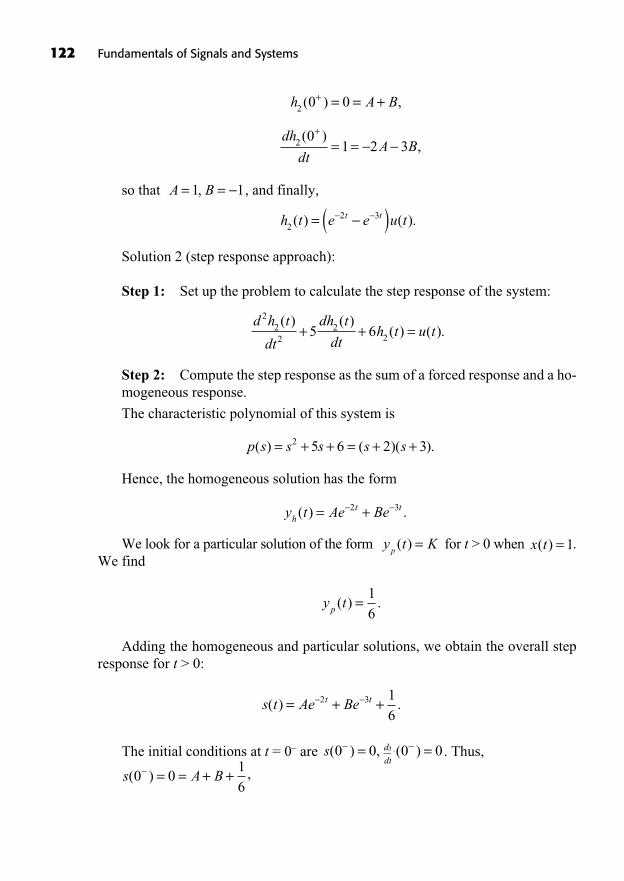
so that , and finally,
Solution 2 (step response approach):
Step 1: Set up the problem to calculate the step response of the system:
Step 2: Compute the step response as the sum of a forced response and a ho-mogeneous response.
The characteristic polynomial of this system is
Hence, the homogeneous solution has the form
We look for a particular solution of the form for t > 0 when .We find
Adding the homogeneous and particular solutions, we obtain the overall stepresponse for t > 0:
The initial conditions at t = 0– are . Thus,
,s A B( )0 016
− = = + +
( )0 0− =dsdt
s( ) ,0 0− =
s t Ae Bet t( ) .= + +− −2 3 16
y tp ( ) .= 16
x t( ) = 1y t Kp( ) =
y t Ae Beht t( ) .= +− −2 3
p s s s s s( ) ( )( ).= + + = + +2 5 6 2 3
d h t
dt
dh t
dth t u t
222
225 6
( ) ( )( ) ( ).+ + =
h t e e u tt t2
2 3( ) ( ).= −( )− −
A B= = −1 1,
dh
dtA B2 0
1 2 3( )
,+
= = − −
h A B2 0 0( ) ,+ = = +
122 Fundamentals of Signals and Systems
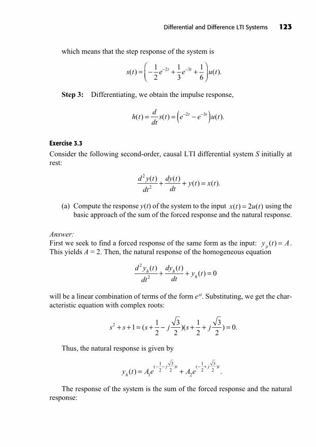
which means that the step response of the system is
Step 3: Differentiating, we obtain the impulse response,
Exercise 3.3
Consider the following second-order, causal LTI differential system S initially atrest:
(a) Compute the response y(t) of the system to the input using thebasic approach of the sum of the forced response and the natural response.
Answer:First we seek to find a forced response of the same form as the input: .This yields A = 2. Then, the natural response of the homogeneous equation
will be a linear combination of terms of the form est. Substituting, we get the char-acteristic equation with complex roots:
Thus, the natural response is given by
The response of the system is the sum of the forced response and the naturalresponse:
y t A e A eh
j t j t( ) .
( ) ( )= +
− − − +
1
12
32
2
12
32
s s s j s j2 112
32
12
32
0+ + = + − + + =( )( ) .
d y t
dt
dy t
dty th h
h
2
20
( ) ( )( )+ + =
y t Ap ( ) =
x t u t( ) ( )= 2
d y t
dt
dy tdt
y t x t2
2
( ) ( )( ) ( ).+ + =
h tddt
s t e e u tt t( ) ( ) ( ).= = −( )− −2 3
s t e e u tt t( ) ( ).= − + +⎛⎝⎜
⎞⎠⎟
− −12
13
16
2 3
Differential and Difference LTI Systems 123
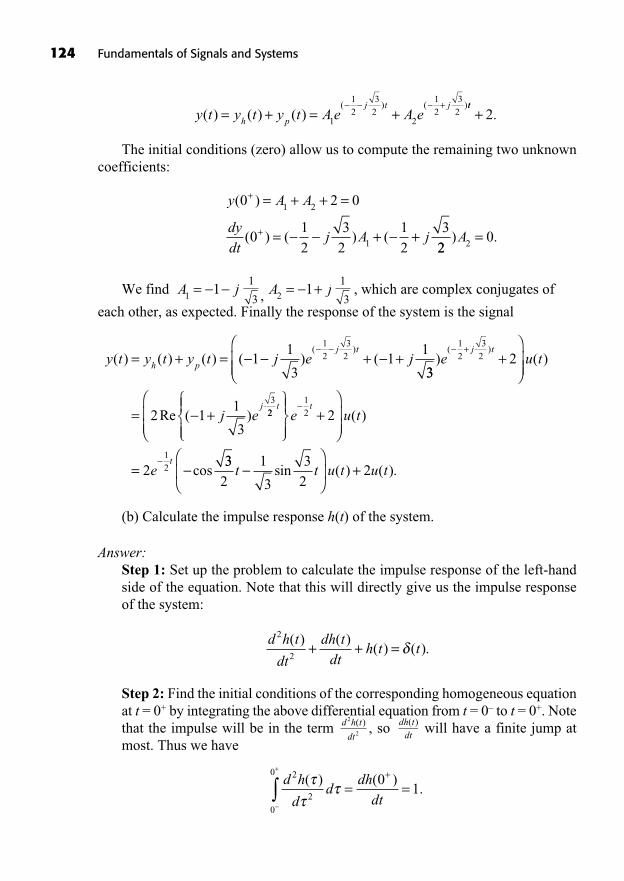
The initial conditions (zero) allow us to compute the remaining two unknowncoefficients:
We find , , which are complex conjugates of
each other, as expected. Finally the response of the system is the signal
(b) Calculate the impulse response h(t) of the system.
Answer:Step 1: Set up the problem to calculate the impulse response of the left-handside of the equation. Note that this will directly give us the impulse responseof the system:
Step 2: Find the initial conditions of the corresponding homogeneous equationat t = 0+ by integrating the above differential equation from t = 0– to t = 0+. Notethat the impulse will be in the term , so will have a finite jump atmost. Thus we have
d h
dd
dhdt
2
2
0
00
1( ) ( )
.τ
ττ
−
+
∫ = =+
dh tdt( )d h t
dt
2
2
( )
d h t
dt
dh tdt
h t t2
2
( ) ( )( ) ( ).+ + = δ
y t y t y t j e jh p
j t( ) ( ) ( ) ( ) (
( )= + = − − + − +
− −1
1
31
112
32
332
2 11
3
12
32
3
) ( )
Re ( )
( )e u t
j e
j t
j
− ++
⎛
⎝⎜⎜
⎞
⎠⎟⎟
= − + 2212
12
2
2
t t
t
e u t
e
⎧⎨⎪
⎩⎪
⎫⎬⎪
⎭⎪+
⎛
⎝⎜⎜
⎞
⎠⎟⎟
= −
−
−
( )
cos33
21
3
32
2t t u t u t−⎛
⎝⎜
⎞
⎠⎟ +sin ( ) ( ).
1
3A j2 1= − +1
3A j1 1= − −
y A A
dydt
j A j
( )
( ) ( ) (
0 2 0
012
32
12
3
1 2
1
+
+
= + + =
= − − + − +22
02) .A =
y t y t y t A e A eh p
j t j( ) ( ) ( )
( ) ( )= + = +
− − − +
1
12
32
2
12
32
tt+ 2.
124 Fundamentals of Signals and Systems
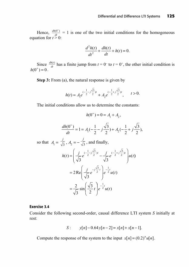
Hence, = 1 is one of the two initial conditions for the homogeneousequation for t > 0:
Since has a finite jump from t = 0– to t = 0+, the other initial condition is.
Step 3: From (a), the natural response is given by
The initial conditions allow us to determine the constants:
so that , and finally,
Exercise 3.4
Consider the following second-order, causal difference LTI system S initially atrest:
Compute the response of the system to the input .x n u nn[ ] ( . ) [ ]= 0 2
S y n y n x n x n: [ ] . [ ] [ ] [ ].− − = + −0 64 2 1
h tj
ej
e u tj t j t
( ) (( ) ( )
= −⎛
⎝⎜⎜
⎞
⎠⎟⎟
− − − +
3 3
12
32
12
32 ))
Re ( )
sin
=⎛
⎝⎜⎜
⎞
⎠⎟⎟
=⎛
⎝⎜
− −2
3
2
3
32
32
12j
e e u t
t
j t t
⎞⎞
⎠⎟
−e u t
t12 ( )
j
3A2 = −,j
3A1 =
dhdt
A j A j( )
( ) ( ),0
112
32
12
321 2
+
= = − − + − +
h A A( ) ,0 0 1 2+ = = +
t > 0.h t A e A ej t j t
( ) ,( ) ( )
= +− − − +
1
12
32
2
12
32
h( )0 0+ =
dh tdt( )
d h t
dt
dh tdt
h t2
20
( ) ( )( ) .+ + =
dhdt( )0+
Differential and Difference LTI Systems 125

Answer:The characteristic polynomial is , with zeros
. The homogeneous response is given by
The forced response for n ≥ 1 has the form :
Notice here that we assume that n ≥ 1 so that all the terms on the right-handside of the difference equation are present in the computation of the coefficient C.The assumption of initial rest implies , but we need to use initialconditions at times when the forced response exists (for n ≥ 1), that is, y[1], y[2],which can be obtained by a simple recursion:
Now, we can compute the coefficients A and B:
This yields . Finally, the overall response is
y n u nn n n[ ] . ( . ) . ( . ) . ( . ) [= − − + −⎡⎣
⎤⎦0 1 0 8 1 5 0 8 0 4 0 2 ]].
A B= − =0 1 1 5. , .
y A B
A
[ ] ( . ) ( . ) . ( . ) .
.
1 0 8 0 8 0 4 0 2 1 2
0 8 0
1 1 1= − + − =⇒ − + .. .
[ ] ( . ) ( . ) . ( . ) .
8 1 28
2 0 8 0 8 0 4 0 2 02 2 2
B
y A B
== − + − = 888
0 64 0 64 0 896⇒ + =. . .A B
y n y n u n u n
n
n n[ ] . [ ] ( . ) [ ] ( . ) [ ]= − + + −
=
−0 64 2 0 2 0 2 11
00 0 0 64 0 0 2 0 1
1 1 0 64 0
0: [ ] . ( ) ( . )
: [ ] . ( )
y
n y
= + + =
= = + (( . ) ( . ) .
: [ ] . ( ) ( . ) (
0 2 0 2 1 2
2 2 0 64 1 0 2
1 0
2
+ =
= = + +n y 00 2 0 881. ) . .=
y y[ ] [ ]− = − =2 1 0
C C
C
n n n n( . ) . ( . ) ( . ) ( . )
( .
0 2 0 64 0 2 0 2 0 2
1 0
2 1− = +
−
− −
664 0 2 1 0 2
615
0 4
2 1( . ) ) ( . )
. .
− −= +
=−
= −C
y n Cpn[ ] ( . )= 0 2
h n A B nan n[ ] ( . ) ( . ) , .= − + ≥0 8 0 8 0
z z1 20 8 0 8= − =. , .z z z2 0 64 0 8 0 8− = − +. ( . )( . )
126 Fundamentals of Signals and Systems
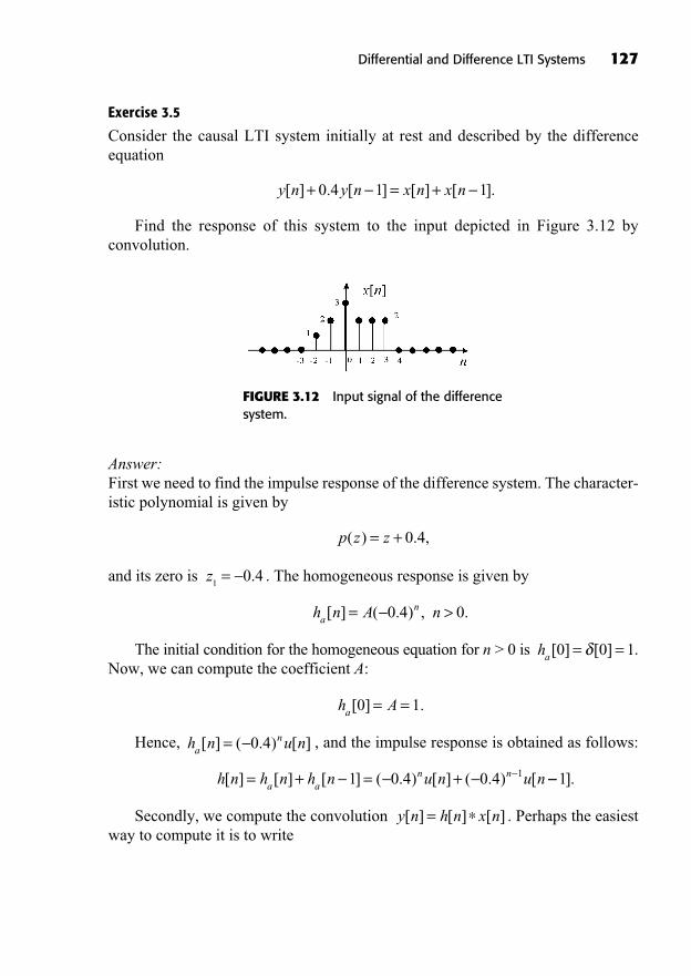
Exercise 3.5
Consider the causal LTI system initially at rest and described by the differenceequation
Find the response of this system to the input depicted in Figure 3.12 byconvolution.
y n y n x n x n[ ] . [ ] [ ] [ ].+ − = + −0 4 1 1
Differential and Difference LTI Systems 127
FIGURE 3.12 Input signal of the differencesystem.
Answer:First we need to find the impulse response of the difference system. The character-istic polynomial is given by
and its zero is . The homogeneous response is given by
The initial condition for the homogeneous equation for n > 0 is .Now, we can compute the coefficient A:
Hence, , and the impulse response is obtained as follows:
Secondly, we compute the convolution . Perhaps the easiestway to compute it is to write
y n h n x n[ ] [ ] [ ]= ∗
h n h n h n u n u na an n[ ] [ ] [ ] ( . ) [ ] ( . ) [= + − = − + − −1 0 4 0 4 1 −−1].
h n u nan[ ] ( . ) [ ]= −0 4
h Aa[ ] .0 1= =
ha[ ] [ ]0 0 1= =δ
h n A nan[ ] ( . ) , .= − >0 4 0
z1
0 4= − .
p z z( ) . ,= + 0 4
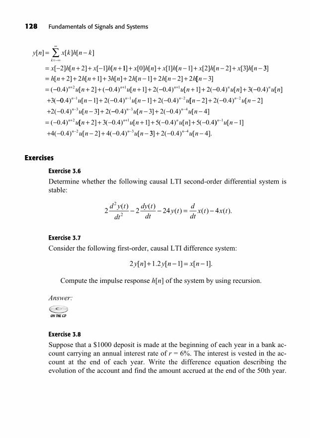
128 Fundamentals of Signals and Systems
Exercises
Exercise 3.6
Determine whether the following causal LTI second-order differential system isstable:
Exercise 3.7
Consider the following first-order, causal LTI difference system:
Compute the impulse response h[n] of the system by using recursion.
Answer:
Exercise 3.8
Suppose that a $1000 deposit is made at the beginning of each year in a bank ac-count carrying an annual interest rate of r = 6%. The interest is vested in the ac-count at the end of each year. Write the difference equation describing theevolution of the account and find the amount accrued at the end of the 50th year.
2 1 2 1 1y n y n x n[ ] . [ ] [ ].+ − = −
2 2 24 42
2
d y t
dt
dy tdt
y tddt
x t x t( ) ( )
( ) ( ) ( ).− − = −
y n x k h n k
x h n x h nk
[ ] [ ] [ ]
[ ] [ ] [ ] [
= −
= − + + − +=−∞
∞
∑2 2 1 11 0 1 1 2 2 3] [ ] [ ] [ ] [ ] [ ] [ ] [ ] [+ + − + − + −x h n x h n x h n x h n 33
2 2 1 3 2 1 2 2 2
]
[ ] [ ] [ ] [ ] [ ]= + + + + + − + − +h n h n h n h n h n h[[ ]
( . ) [ ] ( . ) [ ] (
n
u n u nn n
−= − + + − + + −+ +
3
0 4 2 0 4 1 2 02 1 .. ) [ ] ( . ) [ ] ( . ) [ ]
(
4 1 2 0 4 3 0 4
3
1n n nu n u n u n+ + + − + −+ −00 4 1 2 0 4 1 2 0 41 1 2. ) [ ] ( . ) [ ] ( . )n n nu n u n u− − −− + − − + − [[ ] ( . ) [ ]
( . ) [ ] (
n u n
u n
n
n
− + − −+ − − +
−
−
2 2 0 4 2
2 0 4 3 2
2
3 −− − + − −= −
− −
+
0 4 3 2 0 4 4
0 4
3 4
2
. ) [ ] ( . ) [ ]
( . )
n n
n
u n u n
u[[ ] ( . ) [ ] ( . ) [ ] ( .n u n u nn n+ + − + + − + −+2 3 0 4 1 5 0 4 5 0 41 )) [ ]
( . ) [ ] ( . ) [
n
n n
u n
u n u n
−
− −
−+ − − + − −
1
2 3
1
4 0 4 2 4 0 4 33 2 0 4 44] ( . ) [ ].+ − −−n u n
Differential and Difference LTI Systems 129
Exercise 3.9
Find the impulse response h(t) of the following second-order, causal LTI differen-tial system:
Answer:
Exercise 3.10
Compute and sketch the impulse response h(t) of the following causal LTI, first-order differential system initially at rest:
Exercise 3.11
Compute the impulse response h[n] of the following causal LTI, second-order dif-ference system initially at rest:
Simplify your expression of h[n] to obtain a real function of time.
Answer:
Exercise 3.12
Calculate the impulse response h(t) of the following second-order, causal LTI dif-ferential system initially at rest:
d y t
dt
dy tdt
y tdx t
dtx t
2
22 2 3
( ) ( )( )
( )( ).+ + = − +
y n y n y n x n x n[ ] [ ] [ ] [ ] [ ].+ − + − = − + −3 1 2 1 2
2 4 3 2dy t
dty t
ddt
x t x t( )
( ) ( ) ( ).+ = +
d y t
dt
dy tdt
y tdx t
dtx t
2
22
( ) ( )( )
( )( ).+ + = +
130 Fundamentals of Signals and Systems
Exercise 3.13
Consider the following second-order, causal difference LTI system S initially at rest:
(a) What is the characteristic polynomial of S? What are its zeros? Is the sys-tem stable?
(b) Compute the impulse response of S for all n.
(c) Compute the response of S for all n for the input signal x[n] = 2u[n] usingthe conventional solution (sum of particular solution and homogeneous solution).
Answer:
S y n y n y n x n: [ ] . [ ] . [ ] [ ].− − + − = −0 9 1 0 2 2 1

131
Fourier Series Representationof Periodic Continuous-TimeSignals
In This Chapter
Linear Combinations of Harmonically Related Complex ExponentialsDetermination of the Fourier Series Representation of a Continuous-Time Periodic SignalGraph of the Fourier Series Coefficients: The Line SpectrumProperties of Continuous-Time Fourier SeriesFourier Series of a Periodic Rectangular WaveOptimality and Convergence of the Fourier SeriesExistence of a Fourier Series RepresentationGibbs PhenomenonFourier Series of a Periodic Train of ImpulsesParseval TheoremPower SpectrumTotal Harmonic DistortionSteady-State Response of an LTI System to a Periodic SignalSummaryTo Probe FurtherExercises
((Lecture 12: Definition and Properties of the Fourier Series))
Asignal is defined as a function of time representing the evolution of a vari-able. Certain types of signals have the special property of remaining basi-cally invariant under the action of linear time-invariant systems. Such
signals include sinusoids and exponential functions of time. These signals can belinearly combined to form virtually any other signal, which is the basis of theFourier series representation of periodic signals and the Fourier transform repre-sentation of aperiodic signals.
4
132 Fundamentals of Signals and Systems
The Fourier representation opens up a whole new interpretation of signals interms of their frequency contents, called their frequency spectrum. Furthermore, inthe frequency domain, a linear time-invariant system acts as a filter on the fre-quency spectrum of the input signal, attenuating it at some frequencies while am-plifying it at other frequencies. This property is called the frequency response ofthe system. These frequency domain concepts are fundamental in electrical engi-neering, as they underpin the fields of communication systems, analog and digitalfilter design, feedback control, power engineering, etc.
Well-trained electrical and computer engineers think of signals in terms oftheir frequency spectrum probably just as much as they think of them as functionsof time.
LINEAR COMBINATIONS OF HARMONICALLY RELATEDCOMPLEX EXPONENTIALS
Recall that periodic signals satisfy for some positivevalue of T. The smallest such T is called the fundamental period of the signal, andits fundamental frequency is defined as . One thing to remember isthat the periodic signal x(t ) is entirely determined by its values over one period T.Also recall that we looked at harmonically related complex exponentials with fre-quencies that are integer multiples of 0:
(4.1)
We saw that these harmonically related signals have a very important property:they form an orthogonal set. That is,
(4.2)
Each of these signals has a fundamental frequency that is a multiple of 0, andtherefore each is periodic with period T (although for , the fundamental pe-riod of is T ). Let us look at the imaginary part of for and
shown in Figure 4.1.T = 1sk = 0 1 2, ,
kt( )k
t( )k >1
k mjk t jm tt t dt e e dt e( ) ( ) = =
0
2
0
2
0
0 0
0
jj m k t
j m k
dt
j m ke
( )
( )
( )=
0
0
0
2
0
211 ==
=2
00
,
,
.m k
m k
kjk tt e k( ) : , , , , .= = ± ±0 0 1 2…
rad s2
T0=
x t x t T t( ) ( ),= + < < +

Fourier Series Representation of Periodic Continuous-Time Signals 133
A linear combination of the complex exponentials is also periodic withfundamental period T:
(4.3)
The two terms with in this series are collectively called the fundamen-tal components, or the first harmonic components, of the signal. The two termswith are referred to as the second harmonic components (with fundamen-tal frequency ), and more generally the components for are called theNth harmonic components.
Example 4.1: Consider the periodic signal with fundamental frequencymade up of the sum of five harmonic components:
(4.4)
Collecting the harmonic components together, we obtain
(4.5)
x t e e e ej t j t j t
( ) . ( ) . (= + +0 2026 0 02252 232
jj t j t j te e
32
52
520 0081
0 4052
) . ( )
. cos(
+
=22
0 04503
20 0162
5
2t t t) . cos( ) . cos( )
x t a e
a a a
k
jk t
k
( ) ,
, . , ,
=
= = ==
± ±
2
5
5
0 1 20 0 2026 0
aa a a± ± ±= = =3 4 5
0 0225 0 0 0081. , , . .
02= rad/s
k N= ±20
k = ±2
k = ±1
x t a e a ek
jk t
kk
jkT
t
k
( ) .( )
= ==
+
=
+0
2
kt( )
FIGURE 4.1 Imaginary parts of complex harmonics.
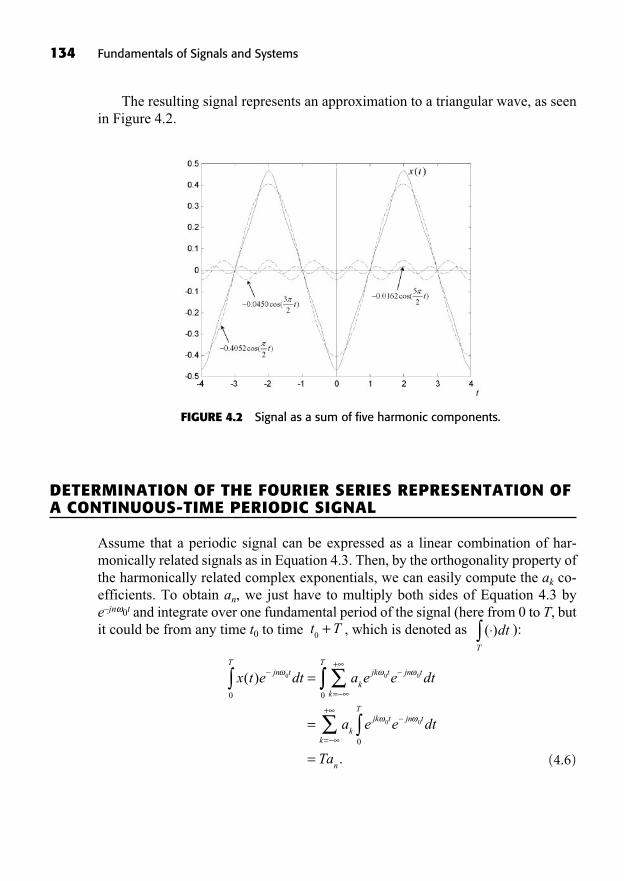
134 Fundamentals of Signals and Systems
The resulting signal represents an approximation to a triangular wave, as seenin Figure 4.2.
FIGURE 4.2 Signal as a sum of five harmonic components.
DETERMINATION OF THE FOURIER SERIES REPRESENTATION OFA CONTINUOUS-TIME PERIODIC SIGNAL
Assume that a periodic signal can be expressed as a linear combination of har-monically related signals as in Equation 4.3. Then, by the orthogonality property ofthe harmonically related complex exponentials, we can easily compute the ak co-efficients. To obtain an, we just have to multiply both sides of Equation 4.3 bye–jn 0t and integrate over one fundamental period of the signal (here from 0 to T, butit could be from any time t0 to time , which is denoted as ):
(4.6)
x t e dt a e e dtjn tT
k
jk t jn t
k
T
( )=
+
=0 0 0
0 0
=
==
+
a e e dt
Ta
k
jk t jn tT
k
n
0 0
0
.
( )dtT
t T0+
Thus,
To recap, if a periodic signal x(t ) has a Fourier series representation, then wehave the equation pair
(4.7)
(4.8)
which gives us two representations of the signal. Equation 4.7 is a time-domainrepresentation of the signal as a sum of periodic complex exponential signals. Thisis the synthesis equation. Equation 4.8, called the analysis equation, gives us a fre-quency-domain representation of the signal as the Fourier series coefficients, alsoreferred to as the spectral coefficients of x(t ). That is, each one of these complexcoefficients tells us how much the corresponding harmonic component of a givenfrequency contributes to the signal.
Remarks:The coefficient is the DC component of the signal (average
value of the signal over one period). It should always be computed separatelyfrom ak to avoid indeterminacies of the type 0/0 in the expression for ak eval-uated at .For a real signal x(t), we have . Let . Then wehave a real form of the Fourier series:
(4.9)
For a real signal x(t ), if we represent the Fourier series coefficients as, we obtain another real form of the Fourier series:a B jC B Ck k k k k= + , , R
x t a e a a e a ek
jk t
kk
jk t
k
jk t( ) = = + +=
+0 0 0
0kk
k
jk t
k
k
a a e
a A k
=
+
=
+
= +
= +
1
01
0
2
2
0Re{ }
cos(00
1
tk
k
+=
+
).
a A e Ak kj
k kk= , , Ra a
k k=
k = 0
x t dt( )T T
1a0=
aT
x t e dtT
x t e dtk
jk t
T
jkT
t
T
= =1 1
0
2
( ) ( ) ,( )
x t a e a ek
jk t
kk
jkT
t
k
( ) ,( )
= ==
+
=
+0
2
aT
x t e dtn
jn tT
=1
0
0
( ) .
Fourier Series Representation of Periodic Continuous-Time Signals 135
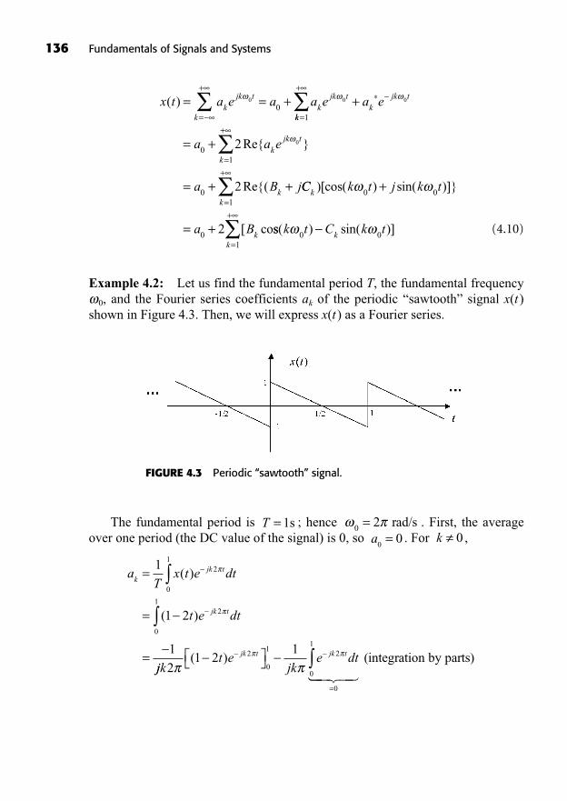
136 Fundamentals of Signals and Systems
FIGURE 4.3 Periodic “sawtooth” signal.
The fundamental period is ; hence . First, the averageover one period (the DC value of the signal) is 0, so . For ,
aT
x t e dt
t e dt
kjk t
jk t
=
=
=
1
1 2
1
2
0
1
2
0
1
( )
( )
jjkt e
jke dtjk t jk t
21 2
12
0
12
0
1
0
( )
=�� �� ��
(integration by parts)
k 0a0
0=0 2= rad/sT = 1s
(4.10)
Example 4.2: Let us find the fundamental period T, the fundamental frequency0, and the Fourier series coefficients ak of the periodic “sawtooth” signal x(t )
shown in Figure 4.3. Then, we will express x(t ) as a Fourier series.
x t a e a a e a ekjk t
kk
jk tk
jk t( ) = = + +=
+0 0 0
0kk
kjk t
k
k
a a e
a B j
=
+
=
+
= +
= + +
1
01
0
2
2
0Re{ }
Re{( CC k t j k t
a B
kk
k
)[cos( ) sin( )]}
[ co
0 01
0 2
+
= +
=
+
ss( ) sin( )]k t C k tkk
0 01=
+
(4.11)
Note that the coefficients are purely imaginary and form an oddsequence, which is consistent with our real, odd signal. The Fourier series repre-sentation of x(t ) is
(4.12)
GRAPH OF THE FOURIER SERIES COEFFICIENTS: THE LINE SPECTRUM
The set of complex Fourier series coefficients of a signal can be plottedwith separate graphs for their magnitude and phase. The combination of both plotsis called the line spectrum of the signal.
Example 4.3: Consider the Fourier series coefficients of the sawtooth signal obtained in the previous example. Their magnitudes are given by ,
, and , and their phases are given by and
. The corresponding line spectrum is shown in Figure 4.4.
The following MATLAB M-file located in D:\Chapter4\linespectrum.m dis-plays the line spectrum of the sawtooth signal.
=a0
0
=>
<a
k
kk
20
20
,
,
a0
0=k 0
k=
1a
k=
{ }ak k=
+
x t a ej
ke
kjk t
k
jk t
kk
( ) .= ==
+
=
+2 2
0
j
ka
k=
= +
=
1
2
1
2
1
jk jk
jjk
j
k= .
Fourier Series Representation of Periodic Continuous-Time Signals 137

138 Fundamentals of Signals and Systems
%% Line spectrum of Fourier series coefficients
% signal amplitude and period
A=1;
T=1;
% number of harmonics
N=10;
% first compute the ak’s
a0=0;
spectrum=zeros(1,2*N+1);
for k=-N:N
% spectral coefficients of sawtooth signal
if k>0
eval([‘a’ num2str(k) ‘=-j*A/(k*pi)’])
eval([‘spectrum(k+N+1)=a’ num2str(k)]);
elseif k<0
eval([‘a_’ num2str(abs(k)) ‘=-j*A/(k*pi)’])
eval([‘spectrum(k+N+1)=a_’ num2str(abs(k))]);
end
FIGURE 4.4 Line spectrum of the sawtooth signal.
eval([‘spectrum(N+1)=a0’]);
end
% line spectrum
K=[-N:N];
subplot(211)
stem(K,abs(spectrum),’.-’)
subplot(212)
stem(K,phase(spectrum),’.-’)
Remark: A common mistake is to forget that the magnitude line spectrum mustalways be nonnegative. This mistake might arise, for example, when one writes
, which is obviously wrong since k can be negative.
PROPERTIES OF CONTINUOUS-TIME FOURIER SERIES
Note that if the periodic signal x(t ) admits a Fourier series representation, then itsset of spectral coefficients determines x(t ) completely. The duality be-tween the signal and its spectral representation is denoted as . The fol-lowing properties of the Fourier series are easy to show using Equations 4.7 and4.8. (Do it as an exercise.) Note that these properties are also listed in Table D.3 ofAppendix D.
Linearity
The operation of calculating the Fourier series coefficients of a periodic signal
is linear. For , , if we form the linear combination, , then
(4.13)
Time Shifting
Time shifting leads to a multiplication by a complex exponential. For ,
(4.14)x t t e aFS jk t
k( ) .
00 0
x t aFS
k( )
z t a bFS
k k( ) .+
, Cz t x t y t( ) ( ) ( )= +y t b
FS
k( )x t a
FS
k( )
x t aFS
k( )
{ }ak k=
+
k=
1a
k=
Fourier Series Representation of Periodic Continuous-Time Signals 139
Remark: The magnitudes of the Fourier series coefficients are not changed, onlytheir phases.
Time Reversal
Time reversal leads to a “sequence reversal” of the corresponding sequence ofFourier series coefficients:
(4.15)
Interesting consequences are that
For x(t ) even, the sequence of coefficients is also even ( ).For x(t ) odd, the sequence of coefficients is also odd ( ).
Time Scaling
Time scaling applied on a periodic signal changes the fundamental frequency of the signal (but it remains periodic “with the same shape”). For example, hasfundamental frequency and fundamental period –1T. The Fourier series co-efficients do not change:
(4.16)
but the Fourier series itself has changed, as the harmonic components are now atthe frequencies .
Application: For a given periodic signal (a specific waveform) such as a squarewave, one can compute the Fourier series coefficients for a single normalized fun-damental frequency. Then, the Fourier series of a square wave of any frequency hasthe same coefficients.
Multiplication of Two Signals
Suppose that x(t ) and y(t ) are both periodic with period T. For ,
, we have
(4.17)x t y t a bFS
l k ll
( ) ( ) ,=
+
y t bFS
k( )
x t aFS
k( )
± ± ±0 0 0
2 3, , ,…
x t aFS
k( ) ,
0
x t( )
a ak k=
a ak k=
x t aFS
k( ) .
140 Fundamentals of Signals and Systems
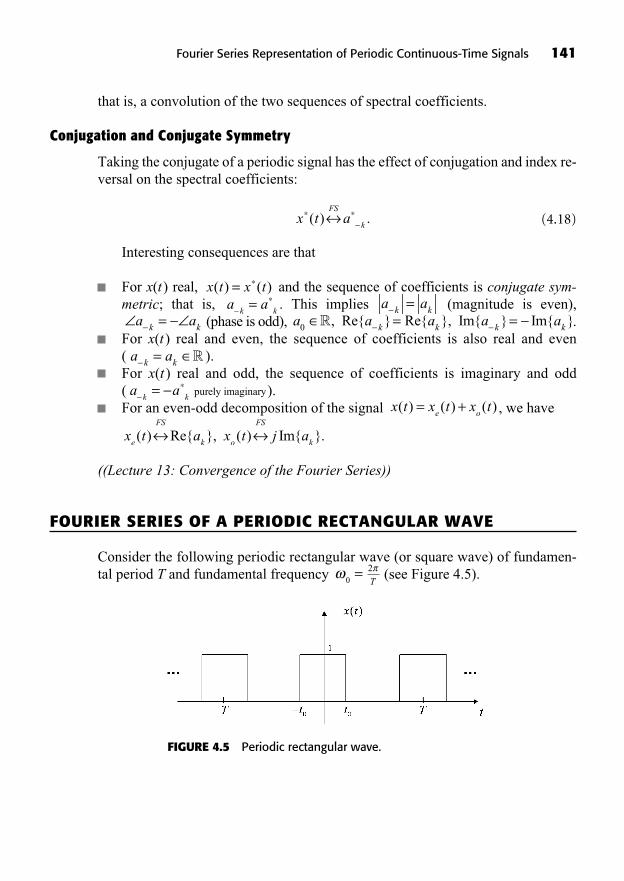
Fourier Series Representation of Periodic Continuous-Time Signals 141
that is, a convolution of the two sequences of spectral coefficients.
Conjugation and Conjugate Symmetry
Taking the conjugate of a periodic signal has the effect of conjugation and index re-versal on the spectral coefficients:
(4.18)
Interesting consequences are that
For x(t) real, and the sequence of coefficients is conjugate sym-metric; that is, . This implies (magnitude is even),
(phase is odd), .For x(t ) real and even, the sequence of coefficients is also real and even( ).For x(t ) real and odd, the sequence of coefficients is imaginary and odd( ).For an even-odd decomposition of the signal , we have
.
((Lecture 13: Convergence of the Fourier Series))
FOURIER SERIES OF A PERIODIC RECTANGULAR WAVE
Consider the following periodic rectangular wave (or square wave) of fundamen-tal period T and fundamental frequency (see Figure 4.5).2
T0=
x t a x t j ae
FS
k o
FS
k( ) Re{ }, ( ) Im{ }
x t x t x te o
( ) ( ) ( )= +a a
k k= purely imaginary
a ak k= R
a a a a ak k k k0 = =R, Re{ } Re{ }, Im{ } Im{ }=a ak k
a ak k=a ak k=
x t x t( ) ( )=
x t aFS
k( ) .
FIGURE 4.5 Periodic rectangular wave.
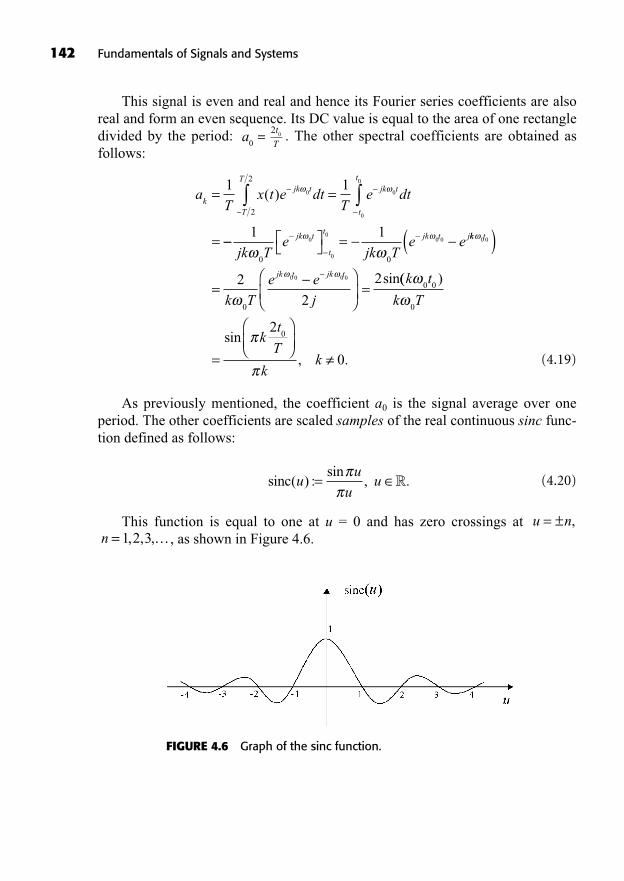
142 Fundamentals of Signals and Systems
This signal is even and real and hence its Fourier series coefficients are alsoreal and form an even sequence. Its DC value is equal to the area of one rectangledivided by the period: . The other spectral coefficients are obtained as follows:
(4.19)
As previously mentioned, the coefficient a0 is the signal average over oneperiod. The other coefficients are scaled samples of the real continuous sinc func-tion defined as follows:
(4.20)
This function is equal to one at u = 0 and has zero crossings at , as shown in Figure 4.6. n = , , ,1 2 3…
u n= ± ,
sin ( ) :sin
, .c uu
uu= �
aT
x t e dtT
e dtk
jk t
T
Tjk t
t
t
= =
=
1 10 0
0
0
2
2
( )
=1 1
0 0
0
0
00 0
jk Te
jk Te ejk t
t
tjk t jkk t
jk t jk t
k T
e e
j
0 0
0 0 0 02
2
2
0
( )= =
sin(( )
sin
, .
k t
k T
kt
T
kk
0 0
0
02
0=
t
T0
2a
0=
FIGURE 4.6 Graph of the sinc function.
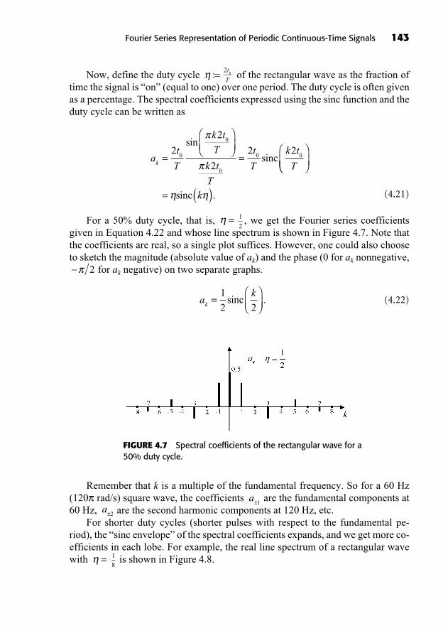
Now, define the duty cycle of the rectangular wave as the fraction oftime the signal is “on” (equal to one) over one period. The duty cycle is often givenas a percentage. The spectral coefficients expressed using the sinc function and theduty cycle can be written as
(4.21)
For a 50% duty cycle, that is, , we get the Fourier series coefficientsgiven in Equation 4.22 and whose line spectrum is shown in Figure 4.7. Note thatthe coefficients are real, so a single plot suffices. However, one could also chooseto sketch the magnitude (absolute value of ak) and the phase (0 for ak nonnegative,
for ak negative) on two separate graphs.
(4.22)ak
k=
1
2 2sinc .
2
=1
2=
at
T
k t
T
k t
T
t
T
k t
Tk= =
2
2
2
2 20
0
0
0 0
sin
sinc
= ( )sinc k .
20
t
T:=
Fourier Series Representation of Periodic Continuous-Time Signals 143
FIGURE 4.7 Spectral coefficients of the rectangular wave for a50% duty cycle.
Remember that k is a multiple of the fundamental frequency. So for a 60 Hz(120 rad/s) square wave, the coefficients are the fundamental components at60 Hz, are the second harmonic components at 120 Hz, etc.
For shorter duty cycles (shorter pulses with respect to the fundamental pe-riod), the “sinc envelope” of the spectral coefficients expands, and we get more co-efficients in each lobe. For example, the real line spectrum of a rectangular wavewith is shown in Figure 4.8.=
1
8=
a±2
a±1
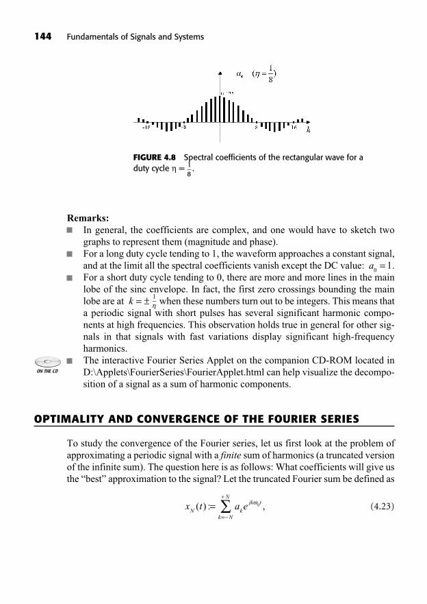
144 Fundamentals of Signals and Systems
Remarks:In general, the coefficients are complex, and one would have to sketch twographs to represent them (magnitude and phase).For a long duty cycle tending to 1, the waveform approaches a constant signal,and at the limit all the spectral coefficients vanish except the DC value: .For a short duty cycle tending to 0, there are more and more lines in the mainlobe of the sinc envelope. In fact, the first zero crossings bounding the mainlobe are at when these numbers turn out to be integers. This means thata periodic signal with short pulses has several significant harmonic compo-nents at high frequencies. This observation holds true in general for other sig-nals in that signals with fast variations display significant high-frequencyharmonics.The interactive Fourier Series Applet on the companion CD-ROM located inD:\Applets\FourierSeries\FourierApplet.html can help visualize the decompo-sition of a signal as a sum of harmonic components.
OPTIMALITY AND CONVERGENCE OF THE FOURIER SERIES
To study the convergence of the Fourier series, let us first look at the problem ofapproximating a periodic signal with a finite sum of harmonics (a truncated versionof the infinite sum). The question here is as follows: What coefficients will give usthe “best” approximation to the signal? Let the truncated Fourier sum be defined as
(4.23)x t a eN k
jk t
k N
N
( ) : ,==
+0
±1
k = ±
a0
1=
FIGURE 4.8 Spectral coefficients of the rectangular wave for aduty cycle = .= 1
8
Fourier Series Representation of Periodic Continuous-Time Signals 145
and define the approximation error as
(4.24)
Now, consider the energy in one period of the error signal as the quantity tominimize to get the best approximation.
(4.25)
We proceed by first expanding this equation:
(4.26)
Then, we write the coefficients in rectangular coordinates andseek to minimize the energy by taking its partial derivatives with re-spect to k and k and setting them equal to zero. Let us do it for the real part k:
(4.27)
Differentiating with respect to k, we obtain
(4.28)
This equation is satisfied with . Similarly, minimizing the
energy of the approximation error with respect to k yields .
Therefore, the complex coefficients minimize the approxi-mation error.
x t e dtjk t0( )T
T1
0
ak=
jk tT
Tx t e dt( )
10
0k= Im
jk tT
Tx t e dt( )
10
0k= Re
==
+ET x t e dtN
kk
k N
Njk t
T
2 2 0
0
Re ( ) ==
+
k N
N
0.
E x t dt T j x tN
T
k kk N
N
k k= + +
=
+
( ) ( ) ( ) (2
0
2 2 )) ( ) ( )e dt j x t e dtjk tT
k N
N
k k
jk t
=
+
+0 0
0 00
2
0
2 2 2
T
k N
N
T
k kk N
N
x t dt T
=
+
=
+
= + +( ) ( )kk
jk tT
k N
N
kx t e dtRe ( ) Im
=
+0
0
2 xx t e dtjk tT
k N
N
( ) .=
+0
0
EN k k
( , )a j
k k k= +
E x t a e x t a eN kjk t
k N
N
kjk=
=
+
( ) ( )0 00
0
0
t
k N
NT
T
kjk
dt
x t x t dt a e
=
+
= +( ) ( ) 00 0
0
t
k N
N
njn t
n N
NT
a e dt=
+
=
+
=
+
x t a e dt x t a ekjk t
k N
NT
kjk t( ) ( )0 0
0 kk N
NT
T
k nj k n t
dt
x t dt a a e dt
=
+
= +
0
2
0 0
0( ) ( )TT
n N
N
k N
N
kjk t
T
k N
N
a x t e dt==
+
=
+
( ) 0
0
= +
=
+
a x t e dt
x t dt T a a
kjk t
T
k N
N
T
k
( )
( )
0
0
2
0kk
k N
N
kjk t
T
k N
N
ka x t e dt a x=
+
=
+
( ) (0
0
tt e dtjk tT
k N
N
) .0
0=
+
E e t dtN N
T
= ( ) .2
e t x t x t x t a eN N k
jk t
k N
N
( ) : ( ) ( ) ( ) .= ==
+0
If the signal x(t) has a Fourier series representation, then the limit of the energy
in the approximation error as N tends to infinity is zero. In thissense, the Fourier series converges to the signal x(t ).
EXISTENCE OF A FOURIER SERIES REPRESENTATION
What classes of periodic signals have Fourier series representation? One that doesis the class of periodic signals with finite energy over one period (finite total aver-age power), that is, signals for which
(4.29)
These signals have Fourier series that converge in the sense that the power inthe difference between the signal and its Fourier series representation is zero. Notethat this does not imply that the signal x(t ) and its corresponding Fourier series areequal at every value of time t. The class of periodic signals with finite energy overone period is broad and quite useful for us.
Another broad class of signals that have Fourier series representation are sig-nals that satisfy the three Dirichlet conditions. These signals equal their Fourierseries representation, except at isolated values of t where x(t ) has finite disconti-nuities. At these times, the Fourier series converges to the average of the signalvalues on either side of the discontinuity.
Dirichlet Conditions
Condition 1: Over any period, x(t) must be absolutely integrable; that is,
.
Condition 2: In any finite interval of time, x(t ) must be of bounded varia-tions. This means that x(t ) must have a finite number of maxima and minimaduring any single period.
Example 4.4: The signal does not meet this require-ment, as it has an infinite number of oscillations as time approaches zero.
Condition 3: In any finite interval of time, x(t ) has a finite number of dis-continuities. Furthermore, each of these discontinuities is finite.
t, <0 1tn
2x t( ) sin=
x t dtT
( ) <
x t dtT
( ) .2
<
e t dtN
( )2
T
EN=
146 Fundamentals of Signals and Systems
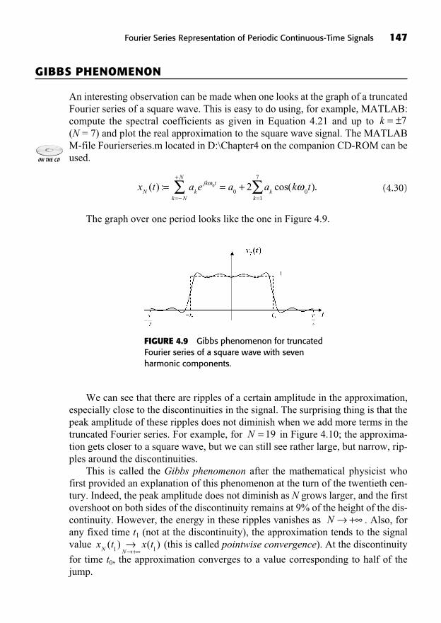
Fourier Series Representation of Periodic Continuous-Time Signals 147
GIBBS PHENOMENON
An interesting observation can be made when one looks at the graph of a truncatedFourier series of a square wave. This is easy to do using, for example, MATLAB:compute the spectral coefficients as given in Equation 4.21 and up to (N = 7) and plot the real approximation to the square wave signal. The MATLABM-file Fourierseries.m located in D:\Chapter4 on the companion CD-ROM can beused.
(4.30)
The graph over one period looks like the one in Figure 4.9.
x t a e a a k tN k
jk t
k N
N
kk
( ) : cos( )= = +=
+
=
0
0 01
7
2 ..
k = ±7
FIGURE 4.9 Gibbs phenomenon for truncatedFourier series of a square wave with sevenharmonic components.
We can see that there are ripples of a certain amplitude in the approximation,especially close to the discontinuities in the signal. The surprising thing is that thepeak amplitude of these ripples does not diminish when we add more terms in thetruncated Fourier series. For example, for in Figure 4.10; the approxima-tion gets closer to a square wave, but we can still see rather large, but narrow, rip-ples around the discontinuities.
This is called the Gibbs phenomenon after the mathematical physicist whofirst provided an explanation of this phenomenon at the turn of the twentieth cen-tury. Indeed, the peak amplitude does not diminish as N grows larger, and the firstovershoot on both sides of the discontinuity remains at 9% of the height of the dis-continuity. However, the energy in these ripples vanishes as . Also, forany fixed time t1 (not at the discontinuity), the approximation tends to the signalvalue (this is called pointwise convergence). At the discontinuity
for time t0, the approximation converges to a value corresponding to half of thejump.
x t x tN N
( ) ( )1 1+
N +
N = 19
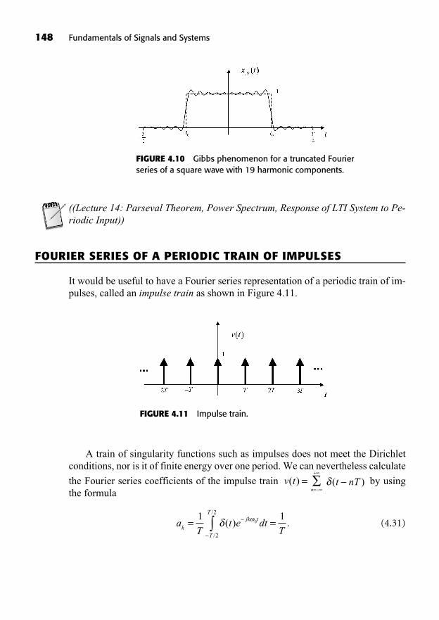
148 Fundamentals of Signals and Systems
((Lecture 14: Parseval Theorem, Power Spectrum, Response of LTI System to Pe-riodic Input))
FOURIER SERIES OF A PERIODIC TRAIN OF IMPULSES
It would be useful to have a Fourier series representation of a periodic train of im-pulses, called an impulse train as shown in Figure 4.11.
FIGURE 4.10 Gibbs phenomenon for a truncated Fourierseries of a square wave with 19 harmonic components.
FIGURE 4.11 Impulse train.
A train of singularity functions such as impulses does not meet the Dirichletconditions, nor is it of finite energy over one period. We can nevertheless calculate
the Fourier series coefficients of the impulse train by usingthe formula
(4.31)aT
t e dtTk
jk t
T
T
= =1 1
0
2
2
( ) ./
/
t nT( )n=
+
v t( ) =
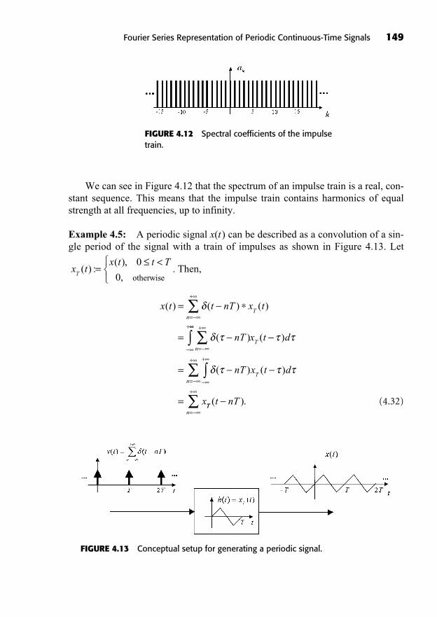
We can see in Figure 4.12 that the spectrum of an impulse train is a real, con-stant sequence. This means that the impulse train contains harmonics of equalstrength at all frequencies, up to infinity.
Example 4.5: A periodic signal x(t ) can be described as a convolution of a sin-gle period of the signal with a train of impulses as shown in Figure 4.13. Let
. Then,
(4.32)
x t t nT x t
nT
nT
n
( ) ( ) ( )
( )
=
=
=
+
=
++
+
=
+
=
=
x t d
nT x t d
x
T
Tn
( )
( ) ( )
TTn
t nT( ).=
+
x tx t t T
T( ) :
( ),
,=
<0
0 otherwise
Fourier Series Representation of Periodic Continuous-Time Signals 149
FIGURE 4.12 Spectral coefficients of the impulsetrain.
FIGURE 4.13 Conceptual setup for generating a periodic signal.
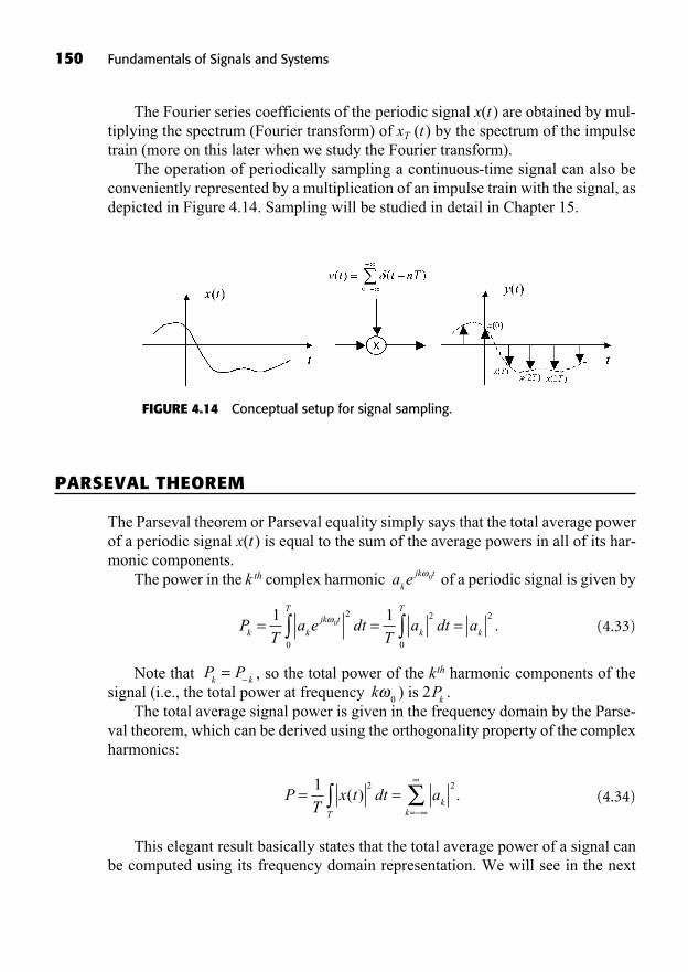
The Fourier series coefficients of the periodic signal x(t ) are obtained by mul-tiplying the spectrum (Fourier transform) of xT (t ) by the spectrum of the impulsetrain (more on this later when we study the Fourier transform).
The operation of periodically sampling a continuous-time signal can also beconveniently represented by a multiplication of an impulse train with the signal, asdepicted in Figure 4.14. Sampling will be studied in detail in Chapter 15.
150 Fundamentals of Signals and Systems
FIGURE 4.14 Conceptual setup for signal sampling.
PARSEVAL THEOREM
The Parseval theorem or Parseval equality simply says that the total average powerof a periodic signal x(t ) is equal to the sum of the average powers in all of its har-monic components.
The power in the k th complex harmonic of a periodic signal is given by
(4.33)
Note that , so the total power of the kth harmonic components of thesignal (i.e., the total power at frequency ) is .
The total average signal power is given in the frequency domain by the Parse-val theorem, which can be derived using the orthogonality property of the complexharmonics:
(4.34)
This elegant result basically states that the total average power of a signal canbe computed using its frequency domain representation. We will see in the next
PT
x t dt aT
kk
= ==
1 2 2( ) .
2Pk
k0
P Pk k=
PT
a e dtT
a dt ak k
jk tT
k
T
k= = =
1 10
2
0
2
0
2.
a ek
jk t0
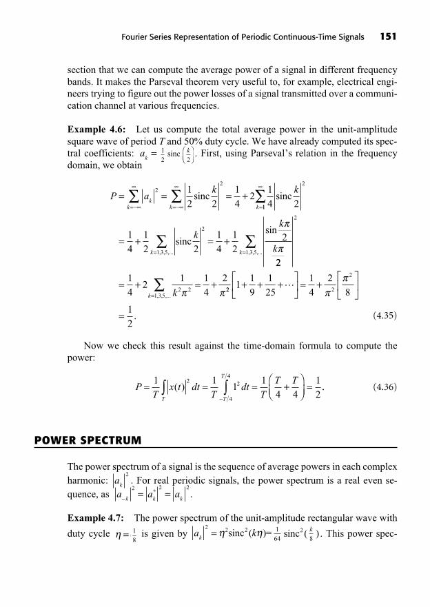
section that we can compute the average power of a signal in different frequencybands. It makes the Parseval theorem very useful to, for example, electrical engi-neers trying to figure out the power losses of a signal transmitted over a communi-cation channel at various frequencies.
Example 4.6: Let us compute the total average power in the unit-amplitudesquare wave of period T and 50% duty cycle. We have already computed its spec-tral coefficients: . First, using Parseval’s relation in the frequencydomain, we obtain
(4.35)
Now we check this result against the time-domain formula to compute thepower:
(4.36)
POWER SPECTRUM
The power spectrum of a signal is the sequence of average powers in each complexharmonic: . For real periodic signals, the power spectrum is a real even se-quence, as .
Example 4.7: The power spectrum of the unit-amplitude rectangular wave with
duty cycle is given by . This power spec-)k
82sinc (1
64a k
k
2 2 2= sinc ( )==1
8=
a a ak k k
= =2 2 2
ak
2
PT
x t dtT
dtT
T T
T T
T
= = = + =1 1
11
4 4
1
2
2 2
4
4
( ) ..
P ak k
kk k k
= = = += = =
22 2
1
2 2
1
42
1
4 2sinc sinc
11
2
1 3 5
1
4
1
2 2
1
4
1
22
=
= + = +sincsink
k
kk , , ,...
22
1
42
1
4
2
2
1 3 5
2 21 3 5
k
k k
=
=
= + = +
, , ,...
, , ,...
122 2
2
11
9
1
25
1
4
2
8
1
2
+ + + = +
=
.
k
2sinc1
2a
k=
Fourier Series Representation of Periodic Continuous-Time Signals 151
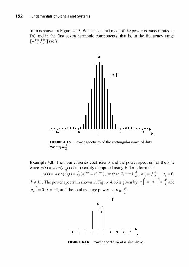
152 Fundamentals of Signals and Systems
trum is shown in Figure 4.15. We can see that most of the power is concentrated atDC and in the first seven harmonic components, that is, in the frequency range
.] rad/s,14 14
T T[
FIGURE 4.15 Power spectrum of the rectangular wave of dutycycle = .1
8
Example 4.8: The Fourier series coefficients and the power spectrum of the sinewave can be easily computed using Euler’s formula:
, so that
. The power spectrum shown in Figure 4.16 is given by and
, and the total average power is .A2
2P =a kk
20 1= ±,
A2
4a a
1
2
1
2= =k 1±
ak
0=, ,A
2a j1=,
A
2a j
1=e ej t j t( )0 0
A
j2x t A t( ) sin( )= =0
x t A t( ) sin( )=0
FIGURE 4.16 Power spectrum of a sine wave.
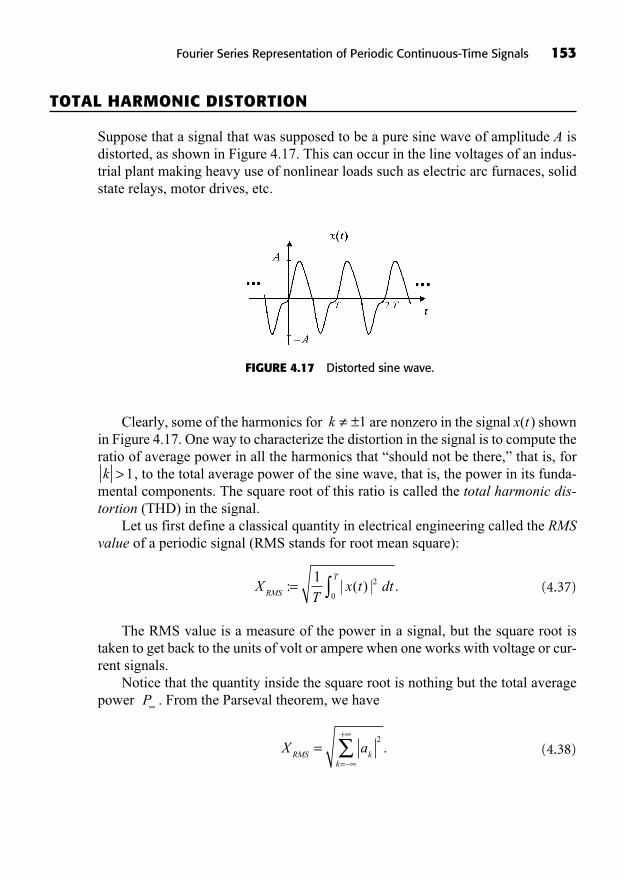
TOTAL HARMONIC DISTORTION
Suppose that a signal that was supposed to be a pure sine wave of amplitude A isdistorted, as shown in Figure 4.17. This can occur in the line voltages of an indus-trial plant making heavy use of nonlinear loads such as electric arc furnaces, solidstate relays, motor drives, etc.
Fourier Series Representation of Periodic Continuous-Time Signals 153
FIGURE 4.17 Distorted sine wave.
Clearly, some of the harmonics for are nonzero in the signal x(t) shownin Figure 4.17. One way to characterize the distortion in the signal is to compute theratio of average power in all the harmonics that “should not be there,” that is, for
, to the total average power of the sine wave, that is, the power in its funda-mental components. The square root of this ratio is called the total harmonic dis-tortion (THD) in the signal.
Let us first define a classical quantity in electrical engineering called the RMSvalue of a periodic signal (RMS stands for root mean square):
(4.37)
The RMS value is a measure of the power in a signal, but the square root istaken to get back to the units of volt or ampere when one works with voltage or cur-rent signals.
Notice that the quantity inside the square root is nothing but the total averagepower . From the Parseval theorem, we have
(4.38)X aRMS k
k
==
+2.
P
XT
x t dtRMS
T: | ( ) | .=
1 2
0
k >1
k ±1
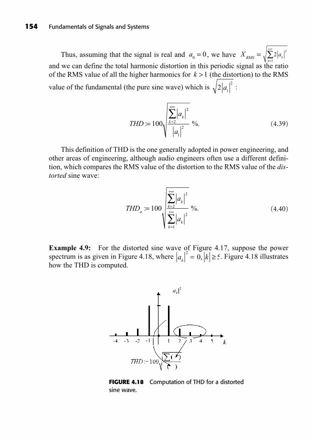
Thus, assuming that the signal is real and , we have
and we can define the total harmonic distortion in this periodic signal as the ratioof the RMS value of all the higher harmonics for (the distortion) to the RMS
value of the fundamental (the pure sine wave) which is :
(4.39)
This definition of THD is the one generally adopted in power engineering, andother areas of engineering, although audio engineers often use a different defini-tion, which compares the RMS value of the distortion to the RMS value of the dis-torted sine wave:
(4.40)
Example 4.9: For the distorted sine wave of Figure 4.17, suppose the powerspectrum is as given in Figure 4.18, where . Figure 4.18 illustrateshow the THD is computed.
a kk
20 5= ,
THDa
aa
kk
kk
: %.= =
+
=
+100
2
2
2
1
THDa
a
kk: %.= =
+
100
2
2
1
2
21
2a
k >1
ak
k=
+
22
1
XRMS
=a0
0=
154 Fundamentals of Signals and Systems
FIGURE 4.18 Computation of THD for a distortedsine wave.
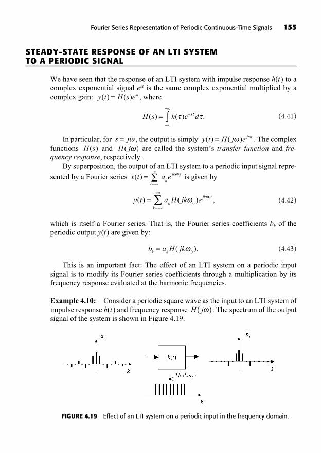
STEADY-STATE RESPONSE OF AN LTI SYSTEM TO A PERIODIC SIGNAL
We have seen that the response of an LTI system with impulse response h(t ) to acomplex exponential signal est is the same complex exponential multiplied by acomplex gain: , where
(4.41)
In particular, for , the output is simply . The complexfunctions and are called the system’s transfer function and fre-quency response, respectively.
By superposition, the output of an LTI system to a periodic input signal repre-
sented by a Fourier series is given by
(4.42)
which is itself a Fourier series. That is, the Fourier series coefficients bk of theperiodic output y(t ) are given by:
(4.43)
This is an important fact: The effect of an LTI system on a periodic inputsignal is to modify its Fourier series coefficients through a multiplication by itsfrequency response evaluated at the harmonic frequencies.
Example 4.10: Consider a periodic square wave as the input to an LTI system ofimpulse response h(t ) and frequency response . The spectrum of the outputsignal of the system is shown in Figure 4.19.
H j( )
b a H jkk k= ( ).
0
y t a H jk ek
jk t
k
( ) ( ) ,==
+
00
a ek
jk t0
k=
+
x t( ) =
H j( )H s( )y t H j e j t( ) ( )=s j=
H s h e ds( ) ( ) .=+
y t H s est( ) ( )=
Fourier Series Representation of Periodic Continuous-Time Signals 155
FIGURE 4.19 Effect of an LTI system on a periodic input in the frequency domain.
Remarks:It is assumed that the system is in steady-state; that is, it has been submitted tothe same input from time . Thus, there is no transient response from ini-tial conditions in the output signal.If the system is unstable, then the output would tend to infinity, so we assumethat the system is stable.
Filtering
Filtering is based on the concepts described earlier. Filtering a periodic signal withan LTI system involves the design of a filter with a desirable frequency spectrum
that retains certain frequencies and cuts off others.
Example 4.11: A first-order lowpass filter with impulse response (a simple RC circuit with ) cuts off the high-frequency harmonics in aperiodic input signal, while low-frequency harmonics are mostly left intact. Thefrequency response of this filter is computed as follows:
(4.44)
We can see that as the frequency increases, the magnitude of the frequency
response of the filter decreases. If the periodic input signal is a
unit-amplitude rectangular wave of duty cycle , then the output signal will haveits Fourier series coefficients bk given by:
(4.45)
(4.46)
The reduced power at high frequencies produces an output signal that is“smoother” than the input signal. Remember that discontinuities can only resultfrom a significant contribution of high-frequency harmonic components in theFourier series, so when these harmonics are filtered out, the result is a smoothersignal, as shown in Figure 4.20.
b a H a0 0 0
0= = =( ) .
b a H jkk
jkk
k k= =
+( )
( )
( ), ,
00
10
sinc
+
1
1 2H j( ) =
H j e e dj
j( ) = =+
+
0
1
1
RC = 1h t e u tt( ) ( )=
H jk( )0
t =
156 Fundamentals of Signals and Systems

Fourier Series Representation of Periodic Continuous-Time Signals 157
SUMMARY
This chapter introduced the frequency-domain interpretation of periodic continu-ous-time signals.
We have shown that most periodic continuous-time signals can be decom-posed as an infinite sum of complex harmonics using the Fourier series. Theseinclude finite-power signals and signals satisfying the Dirichlet conditions.Complex harmonics are periodic complex exponential signals of fundamentalfrequency equal to an integer times the fundamental frequency of the signal.These harmonics were shown to be orthogonal.The line spectrum and power spectrum plots of a periodic signal are based onits Fourier series coefficients and indicate the relative importance of the dif-ferent harmonic components making up the signal. The total harmonic distor-tion in a signal approximating a pure sine wave can be computed from thepower spectrum of the signal.The Gibbs phenomenon was shown to produce oscillations in the truncatedFourier series approximation of a signal around first-order discontinuities.Finally, filtering was introduced as the action of an LTI system on the Fourierseries coefficients of the input signal to either amplify or attenuate the har-monic components at different frequencies.
TO PROBE FURTHER
Further information on Fourier series can be found in Brown and Churchill, 2001.
FIGURE 4.20 Effect of a first-order, low-pass filter on arectangular wave.
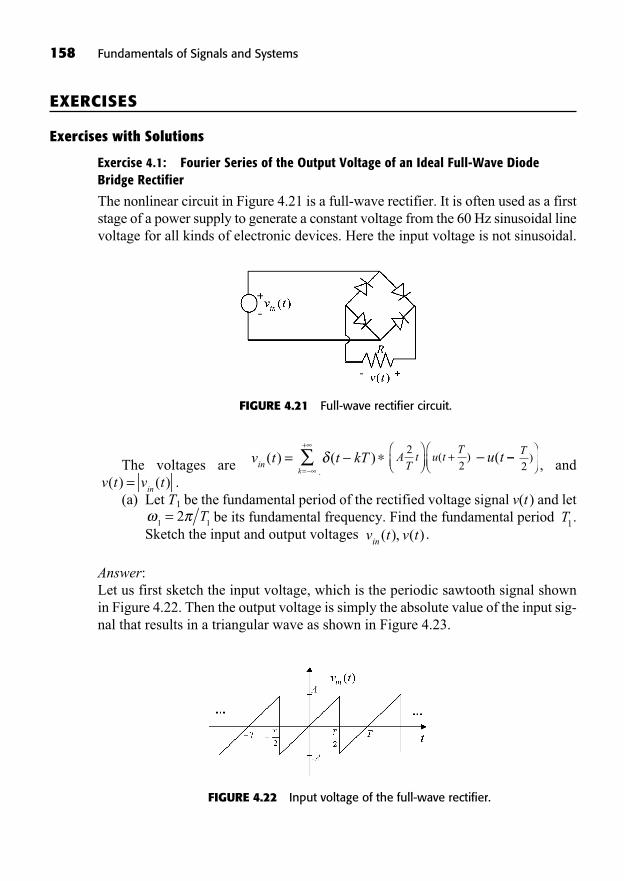
158 Fundamentals of Signals and Systems
EXERCISES
Exercises with Solutions
Exercise 4.1: Fourier Series of the Output Voltage of an Ideal Full-Wave DiodeBridge Rectifier
The nonlinear circuit in Figure 4.21 is a full-wave rectifier. It is often used as a firststage of a power supply to generate a constant voltage from the 60 Hz sinusoidal linevoltage for all kinds of electronic devices. Here the input voltage is not sinusoidal.
FIGURE 4.21 Full-wave rectifier circuit.
The voltages are , and.
(a) Let T1 be the fundamental period of the rectified voltage signal v(t ) and letbe its fundamental frequency. Find the fundamental period .
Sketch the input and output voltages .
Answer:Let us first sketch the input voltage, which is the periodic sawtooth signal shownin Figure 4.22. Then the output voltage is simply the absolute value of the input sig-nal that results in a triangular wave as shown in Figure 4.23.
v t v tin ( ), ( )T11 1
2= T
v t v tin
( ) ( )=
T2
)u t(AT
t u tT
( )+22
t kT( )k=
+
v tin ( ) =
FIGURE 4.22 Input voltage of the full-wave rectifier.
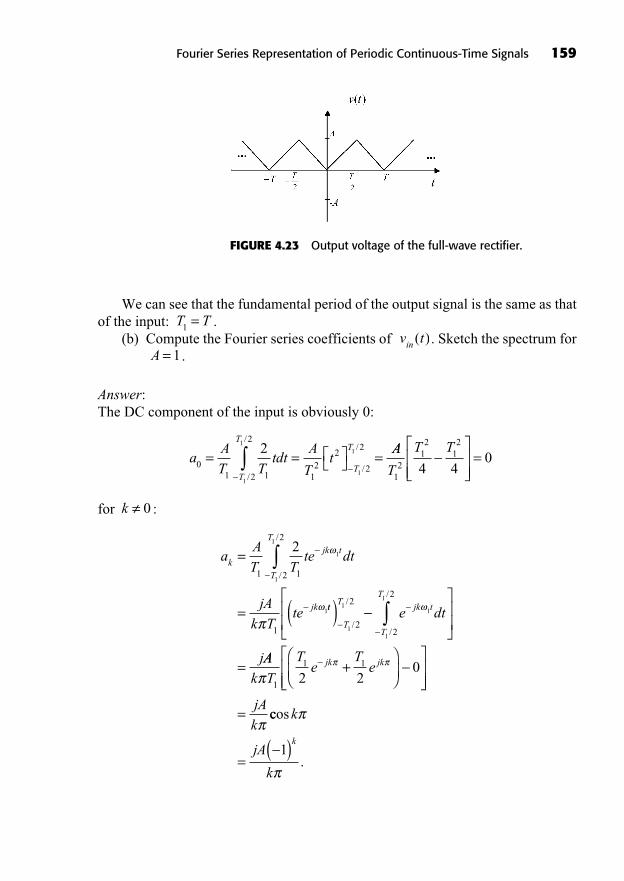
We can see that the fundamental period of the output signal is the same as thatof the input: .
(b) Compute the Fourier series coefficients of . Sketch the spectrum for.
Answer:The DC component of the input is obviously 0:
for :
aAT T
te dt
jAk T
te
kjk t
T
T
jk
=
=
1 12
2
1
21
1
1
1
/
/
tt
T
Tjk t
T
T
e dt
j
( )
=
1
11
1
1
2
2
2
2
/
/
/
/
AAk T
Te
Te
jAk
jk jk
1
1 1
2 20+
= ccos
.
k
jA
k
k
=( )1
k 0
aAT T
tdtA
Tt
T
T
T
T
01 12
2
12
2
2
22
1
1
1
1= = =/
/
/
/ AA
T
T T
12
12
12
4 40=
A = 1v tin ( )
T T1 =
Fourier Series Representation of Periodic Continuous-Time Signals 159
FIGURE 4.23 Output voltage of the full-wave rectifier.
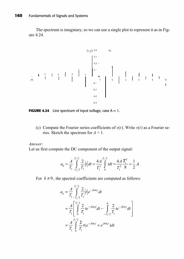
160 Fundamentals of Signals and Systems
The spectrum is imaginary, so we can use a single plot to represent it as in Fig-ure 4.24.
FIGURE 4.24 Line spectrum of input voltage, case A = 1.
(c) Compute the Fourier series coefficients of v(t ). Write v(t ) as a Fourier se-ries. Sketch the spectrum for A = 1.
Answer:Let us first compute the DC component of the output signal:
For , the spectral coefficients are computed as follows:
aAT T
t e dt
AT T
te
kjk t
T
T
jk
=
=
1 12
2
1 1
2
2
1
1
1
1
/
/
ttT
jk t
T
dtT
te dt
AT
0
2
12
0
1
1
1
1
2/
/
= 22
10
2
1 1
1
Tt e e dtjk t jk t
T
( )/
+
k 0
aAT T
t dtA
Ttdt
A
TT
T T
01 12
2
12
0
2
12
2 4 4
1
1 1
= = =/
/ /TT
A12
812
= .
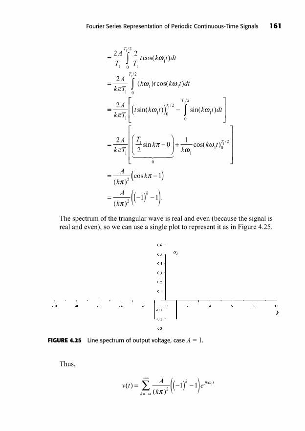
The spectrum of the triangular wave is real and even (because the signal isreal and even), so we can use a single plot to represent it as in Figure 4.25.
2 2
1 1
AT T
t kcos(= 10
2
11 1
0
2
1
12
t dt
Ak T
k t k t dt
T
T
)
( ) cos( )
/
/
=
== ( )2
11 0
2
10
2
1
1Ak T
t k t k t dtT
T
sin( ) sin( )/
/
= +22
01
1
1
0
Ak T
Tk
ksin
� ��� ��� 11 0
2
2
1
1
cos( )
( )cos
/k t
A
kk
T
= (( )
= ( )( )A
k
k
( ).
21 1
Fourier Series Representation of Periodic Continuous-Time Signals 161
FIGURE 4.25 Line spectrum of output voltage, case A = 1.
Thus,
v tA
ke
k jk t
k
( )( )
= ( )( )=
+
21 1 1
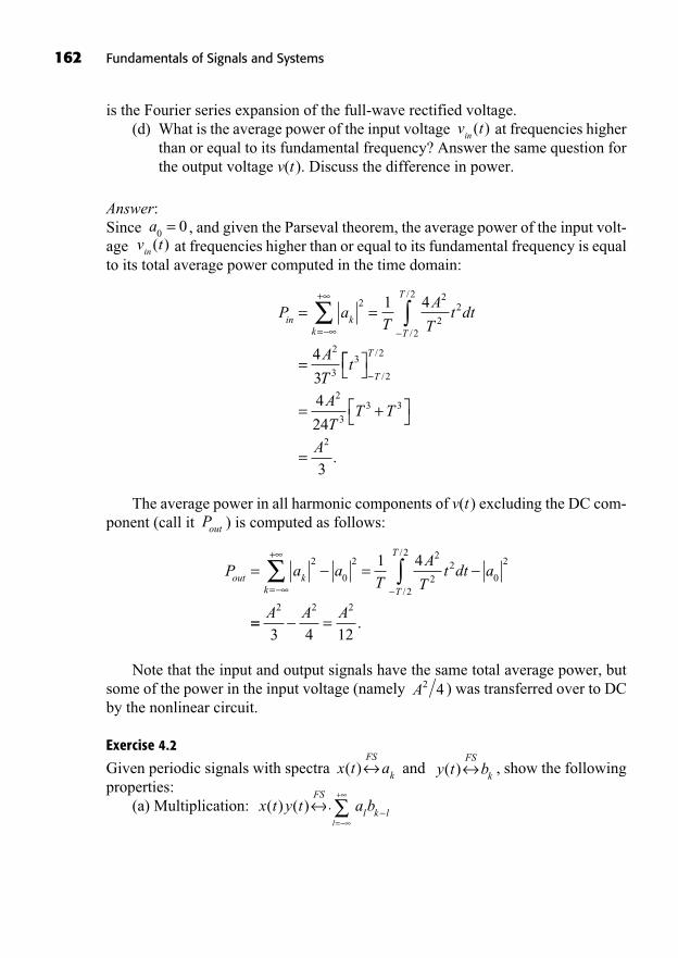
is the Fourier series expansion of the full-wave rectified voltage.(d) What is the average power of the input voltage at frequencies higher
than or equal to its fundamental frequency? Answer the same question forthe output voltage v(t ). Discuss the difference in power.
Answer:Since , and given the Parseval theorem, the average power of the input volt-age at frequencies higher than or equal to its fundamental frequency is equalto its total average power computed in the time domain:
The average power in all harmonic components of v(t ) excluding the DC com-ponent (call it ) is computed as follows:
Note that the input and output signals have the same total average power, butsome of the power in the input voltage (namely ) was transferred over to DCby the nonlinear circuit.
Exercise 4.2
Given periodic signals with spectra and , show the followingproperties:
(a) Multiplication: a bl k ll=
+
x t y tFS
( ) ( )
y t bFS
k( )x t aFS
k( )
A2 4
P a aT
A
Tt dt aout k
k T
T
= ==
+2
0
22
22
2
2
0
21 4
/
/
== =A A A2 2 2
3 4 12.
Pout
P aT
A
Tt dt
A
Tt
in kk T
T
= =
=
=
+2
2
22
2
2
2
33
1 4
4
3
/
/
= +
=
T
T
A
TT T
A
/
/
.
2
2
2
33 3
2
4
24
3
v tin
( )a0 0=
v tin
( )
162 Fundamentals of Signals and Systems
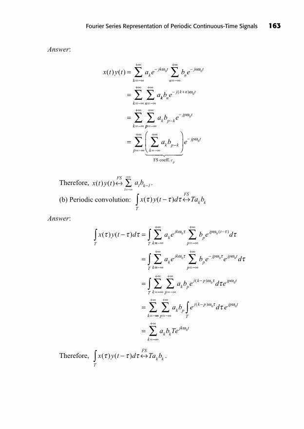
Answer:
Therefore, .
(b) Periodic convolution:
Answer:
Therefore, .x y t d Ta bT
FS
k k( ) ( )
x y t d a e b eT
kjk
pjp t
pk
( ) ( ) ( )==
+0 0
==
+
=
+
=
d
a e b e e
T
kjk
pjp
p
jp t
k
0 0 0
==
+
=
+
=
=
d
a b e d e
T
k pj k p
p
jp t
k
( ) 0 0
+
=
+
=
=
T
k pj k p
Tp
jp t
k
a b e d e( ) 0 0
+
=
+
= a b Tek kjk t
k
0
x y t d Ta bT
FS
k k( ) ( )
a bl k ll=
+
x t y tFS
( ) ( )
x t y t a e b e
a
kjk t
kn
jn t
n
( ) ( ) =
=
=
+
=
+0 0
kk nj k n t
nk
k p kjp t
b e
a b e
+
=
+
=
+
=
( ) 0
0
ppk
k p kk
a b
=
+
=
+
=
+
=
FS coeff.. c
jp t
p
p
e
� ��� ���=
+0
Fourier Series Representation of Periodic Continuous-Time Signals 163
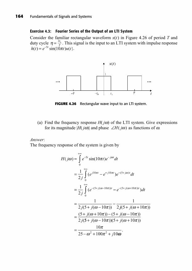
Exercise 4.3: Fourier Series of the Output of an LTI System
Consider the familiar rectangular waveform x(t ) in Figure 4.26 of period T andduty cycle . This signal is the input to an LTI system with impulse response
.h t e t u tt( ) sin( ) ( )= 5 10
20
t
T=
164 Fundamentals of Signals and Systems
FIGURE 4.26 Rectangular wave input to an LTI system.
(a) Find the frequency response H( j ) of the LTI system. Give expressionsfor its magnitude |H( j )| and phase as functions of .
Answer:The frequency response of the system is given by
H j e t e dt
je e
t j t
j t
( ) sin( )
(
=
=
+5
0
10
10
12
++
+=
j t j t
j t
e dt
je
10 5
0
5 1012
)
(
( )
( ( ))
=+
+ ++
e dt
j j
j t( ( )) )
( ( ))
5 10
0
12 5 10
12 jj j
j jj
( ( ))
( ( )) ( ( ))(
5 10
5 10 5 102
+ +
= + + +55 10 5 10
10
25 100 102 2
+ + +
=+ +
j j
j
( ))( ( ))
.
H j( )
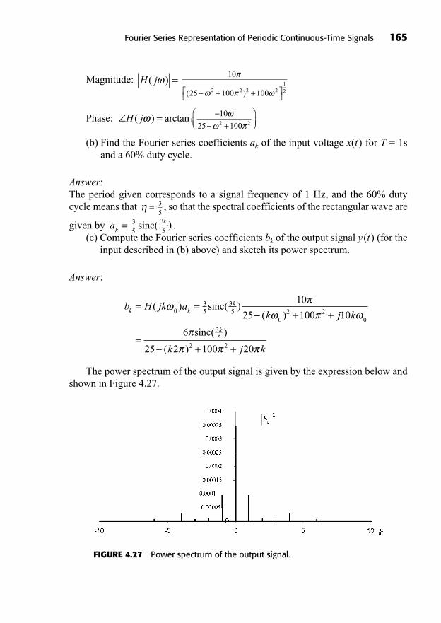
Magnitude:
Phase:
(b) Find the Fourier series coefficients ak of the input voltage x(t ) for T = 1sand a 60% duty cycle.
Answer:The period given corresponds to a signal frequency of 1 Hz, and the 60% dutycycle means that , so that the spectral coefficients of the rectangular wave are
given by .(c) Compute the Fourier series coefficients bk of the output signal y (t ) (for the
input described in (b) above) and sketch its power spectrum.
Answer:
The power spectrum of the output signal is given by the expression below andshown in Figure 4.27.
b H jk akk k
k= =+ +
( ) ( )( )0
35
35
02 2
10
25 100sinc
jj k
k j k
k
10
6
25 2 100 20
0
35
2 2=
+ +sinc( )
( )
)k35
(sinc(35
ak =
= 35
=
+n
10
25 1002 2=H j( ) arctan
( )+ +
10
25 100 1002 2 2 212
H j( ) =
Fourier Series Representation of Periodic Continuous-Time Signals 165
FIGURE 4.27 Power spectrum of the output signal.
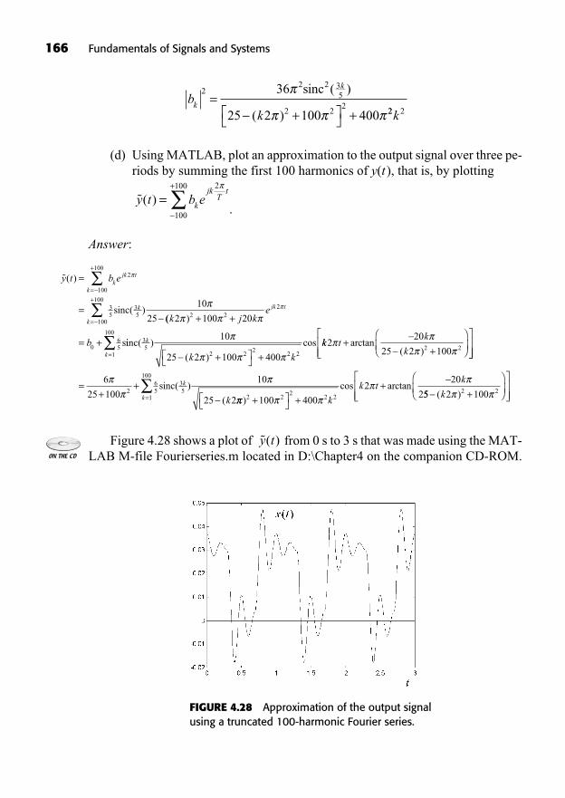
166 Fundamentals of Signals and Systems
(d) Using MATLAB, plot an approximation to the output signal over three pe-riods by summing the first 100 harmonics of y(t ), that is, by plotting
.
Answer:
Figure 4.28 shows a plot of from 0 s to 3 s that was made using the MAT-LAB M-file Fourierseries.m located in D:\Chapter4 on the companion CD-ROM.
y t( )
y t b ekjk t
k
k
( )
( )
=
=
=
+2
100
100
35
35
10
25sinc
(( )k j ke
b
jk t
k 2 100 202 22
100
100
065
+ +
= +
=
+
siinc( )
( )
cos35
2 22
2 2
10
25 2 100 400
k
k k+ +kk t
k
k2
20
25 2 1002 2+
+arctan
( )
=+
+
=k
k
k
1
100
265
35
6
25 100
10
25 2
sinc( )
( )
cos arctan2 2
22 2100 400
220
2+ ++
k
k tk
55 2 1002 21
100
+= ( )kk
y t b ek
jkT
t( ) =
+ 2
100
100
bk
k
k2
2 35
2 22
36
25 2 100 400=
+ +
sinc2( )
( ) 22 2k
FIGURE 4.28 Approximation of the output signalusing a truncated 100-harmonic Fourier series.
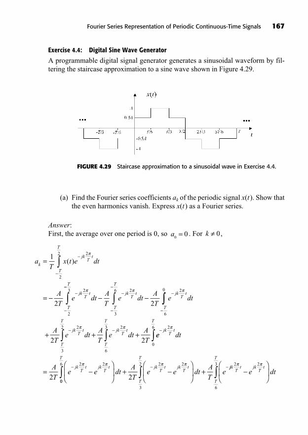
Exercise 4.4: Digital Sine Wave Generator
A programmable digital signal generator generates a sinusoidal waveform by fil-tering the staircase approximation to a sine wave shown in Figure 4.29.
Fourier Series Representation of Periodic Continuous-Time Signals 167
FIGURE 4.29 Staircase approximation to a sinusoidal wave in Exercise 4.4.
(a) Find the Fourier series coefficients ak of the periodic signal x(t). Show thatthe even harmonics vanish. Express x(t ) as a Fourier series.
Answer:First, the average over one period is 0, so . For ,
aT
x t e dt
AT
e dt
k
jkT
t
T
T
jkT
t
T
=
=
1
2
2
2
2
2
2
( )
T
jkT
t
T
T
jkT
t
T
AT
e dtAT
e dt3 2
3
6 2
6
0
2
+ + +AT
e dtAT
e dtAT
jkT
t
T
T
jkT
t
T
T
2 2
2
3
2 2
6
3
ee dt
AT
e e dt
jkT
t
T
jkT
t jkT
t=
2
0
6
2 2
200
6 2 2
3
2
2
T
jkT
t jkT
t
T
T
AT
e e dtAT
e+ +jjk
Tt jk
Tt
T
T
e dt2 2
6
3
k 0a0
0=
168 Fundamentals of Signals and Systems
Note that the coefficients are purely imaginary, which is consistent with ourreal, odd signal. The even spectral coefficients are for:
Figure 4.30 shows a plot of x(t) computed using 250 harmonics in the MAT-LAB program Fourierseries.m, which can be found in the Chapter 4 folder on thecompanion CD-ROM.
The Fourier series representation of x(t ) is
(b) Write x(t ) using the real form of the Fourier series.
x t a B k t C k tk k
k
( ) [ cos( ) sin( )]= +=
+
0 0 01
2
x t a ejA
kkk
jkT
t
k
( ) cos co= = +=
+ 2
2 3ss cosk k e
jkT
t
kk
23
12
0
+ ( )=
+
.
a ajA
mm mk m= = +2 2 2
23
43
1cos cos ++ ( )
= + +
cos
cos co
m
jAm
m m
2
2 2 3ss
cos cos
m m
jAm
m
3
2 2 3
+
= mm m3
0( ) =cos
jAT
kT
t2= sin dt
j AT
kT
t dtjAT
T
T
T
0
6
6
32 2sin sinn
cos
kT
t dt
jAT
Tk
kT
t
T
T
2
22
3
2
= + +0
6
6
322
2T
T
T
j AT
Tk
kT
tcosjjAT
Tk
kT
t
jAk
k
T
T
22
2
3
2
=
cos
cos33
1 223
23
+ +cos cos cosk k kk k
jAk
k
( )
=
cos
cos
23
2 3+ + ( )cos cos .k k
23
1
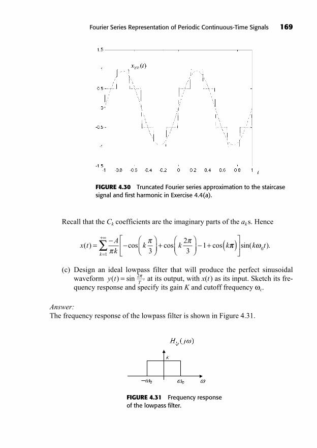
Recall that the Ck coefficients are the imaginary parts of the aks. Hence
(c) Design an ideal lowpass filter that will produce the perfect sinusoidalwaveform at its output, with x(t ) as its input. Sketch its fre-quency response and specify its gain K and cutoff frequency c.
Answer:The frequency response of the lowpass filter is shown in Figure 4.31.
Tt
2y t( ) sin=
x tAk
k k k( ) cos cos cos= + +3
23
1 ( )=
+
sin( ).k tk
01
Fourier Series Representation of Periodic Continuous-Time Signals 169
FIGURE 4.30 Truncated Fourier series approximation to the staircasesignal and first harmonic in Exercise 4.4(a).
FIGURE 4.31 Frequency responseof the lowpass filter.
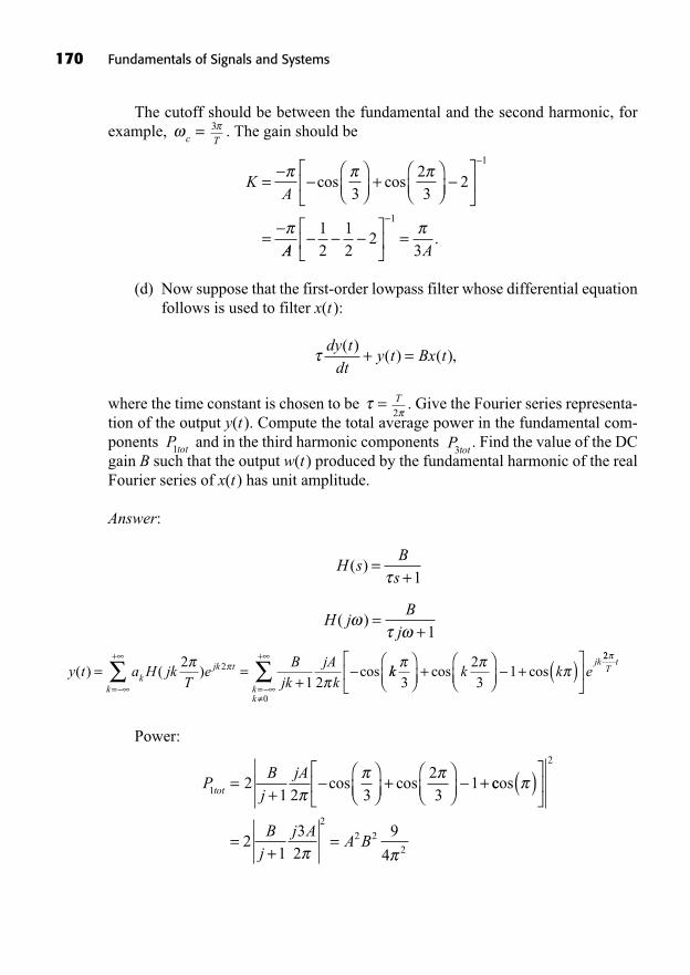
The cutoff should be between the fundamental and the second harmonic, forexample, . The gain should be
(d) Now suppose that the first-order lowpass filter whose differential equationfollows is used to filter x(t ):
where the time constant is chosen to be . Give the Fourier series representa-tion of the output y(t ). Compute the total average power in the fundamental com-ponents and in the third harmonic components . Find the value of the DCgain B such that the output w(t ) produced by the fundamental harmonic of the realFourier series of x(t) has unit amplitude.
Answer:
Power:
PB
jjA
tot1 21 2 3
23
1=+
+ +cos cos ccos( )
=+
=
2
2
2 22
21
32
9
4
Bj
j AA B
y t a H jkT
eB
jkjA
kkjk t
k
( ) ( ) cos= =+=
+ 21 2
2 kk k k ejk
323
1+ + ( )cos cos22
0
Tt
kk=
+
H jB
j( ) =
+1
H sB
s( ) =
+1
P tot3Ptot1
T2
=
dy tdt
y t Bx t( )
( ) ( ),+ =
KA
= +
=
cos cos3
23
2
1
AA A=1
212
23
1
.
T3
c =
170 Fundamentals of Signals and Systems
Fourier Series Representation of Periodic Continuous-Time Signals 171
For the filter’s DC gain B, we found that the gain at 0 should be
Exercises
Exercise 4.5
The output voltage of a half-wave rectifier is given by .
Suppose that the periodic input voltage signal is .Find the fundamental period T and the fundamental frequency 0 of the half-waverectified voltage signal v(t ). Compute the Fourier series coefficients of v(t ) andwrite the voltage as a Fourier series.
Answer:
Exercise 4.6
Suppose that the voltages in the full-wave bridge rectifier circuit of Figure 4.21 are, and . Let be the fundamen-
tal period of the rectified voltage signal v(t ) and let be its fundamentalfrequency.
(a) Compute the Fourier series coefficients of v(t ) and write v(t ) as a Fourierseries.
(b) Express v(t ) as a real Fourier series of the form
2 .B k t C k tk k
[ cos( ) sin( )]1 1
k=
+
1
2
v t a( ) = +0
1 12= T
T T1
2=v t v tin
( ) ( )=v t A t Tin
( ) sin( ),= =0 0
2
v t A t Tin ( ) sin( ),= =1 1 12
v t v t
v tin in
in
( ), ( )
, ( )
> 0
0 0v t( ) =
3 1 1
1
3
00
0
2
0
2
AH j
B
j
B
BA
= =+
=( ) +
=( ) +
( )
.
PB
jjA
tot3 23 1 2
2 1 3=+ ( )+ ( ) + ( )cos cos cos
=+
= =
2
2 2 2
2
2 2
22
3 1 22 2
4
40 5
Bj
jA A B A B
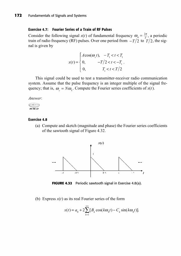
172 Fundamentals of Signals and Systems
Exercise 4.7: Fourier Series of a Train of RF Pulses
Consider the following signal x(t ) of fundamental frequency , a periodictrain of radio frequency (RF) pulses. Over one period from to , the sig-nal is given by
This signal could be used to test a transmitter-receiver radio communicationsystem. Assume that the pulse frequency is an integer multiple of the signal fre-quency; that is, . Compute the Fourier series coefficients of x(t ).
Answer:
Exercise 4.8
(a) Compute and sketch (magnitude and phase) the Fourier series coefficientsof the sawtooth signal of Figure 4.32.
cN=
0
x t
A t T t T
T t T
T t T
c
( )
cos( ),
,
,
=< <
< << <
1 1
1
1
0 2
0 2
.
T 2T 2
2
T0=
FIGURE 4.32 Periodic sawtooth signal in Exercise 4.8(a).
(b) Express x(t ) as its real Fourier series of the form
x t a B k t C k tk k
k
( ) [ cos( ) sin( )].= +=
+
0 0 01
2
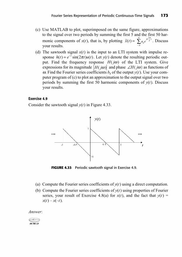
(c) Use MATLAB to plot, superimposed on the same figure, approximationsto the signal over two periods by summing the first 5 and the first 50 har-
monic components of x(t ), that is, by plotting . Discussyour results.
(d) The sawtooth signal x(t ) is the input to an LTI system with impulse re-sponse . Let y(t ) denote the resulting periodic out-put. Find the frequency response of the LTI system. Giveexpressions for its magnitude and phase as functions of
. Find the Fourier series coefficients bk of the output y(t ). Use your com-puter program of (c) to plot an approximation to the output signal over twoperiods by summing the first 50 harmonic components of y(t ). Discussyour results.
Exercise 4.9
Consider the sawtooth signal y(t ) in Figure 4.33.
H j( )H j( )H j( )
h t e t u tt( ) sin( ) ( )= 2
a ek
jkT
t
N
N 2
x t( ) =
Fourier Series Representation of Periodic Continuous-Time Signals 173
FIGURE 4.33 Periodic sawtooth signal in Exercise 4.9.
(a) Compute the Fourier series coefficients of y(t ) using a direct computation.
(b) Compute the Fourier series coefficients of y(t ) using properties of Fourierseries, your result of Exercise 4.8(a) for x(t ), and the fact that y(t ) =x(t ) – x(–t).
Answer:

Exercise 4.10
Compute and sketch (magnitude and phase) the Fourier series coefficients of thefollowing signals:
(a) Signal x(t ) shown in Figure 4.34.
(b) x t t t( ) sin( ) cos( )= +10 20
174 Fundamentals of Signals and Systems
FIGURE 4.34 Periodic rectangular signal in Exercise 4.10(a).
175
The Continuous-TimeFourier Transform
5
In This Chapter
Fourier Transform as the Limit of a Fourier SeriesProperties of the Fourier TransformExamples of Fourier TransformsThe Inverse Fourier TransformDualityConvergence of the Fourier TransformThe Convolution Property in the Analysis of LTI SystemsFourier Transforms of Periodic SignalsFilteringSummaryTo Probe FurtherExercises
((Lecture 15: Definition and Properties of the Continuous-Time Fourier Transform))
The Fourier series is a frequency-domain representation of a continuous-timeperiodic signal. What about aperiodic signals? The concept of Fourier seriescan be extended to the Fourier transform, which applies to many aperiodic
signals. For instance, all signals of finite energy have a Fourier transform, alsocalled a spectrum.
As mentioned earlier, engineers often like to think of a signal as a spectrumwhose energy is mostly contained in certain frequency bands. For instance, the
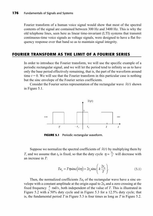
176 Fundamentals of Signals and Systems
Fourier transform of a human voice signal would show that most of the spectralcontents of the signal are contained between 300 Hz and 3400 Hz. This is why theold telephone lines, seen here as linear time-invariant (LTI) systems that transmitcontinuous-time voice signals as voltage signals, were designed to have a flat fre-quency response over that band so as to maintain signal integrity.
FOURIER TRANSFORM AS THE LIMIT OF A FOURIER SERIES
In order to introduce the Fourier transform, we will use the specific example of aperiodic rectangular signal, and we will let the period tend to infinity so as to haveonly the base period effectively remaining, that is, the part of the waveform aroundtime t = 0. We will see that the Fourier transform in this particular case is nothingbut the sinc envelope of the Fourier series coefficients.
Consider the Fourier series representation of the rectangular wave shownin Figure 5.1.
x t( )
FIGURE 5.1 Periodic rectangular waveform.
Suppose we normalize the spectral coefficients of by multiplying them byT, and we assume that t0 is fixed, so that the duty cycle will decrease withan increase in T:
(5.1)
Then, the normalized coefficients Tak of the rectangular wave have a sinc en-velope with a constant amplitude at the origin equal to 2t0 and a zero crossing at thefixed frequency , both independent of the value of T. This is illustrated inFigure 5.2 with a 50% duty cycle and in Figure 5.3 for a 12.5% duty cycle; that is, the fundamental period T in Figure 5.3 is four times as long as T in Figure 5.2.
rad/st0
Ta T k t kt
Tk= ( ) =sinc sinc2
20
0 .
20
t
T=
x t( )
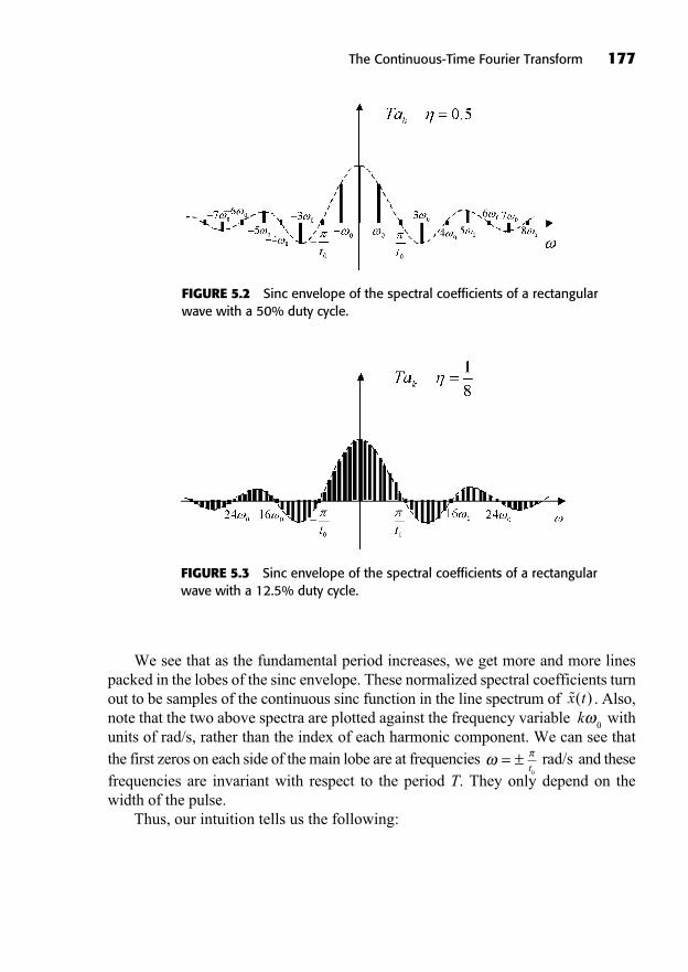
We see that as the fundamental period increases, we get more and more linespacked in the lobes of the sinc envelope. These normalized spectral coefficients turnout to be samples of the continuous sinc function in the line spectrum of . Also,note that the two above spectra are plotted against the frequency variable withunits of rad/s, rather than the index of each harmonic component. We can see that the first zeros on each side of the main lobe are at frequencies and these frequencies are invariant with respect to the period T. They only depend on thewidth of the pulse.
Thus, our intuition tells us the following:
rad/st0
= ±
k0
x t( )
The Continuous-Time Fourier Transform 177
FIGURE 5.2 Sinc envelope of the spectral coefficients of a rectangularwave with a 50% duty cycle.
FIGURE 5.3 Sinc envelope of the spectral coefficients of a rectangularwave with a 12.5% duty cycle.
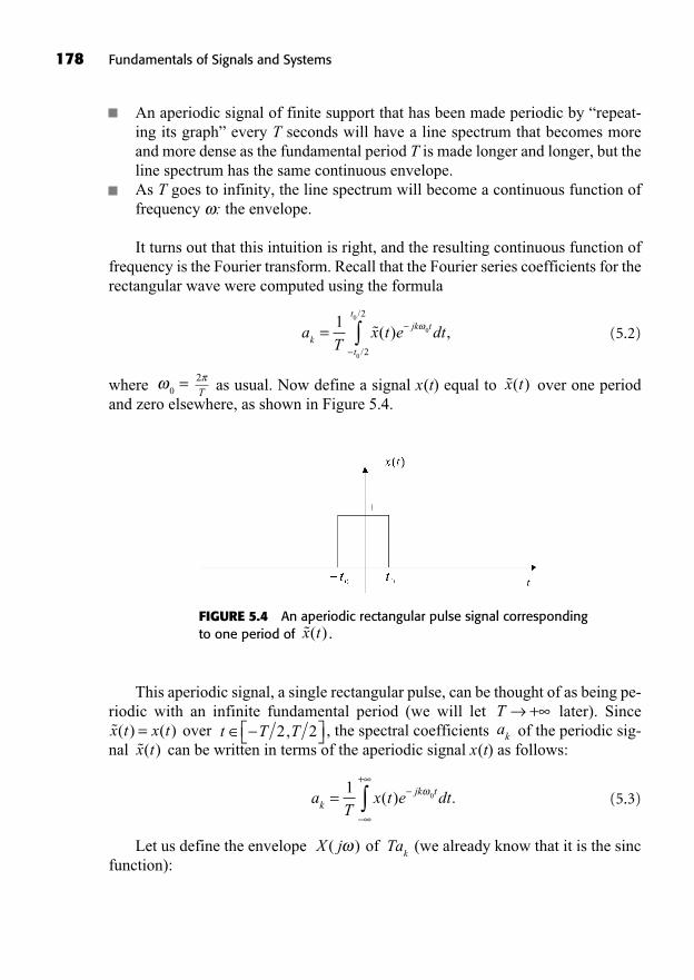
178 Fundamentals of Signals and Systems
An aperiodic signal of finite support that has been made periodic by “repeat-ing its graph” every T seconds will have a line spectrum that becomes moreand more dense as the fundamental period T is made longer and longer, but theline spectrum has the same continuous envelope.As T goes to infinity, the line spectrum will become a continuous function offrequency : the envelope.
It turns out that this intuition is right, and the resulting continuous function offrequency is the Fourier transform. Recall that the Fourier series coefficients for therectangular wave were computed using the formula
(5.2)
where as usual. Now define a signal x(t) equal to over one periodand zero elsewhere, as shown in Figure 5.4.
x t( )2
T0=
aT
x t e dtk
jk t
t
t
=1
0
0
0
2
2
( ) ,/
/
FIGURE 5.4 An aperiodic rectangular pulse signal correspondingto one period of . x t( )
This aperiodic signal, a single rectangular pulse, can be thought of as being pe-riodic with an infinite fundamental period (we will let later). Since
over , the spectral coefficients of the periodic sig-nal can be written in terms of the aperiodic signal x(t) as follows:
(5.3)
Let us define the envelope of (we already know that it is the sincfunction):
Tak
X j( )
aT
x t e dtkjk t=
+1
0( ) .
x t( )akt T T2 2, x t x t( ) ( )=T +
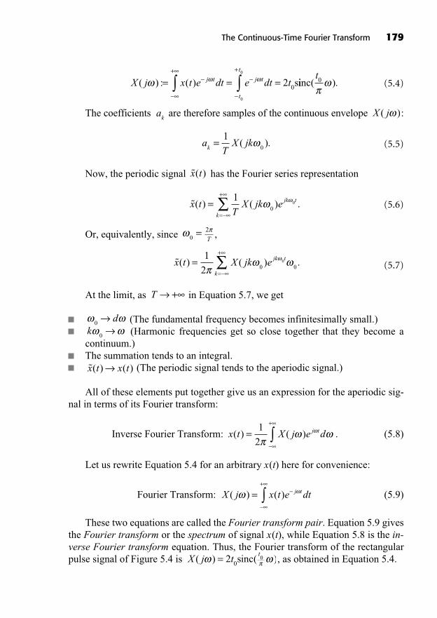
(5.4)
The coefficients are therefore samples of the continuous envelope :
(5.5)
Now, the periodic signal has the Fourier series representation
(5.6)
Or, equivalently, since ,
(5.7)
At the limit, as in Equation 5.7, we get
(The fundamental frequency becomes infinitesimally small.)(Harmonic frequencies get so close together that they become a
continuum.)The summation tends to an integral.
(The periodic signal tends to the aperiodic signal.)
All of these elements put together give us an expression for the aperiodic sig-nal in terms of its Fourier transform:
Inverse Fourier Transform: . (5.8)
Let us rewrite Equation 5.4 for an arbitrary x(t) here for convenience:
Fourier Transform: (5.9)
These two equations are called the Fourier transform pair. Equation 5.9 givesthe Fourier transform or the spectrum of signal x(t), while Equation 5.8 is the in-verse Fourier transform equation. Thus, the Fourier transform of the rectangularpulse signal of Figure 5.4 is , as obtained in Equation 5.4.X j t
t( ) ( )= 2 0
0sinc
X j x t e dtj t( ) ( )=+
x t X j e dj t( ) ( )=+1
2
x t x t( ) ( )
k0
0d
T +
x t X jk e jk t
k
( ) ( ) .==
+1
2 0 00
2
T0=
x tT
X jk e jk t
k
( ) ( ) .==
+ 10
0
x t( )
aT
X jkk=
10
( ).
X j( )ak
X j x t e dt e dt tj t j t
t
t
( ) : ( )= = =+ +
0
0
2 0siinc( ).t0
The Continuous-Time Fourier Transform 179
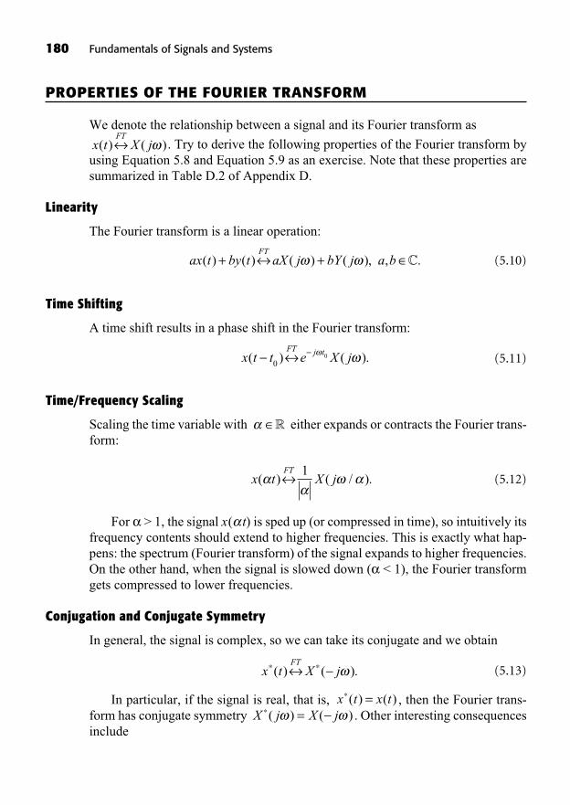
PROPERTIES OF THE FOURIER TRANSFORM
We denote the relationship between a signal and its Fourier transform as
. Try to derive the following properties of the Fourier transform byusing Equation 5.8 and Equation 5.9 as an exercise. Note that these properties aresummarized in Table D.2 of Appendix D.
Linearity
The Fourier transform is a linear operation:
(5.10)
Time Shifting
A time shift results in a phase shift in the Fourier transform:
(5.11)
Time/Frequency Scaling
Scaling the time variable with either expands or contracts the Fourier trans-form:
(5.12)
For > 1, the signal x( t) is sped up (or compressed in time), so intuitively itsfrequency contents should extend to higher frequencies. This is exactly what hap-pens: the spectrum (Fourier transform) of the signal expands to higher frequencies.On the other hand, when the signal is slowed down ( < 1), the Fourier transformgets compressed to lower frequencies.
Conjugation and Conjugate Symmetry
In general, the signal is complex, so we can take its conjugate and we obtain
(5.13)
In particular, if the signal is real, that is, , then the Fourier trans-form has conjugate symmetry . Other interesting consequencesinclude
X j X j=( ) ( )x t x t=( ) ( )
x t X jFT
( ) ( ).
x t X jFT
( ) ( / ).1
�
x t t e X jFT j t( ) ( ).0
0
ax t by t aX j bY j a bFT
( ) ( ) ( ) ( ), , .+ + �
x t X jFT
( ) ( )
180 Fundamentals of Signals and Systems

, an even function of , an odd function of
, an even function of , an odd function of
Furthermore, if is real and even, then we can show that, that is, the spectrum is even and real.
Similarly, if x(t) is real and odd, we have, that is, the spectrum is odd and purely
imaginary.
Differentiation
Differentiating a signal results in a multiplication of the Fourier transform by j :
(5.14)
Integration
Integration of a signal results in a division of the Fourier transform by j . How-ever, to account for the possibility that x(t) has a nonzero, but finite, average value,
that is, , we must add the term to the
Fourier transform. That is, upon integrating x(t), the nonzero average value of x(t)produces a constant part with finite power concentrated at DC ( = 0), and this isrepresented as an impulse at that frequency.
(5.15)
Convolution
The convolution of two signals results in the multiplication of their Fourier trans-forms in the frequency domain:
(5.16)
A direct application of this property is the calculation of the response of an LTIsystem with impulse response h(t) to an arbitrary input signal x(t), which is givenby the convolution . The Fourier transform of the output Y( j ) isobtained by multiplying the Fourier transform of the input signal X( j ) with the
y t x t h t( ) ( ) ( )=
x t y t X j Y jFT
( ) ( ) ( ) ( ).
x dj
X j Xt
FT( ) ( ) ( ) ( ).+1
0
X ( ) ( )0x t dt( ) 0=+
X j X( ) ( )0 0= =
ddt
x t j X jFT
( ) ( ).
X j X j X j( ) ( ) ( )= =
X j X j X j( ) ( ) ( )= =x t( )
=X j X j( ) ( )| ( ) | | ( ) |X j X j=Im{ ( )} Im{ ( )}X j X j=Re{ ( )} Re{ ( )}X j X j=
The Continuous-Time Fourier Transform 181
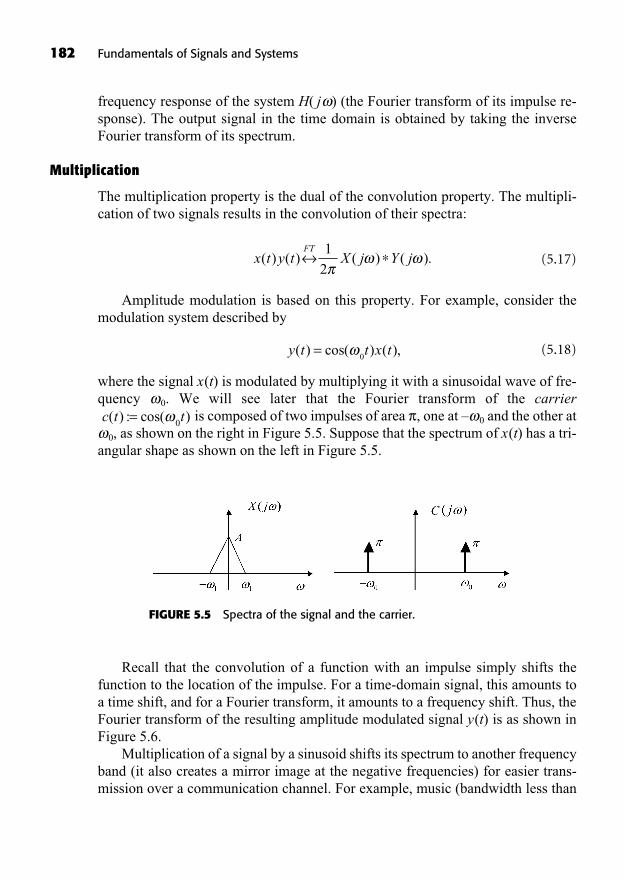
182 Fundamentals of Signals and Systems
frequency response of the system H( j ) (the Fourier transform of its impulse re-sponse). The output signal in the time domain is obtained by taking the inverseFourier transform of its spectrum.
Multiplication
The multiplication property is the dual of the convolution property. The multipli-cation of two signals results in the convolution of their spectra:
(5.17)
Amplitude modulation is based on this property. For example, consider themodulation system described by
(5.18)
where the signal x(t) is modulated by multiplying it with a sinusoidal wave of fre-quency 0. We will see later that the Fourier transform of the carrier
is composed of two impulses of area , one at – 0 and the other at0, as shown on the right in Figure 5.5. Suppose that the spectrum of x(t) has a tri-
angular shape as shown on the left in Figure 5.5.
c t t( ) : cos( )= 0
y t t x t( ) cos( ) ( ),=0
x t y t X j Y jFT
( ) ( ) ( ) ( ).1
2
FIGURE 5.5 Spectra of the signal and the carrier.
Recall that the convolution of a function with an impulse simply shifts thefunction to the location of the impulse. For a time-domain signal, this amounts toa time shift, and for a Fourier transform, it amounts to a frequency shift. Thus, theFourier transform of the resulting amplitude modulated signal y(t) is as shown inFigure 5.6.
Multiplication of a signal by a sinusoid shifts its spectrum to another frequencyband (it also creates a mirror image at the negative frequencies) for easier trans-mission over a communication channel. For example, music (bandwidth less than

20 kHz) transmitted over typical AM radio has modulation frequencies in the rangeof 500 kHz to 1500 kHz. Modulated signals in this range can be convenientlytransmitted at reasonable power by using “reasonable size” antennas (actually theyseem large by today’s standards!). The basic theory of modulation is presented inChapter 16.
Energy-Density Spectrum
Recall that the power spectrum of a periodic signal is defined as the squared mag-nitudes of its Fourier series coefficients. A plot of the power spectrum of a signalgives us an idea of the density of power at different frequencies (harmonics).
Similarly, the energy-density spectrum of an aperiodic signal is defined as the magnitude squared of its spectrum; that is, is the energy-density spec-trum of x(t). We can find the energy of a signal in a given frequency band by inte-grating its energy-density spectrum over the interval of frequencies.
For example,
(5.19)
Note that for real signals, it is customary to include the negative frequencyband as well. For example, if we wanted to compute the energy contained in a realsignal between, for example, 5 kHz and 10 kHz, we would compute
(5.20)E X j dr[ , ] ( )10000 20000
2
10000
200001
2= + XX j d X j d( ) ( )
2
20000
1000021=
110000
20000
E X j da b
a
b
[ , ] : ( ) .= 12
2
X j( )2
The Continuous-Time Fourier Transform 183
FIGURE 5.6 Spectrum of an amplitude modulated signal.
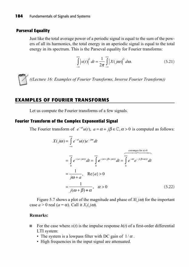
Parseval Equality
Just like the total average power of a periodic signal is equal to the sum of the pow-ers of all its harmonics, the total energy in an aperiodic signal is equal to the totalenergy in its spectrum. This is the Parseval equality for Fourier transforms:
(5.21)
((Lecture 16: Examples of Fourier Transforms, Inverse Fourier Transform))
EXAMPLES OF FOURIER TRANSFORMS
Let us compute the Fourier transforms of a few signals.
Fourier Transform of the Complex Exponential Signal
The Fourier transform of is computed as follows:
(5.22)
Figure 5.7 shows a plot of the magnitude and phase of X( j ) for the importantcase a > 0 real (a = ). Call it X1( j ).
Remarks:
For the case where x(t) is the impulse response h(t) of a first-order differentialLTI system:• The system is a lowpass filter with DC gain of .• High frequencies in the input signal are attenuated.
1/
X j e u t e dt
e dt
at j t
a j t
( ) ( )
( )
=
= =
+
++
0
ee dt e e dtj j t t j t+ ++
++
=( ) ( )
0 0
conveerges for >
=+
>
=+
0
10
1
� ��� ��
j aa
j
, Re{ }
( )++>, 0
e u t a jat = + >( ), ,C 0
x t dt X j d( ) ( ) .2 21
2
+ +
=
184 Fundamentals of Signals and Systems
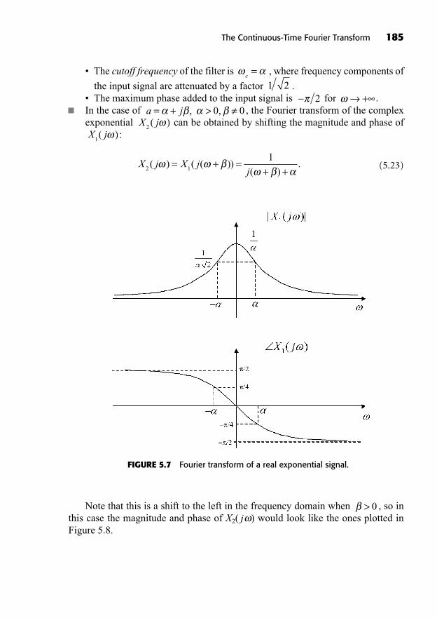
The Continuous-Time Fourier Transform 185
• The cutoff frequency of the filter is , where frequency components of
the input signal are attenuated by a factor .• The maximum phase added to the input signal is for .In the case of , the Fourier transform of the complexexponential can be obtained by shifting the magnitude and phase of
:
(5.23)X j X jj2 1
1( ) ( ( ))
( ).= + =
+ +
X j1( )
X j2( )
a j= + >, ,0 0+2
1 2c=
FIGURE 5.7 Fourier transform of a real exponential signal.
Note that this is a shift to the left in the frequency domain when , so inthis case the magnitude and phase of X2( j ) would look like the ones plotted inFigure 5.8.
> 0
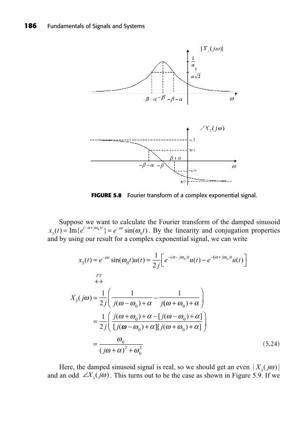
186 Fundamentals of Signals and Systems
Suppose we want to calculate the Fourier transform of the damped sinusoid. By the linearity and conjugation properties
and by using our result for a complex exponential signal, we can write
(5.24)
Here, the damped sinusoid signal is real, so we should get an even and an odd . This turns out to be the case as shown in Figure 5.9. If weX j
3( )
| ( ) |X j3
x t e t u tj
e u t et j t3 0
12
0( ) sin( ) ( ) ( )( )= = (( ) ( )
( )( )
+
=+
j t
FT
u t
X jj j j
0
30
12
1 1(( )
( ) [ ( ) ]
[ (
+ +
=+ + +
0
0 012 j
j j
j + + +
=+ +
0 0
02
02
) ][ ( ) ]
( )
j
j
x t e e tj t t3 0
0( ) Im{ } sin( )( )= =+
FIGURE 5.8 Fourier transform of a complex exponential signal.
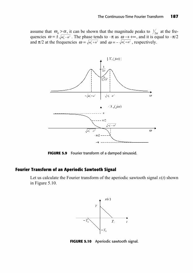
The Continuous-Time Fourier Transform 187
assume that , it can be shown that the magnitude peaks to at the fre-quencies . The phase tends to – as , and it is equal to – /2and /2 at the frequencies and , respectively.+
02 2=+
02 2=
+02 2= ±
120
>
FIGURE 5.9 Fourier transform of a damped sinusoid.
Fourier Transform of an Aperiodic Sawtooth Signal
Let us calculate the Fourier transform of the aperiodic sawtooth signal x(t) shownin Figure 5.10.
FIGURE 5.10 Aperiodic sawtooth signal.
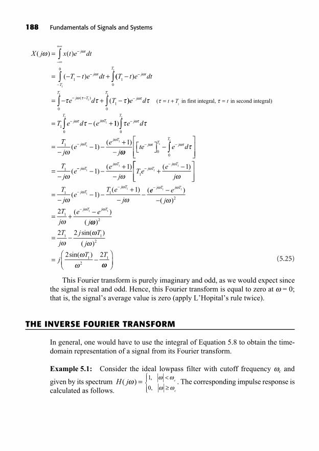
(5.25)
This Fourier transform is purely imaginary and odd, as we would expect sincethe signal is real and odd. Hence, this Fourier transform is equal to zero at = 0;that is, the signal’s average value is zero (apply L’Hopital’s rule twice).
THE INVERSE FOURIER TRANSFORM
In general, one would have to use the integral of Equation 5.8 to obtain the time-domain representation of a signal from its Fourier transform.
Example 5.1: Consider the ideal lowpass filter with cutoff frequency c and
given by its spectrum . The corresponding impulse response iscalculated as follows.
c
c
,
,
<1
0H j( ) =
X j x t e dt
T t e dt
j t
j t
T
( ) ( )
( )
=
= +
+
1
0
1
(( )
(( )
T t e dt
e d T
j t
T
j TT
10
01
1
1
1
= + )) (e dj
T
t T t= + =0
1
1 in first integral, in second integral)
= +T e d ej
Tj T
10
1
1( 11
11
0
1
1
1
1
)
( )( )
e d
T
je
e
j
j
T
j Tj T
=+
te e d
T
je
j tT
j
T
=
00
1
11
(+
+j Tj T
j Tj Te
jT e
e
j1
1
1
1
11 1
1)
( ) ( )
=+T
je
T e
jj T
j T
1 11
1
11
( )( ) (ee e
j
T
j
e e
j
j T j T
j T j T
= +
1 1
1 1
2
12
)
( )
( )
( )
sin( )
( )
sin( )
2
1 12
12
1
2 2
2 2
=
=
T
j
j T
j
jT T
188 Fundamentals of Signals and Systems
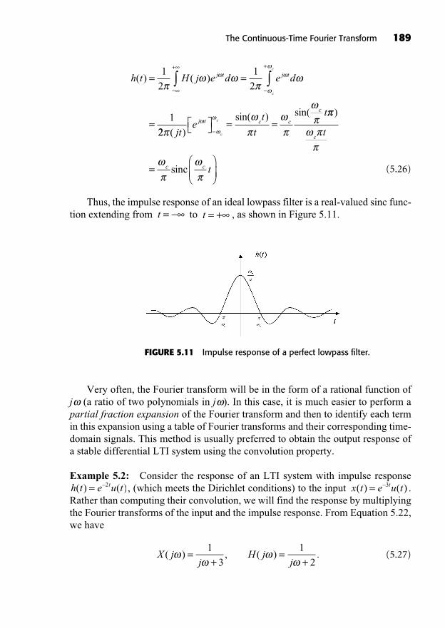
The Continuous-Time Fourier Transform 189
(5.26)
Thus, the impulse response of an ideal lowpass filter is a real-valued sinc func-tion extending from to , as shown in Figure 5.11.t = +t =
h t H j e d e dj t j t
c
c
( ) ( )= =
=
+ +1
2
1
2
1
22 ( )
sin( ) sin(
jte
t
t
tj t c c
c
c
c = =)
c
c c
t
t= sinc
FIGURE 5.11 Impulse response of a perfect lowpass filter.
Very often, the Fourier transform will be in the form of a rational function ofj (a ratio of two polynomials in j ). In this case, it is much easier to perform apartial fraction expansion of the Fourier transform and then to identify each termin this expansion using a table of Fourier transforms and their corresponding time-domain signals. This method is usually preferred to obtain the output response ofa stable differential LTI system using the convolution property.
Example 5.2: Consider the response of an LTI system with impulse response , (which meets the Dirichlet conditions) to the input .
Rather than computing their convolution, we will find the response by multiplyingthe Fourier transforms of the input and the impulse response. From Equation 5.22,we have
(5.27)X jj
H jj
( ) , ( ) .=+
=+
1
3
1
2
x t e u tt( ) ( )= 3h t e u tt( ) ( )= 2
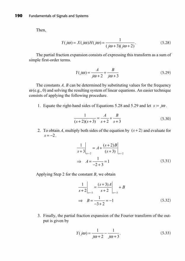
190 Fundamentals of Signals and Systems
Then,
(5.28)
The partial fraction expansion consists of expressing this transform as a sum ofsimple first-order terms.
(5.29)
The constants A, B can be determined by substituting values for the frequency(e.g., 0) and solving the resulting system of linear equations. An easier technique
consists of applying the following procedure.
1. Equate the right-hand sides of Equations 5.28 and 5.29 and let .
(5.30)
2. To obtain A, multiply both sides of the equation by and evaluate for.
(5.31)
Applying Step 2 for the constant B, we obtain
(5.32)
3. Finally, the partial fraction expansion of the Fourier transform of the out-put is given by
(5.33)Y jj j
( ) .=+ +
1
2
1
3
1
2
3
2
1
3 21
3 3s
s A
sB
B
s s+
=++
+
=+
=
= =
( )
1
3
2
3
1
2 31
2 2s
As B
s
A
s s+
= +++
=+
=
= =
( )
( )
s = 2( )s + 2
1
2 3 2 3( )( )s s
A
s
B
s+ +=
++
+
s j:=
Y jA
j
B
j( ) =
++
+2 3
Y j X j H jj j
( ) ( ) ( )( )( )
.= =+ +
1
3 2
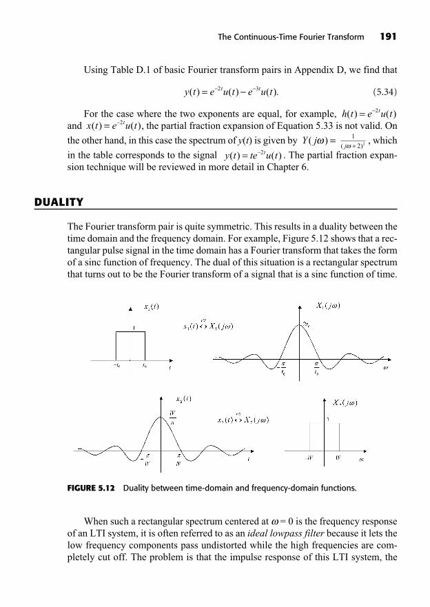
Using Table D.1 of basic Fourier transform pairs in Appendix D, we find that
(5.34)
For the case where the two exponents are equal, for example, and , the partial fraction expansion of Equation 5.33 is not valid. On
the other hand, in this case the spectrum of y(t) is given by , which
in the table corresponds to the signal . The partial fraction expan-sion technique will be reviewed in more detail in Chapter 6.
DUALITY
The Fourier transform pair is quite symmetric. This results in a duality between thetime domain and the frequency domain. For example, Figure 5.12 shows that a rec-tangular pulse signal in the time domain has a Fourier transform that takes the formof a sinc function of frequency. The dual of this situation is a rectangular spectrumthat turns out to be the Fourier transform of a signal that is a sinc function of time.
y t te u tt( ) ( )= 2j( )+
1
2 2Y j( ) =x t e u tt( ) ( )= 2
h t e u tt( ) ( )= 2
y t e u t e u tt t( ) ( ) ( ).= 2 3
The Continuous-Time Fourier Transform 191
FIGURE 5.12 Duality between time-domain and frequency-domain functions.
When such a rectangular spectrum centered at = 0 is the frequency responseof an LTI system, it is often referred to as an ideal lowpass filter because it lets thelow frequency components pass undistorted while the high frequencies are com-pletely cut off. The problem is that the impulse response of this LTI system, the
time-domain sinc function, is noncausal. Filter design will be discussed in more de-tail later on.
((Lecture 17: Convergence of the Fourier Transform, Convolution Property andLTI Systems))
CONVERGENCE OF THE FOURIER TRANSFORM
There are two important classes of signals for which the Fourier transform converges:
1. Signals of finite total energy, that is, signals for which 2. Signals that satisfy the Dirichlet conditions:
a. x(t) is absolutely integrable, that is, .
b. x(t) has a finite number of maxima and minima over any finite intervalof time.
c. x(t) has a finite number of discontinuities over any finite interval oftime. Furthermore, each one of these discontinuities must be finite.
The type of convergence that we get for signals of finite energy is similar to the convergence of Fourier series for signals of finite power. That is, there is no energy in the error between a signal x(t) and its inverse Fourier transform
. For signals x(t) satisfying the Dirichlet conditions, it
is guaranteed that is equal to x(t) at every time t, except at discontinuitieswhere will take on the average of the values on either side of the discontinuity.
Later, we will extend the Fourier transform to include periodic signals (infinite en-ergy, finite power) by allowing the use of impulse functions in the frequency domain.
THE CONVOLUTION PROPERTY IN THE ANALYSIS OF LTI SYSTEMS
General LTI Systems
We have seen that the response of a stable LTI system to a complex exponential of the type is simply the same exponential multiplied by the frequency re-sponse of the system . We used this fact to find the Fourier series co-efficients of the output of an LTI system as the product for aperiodic input of frequency 0 with spectral coefficients ak.
b H jk ak k= ( )
0
H j e j t( )e j t
x t( ) x t( )
X j e dj t( )+1
2 x t( ) =
x t dt( ) < ++
x t dt( )2
< ++
192 Fundamentals of Signals and Systems
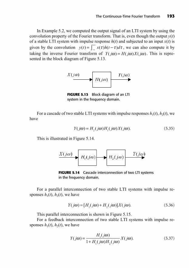
In Example 5.2, we computed the output signal of an LTI system by using theconvolution property of the Fourier transform. That is, even though the output y(t)of a stable LTI system with impulse response h(t) and subjected to an input x(t) isgiven by the convolution , we can also compute it by taking the inverse Fourier transform of . This is repre-sented in the block diagram of Figure 5.13.
Y j H j X j( ) ( ) ( )=x h t d( ) ( )
+y t( ) =
The Continuous-Time Fourier Transform 193
FIGURE 5.13 Block diagram of an LTIsystem in the frequency domain.
For a cascade of two stable LTI systems with impulse responses h1(t), h2(t), wehave
(5.35)
This is illustrated in Figure 5.14.
Y j H j H j X j( ) ( ) ( ) ( ).=2 1
FIGURE 5.14 Cascade interconnection of two LTI systemsin the frequency domain.
For a parallel interconnection of two stable LTI systems with impulse re-sponses h1(t), h2(t), we have
(5.36)
This parallel interconnection is shown in Figure 5.15.For a feedback interconnection of two stable LTI systems with impulse re-
sponses h1(t), h2(t), we have
(5.37)Y jH j
H j H jX j( )
( )
( ) ( )( ).=
+1
1 21
Y j H j H j X j( ) [ ( ) ( )] ( ).= +1 2
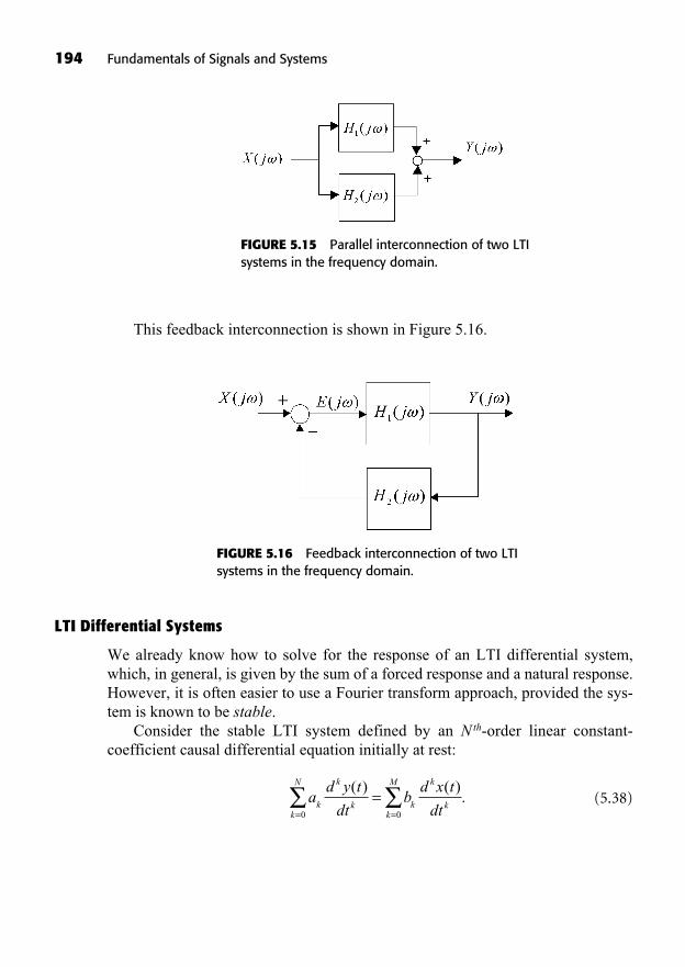
This feedback interconnection is shown in Figure 5.16.
194 Fundamentals of Signals and Systems
FIGURE 5.15 Parallel interconnection of two LTIsystems in the frequency domain.
FIGURE 5.16 Feedback interconnection of two LTIsystems in the frequency domain.
LTI Differential Systems
We already know how to solve for the response of an LTI differential system,which, in general, is given by the sum of a forced response and a natural response.However, it is often easier to use a Fourier transform approach, provided the sys-tem is known to be stable.
Consider the stable LTI system defined by an N th-order linear constant-coefficient causal differential equation initially at rest:
(5.38)ad y t
dtb
d x t
dtk
k
kk
N
k
k
kk
M( ) ( ).
= =
=0 0
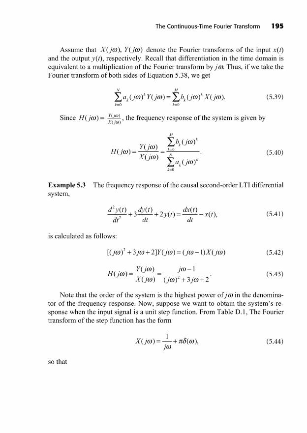
Assume that denote the Fourier transforms of the input x(t)and the output y(t), respectively. Recall that differentiation in the time domain isequivalent to a multiplication of the Fourier transform by j . Thus, if we take theFourier transform of both sides of Equation 5.38, we get
(5.39)
Since , the frequency response of the system is given by
(5.40)
Example 5.3 The frequency response of the causal second-order LTI differential system,
(5.41)
is calculated as follows:
(5.42)
(5.43)
Note that the order of the system is the highest power of j in the denomina-tor of the frequency response. Now, suppose we want to obtain the system’s re-sponse when the input signal is a unit step function. From Table D.1, The Fouriertransform of the step function has the form
(5.44)
so that
X jj
( ) ( ),= +1
H jY j
X j
j
j j( )
( )
( ) ( ).= =
+ +1
3 22
[( ) ] ( ) ( ) ( )j j Y j j X j2 3 2 1+ + =
d y t
dt
dy t
dty t
dx t
dtx t
2
23 2
( ) ( )( )
( )( ),+ + =
H jY j
X j
b j
a j
kk
k
M
kk
k
N( )
( )
( )
( )
( )
.= = =
=
0
0
Y j
X j
( )
( )H j( ) =
a j Y j b j X jk
k
k
N
kk
k
M
( ) ( ) ( ) ( ).= =
=0 0
X j Y j( ), ( )
The Continuous-Time Fourier Transform 195
(5.45)
Letting s = j and expanding the rational function on the right-hand side intopartial fractions, we get
(5.46)
and the coefficients are computed as follows:
(5.47)
(5.48)
(5.49)
Hence,
(5.50)
and using Table D.1 of Fourier transform pairs, we find the output by inspection:
(5.51)y t e e u tt t( ) ( ).= +1
22
3
22
Y jj
j j j
j
( )( )
( )=+ +
= +
1
3 2
1
2
1
2
1
2
( ) ++ +
21
1
3
2
1
2j j
Cs
s ss
=+
==
1
1
3
22
( )
Bs
s ss
=+
= ==
1
2
2
12
1( )
As
s ss
=+ +
==
1
1 2
1
20
( )( )
s
s s s
s
s s s
A
s
B
s
C
s+ +=
+ += +
++
+1
3 2
1
1 2 1 22 ( )( ),,
Y jj
j jX j
j
j j
( )( )
( )
( )
=+ +
=+ +
1
3 2
1
3 2
1
2
2 jj
j
j j j
+
=+ +
( )
( )(
1
3 2
1
22)
sampling property� �� ��
196 Fundamentals of Signals and Systems
Remark: When in differential Equation 5.38, the frequency responsehas a numerator of equal or higher order than the denominator polynomial. It isthen necessary to express the frequency response as a sum of a strictly properrational function (it means that the numerator polynomial is of lower order than thedenominator) and a polynomial in j of order . Each term of this polyno-mial is associated either with an impulse (constant term), a doublet (term in j ), ora k th-order derivative of the impulse (term in ( j )k). Then, one only needs to per-form a partial fraction expansion of the resulting strictly proper rational function tofind the other time-domain components of the response.
((Lecture 18: LTI Systems, Fourier Transform of Periodic Signals))
Example 5.4: Consider the causal LTI differential system initially at rest de-scribed by
(5.52)
The frequency response of this system is
(5.53)
Let s = j and write H(s) as
(5.54)
Multiplying both sides by 2(s + 0.5), we can identify each coefficient:
(5.55)
, , . (5.56)
Thus,
(5.57)H ss s
ss
s( )
( . ) ( . )=
+=
+
2 2
2 0 5
1
2
3
4
5
8
1
0 5
C =5
8B =
3
4A =
1
2
s s s As B C As A B s C B2 22 2 0 5 2 2 2 2= + + + = + + + +( . )( ) ( )
H ss s
sAs B
C
s( )
( . ) ( . )=
+= + +
+
2 2
2 0 5 0 5
H jj j
j
j j
j( )
( )
( . )
( )( )
(=
+=
++
2 2
2 0 5
2 1
2 00 5. ).
2 22
2
dy t
dty t
d x t
dt
dx t
dtx t
( )( )
( ) ( )( ).+ =
M N
M N
The Continuous-Time Fourier Transform 197
and
(5.58)
Finally, the inverse Fourier transform of Equation 5.58 gives us the impulseresponse
(5.59)
Example 5.5: Consider a stable causal second-order LTI differential systemwhose characteristic polynomial has complex zeros:
(5.60)
The frequency response of this system is given by
(5.61)
Letting s = j and expanding the right-hand side into partial fractions, we get
(5.62)
The coefficients are computed as follows:
(5.63)
(5.64)B
s j
j
s j
=+ +
=
= +
1
12
32
1
312
32
.
A
s j
j
s j
=+
=
=
1
12
32
1
312
32
,
1
1 1
1
12
32
12
32
12
32
2s ss j s j
A
s j
B
s+ +
=+ + +
=+ +
+( )( ) ++ 1
23
2j
.
H jY j
X j j jj j j
( )( )
( ) ( )( )(
= =+ +
=+
1
1
1
12
32
2
+ +12
32
j )
d y t
dt
dy t
dty t x t
2
2
( ) ( )( ) ( )+ + =
h td
dtt t e u tt( ) ( ) ( ) ( )..=
1
2
3
4
5
80 5
H j jj
( )( . )
.=+
1
2
3
4
5
8
1
0 5
198 Fundamentals of Signals and Systems
Hence,
(5.65)
and using Table D.1 of Fourier transform pairs, we find the output by inspection:
(5.66)
Remarks:
For complex conjugate zeros of the characteristic polynomial, the two coeffi-cients of the first-order terms in the partial fraction expansion are also complexconjugates of each other. Therefore it is sufficient to compute only one,that is, in the above example, and then one can write directly
. However, it is good practice to compute the second coefficientjust to double-check that the calculation is correct.It is usually not sufficient to write the impulse response as a sum of two com-plex signals as in the first line of Equation 5.66. These signals are complexconjugates of each other, so that their sum can be simplified to get a real sig-nal at the end. More generally, if the differential system has real coefficients,the impulse response can always be expressed as a sum of real signals.
FOURIER TRANSFORMS OF PERIODIC SIGNALS
Periodic signals are neither finite-energy, nor do they meet the Dirichlet conditions.We will nonetheless use the Fourier transform to represent them by using singu-larity functions such as impulses in the frequency domain. We have already stud-ied the Fourier series representation of periodic signals with their spectra. We will
j1
3B A j= =
1
3A j=
h tj
ej
e u tt j t t j t
( ) ( )=
=
+
3 3
12
32
12
32
22
3
2
3
12
32 2
12
e e u t
e
t j t
t=
Re ( )( )
ccos( ) ( )
sin( ) ( )
3
2 2
2
3
3
2
12
t u t
e t u tt
=
H j
j j j j
j
j j
( )
( )( )
=+ + +
=+ +
1
12
32
12
32
1
3
1
12
32
+j
j j
1
3
1
12
32
The Continuous-Time Fourier Transform 199
see that the Fourier transforms of these signals are the same spectra, but the coef-ficients (times 2 ) now represent the impulse areas at the harmonic frequenciesk 0.
Let us consider a signal x(t) with Fourier transform that is a single impulse ofarea 2 at frequency k 0:
(5.67)
Taking the inverse Fourier transform of this impulse, we obtain by using thesampling property:
(5.68)
Thus, the frequency-domain impulse corresponds to a single complex har-monic component whose amplitude is one. Therefore, by linearity, a more generalsignal with Fourier transform,
(5.69)
has the time-domain form
(5.70)
which is the Fourier series representation of x(t). Therefore the Fourier transformof a periodic signal with Fourier series coefficients ak is a train of impulses of areas2 ak occurring at the frequencies k 0.
Example 5.6: The Fourier transform of a sinusoidal signal of the formis .
Fourier Transform of a Periodic Impulse Train
Consider the impulse train signal shown in Figure 5.17, which can be written as
(5.71)x t t kTk
( ) ( ).==
+
X j jA jA( ) ( ) ( )= +0 0x t A t( ) sin( )=
0
x t a ek
jk t
k
( ) ,==
+0
X j a kk
k
( ) ( ),==
+
20
x t k e d
e
j t
jk t
( ) ( )
.
=
=
+1
22
0
0
X j k( ) ( ).= 20
200 Fundamentals of Signals and Systems
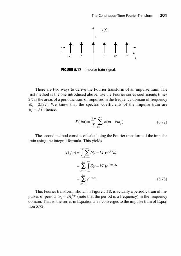
The Continuous-Time Fourier Transform 201
There are two ways to derive the Fourier transform of an impulse train. Thefirst method is the one introduced above: use the Fourier series coefficients times2 as the areas of a periodic train of impulses in the frequency domain of frequency
. We know that the spectral coefficients of the impulse train are; hence,
(5.72)
The second method consists of calculating the Fourier transform of the impulsetrain using the integral formula. This yields
(5.73)
This Fourier transform, shown in Figure 5.18, is actually a periodic train of im-pulses of period (note that the period is a frequency) in the frequencydomain. That is, the series in Equation 5.73 converges to the impulse train of Equa-tion 5.72.
02= T
X j t kT e dt
t kT e
k
j t
j
( ) ( )
( )
=
=
=
++
t
k
j kT
k
dt
e
+
=
+
=
+
= .
X jT
kk
( ) ( ).==
+20
a Tk = 10
2= T
FIGURE 5.17 Impulse train signal.

202 Fundamentals of Signals and Systems
((Lecture 19: Filtering))
FILTERING
In this section, we discuss an important application of the Fourier transform: fil-tering. Filtering is a rich topic often taught in graduate courses in electrical andcomputer engineering. We only give a rudimentary introduction to filtering toshow how the frequency-domain viewpoint can help us understand the concept ofshaping the spectrum of a signal by using filters. Sampling and modulation are alsoimportant applications of the Fourier transform. They will be studied in Chapters15 and 16, respectively.
Frequency-Selective Filters
Ideal frequency-selective filters are filters that let frequency components over agiven frequency band (the passband) pass through undistorted, while componentsat other frequencies (the stopband) are completely cut off. A typical scenarioshown in Figure 5.19, where filtering is needed, is when a noise n(t) is added to asignal x(t), but the noise has most, or all, of its energy at frequencies outside of thebandwidth of the signal. By linearity of the Fourier transform, the spectra of thesignal and the noise are also summed together. We want to recover the original sig-nal from its noisy measurement x1(t).
Here the noise spectrum is assumed to have all of its energy at higher frequen-cies than the bandwidth W of the signal. Thus, an ideal lowpass filter would per-fectly recover the signal, that is, , as seen in Figure 5.20. x t x t( ) ( )=
FIGURE 5.18 Fourier transform of an impulsetrain signal.
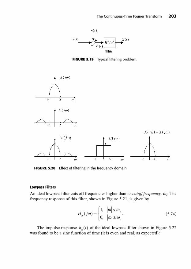
Lowpass Filters
An ideal lowpass filter cuts off frequencies higher than its cutoff frequency, c. Thefrequency response of this filter, shown in Figure 5.21, is given by
(5.74)
The impulse response of the ideal lowpass filter shown in Figure 5.22was found to be a sinc function of time (it is even and real, as expected):
h tlp
( )
H jlp
c
c
( ) :,
,.=
<1
0
The Continuous-Time Fourier Transform 203
FIGURE 5.19 Typical filtering problem.
FIGURE 5.20 Effect of filtering in the frequency domain.
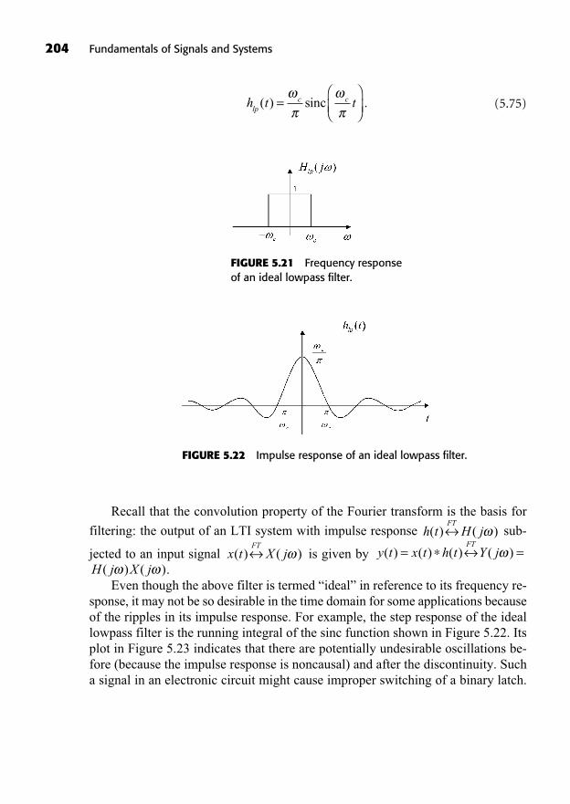
204 Fundamentals of Signals and Systems
(5.75)h t tlp
c c( ) .= sinc
FIGURE 5.21 Frequency responseof an ideal lowpass filter.
FIGURE 5.22 Impulse response of an ideal lowpass filter.
Recall that the convolution property of the Fourier transform is the basis for
filtering: the output of an LTI system with impulse response sub-
jected to an input signal is given by .
Even though the above filter is termed “ideal” in reference to its frequency re-sponse, it may not be so desirable in the time domain for some applications becauseof the ripples in its impulse response. For example, the step response of the ideallowpass filter is the running integral of the sinc function shown in Figure 5.22. Itsplot in Figure 5.23 indicates that there are potentially undesirable oscillations be-fore (because the impulse response is noncausal) and after the discontinuity. Sucha signal in an electronic circuit might cause improper switching of a binary latch.
H j X j( ) ( )y t x t h t Y j
FT( ) ( ) ( ) ( )= =x t X j
FT( ) ( )
h t H jFT
( ) ( )
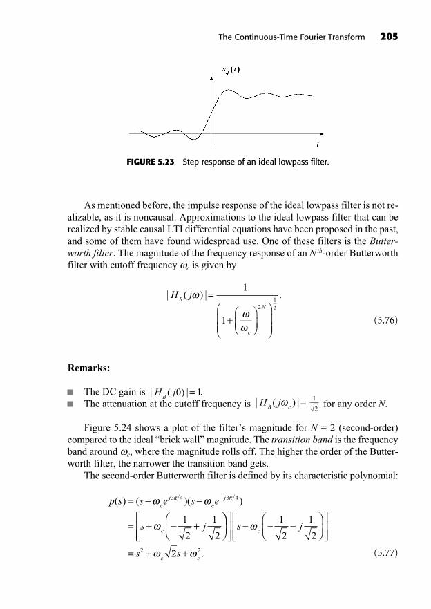
As mentioned before, the impulse response of the ideal lowpass filter is not re-alizable, as it is noncausal. Approximations to the ideal lowpass filter that can berealized by stable causal LTI differential equations have been proposed in the past,and some of them have found widespread use. One of these filters is the Butter-worth filter. The magnitude of the frequency response of an Nth-order Butterworthfilter with cutoff frequency c is given by
(5.76)
Remarks:
The DC gain is .The attenuation at the cutoff frequency is for any order N.
Figure 5.24 shows a plot of the filter’s magnitude for N = 2 (second-order)compared to the ideal “brick wall” magnitude. The transition band is the frequencyband around c, where the magnitude rolls off. The higher the order of the Butter-worth filter, the narrower the transition band gets.
The second-order Butterworth filter is defined by its characteristic polynomial:
(5.77)
p s s e s e
s j
cj
cj
c
( ) ( )( )=
= +
3 4 3 4
1
2
1
2
= +
s j
s
c
c
1
2
1
22 22 2s
c+ .
1
2| ( ) |H j
B c=
| ( ) |H jB
0 1=
| ( ) | .H jB
c
N
=
+
1
1
212
The Continuous-Time Fourier Transform 205
FIGURE 5.23 Step response of an ideal lowpass filter.
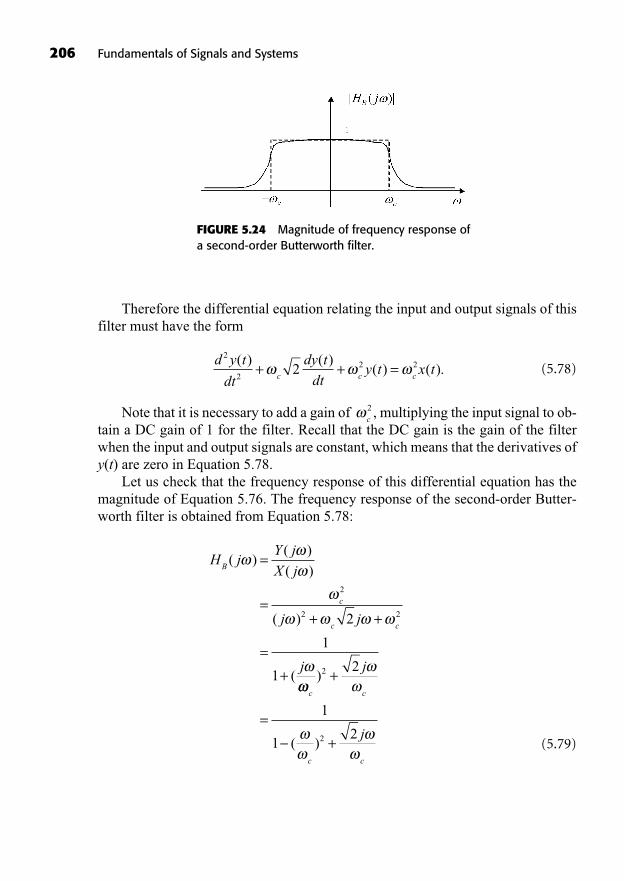
206 Fundamentals of Signals and Systems
Therefore the differential equation relating the input and output signals of thisfilter must have the form
(5.78)
Note that it is necessary to add a gain of , multiplying the input signal to ob-tain a DC gain of 1 for the filter. Recall that the DC gain is the gain of the filterwhen the input and output signals are constant, which means that the derivatives ofy(t) are zero in Equation 5.78.
Let us check that the frequency response of this differential equation has themagnitude of Equation 5.76. The frequency response of the second-order Butter-worth filter is obtained from Equation 5.78:
(5.79)
H jY j
X j
j j
j
B
c
c c
( )( )
( )
( )
(
=
=+ +
=+
2
2 22
1
1c c
c c
j
j
)
( )
2
2
2
1
12
+
=+
c2
d y t
dt
dy t
dty t x t
c c c
2
2
2 22( ) ( )
( ) ( ).+ + =
FIGURE 5.24 Magnitude of frequency response ofa second-order Butterworth filter.
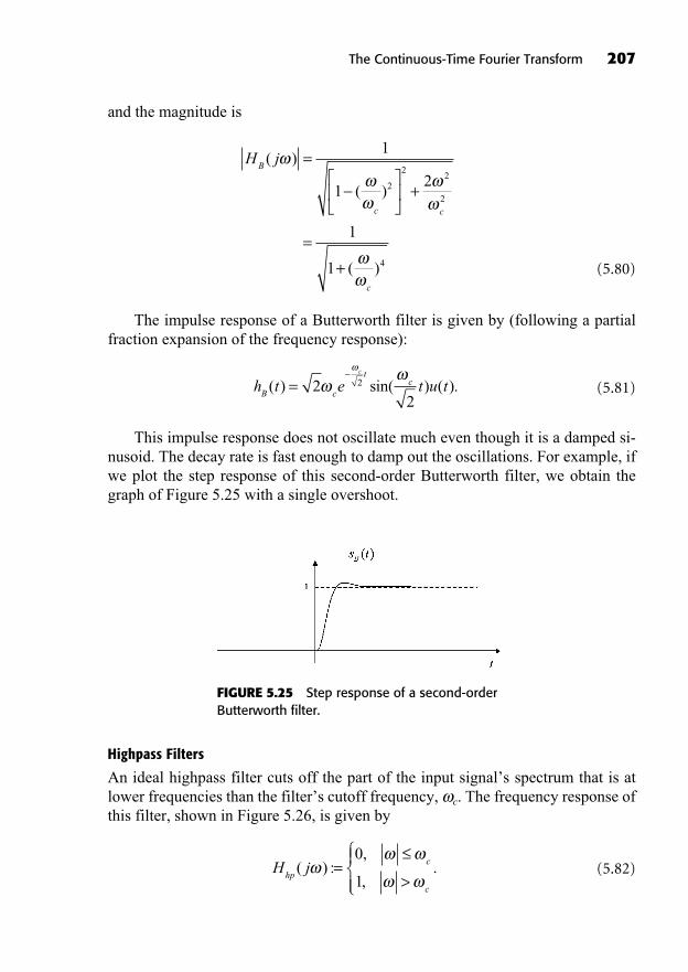
and the magnitude is
(5.80)
The impulse response of a Butterworth filter is given by (following a partialfraction expansion of the frequency response):
(5.81)
This impulse response does not oscillate much even though it is a damped si-nusoid. The decay rate is fast enough to damp out the oscillations. For example, ifwe plot the step response of this second-order Butterworth filter, we obtain thegraph of Figure 5.25 with a single overshoot.
h t e t u tB c
tc
c
( ) sin( ) ( ).= 22
2
H jB
c c
c
( )
( )
( )
=
+
=+
1
12
1
1
2
22
2
4
The Continuous-Time Fourier Transform 207
FIGURE 5.25 Step response of a second-orderButterworth filter.
Highpass Filters
An ideal highpass filter cuts off the part of the input signal’s spectrum that is atlower frequencies than the filter’s cutoff frequency, c. The frequency response ofthis filter, shown in Figure 5.26, is given by
(5.82)H jhp
c
c
( ) :,
,.=
>
0
1
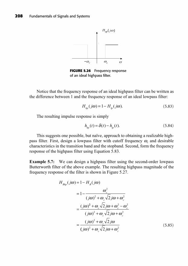
208 Fundamentals of Signals and Systems
Notice that the frequency response of an ideal highpass filter can be written asthe difference between 1 and the frequency response of an ideal lowpass filter:
(5.83)
The resulting impulse response is simply
(5.84)
This suggests one possible, but naïve, approach to obtaining a realizable high-pass filter. First, design a lowpass filter with cutoff frequency c and desirablecharacteristics in the transition band and the stopband. Second, form the frequencyresponse of the highpass filter using Equation 5.83.
Example 5.7: We can design a highpass filter using the second-order lowpassButterworth filter of the above example. The resulting highpass magnitude of thefrequency response of the filter is shown in Figure 5.27.
(5.85)
H j H j
j j
j
Bhp B
c
c c
( ) ( )
( )
( )
=
=+ +
=
1
12
2
2 2
22 2 2
2 2
2
2
2
2
+ +
+ +
=+
c c c
c c
c
j
j j
j j
( )
( )
(( )j jc c
2 22+ +
h t t h thp lp
( ) ( ) ( ).=
H j H jhp lp
( ) ( ).= 1
FIGURE 5.26 Frequency responseof an ideal highpass filter.
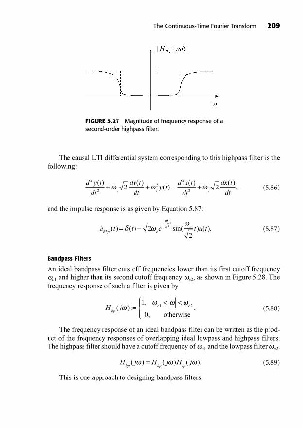
The causal LTI differential system corresponding to this highpass filter is thefollowing:
(5.86)
and the impulse response is as given by Equation 5.87:
(5.87)
Bandpass Filters
An ideal bandpass filter cuts off frequencies lower than its first cutoff frequencyc1 and higher than its second cutoff frequency c2, as shown in Figure 5.28. The
frequency response of such a filter is given by
(5.88)
The frequency response of an ideal bandpass filter can be written as the prod-uct of the frequency responses of overlapping ideal lowpass and highpass filters.The highpass filter should have a cutoff frequency of c1 and the lowpass filter c2.
(5.89)
This is one approach to designing bandpass filters.
H j H j H jbp hp lp
( ) ( ) ( ).=
H jbp
c c( ) :,
,.=
< <1
01 2
otherwise
h t t e t u tBhp c
tc
c
( ) ( ) sin( ) ( ).= 22
2
d y t
dt
dy t
dty t
d x t
dt
dc c c
2
2
22
22 2
( ) ( )( )
( )+ + = +
xx t
dt
( ),
The Continuous-Time Fourier Transform 209
FIGURE 5.27 Magnitude of frequency response of asecond-order highpass filter.
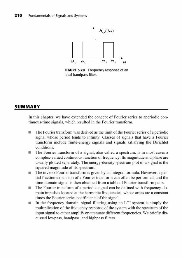
210 Fundamentals of Signals and Systems
SUMMARY
In this chapter, we have extended the concept of Fourier series to aperiodic con-tinuous-time signals, which resulted in the Fourier transform.
The Fourier transform was derived as the limit of the Fourier series of a periodicsignal whose period tends to infinity. Classes of signals that have a Fouriertransform include finite-energy signals and signals satisfying the Dirichlet conditions.The Fourier transform of a signal, also called a spectrum, is in most cases acomplex-valued continuous function of frequency. Its magnitude and phase areusually plotted separately. The energy-density spectrum plot of a signal is thesquared magnitude of its spectrum.The inverse Fourier transform is given by an integral formula. However, a par-tial fraction expansion of a Fourier transform can often be performed, and thetime-domain signal is then obtained from a table of Fourier transform pairs.The Fourier transform of a periodic signal can be defined with frequency-do-main impulses located at the harmonic frequencies, whose areas are a constanttimes the Fourier series coefficients of the signal.In the frequency domain, signal filtering using an LTI system is simply themultiplication of the frequency response of the system with the spectrum of theinput signal to either amplify or attenuate different frequencies. We briefly dis-cussed lowpass, bandpass, and highpass filters.
FIGURE 5.28 Frequency response of anideal bandpass filter.
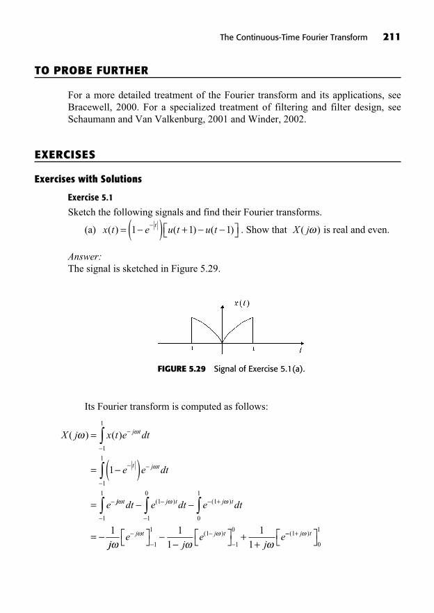
TO PROBE FURTHER
For a more detailed treatment of the Fourier transform and its applications, seeBracewell, 2000. For a specialized treatment of filtering and filter design, seeSchaumann and Van Valkenburg, 2001 and Winder, 2002.
EXERCISES
Exercises with Solutions
Exercise 5.1
Sketch the following signals and find their Fourier transforms.
(a) . Show that is real and even.
Answer:The signal is sketched in Figure 5.29.
X j( )x t e u t u tt
( ) ( ) ( )= ( ) +1 1 1
The Continuous-Time Fourier Transform 211
FIGURE 5.29 Signal of Exercise 5.1(a).
Its Fourier transform is computed as follows:
X j x t e dt
e e dt
e
j t
t j t
( ) ( )=
= ( )=
1
1
1
1
1
jj t j t j tdt e dt e dt+
=
1
11
1
01
0
1
1
( ) ( )
jje
je
jej t j t +
+1
11
1
011
11
( ) +( )1
0
1j t
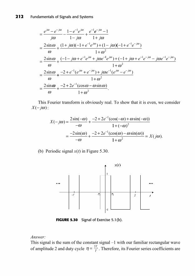
212 Fundamentals of Signals and Systems
This Fourier transform is obviously real. To show that it is even, we consider:
(b) Periodic signal x(t) in Figure 5.30.
X je
( )sin( ) (cos( ) sin( ))= + + +2 2 2 1
11
2 2 2
2
1
+
= + +
( )
sin( ) (cos( ) sin( ))e
11 2+= X j( ).
X j( )
= +1 11
1
j j je ej
e ej
e eej
j e e j
j
j
+
= + + + +
11
2 1 1 11sin ( )( ) ( )(( )
sin (
++
= + + +
1
1
2 1
1
2
1
e e
j e e j e
j
j 11 1 1
2
1
1
2
e j e e j e ej j j) ( )
sin
+ + ++
= ++ + + ++
=
2
1
2
1 1
2
e e e j e e ej j j j( ) ( )
sin + ++
2 2
1
1
2
e (cos sin ).
FIGURE 5.30 Signal of Exercise 5.1(b).
Answer:This signal is the sum of the constant signal –1 with our familiar rectangular waveof amplitude 2 and duty cycle . Therefore, its Fourier series coefficients are
2 1T
T=
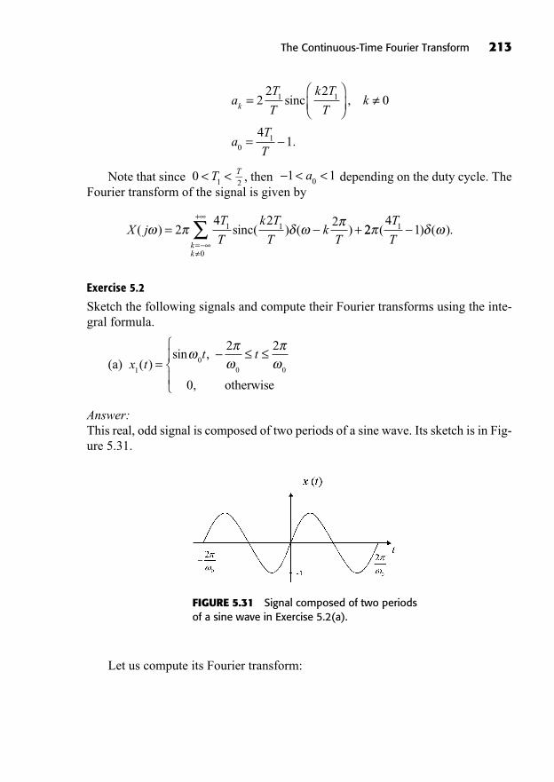
Note that since , then depending on the duty cycle. TheFourier transform of the signal is given by
Exercise 5.2
Sketch the following signals and compute their Fourier transforms using the inte-gral formula.
(a)
Answer:This real, odd signal is composed of two periods of a sine wave. Its sketch is in Fig-ure 5.31.
x tt t
10
0 0
2 2
0
( )sin ,
,
=otherwise
X jT
T
k T
Tk
Tkk
( ) ( ) ( )= +=
+
24 2 21 1
0
sinc 224
11( ) ( ).T
T
< <1 10a2T0 1< <T
aT
T
k T
Tk
aT
T
k =
=
22 2
0
41
1 1
01
sinc ,
.
The Continuous-Time Fourier Transform 213
FIGURE 5.31 Signal composed of two periodsof a sine wave in Exercise 5.2(a).
Let us compute its Fourier transform:
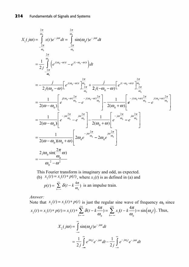
This Fourier transform is imaginary and odd, as expected.(b) , where x1(t) is as defined in (a) and
is an impulse train.
Answer:Note that is just the regular sine wave of frequency 0 since
. Thus,
X j t e dt
je e dt
j t
j t j t
2 0
12
0
( ) sin( )=
= 12
0
je e dtj t j t
x t x t p t x t t k xk
2 1 10
1
4( ) ( ) ( ) ( ) ( )= = =
=
+
(( ) sint k tk
= ( )=
+ 4
00
x t x t p t2 1( ) ( ) ( )=
)k4
0
t k(k=
+
p t( ) =
x t x t p t2 1( ) ( ) ( )=
X j x t e dt t e dj t j t1
2
2
0
0
0
( ) ( ) sin( )= = tt
je e dtj t j t= ( )
2
2
2
0
0
0 01
2( ) ( )
0
0
0
0
0
2
02
2
2= +j
je
jj t
( )( )
22
12
02
2
0
0
0
0
je
e
j t
( )
( )
( )
=jj j
e( ) ( )
( )
00
00
2 2
0
12 +
ee ej j+ +
=
( ) ( )
(
00
00
2 2
0
12 )) ( )
e e ej j j
+
2 2
0
2
0 0 01
2
=+
e
e
j
j
2
0 00
2
0
01
22
( )( )
=
2
22
0
2
00
02 2
0e
j
j
sin( )
214 Fundamentals of Signals and Systems
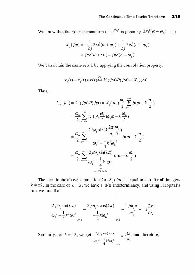
We know that the Fourier transform of is given by , so
We can obtain the same result by applying the convolution property:
Thus,
The term in the above summation for is equal to zero for all integers. In the case of , we have a indeterminacy, and using l’Hopital’s
rule we find that
Similarly, for , we get , and therefore,2
14
20
02 2
02
2
0
j k
kj
k
sin( )=
=
k = 2
2
14
2
12
0
02 2
02
2
0j k
k
j k
kk
sin( ) cos( )=
=00
2
2
0
02
0
2 2
k
jj
=
= =
0 0k = 2k ±2X j
2( )
X j X j P j X j kk
2 1 10 0
2 2( ) ( ) ( ) ( ) ( )= =
=
+
=
=
=
+0
10 0
00
2 2 2
2
2
X jk k
j
k
( ) ( )
sin(kk
kk
j
k
22
14
2
2
2
0
0
02 2
02
0
0
)
( )
=
=
+
0
02 2
02
0
14
sin( )(
k
k
= ± for k 2� ��� ���
kkk
0
2)
=
+
x t x t p t X j P j X jFT
2 1 1 2( ) ( ) ( ) ( ) ( ) ( ).= =
X jj j
j
2 0 0
0
1
22
1
22( ) ( ) ( )
( )
= + +
= + j ( )0
2 0( )e j t0
The Continuous-Time Fourier Transform 215
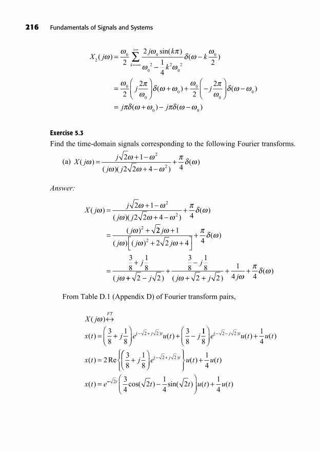
Exercise 5.3
Find the time-domain signals corresponding to the following Fourier transforms.
(a)
Answer:
From Table D.1 (Appendix D) of Fourier transform pairs,
X j
x t j e u t j
FT
j t
( )
( ) ( )( )= + ++38
18
38
2 2 118
14
238
18
2 2 +
= +
e u t u t
x t j
j t( ) ( ) ( )
( ) Re +
=
+e u t u t
x t e
j t( ) ( ) ( )
( )
2 2 14
+2 34
214
214
t t t u t u tcos( ) sin( ) ( ) ( )
X jj
j j
j
( )( )( )
( )
( )
= ++
+
= +
2 1
2 2 4 4
2
2
2 22 1
2 2 4 4
38
18
2
j
j j j
j
j
+
+ ++
=+
( ) ( )( )
( +++
+ ++ +
2 2
38
18
2 2
14 4j
j
j j j) ( )( )
X jj
j j( )
( )( )( )= +
++2 1
2 2 4 4
2
2
X jj k
kk
k2
0 0
02 2
02
0
2
2
14
2( )
sin( )( )=
=
+
= + +0
00
0
02
2
2
2j j( )
= +
( )
( ) ( )
0
0 0j j
216 Fundamentals of Signals and Systems
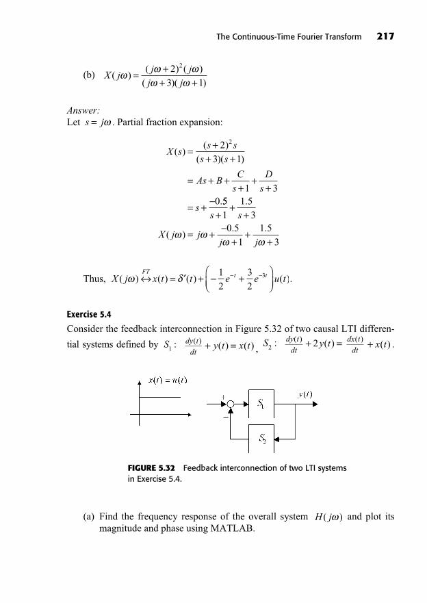
The Continuous-Time Fourier Transform 217
(b)
Answer:Let . Partial fraction expansion:
Thus, .
Exercise 5.4
Consider the feedback interconnection in Figure 5.32 of two causal LTI differen-
tial systems defined by , .x t( )+dx tdt( )y t2 ( )+ =dy t
dt( )S2 :y t x t( ) ( )+ =dy t
dt( )S1 :
X j x t t e e u tFT
t t( ) ( ) ( ) ( )= + +12
32
3
X ss s
s s
As BC
sD
s
s
( )( )
( )( )
.
= ++ +
= + ++
++
= +
23 1
1 30
2
551
1 53
0 51
1 53
s s
X j jj j
++
+
= ++
++
.
( ). .
s j=
X jj j
j j( )
( ) ( )( )( )
= ++ +
23 1
2
FIGURE 5.32 Feedback interconnection of two LTI systemsin Exercise 5.4.
(a) Find the frequency response of the overall system and plot itsmagnitude and phase using MATLAB.
H j( )
Answer:
The overall closed-loop frequency response is obtained by first writing theloop equations for the error signal e(t) (output of the summing junction) and theoutput.
Solving the first equation for , we obtain
Thus,
Magnitude and phase:
H jH j
H j H jj
jj
( )( )
( ) ( )=
+= +
++
+1
2 11
11
11
11
jj
j
j
jj j
+
= +
++
= ++ +
2
11
11
2
23 1( )( )
.
E jH j H j
X j
Y jH j
H
( )( ) ( )
( )
( )( )
(
=+
=+
11
1
2 1
1
2 jj H jX j
H j
) ( )( ).
( )
1� ���� ����
E j( )
E j X j H j H j E j
Y j H j E
( ) ( ) ( ) ( ) ( )
( ) ( ) (
= +
=2 1
1 jj )
S j Y j Y j X j
H jY jX j
1
1
: ( ) ( ) ( ) ( )
( )( )( )
+ =
= = 111
22
j
S j Y j Y j j X j X j
H
++ = +: ( ) ( ) ( ) ( ) ( ) ( )
22
12
( )( )( )
jY jX j
jj
= = ++
218 Fundamentals of Signals and Systems
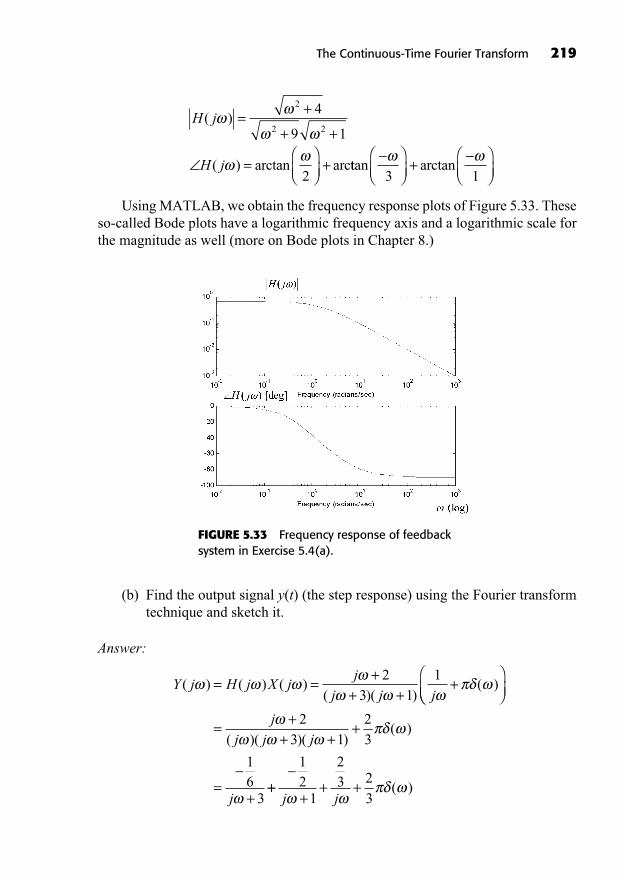
Using MATLAB, we obtain the frequency response plots of Figure 5.33. Theseso-called Bode plots have a logarithmic frequency axis and a logarithmic scale forthe magnitude as well (more on Bode plots in Chapter 8.)
H j
H j
( )
( ) arctan arc
= +
+ +
= +
2
2 2
4
9 1
2ttan arctan+
3 1
The Continuous-Time Fourier Transform 219
FIGURE 5.33 Frequency response of feedbacksystem in Exercise 5.4(a).
(b) Find the output signal y(t) (the step response) using the Fourier transformtechnique and sketch it.
Answer:
Y j H j X jj
j j j( ) ( ) ( )
( )( )( )= = +
+ ++2
3 11
= ++ +
+
=+
jj j j
j
23 1
23
16
3
( )( )( )( )
+++
+ +
12
1
23 2
3j j( )
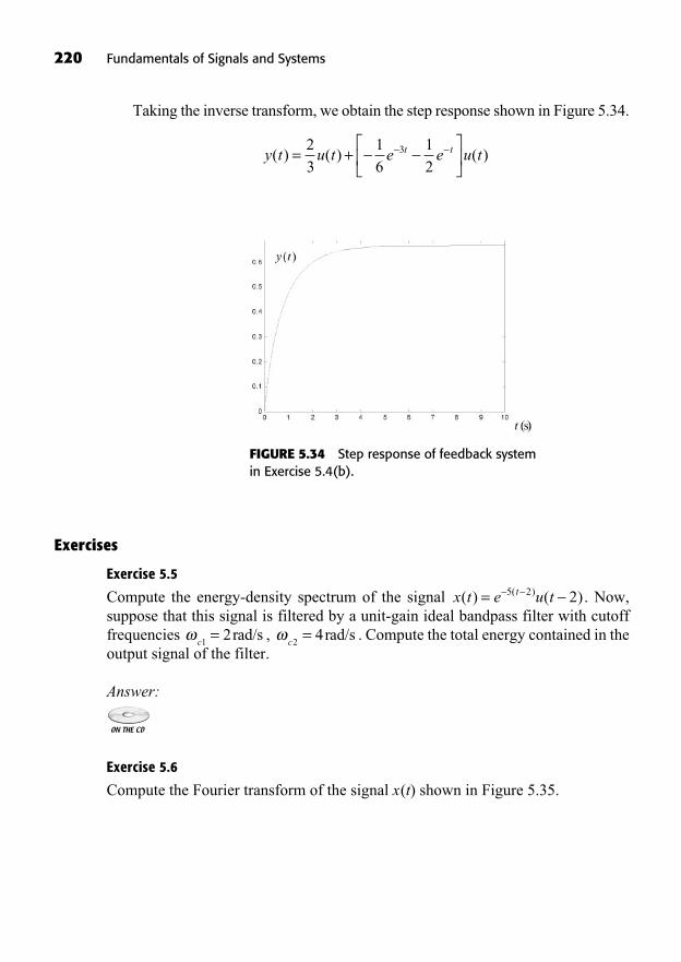
Taking the inverse transform, we obtain the step response shown in Figure 5.34.
y t u t e e u tt t( ) ( ) ( )= +23
16
12
3
220 Fundamentals of Signals and Systems
FIGURE 5.34 Step response of feedback systemin Exercise 5.4(b).
Exercises
Exercise 5.5
Compute the energy-density spectrum of the signal . Now,suppose that this signal is filtered by a unit-gain ideal bandpass filter with cutofffrequencies , . Compute the total energy contained in theoutput signal of the filter.
Answer:
Exercise 5.6
Compute the Fourier transform of the signal x(t) shown in Figure 5.35.
c24= rad/s
c12= rad/s
x t e u tt( ) ( )( )= 5 2 2
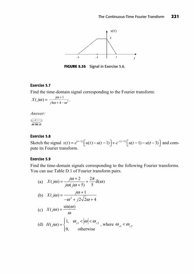
Exercise 5.7
Find the time-domain signal corresponding to the Fourier transform:
.
Answer:
Exercise 5.8
Sketch the signal and com-pute its Fourier transform.
Exercise 5.9
Find the time-domain signals corresponding to the following Fourier transforms.You can use Table D.1 of Fourier transform pairs.
(a)
(b)
(c)
(d) , where c c1 2<H j c c( ),
,=
< <1
01 2
otherwise
X j( )sin( )=
X jj
j( ) = +
+ +1
2 2 42
X jj
j j( )
( )( )= +
++2
525
x t e u t u t e u t ut t( ) ( ) ( ) ( ) (( ) ( )= +1 11 1 tt 3)
j
j
++
1
4 4 2X j( ) =
The Continuous-Time Fourier Transform 221
FIGURE 5.35 Signal in Exercise 5.6.
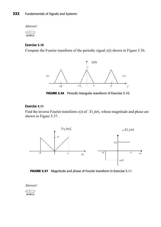
222 Fundamentals of Signals and Systems
Answer:
Exercise 5.10
Compute the Fourier transform of the periodic signal x(t) shown in Figure 5.36.
FIGURE 5.36 Periodic triangular waveform of Exercise 5.10.
Exercise 5.11
Find the inverse Fourier transform x(t) of , whose magnitude and phase areshown in Figure 5.37.
X j( )
FIGURE 5.37 Magnitude and phase of Fourier transform in Exercise 5.11.
Answer:
223
The Laplace Transform6
In This Chapter
Definition of the Two-Sided Laplace TransformInverse Laplace TransformConvergence of the Two-Sided Laplace TransformPoles and Zeros of Rational Laplace TransformsProperties of the Two-Sided Laplace TransformAnalysis and Characterization of LTI Systems using the Laplace TransformDefinition of the Unilateral Laplace TransformProperties of the Unilateral Laplace TransformSummaryTo Probe FurtherExercises
((Lecture 20: Definition of the Laplace Transform))
So far, we have studied the Fourier series and the Fourier transform for theanalysis of periodic and aperiodic signals, and linear time-invariant (LTI)systems. These tools are useful because they allow us to analyze continuous-
time signals and systems in the frequency domain. In particular, signals can berepresented as linear combinations of periodic complex exponentials, which areeigenfunctions of LTI systems, but if we replace j with the more general complexvariable s in the Fourier transform equations, we obtain the Laplace transform, ageneralization of the Fourier transform.

224 Fundamentals of Signals and Systems
The Fourier transform was defined only for signals that taper off at infinity,that is, signals of finite energy or signals that are absolutely integrable. On the otherhand, the Laplace transform of an unbounded signal or of an unstable impulse re-sponse can be defined. The Laplace transform can also be used to analyze differ-ential LTI systems with nonzero initial conditions.
DEFINITION OF THE TWO-SIDED LAPLACE TRANSFORM
The two-sided Laplace transform of x(t) is defined as follows:
(6.1)
where s is a complex variable. Notice that the Fourier transform is given by thesame equation, but with .
Let the complex variable be written as . Then the Laplace transformcan be interpreted as the Fourier transform of the signal :
(6.2)
Given x(t), this integral may or may not converge, depending on the value of(the real part of s).
Example 6.1: Let us find the Laplace transform of the signalshown in Figure 6.1.x t e u t aat( ) ( ),= R
X j x t e e dtt j t( ) ( ) .+ =+
x t e t( )s j= +
s j=
X s x t e dtst( ) : ( ) ,=+
FIGURE 6.1 Real decayingexponential signal.
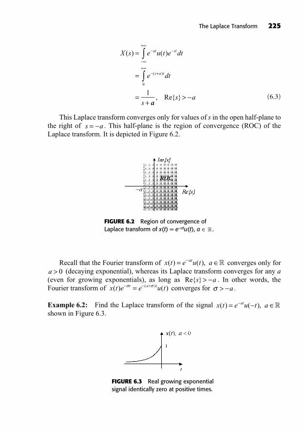
(6.3)
This Laplace transform converges only for values of s in the open half-plane tothe right of . This half-plane is the region of convergence (ROC) of theLaplace transform. It is depicted in Figure 6.2.
s a=
X s e u t e dt
e dt
s
at st
s a t
( ) ( )
( )
=
=
=+
+
++
0
1
aas a, Re{ }>
The Laplace Transform 225
FIGURE 6.2 Region of convergence of Laplace transform of x(t) = e–atu(t), a .�
Recall that the Fourier transform of converges only for(decaying exponential), whereas its Laplace transform converges for any a
(even for growing exponentials), as long as . In other words, theFourier transform of converges for .
Example 6.2: Find the Laplace transform of the signal shown in Figure 6.3.
x t e u t aat( ) ( ),= �
> ax t e e u tt a t( ) ( )( )+=Re{ }s a>
a > 0x t e u t aat( ) ( ),= R
FIGURE 6.3 Real growing exponentialsignal identically zero at positive times.
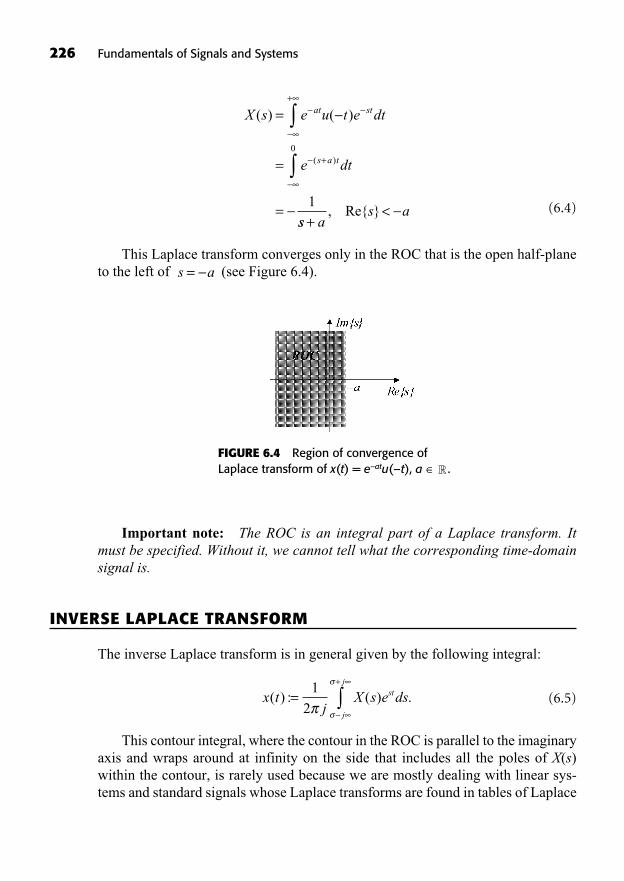
226 Fundamentals of Signals and Systems
(6.4)
This Laplace transform converges only in the ROC that is the open half-planeto the left of (see Figure 6.4).s a=
X s e u t e dt
e dt
at st
s a t
( ) ( )
( )
=
=
=
+
+0
1ss a
s a+
<, Re{ }
FIGURE 6.4 Region of convergence ofLaplace transform of x(t) = e–atu(–t), a .�
Important note: The ROC is an integral part of a Laplace transform. Itmust be specified. Without it, we cannot tell what the corresponding time-domainsignal is.
INVERSE LAPLACE TRANSFORM
The inverse Laplace transform is in general given by the following integral:
(6.5)
This contour integral, where the contour in the ROC is parallel to the imaginaryaxis and wraps around at infinity on the side that includes all the poles of X(s)within the contour, is rarely used because we are mostly dealing with linear sys-tems and standard signals whose Laplace transforms are found in tables of Laplace
x tj
X s e dsst
j
j
( ) : ( ) .=+1
2
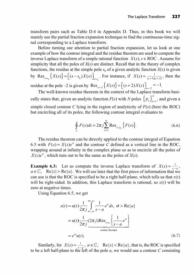
transform pairs such as Table D.4 in Appendix D. Thus, in this book we willmainly use the partial fraction expansion technique to find the continuous-time sig-nal corresponding to a Laplace transform.
Before turning our attention to partial fraction expansion, let us look at oneexample of how the contour integral and the residue theorem are used to compute theinverse Laplace transform of a simple rational function . Assume forsimplicity that all the poles of X(s) are distinct. Recall that in the theory of complexfunctions, the residue at the simple pole s0 of a given analytic function X(s) is given
by . For instance, if , then the
residue at the pole –2 is given by .The well-known residue theorem in the context of the Laplace transform basi-
cally states that, given an analytic function F(s) with N poles , and given a
simple closed contour C lying in the region of analyticity of F(s) (here the ROC)but encircling all of its poles, the following contour integral evaluates to
(6.6)
The residue theorem can be directly applied to the contour integral of Equation6.5 with and the contour C defined as a vertical line in the ROC,wrapping around at infinity in the complex plane so as to encircle all the poles of
, which turn out to be the same as the poles of X(s).
Example 6.3: Let us compute the inverse Laplace transform of ,. We will see later that the first piece of information that we
can use is that the ROC is specified to be a right half-plane, which tells us that x(t)will be right-sided. In addition, this Laplace transform is rational, so x(t) will bezero at negative times.
Using Equation 6.5, we get
(6.7)
Similarly, for , , that is, the ROC is specifiedto be a left half-plane to the left of the pole a, we would use a contour C consisting
a s a<C, Re{ } Re{ }s a
1X s( ) =
x t u tj s a
e ds a
u t
st
j
j
( ) ( ) , Re{ }
(
= >
=
+1
2
1
)) ( )1
22
1
jj
s ae
s astRes
residue theor
=
eem� ����� �����
= e u tat ( ).
a s a>C, Re{ } Re{ }s a
1X s( ) =
X s est( )
F s X s est( ) ( )=
F s ds j F sC
s pk
k( ) ( ) .� = { }=
=
21
ResN
pk k
N{ } =1
= 1Ress s
X s s X s= ={ } = +
2 22( ) ( ) ( )
s s( )( )+ +1
1 2X s( ) =Res
s s s sX s s s X s= =
{ } =0 0
0( ) ( ) ( )
X s s( ), ROC
The Laplace Transform 227
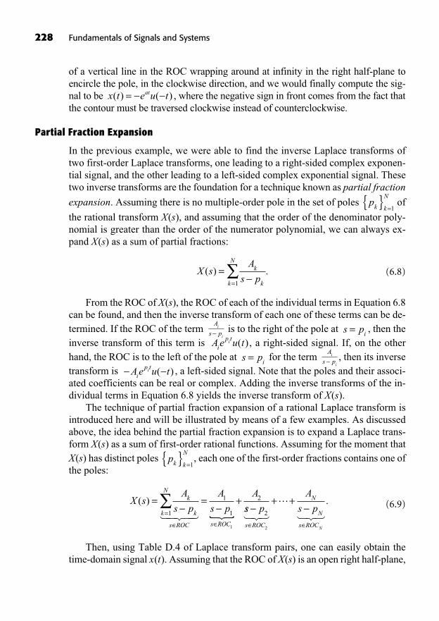
of a vertical line in the ROC wrapping around at infinity in the right half-plane toencircle the pole, in the clockwise direction, and we would finally compute the sig-nal to be , where the negative sign in front comes from the fact thatthe contour must be traversed clockwise instead of counterclockwise.
Partial Fraction Expansion
In the previous example, we were able to find the inverse Laplace transforms oftwo first-order Laplace transforms, one leading to a right-sided complex exponen-tial signal, and the other leading to a left-sided complex exponential signal. Thesetwo inverse transforms are the foundation for a technique known as partial fraction
expansion. Assuming there is no multiple-order pole in the set of poles of
the rational transform X(s), and assuming that the order of the denominator poly-nomial is greater than the order of the numerator polynomial, we can always ex-pand X(s) as a sum of partial fractions:
(6.8)
From the ROC of X(s), the ROC of each of the individual terms in Equation 6.8can be found, and then the inverse transform of each one of these terms can be de-termined. If the ROC of the term is to the right of the pole at , then theinverse transform of this term is , a right-sided signal. If, on the otherhand, the ROC is to the left of the pole at for the term , then its inversetransform is , a left-sided signal. Note that the poles and their associ-ated coefficients can be real or complex. Adding the inverse transforms of the in-dividual terms in Equation 6.8 yields the inverse transform of X(s).
The technique of partial fraction expansion of a rational Laplace transform isintroduced here and will be illustrated by means of a few examples. As discussedabove, the idea behind the partial fraction expansion is to expand a Laplace trans-form X(s) as a sum of first-order rational functions. Assuming for the moment thatX(s) has distinct poles , each one of the first-order fractions contains one ofthe poles:
(6.9)
Then, using Table D.4 of Laplace transform pairs, one can easily obtain thetime-domain signal x(t). Assuming that the ROC of X(s) is an open right half-plane,
X sA
s p
A
s p
Ak
kk
N
s ROC s ROC
( ) = = +=1
1
1
2
1
� �� �� �ss p
A
s p
s ROC
N
N
s ROCN
+ +2
2
������
.
pk k
N{ } =1
A e u tip ti ( )
A
s pi
is pi=
A e u tip ti ( )
s pi=A
s pi
i
X sA
s pk
kk
N
( ) .==1
pk k
N{ } =1
x t e u tat( ) ( )=
228 Fundamentals of Signals and Systems
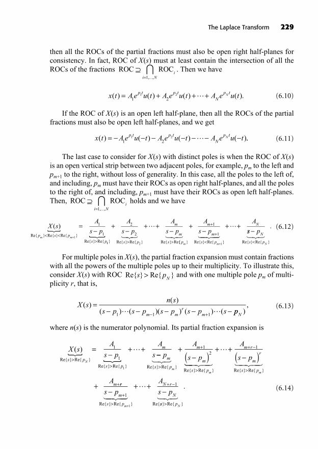
then all the ROCs of the partial fractions must also be open right half-planes forconsistency. In fact, ROC of X(s) must at least contain the intersection of all theROCs of the fractions . Then we have
(6.10)
If the ROC of X(s) is an open left half-plane, then all the ROCs of the partialfractions must also be open left half-planes, and we get
(6.11)
The last case to consider for X(s) with distinct poles is when the ROC of X(s)is an open vertical strip between two adjacent poles, for example, pm to the left andpm+1 to the right, without loss of generality. In this case, all the poles to the left of,and including, pm must have their ROCs as open right half-planes, and all the polesto the right of, and including, pm+1 must have their ROCs as open left half-planes.Then, holds and we have
(6.12)
For multiple poles in X(s), the partial fraction expansion must contain fractionswith all the powers of the multiple poles up to their multiplicity. To illustrate this,consider X(s) with ROC and with one multiple pole pm of multi-plicity r, that is,
(6.13)
where n(s) is the numerator polynomial. Its partial fraction expansion is
(6.14)
X sA
s p
A
ss p
s p
m
N
( )Re{ } Re{ }
Re{ } Re{ }>
>
= + +��
1
1
1
+( )
>
+
>
p
A
s pm
s p
m
m
s pmm
Re{ } Re{ }Re{ } Re{ }
���
12
�� �� ��
� �� ��
+ +( )
+
+
>
+
A
s p
A
m r
m
r
s p
m
m
1
Re{ } Re{ }
rr
m
s p
N r
Ns p
A
s p
m
+ ++
>
+
+
1
1
1Re{ } Re{ } Re{��� ��
ss pN} Re{ }
.
>���
X sn s
s p s p s p s p sm mr
m
( )( )
( ) ( )( ) ( ) (=
+1 1 1 ppN ),
Re{ } Re{ }s pN>
X sA
s pp s p
s pm m
( )Re{ } Re{ } Re{ }
Re{ } Re{< <
>+
=1
1
1�
11 2
2
2
} Re{ } Re{ } Re{ } Re
� ���+ + +
> >
A
s p
A
s p
s p
m
m
s {{ } Re{ } Re{ }p
m
m
s p
N
m m
A
s p
A
��� ��� ��+ + ++
+
< +
1
1
1
ss pN
s pN<Re{ } Re{ }
.���
ROC ROC=
ii N1, ,…∩
x t A e u t A e u t A e u tp t p tN
p tN( ) ( ) ( ) ( )= 1 21 2 ..
x t A e u t A e u t A e u tp t p tN
p tN( ) ( ) ( ) ( ).= + + +1 21 2
ROC ROC=
ii N1, ,…∩
The Laplace Transform 229
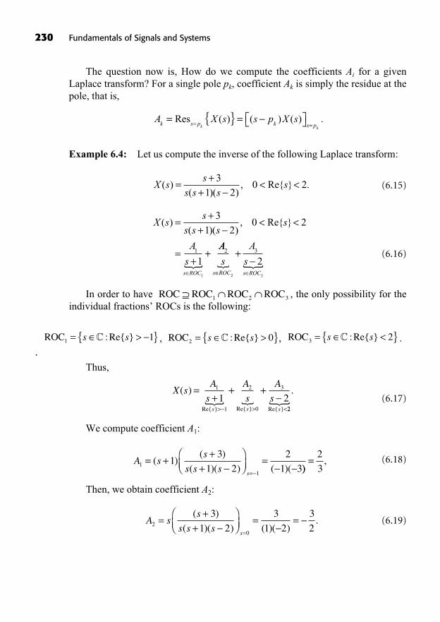
The question now is, How do we compute the coefficients Ai for a givenLaplace transform? For a single pole pk, coefficient Ak is simply the residue at thepole, that is,
Example 6.4: Let us compute the inverse of the following Laplace transform:
(6.15)
(6.16)
In order to have , the only possibility for theindividual fractions’ ROCs is the following:
.
, , .
Thus,
(6.17)
We compute coefficient A1:
(6.18)
Then, we obtain coefficient A2:
(6.19)A ss
s s ss
2
0
3
1 2
3
1 2
3
2=
++
= ==
( )
( )( ) ( )( ).
A ss
s s ss
1
1
13
1 2
2
1 3= +
++
==
( )( )
( )( ) ( )( )),=
2
3
X sA
s
A
s
A
ss s s
( )
Re{ } Re{ } Re{ }
=+
+ +
> > <
1
1
2
0
3
1 2� �22�
.
ROC3 2= <{ }s sC :Re{ }ROC2 0= >{ }s sC :Re{ }ROC1 1= >{ }s sC :Re{ }
ROC ROC ROC ROC1 2 3
X ss
s s ss
A
ss ROC
( )( )( )
, Re{ }=+
+< <
=+
+
3
1 20 2
11
1
�
AA
s
A
ss ROC s ROC
2 3
2 3
2+
� �
X ss
s s ss( )
( )( ), Re{ } .=
++
< <3
1 20 2
A X s s p X sk s p k s pk k
= { } == =Res ( ) ( ) ( ) .
230 Fundamentals of Signals and Systems
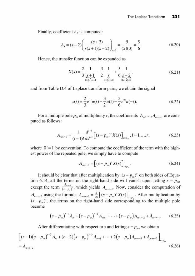
Finally, coefficient A3 is computed:
(6.20)
Hence, the transfer function can be expanded as
(6.21)
and from Table D.4 of Laplace transform pairs, we obtain the signal
(6.22)
For a multiple pole pm of multiplicity r, the coefficients are com-puted as follows:
(6.23)
where by convention. To compute the coefficient of the term with the high-est power of the repeated pole, we simply have to compute
(6.24)
It should be clear that after multiplication by on both sides of Equa-tion 6.14, all the terms on the right-hand side will vanish upon letting s = pm,
except the term , which yields . Now, consider the computation of
using the formula . After multiplication by, the terms on the right-hand side corresponding to the multiple pole
become
(6.25)
After differentiating with respect to s and letting s = pm, we obtain
(6.26)
( ) ( )r s p A r s p A s pm
r
m m
r
m m( ) + ( ) + ++1 2 22 3
1 (( ) +
=
+ +=
+
A A
A
m r m rs p
m r
m3 2
2
s p A s p A s p A Am
r
m m
r
m m m r m( ) + ( ) + + ( ) ++ +1 2
1 2 ++r 1.
( )s pmr
s p X smr
s pm=( ) ( )d
dsAm r+ =2Am r+ 2
Am r+ 1
A
s pm r
m
r+
( )1
( )s pmr
A s p X sm r mr
s pm+ =
=1 ( ) ( ) .
0 1!=
Ai
d
dss p X sm r i
i
i mr
s pm+ =
=1
1
1
1( )!( ) ( ) , ii r= 1, , ,…
A Am m r, ,… + 1
x t e u t u t e u tt t( ) ( ) ( ) ( ).=2
3
3
2
5
62
X ss s ss s
( )
Re{ } Re{ } Re{
=+
+
> >
2
3
1
1
3
2
1 5
6
1
21 0� �
ss}
,
<2�
A ss
s s ss
3
2
23
1 2
5
2 3
5=
++
= ==
( )( )
( )( ) ( )( ) 66.
The Laplace Transform 231
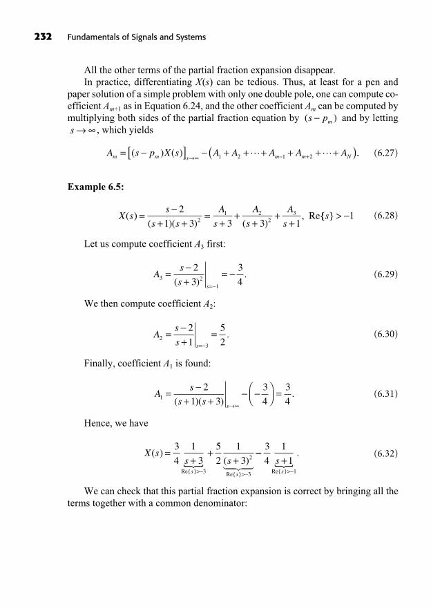
All the other terms of the partial fraction expansion disappear.In practice, differentiating X(s) can be tedious. Thus, at least for a pen and
paper solution of a simple problem with only one double pole, one can compute co-efficient Am+1 as in Equation 6.24, and the other coefficient Am can be computed bymultiplying both sides of the partial fraction equation by and by letting
, which yields
(6.27)
Example 6.5:
(6.28)
Let us compute coefficient A3 first:
(6.29)
We then compute coefficient A2:
(6.30)
Finally, coefficient A1 is found:
(6.31)
Hence, we have
(6.32)
We can check that this partial fraction expansion is correct by bringing all theterms together with a common denominator:
X ss ss s
( )( )
Re{ } Re{ }
=+
++
> >
3
4
1
3
5
2
1
33
2
3
� ��� �� +>
3
4
1
11
ssRe{ }
.�
As
s ss
1
2
1 3
3
4
3
4=
+ +=
( )( ).
As
s s2
3
2
1
5
2=
+=
=
.
As
ss
3 21
2
3
3
4=
+=
=( ).
X ss
s s
A
s
A
s
A
s( )
( )( ) ( ), Re=
+ +=
++
++
+2
1 3 3 3 121 2
23 {{ }s > 1
A s p X s A A A A Am m s m m N= [ ] + + + + + +( )+( ) ( ) 1 2 1 2 ..
s( )s pm
232 Fundamentals of Signals and Systems

(6.33)
Finally, using Table D.4 of Laplace transform pairs, we obtain
(6.34)
A pair of complex conjugate poles in a Laplace transform can be dealt with in-dividually using the residue technique outlined above. The two complex coeffi-cients obtained are complex conjugates of each other. A pair of complex conjugatepoles can also be treated by including a second-order term in the partial fraction ex-pansion. The idea is to make use of the damped or growing sinusoids in the tableof Laplace transforms, such as
(6.35)
(6.36)
by creating a term in the partial fraction expansion. It is perhaps best toexplain this technique by means of an example.
Example 6.6: Let us compute the inverse of the following Laplace transform:
(6.37)
Note that , so that the complex poles are
and . The transform X(s) can be expanded as follows:p j1 1 3=p j1 1 3= +s s s2 2 22 4 1 3+ + = + +( ) ( )
X ss s
s s ss( ) , Re{ } .=
++ +( ) >
2 3 2
2 40
2
2
A B s
s0
20
2
+ ++ +
( )
( )
e ts
sst L +
+ +>cos( )
( ), Re{ }0 2
02
e ts
st L
+ +>sin( )
( ), Re{ } ,0
02
02
x t e te e u tt t t( ) ( )= +3
4
5
2
3
43 3
X ss s s
s s
( )( )
( )( )
=+
++ +
=+ + +
3
4
1
3
5
2
1
3
3
4
1
1
3 1 3 10
2
(( ) ( )
( )( )s s
s s
s s s
+ ++ +
=+ + + +
1 3 3
4 1 3
3 12 9 10 10
2
2
2
+ +
=+ +
=
3 18 27
4 1 3
4 8
4 1 3
2
2
2
s s
s s
s
s s
s
( )( )
( )( ) + +2
1 3 2( )( ).
s s
The Laplace Transform 233
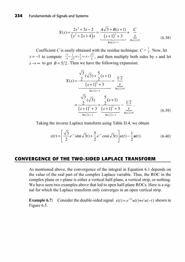
(6.38)
Coefficient C is easily obtained with the residue technique: C = . Now, let
to compute , and then multiply both sides by s and let
to get . Then we have the following expansion:
(6.39)
Taking the inverse Laplace transform using Table D.4, we obtain
(6.40)
CONVERGENCE OF THE TWO-SIDED LAPLACE TRANSFORM
As mentioned above, the convergence of the integral in Equation 6.1 depends onthe value of the real part of the complex Laplace variable. Thus, the ROC in thecomplex plane or s-plane is either a vertical half-plane, a vertical strip, or nothing.We have seen two examples above that led to open half-plane ROCs. Here is a sig-nal for which the Laplace transform only converges in an open vertical strip.
Example 6.7: Consider the double-sided signal shown inFigure 6.5.
x t e u t e u tt t( ) ( ) ( )= 2 +
x t e t e t u tt t( ) sin( ) cos( ) ( )= +3
23
5
23
1
2uu t( ).
X ss
ss
( )( ) ( )
Re{ }
=+ +
+( ) +>
32
352
1
1 32
1� ���� ����
=+( ) +
+
>
>
1 2
32
3
1 3
52
0
2
1
s
s
s
s
Re{ }
Re{ }
( )
�
� �� ��
(( ).
Re{ }Re{ }
s
s s
ss
+
+( ) +>
>
1
1 3
1 22
10� �� �� �
B = 5 2s
= + =3
3
1
3
1
2
3
2A As = 1
1
2
X ss s
s s s
A B s
s( )
( )
Re
=+
+ +( ) =+ ++( ) +
2 3 2
2 4
3 1
1 3
2
2 2
{{ }Re{ }
.
ss
C
s
>>
+
10� ��� ��� �
234 Fundamentals of Signals and Systems
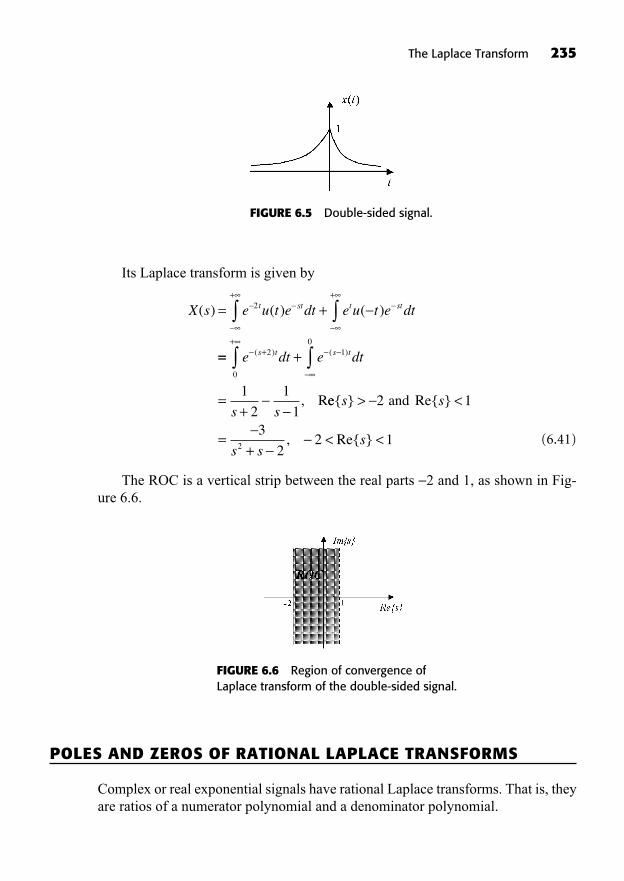
The Laplace Transform 235
Its Laplace transform is given by
(6.41)
The ROC is a vertical strip between the real parts 2 and 1, as shown in Fig-ure 6.6.
X s e u t e dt e u t e dtt st t st( ) ( ) ( )= ++ +
2
== +
=+
++
e dt e dt
s s
s t s t( ) ( )
, R
2
0
10
1
2
1
1ee{ } Re{ }
, Re{ }
s s
s ss
> <
=+
< <
2 1
3
22 12
and
FIGURE 6.5 Double-sided signal.
FIGURE 6.6 Region of convergence ofLaplace transform of the double-sided signal.
POLES AND ZEROS OF RATIONAL LAPLACE TRANSFORMS
Complex or real exponential signals have rational Laplace transforms. That is, theyare ratios of a numerator polynomial and a denominator polynomial.
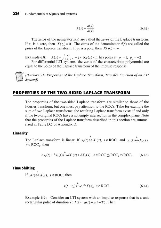
236 Fundamentals of Signals and Systems
(6.42)
The zeros of the numerator n(s) are called the zeros of the Laplace transform.If z1 is a zero, then . The zeros of the denominator d(s) are called thepoles of the Laplace transform. If p1 is a pole, then .
Example 6.8: , has poles at .For differential LTI systems, the zeros of the characteristic polynomial are
equal to the poles of the Laplace transform of the impulse response.
((Lecture 21: Properties of the Laplace Transform, Transfer Function of an LTISystem))
PROPERTIES OF THE TWO-SIDED LAPLACE TRANSFORM
The properties of the two-sided Laplace transform are similar to those of theFourier transform, but one must pay attention to the ROCs. Take for example thesum of two Laplace transforms: the resulting Laplace transform exists if and onlyif the two original ROCs have a nonempty intersection in the complex plane. Notethat the properties of the Laplace transform described in this section are summa-rized in Table D.5 of Appendix D.
Linearity
The Laplace transform is linear. If and , then
(6.43)
Time Shifting
If , then
(6.44)
Example 6.9: Consider an LTI system with an impulse response that is a unitrectangular pulse of duration T: . Thenh t u t u t T( ) ( ) ( )=
x t t e X s sL
st( ) ( ),00 ROC.
x t X s sL
( ) ( ), ROC
ax t bx t aX s bX s sL
1 2 1 2( ) ( ) ( ) ( ),+ + ROC ROC ROC1 22 .
s ROC2
x t X sL
2 2( ) ( ),x t X s sL
1 1( ) ( ), ROC1
p p1 21 2= =,sRe{ }< <2 1s
s s
++
2 1
22X s( ) =
X p( )1 =X z( )1 0=
X sn s
d s( )
( )
( )=
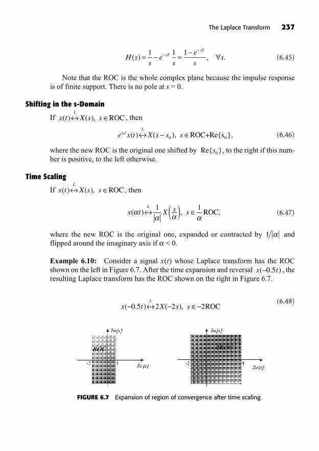
(6.45)
Note that the ROC is the whole complex plane because the impulse responseis of finite support. There is no pole at s = 0.
Shifting in the s-Domain
If , then
(6.46)
where the new ROC is the original one shifted by , to the right if this num-ber is positive, to the left otherwise.
Time Scaling
If , then
(6.47)
where the new ROC is the original one, expanded or contracted by andflipped around the imaginary axis if < 0.
Example 6.10: Consider a signal x(t) whose Laplace transform has the ROCshown on the left in Figure 6.7. After the time expansion and reversal , theresulting Laplace transform has the ROC shown on the right in Figure 6.7.
(6.48)x t X s s
L
( . ) ( ),0 5 2 2 2ROC
x t( . )0 5
1
x t X s sL
( ) ,( )1 1ROC,
x t X s sL
( ) ( ), ROC
Re{ }s0
e x t X s s ss tL
00( ) ( ), },ROC+Re{s0
x t X s sL
( ) ( ), ROC
H ss
es
e
sssT
sT
( ) , .= =1 1 1
The Laplace Transform 237
FIGURE 6.7 Expansion of region of convergence after time scaling.
Conjugation
If , then
(6.49)
Therefore, for x(t) real, .An important consequence is that if x(t) is real and X(s) has a pole (or zero) at
, then X(s) has also a pole (or zero) at the complex conjugate point .Thus, the complex poles and zeros of the Laplace transform of a real signal alwayscome in conjugate pairs.
Convolution Property
If and , then
(6.50)
This is of course an extremely useful property for LTI system analysis. Notethat the resulting ROC includes the intersection of the two original ROCs, but itmay be larger, for example, when a pole-zero cancellation occurs.
Example 6.11: The response of the LTI system with to the input is given by the inverse Laplace transform of Y(s):
(6.51)
and
(6.52)
Expanding this transform into partial fractions, we get
(6.53)Y ss
s
A
s
B
ss( )
( )
( ) ( ) ( ), Re{ } .=
++
=+
++
>2 3
2 2 22
2 2
Y s H s X ss
s s
s
ss( ) ( ) ( )
( )
( )( )
( )
( ), {= =
++ +
++
2 3
2 1
1
2::Re{ } } { :Re{ } } { :Re{ } }
(
s s s s s
s
> > = >
=+
2 1 1
2 3))
( ), Re{ }
ss
+>
222 (after the pole-zero cancelllation).
h t H ss
s ss
x t X s
L
L
( ) ( )( )( )
, Re{ }
( ) (
=+
+ +>
2 3
2 11
)) , Re{ }=+
+ =++
>1
21
1
22
s
s
ss
x t e u t tt( ) ( ) ( )= +2
h t e e u tt t( ) ( )= +2
x t x t X s X s sL
1 2 1 2( ) ( ) ( ) ( ), .ROC ROC ROC1 2
x t X s sL
2 2( ) ( ), ROC2x t X s sL
1 1( ) ( ), ROC1
s s=0
s s=0
X s X s( ) ( )=
x t X s sL
( ) ( ), ROC.
x t X s sL
( ) ( ), ROC
238 Fundamentals of Signals and Systems
We find coefficient B first:
(6.54)
and coefficient A is then obtained:
(6.55)
Therefore, using Table D.4 of Laplace transform pairs, we obtain
(6.56)
Differentiation in the Time Domain
If , then
(6.57)
ROC1 can be larger than ROC, namely when there is a pole-zero cancellationat s = 0.
Differentiation in the Frequency Domain
If , then
(6.58)
This property is useful to obtain the Laplace transform of signals of the form.
Integration in the Time Domain
If , then:
(6.59)x dsX s s s s
t L( ) ( ), :Re .{ }1
ROC ROC { }>01
x t X s sL
( ) ( ), ROC
x t te u tat( ) ( )=
tx tdX s
dss
L( )
( ), ROC.
x t X s sL
( ) ( ), ROC
dx t
dtsX s s
L( )( ), ROC ROC,1
x t X s sL
( ) ( ), ROC
y t e te u tt t( ) ( ).= 2 2 2
2 3
22
s
sA
s
++
= ==+
.
( ),
2 3
11
2
sB
s
+= =
=
The Laplace Transform 239
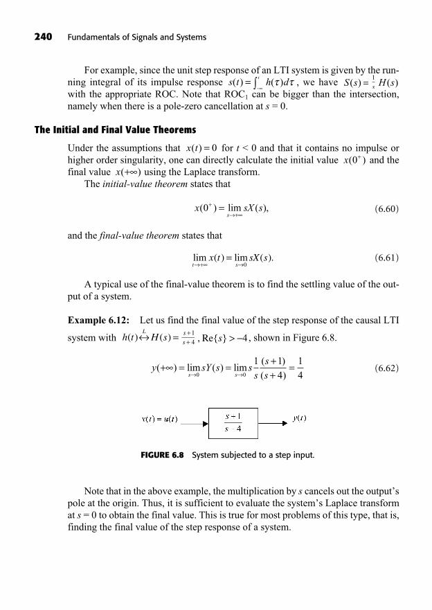
For example, since the unit step response of an LTI system is given by the run-ning integral of its impulse response , we have with the appropriate ROC. Note that ROC1 can be bigger than the intersection,namely when there is a pole-zero cancellation at s = 0.
The Initial and Final Value Theorems
Under the assumptions that for t < 0 and that it contains no impulse orhigher order singularity, one can directly calculate the initial value and thefinal value using the Laplace transform.
The initial-value theorem states that
(6.60)
and the final-value theorem states that
(6.61)
A typical use of the final-value theorem is to find the settling value of the out-put of a system.
Example 6.12: Let us find the final value of the step response of the causal LTI
system with , shown in Figure 6.8.
(6.62)y sY s ss
s
ss s( ) lim ( ) lim
( )
( )+ = =
++
=0 0
1 1
4
1
4
s, Re{ } > 4s
s
++
1
4h t H s
L( ) ( ) =
lim ( ) lim ( ).t s
x t sX s+
=0
x sX ss
( ) lim ( ),0+
+=
x( )+x( )0+
x t( ) = 0
H s( )s
1S s( ) =h d( )
ts t( ) =
240 Fundamentals of Signals and Systems
FIGURE 6.8 System subjected to a step input.
Note that in the above example, the multiplication by s cancels out the output’spole at the origin. Thus, it is sufficient to evaluate the system’s Laplace transformat s = 0 to obtain the final value. This is true for most problems of this type, that is,finding the final value of the step response of a system.

ANALYSIS AND CHARACTERIZATION OF LTI SYSTEMS USING THE LAPLACE TRANSFORM
We have seen that the convolution property makes the Laplace transform useful toobtain the response of an LTI system to an arbitrary input (with a Laplace trans-form). Specifically, the Laplace transform of the output of an LTI system with im-pulse response h(t) is simply given by
(6.63)
Also recall that the frequency response of the system is .
The Laplace transform H(s) of the impulse response is called the transfer func-tion. Many properties of LTI systems are associated with the characteristics oftheir transfer functions.
Causality
Recall that for for a causal system and thus is right-sided. Therefore,the ROC associated with the transfer function of a causal system is a right half-plane.
The converse is not true. For example, a right-sided signal starting at also leads to an ROC that is a right half-plane. However, if we know that the trans-fer function is rational, then it suffices to check that the ROC is the right half-planeto the right of the rightmost pole in the s-plane to conclude that the system iscausal.
Example 6.13: The transfer function corresponds to a
causal system. On the other hand, the transfer function is
noncausal (causal h(t) time-advanced by 1), whereas iscausal (causal h(t) time-delayed by 1).
Stability
So far, we have seen that bounded-input bounded-output (BIBO) stability of acontinuous-time LTI system is equivalent to its impulse response being absolutely integrable, in which case its Fourier transform converges. Also, the stability of anLTI differential system is equivalent to having all the zeros of its characteristicpolynomial having a negative real part.
For the Laplace transform, the first stability condition translates into the following:
An LTI system is stable if and only if the ROC of its transfer function containsthe j -axis.
s 1, Re{ }>e
s
s
1+H s2( ) =
s 1, Re{ }>e
s
s
1+H s1( ) =
s, Re{ }> 1s +1
1H s( ) =
t = 10
t < 0h t( ) = 0
H j H ss j
( ) ( )==
Y s H s X s( ) ( ) ( ), .= ROC ROC ROCY H X
The Laplace Transform 241
242 Fundamentals of Signals and Systems
Example 6.14: Consider an LTI system with proper transfer function:
(6.64)
Three possible ROCs could be associated with this transfer function. Table 6.1gives the impulse response for each ROC. Only one ROC leads to a stable system.Note that the system poles are marked with an X and the system zeros are markedwith an O in the s-plane.
First, let us compute the partial fraction expansion of H(s):
(6.65)
To obtain A, let : A = 1. Then, we find the coefficient B:
(6.66)
and finally we get coefficient C:
(6.67)
Hence, the transfer function can be expanded as
(6.68)
The first term is constant and corresponds to an impulse . The two otherterms are partial fractions that can correspond to right-sided or left-sided signals,depending on the chosen ROCs, as presented in Table 6.1.
The stability condition for a causal LTI system with a proper, rational trans-fer function is stated as follows. Note that a large class of causal differential LTIsystems have rational transfer functions.
A causal system with a proper rational transfer function H(s) is stable if andonly if all of its poles are in the left-half of the s-plane; that is, if all of the poleshave negative real parts.
( )t
H ss s
s s s s( )
( )
( )( ).=
++
= ++
1
2 11
2
3
1
1
2
3
1
2
Cs s
ss
=+
==
( )
( ).
1
1
2
32
Bs s
ss
=++
==
( )
( ),
1
2
2
31
s
H ss s
s sA
B
s
C
s( )
( )
( )( ).=
++
= + ++
1
2 1 1 2
H ss s
s s( )
( )
( )( ).=
++
1
2 1
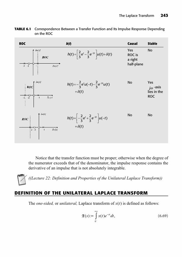
Notice that the transfer function must be proper; otherwise when the degree ofthe numerator exceeds that of the denominator, the impulse response contains thederivative of an impulse that is not absolutely integrable.
((Lecture 22: Definition and Properties of the Unilateral Laplace Transform))
DEFINITION OF THE UNILATERAL LAPLACE TRANSFORM
The one-sided, or unilateral, Laplace transform of x(t) is defined as follows:
(6.69)X ( ) : ( ) ,s x t e dtst=+
0
The Laplace Transform 243
ROC h(t) Causal Stable
Yes NoROC is a right half-plane
No Yes-axis
lies in theROC
No Noh t e e u t
t
t t( ) ( )
( )
= +
+
23
23
2
jh t e u t e u t
t
t t( ) ( ) ( )
( )
=
+
23
23
2
h t e e u t tt t( ) ( ) ( )= +23
23
2
TABLE 6.1 Correspondence Between a Transfer Function and Its Impulse Response Dependingon the ROC
where s is a complex variable. Notice that this transform considers only the sig-nal for nonnegative times. The lower limit of integration is , which meansthat singular functions such as impulses at t = 0 will be taken into account in theunilateral Laplace transform.
We will use the following notation for the unilateral Laplace transform:
(6.70)
Note that two signals that differ for t < 0 but are equal for will have thesame unilateral Laplace transform. Also note that the unilateral Laplace transformof x(t) is identical to the two-sided Laplace transform of , assuming thereis no impulse at t = 0. A direct consequence of this is that the Laplace transformproperties for causal, right-sided signals apply to the unilateral transform as well.Moreover, the ROC of a unilateral Laplace transform is always an open right half-plane or the entire s-plane.
PROPERTIES OF THE UNILATERAL LAPLACE TRANSFORM
The properties of the unilateral Laplace transform are identical to those of the reg-ular two-sided Laplace transform, except when time shifts are involved, which canmake part of the signal “disappear” to the negative times. Note that the followingproperties are summarized in Table D.6 of Appendix D.
Linearity
The unilateral Laplace transform is linear. If and
, then
(6.71)
Time Delay
For , if , then for a time delay of ,
(6.72)
Thus, for a time delay, this time-shifting property is exactly the same as that forthe two-sided Laplace transform. In the case where x(t) is nonzero at negative
x t t e s s tUL st( ) ( ), .>
0 00 0X ROC,
t0
0>x t s sUL
( ) ( ),X ROCx t t( ) ,= <0 0
ax t bx t a s b s sUL
1 2 1 2( ) ( ) ( ) ( ),+ +X X ROC ROC RO
1CC
2.
x t s sUL
2 2( ) ( ),X ROC
2
x t s sUL
1 1( ) ( ),X ROC
1
x t u t( ) ( )
t 0
x t s x tUL
( ) ( ) { ( )}.X =UL
t = 0
244 Fundamentals of Signals and Systems
times, a time delay can make a part of the signal “appear” at positive times, whichcould change the unilateral Laplace transform. For a time advance, the part of thesignal shifted to negative times is lost. In both of these cases there is no simple re-lationship between the resulting and the original unilateral transforms.
Shifting in the s-Domain
If , then
(6.73)
where the new ROC is the original one shifted by , to the right if this num-ber is positive, to the left otherwise.
Time Scaling
If , then for ,
(6.64)
where the new ROC is the original one, expanded or contracted by .
Conjugation
If , then
(6.75)
Therefore, for x(t) real, , and we have the important conse-quence that the complex poles and zeros of the unilateral Laplace transform of areal signal always come in conjugate pairs.
Convolution Property
Assume that . If and
, then
(6.76)
This is a useful property for causal LTI system analysis with signals that areidentically zero at negative times.
x t x t s s sUL
1 2 1 2( ) ( ) ( ) ( ), .X X ROC ROC ROC
1 2
x t s sUL
2 2( ) ( ),X ROC
2
x t s sUL
1 1( ) ( ),X ROC
1x t x t t
1 20 0( ) ( )= = < for
X X( ) ( )s s=
x t s sUL
( ) ( ),X ROC.
x t s sUL
( ) ( ),X ROC
1
x t s sUL
( ) ,( )1 1X ROC,
> 0x t s sUL
( ) ( ),X ROC
Re{ }s0
e x t s s ss t UL0
0( ) ( ), },X ROC+Re{s
0
x t s sUL
( ) ( ),X ROC
The Laplace Transform 245
Differentiation in the Time Domain
The differentiation property of the unilateral Laplace transform is particularly usefulfor analyzing the response of causal differential systems to nonzero initial conditions.
If , then
(6.77)
ROC1 can be larger than ROC when there is a pole-zero cancellation at s = 0.Note that the value is 0 for signals that are identically 0 for t < 0, but not forsignals that extend to negative times. Furthermore, can be used to set an ini-tial condition on the output of a causal differential system as shown in Example 6.15.
Example 6.15: Let us calculate the output of the following homogeneous causalLTI differential system with initial condition :
(6.78)
We take the unilateral Laplace transform on both sides:
(6.79)
Solving for Y(s), we obtain
(6.80)
which corresponds to the time-domain output signal:
(6.81)
Note that the unilateral Laplace transform of the -order derivative of x(t) isgiven by the following formula, which is derived by successive applications ofEquation 6.77.
(6.82)
d x t
dts s s x s
d x
dt
n
n
ULn n
n( )( ) ( )
( )X 1
2
00
…nn
n
n
d x
dts
2
1
1
0( ),
ROC ROC1
nth
y t y e u tt
( ) ( ) ( ).= 0 0
Y( )( )
, Re{ } ,sy
ss=
+>
01
1
00
00 0s s y sY Y( ) ( ) ( ) .+ =
00
dy t
dty t
( )( ) .+ =
y( )0
x( )0x( )0
dx t
dts s x s
UL( )( ) ( ),X 0 ROC ROC.
1
x t s sUL
( ) ( ),X ROC
246 Fundamentals of Signals and Systems
Differentiation in the Frequency Domain
If , then
(6.83)
Integration in the Time Domain
If , then
(6.84)
The Initial and Final Value Theorems
Even though these theorems were introduced as two-sided Laplace transform prop-erties, they are basically unilateral transform properties, as they apply only to sig-nals that are identically 0 for .
The initial-value theorem states that
(6.85)
and the final-value theorem states that
(6.86)
Example 6.16: Let us find the initial value of the signal whose unilat-eral Laplace transform is :
(6.87)
SUMMARY
In this chapter, we introduced the Laplace transform of a continuous-time signal asa generalization of the Fourier transform.
x s s sss s
( ) lim ( ) lim .010
310+
+ += = =X
, Re{ }s > 3s=
10
3X ( )s =x( )0+
lim ( ) lim ( ).s s
x t s s+
=0
X
x s ss
( ) lim ( ),0+
+= X
t < 0
x ds
s s s st UL
( ) ( ), :Re .0
1 { }X ROC ROC { }>01
x t s sUL
( ) ( ),X ROC
tx td s
dss
UL
( )( )
,X
ROC.
x t s sUL
( ) ( ),X ROC
The Laplace Transform 247
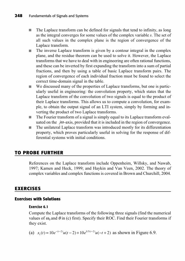
The Laplace transform can be defined for signals that tend to infinity, as longas the integral converges for some values of the complex variable s. The set ofall such values in the complex plane is the region of convergence of theLaplace transform.The inverse Laplace transform is given by a contour integral in the complexplane, and the residue theorem can be used to solve it. However, the Laplacetransforms that we have to deal with in engineering are often rational functions,and these can be inverted by first expanding the transform into a sum of partialfractions, and then by using a table of basic Laplace transform pairs. Theregion of convergence of each individual fraction must be found to select thecorrect time-domain signal in the table.We discussed many of the properties of Laplace transforms, but one is partic-ularly useful in engineering: the convolution property, which states that theLaplace transform of the convolution of two signals is equal to the product oftheir Laplace transforms. This allows us to compute a convolution, for exam-ple, to obtain the output signal of an LTI system, simply by forming and in-verting the product of two Laplace transforms.The Fourier transform of a signal is simply equal to its Laplace transform eval-uated on the -axis, provided that it is included in the region of convergence.The unilateral Laplace transform was introduced mostly for its differentiationproperty, which proves particularly useful in solving for the response of dif-ferential systems with initial conditions.
TO PROBE FURTHER
References on the Laplace transform include Oppenheim, Willsky, and Nawab,1997; Kamen and Heck, 1999; and Haykin and Van Veen, 2002. The theory ofcomplex variables and complex functions is covered in Brown and Churchill, 2004.
EXERCISES
Exercises with Solutions
Exercise 6.1
Compute the Laplace transforms of the following three signals (find the numericalvalues of 0 and in (c) first). Specify their ROC. Find their Fourier transforms ifthey exist.
(a) as shown in Figure 6.9.x t e u t e u tt t1
2 0 5 210 2 10 2( ) ( ) ( )( ) . ( )= + +
j
248 Fundamentals of Signals and Systems
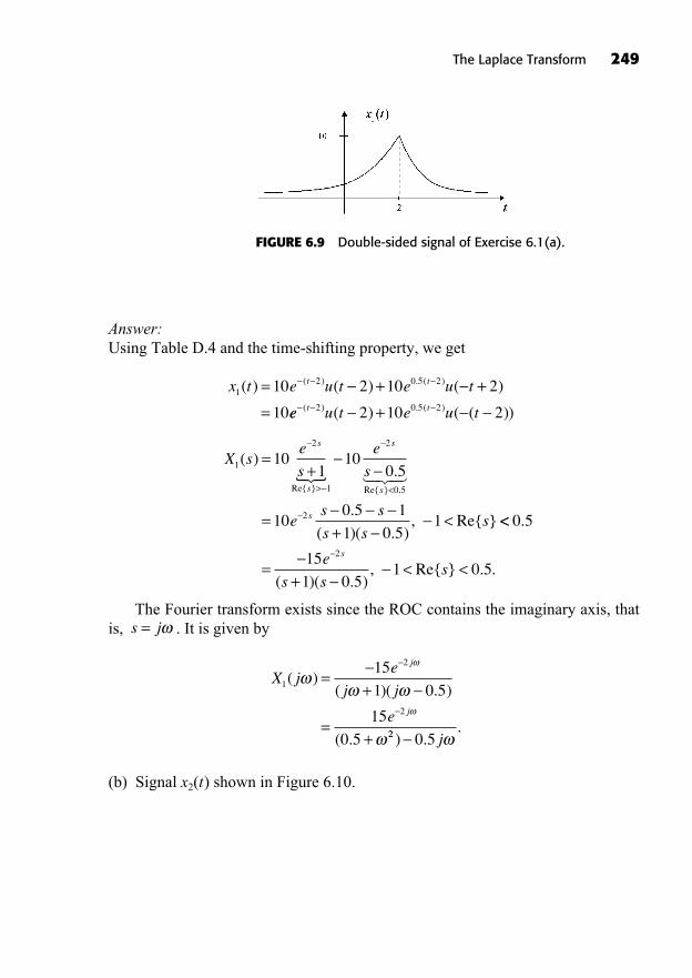
The Laplace Transform 249
Answer:Using Table D.4 and the time-shifting property, we get
The Fourier transform exists since the ROC contains the imaginary axis, thatis, . It is given by
(b) Signal x2(t) shown in Figure 6.10.
X je
j j
e
j
j
1
2
2
15
1 0 5
15
0 5
( )( )( . )
( .
=+
=+ 22 0 5) .
.j
s j=
X se
s
e
s
s
s
s
s
1
2
1
2
0
101
100 5
( ).
Re{ } Re{ }
=+> <�
..
.
( )( . ), Re{ }
5
2100 5 1
1 0 51
���
=+
<es s
s sss <<
=+
< <
0 5
15
1 0 51 0 5
2
.
( )( . ), Re{ } . .
e
s ss
s
x t e u t e u tt t1
2 0 5 210 2 10 2
10
( ) ( ) ( )( ) . ( )= + +
= ee u t e u tt t+( ) . ( )( ) ( ( ))2 0 5 22 10 2
FIGURE 6.9 Double-sided signal of Exercise 6.1(a).
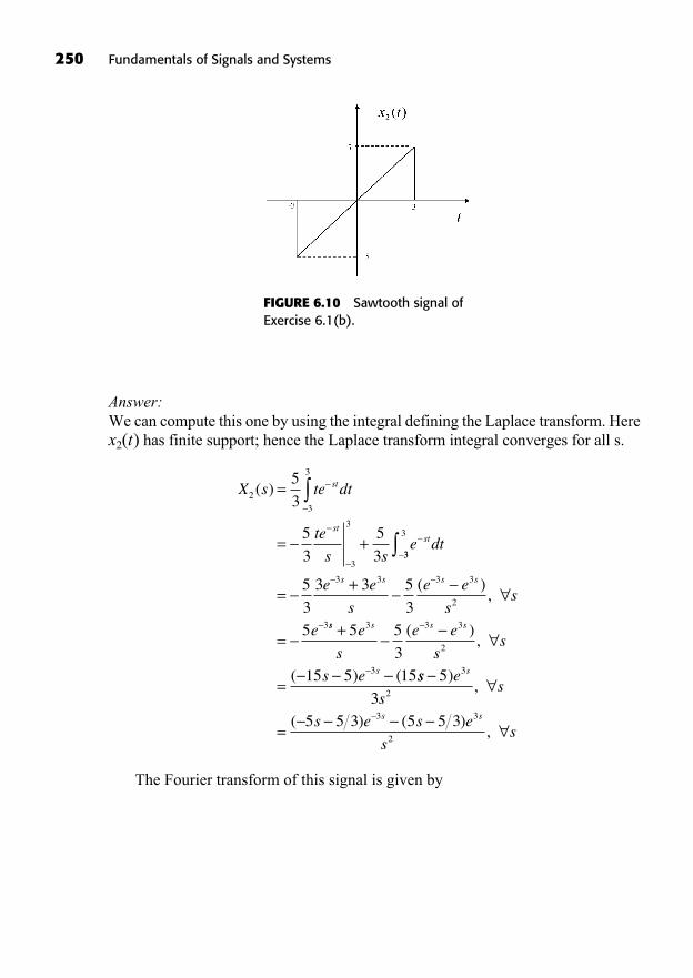
250 Fundamentals of Signals and Systems
Answer:We can compute this one by using the integral defining the Laplace transform. Herex2(t) has finite support; hence the Laplace transform integral converges for all s.
The Fourier transform of this signal is given by
X s te dt
te
s se dt
st
stst
2
3
3
3
3
5
3
5
3
5
3
( ) =
= +33
3
3 3 3 3
2
3
5
3
3 3 5
35
=+
=
e e
s
e e
ss
e
s s s s( ),
ss s s s
s
e
s
e e
ss
s e
+
=
5 5
315 5 15
3 3 3
2
3
( ),
( ) ( ss e
ss
s e s e
ss
s
s s
=
5
35 5 3 5 5 3
3
2
3 3
2
),
( ) ( ),
FIGURE 6.10 Sawtooth signal ofExercise 6.1(b).
It is odd and purely imaginary, as expected. Applying L’Hopital’s rule twice,we can also check that is finite, as it should be.
(c) Damped sinusoid signal of Figure 6.11.x t e t u tt3
100( ) sin( ) ( )= +
X j2 0( )
X jj e j e
j
j j
2
3 3
2
5 5 3 5 5 3
5
( )( ) ( )
(
=
=ee e e e
j e e
j j j j
j j
3 3 3 3
2
3 3
5 3
5
+ +
=+
) ( )
( ) ( )
cos( ) sin(=
5 3
10 3 10 3
3 3
2
e e
j j
j j
))
cos( ) sin( )3
103 3 3
3
2
2= j
The Laplace Transform 251
FIGURE 6.11 Damped sinusoid signal ofExercise 6.1(c).
Answer:Let us first find the values of the parameters and 0. We have
x3 0 0 5
0 5
6
( ) . sin( )
arcsin( . )
= ==
=
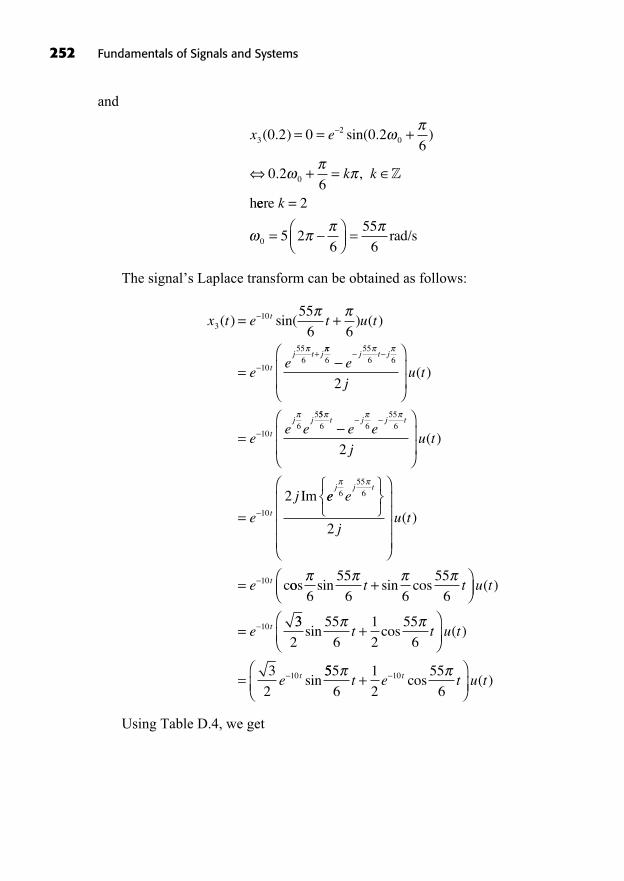
and
The signal’s Laplace transform can be obtained as follows:
Using Table D.4, we get
x t e t u t
ee
t
t
j t j
310
10
556
55
6 6( ) sin( ) ( )= +
=+
655
6 6
106
5
2
=
e
ju t
ee e
j t j
t
j j
( )
556 6
556
10
2
2
t j j t
t
e e
ju t
e
j
=
( )
Im ee e
ju t
e
j j t
t
655
6
10
2
=
( )
coos sin sin cos ( )6
55
6 6
55
6
10
t t u t
e t
+
=33
2
55
6
1
2
55
6
3
210
sin cos ( )
sin
t t u t
e t
+
= 555
6
1
2
55
610t e t u tt+ cos ( )
x e
k k
32
0
0
0 2 0 0 26
0 26
( . ) sin( . )
. ,
= = +
+ = Z
heere
rad/s
k =
= =
2
5 26
55
60
252 Fundamentals of Signals and Systems
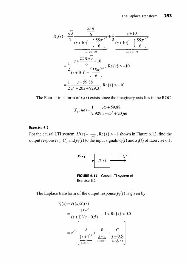
The Laplace Transform 253
The Fourier transform of x3(t) exists since the imaginary axis lies in the ROC.
Exercise 6.2
For the causal LTI system shown in Figure 6.12, find the
output responses y1(t) and y3(t) to the input signals x1(t) and x3(t) of Exercise 6.1.
s, Re{ } > 1s +
1
1H s( ) =
X jj
j3 2
1
2
59 88
929 3 20( )
.
.=
++
X s
s
s
32
2
10
3
2
556
1055
6
( )
( )
Re{ }
=+ +
>� ����� ���� �
++
+ +
>
1
2
10
1055
62
2
10
s
s
s
( )
Re{ }����� ����
=+ +
+ +
1
2
55 36
10
1055
62
2
s
s( )
, Ree{ }
.
., Re{ }
s
s
s ss
>
=+
+ +>
10
1
2
59 88
20 929 3102
FIGURE 6.12 Causal LTI system ofExercise 6.2.
The Laplace transform of the output response y1(t) is given by
Y s H s X s
e
s s
s
1 1
2
2
15
1 0 51
( ) ( ) ( )
( ) ( . ), Re{
=
=+
< ss
eA
s
B
ss
ss
} .
Re{ }Re{ }
<
=+( )
++
>>
0 5
1 12
2
1��� �� <
+
1 0 5
0 5� ���
C
ss
.Re{ } .
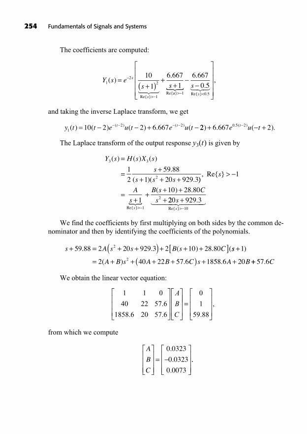
The coefficients are computed:
and taking the inverse Laplace transform, we get
The Laplace transform of the output response y3(t) is given by
We find the coefficients by first multiplying on both sides by the common de-nominator and then by identifying the coefficients of the polynomials.
We obtain the linear vector equation:
from which we compute
A
B
C
=0 0323
0 0323
0 0073
.
.
.
..
1 1 0
40 22 57 6
1858 6 20 57 6
.
. .
A
B
C
=0
1
59 88.
,
s A s s B s C+ = + +( ) + + +[ ]59 88 2 20 929 3 2 10 28 802. . ( ) . (ss
A B s A B C s A B
+
= + + + +( ) + +
1
2 40 22 57 6 1858 6 202
)
( ) . . ++ 57 6. C
Y s H s X s
s
s s s
3 3
2
1
2
59 88
1 20 929 3
( ) ( ) ( )
.
( )( .
=
=+
+ + + )), Re{ }
( ) .
Re{ }
s
A
s
B s C
ss
>
=+
++ ++
>
1
1
10 28 80
1
2� 220 929 3
10
ss
+>
.Re{ }
� ���� ����
y t t e u t e u tt t1
2 210 2 2 6 667( ) ( ) ( ) . (( ) ( )= + 22 6 667 20 5 2) . ( ).. ( )+ +e u tt
Y s es s
s
s
12
2
1
10
1
6 667
1( )
.
Re{ }Re{
=+( )
++
>��� �� ss s
s} Re{ } .
.
.,
> <1 0 5
6 667
0 5� ���
254 Fundamentals of Signals and Systems
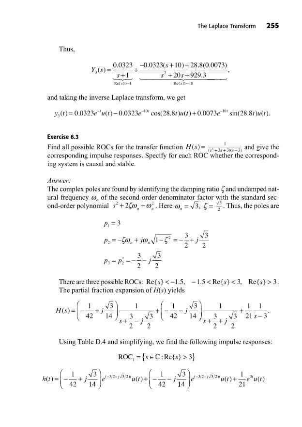
Thus,
and taking the inverse Laplace transform, we get
Exercise 6.3
Find all possible ROCs for the transfer function and give thecorresponding impulse responses. Specify for each ROC whether the correspond-ing system is causal and stable.
Answer:The complex poles are found by identifying the damping ratio and undamped nat-ural frequency n of the second-order denominator factor with the standard sec-ond-order polynomial . Here . Thus, the poles are
There are three possible ROCs: .The partial fraction expansion of H(s) yields
Using Table D.4 and simplifying, we find the following impulse responses:
h t j e u t jj t( ) ( )( )= + ++1
42
3
14
1
42
33 2 3 2
114
1
213 2 3 2 3+e u t e u tj t t( ) ( ) ( )
ROC1 3= >{ }s sC :Re{ }
H s j
s j
j( ) = ++
+1
42
3
14
1
32
32
1
42
3
14+ +
+1
32
32
1
21
1
3s j
s.
Re{ } . , . Re{ } , Re{ }s s s< < < >1 5 1 5 3 3
p
p j j
p p j
n n
1
22
3 2
3
13
2
3
2
3
2
3
2
=
= + = +
= =
=3
2n = =3,sn n
2 22+ +
s s s( )( )+ +1
3 3 32H s( ) =
y t e u t e t ut t3
100 0323 0 0323 28 8( ) . ( ) . cos( . ) (= tt e t u tt) . sin( . ) ( ).+ 0 0073 28 810
Y ss
s
s
3
1
0 0323
1
0 0323 10 28( )
. . ( )
Re{ }
=+
++ +
>���
.. ( . )
.Re{ }
8 0 0073
20 929 32
10
s ss
+ +>
� ������ �������,
The Laplace Transform 255
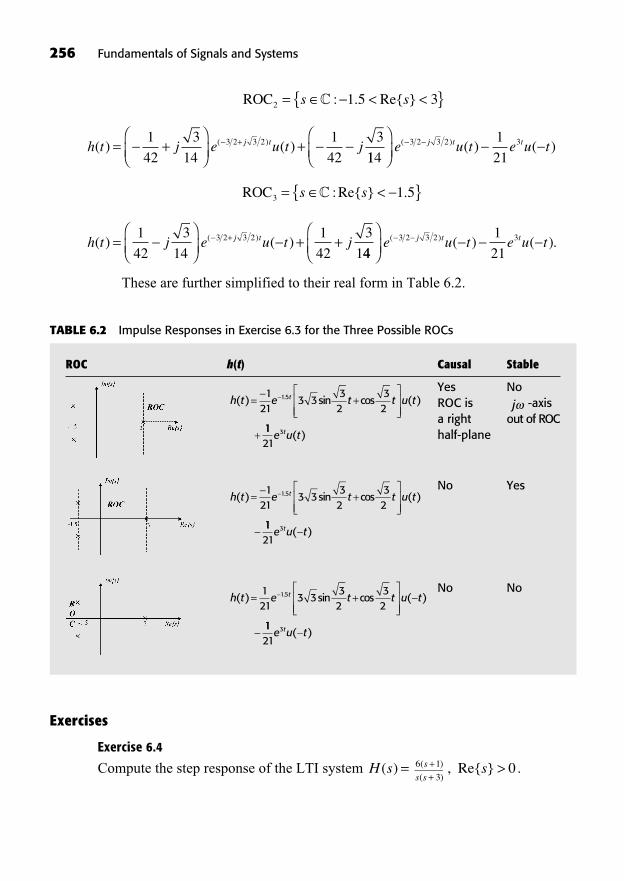
ROC h(t) Causal Stable
Yes NoROC is -axisa right out of ROChalf-plane
No Yes
No Noh t e t t u tt( ) sin cos ( ).= +1
213 3
32
32
15
1121
3e u tt ( )
h t e t t u tt( ) sin cos ( ).= +121
3 332
32
15
1121
3e u tt ( )
jh t e t t u tt( ) sin cos ( ).= +
+
121
3 332
32
15
1121
3e u tt ( )
TABLE 6.2 Impulse Responses in Exercise 6.3 for the Three Possible ROCs
These are further simplified to their real form in Table 6.2.
h t j e u t jj t( ) ( )( )= + ++1
42
3
14
1
42
3
13 2 3 2
44
1
213 2 3 2 3e u t e u tj t t( ) ( ) ( ).
ROC3 1 5= <{ }s sC :Re{ } .
h t j e u t jj t( ) ( )( )= + ++1
42
3
14
1
42
33 2 3 2
114
1
213 2 3 2 3e u t e u tj t t( ) ( ) ( )
ROC2 1 5 3= < <{ }s sC : . Re{ }
256 Fundamentals of Signals and Systems
Exercises
Exercise 6.4
Compute the step response of the LTI system .s, Re{ } > 0s
s s
( )
( )
++
6 1
3H s( ) =
Exercise 6.5
Compute the output y(t) of the LTI system for theinput signal .
Answer:
Exercise 6.6
Suppose that the LTI system described by is known to be stable.Is this system causal? Compute its impulse response h(t).
Exercise 6.7
Consider an LTI system with transfer function . Sketch all possibleregions of convergence of H(s) on pole-zero plots and compute the associated im-pulse responses h(t). Indicate for each impulse response whether it corresponds toa system that is causal/stable.
Answer:
Exercise 6.8
Consider an LTI system with transfer function . Sketch all possi-
ble ROCs of H(s) on a pole-zero plot and compute the associated impulse re-sponses h(t). Indicate for each impulse response whether it corresponds to a systemthat is causal/stable.
Exercise 6.9
Suppose we know that the input of an LTI system is . The outputwas measured to be . Find the transferfunction H(s) of the system and its ROC and sketch its pole-zero plot. Is the sys-tem causal? Is it stable? Justify your answers.
Answer:
y t e t u t e u t e u tt t t( ) sin( ) ( ) ( ) ( )= + + 2x t e u tt( ) ( )=
s s
s s
( )
+ +1
2 12H s( ) =
s s
s s+ +
2
2
2
5 6H s( ) =
s s( )( )+2
3 1H s( ) =
x t e u tt( ) ( )= 4s, Re{ } > 5
s s+ +100
10 1002H s( ) =
The Laplace Transform 257
Exercise 6.10
(a) Find the impulse response of the system ,. Hint: this system has a pole at –2.
(b) Find the settling value of the step response of H(s) given in (a).sRe{ } > 2
s s
s s s+ + +3 3 6
12 120 200
2
3 2H s( ) =
258 Fundamentals of Signals and Systems
259
Application of the Laplace Transform to LTI Differential Systems
7
In This Chapter
The Transfer Function of an LTI Differential SystemBlock Diagram Realizations of LTI Differential SystemsAnalysis of LTI Differential Systems With Initial Conditions Usingthe Unilateral Laplace TransformTransient and Steady-State Responses of LTI Differential SystemsSummaryTo Probe FurtherExercises
((Lecture 23: LTI Differential Systems and Rational Transfer Functions))
The Laplace transform is a powerful tool to solve linear time-invariant (LTI)differential equations. We have used the Fourier transform for the same pur-pose, but the Laplace transform, whether bilateral or unilateral, is applicable
in more cases, for example, to unstable systems or unbounded signals.
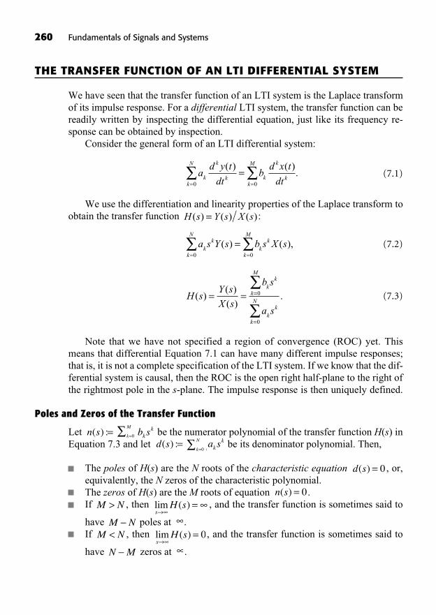
260 Fundamentals of Signals and Systems
THE TRANSFER FUNCTION OF AN LTI DIFFERENTIAL SYSTEM
We have seen that the transfer function of an LTI system is the Laplace transformof its impulse response. For a differential LTI system, the transfer function can bereadily written by inspecting the differential equation, just like its frequency re-sponse can be obtained by inspection.
Consider the general form of an LTI differential system:
(7.1)
We use the differentiation and linearity properties of the Laplace transform toobtain the transfer function :
(7.2)
(7.3)
Note that we have not specified a region of convergence (ROC) yet. Thismeans that differential Equation 7.1 can have many different impulse responses;that is, it is not a complete specification of the LTI system. If we know that the dif-ferential system is causal, then the ROC is the open right half-plane to the right ofthe rightmost pole in the s-plane. The impulse response is then uniquely defined.
Poles and Zeros of the Transfer Function
Let be the numerator polynomial of the transfer function H(s) inEquation 7.3 and let be its denominator polynomial. Then,
The poles of H(s) are the N roots of the characteristic equation , or,equivalently, the N zeros of the characteristic polynomial.The zeros of H(s) are the M roots of equation .If , then , and the transfer function is sometimes said to
have poles at . If , then , and the transfer function is sometimes said to
have zeros at . N M
lim ( )s
H s = 0M N<M N
lim ( )s
H s =M N>n s( ) = 0
d s( ) = 0
a skk
0k
N
=0d s( ) :=
b skk
k
M
=0n s( ) :=
H sY s
X s
b s
a s
kk
k
M
kk
k
N( )
( )
( ).= = =
=
0
0
a s Y s b s X sk
k
k
N
kk
k
M
( ) ( ),= =
=0 0
H s Y s X s( ) ( ) ( )=
ad y t
dtb
d x t
dtk
k
kk
N
k
k
kk
M( ) ( ).
= =
=0 0
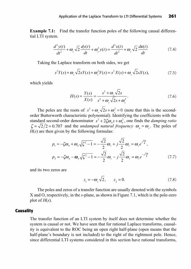
Example 7.1: Find the transfer function poles of the following causal differen-tial LTI system.
(7.4)
Taking the Laplace transform on both sides, we get
(7.5)
which yields
(7.6)
The poles are the roots of (note that this is the second-order Butterworth characteristic polynomial). Identifying the coefficients with thestandard second-order denominator , one finds the damping ratio
and the undamped natural frequency . The poles ofH(s) are then given by the following formulas:
(7.7)
and its two zeros are
(7.8)
The poles and zeros of a transfer function are usually denoted with the symbolsX and O, respectively, in the s-plane, as shown in Figure 7.1, which is the pole-zeroplot of H(s).
Causality
The transfer function of an LTI system by itself does not determine whether thesystem is causal or not. We have seen that for rational Laplace transforms, causal-ity is equivalent to the ROC being an open right half-plane (open means that thehalf-plane’s boundary is not included) to the right of the rightmost pole. Hence,since differential LTI systems considered in this section have rational transforms,
z zc1 2
2 0= =, .
p j e
p
n n c c c
j
n
12
34
2
12
2
2
2= + = + =
=
,
n c c c
jj e2
341
2
2
2
2= =
n c== =2 2 0 707.
s sn n2 22+ +
s sc c
2 22 0+ + =
H sY s
X s
s s
s sc
c c
( )( )
( ).= =
+
+ +
2
2 2
2
2
s Y s sY s Y s s X s sX sc c c
2 2 22 2( ) ( ) ( ) ( ) ( ),+ + = +
d y t
dt
dy t
dty t
d x t
dt
dc c c
2
2
22
22 2
( ) ( )( )
( )+ + = +
xx t
dt
( )
Application of the Laplace Transform to LTI Differential Systems 261
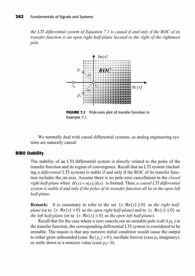
262 Fundamentals of Signals and Systems
the LTI differential system of Equation 7.1 is causal if and only if the ROC of itstransfer function is an open right half-plane located to the right of the rightmostpole.
FIGURE 7.1 Pole-zero plot of transfer function inExample 7.1.
We normally deal with causal differential systems, as analog engineering sys-tems are naturally causal.
BIBO Stability
The stability of an LTI differential system is directly related to the poles of thetransfer function and its region of convergence. Recall that an LTI system (includ-ing a differential LTI system) is stable if and only if the ROC of its transfer func-tion includes the j -axis. Assume there is no pole-zero cancellation in the closedright half-plane when is formed. Then, a causal LTI differentialsystem is stable if and only if the poles of its transfer function all lie in the open lefthalf-plane.
Remark: It is customary to refer to the set as the right half-plane (or to as the open right half-plane) and to asthe left half-plane (or to as the open left half-plane).
Recall that for the case where a zero cancels out an unstable pole (call it p0 ) inthe transfer function, the corresponding differential LTI system is considered to beunstable. The reason is that any nonzero initial condition would cause the output to either grow unbounded (case ), oscillate forever (case p0 imaginary),or settle down to a nonzero value (case p0= 0).
Re{ }p0
0>
{ :Re{ } }s s < 0{ :Re{ } }s s 0{ :Re{ } }s s > 0
{ :Re{ } }s s 0
H s n s d s( ) ( ) ( )=
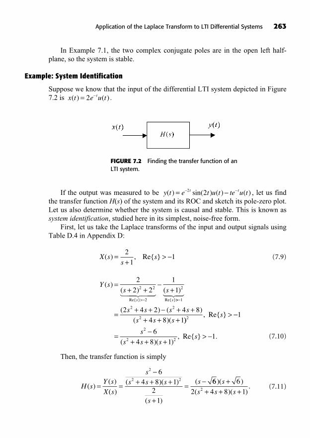
In Example 7.1, the two complex conjugate poles are in the open left half-plane, so the system is stable.
Example: System Identification
Suppose we know that the input of the differential LTI system depicted in Figure7.2 is .x t e u tt( ) ( )= 2
Application of the Laplace Transform to LTI Differential Systems 263
FIGURE 7.2 Finding the transfer function of anLTI system.
If the output was measured to be , let us findthe transfer function H(s) of the system and its ROC and sketch its pole-zero plot.Let us also determine whether the system is causal and stable. This is known assystem identification, studied here in its simplest, noise-free form.
First, let us take the Laplace transforms of the input and output signals usingTable D.4 in Appendix D:
(7.9)
(7.10)
Then, the transfer function is simply
(7.11)H sY s
X s
ss s s
s
s( )
( )
( )( )( )
( )
(= = + + +
+
=
2
2 2
64 8 1
21
66 6
2 4 8 12
)( )
( )( ).
s
s s s
++ + +
Y ss s
s s
( )( ) ( )
Re{ } Re{ }
=+ + +
>
2
2 2
1
12 2
2
2
� ��� ���>>
=+ + + +
+ + +
1
2 2
2
2 4 2 4 8
4 8 1
��� ��
( ) ( )
( )(
s s s s
s s s )), Re{ }
( )( ), Re{ } .
2
2
2 2
1
6
4 8 11
s
s
s s ss
>
=+ + +
>
X ss
s( ) , Re{ }=+
>2
11
y t e t u t te u tt t( ) sin( ) ( ) ( )= 2 2
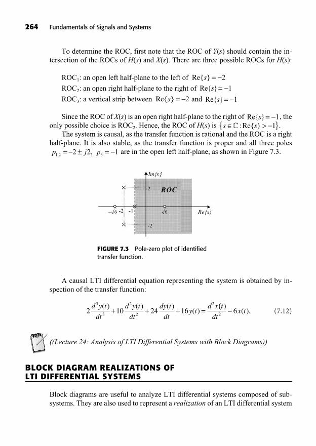
264 Fundamentals of Signals and Systems
To determine the ROC, first note that the ROC of Y(s) should contain the in-tersection of the ROCs of H(s) and X(s). There are three possible ROCs for H(s):
ROC1: an open left half-plane to the left of
ROC2: an open right half-plane to the right of
ROC3: a vertical strip between and
Since the ROC of X(s) is an open right half-plane to the right of , theonly possible choice is ROC2. Hence, the ROC of H(s) is .
The system is causal, as the transfer function is rational and the ROC is a righthalf-plane. It is also stable, as the transfer function is proper and all three poles
are in the open left half-plane, as shown in Figure 7.3.p j p1 2 32 2 1, ,= ± =
s s >{ }C :Re{ } 1Re{ }s = 1
Re{ }s = 1Re{ }s = 2
Re{ }s = 1
Re{ }s = 2
FIGURE 7.3 Pole-zero plot of identifiedtransfer function.
A causal LTI differential equation representing the system is obtained by in-spection of the transfer function:
(7.12)
((Lecture 24: Analysis of LTI Differential Systems with Block Diagrams))
BLOCK DIAGRAM REALIZATIONS OF LTI DIFFERENTIAL SYSTEMS
Block diagrams are useful to analyze LTI differential systems composed of sub-systems. They are also used to represent a realization of an LTI differential system
2 10 24 163
3
2
2
2d y t
dt
d y t
dt
dy t
dty t
d x( ) ( ) ( )( )+ + + =
(( )( ).
t
dtx t2 6
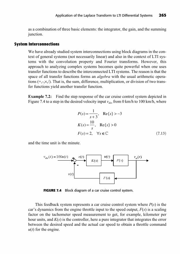
as a combination of three basic elements: the integrator, the gain, and the summingjunction.
System Interconnections
We have already studied system interconnections using block diagrams in the con-text of general systems (not necessarily linear) and also in the context of LTI sys-tems with the convolution property and Fourier transforms. However, thisapproach to analyzing complex systems becomes quite powerful when one usestransfer functions to describe the interconnected LTI systems. The reason is that thespace of all transfer functions forms an algebra with the usual arithmetic opera-tions (+,-,×,/). That is, the sum, difference, multiplication, or division of two trans-fer functions yield another transfer function.
Example 7.2: Find the step response of the car cruise control system depicted inFigure 7.4 to a step in the desired velocity input vdes from 0 km/h to 100 km/h, where
(7.13)
and the time unit is the minute.
P ss
s
K ss
s
F s s
( ) , Re{ }
( ) , Re{ }
( ) ,
=+
>
= >
=
1
33
100
2 �
Application of the Laplace Transform to LTI Differential Systems 265
FIGURE 7.4 Block diagram of a car cruise control system.
This feedback system represents a car cruise control system where P(s) is thecar’s dynamics from the engine throttle input to the speed output, F(s) is a scalingfactor on the tachometer speed measurement to get, for example, kilometer perhour units, and K(s) is the controller, here a pure integrator that integrates the errorbetween the desired speed and the actual car speed to obtain a throttle commandu(t) for the engine.
It is interesting to note that the theory of Laplace transforms and transfer func-tions allows us to analyze within a single framework a mechanical system (the car),an electromechanical sensor (the tachometer), and a control circuit or a control al-gorithm residing in a microcontroller chip.
The first task of a control engineer would be to check that this system is stable.We do not want the car to accelerate out of control when the driver switches thecruise control system on. Thus, we need to find the transfer function relating theinput vdes(t) to the scaled measured speed of the car v(t) and compute its poles. Letus denote the Laplace transforms of the signals with “hats.” We have
(7.14)
Thus, the error can be expressed as
(7.15)
and substituting this expression back into the first equation of Equation 7.14, weobtain
(7.16)
This is the transfer function relating the desired car velocity to its measure-ment. Using the actual transfer functions provided above, we get
(7.17)
This is a second-order transfer function with undamped natural frequency
rad/min and damping ratio . Hence, the poles are in theopen left-half plane:
(7.18)
p j
p
n n
n n
12
22
1 1 5 4 2131
1
= + = +
= =
. .
11 5 4 2131. . ,j
= 0 34.3
2 20=
n= 20
H ss s
s s
s s
( ) .=+
=+ +
+
+
2
1 2
20
3 20
13
10
13
10 2
ˆ( )( ) ( ) ( )
( ) ( ) ( )( )
v sF s P s K s
F s P s K sH s
=+1� ���� �����
ˆ ( ) ( ) ˆ ( ).v s H s v sdes des=
ˆ( ) ˆ ( ) ( ) ( ) ( ) ˆ( )
( ) (
e s v s F s P s K s e s
F s P s
des=
=+
1
1 )) ( )ˆ ( ).
K sv s
des
ˆ( ) ( ) ( ) ( ) ˆ( )
ˆ( ) ˆ ( ) ˆ( )
v s F s P s K s e s
e s v s v sdes
== ..
266 Fundamentals of Signals and Systems
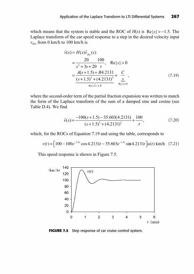
Application of the Laplace Transform to LTI Differential Systems 267
which means that the system is stable and the ROC of H(s) is . TheLaplace transform of the car speed response to a step in the desired velocity inputvdes from 0 km/h to 100 km/h is
(7.19)
where the second-order term of the partial fraction expansion was written to matchthe form of the Laplace transform of the sum of a damped sine and cosine (seeTable D.4). We find
(7.20)
which, for the ROCs of Equation 7.19 and using the table, corresponds to
(7.21)
This speed response is shown in Figure 7.5.
v t e t et t( ) cos . . si. .= 100 100 4 2131 35 6031 5 1 5 nn . ( )4 2131t u t km/h
ˆ( )( . ) . ( . )
( . ) (v s
s
s=
++ +
100 1 5 35 603 4 2131
1 5 42 .. ),
2131
1002
+s
ˆ( ) ( ) ˆ ( )
, Re{ }
v s H s v s
s s ss
A
des=
=+ +
>
=
20
3 20
1000
2
(( . ) .
( . ) ( . )Re{ } .
s B
ss
+ ++ +
>
1 5 4 2131
1 5 4 21312 2
1 550
� ���� ���� �+
>
C
ssRe{ }
,
Re{ } .s > 1 5
FIGURE 7.5 Step response of car cruise control system.
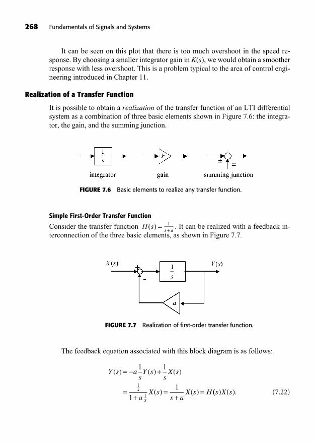
268 Fundamentals of Signals and Systems
It can be seen on this plot that there is too much overshoot in the speed re-sponse. By choosing a smaller integrator gain in K(s), we would obtain a smootherresponse with less overshoot. This is a problem typical to the area of control engi-neering introduced in Chapter 11.
Realization of a Transfer Function
It is possible to obtain a realization of the transfer function of an LTI differentialsystem as a combination of three basic elements shown in Figure 7.6: the integra-tor, the gain, and the summing junction.
FIGURE 7.6 Basic elements to realize any transfer function.
Simple First-Order Transfer Function
Consider the transfer function . It can be realized with a feedback in-terconnection of the three basic elements, as shown in Figure 7.7.
s a+1H s( ) =
FIGURE 7.7 Realization of first-order transfer function.
The feedback equation associated with this block diagram is as follows:
(7.22)
Y s asY s
sX s
aX s
s aX s Hs
s
( ) ( ) ( )
( ) ( )
= +
=+
=+
=
1 1
1
11
1(( ) ( ).s X s

With this simple block diagram, we can realize any transfer function of anyorder after it is written as a partial fraction expansion. This leads to the parallelform introduced below.
Simple Second-Order Transfer Function
Consider the transfer function . It can be realized with a feedbackinterconnection of the three basic elements in a number of ways. One way is to ex-pand the transfer function as a sum of two first-order transfer functions (partialfraction expansion). The resulting form is called the parallel form and is discussedbelow. Another way is to break up the transfer function as a cascade (multiplica-tion) of two first-order transfer functions. This cascade form is also discussedbelow. Yet another way to realize the second-order transfer function is the so-called direct form or controllable canonical form. To develop this form, considerthe system equation
(7.23)
This equation can be realized as in Figure 7.8. The idea is that the variable atthe input of an integrator is thought of as the derivative of its output.
s Y s a sY s a Y s X s21 0
( ) ( ) ( ) ( ).= +
s a s a+ +1
21 0
H s( ) =
Application of the Laplace Transform to LTI Differential Systems 269
FIGURE 7.8 Direct form realization of a second-order transferfunction.
Parallel Realization
A parallel realization can be obtained by expanding the transfer function intopartial first-order fractions with real coefficients or complex coefficients for com-plex poles.
Example 7.3: Consider the system . Its parallel re-alization is shown in Figure 7.9.
s 2
13+
s +1
23=s
s s( )( )+1
1 2H s( ) =
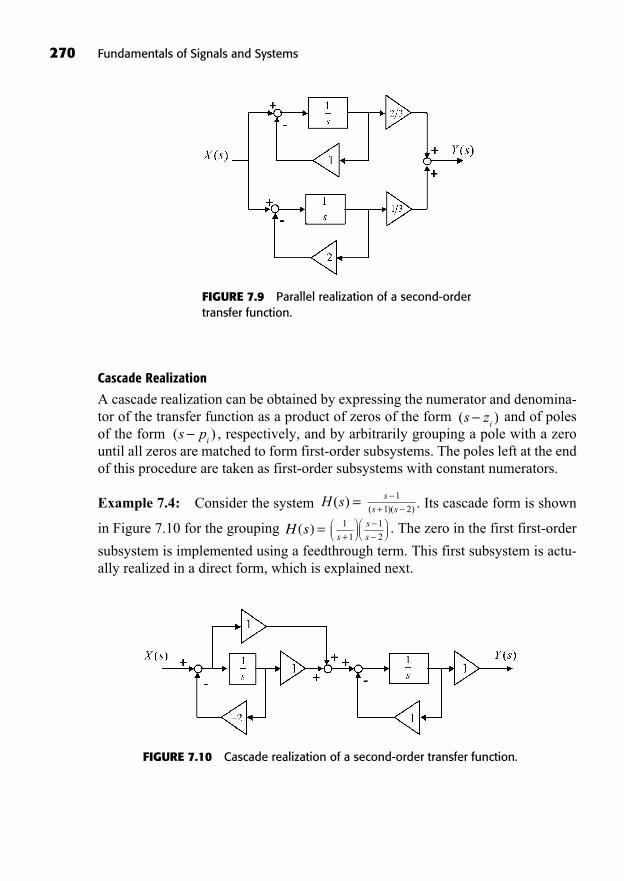
270 Fundamentals of Signals and Systems
Cascade Realization
A cascade realization can be obtained by expressing the numerator and denomina-tor of the transfer function as a product of zeros of the form and of polesof the form , respectively, and by arbitrarily grouping a pole with a zerountil all zeros are matched to form first-order subsystems. The poles left at the endof this procedure are taken as first-order subsystems with constant numerators.
Example 7.4: Consider the system . Its cascade form is shown
in Figure 7.10 for the grouping . The zero in the first first-order
subsystem is implemented using a feedthrough term. This first subsystem is actu-ally realized in a direct form, which is explained next.
s
s
s+1
1
1
2H s( ) =
s
s s( )( )+1
1 2H s( ) =
( )s pi
( )s zi
FIGURE 7.9 Parallel realization of a second-ordertransfer function.
FIGURE 7.10 Cascade realization of a second-order transfer function.
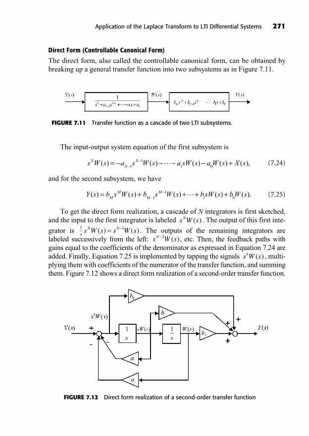
Direct Form (Controllable Canonical Form)
The direct form, also called the controllable canonical form, can be obtained bybreaking up a general transfer function into two subsystems as in Figure 7.11.
Application of the Laplace Transform to LTI Differential Systems 271
FIGURE 7.11 Transfer function as a cascade of two LTI subsystems.
The input-output system equation of the first subsystem is
(7.24)
and for the second subsystem, we have
(7.25)
To get the direct form realization, a cascade of N integrators is first sketched,and the input to the first integrator is labeled . The output of this first inte-
grator is . The outputs of the remaining integrators are labeled successively from the left: , etc. Then, the feedback paths withgains equal to the coefficients of the denominator as expressed in Equation 7.24 areadded. Finally, Equation 7.25 is implemented by tapping the signals , multi-plying them with coefficients of the numerator of the transfer function, and summingthem. Figure 7.12 shows a direct form realization of a second-order transfer function.
s W sk ( )
s W sN 2 ( )
1s W s s W sN N( ) ( )=1
s
s W sN ( )
Y s b s W s b s W s b sW s b W sM
MM
M( ) ( ) ( ) ( ) ( )= + + + +1
11 0
..
s W s a s W s a sW s a W s X sNN
N( ) ( ) ( ) ( ) ( ),= +1
11 0
FIGURE 7.12 Direct form realization of a second-order transfer function
((Lecture 25: Response of LTI Differential Systems with Initial Conditions))
ANALYSIS OF LTI DIFFERENTIAL SYSTEMS WITH INITIALCONDITIONS USING THE UNILATERAL LAPLACE TRANSFORM
Recall the differentiation property of the unilateral Laplace transform:
If , then
(7.26)
We have already solved a first-order system with an initial condition. Let usnow look at a second-order LTI differential system with initial conditions and anonzero input.
Example 7.5: Consider the causal second-order system described by
(7.27)
and with initial conditions . Suppose that this system is sub-jected to the input signal:
(7.28)
What is the output of the system? Take the unilateral Laplace transform onboth sides of Equation 7.27.
(7.29)
Note that . Collecting the terms containing Y(s) on the left-hand sideand putting everything else on the right-hand side, we can solve for Y(s).
(7.30)
s s s s s sy ydy2 3 2 3 0 3 0
0+ +( ) = +( ) + + +Y X( ) ( ) ( ) ( )
( ))
( )( ) ( ) ( )
(dt
ss s
s s
sy ydy
YX
=+( )+ +
++ +3
3 2
0 3 0
2
00
3 22 + +
)dt
s s
x( )0 0=
s s sydy
dts s y2 0
03 0Y Y( ) ( )
( )( ) ( )+ + = +2 0 3Y X X( ) ( ) ( ) ( )s s s x s
x t e u tt( ) ( ).= 5
y, ( )2 0 1= =dy
dt
( )0
d y t
dt
dy t
dty t
dx t
dtx t
2
23 2 3
( ) ( )( )
( )( )+ + = +
dx t
dts s x s
UL( )( ) ( ),X 0 ROC ROC.
1
x t s sUL
( ) ( ),X ROC
272 Fundamentals of Signals and Systems
We have,
(7.31)
and thus,
(7.32)
Taking the inverse Laplace transform of each term, we obtain
(7.33)
Zero-Input Response and Zero-State Response
The response of a causal LTI differential system with initial conditions and anonzero input can be decomposed as the sum of a zero-input response and a zero-state response. As these names imply, the zero-input response is due to the initialconditions only, whereas the zero-state response is produced by the input only.Note that the term state refers to the initial state in a state-space description of a dif-ferential system. We will study state-space systems in Chapter 10.
In Example 7.5, the zero-input and zero-state responses in the Laplace domainare identified as follows.
(7.34)YX
( )( )
ss s
s s=
+( )+ +
+3
3 22
zero-state resp.� �� ��
ssy ydydt
s s
( ) ( )( )
0 3 00
3 22
+ +
+ +zero-input ressp.
� ����� �����
y t e e e u tt t t( ) ( ).=9
2
10
3
1
62 5
Y( ) , Re{ }ss
s s s
s
s ss=
++ +( ) +( )
++
+ +>
=
3
3 2 5
5
3 21
2 2
ss s
s s ss
s
2
2
92
103
11 28
3 2 51
1
+ ++ +( ) +( )
>
=+
, Re{ }
ss s+ +2 5
16 .
X ( ) , Re{ } ,ss
s=+
>1
55
Application of the Laplace Transform to LTI Differential Systems 273
TRANSIENT AND STEADY-STATE RESPONSES OF LTI DIFFERENTIAL SYSTEMS
The transient response (also called natural response) of a causal, stable LTI dif-ferential system is the homogeneous response.
The steady-state response (or forced response) is the particular solution corre-sponding to a constant or periodic input. We say that a stable system is in steady-state when the transient component of the output has practically disappeared. Forexample, consider the step response
(7.35)
The transient part of this response is the term , and the steady-state partis u(t).
As another example, assume that a causal LTI differential system is subjected tothe sinusoidal input signal . Suppose that the resulting output is
(7.36)
Then the transient response of the system to the input is ,while is the steady-state response.
The steady-state response of a causal, stable LTI system to a sinusoidal inputof frequency 0 is also a sinusoid of frequency 0, although in general with a dif-ferent amplitude and phase.
Transient and Steady-State Analysis Using the Laplace Transform
For a causal, stable LTI system with a real-rational transfer function, a partial frac-tion expansion of the transfer function allows us to determine which terms corre-spond to transients (the terms with the system poles) and which correspond to thesteady-state response (terms with the input poles).
Example 7.6: Consider the step response.
(7.37)
Y ss
s sX s s
s
s s
( ) ( ), Re{ }=+
+ +( ) >
=+
+ +( )
3
3 21
3
3 2
2
2 sss
A
s
B
s
C
ss s
, Re{ }
Re{ } Re{ } Re
>
=+
++
+
> >
0
1 21 2� �
{{ }s >0�
20
sin( ) ( )t u te t u tt +2 2cos( ) ( )
y t t u t e t u tt( ) sin( ) ( ) cos( ) ( ).= + +2 20
2
x t t u t( ) sin( ) ( )=0
e u tt5 ( )
s t u t e u tt( ) ( ) ( ).= 5
274 Fundamentals of Signals and Systems
The steady-state response corresponds to the last term, C, which in the time-domain is Cu(t). The other two terms correspond to the transient response
.If we are only interested in the steady-state response of an LTI system, there is
no need to do a partial fraction expansion. The transfer function and the frequencyresponse of the system (which is the transfer function evaluated at s = j ) directlygive us the answer.
Step Response
We can use the final value theorem to determine the steady-state component of astep response. In general, this component is a step function Au(t). The “gain” A isgiven by
(7.38)
Response to a Sinusoid or a Periodic Complex Exponential
The frequency response of the system directly gives us the steady-state response toa sinusoid or a periodic complex exponential signal. For the latter, ,the steady-state response is
(7.39)
For a sinusoidal input, say , the steady-state response is as fol-lows (the same for a cosine signal):
(7.40)
where we used the fact that the frequency response magnitude is even and the phaseis odd for a real-rational transfer function. An important application is the steady-state analysis of circuits at a fixed frequency, for instance, 60 Hz. For example, if a
y tA
jH j e H j e
A
jH
ssj t j t( ) ( ( ) ( ) )
(
=
=
2
2
0 00 0
(( ) ( )( ( )) ( (j e H j ej t H j j t H j0 0
0 0 0+ 00
0 0
2 0 0
))
( ( )) (
)
( ( ) ( )= +A
jH j e H j ej t H j j 00 0
0 0 0
t H j
H j A t H j
+
= +( )
( )) )
( ) sin ( ) ,
x t A t( ) sin( )=0
y t H j Ae
H j Ae
ss
j t
j t H j
( ) ( )
( ) .( )
=
= +( )0
0
0
0 0
x t Ae j t( ) = 0
A sH ss
Hs
= =lim ( ) ( )0
10
Ae u t Be u tt t+( ) ( )2
Application of the Laplace Transform to LTI Differential Systems 275
circuit is described by its impedance, Z(s), seen as a transfer function, then itssteady-state response to a 60 Hz sinusoidal current is characterized by the complexnumber .
Response to a Periodic Signal
Again, the frequency response of the system gives us the steady-state response toa periodic signal admitting a Fourier series representation. For ,the steady-state response is the periodic signal:
(7.41)
SUMMARY
In this chapter, we studied the application of the Laplace transform to differentialsystems.
The transfer function of an LTI differential system can be obtained by inspec-tion of the differential equation.The zeros and poles of a transfer function were defined as the zeros of its nu-merator and denominator, respectively.Transfer functions can be interconnected in block diagrams to form more com-plex systems whose transfer functions can be obtained using simple rules.Any proper real-rational transfer function can be realized using an intercon-nection of three basic elements: the gain, the summing junction, and the inte-grator. We discussed the parallel, cascade, and direct form realizations.The unilateral Laplace transform can be used to compute the response of a dif-ferential system with initial conditions. The overall response is composed of azero-state response coming from the input only (assuming zero initial condi-tions) and of a zero-input response caused by the initial conditions only. An-other way to decompose the overall response of the system is to identify thetransient response and the steady-state response.
TO PROBE FURTHER
On the response of LTI differential systems, see, for example, Oppenheim, Will-sky, and Nawab, 1997. We will revisit realization theory in the context of state-space systems in Chapter 10.
y t H jk a ess k
jk t
k
( ) ( ) .==
+
00
a ek
jk t0
k=
+
x t( ) =
Z j( )2 60
276 Fundamentals of Signals and Systems
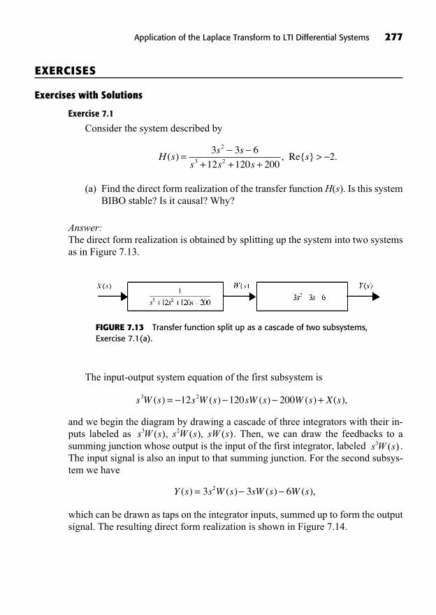
Application of the Laplace Transform to LTI Differential Systems 277
EXERCISES
Exercises with Solutions
Exercise 7.1
Consider the system described by
(a) Find the direct form realization of the transfer function H(s). Is this systemBIBO stable? Is it causal? Why?
Answer:The direct form realization is obtained by splitting up the system into two systemsas in Figure 7.13.
H ss s
s s ss( ) , Re{ } .=
+ + +>
3 3 6
12 120 2002
2
3 2
FIGURE 7.13 Transfer function split up as a cascade of two subsystems,Exercise 7.1(a).
The input-output system equation of the first subsystem is
and we begin the diagram by drawing a cascade of three integrators with their in-puts labeled as . Then, we can draw the feedbacks to asumming junction whose output is the input of the first integrator, labeled .The input signal is also an input to that summing junction. For the second subsys-tem we have
which can be drawn as taps on the integrator inputs, summed up to form the outputsignal. The resulting direct form realization is shown in Figure 7.14.
Y s s W s sW s W s( ) ( ) ( ) ( ),= 3 3 62
s W s3 ( )s W s s W s sW s3 2( ), ( ), ( )
s W s s W s sW s W s X s3 212 120 200( ) ( ) ( ) ( ) ( ),= +
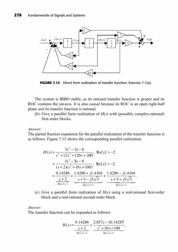
278 Fundamentals of Signals and Systems
The system is BIBO stable, as its rational transfer function is proper and itsROC contains the j -axis. It is also causal because its ROC is an open right-halfplane and its transfer function is rational.
(b) Give a parallel form realization of H(s) with (possibly complex-rational)first-order blocks.
Answer:The partial fraction expansion for the parallel realization of the transfer function isas follows. Figure 7.15 shows the corresponding parallel realization.
(c) Give a parallel form realization of H(s) using a real-rational first-orderblock and a real-rational second-order block.
Answer:The transfer function can be expanded as follows:
H ss
s
s
( ). . .
Re{ }
=+
+
>
0 14286
2
2 857 10 1428
2��� ��
77
10 1002
5
s ss
+ +>Re{ }
,� ���� ����
H ss s
s s ss
s
( ) , Re{ }=+ + +
>
=
3 3 6
12 120 2002
3
2
3 2
2 33 6
2 10 1002
0 14286
2
2
s
s s ss
s
+ + +>
=+
( )( ), Re{ }
.
Ree{ } Re{ }
. .
s s
j
s j> >
++
+2 5
1 4286 1 4104
5 5 3��� �� �� ���� ���� � ��+
+ +>
1 4286 1 4104
5 5 35
. .
Re{ }
j
s js
��� ����.
FIGURE 7.14 Direct form realization of transfer function, Exercise 7.1(a).
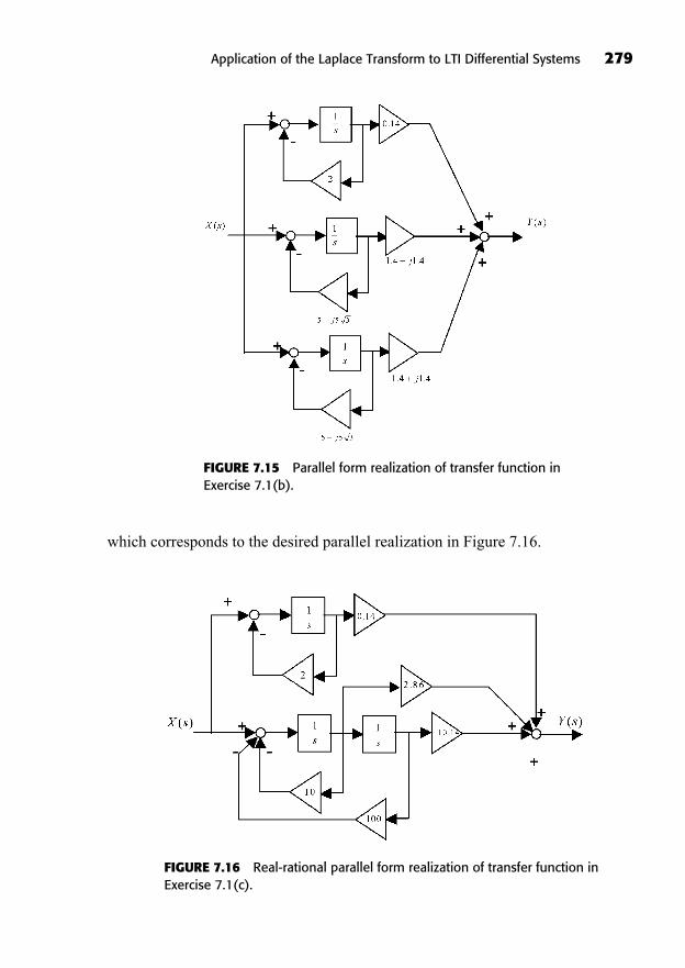
which corresponds to the desired parallel realization in Figure 7.16.
Application of the Laplace Transform to LTI Differential Systems 279
FIGURE 7.15 Parallel form realization of transfer function inExercise 7.1(b).
FIGURE 7.16 Real-rational parallel form realization of transfer function inExercise 7.1(c).
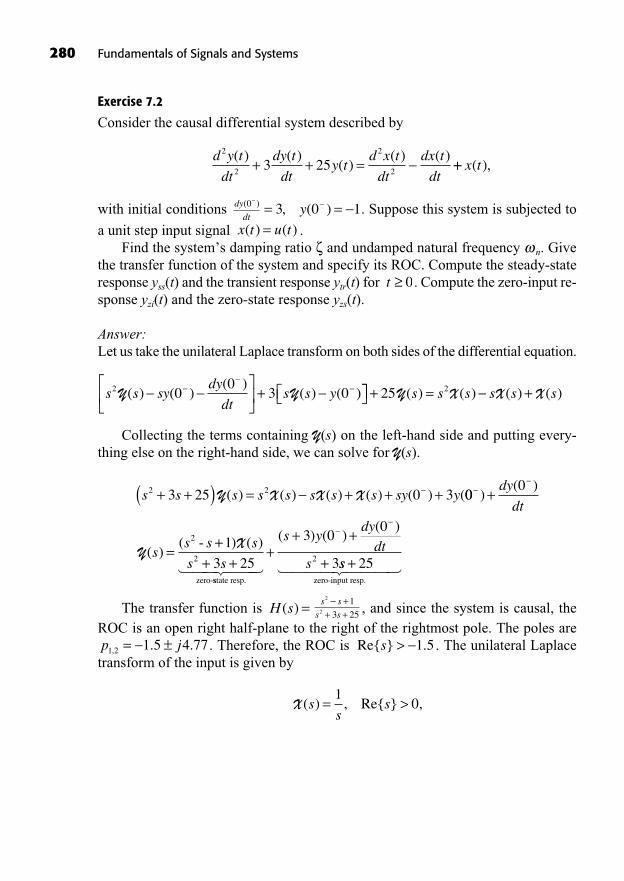
Exercise 7.2
Consider the causal differential system described by
with initial conditions . Suppose this system is subjected to
a unit step input signal .Find the system’s damping ratio and undamped natural frequency n. Give
the transfer function of the system and specify its ROC. Compute the steady-stateresponse yss(t) and the transient response ytr(t) for . Compute the zero-input re-sponse yzi(t) and the zero-state response yzs(t).
Answer:Let us take the unilateral Laplace transform on both sides of the differential equation.
Collecting the terms containing Y(s) on the left-hand side and putting every-thing else on the right-hand side, we can solve for Y(s).
The transfer function is , and since the system is causal, theROC is an open right half-plane to the right of the rightmost pole. The poles are
. Therefore, the ROC is . The unilateral Laplacetransform of the input is given by
X ( ) , Re{ } ,ss
s= >1
0
Re{ } .s > 1 5p j1 2 1 5 4 77, . .= ±
s s
s s
++ +
2
2
1
3 25H s( ) =
s s s s s s s s sy y2 23 25 0 3+ +( ) = + + +Y X X X( ) ( ) ( ) ( ) ( ) (000
1
3 25
2
2
+
=+
+ +
)( )
( )( - ) ( )
dy
dt
ss s s
s sY
X
zero-sstate resp.� ��� ���
++ +
+
( ) ( )( )
s ydydt
s
3 00
32 ss + 25zero-input resp.
� ���� ����
s s sydy
dts s y2 0
03 0Y Y( ) ( )
( )( ) ( )+ + = +25 2Y X X X( ) ( ) ( ) ( )s s s s s s
t 0
x t u t( ) ( )=y, ( )3 0 1= =dy
dt
( )0
d y t
dt
dy t
dty t
d x t
dt
dx t
dt
2
2
2
23 25( ) ( )
( )( ) ( )
+ + = ++ x t( ),
280 Fundamentals of Signals and Systems
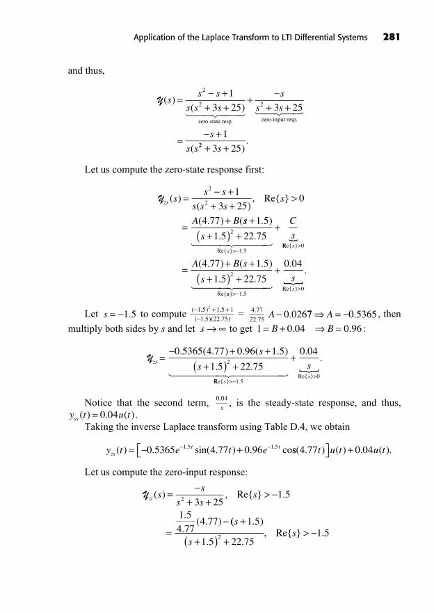
and thus,
Let us compute the zero-state response first:
Let to compute = , then
multiply both sides by s and let to get :
Notice that the second term, , is the steady-state response, and thus,.
Taking the inverse Laplace transform using Table D.4, we obtain
Let us compute the zero-input response:
Yzi ss
s ss( ) , Re{ } .
..
( . )
=+ +
>
=
2 3 251 5
1 54 77
4 77 (( . )
. ., Re{ } .
s
ss
+
+( ) +>
1 5
1 5 22 751 52
y t e t ezst t( ) . sin( . ) . co. .= +0 5365 4 77 0 961 5 1 5 ss( . ) ( ) . ( ).4 77 0 04t u t u t+
y t u tss ( ) . ( )= 0 04
0 04.
s
Yzs
s
s=
+ ++( ) +
0 5365 4 77 0 96 1 5
1 5 22 752
. ( . ) . ( . )
. .RRe{ } .
Re{ }
..
ss
s
>>
+
1 50
0 04
� ������ ������ �
1 0 04 0 96= + =B B. .s
.0 026A 77 0 5365=A ..
.
4 77
22 75
( . ) .
( . )( . )
+ +1 5 1 5 1
1 5 22 75
2
s = 1 5.
Yzs ss s
s s ss
A B
( )( )
, Re{ }
( . ) (
=+
+ +>
=+
2
2
1
3 250
4 77 ss
s
C
s
s
++( ) +
+
>
1 5
1 5 22 752
1 5
. )
. .Re{ } .
� ���� ���� RRe{ }
Re{
( . ) ( . )
. .
s
A B s
s
>
=+ +
+( ) +
0
2
4 77 1 5
1 5 22 75
�
sss
s
} .Re{ }
..
>>
+
1 50
0 04
� ���� ���� �
Y( )( )
ss s
s s s=
++ +
2
2
1
3 25zero-state resp.
� ��� ���� � �� ��+
+ +
=+
s
s s
s
s s
2 3 25
1
zero-input resp.
( 22 3 25+ +s ).
Application of the Laplace Transform to LTI Differential Systems 281
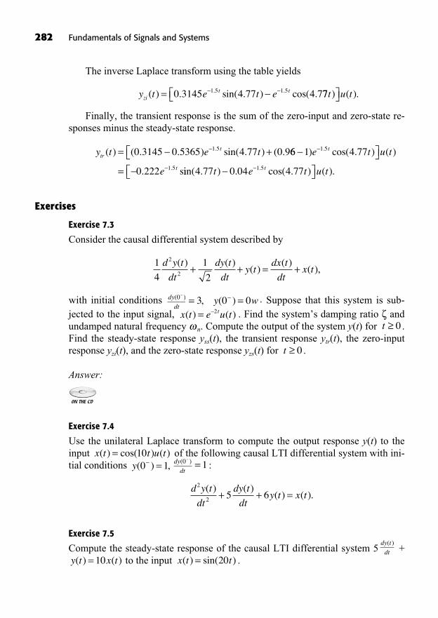
282 Fundamentals of Signals and Systems
The inverse Laplace transform using the table yields
Finally, the transient response is the sum of the zero-input and zero-state re-sponses minus the steady-state response.
Exercises
Exercise 7.3
Consider the causal differential system described by
with initial conditions . Suppose that this system is sub-jected to the input signal, . Find the system’s damping ratio andundamped natural frequency n. Compute the output of the system y(t) for .Find the steady-state response yss(t), the transient response ytr(t), the zero-inputresponse yzi(t), and the zero-state response yzs(t) for .
Answer:
Exercise 7.4
Use the unilateral Laplace transform to compute the output response y(t) to theinput of the following causal LTI differential system with ini-tial conditions :
Exercise 7.5
Compute the steady-state response of the causal LTI differential system 5 +to the input .x t t( ) sin( )= 2010y t x t( ) ( )=
dy t
dt
( )
d y t
dt
dy t
dty t x t
2
2 5 6( ) ( )
( ) ( ).+ + =
1=dy
dt
( )0y( ) ,0 1=x t t u t( ) cos( ) ( )= 10
t 0
t 0x t e u tt( ) ( )= 2
y w, ( )3 0 0= =dy
dt
( )0
1
4
1
2
2
2
d y t
dt
dy t
dty t
dx t
dtx t
( ) ( )( )
( )( ),+ + = +
y t e ttrt( ) ( . . ) sin( . ) ( ..= +0 3145 0 5365 4 77 0 91 5 66 1 4 77
0 222
1 5
1 5=
) cos( . ) ( )
. s
.
.
e t u t
e
t
t iin( . ) . cos( . ) ( )..4 77 0 04 4 771 5t e t u tt
y t e t ezit t( ) . sin( . ) cos( .. .= 0 3145 4 77 4 71 5 1 5 77t u t) ( ).
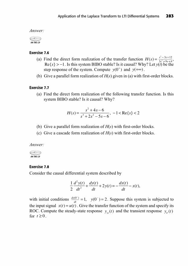
Application of the Laplace Transform to LTI Differential Systems 283
Answer:
Exercise 7.6
(a) Find the direct form realization of the transfer function ,. Is this system BIBO stable? Is it causal? Why? Let y(t) be the
step response of the system. Compute and .
(b) Give a parallel form realization of H(s) given in (a) with first-order blocks.
Exercise 7.7
(a) Find the direct form realization of the following transfer function. Is thissystem BIBO stable? Is it causal? Why?
(b) Give a parallel form realization of H(s) with first-order blocks.
(c) Give a cascade form realization of H(s) with first-order blocks.
Answer:
Exercise 7.8
Consider the causal differential system described by
with initial conditions . Suppose this system is subjected to
the input signal . Give the transfer function of the system and specify itsROC. Compute the steady-state response and the transient response for .t 0
y ttr ( )y tss ( )x t u t( ) ( )=
y, ( )1 0 2= =dy
dt
( )0
1
22
2
2
d y t
dt
dy t
dty t
dx t
dtx t
( ) ( )( )
( )( ),+ + =
H ss s
s s ss( ) , Re{ }=
++
< <2
3 2
4 6
2 5 61 2
y( )+y( )0+sRe{ } > 1
s s
s s
++ +
2
2
3 12
3 9 6H s( ) =

This page intentionally left blank
285
Time and Frequency Analysis of BIBO Stable,Continuous-Time LTI Systems
8
In This Chapter
Relation of Poles and Zeros of the Transfer Function to the Frequency ResponseBode PlotsFrequency Response of First-Order Lag, Lead, and Second-OrderLead-Lag SystemsFrequency Response of Second-Order SystemsStep Response of Stable LTI SystemsIdeal Delay SystemsGroup DelayNon-Minimum Phase and All-Pass SystemsSummaryTo Probe FurtherExercises
((Lecture 26: Qualitative Evaluation of the Frequency Response from the Pole-Zero Plot))
In this chapter, we will analyze the behavior of stable continuous-time lineartime-invariant (LTI) systems by looking at both the time-domain and the fre-quency-domain points of view. We will see how to get a feel for the frequency
response of a system by looking at its transfer function in pole-zero form. We willalso introduce the Bode plot, which is a representation of the frequency responseof a system that can be sketched by hand.
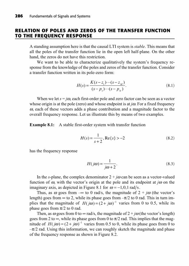
286 Fundamentals of Signals and Systems
RELATION OF POLES AND ZEROS OF THE TRANSFER FUNCTIONTO THE FREQUENCY RESPONSE
A standing assumption here is that the causal LTI system is stable. This means thatall the poles of the transfer function lie in the open left half-plane. On the otherhand, the zeros do not have this restriction.
We want to be able to characterize qualitatively the system’s frequency re-sponse from the knowledge of the poles and zeros of the transfer function. Considera transfer function written in its pole-zero form:
(8.1)
When we let s = j , each first-order pole and zero factor can be seen as a vectorwhose origin is at the pole (zero) and whose endpoint is at j . For a fixed frequency
, each of these vectors adds a phase contribution and a magnitude factor to theoverall frequency response. Let us illustrate this by means of two examples.
Example 8.1: A stable first-order system with transfer function
(8.2)
has the frequency response
(8.3)
In the s-plane, the complex denominator 2 + j can be seen as a vector-valuedfunction of , with the vector’s origin at the pole and its endpoint at j on theimaginary axis, as depicted in Figure 8.1 for .
Thus, as goes from – to 0 rad/s, the magnitude of 2 + j (the vector’slength) goes from to 2, while its phase goes from – /2 to 0 rad. This in turn im-plies that the magnitude of varies from 0 to 0.5, while itsphase goes from /2 to 0 rad.
Then, as goes from 0 to rad/s, the magnitude of 2 + j (the vector’s length)goes from 2 to , while its phase goes from 0 to /2 rad. This implies that the mag-nitude of varies from 0.5 to 0, while its phase goes from 0 to– /2 rad. Using this information, we can roughly sketch the magnitude and phaseof the frequency response as shown in Figure 8.2.
H j j( ) ( )= +2 1
H j j( ) ( )= +2 1
= 1 0 1, , rad s
H jj
( ) .=+
1
2
H ss
s( ) , Re{ }=+
>1
22
H sK s z s z
s p s pM
N
( )( ) ( )
( ) ( ).= 1
1
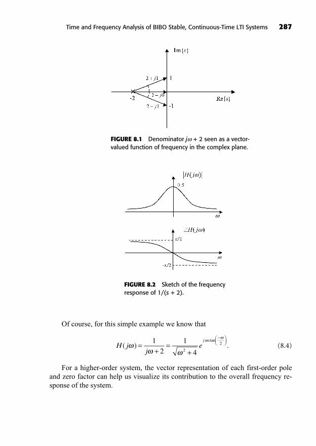
Of course, for this simple example we know that
(8.4)
For a higher-order system, the vector representation of each first-order poleand zero factor can help us visualize its contribution to the overall frequency re-sponse of the system.
H jj
ej
( ) .arctan
=+
=+
1
2
1
42
2
Time and Frequency Analysis of BIBO Stable, Continuous-Time LTI Systems 287
FIGURE 8.1 Denominator j + 2 seen as a vector-valued function of frequency in the complex plane.
FIGURE 8.2 Sketch of the frequencyresponse of 1/(s + 2).
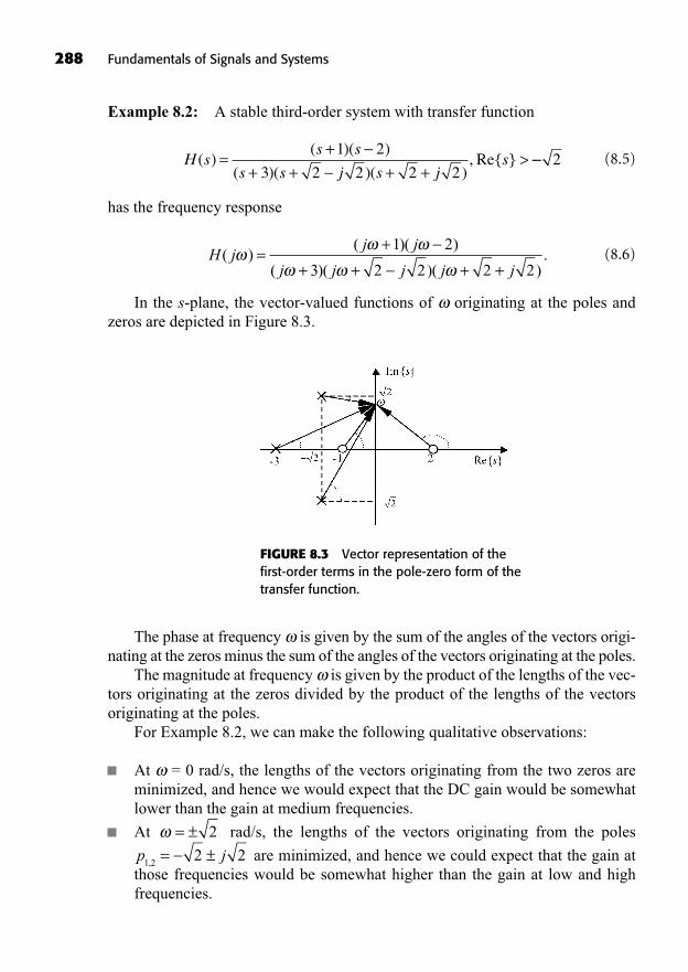
288 Fundamentals of Signals and Systems
Example 8.2: A stable third-order system with transfer function
(8.5)
has the frequency response
(8.6)
In the s-plane, the vector-valued functions of originating at the poles andzeros are depicted in Figure 8.3.
H jj j
j j j j j( )
( )( )
( )( )( ).=
++ + + +
1 2
3 2 2 2 2
H ss s
s s j s js( )
( )( )
( )( )( ), Re{ }=
++ + + +
>1 2
3 2 2 2 22
FIGURE 8.3 Vector representation of thefirst-order terms in the pole-zero form of thetransfer function.
The phase at frequency is given by the sum of the angles of the vectors origi-nating at the zeros minus the sum of the angles of the vectors originating at the poles.
The magnitude at frequency is given by the product of the lengths of the vec-tors originating at the zeros divided by the product of the lengths of the vectorsoriginating at the poles.
For Example 8.2, we can make the following qualitative observations:
At = 0 rad/s, the lengths of the vectors originating from the two zeros areminimized, and hence we would expect that the DC gain would be somewhatlower than the gain at medium frequencies.
At rad/s, the lengths of the vectors originating from the poles
are minimized, and hence we could expect that the gain atthose frequencies would be somewhat higher than the gain at low and highfrequencies.
p j1 2
2 2,= ±= ± 2
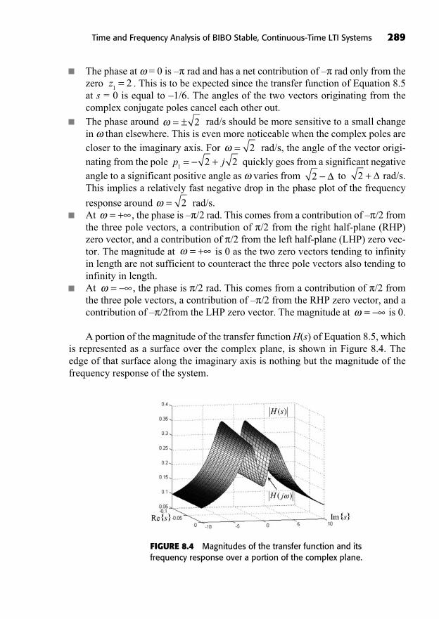
The phase at = 0 is – rad and has a net contribution of – rad only from thezero . This is to be expected since the transfer function of Equation 8.5at s = 0 is equal to –1/6. The angles of the two vectors originating from thecomplex conjugate poles cancel each other out.The phase around rad/s should be more sensitive to a small changein than elsewhere. This is even more noticeable when the complex poles arecloser to the imaginary axis. For rad/s, the angle of the vector origi-nating from the pole quickly goes from a significant negativeangle to a significant positive angle as varies from to rad/s.This implies a relatively fast negative drop in the phase plot of the frequency
response around rad/s.At , the phase is – /2 rad. This comes from a contribution of – /2 fromthe three pole vectors, a contribution of /2 from the right half-plane (RHP)zero vector, and a contribution of /2 from the left half-plane (LHP) zero vec-tor. The magnitude at is 0 as the two zero vectors tending to infinityin length are not sufficient to counteract the three pole vectors also tending toinfinity in length.At , the phase is /2 rad. This comes from a contribution of /2 fromthe three pole vectors, a contribution of – /2 from the RHP zero vector, and acontribution of – /2from the LHP zero vector. The magnitude at is 0.
A portion of the magnitude of the transfer function H(s) of Equation 8.5, whichis represented as a surface over the complex plane, is shown in Figure 8.4. Theedge of that surface along the imaginary axis is nothing but the magnitude of thefrequency response of the system.
=
=
= +
= += 2
2 +2p j
12 2= +
= 2
= ± 2
z1
2=
Time and Frequency Analysis of BIBO Stable, Continuous-Time LTI Systems 289
FIGURE 8.4 Magnitudes of the transfer function and itsfrequency response over a portion of the complex plane.
Remark: The definition of an angle is sometimes ambiguous. In Example 8.2, wehave defined the angle of the right half-plane zero vector as being measured counter-clockwise along positive angles for > 0 and as being measured clockwise along neg-ative angles for < 0. This allowed us to obtain rad,which is consistent with the fact that the frequency-response phase of an LTI differ-ential system with real coefficients is an odd function of frequency. However, for mostpurposes, the angle /2 rad can be considered the same as –3 /2 rad.
((Lecture 27: The Bode Plot))
BODE PLOTS
It is often convenient to use a logarithmic scale to plot the magnitude of a fre-quency response. One reason is that frequency responses can have a wide dynamicrange covering many orders of magnitude. Some frequencies may be amplified bya factor of 1000, while others may be attenuated by a factor of 10–4. Another rea-son is that using a log scale, we can add rather than multiply the magnitudes of cas-caded Fourier transforms, which is easier to do graphically:
(8.7)
It is customary to use the decibel (dB) as the logarithmic unit. The bel (B) wasdefined (after Alexander Graham Bell) as a power amplification of for a system. The decibel is one tenth of a bel. Therefore, for a system with a powergain of 10 at frequency , its power gain in dB is
(8.8)
To measure the actual magnitude gain (not the power gain) of a system, we usethe identity
(8.9)
Thus, a magnitude plot of is represented as usinga linear scale in dB. Table 8.1 shows the correspondence between some gains andtheir values expressed in dB.
20 10log ( )H j dBH j( )
10 2010
2
10log ( ) log ( )H j H jdB dB.=
10 10 10 1010
2
10
dB
BB dB dB.× = =log ( ) logH j
H j( )2
10=
log ( ) log ( ) log ( ) .Y j H j X j= +
= =H j H j( ) ( ) 2
290 Fundamentals of Signals and Systems
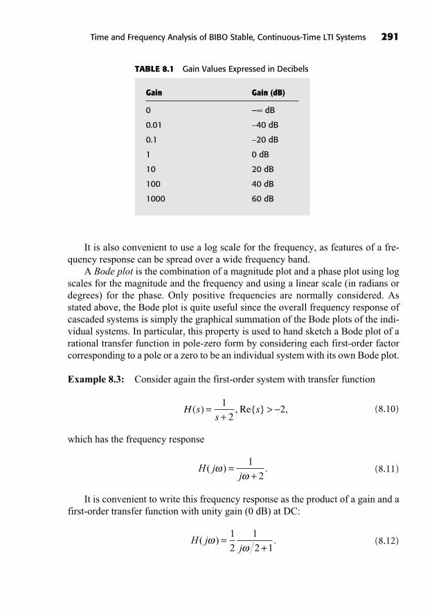
Time and Frequency Analysis of BIBO Stable, Continuous-Time LTI Systems 291
It is also convenient to use a log scale for the frequency, as features of a fre-quency response can be spread over a wide frequency band.
A Bode plot is the combination of a magnitude plot and a phase plot using logscales for the magnitude and the frequency and using a linear scale (in radians ordegrees) for the phase. Only positive frequencies are normally considered. Asstated above, the Bode plot is quite useful since the overall frequency response ofcascaded systems is simply the graphical summation of the Bode plots of the indi-vidual systems. In particular, this property is used to hand sketch a Bode plot of arational transfer function in pole-zero form by considering each first-order factorcorresponding to a pole or a zero to be an individual system with its own Bode plot.
Example 8.3: Consider again the first-order system with transfer function
(8.10)
which has the frequency response
(8.11)
It is convenient to write this frequency response as the product of a gain and afirst-order transfer function with unity gain (0 dB) at DC:
(8.12)H jj
( ) .=+
1
2
1
2 1
H jj
( ) .=+
1
2
H ss
s( ) , Re{ } ,=+
>1
22
Gain Gain (dB)
0 – dB
0.01 40 dB
0.1 20 dB
1 0 dB
10 20 dB
100 40 dB
1000 60 dB
TABLE 8.1 Gain Values Expressed in Decibels

292 Fundamentals of Signals and Systems
The break frequency is 2 rad/s. The Bode magnitude plot is the graph of:
(8.13)
Note that for low frequencies, that is, << 2,
(8.14)
and for high frequencies, that is, ,
(8.15)
For = 10 rad/s in Equation 8.15, we get –20 dB, for = 100 rad/s, we get–40 dB, etc. The slope of the asymptote is therefore –20 decibelsper decade of frequency (a decade is an increase by a factor of 10.) With the as-ymptotes meeting at the break frequency 2 rad/s, we can sketch the magnitudeBode plot as shown in Figure 8.5 (dotted line: actual magnitude.)
20 10log dB
20 6 202
6 20
10 10
10
log ( ) log
log
H j
=
dB dB
dB ddB dB
dB.
+=
20 2
2010
10
log
log
>> 2
20 6 20 1 610 10log ( ) logH j =dB dB dB,
20 201
220
1
1
20
10 10 102
log ( ) log log
l
H j j= ++
=
dB
oog log
log
10 10 2
10 2
2 20 1
6 20 1
+
= +
j
j
dB
dB dB.
FIGURE 8.5 Bode magnitude plot of a first-ordertransfer function.

Time and Frequency Analysis of BIBO Stable, Continuous-Time LTI Systems 293
FIGURE 8.6 Bode phase plot of a first-order transfer function.
The Bode phase plot is the graph of
(8.16)
We know that the phase is 0 at = 0 and at . A piecewise linear ap-proximation (with a log frequency scale) to the phase that helps us sketch it is givenby
(8.17)
The approximation given by Equation 8.17 deserves some explanations. Thephase approximation is constructed as follows:
At frequencies lower than one decade below the break frequency, the phase is 0.At frequencies higher than one decade above the break frequency, the phase is– /2.In the interval from one decade below to one decade above the break fre-quency, the phase is linear and goes from 0 to – /2 with a slope – /4 radian perdecade.
The Bode phase plot is shown in Figure 8.6. The interactive Bode applet on thecompanion CD-ROM located in D:\Applets\BodePlot\Bode.exe lets the user enterpoles and zeros of a transfer function on a pole-zero plot and it then produces aBode plot of the transfer function. Both the actual frequency response plot and thebroken line approximation obtained using the above rules are shown on the applet’sBode plot for comparison.
+[ ] <H j( )
,
log ( )
,
,
0
41
220
210
10 22
10 < 20.
=
=+
=+
=H jj j
( ) arctan .1
2
1
2 1
1
2 1 12
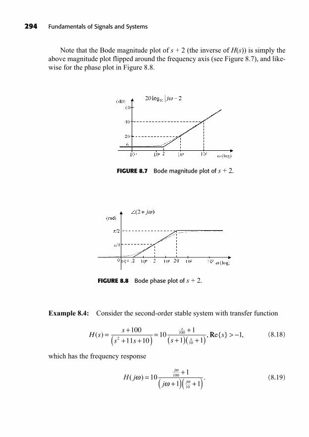
294 Fundamentals of Signals and Systems
Note that the Bode magnitude plot of s + 2 (the inverse of H(s)) is simply theabove magnitude plot flipped around the frequency axis (see Figure 8.7), and like-wise for the phase plot in Figure 8.8.
FIGURE 8.7 Bode magnitude plot of s + 2.
FIGURE 8.8 Bode phase plot of s + 2.
Example 8.4: Consider the second-order stable system with transfer function
(8.18)
which has the frequency response
(8.19)H jj
j
j( ) .=
++( ) +( )10
1
1 1100
10
H ss
s s s
s
s( ) ,=
++ +( ) =
++( ) +( )
100
11 1010
1
1 12100
10
RRe{ } ,s > 1

The break frequencies are at 1, 10, and 100 rad/s. For the Bode magnitude plot,we can sketch the asymptotes of each first-order term in Equation 8.19 on the samemagnitude graph (as dashed lines) and then add them together as shown in Figure 8.9.
Time and Frequency Analysis of BIBO Stable, Continuous-Time LTI Systems 295
FIGURE 8.9 Bode magnitude plot of a second-order example.
We proceed in a similar fashion to obtain the Bode phase plot of Figure 8.10.
FIGURE 8.10 Bode phase plot of a second-order example.
A Bode plot can easily be obtained in MATLAB. The following MATLABscript bodeplot.m, which is located on the CD-ROM in D:\Chapter8, produces theBode plot of Example 8.4.
%% bodeplot.m Bode plot of a transfer function
% transfer function numerator and denominator
num=[1 100];
den=[1 11 10];
sys=tf(num,den);
% frequency vector
w=logspace(-2,4,200);
% Bode plot
bode(sys,w)
((Lecture 28: Frequency Responses of Lead, Lag, and Lead-Lag Systems))
FREQUENCY RESPONSE OF FIRST-ORDER LAG, LEAD, ANDSECOND-ORDER LEAD-LAG SYSTEMS
First-order lag systems and lead systems can be considered as building blocks infilter and controller design. They have simple transfer functions with lowpass andhighpass frequency responses, respectively, which can be combined into a second-order lead-lag system that has applications in sound equalization and feedbackcontrol design.
First-Order Lag
A first-order lag has a transfer function of the form
(8.20)
where , is the time constant and (the absolute value of the pole)is called either the natural frequency, the cutoff frequency, or the break frequency,depending on the application. This system is called a lag because it has an effectsimilar to a pure delay of seconds at low frequencies, especially for = 0.To see this, expand H(s) as a Taylor series around s = 0:
(8.21)
(8.22)e ss ss = + +12 3
2 3( ) ( )
!.…
1
11 2 3
ss s s
+= + +( ) ( ) …
e s
1> 00 1<
H ss
ss( ) , Re{ } ,=
++
>1
1
1
296 Fundamentals of Signals and Systems
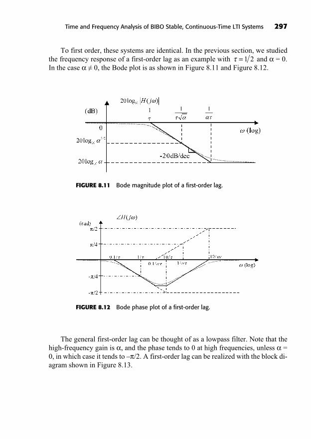
Time and Frequency Analysis of BIBO Stable, Continuous-Time LTI Systems 297
To first order, these systems are identical. In the previous section, we studiedthe frequency response of a first-order lag as an example with and = 0.In the case ≠ 0, the Bode plot is as shown in Figure 8.11 and Figure 8.12.
= 1 2
FIGURE 8.11 Bode magnitude plot of a first-order lag.
FIGURE 8.12 Bode phase plot of a first-order lag.
The general first-order lag can be thought of as a lowpass filter. Note that thehigh-frequency gain is , and the phase tends to 0 at high frequencies, unless =0, in which case it tends to – /2. A first-order lag can be realized with the block di-agram shown in Figure 8.13.
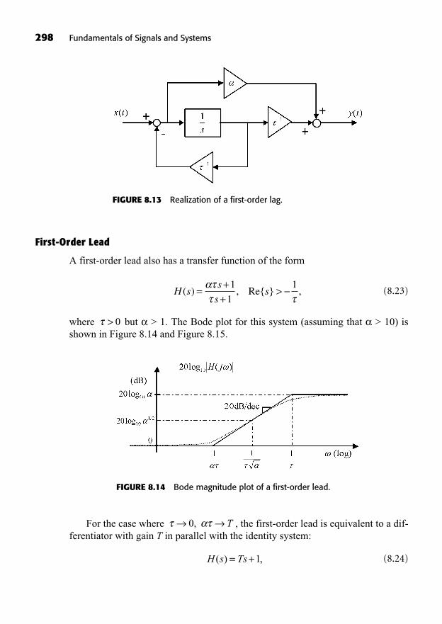
298 Fundamentals of Signals and Systems
FIGURE 8.13 Realization of a first-order lag.
First-Order Lead
A first-order lead also has a transfer function of the form
(8.23)
where but > 1. The Bode plot for this system (assuming that > 10) isshown in Figure 8.14 and Figure 8.15.
> 0
H ss
ss( ) , Re{ } ,=
++
>1
1
1
FIGURE 8.14 Bode magnitude plot of a first-order lead.
For the case where , the first-order lead is equivalent to a dif-ferentiator with gain T in parallel with the identity system:
(8.24)H s Ts( ) ,= +1
0, T

and its Bode plot is given in Figure 8.16. Note that the high frequencies are ampli-fied: the higher the frequency, the higher the gain of the system is. This is a prop-erty of differentiators, and it explains why high-frequency noise is greatlyamplified by such devices. The maximum positive phase is /2 rad for .= +
Time and Frequency Analysis of BIBO Stable, Continuous-Time LTI Systems 299
FIGURE 8.15 Bode phase plot of a first-order lead.
FIGURE 8.16 Bode plot of a limit case of first-order lead H(s) = Ts + 1.
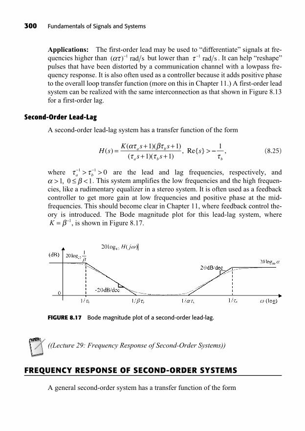
300 Fundamentals of Signals and Systems
Applications: The first-order lead may be used to “differentiate” signals at fre-quencies higher than but lower than . It can help “reshape”pulses that have been distorted by a communication channel with a lowpass fre-quency response. It is also often used as a controller because it adds positive phaseto the overall loop transfer function (more on this in Chapter 11.) A first-order leadsystem can be realized with the same interconnection as that shown in Figure 8.13for a first-order lag.
Second-Order Lead-Lag
A second-order lead-lag system has a transfer function of the form
(8.25)
where are the lead and lag frequencies, respectively, and. This system amplifies the low frequencies and the high frequen-
cies, like a rudimentary equalizer in a stereo system. It is often used as a feedbackcontroller to get more gain at low frequencies and positive phase at the mid-frequencies. This should become clear in Chapter 11, where feedback control the-ory is introduced. The Bode magnitude plot for this lead-lag system, where
, is shown in Figure 8.17.K = 1
> <1 0 1,a b> >1 1 0
H sK s s
s ssa b
a b
( )( )( )
( )( ), Re{ }=
+ ++ +
>1 1
1 1
1
b
,
1 rad s( ) 1 rad s
FIGURE 8.17 Bode magnitude plot of a second-order lead-lag.
((Lecture 29: Frequency Response of Second-Order Systems))
FREQUENCY RESPONSE OF SECOND-ORDER SYSTEMS
A general second-order system has a transfer function of the form
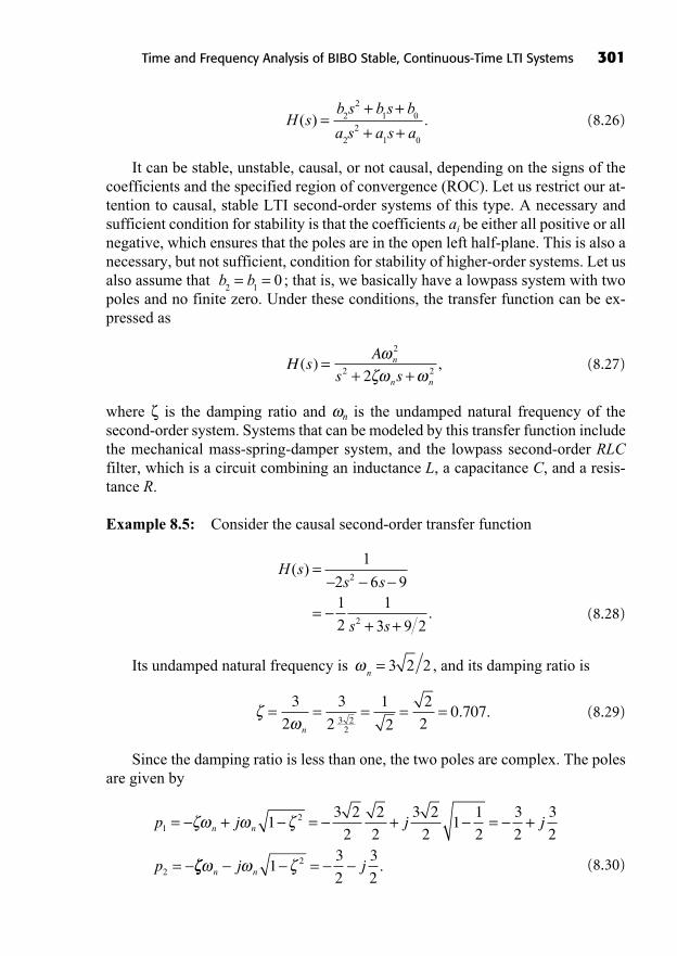
(8.26)
It can be stable, unstable, causal, or not causal, depending on the signs of thecoefficients and the specified region of convergence (ROC). Let us restrict our at-tention to causal, stable LTI second-order systems of this type. A necessary andsufficient condition for stability is that the coefficients ai be either all positive or allnegative, which ensures that the poles are in the open left half-plane. This is also anecessary, but not sufficient, condition for stability of higher-order systems. Let usalso assume that ; that is, we basically have a lowpass system with twopoles and no finite zero. Under these conditions, the transfer function can be ex-pressed as
(8.27)
where is the damping ratio and n is the undamped natural frequency of the second-order system. Systems that can be modeled by this transfer function includethe mechanical mass-spring-damper system, and the lowpass second-order RLCfilter, which is a circuit combining an inductance L, a capacitance C, and a resis-tance R.
Example 8.5: Consider the causal second-order transfer function
(8.28)
Its undamped natural frequency is , and its damping ratio is
(8.29)
Since the damping ratio is less than one, the two poles are complex. The polesare given by
(8.30)
p j j j
p
n n12
2
13 2
2
2
2
3 2
21
1
2
3
2
3
2= + = + = +
= n nj j=13
2
3
22 .
= = = = =3
2
3
2
1
2
2
20 707
3 22n
. .
n= 3 2 2
H ss s
s s
( )
.
=
=+ +
1
2 6 91
2
1
3 9 2
2
2
H sA
s sn
n n
( ) ,=+ +
2
2 22
b b2 1
0= =
H sb s b s b
a s a s a( ) .=
+ ++ +
22
1 0
22
1 0
Time and Frequency Analysis of BIBO Stable, Continuous-Time LTI Systems 301
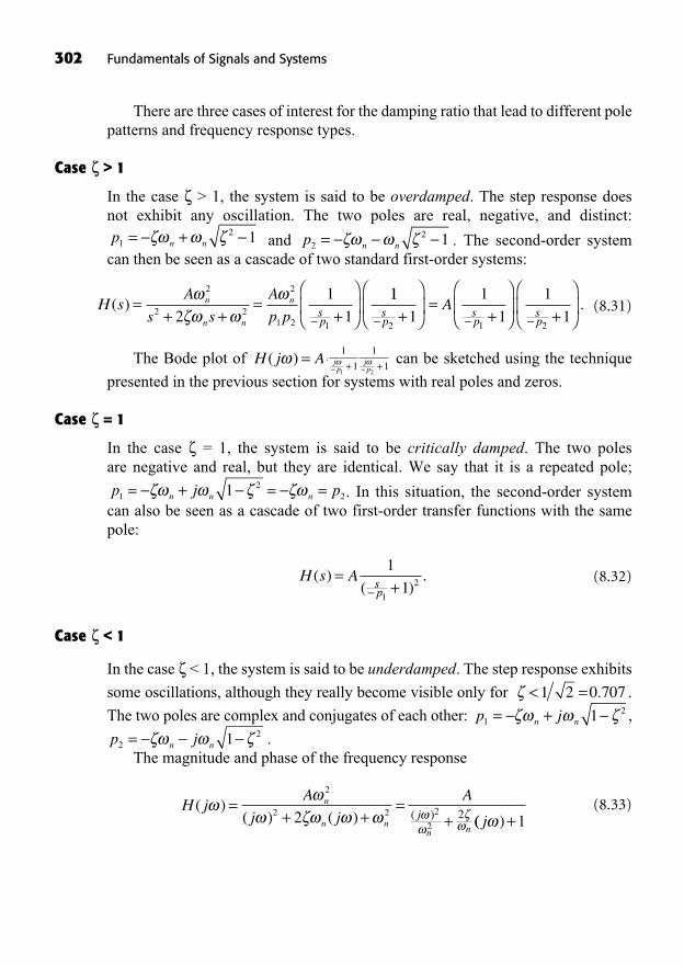
There are three cases of interest for the damping ratio that lead to different polepatterns and frequency response types.
Case > 1
In the case > 1, the system is said to be overdamped. The step response does not exhibit any oscillation. The two poles are real, negative, and distinct:
and . The second-order systemcan then be seen as a cascade of two standard first-order systems:
(8.31)
The Bode plot of can be sketched using the technique
presented in the previous section for systems with real poles and zeros.
Case = 1
In the case = 1, the system is said to be critically damped. The two poles are negative and real, but they are identical. We say that it is a repeated pole;
. In this situation, the second-order systemcan also be seen as a cascade of two first-order transfer functions with the samepole:
(8.32)
Case < 1
In the case < 1, the system is said to be underdamped. The step response exhibits
some oscillations, although they really become visible only for .
The two poles are complex and conjugates of each other: ,
.The magnitude and phase of the frequency response
(8.33)H jA
j j
An
n nj
n n
( )( ) ( ) ( )
=+ +
=+
2
2 22 2
22 (( )j +1
p jn n221=
p jn n121= +
< =1 2 0 707.
H s Asp
( )( )
.=+1
11
2
p j pn n n12
21= + = =
A jp
jp+ +
1
1
1
11 2
H j A( ) =
H sA
s s
A
p pn
n n
n
sp
( ) =+ +
=+
2
2 2
2
1 22
1
11
11
1
1
1
1
12 1 2sp
sp
sp
A+
=+ +
.
p n n22 1=p n n1
2 1= +
302 Fundamentals of Signals and Systems
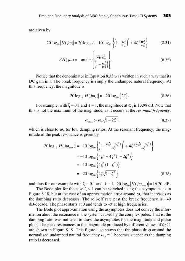
are given by
(8.34)
(8.35)
Notice that the denominator in Equation 8.33 was written in such a way that itsDC gain is 1. The break frequency is simply the undamped natural frequency. Atthis frequency, the magnitude is
(8.36)
For example, with = 0.1 and A = 1, the magnitude at n is 13.98 dB. Note thatthis is not the maximum of the magnitude, as it occurs at the resonant frequency,
(8.37)
which is close to n for low damping ratios. At the resonant frequency, the mag-nitude of the peak resonance is given by
(8.38)
and thus for our example with = 0.1 and A = 1, .The Bode plot for the case < 1 can be sketched using the asymptotes as in
Figure 8.18, but at the cost of an approximation error around n that increases asthe damping ratio decreases. The roll-off rate past the break frequency is 40dB/decade. The phase starts at 0 and tends to – at high frequencies.
The Bode plot approximation using the asymptotes does not convey the infor-mation about the resonance in the system caused by the complex poles. That is, thedamping ratio was not used to draw the asymptotes for the magnitude and phaseplots. The peak resonances in the magnitude produced by different values of ≤ 1are shown in Figure 8.19. This figure also shows that the phase drop around thenormalized undamped natural frequency n = 1 becomes steeper as the dampingratio is decreased.
20 16 2010log ( ) .maxH j = dB
20 10 110 10
22 2
21 2log ( ) logmax
( )H j n
n= ( ) + 44
10 4 4 1 2
2
104 2
2 2
21 2n
n
( )
log (= + 2
102 2
102
10 4 1
20 2 1
)
log ( )
log
{ }= { }= { }
max : ,= n 1 2 2
20 20 210 10log ( ) log .H j n = { }
= ( )H j n
n
( ) arctan .2
122
20 20 10 1 410 10 10
222
2log ( ) log logH j An
= ( ) + 22n
Time and Frequency Analysis of BIBO Stable, Continuous-Time LTI Systems 303
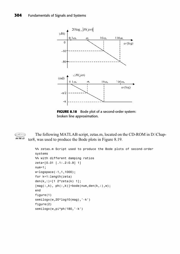
304 Fundamentals of Signals and Systems
FIGURE 8.18 Bode plot of a second-order system:broken line approximation.
The following MATLAB script, zetas.m, located on the CD-ROM in D:\Chap-ter8, was used to produce the Bode plots in Figure 8.19.
%% zetas.m Script used to produce the Bode plots of second-order
systems
%% with different damping ratios
zeta=[0.01 [.1:.2:0.9] 1]
num=1;
w=logspace(-1,1,1000);
for k=1:length(zeta)
den(k,:)=[1 2*zeta(k) 1];
[mag(:,k), ph(:,k)]=bode(num,den(k,:),w);
end
figure(1)
semilogx(w,20*log10(mag),’-k’)
figure(2)
semilogx(w,pi*ph/180,’-k’)
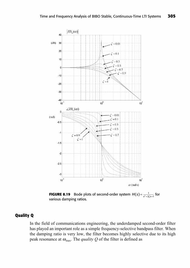
Quality Q
In the field of communications engineering, the underdamped second-order filterhas played an important role as a simple frequency-selective bandpass filter. Whenthe damping ratio is very low, the filter becomes highly selective due to its highpeak resonance at max. The quality Q of the filter is defined as
Time and Frequency Analysis of BIBO Stable, Continuous-Time LTI Systems 305
FIGURE 8.19 Bode plots of second-order system forvarious damping ratios.
s s+ +12 12H s( )=
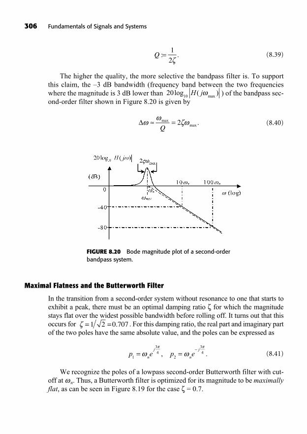
306 Fundamentals of Signals and Systems
(8.39)
The higher the quality, the more selective the bandpass filter is. To support this claim, the –3 dB bandwidth (frequency band between the two frequencieswhere the magnitude is 3 dB lower than ) of the bandpass sec-ond-order filter shown in Figure 8.20 is given by
(8.40)=maxmax .
Q2
2010
log ( )max
H j
Q : .=1
2
FIGURE 8.20 Bode magnitude plot of a second-orderbandpass system.
Maximal Flatness and the Butterworth Filter
In the transition from a second-order system without resonance to one that starts toexhibit a peak, there must be an optimal damping ratio for which the magnitudestays flat over the widest possible bandwidth before rolling off. It turns out that thisoccurs for . For this damping ratio, the real part and imaginary partof the two poles have the same absolute value, and the poles can be expressed as
(8.41)
We recognize the poles of a lowpass second-order Butterworth filter with cut-off at n. Thus, a Butterworth filter is optimized for its magnitude to be maximallyflat, as can be seen in Figure 8.19 for the case = 0.7.
p e p en
j
n
j
1
34
2
34= =, .
= =1 2 0 707.
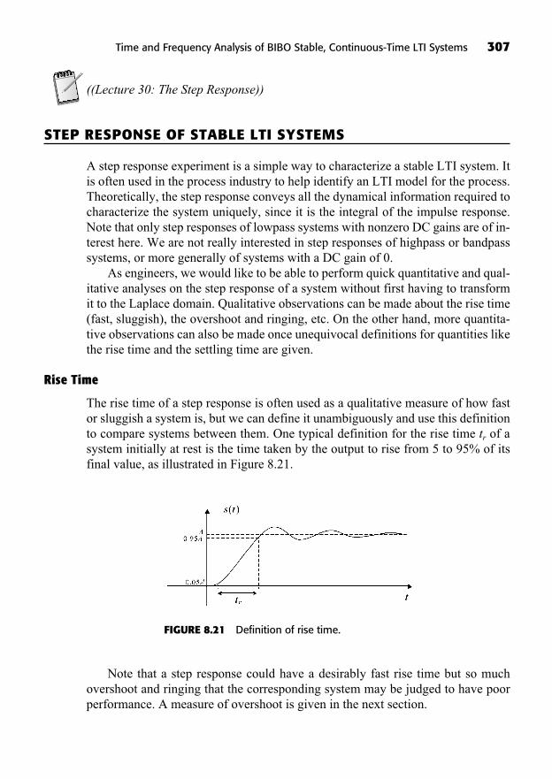
((Lecture 30: The Step Response))
STEP RESPONSE OF STABLE LTI SYSTEMS
A step response experiment is a simple way to characterize a stable LTI system. Itis often used in the process industry to help identify an LTI model for the process.Theoretically, the step response conveys all the dynamical information required tocharacterize the system uniquely, since it is the integral of the impulse response.Note that only step responses of lowpass systems with nonzero DC gains are of in-terest here. We are not really interested in step responses of highpass or bandpasssystems, or more generally of systems with a DC gain of 0.
As engineers, we would like to be able to perform quick quantitative and qual-itative analyses on the step response of a system without first having to transformit to the Laplace domain. Qualitative observations can be made about the rise time(fast, sluggish), the overshoot and ringing, etc. On the other hand, more quantita-tive observations can also be made once unequivocal definitions for quantities likethe rise time and the settling time are given.
Rise Time
The rise time of a step response is often used as a qualitative measure of how fastor sluggish a system is, but we can define it unambiguously and use this definitionto compare systems between them. One typical definition for the rise time tr of asystem initially at rest is the time taken by the output to rise from 5 to 95% of itsfinal value, as illustrated in Figure 8.21.
Time and Frequency Analysis of BIBO Stable, Continuous-Time LTI Systems 307
FIGURE 8.21 Definition of rise time.
Note that a step response could have a desirably fast rise time but so muchovershoot and ringing that the corresponding system may be judged to have poorperformance. A measure of overshoot is given in the next section.
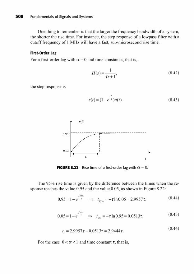
308 Fundamentals of Signals and Systems
One thing to remember is that the larger the frequency bandwidth of a system,the shorter the rise time. For instance, the step response of a lowpass filter with acutoff frequency of 1 MHz will have a fast, sub-microsecond rise time.
First-Order Lag
For a first-order lag with = 0 and time constant , that is,
(8.42)
the step response is
(8.43)s t e u tt
( ) ( ) ( ).= 1
H ss
( ) ,=+1
1
FIGURE 8.22 Rise time of a first-order lag with = 0.
The 95% rise time is given by the difference between the times when the re-sponse reaches the value 0.95 and the value 0.05, as shown in Figure 8.22:
(8.44)
(8.45)
(8.46)
For the case and time constant , that is,0 1< <
tr= =2 9957 0 0513 2 9444. . . .
0 05 1 0 95 0 05135
5. ln . . .
%
%= = =e t
t
0 95 1 0 05 2 995795
95. ln . . .
%
%= = =e t
t
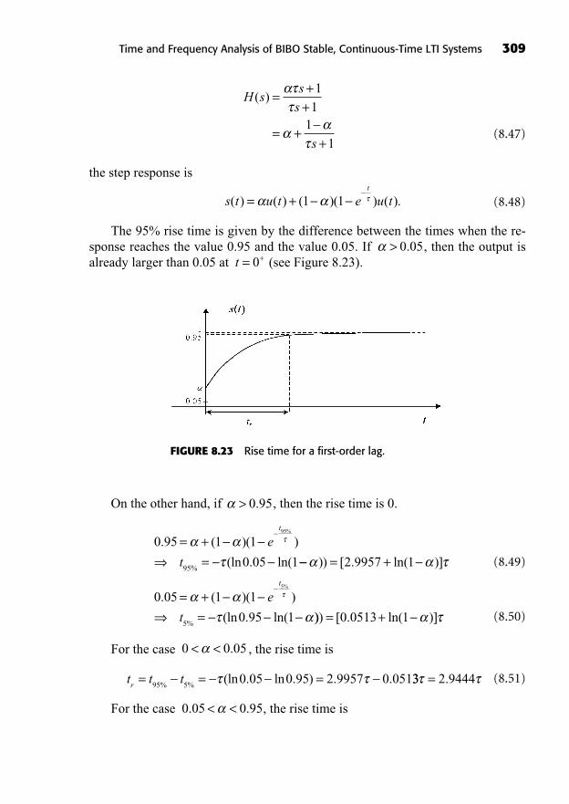
(8.47)
the step response is
(8.48)
The 95% rise time is given by the difference between the times when the re-sponse reaches the value 0.95 and the value 0.05. If , then the output isalready larger than 0.05 at (see Figure 8.23).t = +0
> 0 05.
s t u t e u tt
( ) ( ) ( )( ) ( ).= + 1 1
H ss
s
s
( ) =++
= ++
1
11
1
Time and Frequency Analysis of BIBO Stable, Continuous-Time LTI Systems 309
FIGURE 8.23 Rise time for a first-order lag.
On the other hand, if , then the rise time is 0.
(8.49)
(8.50)
For the case , the rise time is
(8.51)
For the case , the rise time is0 05 0 95. .< <
t t tr= = =
95 50 05 0 95 2 9957 0 051
% %(ln . ln . ) . . 33 2 9444= .
0 0 05< < .
0 05 1 1
0 95 1
5
5
. ( )( )
(ln . ln(
%
%
= +=
e
t
t
))) [ . ln( )]= +0 0513 1
0 95 1 1
0 05 1
95
95
. ( )( )
(ln . ln(
%
%
= +=
e
t
t
= +)) [ . ln( )]2 9957 1
> 0 95.
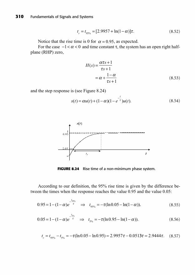
310 Fundamentals of Signals and Systems
(8.52)
Notice that the rise time is 0 for , as expected.For the case and time constant , the system has an open right half-
plane (RHP) zero,
(8.53)
and the step response is (see Figure 8.24)
(8.54)s t u t e u tt
( ) ( ) ( )( ) ( ).= + 1 1
H ss
s
s
( ) =++
= ++
1
11
1
< <1 0= 0 95.
t tr= = +
952 9957 1
%[ . ln( )] .
FIGURE 8.24 Rise time of a non-minimum phase system.
According to our definition, the 95% rise time is given by the difference be-tween the times when the response reaches the value 0.95 and the value 0.05:
(8.55)
(8.56)
(8.57)t t tr= = =
95 50 05 0 95 2 9957 0 051
% %(ln . ln . ) . . 33 2 9444= . .
0 05 1 1 0 95 15
5. ( ) (ln . ln( )).
%
%= =e t
t
0 95 1 1 0 05 195
95. ( ) (ln . ln( ))
%
%= =e t
t
..
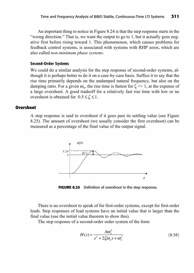
An important thing to notice in Figure 8.24 is that the step response starts in the“wrong direction.” That is, we want the output to go to 1, but it actually goes neg-ative first before rising toward 1. This phenomenon, which causes problems forfeedback control systems, is associated with systems with RHP zeros, which arealso called non-minimum phase systems.
Second-Order Systems
We could do a similar analysis for the step response of second-order systems, al-though it is perhaps better to do it on a case-by-case basis. Suffice it to say that therise time primarily depends on the undamped natural frequency, but also on thedamping ratio. For a given n, the rise time is fastest for << 1, at the expense ofa large overshoot. A good tradeoff for a relatively fast rise time with low or noovershoot is obtained for .
Overshoot
A step response is said to overshoot if it goes past its settling value (see Figure8.25). The amount of overshoot (we usually consider the first overshoot) can bemeasured as a percentage of the final value of the output signal.
0 5 1.
Time and Frequency Analysis of BIBO Stable, Continuous-Time LTI Systems 311
FIGURE 8.25 Definition of overshoot in the step response.
There is no overshoot to speak of for first-order systems, except for first-orderleads. Step responses of lead systems have an initial value that is larger than thefinal value (use the initial value theorem to show this).
The step response of a second-order order system of the form
(8.58)H sA
s sn
n n
( ) =+ +
2
2 22
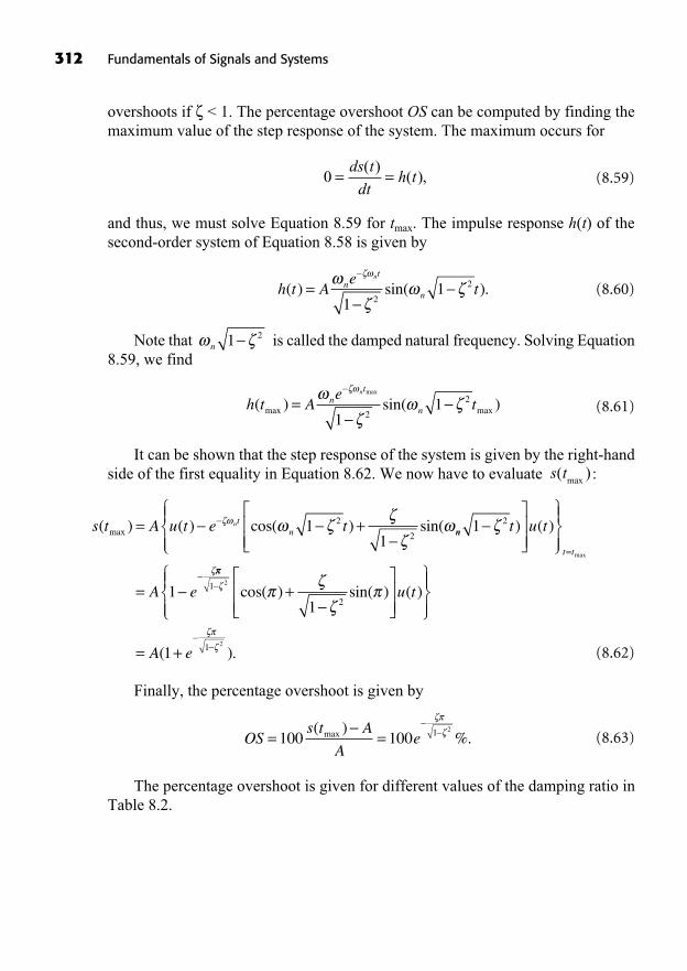
overshoots if < 1. The percentage overshoot OS can be computed by finding themaximum value of the step response of the system. The maximum occurs for
(8.59)
and thus, we must solve Equation 8.59 for tmax. The impulse response h(t) of thesecond-order system of Equation 8.58 is given by
(8.60)
Note that is called the damped natural frequency. Solving Equation8.59, we find
(8.61)
It can be shown that the step response of the system is given by the right-handside of the first equality in Equation 8.62. We now have to evaluate :
(8.62)
Finally, the percentage overshoot is given by
(8.63)
The percentage overshoot is given for different values of the damping ratio inTable 8.2.
OSs t A
Ae= =100 100 1 2( )
%.max
s t A u t e tntn( ) ( ) cos( ) sin(max = +1
1
2
2 nn
t t
t u t
A e
1
1
2
=
=
) ( )
max
1
2
2
1+cos( ) sin( ) ( )u t
= +A e( ).1 1 2
s t( )max
h t Ae
tnt
n
n
( ) sin( )max max
max
=1
12
2
n 1 2
h t Ae
tnt
n
n
( ) sin( ).=1
12
2
0 = =ds t
dth t
( )( ),
312 Fundamentals of Signals and Systems
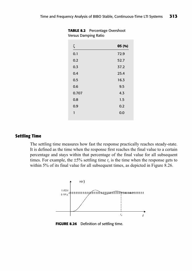
Settling Time
The settling time measures how fast the response practically reaches steady-state.It is defined as the time when the response first reaches the final value to a certainpercentage and stays within that percentage of the final value for all subsequenttimes. For example, the ±5% settling time ts is the time when the response gets towithin 5% of its final value for all subsequent times, as depicted in Figure 8.26.
Time and Frequency Analysis of BIBO Stable, Continuous-Time LTI Systems 313
OS (%)
0.1 72.9
0.2 52.7
0.3 37.2
0.4 25.4
0.5 16.3
0.6 9.5
0.707 4.3
0.8 1.5
0.9 0.2
1 0.0
TABLE 8.2 Percentage OvershootVersus Damping Ratio
FIGURE 8.26 Definition of settling time.
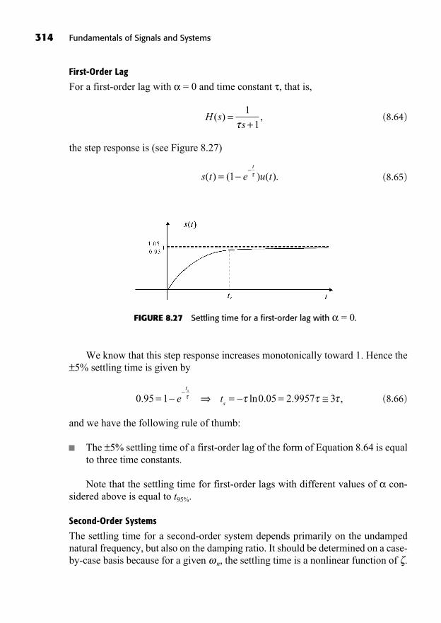
314 Fundamentals of Signals and Systems
First-Order Lag
For a first-order lag with = 0 and time constant , that is,
(8.64)
the step response is (see Figure 8.27)
(8.65)s t e u tt
( ) ( ) ( ).= 1
H ss
( ) ,=+1
1
FIGURE 8.27 Settling time for a first-order lag with = 0.
We know that this step response increases monotonically toward 1. Hence the±5% settling time is given by
(8.66)
and we have the following rule of thumb:
The ±5% settling time of a first-order lag of the form of Equation 8.64 is equalto three time constants.
Note that the settling time for first-order lags with different values of con-sidered above is equal to t95%.
Second-Order Systems
The settling time for a second-order system depends primarily on the undampednatural frequency, but also on the damping ratio. It should be determined on a case-by-case basis because for a given n, the settling time is a nonlinear function of .
0 95 1 0 05 2 9957 3. ln . . ,= = =e tt
s
s
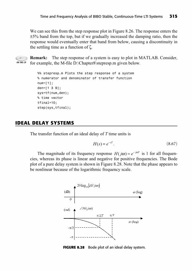
We can see this from the step response plot in Figure 8.26. The response enters the±5% band from the top, but if we gradually increased the damping ratio, then theresponse would eventually enter that band from below, causing a discontinuity inthe settling time as a function of .
Remark: The step response of a system is easy to plot in MATLAB. Consider,for example, the M-file D:\Chapter8\stepresp.m given below.
%% stepresp.m Plots the step response of a system
% numerator and denominator of transfer function
num=[1];
den=[1 3 9];
sys=tf(num,den);
% time vector
tfinal=10;
step(sys,tfinal);
IDEAL DELAY SYSTEMS
The transfer function of an ideal delay of T time units is
(8.67)
The magnitude of its frequency response is 1 for all frequen-cies, whereas its phase is linear and negative for positive frequencies. The Bodeplot of a pure delay system is shown in Figure 8.28. Note that the phase appears tobe nonlinear because of the logarithmic frequency scale.
H j e j T( ) =
H s e sT( ) .=
Time and Frequency Analysis of BIBO Stable, Continuous-Time LTI Systems 315
FIGURE 8.28 Bode plot of an ideal delay system.
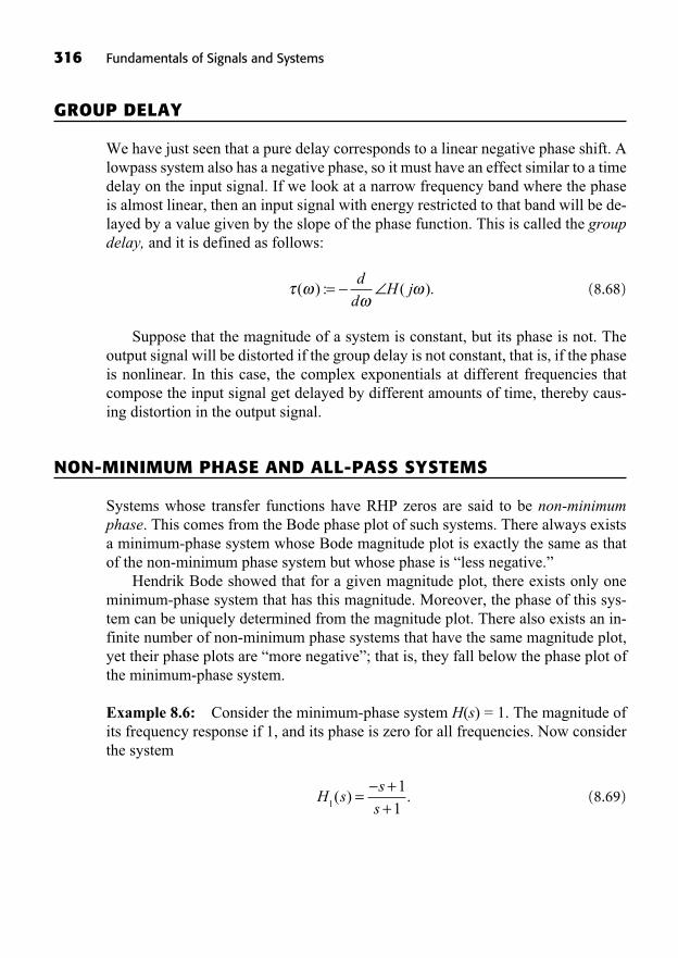
GROUP DELAY
We have just seen that a pure delay corresponds to a linear negative phase shift. Alowpass system also has a negative phase, so it must have an effect similar to a timedelay on the input signal. If we look at a narrow frequency band where the phaseis almost linear, then an input signal with energy restricted to that band will be de-layed by a value given by the slope of the phase function. This is called the groupdelay, and it is defined as follows:
(8.68)
Suppose that the magnitude of a system is constant, but its phase is not. Theoutput signal will be distorted if the group delay is not constant, that is, if the phaseis nonlinear. In this case, the complex exponentials at different frequencies thatcompose the input signal get delayed by different amounts of time, thereby caus-ing distortion in the output signal.
NON-MINIMUM PHASE AND ALL-PASS SYSTEMS
Systems whose transfer functions have RHP zeros are said to be non-minimumphase. This comes from the Bode phase plot of such systems. There always existsa minimum-phase system whose Bode magnitude plot is exactly the same as thatof the non-minimum phase system but whose phase is “less negative.”
Hendrik Bode showed that for a given magnitude plot, there exists only oneminimum-phase system that has this magnitude. Moreover, the phase of this sys-tem can be uniquely determined from the magnitude plot. There also exists an in-finite number of non-minimum phase systems that have the same magnitude plot,yet their phase plots are “more negative”; that is, they fall below the phase plot ofthe minimum-phase system.
Example 8.6: Consider the minimum-phase system H(s) = 1. The magnitude ofits frequency response if 1, and its phase is zero for all frequencies. Now considerthe system
(8.69)H ss
s1
1
1( ) .=
++
( ) : ( ).=d
dH j
316 Fundamentals of Signals and Systems
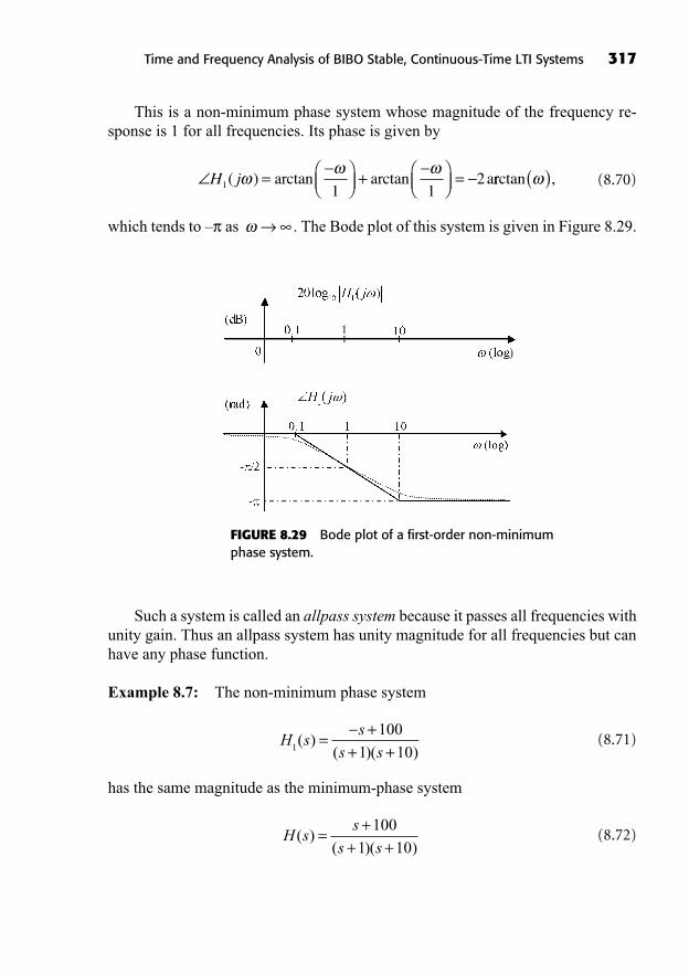
Time and Frequency Analysis of BIBO Stable, Continuous-Time LTI Systems 317
This is a non-minimum phase system whose magnitude of the frequency re-sponse is 1 for all frequencies. Its phase is given by
(8.70)
which tends to – as . The Bode plot of this system is given in Figure 8.29.
= + =H j1 1 12( ) arctan arctan arrctan ,( )
FIGURE 8.29 Bode plot of a first-order non-minimumphase system.
Such a system is called an allpass system because it passes all frequencies withunity gain. Thus an allpass system has unity magnitude for all frequencies but canhave any phase function.
Example 8.7: The non-minimum phase system
(8.71)
has the same magnitude as the minimum-phase system
(8.72)H ss
s s( )
( )( )=
++ +
100
1 10
H ss
s s1
100
1 10( )
( )( )=
++ +
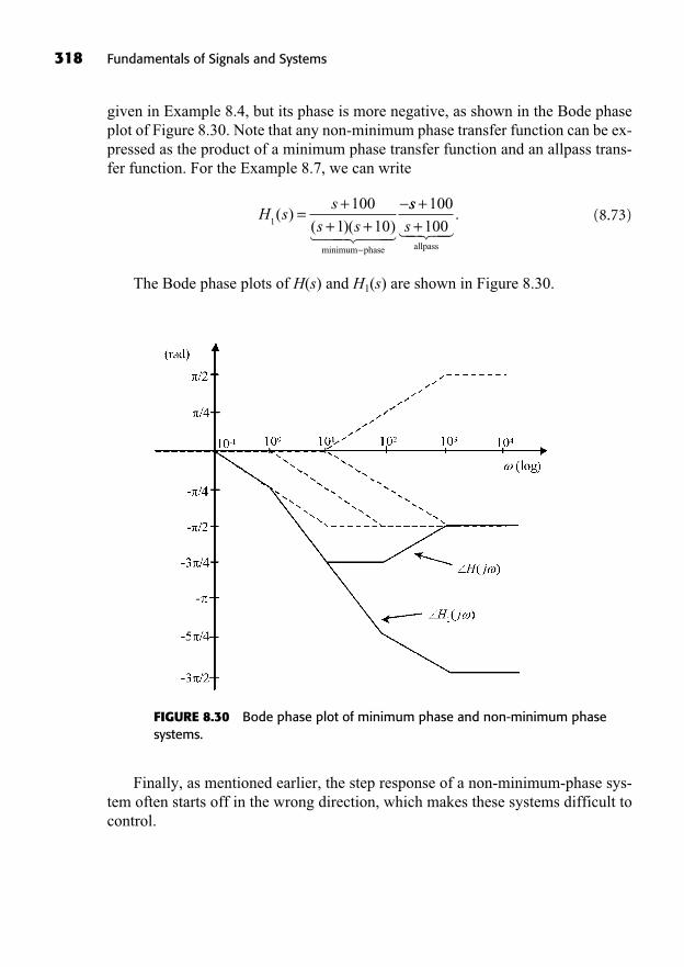
318 Fundamentals of Signals and Systems
given in Example 8.4, but its phase is more negative, as shown in the Bode phaseplot of Figure 8.30. Note that any non-minimum phase transfer function can be ex-pressed as the product of a minimum phase transfer function and an allpass trans-fer function. For the Example 8.7, we can write
(8.73)
The Bode phase plots of H(s) and H1(s) are shown in Figure 8.30.
H ss
s s1
100
1 10( )
( )( )=
++ +
minimum phase� ��� ���
ss
s
++
100
100allpass��� ��
.
FIGURE 8.30 Bode phase plot of minimum phase and non-minimum phasesystems.
Finally, as mentioned earlier, the step response of a non-minimum-phase sys-tem often starts off in the wrong direction, which makes these systems difficult tocontrol.
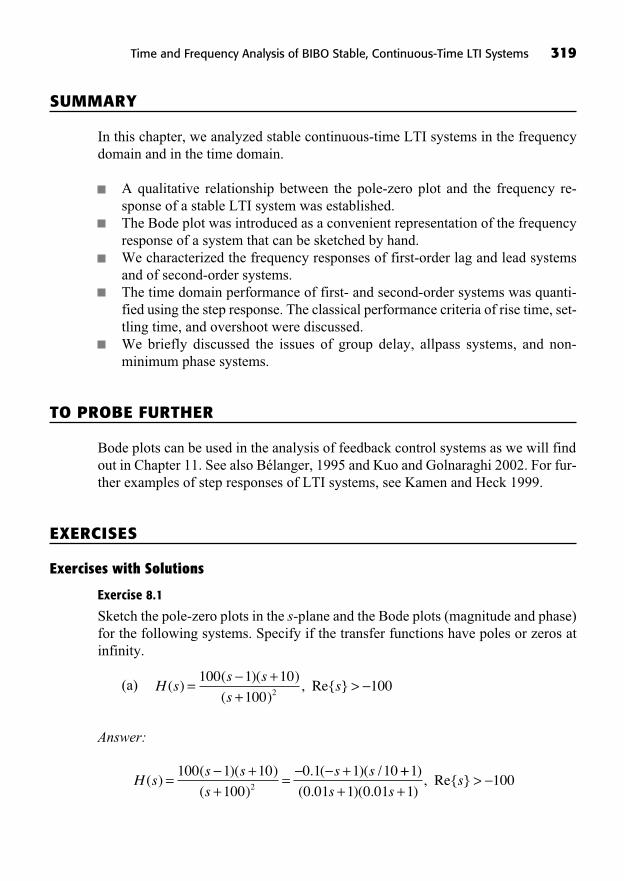
SUMMARY
In this chapter, we analyzed stable continuous-time LTI systems in the frequencydomain and in the time domain.
A qualitative relationship between the pole-zero plot and the frequency re-sponse of a stable LTI system was established.The Bode plot was introduced as a convenient representation of the frequencyresponse of a system that can be sketched by hand.We characterized the frequency responses of first-order lag and lead systemsand of second-order systems.The time domain performance of first- and second-order systems was quanti-fied using the step response. The classical performance criteria of rise time, set-tling time, and overshoot were discussed.We briefly discussed the issues of group delay, allpass systems, and non-minimum phase systems.
TO PROBE FURTHER
Bode plots can be used in the analysis of feedback control systems as we will findout in Chapter 11. See also Bélanger, 1995 and Kuo and Golnaraghi 2002. For fur-ther examples of step responses of LTI systems, see Kamen and Heck 1999.
EXERCISES
Exercises with Solutions
Exercise 8.1
Sketch the pole-zero plots in the s-plane and the Bode plots (magnitude and phase)for the following systems. Specify if the transfer functions have poles or zeros atinfinity.
(a)
Answer:
H ss s
s
s s( )
( )( )
( )
. ( )( /=
++
=+100 1 10
100
0 1 1 102
+++ +
>1
0 01 1 0 01 1100
)
( . )( . ), Re{ }
s ss
H ss s
ss( )
( )( )
( ), Re{ }=
++
>100 1 10
1001002
Time and Frequency Analysis of BIBO Stable, Continuous-Time LTI Systems 319

The break frequencies are at .The pole-zero plot is shown in Figure 8.31, and the Bode plot is shown in Figure 8.32.
(b) H ss
s ss( )
( . ), Re{ }=
++
>10
0 001 10
1 2 31 10 100= = =, (zeros); (double pole)
320 Fundamentals of Signals and Systems
FIGURE 8.31 Pole-zero plot of the transferfunction of Exercise 8.1(a).
FIGURE 8.32 Bode plot of the transfer functionof Exercise 8.1(a).
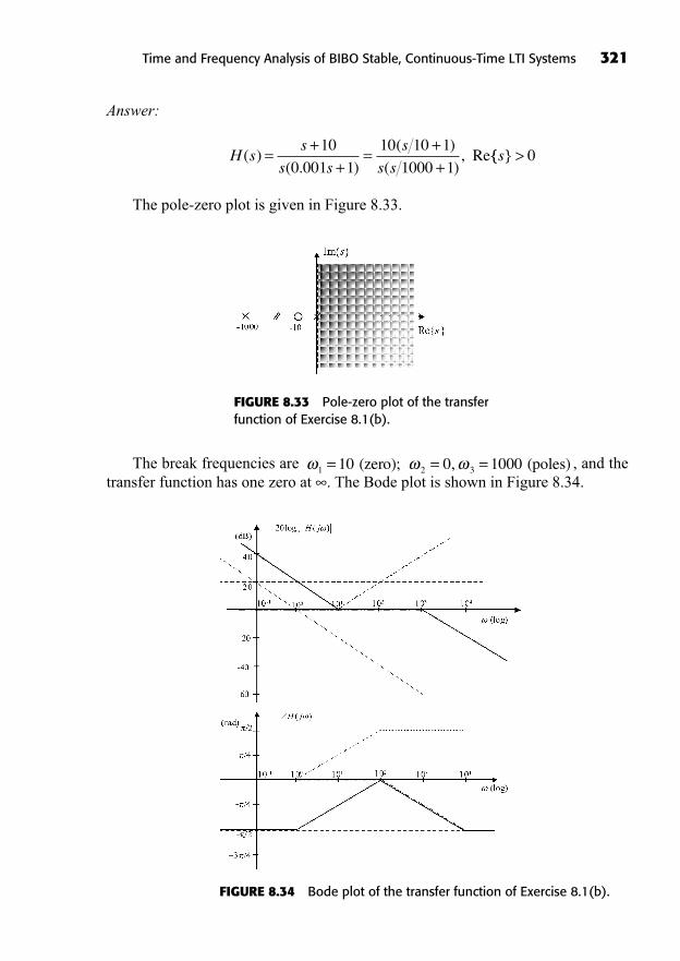
Answer:
The pole-zero plot is given in Figure 8.33.
H ss
s s
s
s s( )
( . )
( )
( ), Re=
++
=++
10
0 001 1
10 10 1
1000 1{{ }s > 0
Time and Frequency Analysis of BIBO Stable, Continuous-Time LTI Systems 321
FIGURE 8.33 Pole-zero plot of the transferfunction of Exercise 8.1(b).
The break frequencies are , and thetransfer function has one zero at . The Bode plot is shown in Figure 8.34.
1 2 310 0 1000= = = (zero); (poles),
FIGURE 8.34 Bode plot of the transfer function of Exercise 8.1(b).
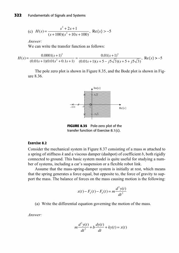
322 Fundamentals of Signals and Systems
(c)
Answer:We can write the transfer function as follows:
The pole zero plot is shown in Figure 8.35, and the Bode plot is shown in Fig-ure 8.36.
H ss
s s s( )
. ( )
( . )( . . )=
++ + +
=0 0001 1
0 01 1 0 01 0 1 1
02
2
.. ( )
( . )( )( ), Re{ }
01 1
0 01 1 5 5 3 5 5 3
2s
s s j s js
++ + + +
>> 5
H ss s
s s ss( )
( )( ), Re{ }=
+ ++ + +
>2
2
2 1
100 10 1005
FIGURE 8.35 Pole-zero plot of thetransfer function of Exercise 8.1(c).
Exercise 8.2
Consider the mechanical system in Figure 8.37 consisting of a mass m attached toa spring of stiffness k and a viscous damper (dashpot) of coefficient b, both rigidlyconnected to ground. This basic system model is quite useful for studying a num-ber of systems, including a car’s suspension or a flexible robot link.
Assume that the mass-spring-damper system is initially at rest, which meansthat the spring generates a force equal, but opposite to, the force of gravity to sup-port the mass. The balance of forces on the mass causing motion is the following:
(a) Write the differential equation governing the motion of the mass.
Answer:
md y t
dtbdy t
dtky t x t
2
2
( ) ( )( ) ( )+ + =
x t F t F t md y t
dtk b( ) ( ) ( )( )
=2
2

Time and Frequency Analysis of BIBO Stable, Continuous-Time LTI Systems 323
FIGURE 8.36 Bode plot of the transfer function of Exercise 8.1(c).
FIGURE 8.37 Mass-spring-damper system of Exercise 8.2.
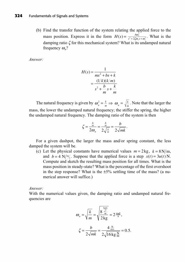
(b) Find the transfer function of the system relating the applied force to the
mass position. Express it in the form . What is the
damping ratio for this mechanical system? What is its undamped naturalfrequency n?
Answer:
The natural frequency is given by . Note that the larger the
mass, the lower the undamped natural frequency; the stiffer the spring, the higherthe undamped natural frequency. The damping ratio of the system is then
For a given dashpot, the larger the mass and/or spring constant, the lessdamped the system will be.
(c) Let the physical constants have numerical values , ,and . Suppose that the applied force is a step .Compute and sketch the resulting mass position for all times. What is themass position in steady-state? What is the percentage of the first overshootin the step response? What is the ±5% settling time of the mass? (a nu-merical answer will suffice.)
Answer:With the numerical values given, the damping ratio and undamped natural fre-quencies are
= = =b
mk2
4
2 160 5
Nm/s
kg Nm
. .
n
k
m= = =
8
22
kgm
s2
m
kgrads ,
x t u t( ) ( )= 3 Nb = 4 N ms
k = 8N mm = 2kg
= = =bm
n
bm
km
b
mk2 2 2.
k
mn=k
mn2 =
H sms bs k
k k m
sbms
km
( )
( )( )
=+ +
=+ +
1
1
2
2
A
s sn
n n+ +
2
2 22H s( ) =
324 Fundamentals of Signals and Systems
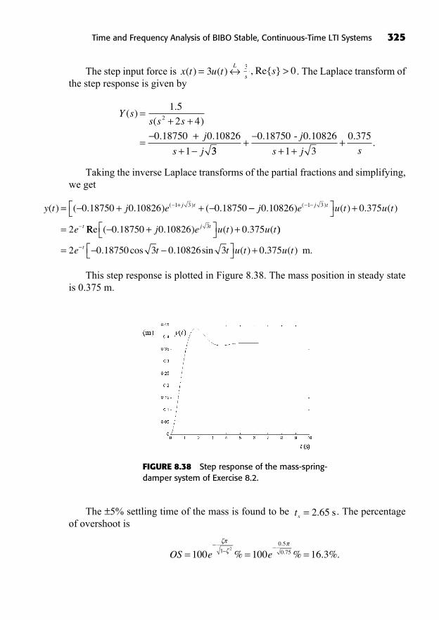
Time and Frequency Analysis of BIBO Stable, Continuous-Time LTI Systems 325
The step input force is . The Laplace transform ofthe step response is given by
Taking the inverse Laplace transforms of the partial fractions and simplifying,we get
This step response is plotted in Figure 8.38. The mass position in steady stateis 0.375 m.
y t j e j t( ) ( . . ) ( .( )= + ++0 18750 0 10826 0 187501 3 +
=
j e u t u t
e
j t
t
0 10826 0 375
2
1 3. ) ( ) . ( )( )
RRe ( . . ) ( ) . (+ +0 18750 0 10826 0 3753j e u t u tj t ))
. cos . sin ( )= +2 0 18750 3 0 10826 3 0e t t u tt .. ( )375u t m.
Y ss s s
j
s j
( ).
( )
. .
=+ +
=+
+
1 5
2 4
0 18750 0 10826
1
2
33
0 18750 0 10826
1 3+
+ ++
. ..
- 0.375j
s j s
s, Re{ } > 0s
3x t u tL
( ) ( )= 3
FIGURE 8.38 Step response of the mass-spring-damper system of Exercise 8.2.
The ±5% settling time of the mass is found to be . The percentageof overshoot is
OS e e= = =100 100 16 310 5
0 752
% % . %..
.
ts = 2 65. s
326 Fundamentals of Signals and Systems
Exercises
Exercise 8.3
Compute the 95% rise time tr and the ±5% settling time ts of the step response ofthe system .
Answer:
Exercise 8.4
Compute the DC gain in decibels, the peak resonance in decibels, and the qualityQ of the second-order causal filter with transfer function .
Exercise 8.5
Compute the actual value of the first overshoot in the step response of the causalLTI system
Answer:
Exercise 8.6
Compute the group delay of a communication channel represented by the causalfirst-order system . Compute the approximate valueof the channel’s delay at very low frequencies.
Exercise 8.7
Sketch the pole-zero plots in the s-plane and the Bode plots (magnitude and phase)for the following systems. Specify whether the transfer functions have poles orzeros at infinity.
(a)
(b) H ss
s ss( )
( . ), Re{ }=
++
>10
0 005 10
H ss
s ss( )
( )
( )( ), Re{ }=
+ +>
100 20
5 10052
s, Re{ } > 100s. +
1
0 01 1H s( ) =
H ss s
( ) .=+ +
5
3 3 62
s s+ +1000
2 1002H s( ) =
s, Re{ } > 10s
s
.
.
++
0 001 1
0 1 1H s( ) =
Time and Frequency Analysis of BIBO Stable, Continuous-Time LTI Systems 327
(c)
Answer:
Exercise 8.8
Sketch the pole-zero plots in the s-plane and the Bode plots (magnitude and phase)for the following systems. Specify if the transfer functions have poles or zeros atinfinity.
(a)
(b)
(c)
Exercise 8.9
Consider the causal differential system described by
with initial conditions . Suppose that this system is subjectedto the input signal .
(a) Find the system’s damping ratio and undamped natural frequency n.Compute the output of the system y(t) for t ≥ 0. Find the steady-state re-sponse yss(t), the transient response ytr(t), the zero-input response yzi(t), andthe zero-state response yzs(t) for t ≥ 0.
(b) Plot yss(t), ytr(t), yzi(t), and yzs(t) for t ≥ 0, all on the same figure usingMATLAB or any other software of your choice.
(c) Find the frequency response of the system and sketch its Bode plot.
Answer:
x t e u tt( ) ( )= 2y, ( )3 0 0= =dy
dt
( )0
1
4
1
2
2
2
d y t
dt
dy t
dty t
dx t
dtx t
( ) ( )( )
( )( ),+ + = +
H ss s
s s ss( )
( )
( )( ), Re{ }=
+ + +>
2
2
9
100 10 1005
H ss
s ss( )
( . ), Re{ }=
++
>1
0 01 10
H ss
s s ss( )
( )
( )( )( ), Re{ }=
+ + +>
100 10
1 10 1001
H ss
s ss( ) , Re{ }=
+ +>
2
2 30 90015
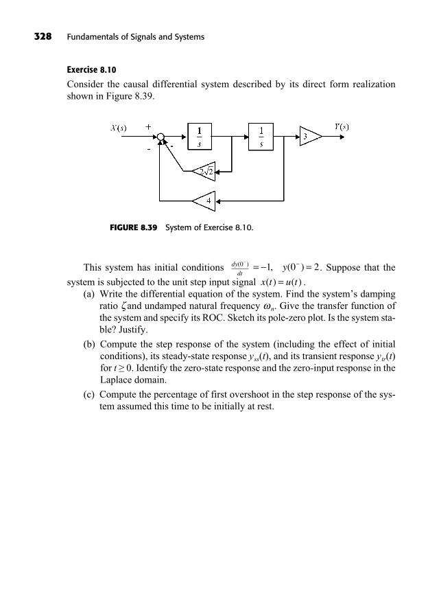
328 Fundamentals of Signals and Systems
Exercise 8.10
Consider the causal differential system described by its direct form realizationshown in Figure 8.39.
FIGURE 8.39 System of Exercise 8.10.
This system has initial conditions . Suppose that the
system is subjected to the unit step input signal .(a) Write the differential equation of the system. Find the system’s damping
ratio and undamped natural frequency n. Give the transfer function ofthe system and specify its ROC. Sketch its pole-zero plot. Is the system sta-ble? Justify.
(b) Compute the step response of the system (including the effect of initialconditions), its steady-state response yss(t), and its transient response ytr(t)for t ≥ 0. Identify the zero-state response and the zero-input response in theLaplace domain.
(c) Compute the percentage of first overshoot in the step response of the sys-tem assumed this time to be initially at rest.
x t u t( ) ( )=y, ( )1 0 2= =dy
dt
( )0

329
Application of LaplaceTransform Techniques toElectric Circuit Analysis
9
In This Chapter
Review of Nodal Analysis and Mesh Analysis of CircuitsTransform Circuit Diagrams: Transient and Steady-State AnalysisOperational Amplifier CircuitsSummaryTo Probe FurtherExercises
((Lecture 31: Review of Nodal Analysis and Mesh Analysis of Circuits))
The Laplace transform is a very useful tool for analyzing linear time-invariant(LTI) electric circuits. It can be used to solve the differential equation relat-ing an input voltage or current signal to another output signal in the circuit.
It can also be used to analyze the circuit directly in the Laplace domain, where cir-cuit components are replaced by their impedances seen as transfer functions.
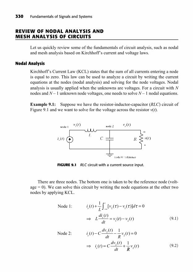
330 Fundamentals of Signals and Systems
REVIEW OF NODAL ANALYSIS AND MESH ANALYSIS OF CIRCUITS
Let us quickly review some of the fundamentals of circuit analysis, such as nodaland mesh analysis based on Kirchhoff’s current and voltage laws.
Nodal Analysis
Kirchhoff’s Current Law (KCL) states that the sum of all currents entering a nodeis equal to zero. This law can be used to analyze a circuit by writing the currentequations at the nodes (nodal analysis) and solving for the node voltages. Nodalanalysis is usually applied when the unknowns are voltages. For a circuit with Nnodes and N – 1 unknown node voltages, one needs to solve N – 1 nodal equations.
Example 9.1: Suppose we have the resistor-inductor-capacitor (RLC) circuit ofFigure 9.1 and we want to solve for the voltage across the resistor v(t).
Node 1:
Node 2:
FIGURE 9.1 RLC circuit with a current source input.
There are three nodes. The bottom one is taken to be the reference node (volt-age = 0). We can solve this circuit by writing the node equations at the other twonodes by applying KCL.
(9.1)
(9.2)
i t Cdv t
dt Rv t
i t Cdv t
dt
s
s
( )( )
( )
( )( )
=
= +
22
2
10
1
RRv t
2( )
i tL
v v d
Ldi t
dtv
s
t
s
( ) [ ( ) ( )]
( )(
+ =
=
10
2 1
1tt v t) ( )
2
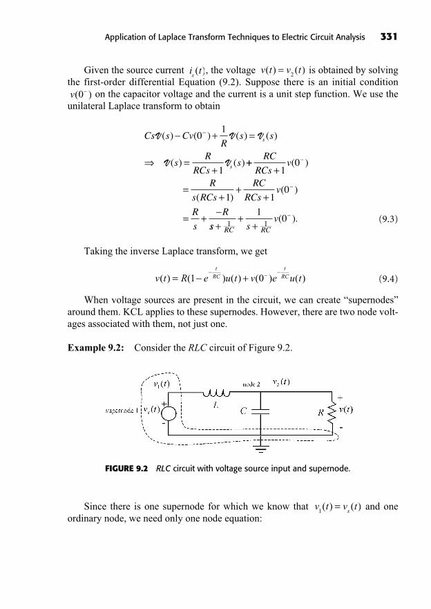
Given the source current , the voltage is obtained by solvingthe first-order differential Equation (9.2). Suppose there is an initial condition
on the capacitor voltage and the current is a unit step function. We use theunilateral Laplace transform to obtain
(9.3)
Taking the inverse Laplace transform, we get
(9.4)
When voltage sources are present in the circuit, we can create “supernodes”around them. KCL applies to these supernodes. However, there are two node volt-ages associated with them, not just one.
Example 9.2: Consider the RLC circuit of Figure 9.2.
v t R e u t v e u tt
RCt
RC( ) ( ) ( ) ( ) ( )= +1 0
Cs s CvR
s s
sR
RCss
s
s
V V V
V V
( ) ( ) ( ) ( )
( ) ( )
+ =
=+
01
1++
+
=+
++
= +
RC
RCsv
R
s RCs
RC
RCsv
R
s
R
10
1 10
( )
( )( )
ss sv
RC RC++
+1 1
10( ).
v( )0
v t v t( ) ( )=2i t
s( )
Application of Laplace Transform Techniques to Electric Circuit Analysis 331
FIGURE 9.2 RLC circuit with voltage source input and supernode.
Since there is one supernode for which we know that and oneordinary node, we need only one node equation:
v t v ts1
( ) ( )=

332 Fundamentals of Signals and Systems
(9.5)
Mesh Analysis
Kirchhoff’s Voltage Law (KVL) states that the sum of all voltages around a mesh(a loop that has no element within it) is equal to zero. This law can be used to an-alyze a circuit by writing the voltage equation for each mesh (mesh analysis) andsolving for the mesh currents. Mesh analysis is usually applied when the unknownsare currents.
Example 9.3: Suppose that we have the circuit in Figure 9.3 and we want tosolve for the current flowing in the capacitor.i t i t i t( ) ( ) ( )=
1 2
1 10
1
22
2Lv v d C
dv t
dt Rv t
t
s[ ( ) ( )]
( )( ) =
LLv t v t C
d v t
dt R
dv t
dt
v t
s
s
[ ( ) ( )]( ) ( )
( )
= +2
222
21
== + +LCd v t
dt
L
R
dv t
dtv t
222
22
( ) ( )( )
Node 1:
FIGURE 9.3 RLC circuit with voltage source input andmesh currents
Mesh 1:
(9.6)
Mesh 2:
(9.7)
10
1
1 2 2
1 2
Ci i d Ri t
Ci t i
t[ ( ) ( )] ( )
[ ( ) (
=
tt Rdi t
dt)]
( )= 2
v t Ldi t
dt Ci i d
C
s
t( )
( )[ ( ) ( )]
[
=11 2
10
1ii t i t L
d i t
dt
dv t
dts
1 2
21
2( ) ( )]
( ) ( )+ =
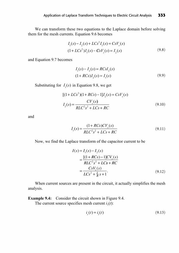
We can transform these two equations to the Laplace domain before solvingthem for the mesh currents. Equation 9.6 becomes
(9.8)
and Equation 9.7 becomes
(9.9)
Substituting for in Equation 9.8, we get
(9.10)
and
(9.11)
Now, we find the Laplace transform of the capacitor current to be
(9.12)
When current sources are present in the circuit, it actually simplifies the meshanalysis.
Example 9.4: Consider the circuit shown in Figure 9.4.The current source specifies mesh current i1(t):
(9.13)i t i ts( ) ( )=
1
I s I s I s
RCs CV s
RLC s LCs
( ) ( ) ( )
[( ) ] ( )
=
=+
+
1 2
2 2
1 1
ss RCCsV s
LCs ss
LR
+
=+ +
( ).2 1
I sRCs CV s
RLC s LCs RCs
1 2 2
1( )
( ) ( )=
++ +
[( )( ) ] ( ) ( )
( )(
1 1 122
2
+ + =
=
LCs RCs I s CsV s
I sCV s
s
s))
RLC s LCs RC2 2 + +
I s1( )
I s I s RCsI s
RCs I s I s1 2 2
2 11
( ) ( ) ( )
( ) ( ) ( )
=+ =
I s I s LCs I s CsV s
LCs I ss1 2
21
21
1
( ) ( ) ( ) ( )
( ) ( )
+ =
+ CCsV s I ss( ) ( )=
2
Application of Laplace Transform Techniques to Electric Circuit Analysis 333
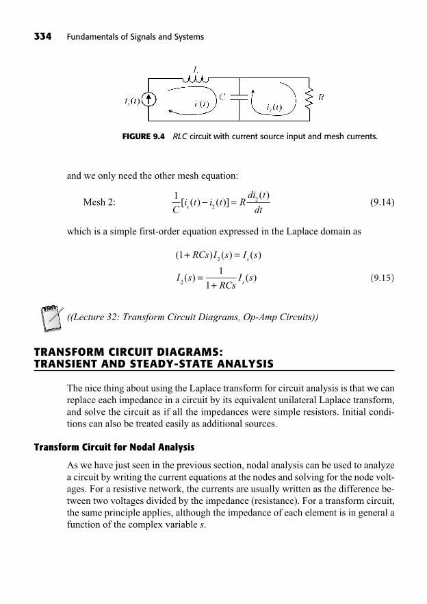
334 Fundamentals of Signals and Systems
and we only need the other mesh equation:
Mesh 2: (9.14)
which is a simple first-order equation expressed in the Laplace domain as
(9.15)
((Lecture 32: Transform Circuit Diagrams, Op-Amp Circuits))
TRANSFORM CIRCUIT DIAGRAMS: TRANSIENT AND STEADY-STATE ANALYSIS
The nice thing about using the Laplace transform for circuit analysis is that we canreplace each impedance in a circuit by its equivalent unilateral Laplace transform,and solve the circuit as if all the impedances were simple resistors. Initial condi-tions can also be treated easily as additional sources.
Transform Circuit for Nodal Analysis
As we have just seen in the previous section, nodal analysis can be used to analyzea circuit by writing the current equations at the nodes and solving for the node volt-ages. For a resistive network, the currents are usually written as the difference be-tween two voltages divided by the impedance (resistance). For a transform circuit,the same principle applies, although the impedance of each element is in general afunction of the complex variable s.
( ) ( ) ( )
( ) ( )
1
1
1
2
2
+ =
=+
RCs I s I s
I sRCs
I s
s
s
12
2
Ci t i t R
di t
dts[ ( ) ( )]
( )=
FIGURE 9.4 RLC circuit with current source input and mesh currents.
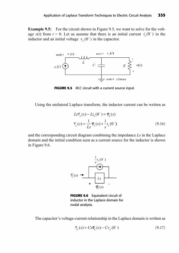
Example 9.5: For the circuit shown in Figure 9.5, we want to solve for the volt-age v(t) from t = 0. Let us assume that there is an initial current in theinductor and an initial voltage in the capacitor.v
C( )0
iL( )0
Application of Laplace Transform Techniques to Electric Circuit Analysis 335
FIGURE 9.5 RLC circuit with a current source input.
Using the unilateral Laplace transform, the inductor current can be written as
(9.16)
and the corresponding circuit diagram combining the impedance Ls in the Laplacedomain and the initial condition seen as a current source for the inductor is shownin Figure 9.6.
Ls s Li s
sLs
ss
i
L L L
L L L
I V
I V
( ) ( ) ( )
( ) ( ) (
=
= +
0
1 10 ))
FIGURE 9.6 Equivalent circuit ofinductor in the Laplace domain fornodal analysis.
The capacitor’s voltage-current relationship in the Laplace domain is written as
(9.17)I VC C C
s Cs s Cv( ) ( ) ( )= 0

336 Fundamentals of Signals and Systems
and the corresponding circuit diagram combining the impedance in the Laplacedomain and the initial condition seen as a current source for the capacitor is givenin Figure 9.7.
1
Cs
FIGURE 9.7 Equivalent circuit ofthe capacitor in the Laplace domainfor nodal analysis.
A resistor of resistance R is just an impedance R in the Laplace domain. Withthese impedances and equivalent current sources defined, the transform circuit isdepicted in Figure 9.8.
FIGURE 9.8 Transform circuit diagram with current source.
We can solve this circuit by writing the node equations.
Node 1:
(9.18)
I V V
V I
s Ls
Lss s
si
s Ls
( ) [ ( ) ( )] ( )
( )
+ =
=
1 10 0
2 1
1 ss Ls s Li( ) ( ) ( )+ V
20
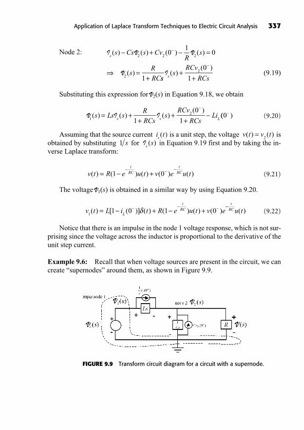
Node 2:
(9.19)
Substituting this expression for V2(s) in Equation 9.18, we obtain
(9.20)
Assuming that the source current is a unit step, the voltage isobtained by substituting for in Equation 9.19 first and by taking the in-verse Laplace transform:
(9.21)
The voltage V1(s) is obtained in a similar way by using Equation 9.20.
(9.22)
Notice that there is an impulse in the node 1 voltage response, which is not sur-prising since the voltage across the inductor is proportional to the derivative of theunit step current.
Example 9.6: Recall that when voltage sources are present in the circuit, we cancreate “supernodes” around them, as shown in Figure 9.9.
v t L i t R e u t v eL
tRC
11 0 1 0( ) [ ( )] ( ) ( ) ( ) ( )= + +
tRC u t( )
v t R e u t v e u tt
RCt
RC( ) ( ) ( ) ( ) ( )= +1 0
Is
s( )1 sv t v t( ) ( )=
2i ts( )
V I I1
2
1
0
1( ) ( ) ( )
( )s Ls s
R
RCss
RCv
RCsLi
s s L= +
++
+(( )0
I V V
V
ss Cs s Cv
Rs
sR
RC
( ) ( ) ( ) ( )
( )
+ =
=+
2 2 2
2
01
0
1 sss
RCv
RCssI ( )
( )+
+2
0
1
Application of Laplace Transform Techniques to Electric Circuit Analysis 337
FIGURE 9.9 Transform circuit diagram for a circuit with a supernode.
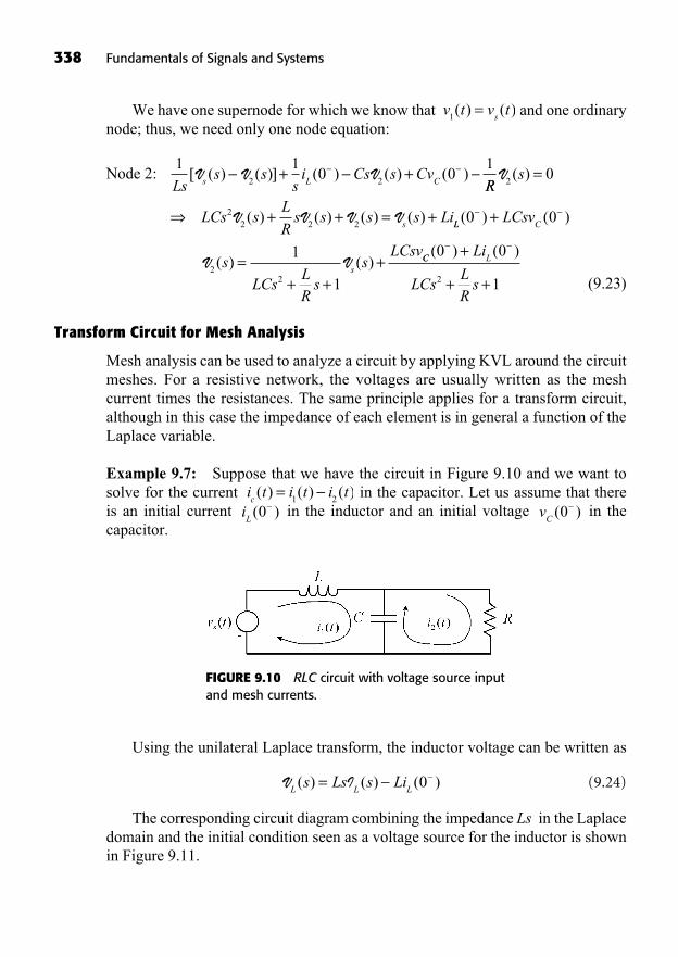
338 Fundamentals of Signals and Systems
We have one supernode for which we know that and one ordinarynode; thus, we need only one node equation:
Node 2:
(9.23)
Transform Circuit for Mesh Analysis
Mesh analysis can be used to analyze a circuit by applying KVL around the circuitmeshes. For a resistive network, the voltages are usually written as the meshcurrent times the resistances. The same principle applies for a transform circuit,although in this case the impedance of each element is in general a function of theLaplace variable.
Example 9.7: Suppose that we have the circuit in Figure 9.10 and we want tosolve for the current in the capacitor. Let us assume that there is an initial current in the inductor and an initial voltage in the capacitor.
vC
( )0iL( )0
i t i t i tc( ) ( ) ( )=
1 2
1 10 0
12 2Ls
s ss
i Cs s Cvs L C
[ ( ) ( )] ( ) ( ) ( )V V V+ +RR
s
LCs sL
Rs s s s Li
s
V
V V V V
2
22 2 2
0( )
( ) ( ) ( ) ( )
=
+ + = +LL C
s
LCsv
sLCs
LR
ss
LCsv
( ) ( )
( ) ( )
0 0
1
12
2
+
=+ +
+V V CC LLi
LCsLR
s
( ) ( )0 0
12
+
+ +
v t v ts1
( ) ( )=
FIGURE 9.10 RLC circuit with voltage source inputand mesh currents.
Using the unilateral Laplace transform, the inductor voltage can be written as
(9.24)
The corresponding circuit diagram combining the impedance Ls in the Laplacedomain and the initial condition seen as a voltage source for the inductor is shownin Figure 9.11.
V IL L L
s Ls s Li( ) ( ) ( )= 0

The capacitor voltage-current relationship in the Laplace domain is written as
(9.25)
The corresponding circuit diagram combining the impedance in the Laplacedomain and the initial condition seen as a voltage source for the capacitor is asshown in Figure 9.12.
1
Cs
V IC C C
sCs
ss
v( ) ( ) ( )= +1 1
0
Application of Laplace Transform Techniques to Electric Circuit Analysis 339
FIGURE 9.11 Equivalent circuit of inductorin the Laplace domain for mesh analysis.
FIGURE 9.12 Equivalent circuit ofcapacitor in the Laplace domain formesh analysis.
With these impedances and equivalent current sources defined, the transformcircuit can be depicted as in Figure 9.13.
FIGURE 9.13 Transform RLC circuit with voltage sourcesfor the input and initial conditions and with mesh currentsin the Laplace domain.
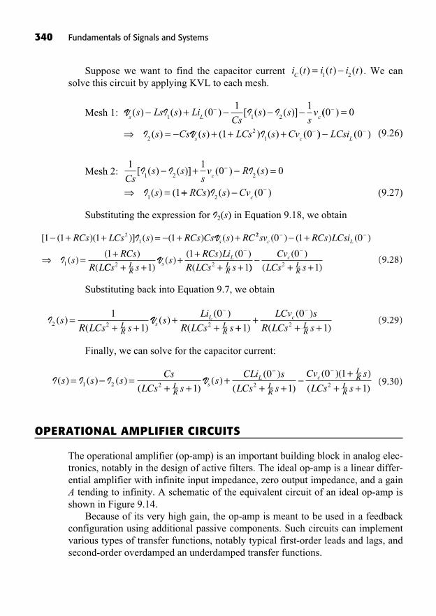
Suppose we want to find the capacitor current . We cansolve this circuit by applying KVL to each mesh.
Mesh 1:
(9.26)
Mesh 2:
(9.27)
Substituting the expression for I2(s) in Equation 9.18, we obtain
(9.28)
Substituting back into Equation 9.7, we obtain
(9.29)
Finally, we can solve for the capacitor current:
(9.30)
OPERATIONAL AMPLIFIER CIRCUITS
The operational amplifier (op-amp) is an important building block in analog elec-tronics, notably in the design of active filters. The ideal op-amp is a linear differ-ential amplifier with infinite input impedance, zero output impedance, and a gainA tending to infinity. A schematic of the equivalent circuit of an ideal op-amp isshown in Figure 9.14.
Because of its very high gain, the op-amp is meant to be used in a feedbackconfiguration using additional passive components. Such circuits can implementvarious types of transfer functions, notably typical first-order leads and lags, andsecond-order overdamped an underdamped transfer functions.
I I I V( ) ( ) ( )( )
( )(
s s sCs
LCs ss
CLiLR
sL= =
+ ++1 2 2 1
0
+ ++
+ +)
( )
( )( )
( )
s
LCs s
Cv s
LCs sLR
LR
LR
c2 21
0 1
1
I V2 2 2
1
1
0( )
( )( )
( )
(s
R LCs ss
Li
R LCs sLR
LR
sL=
+ ++
+ +++
+ +1
0
12)
( )
( )
LCv s
R LCs sc
LR
[ ( )( )] ( ) ( ) ( )1 1 1 121+ + = + +RCs LCs s RCs Cs s RCsI V 22
1
0 1 0
1
sv RCs LCsi
sRCs
R L
c L( ) ( ) ( )
( )( )
(
+
=+
ICCs s
sRCs Li
R LCs sLR
LR
sL
2 21
1 0
1+ ++
++ +)
( )( ) ( )
(V
))
( )
( )+ +Cv
LCs sc
LR
0
12
1 10 0
1
1 2 2
1
Css s
sv R s
s
c[ ( ) ( )] ( ) ( )
( ) (
I I I
I
+ =
= ++ RCs s Cvc
) ( ) ( )I2
0
V I I Is L c
s Ls s LiCs
s ss
v( ) ( ) ( ) [ ( ) ( )]+1 1 2
01 1
(( )
( ) ( ) ( ) ( ) (
0 0
1 02
21
=
= + + +I V Is Cs s LCs s Cvs c
)) ( )LCsiL
0
i t i t i tC
( ) ( ) ( )=1 2
340 Fundamentals of Signals and Systems
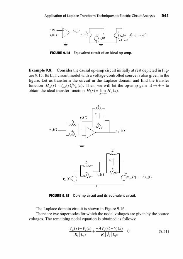
Application of Laplace Transform Techniques to Electric Circuit Analysis 341
Example 9.8: Consider the causal op-amp circuit initially at rest depicted in Fig-ure 9.15. Its LTI circuit model with a voltage-controlled source is also given in thefigure. Let us transform the circuit in the Laplace domain and find the transferfunction . Then, we will let the op-amp gain toobtain the ideal transfer function .H s H s
AA( ) lim ( )=
+
A +H s V s V sA out in( ) ( ) ( )=
FIGURE 9.14 Equivalent circuit of an ideal op-amp.
FIGURE 9.15 Op-amp circuit and its equivalent circuit.
The Laplace domain circuit is shown in Figure 9.16.There are two supernodes for which the nodal voltages are given by the source
voltages. The remaining nodal equation is obtained as follows:
(9.31)V s V s
R L s
AV s V s
R L sin x x x
Cs
( ) ( ) ( ) ( )+ =
2 2 1 11
0

342 Fundamentals of Signals and Systems
where = and are the resulting
impedances of the parallel connections of the individual impedances. Simplifyingthe above equation, we get
(9.32)
Thus, the transfer function between the input voltage and the node voltage isgiven by
(9.33)
and the transfer function between the input voltage and the output voltage can beobtained:
(9.34)
The ideal transfer function is obtained as the limit of Equation 9.34 as the op-amp gain tends to infinity:
(9.35)H s H sR L R L s
R L R L CsAA( ) lim ( )
( )
(= =
++
1 1 2 2
2 2 1 12 LL s R
LLRs
L L CsLRs1 1
12
2
2 12 1
1
1
1+=
+
+ +)
( )
( )
H sV s
V s
AV s
V s
AR L s RA
out
in
x
in
( )( )
( )
( )
( )
(= = = 1 1 22 2
2 2 1 12
1 1 1 1 21
++ + + + +
L s
R L s A R L Cs L s R R L s R
)
( )( ) ( LL s2 )
V s
V s
R L sR L s
A R L Cs L s Rx
in
( )
( ) ( )(=
+
+ + +
2 2
2 2
1 12
1 11 ))
( )
( )
R L sR L sR L s
R L s R L s
R L s A
1 1
2 2
2 2
1 1 2 2
2 2 1
+ +
=+
+ (( ) ( ),
R L Cs L s R R L s R L s1 12
1 1 1 1 2 2+ + + +
R L s
R L sV s
A R L Cs L s R
R Lin2 2
2 2
1 12
1 1
1 1
1+ + + +( )
( )( )
ss
R L s
R L sV sx+
+ =2 2
2 2
0( )
R L s
R L s2 2
2 2+R L s2 2 =R L s
R L Cs L s R1 1
1 12
1 1+ +Cs R L s1 1
1
1 1+ +R L sCs1 1
1 =
FIGURE 9.16 Laplace transform circuit.
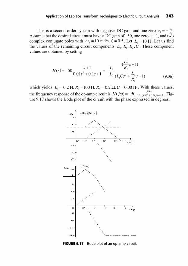
This is a second-order system with negative DC gain and one zero .Assume that the desired circuit must have a DC gain of –50, one zero at –1, and twocomplex conjugate poles with . Let . Let us findthe values of the remaining circuit components . These componentvalues are obtained by setting
(9.36)
which yields . With these values,
the frequency response of the op-amp circuit is . Fig-ure 9.17 shows the Bode plot of the circuit with the phase expressed in degrees.
j
j j. ( ) . ( )
++ +
1
0 01 0 1 12H j( ) = 50
L R R C2 1 20 2 100 0 2 0 001= = = =. , , . , .H F
H ss
s s
L
L
LRs
L C( )
. .
( )
(=
++ +
=+
501
0 01 0 1 1
1
21
2
2
2
1 ssLRs2 1
1
1+ + )
L R R C2 1 2, , ,L1 10= Hn = =10 0 5 rad/s, .
R
L2
2
z1 =
Application of Laplace Transform Techniques to Electric Circuit Analysis 343
FIGURE 9.17 Bode plot of an op-amp circuit.
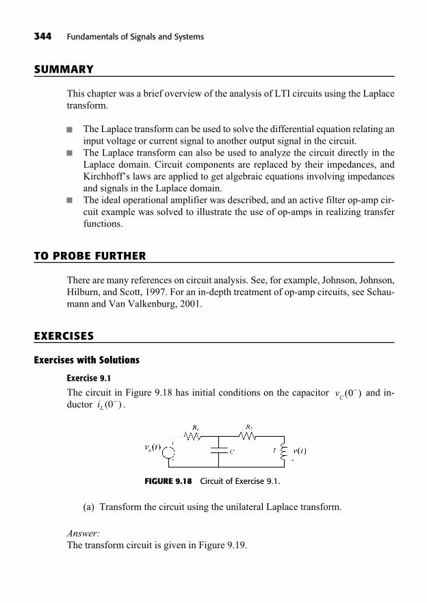
344 Fundamentals of Signals and Systems
SUMMARY
This chapter was a brief overview of the analysis of LTI circuits using the Laplacetransform.
The Laplace transform can be used to solve the differential equation relating aninput voltage or current signal to another output signal in the circuit.The Laplace transform can also be used to analyze the circuit directly in theLaplace domain. Circuit components are replaced by their impedances, andKirchhoff’s laws are applied to get algebraic equations involving impedancesand signals in the Laplace domain.The ideal operational amplifier was described, and an active filter op-amp cir-cuit example was solved to illustrate the use of op-amps in realizing transferfunctions.
TO PROBE FURTHER
There are many references on circuit analysis. See, for example, Johnson, Johnson,Hilburn, and Scott, 1997. For an in-depth treatment of op-amp circuits, see Schau-mann and Van Valkenburg, 2001.
EXERCISES
Exercises with Solutions
Exercise 9.1
The circuit in Figure 9.18 has initial conditions on the capacitor and in-ductor .iL ( )0
vC
( )0
FIGURE 9.18 Circuit of Exercise 9.1.
(a) Transform the circuit using the unilateral Laplace transform.
Answer:The transform circuit is given in Figure 9.19.
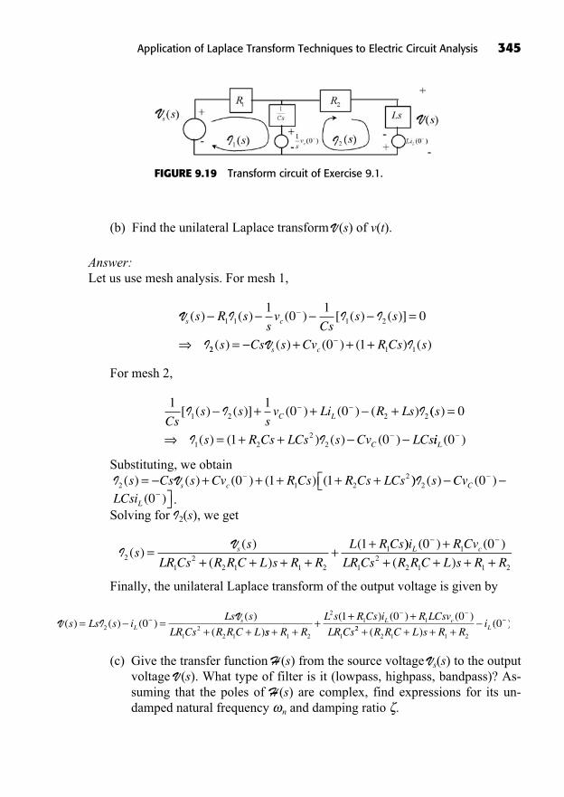
(b) Find the unilateral Laplace transform V (s) of v(t).
Answer:Let us use mesh analysis. For mesh 1,
For mesh 2,
Substituting, we obtain
.Solving for I2(s), we get
Finally, the unilateral Laplace transform of the output voltage is given by
(c) Give the transfer function H (s) from the source voltage Vs(s) to the outputvoltage V (s). What type of filter is it (lowpass, highpass, bandpass)? As-suming that the poles of H (s) are complex, find expressions for its un-damped natural frequency n and damping ratio .
V IV
( ) ( ) ( )( )
( )s Ls s i
Ls s
LR Cs R R C LLs= =
+ +2 01
22 1 ss R R
L s R Cs i R LCsv
LR CsL c
+ ++
+ +
1 2
21 1
1
1 0 0( ) ( ) ( )22
2 1 1 2
0+ + + +( )
( )R R C L s R R
iL
IV
21
22 1 1 2
11( )
( )
( )
(s
s
LR Cs R R C L s R R
L R Css=+ + + +
++ )) ( ) ( )
( )
i R Cv
LR Cs R R C L s R RL c0 01
12
2 1 1 2
++ + + +
( )0LCsiL
I V2 1 220 1 1( ) ( ) ( ) ( ) (s Cs s Cv R Cs R Cs LCss c= + + + + + )) ( ) ( )I2 0s CvC
1 10 01 2 2 2Cs
s ssv Li R LsC L[ ( ) ( )] ( ) ( ) ( )I I I+ + + (( )
( ) ( ) ( ) ( )
s
s R Cs LCs s Cv LCsC
=
= + +
0
1 01 22
2I I iiL ( )0
V I I I
I
s cs R ssv
Css s( ) ( ) ( ) [ ( ) ( )] =1 1 1 2
10
10
22 1 10 1( ) ( ) ( ) ( ) ( )s Cs s Cv R Cs ss c= + + +V I
Application of Laplace Transform Techniques to Electric Circuit Analysis 345
FIGURE 9.19 Transform circuit of Exercise 9.1.
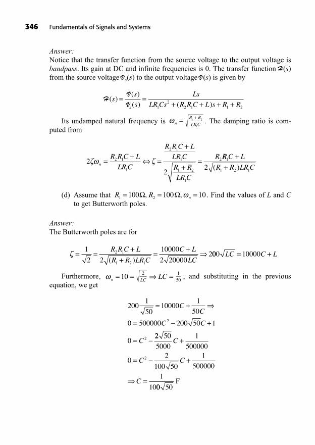
Answer:Notice that the transfer function from the source voltage to the output voltage isbandpass. Its gain at DC and infinite frequencies is 0. The transfer function H(s)from the source voltage V s(s) to the output voltage V (s) is given by
Its undamped natural frequency is . The damping ratio is com-puted from
(d) Assume that . Find the values of L and Cto get Butterworth poles.
Answer:The Butterworth poles are for
Furthermore, , and substituting in the previousequation, we get
2001
5010000
1
50
0 500000 200 50 1
0
2
2
= +
= +
=
CC
C C
C22 50
5000
1
500000
02
100 50
1
5000001
10
2
C
C C
C
+
= +
=00 50
F
1
50LC =LC
2n = =10
= =+
+=
+1
2 2
10000
2 2000022 1
1 2 1
R R C L
R R LR C
C L
LC( )000 10000LC C L= +
R R n1 2100 100 10= = =, ,
2
2
2 1
1
2 1
1
1 2
1
2n
R R C L
LR C
R R C LLR C
R RLR C
R=
+=
+
+=
RR C L
R R LR C1
1 2 12
++( )
R R
LR C
+1 2
1n =
HVV
( )( )
( ) ( )s
s
s
Ls
LR Cs R R C L s R Rs
= =+ + + +1
22 1 1 2
346 Fundamentals of Signals and Systems
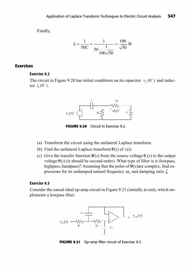
Application of Laplace Transform Techniques to Electric Circuit Analysis 347
Finally,
Exercises
Exercise 9.2
The circuit in Figure 9.20 has initial conditions on its capacitor and induc-tor .iL ( )0
vC
( )0
LC
= = =1
50
1
501
100 50
100
50H
FIGURE 9.20 Circuit in Exercise 9.2.
(a) Transform the circuit using the unilateral Laplace transform.
(b) Find the unilateral Laplace transform V(s) of v(t).
(c) Give the transfer function H (s) from the source voltage Vs(s) to the outputvoltage V(s) (it should be second-order). What type of filter is it (lowpass,highpass, bandpass)? Assuming that the poles of H(s)are complex, find ex-pressions for its undamped natural frequency n and damping ratio .
Exercise 9.3
Consider the causal ideal op-amp circuit in Figure 9.21 (initially at rest), which im-plements a lowpass filter.
FIGURE 9.21 Op-amp filter circuit of Exercise 9.3.

348 Fundamentals of Signals and Systems
(a) Sketch the LTI model of the circuit with a voltage-controlled source rep-resenting the output of the op-amp, assuming that its input impedance is in-finite. Also, assume for this part that the op-amp gain A is finite.
(b) Transform the circuit using the Laplace transform and find the transferfunction . Then, let the op-amp gain to ob-tain the transfer function .
(c) Find expressions for the circuit’s undamped natural frequency and damp-ing ratio.
Answer:
Exercise 9.4
Consider the causal op-amp circuit initially at rest depicted in Figure 9.22. Its LTIcircuit model with a voltage-controlled source is also given in the figure.
H s H sA
A( ) lim ( )=+
A +H s V s V sA out in( ) ( ) ( )=
FIGURE 9.22 Op-amp circuit of Exercise 9.4.
(a) Transform the circuit using the Laplace transform and find the transferfunction . Then, let the op-amp gain to ob-tain the ideal transfer function .H s H s
AA( ) lim ( )=
+
A +H s V s V sA out in( ) ( ) ( )=
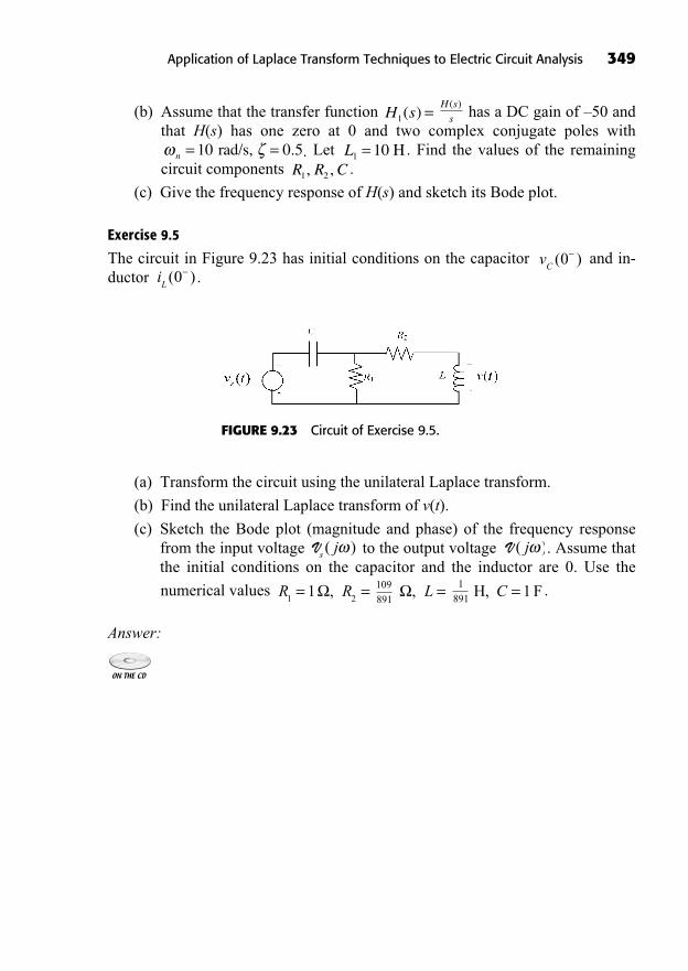
(b) Assume that the transfer function has a DC gain of –50 andthat H(s) has one zero at 0 and two complex conjugate poles with
. Let . Find the values of the remainingcircuit components .
(c) Give the frequency response of H(s) and sketch its Bode plot.
Exercise 9.5
The circuit in Figure 9.23 has initial conditions on the capacitor and in-ductor .i
L( )0
vC
( )0
R R C1 2, ,L1 10= Hn = =10 0 5 rad/s, .
H s
s
( )H s1( ) =
Application of Laplace Transform Techniques to Electric Circuit Analysis 349
FIGURE 9.23 Circuit of Exercise 9.5.
(a) Transform the circuit using the unilateral Laplace transform.
(b) Find the unilateral Laplace transform of v(t).
(c) Sketch the Bode plot (magnitude and phase) of the frequency responsefrom the input voltage to the output voltage . Assume thatthe initial conditions on the capacitor and the inductor are 0. Use the
numerical values .
Answer:
C 1=H, F1
891L =,109
891R R
1 21= =,
V ( )jVs
j( )

This page intentionally left blank
351
State Models ofContinuous-TimeLTI Systems
10
((Lecture 33: State Models of Continuous-Time LTI Systems))
In Chapter 3 we studied an important class of continuous-time linear time-invariant (LTI) systems defined by linear, causal constant-coefficient differen-tial equations. For a system described by an Nth-order differential equation, it is
always possible to find a set of N first-order differential equations and an outputequation describing the same input-output relationship. These N first-order differ-ential equations are called the state equations of the system. The states are the Nvariables seen as outputs of the state equations.
The concept of state is directly applicable to certain types of engineering sys-tems such as linear circuits and mechanical systems. The state variables in a circuit
In This Chapter
State Models of Continuous-Time LTI Differential SystemsZero-State Response and Zero-Input Response of a Continuous-TimeState-Space SystemLaplace-Transform Solution for Continuous-Time State-Space SystemsState Trajectories and the Phase PlaneBlock Diagram Representation of Continuous-Time State-Space SystemsSummaryTo Probe FurtherExercises
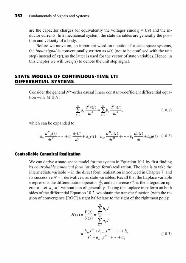
352 Fundamentals of Signals and Systems
are the capacitor charges (or equivalently the voltages since q = Cv) and the in-ductor currents. In a mechanical system, the state variables are generally the posi-tion and velocity of a body.
Before we move on, an important word on notation: for state-space systems,the input signal is conventionally written as u(t) (not to be confused with the unitstep) instead of x(t), as the latter is used for the vector of state variables. Hence, inthis chapter we will use q(t) to denote the unit step signal.
STATE MODELS OF CONTINUOUS-TIME LTI DIFFERENTIAL SYSTEMS
Consider the general Nth-order causal linear constant-coefficient differential equa-tion with :
(10.1)
which can be expanded to
(10.2)
Controllable Canonical Realization
We can derive a state-space model for the system in Equation 10.1 by first findingits controllable canonical form (or direct form) realization. The idea is to take theintermediate variable w in the direct form realization introduced in Chapter 7, andits successive N – 1 derivatives, as state variables. Recall that the Laplace variables represents the differentiation operator , and its inverse s–1 is the integration op-erator. Let without loss of generality. Taking the Laplace transform on bothsides of the differential Equation 10.2, we obtain the transfer function (with the re-gion of convergence [ROC] a right half-plane to the right of the rightmost pole):
(10.3)
H sY s
U s
b s
a s
b s b s
kk
k
M
kk
k
N
MM
M
( )( )
( )= =
=+
=
=
0
0
1MM
NN
N
b
s a s a
+ ++ + +
10
11
0
.
aN = 1
d
dt
ad y t
dtady t
dta y t b
d u t
dtN
N
N M
M
M
( ) ( )( )
( )+ + + = + 1 0 + +b
du t
dtb u t1 0
( )( ).
ad y t
dtbd u t
dtk
k
kk
N
k
k
kk
M( ) ( ),
= =
=0 0
M N
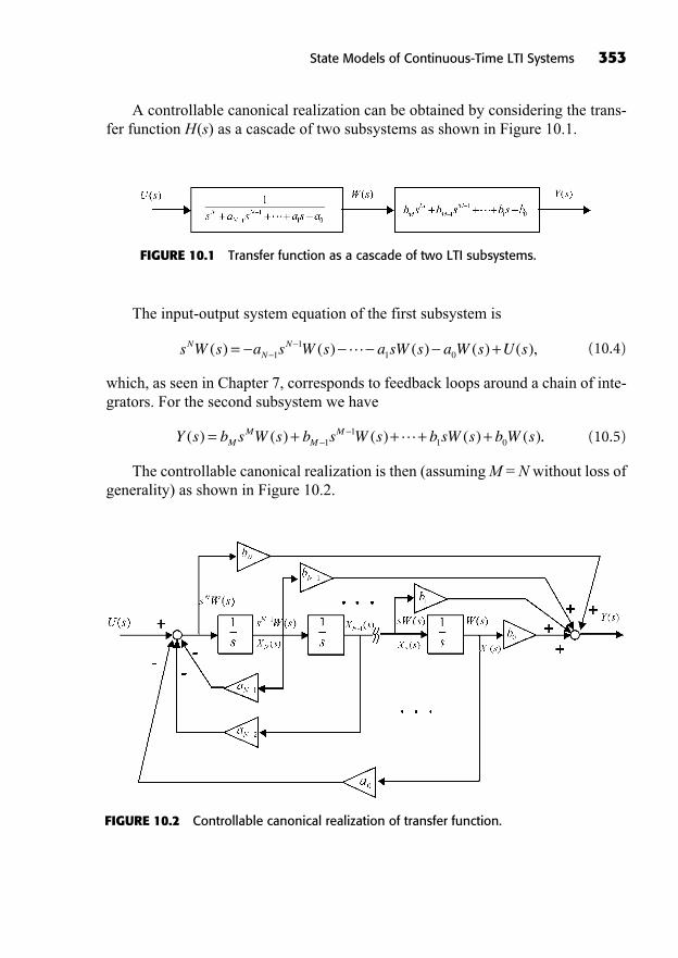
State Models of Continuous-Time LTI Systems 353
A controllable canonical realization can be obtained by considering the trans-fer function H(s) as a cascade of two subsystems as shown in Figure 10.1.
FIGURE 10.1 Transfer function as a cascade of two LTI subsystems.
The input-output system equation of the first subsystem is
(10.4)
which, as seen in Chapter 7, corresponds to feedback loops around a chain of inte-grators. For the second subsystem we have
(10.5)
The controllable canonical realization is then (assuming M = N without loss ofgenerality) as shown in Figure 10.2.
Y s b s W s b s W s b sW s b W sMM
MM( ) ( ) ( ) ( ) ( )= + + + +1
11 0 ..
s W s a s W s a sW s a W s U sNN
N( ) ( ) ( ) ( ) ( ),= +11
1 0
FIGURE 10.2 Controllable canonical realization of transfer function.
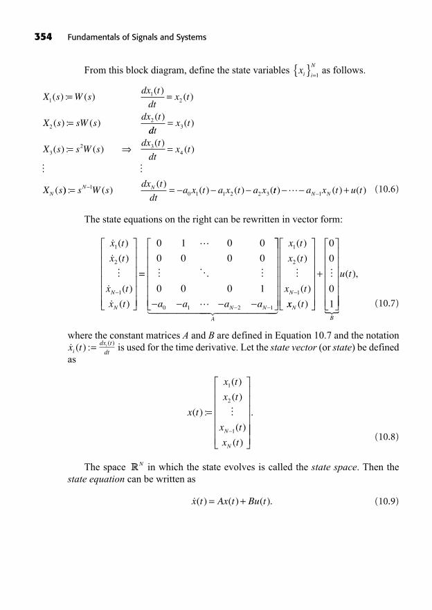
354 Fundamentals of Signals and Systems
From this block diagram, define the state variables as follows.
(10.6)
The state equations on the right can be rewritten in vector form:
(10.7)
where the constant matrices A and B are defined in Equation 10.7 and the notationis used for the time derivative. Let the state vector (or state) be defined
as
(10.8)
The space in which the state evolves is called the state space. Then thestate equation can be written as
(10.9)�x t Ax t Bu t( ) ( ) ( ).= +
RN
x t
x t
x t
x t
x tN
N
( ) :
( )
( )
( )
( )
=
1
2
1
� .
dx t
dti ( )�x ti ( ) :=
��
���
x t
x t
x t
x tN
N
1
2
1
( )
( )
( )
( )
==
0 1 0 0
0 0 0 0
0 0 0 1
0 1 2 1
� � �
a a a aN N
A
N
x t
x t
x t
� ������� �������
�
1
2
1
( )
( )
( )
xx tN ( )
+
0
0
0
1
�
B
u t
�
( ),
X s W sdx t
dtx t
X s sW sdx t
11
2
22
( ) : ( )( )
( )
( ) : ( )( )
= =
=ddt
x t
X s s W sdx t
dtx t
X sN
=
= =
3
32 3
4
( )
( ) : ( )( )
( )
(
� �
)) : ( )( )
( ) ( ) (= =s W sdx t
dta x t a x t a xN N1
0 1 1 2 2 3 tt a x t u tN N) ( ) ( )+ 1
xi i
N{ } =1
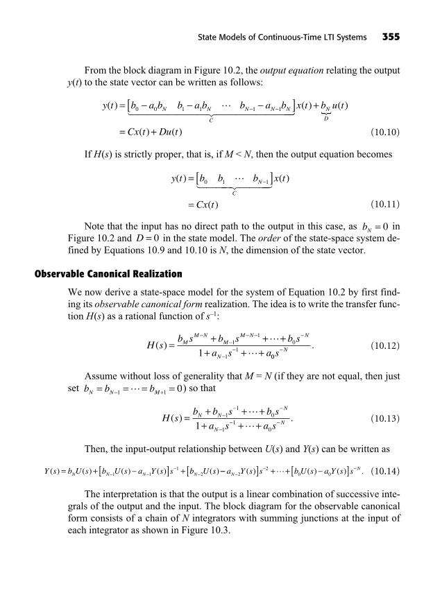
From the block diagram in Figure 10.2, the output equation relating the outputy(t) to the state vector can be written as follows:
(10.10)
If H(s) is strictly proper, that is, if M < N, then the output equation becomes
(10.11)
Note that the input has no direct path to the output in this case, as inFigure 10.2 and in the state model. The order of the state-space system de-fined by Equations 10.9 and 10.10 is N, the dimension of the state vector.
Observable Canonical Realization
We now derive a state-space model for the system of Equation 10.2 by first find-ing its observable canonical form realization. The idea is to write the transfer func-tion H(s) as a rational function of s–1:
(10.12)
Assume without loss of generality that M = N (if they are not equal, then justset ) so that
(10.13)
Then, the input-output relationship between U(s) and Y(s) can be written as
(10.14)
The interpretation is that the output is a linear combination of successive inte-grals of the output and the input. The block diagram for the observable canonicalform consists of a chain of N integrators with summing junctions at the input ofeach integrator as shown in Figure 10.3.
Y s b U s b U s a Y s s b U sN N N N( ) ( ) ( ) ( ) ( )= + [ ] +1 11
2[ ] + + [ ]a Y s s b U s a Y s sNN
22
0 0( ) ( ) ( ) .
H sb b s b s
a s a sN N
N
NN( ) .=
+ + ++ + +
11
0
11
01
b b bN N M= = = =+1 1 0
H sb s b s b s
a s aM
M NM
M N N
N
( ) =+ + +
+ + +1
10
111
00s
N .
D = 0bN = 0
y t b b b x t
Cx t
N
C
( ) ( )
( )
= [ ]
=
0 1 1� ���� ����
y t b a b b a b b a bN N N N N
C
( ) = [ ]0 0 1 1 1 1� �������� ��������� �x t b u t
Cx t Du t
N
D
( ) ( )
( ) ( )
+
= +
State Models of Continuous-Time LTI Systems 355
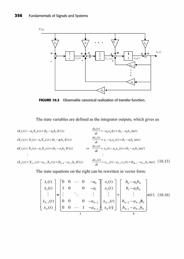
356 Fundamentals of Signals and Systems
The state variables are defined as the integrator outputs, which gives us
(10.15)
The state equations on the right can be rewritten in vector form:
(10.16)
��
���
x t
x t
x t
x tN
N
1
2
1
( )
( )
( )
( )
==
0 0 0
1 0 0
0 0 0
0 0 1
0
1
2
1
� � �
a
a
a
aN
N
A
N
N
x t
x t
x t
x t� ����� �����
�
1
2
1
( )
( )
( )
( ))
+
b a b
b a b
b a
N
N
N N
0 0
1 1
2 2
�bb
b a b
u t
N
N N N
B
1 1� ��� ���
( ).
sX s a X s b a b U sdx t
dta xN N N1 0 0 0
10( ) ( ) ( ) ( )
( )= + = (( ) ( ) ( )
( ) ( ) ( ) (
t b a b u t
sX s X s a X s b
N
N
+
= +
0 0
2 1 1 1 aa b U sdx t
dtx a x t b a b u tN N N1
21 1 1 1) ( )
( )( ) ( ) ( )= +
ssX s X s a X s b a b U sdx t
dN N3 2 2 2 23( ) ( ) ( ) ( ) ( )( )
= +tt
x t a x t b a b u tN N= +2 2 2 2( ) ( ) ( ) ( )
� �
sX s X s a X s bN N N N N( ) ( ) ( ) (= +1 1 11 1 1 1= +a b U sdx t
dtx t a x t bN N
NN N N) ( )
( )( ) ( ) ( NN N Na b u t1 1 ) ( )
FIGURE 10.3 Observable canonical realization of transfer function.
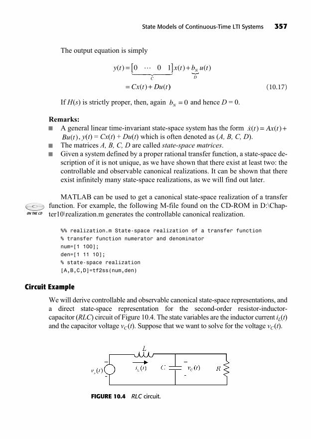
The output equation is simply
(10.17)
If H(s) is strictly proper, then, again and hence D = 0.
Remarks:A general linear time-invariant state-space system has the form
, y(t) = Cx(t) + Du(t) which is often denoted as (A, B, C, D). The matrices A, B, C, D are called state-space matrices.Given a system defined by a proper rational transfer function, a state-space de-scription of it is not unique, as we have shown that there exist at least two: thecontrollable and observable canonical realizations. It can be shown that thereexist infinitely many state-space realizations, as we will find out later.
MATLAB can be used to get a canonical state-space realization of a transferfunction. For example, the following M-file found on the CD-ROM in D:\Chap-ter10\realization.m generates the controllable canonical realization.
%% realization.m State-space realization of a transfer function
% transfer function numerator and denominator
num=[1 100];
den=[1 11 10];
% state-space realization
[A,B,C,D]=tf2ss(num,den)
Circuit Example
We will derive controllable and observable canonical state-space representations, anda direct state-space representation for the second-order resistor-inductor-capacitor (RLC) circuit of Figure 10.4. The state variables are the inductor current iL(t)and the capacitor voltage vC(t). Suppose that we want to solve for the voltage vC(t).
Bu t( )�x t Ax t( ) ( )= +
bN = 0
y t x t b u t
Cx t Du tC
N
D
( ) ( ) ( )
( ) (
= [ ] +
= +
0 0 1� ��� ��� �
))
State Models of Continuous-Time LTI Systems 357
FIGURE 10.4 RLC circuit.
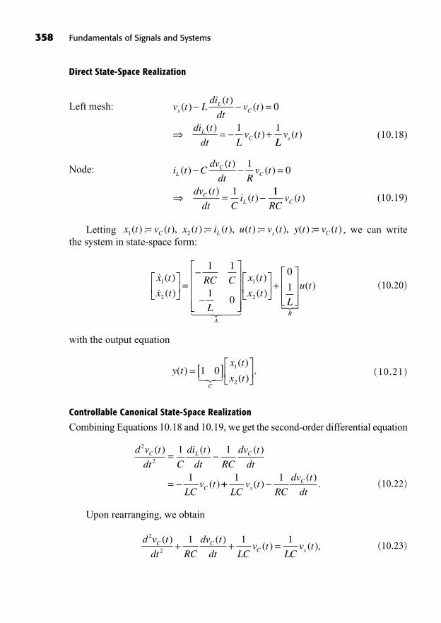
358 Fundamentals of Signals and Systems
Direct State-Space Realization
Left mesh:
(10.18)
Node:
(10.19)
Letting , we can writethe system in state-space form:
(10.20)
with the output equation
(10.21)
Controllable Canonical State-Space Realization
Combining Equations 10.18 and 10.19, we get the second-order differential equation
(10.22)
Upon rearranging, we obtain
(10.23)d v t
dt RC
dv t
dt LCv t
LCv tC C
C s
2
2
1 1 1( ) ( )( ) ( ),+ + =
d v t
dt C
di t
dt RC
dv t
dt
LCv t
C L C
C
2
2
1 1
1
( ) ( ) ( )
( )
=
= ++1 1
LCv t
RC
dv t
dtsC( )
( ).
y tx t
x tC
( )( )
( ).= [ ]1 0 1
2���
��
�
x t
x tRC C
LA
1
2
1 1
10
( )
( )=
��� ���
x t
x tL
u t
B
1
2
0
1( )
( )( )+
x t v t x t i t u t v t y tC L s1 2( ) : ( ), ( ) : ( ), ( ) : ( ), ( ) := = = == v tC ( )
i t Cdv t
dt Rv t
dv t
dt Ci t
LC
C
CL
( )( )
( )
( )( )
=
=
10
1 11
RCv tC ( )
v t Ldi t
dtv t
di t
dt Lv t
sL
C
LC
( )( )
( )
( )( )
=
= +
0
1 1
LLv ts ( )
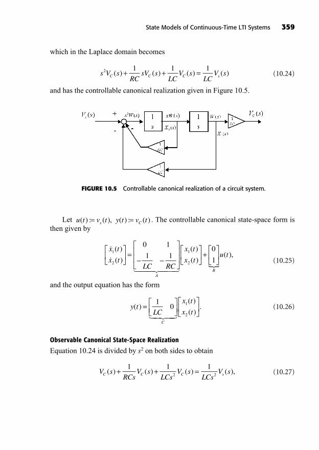
State Models of Continuous-Time LTI Systems 359
which in the Laplace domain becomes
(10.24)
and has the controllable canonical realization given in Figure 10.5.
s V sRC
sV sLC
V sLC
V sC C C s2 1 1 1
( ) ( ) ( ) ( )+ + =
FIGURE 10.5 Controllable canonical realization of a circuit system.
Let . The controllable canonical state-space form isthen given by
(10.25)
and the output equation has the form
(10.26)
Observable Canonical State-Space Realization
Equation 10.24 is divided by s2 on both sides to obtain
(10.27)V sRCs
V sLCs
V sLCs
V sC C C s( ) ( ) ( ) ( ),+ + =1 1 1
2 2
y tLC
x t
x tC
( )( )
( ).=
10 1
2� �� ��
��
� ��� �
x t
x tLC RC
A
1
2
0 1
1 1( )
( )=
����
x t
x tu t
B
1
2
0
1
( )
( )( ),+
u t v t y t v ts C( ) : ( ), ( ) : ( )= =

360 Fundamentals of Signals and Systems
which is rewritten as
(10.28)
This equation is represented by the block diagram in Figure 10.6.
V sRCs
V ss LC
V sLC
V sC C s C( ) ( ) ( ) ( )= +1 1 1 1
2 ..
FIGURE 10.6 Observable canonical realization of a circuit system.
Let . The observable canonical state-space realiza-tion is given by
(10.29)
and the output equation is simply
(10.30)y tx t
x tC
( )( )
( ).= [ ]0 1 1
2���
��
�
x t
x tLC
RCA
1
2
01
11
( )
( )=
��� ���
x t
x tLC u t
B
1
2
1
0
( )
( )( ),+
u t v t y t v ts C( ) : ( ), ( ) : ( )= =

((Lecture 34: Zero-State Response and Zero-Input Response))
ZERO-STATE RESPONSE AND ZERO-INPUT RESPONSE OF ACONTINUOUS-TIME STATE-SPACE SYSTEM
Recall that the response of a system with nonzero initial conditions is composed ofa zero-state response due to the input signal only and a zero-input response due tothe initial conditions only. For a state-space system, the initial conditions are cap-tured in the initial state x(0).
Zero-Input Response
Consider the following general continuous-time, single-input, single-output, Nth-order LTI state-space system:
(10.31)
where , and .The zero-input response is the response to an initial state only.The state equation is then
(10.32)
The solution to this homogeneous state equation involves the matrix exponen-tial function, which is defined as a power series of a square matrix :
(10.33)
where is the identity matrix. It can be shown that this power series con-verges for any matrix A. Note that this definition generalizes the definition of thescalar exponential function . How do we compute ? One way is todiagonalize the matrix A and take the exponential of the eigenvalues. Specifically,if matrix diagonalizes A, that is,
(10.34):= =
1
2 1
0 0
0 0
0 0
� � � N
T AT
T N N×C
eAe aa , R
N N×IN
e I A A AkAA
Nk:
! !,= + + + + + +
1
2
1
3
12 3
A N N×R
�x t Ax t( ) ( ).=
x x( )0 0=y tzi ( )A B C DN N N N× × ×R R R R, , ,1 1x t y t u tN( ) , ( ) , ( )R R R
�x t Ax t Bu t
y t Cx t Du t
( ) ( ) ( )
( ) ( ) ( ),
= += +
State Models of Continuous-Time LTI Systems 361
where is the eigenvalue (all eigenvalues are assumed to be distinct) ofthe matrix A, then the exponential of A is given by
(10.35)
The matrix of eigenvectors of A is diagonalizing, so we can use it as matrix T.The time-dependent matrix exponential is simply
(10.36)
Now consider the vector-valued function of time
(10.37)
where and . The claim is that this function is the state responseof the system to the initial state for . To show this, simply substitute Equation10.37 into the left-hand side of Equation 10.32:
(10.38)
dx t
dt
d
dte x
d
dtI At A t xAtn
( )= = + + +
=
02 2
0
1
2
AA A t A t x
A I At A tn
+ + +
= + + +
2 3 20
2 2
1
2
1
2
= =
x
Ae x Ax tAt
0
0 ( )
t > 0x x( )0 0=x t N( ) R
x t e xAt( ) ,= 0
e e T
e
e
e
At T T t
t
t
tN
= =1
1
2
0 0
0
0
0 0
�
� �
T 1.
eAt
e e I T T T T T Tk
A T TN= = + + + + +
1 1 2 1 3 11
2
1
3
1
! ! TT T
T Ik
T
k
Nk
+
= + + + + + +
1
2 31
2
1
3
1
! !
=
=
1
1
1
2
0 0
0
0
0 0
Te T
T
e
e
e N
�
� �
T 1
ithi C
362 Fundamentals of Signals and Systems
Therefore, the zero-input state response is as given in Equation 10.37 for ,and the corresponding zero-input response is
(10.39)
where q(t) is the unit step signal.
Example 10.1: Let us revisit the circuit example with its first physically moti-vated state-space representation:
(10.40)
(10.41)
Suppose , the initial capacitor voltage is x1(0) = 10 V,and the initial inductor current is x2(0) = 0 A. With these numerical values, the stateequation becomes
(10.42)
We want to find the zero-input state response of the circuit. We first computethe eigenvalues of A:
(10.43)
det( ) det
,
I A2
2
1 2
1 1
10
1 0
=+
=
+ + =
= ±1
2
3
2j .
��
��� ��
x
x
x
xA
1
2
1
2
1 1
1 0
0= +
11B
sv�
.
R L C= = =1 1 1, ,H F
y tx t
x t( )
( )
( ).= [ ]1 0 1
2
��
�
x t
x tRC C
LA
1
2
1 1
10
( )
( )=
��� ���
x t
x tL
u t
B
1
2
0
1( )
( )( ),+
y t Ce x q tziAt( ) ( ),= 0
t > 0
State Models of Continuous-Time LTI Systems 363
Then, the corresponding eigenvectors are computed:
(10.44)
Letting
(10.45)
and
(10.46)
we check that :T T A=1
: ,=+
1
2
3
20
01
2
3
2
j
j
T v vj j
:= [ ] = +1 2
1
2
3
2
1
2
3
21 1
( )1 2 1
11
0
1
2
3
21
11
2
3
2
I A v
j
j
v
=
+
+vv
v
vj
12
11
12
0
0
1
2
3
21
=
=
=( )2 2 2 0
1
2
3
21
11
2
3
2
I A v
j
j
=
=
v
v
v
v
21
22
21
22
0
0
1
2++ j
3
21
.
v v1 2,
364 Fundamentals of Signals and Systems
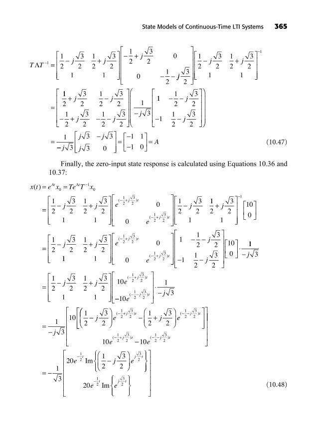
(10.47)
Finally, the zero-input state response is calculated using Equations 10.36 and10.37:
(10.48)
x t e x Te T x
j j
At t( ) = =
= +
01
0
1
2
3
2
1
2
3
21 1
+
+
e
e
jj t
j t
( )
( )
12
32
12
32
0
0
1
2
3
2
11
2
3
21 1
10
0
1
2
3
2
1
2
3
2
1
+
= +
j
j j
11 1
0
0
12
32
12
32
+
+
e
e
j t
j t
( )
( )
11
2
3
2
11
2
3
2
10
0
j
j
11
3
1
2
3
2
1
2
3
21 1
1012
32
= ++
j
j j ej t( )
=
10
1
3
1
3
101
2
3
2
12
32e
j
j
j
j t( )
++
e j ej t j t( ) ( )
12
32
12
32
1
2
3
2
+10 10
12
32
12
32e e
j t j t( ) ( )
=1
3
201
2
3
2
12
32e j e
t j tIm
2012
32e e
t j tIm
T Tj j
j= +
+1
1
2
3
2
1
2
3
21 1
1
2
3
20
01
2jj
j j
3
2
1
2
3
2
1
2
3
21 1
1
+
=
11
2
3
2
1
2
3
2
1
2
3
2
1
2
3
2
1
3
+
+
j j
j jj
111
2
3
2
11
2
3
2
1=
j
j
= =j
j j
jA
3
3 3
3 0
1 1
1 0
State Models of Continuous-Time LTI Systems 365
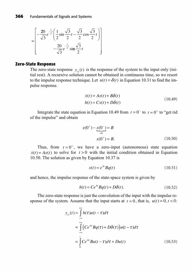
Zero-State ResponseThe zero-state response is the response of the system to the input only (ini-tial rest). A recursive solution cannot be obtained in continuous time, so we resortto the impulse response technique. Let in Equation 10.31 to find the im-pulse response.
(10.49)
Integrate the state equation in Equation 10.49 from to to “get ridof the impulse” and obtain
(10.50)
Thus, from , we have a zero-input (autonomous) state equationto solve for with the initial condition obtained in Equation
10.50. The solution as given by Equation 10.37 is
(10.51)
and hence, the impulse response of the state-space system is given by
(10.52)
The zero-state response is just the convolution of the input with the impulse re-sponse of the system. Assume that the input starts at , that is, :
(10.53)
y t h u t d
Ce Bq D u
zs
A
( ) ( ) ( )
( ) ( )
=
= +( )
+
(( )
( ) ( )
t d
Ce Bu t d Du tAt
= +
+
0
u t t( ) ,= <0 0t = 0
h t Ce Bq t D tAt( ) ( ) ( ).= +
x t e Bq tAt( ) ( )=
t > 0�x t Ax t( ) ( )=t = +0
x x B
x B
( ) ( )
( ) .
0 0
00
+
=+
=
=
�
t = +0t = 0
�x t Ax t B t
h t Cx t D t
( ) ( ) ( )
( ) ( ) ( )
= += +
u t t( ) ( )=
y tzs ( )
=
220
3
1
2
3
2
3
2
3
2
20
3
12
12
e t t
e
t
t
sin cos
sinn3
2t
366 Fundamentals of Signals and Systems
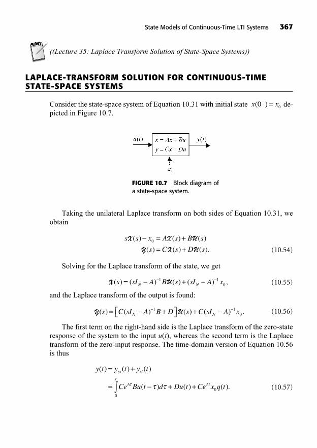
State Models of Continuous-Time LTI Systems 367
((Lecture 35: Laplace Transform Solution of State-Space Systems))
LAPLACE-TRANSFORM SOLUTION FOR CONTINUOUS-TIMESTATE-SPACE SYSTEMS
Consider the state-space system of Equation 10.31 with initial state de-picted in Figure 10.7.
x x( )0 0=
FIGURE 10.7 Block diagram ofa state-space system.
Taking the unilateral Laplace transform on both sides of Equation 10.31, weobtain
(10.54)
Solving for the Laplace transform of the state, we get
(10.55)
and the Laplace transform of the output is found:
(10.56)
The first term on the right-hand side is the Laplace transform of the zero-stateresponse of the system to the input u(t), whereas the second term is the Laplacetransform of the zero-input response. The time-domain version of Equation 10.56is thus
(10.57)
y t y t y t
Ce Bu t d Du t C
zs zi
At
( ) ( ) ( )
( ) ( )
= +
= + +0
ee x q tAt0 ( ).
Y U( ) ( ) ( ) ( ) .s C sI A B D s C sI A xN N= + +1 10
X U( ) ( ) ( ) ( ) ,s sI A B s sI A xN N= +1 10
s s x A s B s
s C s D s
X X UY X U
( ) ( ) ( )
( ) ( ) ( ).
= += +
0
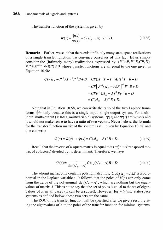
The transfer function of the system is given by
(10.58)
Remark: Earlier, we said that there exist infinitely many state-space realizationsof a single transfer function. To convince ourselves of this fact, let us simply consider the (infinitely many) realizations expressed by
whose transfer functions are all equal to the one given inEquation 10.58:
Note that in Equation 10.58, we can write the ratio of the two Laplace trans-forms only because this is a single-input, single-output system. For multi-input, multi-output (MIMO, multivariable) systems, and U(s) are vectors andit would not make sense to have a ratio of two vectors. Nevertheless, the formulafor the transfer function matrix of the system is still given by Equation 10.58, andone can write
(10.59)
Recall that the inverse of a square matrix is equal to its adjoint (transposed ma-trix of cofactors) divided by its determinant. Therefore, we have
(10.60)
The adjoint matrix only contains polynomials; thus, is a poly-nomial in the Laplace variable s. It follows that the poles of H(s) can only comefrom the zeros of the polynomial , which are nothing but the eigen-values of matrix A. This is not to say that the set of poles is equal to the set of eigen-values of A in all cases (it can be a subset). However, for minimal state-spacesystems as defined below, these two sets are the same.
The ROC of the transfer function will be specified after we give a result relat-ing the eigenvalues of A to the poles of the transfer function for minimal systems.
det( )sI AN
C sI A BNadj( )
H ( )det( )
( ) .ssI A
C sI A B DN
N= +1
adj
H U Y( ) ( ) ( ) ( ) .s s s C sI A B DN= = +� 1
Y( )s
YU
( )
( )
s
s
CP sI P AP P B D CP sP P P AP P BN( ) ( )+ =1 1 1 1 1 1 1 ++
= +
=
D
CP P sI A P P B D
CPP sI A
N
N
1 1 1
1
( )
( ) 11 1
1
PP B D
C sI A B DN
+
= +( ) .
, det( )P PN N× 0R( , , , ),P AP P B CP D1 1
HYU
( )( )
( )( ) .s
s
sC sI A B DN= = +1
368 Fundamentals of Signals and Systems
Bounded-Input, Bounded-Output Stability
Minimal state-space realizations are realizations for which all N eigenvalues of ma-trix A appear as poles in the transfer function given by Equation 10.58 with theirmultiplicity. In other words, minimal state-space realizations are those realizationsfor which the order of the transfer function is the same as the dimension of the statevector.
Fact: For a minimal state-space realization (A, B, C, D) of a continuous-timesystem with transfer function H(s), the set of poles of H(s) is equal to the set ofeigenvalues of A.
Since we limit our analysis to causal, minimal state-space realizations, this fact yields the following stability theorem for such continuous-time, LTI state-space systems.
Stability Theorem: The continuous-time causal, minimal, LTI state-space sys-tem (A, B, C, D), where , is bounded-input,bounded-output (BIBO) stable if and only if all eigenvalues of A have a negativereal part.
Mathematically, (A, B, C, D) is BIBO stable if and only if .
The ROC of the transfer function in Equation 10.58 is the open right half-planeto the right of .
We found earlier that the impulse response of the state-space system is givenby , where q(t) is the unit step function. Comparing this expression with Equation 10.58, the inverse Laplace transform of
is found to be equal to ; that is,
(10.61)
Example 10.2: Find the transfer function of the causal minimal state-space sys-tem described by
(10.62)
First, we compute the eigenvalues of the A matrix by solving to obtain . Thus, the system is BIBO stable since the poles of thetransfer function are negative, being equal to the eigenvalues. We use Equation10.58 to calculate H(s):
1 21 2= =,det I A( ) = 0
�x t x t u( ). .
. .( ) (= +
2 2 0 4
0 6 0 8
2
1tt
y t x t u t
)
( ) ( ) ( ).= [ ] +1 3 2
e q t sI A s AAt UL
Ni N
i( ) ( ) , Re max Re ( ), ,
{ } >=
1
1…{{ }
e q tAt ( )( ) , Re max Re ( ), ,
sI A s ANi N
i{ } > { }=
1
1…
h t Ce Bq t D tAt( ) ( ) ( )= +
max Re ( ), ,i N
i A={ }
1…
, ,i N= 1…Re ( ) ,i A{ } < 0
A B C DN N N N× × ×R R R R, , ,1 1
State Models of Continuous-Time LTI Systems 369
(10.63)
The eigenvalues of the A matrix are the same as the poles of the transfer func-tion, as expected since the realization is minimal. Now that the transfer function isknown, the output response of the system for a specific input can be found by theusual method of partial fraction expansion of Y(s) = H(s)U(s).
STATE TRAJECTORIES AND THE PHASE PLANE
The time evolution of an N-dimensional state vector x(t) can be depicted using Nplots of the state variables versus time. On the other hand, the state trajectory,that is, the locus of points traced by x(t), is a curved line in hyperspace .
For a two-dimensional state vector, we can conveniently plot the state trajec-tory on a phase plane that is a plot of x2(t) versus x1(t) (or vice versa). For exam-ple, the state trajectory in the phase plane of a second-order system responding toan initial vector as a damped sinusoid will look like a spiral encircling and goingtoward the origin.
Example 10.3: Consider the causal second-order mass-spring-damper system ofFigure 10.8 modeled as a state-space system.
Assume that the mass-spring-damper system is initially at rest, which meansthat the spring generates a force equal to the force of gravity to support the mass.The balance of forces on the mass and Newton’s law gives us an equation for statevariable x2(t):
(10.64)
and the second equation simply relates velocity and position:
(10.65)�x t x t1 2( ) ( ).=
mx t u t F t F t
u t kx t bx tk b�2
1 2
( ) ( ) ( ) ( )
( ) ( ) ( )
== ,,
�Nx ti ( )
H ss
s( )
. .
. .= [ ] +
+1 3
2 2 0 4
0 6 0 8
2
1
1
+
=+ +
[ ] +
2
1
2 2 0 8 0 4 0 61 3
0 8 0
( . )( . ) ( . ) .
. .
s s
s 44
0 6 2 2
2
12
1
3 21 3
22
++
=+ +
[ ]
. .s
s s
ss
s
s s s
s
++ =
+ + ++
1 2
3 42
5 11 4 2 3 22
2
.
.. ( )
33 2
2 7 4
3 22
0 5 3 7
3 2
2
2
2
2
s
s s
s s
s s
s s
+
=++ +
=++ +
=. . .
222 19 1 69
1 21
( . )( . )
( )( ), Re{ }
s s
s ss
++ +
>
370 Fundamentals of Signals and Systems
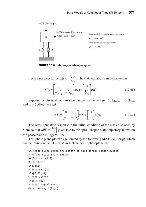
State Models of Continuous-Time LTI Systems 371
Let the state vector be . The state equation can be written as
(10.66)
Suppose the physical constants have numerical values , ,and . We get
(10.67)
The zero-input state response to the initial condition of the mass displaced by
5 cm so that gives rise to the spiral-shaped state trajectory shown on
the phase plane in Figure 10.9.This phase plane plot was generated by the following MATLAB script, which
can be found on the CD-ROM in D:\Chapter10\phaseplane.m.
%% Phase plane state trajectory of mass-spring-damper system
% Define state-space system
A=[0 1; -1 -0.5];
B=[0; 0.1];
C=eye(2);
D=zeros(2,1);
x0=[0.05; 0];
% time vector
T=0:.1:100;
% input signal (zero)
U=zeros(length(T),1);
.0 05
0x( )0 =
�x t x t u t( ).
( ).
( ).= +0 1
1 0 5
0
0 1
b = 5 N ms
k = 10 N mm = 10 kg
�x t km
bm
x tm
u t( ) ( ) ( ).= +0 1 0
1
x t
x t
( )
( )1
2
x t( ) :=
FIGURE 10.8 Mass-spring-damper system.
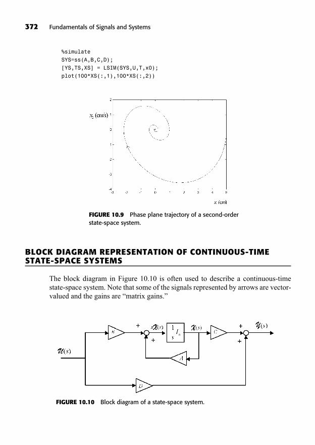
372 Fundamentals of Signals and Systems
%simulate
SYS=ss(A,B,C,D);
[YS,TS,XS] = LSIM(SYS,U,T,x0);
plot(100*XS(:,1),100*XS(:,2))
FIGURE 10.9 Phase plane trajectory of a second-orderstate-space system.
BLOCK DIAGRAM REPRESENTATION OF CONTINUOUS-TIMESTATE-SPACE SYSTEMS
The block diagram in Figure 10.10 is often used to describe a continuous-timestate-space system. Note that some of the signals represented by arrows are vector-valued and the gains are “matrix gains.”
FIGURE 10.10 Block diagram of a state-space system.

One can see that this is a generalization of a scalar first-order system, with Nintegrators in parallel instead of just one. Remember that matrices do not commutein general, even if they are conformable. Thus, in deriving the equations for the above block diagram, one has to be careful not to write something like
. In other words, the order inwhich subsystems appear in block diagrams of multivariable LTI systems cannotbe changed.
SUMMARY
In this chapter, we introduced LTI state-space systems.
A state model of a physical system can often be obtained from first principlesas a collection of first-order differential equations together with an outputequation.Two state-space realizations of any proper rational transfer function can be eas-ily obtained: the controllable canonical realization and the observable canoni-cal realization. However, there exist infinitely many realizations of any givenproper rational transfer function.We derived the formulas for the zero-input and zero-state responses, the im-pulse response, and the transfer function of a general LTI state-space system.A causal minimal state-space system was shown to be BIBO stable if and onlyif all of the eigenvalues of its A matrix lie in the open left half-plane.We briefly discussed state trajectories, and the phase plane was illustrated withan example.
TO PROBE FURTHER
State-space modeling of engineering systems is covered in Bélanger, 1995. For anadvanced text on state-space systems, see Chen, 1999.
EXERCISES
Exercises with Solutions
Exercise 10.1
Consider the causal LTI state-space system:
C sI A B B sI A C CB sI AN N N( ) ( ) ( )= =1 1 1
State Models of Continuous-Time LTI Systems 373
where .
(a) Is the system stable? Justify your answer.
Answer:We compute the eigenvalues of the A matrix:
The eigenvalues of the A matrix have a negative real part; there-fore the system is stable.
(b) Compute the transfer function H(s) of the system. Specify its ROC.
Answer:
The poles of the transfer function are , equal to the eigenvalues, as expected.
(c) Compute the impulse response h(t) of the system using the matrix exponential.
Answer:The eigenvectors of the A matrix are computed as follows:
= ± j1 1
1
2± j2 2
1
2± =n nj 1 2
H s C sI A B
s
s
( ) ( )=
= [ ] ++
21
1
1 11 1
1 1
1
0
=+ +
[ ] ++
=
1
2 21 1
1 1
1 1
1
0
1
2s s
s
s
s22 22 21 1
1
1 2 21
+ +[ ] +
=+ +
>s
s s
s ss, Re{ }
1 2 1, = ± j
det ( )( )+
+= + + + = + +
=
1 1
1 11 1 1 2 22
1 + =1 12j j, ,
C = [ ]1 1,1
0B =,1 1
1 1A =
�x Ax Bu
y Cx
= += ,
374 Fundamentals of Signals and Systems
Thus, , and
Thus, .
Exercise 10.2
Find the controllable and observable canonical state-space realizations for the fol-lowing LTI system:
H ss s
s ss( ) , Re{ } .=
+ ++
>3
3
2
30
h t e t t q tt( ) cos sin ( )= ( )
h t CT e e T q tj t j t( ) { , } ( )( ) ( )=
= [ ]
+diag 1 1 1
1 11 11 0
0
1
2
1
21
2
1
1j j
e
e
jj t
j t
+( )
( )
jj
q t
j je j
1
2
1
0
1 11
= +[ ]+
( )
( ))
( )( )
t
j teq t
0
0
1
21
2
1
2
1
= + jj e j ej t j t1
2
1
2
1
21 1++( ) ( )
= + +
q t
e j e j et jt jt
( )
1
2
1
2
1
2
1
2
= +
q t
e j e q tt jt
( )
Re ( )21
2
1
2== ( )e t t q tt cos sin ( ),
Tj j
Tj
j
j
j= = =
1 1 1
2
1
1
1
2
1
21
1,
22
1
2j
( )1 111
12
1 1 1
1 1 1I A v
j
j
v
v=
+ ++ +
== =
=
j
j
v
v
v v
1
1
0
0
1
11
12
11 1, 22
2 1
1
=
= =
j
v vj
State Models of Continuous-Time LTI Systems 375
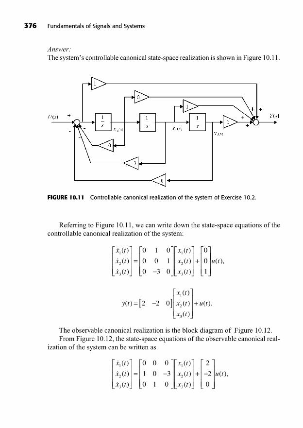
376 Fundamentals of Signals and Systems
Answer:The system’s controllable canonical state-space realization is shown in Figure 10.11.
FIGURE 10.11 Controllable canonical realization of the system of Exercise 10.2.
Referring to Figure 10.11, we can write down the state-space equations of thecontrollable canonical realization of the system:
The observable canonical realization is the block diagram of Figure 10.12.From Figure 10.12, the state-space equations of the observable canonical real-
ization of the system can be written as
���
x t
x t
x t
1
2
3
0 0 0
1 0 3
0 1 0
( )
( )
( )
= +x t
x t
x t
1
2
3
2
2
0
( )
( )
( )
u t( ),
y t
x t
x t
x t
u t( )
( )
( )
( )
( ).= [ ] +2 2 01
2
3
���
x t
x t
x t
1
2
3
0 1 0
0 0 1
0 3 0
( )
( )
( )
= +x t
x t
x t
1
2
3
0
0
1
( )
( )
( )
u t( ),
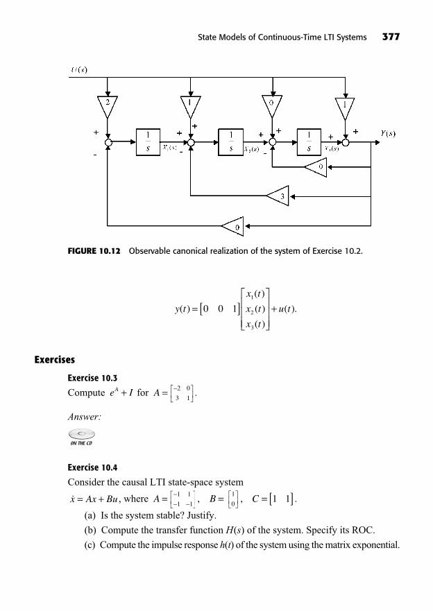
Exercises
Exercise 10.3
Compute for .
Answer:
Exercise 10.4
Consider the causal LTI state-space system
, where .
(a) Is the system stable? Justify.
(b) Compute the transfer function H(s) of the system. Specify its ROC.
(c) Compute the impulse response h(t) of the system using the matrix exponential.
C = [ ]1 1,1
0B =,1 1
1 1A =�x Ax Bu= +
2 0
3 1A =e IA +
y t
x t
x t
x t
u t( )
( )
( )
( )
( ).= [ ] +0 0 11
2
3
State Models of Continuous-Time LTI Systems 377
FIGURE 10.12 Observable canonical realization of the system of Exercise 10.2.
378 Fundamentals of Signals and Systems
Exercise 10.5
Repeat Exercise 10.4 with . What type of sys-tem is this?
(a) Is the system stable? Justify.
(b) Compute the transfer function H(s) of the system. Specify its ROC.
(c) Compute the impulse response h(t) of the system using the matrix expo-nential.
Answer:
Exercise 10.6
Find the controllable and observable canonical state-space realizations for each ofthe following LTI systems.
(a)
(b)
Exercise 10.7
Find the controllable and observable canonical state-space realizations for each ofthe following LTI systems.
(a)
(b)
(c) , , causal
Answer:
Exercise 10.8
(a) Compute for .A =0 1
3 2eA
yx
xu= [ ] +2 1 1
2
��x
x
x
x1
2
1
2
1 0
0 2
3
1= + u
s
s s ss
2
3 2
5
2 2 10 5
++ + +
>, Re{ } .
h t e q t e q t tt t( ) ( ) ( ) ( )= + +3
s s s
s s ss
3 2
3 2
2 1
5 20
+ + ++ +
>, Re{ }
h t e q t te q tt t( ) ( ) ( )= +2 2
C = [ ]0 1,0 0
1 0B =,0 0
1 0A =
State Models of Continuous-Time LTI Systems 379
(b) Compute the zero-input state and output responses at time for thecausal LTI state-space system
, y = Cx where ,
with initial state .
Exercise 10.9
Consider the causal LTI state-space system
, y = Cx where .
(a) Is the system minimal? Is it stable? Justify.
(b) Compute the transfer function H(s) of the system. Specify its ROC.
(c) Compute the state transition matrix defined as . This ma-trix has the property of taking the zero-input state response from the initialstate to the state x(t) as follows: .
(d) Compute the impulse response h(t) of the system using the matrix exponential.
Answer:
Exercise 10.10
Consider the LTI causal state-space system
where . Show that any state transformation ,where is invertible, of the above state-space system keeps its transferfunction invariant. This means that there are infinitely many state-space represen-tations of any given proper rational transfer function.
Q N N×Rz Qx=x t y t u tN( ) , ( ) , ( )R R R
�x Ax Bu
y Cx Du
= += + ,
x t t t x t( ) ( , ) ( )= 0 0x t( )0
( , ) : ( )t t eA t t0
0=
A B C= = = [ ]11 1
3 9
2
31 1, ,�x Ax Bu= +
x( )01
1=
A B C= = = [ ]0 1
3 2
0
11 0, ,�x Ax Bu= +
t1 2=

This page intentionally left blank
381
Application of TransformTechniques to LTI FeedbackControl Systems
11
In This Chapter
Introduction to LTI Feedback Control SystemsClosed-Loop Stability and the Root LocusThe Nyquist Stability CriterionStability Robustness: Gain and Phase MarginsSummaryTo Probe FurtherExercises
((Lecture 36: Introduction to LTI Feedback Control Systems))
The use of feedback dates back more than two thousand years to the Greeksand the Arabs, who invented the water clock based on a water level floatregulator. Closer to us, and marking the beginning of the industrial revolu-
tion in 1769, was the invention by James Watt of the Watt governor, shown in Fig-ure 11.1. The Watt governor was used to regulate automatically the speed of steamengines by feedback. This device measures the angular velocity of the engine shaftwith the help of the centrifugal force acting on two spinning masses hinged at the
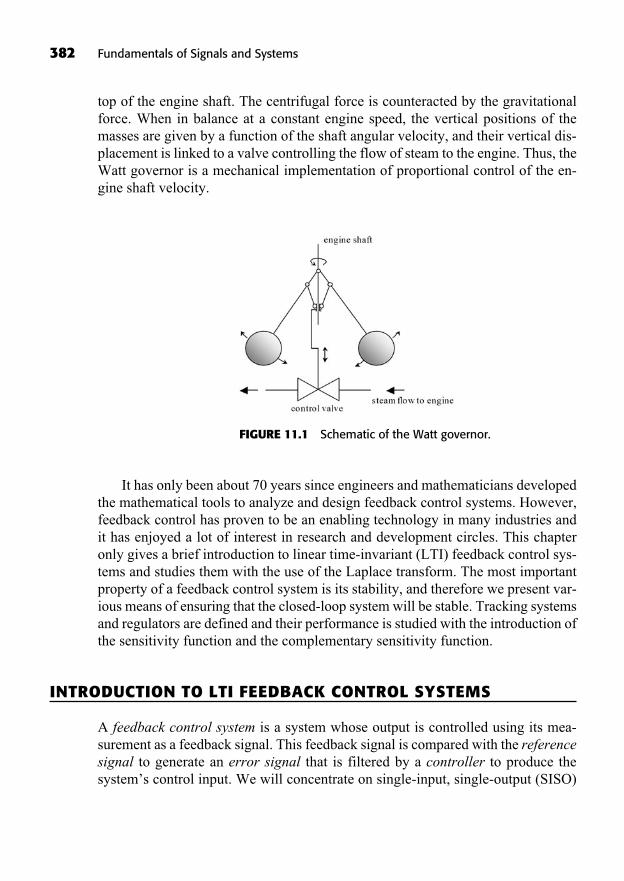
382 Fundamentals of Signals and Systems
top of the engine shaft. The centrifugal force is counteracted by the gravitationalforce. When in balance at a constant engine speed, the vertical positions of themasses are given by a function of the shaft angular velocity, and their vertical dis-placement is linked to a valve controlling the flow of steam to the engine. Thus, theWatt governor is a mechanical implementation of proportional control of the en-gine shaft velocity.
FIGURE 11.1 Schematic of the Watt governor.
It has only been about 70 years since engineers and mathematicians developedthe mathematical tools to analyze and design feedback control systems. However,feedback control has proven to be an enabling technology in many industries andit has enjoyed a lot of interest in research and development circles. This chapteronly gives a brief introduction to linear time-invariant (LTI) feedback control sys-tems and studies them with the use of the Laplace transform. The most importantproperty of a feedback control system is its stability, and therefore we present var-ious means of ensuring that the closed-loop system will be stable. Tracking systemsand regulators are defined and their performance is studied with the introduction ofthe sensitivity function and the complementary sensitivity function.
INTRODUCTION TO LTI FEEDBACK CONTROL SYSTEMS
A feedback control system is a system whose output is controlled using its mea-surement as a feedback signal. This feedback signal is compared with the referencesignal to generate an error signal that is filtered by a controller to produce thesystem’s control input. We will concentrate on single-input, single-output (SISO)
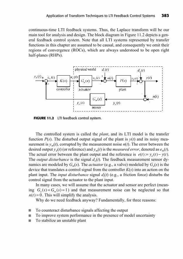
continuous-time LTI feedback systems. Thus, the Laplace transform will be ourmain tool for analysis and design. The block diagram in Figure 11.2 depicts a gen-eral feedback control system. Note that all LTI systems represented by transferfunctions in this chapter are assumed to be causal, and consequently we omit theirregions of convergence (ROCs), which are always understood to be open righthalf-planes (RHPs).
Application of Transform Techniques to LTI Feedback Control Systems 383
FIGURE 11.2 LTI feedback control system.
The controlled system is called the plant, and its LTI model is the transferfunction P(s). The disturbed output signal of the plant is y(t) and its noisy mea-surement is ym(t), corrupted by the measurement noise n(t). The error between thedesired output yd(t) (or reference) and ym(t) is the measured error, denoted as em(t).The actual error between the plant output and the reference is .The output disturbance is the signal do(t). The feedback measurement sensor dy-namics are modeled by Gm(s). The actuator (e.g., a valve) modeled by Ga(s) is thedevice that translates a control signal from the controller K(s) into an action on theplant input. The input disturbance signal di(t) (e.g., a friction force) disturbs thecontrol signal from the actuator to the plant input.
In many cases, we will assume that the actuator and sensor are perfect (mean-ing ) and that measurement noise can be neglected so that
. This will simplify the analysis.Why do we need feedback anyway? Fundamentally, for three reasons:
To counteract disturbance signals affecting the outputTo improve system performance in the presence of model uncertaintyTo stabilize an unstable plant
n t( ) = 0G s G sa m( ) ( )= = 1
e t y t y td( ) : ( ) ( )=
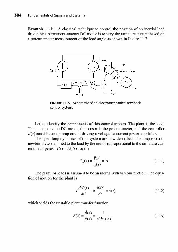
384 Fundamentals of Signals and Systems
Example 11.1: A classical technique to control the position of an inertial loaddriven by a permanent-magnet DC motor is to vary the armature current based ona potentiometer measurement of the load angle as shown in Figure 11.3.
FIGURE 11.3 Schematic of an electromechanical feedbackcontrol system.
Let us identify the components of this control system. The plant is the load.The actuator is the DC motor, the sensor is the potentiometer, and the controllerK(s) could be an op-amp circuit driving a voltage-to-current power amplifier.
The open-loop dynamics of this system are now described. The torque (t) innewton-meters applied to the load by the motor is proportional to the armature cur-rent in amperes: , so that
(11.1)
The plant (or load) is assumed to be an inertia with viscous friction. The equa-tion of motion for the plant is
(11.2)
which yields the unstable plant transfer function:
(11.3)P ss
s s Js b( )
ˆ( )ˆ( ) ( )
.= =+
1
Jd t
dtbd t
dtt
2
2
( ) ( )( )+ =
G ss
i sAa
a
( )ˆ( )ˆ ( )
.= =
( ) ( )t Ai ta=
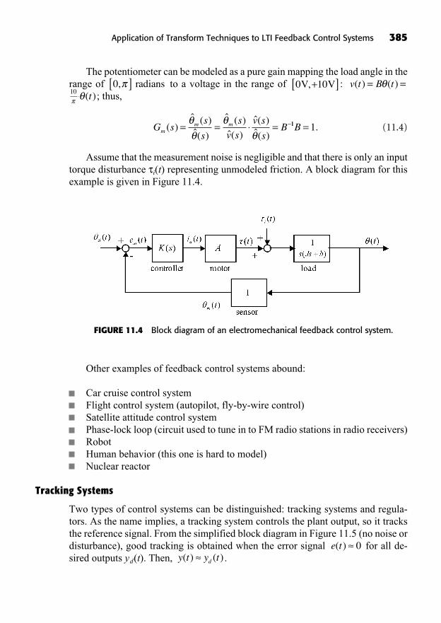
The potentiometer can be modeled as a pure gain mapping the load angle in therange of to a voltage in the range of :
; thus,
(11.4)
Assume that the measurement noise is negligible and that there is only an inputtorque disturbance i(t) representing unmodeled friction. A block diagram for thisexample is given in Figure 11.4.
G ss
s
s
v s
v s
sBm
m m( )ˆ ( )ˆ( )
ˆ ( )ˆ( )
ˆ( )ˆ( )
= = = 11 1B = .
t( )10v t B t( ) ( )= =0 10V V,+[ ]0,[ ] radians
Application of Transform Techniques to LTI Feedback Control Systems 385
FIGURE 11.4 Block diagram of an electromechanical feedback control system.
Other examples of feedback control systems abound:
Car cruise control systemFlight control system (autopilot, fly-by-wire control)Satellite attitude control systemPhase-lock loop (circuit used to tune in to FM radio stations in radio receivers)RobotHuman behavior (this one is hard to model)Nuclear reactor
Tracking Systems
Two types of control systems can be distinguished: tracking systems and regula-tors. As the name implies, a tracking system controls the plant output, so it tracksthe reference signal. From the simplified block diagram in Figure 11.5 (no noise ordisturbance), good tracking is obtained when the error signal for all de-sired outputs yd(t). Then, .y t y td( ) ( )
e t( ) 0
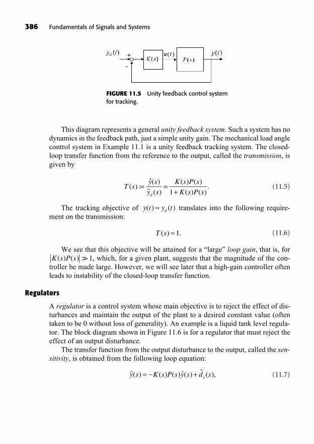
386 Fundamentals of Signals and Systems
This diagram represents a general unity feedback system. Such a system has nodynamics in the feedback path, just a simple unity gain. The mechanical load anglecontrol system in Example 11.1 is a unity feedback tracking system. The closed-loop transfer function from the reference to the output, called the transmission, isgiven by
(11.5)
The tracking objective of translates into the following require-ment on the transmission:
(11.6)
We see that this objective will be attained for a “large” loop gain, that is, for, which, for a given plant, suggests that the magnitude of the con-
troller be made large. However, we will see later that a high-gain controller oftenleads to instability of the closed-loop transfer function.
Regulators
A regulator is a control system whose main objective is to reject the effect of dis-turbances and maintain the output of the plant to a desired constant value (oftentaken to be 0 without loss of generality). An example is a liquid tank level regula-tor. The block diagram shown in Figure 11.6 is for a regulator that must reject theeffect of an output disturbance.
The transfer function from the output disturbance to the output, called the sen-sitivity, is obtained from the following loop equation:
(11.7)ˆ( ) ( ) ( ) ˆ( ) ˆ ( ),y s K s P s y s d so= +
K s P s( ) ( ) �1
T s( ) .1
y t y td( ) ( )
T sy s
y s
K s P s
K s P sd
( ) :ˆ( )ˆ ( )
( ) ( )
( ) ( ).= =
+1
FIGURE 11.5 Unity feedback control systemfor tracking.
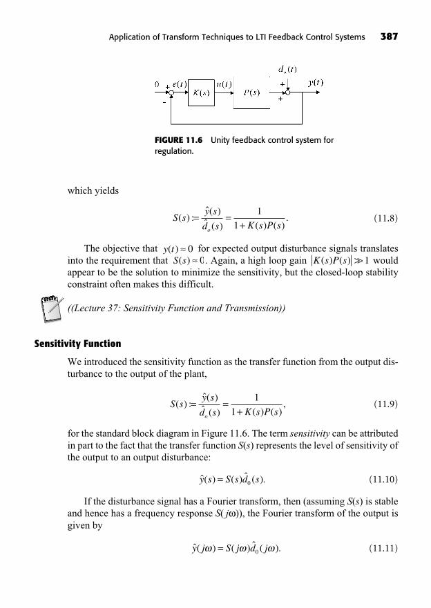
Application of Transform Techniques to LTI Feedback Control Systems 387
which yields
(11.8)
The objective that for expected output disturbance signals translatesinto the requirement that . Again, a high loop gain wouldappear to be the solution to minimize the sensitivity, but the closed-loop stabilityconstraint often makes this difficult.
((Lecture 37: Sensitivity Function and Transmission))
Sensitivity Function
We introduced the sensitivity function as the transfer function from the output dis-turbance to the output of the plant,
(11.9)
for the standard block diagram in Figure 11.6. The term sensitivity can be attributedin part to the fact that the transfer function S(s) represents the level of sensitivity ofthe output to an output disturbance:
(11.10)
If the disturbance signal has a Fourier transform, then (assuming S(s) is stableand hence has a frequency response S( j )), the Fourier transform of the output isgiven by
(11.11)ˆ( ) ( ) ˆ ( ).y j S j d j= 0
ˆ( ) ( ) ˆ ( ).y s S s d s= 0
S sy s
d s K s P so
( ) :ˆ( )ˆ ( ) ( ) ( )
,= =+
1
1
K s P s( ) ( ) �1S s( ) 0y t( ) 0
S sy s
d s K s P so
( ) :ˆ( )ˆ ( ) ( ) ( )
.= =+
1
1
FIGURE 11.6 Unity feedback control system forregulation.
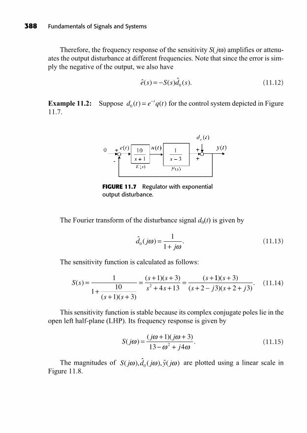
388 Fundamentals of Signals and Systems
Therefore, the frequency response of the sensitivity S( j ) amplifies or attenu-ates the output disturbance at different frequencies. Note that since the error is sim-ply the negative of the output, we also have
(11.12)
Example 11.2: Suppose for the control system depicted in Figure11.7.
d t e q tt0 ( ) ( )=
ˆ( ) ( ) ˆ ( ).e s S s d s= 0
FIGURE 11.7 Regulator with exponentialoutput disturbance.
The Fourier transform of the disturbance signal d0(t) is given by
(11.13)
The sensitivity function is calculated as follows:
(11.14)
This sensitivity function is stable because its complex conjugate poles lie in theopen left half-plane (LHP). Its frequency response is given by
(11.15)
The magnitudes of are plotted using a linear scale inFigure 11.8.
S j d j y j( ), ˆ ( ), ˆ( )0
S jj j
j( )
( )( ).=
+ ++
1 3
13 42
S s
s s
s s
s s
s( )
( )( )
( )( ) (=
++ +
=+ ++ +
=+1
110
1 3
1 3
4 132
11 3
2 3 2 3
)( )
( )( ).
s
s j s j
++ + +
ˆ ( ) .d jj0
1
1=
+
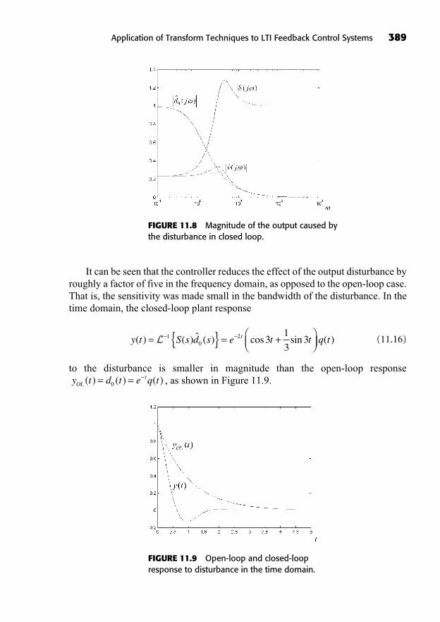
It can be seen that the controller reduces the effect of the output disturbance byroughly a factor of five in the frequency domain, as opposed to the open-loop case.That is, the sensitivity was made small in the bandwidth of the disturbance. In thetime domain, the closed-loop plant response
(11.16)
to the disturbance is smaller in magnitude than the open-loop response, as shown in Figure 11.9.y t d t e q tOL
t( ) ( ) ( )= =0
y t S s d s e t tt( ) ( ) ˆ ( ) cos sin= { } = +L 10
2 31
33 q t( )
Application of Transform Techniques to LTI Feedback Control Systems 389
FIGURE 11.8 Magnitude of the output caused bythe disturbance in closed loop.
FIGURE 11.9 Open-loop and closed-loopresponse to disturbance in the time domain.
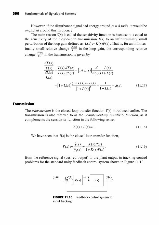
However, if the disturbance signal had energy around , it would beamplified around this frequency.
The main reason S(s) is called the sensitivity function is because it is equal tothe sensitivity of the closed-loop transmission T(s) to an infinitesimally smallperturbation of the loop gain defined as . That is, for an infinites-imally small relative change in the loop gain, the corresponding relative
change in the transmission is given by
(11.17)
Transmission
The transmission is the closed-loop transfer function T(s) introduced earlier. Thetransmission is also referred to as the complementary sensitivity function, as itcomplements the sensitivity function in the following sense:
(11.18)
We have seen that T(s) is the closed-loop transfer function,
(11.19)
from the reference signal (desired output) to the plant output in tracking controlproblems for the standard unity feedback control system shown in Figure 11.10.
T sy s
y s
K s P s
K s P sd
( ) :ˆ( )ˆ ( )
( ) ( )
( ) ( ),= =
+1
S s T s( ) ( ) .+ = 1
dT sT sdL sL s
L s
T s
dT s
dL sL s
( )( )( )( )
( )
( )
( )
( )(= = +1 ))
( )
( )
( )
( )( ( )) ( )
[ ]+
= +[ ] +
d
dL s
L s
L s
L sL s L s
1
11
1++[ ]=
+=
L s L sS s
( ) ( )( ).2
1
1
dT s
T s
( )
( )
dL s
L s
( )
( )
L s K s P s( ) : ( ) ( )=
= 4 rad/s
390 Fundamentals of Signals and Systems
FIGURE 11.10 Feedback control system forinput tracking.
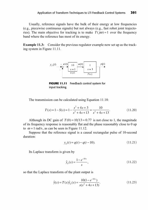
Usually, reference signals have the bulk of their energy at low frequencies(e.g., piecewise continuous signals) but not always (e.g., fast robot joint trajecto-ries). The main objective for tracking is to make over the frequencyband where the reference has most of its energy.
Example 11.3: Consider the previous regulator example now set up as the track-ing system in Figure 11.11.
T j( ) 1
Application of Transform Techniques to LTI Feedback Control Systems 391
FIGURE 11.11 Feedback control system forinput tracking.
The transmission can be calculated using Equation 11.18:
(11.20)
Although its DC gain of is not close to 1, the magnitudeof its frequency response is reasonably flat and the phase reasonably close to 0 upto , as can be seen in Figure 11.12.
Suppose that the reference signal is a causal rectangular pulse of 10-secondduration:
(11.21)
Its Laplace transform is given by
(11.22)
so that the Laplace transform of the plant output is
(11.23)ˆ( ) ( ) ˆ ( )( )
( ).y s T s y s
e
s s sd
s
= =+ +
10 1
4 13
10
2
ˆ ( ) ,y se
sd
s
=1 10
y t q t q td ( ) ( ) ( ).= 10
= 1 rad/s
T ( ) .0 10 13 0 77= =
T s S ss s
s s s s( ) ( ) .= =
+ ++ +
=+ +
1 14 3
4 13
10
4 13
2
2 2
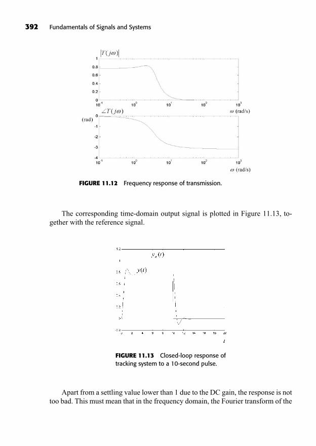
The corresponding time-domain output signal is plotted in Figure 11.13, to-gether with the reference signal.
392 Fundamentals of Signals and Systems
FIGURE 11.12 Frequency response of transmission.
FIGURE 11.13 Closed-loop response oftracking system to a 10-second pulse.
Apart from a settling value lower than 1 due to the DC gain, the response is nottoo bad. This must mean that in the frequency domain, the Fourier transform of the
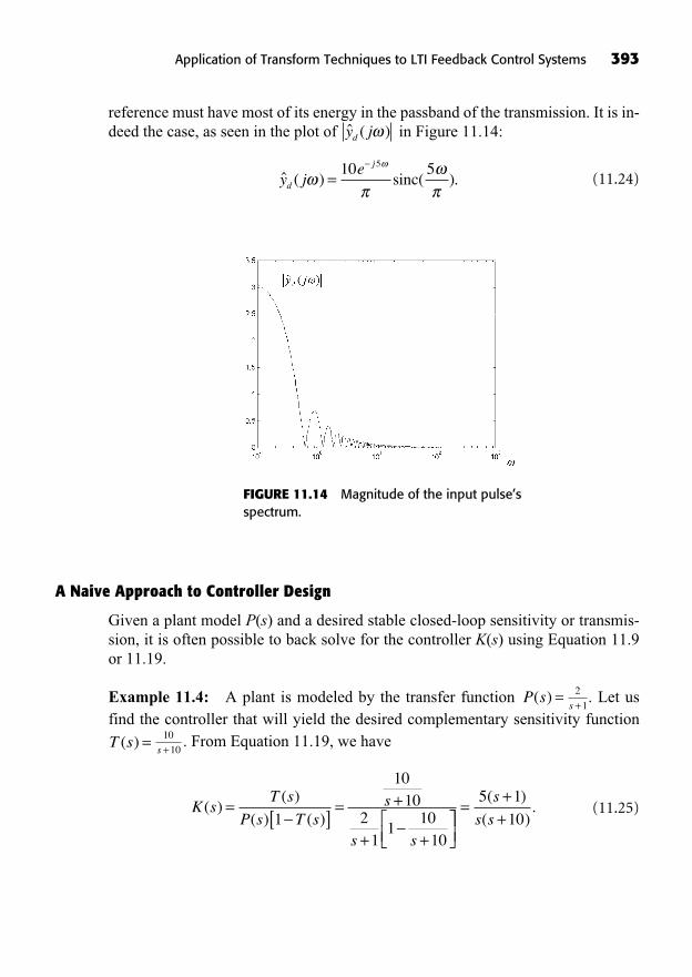
reference must have most of its energy in the passband of the transmission. It is in-deed the case, as seen in the plot of in Figure 11.14:
(11.24)ˆ ( ) ).y je
d
j
=10 5
sinc(5
ˆ ( )y jd
Application of Transform Techniques to LTI Feedback Control Systems 393
FIGURE 11.14 Magnitude of the input pulse’sspectrum.
A Naive Approach to Controller Design
Given a plant model P(s) and a desired stable closed-loop sensitivity or transmis-sion, it is often possible to back solve for the controller K(s) using Equation 11.9or 11.19.
Example 11.4: A plant is modeled by the transfer function . Let usfind the controller that will yield the desired complementary sensitivity function
. From Equation 11.19, we have
(11.25)K sT s
P s T ss
s s
( )( )
( ) ( )= [ ] =
+
+ +1
1010
21
110
10
=++
5 1
10
( )
( ).
s
s s
s +10
10T s( ) =
s +2
1P s( ) =
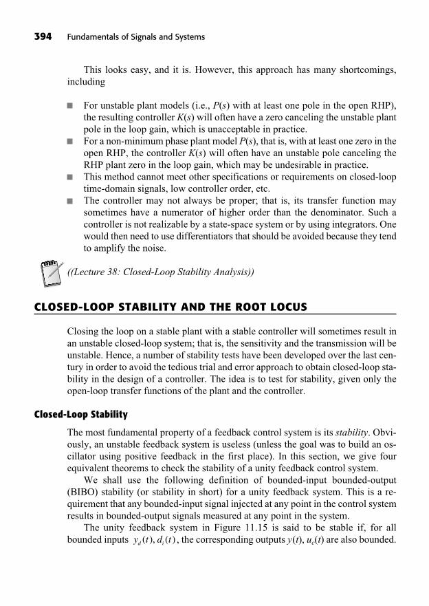
This looks easy, and it is. However, this approach has many shortcomings,including
For unstable plant models (i.e., P(s) with at least one pole in the open RHP),the resulting controller K(s) will often have a zero canceling the unstable plantpole in the loop gain, which is unacceptable in practice.For a non-minimum phase plant model P(s), that is, with at least one zero in theopen RHP, the controller K(s) will often have an unstable pole canceling theRHP plant zero in the loop gain, which may be undesirable in practice.This method cannot meet other specifications or requirements on closed-looptime-domain signals, low controller order, etc.The controller may not always be proper; that is, its transfer function maysometimes have a numerator of higher order than the denominator. Such acontroller is not realizable by a state-space system or by using integrators. Onewould then need to use differentiators that should be avoided because they tendto amplify the noise.
((Lecture 38: Closed-Loop Stability Analysis))
CLOSED-LOOP STABILITY AND THE ROOT LOCUS
Closing the loop on a stable plant with a stable controller will sometimes result inan unstable closed-loop system; that is, the sensitivity and the transmission will beunstable. Hence, a number of stability tests have been developed over the last cen-tury in order to avoid the tedious trial and error approach to obtain closed-loop sta-bility in the design of a controller. The idea is to test for stability, given only theopen-loop transfer functions of the plant and the controller.
Closed-Loop Stability
The most fundamental property of a feedback control system is its stability. Obvi-ously, an unstable feedback system is useless (unless the goal was to build an os-cillator using positive feedback in the first place). In this section, we give fourequivalent theorems to check the stability of a unity feedback control system.
We shall use the following definition of bounded-input bounded-output(BIBO) stability (or stability in short) for a unity feedback system. This is a re-quirement that any bounded-input signal injected at any point in the control systemresults in bounded-output signals measured at any point in the system.
The unity feedback system in Figure 11.15 is said to be stable if, for allbounded inputs , the corresponding outputs y(t), uc(t) are also bounded.y t d td i( ), ( )
394 Fundamentals of Signals and Systems
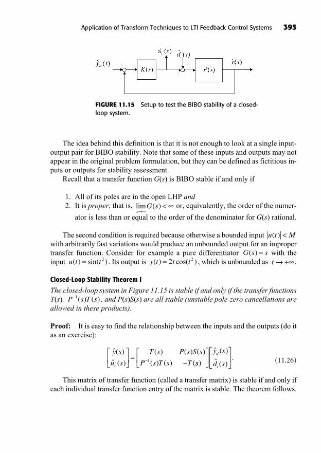
Application of Transform Techniques to LTI Feedback Control Systems 395
The idea behind this definition is that it is not enough to look at a single input-output pair for BIBO stability. Note that some of these inputs and outputs may notappear in the original problem formulation, but they can be defined as fictitious in-puts or outputs for stability assessment.
Recall that a transfer function G(s) is BIBO stable if and only if
1. All of its poles are in the open LHP and2. It is proper; that is, or, equivalently, the order of the numer-
ator is less than or equal to the order of the denominator for G(s) rational.
The second condition is required because otherwise a bounded input with arbitrarily fast variations would produce an unbounded output for an impropertransfer function. Consider for example a pure differentiator with theinput . Its output is , which is unbounded as .
Closed-Loop Stability Theorem I
The closed-loop system in Figure 11.15 is stable if and only if the transfer functionsT(s), , and P(s)S(s) are all stable (unstable pole-zero cancellations areallowed in these products).
Proof: It is easy to find the relationship between the inputs and the outputs (do itas an exercise):
(11.26)
This matrix of transfer function (called a transfer matrix) is stable if and only ifeach individual transfer function entry of the matrix is stable. The theorem follows.
ˆ( )
ˆ ( )
( ) ( ) ( )
( ) ( ) (
y s
u s
T s P s S s
P s T s Tc
= 1 ss
y s
d s
d
i)
ˆ ( )
ˆ ( ).
P s T s1( ) ( )
t +y t t t( ) cos( )= 2 2u t t( ) sin( )= 2G s s( ) =
u t M( ) <
lim ( )s
G s <
FIGURE 11.15 Setup to test the BIBO stability of a closed-loop system.
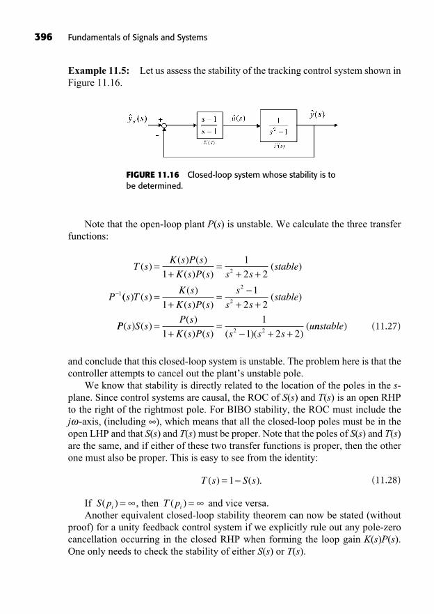
Example 11.5: Let us assess the stability of the tracking control system shown inFigure 11.16.
396 Fundamentals of Signals and Systems
FIGURE 11.16 Closed-loop system whose stability is tobe determined.
Note that the open-loop plant P(s) is unstable. We calculate the three transferfunctions:
(11.27)
and conclude that this closed-loop system is unstable. The problem here is that thecontroller attempts to cancel out the plant’s unstable pole.
We know that stability is directly related to the location of the poles in the s-plane. Since control systems are causal, the ROC of S(s) and T(s) is an open RHPto the right of the rightmost pole. For BIBO stability, the ROC must include the j -axis, (including ), which means that all the closed-loop poles must be in theopen LHP and that S(s) and T(s) must be proper. Note that the poles of S(s) and T(s)are the same, and if either of these two transfer functions is proper, then the otherone must also be proper. This is easy to see from the identity:
(11.28)
If , then and vice versa.Another equivalent closed-loop stability theorem can now be stated (without
proof) for a unity feedback control system if we explicitly rule out any pole-zerocancellation occurring in the closed RHP when forming the loop gain K(s)P(s).One only needs to check the stability of either S(s) or T(s).
T pi( ) =S pi( ) =
T s S s( ) ( ).= 1
T sK s P s
K s P s s sstable
P
( )( ) ( )
( ) ( )( )=
+=
+ +1
1
2 22
1(( ) ( )( )
( ) ( )( )s T s
K s
K s P s
s
s sstable=
+=
+ +1
1
2 2
2
2
PP s S sP s
K s P s s s su( ) ( )
( )
( ) ( ) ( )( )(=
+=
+ +1
1
1 2 22 2 nnstable)
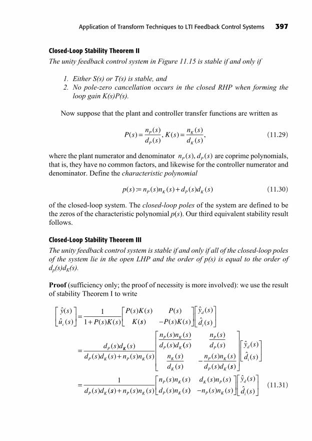
Closed-Loop Stability Theorem II
The unity feedback control system in Figure 11.15 is stable if and only if
1. Either S(s) or T(s) is stable, and2. No pole-zero cancellation occurs in the closed RHP when forming the
loop gain K(s)P(s).
Now suppose that the plant and controller transfer functions are written as
(11.29)
where the plant numerator and denominator are coprime polynomials,that is, they have no common factors, and likewise for the controller numerator anddenominator. Define the characteristic polynomial
(11.30)
of the closed-loop system. The closed-loop poles of the system are defined to bethe zeros of the characteristic polynomial p(s). Our third equivalent stability resultfollows.
Closed-Loop Stability Theorem III
The unity feedback control system is stable if and only if all of the closed-loop polesof the system lie in the open LHP and the order of p(s) is equal to the order ofdp(s)dK(s).
Proof (sufficiency only; the proof of necessity is more involved): we use the resultof stability Theorem I to write
(11.31)
ˆ( )
ˆ ( ) ( ) ( )
( ) ( ) ( )
(
y s
u s P s K s
P s K s P s
Kc
=+
1
1 ss P s K s
y s
d s
d s d
d
i
P
) ( ) ( )
ˆ ( )
ˆ ( )
( )= KK
P K P K
P K
P Ks
d s d s n s n s
n s n s
d s d( )
( ) ( ) ( ) ( )
( ) ( )
( )
+(( )
( )
( )
( )
( )
( ) ( )
( ) (
s
n s
d s
n s
d s
n s n s
d s d
P
P
K
K
P K
P K ss
y s
d s
d s d
d
i
P K
)
ˆ ( )
ˆ ( )
( ) (=
1
ss n s n s
n s n s d s n s
d s n sP K
P K K P
P K) ( ) ( )
( ) ( ) ( ) ( )
( ) (+ )) ( ) ( )
ˆ ( )
ˆ ( )n s n s
y s
d sP K
d
i
p s n s n s d s d sP K P K( ) : ( ) ( ) ( ) ( )= +
n s d sP P( ), ( )
P sn s
d sK s
n s
d sP
P
K
K
( )( )
( ), ( )
( )
( ),= =
Application of Transform Techniques to LTI Feedback Control Systems 397
All transfer functions in this matrix are proper and have the characteristic poly-nomial p(s) as their denominator. Therefore, if all closed-loop poles (i.e., zeros ofp(s)) are in the open LHP, then the transfer matrix is stable, and by virtue of The-orem I, we conclude that the closed-loop system is stable.
Example 11.6: For Example 11.5, we have
(11.32)
and
(11.33)
which clearly has a zero at s = 1. Therefore the control system is unstable.Finally, we have a fourth equivalent theorem on closed-loop stability, which is
really just a restatement of Theorem II (taking S(s)).
Closed-Loop Stability Theorem IV
The unity feedback control system is stable if and only if
1. The transfer function 1 + K(s)P(s) has no closed RHP zeros (including at ),and
2. No pole-zero cancellation occurs in the closed RHP when forming theloop gain K(s)P(s).
Routh’s Criterion
The stability of a causal LTI system whose transfer function is rational and proper isdetermined by its poles. An open-loop transfer function is stable if and only if all ofits poles lie in the open LHP. A closed-loop system is stable if and only if all of the closed-loop poles lie in the open LHP (closed-loop theorem III). In both cases,we need to solve for the N roots of the characteristic equation
to find the poles and determine whether thesystem is stable or not. There are various ways to do this numerically using a com-puter, for example, by computing the eigenvalues of the A matrix of a state-space re-alization of the system. However, in 1877, E. J. Routh devised an extremely simpleand clever technique to determine the stability of a system. Routh’s criterion is basedon an array formed with the coefficients of the denominator of an open-loop transferfunction or the closed-loop characteristic polynomial of a feedback system. Assumethat , and recall that a necessary condition for the system to be stable is thatall coefficients of its characteristic polynomial be of the same sign. Thus, if any of thecoefficients of the polynomial are negative, the system is unstable. With this neces-sary condition fulfilled, we want to determine whether the system is stable or not.
aN > 0
a s a s a s aNN
NN+ + + + =1
11 0 0
p s s s s( ) ( ) ( ) ( ),= + +1 1 12
n s d s s s n s s d sP P K K( ) , ( ) ( )( ), ( ) ( ), ( )= = + = =1 1 1 1 (( )s +1
398 Fundamentals of Signals and Systems
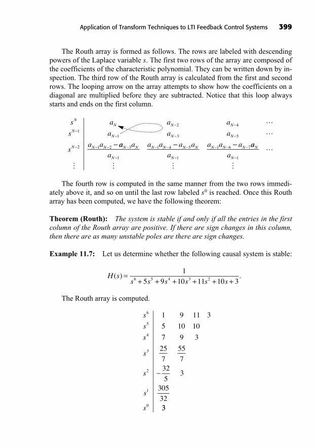
The Routh array is formed as follows. The rows are labeled with descendingpowers of the Laplace variable s. The first two rows of the array are composed ofthe coefficients of the characteristic polynomial. They can be written down by in-spection. The third row of the Routh array is calculated from the first and secondrows. The looping arrow on the array attempts to show how the coefficients on adiagonal are multiplied before they are subtracted. Notice that this loop alwaysstarts and ends on the first column.
The fourth row is computed in the same manner from the two rows immedi-ately above it, and so on until the last row labeled s0 is reached. Once this Routharray has been computed, we have the following theorem:
Theorem (Routh): The system is stable if and only if all the entries in the firstcolumn of the Routh array are positive. If there are sign changes in this column,then there are as many unstable poles are there are sign changes.
Example 11.7: Let us determine whether the following causal system is stable:
The Routh array is computed.
s
s
s
s
s
s
s
6
5
4
3
2
1
0
1 9 11 3
5 10 10
7 9 3
25
7
55
732
53
305
3233
H ss s s s s s
( ) .=+ + + + + +
1
5 9 10 11 10 36 5 4 3 2
s a a a
s a a a
sa a
NN N N
NN N N
N N N
2 41
1 3 5
2 1 2
aa a
a
a a a a
a
a a aN N
N
N N N N
N
N N N3
1
1 4 5
1
1 6 7aa
aN
N 1
� � � �
Application of Transform Techniques to LTI Feedback Control Systems 399
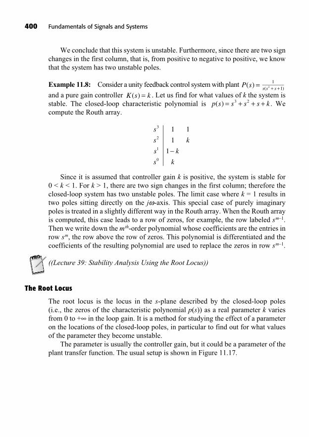
We conclude that this system is unstable. Furthermore, since there are two signchanges in the first column, that is, from positive to negative to positive, we knowthat the system has two unstable poles.
Example 11.8: Consider a unity feedback control system with plant
and a pure gain controller . Let us find for what values of k the system isstable. The closed-loop characteristic polynomial is . Wecompute the Routh array.
Since it is assumed that controller gain k is positive, the system is stable for 0 < k < 1. For k > 1, there are two sign changes in the first column; therefore theclosed-loop system has two unstable poles. The limit case where k = 1 results intwo poles sitting directly on the j -axis. This special case of purely imaginarypoles is treated in a slightly different way in the Routh array. When the Routh arrayis computed, this case leads to a row of zeros, for example, the row labeled sm–1.Then we write down the mth-order polynomial whose coefficients are the entries inrow sm, the row above the row of zeros. This polynomial is differentiated and thecoefficients of the resulting polynomial are used to replace the zeros in row sm–1.
((Lecture 39: Stability Analysis Using the Root Locus))
The Root Locus
The root locus is the locus in the s-plane described by the closed-loop poles (i.e., the zeros of the characteristic polynomial p(s)) as a real parameter k variesfrom 0 to + in the loop gain. It is a method for studying the effect of a parameteron the locations of the closed-loop poles, in particular to find out for what valuesof the parameter they become unstable.
The parameter is usually the controller gain, but it could be a parameter of theplant transfer function. The usual setup is shown in Figure 11.17.
s
s k
s k
s k
3
2
1
0
1 1
1
1
p s s s s k( ) = + + +3 2K s k( ) =
s s s( )+ +1
12P s( ) =
400 Fundamentals of Signals and Systems
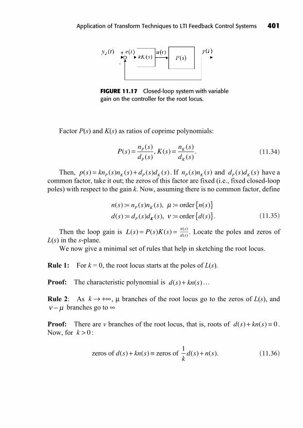
Application of Transform Techniques to LTI Feedback Control Systems 401
Factor P(s) and K(s) as ratios of coprime polynomials:
(11.34)
Then, . If and have acommon factor, take it out; the zeros of this factor are fixed (i.e., fixed closed-looppoles) with respect to the gain k. Now, assuming there is no common factor, define
(11.35)
Then the loop gain is . Locate the poles and zeros ofL(s) in the s-plane.
We now give a minimal set of rules that help in sketching the root locus.
Rule 1: For k = 0, the root locus starts at the poles of L(s).
Proof: The characteristic polynomial is …
Rule 2: As , μ branches of the root locus go to the zeros of L(s), andbranches go to
Proof: There are v branches of the root locus, that is, roots of .Now, for :
(11.36)zeros of zeros of 1
d s kn skd s n s( ) ( ) ( ) ( ).+ +
k > 0d s kn s( ) ( )+ = 0
μk +
d s kn s( ) ( )+
n s
d s
( )
( )L s P s K s( ) ( ) ( )= =
n s n s n s n s
d s d s dP K
P
( ) : ( ) ( ), : ( )
( ) : ( )
= = { }=
μ order
KK s d s( ), : ( ) .= { }order
d s d sP K( ) ( )n s n sP K( ) ( )p s kn s n s d s d sP K P K( ) ( ) ( ) ( ) ( )= +
P sn s
d sK s
n s
d sP
P
K
K
( )( )
( ), ( )
( )
( ).= =
FIGURE 11.17 Closed-loop system with variablegain on the controller for the root locus.
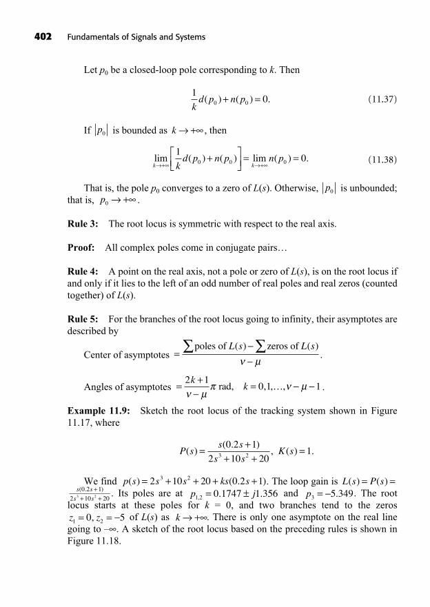
Let p0 be a closed-loop pole corresponding to k. Then
(11.37)
If is bounded as , then
(11.38)
That is, the pole p0 converges to a zero of L(s). Otherwise, is unbounded;that is, .
Rule 3: The root locus is symmetric with respect to the real axis.
Proof: All complex poles come in conjugate pairs…
Rule 4: A point on the real axis, not a pole or zero of L(s), is on the root locus ifand only if it lies to the left of an odd number of real poles and real zeros (countedtogether) of L(s).
Rule 5: For the branches of the root locus going to infinity, their asymptotes aredescribed by
Center of asymptotes .
Angles of asymptotes .
Example 11.9: Sketch the root locus of the tracking system shown in Figure11.17, where
We find . The loop gain is . Its poles are at and . The root
locus starts at these poles for k = 0, and two branches tend to the zerosof L(s) as . There is only one asymptote on the real line
going to – . A sketch of the root locus based on the preceding rules is shown inFigure 11.18.
k +z z1 20 5= =,
p3 5 349= .p j1 2 0 1747 1 356, . .= ±s s
s s
( . )++ +0 2 1
2 10 203 2
L s P s( ) ( )= =p s s s ks s( ) ( . )= + + + +2 10 20 0 2 13 2
P ss s
s sK s( )
( . ), ( ) .=
++ +
=0 2 1
2 10 2013 2
=+
=2 1
0 1 1k
kμ
μrad, , , ,…
=poles of zeros of L s L s( ) ( )
μ
p0 +p0
lim ( ) ( ) lim ( ) .k kk
d p n p n p+ +
+ = =1
0 0 0 0
k +p0
100 0k
d p n p( ) ( ) .+ =
402 Fundamentals of Signals and Systems
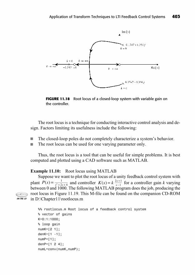
Application of Transform Techniques to LTI Feedback Control Systems 403
The root locus is a technique for conducting interactive control analysis and de-sign. Factors limiting its usefulness include the following:
The closed-loop poles do not completely characterize a system’s behavior.The root locus can be used for one varying parameter only.
Thus, the root locus is a tool that can be useful for simple problems. It is bestcomputed and plotted using a CAD software such as MATLAB.
Example 11.10: Root locus using MATLABSuppose we want to plot the root locus of a unity feedback control system with
plant and controller for a controller gain k varyingbetween 0 and 1000. The following MATLAB program does the job, producing theroot locus in Figure 11.19. This M-file can be found on the companion CD-ROMin D:\Chapter11\rootlocus.m
%% rootlocus.m Root locus of a feedback control system
% vector of gains
K=0:1:1000;
% loop gain
numK=[2 1];
denK=[1 -1];
numP=[1];
denP=[1 2 4];
numL=conv(numK,numP);
s
s
+2 1
1K s k( ) =s s+ +
1
2 42P s( ) =
FIGURE 11.18 Root locus of a closed-loop system with variable gain onthe controller.
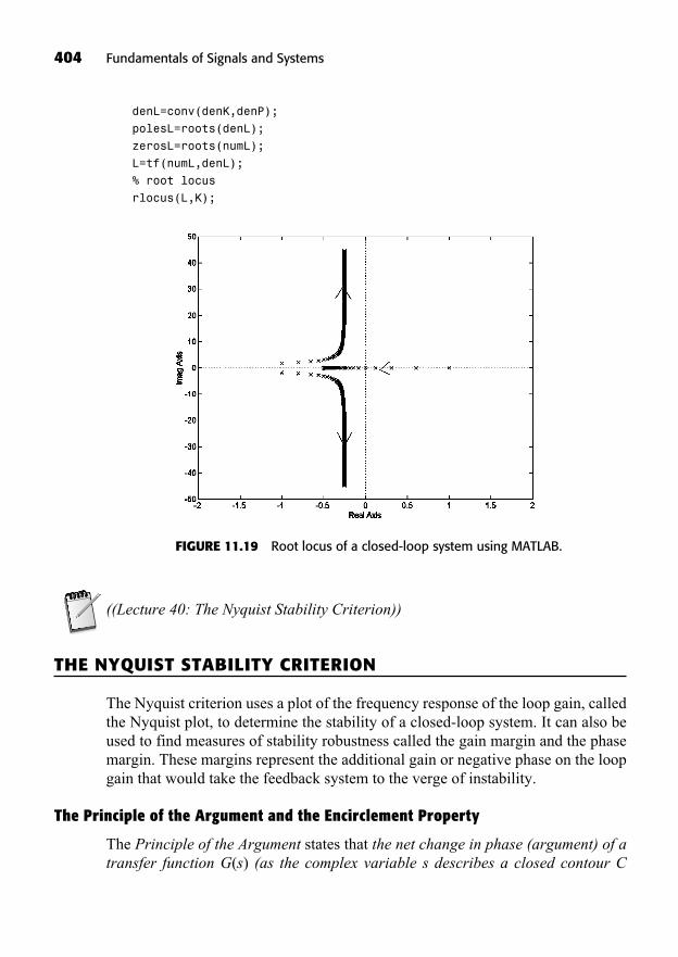
404 Fundamentals of Signals and Systems
denL=conv(denK,denP);
polesL=roots(denL);
zerosL=roots(numL);
L=tf(numL,denL);
% root locus
rlocus(L,K);
FIGURE 11.19 Root locus of a closed-loop system using MATLAB.
((Lecture 40: The Nyquist Stability Criterion))
THE NYQUIST STABILITY CRITERION
The Nyquist criterion uses a plot of the frequency response of the loop gain, calledthe Nyquist plot, to determine the stability of a closed-loop system. It can also beused to find measures of stability robustness called the gain margin and the phasemargin. These margins represent the additional gain or negative phase on the loopgain that would take the feedback system to the verge of instability.
The Principle of the Argument and the Encirclement Property
The Principle of the Argument states that the net change in phase (argument) of atransfer function G(s) (as the complex variable s describes a closed contour C
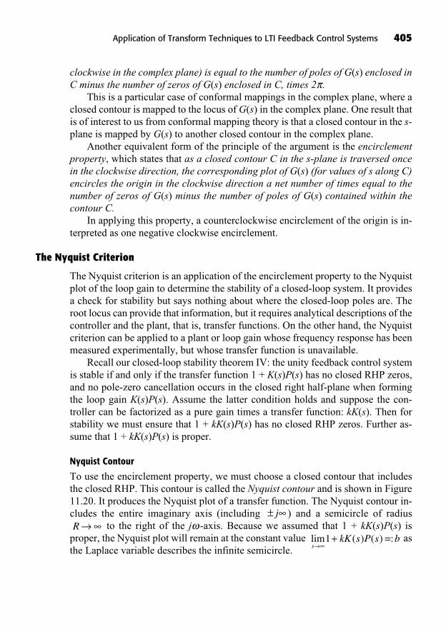
clockwise in the complex plane) is equal to the number of poles of G(s) enclosed inC minus the number of zeros of G(s) enclosed in C, times 2 .
This is a particular case of conformal mappings in the complex plane, where aclosed contour is mapped to the locus of G(s) in the complex plane. One result thatis of interest to us from conformal mapping theory is that a closed contour in the s-plane is mapped by G(s) to another closed contour in the complex plane.
Another equivalent form of the principle of the argument is the encirclementproperty, which states that as a closed contour C in the s-plane is traversed oncein the clockwise direction, the corresponding plot of G(s) (for values of s along C)encircles the origin in the clockwise direction a net number of times equal to thenumber of zeros of G(s) minus the number of poles of G(s) contained within thecontour C.
In applying this property, a counterclockwise encirclement of the origin is in-terpreted as one negative clockwise encirclement.
The Nyquist Criterion
The Nyquist criterion is an application of the encirclement property to the Nyquistplot of the loop gain to determine the stability of a closed-loop system. It providesa check for stability but says nothing about where the closed-loop poles are. Theroot locus can provide that information, but it requires analytical descriptions of thecontroller and the plant, that is, transfer functions. On the other hand, the Nyquistcriterion can be applied to a plant or loop gain whose frequency response has beenmeasured experimentally, but whose transfer function is unavailable.
Recall our closed-loop stability theorem IV: the unity feedback control systemis stable if and only if the transfer function 1 + K(s)P(s) has no closed RHP zeros,and no pole-zero cancellation occurs in the closed right half-plane when formingthe loop gain K(s)P(s). Assume the latter condition holds and suppose the con-troller can be factorized as a pure gain times a transfer function: kK(s). Then forstability we must ensure that 1 + kK(s)P(s) has no closed RHP zeros. Further as-sume that 1 + kK(s)P(s) is proper.
Nyquist Contour
To use the encirclement property, we must choose a closed contour that includesthe closed RHP. This contour is called the Nyquist contour and is shown in Figure11.20. It produces the Nyquist plot of a transfer function. The Nyquist contour in-cludes the entire imaginary axis (including ) and a semicircle of radius
to the right of the j -axis. Because we assumed that 1 + kK(s)P(s) isproper, the Nyquist plot will remain at the constant value asthe Laplace variable describes the infinite semicircle.
lim ( ) ( ) :s
kK s P s b+ =1R
± j
Application of Transform Techniques to LTI Feedback Control Systems 405
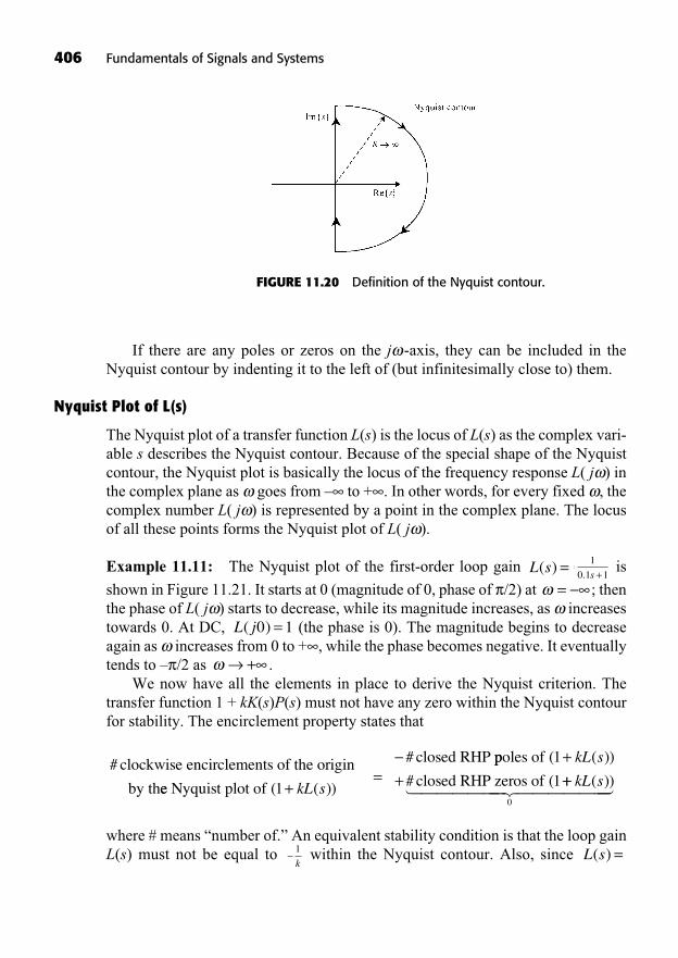
406 Fundamentals of Signals and Systems
If there are any poles or zeros on the j -axis, they can be included in theNyquist contour by indenting it to the left of (but infinitesimally close to) them.
Nyquist Plot of L(s)
The Nyquist plot of a transfer function L(s) is the locus of L(s) as the complex vari-able s describes the Nyquist contour. Because of the special shape of the Nyquistcontour, the Nyquist plot is basically the locus of the frequency response L( j ) inthe complex plane as goes from – to + . In other words, for every fixed , thecomplex number L( j ) is represented by a point in the complex plane. The locusof all these points forms the Nyquist plot of L( j ).
Example 11.11: The Nyquist plot of the first-order loop gain is
shown in Figure 11.21. It starts at 0 (magnitude of 0, phase of /2) at ; thenthe phase of L( j ) starts to decrease, while its magnitude increases, as increasestowards 0. At DC, (the phase is 0). The magnitude begins to decreaseagain as increases from 0 to + , while the phase becomes negative. It eventuallytends to – /2 as .
We now have all the elements in place to derive the Nyquist criterion. Thetransfer function 1 + kK(s)P(s) must not have any zero within the Nyquist contourfor stability. The encirclement property states that
where # means “number of.” An equivalent stability condition is that the loop gainL(s) must not be equal to within the Nyquist contour. Also, since L s( ) =1
k
# clockwise encirclements of the origin
by thee Nyquist plot of
closed RHP
( ( ))
#
1+=
kL s
ppoles of
closed RHP zeros of
( ( ))
# (
1
1
++
kL s
++ kL s( ))0
� ������� �������
+
L j( )0 1=
=s.
=+
1
0 1 1L s( ) =
FIGURE 11.20 Definition of the Nyquist contour.
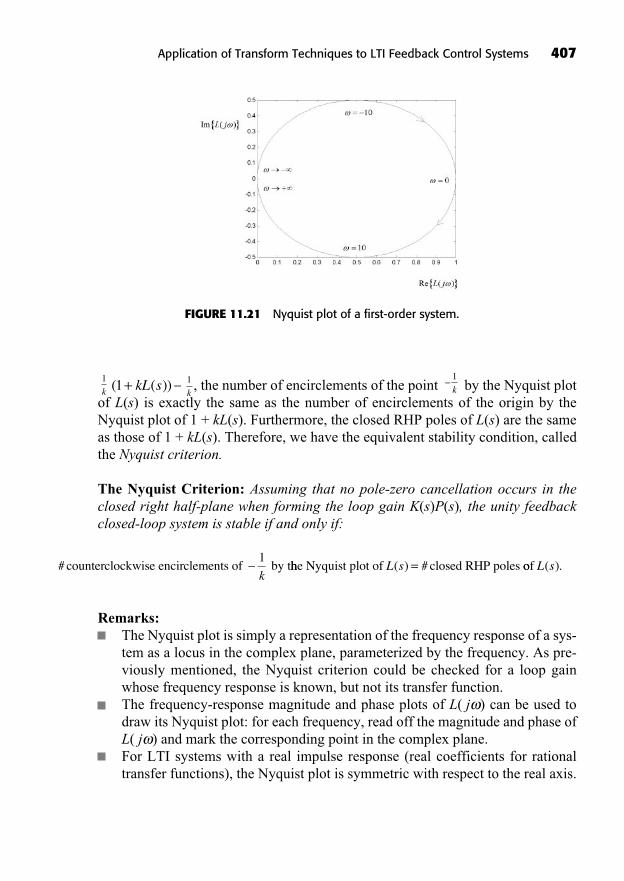
, the number of encirclements of the point by the Nyquist plotof L(s) is exactly the same as the number of encirclements of the origin by theNyquist plot of 1 + kL(s). Furthermore, the closed RHP poles of L(s) are the sameas those of 1 + kL(s). Therefore, we have the equivalent stability condition, calledthe Nyquist criterion.
The Nyquist Criterion: Assuming that no pole-zero cancellation occurs in theclosed right half-plane when forming the loop gain K(s)P(s), the unity feedbackclosed-loop system is stable if and only if:
Remarks:The Nyquist plot is simply a representation of the frequency response of a sys-tem as a locus in the complex plane, parameterized by the frequency. As pre-viously mentioned, the Nyquist criterion could be checked for a loop gainwhose frequency response is known, but not its transfer function.The frequency-response magnitude and phase plots of L( j ) can be used todraw its Nyquist plot: for each frequency, read off the magnitude and phase ofL( j ) and mark the corresponding point in the complex plane.For LTI systems with a real impulse response (real coefficients for rationaltransfer functions), the Nyquist plot is symmetric with respect to the real axis.
# counterclockwise encirclements of by t1
khhe Nyquist plot of closed RHP poles L s( ) #= oof L s( ).
1
kk
1kL s( ( ))+1k
1
Application of Transform Techniques to LTI Feedback Control Systems 407
FIGURE 11.21 Nyquist plot of a first-order system.
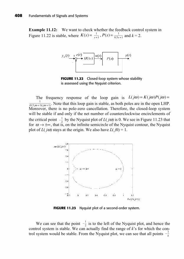
408 Fundamentals of Signals and Systems
Example 11.12: We want to check whether the feedback control system in Figure 11.22 is stable, where and k = 2.s.
=+
1
0 5 1P s, ( ) =
s +1
1K s( ) =
FIGURE 11.22 Closed-loop system whose stabilityis assessed using the Nyquist criterion.
The frequency response of the loop gain is . Note that this loop gain is stable, as both poles are in the open LHP.
Moreover, there is no pole-zero cancellation. Therefore, the closed-loop systemwill be stable if and only if the net number of counterclockwise encirclements ofthe critical point by the Nyquist plot of L( j ) is 0. We see in Figure 11.23 thatfor , that is, on the infinite semicircle of the Nyquist contour, the Nyquistplot of L( j ) stays at the origin. We also have L( j0) = 1.
±
1
2
j j( . )( )+ +1
0 5 1 1
L j K j P j( ) ( ) ( )= =
FIGURE 11.23 Nyquist plot of a second-order system.
We can see that the point is to the left of the Nyquist plot, and hence thecontrol system is stable. We can actually find the range of k’s for which the con-trol system would be stable. From the Nyquist plot, we can see that all points
1
k
1
2

to the left of the origin lie outside of the loop formed by the Nyquist plot, as wellas all points to the right of 1. This implies that the system is stable for andfor . Therefore the complete range of gains to get stability is .
((Lecture 41: Gain and Phase Margins))
STABILITY ROBUSTNESS: GAIN AND PHASE MARGINS
Bode Plot of Loop Gain
The Nyquist criterion gives us the ability to check the stability of a unity feedbacksystem by looking at the Nyquist plot of its loop gain only. This is useful for at leasttwo reasons.
We can design a controller K(s) based on a plant transfer function P(s) or just its frequency response P( j ) and ensure that the closed-loop system will be stable by looking at the frequency response of the loop gain
. We do not have to compute the characteristic polyno-mial (which cannot be done anyway if only P( j ) is available).Closed-loop stability robustness can be assessed by looking at the Nyquistplot. Stability robustness refers to how much variation in the loop gain’s fre-quency response L( j ) (mostly coming from uncertainty in the plant’s fre-quency response) can be tolerated without inducing instability of the controlsystem. Think of stability robustness as how far away the Nyquist plot is fromthe critical point . Here we are assuming that the Nyquist criterion was sat-isfied to start with, meaning that the nominal closed-loop system is stable. Inthis case, the closed loop will become unstable when L( j ) varies to the pointof touching the critical point .
Note that we will set k = 1 in the remainder of this section, such that the criti-cal point is now –1, that is, the controller is thought to be the fixed transfer func-tion K(s). An example is shown in Figure 11.24, where the nominal Nyquist plot ofL( j ) (no closed RHP poles in L(s)) of a closed-loop stable system is perturbed toLp( j ), which touches the critical point 1. The closed-loop system with loop gainLp( j ) is unstable.
By conjugate symmetry, the magnitude and phase plots (the Bode plot) of theloop gain’s frequency response L( j ) convey the same information as the Nyquistplot. Therefore, it is possible to use the Nyquist criterion to check closed-loop sta-bility by looking at the Bode plot of L( j ), although this often proves to be diffi-cult. It is relatively easy only for low-order, “well-behaved” loop gains, which
1
k
1
k
L j K j P j( ) ( ) ( )=
k > 1< <1 0kk 0
Application of Transform Techniques to LTI Feedback Control Systems 409
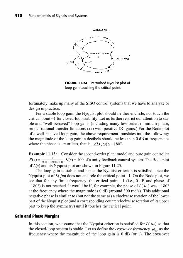
410 Fundamentals of Signals and Systems
FIGURE 11.24 Perturbed Nyquist plot ofloop gain touching the critical point.
fortunately make up many of the SISO control systems that we have to analyze ordesign in practice.
For a stable loop gain, the Nyquist plot should neither encircle, nor touch thecritical point 1 for closed-loop stability. Let us further restrict our attention to sta-ble and “well-behaved” loop gains (including many low-order, minimum-phase,proper rational transfer functions L(s) with positive DC gains.) For the Bode plotof a well-behaved loop gain, the above requirement translates into the following:the magnitude of the loop gain in decibels should be less than 0 dB at frequencieswhere the phase is – or less, that is, °.
Example 11.13: Consider the second-order plant model and pure gain controller , K(s) = 100 of a unity feedback control system. The Bode plot
of L(s) and its Nyquist plot are shown in Figure 11.25.The loop gain is stable, and hence the Nyquist criterion is satisfied since the
Nyquist plot of L( j ) does not encircle the critical point 1. On the Bode plot, wesee that for any finite frequency, the critical point 1 (i.e., 0 dB and phase of
180°) is not reached. It would be if, for example, the phase of L( j ) was 180°at the frequency where the magnitude is 0 dB (around 300 rad/s). This additionalnegative phase is similar to (but not the same as) a clockwise rotation of the lowerpart of the Nyquist plot (and a corresponding counterclockwise rotation of its upperpart to keep the symmetry) until it touches the critical point.
Gain and Phase Margins
In this section, we assume that the Nyquist criterion is satisfied for L( j ) so thatthe closed-loop system is stable. Let us define the crossover frequency as thefrequency where the magnitude of the loop gain is 0 dB (or 1). The crossover
co
s s( . )( . )+ +1
0 1 1 0 01 1P s( ) =
L j( ) 180
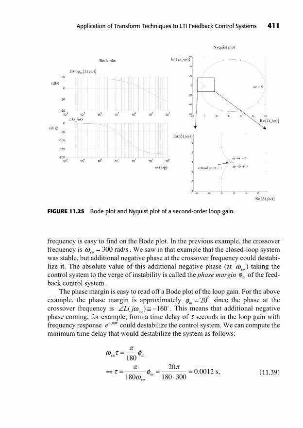
frequency is easy to find on the Bode plot. In the previous example, the crossoverfrequency is . We saw in that example that the closed-loop systemwas stable, but additional negative phase at the crossover frequency could destabi-lize it. The absolute value of this additional negative phase (at ) taking thecontrol system to the verge of instability is called the phase margin of the feed-back control system.
The phase margin is easy to read off a Bode plot of the loop gain. For the aboveexample, the phase margin is approximately since the phase at thecrossover frequency is . This means that additional negativephase coming, for example, from a time delay of seconds in the loop gain withfrequency response could destabilize the control system. We can compute theminimum time delay that would destabilize the system as follows:
(11.39)
co m
com
=
= = =
180
180
20
180 3000 0012. s,
e j
L j co( ) 160�m = 200
m
co
co = 300 rad/s
Application of Transform Techniques to LTI Feedback Control Systems 411
FIGURE 11.25 Bode plot and Nyquist plot of a second-order loop gain.
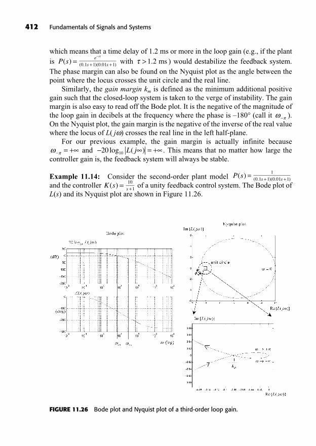
412 Fundamentals of Signals and Systems
which means that a time delay of 1.2 ms or more in the loop gain (e.g., if the plantis with ) would destabilize the feedback system.The phase margin can also be found on the Nyquist plot as the angle between thepoint where the locus crosses the unit circle and the real line.
Similarly, the gain margin km is defined as the minimum additional positivegain such that the closed-loop system is taken to the verge of instability. The gainmargin is also easy to read off the Bode plot. It is the negative of the magnitude ofthe loop gain in decibels at the frequency where the phase is –180° (call it ).On the Nyquist plot, the gain margin is the negative of the inverse of the real valuewhere the locus of L( j ) crosses the real line in the left half-plane.
For our previous example, the gain margin is actually infinite becauseand . This means that no matter how large the
controller gain is, the feedback system will always be stable.
Example 11.14: Consider the second-order plant model and the controller of a unity feedback control system. The Bode plot ofL(s) and its Nyquist plot are shown in Figure 11.26.
s +10
1K s( ) =
s s( . )( . )+ +1
0 1 1 0 01 1P s( ) =
= +20 10log ( )L j= +
>1 2. mse
s s
s
( . )( . )+ +0 1 1 0 01 1P s( ) =
FIGURE 11.26 Bode plot and Nyquist plot of a third-order loop gain.
For this example, the crossover frequency is approximately ,and the frequency where the phase is 180° is approximately .The phase margin is given by
(11.40)
The phase margin is also indicated on the Nyquist plot as the angle between thepoint where the locus crosses the unit circle and the real line.
The gain margin is given by
(11.41)
SUMMARY
In this chapter, we analyzed LTI feedback control systems.
Feedback control has the ability to reject system output disturbances, reducethe effect of uncertainty, and stabilize unstable systems.We distinguished between two types of feedback control systems: regulatorsand tracking systems.Closed-loop stability is a necessary requirement for any feedback system. Wegave four equivalent stability theorems for unity-feedback control systems.We also introduced Routh’s criterion, the root locus, and the Nyquist criterionas different means of assessing closed-loop stability.Two simple measures of closed-loop stability robustness were defined: thegain margin and the phase margin.
TO PROBE FURTHER
Feedback control systems are studied in detail in control engineering texts(Bélanger, 1995; Kuo and Golnaraghi, 2002). For a more theoretical treatment ofcontrol systems, see Doyle, Francis and Tannenbaum, 1992.
EXERCISES
Exercises with Solutions
Exercise 11.1
Consider the causal LTI unity feedback regulator in Figure 11.27, where
, and .k +[ )0,s s
s s( )( )
+ ++ +
2 3 2 9
2 3K s( ) =s
s s s
( )
( )( )+ + +1
1 5 2 252
P s( ) =
k L jm = =20 2210log ( ) dB.
=L j co m( ) .125 55� �
= 33 7. rad/sco = 7 8. rad/s
Application of Transform Techniques to LTI Feedback Control Systems 413
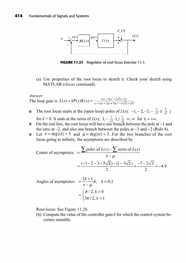
414 Fundamentals of Signals and Systems
(a) Use properties of the root locus to sketch it. Check your sketch usingMATLAB (rlocus command).
Answer:The loop gain is .
The root locus starts at the (open-loop) poles of L(s):
for k = 0. It ends at the zeros of L(s): j for .On the real line, the root locus will have one branch between the pole at 1 andthe zero at 2, and also one branch between the poles at 3 and 2 (Rule 4).Let and . For the two branches of the rootlocus going to infinity, the asymptotes are described by
Center of asymptotes:
Angles of asymptotes:
Root locus: See Figure 11.28.(b) Compute the value of the controller gain k for which the control system be-
comes unstable.
=+
=
===
2 10 1
2 0
3 2 1
kk
k
k
μ, ,
/ ,
/ ,
=
=
poles of zeros of L s L s( ) ( )
(
μ
1 2 3 5 22 1 3 2
2
7 2 2
24 9
) ( ).= =
μ = =deg{ }n 3= =deg{ }d 5
k = +,3
2±3
21,
j5
2±5
21 2 3, , ,
k s s s
s s s
( )( )
( )( )(
+ ++ +
1 3 2 9
1 2
2
++ + +3 5 2 252)( )s sL s kP s K s( ) ( ) ( )= =
FIGURE 11.27 Regulator of root locus Exercise 11.1.
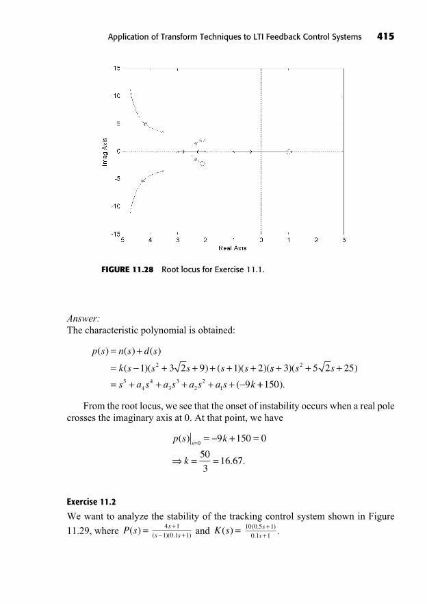
Answer:The characteristic polynomial is obtained:
From the root locus, we see that the onset of instability occurs when a real polecrosses the imaginary axis at 0. At that point, we have
Exercise 11.2
We want to analyze the stability of the tracking control system shown in Figure
11.29, where and .s
s
( . )
.
++
10 0 5 1
0 1 1K s( ) =s
s s( )( . )
++
4 1
1 0 1 1P s( ) =
p s k
k
s( )
. .
= = + =
= =
09 150 0
50
316 67
p s n s d s
k s s s s s
( ) ( ) ( )
( )( ) ( )( )(
= +
= + + + + +1 3 2 9 1 22 ss s s
s a s a s a s a s k
+ + +
= + + + + +
3 5 2 25
9
2
54
43
32
21
)( )
( ++150).
Application of Transform Techniques to LTI Feedback Control Systems 415
FIGURE 11.28 Root locus for Exercise 11.1.
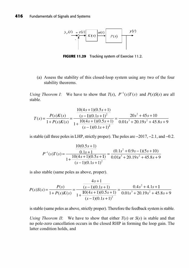
(a) Assess the stability of this closed-loop system using any two of the fourstability theorems.
Using Theorem I: We have to show that T(s), and P(s)S(s) are allstable.
is stable (all three poles in LHP, strictly proper). The poles are 2017, 2.1, and 0.2.
is also stable (same poles as above, proper).
is stable (same poles as above, strictly proper). Therefore the feedback system is stable.
Using Theorem II: We have to show that either T(s) or S(s) is stable and that no pole-zero cancellation occurs in the closed RHP in forming the loop gain. Thelatter condition holds, and
P s S sP s
P s K s
ss s
( ) ( )( )
( ) ( )( )( . )=
+=
++
+1
4 11 0 1 1
1110 4 1 0 5 1
1 0 1 1
0 4 4 1
2
2
( )( . )( )( . )
. .s s
s s
s s+ +
+
=+ +11
0 01 20 19 45 8 93 2. . .s s s+ + +
P s T s
ss
s s=
++
+ + +1
10 0 5 10 1 1
110 4 1 0 5
( ) ( )
( . ).
( )( . 111 0 1 1
0 1 0 9 1 5 10
0 012
2
)( )( . )
( . . )( )
.s s
s s s
+
=+ +
ss s s3 220 19 45 8 9+ + +. .
T sP s K s
P s K s
s ss
( )( ) ( )
( ) ( )
( )( . )(=
+=
+ +
1
10 4 1 0 5 111 0 1 1
110 4 1 0 5 1
1 0 1 1
2)( . )( )( . )
( )( . )
ss s
s s
+
+ + ++ 22
2
3 2
20 45 10
0 01 20 19 45 8 9=
+ ++ + +s s
s s s. . .
P s T s1( ) ( )
416 Fundamentals of Signals and Systems
FIGURE 11.29 Tracking system of Exercise 11.2.
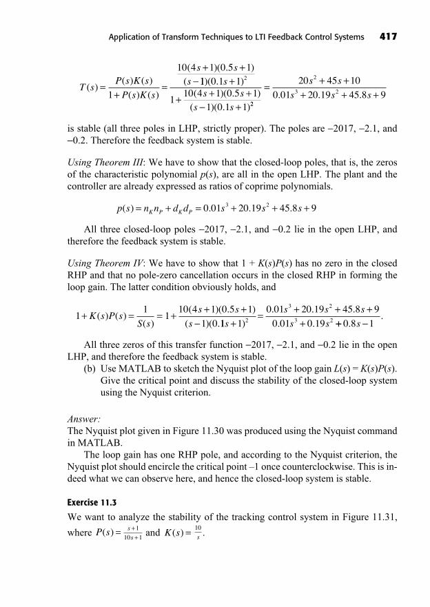
Application of Transform Techniques to LTI Feedback Control Systems 417
is stable (all three poles in LHP, strictly proper). The poles are 2017, 2.1, and 0.2. Therefore the feedback system is stable.
Using Theorem III: We have to show that the closed-loop poles, that is, the zerosof the characteristic polynomial p(s), are all in the open LHP. The plant and thecontroller are already expressed as ratios of coprime polynomials.
All three closed-loop poles 2017, 2.1, and 0.2 lie in the open LHP, andtherefore the feedback system is stable.
Using Theorem IV: We have to show that 1 + K(s)P(s) has no zero in the closedRHP and that no pole-zero cancellation occurs in the closed RHP in forming theloop gain. The latter condition obviously holds, and
All three zeros of this transfer function 2017, 2.1, and 0.2 lie in the openLHP, and therefore the feedback system is stable.
(b) Use MATLAB to sketch the Nyquist plot of the loop gain L(s) = K(s)P(s).Give the critical point and discuss the stability of the closed-loop systemusing the Nyquist criterion.
Answer:The Nyquist plot given in Figure 11.30 was produced using the Nyquist commandin MATLAB.
The loop gain has one RHP pole, and according to the Nyquist criterion, theNyquist plot should encircle the critical point –1 once counterclockwise. This is in-deed what we can observe here, and hence the closed-loop system is stable.
Exercise 11.3
We want to analyze the stability of the tracking control system in Figure 11.31,
where and .s=10
K s( ) =s
s
++1
10 1P s( ) =
11
110 4 1 0 5 1
1 0+ = = +
+ +K s P s
S s
s s
s( ) ( )
( )
( )( . )
( )( .11 1
0 01 20 19 45 8 9
0 01 0 192
3 2
3 2s
s s s
s s+=
+ + ++)
. . .
. . ++ 0 8 1..
s
p s n n d d s s sK P K P( ) . . .= + = + + +0 01 20 19 45 8 93 2
T sP s K s
P s K s
s ss
( )( ) ( )
( ) ( )
( )( . )(=
+=
+ +
1
10 4 1 0 5 111 0 1 1
110 4 1 0 5 1
1 0 1 1
2)( . )( )( . )
( )( . )
ss s
s s
+
+ + ++ 22
2
3 2
20 45 10
0 01 20 19 45 8 9=
+ ++ + +s s
s s s. . .
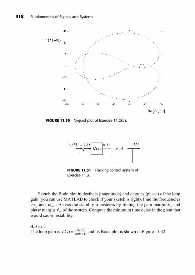
418 Fundamentals of Signals and Systems
FIGURE 11.31 Tracking control system ofExercise 11.3.
FIGURE 11.30 Nyquist plot of Exercise 11.2(b).
Sketch the Bode plot in decibels (magnitude) and degrees (phase) of the loopgain (you can use MATLAB to check if your sketch is right). Find the frequencies
and . Assess the stability robustness by finding the gain margin km andphase margin of the system. Compute the minimum time delay in the plant thatwould cause instability.
Answer:The loop gain is and its Bode plot is shown in Figure 11.32.s
s s
( )
( )
++
10 1
10 1L s( ) =
m
co
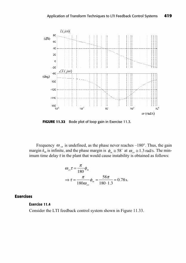
Application of Transform Techniques to LTI Feedback Control Systems 419
FIGURE 11.32 Bode plot of loop gain in Exercise 11.3.
Frequency is undefined, as the phase never reaches –180°. Thus, the gainmargin km is infinite, and the phase margin is at . The min-imum time delay in the plant that would cause instability is obtained as follows:
Exercises
Exercise 11.4
Consider the LTI feedback control system shown in Figure 11.33.
co m
com
=
= = =
180
180
58
180 1 30 78
.. s.
co 1 3. rad/sm 58�

420 Fundamentals of Signals and Systems
The transfer functions of the different causal components of the control system
are , , and .(a) Compute the loop gain L(s) and the closed-loop characteristic polynomial
p(s). Is the closed-loop system stable?
(b) Find the sensitivity S(s) and complementary sensitivity T(s) functions.
(c) Find the steady-state error signal of the closed-loop response y(t) to theinput .
(d) Assume that the real parameter k is an additional gain on the controller;that is, the controller is kK(s). Sketch the root locus for the real parametervarying in .
Exercise 11.5
We want to analyze the stability of the tracking control system shown in Figure
11.34, where and . Assess the stability of this
closed-loop system using any two of the four stability theorems.
s
s
( . )+10 0 5 1K s( ) =s
s s
.
( . )( . )
++ +0 1 1
0 01 1 0 1 1P s( ) =
k +[ )0,
y t td ( ) sin( )=
s
s +1
10 1P s( ) =s
s
++
4 8
10K s( ) =s +
1
1G sa ( ) =
FIGURE 11.34 Feedback control system ofExercise 11.5.
FIGURE 11.33 Feedback control system of Exercise 11.4.
Answer:

Exercise 11.6
Consider the LTI unity feedback regulator in Figure 11.35.
Application of Transform Techniques to LTI Feedback Control Systems 421
FIGURE 11.35 Feedback regulator of Exercise 11.6.
FIGURE 11.36 Feedback control system of Exercise 11.7.
The transfer functions in this regulator are , ,
and . Use properties of the root locus to sketch it. Check your sketchusing MATLAB (rlocus command).
Exercise 11.7
Consider the LTI feedback control system shown in Figure 11.36, where
, , and the plant model P is .(a) Compute the loop gain L(s) and the closed-loop characteristic polynomial
p(s). Is the closed-loop system stable?
(b) Find the sensitivity function S(s) and the complementary sensitivity func-tion T(s).
(c) Find the steady-state error of the closed-loop step response y(t), that is, forthe step reference .
(d) Assume that the real parameter k is an additional gain on the controller,that is, the controller is kK(s). Sketch the root locus for the real parametervarying in .k +[ )0,
y t q td ( ) ( )=
s
s
+ 2P s( ) =s
s
( )
( )
++
100 2 1
1K s( ) =s( )+
10
3
G sa ( ) =
k +[ )0,s +
1
2K s( ) =s s
s s s
( )
( )( )
++ +
2
2
4 4
1 2 1P s( ) =
controller actuator plant

422 Fundamentals of Signals and Systems
Answer:
Exercise 11.8
Sketch the Nyquist plots of the following loop gains. Assess closed-loop stability(use the critical point –1.)
(a)
(b)
Exercise 11.9
We want to analyze the stability of the tracking control system in Figure 11.37,
where and .s
s
( )+1K s( ) =s
s s
.
( )( )
++ +
0 1 1
1 10 1P s( ) =
s s( )( )+1
1 1L s( ) =
s( )+1
1 2L s( ) =
FIGURE 11.37 Feedback control system ofExercise 11.9.
Hand sketch the Bode plot in decibels (magnitude) and degrees (phase) of the loopgain. You can use MATLAB to check if your sketch is right. Find the crossoverfrequency and the frequency where the phase is –180°: . Assess the stability robustness by finding the gain margin km and phase margin of the sys-tem. Compute the minimum time delay in the plant that would cause instability.
Answer:
Exercise 11.10
Sketch the Nyquist plot of the loop gain . Identify the frequencieswhere the locus of L( j ) crosses the unit circle and the real axis (if it does.)
Exercise 11.11
Consider the spacecraft shown in Figure 11.38, which has to maneuver in order todock on a space station.
s
s s( )( )
++ +
2
1 10 1L s( ) =
m
co
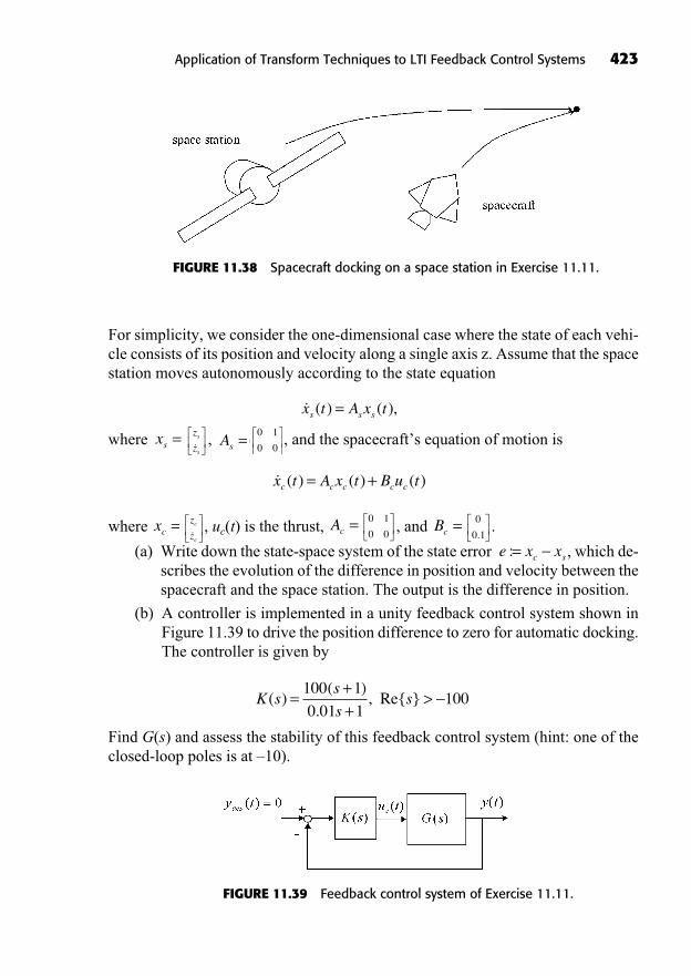
For simplicity, we consider the one-dimensional case where the state of each vehi-cle consists of its position and velocity along a single axis z. Assume that the spacestation moves autonomously according to the state equation
where , , and the spacecraft’s equation of motion is
where , uc(t) is the thrust, , and .
(a) Write down the state-space system of the state error , which de-scribes the evolution of the difference in position and velocity between thespacecraft and the space station. The output is the difference in position.
(b) A controller is implemented in a unity feedback control system shown inFigure 11.39 to drive the position difference to zero for automatic docking.The controller is given by
Find G(s) and assess the stability of this feedback control system (hint: one of theclosed-loop poles is at –10).
K ss
ss( )
( )
., Re{ }=
++
>100 1
0 01 1100
e x xc s:=
0
0 1.Bc =
0 1
0 0Ac =
z
zc
c�xc =
�x t A x t B u tc c c c c( ) ( ) ( )= +
=0 1
0 0As =
z
zs
s�xs =
�x t A x ts s s( ) ( ),=
Application of Transform Techniques to LTI Feedback Control Systems 423
FIGURE 11.38 Spacecraft docking on a space station in Exercise 11.11.
FIGURE 11.39 Feedback control system of Exercise 11.11.
(c) Find the loop gain, sketch its Bode plot, and compute the phase margin of the closed-loop system. Assuming for the moment that the controller wouldbe implemented on Earth, what would be the longest communication delay thatwould not destabilize the automatic docking system?
(d) Compute the sensitivity function of the system and give the steady-state errorto a unit step disturbance on the output.
Answer:
424 Fundamentals of Signals and Systems
425
Discrete-Time FourierSeries and FourierTransform
12
In This Chapter
Response of Discrete-Time LTI Systems to Complex ExponentialsFourier Series Representation of Discrete-Time Periodic SignalsProperties of the Discrete-Time Fourier SeriesDiscrete-Time Fourier TransformProperties of the Discrete-Time Fourier TransformDTFT of Periodic Signals and Step SignalsDualitySummaryTo Probe FurtherExercises
((Lecture 42: Definition of the Discrete-Time Fourier Series))
In this chapter, we go back to the study of discrete-time signals, this time fo-cusing on the frequency domain. We will see that periodic discrete-time signalscan be expanded in a finite Fourier sum of complex harmonics. However, ape-
riodic discrete-time signals require a continuum of complex exponentials to repre-sent them. Thus, the Fourier transform of a discrete-time signal is a continuousfunction of frequency.
426 Fundamentals of Signals and Systems
RESPONSE OF DISCRETE-TIME LTI SYSTEMS TO COMPLEX EXPONENTIALS
Recall that complex exponentials of the type Czn are eigenfunctions of discrete-time linear time-invariant (DLTI) systems; that is, they remain basically invariantunder the action of delays. For example, they are used to find homogeneous re-sponses of difference systems. The response of a DLTI system to a complex expo-nential input is the same complex exponential with only a change in (complex)amplitude: . The complex amplitude factor is in general a func-tion of the complex number z. To show that the complex exponential zn is an eigen-function of a DLTI system, we write,
(12.1)
The system’s response has the form , where ,
assuming that the sum converges. The function H(z) is called the z-transform of theimpulse response of the system. For Fourier analysis, we will restrict our attentionto complex exponentials that have z lying on the unit circle, that is, of the form e j n.
FOURIER SERIES REPRESENTATION OF DISCRETE-TIME PERIODIC SIGNALS
The complex exponential of frequency is periodic with fundamen-
tal period N and fundamental frequency . The set of all discrete-timecomplex exponentials that are periodic with (not necessarily fundamental) periodN is given by
(12.2)
This set of harmonically related complex exponentials is actually redundant, as
there are only N distinct exponentials in it. For example, , so, and in general, for any integer r,
(12.3)k k rN
n n[ ] [ ].= +
1 1[ ] [ ]n n
N= +
e ej
Nn j N
Nn
21
2
=+( )
k
jk n jkN
nn e e k[ ] , , , , , , , .= = =0
2
2 1 0 1 2… …
1=2=N0 :=
2
N1 =e j n1
h k z k[ ]k=
+
H z( ) =y n H z zn[ ] ( )=
y n h k x n k h k z
z h
k
n k
k
n
[ ] [ ] [ ] [ ]
[
= =
=
=
+
=
+
kk z k
k
] .=
+
z h n H z zn n=[ ] ( )
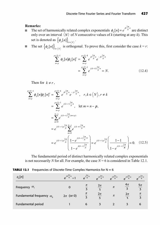
Remarks:The set of harmonically related complex exponentials are distinctonly over an interval of N consecutive values of k (starting at any k). Thisset is denoted as .
The set is orthogonal. To prove this, first consider the case k = r:
(12.4)
Then for ,
(12.5)
The fundamental period of distinct harmonically related complex exponentialsis not necessarily N for all. For example, the case N = 6 is considered in Table 12.1.
k rn p
p Njk
Nn jr
Nn
n p
p N
n n e e[ ] [ ]=
+
=
+
=1 2 211
21
= ==
+
, , ,
,( )
r k N r k
e m nj k r
Nn
n p
p N
let pp
e
e e
j k rN
m p
m
N
j k r pN
j k
,
( ) ( )
( ) (
=
=
+
=
2
0
1
2rr
Nm
m
N
j k r pN
j k rN
N
je
e
e
)
( )( )
2
0
1
22
1
1
=
=(( )
( )
( )k rN
j k r pN
j k re
e
=2
2
2
1 1
1 NN
= 0.
k r
k kn p
p Njk
Nn jk
Nn
n p
p N
n n e e[ ] [ ]=
+
=
+
=1 2 211
21
= ==
+
e Nj k k
Nn
n p
p N( )
.
k k Nn[ ]{ } =
k k Nn[ ]{ } =
Nk
jkN
nn e[ ] =
2
Discrete-Time Fourier Series and Fourier Transform 427
Frequency 0
Fundamental frequency (or 0)
Fundamental period 1 6 3 2 3 6
323
23320
53
43
2331
ej n5
26e
j n426e
j n326e
j n226e
j n26e
j n026 1=k n[ ]
TABLE 12.1 Frequencies of Discrete-Time Complex Harmonics for N = 6
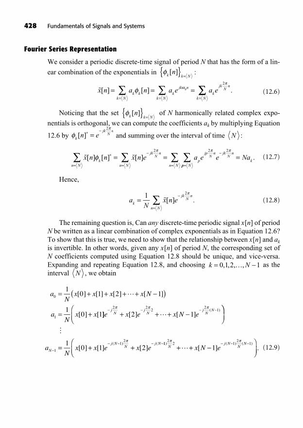
428 Fundamentals of Signals and Systems
Fourier Series Representation
We consider a periodic discrete-time signal of period N that has the form of a lin-
ear combination of the exponentials in :
(12.6)
Noticing that the set of N harmonically related complex expo-
nentials is orthogonal, we can compute the coefficients ak by multiplying Equation
12.6 by and summing over the interval of time :
(12.7)
Hence,
(12.8)
The remaining question is, Can any discrete-time periodic signal x[n] of periodN be written as a linear combination of complex exponentials as in Equation 12.6?To show that this is true, we need to show that the relationship between x[n] and ak
is invertible. In other words, given any x[n] of period N, the corresponding set ofN coefficients computed using Equation 12.8 should be unique, and vice-versa.Expanding and repeating Equation 12.8, and choosing as theinterval , we obtain
(12.9)
aN
x x x x N
aN
x x
0
1
10 1 2 1
10 1
= + + + +( )
= +
[ ] [ ] [ ] [ ]
[ ] [
]] [ ] [ ]( )
e x e x N ejN
jN
jN
N+ + +
2 22
21
2 1
= + +
�
aN
x x e x eN
j NN
j N
1
121
0 1 2[ ] [ ] [ ]( ) ( 11
22 1
21
1) ( ) ( )
[ ] ,Nj N
NN
x N e+ +
Nk N= 0 1 2 1, , , ,…
aN
x n ek
jkN
n
n N
==
1 2
[ ] .
x n n x n e a ek
n N
jkN
n
n Np
jpN
n[ ] [ ] [ ]
= =
= =2 2
pp N
jkN
n
n Nk
e Na==
=2
.
Nk
jkN
nn e[ ] =
2
k k Nn[ ]{ } =
x n a n a e a ek k
k Nk
jk n
k Nk
jkN
n
k N
[ ] [ ]= = == = =
0
2
.
k k Nn[ ]{ } =
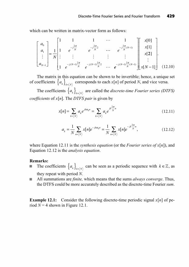
which can be written in matrix-vector form as follows:
(12.10)
The matrix in this equation can be shown to be invertible; hence, a unique setof coefficients corresponds to each x[n] of period N, and vice versa.
The coefficients are called the discrete-time Fourier series (DTFS)
coefficients of x[n]. The DTFS pair is given by
(12.11)
(12.12)
where Equation 12.11 is the synthesis equation (or the Fourier series of x[n]), andEquation 12.12 is the analysis equation.
Remarks:The coefficients can be seen as a periodic sequence with , as
they repeat with period N.All summations are finite, which means that the sums always converge. Thus,the DTFS could be more accurately described as the discrete-time Fourier sum.
Example 12.1: Consider the following discrete-time periodic signal x[n] of pe-riod N = 4 shown in Figure 12.1.
k �ak k N
{ } =
aN
x n eN
x n ek
jk n
n N
jkN
n
n N
= == =
1 10
2
[ ] [ ] ,
x n a e a ek
jk n
k Nk
jkN
n
k N
[ ] = == =
0
2
ak k N
{ } =
ak k N
{ } =
a
a
a
N
e e
N
jN
jN
0
1
1
2 22
1
1 1 1 1
1
�
=
� � � � �
e
e e
jN
N
j NN
j NN
21
12
12
21
( )
( ) ( )ee
x
x
x
j NN
N( ) ( )
[ ]
[ ]
[
12
1
0
1
22
1
]
[ ]
.
�x N
Discrete-Time Fourier Series and Fourier Transform 429
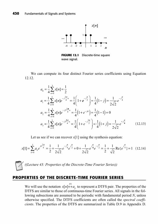
430 Fundamentals of Signals and Systems
We can compute its four distinct Fourier series coefficients using Equation12.12.
(12.13)
Let us see if we can recover x[1] using the synthesis equation:
(12.14)
((Lecture 43: Properties of the Discrete-Time Fourier Series))
PROPERTIES OF THE DISCRETE-TIME FOURIER SERIES
We will use the notation to represent a DTFS pair. The properties of theDTFS are similar to those of continuous-time Fourier series. All signals in the fol-lowing subsections are assumed to be periodic with fundamental period N, unlessotherwise specified. The DTFS coefficients are often called the spectral coeffi-cients. The properties of the DTFS are summarized in Table D.9 in Appendix D.
x n aFS
k[ ]
x a e e e ek
jk
k
j j j[ ]1
1
2
1
2 20
1
2 2
24
0
34 2= = + + +
=
44 2 41
2
1
21e e
j j= + =Re{ }
a x n
a x n e
n
j n
n
00
3
1
24
0
3
1
4
1
2
1
4
1
41
= =
= = +
=
=
[ ]
[ ] ee j e
a x n e
j j
j
= ( ) =
=
2 4
2
22
1
41
1
2 2
1
4[ ] 4
0
3
3
3
1
41
1
41 1 0
1
4
n
n
j
j
e
a x n e
=
= +( ) = ( ) =
= [ ]224
0
3 32
1
41
1
41
1
2 2
n
n
j je j e
=
+= + = +( ) = 44
FIGURE 12.1 Discrete-time squarewave signal.
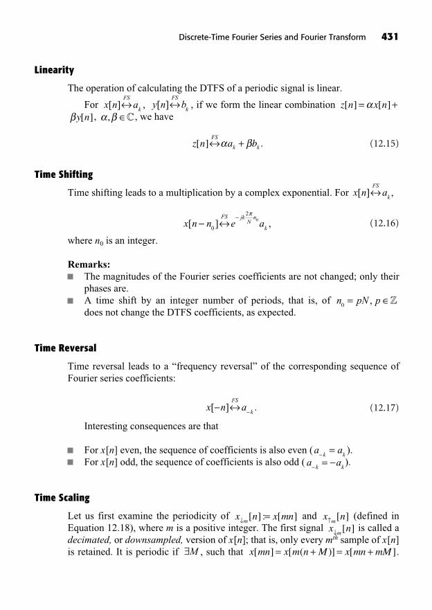
Linearity
The operation of calculating the DTFS of a periodic signal is linear.
For , , if we form the linear combination , , we have
(12.15)
Time Shifting
Time shifting leads to a multiplication by a complex exponential. For ,
(12.16)
where n0 is an integer.
Remarks:The magnitudes of the Fourier series coefficients are not changed; only theirphases are.A time shift by an integer number of periods, that is, of does not change the DTFS coefficients, as expected.
Time Reversal
Time reversal leads to a “frequency reversal” of the corresponding sequence ofFourier series coefficients:
(12.17)
Interesting consequences are that
For x[n] even, the sequence of coefficients is also even ( ).For x[n] odd, the sequence of coefficients is also odd ( ).
Time Scaling
Let us first examine the periodicity of and (defined inEquation 12.18), where m is a positive integer. The first signal is called adecimated, or downsampled, version of x[n]; that is, only every mth sample of x[n]is retained. It is periodic if , such that .x mn x m n M x mn mM[ ] [ ( )] [ ]= + = +M
x nm[ ]
x nm[ ]x n x mn
m=[ ] : [ ]
a ak k=
a ak k=
x n aFS
k[ ] .
n pN p0= , �
x n n e aFS jk
Nn
k[ ] ,
0
20
x n aFS
k[ ]
z n a bFS
k k[ ] .+
, �y n[ ]z n x n[ ] [ ]= +y n b
FS
k[ ]x n a
FS
k[ ]
Discrete-Time Fourier Series and Fourier Transform 431
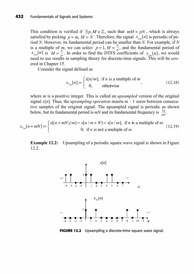
This condition is verified if , such that , which is alwayssatisfied by picking . Therefore, the signal is periodic of pe-riod N. However, its fundamental period can be smaller than N. For example, if Nis a multiple of m, we can select , and the fundamental period of
is . In order to find the DTFS coefficients of , we wouldneed to use results in sampling theory for discrete-time signals. This will be cov-ered in Chapter 15.
Consider the signal defined as
(12.18)
where m is a positive integer. This is called an upsampled version of the originalsignal x[n]. Thus, the upsampling operation inserts m – 1 zeros between consecu-tive samples of the original signal. The upsampled signal is periodic as shownbelow, but its fundamental period is mN and its fundamental frequency is .
(12.19)
Example 12.2: Upsampling of a periodic square wave signal is shown in Figure12.2.
x n mNx n mN m x n m N x n m n
m+ =
+ = + =[ ] :
[( ) ] [ / ] [ / ], if iis a multiple of
if is not a multiple
m
n0, of m
2
mN
x nx n m n m
m=[ ] :
[ ],
,
if is a multiple of
othe0 rrwise,
x nm[ ]
N
m=M =x n
m[ ]
N
mp M= =1,
x nm[ ]p m M N= =,
mM pN=p M, Z
432 Fundamentals of Signals and Systems
FIGURE 12.2 Upsampling a discrete-time square wave signal.
The Fourier series coefficients of the upsampled signal are given by
(12.20)
where is viewed as a periodic sequence of period mN.
Proof:
(12.21)
Periodic Convolution of Two Signals
Suppose that x[n] and y[n] are both periodic with period N. For ,
, we have
(12.22)
Remarks:The periodic convolution is itself periodic of period N (show it as an exercise).What is the use of a periodic convolution? It is useful in periodic signal filter-ing. The DTFS coefficients of the input signal are the ak’s, and the bk’s are cho-sen by the filter designer to attenuate or amplify certain frequencies. Theresulting discrete-time output signal is given by the periodic convolutionabove. But it is mostly useful for convolving signals of finite support: with suf-ficient zero-padding, we can pretend that each one of the zero-padded signalsrepresents a period of a periodic signal and use Equation 12.22 to compute theconvolution in the frequency domain. The zero padding has the effect of turn-ing the periodic convolution into an ordinary convolution. We can then obtainthe corresponding time-domain signal by solving Equation 12.10. This idealeads to the discrete Fourier transform (DFT) and the fast Fourier transform(FFT) algorithm, which are widely used techniques although beyond the scopeof this book.
x m y n m Na bm N
FS
k k[ ] [ ] .=
y n bFS
k[ ]
x n aFS
k[ ]
bmN
x n emN
x n m ek m
jkmN
n
n mN
jkmN= =
=
1 12 2
[ ] [ ]nn
n m m N
jkNp
p NkmN
x p ema
=
=
= =
0 1
21 1
, ,.., ( )
[ ]
1m ka{ }
x nma
m
FS
k[ ] ,1
x nm[ ]
Discrete-Time Fourier Series and Fourier Transform 433

Multiplication of Two Signals
The time domain multiplication of the two signals defined earlier yields
(12.23)
that is, a periodic convolution of the two sequences of spectral coefficients. Thisproperty is used in discrete-time modulation of a periodic signal.
First Difference
The first difference of a periodic signal (often used as an approximation to thecontinuous-time derivative) has the following spectral coefficients:
(12.24)
Running Sum
The running sum of a signal is the inverse of the first difference “system.” Note thatthe running sum of a periodic signal is periodic if and only if a0 = 0; that is, the DCcomponent of the signal is 0. In this case,
(12.25)
Conjugation and Conjugate Symmetry
The complex conjugate of a periodic signal yields complex conjugation and fre-quency reversal of the spectral coefficients:
(12.26)
Interesting consequences are that
For x[n] real, the sequence of coefficients is conjugate symmetric ( ).This implies
.For x[n] real and even, the sequence of coefficients is also real and even( ).a ak k= �
Im{{ } Im{ }a ak k=a a a a a a ak k k k k k= = =, ( ) ( ), , Re{ } Re{ },0 �
a ak k=
x n aFS
k[ ]
x m
e
am
n FS
jkN
k[ ]
( )
.=
1
12
x n x n e aFS jk
Nk
[ ] [ ] ( ) .1 12
x n y n a bFS
l k ll N
[ ] [ ] ,=
434 Fundamentals of Signals and Systems
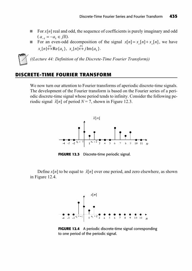
Discrete-Time Fourier Series and Fourier Transform 435
For x[n] real and odd, the sequence of coefficients is purely imaginary and odd( ).For an even-odd decomposition of the signal , we have
.
((Lecture 44: Definition of the Discrete-Time Fourier Transform))
DISCRETE-TIME FOURIER TRANSFORM
We now turn our attention to Fourier transforms of aperiodic discrete-time signals.The development of the Fourier transform is based on the Fourier series of a peri-odic discrete-time signal whose period tends to infinity. Consider the following pe-riodic signal of period N = 7, shown in Figure 12.3. x n[ ]
x n a x n j ae
FS
k o
FS
k[ ] Re{ }, [ ] Im{ }
x n x n x ne o
[ ] [ ] [ ]= +a a jk k= �
FIGURE 12.3 Discrete-time periodic signal.
Define x[n] to be equal to over one period, and zero elsewhere, as shownin Figure 12.4.
x n[ ]
FIGURE 12.4 A periodic discrete-time signal correspondingto one period of the periodic signal.
Let us examine the DTFS pair of given by
(12.27)
(12.28)
Referring to Figure 12.4, if we pick the summation interval such that, we can substitute x[n] for in Equation 12.6:
(12.29)
Define the function
(12.30)
We see that the DTFS coefficients ak are scaled samples of this continuousfunction of frequency . That is,
(12.31)
Using this expression for ak in Equation 12.27, we obtain
(12.32)
At the limit, as in Equation 12.32, we get
.
.The summation over small frequency intervals of width tends to an integral over a frequency interval of width 2 .
Then Equation 12.32 becomes
(12.33)x n X e e dj j n[ ] ( ) ,=1
2 2
x n x n[ ] [ ].
d2
N0=N
k0
0d
N +
x nN
X e e X e ejk jk n
k N
jk jk[ ] ( ) ( )= ==
1 1
20 0 0 0nn
k N0
=
.
aN
X eN
X ek
jN
k j k= =1 12
0( ) ( ).
X e x n ej j n
n
( ) : [ ] .==
+
aN
x n eN
x n ek
jkN
n
n N
jkN
n
n
= == =
+1 12 2
[ ] [ ] ..
x n[ ]n n n N1 2
aN
x n ek
jkN
n
n N
==
1 2
[ ] .
x n a ek
jkN
n
k N
[ ] ,==
2
x n[ ]
436 Fundamentals of Signals and Systems
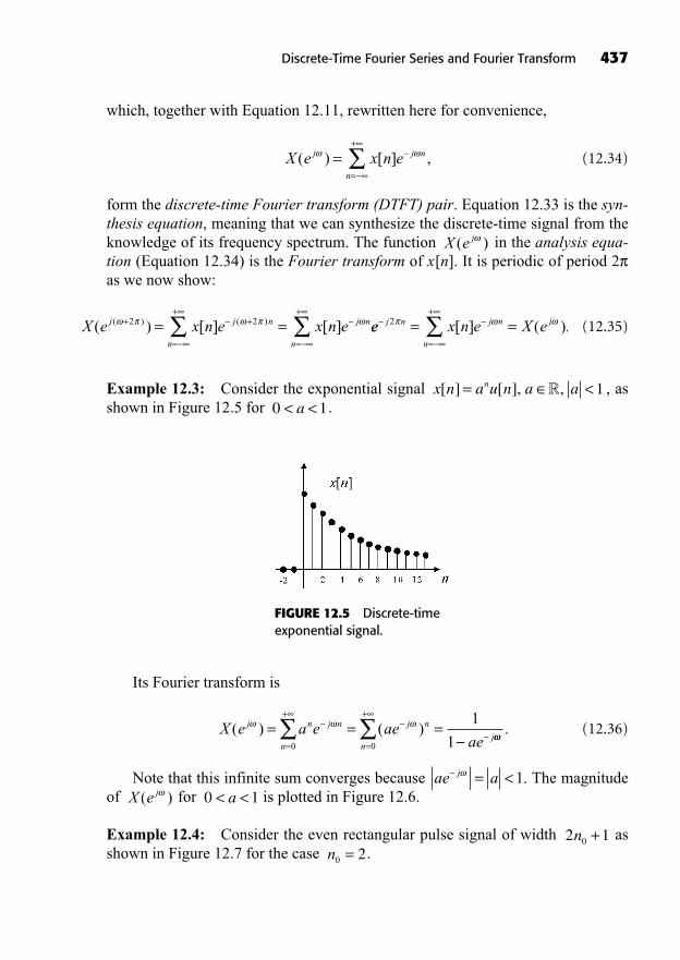
Discrete-Time Fourier Series and Fourier Transform 437
which, together with Equation 12.11, rewritten here for convenience,
(12.34)
form the discrete-time Fourier transform (DTFT) pair. Equation 12.33 is the syn-thesis equation, meaning that we can synthesize the discrete-time signal from theknowledge of its frequency spectrum. The function in the analysis equa-tion (Equation 12.34) is the Fourier transform of x[n]. It is periodic of period 2as we now show:
(12.35)
Example 12.3: Consider the exponential signal , asshown in Figure 12.5 for .0 1< <a
x n a u n a an[ ] [ ], ,= <� 1
X e x n e x n ej j n
n
j n( ) [ ] [ ]( ) ( )+ +
=
+
= =2 2 ee x n e X ej n
n
j n
n
j
=
+
=
+
= =2 [ ] ( ).
X e j( )
X e x n ej j n
n
( ) [ ] ,==
+
FIGURE 12.5 Discrete-timeexponential signal.
Its Fourier transform is
(12.36)
Note that this infinite sum converges because . The magnitudeof for is plotted in Figure 12.6.
Example 12.4: Consider the even rectangular pulse signal of width asshown in Figure 12.7 for the case .n0 2=
2 10n +
0 1< <aX e j( )ae aj = <1
X e a e aeae
j n j n
n
j n
nj
( ) ( )= = ==
+
=
+
0 0
1
1.
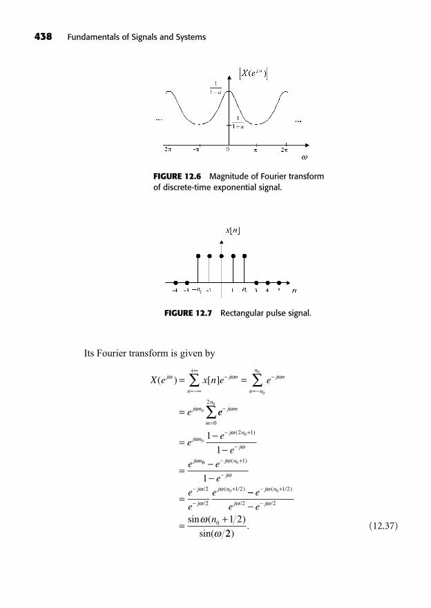
438 Fundamentals of Signals and Systems
FIGURE 12.6 Magnitude of Fourier transformof discrete-time exponential signal.
FIGURE 12.7 Rectangular pulse signal.
Its Fourier transform is given by
(12.37)
X e x n e e
e
j j n
n
j n
n n
n
j n
( ) [ ]= =
=
=
+
= 0
0
0 ee
ee
e
e
j m
m
n
j nj n
j
j n
=+
=
=
0
2
2 1
0
0
01
1
( )
00 0
0
1
2
2
1 2
1
=
+
+
e
e
e
e
e
j n
j
j
j
j n
( )
/
/
( / )
=+
+e
e en
j n
j j
( / )
/ /
sin ( )
sin(
0 1 2
2 2
0 1 2
22).
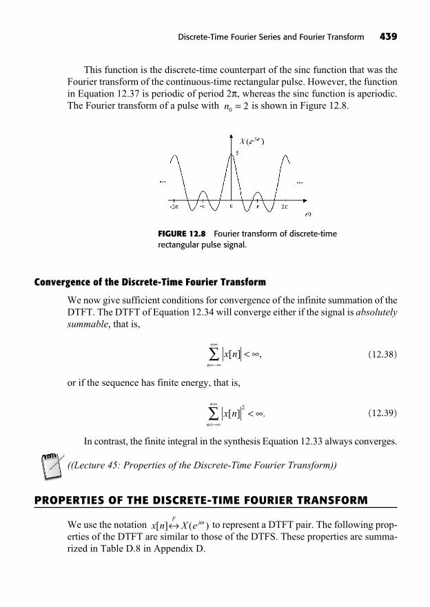
This function is the discrete-time counterpart of the sinc function that was theFourier transform of the continuous-time rectangular pulse. However, the functionin Equation 12.37 is periodic of period 2 , whereas the sinc function is aperiodic.The Fourier transform of a pulse with is shown in Figure 12.8.n0 2=
Discrete-Time Fourier Series and Fourier Transform 439
FIGURE 12.8 Fourier transform of discrete-timerectangular pulse signal.
Convergence of the Discrete-Time Fourier Transform
We now give sufficient conditions for convergence of the infinite summation of theDTFT. The DTFT of Equation 12.34 will converge either if the signal is absolutelysummable, that is,
(12.38)
or if the sequence has finite energy, that is,
(12.39)
In contrast, the finite integral in the synthesis Equation 12.33 always converges.
((Lecture 45: Properties of the Discrete-Time Fourier Transform))
PROPERTIES OF THE DISCRETE-TIME FOURIER TRANSFORM
We use the notation to represent a DTFT pair. The following prop-erties of the DTFT are similar to those of the DTFS. These properties are summa-rized in Table D.8 in Appendix D.
x n X eF
j[ ] ( )
x nn
[ ] .2
=
+
<
x nn
[ ] ,=
+
<
Linearity
The operation of calculating the DTFT of a signal is linear. For ,
, if we form the linear combination , ,then we have:
(12.40)
Time Shifting
Time shifting the signal by leads to a multiplication of the Fourier trans-form by a complex exponential:
(12.41)
Remark: Only the phase of the DTFT is changed.
Frequency Shifting
A frequency shift by leads to a multiplication of x[n] by a complexexponential:
(12.42)
Time Reversal
Time reversal leads to a frequency reversal of the corresponding DTFT:
(12.43)
Proof:
(12.44)
Consequences: For x[n] even, is also even; for x[n] odd, is alsoodd.
X e j( )X e j( )
x n e x m e X ej n
n
j m
m
j[ ] [ ] ( )= ==
+
=
x n X eF j[ ] ( ).
e x n X ej n F j0 0[ ] ( ).( )
0 �
x n n e X eF j n j[ ] ( ).
00
n0 �
z n aX e bY eF j j[ ] ( ) ( ).+
a b, �z n ax n by n[ ] [ ] [ ]= +y n Y eF
j[ ] ( )
x n X eF
j[ ] ( )
440 Fundamentals of Signals and Systems
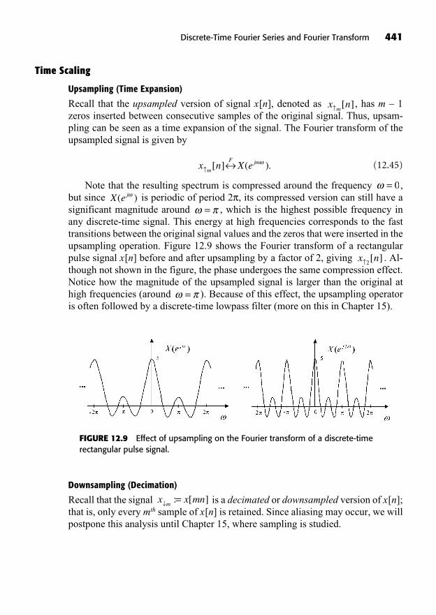
Discrete-Time Fourier Series and Fourier Transform 441
Time Scaling
Upsampling (Time Expansion)
Recall that the upsampled version of signal x[n], denoted as , has m – 1zeros inserted between consecutive samples of the original signal. Thus, upsam-pling can be seen as a time expansion of the signal. The Fourier transform of theupsampled signal is given by
(12.45)
Note that the resulting spectrum is compressed around the frequency ,but since is periodic of period 2 , its compressed version can still have asignificant magnitude around , which is the highest possible frequency inany discrete-time signal. This energy at high frequencies corresponds to the fasttransitions between the original signal values and the zeros that were inserted in theupsampling operation. Figure 12.9 shows the Fourier transform of a rectangularpulse signal x[n] before and after upsampling by a factor of 2, giving . Al-though not shown in the figure, the phase undergoes the same compression effect.Notice how the magnitude of the upsampled signal is larger than the original athigh frequencies (around ). Because of this effect, the upsampling operatoris often followed by a discrete-time lowpass filter (more on this in Chapter 15).
=
x n2[ ]
=X ej( )
= 0
x n X em
F jm[ ] ( ).
x nm[ ]
FIGURE 12.9 Effect of upsampling on the Fourier transform of a discrete-timerectangular pulse signal.
Downsampling (Decimation)
Recall that the signal is a decimated or downsampled version of x[n];that is, only every mth sample of x[n] is retained. Since aliasing may occur, we willpostpone this analysis until Chapter 15, where sampling is studied.
x x mnm=: [ ]
Differentiation in Frequency
Differentiation of the DTFT with respect to frequency gives a multiplication of thesignal by n:
(12.46)
Convolution of Two Signals
For , , we have
(12.47)
Proof: Under the appropriate assumption of convergence, to be able to interchangethe order of summations, we have
(12.48)
Remarks:The basic use of this property is to compute the output signal of a system for aparticular input signal, given its impulse response or DTFT.The convolution property is also useful in discrete-time filter design and feed-back controller design.
Example 12.5: Given a system with and an input, the DTFT of the output is given by
(12.49)Y e H e X ee e
j j jj j( ) ( ) ( )
. ..= =
+1
1 0 8
1
1 0 5
x n u nn[ ] ( . ) [ ]= 0 5h n u nn[ ] ( . ) [ ]= 0 8
x m y n m e x m y n mm
j n
n n
[ ] [ ] [ ] [ ]===
+
==
+
=
+
=
=
e
x m y p e
j n
m
p
j p m
m
[ ] [ ] ( )++
==
+
=
=
x m e y p e
X e
j m
p
j p
m
j
[ ] [ ]
( )YY e j( ).
x m y n m X e Y em
Fj j[ ] [ ] ( ) ( ).
=
y n Y eF
j[ ] ( )x n X eF
j[ ] ( )
nx n jdX e
d
F j
[ ]( )
.
442 Fundamentals of Signals and Systems

We perform a partial fraction expansion of to be able to use Table D.7in Appendix D to obtain y[n]. Note that the first-order terms in the partial fraction
expansion should have the form , not , which usually leads to a wrongsolution. Let for convenience.
(12.50)
(12.51)
(12.52)
Finally, we use Table D.7 to get
(12.53)
Multiplication of Two Signals
With the two signals as defined above,
(12.54)
Remarks:Note that the resulting DTFT is a periodic convolution of the two DTFTs.This property is used in discrete-time modulation and sampling.
First Difference
The first difference of a signal has the following spectrum:
(12.55)x n x n e X eF
j j[ ] [ ] ( ) ( ).1 1
x n y n X e Y e dF
j j[ ] [ ] ( ) ( ) .( )1
2 2
y n u n u nn n[ ] ( . ) [ ] ( . ) [ ].= +8
130 8
5
130 5
1
1 0 8
1 0 5
1 0 810 5
1
1
0 5( . )
( . )
.. .
+= +
+= =zB
A z
zz z
=+
=B1
10 80 5
5
13(..
)
1
1 0 5
1 0 8
1 0 510 8
1
1
0( . )
( . )
..
= ++
= =zA
B z
zz z .. (
..
)8
1
10 50 8
8
13= =A
1
1 0 8 1 0 5 1 0 8 1 0 51 1 1 1( . )( . ) . .+=
++
z z
A
z
B
z
z e j=
A
e aj
A
ae j1
Y e j( )
Discrete-Time Fourier Series and Fourier Transform 443
Running Sum (Accumulation)
The running sum of a signal is the inverse of the first difference:
(12.56)
The frequency-domain impulses at DC account for the possibility that signalx[n] has a nonzero DC component .
Conjugation and Conjugate Symmetry
Taking the conjugate of a signal has the effect of conjugation and frequency re-versal of the DTFT:
(12.57)
Interesting consequences are that
For x[n] real, the DTFT is conjugate symmetric: . This implies
For x[n] real and even, the DTFT is also real and even: .For x[n] real and odd, the DTFT is purely imaginary and odd:
.For an even-odd decomposition of the signal ,
, .
Parseval Equality and Energy Density Spectrum
The Parseval equality establishes a correspondence between the energy of the sig-nal and the energy in its spectrum:
(12.58)
The squared magnitude of the DTFT is referred to as the energy-density spectrum of the signal .
((Lecture 46: DTFT of Periodic and Step Signals, Duality))
x n[ ]X e j( )
2
x n X e dn
j[ ] ( ) .2 2
2
1
2=
+
=
x n j X eo
F j[ ] Im{ ( )}x n X ee
F j[ ] Re{ ( )}
x n x n x ne o
[ ] [ ] [ ]= +X e X e jj j( ) ( )= �
X e X ej j( ) ( )= �
X e X e X ej j j( ) ( ) , ( )= = (even magnitude) XX e X e
X e
j j
j
( ) , ( ) ,
Re{ ( )} Re
(odd phase) 0
=
�
{{ ( )} , Im{ ( )} Im{ ( )}X e X e X ej j j (even) (o= ddd)
X e X ej j( ) ( )=
x n X eF
j[ ] ( ).
X ej( )0 0
x me
X e X e km
nF
jj j[ ]
( )( ) ( ) ( )
=
+1
120
kk=
+
.
444 Fundamentals of Signals and Systems
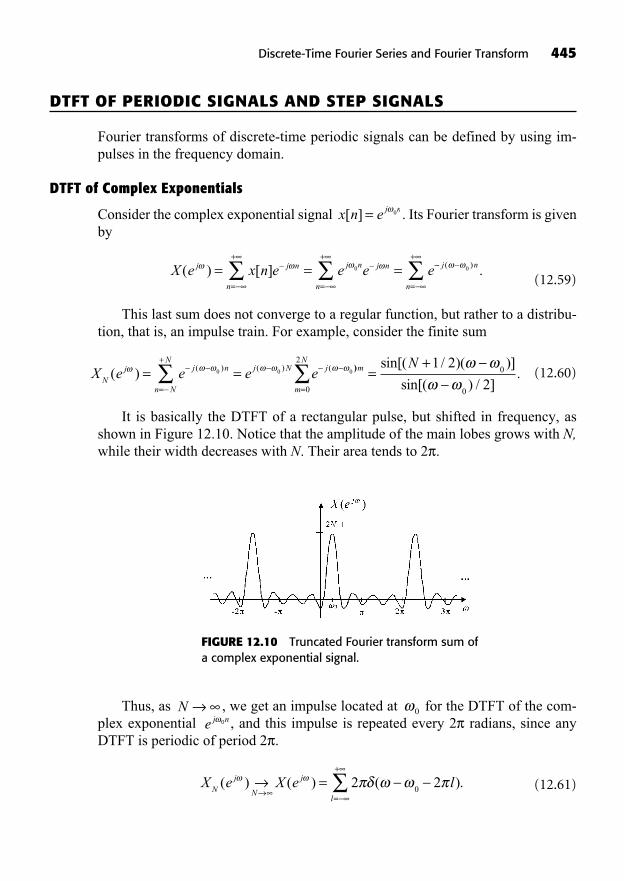
FIGURE 12.10 Truncated Fourier transform sum ofa complex exponential signal.
Thus, as , we get an impulse located at for the DTFT of the com-plex exponential , and this impulse is repeated every 2 radians, since anyDTFT is periodic of period 2 .
(12.61)X e X e lN
j
N
j
l
( ) ( ) ( ).==
+
2 20
e j n0
0N
DTFT OF PERIODIC SIGNALS AND STEP SIGNALS
Fourier transforms of discrete-time periodic signals can be defined by using im-pulses in the frequency domain.
DTFT of Complex Exponentials
Consider the complex exponential signal . Its Fourier transform is givenby
(12.59)
This last sum does not converge to a regular function, but rather to a distribu-tion, that is, an impulse train. For example, consider the finite sum
(12.60)
It is basically the DTFT of a rectangular pulse, but shifted in frequency, asshown in Figure 12.10. Notice that the amplitude of the main lobes grows with N,while their width decreases with N. Their area tends to 2 .
X e e e eN
j j n
n N
Nj N j( ) ( ) ( ) (= =
=
+0 0 0 )) sin[( / )( )]
sin[( ) / ].m
m
N N
=
=+
0
20
0
1 2
2
X e x n e e e ej j n
n
j n j n
n
( ) [ ]= = ==
+
=
+0
=
+j n
n
( ) .0
x n e j n[ ] = 0
Discrete-Time Fourier Series and Fourier Transform 445

446 Fundamentals of Signals and Systems
Check: Inverse Fourier transform. Note that there is only one impulse per inter-val of width 2 .
(12.62)
DTFT of the Step Signal
Since the constant signal x[n] = 1 can be written as , it follows that itsDTFT in the interval is an impulse located at . Thus,
(12.63)
In order to find the Fourier transform of the unit step u[n], for which the analy-sis Equation 12.34 does not converge, we write this signal as the limit of twoexponential signals pieced together at the origin plus the constant , as shown inFigure 12.11:
(12.64)u n u n u nn n[ ] lim [ ( )] [ ]( )= + + ++1
2
1
21
1
21
1 .
1 2
x n lF
l
[ ] ( ).==
+
1 2 2
= 0[ , ]x n e j n[ ] = 0
x n l e d ej n
l
j n[ ] ( )= ==
+1
22 2
02
0
FIGURE 12.11 Piecewise exponential signal tending to the unit step.
We already know that the DTFT of is , and by the time
reversal and time shifting properties, we have – . 1
2 1
j
j
e
e++ 11( ) [ ( )]n F
u n1
2
1
2
1
1 e jnu n[ ]1
2
Taking the Fourier transform of the right-hand side of Equation 12.64 before tak-ing the limit, we obtain
(12.65)
Hence, the Fourier transform of the unit step is given by
.
From the Fourier Series to the Fourier Transform
Recall that a periodic signal of fundamental period N can be represented as aFourier series as follows:
(12.66)
Using the DTFT formula and the above result, we obtain
(12.67)
X e a e e
a e
jk
jkN
n
k N
j n
n
k
j k
( )
(
=
=
==
2
2NN
n
nk N
klk N
a kN
l
)
( )
==
==
=
=
22
2
222
a kNk
k
( ).=
x n a e a ek
jk n
k Nk
jkN
n
k N
[ ] .= == =
0
2
k( )2k=
++
e j
1
1u n
F[ ]
U e le
ej
l
j
j( ) ( ) lim= + +=
+
21
2 11
11
2
1
1
21
2 1= +
=
+
e
l
j
l
( ) lim+e e e
e e
j j j
j j
( ) ( )
( )( )
1 1
1 1
= ++ +
=
+
( ) lim( ) ( )
21
2
1 11
le
l
j
( )( )
( )
1 1
2= +=
+
e e
l
j j
l
11
2
2 1
1 1
2
( )
( )( )
( )=
e
e e
l
j
j j
l==
+
+1
1 e j .
Discrete-Time Fourier Series and Fourier Transform 447

Thus, we can write the DTFT of a periodic signal by inspection from theknowledge of its Fourier series coefficients (recall that they are periodic).
Example 12.6: Let us find the DTFT of . We firsthave to determine whether this signal is periodic. The sine term repeats every threetime steps, whereas the cosine term repeats every seven time steps. Thus, the sig-nal is periodic of fundamental period N = 21. Write
(12.68)
The nonzero DTFS coefficients of the signal are ,
; hence we have
(12.69)
DTFT of a Periodic Discrete-Time Impulse Train
Let us now find the DTFT of the discrete-time impulse train .
This signal is periodic of period N. Its DTFS coefficients are given by
(12.70)
and hence, the DTFT of the impulse train is simply a train of impulses in the fre-quency domain, equally spaced by radians.
(12.71)
This transform is shown in Figure 12.12.
X eN
kN
l
N
j
lk
N
( ) ( )
(
=
=
==
2 22
20
1
=
kNk
2)
2
N
aN
x n eN
n ek
jkN
n
n
Njk
Nn
n
N
= == =
1 12
0
1 2
0
[ ] [ ] =1 1
N,
n kN[ ]k=
x n[ ] =
X e a k ljklk
( ) ( )=
= +
==
22
212
1
10
10
( ) ( )+ +
+
= =
6
212
6
212l l
j
l l
( ) ( )+= =
14
212
14
212l j l
l l
= + + + + +16
212
6
212
1( ) ( ) (l l j
44
212
14
212
=
l j ll
) ( ) .
1
2a a3 3= =
1
2a j7 =,1
2a a j0 71= =,
x nje e ej n j n j
[ ] = +11
2
1
2
2 721
2 721
2 3211
2 321
n j ne+ .
x n n n[ ] sin( ) cos( )= +1 23
27
448 Fundamentals of Signals and Systems
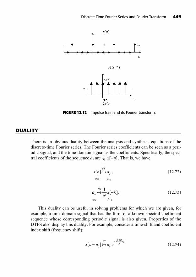
Discrete-Time Fourier Series and Fourier Transform 449
DUALITY
There is an obvious duality between the analysis and synthesis equations of thediscrete-time Fourier series. The Fourier series coefficients can be seen as a peri-odic signal, and the time-domain signal as the coefficients. Specifically, the spec-tral coefficients of the sequence ak are . That is, we have
(12.72)
(12.73)
This duality can be useful in solving problems for which we are given, forexample, a time-domain signal that has the form of a known spectral coefficientsequence whose corresponding periodic signal is also given. Properties of theDTFS also display this duality. For example, consider a time-shift and coefficientindex shift (frequency shift):
(12.74)x n n a eFS
k
jk
Nn
[ ]0
20
aN
x kn
time
FS
freq
1[ ].
x n atime
FS
k
freq
[ ] ,
x n[ ]1
N
FIGURE 12.12 Impulse train and its Fourier transform.
(12.75)
There is no such duality for the DTFT since it is continuous, whereas the sig-nal is discrete.
SUMMARY
This chapter introduced Fourier analysis for discrete-time signals.
Periodic discrete-time signals of fundamental period N have a Fourier seriesrepresentation, where the series is a finite sum of N complex harmonics.Many aperiodic discrete-time signals have a Fourier transform representation,for instance the class of finite-energy signals. The discrete-time Fourier trans-form is typically a continuous function of frequency, and it is always periodicof period 2 radians.The inverse discrete-time Fourier transform is given by an integral over oneperiod of 2 radians. If the DTFT is a rational function of , then a partialfraction expansion approach can be used to get the time-domain signal.The DTFT of a periodic discrete-time signal can be defined with the help offrequency-domain impulses.
TO PROBE FURTHER
For more details on Fourier analysis of discrete-time signals, see Oppenheim,Schafer and Buck, 1999.
EXERCISES
Exercises with Solutions
Exercises 12.1
Compute the Fourier series coefficients {ak} of the signal x[n] shown in Figure12.13. Sketch the magnitude and phase of the coefficients. Write x[n] as a Fourierseries.
e j
e x n ajm
Nn FS
k m
2
[ ] .
450 Fundamentals of Signals and Systems
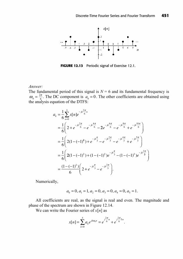
Discrete-Time Fourier Series and Fourier Transform 451
Answer:The fundamental period of this signal is N = 6 and its fundamental frequency is
. The DC component is . The other coefficients are obtained usingthe analysis equation of the DTFS:
Numerically,
All coefficients are real, as the signal is real and even. The magnitude andphase of the spectrum are shown in Figure 12.14.
We can write the Fourier series of x[n] as
x n a e e ekjk n
k
j n j n[ ] .= = +
=
0
0
5 26
26
5
a a a a a a0 1 2 3 4 50 1 0 0 0 1= = = = = =, , , , , .
a x n e
e e
k
jk n
n
jk jk
=
= +
=
1
6
1
62
26
0
5
26
46
[ ]
22
1
62 1 1
66
86
106e e e
jk jk jk+
= ( ( )kkjk jk jk jk
e e e e)+ +
=
323
43
53
1
622 1 1 1 1 1 13
2
( ( ) ) ( ( ) ) ( ( ) )+k k jk k jke e 33
323
1 1
62= +
( ( ) ).
kjk jk
e e
a0
0=2
60=
FIGURE 12.13 Periodic signal of Exercise 12.1.
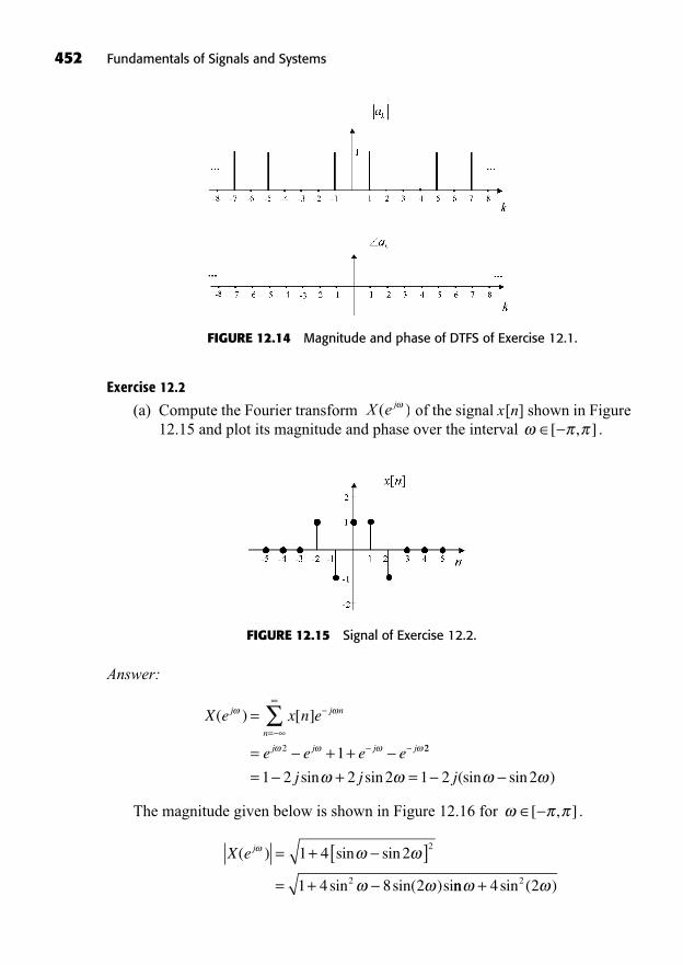
452 Fundamentals of Signals and Systems
Exercise 12.2
(a) Compute the Fourier transform of the signal x[n] shown in Figure12.15 and plot its magnitude and phase over the interval .[ , ]
X e j( )
FIGURE 12.14 Magnitude and phase of DTFS of Exercise 12.1.
FIGURE 12.15 Signal of Exercise 12.2.
Answer:
The magnitude given below is shown in Figure 12.16 for .
X ej( ) sin sin
sin sin( )si
= + [ ]= +
1 4 2
1 4 8 2
2
2 nn sin ( )+ 4 22
[ , ]
X e x n e
e e e e
j j n
n
j j j j
( ) [ ]=
= + +=
2 1 22
1 2 2 2 1 2 2= + =j j jsin sin (sin sin )

Discrete-Time Fourier Series and Fourier Transform 453
FIGURE 12.16 Magnitude of DTFT of Exercise 12.2.
The phase is given by
and is plotted in Figure 12.17 for .[ , ]
=X ej( ) arctansin( ) sin2 2 2
1
FIGURE 12.17 Phase of DTFT of Exercise 12.2.
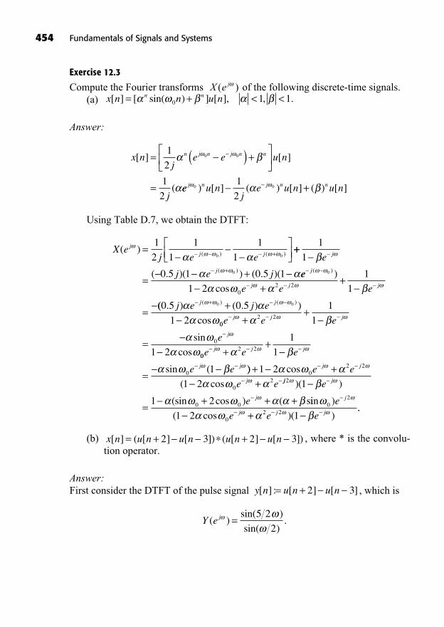
Exercise 12.3
Compute the Fourier transforms of the following discrete-time signals.(a)
Answer:
Using Table D.7, we obtain the DTFT:
(b) , where * is the convolu-tion operator.
Answer:First consider the DTFT of the pulse signal , which is
Y e j( )sin( )
sin( ).=
5 2
2
y n u n u n[ ] : [ ] [ ]= + 2 3
x n u n u n u n u n[ ] ( [ ] [ ]) ( [ ] [ ])= + +2 3 2 3
X ej e e
jj j( ) ( ) ( )= +
1
2
1
1
1
10 0++
=++
1
1
0 5 1 0 5 10
e
j e j
j
j( . )( ) ( . )(( ) ee
e e e
j
j j j++
=
( ) )
cos
0
1 2
1
102 2
(( . ) ( . ) )
cos
( ) ( )0 5 0 5
1 2
0 0j e j ej j+ +
002 2
0
1
1
1 2
e e e
e
j j j
j
++
=sin
cos 002 2
0
1
1
1
e e e
e e
j j j
j j
++
=sin ( )) cos
( cos
+ ++1 2
1 20
2 2
02
e e
e e
j j
j jj j
j
e
e
2
0 0
1
1 2
)( )
(sin cos ) ( s=
+ + + iin )
( cos )( )0
2
02 21 2 1
e
e e e
j
j j j+..
x nj
e e u n
j
n j n j n n[ ] [ ]
(
= ( ) +
=
1
2
1
2
0 0
ee u nj
e u n u nj n j n n0 01
2) [ ] ( ) [ ] ( ) [ ]+
x n n u nn n[ ] [ sin( ) ] [ ], , .= + < <0 1 1X e j( )
454 Fundamentals of Signals and Systems
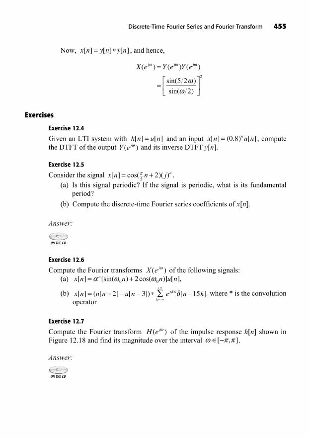
Discrete-Time Fourier Series and Fourier Transform 455
Now, , and hence,
Exercises
Exercise 12.4
Given an LTI system with and an input , computethe DTFT of the output and its inverse DTFT y[n].
Exercise 12.5
Consider the signal .(a) Is this signal periodic? If the signal is periodic, what is its fundamental
period?
(b) Compute the discrete-time Fourier series coefficients of x[n].
Answer:
Exercise 12.6
Compute the Fourier transforms of the following signals:(a)
(b) where * is the convolutionoperator
Exercise 12.7
Compute the Fourier transform of the impulse response h[n] shown inFigure 12.18 and find its magnitude over the interval .
Answer:
[ , ]H ej( )
e n kj k [ ],15k=
+
x n u n u n[ ] ( [ ] [ ])= + 2 3
x n n n u nn[ ] [sin( ) cos( )] [ ],= +0 02X e j( )
x n n j n[ ] cos( )( )= +5
2
Y e j( )x n u nn[ ] ( . ) [ ]= 0 8h n u n[ ] [ ]=
X e Y e Y ej j j( ) ( ) ( )
sin( )
sin( )
=
=5 2
2
2
x n y n y n[ ] [ ] [ ]=
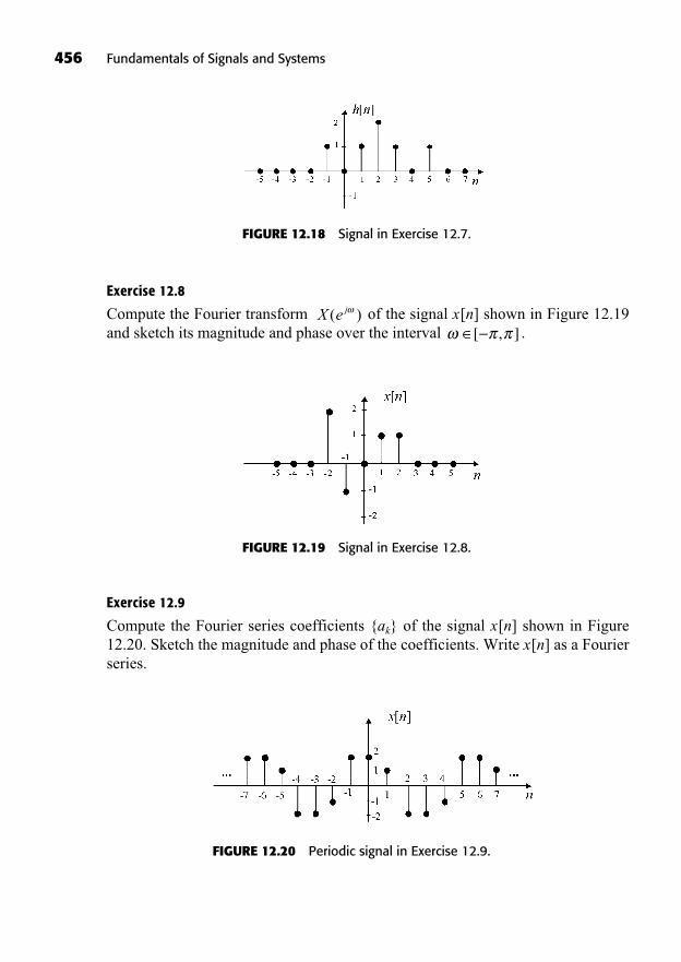
456 Fundamentals of Signals and Systems
Exercise 12.8
Compute the Fourier transform of the signal x[n] shown in Figure 12.19and sketch its magnitude and phase over the interval .[ , ]
X e j( )
FIGURE 12.18 Signal in Exercise 12.7.
FIGURE 12.19 Signal in Exercise 12.8.
Exercise 12.9
Compute the Fourier series coefficients {ak} of the signal x[n] shown in Figure12.20. Sketch the magnitude and phase of the coefficients. Write x[n] as a Fourierseries.
FIGURE 12.20 Periodic signal in Exercise 12.9.

Answer:
Exercise 12.10
Consider a DLTI system with impulse response .Compute the output signal y[n] for the input . Use the DTFT.
Exercise 12.11
Compute the Fourier transform of the signal
Answer:
.<1x n ne u n
j n n[ ] [ ],= 8 3 3X e j( )
x n u nn[ ] ( . ) [ ]= 0 2h n u n u nn n[ ] ( . ) [ ] ( . ) [ ]= 0 4 0 5 22
Discrete-Time Fourier Series and Fourier Transform 457

This page intentionally left blank
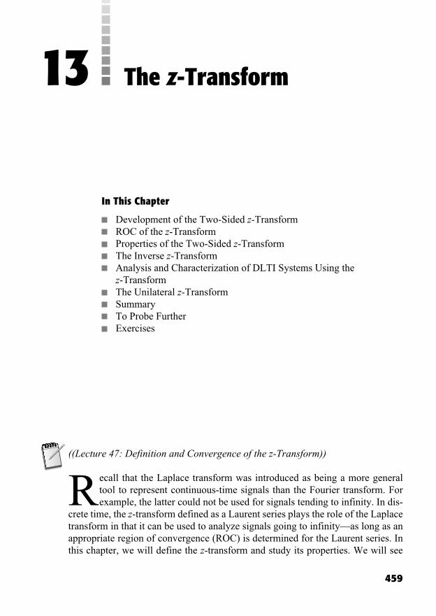
459
The z-Transform13
In This Chapter
Development of the Two-Sided z-TransformROC of the z-TransformProperties of the Two-Sided z-TransformThe Inverse z-TransformAnalysis and Characterization of DLTI Systems Using thez-TransformThe Unilateral z-TransformSummaryTo Probe FurtherExercises
((Lecture 47: Definition and Convergence of the z-Transform))
Recall that the Laplace transform was introduced as being a more generaltool to represent continuous-time signals than the Fourier transform. Forexample, the latter could not be used for signals tending to infinity. In dis-
crete time, the z-transform defined as a Laurent series plays the role of the Laplacetransform in that it can be used to analyze signals going to infinity—as long as anappropriate region of convergence (ROC) is determined for the Laurent series. Inthis chapter, we will define the z-transform and study its properties. We will see
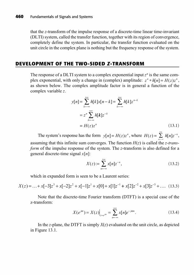
460 Fundamentals of Signals and Systems
that the z-transform of the impulse response of a discrete-time linear time-invariant(DLTI) system, called the transfer function, together with its region of convergence,completely define the system. In particular, the transfer function evaluated on theunit circle in the complex plane is nothing but the frequency response of the system.
DEVELOPMENT OF THE TWO-SIDED Z-TRANSFORM
The response of a DLTI system to a complex exponential input zn is the same com-plex exponential, with only a change in (complex) amplitude: ,as shown below. The complex amplitude factor is in general a function of thecomplex variable z.
(13.1)
The system’s response has the form , where ,
assuming that this infinite sum converges. The function H(z) is called the z-trans-form of the impulse response of the system. The z-transform is also defined for ageneral discrete-time signal x[n]:
(13.2)
which in expanded form is seen to be a Laurent series:
(13.3)
Note that the discrete-time Fourier transform (DTFT) is a special case of the z-transform:
(13.4)
In the z-plane, the DTFT is simply X(z) evaluated on the unit circle, as depictedin Figure 13.1.
X e X z x n ej
z e
j n
nj( ) ( ) [ ] .= =
==
+
X z x z x z x z x x z( ) [ ] [ ] [ ] [ ] [ ]= + + + + +… 3 2 1 0 13 2 1 1 ++ + +x z x z[ ] [ ] .2 32 3 …
X z x n z n
n
( ) : [ ] ,==
+
h n z n[ ]n=
+
H z( ) =y n H z zn[ ] ( )=
y n h k x n k h k z
z h
k
n k
k
n
[ ] [ ] [ ] [ ]
[
= =
=
=
+
=
+
kk z
H z z
k
k
n
]
( )=
+
=
z h n H z zn n=[ ] ( )

Figure 13.1 was done with the MATLAB script zTFmagsurface.m, which is lo-cated on the companion CD-ROM in D:\Chapter13.
Analogously, the continuous-time Fourier transform is the Laplace transformevaluated on the j -axis. Thus, the j -axis of the s-plane in continuous time cor-responds to the unit circle of the z-plane in discrete time.
Writing , we can analyze the convergence of the infinite summation inEquation 13.2:
(13.5)
We see that the convergence of the z-transform is equivalent to the conver-gence of the DTFT of the signal for any given circle in the z-plane ofradius r. That is,
(13.6)X re x n rj n( ) [ ] .= { }F
x n r n[ ]
X re x k r ej k j k
k
( ) ( [ ] ) .==
+
z re j=
The z-Transform 461
FIGURE 13.1 Relationship between the magnitudes of a z-transform and itscorresponding Fourier transform.
462 Fundamentals of Signals and Systems
Thus, the convergence of the z-transform will be described in terms of disk-shaped or annular regions of the z-plane centered at . Note that the exponen-tial weight multiplying the signal is either a constant-magnitude ordecaying exponential ( ), or a growing exponential ( ).
Example 13.1: The z-transform of the basic exponential signal is computed as follows:
(13.7)
The ROC of this z-transform is the region in the complex plane where valuesof z guarantee that , or equivalently . Then
(13.8)
A special case is the unit step signal u[n] ( ), whose z-transform is
(13.9)
Example 13.2: Consider the signal
(13.10)
Its z-transform is computed as follows.
X z u n u nn n
( ) [ ] [ ]= +1
32
1
21
= +
=
+
=
+
z
z z
n
n
n
n
n
n1
32
1
20 =
=
+
=
+
= +
n
n
n
n
n
n n
n
z z z
1
0 0
1
34 2
x n u n u nn n
[ ] [ ] [ ].= +1
32
1
21
U zz
z
zz( ) , .= = >
1
1 11
1
a = 1
X z azaz
z
z az an
n
( ) ( ) , .= = = >=
+1
01
1
1
z a>az <1 1
X z a z azn n
n
n
n
( ) ( ) .= ==
+
=
+
0
1
0
x n a u n an[ ] [ ],= �
0 1< <rr 1r rn , 0
z = 0
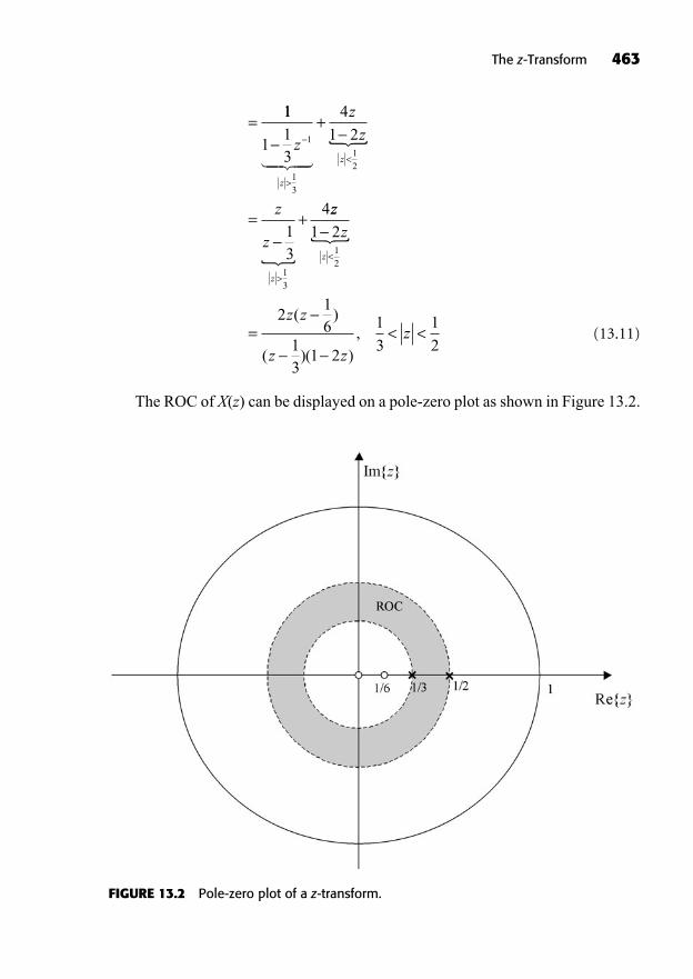
The z-Transform 463
(13.11)
The ROC of X(z) can be displayed on a pole-zero plot as shown in Figure 13.2.
=11
113
4
1 2
13
4
1
13
12
13
+
= +
>
<
>
z
z
z
z
z
z
z
z
��� ���
�
zz
z
z z
z zz
z
1 2
216
13
1 2
1
3
1
2
12
= < <
<
�
( )
( )( ),
FIGURE 13.2 Pole-zero plot of a z-transform.
464 Fundamentals of Signals and Systems
Note that a z-transform X(z) is rational whenever the signal x[n] is a linearcombination of real or complex exponentials.
ROC OF THE Z-TRANSFORM
Similar to the ROC of the Laplace transform, the ROC of the z-transform hasseveral properties that can help us find it. The ROC is the region of the z-plane( ) where the signal has a DTFT. That is, the ROC consists of values of z where the signal is absolutely summable; that is, .
Convergence is dependent only on r, not on . Hence, if X(z) exists at ,then it also converges on the circle . This guarantees that theROC will be composed of concentric rings. It can be shown that it is a single ring.This ring can extend inward to zero, in which case it becomes a disk, or extend out-ward to infinity. However, it is often bounded by poles, and the boundary of thering is open. We list some of the properties of ROCs of z-transforms.
The ROC of X(z) does not contain any poles.If x[n] is of finite duration, then the ROC is the entire z-plane, except possibly
and .
In this case, the finite sum of the z-transform converges for (almost) all z. Theonly two exceptions are because of the negative powers of z and be-
cause of the positive powers of z in .
If x[n] is right-sided, then the ROC of X (z) contains the exterior of a disk thateither extends to in the case , or does not include .If in addition, X(z) is rational, then the ROC is the open exterior of a diskbounded by the farthest pole from the origin.If x[n] is left-sided, then the ROC of X(z) contains the interior of a disk thateither includes in the case or does not include . If inaddition, X(z) is rational, then the ROC is the open disk bounded by the clos-est pole to the origin.If x[n] is two-sided, then the ROC of X(z) contains a ring with open boundariesin the z-plane. If in addition, X(z) is rational, then the ROC is an open ringbounded by poles of X(z).
Remarks:For a given pole-zero pattern, or equivalently, a rational X(z), there are a lim-ited number of ROCs that are consistent with the properties just described.The DTFT of a signal exists if the ROC of its z-transform includes the unit circle.
z = 0x n n[ ] ,= >0 0z = 0
z =x n n[ ] ,= <0 0z =
x n z n[ ]n n
n
= 1
2
X z( ) =z =z = 0
z =z = 0
z r e j=0
0 2,z r e j
0 00=
x k r k[ ] <k=
+
x n r n[ ]x n r n[ ]z re j=
((Lecture 48: Properties of the z-Transform))
PROPERTIES OF THE TWO-SIDED Z-TRANSFORM
The notation is used to represent a z-transform pair. In this section,we discuss the main properties of the z-transform. These properties are summarizedin Table D.11 in Appendix D.
Linearity
The operation of calculating the z-transform of a signal is linear.
For , ; if we form the linearcombination , then we have
(13.12)
Time Shifting
Time shifting leads to a multiplication by a complex exponential:
(13.13)
Scaling in the z-Domain
(13.14)
where the ROC is the scaled version of . Also, if X(z) has a pole or zero at, then has a pole or zero at . An important special case is
when . In this case , and
(13.15)
This corresponds to a counterclockwise rotation by an angle of radians ofthe pole-zero pattern of X(z). On the unit circle (i.e., the DTFT), this rotation cor-responds to a frequency shift.
0
e x n X e zj nZ
j0 0[ ] .( )z
0ROC ROC
X X=z e j
00=
z z a=0
X z z( )0
z a=ROC
X
z x n X znZ z
z0 00
[ ] ,, =ROC ROCX
x n n z X zZ n[ ] ( ), ,=
00 ROC ROC except possible
Xaaddition/removal of 0 or .
z n aX z bY zZ
[ ] ( ) ( ), .+ ROC ROC ROCX Y
z n ax n by n a b[ ] [ ] [ ], ,= + �y n Y z z
Z
[ ] ( ), ROCY
x n X z zZ
[ ] ( ), ROCX
x n X zZ
[ ] ( )
The z-Transform 465
Time Reversal
Reversing the time in signal x[n] leads to
(13.16)
that is, if , then .
Upsampling
The upsampled signal
(13.17)
has a z-transform given by:
(13.18)
That is, if , then . Also,
if X(z) has a pole (or a zero) at , then the z-transform of has
m poles (or m zeros) at . The upsampling prop-
erty can be interpreted through the power series representation of the z-transformin Equation 13.18:
(13.19)
Differentiation in the z-Domain
Differentiation of the z-transform with respect to z yields
(13.20)
Convolution of Two Signals
The convolution of x[n] and y[n] has a resulting z-transform given by
(13.21)x n y n x m y n m X z Y zm
Z
[ ] [ ] [ ] [ ] ( ) ( ),==
ROC ROCC ROCX Y
nx n zdX z
dz
Z
[ ]( )
, .=ROC ROCX
X z x n z x n zm mn
n
n
n m m m
( ) [ ] [ ], , , ,
= ==
+
=… 2 0 ,, ,
[ ] .2m
mn
n
x n z…
==
+
z r e k mm m jm
km
01
01
20
0 1/ / ( ), , ,= =
+…
x nm[ ]z r e j
0 00=
z r e k mm m jm
km
01
01
20
0 1/ / ( ), , ,= =
+ROC …z
0ROC
X
x n X zm
Zm m=[ ] ( ), ./ROC ROC
X1
x nx n m n m
m=[ ] :
[ ],
,
if is a multiple of
othe0 rrwise
z 1 ROCz ROCX
x n X zZ
[ ] ( ), ;=1 1ROC ROCX
466 Fundamentals of Signals and Systems

The z-Transform 467
Remark: The ROC can be larger than if pole-zero cancella-tions occur when forming the product .
First Difference
The first difference of a signal has the following z-transform:
(13.22)
Running Sum
The running sum, or accumulation, of a signal is the inverse of the first difference.
(13.23)
Conjugation
(13.24)
Remark: For x[n] real, we have: . Thus, if X(z) has a pole (or azero) at , it must also have a pole (or a zero) at . That is, all complexpoles and zeros come in conjugate pairs in the z-transform of a real signal.
Initial-Value Theorem
If x[n] is a signal that starts at n = 0, that is, , we have
(13.25)
This property follows from the power series representation of X(z):
(13.26)
Remark: For a transform X(z) expressed as a ratio of polynomials in z, the orderof its numerator cannot be greater than the order of its denominator for this prop-erty to apply, because then x[n] would have at least one nonzero value at negativetimes.
lim ( ) lim [ ] [ ] [ ]z z
X z x x z x z x= + + +( ) =0 1 21 2 … [[ ].0
x X zz
[ ] lim ( ).0 =
x n n[ ] ,= <0 0
z a=z a=X z X z( ) ( )=
x n X zZ
=[ ] ( ), .ROC ROCX
x mz
X z z zm
n Z
[ ]( )
( ), { : }=
>1
11
1ROC ROC
X�
x n x n z X z z zZ
[ ] [ ] ( ) ( ), : >{ }1 1 01 ROC ROCX
� ..
X z Y z( ) ( )ROC ROCX Y

Final-Value Theorem
If x[n] is a signal that starts at n = 0, that is, , we have
(13.27)
This formula gives us the residue at the pole z = 1 (which corresponds to DC).If this residue is nonzero, then X(z) has a nonzero final value.
((Lecture 49: The Inverse z-Transform))
THE INVERSE Z-TRANSFORM
The inverse z-transform is obtained by contour integration in the z-plane. This sec-tion presents a derivation of this result and discusses the use of the partial fractionexpansion technique to invert a z-transform.
Contour Integral
Consider the z-transform X(z) and let be in its ROC. Then, we can write
(13.28)
where denotes the operation of taking the Fourier transform. The inverseDTFT is then
(13.29)
and hence,
(13.30)
From , we getz re j=
x n r X re
rX re e d
n j
nj j n
[ ] ( )
( )
= { }=
=
F 1
22
1
2X re re dj j n( )( ) .
2
x n r X ren j[ ] ( ) ,= { }F 1
F {}
X re x n rj n( ) [ ] ,= { }F
z re j=
lim [ ] lim ( ).n z
x n z X z= ( )1
11
x n n[ ] ,= <0 0
468 Fundamentals of Signals and Systems

(13.31)
so that
(13.32)
where the integral is evaluated counterclockwise around the closed circular contourlying in the ROC (or any other circle centered at the origin in
the ROC) in the z-plane. Thus, the inverse z-transform formula is
(13.33)
From the theory of complex functions, we find that this integral is equal to thesum of the residues at the poles of contained in the closed contour (thisis the residue theorem). That is,
(13.34)
Example 13.3: Suppose that we want to compute the inverse z-transform of
. First, we form the product . Then, we take
the circle as the closed contour in the ROC. The function has onlyone pole at , and hence it has a single residue given by
(13.35)
Now, because the ROC of X(z) is the exterior of a disk (including infinity) ofradius equal to the magnitude of the outermost pole, the corresponding signal mustbe right-sided and causal. Therefore the inverse z-transform of X(z) is
(13.36)x n a u nn[ ] [ ].=
Resz a
n n
z a
nX z z z a X z z a= ={ } = =( ) ( ) ( ) .1 1
z a=z a= + >, 0
z
z a
n
X z zn( ) =1z a, >z
z a=X z( ) =
x n X z zn[ ] ( ) .= { }Residues 1
X z zn( ) 1
x nj
X z z dzn[ ] ( ) .=1
21
C�
C : := ={ }z z r�
x n X re re d
jX z z z dz
j j n
n
[ ] ( )( )
( )
=
=
1
2
1
2
2
1
CC
C
�
�=1
21
jX z z dzn( ) ,
dzdz
dd
d
dre d rje d
de
jrdz
z
j j
j
= = ( ) =
= =1dz
j
The z-Transform 469

Partial Fraction Expansion
An easier way to get the inverse z-transform is to expand X(z) in partial fractionsand use Table D.10 (Appendix D) of basic z-transform pairs. This technique isillustrated by two examples.
Example 13.4: Find the signal with z-transform
(13.37)
We first write X(z) as a rational function of z in order to find the poles and zeros:
(13.38)
It is clear that the poles are and the zeros are . Thepole-zero plot with the ROC is shown in Figure 13.3.
Noting that the transform in Equation 13.38 is a biproper rational function, thatis, the numerator and denominator are of the same order, we write the partial frac-tion expansion of X(z) as
(13.39)
where the ROCs of the individual terms are selected for consistency with the ROC. Coefficients A, B, and C are computed as follows.
(13.40)
(13.41)
(13.42)C z X zz
zzz
= =++
==
=
( ) ( )( ) (
11
1
105
13
113
2
12
113 22
4)=
B z X zz
zzz
= + =+
==
=
( ) ( )( ) (
11
1
512
112
2
13
112
553
3)=
A X zz
= ==
( )0
6
1
2< <z
1
3
X zz
z zA
B
z
z
( )( )( )
=+
+= +
+
<
1
1 1 1
2
12
1 13
1 12
1
12
���� �� ��� ��+
>
C
z
z
1 13
1
13
,
z j z j1 2= =,1
3p2 =,1
2p1 =
X zz
z zz( )
( )( ), .=
++
< <2
12
13
1 1
3
1
2
X zz z
z zz( )
( )( ), .=
++
< <1
12
1 131
1
3
1
2
470 Fundamentals of Signals and Systems
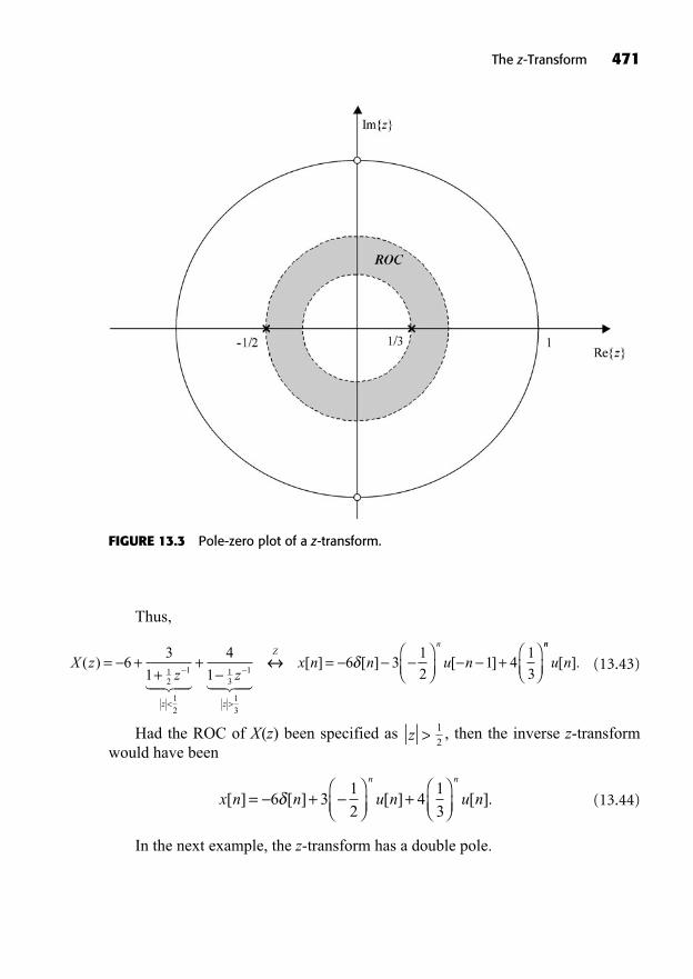
Thus,
(13.43)
Had the ROC of X(z) been specified as , then the inverse z-transformwould have been
(13.44)
In the next example, the z-transform has a double pole.
x n n u n u nn n
[ ] [ ] [ ] [ ].= + +6 31
24
1
3
>1
2z >
X zz z
z z
( ) = ++
+
< >
63
1
4
112
1
12
13
1
13
��� �� ��� ��= +
Zn
x n n u n[ ] [ ] [ ]6 31
21 4
1
3
nn
u n[ ].
The z-Transform 471
FIGURE 13.3 Pole-zero plot of a z-transform.
Example 13.5: Find the signal with z-transform:
(13.45)
We write X(z) as a rational function of z in order to find the poles and zeros:
(13.46)
The poles are (multiplicity m = 2), and the zeros are. The partial fraction expansion of X(z) can be expressed as follows,
where partial fractions of order 1 to m = 2 are included for the multiple pole:
(13.47)
where the ROCs of the individual terms are selected for consistency with the ROC. Coefficients A, B, and C are computed as follows.
(13.48)
(13.49)
(13.50)
Finally, the signal is obtained using Table D.10:
(13.51)
X zz z
z z
( )( )
=+
++
> >
78
25
1
1
6
5
1
112
1
12
12
1 2
��� ��112
13
1
13
48
25
1
1
78
25
� �� �� ��� ��+
=
>
z
x n
z
Z
[ ]11
2
6
51
1
2
48
25
1
3+ + +
n n
u n n u n[ ] ( ) [ ]n
u n[ ].
A X zB
z
C
z
B
zz z
=+
=
( )( ) ( )1 1
0
12
1 2 13
1
CC = =30
25
48
25
78
25
B z X zz z
zzz
= + =+
==
( ) ( )( )
11
12
1 212
1 2
13
112
==+
=2 453
6
5( )
C z X zz z
zzz
= =+
+=
==
( ) ( )( )
11
313
113
1 2
12
1 213
++=
952
48
252( )
>1
2z >
X zz z
z z
A
z
z
( )( ) ( )
=+
+=
+
>
1 2
12
1 2 13
1 12
1
1
1 1 1
22
12
1 2
12
13
1
13
1 1��� �� � �� �� ��
++
+
> >
B
z
C
z
z z
( )�� ��
,
z z1 2
0 1= =,
1
3p2 =
1
2p1 =
X zz z
z zz( )
( )
( ) ( ), .=
++
>1 1
212
2 13
X zz z
z zz( )
( ) ( ), .=
++
>1 2
12
1 2 13
11 1
1
2
472 Fundamentals of Signals and Systems
The z-Transform 473
Power Series Expansion
The definition of the z-transform is a power series whose coefficients equal the sig-nal values. Thus, given X(z), we can expand it in a power series and directly iden-tify the signal values to obtain the inverse z-transform.
Example 13.6: Usually the power series of a z-transform is infinite, and we can uselong division to obtain the signal values. For example, consider ,
. Long division yields
(13.52)
Note that the resulting power series converges because the ROC implies. Here, we can see a pattern, that is,
(13.53)
so that
(13.54)
Now suppose that the ROC is specified as the disk for the same
z-transform. Then, , and we can expand = asa power series with positive powers of z by long division:
(13.55)
+1 2 2
2 2
2
2 2
2
2 2 2
2 2
2 2
2 2 3 3
3 3
2 2 3
z z
z z
z
z z
z
z z
�
)zz3…
.
z
z
( . )
( . )+0 5
1 0 5
1
1z.
=1
1 0 5 1X z( ) =( . )0 5 11 <z
z < 0 5.
x n u nn[ ] ( . ) [ ].= 0 5
x n n n n k[ ] [ ] . [ ] ( . ) [ ] ( . )= + + + +1 0 5 1 0 5 2 0 52 … [[ ] ,n k +…
0 5 11. z <
1 0 5 1
1 0 5
0 5
0 5 0 5
0 5
1
1
1
1 2 2
.
.
.
. ( . )
( .
z
z
z
z z
)
))
. ( . )
.
2 2
1 2 21 0 5 0 5
z
z z+ + +
�
…
z .> 0 5z.
1
1 0 5 1X z( ) =
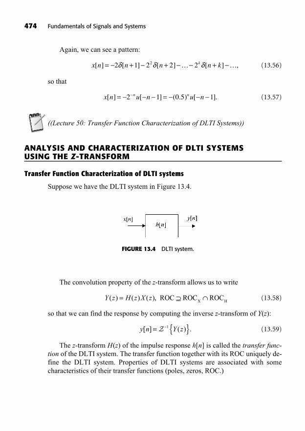
474 Fundamentals of Signals and Systems
Again, we can see a pattern:
(13.56)
so that
(13.57)
((Lecture 50: Transfer Function Characterization of DLTI Systems))
ANALYSIS AND CHARACTERIZATION OF DLTI SYSTEMS USING THE Z-TRANSFORM
Transfer Function Characterization of DLTI systems
Suppose we have the DLTI system in Figure 13.4.
x n u n u nn n[ ] [ ] ( . ) [ ].= =2 1 0 5 1
x n n n n kk[ ] [ ] [ ] [ ] ,= + + +2 1 2 2 22 … …
FIGURE 13.4 DLTI system.
The convolution property of the z-transform allows us to write
(13.58)
so that we can find the response by computing the inverse z-transform of Y(z):
(13.59)
The z-transform H(z) of the impulse response h[n] is called the transfer func-tion of the DLTI system. The transfer function together with its ROC uniquely de-fine the DLTI system. Properties of DLTI systems are associated with somecharacteristics of their transfer functions (poles, zeros, ROC.)
y n Y z[ ] ( ) .= { }Z-1
Y z H z X z( ) ( ) ( ),= ROC ROC ROCX H
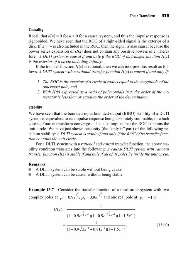
Causality
Recall that h[n] = 0 for n < 0 for a causal system, and thus the impulse response isright-sided. We have seen that the ROC of a right-sided signal is the exterior of adisk. If is also included in the ROC, then the signal is also causal because thepower series expansion of H(z) does not contain any positive powers of z. There-fore, A DLTI system is causal if and only if the ROC of its transfer function H(z)is the exterior of a circle including infinity.
If the transfer function H(z) is rational, then we can interpret this result as fol-lows. A DLTI system with a rational transfer function H(z) is causal if and only if:
1. The ROC is the exterior of a circle of radius equal to the magnitude of theoutermost pole, and
2. With H(z) expressed as a ratio of polynomials in z, the order of the nu-merator is less than or equal to the order of the denominator.
Stability
We have seen that the bounded-input bounded-output (BIBO) stability of a DLTIsystem is equivalent to its impulse response being absolutely summable, in whichcase its Fourier transform converges. This also implies that the ROC contains theunit circle. We have just shown necessity (the “only if” part) of the following re-sult on stability: A DLTI system is stable if and only if the ROC of its transfer func-tion contains the unit circle.
For a DLTI system with a rational and causal transfer function, the above sta-bility condition translates into the following: A causal DLTI system with rationaltransfer function H(z) is stable if and only if all of its poles lie inside the unit circle.
Remarks:A DLTI system can be stable without being causal.A DLTI system can be causal without being stable.
Example 13.7 Consider the transfer function of a third-order system with two
complex poles at and one real pole at :
(13.60)
H z
e z e z zj j
( )
( . )( . )( .
=+
1
1 0 9 1 0 9 1 1 54 1 4 1 11
1 2 1
1
1 0 9 2 0 81 1 1 5
)
( . . )( . ).=
+ +z z z
p3 1 5= .p e p ej j
14
240 9 0 9= =. , .
z =
The z-Transform 475
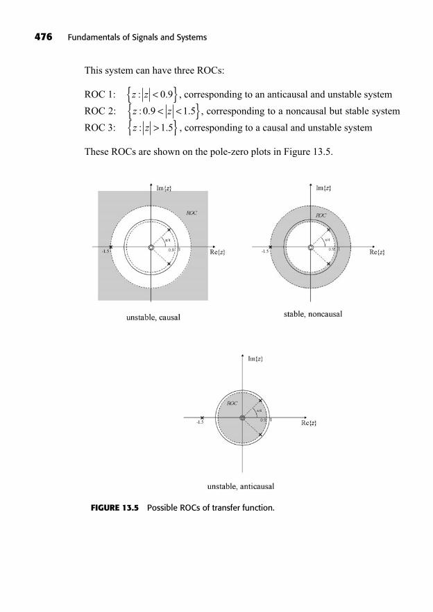
476 Fundamentals of Signals and Systems
This system can have three ROCs:
ROC 1: , corresponding to an anticausal and unstable system
ROC 2: , corresponding to a noncausal but stable system
ROC 3: , corresponding to a causal and unstable system
These ROCs are shown on the pole-zero plots in Figure 13.5.
z z: .>{ }1 5
z z: . .0 9 1 5< <{ }z z: .<{ }0 9
FIGURE 13.5 Possible ROCs of transfer function.
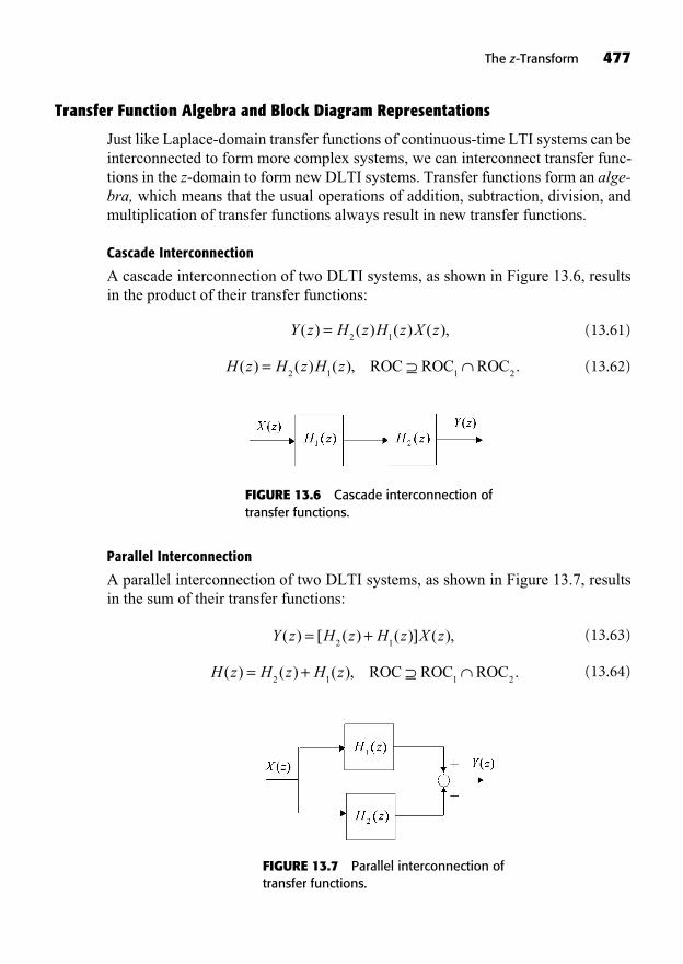
Transfer Function Algebra and Block Diagram Representations
Just like Laplace-domain transfer functions of continuous-time LTI systems can beinterconnected to form more complex systems, we can interconnect transfer func-tions in the z-domain to form new DLTI systems. Transfer functions form an alge-bra, which means that the usual operations of addition, subtraction, division, andmultiplication of transfer functions always result in new transfer functions.
Cascade Interconnection
A cascade interconnection of two DLTI systems, as shown in Figure 13.6, resultsin the product of their transfer functions:
(13.61)
(13.62)H z H z H z( ) ( ) ( ), .=2 1
ROC ROC ROC1 2
Y z H z H z X z( ) ( ) ( ) ( ),=2 1
The z-Transform 477
FIGURE 13.6 Cascade interconnection oftransfer functions.
Parallel Interconnection
A parallel interconnection of two DLTI systems, as shown in Figure 13.7, resultsin the sum of their transfer functions:
(13.63)
(13.64)H z H z H z( ) ( ) ( ), .= +2 1
ROC ROC ROC1 2
Y z H z H z X z( ) [ ( ) ( )] ( ),= +2 1
FIGURE 13.7 Parallel interconnection oftransfer functions.
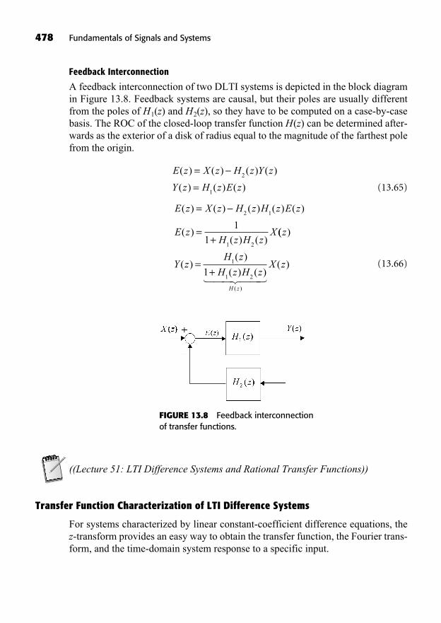
Feedback Interconnection
A feedback interconnection of two DLTI systems is depicted in the block diagramin Figure 13.8. Feedback systems are causal, but their poles are usually differentfrom the poles of H1(z) and H2(z), so they have to be computed on a case-by-casebasis. The ROC of the closed-loop transfer function H(z) can be determined after-wards as the exterior of a disk of radius equal to the magnitude of the farthest polefrom the origin.
(13.65)
(13.66)
E z X z H z H z E z
E zH z H z
X
( ) ( ) ( ) ( ) ( )
( )( ) ( )
=
=+
2 1
1 2
1
1(( )
( )( )
( ) ( )( )
( )
z
Y zH z
H z H zX z
H z
=+
1
1 21� ��� ���
E z X z H z Y z
Y z H z E z
( ) ( ) ( ) ( )
( ) ( ) ( )
==
2
1
478 Fundamentals of Signals and Systems
FIGURE 13.8 Feedback interconnectionof transfer functions.
((Lecture 51: LTI Difference Systems and Rational Transfer Functions))
Transfer Function Characterization of LTI Difference Systems
For systems characterized by linear constant-coefficient difference equations, thez-transform provides an easy way to obtain the transfer function, the Fourier trans-form, and the time-domain system response to a specific input.
Consider the Nth-order difference equation:
(13.67)
which can be expanded into
(13.68)
Using the time-shifting property of the z-transform, we directly obtain the z-transform on both sides of this equation:
(13.69)
or
(13.70)
The transfer function is then given by the z-transform of the output divided bythe z-transform of the input:
(13.71)
Hence, the transfer function of an LTI difference system is always rational. Ifthe difference equation is causal, which is the case in real-time signal processing,then the region of convergence of the transfer function will be the open exterior ofa disk of radius equal to the magnitude of the farthest pole from the origin. The re-gion of convergence of a transfer function obtained by taking the ratio of trans-forms of specific input and output signals must be consistent with the ROCs of Y(z)and X(z). Specifically, it must satisfy . If the rationaltransfer function is given without an ROC, then knowledge of system propertiessuch as causality or stability can help us find it.
Example 13.8: Consider a DLTI system defined by the difference equation
(13.72)
Taking the z-transform, we get
(13.73)Y z z Y z z X z( ) ( ) ( ),+ =1
321 1
y n y n x n[ ] [ ] [ ].+ =1
31 2 1
ROC ROC ROCY X H
H zY z
X z
b b z b z
a a z aM
M
N
( )( )
( )= =
+ + ++ + +
0 11
0 11
zz N.
( ) ( ) ( ) (a a z a z Y z b b z b z XN
NM
M0 1
10 1
1+ + + = + + + zz).
a z Y z b z X zk
k
k
N
kk
k
M
= =
=( ) ( )0 0
a y n a y n a y n N b x n b x nN0 1 0 1
1 1[ ] [ ] [ ] [ ] [ ]+ + + = + + + b x n MM
[ ].
a y n k b x n kk
k
N
kk
M
[ ] [ ],== =0 0
The z-Transform 479
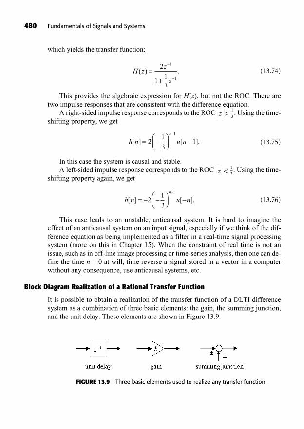
which yields the transfer function:
(13.74)
This provides the algebraic expression for H(z), but not the ROC. There aretwo impulse responses that are consistent with the difference equation.
A right-sided impulse response corresponds to the ROC . Using the time-shifting property, we get
(13.75)
In this case the system is causal and stable.A left-sided impulse response corresponds to the ROC . Using the time-
shifting property again, we get
(13.76)
This case leads to an unstable, anticausal system. It is hard to imagine theeffect of an anticausal system on an input signal, especially if we think of the dif-ference equation as being implemented as a filter in a real-time signal processingsystem (more on this in Chapter 15). When the constraint of real time is not anissue, such as in off-line image processing or time-series analysis, then one can de-fine the time n = 0 at will, time reverse a signal stored in a vector in a computerwithout any consequence, use anticausal systems, etc.
Block Diagram Realization of a Rational Transfer Function
It is possible to obtain a realization of the transfer function of a DLTI differencesystem as a combination of three basic elements: the gain, the summing junction,and the unit delay. These elements are shown in Figure 13.9.
h n u nn
[ ] [ ].= 21
3
1
1
3z <
h n u nn
[ ] [ ].= 21
31
1
1
3z >
H zz
z( ) .=
+
2
113
1
1
480 Fundamentals of Signals and Systems
FIGURE 13.9 Three basic elements used to realize any transfer function.
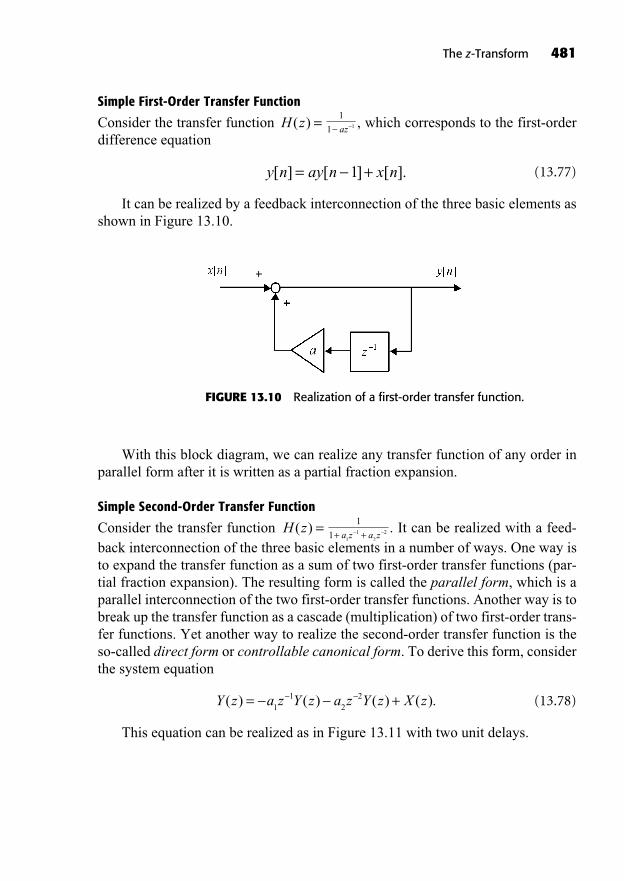
The z-Transform 481
Simple First-Order Transfer Function
Consider the transfer function , which corresponds to the first-orderdifference equation
(13.77)
It can be realized by a feedback interconnection of the three basic elements asshown in Figure 13.10.
y n ay n x n[ ] [ ] [ ].= +1
az
1
1 1H z( ) =
FIGURE 13.10 Realization of a first-order transfer function.
With this block diagram, we can realize any transfer function of any order inparallel form after it is written as a partial fraction expansion.
Simple Second-Order Transfer Function
Consider the transfer function . It can be realized with a feed-back interconnection of the three basic elements in a number of ways. One way isto expand the transfer function as a sum of two first-order transfer functions (par-tial fraction expansion). The resulting form is called the parallel form, which is aparallel interconnection of the two first-order transfer functions. Another way is tobreak up the transfer function as a cascade (multiplication) of two first-order trans-fer functions. Yet another way to realize the second-order transfer function is theso-called direct form or controllable canonical form. To derive this form, considerthe system equation
(13.78)
This equation can be realized as in Figure 13.11 with two unit delays.
Y z a z Y z a z Y z X z( ) ( ) ( ) ( ).= +1
12
2
a z a z+ +1
11
12
2H z( ) =

482 Fundamentals of Signals and Systems
Direct Form (Controllable Canonical Form)
A direct form can be obtained by breaking up the general transfer function in Equa-tion 13.79 into two subsystems as shown in Figure 13.12.
(13.79)
Assume without loss of generality that a0 = 1 (if not, just divide all bi’s by a0.)
H zY z
X z
b b z b z
a a z aM
M
N
( )( )
( )= =
+ + ++ + +
0 11
0 11
zz N
FIGURE 13.11 Realization of a second-ordertransfer function.
FIGURE 13.12 Transfer function as a cascade of two DLTI subsystems.
The input-output system equation of the first subsystem is
(13.80)
and for the second subsystem, we have
(13.81)
The direct form realization is then as shown in Figure 13.13 for a second-ordersystem.
Y z b W z b z W z b z W z b zM
MM
M( ) ( ) ( ) ( )= + + + ++0 1
11
1 WW z( ).
W z a z W z a z W z a z W z XN
NN
N( ) ( ) ( ) ( )= ++1
11
1 (( ),z
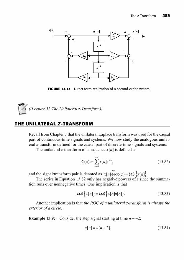
((Lecture 52:The Unilateral z-Transform))
THE UNILATERAL Z-TRANSFORM
Recall from Chapter 7 that the unilateral Laplace transform was used for the causalpart of continuous-time signals and systems. We now study the analogous unilat-eral z-transform defined for the causal part of discrete-time signals and systems.
The unilateral z-transform of a sequence x[n] is defined as
(13.82)
and the signal/transform pair is denoted as .The series in Equation 13.82 only has negative powers of z since the summa-
tion runs over nonnegative times. One implication is that
(13.83)
Another implication is that the ROC of a unilateral z-transform is always theexterior of a circle.
Example 13.9: Consider the step signal starting at time n = –2:
(13.84)x n u n[ ] [ ].= + 2
UZ UZx n x n u n[ ] [ ] [ ] .{ } = { }
x n z x nUZ
[ ] ( ) [ ]= { }X UZ
X ( ) : [ ] ,z x n z n
n
==
+
0
The z-Transform 483
FIGURE 13.13 Direct form realization of a second-order system.
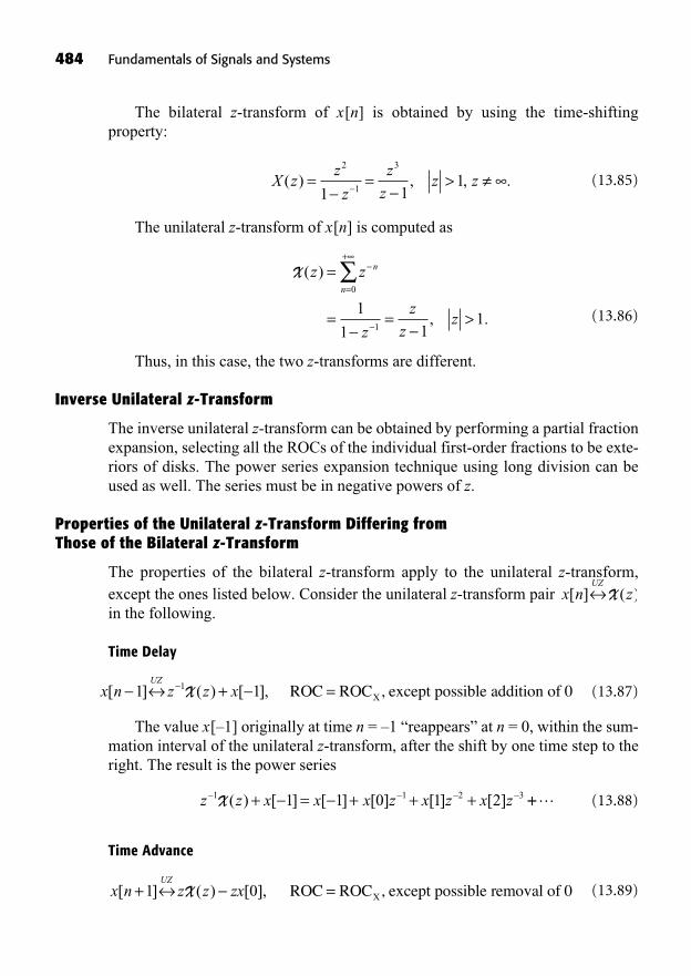
The bilateral z-transform of x[n] is obtained by using the time-shiftingproperty:
(13.85)
The unilateral z-transform of x[n] is computed as
(13.86)
Thus, in this case, the two z-transforms are different.
Inverse Unilateral z-Transform
The inverse unilateral z-transform can be obtained by performing a partial fractionexpansion, selecting all the ROCs of the individual first-order fractions to be exte-riors of disks. The power series expansion technique using long division can beused as well. The series must be in negative powers of z.
Properties of the Unilateral z-Transform Differing from Those of the Bilateral z-Transform
The properties of the bilateral z-transform apply to the unilateral z-transform, except the ones listed below. Consider the unilateral z-transform pair in the following.
Time Delay
(13.87)
The value x[–1] originally at time n = –1 “reappears” at n = 0, within the sum-mation interval of the unilateral z-transform, after the shift by one time step to theright. The result is the power series
(13.88)
Time Advance
(13.89)ROC ROC except possible removal of 0X= ,x n z z zxUZ
[ ] ( ) [ ],+1 0X
z z x x x z x z x z+ = + + +1 1 2 31 1 0 1 2X ( ) [ ] [ ] [ ] [ ] [ ] ++
ROC ROC except possible addition of 0X= ,x n z z xUZ
[ ] ( ) [ ],+1 11X
x n zUZ
[ ] ( )X
X ( )
, .
z z
z
z
zz
n
n
=
= = >
=
+
0
1
1
1 11
X zz
z
z
zz z( ) , , .= = >
2
1
3
1 11
484 Fundamentals of Signals and Systems
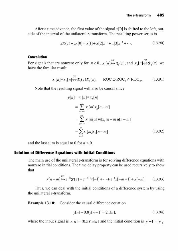
After a time advance, the first value of the signal x[0] is shifted to the left, out-side of the interval of the unilateral z-transform. The resulting power series is
(13.90)
Convolution
For signals that are nonzero only for , , and , wehave the familiar result
(13.91)
Note that the resulting signal will also be causal since
(13.92)
and the last sum is equal to 0 for n < 0.
Solution of Difference Equations with Initial Conditions
The main use of the unilateral z-transform is for solving difference equations withnonzero initial conditions. The time delay property can be used recursively to showthat
(13.93)
Thus, we can deal with the initial conditions of a difference system by usingthe unilateral z-transform.
Example 13.10: Consider the causal difference equation
(13.94)
where the input signal is and the initial condition is .y y[ ] =1 1x n u nn[ ] ( . ) [ ]= 0 5
y n y n x n[ ] . [ ] [ ],=0 8 1 2
x n m z z z x z x m xUZ
m m[ ] ( ) [ ] [ ] [+ + + + ++X 1 11 1 m].
y n x n x n
x m x n m
x m u
m
[ ] [ ] [ ]
[ ] [ ]
[ ]
=
=
=
=
+1 2
1 2
1[[ ] [ ] [ ]
[ ] [ ]
m x n m u n m
x m x n m
m
m
n
2
1 20
=
=
+
=
ROC ROC ROC1 2.x n x n z zUZ
1 2 1 2[ ] [ ] ( ) ( ),X X
x n zUZ
2 2[ ] ( )Xx n z
UZ
1 1[ ] ( )Xn 0
z z zx x x z x zX ( ) [ ] [ ] [ ] [ ] .= + + +0 1 2 31 2
The z-Transform 485
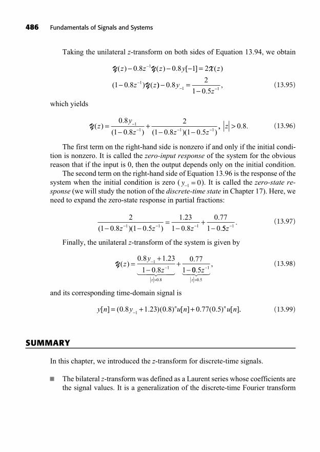
Taking the unilateral z-transform on both sides of Equation 13.94, we obtain
(13.95)
which yields
(13.96)
The first term on the right-hand side is nonzero if and only if the initial condi-tion is nonzero. It is called the zero-input response of the system for the obviousreason that if the input is 0, then the output depends only on the initial condition.
The second term on the right-hand side of Equation 13.96 is the response of thesystem when the initial condition is zero ( ). It is called the zero-state re-sponse (we will study the notion of the discrete-time state in Chapter 17). Here, weneed to expand the zero-state response in partial fractions:
(13.97)
Finally, the unilateral z-transform of the system is given by
(13.98)
and its corresponding time-domain signal is
(13.99)
SUMMARY
In this chapter, we introduced the z-transform for discrete-time signals.
The bilateral z-transform was defined as a Laurent series whose coefficients arethe signal values. It is a generalization of the discrete-time Fourier transform
y n y u n u nn n[ ] ( . . )( . ) [ ] . ( . ) [ ]= + +0 8 1 23 0 8 0 77 0 51
..
Y( ). .
.
.
.
zy
zz
=+
+
>
0 8 1 23
1 0 8
0 77
11
1
0 8
� ��� ��� 00 5 1
0 5
.,
.
zz >
� �� ��
2
1 0 8 1 0 5
1 23
1 0 8
0 77
1 01 1 1( . )( . )
.
.
.
.= +
z z z 55 1z.
y =1 0
Y( ).
( . ) ( . )( . )z
y
z z z= +
0 8
1 0 8
2
1 0 8 1 0 51
1 1 1,, . .z > 0 8
Y Y X
Y
( ) . ( ) . [ ] ( )
( . ) (
z z z y z
z z
=0 8 0 8 1 2
1 0 8
1
1 )) ..
,=0 82
1 0 51 1y
z
486 Fundamentals of Signals and Systems
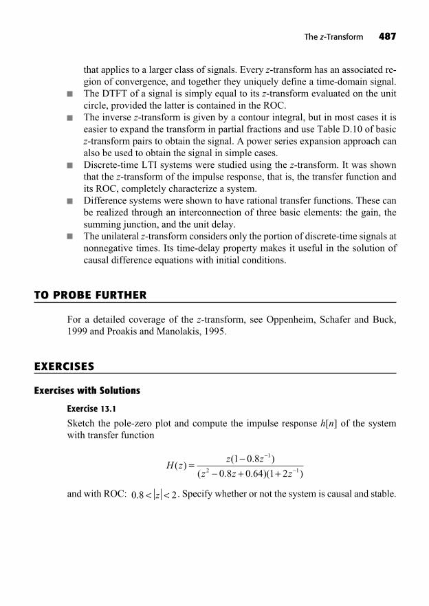
that applies to a larger class of signals. Every z-transform has an associated re-gion of convergence, and together they uniquely define a time-domain signal.The DTFT of a signal is simply equal to its z-transform evaluated on the unitcircle, provided the latter is contained in the ROC.The inverse z-transform is given by a contour integral, but in most cases it iseasier to expand the transform in partial fractions and use Table D.10 of basicz-transform pairs to obtain the signal. A power series expansion approach canalso be used to obtain the signal in simple cases.Discrete-time LTI systems were studied using the z-transform. It was shownthat the z-transform of the impulse response, that is, the transfer function andits ROC, completely characterize a system.Difference systems were shown to have rational transfer functions. These canbe realized through an interconnection of three basic elements: the gain, thesumming junction, and the unit delay.The unilateral z-transform considers only the portion of discrete-time signals atnonnegative times. Its time-delay property makes it useful in the solution ofcausal difference equations with initial conditions.
TO PROBE FURTHER
For a detailed coverage of the z-transform, see Oppenheim, Schafer and Buck,1999 and Proakis and Manolakis, 1995.
EXERCISES
Exercises with Solutions
Exercise 13.1
Sketch the pole-zero plot and compute the impulse response h[n] of the systemwith transfer function
and with ROC: . Specify whether or not the system is causal and stable.0 8 2. < <z
H zz z
z z z( )
( . )
( . . )( )=
+ +1 0 8
0 8 0 64 1 2
1
2 1
The z-Transform 487
Answer:
The coefficients are given by
Thus,
The inverse z-transform is obtained using Table D.10:
The pole-zero plot is shown in Figure 13.14.
h n j e u n jj
n
[ ] . . . [ ] .= +( ) +0 22 0 056 0 8 0 223 00 056 0 8 0 45 2 13. . [ ] . ( ) [( ) e u n u nj
n
n ]]
Re ( . . ) . [ ] .= + ( )2 0 22 0 056 0 8 03e j u nj n n
445 2 1
2 0 8 0 223
0 056
( ) [ ].
. . cos . sin= ( )
n
n
u n
n3
0 45 2 1n u n u nn[ ] . ( ) [ ]
H zj
e zj
z
( ). .
( . ).
=+
>
0 224 0 0555
1 0 8 3 1
0 8
� ��� ���� � ��� ���
+
>
0 224 0 0555
1 0 8 3 1
0 8
. .
( . ).
j
e zj
z
+<
0 449
1 2 1
2
.
( )zz
� �� ��
Cz z
e z e zj j
=1 1
3 1 3 1
1 0 8
1 0 8 1 0 8
( . )
( . )( . ))
.
( . . ).
z=
=+ +
=
2
0 7
1 0 4 0 160 449
Az z
e z zj
z
=+ =
1 1
3 1 10 8
1 0 8
1 0 8 1 2
( . )
( . )( ). ee
j j
j jj
e e
e e3
1 25 1
1 1 2 5
3 3
23
=+
. ( )
( )( . 3
3 3
23 3
1 25 1
3 5 2 5)
. ( )
( . .
=+
e e
e e
j j
j j))
. ( )
( . . )
=
=
1 2512
32
12
32
5 25 1 53
2
j j
j
== =+
= +
54
14
21 3 3
5 21 3 3
4680 224 0 0555
( )
( ). .
j
jj
H zz z
z z z
z z( )
( . )
( . . )( )
( .=
+ +=
0 8
0 8 0 64 2
1 0 82
1
+
1
3 1 3 1 11 0 8 1 0 8 1 2
0)
( . )( . )( )
,
e z e z zj j
..
( . )
*
( ..
8 2
1 0 8 1 03 1
0 8
< <
= +
>
z
A
e z
Aj
z
� ��� ��� 881 2
3 1
0 8
1
2e z
C
zj
zz
><
++
)( )
.
� ��� ���� �� ��
488 Fundamentals of Signals and Systems

The z-Transform 489
The system is not causal since the ROC is a ring, but it is stable, as it includesthe unit circle.
Exercise 13.2
Compute the inverse z-transform of using the powerseries expansion method.
Answer:
X zz
z
z
z( )
( . ),= =
1 0 5
2
2 11
2
z, .< 0 5z
z( . )1 0 5 1X z( ) =
FIGURE 13.14 Pole-zero plot of transfer function in Exercise 13.1.
Long division yields
Note that the resulting power series converges because the ROC implies. The signal is
Exercise 13.3
Consider the stable LTI system defined by its transfer function
(a) Sketch the pole-zero plot for this transfer function and give its ROC. Is thesystem causal?
Answer:The poles are . The zeros are . Thesystem is stable, so its ROC must include the unit circle. Because is finite,we can conclude that the system is causal. The pole-zero plot is shown in Figure13.15.
(b) Find the corresponding difference system relating the output y[n] to theinput x[n].
Answer:We first write the transfer function as a function of of the form
H zz z
z z( )
..=
++ +1 2
1 0 5
1 2
1 2
z 1
H ( )z z
1 22 1= =,p j p j1 20 5 0 5 0 5 0 5= + =. . , . .
H zz z
z z( )
..=
++ +
2
2
2
0 5
x n n n n
u nn
[ ] [ ] [ ] [ ]
( ) [
= + + +
= +
2 2 4 3 8 4
1
21
…
2].
2 1z <
+1 2 2
2 4
4
4 8
8
2 4 22
2 3
3
3 4
4
2 3 3 4
z z
z z
z
z z
z
z z z( )
)…
.
490 Fundamentals of Signals and Systems
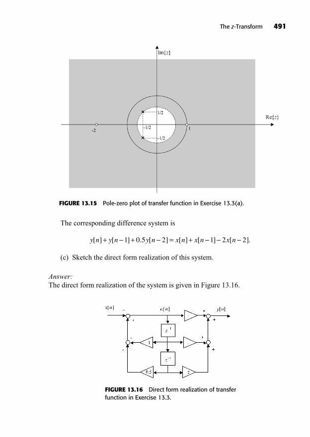
The z-Transform 491
The corresponding difference system is
(c) Sketch the direct form realization of this system.
Answer:The direct form realization of the system is given in Figure 13.16.
y n y n y n x n x n x n[ ] [ ] . [ ] [ ] [ ] [ ].+ + = +1 0 5 2 1 2 2
FIGURE 13.15 Pole-zero plot of transfer function in Exercise 13.3(a).
FIGURE 13.16 Direct form realization of transferfunction in Exercise 13.3.
Exercise 13.4 (a bit of actuarial mathematics using the unilateral z-transform…)
The balance of a bank account after each year with interest compounded annuallymay be described by the difference equation
where r is the annual interest rate, y[n] is the account balance at the beginning ofthe (n + 1)st year, the input “signal” is composed of Lconsecutive annual deposits of M dollars, and the initial condition is theinitial amount in the account before the first deposit.
(a) Is this system stable?
Answer:The system is unstable since the system is causal and the pole 1 + r is larger than1, that is, outside of the unit circle.
(b) Use the unilateral z-transform to compute Y(z).
Answer:Taking the unilateral z-transform on both sides, we obtain
(c) Find the annual deposit M as a function of the final balance in the accountafter L years, , and the interest rate r. Compute the annual depositM if you want to accrue $100,000 after 20 years at 5% annual interest ratewith an initial balance of .y =1 1000$
y L[ ]1
Y Y X
Y
( ) ( ) [ ] ( )
( )[
z r z z y z
zr y
+( ) +( ) ==
+( )1 1
1
1
11
1 1 1 1
1 1
1 1
] ( )
( )[ ]
+( ) ++( )
=+( )
r z
z
r z
zr y
X
Y11 1
1
1 1 1
1
1 1 1+( ) ++( )
=
r z
M z
r z z
L( )
( )
++( ) +
+( )r y z M z
r z
L[ ]( ) ( )
(
1 1 1
1 1 1
1
1 zz
r y M z k
k
L
==+( ) +
1
01 1
)
[ ]
more useful form:11
11 1+( )r z.
y y[ ] =1 1
x n M u n u n L[ ] ( [ ] [ ])=
y n r y n x n[ ] [ ] [ ],= +( ) +1 1
492 Fundamentals of Signals and Systems
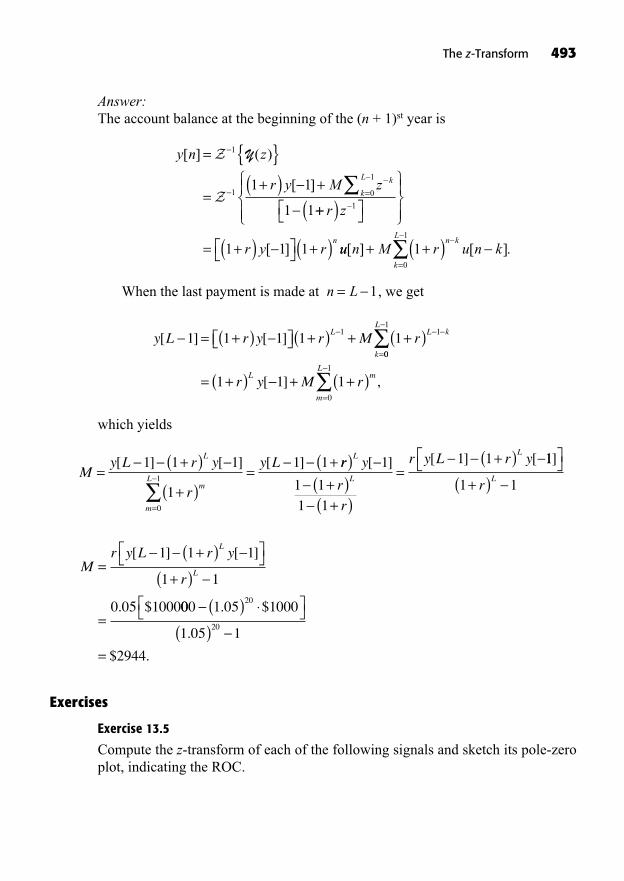
Answer:The account balance at the beginning of the (n + 1)st year is
When the last payment is made at , we get
which yields
Exercises
Exercise 13.5
Compute the z-transform of each of the following signals and sketch its pole-zeroplot, indicating the ROC.
Mr y L r y
r
L
L=+( )
+( )
=
[ ] [ ]
. $
1 1 1
1 1
0 05 1000000 1 05 1000
1 05 1
2944
20
20
( )( )
=
. $
.
$ .
My L r y
r
y LL
m
m
L=+( )+( )
=+
=
[ ] [ ] [ ]1 1 1
1
1 1
0
1
rr y
r
r
r y L r yL
L
L
( )+( )+( )
=+( )[ ] [ ] [1
1 1
1 1
1 1 11
1 1
]
+( )r L
y L r y r M rL L k
k
[ ] [ ]= +( ) +( ) + +( )=
1 1 1 1 11 1
00
1
0
1
1 1 1
L
L m
m
L
r y M r=
= +( ) + +( )[ ] ,
n L= 1
y n z
r y M z k
k
L
[ ] ( )
[ ]
= { }
=+( ) +
=
Z
Z
1
1 0
11 1
1 1
Y
++( )= +( ) +( )
r z
r y rn
1
1 1 1[ ] uu n M r u n kn k
k
L
[ ] [ ].+ +( )=
10
1
The z-Transform 493
494 Fundamentals of Signals and Systems
(a) Use the values ,for the pole-zero plot.
(b)
(c)
Answer:
Exercise 13.6
Compute the inverse z-transform of using the powerseries expansion method.
Exercise 13.7
Consider the following so-called auto-regressive moving-average causal filter Sinitially at rest:
S: (a) Compute the z-transform of the impulse response of the filter H(z) (the
transfer function) and give its ROC. Sketch the pole-zero plot.
(b) Compute the impulse response h[n] of the filter.
(c) Compute the frequency response of the filter. Plot its magnitude. Whattype of filter is it (lowpass, highpass, or bandpass)?
(d) Compute and sketch the step response s[n] of the filter.
Answer:
Exercise 13.8
Consider a DLTI system with transfer function .(a) Sketch the pole-zero plot of the system.
(b) Find the ROC that makes this system stable.
(c) Is the system causal with the ROC that you found in (b)? Justify youranswer.
(d) Suppose that is bounded for all frequencies. Find the response ofthe system y[n] to the input .x n u n[ ] [ ]=
H e j( )
z z
z z
.
( . )( . )+
3 41 2
0 8 0 8H z( ) =
y n y n y n x n x n[ ] . [ ] . [ ] [ ] [ ]+ =0 9 1 0 81 2 2
z, . < <0 2z
z .+
2
0 2X z( ) =
x n u nn[ ] ( ) [ ]= +2 3
x n u n u n[ ] [ ] [ ]= + 44
=
3
4= =1 5 0. ,x n n u nn[ ] cos( ) [ ], .= + >0 1
The z-Transform 495
Exercise 13.9
Compute the inverse z-transform x[n] of using themethod of long division and sketch it.
Answer:
Exercise 13.10
Sketch the pole-zero plot and compute the impulse response h[n] of the stable sys-tem with transfer function
Specify its ROC. Specify whether or not the system is causal.
Exercise 13.11
Consider the DLTI system with transfer function .(a) Sketch the pole-zero plot of the system.
(b) Find the ROC that makes this system stable.
(c) Is the system causal with the ROC that you found in (b)? Justify youranswer.
(d) Suppose that is bounded for all frequencies. Calculate the responseof the system y[n] to the input x[n] = u[n].
Answer:
H e j( )
z
z z( . )+1
0 41H z( ) =
H zz z z
z z( )
( )( ).=
+ ++
2000 1450 135
100 81 5 4
3 2
2
z, .> 0 4z z( . )+1
0 4X z( ) =

This page intentionally left blank
497
Time and FrequencyAnalysis of Discrete-TimeSignals and Systems
14
((Lecture 53: Relationship Between the DTFT and the z-Transform))
We have seen that the discrete-time Fourier transform (DTFT) of asystem’s impulse response (the frequency response of the system) existswhenever the system is bounded-input bounded-output stable or,
equivalently, whenever the region of convergence (ROC) of the system’s transferfunction includes the unit circle. Then, the frequency response of the system issimply its transfer function H(z) evaluated on the unit circle , that is, .In this chapter, we discuss the geometric relationship between the poles and zeros
z e j=z = 1
In This Chapter
Geometric Evaluation of the DTFT from the Pole-Zero PlotFrequency Analysis of First-Order and Second-Order SystemsIdeal Discrete-Time FiltersInfinite Impulse Response and Finite Impulse Response FiltersSummaryTo Probe FurtherExercises
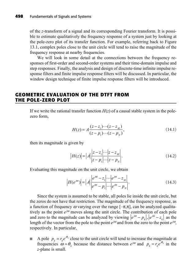
498 Fundamentals of Signals and Systems
of the z-transform of a signal and its corresponding Fourier transform. It is possi-ble to estimate qualitatively the frequency response of a system just by looking atthe pole-zero plot of its transfer function. For example, referring back to Figure13.1, complex poles close to the unit circle will tend to raise the magnitude of thefrequency response at nearby frequencies.
We will look in some detail at the connections between the frequency re-sponses of first-order and second-order systems and their time-domain impulse andstep responses. Finally, the analysis and design of discrete-time infinite impulse re-sponse filters and finite impulse response filters will be discussed. In particular, thewindow design technique of finite impulse response filters will be introduced.
GEOMETRIC EVALUATION OF THE DTFT FROM THE POLE-ZERO PLOT
If we write the rational transfer function H(z) of a causal stable system in the pole-zero form,
(14.1)
then its magnitude is given by
(14.2)
Evaluating this magnitude on the unit circle, we obtain
(14.3)
Since the system is assumed to be stable, all poles lie inside the unit circle, butthe zeros do not have that restriction. The magnitude of the frequency response, asa function of frequency varying over the range [– , ], can be analyzed qualita-tively as the point e j moves along the unit circle. The contribution of each poleand zero to the magnitude can be analyzed by viewing as thelength of the vector from the pole to the point e j and from the zero to the point e j ,respectively. In particular,
A pole close to the unit circle will tend to increase the magnitude atfrequencies because the distance between e j and in the z-plane is small.
p r ek k
j k=k
p r ek k
j k=
e p e zjk
jk
,
H e Ae z e z
e p e pj
j jM
j jN
( ) .= 1
1
H z Az z z z
z p z pM
N
( ) .= 1
1
H z Az z z z
z p z pM
N
( )( ) ( )
( ) ( ),= 1
1

A zero close to the unit circle will tend to decrease the magnitude atfrequencies .
The phase of is given by
(14.4)
Thus, the total phase is the sum of the individual angles of the pole and zerofactors seen as vectors in the z-plane and the phase of the gain A.
First-Order Systems
Consider the first-order causal system with :
(14.5)
This system is stable, and hence it has a Fourier transform given by
(14.6)
The geometric interpretation described above can be depicted on the pole-zeroplot shown in Figure 14.1, where a is real, 0 < a < 1.
H eae
e
e aj
j
j
j( ) .= =
1
1
H zaz
z
z az a( ) , .= = >
1
1 1
a <1
e p e zjk
jk
,
= + + + +H e A e z e z e zj j j jM
( ) ( ) ( ) ( )1 2
( ) ( ) ( ).e p e p e pj j jM1 2
H e j( )
k
z r ek k
j k=
Time and Frequency Analysis of Discrete-Time Signals and Systems 499
FIGURE 14.1 Pole-zero plot showing the vectorsassociated with the pole-zero form of a first-ordertransfer function with one real positive pole.
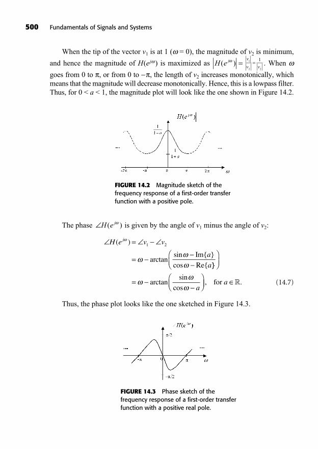
500 Fundamentals of Signals and Systems
When the tip of the vector v1 is at 1 ( = 0), the magnitude of v2 is minimum,
and hence the magnitude of H(ej ) is maximized as . When
goes from 0 to , or from 0 to , the length of v2 increases monotonically, whichmeans that the magnitude will decrease monotonically. Hence, this is a lowpass filter.Thus, for 0 < a < 1, the magnitude plot will look like the one shown in Figure 14.2.
v
v v=1
2 2
1H e j( ) =
FIGURE 14.2 Magnitude sketch of thefrequency response of a first-order transferfunction with a positive pole.
The phase is given by the angle of v1 minus the angle of v2:
(14.7)
Thus, the phase plot looks like the one sketched in Figure 14.3.
=
=
H e v v
a
a
j( )
arctansin Im{ }
cos Re{
1 2
}}
arctansin
cos, .=
aafor �
H e j( )
FIGURE 14.3 Phase sketch of thefrequency response of a first-order transferfunction with a positive real pole.
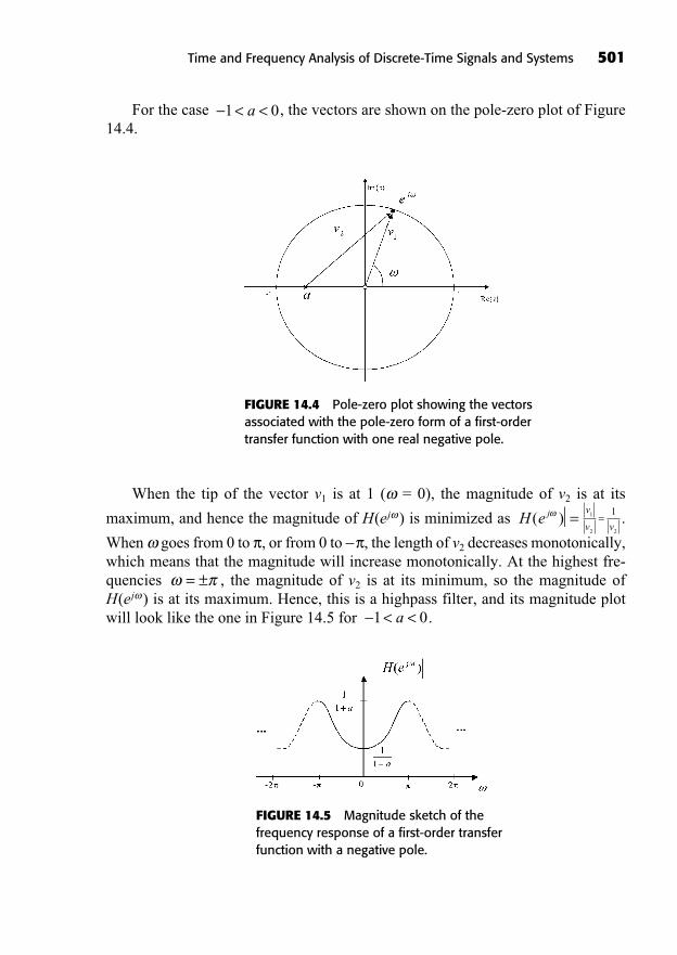
For the case , the vectors are shown on the pole-zero plot of Figure14.4.
< <1 0a
Time and Frequency Analysis of Discrete-Time Signals and Systems 501
FIGURE 14.4 Pole-zero plot showing the vectorsassociated with the pole-zero form of a first-ordertransfer function with one real negative pole.
When the tip of the vector v1 is at 1 ( = 0), the magnitude of v2 is at its
maximum, and hence the magnitude of H(ej ) is minimized as .
When goes from 0 to , or from 0 to , the length of v2 decreases monotonically,which means that the magnitude will increase monotonically. At the highest fre-quencies , the magnitude of v2 is at its minimum, so the magnitude ofH(ej ) is at its maximum. Hence, this is a highpass filter, and its magnitude plotwill look like the one in Figure 14.5 for .< <1 0a
= ±
v
v v=1
2 2
1H e j( ) =
FIGURE 14.5 Magnitude sketch of thefrequency response of a first-order transferfunction with a negative pole.

The phase is again given by the angle of v1 minus the angle of v2 asexpressed in Equation 14.7. It should look like the phase sketched in Figure 14.6.
H e j( )
502 Fundamentals of Signals and Systems
FIGURE 14.6 Phase sketch of thefrequency response of a first-order transferfunction with a negative real pole.
Second-Order Systems
Consider the stable second-order causal system with poles at :
(14.8)
The impulse response of this system is obtained from Table D.10 and by usingthe linearity and time-advance properties of the z-transform:
(14.9)
Its Fourier transform is given by
(14.10)
The magnitude of H(ej ) can be analyzed qualitatively by looking at the pole-zero plot in Figure 14.7 showing the vectors as defined above.
H ee
e r e re
e re
jj
j j
j
j j
( )cos
( )
=+
=
2
2 2
2
2
(( ).
e rej j
h n r n u nn[ ]sin
sin ( ) [ ].= +( )11
H zr z r z
z
z r z rz r( )
cos cos,=
+=
+>
1
1 2 21 2 2
2
2 2..
p re rj1 2
0 1,
,= < <±
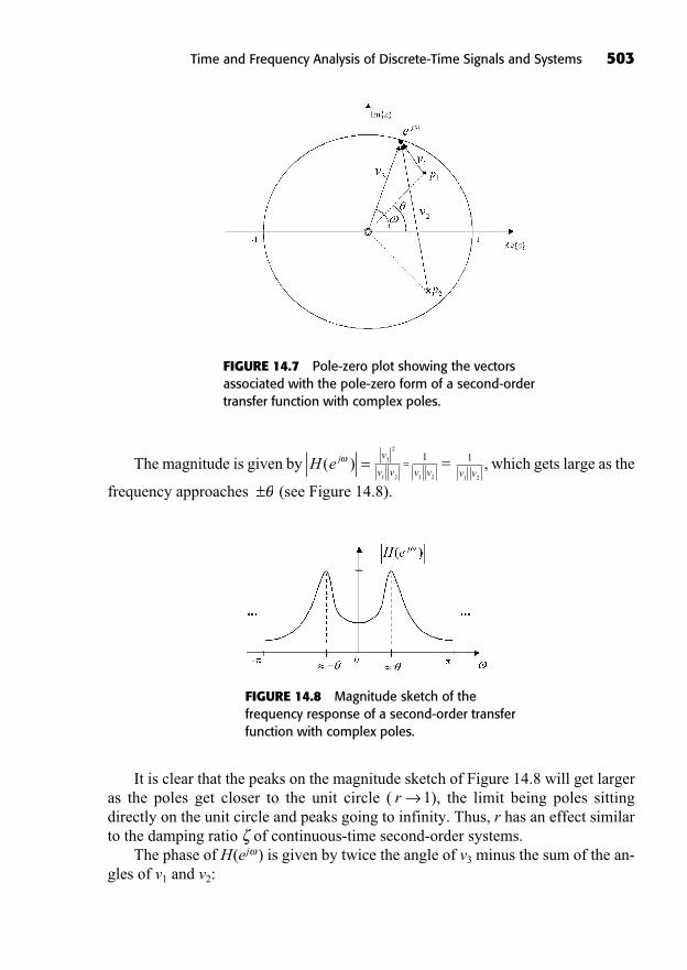
The magnitude is given by = , which gets large as the
frequency approaches (see Figure 14.8).±v v
1 2
1v
v v v v=3
2
1 2 1 2
1H e j( ) =
Time and Frequency Analysis of Discrete-Time Signals and Systems 503
FIGURE 14.7 Pole-zero plot showing the vectorsassociated with the pole-zero form of a second-ordertransfer function with complex poles.
FIGURE 14.8 Magnitude sketch of thefrequency response of a second-order transferfunction with complex poles.
It is clear that the peaks on the magnitude sketch of Figure 14.8 will get largeras the poles get closer to the unit circle ( ), the limit being poles sittingdirectly on the unit circle and peaks going to infinity. Thus, r has an effect similarto the damping ratio of continuous-time second-order systems.
The phase of H(ej ) is given by twice the angle of v3 minus the sum of the an-gles of v1 and v2:
r 1
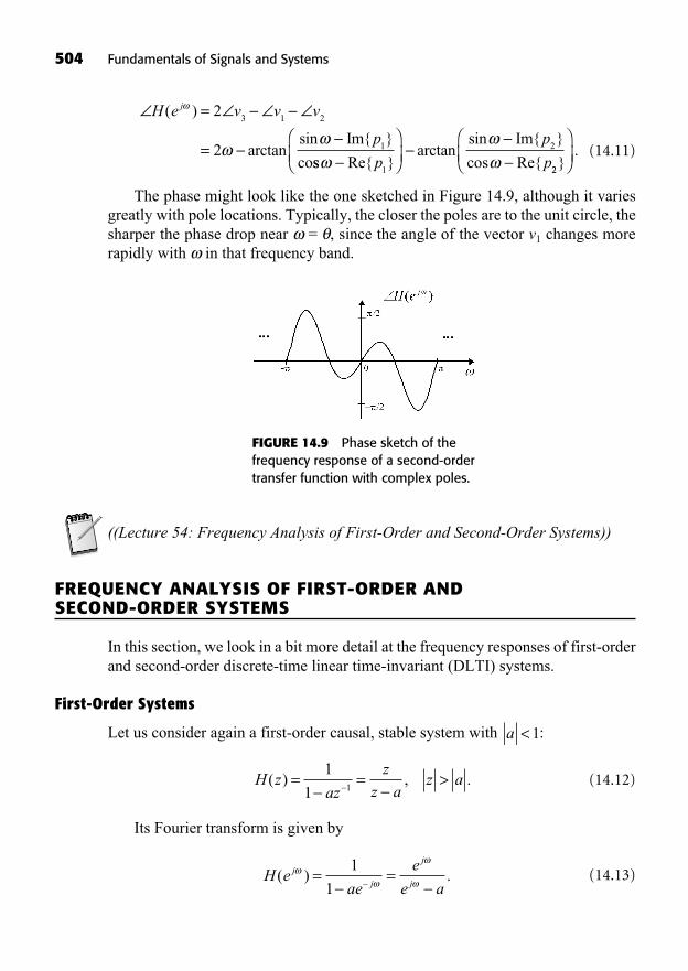
(14.11)
The phase might look like the one sketched in Figure 14.9, although it variesgreatly with pole locations. Typically, the closer the poles are to the unit circle, thesharper the phase drop near = , since the angle of the vector v1 changes morerapidly with in that frequency band.
=
=
H e v v v
p
j( )
arctansin Im{ }
co
2
2
3 1 2
1
ss Re{ }arctan
sin Im{ }
cos Re{p
p
p1
2
22}
.
504 Fundamentals of Signals and Systems
FIGURE 14.9 Phase sketch of thefrequency response of a second-ordertransfer function with complex poles.
((Lecture 54: Frequency Analysis of First-Order and Second-Order Systems))
FREQUENCY ANALYSIS OF FIRST-ORDER AND SECOND-ORDER SYSTEMS
In this section, we look in a bit more detail at the frequency responses of first-orderand second-order discrete-time linear time-invariant (DLTI) systems.
First-Order Systems
Let us consider again a first-order causal, stable system with :
(14.12)
Its Fourier transform is given by
(14.13)H eae
e
e aj
j
j
j( ) .= =
1
1
H zaz
z
z az a( ) , .= = >
1
1 1
a <1
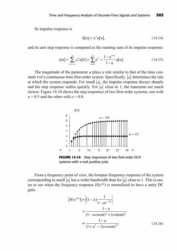
Its impulse response is
(14.14)
and its unit step response is computed as the running sum of its impulse response:
(14.15)
The magnitude of the parameter a plays a role similar to that of the time con-stant of a continuous-time first-order system. Specifically, determines the rateat which the system responds. For small , the impulse response decays sharplyand the step response settles quickly. For close to 1, the transients are muchslower. Figure 14.10 shows the step responses of two first-order systems, one witha = 0.5 and the other with a = 0.8.
aa
a
s n a u k aa
au nk
k
nk
k
n n
[ ] [ ] [ ].= = == =
+
0
11
1
h n a u nn[ ] [ ],=
Time and Frequency Analysis of Discrete-Time Signals and Systems 505
FIGURE 14.10 Step responses of two first-order DLTIsystems with a real positive pole.
From a frequency point of view, the lowpass frequency response of the systemcorresponding to small has a wider bandwidth than for close to 1. This is eas-ier to see when the frequency response H(ej ) is normalized to have a unity DCgain:
(14.16)
H e aae
a
a a
jj( )
( cos ) ( sin )
= ( )
=+
11
1
1
1 2 2
==+
1
1 22 1 2
a
a a( cos ) /
aa

506 Fundamentals of Signals and Systems
The magnitude in Equation 14.16 is plotted in Figure 14.11 for the cases a =0.5 and a = 0.8.
FIGURE 14.11 Magnitude of the frequency responses of first-ordertransfer functions with positive poles.
The phase changes more abruptly around DC for close to 1, as shown inFigure 14.12.
(14.17)=H ea
aj( ) arctansin
cos, .for �
a
FIGURE 14.12 Phase of the frequency responses of first-ordertransfer functions with positive poles.
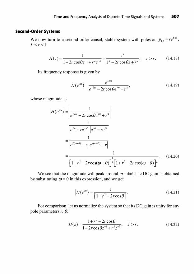
Second-Order Systems
We now turn to a second-order causal, stable system with poles at :
(14.18)
Its frequency response is given by
(14.19)
whose magnitude is
(14.20)
We see that the magnitude will peak around = ± . The DC gain is obtainedby substituting = 0 in this expression, and we get
(14.21)
For comparison, let us normalize the system so that its DC gain is unity for anypole parameters r, :
(14.22)H zr r
r z r zz r( )
cos
cos, .=
++
>1 2
1 2
2
1 2 2
H er r
j( )cos
.0
2
1
1 2=
+
H ee r e r
e re e re
j
j j
j j j j
( )cos
=+
=
1
2
1
2 2
=
=+ +
+
1
1
1 22
e r e r
r r
j j( ) ( )
cos( )112 2
121 2+ r r cos( )
.
H ee
e r e rj
j
j j( )
cos,=
+
2
2 22
H zr z r z
z
z r z rz r( )
cos cos,=
+=
+>
1
1 2 21 2 2
2
2 2..
r0 1< <p re j
1 2,,= ±
Time and Frequency Analysis of Discrete-Time Signals and Systems 507

Then,
(14.23)
Figure 14.13 shows the frequency response magnitude of the second-ordersystem for = and two values of pole magnitude, namely r = 0.6 and r = 0.8.4
H er r
r r r
j( )cos
cos( )=
+
+ + +
1 2
1 2 1
2
212 2 2
12r cos( )
.
508 Fundamentals of Signals and Systems
FIGURE 14.13 Frequency response magnitude of second-order transferfunctions with two pole magnitudes.
The phase of the frequency response for = in Equation 14.24 is shown inFigure 14.14 for r = 0.6 and r = 0.8.
(14.24)
The impulse response of this system for = is
(14.25)h n r n u nn[ ] sin ( ) [ ].= +2 14
4
=H er
rj( ) arctan
sin sin
cos cos2
+arctan
sin sin
cos cos.
r
r
4
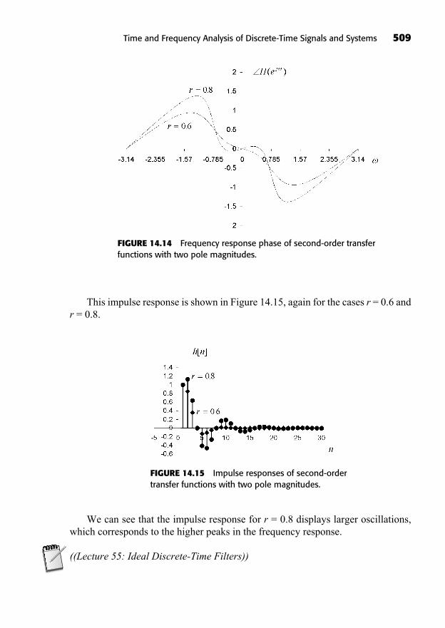
This impulse response is shown in Figure 14.15, again for the cases r = 0.6 andr = 0.8.
Time and Frequency Analysis of Discrete-Time Signals and Systems 509
FIGURE 14.14 Frequency response phase of second-order transferfunctions with two pole magnitudes.
FIGURE 14.15 Impulse responses of second-ordertransfer functions with two pole magnitudes.
We can see that the impulse response for r = 0.8 displays larger oscillations,which corresponds to the higher peaks in the frequency response.
((Lecture 55: Ideal Discrete-Time Filters))
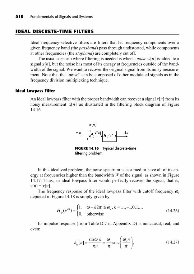
IDEAL DISCRETE-TIME FILTERS
Ideal frequency-selective filters are filters that let frequency components over agiven frequency band (the passband) pass through undistorted, while componentsat other frequencies (the stopband) are completely cut off.
The usual scenario where filtering is needed is when a noise w[n] is added to asignal x[n], but the noise has most of its energy at frequencies outside of the band-width of the signal. We want to recover the original signal from its noisy measure-ment. Note that the “noise” can be composed of other modulated signals as in thefrequency division multiplexing technique.
Ideal Lowpass Filter
An ideal lowpass filter with the proper bandwidth can recover a signal x[n] from itsnoisy measurement as illustrated in the filtering block diagram of Figure14.16.
x n[ ]
510 Fundamentals of Signals and Systems
FIGURE 14.16 Typical discrete-timefiltering problem.
In this idealized problem, the noise spectrum is assumed to have all of its en-ergy at frequencies higher than the bandwidth W of the signal, as shown in Figure14.17. Thus, an ideal lowpass filter would perfectly recover the signal, that is, y[n] = x[n].
The frequency response of the ideal lowpass filter with cutoff frequency c
depicted in Figure 14.18 is simply given by
(14.26)
Its impulse response (from Table D.7 in Appendix D) is noncausal, real, andeven:
(14.27)h nn
n
nlp
c c c[ ]sin
,= = sinc
H ek k
lpj c( )
, , , , , ,
,=
=1 2 1 0 1
0
… …otherwise
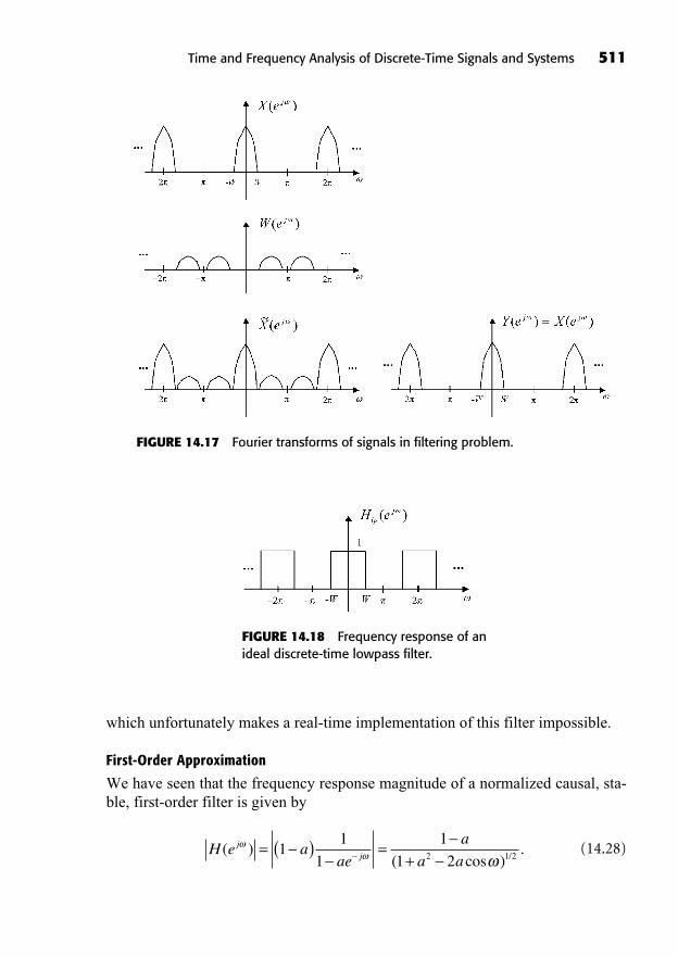
which unfortunately makes a real-time implementation of this filter impossible.
First-Order Approximation
We have seen that the frequency response magnitude of a normalized causal, sta-ble, first-order filter is given by
(14.28)H e aae
a
a aj
j( )( cos )
./= ( ) =+
11
1
1
1 22 1 2
Time and Frequency Analysis of Discrete-Time Signals and Systems 511
FIGURE 14.17 Fourier transforms of signals in filtering problem.
FIGURE 14.18 Frequency response of anideal discrete-time lowpass filter.

Suppose the cutoff frequency c (bandwidth) of the filter is defined as the fre-quency where the magnitude is 3 dB. Then, we can find an expression for the realpole in terms of the cutoff frequency c.
(14.29)
This quadratic equation can be solved for the pole
(14.30)
Note that the plus sign leads to a pole larger than one; hence we select
(14.31)
The poles corresponding to different cutoff frequencies as given by Equation14.31 are listed in Table 14.1.
a c=( . cos )
. .( . cos
2 1 0024
0 9976
1
0 99762 1 0024
c) . .2 0 9952
a c c= ±( . cos )
.
( . cos )2 1 0024
0 9976
1
2
2 1 0024
0
2
..( . cos )
. .( .
24884
2 1 0024
0 9976
1
0 99762 1= ±c 00024 0 99522cos ) .
c
=+
3 201
1 2
10
10 2 1 2
32
dB log( cos ) /
a
a a c
002 1 2
310 2
1
1 2
10 1 2
=+
+
a
a a
a a
c
c
( cos )
( cos )
/
==
+ = +
( )
( cos )
(
1
10 1 2 1 2
1 10
2
310 2 2
a
a a a ac
+ + =3
10 23
103
102 10 2 1 10 0
0 498
) ( cos )
.
a ac
88 2 1 0024 0 4988 02a ac + =( . cos ) .
0 1< <a
512 Fundamentals of Signals and Systems
c
a 0.821841 0.677952 0.563235 0.472582 0.401309 0.3454
38
5164
316816
TABLE 14.1 Pole of First-Order Lowpass Filter vs. Cutoff Frequency
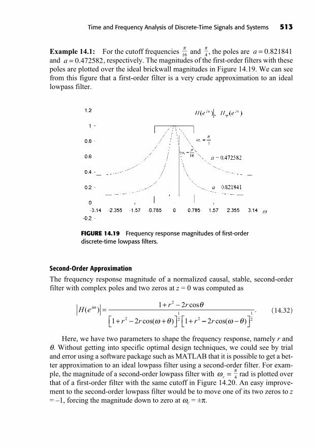
Example 14.1: For the cutoff frequencies and , the poles are and , respectively. The magnitudes of the first-order filters with thesepoles are plotted over the ideal brickwall magnitudes in Figure 14.19. We can seefrom this figure that a first-order filter is a very crude approximation to an ideallowpass filter.
a = 0 472582.a = 0 821841.416
Time and Frequency Analysis of Discrete-Time Signals and Systems 513
FIGURE 14.19 Frequency response magnitudes of first-orderdiscrete-time lowpass filters.
Second-Order Approximation
The frequency response magnitude of a normalized causal, stable, second-orderfilter with complex poles and two zeros at z = 0 was computed as
(14.32)
Here, we have two parameters to shape the frequency response, namely r and. Without getting into specific optimal design techniques, we could see by trial
and error using a software package such as MATLAB that it is possible to get a bet-ter approximation to an ideal lowpass filter using a second-order filter. For exam-ple, the magnitude of a second-order lowpass filter with is plotted overthat of a first-order filter with the same cutoff in Figure 14.20. An easy improve-ment to the second-order lowpass filter would be to move one of its two zeros to z= –1, forcing the magnitude down to zero at c = ± .
rad4c =
H er r
r r r
j( )cos
cos( )
=+
+ + +
1 2
1 2 1
2
212 2 2
12r cos( )
.
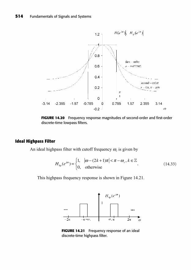
514 Fundamentals of Signals and Systems
Ideal Highpass Filter
An ideal highpass filter with cutoff frequency c is given by
(14.33)
This highpass frequency response is shown in Figure 14.21.
H ek k
hpj c( )
, ( ) ,
,=
+ <1 2 1
0
�otherwise
..
FIGURE 14.20 Frequency response magnitudes of second-order and first-orderdiscrete-time lowpass filters.
FIGURE 14.21 Frequency response of an idealdiscrete-time highpass filter.

The ideal highpass frequency response can be seen as the ideal lowpass spec-trum with cutoff frequency – c and frequency-shifted by radians. From thefrequency shifting property of the DTFT, we find that the impulse response of theideal highpass filter is:
(14.34)
Unfortunately, this highpass filter is also impossible to implement in real time,as it is noncausal and the impulse response extends to infinity both toward the neg-ative times and the positive times.
First-Order Approximation
The ideal highpass frequency response can be approximated by a normalizedcausal, stable, first-order filter with a negative pole –1 < a < 0. The normalizationis done at the highest frequency = ; that is, z = –1 so that H(–1) = 1.
(14.35)
(14.36)
Note that the relationship between the cutoff frequency c and the pole a isgiven by Equation14.31, but using the “new” pole and the “new” cutoff fre-quency – c. After is obtained from the equation, the pole of the highpass fil-ter is just a = – .
Example 14.2: The poles corresponding to the cutoff frequencies and ofa first-order highpass filter are a = –0.472582 and a = –0.821841, respectively. Thecorresponding filter magnitudes are plotted in Figure 14.22 over the ideal brickwallhighpass frequency responses.
15
16
3
4
aa
a
H ea
a aj( )
( cos ) /=+
+1
1 22 1 2
H z aaz
( ) = +( )11
1 1
h n e h n
n
n
hpj n
lp
n c
n
[ ] [ ]
( )sin( )
( )si
=
=
=
1
1nn
.cn
n
Time and Frequency Analysis of Discrete-Time Signals and Systems 515
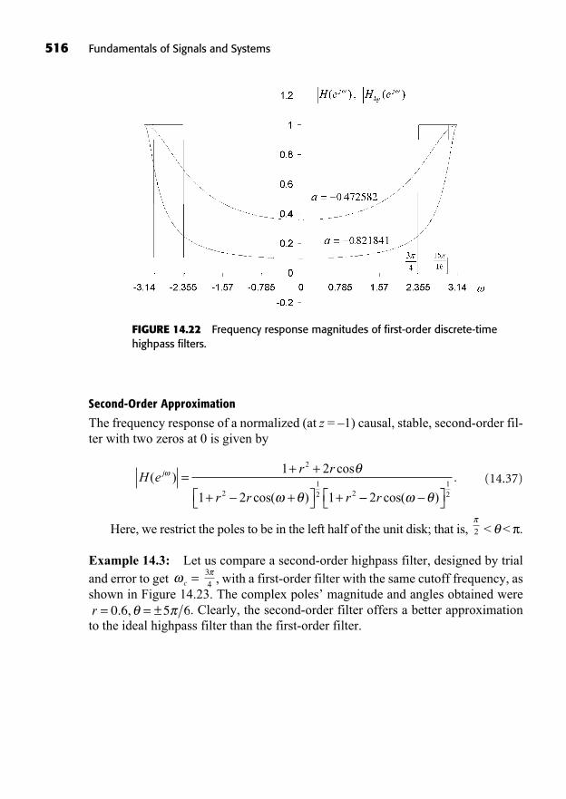
Second-Order Approximation
The frequency response of a normalized (at z = –1) causal, stable, second-order fil-ter with two zeros at 0 is given by
(14.37)
Here, we restrict the poles to be in the left half of the unit disk; that is, < < .
Example 14.3: Let us compare a second-order highpass filter, designed by trial and error to get , with a first-order filter with the same cutoff frequency, asshown in Figure 14.23. The complex poles’ magnitude and angles obtained were
. Clearly, the second-order filter offers a better approximationto the ideal highpass filter than the first-order filter.r = = ±0 6 5 6. ,
3
4c =
2
H er r
r r r
j( )cos
cos( )
=+ +
+ + +
1 2
1 2 1
2
212 2 2
12r cos( )
.
516 Fundamentals of Signals and Systems
FIGURE 14.22 Frequency response magnitudes of first-order discrete-timehighpass filters.
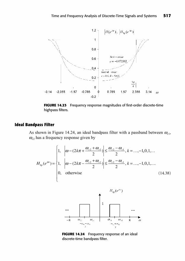
Ideal Bandpass Filter
As shown in Figure 14.24, an ideal bandpass filter with a passband between c1,c2 has a frequency response given by
(14.38)
H e
k k
bpj
c c c c
( )
, ( ) , ,
=
++
=1 22 2
12 1 2 1 … ,, , ,
, ( ) , , ,
0 1
1 22 2
1 02 1 2 1
…
…+
=k kc c c c ,, ,
,
.1
0
…
otherwise
Time and Frequency Analysis of Discrete-Time Signals and Systems 517
FIGURE 14.23 Frequency response magnitudes of first-order discrete-timehighpass filters.
FIGURE 14.24 Frequency response of an idealdiscrete-time bandpass filter.
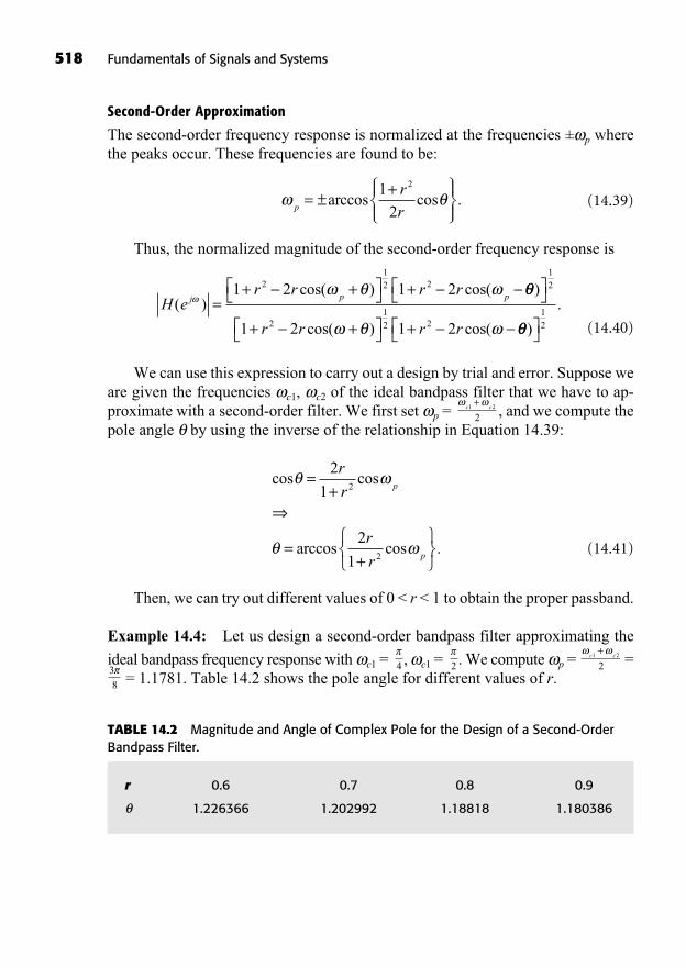
Second-Order Approximation
The second-order frequency response is normalized at the frequencies ± p wherethe peaks occur. These frequencies are found to be:
(14.39)
Thus, the normalized magnitude of the second-order frequency response is
(14.40)
We can use this expression to carry out a design by trial and error. Suppose weare given the frequencies c1, c2 of the ideal bandpass filter that we have to ap-proximate with a second-order filter. We first set p = , and we compute thepole angle by using the inverse of the relationship in Equation 14.39:
(14.41)
Then, we can try out different values of 0 < r < 1 to obtain the proper passband.
Example 14.4: Let us design a second-order bandpass filter approximating the
ideal bandpass frequency response with c1 = , c1 = . We compute p = == 1.1781. Table 14.2 shows the pole angle for different values of r.
3
8
c c+
1 2
224
cos cos
arccos cos .
=+
=+
2
1
2
1
2
2
r
r
r
r
p
p
c c+
1 2
2
H er r r r
j p p( )
cos( ) cos(=
+ + +1 2 1 2212 2 )
cos( ) cos(+ + +
12
212 21 2 1 2r r r r )
.12
p
r
r= ±
+arccos cos .
1
2
2
518 Fundamentals of Signals and Systems
r 0.6 0.7 0.8 0.9
1.226366 1.202992 1.18818 1.180386
TABLE 14.2 Magnitude and Angle of Complex Pole for the Design of a Second-OrderBandpass Filter.
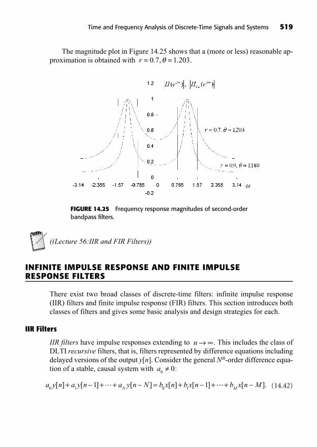
The magnitude plot in Figure 14.25 shows that a (more or less) reasonable ap-proximation is obtained with .r = =0 7 1 203. , .
Time and Frequency Analysis of Discrete-Time Signals and Systems 519
FIGURE 14.25 Frequency response magnitudes of second-orderbandpass filters.
((Lecture 56:IIR and FIR Filters))
INFINITE IMPULSE RESPONSE AND FINITE IMPULSE RESPONSE FILTERS
There exist two broad classes of discrete-time filters: infinite impulse response(IIR) filters and finite impulse response (FIR) filters. This section introduces bothclasses of filters and gives some basic analysis and design strategies for each.
IIR Filters
IIR filters have impulse responses extending to . This includes the class ofDLTI recursive filters, that is, filters represented by difference equations includingdelayed versions of the output y[n]. Consider the general Nth-order difference equa-tion of a stable, causal system with :
(14.42)a y n a y n a y n N b x n b x nN0 1 0 1
1 1[ ] [ ] [ ] [ ] [ ]+ + + = + + + b x n MM
[ ].
a0
0
n

This equation represents an IIR filter if at least one of the coefficientsis nonzero. In terms of transfer functions, IIR filters have transfer functions with atleast one pole pm different from 0:
(14.43)
The usual first-order and second-order filters are examples of IIR filters, forexample,
(14.44)
whose associated recursive difference equation is
(14.45)
We have already studied simple design methods for these types of filters (withtheir zeros restricted to be at 0) to approximate ideal filters in the previous section.There exist several approaches to design accurate high-order IIR filters. One ofthem is to design the filter in continuous time (in the Laplace domain), using, forexample, the Butterworth, Chebyshev, or elliptic pole patterns and then transform-ing the Laplace-domain transfer function into the z-domain using the bilinear trans-formation. Other computer-aided techniques use iterative optimization methodson the discrete-time filter coefficients to minimize the error between the desiredfrequency response and the filter’s actual frequency response.
Benefits of IIR filters include the following:
Low-order filters can offer relatively sharp transition bands.They have low memory requirements when implemented as a recursive equation.
y n y n x n x n[ ] [ ] [ ] [ ].= + +1
21
1
31
H zz
zz( ) , ,=
+>
113
112
1
2
1
1
H zb b z b z
a a z a z
A
MM
NN
( )( )
( )=
+ + ++ + +
=
0 11
0 11
(( )
( )
( )
1
1
1
1
1
1
=
=
=
=
z z
p z
Azz z
kk
M
kk
N
N M kk 11
1
M
kk
Nz p
=( )
.
ai i
N{ } =1
520 Fundamentals of Signals and Systems
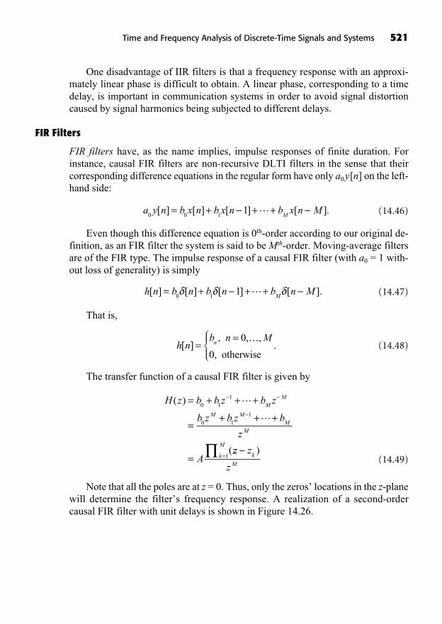
One disadvantage of IIR filters is that a frequency response with an approxi-mately linear phase is difficult to obtain. A linear phase, corresponding to a timedelay, is important in communication systems in order to avoid signal distortioncaused by signal harmonics being subjected to different delays.
FIR Filters
FIR filters have, as the name implies, impulse responses of finite duration. Forinstance, causal FIR filters are non-recursive DLTI filters in the sense that theircorresponding difference equations in the regular form have only a0y[n] on the left-hand side:
(14.46)
Even though this difference equation is 0th-order according to our original de-finition, as an FIR filter the system is said to be Mth-order. Moving-average filtersare of the FIR type. The impulse response of a causal FIR filter (with a0 = 1 with-out loss of generality) is simply
(14.47)
That is,
(14.48)
The transfer function of a causal FIR filter is given by
(14.49)
Note that all the poles are at z = 0. Thus, only the zeros’ locations in the z-planewill determine the filter’s frequency response. A realization of a second-ordercausal FIR filter with unit delays is shown in Figure 14.26.
H z b b z b z
b z b z b
z
A
MM
M MM
M
( )
(
= + + +
=+ + +
=
0 11
0 11
zz z
zkk
M
M=
)1
h nb n M
n[ ], , ,
,.=
= 0
0
…
otherwise
h n b n b n b n MM
[ ] [ ] [ ] [ ].= + + +0 1
1
a y n b x n b x n b x n MM0 0 1
1[ ] [ ] [ ] [ ].= + + +
Time and Frequency Analysis of Discrete-Time Signals and Systems 521
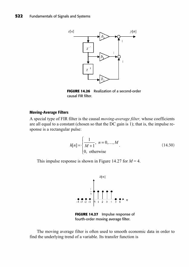
522 Fundamentals of Signals and Systems
Moving-Average Filters
A special type of FIR filter is the causal moving-average filter, whose coefficientsare all equal to a constant (chosen so that the DC gain is 1); that is, the impulse re-sponse is a rectangular pulse:
(14.50)
This impulse response is shown in Figure 14.27 for M = 4.
h n Mn M
[ ], , ,
,
.= +=
1
10
0
…
otherwise
FIGURE 14.26 Realization of a second-ordercausal FIR filter.
FIGURE 14.27 Impulse response offourth-order moving average filter.
The moving average filter is often used to smooth economic data in order tofind the underlying trend of a variable. Its transfer function is

(14.51)
The frequency response of the causal moving average filter is computed asfollows.
(14.52)
Alternatively, we can use the finite geometric sum formula in Table B.2 (Ap-pendix B) to obtain a single equivalent expression for H(ej ):
(14.53)
The magnitude of this frequency response displays M zeros, the first one being
at = , as shown in Figure 14.28. Thus, the bandwidth of this lowpass filterdepends only on its length and cannot be specified otherwise.
+2
1M
H eM
e
M
e
e
e
j j kM
j M
j
( )
( )
=+
=+
=
+
1
1
1
1
1
1
0
1
+ + +
+
jM
j
jM
jM
j jM e
e e
e e
12
2
12
12
21( )
(
2
2
1
12
2
=+
+e
M
Mj
M sin
sin
.
H eM
e e
Me e
j j j M
jM
jM
( ) =+
+ + +( )
=+
1
11
1
12 2
++ + + +
=+
e e e
Me
jM
jM
jM
( ) ( )2
12
12
1
1
=
+jM
k
M Mk M2
0
2 1
1 22
cos ( ) ,/
evven
2
1 22
0
1 2
Me
Mk M
jM
k
M
+ =
cos ( ) ,( )/
oodd
H zM
z z
M
z z
z
M
M M
M
( )
.
=+
+ + +( )=
++ + +
1
11
1
1
1
1
1
Time and Frequency Analysis of Discrete-Time Signals and Systems 523
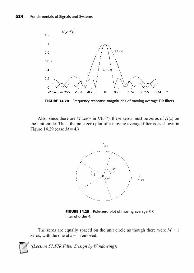
524 Fundamentals of Signals and Systems
Also, since there are M zeros in H(ej ), these zeros must be zeros of H(z) onthe unit circle. Thus, the pole-zero plot of a moving average filter is as shown inFigure 14.29 (case M = 4.)
FIGURE 14.28 Frequency response magnitudes of moving average FIR filters.
FIGURE 14.29 Pole-zero plot of moving average FIRfilter of order 4.
The zeros are equally spaced on the unit circle as though there were M + 1zeros, with the one at z = 1 removed.
((Lecture 57:FIR Filter Design by Windowing))

FIR Filter Design by Impulse Response Truncation
FIR filters can be designed via a straight truncation of a desired infinite impulseresponse. This method is very effective and popular because it is straightforward,and one can get extremely sharp transitions and linear phases, but at the cost oflong filter lengths.
Consider for example the noncausal, real, even, infinite impulse response ofthe ideal lowpass filter:
(14.54)
This impulse response is plotted in Figure 14.30 for the cutoff frequency c = .4
h nn n
nlpc c c[ ] .= =
( )sinc
sin
Time and Frequency Analysis of Discrete-Time Signals and Systems 525
FIGURE 14.30 Impulse response of ideal lowpass IIR filter.
A first attempt would be to truncate this response and keep only the first M +1 values of the causal part. However, this does not produce very good results. Fora given filter length M + 1 and assuming that M is even, it is much better to time-delay the impulse response by M/2 first and then truncate it to retain only the val-ues for .
Example 14.5: Suppose we select M = 40, and we want to have a cutoff fre-quency of c = . Then, we delay the impulse response shown above by 20 timesteps and truncate it to obtain the finite impulse response h[n] = hlp[n – 20](u[n] –u[n – 41]) shown in Figure 14.31.
4
n M= 0, ,…
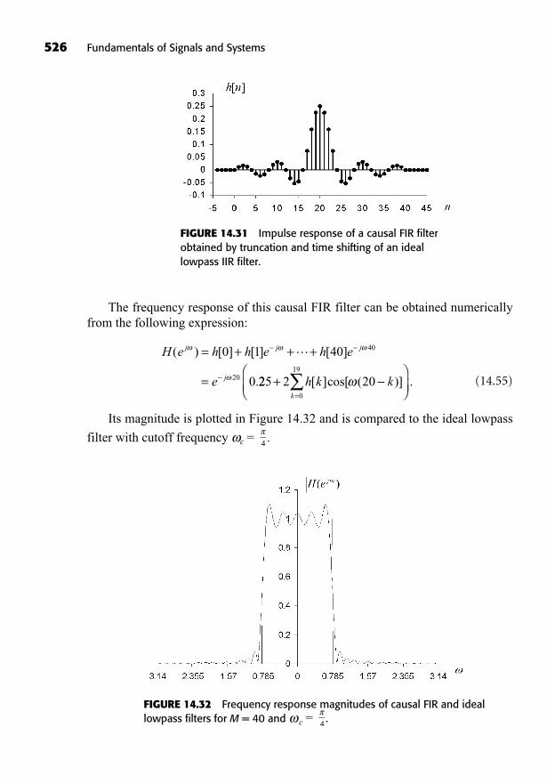
526 Fundamentals of Signals and Systems
The frequency response of this causal FIR filter can be obtained numericallyfrom the following expression:
(14.55)
Its magnitude is plotted in Figure 14.32 and is compared to the ideal lowpass
filter with cutoff frequency c = .4
H e h h e h e
e
j j j
j
( ) [ ] [ ] [ ]
.
= + + +
=
0 1 40
0
40
20
225 2 200
19
+=
h k kk
[ ]cos[ ( )] .
FIGURE 14.31 Impulse response of a causal FIR filterobtained by truncation and time shifting of an ideallowpass IIR filter.
FIGURE 14.32 Frequency response magnitudes of causal FIR and ideallowpass filters for M = 40 and c = .4
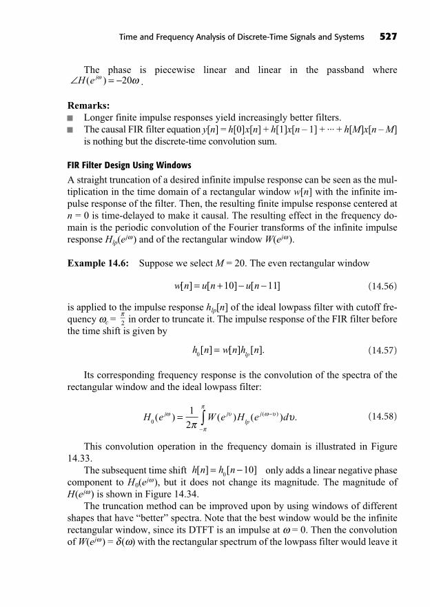
The phase is piecewise linear and linear in the passband where.
Remarks:Longer finite impulse responses yield increasingly better filters.The causal FIR filter equation y[n] = h[0]x[n] + h[1]x[n – 1] + ... + h[M]x[n – M]is nothing but the discrete-time convolution sum.
FIR Filter Design Using Windows
A straight truncation of a desired infinite impulse response can be seen as the mul-tiplication in the time domain of a rectangular window w[n] with the infinite im-pulse response of the filter. Then, the resulting finite impulse response centered atn = 0 is time-delayed to make it causal. The resulting effect in the frequency do-main is the periodic convolution of the Fourier transforms of the infinite impulseresponse Hlp(ej ) and of the rectangular window W(ej ).
Example 14.6: Suppose we select M = 20. The even rectangular window
(14.56)
is applied to the impulse response hlp[n] of the ideal lowpass filter with cutoff fre-quency c = in order to truncate it. The impulse response of the FIR filter beforethe time shift is given by
(14.57)
Its corresponding frequency response is the convolution of the spectra of therectangular window and the ideal lowpass filter:
(14.58)
This convolution operation in the frequency domain is illustrated in Figure14.33.
The subsequent time shift only adds a linear negative phasecomponent to H0(ej ), but it does not change its magnitude. The magnitude ofH(ej ) is shown in Figure 14.34.
The truncation method can be improved upon by using windows of differentshapes that have “better” spectra. Note that the best window would be the infiniterectangular window, since its DTFT is an impulse at = 0. Then the convolutionof W(ej ) = ( ) with the rectangular spectrum of the lowpass filter would leave it
h n h n[ ] [ ]=0
10
H e W e H e dj jlp
j0
1
2( ) ( ) ( ) .( )=
h n w n h nlp0
[ ] [ ] [ ].=
2
w n u n u n[ ] [ ] [ ]= +10 11
=H e j( ) 20
Time and Frequency Analysis of Discrete-Time Signals and Systems 527
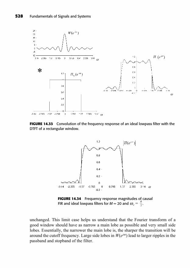
unchanged. This limit case helps us understand that the Fourier transform of agood window should have as narrow a main lobe as possible and very small sidelobes. Essentially, the narrower the main lobe is, the sharper the transition will bearound the cutoff frequency. Large side lobes in W(ej ) lead to larger ripples in thepassband and stopband of the filter.
528 Fundamentals of Signals and Systems
FIGURE 14.33 Convolution of the frequency response of an ideal lowpass filter with theDTFT of a rectangular window.
FIGURE 14.34 Frequency response magnitudes of causalFIR and ideal lowpass filters for M = 20 and c = .2
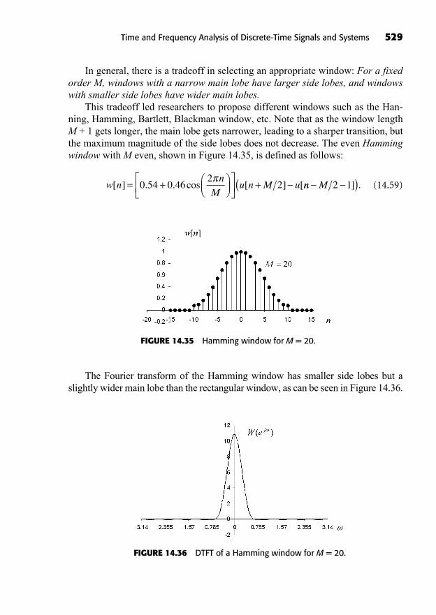
In general, there is a tradeoff in selecting an appropriate window: For a fixedorder M, windows with a narrow main lobe have larger side lobes, and windowswith smaller side lobes have wider main lobes.
This tradeoff led researchers to propose different windows such as the Han-ning, Hamming, Bartlett, Blackman window, etc. Note that as the window lengthM + 1 gets longer, the main lobe gets narrower, leading to a sharper transition, butthe maximum magnitude of the side lobes does not decrease. The even Hammingwindow with M even, shown in Figure 14.35, is defined as follows:
(14.59)w nn
Mu n M u[ ] . . cos [ ] [= + +0 54 0 46
22 nn M( )2 1] .
Time and Frequency Analysis of Discrete-Time Signals and Systems 529
FIGURE 14.35 Hamming window for M = 20.
The Fourier transform of the Hamming window has smaller side lobes but aslightly wider main lobe than the rectangular window, as can be seen in Figure 14.36.
FIGURE 14.36 DTFT of a Hamming window for M = 20.
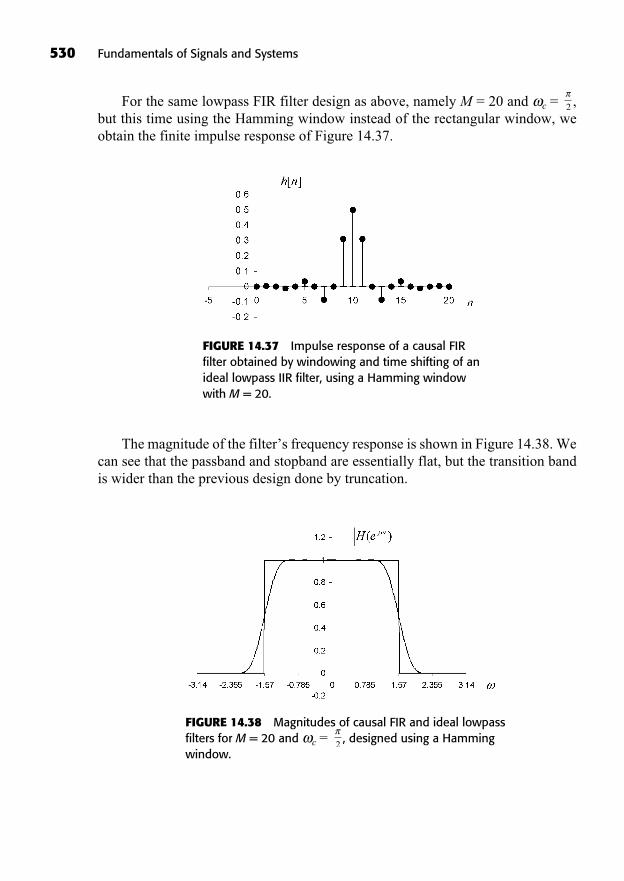
530 Fundamentals of Signals and Systems
For the same lowpass FIR filter design as above, namely M = 20 and c = ,but this time using the Hamming window instead of the rectangular window, weobtain the finite impulse response of Figure 14.37.
2
FIGURE 14.37 Impulse response of a causal FIRfilter obtained by windowing and time shifting of anideal lowpass IIR filter, using a Hamming windowwith M = 20.
The magnitude of the filter’s frequency response is shown in Figure 14.38. Wecan see that the passband and stopband are essentially flat, but the transition bandis wider than the previous design done by truncation.
FIGURE 14.38 Magnitudes of causal FIR and ideal lowpassfilters for M = 20 and c = , designed using a Hammingwindow.
2
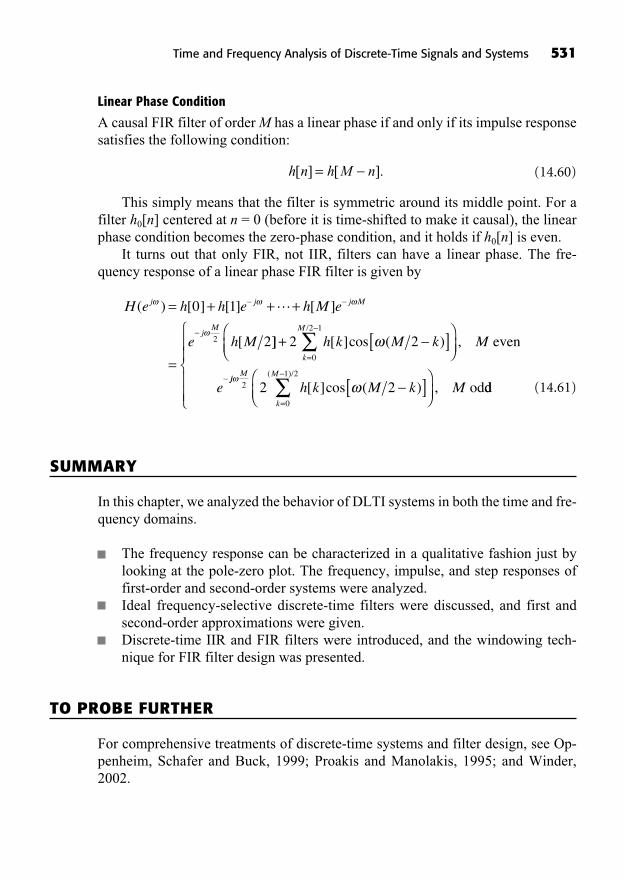
Linear Phase Condition
A causal FIR filter of order M has a linear phase if and only if its impulse responsesatisfies the following condition:
(14.60)
This simply means that the filter is symmetric around its middle point. For afilter h0[n] centered at n = 0 (before it is time-shifted to make it causal), the linearphase condition becomes the zero-phase condition, and it holds if h0[n] is even.
It turns out that only FIR, not IIR, filters can have a linear phase. The fre-quency response of a linear phase FIR filter is given by
(14.61)
SUMMARY
In this chapter, we analyzed the behavior of DLTI systems in both the time and fre-quency domains.
The frequency response can be characterized in a qualitative fashion just bylooking at the pole-zero plot. The frequency, impulse, and step responses offirst-order and second-order systems were analyzed.Ideal frequency-selective discrete-time filters were discussed, and first andsecond-order approximations were given.Discrete-time IIR and FIR filters were introduced, and the windowing tech-nique for FIR filter design was presented.
TO PROBE FURTHER
For comprehensive treatments of discrete-time systems and filter design, see Op-penheim, Schafer and Buck, 1999; Proakis and Manolakis, 1995; and Winder,2002.
H e h h e h M e
e h M
j j j M
jM
( ) [ ] [ ] [ ]
[
= + + +
=
0 1
22
]] [ ]cos ( ) ,/
+ [ ]=
2 20
2 1
h k M k M
e
k
M
even
jjM
k
M
h k M k M2
0
1 2
2 2[ ]cos ( ) ,( )/
=[ ] oddd
h n h M n[ ] [ ].=
Time and Frequency Analysis of Discrete-Time Signals and Systems 531

EXERCISES
Exercises with Solutions
Exercise 14.1
(a) Design a discrete-time second-order IIR bandpass filter approximating the
ideal bandpass filter with frequencies and normalize itto have a passband-frequency gain of 1.
Answer:We compute . The pole angle is independent of r, as
The transfer function is
The magnitude plot in Figure 14.39 shows that a “reasonable” design is ob-tained with r = 0.52.
(b) Plot the magnitude of its frequency response and the magnitude of theideal bandpass filter on the same graph.
Answer:The frequency response magnitudes of the bandpass filters are plotted in Figure14.39.
H zr r r r
p p( )
cos( ) cos( )=
+ + +1 2 1 2212 2
+>
=+
12
1 2 2
2
1 2
1 2
r z r zz r
r r
cos,
cos( ) +
+
12 2
12
1 2 2
1 2 0
1 22
r r
r z r z
cos( )
cos,,
(
z r
r r r r
r z
>
=+ + +
+=
+1 2 1 2
1
1212 2
12
2 2
rr r
r z
r
r zz r
2 2 2
2 2
2 2
2 2
4
1
1
1
) ( ), .
+=
+>
=+
= { } =arccos cos arccos .2
10
22
r
r p
=2
=c c+1 2
2p =
3
4c2 =,4c1 =
532 Fundamentals of Signals and Systems
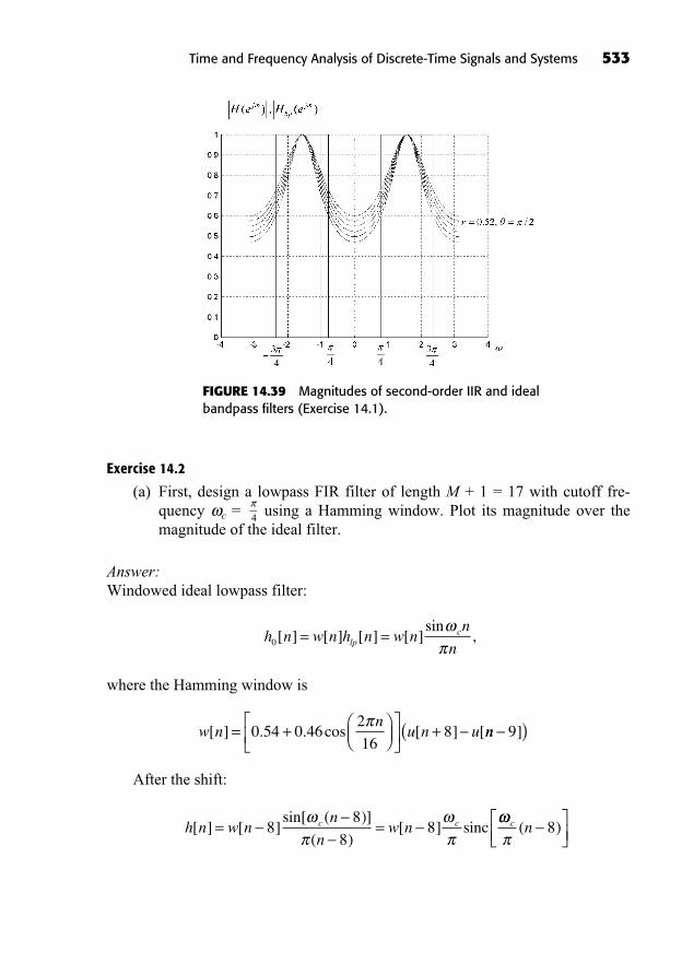
Exercise 14.2
(a) First, design a lowpass FIR filter of length M + 1 = 17 with cutoff fre-quency c = using a Hamming window. Plot its magnitude over themagnitude of the ideal filter.
Answer:Windowed ideal lowpass filter:
where the Hamming window is
After the shift:
h n w nn
nw nc c[ ] [ ]
sin[ ( )]
( )[ ]= =8
8
88 sinc c n( )8
w nn
u n u[ ] . . cos [ ] [= + +0 54 0 462
168 nn( )9]
h n w n h n w nn
nlpc
0[ ] [ ] [ ] [ ]sin
,= =
4
Time and Frequency Analysis of Discrete-Time Signals and Systems 533
FIGURE 14.39 Magnitudes of second-order IIR and idealbandpass filters (Exercise 14.1).
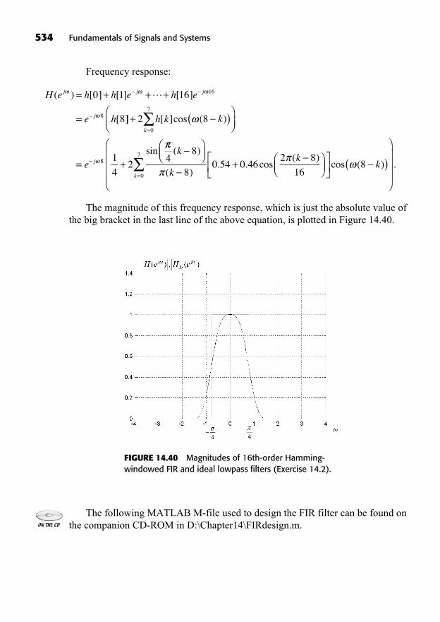
534 Fundamentals of Signals and Systems
Frequency response:
The magnitude of this frequency response, which is just the absolute value ofthe big bracket in the last line of the above equation, is plotted in Figure 14.40.
H e h h e h e
e h
j j j
j
( ) [ ] [ ] [ ]
[
= + + +
=
0 1 16
8
16
8
]] [ ]cos ( )
sin
+ ( )
= +
=
2 8
1
42
0
7
8
h k k
e
k
j 48
80 54 0 46
2 8
16
( )
( ). . cos
( )k
k
k+ ( )
=
cos ( ) .k
k0
7
8
FIGURE 14.40 Magnitudes of 16th-order Hamming-windowed FIR and ideal lowpass filters (Exercise 14.2).
The following MATLAB M-file used to design the FIR filter can be found onthe companion CD-ROM in D:\Chapter14\FIRdesign.m.
%% Freq resp of FIR filter
% number of points in FIR filter is M+1
M=16;
% cutoff frequency of lowpass
wc=pi/4;
% freq vector
w=[-pi:0.01:pi]’;
% FR computation using cosine formula
Hjw=(wc/pi)*ones(length(w),1);
for k=0:M/2-1
Hjw=Hjw+2*sin((k-M/2)*wc)/((k-M/2)*pi)*(0.54+0.46*cos(2*pi*(k-
M/2)/M))*cos(w*(M/2-k));
end
% Ideal lowpass
Hlp=zeros(length(w),1);
for k=1:length(w)
if (abs(w(k)) < wc)
Hlp(k)=1;
end
end
%plot frequency response
plot(w,abs(Hjw),w,Hlp);
(b) Use the filter in (a) to form a real bandpass FIR filter with cutoff frequen-
cies . Give its impulse response and plot its magnitude over the mag-nitude of the ideal bandpass filter and that of the IIR filter in Exercise 14.1.
Answer:Using frequency shifting,
H e H e H e
h h e
j j j
12 2
0 1
( ) ( ) ( )
[ ] [ ]
( ) ( )= +
= +
+
jj jh e h h
( ) ( )[ ] [ ] [ ]
+ ++ + + +2 2
1616 0 1 ee h e
h
j j+ +
= +
( ) ( )[ ]
[ ] (
2 216
16
2 0
ee e h k e
h
j k j k jk
k=
+
= +
2 2
1
16
2 0 22
) [ ]
[ ] cos( kk h k e jk
k
) [ ] .=1
16
4
3
4,
Time and Frequency Analysis of Discrete-Time Signals and Systems 535
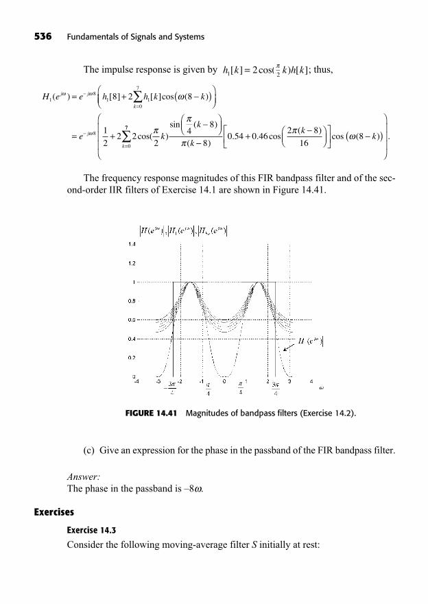
536 Fundamentals of Signals and Systems
The impulse response is given by ; thus,
The frequency response magnitudes of this FIR bandpass filter and of the sec-ond-order IIR filters of Exercise 14.1 are shown in Figure 14.41.
H e e h h k kj j
k1
81 1
0
7
8 2 8( ) [ ] [ ]cos ( )= + ( )=
= +e kk
kj 8 1
22 2
24
8cos( )
sin ( )
(+
= 80 54 0 46
2 8
160 ). . cos
( )cos
k
k
77
8( )( ) .k
k h k) [ ]2
(h k1 2[ ] cos(=
FIGURE 14.41 Magnitudes of bandpass filters (Exercise 14.2).
(c) Give an expression for the phase in the passband of the FIR bandpass filter.
Answer:The phase in the passband is –8 .
Exercises
Exercise 14.3
Consider the following moving-average filter S initially at rest:
S: .
(a) Find the impulse response h[n] of the filter. Is it causal?
(b) Find the transfer function of the filter H(z) and give its region of conver-gence. Sketch the pole-zero plot.
(c) Find the frequency response of the filter. Sketch its magnitude.
(d) Compute the 3 dB cutoff frequency c.
Answer:
Exercise 14.4
Suppose we want to design a causal, stable, first-order highpass filter of the type
with 3 dB cutoff frequency c = and a real.(a) Express the real constant B in terms of the pole a to obtain unity gain at the
highest frequency = .
(b) Design the filter; that is, find the numerical values of the pole a and theconstant B.
(c) Sketch the magnitude of the filter’s frequency response.
Exercise 14.5
(a) Design a discrete-time second-order IIR lowpass filter approximating theideal lowpass filter with –3 dB cutoff frequency c = and normalize itto have a DC gain of 1. You can proceed by trial and error. Plot the mag-nitude of its frequency response (use MATLAB) and the magnitude of theideal lowpass filter on the same figure.
(b) Add a zero at = to your design to improve the response at high fre-quency. Plot the resulting frequency response magnitude as well as the re-sponse in (a) and discuss the results.
Answer:
6
2
3
H zB
azz a( ) ,= >
1 1
y n x n x n x n x n[ ] [ ] [ ] [ ] [ ]= + + + +1
41
1
4
1
41
1
42
Time and Frequency Analysis of Discrete-Time Signals and Systems 537

538 Fundamentals of Signals and Systems
Exercise 14.6
(a) First, design a lowpass FIR filter of order M = 256 with cutoff frequency
c = radians using a Hamming window. Plot its magnitude over themagnitudes of the ideal filter and the filters in Exercise 14.5.
(b) Give an expression for the phase in the passband of the FIR bandpass filter.
(c) Simulate the filter for the input until theoutput reaches steady-state and plot the results. Also plot the input on aseparate graph.
Exercise 14.7
(a) Design a first-order discrete-time lowpass filter with a 3 dB cutoff fre-quency c = and a DC gain of 1.
(b) Plot the magnitude of its frequency response.
(c) Write the filter as a difference equation and plot the first 20 values of thefiltered signal y[n] for the input signal with thefilter being initially at rest.
Answer:
Exercise 14.8
(a) Design a DT second-order IIR bandpass filter approximating the ideal
bandpass filter with frequencies and normalize it tohave a passband-frequency gain of 5.
(b) Plot the magnitude of its frequency response and the magnitude of theideal bandpass filter on the same figure.
Exercise 14.9
(a) Design a first-order DT lowpass filter with a –3 dB cutoff frequency
c = and a DC gain of 1.
(b) Plot the magnitude of its frequency response.
(c) Write the filter as a difference equation, and plot the first 15 values of thefiltered signal y[n] for the input signal .x n u n[ ] [ ]= 2
12
2c2 =,3
8=c1 =
x n u n u n[ ] [ ] [ ]= 10
12
x n n u n n u n[ ] cos( ) [ ] cos( ) [ ]= +8 4
6

Time and Frequency Analysis of Discrete-Time Signals and Systems 539
Answer:
Exercise 14.10
(a) Design a 20th-order (i.e., M = 20) DT causal FIR highpass filter approxi-
mating the ideal highpass filter with c = and normalized to have ahigh-frequency gain of 1. Use the straight truncation (rectangular window)technique.
(b) Repeat (a) using the Hamming window.
(c) Plot the magnitudes of the frequency responses of the two FIR filters, themagnitude of the IIR filter obtained in Exercise 14.4, and the magnitude ofthe ideal highpass filter on the same figure.
(d) Plot the first 20 values of the two filtered signals y[n], i.e., the output ofeach filter, for the step input signal x[n] = u[n].
2
3

This page intentionally left blank
541
Sampling Systems15
((Lecture 58: Sampling))
This chapter introduces the important bridge between continuous-time anddiscrete-time signals provided by the sampling process. Sampling recordsdiscrete values of a continuous-time signal at periodic instants of time, either
for real-time processing or for storage and subsequent off-line processing. Sam-pling opens up a world of possibilities for the processing of continuous-time sig-nals through the use of discrete-time systems such as infinite impulse response(IIR) and finite impulse response (FIR) filters.
In This Chapter
Sampling of Continuous-Time SignalsSignal ReconstructionDiscrete-Time Processing of Continuous-Time SignalsSampling of Discrete-Time SignalsSummaryTo Probe FurtherExercises
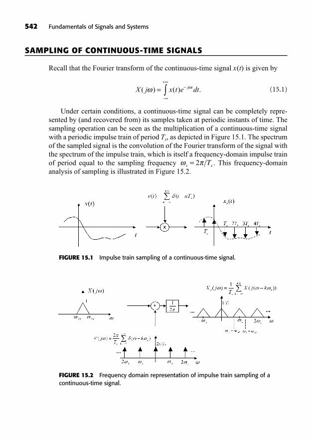
542 Fundamentals of Signals and Systems
SAMPLING OF CONTINUOUS-TIME SIGNALS
Recall that the Fourier transform of the continuous-time signal x(t) is given by
(15.1)
Under certain conditions, a continuous-time signal can be completely repre-sented by (and recovered from) its samples taken at periodic instants of time. Thesampling operation can be seen as the multiplication of a continuous-time signalwith a periodic impulse train of period Ts, as depicted in Figure 15.1. The spectrumof the sampled signal is the convolution of the Fourier transform of the signal withthe spectrum of the impulse train, which is itself a frequency-domain impulse trainof period equal to the sampling frequency . This frequency-domainanalysis of sampling is illustrated in Figure 15.2.
s sT= 2
X j x t e dtj t( ) ( ) .=+
FIGURE 15.1 Impulse train sampling of a continuous-time signal.
FIGURE 15.2 Frequency domain representation of impulse train sampling of acontinuous-time signal.
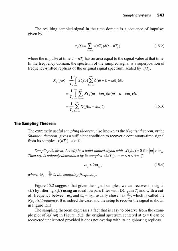
The resulting sampled signal in the time domain is a sequence of impulsesgiven by
(15.2)
where the impulse at time has an area equal to the signal value at that time.In the frequency domain, the spectrum of the sampled signal is a superposition offrequency-shifted replicas of the original signal spectrum, scaled by .
(15.3)
The Sampling Theorem
The extremely useful sampling theorem, also known as the Nyquist theorem, or theShannon theorem, gives a sufficient condition to recover a continuous-time signalfrom its samples .
Sampling theorem: Let x(t) be a band-limited signal with .Then x(t) is uniquely determined by its samples if
(15.4)
where is the sampling frequency.
Figure 15.2 suggests that given the signal samples, we can recover the signalx(t) by filtering xs(t) using an ideal lowpass filter with DC gain Ts and with a cut-off frequency between M and s – M, usually chosen as , which is called theNyquist frequency. It is indeed the case, and the setup to recover the signal is shownin Figure 15.3.
The sampling theorem expresses a fact that is easy to observe from the exam-ple plot of Xs( j ) in Figure 15.2: the original spectrum centered at = 0 can berecovered undistorted provided it does not overlap with its neighboring replicas.
s
2
sT
2s =
s M> 2 ,
x nT ns( ), < < +X j
M( ) = >0 for
x nT ns( ), �
X jT
X j k d
T
ss
sk
s
( ) ( ) ( )=
=
=
++1
1XX j k k d
TX j
s sk
s
( ( )) ( )
(=
=
++
1(( ))
=
+
k sk
1 Ts
t nTs=
x t x nT t nTs s sn
( ) ( ) ( ),==
+
Sampling Systems 543
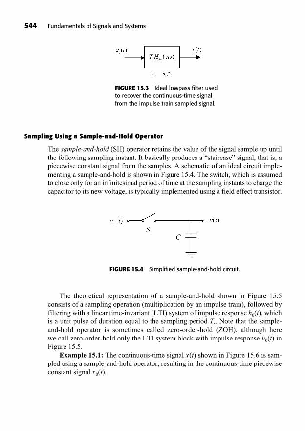
544 Fundamentals of Signals and Systems
Sampling Using a Sample-and-Hold Operator
The sample-and-hold (SH) operator retains the value of the signal sample up untilthe following sampling instant. It basically produces a “staircase” signal, that is, apiecewise constant signal from the samples. A schematic of an ideal circuit imple-menting a sample-and-hold is shown in Figure 15.4. The switch, which is assumedto close only for an infinitesimal period of time at the sampling instants to charge thecapacitor to its new voltage, is typically implemented using a field effect transistor.
FIGURE 15.3 Ideal lowpass filter usedto recover the continuous-time signalfrom the impulse train sampled signal.
FIGURE 15.4 Simplified sample-and-hold circuit.
The theoretical representation of a sample-and-hold shown in Figure 15.5consists of a sampling operation (multiplication by an impulse train), followed byfiltering with a linear time-invariant (LTI) system of impulse response h0(t), whichis a unit pulse of duration equal to the sampling period Ts. Note that the sample-and-hold operator is sometimes called zero-order-hold (ZOH), although here we call zero-order-hold only the LTI system block with impulse response h0(t) inFigure 15.5.
Example 15.1: The continuous-time signal x(t) shown in Figure 15.6 is sam-pled using a sample-and-hold operator, resulting in the continuous-time piecewiseconstant signal x0(t).

Note that the sampled signal x0(t) carries the same information as the samplesthemselves, so according to the sampling theorem, we should be able to recover theentire signal x(t). It is indeed the case. From the block diagram of the sample-and-hold, what we would need to do is find the inverse of the ZOH system with impulseresponse h0(t) and then use a perfect lowpass filter. The frequency response H0( j )is given by the usual sinc function for an even rectangular pulse signal, multiplied
by because of the time delay of Ts/2 seconds to make the pulse causal:
(15.5)
The inverse of H0( j ) is given by
(15.6)
The reconstruction filter is the cascade of the inverse filter and the lowpass filter,
(15.7)
whose magnitude and phase are sketched in Figure 15.8.
H j T H j H jr s lp( ) : ( ) ( ),= 1
H j H j ejT
T
s
s1 01 2
2
1
2( ) ( )
sin( ).= =
H j T eT
es
jT
s jTs s
02 2
22( )
sin= =sinc
(( ).
Ts2
ejTs2
Sampling Systems 545
FIGURE 15.5 Sample-and-hold operator.
FIGURE 15.6 Effect of sample-and-hold operator on an input signal.
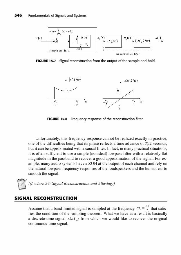
546 Fundamentals of Signals and Systems
Unfortunately, this frequency response cannot be realized exactly in practice,one of the difficulties being that its phase reflects a time advance of Ts/2 seconds,but it can be approximated with a causal filter. In fact, in many practical situations,it is often sufficient to use a simple (nonideal) lowpass filter with a relatively flatmagnitude in the passband to recover a good approximation of the signal. For ex-ample, many audio systems have a ZOH at the output of each channel and rely onthe natural lowpass frequency responses of the loudspeakers and the human ear tosmooth the signal.
((Lecture 59: Signal Reconstruction and Aliasing))
SIGNAL RECONSTRUCTION
Assume that a band-limited signal is sampled at the frequency that satis-fies the condition of the sampling theorem. What we have as a result is basically a discrete-time signal from which we would like to recover the originalcontinuous-time signal.
x nTs( )
sT=
2s =
FIGURE 15.7 Signal reconstruction from the output of the sample-and-hold.
FIGURE 15.8 Frequency response of the reconstruction filter.
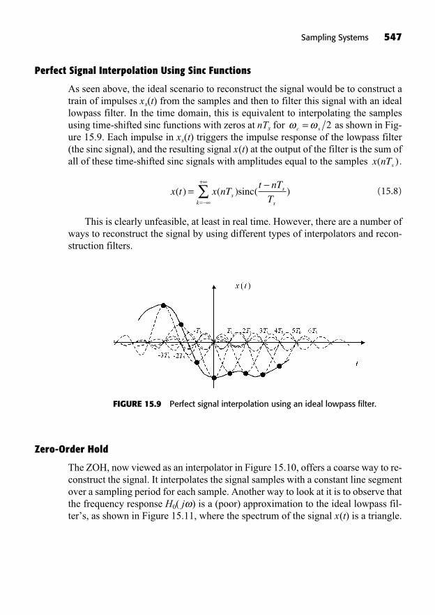
Perfect Signal Interpolation Using Sinc Functions
As seen above, the ideal scenario to reconstruct the signal would be to construct atrain of impulses xs(t) from the samples and then to filter this signal with an ideallowpass filter. In the time domain, this is equivalent to interpolating the samplesusing time-shifted sinc functions with zeros at nTs for as shown in Fig-ure 15.9. Each impulse in xs(t) triggers the impulse response of the lowpass filter(the sinc signal), and the resulting signal x(t) at the output of the filter is the sum ofall of these time-shifted sinc signals with amplitudes equal to the samples .
(15.8)
This is clearly unfeasible, at least in real time. However, there are a number ofways to reconstruct the signal by using different types of interpolators and recon-struction filters.
x t x nTt nT
Tss
sk
( ) ( ) ( )==
+
sinc
x nTs( )
c s= 2
Sampling Systems 547
FIGURE 15.9 Perfect signal interpolation using an ideal lowpass filter.
Zero-Order Hold
The ZOH, now viewed as an interpolator in Figure 15.10, offers a coarse way to re-construct the signal. It interpolates the signal samples with a constant line segmentover a sampling period for each sample. Another way to look at it is to observe thatthe frequency response H0( j ) is a (poor) approximation to the ideal lowpass fil-ter’s, as shown in Figure 15.11, where the spectrum of the signal x(t) is a triangle.
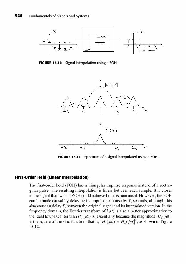
548 Fundamentals of Signals and Systems
First-Order Hold (Linear Interpolation)
The first-order hold (FOH) has a triangular impulse response instead of a rectan-gular pulse. The resulting interpolation is linear between each sample. It is closerto the signal than what a ZOH could achieve but it is noncausal. However, the FOHcan be made causal by delaying its impulse response by Ts seconds, although thisalso causes a delay Ts between the original signal and its interpolated version. In thefrequency domain, the Fourier transform of h1(t) is also a better approximation tothe ideal lowpass filter than H0( j ) is, essentially because the magnitude is the square of the sinc function; that is, , as shown in Figure15.12.
H j H j1 0
2( ) ( )=
H j1( )
FIGURE 15.10 Signal interpolation using a ZOH.
FIGURE 15.11 Spectrum of a signal interpolated using a ZOH.
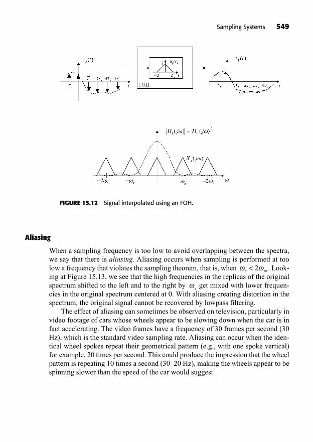
Sampling Systems 549
Aliasing
When a sampling frequency is too low to avoid overlapping between the spectra,we say that there is aliasing. Aliasing occurs when sampling is performed at toolow a frequency that violates the sampling theorem, that is, when . Look-ing at Figure 15.13, we see that the high frequencies in the replicas of the originalspectrum shifted to the left and to the right by get mixed with lower frequen-cies in the original spectrum centered at 0. With aliasing creating distortion in thespectrum, the original signal cannot be recovered by lowpass filtering.
The effect of aliasing can sometimes be observed on television, particularly invideo footage of cars whose wheels appear to be slowing down when the car is infact accelerating. The video frames have a frequency of 30 frames per second (30Hz), which is the standard video sampling rate. Aliasing can occur when the iden-tical wheel spokes repeat their geometrical pattern (e.g., with one spoke vertical)for example, 20 times per second. This could produce the impression that the wheelpattern is repeating 10 times a second (30–20 Hz), making the wheels appear to bespinning slower than the speed of the car would suggest.
s
s m< 2
FIGURE 15.12 Signal interpolated using an FOH.
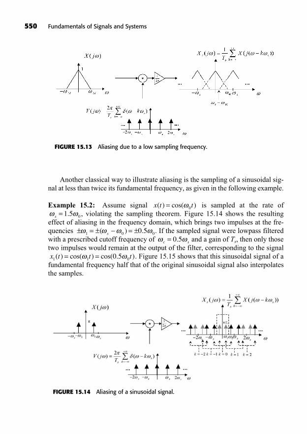
550 Fundamentals of Signals and Systems
FIGURE 15.13 Aliasing due to a low sampling frequency.
Another classical way to illustrate aliasing is the sampling of a sinusoidal sig-nal at less than twice its fundamental frequency, as given in the following example.
Example 15.2: Assume signal is sampled at the rate of, violating the sampling theorem. Figure 15.14 shows the resulting
effect of aliasing in the frequency domain, which brings two impulses at the fre-quencies . If the sampled signal were lowpass filteredwith a prescribed cutoff frequency of and a gain of Ts, then only thosetwo impulses would remain at the output of the filter, corresponding to the signal
. Figure 15.15 shows that this sinusoidal signal of afundamental frequency half that of the original sinusoidal signal also interpolatesthe samples.
x t t t1 1 00 5( ) cos( ) cos( . )= =
c s= 0 5.± = ± = ±1 0 00 5( ) .s
s = 1 5 0.x t t( ) cos( )= 0
FIGURE 15.14 Aliasing of a sinusoidal signal.
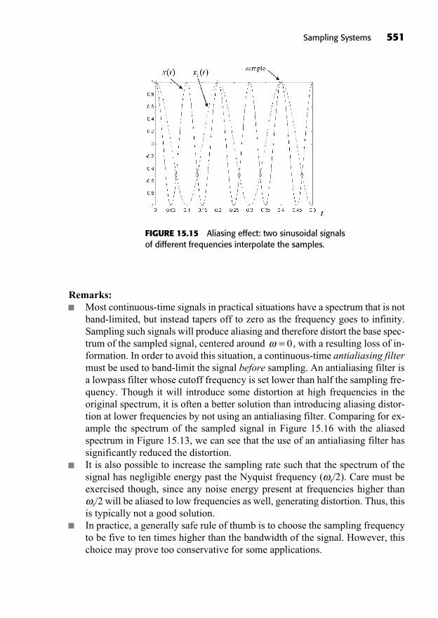
Remarks:Most continuous-time signals in practical situations have a spectrum that is notband-limited, but instead tapers off to zero as the frequency goes to infinity.Sampling such signals will produce aliasing and therefore distort the base spec-trum of the sampled signal, centered around , with a resulting loss of in-formation. In order to avoid this situation, a continuous-time antialiasing filtermust be used to band-limit the signal before sampling. An antialiasing filter isa lowpass filter whose cutoff frequency is set lower than half the sampling fre-quency. Though it will introduce some distortion at high frequencies in theoriginal spectrum, it is often a better solution than introducing aliasing distor-tion at lower frequencies by not using an antialiasing filter. Comparing for ex-ample the spectrum of the sampled signal in Figure 15.16 with the aliasedspectrum in Figure 15.13, we can see that the use of an antialiasing filter hassignificantly reduced the distortion.It is also possible to increase the sampling rate such that the spectrum of thesignal has negligible energy past the Nyquist frequency ( s/2). Care must beexercised though, since any noise energy present at frequencies higher than
s/2 will be aliased to low frequencies as well, generating distortion. Thus, thisis typically not a good solution.In practice, a generally safe rule of thumb is to choose the sampling frequencyto be five to ten times higher than the bandwidth of the signal. However, thischoice may prove too conservative for some applications.
= 0
Sampling Systems 551
FIGURE 15.15 Aliasing effect: two sinusoidal signalsof different frequencies interpolate the samples.
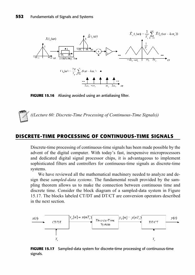
552 Fundamentals of Signals and Systems
((Lecture 60: Discrete-Time Processing of Continuous-Time Signals))
DISCRETE-TIME PROCESSING OF CONTINUOUS-TIME SIGNALS
Discrete-time processing of continuous-time signals has been made possible by theadvent of the digital computer. With today’s fast, inexpensive microprocessorsand dedicated digital signal processor chips, it is advantageous to implementsophisticated filters and controllers for continuous-time signals as discrete-timesystems.
We have reviewed all the mathematical machinery needed to analyze and de-sign these sampled-data systems. The fundamental result provided by the sam-pling theorem allows us to make the connection between continuous time anddiscrete time. Consider the block diagram of a sampled-data system in Figure15.17. The blocks labeled CT/DT and DT/CT are conversion operators describedin the next section.
FIGURE 15.16 Aliasing avoided using an antialiasing filter.
FIGURE 15.17 Sampled-data system for discrete-time processing of continuous-timesignals.

CT/DT Operator
As indicated in Figure 15.17, the continuous-time to discrete-time operator CT/DTis simply defined by
CT/DT: (15.9)
It is also useful to think of the CT/DT operator as impulse train sampling fol-lowed by a conversion of the impulse areas to values of a discrete-time signal rep-resented by the operator in Figure 15.18. To be fancy, operator , which mapsthe set of impulse-sampled signals into the set of discrete-time signals , canbe defined as follows:
(15.10)
Note that the information is the same in both representations xs(t) and ofthe sampled signal, as suggested by Figure 15.19.
x nd[ ]
V X X: , [ ] ( ) , .s d d s
nTT
nTT
x n x t dt n
ss
ss
=+
2
2
Z
XdXs
VV
x n x nT nd s[ ] ( ), .= Z
Sampling Systems 553
FIGURE 15.18 CT/DT conversion operator.
FIGURE 15.19 Impulse train sampled signal and its discrete-time counterpart in theCT/DT operation.
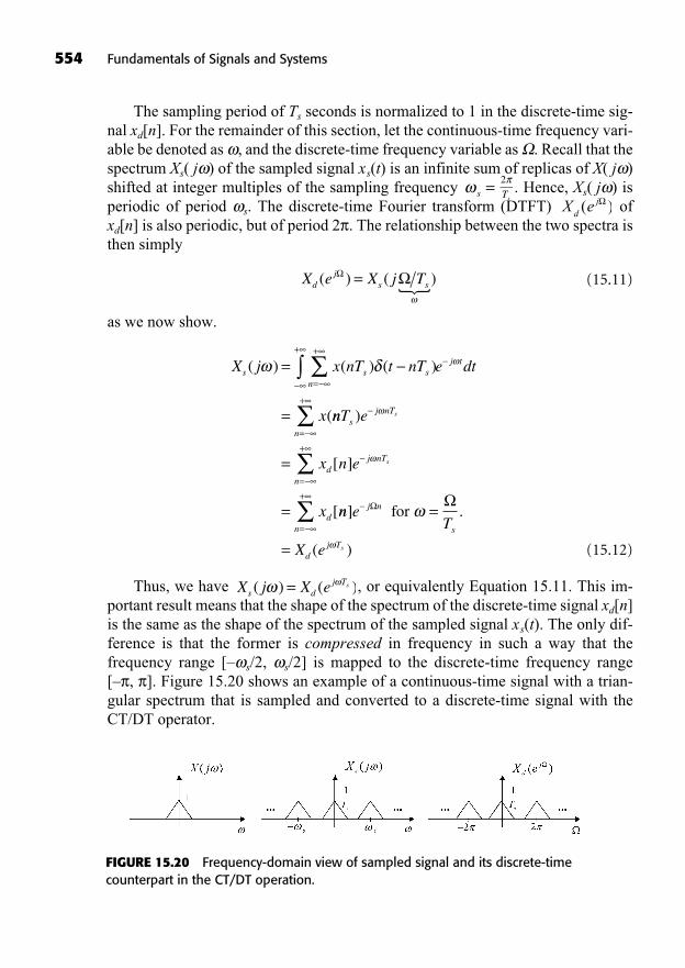
554 Fundamentals of Signals and Systems
The sampling period of Ts seconds is normalized to 1 in the discrete-time sig-nal xd[n]. For the remainder of this section, let the continuous-time frequency vari-able be denoted as , and the discrete-time frequency variable as . Recall that thespectrum Xs( j ) of the sampled signal xs(t) is an infinite sum of replicas of X( j )shifted at integer multiples of the sampling frequency . Hence, Xs( j ) isperiodic of period s. The discrete-time Fourier transform (DTFT) ofxd[n] is also periodic, but of period 2 . The relationship between the two spectra isthen simply
(15.11)
as we now show.
(15.12)
Thus, we have , or equivalently Equation 15.11. This im-portant result means that the shape of the spectrum of the discrete-time signal xd[n]is the same as the shape of the spectrum of the sampled signal xs(t). The only dif-ference is that the former is compressed in frequency in such a way that thefrequency range [– s/2, s/2] is mapped to the discrete-time frequency range [– , ]. Figure 15.20 shows an example of a continuous-time signal with a trian-gular spectrum that is sampled and converted to a discrete-time signal with theCT/DT operator.
X j X es dj Ts( ) ( )=
X j x nT t nT e dt
x
s s sn
j t( ) ( ) ( )
(
=
=
=
++
nnT e
x n e
x
sj nT
n
dj nT
n
d
s
s
)
[ ]
[
=
+
=
+
=
= nn eT
X e
j n
n s
dj Ts
] .
( )
=
+
=
=
for
X e X j Tdj
s s( ) ( )= �
X ed
j( )sT
2s =
FIGURE 15.20 Frequency-domain view of sampled signal and its discrete-timecounterpart in the CT/DT operation.
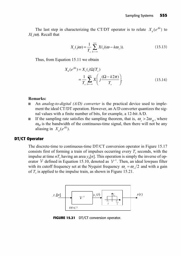
The last step in characterizing the CT/DT operator is to relate toX( j ). Recall that
(15.13)
Thus, from Equation 15.11 we obtain
(15.14)
Remarks:An analog-to-digital (A/D) converter is the practical device used to imple-ment the ideal CT/DT operation. However, an A/D converter quantizes the sig-nal values with a finite number of bits, for example, a 12-bit A/D.If the sampling rate satisfies the sampling theorem, that is, , where
M is the bandwidth of the continuous-time signal, then there will not be anyaliasing in .
DT/CT Operator
The discrete-time to continuous-time DT/CT conversion operator in Figure 15.17consists first of forming a train of impulses occurring every Ts seconds, with theimpulse at time nTs having an area yd[n]. This operation is simply the inverse of op-erator defined in Equation 15.10, denoted as . Then, an ideal lowpass filterwith its cutoff frequency set at the Nyquist frequency and with a gainof Ts is applied to the impulse train, as shown in Figure 15.21.
c s= 2V 1V
X ed
j( )
s M> 2
X e X j T
TX j
k
T
dj
s s
s sk
( ) ( )
( )
=
==
+1 2.
X jT
X j kss
sk
( ) ( ( )).==
+1
X ed
j( )
Sampling Systems 555
FIGURE 15.21 DT/CT conversion operator.
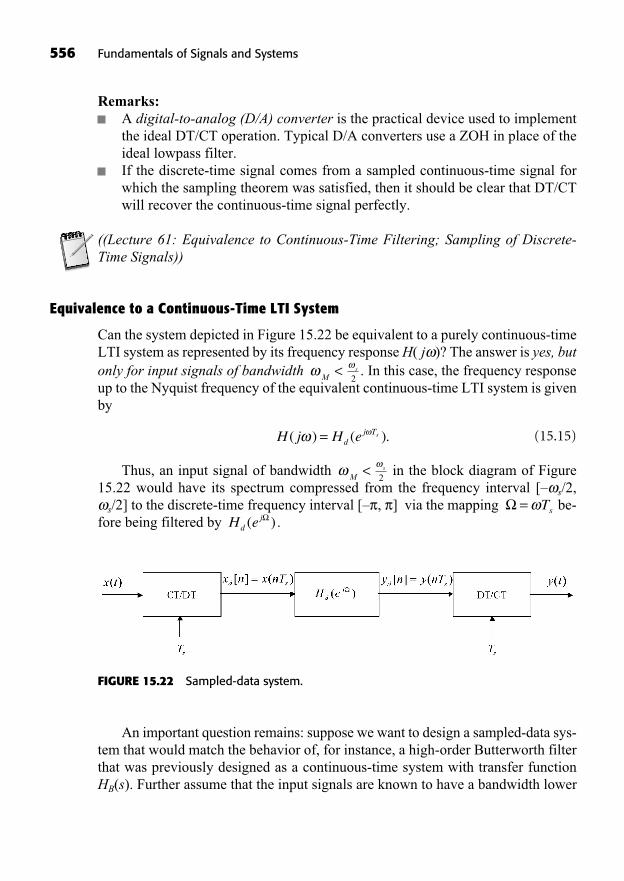
Remarks:A digital-to-analog (D/A) converter is the practical device used to implementthe ideal DT/CT operation. Typical D/A converters use a ZOH in place of theideal lowpass filter.If the discrete-time signal comes from a sampled continuous-time signal forwhich the sampling theorem was satisfied, then it should be clear that DT/CTwill recover the continuous-time signal perfectly.
((Lecture 61: Equivalence to Continuous-Time Filtering; Sampling of Discrete-Time Signals))
Equivalence to a Continuous-Time LTI System
Can the system depicted in Figure 15.22 be equivalent to a purely continuous-timeLTI system as represented by its frequency response H( j )? The answer is yes, butonly for input signals of bandwidth . In this case, the frequency responseup to the Nyquist frequency of the equivalent continuous-time LTI system is givenby
(15.15)
Thus, an input signal of bandwidth in the block diagram of Figure15.22 would have its spectrum compressed from the frequency interval [– s/2,
s/2] to the discrete-time frequency interval [– , ] via the mapping be-fore being filtered by .H ed
j( )= Ts
s
2M<
H j H edj Ts( ) ( ).=
s
2M<
556 Fundamentals of Signals and Systems
FIGURE 15.22 Sampled-data system.
An important question remains: suppose we want to design a sampled-data sys-tem that would match the behavior of, for instance, a high-order Butterworth filterthat was previously designed as a continuous-time system with transfer functionHB(s). Further assume that the input signals are known to have a bandwidth lower
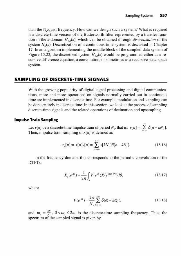
than the Nyquist frequency. How can we design such a system? What is requiredis a discrete-time version of the Butterworth filter represented by a transfer func-tion in the z-domain HBd(z), which can be obtained through discretization of thesystem HB(s). Discretization of a continuous-time system is discussed in Chapter17. In an algorithm implementing the middle block of the sampled-data system ofFigure 15.22, the discretized system HBd(z) would be programmed either as a re-cursive difference equation, a convolution, or sometimes as a recursive state-spacesystem.
SAMPLING OF DISCRETE-TIME SIGNALS
With the growing popularity of digital signal processing and digital communica-tions, more and more operations on signals normally carried out in continuoustime are implemented in discrete time. For example, modulation and sampling canbe done entirely in discrete time. In this section, we look at the process of samplingdiscrete-time signals and the related operations of decimation and upsampling.
Impulse Train Sampling
Let v[n] be a discrete-time impulse train of period Ns; that is, .Then, impulse train sampling of x[n] is defined as
(15.16)
In the frequency domain, this corresponds to the periodic convolution of theDTFTs:
(15.17)
where
(15.18)
and , is the discrete-time sampling frequency. Thus, thespectrum of the sampled signal is given by
s, <0 2sN
2s :=
V eN
kj
ss
k
( ) ( ),==
+2
X e V e X e dsj j j( ) ( ) ( ) ,( )=
1
2 2
x n x n v n x kN n kNs s sk
[ ] : [ ] [ ] [ ] [ ].= ==
+
n kNs[ ]k=
+
v n[ ] =
Sampling Systems 557
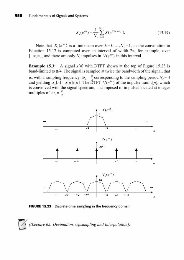
558 Fundamentals of Signals and Systems
(15.19)
Note that is a finite sum over , as the convolution inEquation 15.17 is computed over an interval of width 2 , for example, over
, and there are only Ns impulses in in this interval.
Example 15.3: A signal x[n] with DTFT shown at the top of Figure 15.23 isband-limited to /4. The signal is sampled at twice the bandwidth of the signal, that
is, with a sampling frequency corresponding to the sampling period Ns = 4and yielding . The DTFT of the impulse train v[n], whichis convolved with the signal spectrum, is composed of impulses located at integermultiples of .=
2s =
V ej( )x n x n v ns[ ] [ ] [ ]=2s =
V ej( )[ , ]
k Ns= 0 1, ,…X esj( )
X eN
X esj
s
j k
k
N
s
s
( ) ( ).( )==
1
0
1
FIGURE 15.23 Discrete-time sampling in the frequency domain.
((Lecture 62: Decimation, Upsampling and Interpolation))
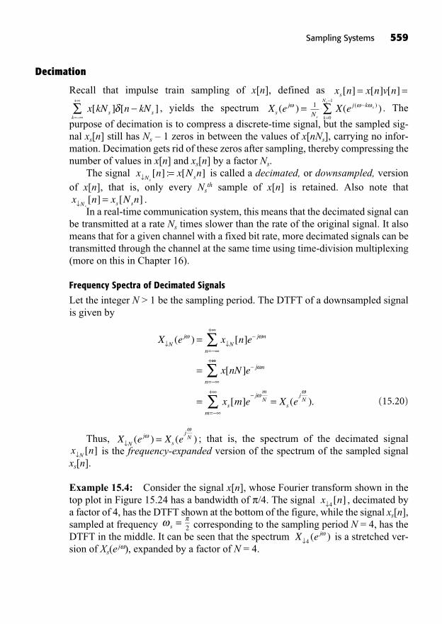
Decimation
Recall that impulse train sampling of x[n], defined as
, yields the spectrum . The
purpose of decimation is to compress a discrete-time signal, but the sampled sig-nal xs[n] still has Ns – 1 zeros in between the values of x[nNs], carrying no infor-mation. Decimation gets rid of these zeros after sampling, thereby compressing thenumber of values in x[n] and xs[n] by a factor Ns.
The signal is called a decimated, or downsampled, versionof x[n], that is, only every Ns
th sample of x[n] is retained. Also note that.
In a real-time communication system, this means that the decimated signal canbe transmitted at a rate Ns times slower than the rate of the original signal. It alsomeans that for a given channel with a fixed bit rate, more decimated signals can betransmitted through the channel at the same time using time-division multiplexing(more on this in Chapter 16).
Frequency Spectra of Decimated Signals
Let the integer N > 1 be the sampling period. The DTFT of a downsampled signalis given by
(15.20)
Thus, ; that is, the spectrum of the decimated signalis the frequency-expanded version of the spectrum of the sampled signal
xs[n].
Example 15.4: Consider the signal x[n], whose Fourier transform shown in thetop plot in Figure 15.24 has a bandwidth of /4. The signal , decimated bya factor of 4, has the DTFT shown at the bottom of the figure, while the signal xs[n],sampled at frequency corresponding to the sampling period N = 4, has theDTFT in the middle. It can be seen that the spectrum is a stretched ver-sion of Xs(e j ), expanded by a factor of N = 4.
X ej4( )
2s =
x n4[ ]
x nN
[ ]X e X e
Nj
s
jN=( ) ( )
X e x n e
x nN e
Nj
Nj n
n
j n
n
=
+
=
+
=
=
( ) [ ]
[ ]
=
+
= =x m e X es
jm
N
ms
jN[ ] ( ).
x n x N nN s ss
=[ ] [ ]
x n x N nN ss
=[ ] : [ ]
X ej k s( )( )
k
Ns
=0
1
Ns
1X esj( ) =x kN n kNs s[ ] [ ]
k=
+
x n x n v ns[ ] [ ] [ ]= =
Sampling Systems 559
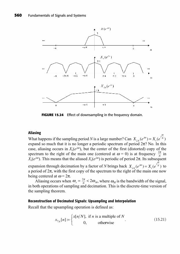
560 Fundamentals of Signals and Systems
Aliasing
What happens if the sampling period N is a large number? Can expand so much that it is no longer a periodic spectrum of period 2 ? No. In thiscase, aliasing occurs in Xs(e j ), but the center of the first (distorted) copy of thespectrum to the right of the main one (centered at = 0) is at frequency inXs(e j ). This means that the aliased Xs(e j ) is periodic of period 2 . Its subsequent
expansion through decimation by a factor of N brings back toa period of 2 , with the first copy of the spectrum to the right of the main one nowbeing centered at = 2 .
Aliasing occurs when , where M is the bandwidth of the signal,in both operations of sampling and decimation. This is the discrete-time version ofthe sampling theorem.
Reconstruction of Decimated Signals: Upsampling and Interpolation
Recall that the upsampling operation is defined as:
(15.21)x nx n N n N
N=[ ] :
[ ],
,
if is a multiple of
othe0 rrwise.
M< 2N
2s =
X e X eN
js
jN=( ) ( )
2
N
X e X eN
js
jN=( ) ( )
FIGURE 15.24 Effect of downsampling in the frequency domain.
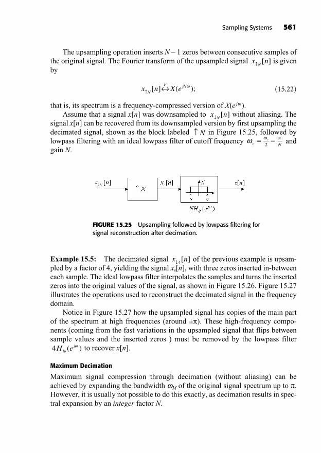
The upsampling operation inserts N – 1 zeros between consecutive samples ofthe original signal. The Fourier transform of the upsampled signal is givenby
(15.22)
that is, its spectrum is a frequency-compressed version of X(e j ).Assume that a signal x[n] was downsampled to without aliasing. The
signal x[n] can be recovered from its downsampled version by first upsampling thedecimated signal, shown as the block labeled in Figure 15.25, followed bylowpass filtering with an ideal lowpass filter of cutoff frequency = andgain N.
Ns
2c =N
x nN
[ ]
x n X eN
F jN[ ] ( );
x nN
[ ]
Sampling Systems 561
FIGURE 15.25 Upsampling followed by lowpass filtering forsignal reconstruction after decimation.
Example 15.5: The decimated signal of the previous example is upsam-pled by a factor of 4, yielding the signal xs[n], with three zeros inserted in-betweeneach sample. The ideal lowpass filter interpolates the samples and turns the insertedzeros into the original values of the signal, as shown in Figure 15.26. Figure 15.27illustrates the operations used to reconstruct the decimated signal in the frequencydomain.
Notice in Figure 15.27 how the upsampled signal has copies of the main partof the spectrum at high frequencies (around ± ). These high-frequency compo-nents (coming from the fast variations in the upsampled signal that flips betweensample values and the inserted zeros ) must be removed by the lowpass filter
to recover x[n].
Maximum Decimation
Maximum signal compression through decimation (without aliasing) can beachieved by expanding the bandwidth M of the original signal spectrum up to .However, it is usually not possible to do this exactly, as decimation results in spec-tral expansion by an integer factor N.
4H elpj( )
x n4[ ]
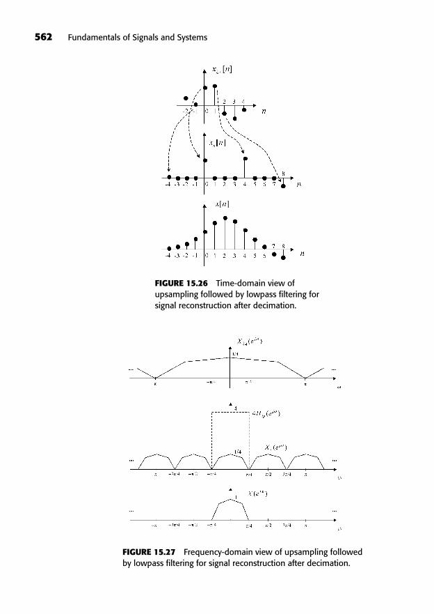
562 Fundamentals of Signals and Systems
FIGURE 15.26 Time-domain view ofupsampling followed by lowpass filtering forsignal reconstruction after decimation.
FIGURE 15.27 Frequency-domain view of upsampling followedby lowpass filtering for signal reconstruction after decimation.
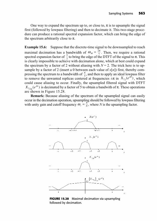
One way to expand the spectrum up to, or close to, is to upsample the signalfirst (followed by lowpass filtering) and then to decimate it. This two-stage proce-dure can produce a rational spectral expansion factor, which can bring the edge ofthe spectrum arbitrarily close to .
Example 15.6: Suppose that the discrete-time signal to be downsampled to reach
maximal decimation has a bandwidth of . Then, we require a rationalspectral expansion factor of to bring the edge of the DTFT of the signal to . Thisis clearly impossible to achieve with decimation alone, which at best could expandthe spectrum by a factor of 2 without aliasing with N = 2. The trick here is to up-sample by a factor of 2 (insert a 0 between each value of x[n]) first, thereby com-pressing the spectrum to a bandwidth of , and then to apply an ideal lowpass filterto remove the unwanted replicas centered at frequencies ± in , whichcould cause aliasing to occur. Finally, the upsampled filtered signal with DTFT
is decimated by a factor of 5 to obtain a bandwith of . These operationsare shown in Figure 15.28.
Remark: Because aliasing of the spectrum of the upsampled signal can easilyoccur in the decimation operation, upsampling should be followed by lowpass filteringwith unity gain and cutoff frequency , where N is the upsampling factor.Nc =
X elp
j2
( )
X ej2( )
5
5
2
=2
5M =
Sampling Systems 563
FIGURE 15.28 Maximal decimation via upsamplingfollowed by decimation.
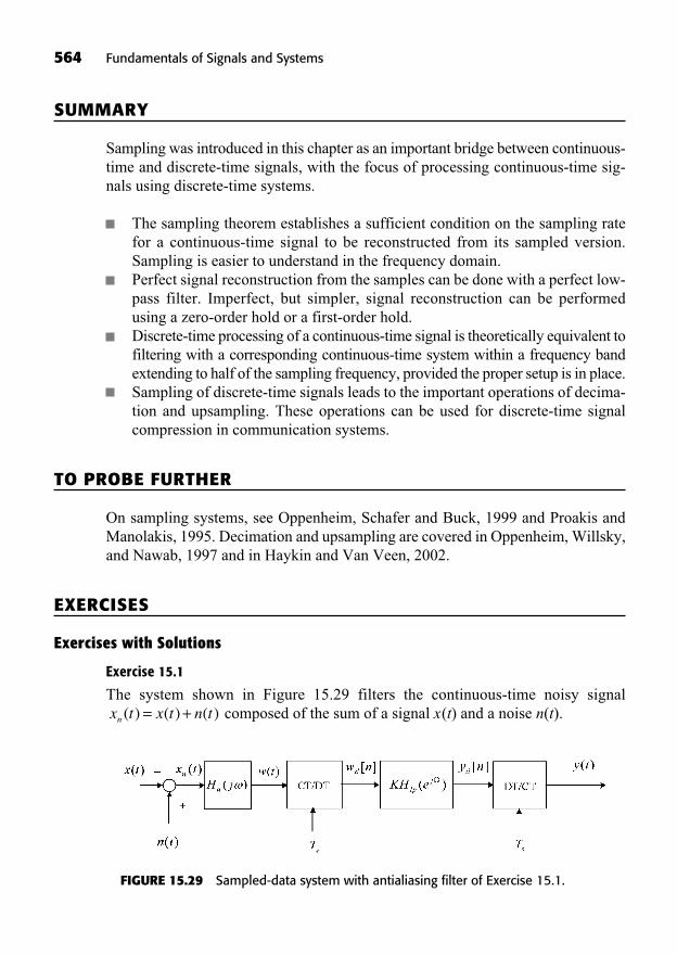
SUMMARY
Sampling was introduced in this chapter as an important bridge between continuous-time and discrete-time signals, with the focus of processing continuous-time sig-nals using discrete-time systems.
The sampling theorem establishes a sufficient condition on the sampling ratefor a continuous-time signal to be reconstructed from its sampled version.Sampling is easier to understand in the frequency domain.Perfect signal reconstruction from the samples can be done with a perfect low-pass filter. Imperfect, but simpler, signal reconstruction can be performedusing a zero-order hold or a first-order hold.Discrete-time processing of a continuous-time signal is theoretically equivalent tofiltering with a corresponding continuous-time system within a frequency bandextending to half of the sampling frequency, provided the proper setup is in place.Sampling of discrete-time signals leads to the important operations of decima-tion and upsampling. These operations can be used for discrete-time signalcompression in communication systems.
TO PROBE FURTHER
On sampling systems, see Oppenheim, Schafer and Buck, 1999 and Proakis andManolakis, 1995. Decimation and upsampling are covered in Oppenheim, Willsky,and Nawab, 1997 and in Haykin and Van Veen, 2002.
EXERCISES
Exercises with Solutions
Exercise 15.1
The system shown in Figure 15.29 filters the continuous-time noisy signalcomposed of the sum of a signal x(t) and a noise n(t).x t x t n tn ( ) ( ) ( )= +
564 Fundamentals of Signals and Systems
FIGURE 15.29 Sampled-data system with antialiasing filter of Exercise 15.1.

Sampling Systems 565
The signal and noise have their respective spectrum, X( j ), N( j ) shown inFigure 15.30. The frequency response of the antialiasing lowpass filter is alsoshown in the figure.
FIGURE 15.30 Antialiasing filter and signal and noise spectra inExercise 15.1.
(a) Let the sampling frequency be rad/s. Sketch the spectrumW( j ) of the signal w(t). Also sketch the spectrum . Indicate theimportant frequencies and magnitudes on your sketch. Discuss the results.
Answer:The Nyquist frequency is . The spectra W( j ) and are shownin Figure 15.31.
W edj( )5500=s
2
W edj( )
s = 11000
FIGURE 15.31 Fourier transform of output of antialiasing filterand DTFT of signal after CT/DT (Exercise 15.1).
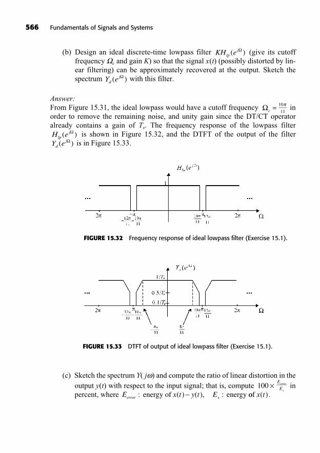
566 Fundamentals of Signals and Systems
(b) Design an ideal discrete-time lowpass filter (give its cutofffrequency c and gain K) so that the signal x(t) (possibly distorted by lin-ear filtering) can be approximately recovered at the output. Sketch thespectrum with this filter.
Answer:From Figure 15.31, the ideal lowpass would have a cutoff frequency inorder to remove the remaining noise, and unity gain since the DT/CT operatoralready contains a gain of Ts. The frequency response of the lowpass filter
is shown in Figure 15.32, and the DTFT of the output of the filteris in Figure 15.33.Y ed
j( )H elp
j( )
10
11c =
Y edj( )
KH elpj( )
FIGURE 15.32 Frequency response of ideal lowpass filter (Exercise 15.1).
FIGURE 15.33 DTFT of output of ideal lowpass filter (Exercise 15.1).
(c) Sketch the spectrum Y( j ) and compute the ratio of linear distortion in theoutput y(t) with respect to the input signal; that is, compute inpercent, where .E x t y t Eerror x: ( ) ( ), : energy of energy oof x t( )
E
Eerror
x100 ×
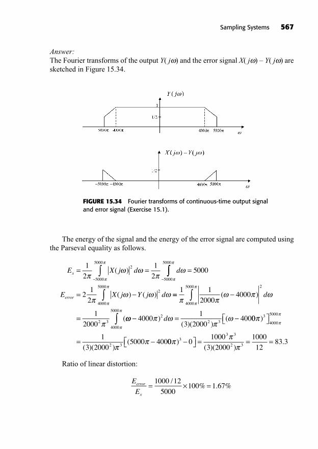
Answer:The Fourier transforms of the output Y( j ) and the error signal X( j ) – Y( j ) aresketched in Figure 15.34.
Sampling Systems 567
FIGURE 15.34 Fourier transforms of continuous-time output signaland error signal (Exercise 15.1).
The energy of the signal and the energy of the error signal are computed usingthe Parseval equality as follows.
Ratio of linear distortion:
E
Eerror
x
= × =1000 12
5000100 1 67
/% . %
E X j d dx = =1
2
1
22
5000
5000
5000
5000
( ) =
=
5000
21
22
4000
5000
E X j Y j derror ( ) ( ) ==
=
1 1
20004000
1
2000
2
4000
5000
2 3
( )
(
d
=40001
3 20004002
4000
5000
2 3)( )( )
(d 00
1
3 20005000 400
3
4000
5000
2 3
)
( )( )(= 00 0
1000
3 2000
1000
1283 33
3 3
2 3)( )( )
.= = =
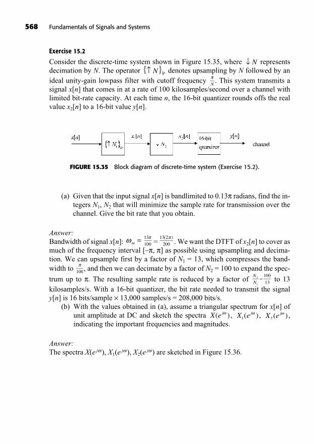
568 Fundamentals of Signals and Systems
Exercise 15.2
Consider the discrete-time system shown in Figure 15.35, where representsdecimation by N. The operator denotes upsampling by N followed by anideal unity-gain lowpass filter with cutoff frequency . This system transmits asignal x[n] that comes in at a rate of 100 kilosamples/second over a channel withlimited bit-rate capacity. At each time n, the 16-bit quantizer rounds offs the realvalue x2[n] to a 16-bit value y[n].
N
{ }N lp
N
FIGURE 15.35 Block diagram of discrete-time system (Exercise 15.2).
(a) Given that the input signal x[n] is bandlimited to 0.13 radians, find the in-tegers N1, N2 that will minimize the sample rate for transmission over thechannel. Give the bit rate that you obtain.
Answer:Bandwidth of signal x[n]: = . We want the DTFT of x2[n] to cover asmuch of the frequency interval [– , ] as possible using upsampling and decima-tion. We can upsample first by a factor of N1 = 13, which compresses the band-width to , and then we can decimate by a factor of N2 = 100 to expand the spec-
trum up to . The resulting sample rate is reduced by a factor of to 13 kilosamples/s. With a 16-bit quantizer, the bit rate needed to transmit the signaly[n] is 16 bits/sample × 13,000 samples/s = 208,000 bits/s.
(b) With the values obtained in (a), assume a triangular spectrum for x[n] ofunit amplitude at DC and sketch the spectra , , , indicating the important frequencies and magnitudes.
Answer:The spectra X(e j ), X1(e j ), X2(e j ) are sketched in Figure 15.36.
X ej2 ( )X ej1( )X ej( )
N
N2
1
100
13=
100
13 2
200
( )13
100m =
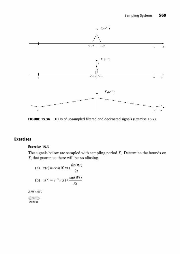
Exercises
Exercise 15.3
The signals below are sampled with sampling period Ts. Determine the bounds onTs that guarantee there will be no aliasing.
(a)
(b)
Answer:
x t e u tWt
tt( ) ( )
sin( )= 4
x t tt
t( ) cos( )
sin( )= 10
2
Sampling Systems 569
FIGURE 15.36 DTFTs of upsampled filtered and decimated signals (Exercise 15.2).
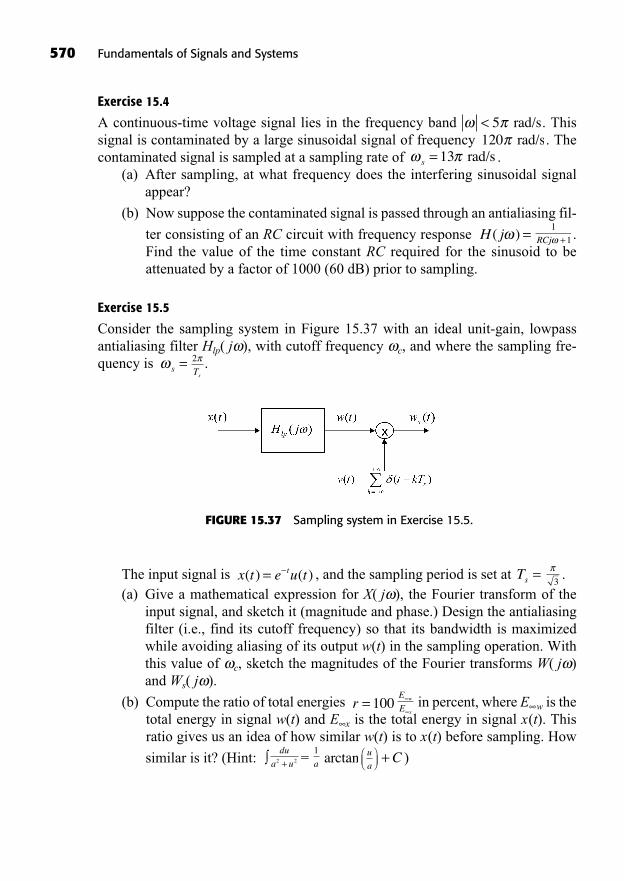
570 Fundamentals of Signals and Systems
Exercise 15.4
A continuous-time voltage signal lies in the frequency band . Thissignal is contaminated by a large sinusoidal signal of frequency . Thecontaminated signal is sampled at a sampling rate of .
(a) After sampling, at what frequency does the interfering sinusoidal signalappear?
(b) Now suppose the contaminated signal is passed through an antialiasing fil-
ter consisting of an RC circuit with frequency response .Find the value of the time constant RC required for the sinusoid to beattenuated by a factor of 1000 (60 dB) prior to sampling.
Exercise 15.5
Consider the sampling system in Figure 15.37 with an ideal unit-gain, lowpassantialiasing filter Hlp( j ), with cutoff frequency c, and where the sampling fre-quency is .
sT
2s =
RCj +1
1H j( ) =
s = 13 rad/s120 rad/s< 5 rad/s
FIGURE 15.37 Sampling system in Exercise 15.5.
The input signal is , and the sampling period is set at .(a) Give a mathematical expression for X( j ), the Fourier transform of the
input signal, and sketch it (magnitude and phase.) Design the antialiasingfilter (i.e., find its cutoff frequency) so that its bandwidth is maximizedwhile avoiding aliasing of its output w(t) in the sampling operation. Withthis value of c, sketch the magnitudes of the Fourier transforms W( j )and Ws( j ).
(b) Compute the ratio of total energies in percent, where E w is thetotal energy in signal w(t) and E x is the total energy in signal x(t). Thisratio gives us an idea of how similar w(t) is to x(t) before sampling. How
similar is it? (Hint: = )C+u
aarctana
1du
a u2 2+
E
Ew
xr = 100
3Ts =x t e u tt( ) ( )=

Answer:
Exercise 15.6
Consider the sampling system in Figure 15.38, where the sampling frequency is.
sT
2s =
Sampling Systems 571
FIGURE 15.38 Sampling system in Exercise 15.6.
The input signal is and the spectra of the ideal bandpassfilter and the ideal lowpass filter are shown in Figure 15.39.
Wt
2sinc2W=
2
2x t( ) =
FIGURE 15.39 Frequency responses of ideal lowpass and bandpass filters inExercise 15.6.
(a) Compute and sketch X( j ), the Fourier transform of the input signal. Forwhat range of sampling frequencies is the sampling theorem sat-isfied for the first sampler?
(b) Assume that the sampling theorem is satisfied with the slowest samplingfrequency s in the range found in (a). Sketch the spectra Y( j ), W( j ),and Z( j ) for this case.
sT
2s =
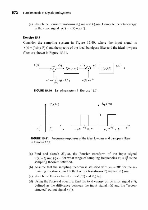
572 Fundamentals of Signals and Systems
(c) Sketch the Fourier transforms Xr( j ) and E( j ). Compute the total energyin the error signal .
Exercise 15.7
Consider the sampling system in Figure 15.40, where the input signal is
and the spectra of the ideal bandpass filter and the ideal lowpass
filter are shown in Figure 15.41.
x t tW W( ) )= sinc (
e t x t x tr
( ) : ( ) ( )=
FIGURE 15.40 Sampling system in Exercise 15.7.
FIGURE 15.41 Frequency responses of the ideal lowpass and bandpass filtersin Exercise 15.7.
(a) Find and sketch X( j ), the Fourier transform of the input signal. For what range of sampling frequencies is the
sampling theorem satisfied?
(b) Assume that the sampling theorem is satisfied with for the re-maining questions. Sketch the Fourier transforms Y( j ) and W( j ).
(c) Sketch the Fourier transforms Z( j ) and Xr( j ).
(d) Using the Parseval equality, find the total energy of the error signal e(t), defined as the difference between the input signal x(t) and the “recon-structed” output signal xr(t).
s W= 3
sT
2s =x t tW W( ) )= sinc (
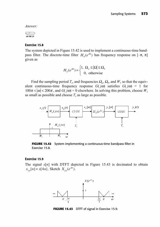
Answer:
Exercise 15.8
The system depicted in Figure 15.42 is used to implement a continuous-time band-pass filter. The discrete-time filter has frequency response on [– , ]given as
Find the sampling period Ts, and frequencies a, b, and W1 so that the equiv-alent continuous-time frequency response G( j ) satisfies G( j ) = 1 for
, and G( j ) = 0 elsewhere. In solving this problem, choose W1
as small as possible and choose Ts as large as possible.100 200< <
H edj a b( )
,
,=
1
0 otherwise
H edj( )
Sampling Systems 573
FIGURE 15.42 System implementing a continuous-time bandpass filter inExercise 15.8.
Exercise 15.9
The signal x[n] with DTFT depicted in Figure 15.43 is decimated to obtain. Sketch .X ej
4( )x n x n=
44[ ] [ ]
FIGURE 15.43 DTFT of signal in Exercise 15.9.
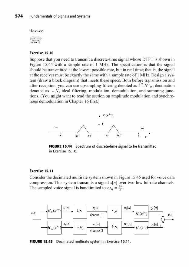
574 Fundamentals of Signals and Systems
Answer:
Exercise 15.10
Suppose that you need to transmit a discrete-time signal whose DTFT is shown inFigure 15.44 with a sample rate of 1 MHz. The specification is that the signalshould be transmitted at the lowest possible rate, but in real time; that is, the signalat the receiver must be exactly the same with a sample rate of 1 MHz. Design a sys-tem (draw a block diagram) that meets these specs. Both before transmission andafter reception, you can use upsampling-filtering denoted as , decimationdenoted as , ideal filtering, modulation, demodulation, and summing junc-tions. (You might want to read the section on amplitude modulation and synchro-nous demodulation in Chapter 16 first.)
N{ }N lp
FIGURE 15.44 Spectrum of discrete-time signal to be transmittedin Exercise 15.10.
Exercise 15.11
Consider the decimated multirate system shown in Figure 15.45 used for voice datacompression. This system transmits a signal x[n] over two low-bit-rate channels.The sampled voice signal is bandlimited to .2
5M =
FIGURE 15.45 Decimated multirate system in Exercise 15.11.

Numerical values:Input lowpass filter’s cutoff frequency
Input highpass filter’s cutoff frequency
Signal’s spectrum over [– , ]:
(a) Sketch the spectra X(e j ), X1(e j ), and X2(e j ), indicating the importantfrequencies and magnitudes.
(b) Find the maximum decimation factors N1 and N2, avoiding aliasing, andsketch the corresponding spectra V1(e j ), V2(e j ), W1(e j ), and W2(e j ), in-dicating the important frequencies and magnitudes. Specify what the idealoutput filters H1(e j ) and H2(e j ) should be for perfect signal reconstruc-tion. Sketch their frequency responses, indicating the important frequen-cies and magnitudes.
(c) Compute the ratio of total energies at the output between the high-frequency subband y2[n] and the output signal x[n]; that is, compute
, where the energy is given by .
(d) Now suppose each of the two signal subbands v1[n] and v2[n] are quantizedwith a different number of bits to achieve good data compression, withoutlosing intelligibility of the voice message. According to your result in (c), it would seem to make sense to use fewer bits to quantize the high-frequency subband. Suppose that the filter bank operates at an input/outputsample rate of 10 kHz, and you decide to use 12 bits to quantize v1[n] and4 bits to quantize v2[n]. Compute the bit rates of channel 1 and channel 2and the overall bit rate of the system.
Answer:
y n[ ]2
n=
+
E y =:%E
Ey
y
2r := 100
,
, < <
15
2
2
5
02
5
X ej( ) =
3chp =3clp =
Sampling Systems 575

This page intentionally left blank
577
Introduction toCommunication Systems
16
In This Chapter
Complex Exponential and Sinusoidal Amplitude ModulationDemodulation of Sinusoidal AMSingle-Sideband Amplitude ModulationModulation of a Pulse-Train CarrierPulse-Amplitude ModulationTime-Division MultiplexingFrequency-Division MultiplexingAngle ModulationSummaryTo Probe FurtherExercises
((Lecture 63: Amplitude Modulation and Synchronous Demodulation))
The field of telecommunications engineering has radically changed our livesby allowing us to communicate with other people from virtually any loca-tion on earth and even from space. Who could have imagined two hundred
years ago that this could ever be possible? The study of communication systems islargely based on signals and systems theory. In particular, the time-domain multi-plication property of Fourier transforms is used in amplitude modulation. Thischapter is a brief introduction to the basic theory of modulation for signal trans-mission.

578 Fundamentals of Signals and Systems
COMPLEX EXPONENTIAL AND SINUSOIDAL AMPLITUDE MODULATION
Recall the time-domain multiplication property for Fourier transforms: the multi-plication of two signals results in the convolution of their spectra:
(16.1)
Amplitude modulation (AM) is based on this property. For example, considerthe modulation system described by
(16.2)
where the modulated signal y(t) is the product of the carrier signal c(t) and themodulating signal x(t), also called the message. The carrier signal can be a complexexponential or a sinusoid, or even a pulse train.
An important objective in modulation is to produce a signal whose frequencyrange is suitable for transmission over the communication channel to be used. Intelephone systems, long-distance transmission is often accomplished over mi-crowave (300 MHz to 300 GHz) or satellite links (300 MHz to 40 GHz), but mostof the energy of a voice signal is in the range of 50 Hz to 5 kHz. Hence, voice sig-nals have to be shifted to much higher frequencies for efficient transmission. Thiscan be achieved by amplitude modulation.
Amplitude Modulation with a Complex Exponential Carrier
In amplitude modulation with a complex exponential carrier, the latter can be writ-ten as
(16.3)
where the frequency c is called the carrier frequency. Let c = 0 for convenience.We have seen that the Fourier transform of a complex exponential is an impulse ofarea 2 , so that
(16.4)
The frequency-domain convolution of C( j ) and X( j ) yields
C jc
( ) ( ).= 2
c t e j tc c( ) ,( )= +
y t x t c t( ) ( ) ( ),=
x t y t X j Y jFT
( ) ( ) ( ) ( ).1
2
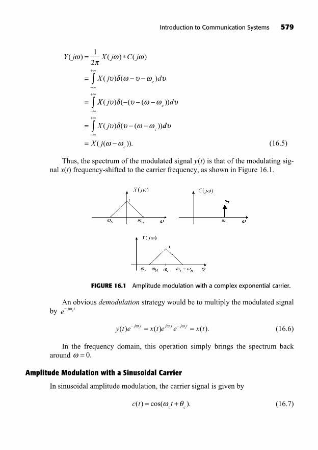
(16.5)
Thus, the spectrum of the modulated signal y(t) is that of the modulating sig-nal x(t) frequency-shifted to the carrier frequency, as shown in Figure 16.1.
An obvious demodulation strategy would be to multiply the modulated signalby
(16.6)
In the frequency domain, this operation simply brings the spectrum backaround
Amplitude Modulation with a Sinusoidal Carrier
In sinusoidal amplitude modulation, the carrier signal is given by
(16.7)c t tc c
( ) cos( ).= +
= 0.
y t e x t e e x tj t j t j tc c c( ) ( ) ( ).= =
e j tc
Y j X j C j
X j dc
( ) ( ) ( )
( ) ( )
=
=
=
+
1
2
XX j d
X j
c
c
( ) ( ( ( ))
( ) ( ( ))=
+
dd
X jc
+
= ( ( )).
Introduction to Communication Systems 579
FIGURE 16.1 Amplitude modulation with a complex exponential carrier.
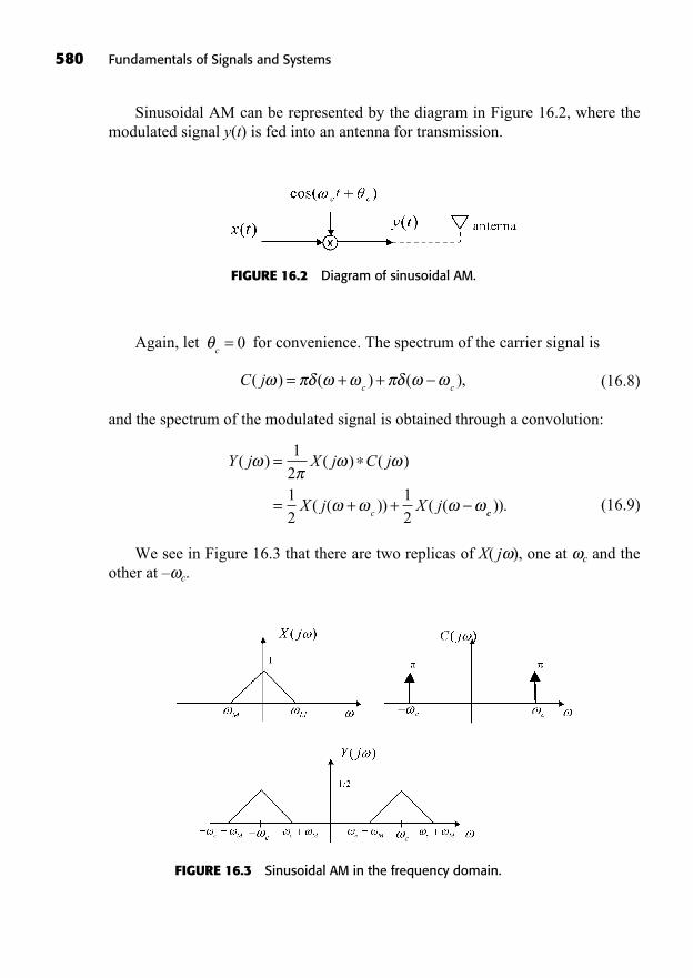
580 Fundamentals of Signals and Systems
Sinusoidal AM can be represented by the diagram in Figure 16.2, where themodulated signal y(t) is fed into an antenna for transmission.
FIGURE 16.2 Diagram of sinusoidal AM.
FIGURE 16.3 Sinusoidal AM in the frequency domain.
Again, let for convenience. The spectrum of the carrier signal is
(16.8)
and the spectrum of the modulated signal is obtained through a convolution:
(16.9)
We see in Figure 16.3 that there are two replicas of X( j ), one at c and theother at – c.
Y j X j C j
X j X jc
( ) ( ) ( )
( ( )) ( (
=
= + +
1
21
2
1
2 cc)).
C jc c
( ) ( ) ( ),= + +
c= 0
Note that the two copies of the original spectrum can overlap if the carrier fre-quency is not high enough, that is, if c < M, which is not the case for AM with acomplex exponential carrier. The modulating signal may be unrecoverable if thishappens.
DEMODULATION OF SINUSOIDAL AM
In a communication system, the information-bearing (modulating) signal x(t) is re-covered at the receiver end through demodulation. There are two commonly usedmethods for sinusoidal AM demodulation: synchronous demodulation, in whichthe transmitter and receiver are synchronized and in phase, and asynchronousdemodulation, which does not require accurate knowledge of the carrier signal.
Synchronous Demodulation
Assuming that c > M, synchronous demodulation is straightforward. Considerthe modulated signal to be demodulated:
(16.10)
If we multiply this signal again by the carrier at the receiver, that is,
(16.11)
then the two replicas of Y( j ) will be such that the left part of one adds up to theright part of the other, thereby reforming the original spectrum of x(t) around
= 0. Then x(t) can be recovered by an ideal lowpass filter with a gain of 2 andcutoff frequency co, satisfying This principle of synchro-nous demodulation is illustrated by Figure 16.4.
Also, using the trigonometric identity,
(16.12)
we can express the signal (t) as follows:
(16.13)
w t x t t
x t x t t
c
c
( ) ( )cos ( )
( ) ( )cos( ),
=
= +
2
1
2
1
22
cos ( ) cos( ),2 1
2
1
22
c ct t= +
M co c M< < 2 .
w t y t tc
( ) ( )cos( ),=
cos( )ct
y t x t tc
( ) ( )cos( ).=
Introduction to Communication Systems 581
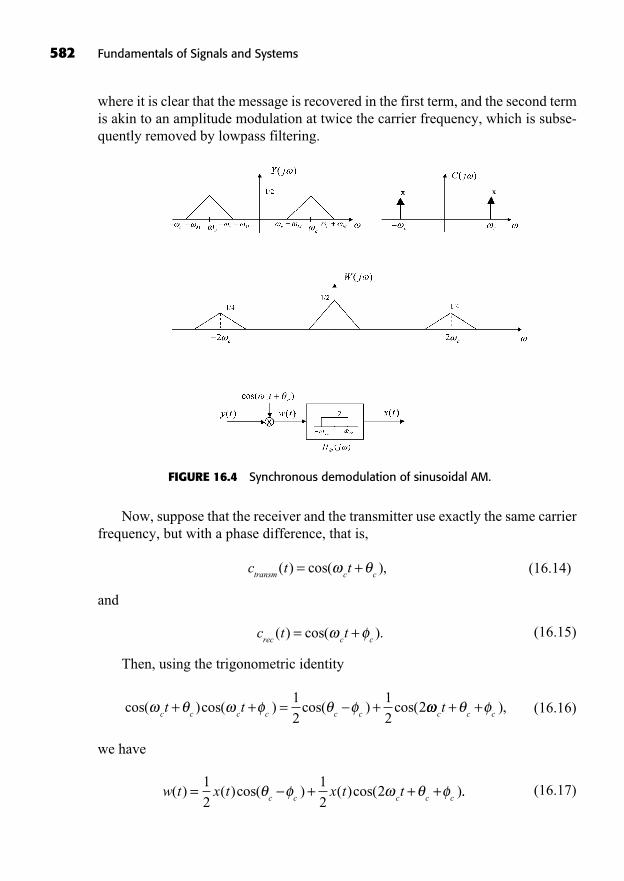
582 Fundamentals of Signals and Systems
where it is clear that the message is recovered in the first term, and the second termis akin to an amplitude modulation at twice the carrier frequency, which is subse-quently removed by lowpass filtering.
Now, suppose that the receiver and the transmitter use exactly the same carrierfrequency, but with a phase difference, that is,
(16.14)
and
(16.15)
Then, using the trigonometric identity
(16.16)
we have
(16.17)w t x t x t tc c c c c
( ) ( )cos( ) ( )cos( )= + + +1
2
1
22 ..
cos( )cos( ) cos( ) cos(c c c c c ct t+ + = +
1
2
1
22
c c ct + + ),
c t trec c c
( ) cos( ).= +
c t ttransm c c
( ) cos( ),= +
FIGURE 16.4 Synchronous demodulation of sinusoidal AM.

This means that the amplitude of the signal recovered at the output of thelowpass filter is smaller than the original amplitude by a factor of Inparticular, when the demodulating carrier is out of phase by the output of thedemodulator is zero.
Equation 16.17 also helps explain the beating phenomenon heard on someolder radio receivers in which the volume of a demodulated voice or music signalseems to periodically go up and down. Suppose that the phase of the receiver’scarrier is actually the linear function of time where is a very small realnumber in proportion to the carrier frequency. In this case, the carrier frequencyused by the receiver is slightly off with respect to the carrier frequency used tomodulate the signal as
(16.18)
Then, Equation 16.17 becomes
(16.19)
where the amplitude of the first term containing the message is affected by a sinu-soidal gain which produces the beating effect.
((Lecture 64: Asynchronous Demodulation))
Asynchronous Demodulation
In contrast to synchronous demodulation of AM signals, asynchronous demodula-tion does not require that the receiver have very accurate knowledge of the carrier’sphase and frequency. Asynchronous demodulation is used in simple AM radio re-ceivers: it is a cheap, but lower quality, alternative to synchronous demodulation.
Asynchronous demodulation involves a nonlinear operation and is thereforeeasier to understand in the time domain. Suppose that we add a positive constant tothe signal to be transmitted before modulation:
(16.20)
where A is large enough to make This amounts to transmitting thecarrier signal as well as the modulated signal. Let K be the maximum amplitude ofx(t), that is, and assume A ≥ K. The modulation index m is the ratio
(16.21)m K A: .=
x t K( ) ,<
A x t t+ >( ) , .0
y t A x t tc( ) ( ) cos( ),= +
cos( ),tc
+
w t x t t x t tc c c c
( ) ( )cos( ) ( )cos( )= + + + +1
2
1
22 ,,
c t t t trec c c c
( ) cos( ( )) cos(( ) ).= + = +
ct= ,
2,cos( ).
c c
Introduction to Communication Systems 583
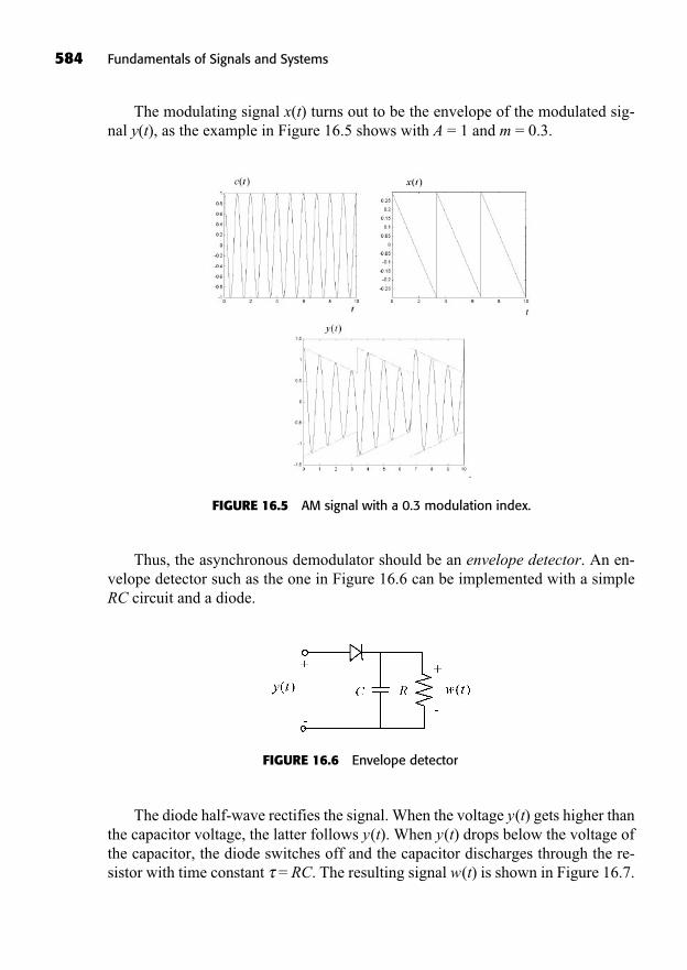
The modulating signal x(t) turns out to be the envelope of the modulated sig-nal y(t), as the example in Figure 16.5 shows with A = 1 and m = 0.3.
584 Fundamentals of Signals and Systems
FIGURE 16.5 AM signal with a 0.3 modulation index.
FIGURE 16.6 Envelope detector
Thus, the asynchronous demodulator should be an envelope detector. An en-velope detector such as the one in Figure 16.6 can be implemented with a simpleRC circuit and a diode.
The diode half-wave rectifies the signal. When the voltage y(t) gets higher thanthe capacitor voltage, the latter follows y(t). When y(t) drops below the voltage ofthe capacitor, the diode switches off and the capacitor discharges through the re-sistor with time constant = RC. The resulting signal w(t) is shown in Figure 16.7.
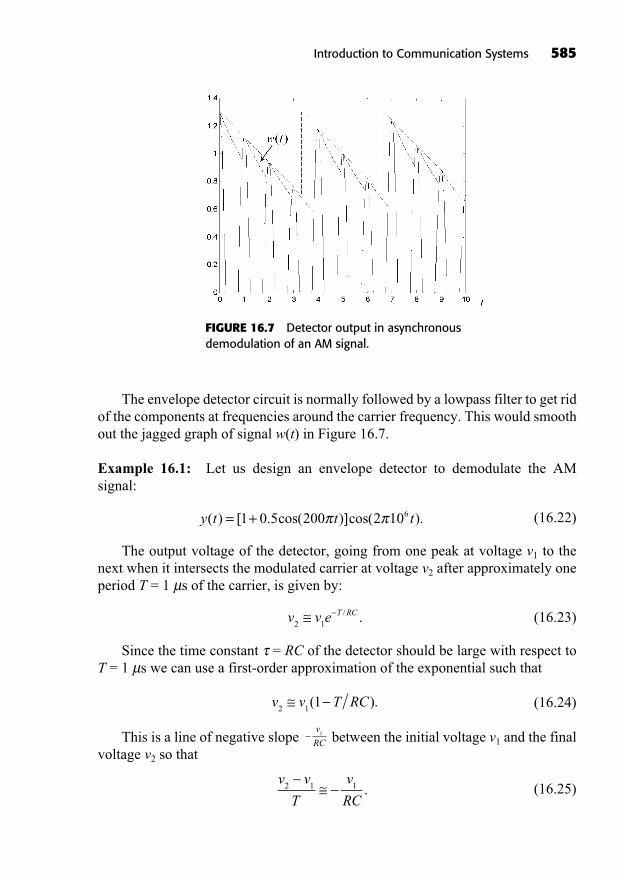
The envelope detector circuit is normally followed by a lowpass filter to get ridof the components at frequencies around the carrier frequency. This would smoothout the jagged graph of signal w(t) in Figure 16.7.
Example 16.1: Let us design an envelope detector to demodulate the AM signal:
(16.22)
The output voltage of the detector, going from one peak at voltage v1 to thenext when it intersects the modulated carrier at voltage v2 after approximately oneperiod T = 1 μs of the carrier, is given by:
(16.23)
Since the time constant = RC of the detector should be large with respect toT = 1 μs we can use a first-order approximation of the exponential such that
(16.24)
This is a line of negative slope between the initial voltage v1 and the finalvoltage v2 so that
(16.25)v v
T
v
RC2 1 1 .
v
RC1
v v T RC2 1
1( ).
v v e T RC2 1
/ .
y t t t( ) [ . cos( )]cos( ).= +1 0 5 200 2 106
Introduction to Communication Systems 585
FIGURE 16.7 Detector output in asynchronousdemodulation of an AM signal.
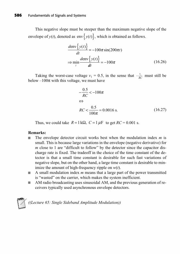
586 Fundamentals of Signals and Systems
This negative slope must be steeper than the maximum negative slope of the
envelope of y(t), denoted as which is obtained as follows.
(16.26)
Taking the worst-case voltage v1 = 0.5, in the sense that must still bebelow –100 with this voltage, we must have
(16.27)
Thus, we could take to get RC = 0.001 s.
Remarks:The envelope detector circuit works best when the modulation index m issmall. This is because large variations in the envelope (negative derivative) form close to 1 are “difficult to follow” by the detector since the capacitor dis-charge rate is fixed. The tradeoff in the choice of the time constant of the de-tector is that a small time constant is desirable for such fast variations ofnegative slope, but on the other hand, a large time constant is desirable to min-imize the amount of high-frequency ripple on w(t).A small modulation index m means that a large part of the power transmittedis “wasted” on the carrier, which makes the system inefficient.AM radio broadcasting uses sinusoidal AM, and the previous generation of re-ceivers typically used asynchronous envelope detectors.
((Lecture 65: Single Sideband Amplitude Modulation))
R C= =1 1k F, μ
<
< =
0 5100
0 5
1000 0016
.
..
RC
RC s.
v
RC1
d y t
dtt
d y t
t
env
env
( )sin( )
min( )
{ }=
{ }100 200
ddt= 100
env y t( ) ,{ }
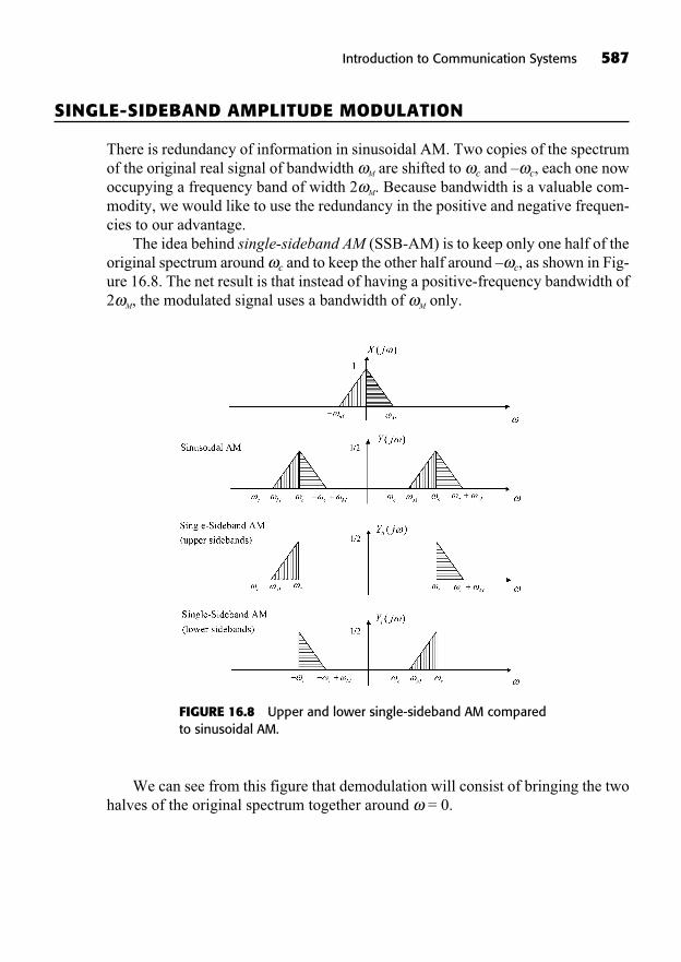
SINGLE-SIDEBAND AMPLITUDE MODULATION
There is redundancy of information in sinusoidal AM. Two copies of the spectrumof the original real signal of bandwidth M are shifted to c and – c, each one nowoccupying a frequency band of width 2 M. Because bandwidth is a valuable com-modity, we would like to use the redundancy in the positive and negative frequen-cies to our advantage.
The idea behind single-sideband AM (SSB-AM) is to keep only one half of theoriginal spectrum around c and to keep the other half around – c, as shown in Fig-ure 16.8. The net result is that instead of having a positive-frequency bandwidth of2 M, the modulated signal uses a bandwidth of M only.
Introduction to Communication Systems 587
FIGURE 16.8 Upper and lower single-sideband AM comparedto sinusoidal AM.
We can see from this figure that demodulation will consist of bringing the twohalves of the original spectrum together around = 0.
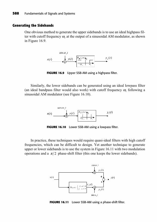
Generating the Sidebands
One obvious method to generate the upper sidebands is to use an ideal highpass fil-ter with cutoff frequency c at the output of a sinusoidal AM modulator, as shownin Figure 16.9.
588 Fundamentals of Signals and Systems
FIGURE 16.9 Upper SSB-AM using a highpass filter.
FIGURE 16.10 Lower SSB-AM using a lowpass filter.
FIGURE 16.11 Lower SSB-AM using a phase-shift filter.
Similarly, the lower sidebands can be generated using an ideal lowpass filter(an ideal bandpass filter would also work) with cutoff frequency c following asinusoidal AM modulator (see Figure 16.10).
In practice, these techniques would require quasi-ideal filters with high cutofffrequencies, which can be difficult to design. Yet another technique to generateupper or lower sidebands is to use the system in Figure 16.11 with two modulationoperations and a phase-shift filter (this one keeps the lower sidebands).2
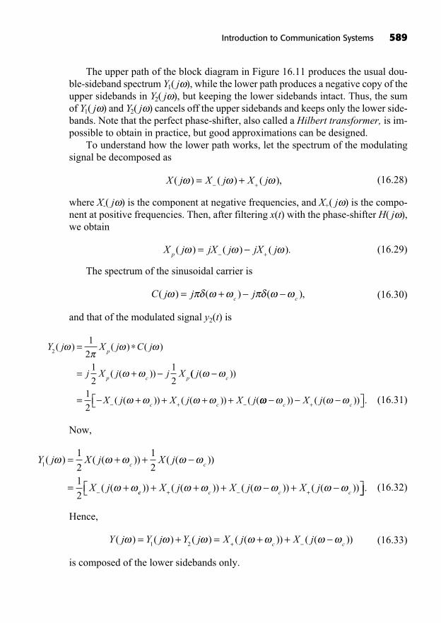
The upper path of the block diagram in Figure 16.11 produces the usual dou-ble-sideband spectrum Y1( j ), while the lower path produces a negative copy of theupper sidebands in Y2( j ), but keeping the lower sidebands intact. Thus, the sumof Y1( j ) and Y2( j ) cancels off the upper sidebands and keeps only the lower side-bands. Note that the perfect phase-shifter, also called a Hilbert transformer, is im-possible to obtain in practice, but good approximations can be designed.
To understand how the lower path works, let the spectrum of the modulatingsignal be decomposed as
(16.28)
where X-( j ) is the component at negative frequencies, and X+( j ) is the compo-nent at positive frequencies. Then, after filtering x(t) with the phase-shifter H( j ),we obtain
(16.29)
The spectrum of the sinusoidal carrier is
(16.30)
and that of the modulated signal y2(t) is
(16.31)
Now,
(16.32)
Hence,
(16.33)
is composed of the lower sidebands only.
Y j Y j Y j X j X jc c
( ) ( ) ( ) ( ( )) ( ( ))= + = + ++1 2
Y j X j X j
X j
c c1
1
2
1
21
2
( ) ( ( )) ( ( ))
( (
= + +
= +cc c c c
X j X j X j)) ( ( )) ( ( )) ( ( ))+ + + ++ + .
Y j X j C j
j X j j X
p
p c p
2
1
21
2
1
2
( ) ( ) ( )
( ( ))
=
= + (( ( ))
( ( )) ( ( )) ( (
j
X j X j X j
c
c c= + + + ++
1
2 +c cX j)) ( ( )) .
C j j jc c
( ) ( ) ( ),= +
X j jX j jX jp( ) ( ) ( ).= +
X j X j X j( ) ( ) ( ),= + +
Introduction to Communication Systems 589
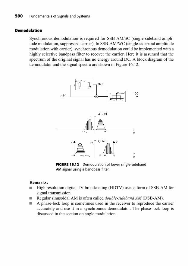
Demodulation
Synchronous demodulation is required for SSB-AM/SC (single-sideband ampli-tude modulation, suppressed carrier). In SSB-AM/WC (single-sideband amplitudemodulation with carrier), synchronous demodulation could be implemented with ahighly selective bandpass filter to recover the carrier. Here it is assumed that thespectrum of the original signal has no energy around DC. A block diagram of thedemodulator and the signal spectra are shown in Figure 16.12.
590 Fundamentals of Signals and Systems
FIGURE 16.12 Demodulation of lower single-sidebandAM signal using a bandpass filter.
Remarks:High resolution digital TV broadcasting (HDTV) uses a form of SSB-AM forsignal transmission.Regular sinusoidal AM is often called double-sideband AM (DSB-AM).A phase-lock loop is sometimes used in the receiver to reproduce the carrieraccurately and use it in a synchronous demodulator. The phase-lock loop isdiscussed in the section on angle modulation.
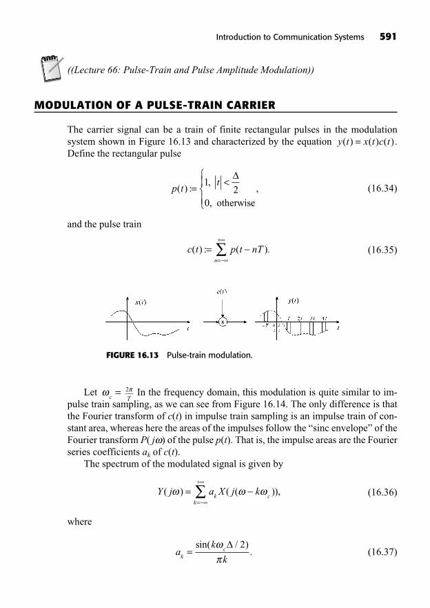
((Lecture 66: Pulse-Train and Pulse Amplitude Modulation))
MODULATION OF A PULSE-TRAIN CARRIER
The carrier signal can be a train of finite rectangular pulses in the modulation system shown in Figure 16.13 and characterized by the equation .Define the rectangular pulse
(16.34)
and the pulse train
(16.35)c t p t nTn
( ) : ( ).==
+
p tt
( ) :,
,
,= <12
0 otherwise
y t x t c t( ) ( ) ( )=
Introduction to Communication Systems 591
FIGURE 16.13 Pulse-train modulation.
Let In the frequency domain, this modulation is quite similar to im-pulse train sampling, as we can see from Figure 16.14. The only difference is thatthe Fourier transform of c(t) in impulse train sampling is an impulse train of con-stant area, whereas here the areas of the impulses follow the “sinc envelope” of theFourier transform P( j ) of the pulse p(t). That is, the impulse areas are the Fourierseries coefficients ak of c(t).
The spectrum of the modulated signal is given by
(16.36)
where
(16.37)ak
kkc=
sin( / ).
2
Y j a X j kk c
k
( ) ( ( )),==
+
T
2c=
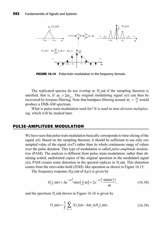
592 Fundamentals of Signals and Systems
The replicated spectra do not overlap in Y( j ) if the sampling theorem is satisfied, that is, if The original modulating signal x(t) can then berecovered by lowpass filtering. Note that bandpass filtering around wouldproduce a DSB-AM spectrum.
What is pulse-train modulation used for? It is used in time-division multiplex-ing, which will be studied later.
PULSE-AMPLITUDE MODULATION
We have seen that pulse-train modulation basically corresponds to time-slicing of thesignal x(t). Based on the sampling theorem, it should be sufficient to use only onesampled value of the signal x(nT) rather than its whole continuous range of valuesover the pulse duration. This type of modulation is called pulse-amplitude modula-tion (PAM). The analysis is different from pulse-;train modulation: rather than ob-taining scaled, undistorted copies of the original spectrum in the modulated signaly(t), PAM creates some distortion in the spectral replicas in Y( j ). This distortioncomes from the zero-order-hold (ZOH)–like operation as shown in Figure 16.15.
The frequency response H0( j ) of h0(t) is given by
(16.38)
and the spectrum Y( j ) shown in Figure 16.16 is given by
(16.39)Y jT
X j k H jc
k
( ) ( ( )) ( ).==
+10
H j e ej j
02 2 22( )
sin( ),= ( ) =sinc 2
T
2c=
c M> 2 .
FIGURE 16.14 Pulse-train modulation in the frequency domain.
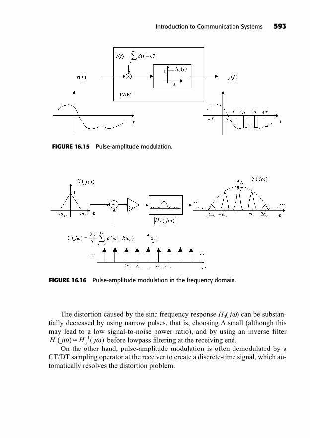
The distortion caused by the sinc frequency response H0( j ) can be substan-tially decreased by using narrow pulses, that is, choosing small (although thismay lead to a low signal-to-noise power ratio), and by using an inverse filter
before lowpass filtering at the receiving end.On the other hand, pulse-amplitude modulation is often demodulated by a
CT/DT sampling operator at the receiver to create a discrete-time signal, which au-tomatically resolves the distortion problem.
H j H j1 0
1( ) ( )
Introduction to Communication Systems 593
FIGURE 16.15 Pulse-amplitude modulation.
FIGURE 16.16 Pulse-amplitude modulation in the frequency domain.
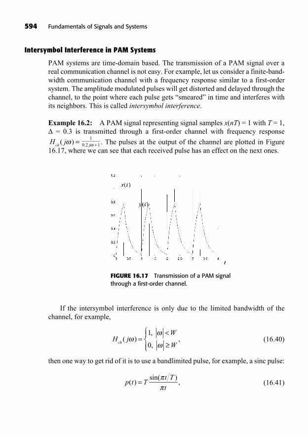
594 Fundamentals of Signals and Systems
Intersymbol Interference in PAM Systems
PAM systems are time-domain based. The transmission of a PAM signal over areal communication channel is not easy. For example, let us consider a finite-band-width communication channel with a frequency response similar to a first-ordersystem. The amplitude modulated pulses will get distorted and delayed through thechannel, to the point where each pulse gets “smeared” in time and interferes withits neighbors. This is called intersymbol interference.
Example 16.2: A PAM signal representing signal samples x(nT) = 1 with T = 1,= 0.3 is transmitted through a first-order channel with frequency response
. The pulses at the output of the channel are plotted in Figure16.17, where we can see that each received pulse has an effect on the next ones.
j. +1
0 2 1H jch
( ) =
FIGURE 16.17 Transmission of a PAM signalthrough a first-order channel.
If the intersymbol interference is only due to the limited bandwidth of thechannel, for example,
(16.40)
then one way to get rid of it is to use a bandlimited pulse, for example, a sinc pulse:
(16.41)p t Tt T
t( )
sin( ),=
H jW
Wch( )
,
,,=
<1
0
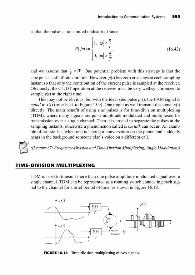
so that the pulse is transmitted undistorted since
(16.42)
and we assume that One potential problem with this strategy is that the
sinc pulse is of infinite duration. However, p(t) has zero crossings at each samplinginstant so that only the contribution of the current pulse is sampled at the receiver.Obviously, the CT/DT operation at the receiver must be very well synchronized tosample y(t) at the right time.
This may not be obvious, but with the ideal sinc pulse p(t), the PAM signal isequal to x(t) (refer back to Figure 15.9). One might as well transmit the signal x(t)directly. The main benefit of using sinc pulses is for time-division multiplexing(TDM), where many signals are pulse-amplitude modulated and multiplexed fortransmission over a single channel. Then it is crucial to separate the pulses at thesampling instants; otherwise a phenomenon called crosstalk can occur. An exam-ple of crosstalk is when one is having a conversation on the phone and suddenlyhears in the background someone else’s voice on a different call.
((Lecture 67: Frequency-Division and Time-Division Multiplexing; Angle Modulation))
TIME-DIVISION MULTIPLEXING
TDM is used to transmit more than one pulse-amplitude modulated signal over asingle channel. TDM can be represented as a rotating switch connecting each sig-nal to the channel for a brief period of time, as shown in Figure 16.18.
W< .T
P j T
T
( ),
,
,=<
>
1
0
Introduction to Communication Systems 595
FIGURE 16.18 Time-division multiplexing of two signals.
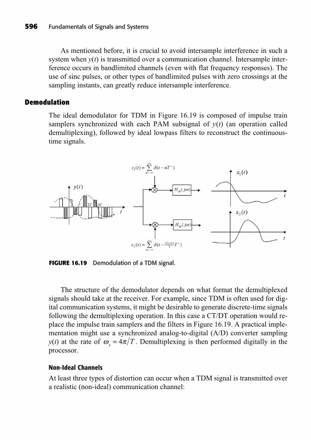
596 Fundamentals of Signals and Systems
As mentioned before, it is crucial to avoid intersample interference in such asystem when y(t) is transmitted over a communication channel. Intersample inter-ference occurs in bandlimited channels (even with flat frequency responses). Theuse of sinc pulses, or other types of bandlimited pulses with zero crossings at thesampling instants, can greatly reduce intersample interference.
Demodulation
The ideal demodulator for TDM in Figure 16.19 is composed of impulse trainsamplers synchronized with each PAM subsignal of y(t) (an operation called demultiplexing), followed by ideal lowpass filters to reconstruct the continuous-time signals.
FIGURE 16.19 Demodulation of a TDM signal.
The structure of the demodulator depends on what format the demultiplexedsignals should take at the receiver. For example, since TDM is often used for dig-ital communication systems, it might be desirable to generate discrete-time signalsfollowing the demultiplexing operation. In this case a CT/DT operation would re-place the impulse train samplers and the filters in Figure 16.19. A practical imple-mentation might use a synchronized analog-to-digital (A/D) converter samplingy(t) at the rate of . Demultiplexing is then performed digitally in theprocessor.
Non-Ideal Channels
At least three types of distortion can occur when a TDM signal is transmitted overa realistic (non-ideal) communication channel:
s T= 4
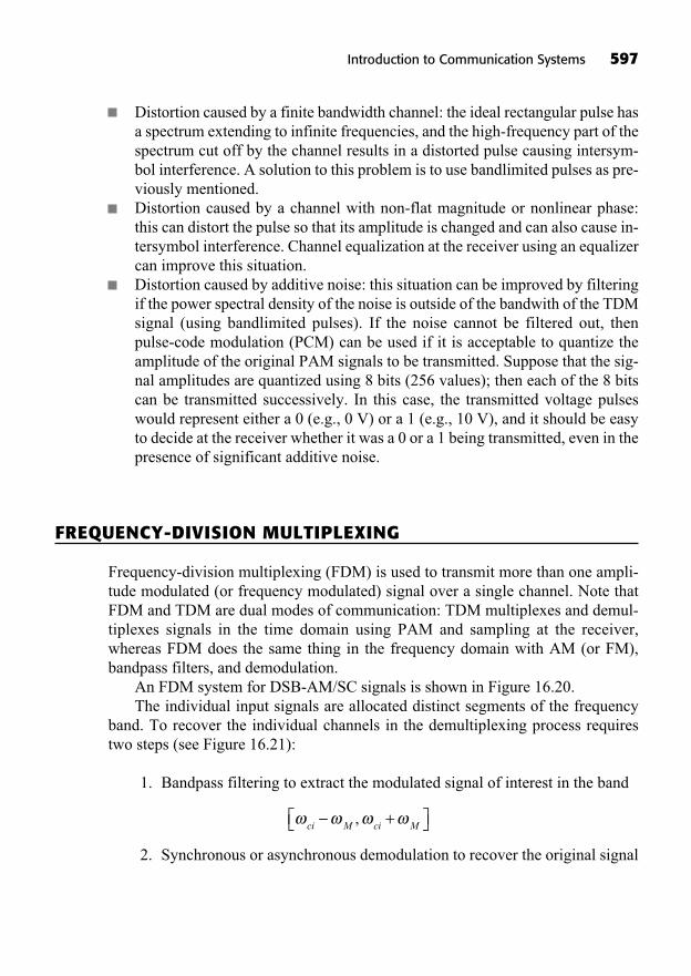
Distortion caused by a finite bandwidth channel: the ideal rectangular pulse hasa spectrum extending to infinite frequencies, and the high-frequency part of thespectrum cut off by the channel results in a distorted pulse causing intersym-bol interference. A solution to this problem is to use bandlimited pulses as pre-viously mentioned.Distortion caused by a channel with non-flat magnitude or nonlinear phase:this can distort the pulse so that its amplitude is changed and can also cause in-tersymbol interference. Channel equalization at the receiver using an equalizercan improve this situation.Distortion caused by additive noise: this situation can be improved by filteringif the power spectral density of the noise is outside of the bandwith of the TDMsignal (using bandlimited pulses). If the noise cannot be filtered out, thenpulse-code modulation (PCM) can be used if it is acceptable to quantize theamplitude of the original PAM signals to be transmitted. Suppose that the sig-nal amplitudes are quantized using 8 bits (256 values); then each of the 8 bitscan be transmitted successively. In this case, the transmitted voltage pulseswould represent either a 0 (e.g., 0 V) or a 1 (e.g., 10 V), and it should be easyto decide at the receiver whether it was a 0 or a 1 being transmitted, even in thepresence of significant additive noise.
FREQUENCY-DIVISION MULTIPLEXING
Frequency-division multiplexing (FDM) is used to transmit more than one ampli-tude modulated (or frequency modulated) signal over a single channel. Note thatFDM and TDM are dual modes of communication: TDM multiplexes and demul-tiplexes signals in the time domain using PAM and sampling at the receiver,whereas FDM does the same thing in the frequency domain with AM (or FM),bandpass filters, and demodulation.
An FDM system for DSB-AM/SC signals is shown in Figure 16.20.The individual input signals are allocated distinct segments of the frequency
band. To recover the individual channels in the demultiplexing process requirestwo steps (see Figure 16.21):
1. Bandpass filtering to extract the modulated signal of interest in the band
2. Synchronous or asynchronous demodulation to recover the original signal
ci M ci M+,
Introduction to Communication Systems 597
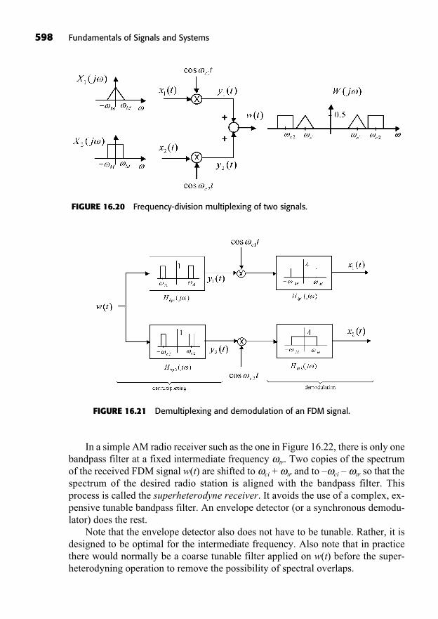
598 Fundamentals of Signals and Systems
In a simple AM radio receiver such as the one in Figure 16.22, there is only onebandpass filter at a fixed intermediate frequency IF. Two copies of the spectrumof the received FDM signal w(t) are shifted to ci + IF and to – ci – IF so that thespectrum of the desired radio station is aligned with the bandpass filter. Thisprocess is called the superheterodyne receiver. It avoids the use of a complex, ex-pensive tunable bandpass filter. An envelope detector (or a synchronous demodu-lator) does the rest.
Note that the envelope detector also does not have to be tunable. Rather, it isdesigned to be optimal for the intermediate frequency. Also note that in practicethere would normally be a coarse tunable filter applied on w(t) before the super-heterodyning operation to remove the possibility of spectral overlaps.
FIGURE 16.20 Frequency-division multiplexing of two signals.
FIGURE 16.21 Demultiplexing and demodulation of an FDM signal.
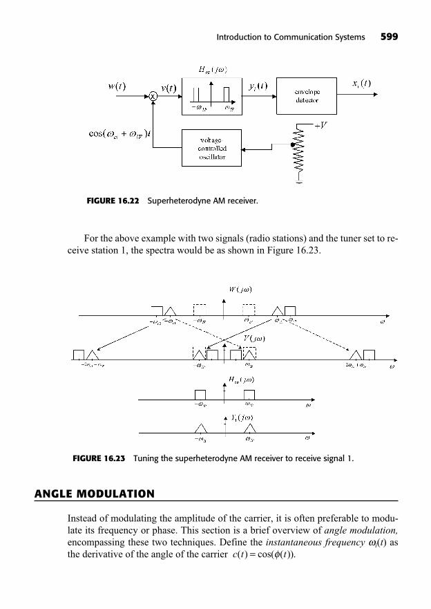
For the above example with two signals (radio stations) and the tuner set to re-ceive station 1, the spectra would be as shown in Figure 16.23.
Introduction to Communication Systems 599
FIGURE 16.22 Superheterodyne AM receiver.
FIGURE 16.23 Tuning the superheterodyne AM receiver to receive signal 1.
ANGLE MODULATION
Instead of modulating the amplitude of the carrier, it is often preferable to modu-late its frequency or phase. This section is a brief overview of angle modulation,encompassing these two techniques. Define the instantaneous frequency i(t) asthe derivative of the angle of the carrier c t t( ) cos( ( )).=

(16.43)
The integral form is
(16.44)
In amplitude modulation, we have and Note that anglemodulation is difficult to analyze in the frequency domain, so this is outside of thescope of this book.
Frequency Modulation
In frequency modulation, the instantaneous modulation frequency is set to
(16.45)
so that
(16.46)
and the frequency modulated signal is given by
(16.47)
Note that its amplitude is constant.
Phase Modulation
In phase modulation, the angle is set to
(16.48)
and the phase modulated signal is given by
(16.49)y t A t k x tc f( ) cos ( ) .= +( )
( ) ( ),t t k xc f= +
y t A t k x dc f
t
( ) cos ( ) .= +
( ) ( ) ,t t k x dc f
t
= +
i c ft k x t( ) ( ),= +
i ct( ) .=( )t tc=
( ) ( ) .t di
t
=
i tddt
t( ) : ( )=
600 Fundamentals of Signals and Systems
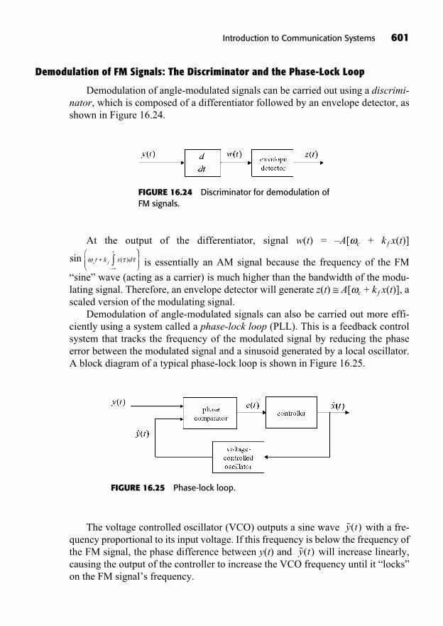
Demodulation of FM Signals: The Discriminator and the Phase-Lock Loop
Demodulation of angle-modulated signals can be carried out using a discrimi-nator, which is composed of a differentiator followed by an envelope detector, asshown in Figure 16.24.
Introduction to Communication Systems 601
FIGURE 16.24 Discriminator for demodulation ofFM signals.
At the output of the differentiator, signal w(t) = –A[ c + k f x(t)]
is essentially an AM signal because the frequency of the FM
“sine” wave (acting as a carrier) is much higher than the bandwidth of the modu-lating signal. Therefore, an envelope detector will generate z(t) A[ c + k f x(t)], ascaled version of the modulating signal.
Demodulation of angle-modulated signals can also be carried out more effi-ciently using a system called a phase-lock loop (PLL). This is a feedback controlsystem that tracks the frequency of the modulated signal by reducing the phaseerror between the modulated signal and a sinusoid generated by a local oscillator.A block diagram of a typical phase-lock loop is shown in Figure 16.25.
t k x dc f
t
( )+sin
FIGURE 16.25 Phase-lock loop.
The voltage controlled oscillator (VCO) outputs a sine wave with a fre-quency proportional to its input voltage. If this frequency is below the frequency ofthe FM signal, the phase difference between y(t) and will increase linearly,causing the output of the controller to increase the VCO frequency until it “locks”on the FM signal’s frequency.
y t( )
y t( )
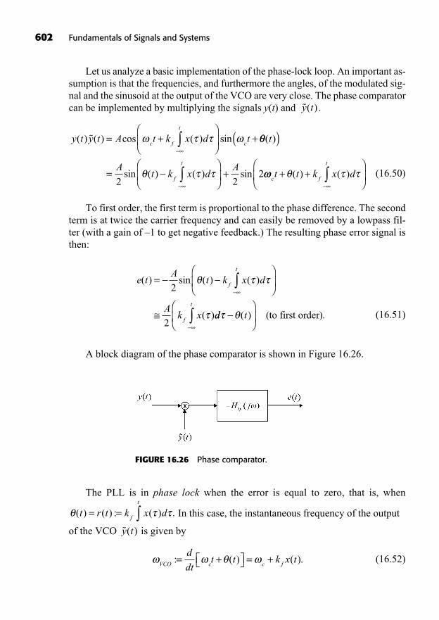
602 Fundamentals of Signals and Systems
Let us analyze a basic implementation of the phase-lock loop. An important as-sumption is that the frequencies, and furthermore the angles, of the modulated sig-nal and the sinusoid at the output of the VCO are very close. The phase comparatorcan be implemented by multiplying the signals y(t) and .
(16.50)
To first order, the first term is proportional to the phase difference. The secondterm is at twice the carrier frequency and can easily be removed by a lowpass fil-ter (with a gain of –1 to get negative feedback.) The resulting phase error signal isthen:
(16.51)
A block diagram of the phase comparator is shown in Figure 16.26.
e tA
t k x d
Ak x
f
t
f
( ) sin ( ) ( )
( )
=2
2dd t
t
( ) (to first order).
y t y t A t k x d tc f
t
c( ) ( ) cos ( ) sin = + + ( )
sin ( ) ( ) sin
t
At k x d
Af
t
( )
= +2 2
2c f
t
t t k x d+ +( ) ( )
y t( )
FIGURE 16.26 Phase comparator.
The PLL is in phase lock when the error is equal to zero, that is, when
In this case, the instantaneous frequency of the output
of the VCO is given by
(16.52)VCO c c f
d
dtt t k x t: ( ) ( ).= + = +
y t( )
( ) ( ) : ( ) .t r t k x df
t
= =
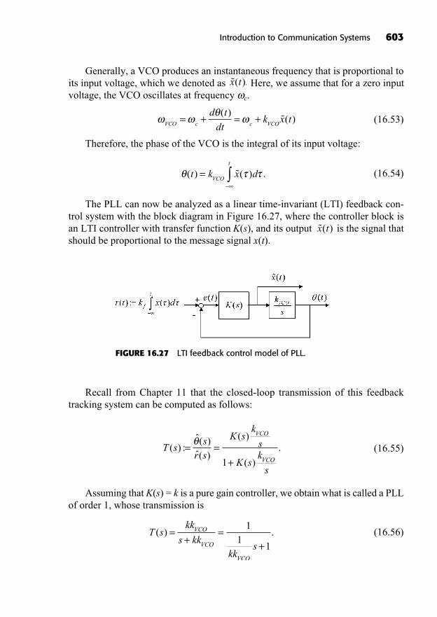
Generally, a VCO produces an instantaneous frequency that is proportional toits input voltage, which we denoted as Here, we assume that for a zero inputvoltage, the VCO oscillates at frequency c.
(16.53)
Therefore, the phase of the VCO is the integral of its input voltage:
(16.54)
The PLL can now be analyzed as a linear time-invariant (LTI) feedback con-trol system with the block diagram in Figure 16.27, where the controller block isan LTI controller with transfer function K(s), and its output is the signal thatshould be proportional to the message signal x(t).
x t( )
( ) ( ) .t k x dVCO
t
=
VCO c c VCO
d t
dtk x t= + = +
( )( )
x t( ).
Introduction to Communication Systems 603
FIGURE 16.27 LTI feedback control model of PLL.
Recall from Chapter 11 that the closed-loop transmission of this feedbacktracking system can be computed as follows:
(16.55)
Assuming that K(s) = k is a pure gain controller, we obtain what is called a PLLof order 1, whose transmission is
(16.56)T skk
s kkkk
s
VCO
VCO
VCO
( ) .=+
=+
11
1
T ss
r s
K sk
s
K sk
s
VCO
VCO
( ) :ˆ( )ˆ( )
( )
( )
.= =+1
604 Fundamentals of Signals and Systems
The DC gain of this closed-loop transfer function is 1, which represents near-perfect tracking of the phase of the FM signal when it changes slowly. The magni-tude of the Bode plot of T(s) stays close to 1 (0 dB) up until the break frequency
This frequency must be made higher than the bandwidth of the refer-ence signal, which is essentially the bandwidth of the message signal (modulo the
effect of integration), by selecting the controller gain k appropriately. Alsorecall that the linear approximation of the sine function of the phase error holds forsmall angles only. This is another important consideration to keep in mind in thedesign of K(s), as the PLL could “unlock” if the error becomes too large.
Finally, the message-bearing signal of interest in the PLL is the output of thecontroller, which is given by
(16.57)
Thus, signal is a filtered version of where the deriva-
tive comes from the numerator s, but the effect of the first-order lowpass filtercan be neglected if the controller gain k is chosen high enough, which
pushes the cutoff frequency outside of the bandwidth of the messagesignal. Therefore, with a large controller gain, the first-order PLL effectively de-modulates the FM signal by giving the voltage signal:
(16.58)
SUMMARY
This chapter was a brief introduction to the theory of communication systems.
Amplitude modulation of a message signal is obtained by multiplying the sig-nal with a sinusoidal carrier. This shifts the spectrum of the message and re-centers it around the carrier frequency. The AM signal can be demodulated bya synchronous demodulator whose frequency must be made equal to the carrierfrequency, or by a simpler asynchronous demodulator essentially consisting ofan envelope detector.
x tk
kx tf
VCO
( ) ( ).
11
1kk
sVCO
+
x t( ),k
kf
VCOr t( ) =d
dt x t( )
( ) ˆ( )x sk
kk
s
kss kk
r sk
s
kkVCO VCO VCO
VC
=+
=+
=1
11
OO
sr s
+1
ˆ( ).
1 j
0= kk
VCO.
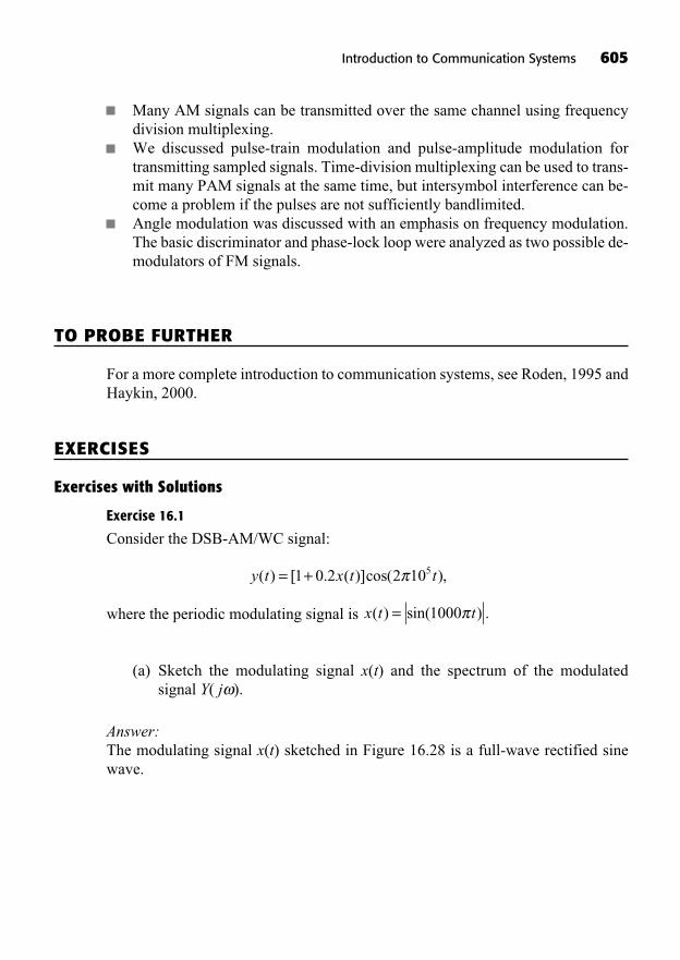
Many AM signals can be transmitted over the same channel using frequencydivision multiplexing.We discussed pulse-train modulation and pulse-amplitude modulation fortransmitting sampled signals. Time-division multiplexing can be used to trans-mit many PAM signals at the same time, but intersymbol interference can be-come a problem if the pulses are not sufficiently bandlimited.Angle modulation was discussed with an emphasis on frequency modulation.The basic discriminator and phase-lock loop were analyzed as two possible de-modulators of FM signals.
TO PROBE FURTHER
For a more complete introduction to communication systems, see Roden, 1995 andHaykin, 2000.
EXERCISES
Exercises with Solutions
Exercise 16.1
Consider the DSB-AM/WC signal:
where the periodic modulating signal is
(a) Sketch the modulating signal x(t) and the spectrum of the modulated signal Y( j ).
Answer:The modulating signal x(t) sketched in Figure 16.28 is a full-wave rectified sinewave.
x t t( ) sin( ) .= 1000
y t x t t( ) [ . ( )]cos( ),= +1 0 2 2 105
Introduction to Communication Systems 605
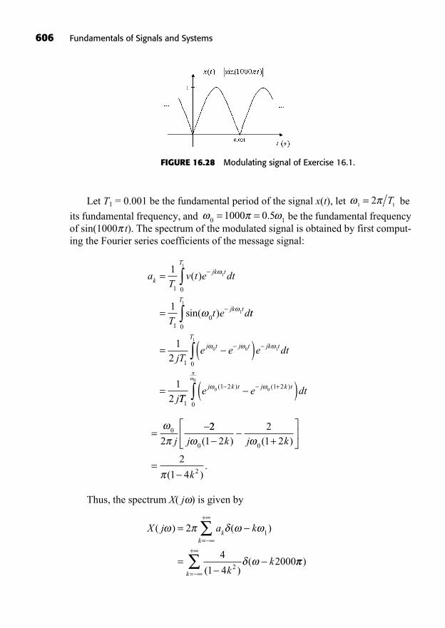
Let T1 = 0.001 be the fundamental period of the signal x(t), let be
its fundamental frequency, and be the fundamental frequencyof sin(1000 t). The spectrum of the modulated signal is obtained by first comput-ing the Fourier series coefficients of the message signal:
Thus, the spectrum X( j ) is given by
X j a k
kk
kk
( ) ( )
( )(
=
=
=
+
2
4
1 42000
1
2)
k=
+
j0
2= 22
1 221 2
2
1 4
0 0
2
j k j k
k
( ) ( )
( ).
+
=
aT
v t e dt
Tt e d
kjk t
T
jk t
=
=
1
1
1 0
10
1
1
1
( )
sin( ) tt
jTe e e dt
j
T
j t j t jk tT
0
1 0
1
0 0 1
112
12
= ( )
=TT
e e dtj k t j k t
1
1 2 1 2
0
0 0
0
( ) ( )+( )
0 11000 0 5= = .1 1
2= T
606 Fundamentals of Signals and Systems
FIGURE 16.28 Modulating signal of Exercise 16.1.

Introduction to Communication Systems 607
and the spectrum of the modulated signal is found to be
This spectrum is sketched in Figure 16.29.
Y jk
kk
( )( )
( )(
= +=
+ 2
1 4200000 2000
22 11 4
200000 20002
+=
+
kk
k )( )
FIGURE 16.29 Spectrum of modulated signal of Exercise 16.1.
(b) Design an envelope detector to demodulate the AM signal. That is, draw acircuit diagram of the envelope detector and compute the values of the cir-cuit components. Justify all of your approximations and assumptions. Pro-vide rough sketches of the carrier signal, the modulated signal, and thesignal at the output of the detector. What is the modulation index m of theAM signal?
Answer:An envelope detector can be implemented with the simple RC circuit with a diodeshown in Figure 16.30.
FIGURE 16.30 Envelope detectorin Exercise 16.1.

The output voltage of the detector, when it goes from one peak at voltage v1 tothe next when it intersects the modulated carrier at voltage v2 after approximately
one period T = 10 μs of the carrier, is given by Since the time con-
stant of the detector should be large with respect to T = 10 μs, we can usea first-order approximation of the exponential such that This is
a line of negative slope between the initial voltage v1 and the final voltagev2 so that
This slope must be “more negative” than the maximum negative slope of theenvelope of v1; thus we have to solve the following minimization problem:
Taking the worst-case v1 = 1, we must have
We could take R = 1 k , C = 1 μF to get RC = 0.001s.Let K be the maximum amplitude of 0.2x(t), that is, and let
A = 1. The modulation index m is computed as
Exercise 16.2The system shown in Figure 16.31 demodulates the noisy modulated continuous-time signal composed of the sum of
Signal y(t) which is a lower SSB-AM/SC of x(t) (assume a magnitude of halfthat of X( j ))A noise signal n(t)
y t y t n tn ( ) ( ) ( )= +
m K A= = 0 2. .
0 2 0 2. ( ) . ,x t K< =
<
< =
1200
1200
0 00159
RC
RC . .
min( . sin( ))
.t
d tdt
0 2 1000200=
v v
Tv RC2 1
1.
v
RC1
v v T RC2 1
1( ).= RC
v v e T RC2 1
/ .
608 Fundamentals of Signals and Systems
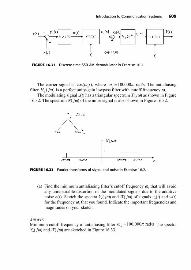
The carrier signal is where rad/s. The antialiasingfilter is a perfect unity-gain lowpass filter with cutoff frequency a.
The modulating signal x(t) has a triangular spectrum X( j ) as shown in Figure16.32. The spectrum N( j ) of the noise signal is also shown in Figure 16.32.
H ja ( )c = 100000cos( ),ct
Introduction to Communication Systems 609
FIGURE 16.31 Discrete-time SSB-AM demodulator in Exercise 16.2.
FIGURE 16.32 Fourier transforms of signal and noise in Exercise 16.2.
(a) Find the minimum antialiasing filter’s cutoff frequency a that will avoidany unrepairable distortion of the modulated signals due to the additivenoise n(t). Sketch the spectra Yn( j ) and W( j ) of signals yn(t) and w(t)for the frequency a that you found. Indicate the important frequencies andmagnitudes on your sketch.
Answer:Minimum cutoff frequency of antialiasing filter: The spectraYn( j ) and W( j ) are sketched in Figure 16.33.
a = 100 000, rad/s
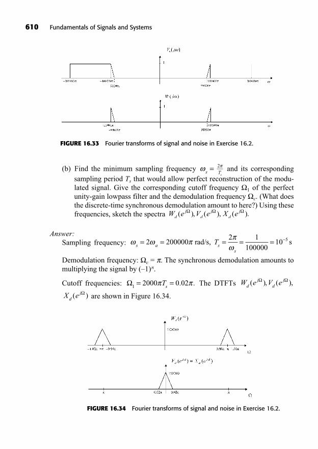
(b) Find the minimum sampling frequency and its correspondingsampling period Ts that would allow perfect reconstruction of the modu-lated signal. Give the corresponding cutoff frequency 1 of the perfectunity-gain lowpass filter and the demodulation frequency c. (What doesthe discrete-time synchronous demodulation amount to here?) Using thesefrequencies, sketch the spectra
Answer:Sampling frequency:
Demodulation frequency: c = . The synchronous demodulation amounts tomultiplying the signal by (–1)n.
Cutoff frequencies: The DTFTs
are shown in Figure 16.34.X edj( )
W e V edj
dj( ), ( ),
1 2000 0 02= =Ts . .
s a ss
T= = = = =2 2000002 1
10000010 5rad/s s,
W e V e X edj
dj
dj( ), ( ), ( ).
sT2
s =
610 Fundamentals of Signals and Systems
FIGURE 16.33 Fourier transforms of signal and noise in Exercise 16.2.
FIGURE 16.34 Fourier transforms of signal and noise in Exercise 16.2.
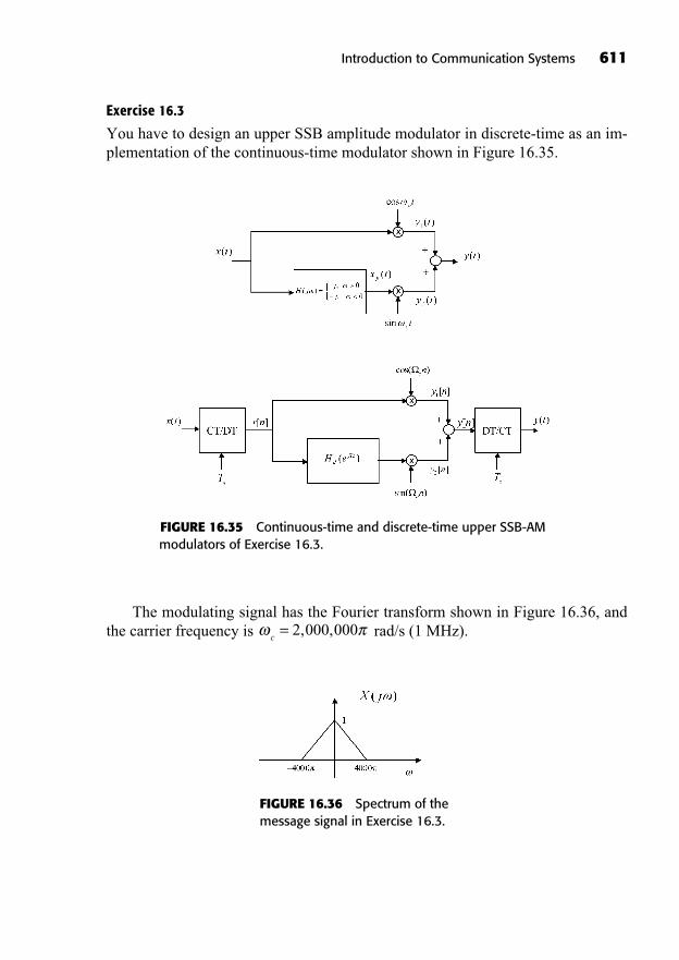
Introduction to Communication Systems 611
Exercise 16.3
You have to design an upper SSB amplitude modulator in discrete-time as an im-plementation of the continuous-time modulator shown in Figure 16.35.
FIGURE 16.35 Continuous-time and discrete-time upper SSB-AM modulators of Exercise 16.3.
The modulating signal has the Fourier transform shown in Figure 16.36, andthe carrier frequency is rad/s (1 MHz).c
= 2 000 000, ,
FIGURE 16.36 Spectrum of themessage signal in Exercise 16.3.
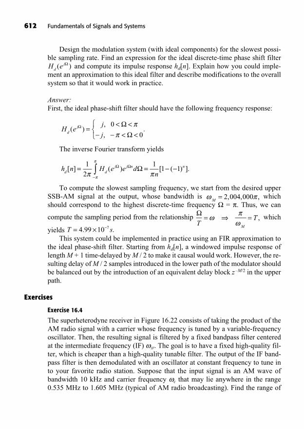
612 Fundamentals of Signals and Systems
Design the modulation system (with ideal components) for the slowest possi-ble sampling rate. Find an expression for the ideal discrete-time phase shift filter
and compute its impulse response hd[n]. Explain how you could imple-ment an approximation to this ideal filter and describe modifications to the overallsystem so that it would work in practice.
Answer:First, the ideal phase-shift filter should have the following frequency response:
The inverse Fourier transform yields
To compute the slowest sampling frequency, we start from the desired upperSSB-AM signal at the output, whose bandwidth is whichshould correspond to the highest discrete-time frequency = . Thus, we can
compute the sampling period from the relationship which
yields This system could be implemented in practice using an FIR approximation to
the ideal phase-shift filter. Starting from hd[n], a windowed impulse response oflength M + 1 time-delayed by M / 2 to make it causal would work. However, the re-sulting delay of M / 2 samples introduced in the lower path of the modulator shouldbe balanced out by the introduction of an equivalent delay block z –M/2 in the upperpath.
Exercises
Exercise 16.4
The superheterodyne receiver in Figure 16.22 consists of taking the product of theAM radio signal with a carrier whose frequency is tuned by a variable-frequencyoscillator. Then, the resulting signal is filtered by a fixed bandpass filter centeredat the intermediate frequency (IF) IF. The goal is to have a fixed high-quality fil-ter, which is cheaper than a high-quality tunable filter. The output of the IF band-pass filter is then demodulated with an oscillator at constant frequency to tune into your favorite radio station. Suppose that the input signal is an AM wave ofbandwidth 10 kHz and carrier frequency c that may lie anywhere in the range0.535 MHz to 1.605 MHz (typical of AM radio broadcasting). Find the range of
T s= ×4 99 10 7. .T
TM
= = ,
M= 2 004 000, , ,
h n H e e dnd d
j j n n[ ] ( ) [ ( ) ].= =1
2
11 1
H ej
jdj( )
,
,.=
< << <
0
0
H ed
j( )
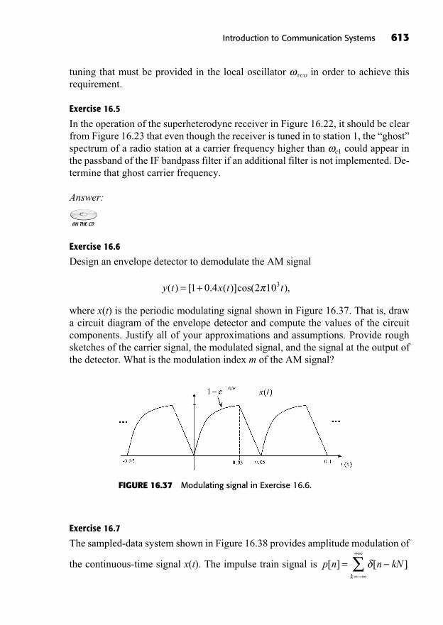
tuning that must be provided in the local oscillator VCO in order to achieve this requirement.
Exercise 16.5
In the operation of the superheterodyne receiver in Figure 16.22, it should be clearfrom Figure 16.23 that even though the receiver is tuned in to station 1, the “ghost”spectrum of a radio station at a carrier frequency higher than c1 could appear inthe passband of the IF bandpass filter if an additional filter is not implemented. De-termine that ghost carrier frequency.
Answer:
Exercise 16.6
Design an envelope detector to demodulate the AM signal
where x(t) is the periodic modulating signal shown in Figure 16.37. That is, drawa circuit diagram of the envelope detector and compute the values of the circuitcomponents. Justify all of your approximations and assumptions. Provide roughsketches of the carrier signal, the modulated signal, and the signal at the output ofthe detector. What is the modulation index m of the AM signal?
y t x t t( ) [ . ( )]cos( ),= +1 0 4 2 103
Introduction to Communication Systems 613
FIGURE 16.37 Modulating signal in Exercise 16.6.
Exercise 16.7
The sampled-data system shown in Figure 16.38 provides amplitude modulation of
the continuous-time signal x(t). The impulse train signal is p n n kNk
[ ] [ ].==
+
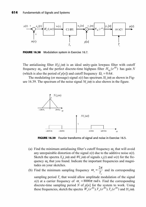
614 Fundamentals of Signals and Systems
FIGURE 16.38 Modulation system in Exercise 16.7.
The antialiasing filter Ha( j ) is an ideal unity-gain lowpass filter with cutoff frequency a, and the perfect discrete-time highpass filter has gain N(which is also the period of p[n]) and cutoff frequency
The modulating (or message) signal x(t) has spectrum X( j ) as shown in Fig-ure 16.39. The spectrum of the noise signal N( j ) is also shown in the figure.
10 6= . .H ehp
j( )
FIGURE 16.39 Fourier transforms of signal and noise in Exercise 16.5.
(a) Find the minimum antialiasing filter’s cutoff frequency a that will avoidany unrepairable distortion of the signal x(t) due to the additive noise n(t).Sketch the spectra Xn( j ) and W( j ) of signals xn(t) and w(t) for the fre-quency a that you found. Indicate the important frequencies and magni-tudes on your sketches.
(b) Find the minimum sampling frequency and its corresponding
sampling period Ts that would allow amplitude modulation of the signalx(t) at a carrier frequency of Find the correspondingdiscrete-time sampling period N of p[n] for the system to work. Usingthese frequencies, sketch the spectra and Y( j ).W e V e Y ed
jd
jd
j( ), ( ), ( )
c= 8000 rad/s.
ssT
= 2
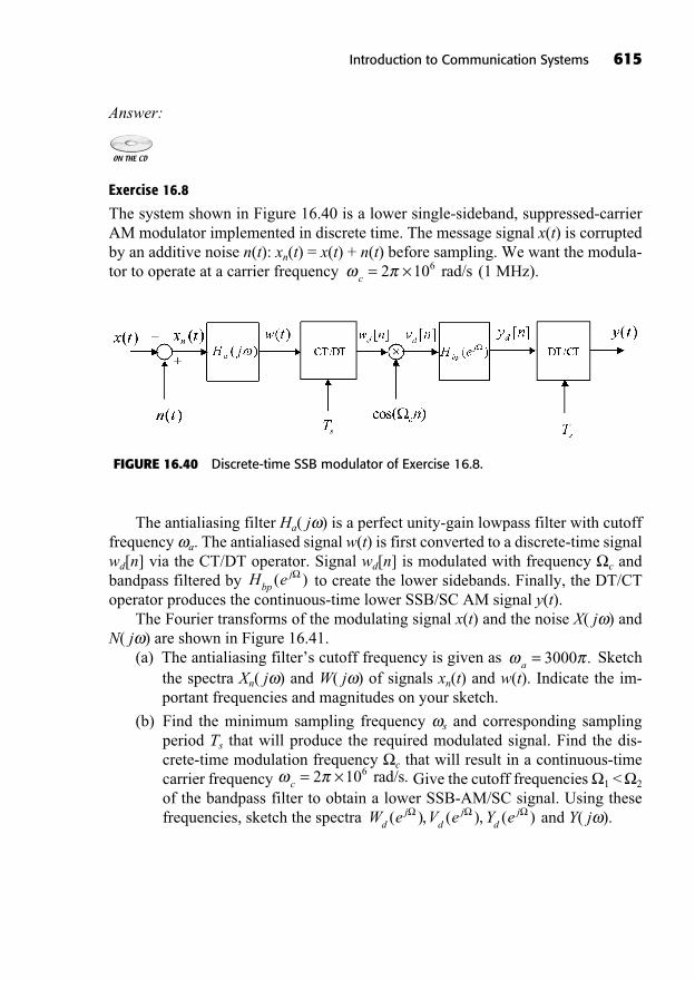
Answer:
Exercise 16.8
The system shown in Figure 16.40 is a lower single-sideband, suppressed-carrierAM modulator implemented in discrete time. The message signal x(t) is corruptedby an additive noise n(t): xn(t) = x(t) + n(t) before sampling. We want the modula-tor to operate at a carrier frequency (1 MHz).c = ×2 106 rad/s
Introduction to Communication Systems 615
FIGURE 16.40 Discrete-time SSB modulator of Exercise 16.8.
The antialiasing filter Ha( j ) is a perfect unity-gain lowpass filter with cutofffrequency a. The antialiased signal w(t) is first converted to a discrete-time signalwd[n] via the CT/DT operator. Signal wd[n] is modulated with frequency c and bandpass filtered by to create the lower sidebands. Finally, the DT/CToperator produces the continuous-time lower SSB/SC AM signal y(t).
The Fourier transforms of the modulating signal x(t) and the noise X( j ) andN( j ) are shown in Figure 16.41.
(a) The antialiasing filter’s cutoff frequency is given as Sketchthe spectra Xn( j ) and W( j ) of signals xn(t) and w(t). Indicate the im-portant frequencies and magnitudes on your sketch.
(b) Find the minimum sampling frequency s and corresponding samplingperiod Ts that will produce the required modulated signal. Find the dis-crete-time modulation frequency c that will result in a continuous-timecarrier frequency Give the cutoff frequencies 1 < 2
of the bandpass filter to obtain a lower SSB-AM/SC signal. Using thesefrequencies, sketch the spectra and Y( j ).W e V e Y ed
jd
jd
j( ), ( ), ( )
c = ×2 106 rad/s.
a = 3000 .
H ebpj( )
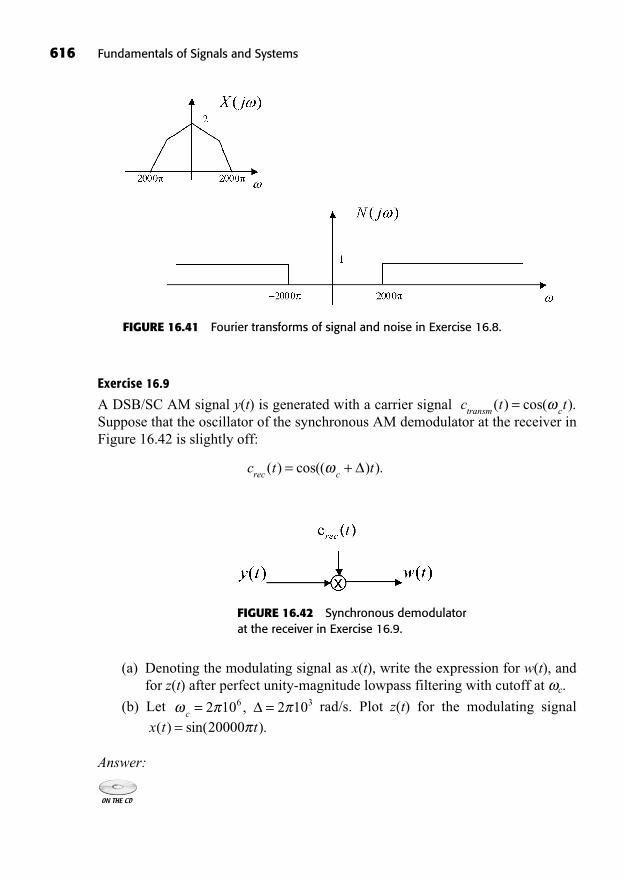
Exercise 16.9
A DSB/SC AM signal y(t) is generated with a carrier signal Suppose that the oscillator of the synchronous AM demodulator at the receiver inFigure 16.42 is slightly off:
c t trec c( ) cos(( ) ).= +
c t ttransm c( ) cos( ).=
616 Fundamentals of Signals and Systems
FIGURE 16.41 Fourier transforms of signal and noise in Exercise 16.8.
FIGURE 16.42 Synchronous demodulatorat the receiver in Exercise 16.9.
(a) Denoting the modulating signal as x(t), write the expression for w(t), andfor z(t) after perfect unity-magnitude lowpass filtering with cutoff at c.
(b) Let rad/s. Plot z(t) for the modulating signal
Answer:
x t t( ) sin( ).= 20000c = =2 10 2 106 3,
617
System Discretization andDiscrete-Time LTI State-Space Models
17
In This Chapter
Controllable Canonical FormObservable Canonical FormZero-State and Zero-Input Responses of a Discrete-Time State-Space Systemz-Transform Solution of Discrete-Time State-Space SystemsDiscretization of Continuous-Time SystemsSummaryTo Probe FurtherExercises
((Lecture 68: State Models of LTI Difference Systems))
In this last chapter, causal discrete-time state-space models of linear time-in-variant (LTI) systems are introduced mainly as a means of providing methodsto discretize continuous-time LTI systems. The topic of system discretization is
an important one for at least two reasons. First, engineers often need to simulate thebehavior of continuous-time systems, and analytical solutions can be very difficultto obtain for systems of order three or more. Second, many filter design and con-troller design techniques have been developed in continuous time. Discretizing the

618 Fundamentals of Signals and Systems
resulting system often yields a sampled-data implementation that performs just aswell as the intended continuous-time design.
Of course, discrete-time LTI (DLTI) state-space models are of interest in theirown right, particularly in advanced multivariable discrete-time filter design andcontroller design techniques, which are beyond the scope of this textbook. An im-portant word on notation before we move on: for discrete-time state-space systems,the input signal is conventionally written as u[n] (not to be confused with the unitstep) instead of x[n], as the latter is used for the vector of state variables. Hence, inthis chapter we will use q[n] to denote the unit step signal.
CONTROLLABLE CANONICAL FORM
In general, an Nth-order linear constant-coefficient causal difference equation withM ≤ N has the form
, (17.1)
which can be expanded into
(17.2)
Just like the continuous-time case, we can derive a state-space model for thissystem by first finding its controllable canonical form (direct form) realization. Wetake the intermediate variable w[n] and its successive delayed versions asstate variables. Let without loss of generality. Taking the z-transform onboth sides of the difference Equation 17.1, we obtain the transfer function (with re-gion of convergence [ROC] the exterior of a disk of radius equal to the magnitudeof the outermost pole):
(17.3)
H zY zU z
b z
a z
b b z
kk
k
M
kk
k
N( )
( )( )
= =
=+
=
=
0
0
0 11
+ ++ + + +
+
+
b z b z
a z a z a zM
MM
M
NN
NN
11
11
111
..
a0 1=N 1
a y n a y n a y n N b x n b x nN0 1 0 1
1 1[ ] [ ] [ ] [ ] [ ]+ + + = + + + b x n MM
[ ].
a y n k b x n kk
N
k
M
[ ] [ ]=
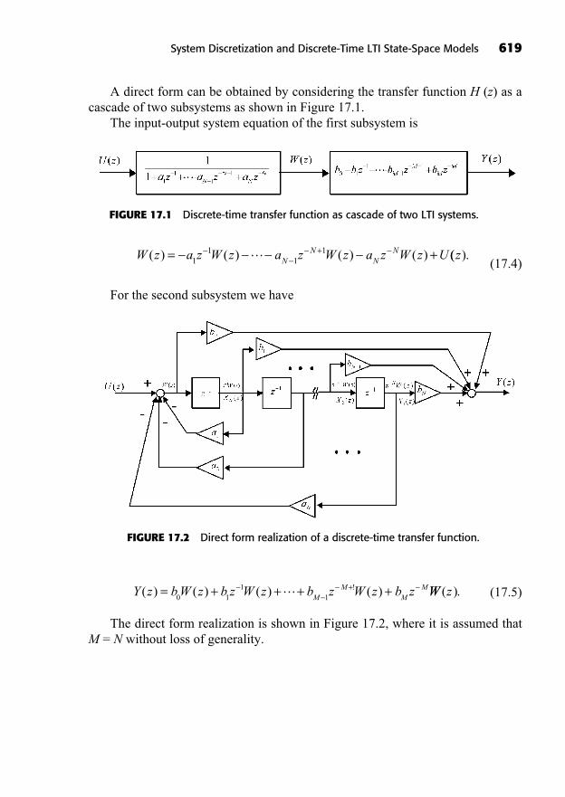
A direct form can be obtained by considering the transfer function H (z) as acascade of two subsystems as shown in Figure 17.1.
The input-output system equation of the first subsystem is
(17.4)
For the second subsystem we have
(17.5)
The direct form realization is shown in Figure 17.2, where it is assumed thatM = N without loss of generality.
Y z b W z b z W z b z W z b zM
MM
M( ) ( ) ( ) ( )!= + + + ++0 1
11
WW z( ).
W z a z W z a z W z a z W z UNN
NN( ) ( ) ( ) ( )= ++
11
11 (( ).z
System Discretization and Discrete-Time LTI State-Space Models 619
FIGURE 17.1 Discrete-time transfer function as cascade of two LTI systems.
FIGURE 17.2 Direct form realization of a discrete-time transfer function.
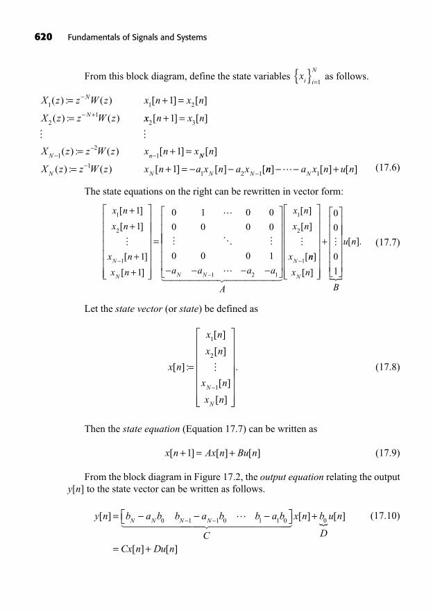
620 Fundamentals of Signals and Systems
From this block diagram, define the state variables as follows.
(17.6)
The state equations on the right can be rewritten in vector form:
(17.7)
Let the state vector (or state) be defined as
(17.8)
Then the state equation (Equation 17.7) can be written as
(17.9)
From the block diagram in Figure 17.2, the output equation relating the outputy[n] to the state vector can be written as follows.
(17.10)y n b a b b a b b a b
C
N N N N[ ] = 0 1 1 0 1 1 0� ���������� ��������� �x n b
D
u n
Cx n Du n
[ ] [ ]
[ ] [ ]
+
= +
0
x n Ax n Bu n[ ] [ ] [ ]+ = +1
x n
x n
x n
x n
x nN
N
[ ] :
[ ]
[ ]
[ ]
[ ]
=
1
2
1
� .
x n
x n
x n
x nN
N
1
2
1
1
1
1
1
[ ]
[ ]
[ ]
[ ]
+
+
+
+
� =
0 1 0 0
0 0 0 0
0 0 0 1
1 2 1
� � �
a a a aN N
A
x n
x n
xN
� ������ ������
�
1
2
1
[ ]
[ ]
[nn
x nN
]
[ ]
+
0
0
0
1
�
B
u n
�
[ ].
X z z W z x n x n
X z z W z
N
N
1 1 2
21
1( ) : ( ) [ ] [ ]
( ) : ( )
= + =
= + xx n x n
X z z W z x n xN n
2 3
12
1
1
1
[ ] [ ]
( ) : ( ) [ ]
+ =
= + =� �
NN
N N N N
n
X z z W z x n a x n a x
[ ]
( ) : ( ) [ ] [ ] [= + =11 2 11 nn a x n u nN] [ ] [ ]+ 1
xi i
N{ } =1
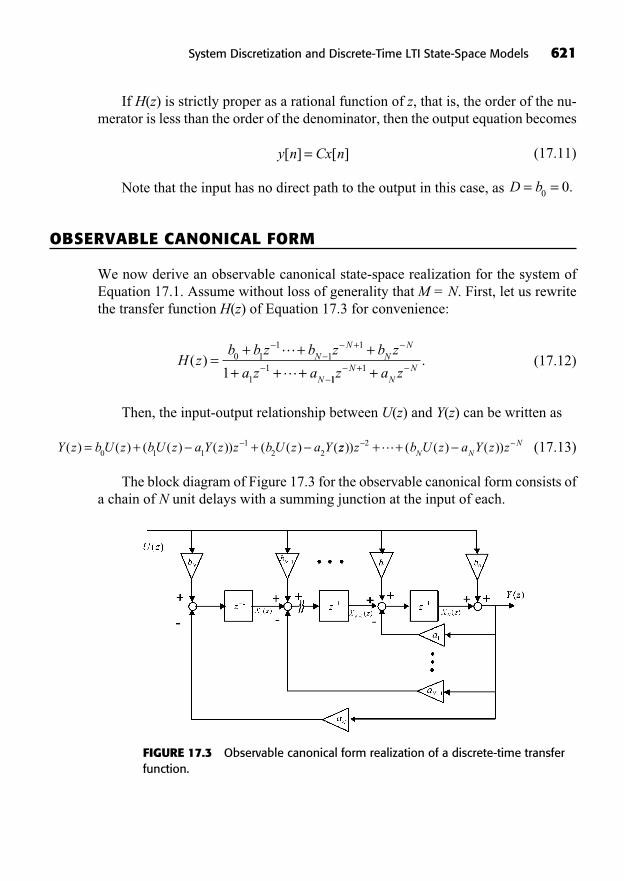
If H(z) is strictly proper as a rational function of z, that is, the order of the nu-merator is less than the order of the denominator, then the output equation becomes
(17.11)
Note that the input has no direct path to the output in this case, as
OBSERVABLE CANONICAL FORM
We now derive an observable canonical state-space realization for the system ofEquation 17.1. Assume without loss of generality that M = N. First, let us rewritethe transfer function H(z) of Equation 17.3 for convenience:
(17.12)
Then, the input-output relationship between U(z) and Y(z) can be written as
(17.13)
The block diagram of Figure 17.3 for the observable canonical form consists ofa chain of N unit delays with a summing junction at the input of each.
Y z b U z bU z a Y z z b U z a Y( ) ( ) ( ( ) ( )) ( ( ) (= + +0 1 11
2 2 zz z b U z a Y z zN NN)) ( ( ) ( ))+ +2
H zb b z b z b z
a z aN
NN
N
N
( ) =+ + +
+ + +
+0 1
11
1
111
111z a zN
NN+ +
.
D b= =0 0.
y n Cx n[ ] [ ]=
System Discretization and Discrete-Time LTI State-Space Models 621
FIGURE 17.3 Observable canonical form realization of a discrete-time transferfunction.
The state variables are defined as the outputs of the unit delays, which gives us:
(17.14)
The state equations on the right can be rewritten in vector form:
(17.15)
Again this state equation can be written as in Equation 17.9. From the block di-agram in Figure 17.3, the output equation relating the output y[n] to the state vec-tor can be written as follows.
(17.16)
((Lecture 69: Zero-State and Zero-Input Responses of Discrete-Time State Models))
ZERO-STATE AND ZERO-INPUT RESPONSES OF A DISCRETE-TIME STATE-SPACE SYSTEM
Recall that the response of a causal LTI difference system with nonzero initial conditions is composed of a zero-state response due to the input signal only and a
y n
C
x n b
D
u n
Cx n
[ ] [ ] [ ]
[ ]
= +
=
0 0 0 1 0� ���� ���� �
++ Du n[ ]
x n
x n
x n
x nN
N
1
2
1
1
1
1
1
[ ]
[ ]
[ ]
[ ]
+
+
+
+
� =
0 0 0
1 0 0
0 0 0
0 0 1
1
2
1
� � �
a
a
a
a
N
N
A
x n
x n
xN
� ����� �����
�
1
2
1
[ ]
[ ]
[nn
x n
b a b
b a
N
N N
N N
]
[ ]
+
0
1 1bb
b a b
b a b
B
0
2 2 0
1 1 0
�
� ��� ����
u n[ ].
zX z a X z b a b U z x n a xN N N N N N1 0 1 1( ) ( ) ( ) ( ) [ ] [= + + = nn b a b u n
zX z X z a X z bN N
N N N
] ( ) [ ]
( ) ( ) ( ) (
+
= +0
2 1 1 + = +1 1 0 2 1 11a b U z x n x n a x n bN N N N) ( ) [ ] [ ] [ ] ( 11 1 0
3 2 2 2= +
a b u n
zX z X z a X z bN
N N N
) [ ]
( ) ( ) ( ) ( aa b U z x n x n a x n bN N N N+ = +2 0 3 2 2 21) ( ) [ ] [ ] [ ] ( aa b u n
zX z X z a X z b a
N
N N N= +
2 0
1 1 1 1
) [ ]
( ) ( ) ( ) (
� �bb U z x n x n a x n b a b uN N N0 1 1 1 1 01) ( ) [ ] [ ] [ ] ( ) [+ = + nn]
.
622 Fundamentals of Signals and Systems
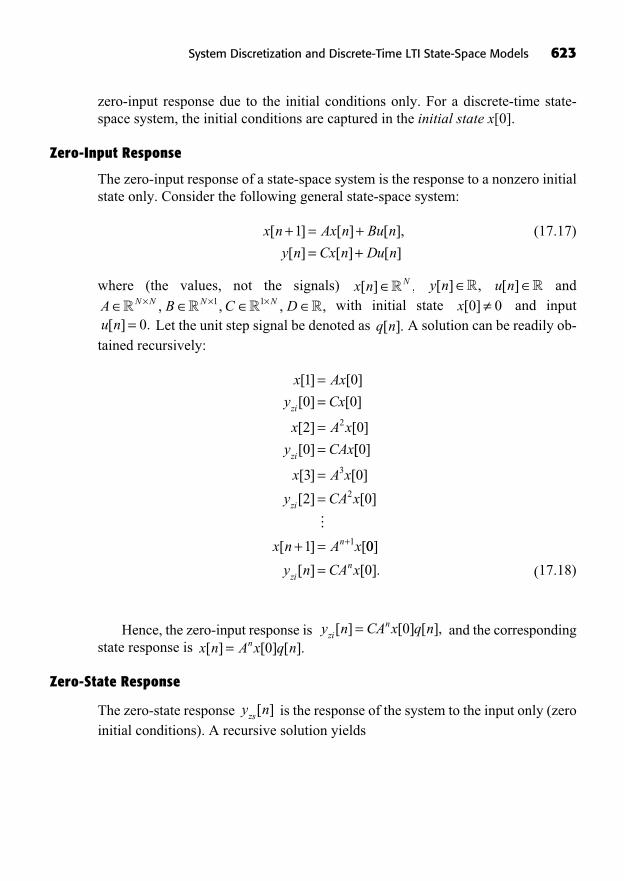
zero-input response due to the initial conditions only. For a discrete-time state-space system, the initial conditions are captured in the initial state x[0].
Zero-Input Response
The zero-input response of a state-space system is the response to a nonzero initialstate only. Consider the following general state-space system:
(17.17)
where (the values, not the signals) and with initial state and input
Let the unit step signal be denoted as A solution can be readily ob-tained recursively:
(17.18)
Hence, the zero-input response is and the correspondingstate response is
Zero-State Response
The zero-state response is the response of the system to the input only (zeroinitial conditions). A recursive solution yields
y nzs[ ]
x n A x q nn[ ] [ ] [ ].= 0y n CA x q nzi
n[ ] [ ] [ ],= 0
x Ax
y Cx
x A x
y CAx
zi
zi
[ ] [ ]
[ ] [ ]
[ ] [ ]
[ ]
1 0
0 0
2 0
0
2
==
== [[ ]
[ ] [ ]
[ ] [ ]
[ ] [
0
3 0
2 0
1
3
2
1
x A x
y CA x
x n A x
zi
n
==
+ = +
�
00
0
]
[ ] [ ].y n CA xzin=
q n[ ].u n[ ] .= 0x[ ]0 0A B C DN N N N× × ×� � � �, , , ,1 1
u n[ ] �y n[ ] ,�x n N[ ] ,�
x n Ax n Bu n
y n Cx n Du n
[ ] [ ] [ ],
[ ] [ ] [ ]
+ = += +
1
System Discretization and Discrete-Time LTI State-Space Models 623
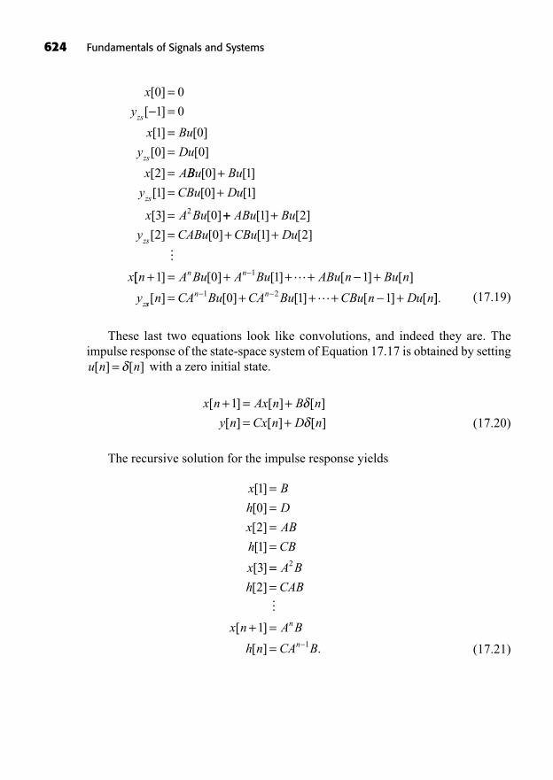
(17.19)
These last two equations look like convolutions, and indeed they are. The impulse response of the state-space system of Equation 17.17 is obtained by setting
with a zero initial state.
(17.20)
The recursive solution for the impulse response yields
(17.21)
x B
h D
x AB
h CB
x
[ ]
[ ]
[ ]
[ ]
[ ]
1
0
2
1
3
=======
+ ==
A B
h CAB
x n A B
h n CA B
n
n
2
1
2
1
[ ]
[ ]
[ ] .
�
x n Ax n B n
y n Cx n D n
[ ] [ ] [ ]
[ ] [ ] [ ]
+ = += +
1
u n n[ ] [ ]=
x
y
x Bu
y Du
x A
zs
zs
[ ]
[ ]
[ ] [ ]
[ ] [ ]
[ ]
0 0
1 0
1 0
0 0
2
==
==
= BBu Bu
y CBu Du
x A Bu
zs
[ ] [ ]
[ ] [ ] [ ]
[ ] [ ]
0 1
1 0 1
3 02
+= +
= ++ += + +
ABu Bu
y CABu CBu Du
x
zs
[ ] [ ]
[ ] [ ] [ ] [ ]
1 2
2 0 1 2
�
[[ ] [ ] [ ] [ ] [ ]n A Bu A Bu ABu n Bu n
y
n n
z
+ = + + + +1 0 1 11
ssn nn CA Bu CA Bu CBu n Du n[ ] [ ] [ ] [ ] [= + + + +1 20 1 1 ]].
624 Fundamentals of Signals and Systems
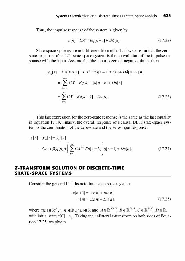
Thus, the impulse response of the system is given by
(17.22)
State-space systems are not different from other LTI systems, in that the zero-state response of an LTI state-space system is the convolution of the impulse re-sponse with the input. Assume that the input is zero at negative times, then
(17.23)
This last expression for the zero-state response is the same as the last equalityin Equation 17.19. Finally, the overall response of a causal DLTI state-space sys-tem is the combination of the zero-state and the zero-input response:
(17.24)
Z-TRANSFORM SOLUTION OF DISCRETE-TIME STATE-SPACE SYSTEMS
Consider the general LTI discrete-time state-space system:
(17.25)
where and with initial state Taking the unilateral z-transform on both sides of Equa-tion 17.25, we obtain
x x[ ] .0 0=A B C DN N N N× × ×� � � �, , , ,1 1x n y n u nN[ ] , [ ] , [ ]� � �
x n Ax n Bu n
y n Cx n Du n
[ ] [ ] [ ]
[ ] [ ] [ ],
+ = += +
1
y n y n y n
CA x q n CA Bu n k
zi zs
n k
[ ] [ ] [ ]
[ ] [ ] [ ]
= +
= +0 1
kk
n
q n Du n=
+1
1[ ] [ ].
y n h n u n CA Bq n u n D n uzsn[ ] [ ] [ ] [ ] [ ] [ ] [= = +1 1 nn
CA Bq k u n k Du n
CA Bu
k
k
k
]
[ ] [ ] [ ]= +
=
=
+1
1
1
[[ ] [ ].n k Du nk
n
+=1
h n CA Bq n D nn[ ] [ ] [ ].= +1 1
System Discretization and Discrete-Time LTI State-Space Models 625
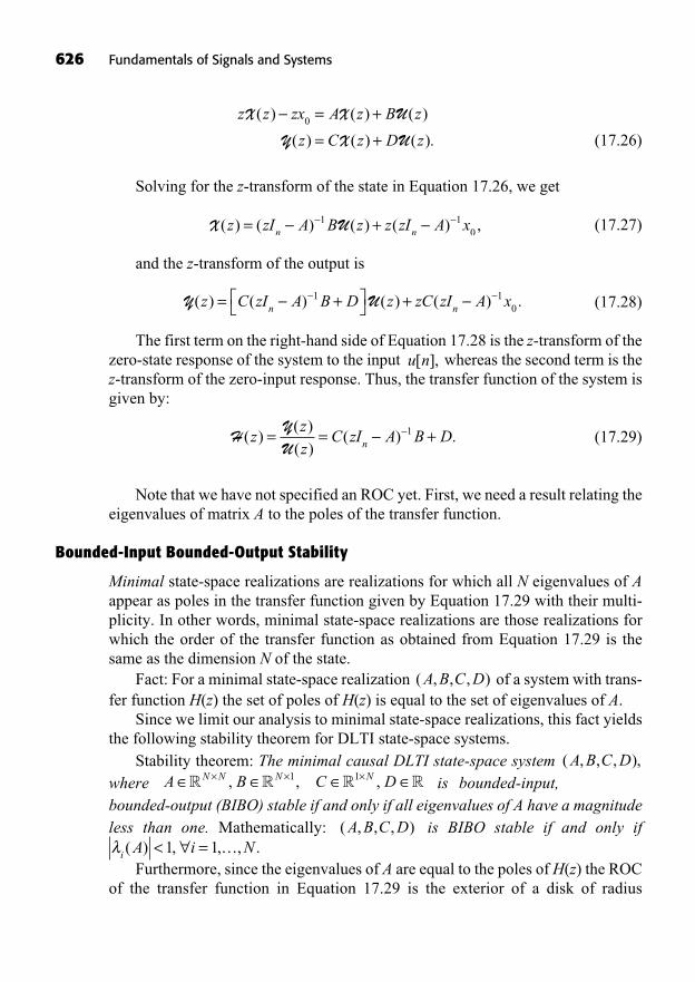
(17.26)
Solving for the z-transform of the state in Equation 17.26, we get
(17.27)
and the z-transform of the output is
(17.28)
The first term on the right-hand side of Equation 17.28 is the z-transform of thezero-state response of the system to the input whereas the second term is thez-transform of the zero-input response. Thus, the transfer function of the system isgiven by:
(17.29)
Note that we have not specified an ROC yet. First, we need a result relating theeigenvalues of matrix A to the poles of the transfer function.
Bounded-Input Bounded-Output Stability
Minimal state-space realizations are realizations for which all N eigenvalues of Aappear as poles in the transfer function given by Equation 17.29 with their multi-plicity. In other words, minimal state-space realizations are those realizations forwhich the order of the transfer function as obtained from Equation 17.29 is thesame as the dimension N of the state.
Fact: For a minimal state-space realization of a system with trans-fer function H(z) the set of poles of H(z) is equal to the set of eigenvalues of A.
Since we limit our analysis to minimal state-space realizations, this fact yieldsthe following stability theorem for DLTI state-space systems.
Stability theorem: The minimal causal DLTI state-space system where is bounded-input,bounded-output (BIBO) stable if and only if all eigenvalues of A have a magnitudeless than one. Mathematically: is BIBO stable if and only if
Furthermore, since the eigenvalues of A are equal to the poles of H(z) the ROCof the transfer function in Equation 17.29 is the exterior of a disk of radius
i A i N( ) , , , .< =1 1…( , , , )A B C D
C DN×� �1 ,A BN N N× ×� �, ,1( , , , ),A B C D
( , , , )A B C D
HYU
( )( )( )
( ) .zzz
C zI A B Dn= = +1
u n[ ],
Y U( ) ( ) ( ) ( ) .z C zI A B D z zC zI A xn n= + +1 10
X U( ) ( ) ( ) ( ) ,z zI A B z z zI A xn n= +1 10
z z zx A z B z
z C z D z
X X U
Y X U
( ) ( ) ( )
( ) ( ) ( ).
= +
= +0
626 Fundamentals of Signals and Systems
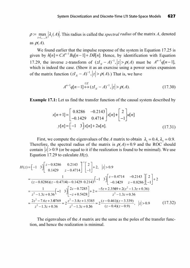
This radius is called the spectral radius of the matrix A, denoted
as
We found earlier that the impulse response of the system in Equation 17.25 isgiven by Hence, by identification with Equation
17.29, the inverse z-transform of must be which is indeed the case. (Show it as an exercise using a power series expansion
of the matrix function ) That is, we have
(17.30)
Example 17.1: Let us find the transfer function of the causal system described by
(17.31)
First, we compute the eigenvalues of the A matrix to obtain Therefore, the spectral radius of the matrix is and the ROC should contain (or be equal to it if the realization is found to be minimal). We useEquation 17.29 to calculate H(z).
(17.32)
The eigenvalues of the A matrix are the same as the poles of the transfer func-tion, and hence the realization is minimal.
H zz
z( )
. .
. .= 1 3
0 8286 0 2143
0 1429 0 4714+ >
=
12
12 0 9
10 8286 0 471
, .
( . )( .
z
z z 44 0 1429 0 21431 3
0 4714 0 2143
0 1) . .
. .
.
z
4429 0 8286
2
12
1
1 3 0 362
z
z z
+
=+
.
. . ++ = +
1 32 0 7285
0 54282
5 2 35z
z
z.
.
. 669 2 1 3 0 36
1 3 0 36
2 7 6 3
2
2
2
+ ++
= +
( . . )
. .
. .
z z
z z
z z 00769
1 3 0 362
3 8 1 5385
1 3 02
2
2z z
z z
z z+= +
+. .
. .
. .3362
0 461 3 3390 4 0 9
0 9= >( . )( . )( . )( . )
, .z z
z zz
z > 0 9.( ) .A = 0 9
1 20 4 0 9= =. , . .
x n x n[ ]. .
. .[ ]+ =1
0 8286 0 2143
0 1429 0 4714++
= +
2
1
1 3 2
u n
y n x n u n
[ ]
[ ] [ ] [ ].
A q n zI A z AnUZ
N >1 11[ ] ( ) , ( ).
( ) , ( ).zI A z AN >1
A q nn 1 1[ ],( ) , ( )zI A z AN >1
h n CA Bq n D nn[ ] [ ] [ ].= +1 1
( ).A
: max ( ) ., ,
==i N i A
1…
System Discretization and Discrete-Time LTI State-Space Models 627
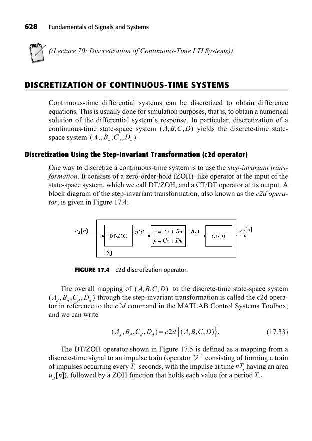
((Lecture 70: Discretization of Continuous-Time LTI Systems))
DISCRETIZATION OF CONTINUOUS-TIME SYSTEMS
Continuous-time differential systems can be discretized to obtain difference equations. This is usually done for simulation purposes, that is, to obtain a numericalsolution of the differential system’s response. In particular, discretization of a continuous-time state-space system yields the discrete-time state-space system
Discretization Using the Step-Invariant Transformation (c2d operator)
One way to discretize a continuous-time system is to use the step-invariant trans-formation. It consists of a zero-order-hold (ZOH)–like operator at the input of thestate-space system, which we call DT/ZOH, and a CT/DT operator at its output. Ablock diagram of the step-invariant transformation, also known as the c2d opera-tor, is given in Figure 17.4.
The overall mapping of to the discrete-time state-space systemthrough the step-invariant transformation is called the c2d opera-
tor in reference to the c2d command in the MATLAB Control Systems Toolbox,and we can write
(17.33)
The DT/ZOH operator shown in Figure 17.5 is defined as a mapping from adiscrete-time signal to an impulse train (operator consisting of forming a trainof impulses occurring every seconds, with the impulse at time having an area
followed by a ZOH function that holds each value for a period Ts.u nd [ ]),
nTsT
s
V 1
( , , , ) ( , , , ) .A B C D c d A B C Dd d d d = { }2
( , , , )A B C Dd d d d
( , , , )A B C D
( , , , ).A B C Dd d d d
( , , , )A B C D
628 Fundamentals of Signals and Systems
FIGURE 17.4 c2d discretization operator.
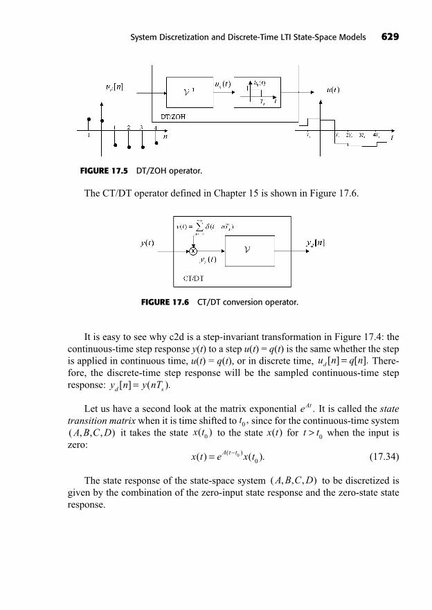
The CT/DT operator defined in Chapter 15 is shown in Figure 17.6.
It is easy to see why c2d is a step-invariant transformation in Figure 17.4: thecontinuous-time step response y(t) to a step u(t) = q(t) is the same whether the stepis applied in continuous time, u(t) = q(t), or in discrete time, There-fore, the discrete-time step response will be the sampled continuous-time step response:
Let us have a second look at the matrix exponential It is called the statetransition matrix when it is time shifted to since for the continuous-time system
it takes the state to the state for when the input iszero:
(17.34)
The state response of the state-space system to be discretized isgiven by the combination of the zero-input state response and the zero-state stateresponse.
( , , , )A B C D
x t e x tA t t( ) ( ).( )= 00
t t> 0x t( )x t( )0( , , , )A B C Dt0 ,
eAt .
y n y nTd s[ ] ( ).=
u n q nd [ ] [ ].=
System Discretization and Discrete-Time LTI State-Space Models 629
FIGURE 17.5 DT/ZOH operator.
FIGURE 17.6 CT/DT conversion operator.
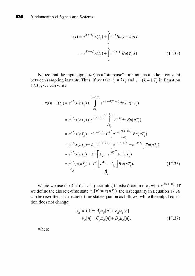
(17.35)
Notice that the input signal u(t) is a “staircase” function, as it is held constantbetween sampling instants. Thus, if we take and in Equation17.35, we can write
(17.36)
where we use the fact that A–1 (assuming it exists) commutes with Ifwe define the discrete-time state the last equality in Equation 17.36can be rewritten as a discrete-time state equation as follows, while the output equa-tion does not change:
(17.37)
where
x n A x n B u n
y n C x n D u nd d d d d
d d d d d
[ ] [ ] [ ]
[ ] [ ] [
+ = +
= +
1
]],
x n x nTd s[ ] : ( ),=eA n Ts( ) .+1
x n T e x nT e dsAT
sA n T
nT
n
s s
s
(( ) ) ( ) (( ) )
(
+ = + ++
1 1
11
1
)
( )
( )
( )
T
s
ATs
A n T A
nT
s
s s
s
Bu nT
e x nT e e d= + +(( )
( )
( )
( )
n T
s
ATs
A n T A
s
s s
Bu nT
e x nT e A e
+
+=
1
1 1
=
+
+
nT
n T
s
ATs
A n
s
s
s
Bu nT
e x nT A e
( )
(
( )
( )
1
1 11 1) ( ) ( )
(
T A n T AnTs
ATs
s s s
s
e e Bu nT
e x nT
+
= )) ( )
( )= +
A I e Bu nT
eA
x nT A e
NAT
s
AT
d
s
s
s
1
1�
AATN
d
ss I B
B
u nT� ��� ���
( ).
t k Ts= +( )1t kTs0 =
x t e x t e Bu t d
e
A t t A
t
t
A t t
( ) ( ) ( )( )
(
= +
=
0
0
0
0
)) ( )( ) ( )x t e Bu dA t
t
t
0
0
+
630 Fundamentals of Signals and Systems
(17.38)
Discretization Using the Bilinear Transformation
The bilinear transformation (also called Tustin’s method) is a mapping from theLaplace domain to the z-domain via
(17.39)
Example 17.2: Let us discretize the causal first-order lag using
a sampling period of using the bilinear transformation. We have
(17.40)
The DC gain of this discretized system is given by
and hence both systems have the same
low-frequency gain. In fact, the bilinear transformation provides a very good ap-proximation to the frequency response of the continuous-time transfer function, atleast up to frequencies close to the Nyquist rate as seen in the Bode plots of-Figure 17.7.
s2,
H e H H jd
jd
( ) ( ) ( ),0 121 19
101 991 0= = = =
H zs
s
z
zd
sz
z
( ) =++
=+
+=
+
1
1 5
1 201
1
1201
1
1
1
1
1 +++
=+ ++ +
1001
1
1 20 20
1 100 1001
1
1 1
1z
z
z z
z zz
z
z
z= =
1
1
1
121 19
101 99
0 2079 1 0 9048. ( . )
(11 0 98020 9802
1>
. ), .
zz
T ss= 0 1.
H ss
s( ) =
++1
5 1
sT
z
zs
=+
2 1
1
1
1.
A e
B A e I B
C C
D D
dAT
dAT
N
d
d
s
s
:
:
:
: .
=
=
=
=
1
System Discretization and Discrete-Time LTI State-Space Models 631
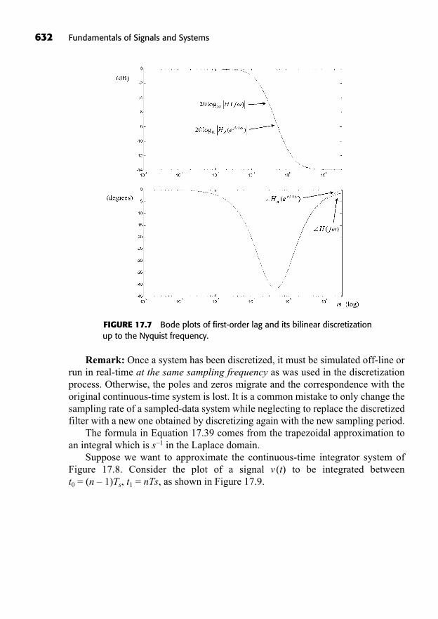
Remark: Once a system has been discretized, it must be simulated off-line orrun in real-time at the same sampling frequency as was used in the discretizationprocess. Otherwise, the poles and zeros migrate and the correspondence with theoriginal continuous-time system is lost. It is a common mistake to only change thesampling rate of a sampled-data system while neglecting to replace the discretizedfilter with a new one obtained by discretizing again with the new sampling period.
The formula in Equation 17.39 comes from the trapezoidal approximation toan integral which is s–1 in the Laplace domain.
Suppose we want to approximate the continuous-time integrator system of Figure 17.8. Consider the plot of a signal v (t) to be integrated between t0 = (n – 1)Ts, t1 = nTs, as shown in Figure 17.9.
632 Fundamentals of Signals and Systems
FIGURE 17.7 Bode plots of first-order lag and its bilinear discretization up to the Nyquist frequency.

The trapezoidal approximation of the integral system s–1 is given by
(17.41)
which in discrete time can be written as (taking the approximation as an equality)
(17.42)
In the z-domain, the transfer function of this system is given by
Thus, we have and Equation 17.39 follows.
Now, applying this bilinear transformation to the state equation of our continuous-time state-space system in the Laplace domain
(17.43)
sX s AX s BU s
Y s CX s DU s
( ) ( ) ( )
( ) ( ) ( ),
= += +
12
1
1
1
1sT z
z= +
,
T z
zs
21
1
1
1
+.
y n y nT
v n v nd ds
d d[ ] [ ] [ ] [ ] .= +12
1
y nT y n T v t dtT
v nTs sn T
nT
s
s
s
( ) (( ) ) ( ) (( )
=12
1ss sv n T) (( ) ) ,+ 1
System Discretization and Discrete-Time LTI State-Space Models 633
FIGURE 17.8 Integrator system.
FIGURE 17.9 Trapezoidal approximation to an integral.
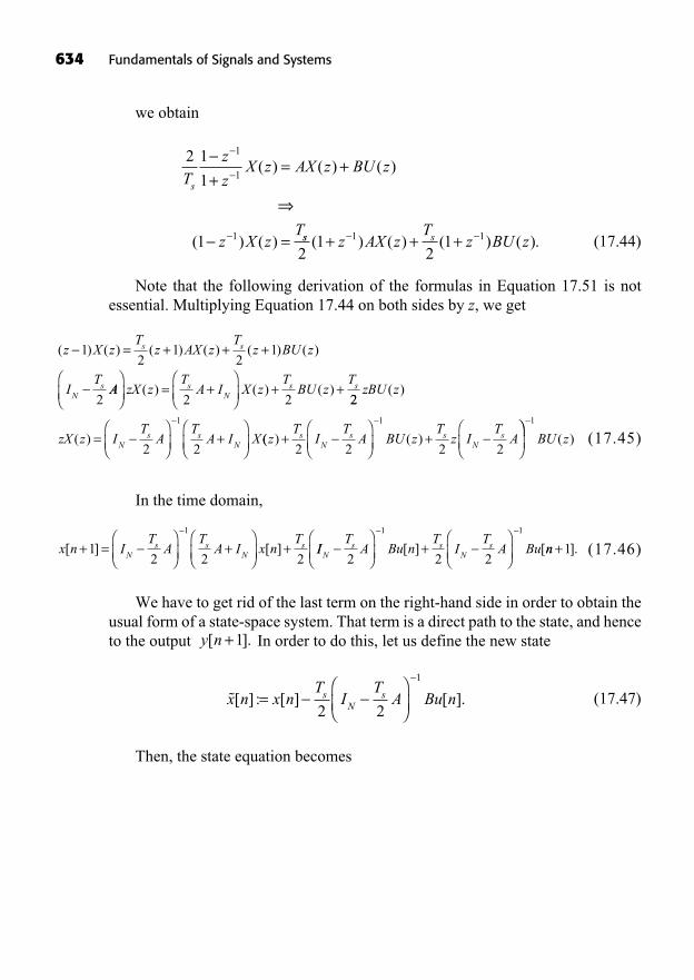
we obtain
(17.44)
Note that the following derivation of the formulas in Equation 17.51 is not essential. Multiplying Equation 17.44 on both sides by z, we get
(17.45)
In the time domain,
(17.46)
We have to get rid of the last term on the right-hand side in order to obtain theusual form of a state-space system. That term is a direct path to the state, and henceto the output In order to do this, let us define the new state
(17.47)
Then, the state equation becomes
x n x nT
IT
A Bu nsN
s[ ] : [ ] [ ].=2 2
1
y n[ ].+1
x n IT
AT
A I x nT
Ns s
Ns[ ] [ ]+ = + +1
2 2 2
1
IIT
A Bu nT
IT
A BuNs s
Ns+
2 2 2
1 1
[ ] [nn +1].
( ) ( ) ( ) ( ) ( ) ( )z X zT
z AX zT
z BU z
IT
s s
Ns
= + + +12
12
1
2AA zX z
TA I X z
TBU z
TsN
s s= + + +( ) ( ) ( )2 2 22
2 2
1
zBU z
zX z IT
AT
A I XNs s
N
( )
( ) = + (( ) ( )zT
IT
A BU zT
z IT
AsN
s sN
s+ +2 2 2 2
1 1
BU z( )
2 1
1
1
1
1
1
Tz
zX z AX z BU z
z X zT
s += +
=
( ) ( ) ( )
( ) ( ) ss sz AX zT
z BU z2
12
11 1( ) ( ) ( ) ( ).+ + +
634 Fundamentals of Signals and Systems
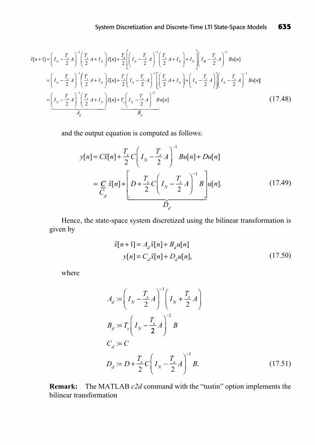
(17.48)
and the output equation is computed as follows:
(17.49)
Hence, the state-space system discretized using the bilinear transformation isgiven by
(17.50)
where
(17.51)
Remark: The MATLAB c2d command with the “tustin” option implements thebilinear transformation
A IT
A IT
A
B T IT
d Ns
Ns
d s Ns
:
:
= +
=
2 2
1
22
2 2
2
1
A B
C C
D DT
C IT
A B
d
ds
Ns
=
= +
:
: ..
x n A x n B u n
y n C x n D u nd d
d d
[ ] [ ] [ ]
[ ] [ ] [ ],
+ = +
= +
1
y n Cx nT
C IT
A Bu n Du nsN
s[ ] [ ] [ ] [ ]= + +
=
2 2
1
CCC
x n DT
C IT
A B
Dd
sN
s
d
� [ ]+ +2 2
1
�� ������ ������
u n[ ].
x n IT
AT
A I x nT
Ns s
N[ ] [ ]+ = + +12 2
1
ssN
s sN NI
TA
TA I I I
2 2 2
1
+ + NNs
Ns s
N
TA Bu n
IT
AT
A I= +
2
2 2
1
1
[ ]
+ + x nT
IT
AT
A IsN
s sN[ ]
2 2 2
1
+ IT
A IT
A Bu nNs
Ns
2 2
1
[ ]]
= +IT
AT
A I
A
Ns s
N
d
2 2
1
� ����� ������
� ���� ����x n T I
TA B
B
u ns Ns
d
[ ] [ ]+2
2
System Discretization and Discrete-Time LTI State-Space Models 635
(17.52)
with different Bd and Cd matrices from those given in Equation 17.51 but yield-ing the same transfer function as the state-space realization. Either realization canbe used.
SUMMARY
This chapter introduced discrete-time state-space LTI systems and the discretiza-tion of continuous-time systems.
Difference LTI systems represented by proper rational transfer functions canbe realized as state-space systems. We gave procedures to compute the con-trollable and the observable canonical realizations, but just like the continuous-time case, there exist infinitely many realizations of any given proper rationaltransfer function.We derived the formulas for the zero-input and zero-state responses, the im-pulse response, and the transfer function of a general discrete-time state-spacesystem.A minimal state-space system was shown to be BIBO stable if and only if all of the eigenvalues of its A matrix lie in the open unit disk centered at the origin.Two system discretization techniques were derived: the step-invariant trans-formation, called c2d, and the bilinear transformation.
A IT
A IT
A
B IT
A
d Ns
Ns
d Ns
= +
=
2 2
2
1
=
= +
1
1
2
2
B
C CT IT
A
D DT
C IT
d s Ns
ds
Ns
22
1
A B
636 Fundamentals of Signals and Systems
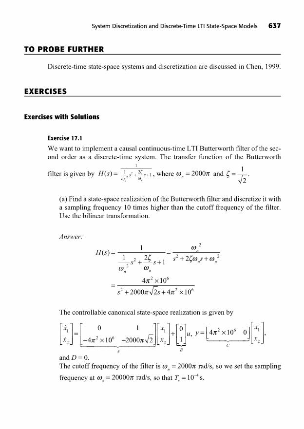
TO PROBE FURTHER
Discrete-time state-space systems and discretization are discussed in Chen, 1999.
EXERCISES
Exercises with Solutions
Exercise 17.1
We want to implement a causal continuous-time LTI Butterworth filter of the sec-ond order as a discrete-time system. The transfer function of the Butterworth
filter is given by , where and
(a) Find a state-space realization of the Butterworth filter and discretize it witha sampling frequency 10 times higher than the cutoff frequency of the filter.Use the bilinear transformation.
Answer:
The controllable canonical state-space realization is given by
and D = 0.The cutoff frequency of the filter is so we set the sampling
frequency at so that Ts= 10 4 s.s
= 20000 rad/s,n= 2000 rad/s,
yx
xC
= ×4 10 02 6 1
2� ��� ���,
�
�� �
x
x
A
1
22 6
0 1
4 10 2000 2=
����� ����� �
x
xu
B
1
2
0
1+ ,
H ss s s s
n n
n
n n
( ) =+ +
=+ +
= ×
11 2
1 2
4
22
2
2 2
2 110
2000 2 4 10
6
2 2 6s s+ + ×
=1
2.n
= 2000s sn n
+ +
11 2
12
2H s( ) =
System Discretization and Discrete-Time LTI State-Space Models 637
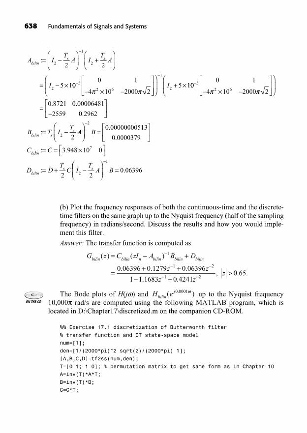
(b) Plot the frequency responses of both the continuous-time and the discrete-time filters on the same graph up to the Nyquist frequency (half of the samplingfrequency) in radians/second. Discuss the results and how you would imple-ment this filter.
Answer: The transfer function is computed as
The Bode plots of H(j ) and up to the Nyquist frequency10,000 rad/s are computed using the following MATLAB program, which is located in D:\Chapter17\discretized.m on the companion CD-ROM.
%% Exercise 17.1 discretization of Butterworth filter
% transfer function and CT state-space model
num=[1];
den=[1/(2000*pi)^2 sqrt(2)/(2000*pi) 1];
[A,B,C,D]=tf2ss(num,den);
T=[0 1; 1 0]; % permutation matrix to get same form as in Chapter 10
A=inv(T)*A*T;
B=inv(T)*B;
C=C*T;
H ebilinj( ).0 0001
G z C zI A B Dbilin bilin n bilin bilin bilin( ) ( )= +1
== + ++
0 06396 0 1279 0 06396
1 1 1683 0
1 2
1
. . .
.
z z
z .., . .
42410 65
2zz >
A IT
A IT
A
I
bilins s:= +
= ×
2
1
2
2
2 2
5 1000 1
4 10 2000 25 15
2 6
1
2×+ ×I 00
0 1
4 10 2000 25
2 6×
=0.8721 0..00006481
=
2559 0 2962
22
.
:B T IT
bilin ss AA B
Cbi
=2
0 00000000513
0 0000379
.
.
llin
bilins s
C
D DT
C IT
A
: .
:
= = ×
= +
3 948 10 0
2 2
7
2 =1
B 0.06396
638 Fundamentals of Signals and Systems
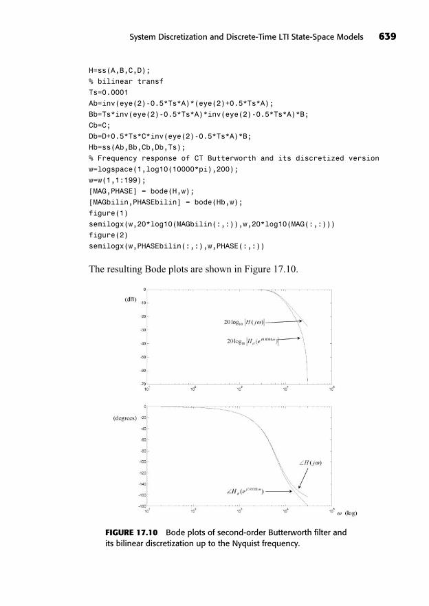
H=ss(A,B,C,D);
% bilinear transf
Ts=0.0001
Ab=inv(eye(2)-0.5*Ts*A)*(eye(2)+0.5*Ts*A);
Bb=Ts*inv(eye(2)-0.5*Ts*A)*inv(eye(2)-0.5*Ts*A)*B;
Cb=C;
Db=D+0.5*Ts*C*inv(eye(2)-0.5*Ts*A)*B;
Hb=ss(Ab,Bb,Cb,Db,Ts);
% Frequency response of CT Butterworth and its discretized version
w=logspace(1,log10(10000*pi),200);
w=w(1,1:199);
[MAG,PHASE] = bode(H,w);
[MAGbilin,PHASEbilin] = bode(Hb,w);
figure(1)
semilogx(w,20*log10(MAGbilin(:,:)),w,20*log10(MAG(:,:)))
figure(2)
semilogx(w,PHASEbilin(:,:),w,PHASE(:,:))
The resulting Bode plots are shown in Figure 17.10.
System Discretization and Discrete-Time LTI State-Space Models 639
FIGURE 17.10 Bode plots of second-order Butterworth filter and its bilinear discretization up to the Nyquist frequency.

640 Fundamentals of Signals and Systems
The filter can be implemented as a second-order recursive difference equation:
(c) Compute and plot on the same graph the first 30 points of the step responseof the Butterworth filter and its discretized version.
Answer: The following MATLAB script (last part of discretized.m, run afterthe script given in (b)) computes the continuous-time step response using the lsimcommand (which internally uses a c2d discretization) with a sampling period 10times shorter than Ts.
% Step responses
figure(3)
t=[0:0.00001:.00299]; % time vector to plot step resp of CT system
[y,ts,x]=lsim(H,ones(1,300),t);
plot(ts,y)
hold on
[yb,tsb,xb]=lsim(Hb,ones(1,30));
plot(tsb,yb,'o')
hold off
The resulting plot is shown in Figure 17.11.
y n y n y n x n[ ] . [ ] . [ ] . [ ]= + +1 1683 1 0 4241 2 0 06396 00 1279 1 0 06396 2. [ ] . [ ].x n x n+
FIGURE 17.11 Step responses of second-order Butterworth filter and its bilinear discretization.
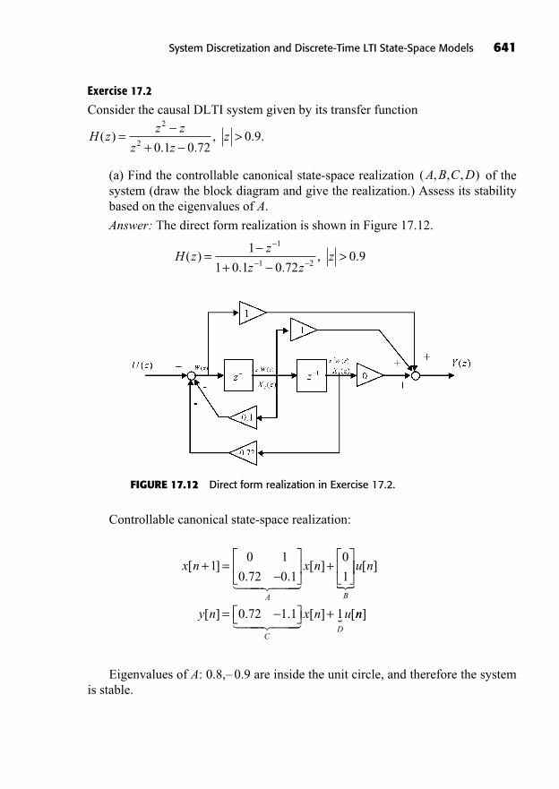
Exercise 17.2
Consider the causal DLTI system given by its transfer function
(a) Find the controllable canonical state-space realization of thesystem (draw the block diagram and give the realization.) Assess its stabilitybased on the eigenvalues of A.
Answer: The direct form realization is shown in Figure 17.12.
Controllable canonical state-space realization:
Eigenvalues of A: 0.8,– 0.9 are inside the unit circle, and therefore the systemis stable.
x n x n
A
[ ]. .
[ ]+ = +10 1
0 72 0 1
0
1� ��� ���
= +B
CD
u n
y n x n u
�
� ��� ��� �
[ ]
[ ] . . [ ] [0 72 1 1 1 nn]
H zz
z zz( )
. ., .=
+>1
1 0 1 0 720 9
1
1 2
( , , , )A B C D
H zz z
z zz( )
. ., . .=
+>
2
2 0 1 0 720 9
System Discretization and Discrete-Time LTI State-Space Models 641
FIGURE 17.12 Direct form realization in Exercise 17.2.
642 Fundamentals of Signals and Systems
(b) Compute the impulse response of the system h[n] by diagonalizing the Amatrix.
Answer: The impulse response of the system h[n] is given by
Exercises
Exercise 17.3
The causal continuous-time LTI system with transfer function is
discretized with a sampling period of for simulation purposes. Use the
c2d transformation first to get then the bilinear transformation to get
Answer:
Exercise 17.4
The causal continuous-time LTI system with transfer function
is discretized with a sampling period of for simulation purposes. The c2d transformation will be used first, and then it will be compared to the bilineartransformation.
(a) Find a continuous-time state-space realization of the system.
Ts = 0 1. s
ss s( )( )+ +1 2
G s( ) =
G zbilin ( ).G zc d2 ( ),
Ts = 0 01. s
s. +1
0 1 1G s( ) =
h n CA Bq n D nn[ ] [ ] [ ]
. ..
= +
=
1 1
0 72 1 10 1
0 72 00 1
0
11
0 72 1 1
1
.[ ] [ ]
. .
+
=
n
q n n
0.7809 0.7433
0.6247 0.6690
0 8 0
0 0 9
.
.
0.7809 0.7433
0.6247 0.6690
1
+
=
n
q n n
1
0
11
0 72 1 1
[ ] [ ]
. .0.77809 0.7433
0.6247 0.6690
0 8 0
0 0 9
1.
( .
n
))n 1
0.7809 0.7433
0.6247 0.6690+
=
10
11
0 0941 0 8
q n n[ ] [ ]
[ . .(( ) ( ) +n n
q n n1 1
1 0059 0 9 1. . ] [ ] [ ].
(b) Compute the discrete-time state-space system for
G(s) and its associated transfer function specifying its ROC.(c) Compute the discrete-time state-space system representing the bilinear
transformation of G(s), and its associated transfer
function specifying its ROC.
(d) Use MATLAB to plot the frequency responses
up to frequency on the same graph, where is the continuous-timefrequency. Use a decibel scale for the magnitude and a log frequency scalefor both magnitude and phase plots. Discuss any difference you observe.
Exercise 17.5
Consider the causal DLTI system specified by its transfer function:
(a) Find the controllable canonical state-space realization of thesystem. Assess its stability based on the eigenvalues of A.
(b) Compute the zero-input response of the system for the initial state
by diagonalizing the A matrix.
Answer:
Exercise 17.6
Consider the causal DLTI system with transfer function
(a) Find the observable canonical state-space realization of thesystem. Assess its stability based on the eigenvalues of A.
(b) Compute the zero-input response of the system for the initial state
1
1x[ ]0 =
y nzi[ ]
( , , , )A B C D
z, . .> 0 8z
z
.
.
+ 0 5
0 642H z( ) =
1
0x[ ]0 =
y nzi[ ]
( , , , )A B C D
H zz z
z zz( )
., .=
+>
2
2 0 5
1
2
s
2
G j G e G ebilinj T
c dj Ts s( ), ( ), ( )2
G zbilin ( ),( , , , )A B C Dbilin bilin bilin bilin
G zc d2 ( ),
( , , , )A B C Dc d c d c d c d2 2 2 2
System Discretization and Discrete-Time LTI State-Space Models 643
644 Fundamentals of Signals and Systems
Exercise 17.7
Find the controllable canonical state-space realization of the causal LTI system defined by the difference equation andcompute its transfer function from the state-space model, specifying its ROC.
Answer:
Exercise 17.8
The causal continuous-time LTI system with transfer function is
discretized with sampling period for simulation purposes. The c2dtransformation is used first, and then it is compared to the bilinear transformation.
(a) Find a state-space realization of
(b) Compute the discrete-time state-space system for G(s) using c2d and its as-sociated transfer function specifying its ROC.
(c) Find the bilinear transformation of G(s), specifying its ROC.Compute the difference between the two frequency responses obtained with c2d and the bilinear transformation; that is, compute
Evaluate this difference at DC and at thehighest discrete-time frequency.E e G e G ej
bilinj
c dj( ) : ( ) ( ).= 2
G zbilin ( )
G zc d2 ( ),
s, Re{ } .> 1ss++
21
G s( ) =
Ts = 0 1. s
ss++
21
G s( ) =
y n y n x n x n[ ] . [ ] [ ] . [ ]=0 4 1 2 0 4 1
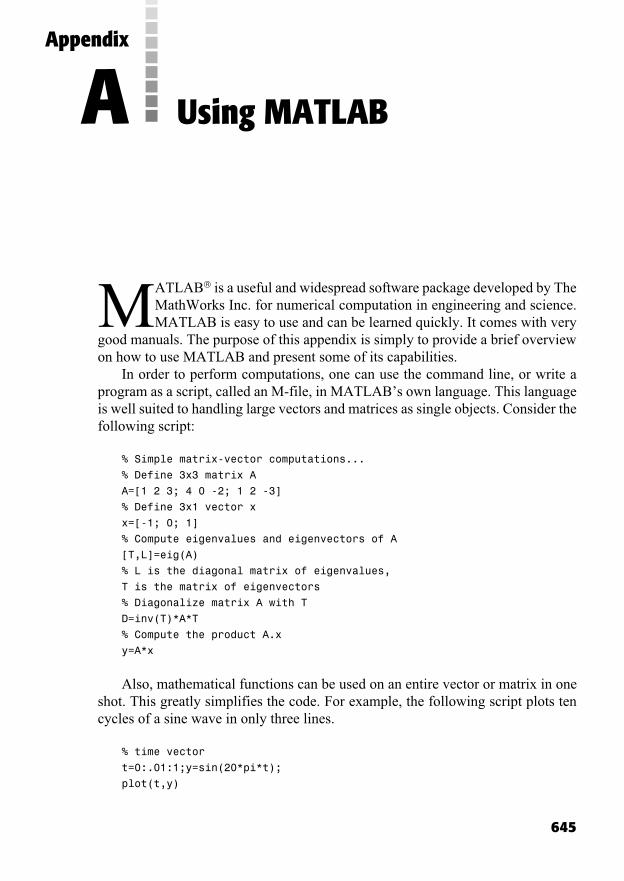
645
MATLAB® is a useful and widespread software package developed by TheMathWorks Inc. for numerical computation in engineering and science.MATLAB is easy to use and can be learned quickly. It comes with very
good manuals. The purpose of this appendix is simply to provide a brief overviewon how to use MATLAB and present some of its capabilities.
In order to perform computations, one can use the command line, or write aprogram as a script, called an M-file, in MATLAB’s own language. This languageis well suited to handling large vectors and matrices as single objects. Consider thefollowing script:
% Simple matrix-vector computations...
% Define 3x3 matrix A
A=[1 2 3; 4 0 -2; 1 2 -3]
% Define 3x1 vector x
x=[-1; 0; 1]
% Compute eigenvalues and eigenvectors of A
[T,L]=eig(A)
% L is the diagonal matrix of eigenvalues,
T is the matrix of eigenvectors
% Diagonalize matrix A with T
D=inv(T)*A*T
% Compute the product A.x
y=A*x
Also, mathematical functions can be used on an entire vector or matrix in oneshot. This greatly simplifies the code. For example, the following script plots tencycles of a sine wave in only three lines.
% time vector
t=0:.01:1;y=sin(20*pi*t);
plot(t,y)
Using MATLAB
Appendix
A
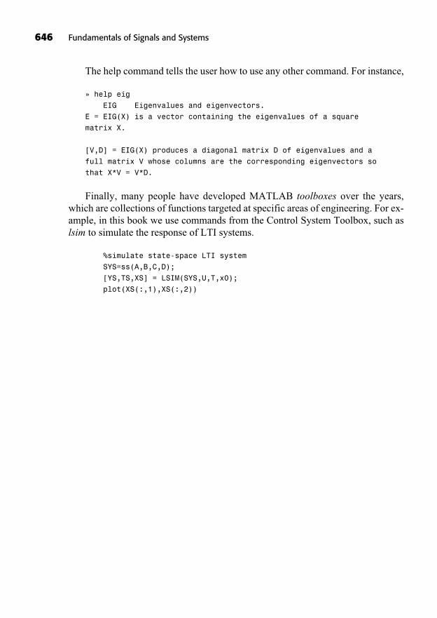
The help command tells the user how to use any other command. For instance,
» help eig
EIG Eigenvalues and eigenvectors.
E = EIG(X) is a vector containing the eigenvalues of a square
matrix X.
[V,D] = EIG(X) produces a diagonal matrix D of eigenvalues and a
full matrix V whose columns are the corresponding eigenvectors so
that X*V = V*D.
Finally, many people have developed MATLAB toolboxes over the years,which are collections of functions targeted at specific areas of engineering. For ex-ample, in this book we use commands from the Control System Toolbox, such aslsim to simulate the response of LTI systems.
%simulate state-space LTI system
SYS=ss(A,B,C,D);
[YS,TS,XS] = LSIM(SYS,U,T,x0);
plot(XS(:,1),XS(:,2))
646 Fundamentals of Signals and Systems
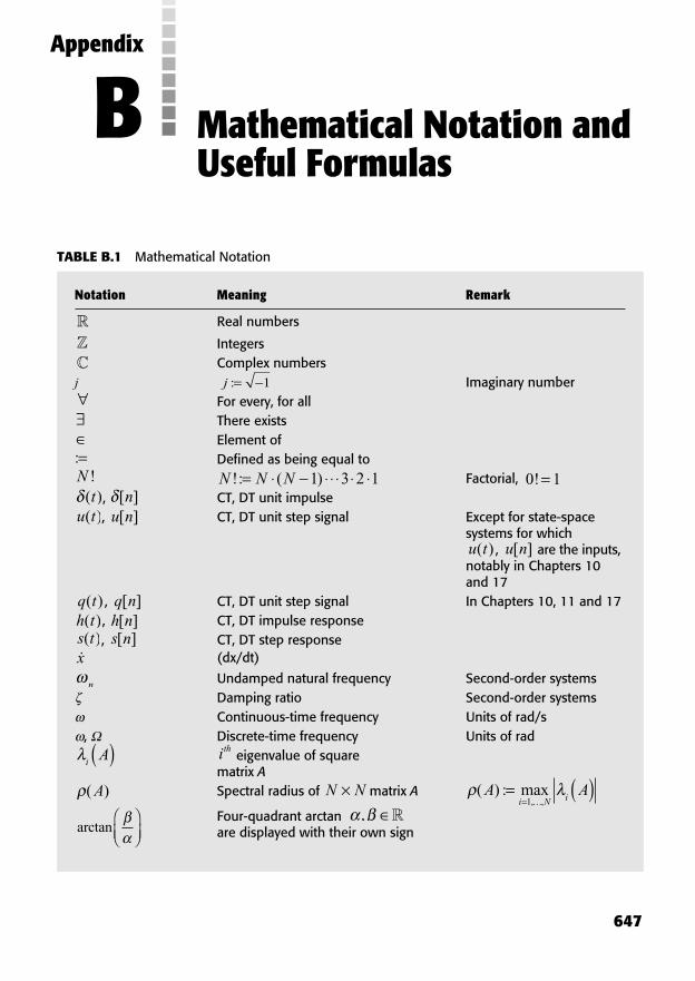
Notation Meaning Remark
Real numbers
IntegersComplex numbers
j Imaginary numberFor every, for allThere existsElement ofDefined as being equal to
Factorial,, CT, DT unit impulse, CT, DT unit step signal Except for state-space
systems for which , are the inputs,
notably in Chapters 10 and 17
, CT, DT unit step signal In Chapters 10, 11 and 17, CT, DT impulse response, CT, DT step response
(dx/dt)
Undamped natural frequency Second-order systemsDamping ratio Second-order systemsContinuous-time frequency Units of rad/s
, Discrete-time frequency Units of radeigenvalue of square
matrix ASpectral radius of matrix A
Four-quadrant arctan are displayed with their own sign
, �arctan
( ) : max, ,
A Ai N i
= ( )=1…
N N×( )A
ith
iA( )
n
�xs n[ ]s t( )h n[ ]h t( )q n[ ]q t( )
u n[ ]u t( )
u n[ ]u t( )[ ]n( )t
0 1!=N N N!: ( )= 1 3 2 1N !:=
j := 1
���
647
Mathematical Notation andUseful Formulas
Appendix
BTABLE B.1 Mathematical Notation
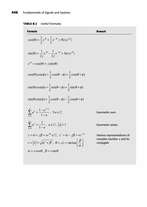
648 Fundamentals of Signals and Systems
Formula Remark
Geometric sum
Geometric series
z j re z j re
r z
j j
z
= + = = =
= + = ==
�,
, a2 2 rrctan
cos , sin= =r r
aa
a ak
k=
+
= <0
1
11, ,�
aa
aak
k
N N
=
+
=0
11
1, �
sin( )sin( ) cos( ) cos( )= +1
2
1
2
sin( )cos( ) sin( ) sin( )= + +1
2
1
2
cos( )cos( ) cos( ) cos( )= + +1
2
1
2
e jj = +cos( ) sin( )
sin( ) Im{ }= =1
2
1
2je
je ej j j
cos( ) Re{ }= + =1
2
1
2e e ej j j
TABLE B.2 Useful Formulas
Various representations ofcomplex number z and itsconjugate
649
CD-ROM FOLDERS
Applets: The Learnware applets
Chapter folders: Solutions to selected problems, MATLAB scripts, and all ofthe figures from the book, organized by chapter
Sample exams: Sample midterm and final examinations
The companion CD-ROM to the textbook contains files for
Solutions to odd-numbered problems in each chapter plus sample exams inPDF format
The detailed solutions to odd-numbered problems at the end of Chapter k {1,2,...,17}, are given in the file D:\Chapterk\Chapterkproblems.pdf, whereD: is assumed to be the CD-ROM drive. The sample midterm tests and finalexams are located in D:\Sample Exams\Covering Chapters 1 to 9, and D:\Sample Exams\Covering Chapters 10 to 17. All of the figures from each chap-ter can be found as TIFF files in D:\Chapterk\Figures.Learnware applets (discrete-time convolution, Fourier series, Bode plot)
The discrete-time convolution Java applet allows the user to enter the val-ues of an input signal and an impulse response and to visualize the convolutioneither as a sum of scaled and time-shifted impulse responses or as the sum ofthe values of a signal that is the product of the input signal and the time-re-versed and shifted impulses response. The convolution applet can be run bypointing a Java-enabled browser to
D:\Applets\Convolution\SignalGraph\Convolution.html.
The Fourier series Java applet uses an intuitive graphical user interface.One period of a periodic signal can be drawn using a mouse or a touchpad, andthe applet computes the Fourier series coefficients and displays a truncated
About the CD-ROM
Appendix
C

sum as an approximation to the signal at hand. The convolution applet can berun by pointing a Java-enabled browser to
D:\Applets\FourierSeries\FourierApplet.html.
The Bode applet is a Windows executable (.exe) file and can be found atD:\Applets\BodePlot\Bode.exe. Just double-click on it and you will be able tobuild a transfer function by dragging poles and zeros onto a pole-zero plot.Add a value for the DC gain of the overall transfer function and you will getthe Bode plot showing the actual frequency response of the system togetherwith its broken line approximation discussed in the text.MATLAB M-files of selected examples in the text.
These MATLAB script files, called M-files (with a .m extension) containsequences of MATLAB commands that perform a desired computation for anexample. The selected M-files are located in the Chapterk folders.
SYSTEM REQUIREMENTS
Minimum: Pentium II PC running Microsoft Windows 98. Microsoft InternetExplorer 5 or Netscape 7 browser with Java Plug-in 1.4 (www.sun.com). Ac-robat Reader 5 (www.adobe.com). MATLAB 5.3 with Control System Tool-box (www.mathworks.com).
Recommended: Pentium 4 PC running Microsoft Windows XP or Windows2000. Microsoft Internet Explorer 6 or Netscape 7 browser with Java Plug-in1.4 (www.sun.com). Acrobat Reader 5 (www.adobe.com). MATLAB 6.5 withControl System toolbox (www.mathworks.com).
650 Fundamentals of Signals and Systems
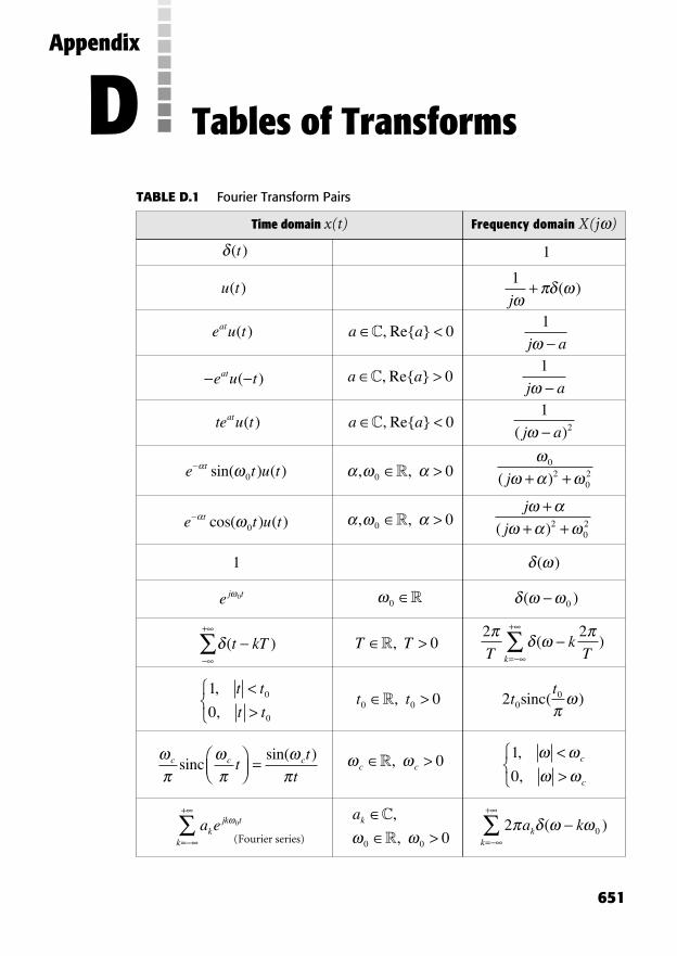
( )t 1
u t( )1
j+ ( )
e u tat ( ) a a <C, Re{ } 01
j a
e u tat ( ) a a >C, Re{ } 01
j a
te u tat ( ) a a <C, Re{ } 01
2( )j a
e t u tt sin( ) ( )0 , ,0 0>�0
202( )j + +
e t u tt cos( ) ( )0, ,0 0>�
j
j
++ +( )2
02
1 ( )
e j t00 � ( )0
( )t kT+
T T >�, 02 2
TkTk
( )=
+
1
00
0
,
,
t t
t t
<>
t t0 0 0>�, 2 00tt
sinc( )
c c ctt
tsinc =
sin( )c c >�, 0 1
0
,
,
<>
c
c
a ekjk t
k
0
=
+ ak>
��,
,0 0 02 0a kk
k
( )=
+
651
Tables of Transforms
Appendix
DTime domain x(t) Frequency domain X(j )
TABLE D.1 Fourier Transform Pairs
(Fourier series)
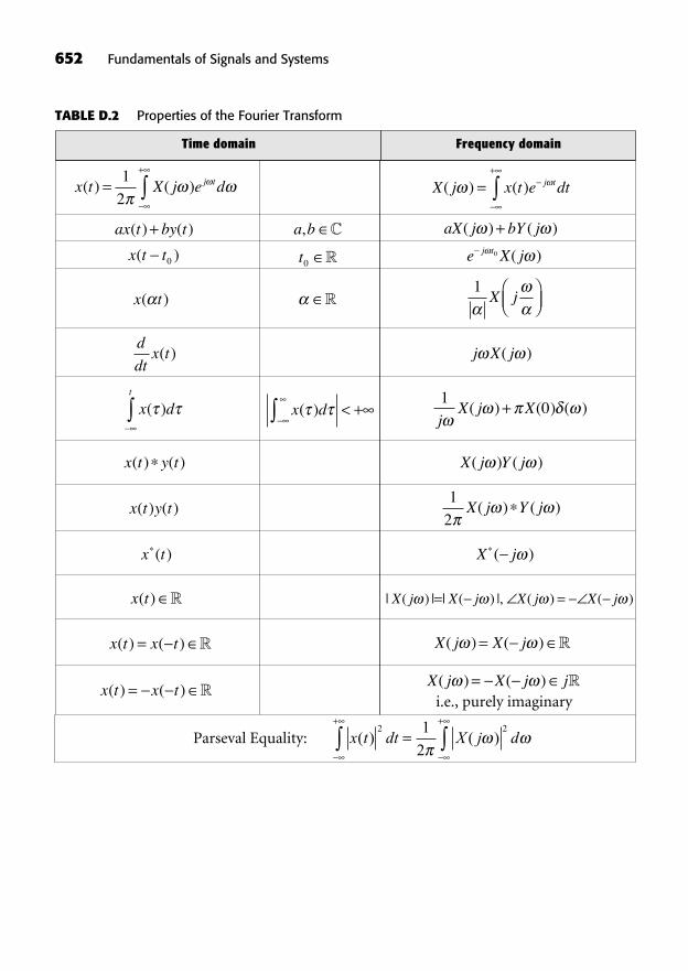
Time domain Frequency domain
652 Fundamentals of Signals and Systems
x t X j e dj t( ) ( )=+1
2X j x t e dtj t( ) ( )=
+
ax t by t( ) ( )+ a b, � aX j bY j( ) ( )+
x t t( )0 t0 � e X jj t0 ( )
x t( ) �1X j
d
dtx t( ) j X j( )
x dt
( ) x d( ) < +1
0j
X j X( ) ( ) ( )+
x t y t( ) ( ) X j Y j( ) ( )
x t y t( ) ( )1
2X j Y j( ) ( )
x t( ) X j( )
x t( ) � | ( ) | | ( ) |, ( ) ( )X j X j X j X j= =
x t x t( ) ( )= � X j X j( ) ( )= �
x t x t( ) ( )= � X j X j j( ) ( )= �
x t dt X j d( ) ( )2 21
2
+ +
=Parseval Equality:
i.e., purely imaginary
TABLE D.2 Properties of the Fourier Transform
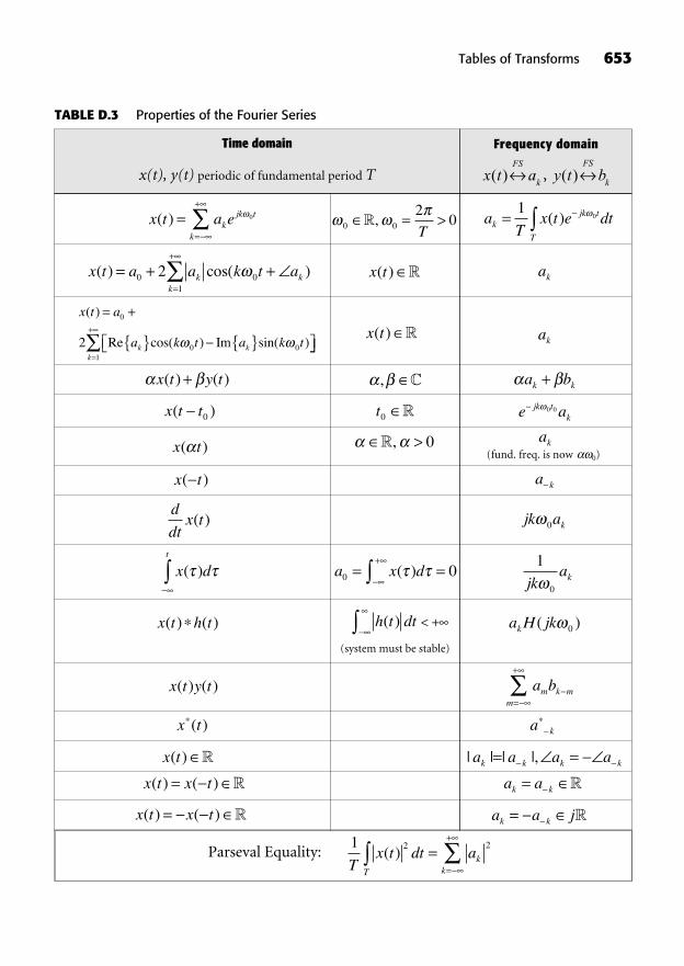
Tables of Transforms 653
TABLE D.3 Properties of the Fourier Series
Time domain
x(t), y(t) periodic of fundamental period T
Frequency domain
1 2 2
Tx t dt a
T
kk
( ) ==
+
x t aFS
k( ) y t b
FS
k( ),
x t a ekjk t
k
( ) ==
+0
0 0
20= >�,
Ta
Tx t e dtk
jk t
T
=1
0( )
x t a a k t ak kk
( ) cos( )= + +=
+
0 01
2 x t( ) � ak
x t a
a k t a k tk k
( )
Re cos( ) Im sin( )
= +
{ } { }0
0 02=
+
k 1
x t( ) � ak
x t y t( ) ( )+ , � a bk k+
x t t( )0 t0 � e ajk tk
0 0
x t( ) >�, 0 ak
x t( ) a k
d
dtx t( ) jk ak0
x dt
( ) a x d0 0= =+
( )1
0jkak
x t h t( ) ( ) h t dt( ) < + a H jkk ( )0
x t y t( ) ( ) a bm k mm=
+
x t( ) a k
x t( ) � | | | |,a a a ak k k k= =
x t x t( ) ( )= � a ak k= �
x t x t( ) ( )= � a a jk k= �
(fund. freq. is now 0)
(system must be stable)
Parseval Equality:
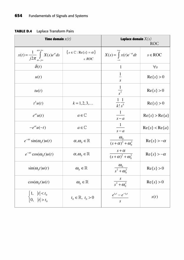
654 Fundamentals of Signals and Systems
Time domain x(t) Laplace domain X(s)ROC
x tj
X s e dsst
j
j
( ) ( )=+1
2
s s
ROC
={ }� : Re{ }X s x t e dtst( ) ( )=
+
s ROC
( )t 1 s
u t( )1
sRe{ }s > 0
tu t( )12s
Re{ }s > 0
t u tk ( ) k = 1 2 3, , ,…1 1
k sk!Re{ }s > 0
e u tat ( ) a C 1
s aRe{ } Re{ }s a>
e u tat ( ) a C 1
s aRe{ } Re{ }s a<
e t u tt sin( ) ( )0 , 0 � 02
02( )s + + Re{ }s >
e t u tt cos( ) ( )0 , 0 �s
s
++ +( )2
02 Re{ }s >
sin( ) ( )0t u t 0 � 02
02s + Re{ }s > 0
cos( ) ( )0t u t 0 �s
s202+ Re{ }s > 0
1
00
0
,
,
t t
t t
<> t t0 0 0>�,
e e
s
t s t s0 0
x t( )
TABLE D.4 Laplace Transform Pairs
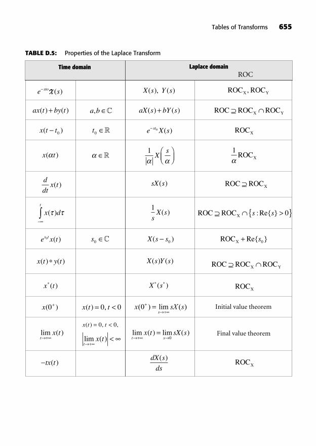
Tables of Transforms 655
TABLE D.5: Properties of the Laplace Transform
e sstoX ( ) X s Y s( ), ( ) ROC ROCX Y,
ax t by t( ) ( )+ a b, � aX s bY s( ) ( )+ ROC ROC ROCX Y
x t t( )0 t0 � e X sst0 ( ) ROCX
x t( ) �1X
s 1ROCX
d
dtx t( ) sX s( ) ROC ROCX
x dt
( )1
sX s( ) ROC ROCX >{ }s s:Re{ } 0
e x ts t0 ( ) s0 � X s s( )0 ROC Re{X 0+ s }
x t y t( ) ( ) X s Y s( ) ( ) ROC ROC ROCX Y
x t( ) X s( ) ROCX
x( )0+ x t t( ) ,= <0 0 x sX ss
( ) lim ( )0+
+=
lim ( )t
x t+
x t t
tx t
( ) , ,
lim ( )
= <
+<
0 0lim ( ) lim ( )t s
x t sX s+
=0
tx t( )dX s
ds
( )ROCX
Final value theorem
Initial value theorem
Time domain Laplace domain ROC
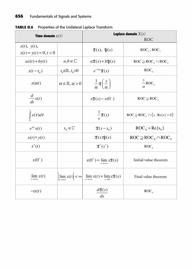
x t y t
x t y t t
( ), ( ),
( ) ( ) ,= = <0 0X Y( ), ( )s s ROC ROC
X Y,
ax t by t( ) ( )+ a b, � a s b sX Y( ) ( )+ ROC ROC ROCX Y
x t t( )0 t t0 0 0>�, e sstoX ( ) ROCX
x t( ) >�, 01
Xs 1
ROCX
d
dtx t( ) s s xX ( ) ( )0 ROC ROC
X
x dt
( )0
1
ssX ( ) ROC ROC
X>{ }s s: Re{ } 0
e x ts t0 ( ) s0 � X ( )s s0 ROC Re{sX 0+ }
x t y t( ) ( ) X Y( ) ( )s s ROC ROC ROCX Y
x t( ) X ( )s ROCX
x( )0+ x s ss
( ) lim ( )0+
+= X
lim ( )t
x t+
lim ( )t
x t+
< lim ( ) lim ( )t s
x t s s+
=0
X
tx t( ) d s
ds
X ( ) ROCX
656 Fundamentals of Signals and Systems
TABLE D.6 Properties of the Unilateral Laplace Transform
Final value theorem
Initial value theorem
Time domain x(t) Laplace domain X(s)ROC

Tables of Transforms 657
TABLE D.7 Discrete-Time Fourier Transform Pairs
Time domain x[n] Frequency domain X(e j )always periodic of period 2
x n X e e dj j n[ ] ( )=1
2 2
X e x n ej j n
n
( ) [ ]==
+
[ ]n 1
[ ]n n0 n0 � e j n0
u n[ ]1
12+
=
+
ekj
k
( )
1 2 2( )=
+
kk
u n n u n n[ ] [ ]+ 0 0 1 n n0 0 0>�,sin ( )
sin( )
n0 1 2
2
+
a u nn [ ] a a <C, 11
1 ae j
( ) [ ]n a u nn+1 a a <C, 11
1 2( )ae j
a u nn [ ]1 a a >C, 11
1 ae j
r n u nn cos( ) [ ]0 r r, ,0 0>�1
1 20
02 2+
r e
r e r e
j
j j
cos( )
cos( )
r n u nn sin( ) [ ]0 r r, ,0 0>�r e
r e r e
j
j j
sin( )
cos( )0
02 21 2 +
cos( )0n 0 � ( ) ( )+ +=
+
0 02 2k kk
sin( )0n 0 � j k kk
+ +=
+
( ) ( )0 02 2
sin c c cn
n
n= sinc
c
c< <�,
01 2
0
, ,
,
k kc �otherwise
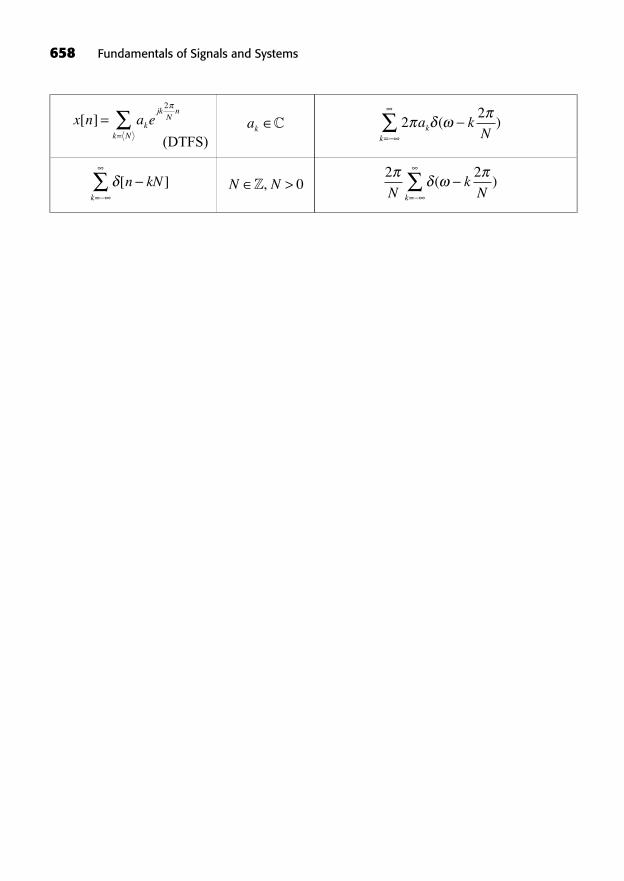
658 Fundamentals of Signals and Systems
x n a ekjkNn
k N
[ ] ==
2
ak � 22
a kNk
k
( )=
[ ]n kNk=
N N >�, 02 2
NkNk
( )=
(DTFS)
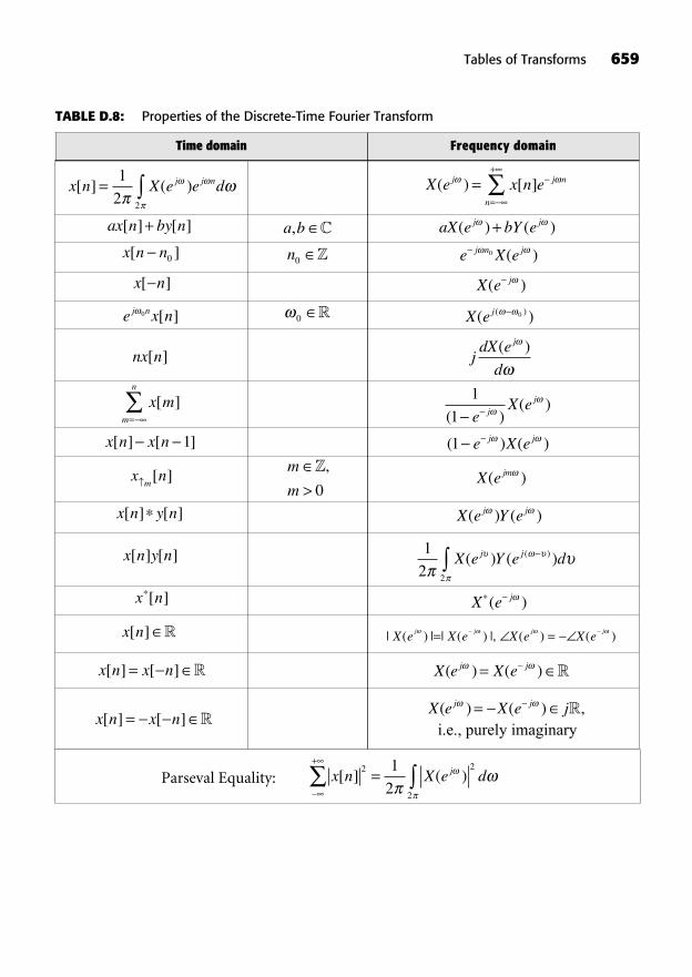
Tables of Transforms 659
Time domain Frequency domain
TABLE D.8: Properties of the Discrete-Time Fourier Transform
x n X e e dj j n[ ] ( )=1
2 2
X e x n ej j n
n
( ) [ ]==
+
ax n by n[ ] [ ]+ a b, � aX e bY ej j( ) ( )+x n n[ ]0 n0 � e X ej n j0 ( )
x n[ ] X e j( )
e x nj n0 [ ] 0 � X ej( )( )0
nx n[ ] jdX e
d
j( )
x mm
n
[ ]=
1
1( )( )
eX ej
j
x n x n[ ] [ ]1 ( ) ( )1 e X ej j
x nm[ ]
m
m >�,
0X ejm( )
x n y n[ ] [ ] X e Y ej j( ) ( )
x n y n[ ] [ ] 1
2 2
X e Y e dj j( ) ( )( )
x n[ ] X e j( )
x n[ ] � | ( ) | | ( ) |, ( ) ( )X e X e X e X ej j j j= =
x n x n[ ] [ ]= � X e X ej j( ) ( )= �
x n x n[ ] [ ]= �X e X e jj j( ) ( ) ,= �
x n X e dj[ ] ( )2 2
2
1
2
+
=Parseval Equality:
i.e., purely imaginary
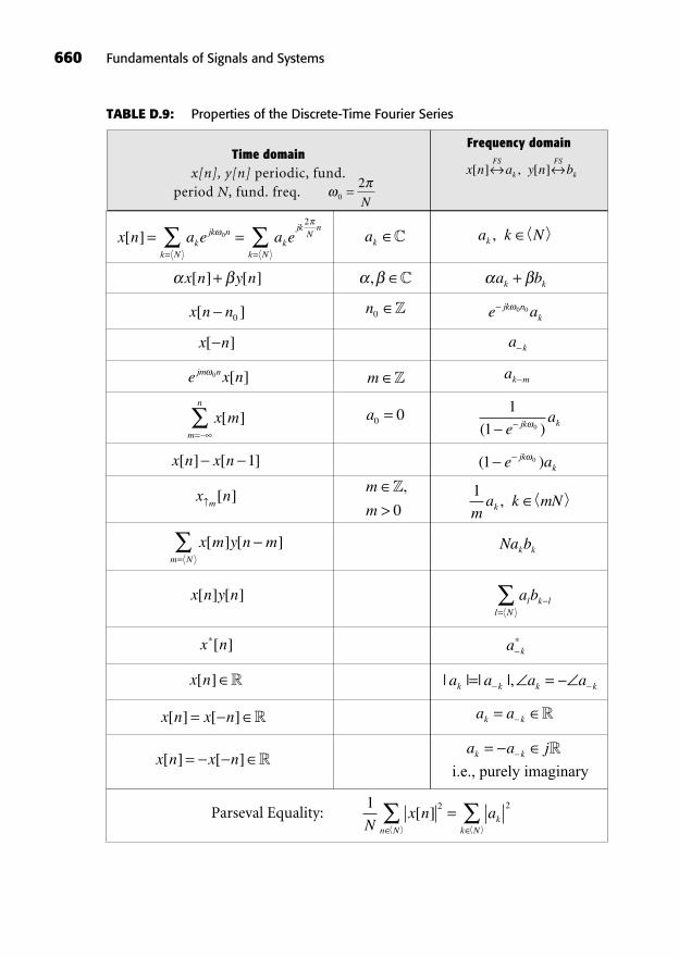
660 Fundamentals of Signals and Systems
Time domainx[n], y[n] periodic, fund.
period N, fund. freq.
Frequency domain
TABLE D.9: Properties of the Discrete-Time Fourier Series
0
2=N
x n a y n bFS
k
FS
k[ ] , [ ]
x n a e a ekjk n
k Nk
jkNn
k N
[ ] = == =
0
2
ak � a k Nk ,
x n y n[ ] [ ]+ , � a bk k+
x n n[ ]0n0 � e ajk n
k0 0
x n[ ] a k
e x njm n0 [ ] m � ak m
x mm
n
[ ]=
a0 0= 1
1 0( )eajk k
x n x n[ ] [ ]1 ( )1 0e ajkk
x nm[ ]
m
m >�,
01
ma k mNk ,
x m y n mm N
[ ] [ ]=
Na bk k
x n y n[ ] [ ] a bl k ll N=
x n[ ] a k
x n[ ] � | | | |,a a a ak k k k= =
x n x n[ ] [ ]= � a ak k= �
x n x n[ ] [ ]= �a a jk k= �
1 2 2
Nx n a
n Nk
k N
[ ] =Parseval Equality:
i.e., purely imaginary
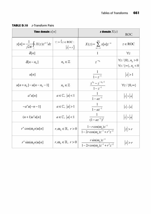
Tables of Transforms 661
TABLE D.10 z-Transform Pairs
Time domain x[n] z domain X(z)ROC
x nj
X z z dzn[ ] ( )=1
21
C�
C : :=
=
{
}z
z r
ROCX z x n z n
n
( ) [ ]==
+
z ROC
[ ]n 1 z
[ ]n n0 n0 � z n0 ><
z n
z n
/ { },
/{ },
0 0
00
0
u n[ ]1
1 1zz >1
u n n u n n[ ] [ ]+ 0 0 1 n0 � z z
z
n n0 0 1
11z / { , }0
a u nn [ ] a a <C, 11
1 1azz a>
a u nn [ ]1 a a >C, 11
1 1azz a<
( ) [ ]n a u nn+1 a a <C, 11
1 1 2( )azz a>
r n u nn cos( ) [ ]0 r r, ,0 0>� 1
1 20
1
01 2 2+
r z
r z r z
cos( )
cos( )z r>
r n u nn sin( ) [ ]0 r r, ,0 0>� r z
r z r z
sin( )
cos( )0
1
01 2 21 2 +
z r>
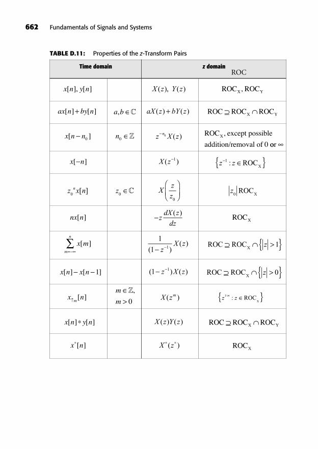
662 Fundamentals of Signals and Systems
TABLE D.11: Properties of the z-Transform Pairs
Time domain z domainROC
x n y n[ ], [ ] X z Y z( ), ( ) ROC ROCX Y,
ax n by n[ ] [ ]+ a b, � aX z bY z( ) ( )+ ROC ROC ROCX Y
x n n[ ]0 n0 � z X zn0 ( ) ROC , except possible
addition/removal of 0 X
oor
x n[ ] X z( )1z z{ }1 : ROC
X
z x nn0
[ ] z0� X
z
z0
z0
ROCX
nx n[ ] zdX z
dz
( )ROCX
x mm
n
[ ]=
1
1 1( )( )
zX z ROC ROC
X>{ }z 1
x n x n[ ] [ ]1 ( ) ( )1 1z X z ROC ROCX
>{ }z 0
x nm[ ]
m
m >�,
0 X zm( ) z zm1/ :{ }ROCX
x n y n[ ] [ ] X z Y z( ) ( ) ROC ROC ROCX Y
x n[ ] X z( ) ROCX
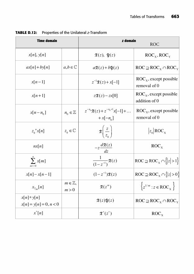
Tables of Transforms 663
TABLE D.12: Properties of the Unilateral z-Transform
Time domain z domainROC
x n y n[ ], [ ] X Y( ), ( )z z ROC ROCX Y,
ax n by n[ ] [ ]+ a b, � a z b zX Y( ) ( )+ ROC ROC ROCX Y
x n[ ]1 z z x+1 1X ( ) [ ]ROC , except possible
removal of 0X
x n[ ]+1 z z zxX ( ) [ ]0 ROC , except possible
addition of 0X
x n n[ ]0 n0 � z z z x
x n
n n ++ ++
0 0 1
0
1X ( ) [ ]
[ ]
… ROC , except possible
removal of 0X
z x nn0
[ ] z0� X
z
z0
z0
ROCX
nx n[ ] zd z
dz
X ( ) ROCX
x mm
n
[ ]= 0
1
1 1( )( )
zzX ROC ROC
X>{ }z 1
x n x n[ ] [ ]1 ( ) ( )1 1z zX ROC ROCX >{ }z 0
x nm[ ]
m
m >�,
0X ( )zm z zm1/ :{ }ROC
X
x n y n
x n y n n
[ ] [ ]
[ ] [ ] ,= = <0 0X Y( ) ( )z z ROC ROC ROCX Y
x n[ ] X ( )z ROCX

This page intentionally left blank
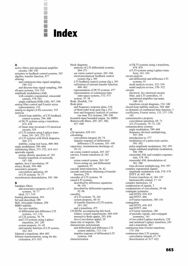
665
Index
Aactive filters and operational amplifier
circuits, 340–343actuators in feedback control systems, 383algebra, transfer function, 477aliasing
and continuous-time signal sampling,549–552
and discrete-time signal sampling, 560all-pass systems, 316–319amplitude modulation (AM)
with complex exponential, sinusoidalcarriers, 578–581
single-sideband (SSB-AM), 587–590analog filter control and Fourier series
representation, 132analog-to-digital (A/D) converter, 555analysis
closed-loop stability, of LTI feedbackcontrol systems, 394–400
of DLTI systems using z-transform,474–478
of linear time-invariant LTI electricalcircuits, 329
of LTI systems using Laplace trans-form, 241–243, 272–273
of LTI systems with block diagrams,264–271
stability, using root locus, 400–404angle modulation, 599–604antialiasing filters, 551–552, 614–615aperiodic signals
energy-density spectrum of, 183Fourier transform of sawtooth,
187–188applets, Java Convolution, 59arrays, Routh, 399–400associative property
convolution operation, 69of LTI systems, 76–77
asynchronous demodulation, 583–586
Bbandpass filters
and associative property of LTIsystems, 76–77
ideal, 517–519beating phenomenon, 583bel unit described, 290Bell, Alexander Graham, 290BIBO stability
See also stabilityof differential and difference LTI
systems, 112–116of LTI systems, 78–79and LTI systems using Laplace
transform, 241–243system property, 41–42and transfer function of LTI system,
262–263bilateral z-transform, 484–485bilinear transformation, using for dis-
cretization, 631–635
block diagramsanalysis of LTI differential systems,
264–271car cruise control system, 265–266electromechanical feedback control
system (fig.), 385LTI feedback control system (fig.), 383realization of rational transfer function,
480–483representation of DLTI systems, 477representation of continuous-time
state-space systems, 372–373system, 35–38
Bode, Hendrik, 316Bode plots
and frequency response plots, 219of third-order loop gain (fig.), 412time and frequency analysis of continu-
ous time TLI systems, 290–296bounded-input bounded-output. See BIBOButterworth filters, 205–207, 306,
637–640
Cc2d operator, 628–631calculating
convolution integral, 69–74impulse response of differential,
difference LTI systems, 101–109capacitors, instantaneous discharge of,
30–32car cruise control system, 265–267carriers, Fourier transform of, 182cars
cruise control system, 265–267forces acting on, and differential
equations, 93cascade interconnection, 36, 42cascade realization, obtaining of transfer
function, 270cascades of LTI systems, 76causal LTI systems
described by difference equations,96–101
described by differential equations,92–96
causalityof LTI systems, 78, 241system property, 40–41of transfer function of LTI system,
261–262and z-transform, 475
CD-ROM, accompanying this bookfolders, system requirements, 649–650interactive Bode applet, 293, 650Java Convolution applet, 59
chain rule of impulse, 106characteristic polynomials
and differential and difference LTIsystem stability, 112–116
impulse response of differential LTIsystems, 104
characterization
of DLTI systems using z-transform,474–478
of LTI systems using Laplace trans-form, 241–243
circuit analysisand differential and difference LTI
systems, 91mesh analysis review, 332–334nodal analysis review, 330–332
circuitselectrical. See electrical circuitsfilter, and LTI controllers, 53operational amplifier (op-amp),
340–343transform circuit diagrams, 334–340
closed-loop stability analysis, 394–400co-domains of continuous-time function, 3coefficients, Fourier series, 135, 137–139,
142communicative property
convolution operation, 69, 71of LTI systems, 74–75, 120
communication systemsangle modulation, 599–604frequency-division multiplexing,
597–599introduction to, 577modulation of a pulse-train carrier,
591–592pulse-amplitude modulation, 592–595single-sideband amplitude modulation,
586–590sinusoidal AM, and complex exponen-
tials, 578–581sinusoidal AM, demodulation of,
581–586time-division multiplexing, 595–597
complex exponential signalsamplitude modulation with, 578–579DTFT of, 445–446Fourier transform of, 184–187harmonically related, 17–18
complex harmonics, 18compression of signals, 5computations of convolution, 59–66conjugate symmetry
and DTFS, 434–435and DTFT, 444of Fourier transform, 180–181
conjugationand DTFS, 434–435and DTFT, 444of Fourier transform, 180of periodic signals, and conjugate
symmetry, 141of two-sided Laplace transform, 238and unilateral Laplace transform, 245and z-transform, 467
continuous-time Fourier transform,175–184
continuous-time LTI systemsconvolution integral, 67–74discretization of, 617–622
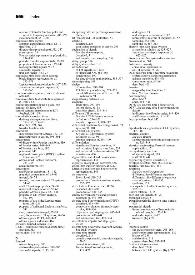
relation of transfer function poles andzeros to frequency response, 286–290
state models of, 351–360continuous-time signals
complex exponential signals, 12–17described, 2–3discrete-time processing of, 552–557even signals, 23Fourier series representation pf periodic,
134–137periodic complex exponentials, 17–19properties of Fourier series, 139–141real exponential signals, 9–12sinusoidal signals, 19unit step signal (fig.), 27
continuous-time state-space systemsblock diagram representation of,
372–373Laplace transform solution for, 367–370zero-state, zero-input response of,
361–366continuous-time systems, discretization of,
628–636continuous-time to discrete-time operator
(CT/DT), 553contour integration in the z-plane, 468contour, Nyquist, 405control systems, introduction to LTI
feedback, 381–394controllable canonical form
deriving state-space model from,352–355, 618–621
described, 271, 269transfer function, 482
controllersin feedback control systems, 382–383naive approach to design, 393–394
convergenceof discrete-time Fourier transform, 439of Fourier series, 141–148of Fourier transform, 192pointwise, 147region of convergence (ROC), Laplace
transform, 225of two-sided Laplace transform,
234–235and z-transform, 464
convolutionand Fourier transform, 181–182graphical computation of, 59–62integral, 69–74integral, continuous-time LTI systems,
54–66and LTI system properties, 74–80numerical computation of, 62–66periodic, of two signals, 433–434property in LTI system analysis,
192–199property of two-sided Laplace trans-
form, 238–239property of unilateral Laplace transform,
245sum, convolution integral, 62–69sum, discrete-time LTI systems, 54–66of two signals, DTFT, 442–443of two signals, z-domain, 466
critically damped systems, 302CT/DT (continuous-time to discrete-time)
operator, 553cycles, duty, 143–144
Ddamped
natural frequency, 312and overdamped systems, 302–305sinusoidal signals, 13–15, 187
dampening ratio vs. percentage overshoot(table), 313
DC motors and LTI controllers, 53decibels
described, 290gain values expressed in (table), 291
decimation of signalsSee also downsamplingdescribed, 5and impulse train sampling, 559
delay, group, 316delay systems, ideal, 315demodulation
of FM signals, 601–604of sinusoidal AM, 581–586synchronous, 590for time-division multiplexing, 595–597
demultiplexing, 598design
of controllers, 393–394FIR filters by windowing, 527–531use of differential and difference LTI
systems in, 91diagonalizing matrixes, 361diagrams
Bode plots, 290–296system block, 35–38transform circuit, 334–340
difference LTI systemsSee also LTI difference systemsdefinition of, 96–101impulse response of, 109–112
differential equations describing casual LTIsystems, 91–101
differential LTI systemsSee also LTI differential systemsdefinition of, 92–96impulse response of, 101–109
differentiationsignals, and Fourier transform, 181and two-sided Laplace transform, 239and unilateral Laplace transform, 247in z-domain, 466
digital filter control and Fourier seriesrepresentation, 132
digital-to-analog (D/A) converter, 556direct form transfer function, 269, 271Dirichlet conditions and Fourier series
representation, 146discrete-time
filters, ideal, 510–519processing of continuous-time signals,
552–557discrete-time Fourier series (DTFS)
described, 425–430properties of, 430–435
duality between analysis and syntheticequations of, 449–450
discrete-time Fourier transform (DTFT)described, 435–439geometric evaluation from pole-zero
plot, 498–504of periodic, and step signals, 445–449properties of, 439–444and z-transform, 460, 497–504
discrete-time impulse and step signals,25–26
discrete-time linear time-invariant systems.See DLTI systems
discrete-time signalsdescribed, 2–3complex exponential, sinusoidal signals,
20–21convolution between, 66Fourier transforms of aperiodic,
435–439
odd signals, 23real, complex exponential, 9–17representing in terms of impulses, 54–57sampling, 542–546sampling of, 557–563
discrete-time state-space systemsz-transform solution of, 625–627zero-state, zero-input responses of,
622–625discretization. See system discretizationdiscriminators, 601distributive property
convolution operation, 69of LTI systems, 75–76
DLTI (discrete-time linear time-invariant)systems analysis and characterizationusing z-transform, 474–478convolution sum, 54–66described, 426
domainsmapped by time functions, 3time. See time domain
downsamplingdescribed, 5and DTFT, 441
DTFS. See discrete-time Fourier seriesDTFT. See discrete-time Fourier transform
dualityin discrete-time Fourier series, 449–450and Fourier transform, 191–192
duty cycle described, 143
Eeigenfunctions, eigenvalues of LTI systems,
117–118electrical circuits
See also circuitsLaplace transform technique application
to, 329–343electrical engineering, Parseval theorem
applicability, 151energy-density spectrum
of aperiodic signal, 183and DTFT, 444
engineering systems described, 2envelope detectors, 584, 586, 598, 607equality, Parseval, 150–151equations
See also specific equationsdifference. See difference equationsdifferential. See differential equationsstate, of systems, 351–352synthesis, 135
error signals in feedback control systems,382–383
Euler’s relation, 13, 15even and odd signals, 23–25expanded signals, 5expanding periodic discrete-time signals,
425exponential signals
linear combinations of harmonicallyrelated complex, 132–134
real and complex, 9–17truncated (fig.), 27
Ffeedback control
car cruise control system, 265–266and Fourier series representation, 132history of, 381and rise time, 311systems described, 382–383
feedback interconnectiondescribed, 37–38between two LTI systems (fig.), 217
666 Index
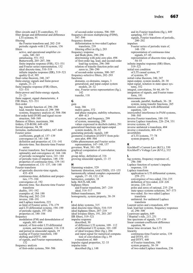
filter circuits and LTI controllers, 53filter design and differential and difference
LTI systems, 91filtering
the Fourier transform and, 202–210periodic signals with LTI system, 156
filtersactive, and operational amplifier cir-
cuits, 340–343antialiasing, 551–552Butterworth, 205–207, 306finite-impulse response (FIR), 521–531and Fourier series representation, 132ideal discrete-time, 510–519infinite impulse response (IIR), 519–521quality Q of, 305
final-value theorem, 240, 247finite-energy signals and finite-power
signals, 21–23finite-impulse response (FIR) filters,
521–531finite-power and finite-energy signals,
21–23finite support, signal characteristic, 4FIR filters, 521–531first-order
lag, transfer function of, 296–298lead, transfer function of, 298–300systems, frequency analysis of, 504–506
first-order hold (FOH) and signal recon-struction, 548–549
flatness of filters, maximum, 306folders, CD-ROM, 649–650forced response, 94, 98formulas, mathematical (table), 647–648Fourier series
coefficients, graph of, 137–139convergence of, 141–148definition and properties of, 131–141discrete-time. See discrete-time Fourier
seriesFourier transform. See Fourier transformoptimality and convergence of, 144–146of periodic rectangular wave, 141–144of periodic train of impulses, 148–150properties of continuous-time, 139–141representation of, 131–137, 146–148
Fourier transformof aperiodic discrete-time signals,
435–439continuous-time, definition and proper-
ties, 175–184convergence of, 192discrete-time. See discrete-time Fourier
transformduality, 191–192examples of, 184–188filtering and, 202–210inverse, 188–191and Laplace transform, 223as limit of Fourier series, 176–179and LTI differential systems, 194–199of periodic signals, 197–202properties of, 180–184
frequencymodulation (FM) and demodulation of
signals, 601–604natural, of first-order LTI differential
system, and time constant, 116–118and period in sinusoidal signals, 19scaling of Fourier transform, 180shifting and DTFT, 440of signals, and Fourier representation,
132frequency analysis
of first-order systems, 504–506
of second-order systems, 506–509frequency-division multiplexing (FDM),
597–599frequency domain
differentiation in two-sided Laplacetransform, 239
filtering effect in (fig.), 203frequency response
and Bode plots, 290–296determining with pole-zero plot, 498of first-order lag, lead, and second-order
lead-lag systems, 296–300relation of transfer function poles and
zeros to, 286–290of second-order systems, 300–307
frequency-selective filters, 202–203functions
domains, co-domains, ranges, 3generalized, and input-output system
models, 26–32sinc, Fourier series representation (fig.),
142transfer, 118
Ggain
loop, 386matrix gains, 372and phase margins, stability robustness,
409–413of system, and frequency, 299of system, measuring, 290values expressed in decibels (table), 291
generalized functions and input-outputsystem models, 26–32
generating periodic signals, 149geometric evaluation of DTFT from pole-
zero plot, 498–504Gibbs phenomenon and Fourier series
representation, 147–148, 157governor, Watt, 381–382graphical computation of convolution,
59–62group delay, definition of, 316growing sinusoidal signals, 13–15
HHamming window, 529harmonic distortion, total (THD), 153–155harmonically related complex exponential
signals, 17–18, 132–134harmonics, complex, 18help, MATLAB, 646highpass filters
and Fourier transform, 207– 210ideal, 514–517
Hilbert transformers, 589homogeneity, system property, 38–39
Iideal delay systems, 315ideal discrete-time filters, 510–519ideal highpass filters, 207–210ideal lowpass filters, 191, 203–207IIR filters, 519–521impulse response
described, 30of difference LTI systems, 109– 112of differential LTI system, 101–109of ideal lowpass filter (fig.), 204and input signal for numerical computa-
tion of convolution (fig.), 59z-transform of, 460
impulse signal properties, 32–33impulse train
described (fig.), 148
and its Fourier transform (fig.), 449sampling, 557–558signals, Fourier transform of periodic,
200–202impulses
Fourier series of periodic train of,148–150
representation of continuous-timesignals, 67–68
representation of discrete-time signals,54–55
infinite impulse response (IIR) filters,519–521
initial rest conditionof LTI casual system, 97of systems, 95
initial-value theorem, 240, 247input-output, system models, 26–38input signal, notation in state-space sys-
tems, 352integral, convolution, 54–66, 69–74integration of signals, and Fourier trans-
form, 181interconnection
cascade, parallel, feedback, 36– 38system, using transfer functions, 265
interest, calculating with differentialequation, 128
intersymbol interference in PAM systems,594–595
inverse Fourier transform, 188–191inverse Laplace transform, 226–234, 331inverse systems, 42inverse unilateral z-transform, 484inverse z-transform, 468–474invertibility
of LTI systems, 77–78system property, 42
KKirchhoff’s Current Law (KCL), 330Kirchhoff’s Voltage Law (KVL), 332
Llag systems, frequency responses of,
296–300Laplace function of system’s impulse
response, 118Laplace transform
application to LTI differential systems,259–271
convergence of two-sided, 234–235definition of two-sided, 224–226inverse, 226–234poles and zeros of rational, 235–236state-space systems solutions, 367–373two-sided. See two-sided Laplace
transformunilateral. See unilateral Laplace
transformLaurent series and z-transform, 459lead, lead-last systems, frequency responses
of, 296–300Learnware applets, 649l’Hopital’s rule, 215, 251line spectrum of signals, 137–139linear constant-coefficient difference
equation, 96linear time-invariant. See LTIlinearity
continuous-time Fourier series, 139and DTFS, 431and DTFT, 440of Fourier transform, 180system property, 38–39of two-sided Laplace transform, 236
Index 667

of unilateral Laplace transform, 244and z-transform, 465
logarithmic scale and Bode plots, 290loop gain described, 386lowpass filters, 169–171
and Fourier transform, 203–207ideal, 191, 510–514second-order RLC, 301
LTI (linear time-invariant) systemsanalysis and characterization using
Laplace transform, 241–243continuous-time. See continuous-time
LTI systemsconvolution property in, 192–199convolution sum, 53–62described, 1, 91–96difference. See difference LTI systemsdifferential. See differential LTI systemsdiscrete-time, convolution sum, 54–66eigenfunctions, eigenvalues, 117–118exponential signals, 9–17frequency response of, 132invertibility of, 77–78modeling physical processes with, 53multivariable, 373properties of, 74–80response to periodic input, 155–157Routh’s stability criterion, 398–400steady-state response to periodic signals,
155–157transfer function of, 260–264without memory, 77
LTI difference systemsSee also difference LTI systemsstate models of, 617–622transfer function characterization of,
478–480LTI differential systems
See also differential LTI systemsanalysis with initial conditions using
unilateral Laplace transform,272–273
application of Laplace transform to,259–271
BIBO stability of, 113–114Fourier transform and, 194–199time constant and natural frequency of
first-order, 116–118transient and steady-state responses of,
274–276LTI feedback control systems
closed-loop stability analysis, 394–400introduction to, 381–394stability analysis using root locus,
400–404
MM-files, 645mass-spring-damper system, 301, 322–325mathematical notation, formulas (table),
647–648MathWorks Inc., 645MATLAB software package, using,
645–646maximum flatness of filters, 306mechanical mass-spring-damper system,
301memory
LTI systems without, 77and memoryless systems, 40
mesh analysisof circuits, 332–334transform circuit for, 338–340
minimal state-space realizations, 369models
input-output system, 26–38signal, 1–11state. See state modelssystem. See system models
modulationangle, 599–604pulse-amplitude (PAM), 592–595of pulse-train carrier, 591–592
motors, DC, and LTI controllers, 53moving-average filters, 522–524multiplexing
frequency-division (FDM), 597–599time-division, 595–597
multiplicationand convolution property, 182of two signals, 140–141of two signals, DTFS, 434of two signals, DTFT, 443
Nnodal analysis
of electrical circuits, 330–332transform circuit for, 334–338
noise and ideal discrete-time filters, 510non-minimum phase systems, 316–319noncausal systems, 41notation, mathematical (table), 647–648Nth harmonic components of signals, 133numerical computation of convolution,
62–66Nyquist criterion for stability analysis,
404–409
Oobservable canonical form
deriving state-space model from,621–622
deriving state-space system model from,355–357
odd and even signals, 23–25op-amp circuits, 340–343operational amplifier circuits, 340–343operators
c2d, 628–631CT/DT (continuous-time to discrete-
time), 553DT/CT (discrete-time to continuous-
time), 555–556optimality of Fourier series, 144–146orthogonal sets of signals, 18output disturbance, 383overdamped systems, 302overshoot of step response, 311–313
PPAM (pulse-amplitude modulation)
systems, 594–595parallel interconnection, 36–37Parseval equality
and DTFT, 444for Fourier transforms, 184
Parseval theorem and signal power,150–151, 162
partial fraction expansion, 228passband described, 202, 510period and frequency in sinusoidal signals,
19periodic
complex exponential and sinusoidalsignals, 17–21
input, LTI systems’ response to,155–157
rectangular waves, Fourier series of,141–144
periodic signals
classes with Fourier series representa-tion, 146
continuous-time, Fourier series repre-sentation of, 134–137
described, 8–9discrete-time (fig.), 435DTFT of, 445–449Fourier transform of, 197–202fundamental frequency of, 132power spectrum of, 151–152setup for generating (fig.), 149steady-state response of LTI system to,
155–157phase-lock loop (PLL), 601, 603phase
margins in stability analysis, 409–413plane, state trajectories and, 370–372systems, non-minimum, 316–319
PLL (phase-lock loop), 601, 603pointwise convergence, 147pole-zero plot
determining system’s frequency re-sponse with, 498
geometric evaluation of DTFT from,498–504
qualitative evaluation of frequencyresponse from, 285–290
of transfer function (fig.), 321of z-transform (fig.), 463, 468
polesand zeros of rational Laplace transforms,
235–236and zeros of transfer function, 260–261
polynomialscharacteristic, of LTI difference system,
114–116characteristic, of LTI differential
system, 112power engineering and Fourier series
representation, 132power series of z-transform, 473–474power spectrum of signals, 151–152Principle of Argument, 404–405Principle of Superposition
and linear discrete-time systems, 55and linear property of LTI systems, 68
process models and differential and differ-ence LTI systems, 91
propertiesbasic system, 38–42of continuous-time Fourier series,
139–141convolution, in LTI system analysis,
192–199of discrete-time Fourier series, 430–435of discrete-time Fourier transform,
439–444of Fourier series, 131–141of Fourier transform, 180–184of impulse signal, 32–33LTI systems, 74–80of two-sided Laplace transform,
236–240two-sided z-transform, 465–468of unilateral Laplace transform,
244–247unilateral z-transform, 484–485of z-transform, 465–468
pulse-amplitude modulation (PAM),592–595
pulse signalscontinuous-time rectangular (fig.), 28integration of rectangular, and step unit
(fig.), 29pulse-train carrier, modulation of, 591–592
668 Index
Qqualitative evaluation of fre-quency
response from pole-zero plot, 285–290
quality Q of filters, 305–306
Rrange of continuous-time function, 3rational transfer functions
block diagram realization of, 480–483LTI differential systems and, 259–264
RC circuitsfiltering periodic signal with, 156impulse response, step response (figs.),
80real discrete-time exponential signals, 10real exponential signals, 9–12realizations
of first-order lag (fig.), 298of LTI differential systems, 264obtaining of transfer function, 268–272
reconstructing signals, 546–549, 560–563rectangular waves
input to LTI system (fig.), 164periodic, Fourier series of, 141–144
reference signals in feedback controlsystems, 382–383
region of convergence (ROC)of inverse Laplace transform, 226–234of Laplace transform, 225of z-transform, 464–465, 474–476
regulators in feedback control systems,386–387
repeating signals. See periodic signalsrepresenting
continuous-time signals in terms ofimpulses, 67–68
discrete-time periodic signals withFourier series, 426–430
discrete-time signals in terms of im-pulses, 54–57
Fourier series, 131–132periodic signals using Fourier transform,
197–202resistance, finite-energy and finite-power
signals, 21–23resistances and impedances in Laplace
domain, 336resistor-inductor-capacitor. See RLC
circuitsresponses
forced, zero-state, 94frequency. See frequency responseimpulse. See impulse responsesteady-state, of LTI system to period
signal, 155–157step. See step responsezero-state, zero-input, 360–366
reversal, time, 6rise time of step response, 307–311RLC (resistor-inductor-capacitor) circuits,
deriving state-space representationsfrom, 357–360
robustness, stability, 409–413ROC. See region of convergenceroot locus and stability analysis, 400–404Routh, E.J., 398running sum of signals, 434
Ssampled-data systems, 552, 556sampling
aliasing and, 549–552described, 541
of discrete-time signals, 542–546,557–563
property, impulse signal, 32–33, 106sawtooth signals
in Fourier series representation, 136Fourier transform of aperiodic, 187–188line spectrum of (fig.), 138
scalingtime. See time scalingin z-domain, 465
second-order systemsfrequency analysis of, 506–509frequency response of, 300–307
sensitivity function and feedback controlsystems, 387–390
settling time of step response, 313–315shift, time, 7sidebands, AM, 587–590signal interpolation using perfect sinc
function, 547signal models, 1–11signal reconstruction, 546–549signals
See also specific signal typecontinuous-time, discrete-time, 2–3described, 1discrete-time impulse and step, 25–26even and odd, 23–25exponential, described, 9–17finite-energy, and finite-power, 21–23frequency spectrum of, 132function of time as, 2–4fundamental components of, 133impulse, 32–33and Laplace transform. See Laplace
transformlow-distortion transmission over com-
munication channel, 77orthogonal sets, 18periodic complex exponential and
sinusoidal, 17–21periodic, described, 8–9power spectrum of, 151–152satisfying Dirichlet conditions, 146sawtooth. See sawtooth signalssome useful, 12–26
sinc functionFourier series representation, 142perfect signal interpolation using, 547
single-sideband amplitude modulation(SSB-AM), 587–590
sinusoidal AMand AM radio, 586demodulation of, 581–586
sinusoidal signalsaliasing of (fig.), 550amplitude modulation with, 579–581complex exponentials, 20–21continuous-time, 19dampened, growing, 13–15and periodic complex exponential
signals, 17–21slowed down signals, 5spectral coefficients
and Fourier series representation, 135of impulse train (fig.), 149
spectrumenergy-density, of aperiodic signal, 183line, of signals, 137–139of signal and carrier (fig.), 182signal frequency, 132
sped up signals, 5square wave signal, continuous-time
periodic (fig.), 8
stabilitySee also BIBO stabilityclosed-loop analysis, 394–400for DLTI systems, 475–476Nyquist criterion, plot, 404– 409robustness, 409–413Routh’s criterion for, 398–400theorem, 369, 626using Fourier transform on LTI differen-
tial systems, 194stability analysis using root locus, 400–404stable LTI systems
step response of, 307–315time and frequency analysis of continu-
ous time, 285–290state models of continuous-time LTI
systems, 351–360state-space models
deriving with controllable canonicalform, 618–621
deriving with observable canonicalform, 621–622
state-space systems, Laplace transformsolution for continuous-time, 367–373
state trajectories and the phase plane, 370–372states in systems described, 351–352steady-state and transient response of LTI
differential systems, 274–276step-invariant transformation, using for
discretization, 628–636step response
impulse response obtained by differenti-ation of, 106–109
of stable LTI systems, 307–315of systems, 27unit, of LTI system, 79–80
step signalsand discrete-time impulse signals, 25–26DTFT of, 445–449
stopband described, 202, 510sum, convolution, 54–66superheterodyne receivers, 598–599,
612–613supernodes, 331, 337, 341superposition principle, 55suspension systems, 322, 323synchronous demodulation, 581–583, 590synthesis equation, 135system
step response of, 27term’s use in engineering, 2
system discretizationof continuous-time systems, 628–636described, 617–618using bilinear transformation, 631–635using step-invariant transformation,
628–631system models
basic system properties, 38–42input-output, 26–38, 35system block diagrams, 35–38
system requirements, CD-ROM, 650systems
See also specific systembasic properties, 38–42feedback control, described, 382–383first-order. See first-order systemsideal delay, 315initial rest state, 95linear time-invariant. See LTIPAM, 594–595sampled-data, 552, 556second-order. See second-order systemsstates in, 351–352
Index 669
TTHD (total harmonic distortion), 153–155time
constant of first-order LTI differentialsystem, and natural frequency,116–118
delay and unilateral Laplace transform,244–245
functions of, as signals, 2–4settling, vs. percentage overshoot
(table), 313time-division multiplexing, 595–597time domain
differentiation in two-sided Laplacetransform, 239
differentiation of unilateral Laplacetransform, 246
time expansion. See upsamplingtime invariance, system property, 39–40time reversal
in continuous-time Fourier series, 140and DTFS, 431and DTFT, 440functions for, 6and z-transform, 466
time scalingin continuous-time Fourier series, 140described, 4–6and DTFS, 431–433and DTFT, 441of Fourier transform, 180of impulse signal, 32–33of two-sided Laplace transform, 237and unilateral Laplace transform, 245
time-shifted impulsesin continuous-time Fourier series,
139–140in discrete-time signals, 54–77
time shiftingdescribed, 7and DTFS, 431and DTFT, 440of Fourier transform, 180of two-sided Laplace transform,
236–237and z-transform, 465
time variable, transformation of, 4–7total harmonic distortion (THD), 153–155tracking with unity feedback system, 385train, impulse (fig.), 148transfer function
algebra, and z-domain, 477Bode magnitude plots (fig.), 292, 295
Bode phase plots (fig.), 293, 295characterization of LTI difference
systems, 478–480of differential LTI system, 260–264of DLTI systems, 474first-order lag, 296–298ideal delay systems, 315of LTI systems, 118, 241Nyquist plot of, 406–409obtaining realizations of, 268– 272pole-zero plot of (fig.), 321poles and zeros, relation to frequency
response, 286– 290rational, and LTI differential systems,
259–264transform circuit
diagrams, 334–340for mesh analysis, 338–340for nodal analysis, 334–338
transformations of time variable, 4–7transforms
Fourier. See Fourier transformLaplace. See Laplace transformz-transform. See z-transform
transient and steady-state response of LTIdifferential systems, 274–276
transmissionin closed-loop transfer function, 386as complementary sensitivity function in
feedback system, 390–393Tustin’s method, 631two-sided Laplace transform
definition of, 224–226properties of, 236–240
two-sided z-transformdevelopment of, 460–465properties of, 465–468
Uunderdamped systems, 302unilateral Laplace transform
analysis of LTI differential systems withinitial conditions, 272–273
definition of, 243–244properties of, 244–247
unilateral z-transform, 483–486unit doublet described, 33–34unit impulse
described, 25generalized function definition, 28response of LTI system, 68–69signal (fig.), 30
unit doublet and higher derivatives,33–34
unit ramp signal, 27unit step response of LTI system, 79–80unity feedback systems
described, 385stability in, 394
upsamplingdescribed, 5, 432and DTFT, 441and z-transform, 466
VVandermonde matrix, 111variables, continuous vs. discrete, 2voltage, Kirchhoff’s Voltage Law (KVL),
332voltage controlled oscillator (VCO), 601
WWatt, James, 381waves, Fourier series of periodic rectangu-
lar, 141–144windowing, FIR filter design by, 527–531
Zz-transform
development of two-sided, 460–465discrete-time state-space systems
solution, 625–627and DTFT, relationship between,
497–504inverse, 468–474pole-zero plot (fig.), 463, 468properties of, 465–468of system’s impulse response, 118two-sided. See two-sided z-transformunilateral, 483–486
zero-input responsesdescribed, 273of discrete-time state-space systems,
622–625of continuous-time state-space systems,
360–366zero-order hold (ZOH) and signal recon-
struction, 547–548zero-state response, 94, 273, 360–366,
622–625zeros
and poles of rational Laplace transforms,235–236
and poles of transfer function, 260–261
670 Index