fundamentals of global climate change science erik ramberg temperature of the earth radiative...
TRANSCRIPT
Fundamentals of Global Climate Change Science
Erik Ramberg
• Temperature of the Earth• Radiative balance in the atmosphere• Forcings and the Ice Ages• Direct measurements of the surface temperature• Ice sheet melting• Ocean sea level rise and acidification• Predictions for the future

Radiative Balance on Earth
So – what temperature do we predict the Earth to have?
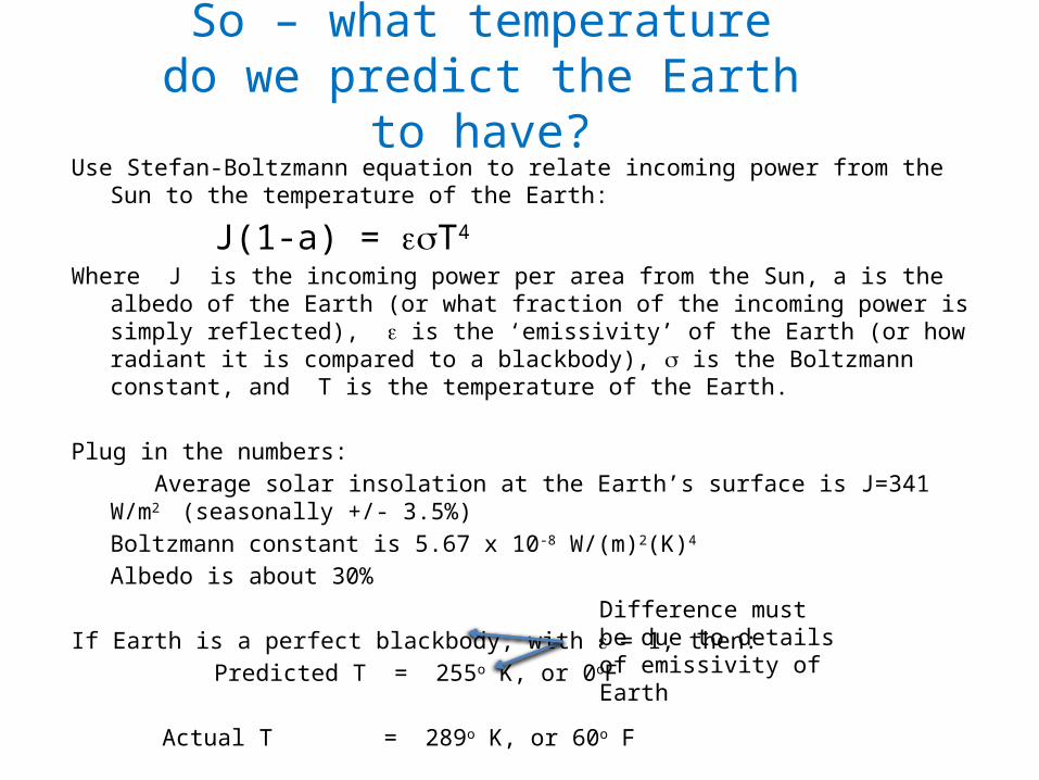
Use Stefan-Boltzmann equation to relate incoming power from the Sun to the temperature of the Earth:
J(1-a) = esT4
Where J is the incoming power per area from the Sun, a is the albedo of the Earth (or what fraction of the incoming power is simply reflected), e is the ‘emissivity’ of the Earth (or how radiant it is compared to a blackbody), s is the Boltzmann constant, and T is the temperature of the Earth.
Plug in the numbers: Average solar insolation at the Earth’s surface is J=341 W/m2 (seasonally +/- 3.5%)
Boltzmann constant is 5.67 x 10⁻⁸ W/(m)2(K)4
Albedo is about 30%
If Earth is a perfect blackbody, with e = 1, then: Predicted T = 255o K, or 0oF
Actual T = 289o K, or 60o F
Difference must be due to details of emissivity of Earth
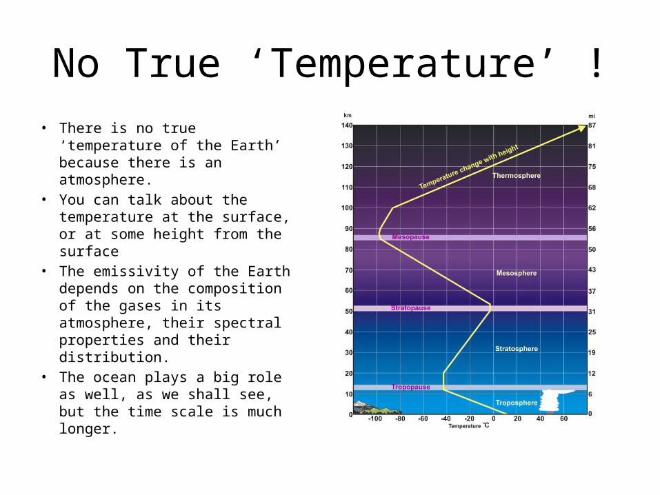
No True ‘Temperature’ !• There is no true ‘temperature
of the Earth’ because there is an atmosphere.
• You can talk about the temperature at the surface, or at some height from the surface
• The emissivity of the Earth depends on the composition of the gases in its atmosphere, their spectral properties and their distribution.
• The ocean plays a big role as well, as we shall see, but the time scale is much longer.
5
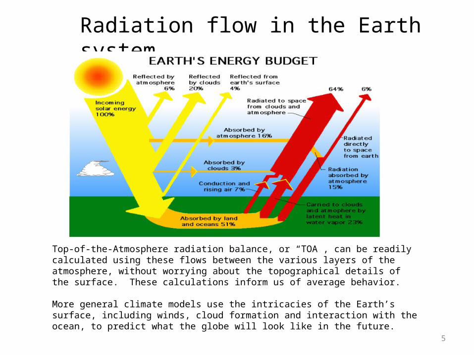
Radiation flow in the Earth system
Top-of-the-Atmosphere radiation balance, or “TOA”, can be readily calculated using these flows between the various layers of the atmosphere, without worrying about the topographical details of the surface. These calculations inform us of average behavior.
More general climate models use the intricacies of the Earth’s surface, including winds, cloud formation and interaction with the ocean, to predict what the globe will look like in the future.
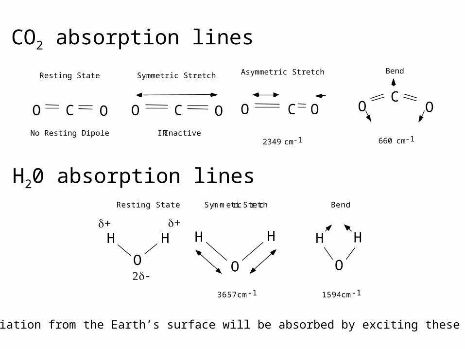
CO O
Symmetric Stretch Asymmetric Stretch Bend
CO OC
O OCO O
Resting State
No Resting Dipole IR Inactive2349 cm-1 660 cm-1
CO2 absorption lines
O
H H++
-
Resting State
O
H H
O
H H
Symmetric Stretch Bend
3657 cm-1 1594 cm-1
H20 absorption lines
Infrared radiation from the Earth’s surface will be absorbed by exciting these vibrations.
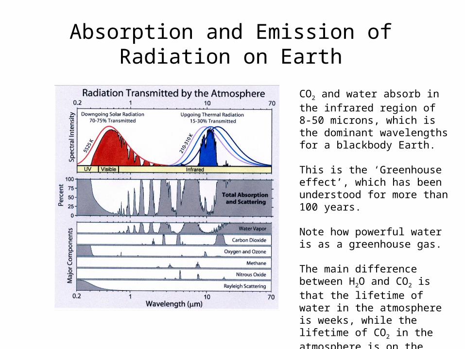
Absorption and Emission of Radiation on Earth
CO2 and water absorb in the infrared region of 8-50 microns, which is the dominant wavelengths for a blackbody Earth.
This is the ‘Greenhouse effect’, which has been understood for more than 100 years.
Note how powerful water is as a greenhouse gas.
The main difference between H2O and CO2 is that the lifetime of water in the atmosphere is weeks, while the lifetime of CO2 in the atmosphere is on the order of 1000 years.
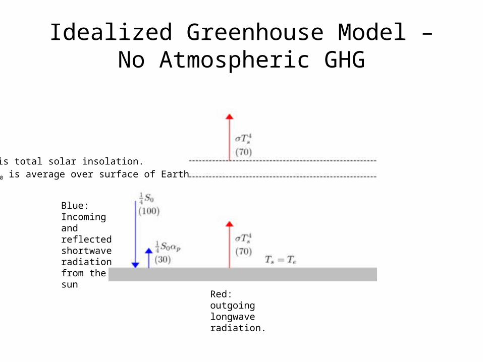
Idealized Greenhouse Model –No Atmospheric GHG
Blue: Incoming and reflected shortwave radiation from the sun
Red: outgoing longwave radiation.
S0 is total solar insolation.¼ S0 is average over surface of Earth
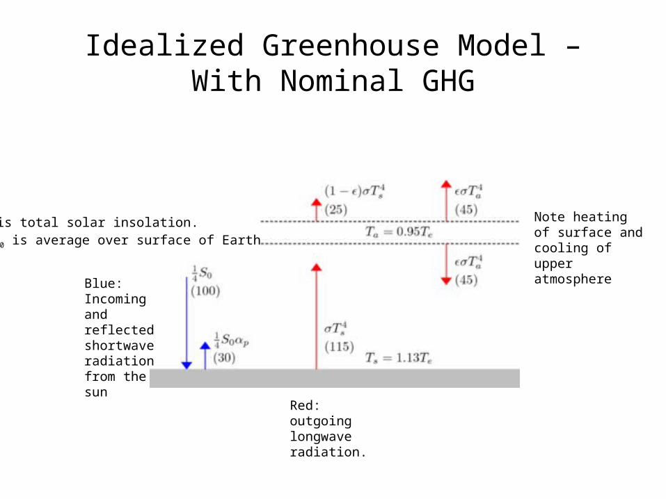
Idealized Greenhouse Model –With Nominal GHG
Red: outgoing longwave radiation.
Note heating of surface and cooling of upper atmosphere
Blue: Incoming and reflected shortwave radiation from the sun
S0 is total solar insolation.¼ S0 is average over surface of Earth
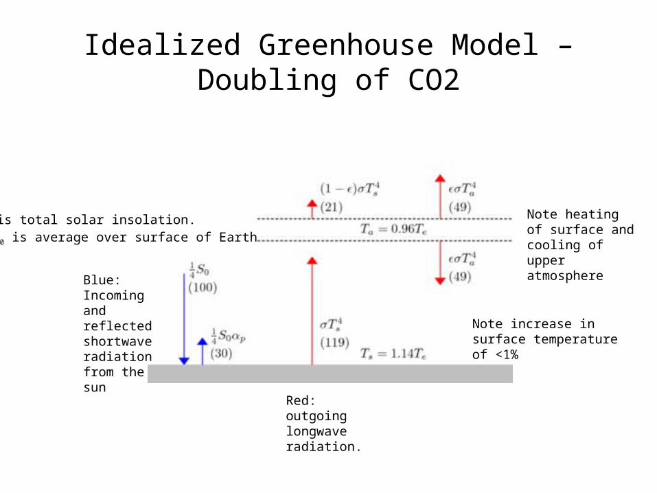
Idealized Greenhouse Model –Doubling of CO2
Red: outgoing longwave radiation.
Note heating of surface and cooling of upper atmosphere
Note increase in surface temperature of <1%
Blue: Incoming and reflected shortwave radiation from the sun
S0 is total solar insolation.¼ S0 is average over surface of Earth

Forcings
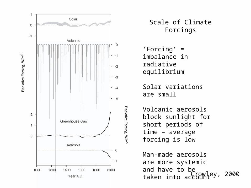
‘Forcing’ = imbalance in radiative equilibrium
Solar variations are small
Volcanic aerosols block sunlight for short periods of time – average forcing is low
Man-made aerosols are more systemic and have to be taken into account
Only greenhouse gasforcing looks like therecent temperature rise.
Scale of Climate Forcings
Crowley, 2000
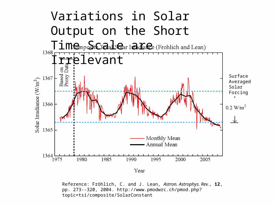
Reference: Fröhlich, C. and J. Lean, Astron. Astrophys. Rev., 12, pp. 273--320, 2004. http://www.pmodwrc.ch/pmod.php?topic=tsi/composite/SolarConstant
Variations in Solar Output on the Short Time Scale are Irrelevant
Surface Averaged Solar Forcing
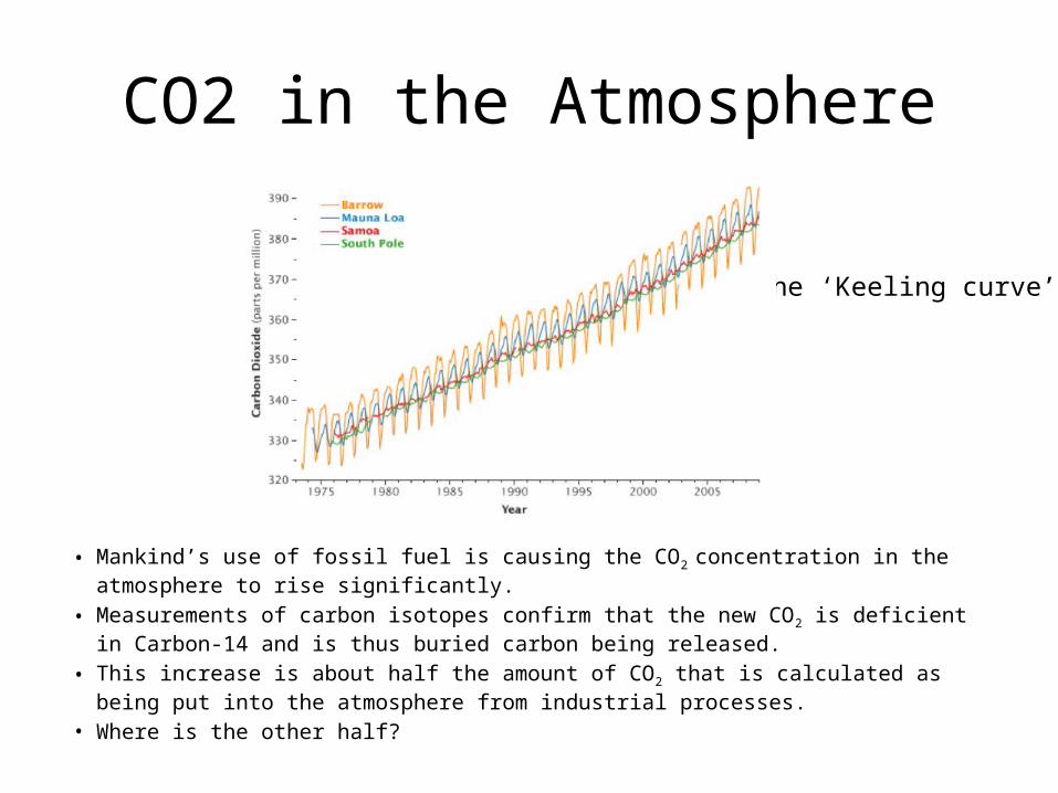
CO2 in the Atmosphere
• Mankind’s use of fossil fuel is causing the CO2 concentration in the atmosphere to rise significantly.
• Measurements of carbon isotopes confirm that the new CO2 is deficient in Carbon-14 and is thus buried carbon being released.
• This increase is about half the amount of CO2 that is calculated as being put into the atmosphere from industrial processes.
• Where is the other half?
The ‘Keeling curve’
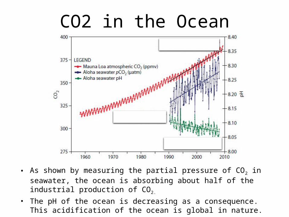
CO2 in the Ocean
• As shown by measuring the partial pressure of CO2 in seawater, the ocean is absorbing about half of the industrial production of CO2.
• The pH of the ocean is decreasing as a consequence. This acidification of the ocean is global in nature.
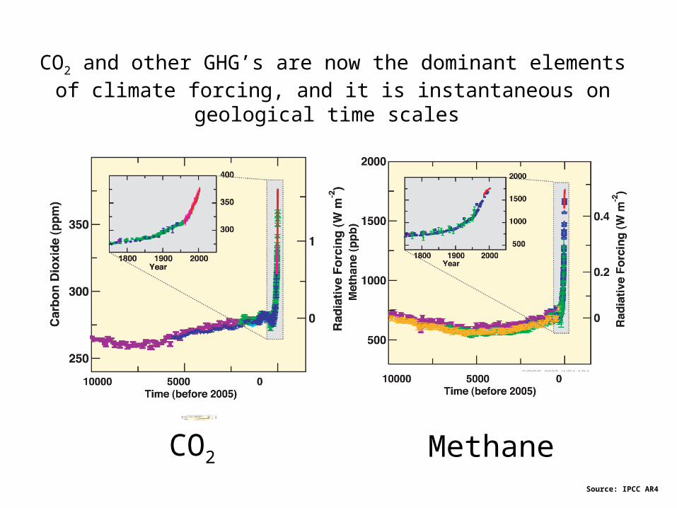
CO2 and other GHG’s are now the dominant elements of climate forcing, and it is instantaneous on geological time scales
Source: IPCC AR4
CO2 Methane
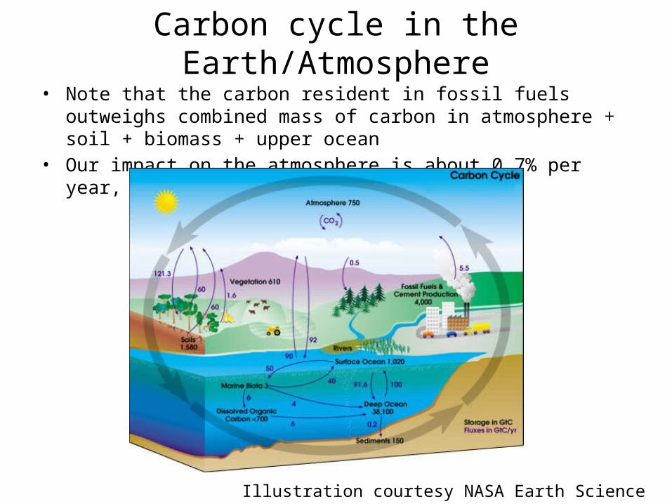
Carbon cycle in the Earth/Atmosphere• Note that the carbon resident in fossil fuels outweighs combined mass of
carbon in atmosphere + soil + biomass + upper ocean• Our impact on the atmosphere is about 0.7% per year, and rising
Illustration courtesy NASA Earth Science Enterprise.
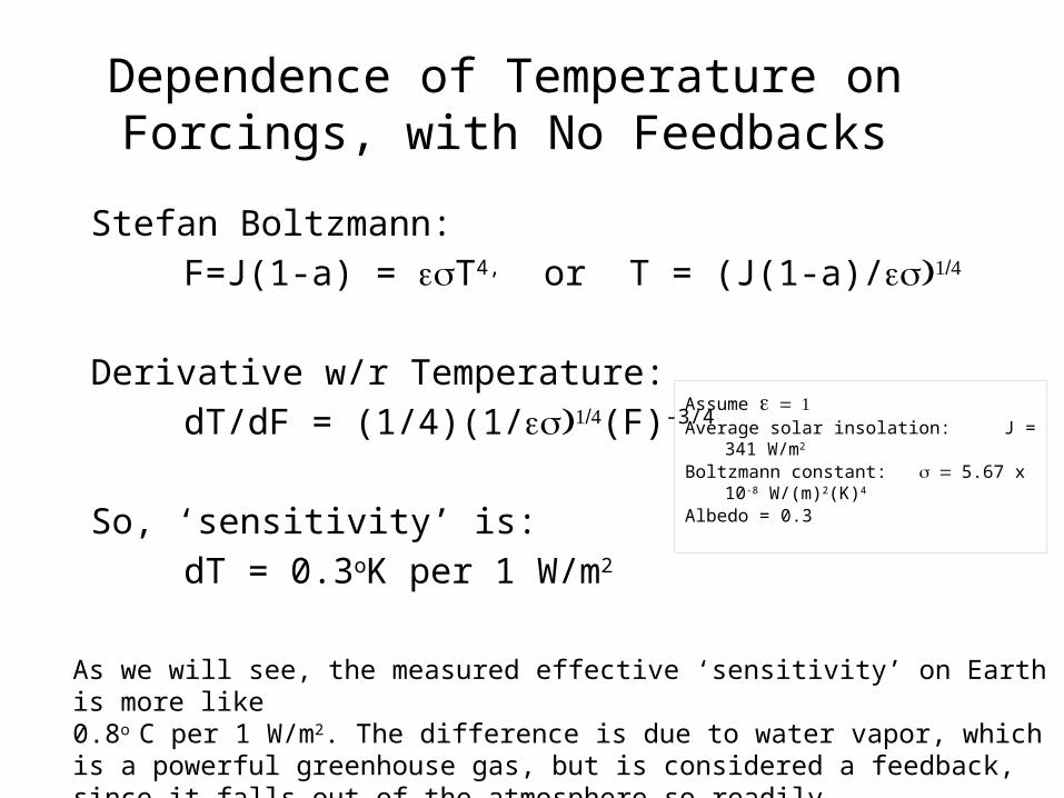
Dependence of Temperature on Forcings, with No Feedbacks
Stefan Boltzmann: F=J(1-a) = esT4, or T = (J(1-a)/ )es 1/4
Derivative w/r Temperature: dT/dF = (1/4)(1/ )es 1/4(F)-3/4
So, ‘sensitivity’ is:dT = 0.3oK per 1 W/m2
Assume e = 1 Average solar insolation: J = 341 W/m2
Boltzmann constant: = s 5.67 x 10⁻⁸ W/(m)2(K)4
Albedo = 0.3
As we will see, the measured effective ‘sensitivity’ on Earth is more like 0.8o C per 1 W/m2. The difference is due to water vapor, which is a powerful greenhouse gas, but is considered a feedback, since it falls out of the atmosphere so readily.
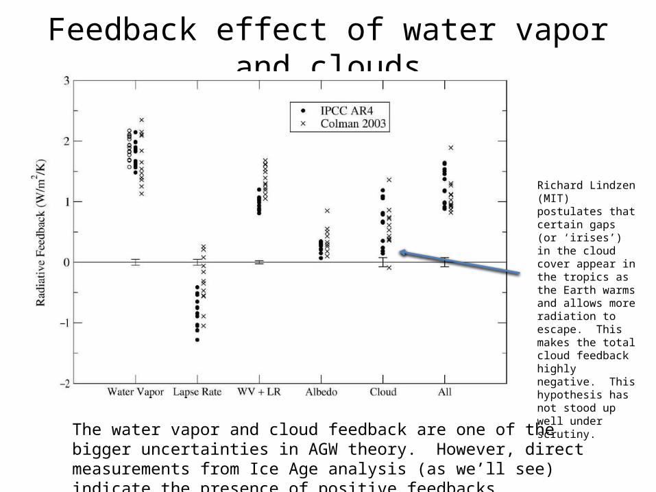
Feedback effect of water vapor and clouds
The water vapor and cloud feedback are one of the bigger uncertainties in AGW theory. However, direct measurements from Ice Age analysis (as we’ll see) indicate the presence of positive feedbacks.
Richard Lindzen (MIT) postulates that certain gaps (or ‘irises’) in the cloud cover appear in the tropics as the Earth warms and allows more radiation to escape. This makes the total cloud feedback highly negative. This hypothesis has not stood up well under scrutiny.
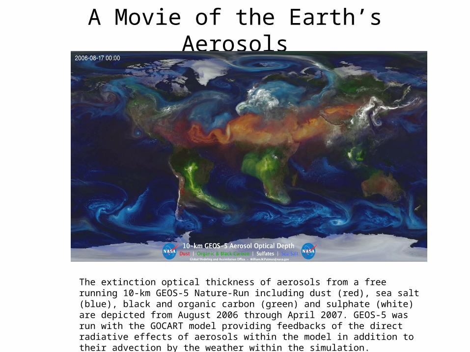
A Movie of the Earth’s Aerosols
The extinction optical thickness of aerosols from a free running 10-km GEOS-5 Nature-Run including dust (red), sea salt (blue), black and organic carbon (green) and sulphate (white) are depicted from August 2006 through April 2007. GEOS-5 was run with the GOCART model providing feedbacks of the direct radiative effects of aerosols within the model in addition to their advection by the weather within the simulation.

The Ice Ages
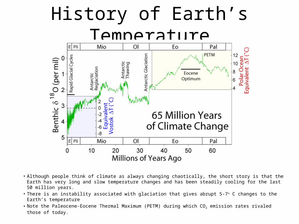
History of Earth’s Temperature
• Although people think of climate as always changing chaotically, the short story is that the Earth has very long and slow temperature changes and has been steadily cooling for the last 50 million years.
• There is an instability associated with glaciation that gives abrupt 5-7o C changes to the Earth’s temperature• Note the Paleocene-Eocene Thermal Maximum (PETM) during which CO2 emission rates rivaled those of today.
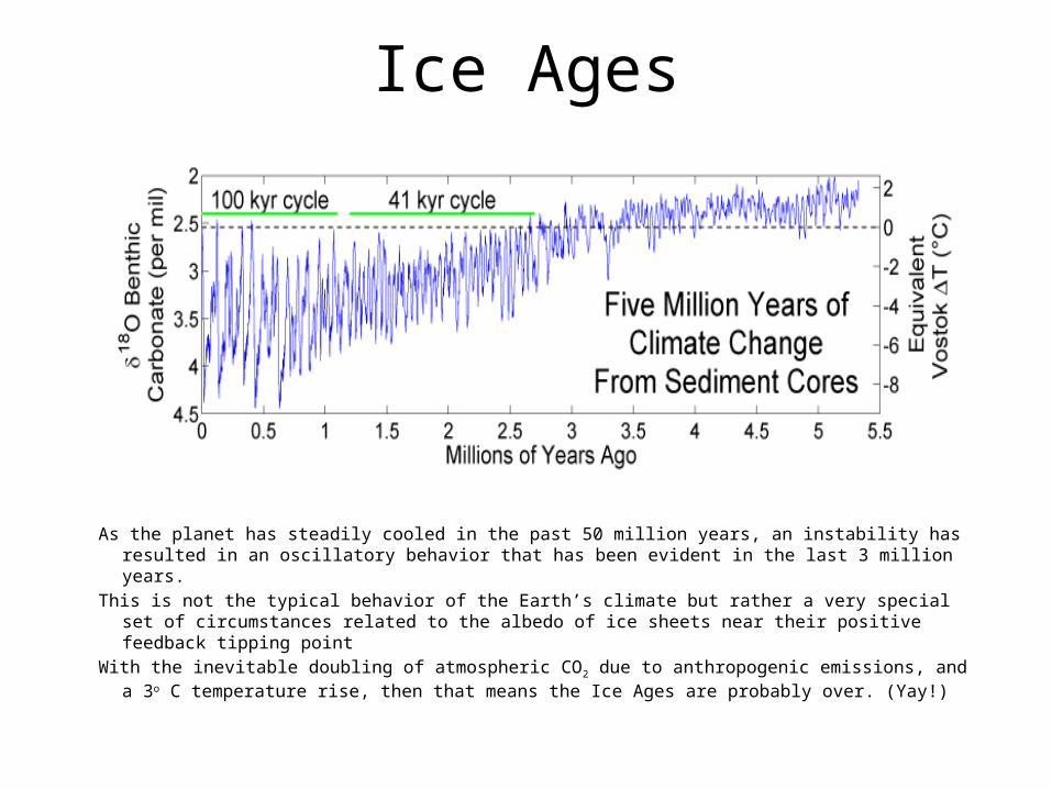
Ice Ages
As the planet has steadily cooled in the past 50 million years, an instability has resulted in an oscillatory behavior that has been evident in the last 3 million years.
This is not the typical behavior of the Earth’s climate but rather a very special set of circumstances related to the albedo of ice sheets near their positive feedback tipping point
With the inevitable doubling of atmospheric CO2 due to anthropogenic emissions, and a 3o C temperature rise, then that means the Ice Ages are probably over. (Yay!)
Milankovitch Cycles
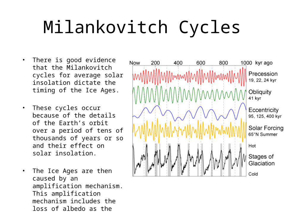
• There is good evidence that the Milankovitch cycles for average solar insolation dictate the timing of the Ice Ages.
• These cycles occur because of the details of the Earth’s orbit over a period of tens of thousands of years or so and their effect on solar insolation.
• The Ice Ages are then caused by an amplification mechanism. This amplification mechanism includes the loss of albedo as the ice sheets melt, and the release of greenhouse gases, specifically CO2, from the ocean.
400
420
440
460
480
500
520
540
0
0.2
0.4
0.6
0.8
1
1.2
1.4
0 100 200 300 400 500 600 700 800
Kyr Before Present
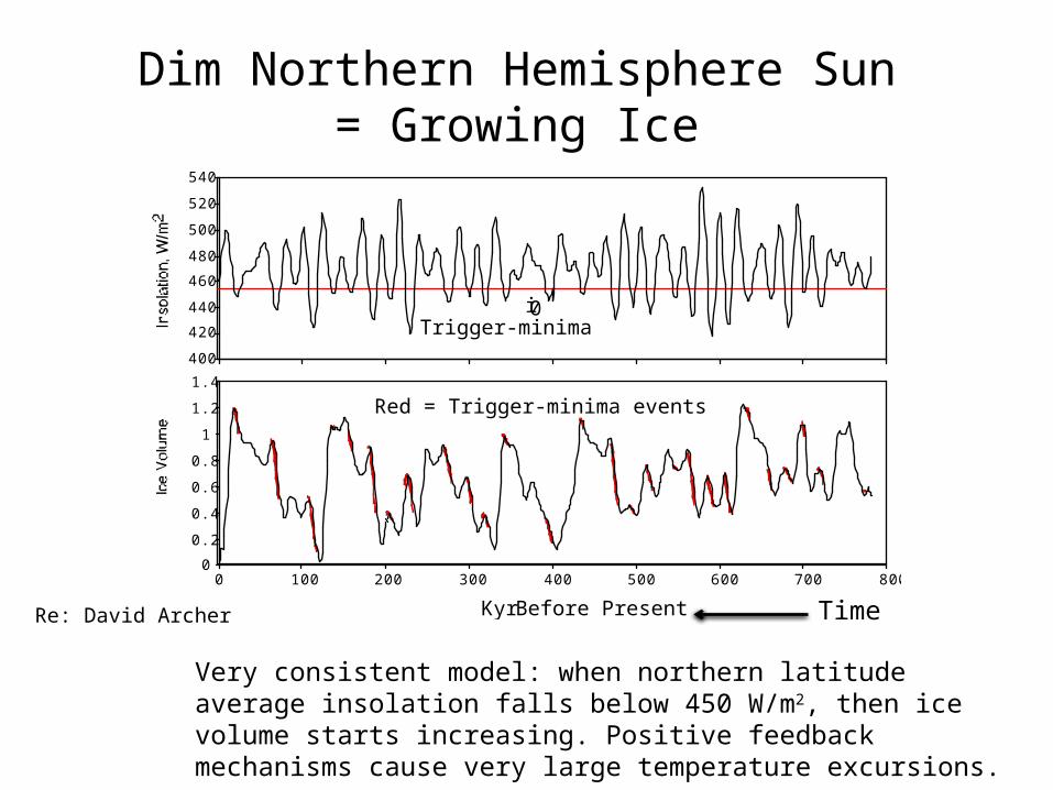
i0Trigger-minima
Red = Trigger-minima events
Dim Northern Hemisphere Sun= Growing Ice
Time
Very consistent model: when northern latitude average insolation falls below 450 W/m2, then ice volume starts increasing. Positive feedback mechanisms cause very large temperature excursions.
Re: David Archer
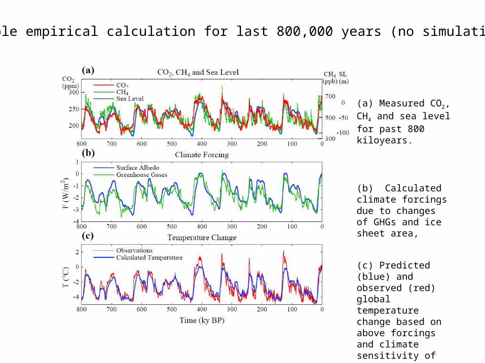
(a) Measured CO2, CH4 and sea level for past 800 kiloyears.
(b) Calculated climate forcings due to changes of GHGs and ice sheet area,
(c) Predicted (blue) and observed (red) global temperature change based on above forcings and climate sensitivity of ¾°C per W/m2. Observations are Antarctic T change divided by two.
Simple empirical calculation for last 800,000 years (no simulations)
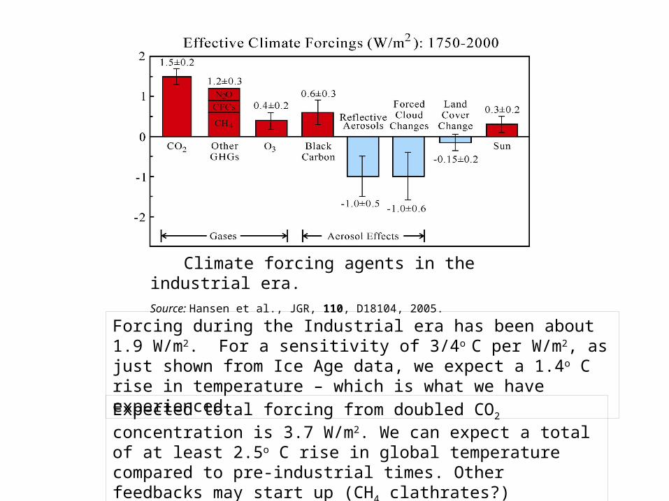
Climate forcing agents in the industrial era. Source: Hansen et al., JGR, 110, D18104, 2005.
Expected total forcing from doubled CO2 concentration is 3.7 W/m2. We can expect a total of at least 2.5o C rise in global temperature compared to pre-industrial times. Other feedbacks may start up (CH4 clathrates?)
Forcing during the Industrial era has been about 1.9 W/m2. For a sensitivity of 3/4o C per W/m2, as just shown from Ice Age data, we expect a 1.4o C rise in temperature – which is what we have experienced.
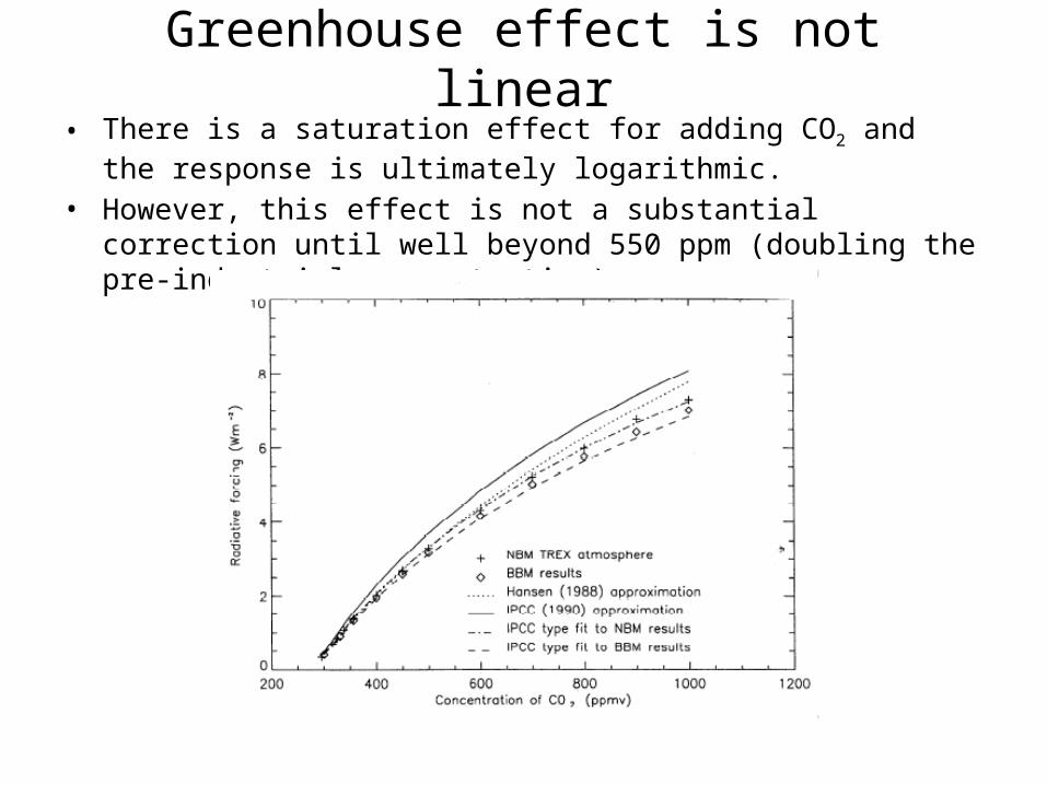
Greenhouse effect is not linear• There is a saturation effect for adding CO2 and the response is ultimately
logarithmic.• However, this effect is not a substantial correction until well beyond 550
ppm (doubling the pre-industrial concentration)
Measurements of Earth’s Temperature
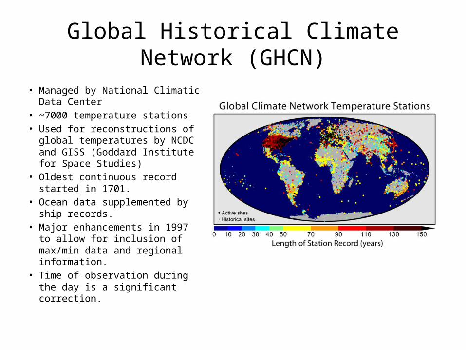
Global Historical Climate Network (GHCN)
• Managed by National Climatic Data Center
• ~7000 temperature stations• Used for reconstructions of global
temperatures by NCDC and GISS (Goddard Institute for Space Studies)
• Oldest continuous record started in 1701.
• Ocean data supplemented by ship records.
• Major enhancements in 1997 to allow for inclusion of max/min data and regional information.
• Time of observation during the day is a significant correction.
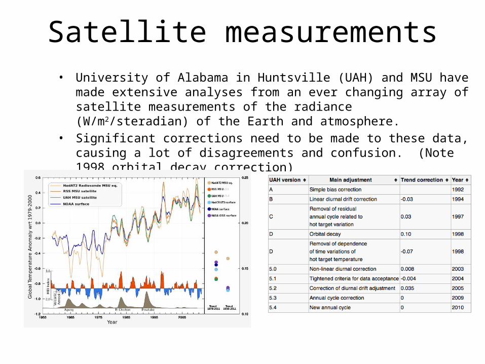
Satellite measurements• University of Alabama in Huntsville (UAH) and MSU have made extensive
analyses from an ever changing array of satellite measurements of the radiance (W/m2/steradian) of the Earth and atmosphere.
• Significant corrections need to be made to these data, causing a lot of disagreements and confusion. (Note 1998 orbital decay correction)
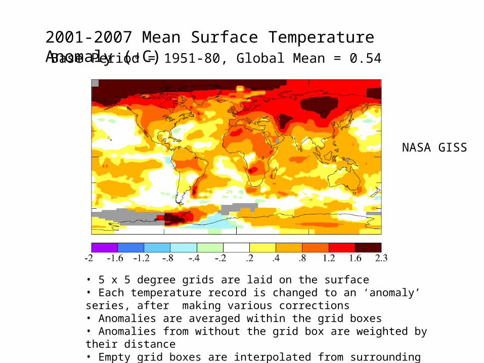
2001-2007 Mean Surface Temperature Anomaly (◦C)Base Period = 1951-80, Global Mean = 0.54
• 5 x 5 degree grids are laid on the surface• Each temperature record is changed to an ‘anomaly’ series, after making various corrections• Anomalies are averaged within the grid boxes• Anomalies from without the grid box are weighted by their distance• Empty grid boxes are interpolated from surrounding boxes
NASA GISS
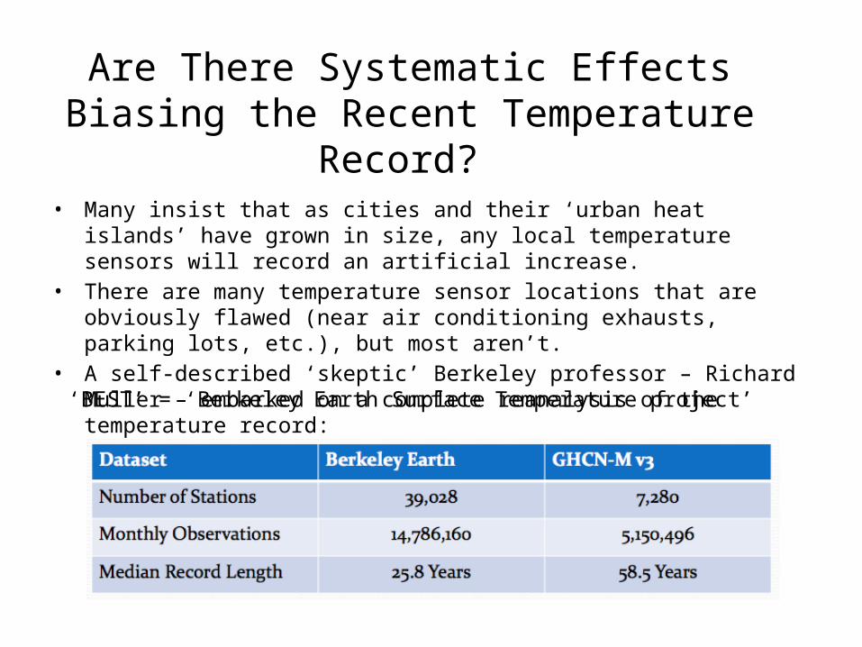
Are There Systematic Effects Biasing the Recent Temperature Record?
• Many insist that as cities and their ‘urban heat islands’ have grown in size, any local temperature sensors will record an artificial increase.
• There are many temperature sensor locations that are obviously flawed (near air conditioning exhausts, parking lots, etc.), but most aren’t.
• A self-described ‘skeptic’ Berkeley professor – Richard Muller – embarked on a complete reanalysis of the temperature record:
‘BEST’ = ‘Berkeley Earth Surface Temperature project’
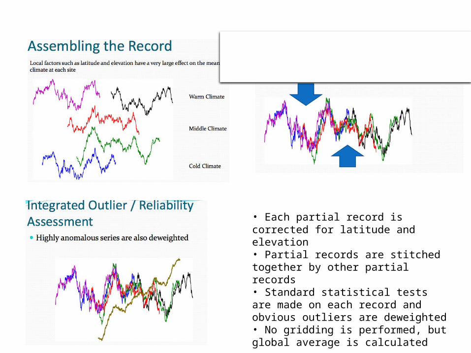
• Each partial record is corrected for latitude and elevation• Partial records are stitched together by other partial records• Standard statistical tests are made on each record and obvious outliers are deweighted• No gridding is performed, but global average is calculated
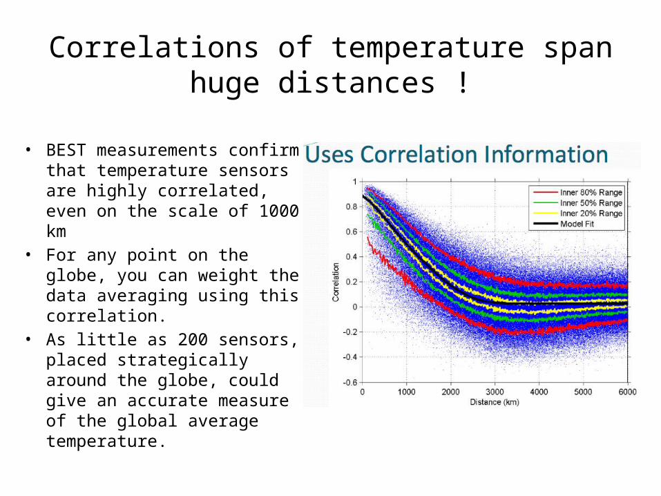
Correlations of temperature span huge distances !
• BEST measurements confirm that temperature sensors are highly correlated, even on the scale of 1000 km
• For any point on the globe, you can weight the data averaging using this correlation.
• As little as 200 sensors, placed strategically around the globe, could give an accurate measure of the global average temperature.
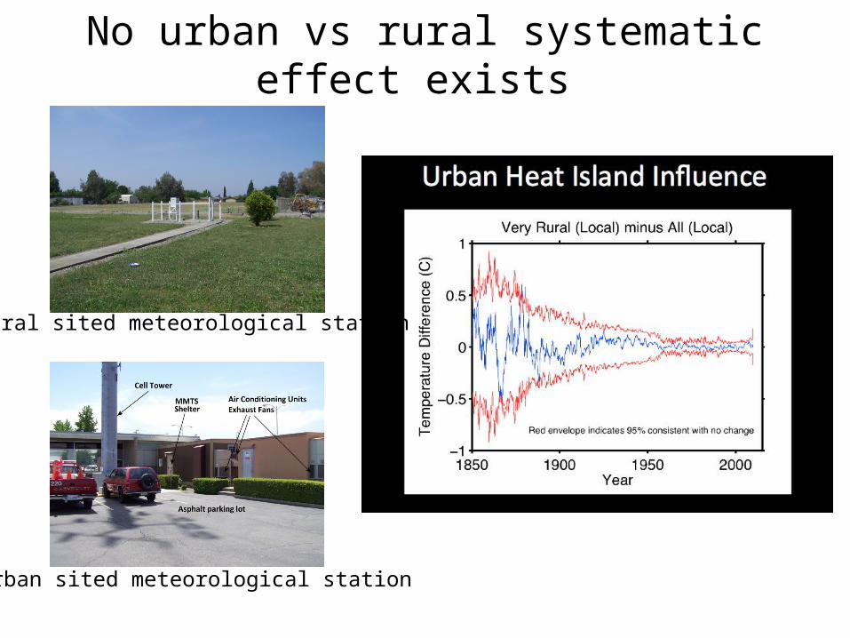
No urban vs rural systematic effect exists
Rural sited meteorological station
Urban sited meteorological station
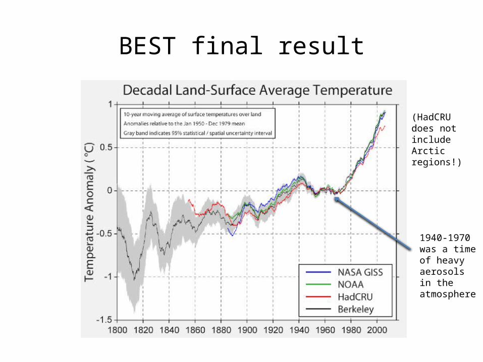
BEST final result
Strong warming signal showing no sign of slowing and fits profile of CO2 emission
(HadCRU does not include Arctic regions!)
1940-1970 was a time of heavy aerosols in the atmosphere
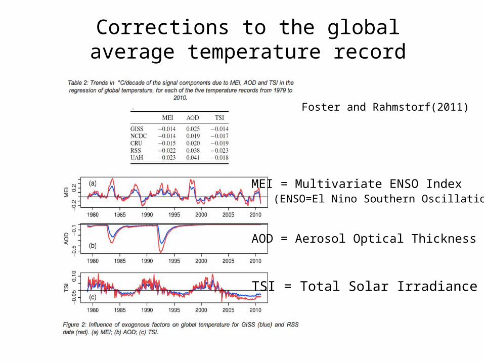
Corrections to the global average temperature record
MEI = Multivariate ENSO Index (ENSO=El Nino Southern Oscillation)
AOD = Aerosol Optical Thickness
TSI = Total Solar Irradiance
Foster and Rahmstorf(2011)
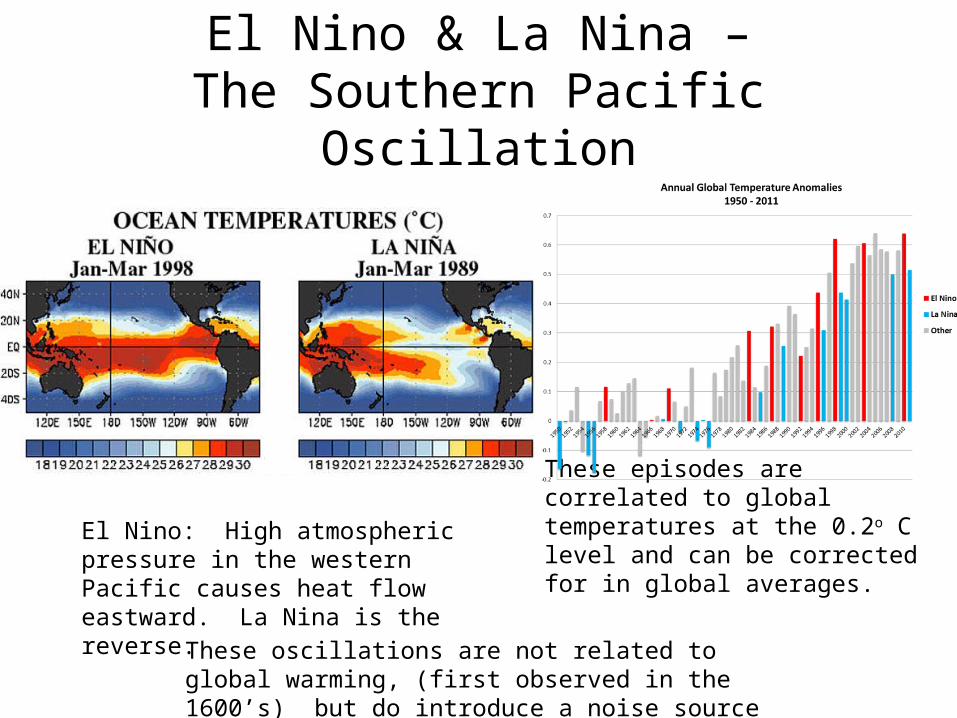
El Nino & La Nina –The Southern Pacific Oscillation
These episodes are correlated to global temperatures at the 0.2o C level and can be corrected for in global averages.
El Nino: High atmospheric pressure in the western Pacific causes heat flow eastward. La Nina is the reverse.
These oscillations are not related to global warming, (first observed in the 1600’s) but do introduce a noise source
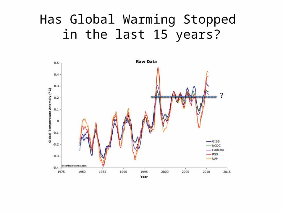
Has Global Warming Stopped in the last 15 years?
?
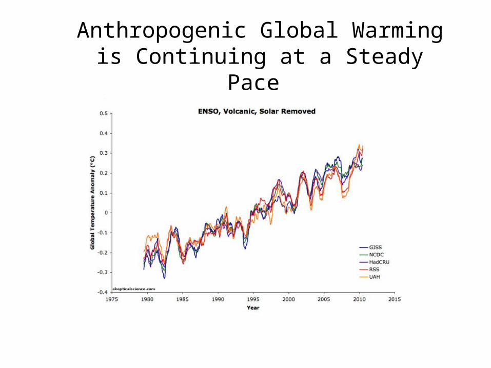
Anthropogenic Global Warming is Continuing at a Steady Pace
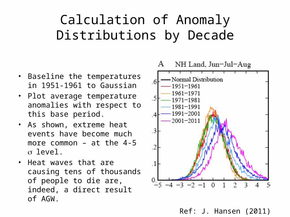
Calculation of Anomaly Distributions by Decade
• Baseline the temperatures in 1951-1961 to Gaussian
• Plot average temperature anomalies with respect to this base period.
• As shown, extreme heat events have become much more common – at the 4-5 s level.
• Heat waves that are causing tens of thousands of people to die are, indeed, a direct result of AGW.
Ref: J. Hansen (2011)

Water and Ice
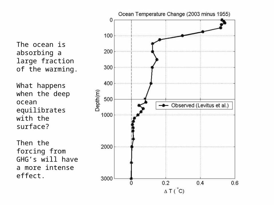
The ocean is absorbing a large fraction of the warming.
What happens when the deep ocean equilibrates with the surface?
Then the forcing from GHG’s will have a more intense effect.
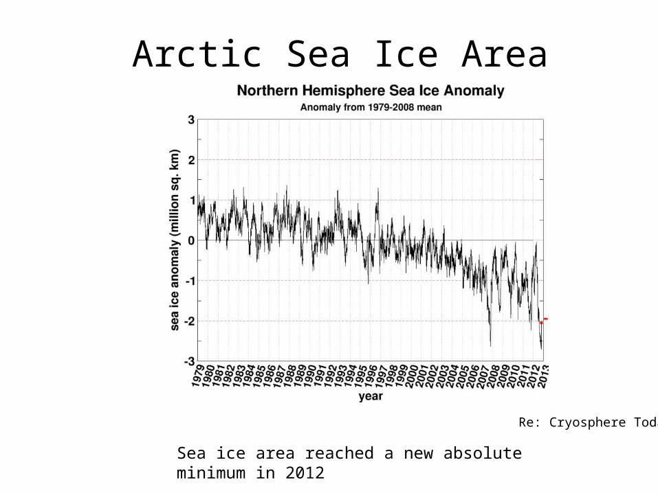
Arctic Sea Ice Area
Sea ice area reached a new absolute minimum in 2012
Re: Cryosphere Today
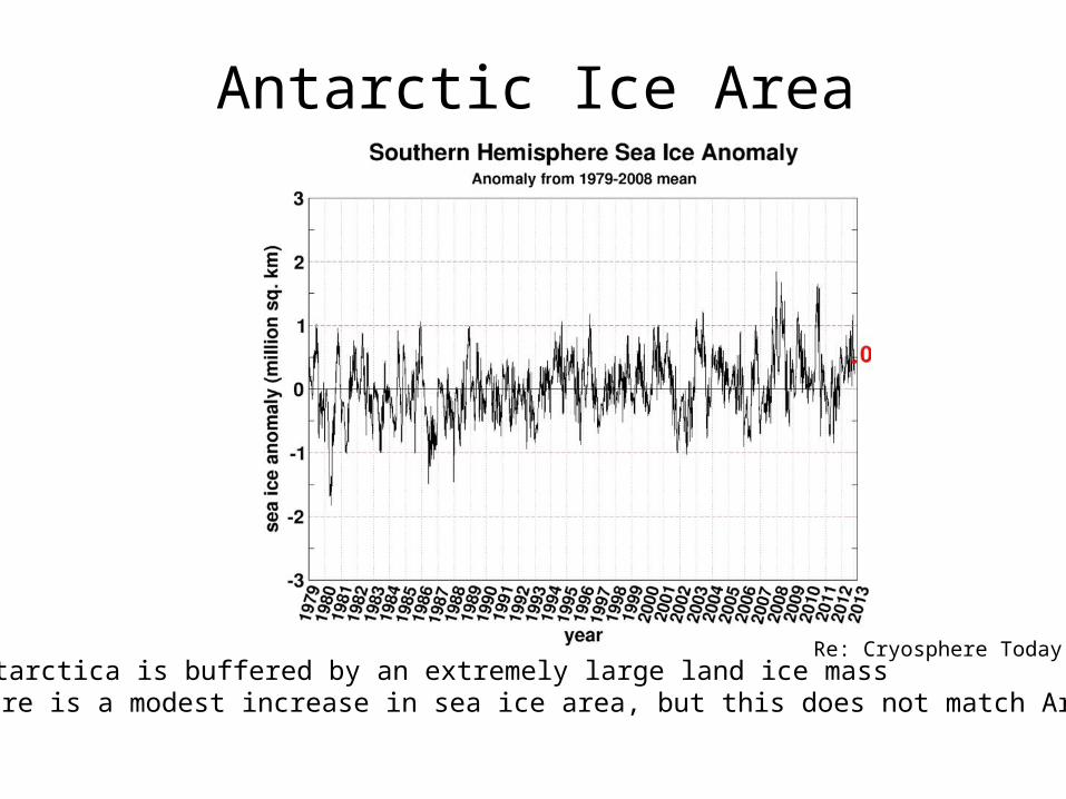
Antarctic Ice Area
- Antarctica is buffered by an extremely large land ice mass- There is a modest increase in sea ice area, but this does not match Arctic losses
Re: Cryosphere Today
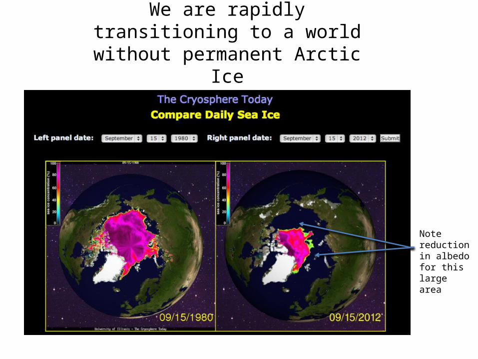
Note reduction in albedo for this large area
We are rapidly transitioning to a world without permanent Arctic Ice
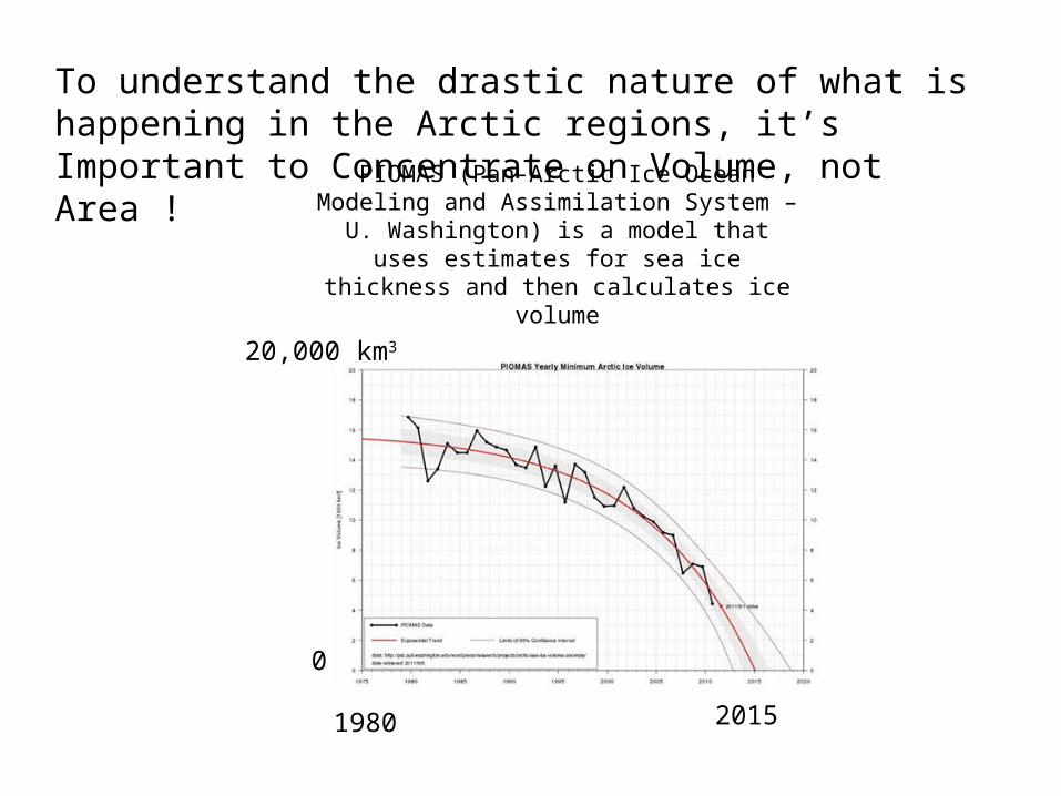
PIOMAS (Pan-Arctic Ice Ocean Modeling and Assimilation System – U. Washington) is a model that uses estimates for sea ice thickness and then
calculates ice volume
2015
To understand the drastic nature of what is happening in the Arctic regions, it’s Important to Concentrate on Volume, not Area !
0
20,000 km3
1980
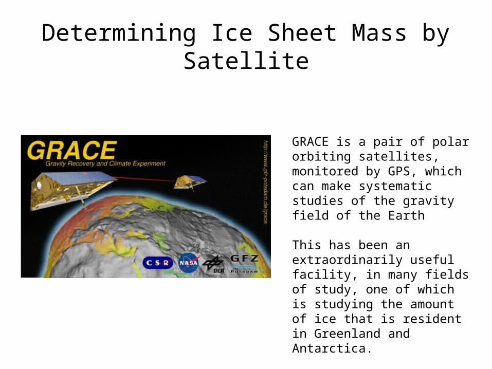
Determining Ice Sheet Mass by Satellite
GRACE is a pair of polar orbiting satellites, monitored by GPS, which can make systematic studies of the gravity field of the Earth
This has been an extraordinarily useful facility, in many fields of study, one of which is studying the amount of ice that is resident in Greenland and Antarctica.
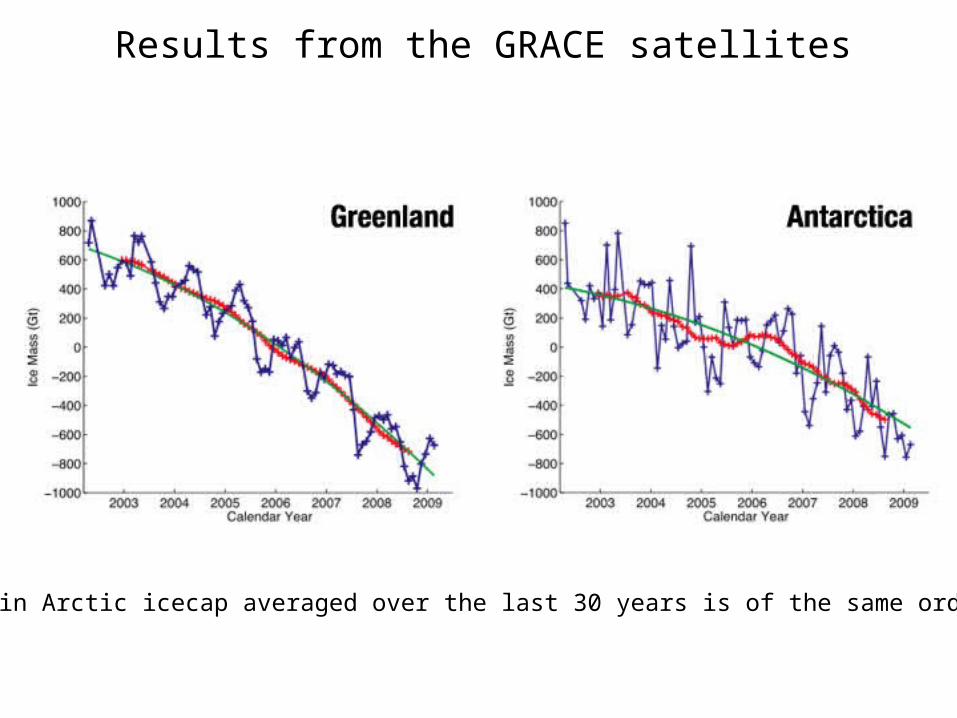
Results from the GRACE satellites
Loss in Arctic icecap averaged over the last 30 years is of the same order

The Future
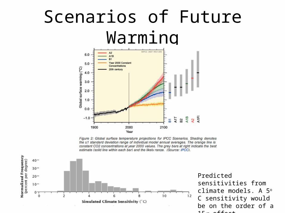
Scenarios of Future Warming
Predicted sensitivities from climate models. A 5o C sensitivity would be on the order of a 15s effect
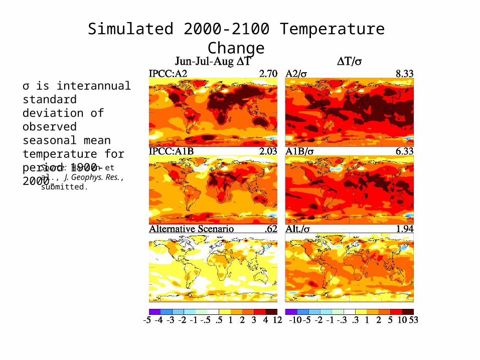
σ is interannual standard deviation of observed seasonal mean temperature for period 1900-2000.
Source: Hansen et al., J. Geophys. Res., submitted.
Simulated 2000-2100 Temperature Change
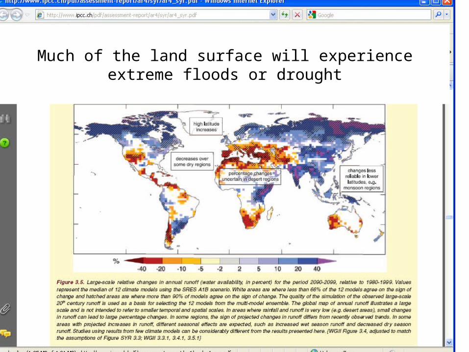
Much of the land surface will experience extreme floods or drought
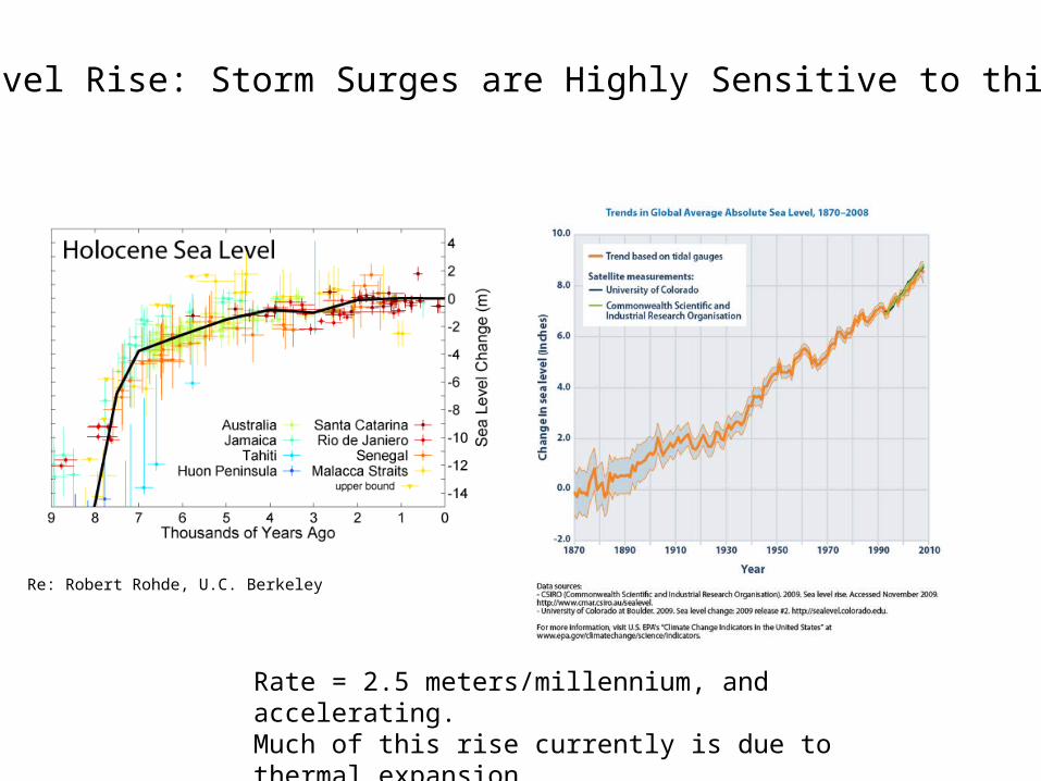
Sea Level Rise: Storm Surges are Highly Sensitive to this Value
Rate = 2.5 meters/millennium, and accelerating.Much of this rise currently is due to thermal expansion.
Re: Robert Rohde, U.C. Berkeley
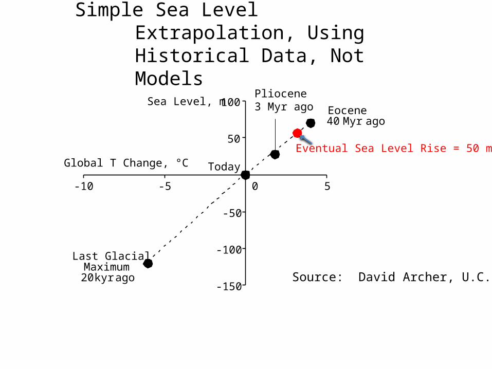
Simple Sea Level Extrapolation, Using Historical Data, Not Models
-150
-100
-50
50
100Sea Level, m
Last GlacialMaximum20 kyr ago
Eocene40 Myr ago
Today
Eventual Sea Level Rise = 50 m?!
Pliocene3 Myr ago
-10 -5 0 5
Global T Change, °C
Source: David Archer, U.C.
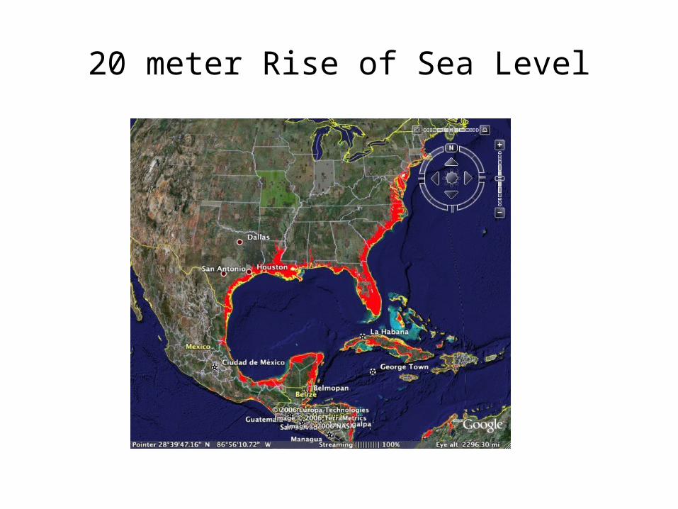
20 meter Rise of Sea Level
Facing the Problem
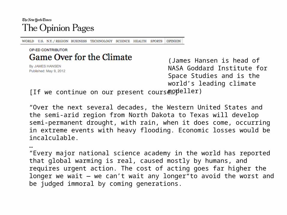
[If we continue on our present course…]
“Over the next several decades, the Western United States and the semi-arid region from North Dakota to Texas will develop semi-permanent drought, with rain, when it does come, occurring in extreme events with heavy flooding. Economic losses would be incalculable. …“Every major national science academy in the world has reported that global warming is real, caused mostly by humans, and requires urgent action. The cost of acting goes far higher the longer we wait — we can’t wait any longer to avoid the worst and be judged immoral by coming generations.”
(James Hansen is head of NASA Goddard Institute for Space Studies and is the world’s leading climate modeller)
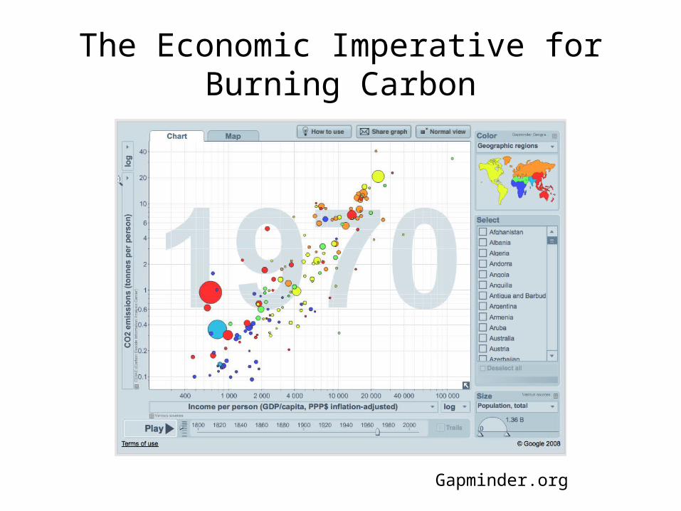
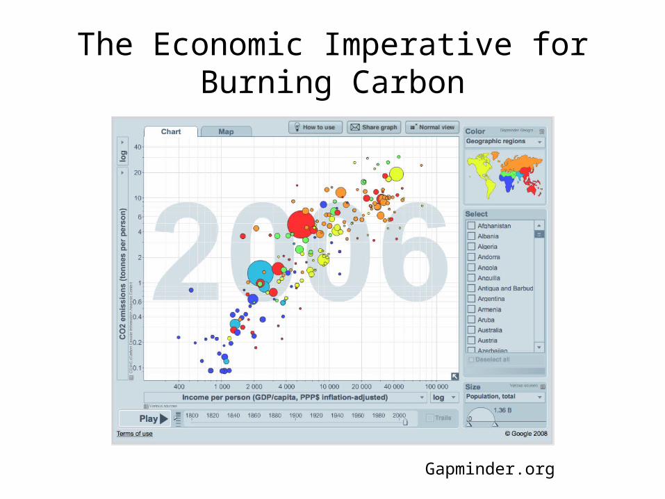
The Economic Imperative for Burning Carbon
Gapminder.org
The Economic Imperative for Burning Carbon
Gapminder.org
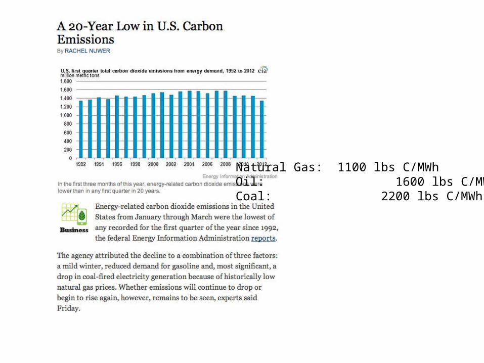
Natural Gas: 1100 lbs C/MWhOil: 1600 lbs C/MWhCoal: 2200 lbs C/MWh
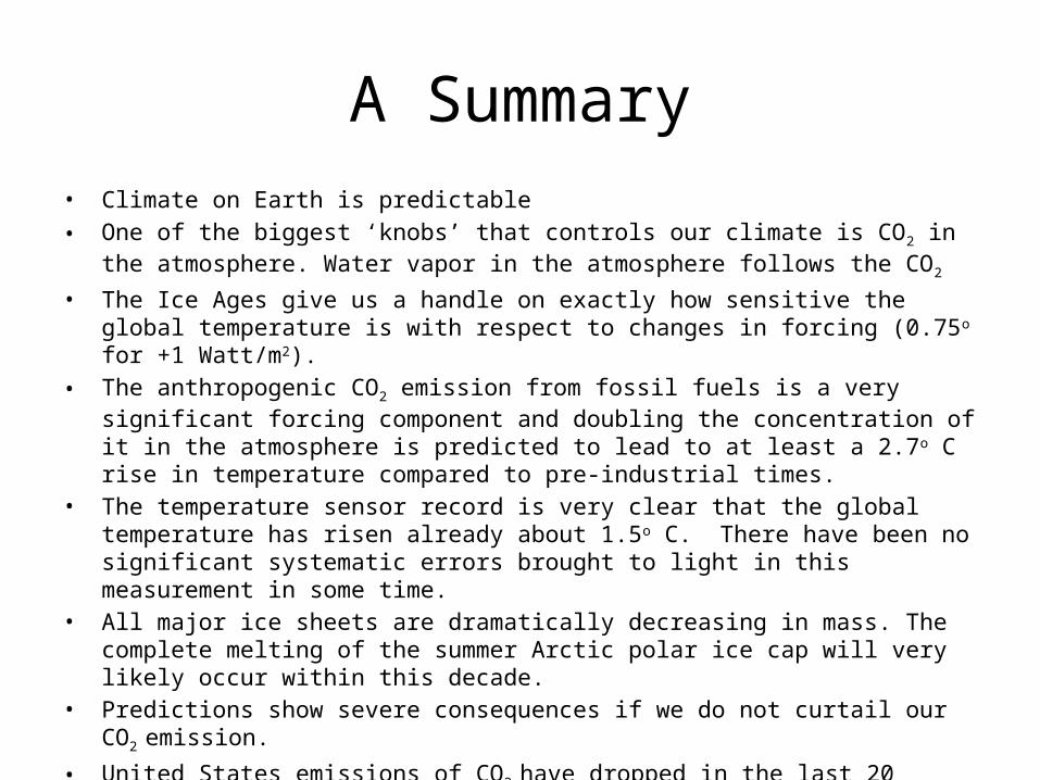
A Summary• Climate on Earth is predictable• One of the biggest ‘knobs’ that controls our climate is CO2 in the atmosphere. Water vapor in
the atmosphere follows the CO2
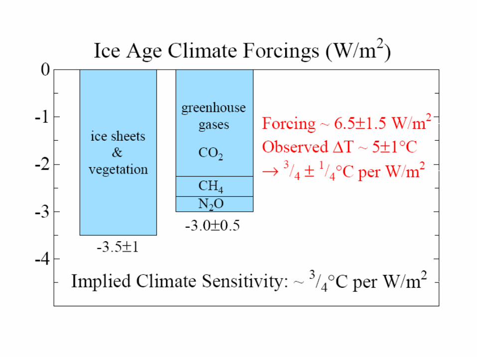
• The Ice Ages give us a handle on exactly how sensitive the global temperature is with respect to changes in forcing (0.75o for +1 Watt/m2).
• The anthropogenic CO2 emission from fossil fuels is a very significant forcing component and doubling the concentration of it in the atmosphere is predicted to lead to at least a 2.7o C rise in temperature compared to pre-industrial times.
• The temperature sensor record is very clear that the global temperature has risen already about 1.5o C. There have been no significant systematic errors brought to light in this measurement in some time.
• All major ice sheets are dramatically decreasing in mass. The complete melting of the summer Arctic polar ice cap will very likely occur within this decade.
• Predictions show severe consequences if we do not curtail our CO2 emission.
• United States emissions of CO2 have dropped in the last 20 years, so change is possible.• Every physicist should be familiar with the details of global climate change and be able to
confidently speak to the public about them.
Thank you for your attention!
If you are interested in talking about the solutions to anthropogenic global warming,
please join the:
Fermilab Sustainable Energy Club !Meeting tonight at 5:30 at User’s Center