co and non-co radiative forcings in climate projections

CO2 and non-CO2 radiative forcings in climate projectionsfor twenty-first century mitigation scenarios

Kuno M. Strassmann Æ G.-K. Plattner ÆF. Joos

Received: 14 April 2008 / Accepted: 28 November 2008 / Published online: 20 December 2008

� Springer-Verlag 2008

Abstract Climate is simulated for reference and mitiga-

tion emissions scenarios from Integrated Assessment Models

using the Bern2.5CC carbon cycle–climate model. Mitiga-

tion options encompass all major radiative forcing agents.

Temperature change is attributed to forcings using an

impulse–response substitute of Bern2.5CC. The contribution

of CO2 to global warming increases over the century in all

scenarios. Non-CO2 mitigation measures add to the abate-

ment of global warming. The share of mitigation carried by

CO2, however, increases when radiative forcing targets are

lowered, and increases after 2000 in all mitigation scenarios.

Thus, non-CO2 mitigation is limited and net CO2 emissions

must eventually subside. Mitigation rapidly reduces the

sulfate aerosol loading and associated cooling, partly

masking Greenhouse Gas mitigation over the coming dec-

ades. A profound effect of mitigation on CO2 concentration,

radiative forcing, temperatures and the rate of climate

change emerges in the second half of the century.

Keywords Climate projections � Mitigation scenarios �Attribution of climate change � Earth system models of

intermediate complexity � Carbon cycle

1 Introduction

This study assesses the role of individual radiative forcing

(RF) agents in climate change and mitigation of climate

change in emission scenarios for the twenty-first century.

Global mean surface temperature is a central proxy for

many of the impacts of climate change. We analyse the

contributions of individual RF agents to the magnitude and

the rate of temperature change over time, as well as the

mitigated temperature change. A particular emphasis is

placed on the rate of change in global mean temperature,

which codetermines the impact of climate change and the

costs of adaptation. By focusing on temperature rather than

RF we are able to capture time lags of the climate system

response. We also consider mitigation in the context of sea

level rise as an important impact on a longer timescale, and

of risks associated with high levels of CO2 through effects

other than global warming.

We investigate a set of reference and mitigation scenarios

for global emissions of the major anthropogenic greenhouse

gases (CO2, CH4, N2O, halocarbons, SF6), aerosol and

tropospheric ozone precursors (SO2, CO, NOx, VOCs)

throughout this century. Most of the scenarios were generated

as part of the Energy Modeling Forum project 21 (EMF-21)

(Weyant et al. 2006), with several Integrated Assessment

Models (IAM): AIM (Fujino et al. 2006), EPPA (Reilly et al.

2006), IMAGE (van Vuuren et al. 2006), IPAC (Jiang et al.

2006), MESSAGE (Rao and Riahi 2006), MiniCAM

(Smith and Wigley 2006). These IAMs are well known for

providing comprehensive scenarios to climate modellers,

inter alia the SRES illustrative scenarios used in the IPCC

reports (Nakicenovic and Swart 2000). Summary IAM model

descriptions are given in van Vuuren et al. (2008).

The EMF-21 project is a collaboration of modelling

groups assessing the potential of multigas mitigation

K. M. Strassmann (&) � F. Joos

Climate and Environmental Physics, University of Bern,

Sidlerstr. 5, 3012 Bern, Switzerland

e-mail: [email protected]

F. Joos

Oeschger Centre for Climate Change Research,

University of Bern, Bern, Switzerland

G.-K. Plattner

Institute of Biogeochemistry and Pollutant Dynamics,

ETH Zurich, Universitatstrasse 16, 8092 Zurich, Switzerland

123

Clim Dyn (2009) 33:737–749

DOI 10.1007/s00382-008-0505-4

CORE Metadata, citation and similar papers at core.ac.uk

Provided by RERO DOC Digital Library

https://core.ac.uk/display/159154799?utm_source=pdf&utm_medium=banner&utm_campaign=pdf-decoration-v1

policies. Before EMF-21, most attention in climate policy

modeling was paid to reducing CO2 emissions from the

energy sector. In EMF-21, special attention was given to

non-CO2 GHGs and CO2 sinks such as managed forests or

carbon capture and storage facilities (CCS). Some of the

IAMs participating in EMF-21 (MiniCAM, EPPA/ISGM,

MERGE) also provided the multigas scenarios described in

detail in Clarke et al. (2008).

The IAMs represented here feature representations of

the energy system and other parts of economy, such as

trade and agriculture, on varying levels of spatial and

process detail. Scenarios are generated by minimizing the

total systems costs under the constraints set by societal

drivers (population, welfare, technological innovation).

Most scenarios are related to SRES ‘‘storylines’’

(Nakicenovic and Swart 2000) (Table 1). Adding a con-

straint on radiative forcing leads to scenarios with policies

specifically aimed at mitigation (mitigation scenarios).

Mitigation policies can be assessed by comparing these

mitigation scenarios with corresponding scenarios that are

Table 1 Scenario overview. The SRES storyline is indicated where applicable; quantitative interpretations of storylines vary accross models

Target (Wm-2) EMFa RCPb Climate indicators for 2100

CO2 (ppm) CO2eqc (ppm) RF (Wm-2) RFmix

d (Wm-2) T (�C) dRFdt

Wm�2

10 years

� �dTdt

�C

10 years

� �

AIM (B2)

Ref 9 647 884 6.2 6.5 3.1 0.41 0.30

4.5 9 530 598 4.1 4.5 2.4 0.15 0.13

EPPA

Ref 900 1507 9.0 9.0 4.5 0.82 0.54

4.5 9 589 720 5.1 5.1 2.8 0.13 0.12

IMAGE (B2)

Ref 727 990 6.2 6.6 3.2 0.28 0.28

5.3 620 717 5.1 5.3 2.8 0.16 0.13

4.5 9 565 665 4.7 4.7 2.7 0.10 0.13

3.7 485 573 3.9 3.9 2.4 0.03 0.09

2.9 9 434 495 3.1 3.1 2.0 -0.10 0.01

2.6 9 400 457 2.7 2.6 1.8 -0.15 -0.02

IPAC (B2)

Ref 711 1008 6.9 7.0 3.4 0.39 0.26

4.5 9 552 725 5.1 5.1 2.8 0.11 0.11

MESSAGE (A2)

Ref 9 956 1773 9.9 9.9 4.9 0.89 0.50

4.5 510 694 4.9 4.9 2.8 -0.07 0.08

MESSAGE (B2)

Ref 665 1025 7.0 6.9 3.5 0.40 0.26

4.6 9 523 706 5.0 4.9 2.8 -0.18 0.05

3.2 401 522 3.4 3.3 2.3 -0.40 -0.07

MiniCam (B2)

Ref 759 956 6.6 6.6 3.3 0.49 0.39

4.5 561 642 4.5 4.5 2.7 0.08 0.12

4.5 9 9 586 670 4.7 4.7 2.8 0.08 0.13

4.0 516 585 4.0 4.0 2.4 0.02 0.09

3.5 478 537 3.5 3.6 2.2 -0.02 0.05

Radiative forcing targets corresponding to the year 2100 are indicated for mitigation scenarios. For each scenario, the values of key climate

indicators in the year 2100 are listed as simulated with standard model settings. Rates of change are means over the last decade of the century.

The calculation of CO2 and RF in IAMs and Bern2.5CC differs, therefore forcing targets do not necessarily equal the RF simulated herea Scenario for EMF-21 target of 4.5 Wm-2

b Selected as Representative Concentration Pathway scenario for the next IPCC report with possible minor modifications. The choice between

IMA2.6 and IMA2.9 is as yet undecidedc CO2 concentration equivalent for total RFd RF for well-mixed GHG, i.e. all forcings except aerosol and tropospheric O3

738 K. M. Strassmann et al.: CO2 and non-CO2 radiative forcings in climate projections

123

not constrained to a forcing target (reference scenarios).

The cost of climate change impacts is not explicitly con-

sidered in this scenario generation process.

The mitigation scenarios analysed here are constrained

by stabilization of total RF in the period 2100 to 2150 (RF

target). All IAMs provided a multigas mitigation scenario

with the common EMF-21 target of 4.5 Wm-2 with respect

to the preindustrial state (taken as the year 1765 in the

simulations). Additional scenarios are included with RF

targets ranging from 2.6 to 5.3 Wm-2 (Table 1).

IAMs draw on a wide range of technological options

representative of the current scientific debate to reduce GHG

emissions in mitigation scenarios. Feasibility of these tech-

nologies is an implied assumption and is not addressed

explicitly. This is true also for the reference scenarios, which

feature important efficiency improvements unprompted by

mitigation policies. It has been argued that baseline emis-

sions could be much higher if technological development is

less effective than assumed (Pielke et al. 2008). The feasi-

bility of additional improvements is presumably no less

uncertain. Riahi et al. (2007) have addressed these issues by

analyzing the contribution of selected technology clusters to

mitigation with respect to several reference scenarios and at

different levels of stringency. As already in Rao and Riahi

(2006), they emphasize the diversity of the mitigation port-

folio, but also demonstrate that carbon sink technologies are

consistently part of solutions to stringent forcing constraints.

All IAMs represented here include options for non-CO2

mitigation that are cheaper than CO2 mitigation, and the

multigas mitigation scenarios generally imply lower costs

than corresponding CO2-only scenarios (Fujino et al. 2006;

Jiang et al. 2006; Rao and Riahi 2006; Reilly et al. 2006;

Smith and Wigley 2006; van Vuuren et al. 2006). On the

other hand, non-CO2 mitigation potentials are bounded by

the total amount of non-CO2 emissions in the reference

scenarios, which remain inferior to the required CO2

reduction over the century. Since models minimize miti-

gation costs, they produce mitigation scenarios that begin

mostly with reductions of non-CO2 gases and then follow

with more expensive CO2 mitigation. This is a well-known

result that has been reported by several participant groups

in EMF-21 (e.g., Rao and Riahi 2006; Smith and Wigley

2006; van Vuuren et al. 2006). Here we explore how this

evolution of the mitigation portfolio affects global mean

surface temperatures in mitigation scenarios.

Mitigation scenarios have been widely used to investi-

gate options and measures to ‘‘achieve stabilization of

greenhouse gas concentrations in the atmosphere at a level

that would prevent dangerous interference with the climate

system’’ (United Nations 1992). Comprehensive multigas

mitigation scenarios as used in this paper, however, have

only recently become available. Earlier mitigation scenar-

ios are much less comprehensive in terms of relevant

processes and forcing agents considered. They focus

strongly on CO2, and only a few consider non-CO2 agents

(Schimel et al. 1997; Metz et al. 2001).

The working group I parts of the IPCC Third and Fourth

Assessment reports (TAR, AR4) discuss CO2 concentration

stabilization profiles, which implicitly are mitigation sce-

narios (Enting et al. 1994; Wigley et al. 1996; Prentice

et al. 2001; Cubasch et al. 2001; Meehl et al. 2007; Platt-

ner et al. 2008). In contrast to the emission scenarios used

here, in CO2 stabilization profiles the CO2 emissions are

inferred in a top-down manner from predefined concen-

trations. The role of non-CO2 GHGs in mitigation and

stabilization is not considered. Neither of the two IPCC

working group I reports include climate projections based

on bottom-up multigas mitigation scenarios, which infer

emissions from general development trends through

explicit and detailed modelling of technological processes.

Some participant groups in EMF-21 have reported results

from climate projections of their IAM in the EMF-21

special issue on multigas scenarios. A more detailed

investigation of climate projections for multigas scenarios

has been published recently for three IAMs (MiniCAM,

EPPA/ISGM, MERGE) by Levy II et al. (2008).

We further analyse climate projections for a set of ref-

erence and mitigation scenarios from six different IAMs

(Table 1). Included are scenarios earmarked for simula-

tions with Earth System Models (ESM) and Earth System

models of intermediate complexity (EMIC) for the next

IPCC Assessment report (AR5), termed Representative

Concentration Pathways (RCP, Table 1). By using one

EMIC to simulate RF and temperature across emission

scenarios from a group of different IAMs, it is possible to

separate general robust trends from model-dependent fea-

tures. The range of global temperature projections for these

mitigation and reference scenarios is discussed in van

Vuuren et al. (2008). Here we show how the different

forcings (GHG and aerosols) give rise to the projected

temperature evolution over this century, and how each of

them affects this path as a result of various degrees of

mitigation efforts. Specifically, we analyse (1) the contri-

bution of forcing agents to climate change in the past and

up to 2100, (2) the role of forcing agents for mitigation, (3)

the mitigation effect on the rate of global mean temperature

change and the contribution of individual RF agents to the

overall warming rate.

2 Methods

2.1 Model

We use the Bern2.5CC EMIC to calculate RF and climate

change from the emissions scenarios across the different

K. M. Strassmann et al.: CO2 and non-CO2 radiative forcings in climate projections 739

123

IAMs, using the same model setup as in van Vuuren et al.

(2008). Most IAMs contain simple climate–carbon cycle

model formulations, often based on MAGICC (Wigley and

Raper 2001) or the Bern substitute model (Joos et al.

1996). By using one model for the carbon cycle–climate

simulation we avoid differences that may arise from the

somewhat different climate–carbon cycle representations

within the IAMs.

Model components represent (1) the physical climate

system, (2) the cycling of carbon and related elements, and

(3), RF by atmospheric CO2, non-CO2 greenhouse gases

(GHG) and aerosols (Plattner et al. 2001; Joos et al. 2001).

The model setup used here includes only anthropogenic RF,

solar variability and volcanism are not considered. Solar

forcing over the twentieth century has been much smaller

than the anthropogenic GHG forcing and reliable prediction

of twenty-first century solar and volcanic forcing is lacking.

Apart from surface temperature, steric sea level rise,

mostly a result of thermal expansion, is also calculated in

Bern2.5CC. The Bern2.5CC steric sea level rise tends to be

high in comparison with, e.g., the CMIP (Meehl et al.

2005) group of Atmosphere–Ocean General Circulation

models (AOGCMs; Plattner et al. 2008), particularly when

the Atlantic meridional overturning circulation (AMOC),

which is sensitive in the model, shuts down (Knutti and

Stocker 2000). We note that contributions from changes in

ice sheets, alpine glaciers, and other terrestrial water stor-

age are not taken into account here.

CO2 RF is parametrized according to Myhre et al.

(1998), as described in Joos et al. (2001) and used in

Forster et al. (2007). RF of non-CO2 GHGs is calculated as

the product of concentrations and radiative efficiencies as

given in Forster et al. (2007). Non-CO2 concentrations are

modelled with first-order decay and atmospheric residence

times partly depending on concentrations of other gases

(Prather et al. 2001). The RF of aerosols, which have very

short residence times, is modelled as proportional to aero-

sol precursor emissions. For sulfate aerosols, SO2 emis-

sions are used, for organic and black carbon (OC/BC)

aerosols, CO emissions are used as a proxy of incomplete

combustion. The best estimates of aerosol forcing effi-

ciencies (Forster et al. 2007), used for the simulations

shown here, imply an important role of aerosols in the

anthropogenic influence on climate. Aerosol RF in the

scenarios used in this study is mostly due to sulfate aerosol.

The remainder is a positive RF from organic and black

carbon, which accounts for just a few percents. The RF by

individual aerosol types and processes is uncertain, but

total aerosol RF is constrained by observations and climate

model simulations (Forster et al. 2007). A detailed account

of the non-CO2 RF model is given in Joos et al. (2001).

Radiative efficiencies and life times are updated according

to Forster et al. (2007).

Feedbacks of atmospheric CO2 and climate on carbon

fluxes are captured by the explicit representation of the

carbon cycle in the Bern2.5CC model. The atmospheric CO2

concentration affects carbon uptake through CO2 dissolu-

tion in the ocean and CO2 fertilization on land. The climate–

carbon cycle feedback arises from the dependence of soil

carbon decay on temperature, the response of the global

vegetation distribution to climate change, the temperature-

dependent solubility of CO2 in the ocean and changes in

surface-to-deep transport and in the marine biological cycle

(Joos et al. 1999; Joos et al. 2001; Plattner et al. 2001),

where the first of these factors is dominant in the model on a

centennial timescale. Feedbacks for the non-CO2 GHGs are

not modeled. For example, methane is not represented in the

carbon cycle model. A limited coverage of feedbacks is

provided by the atmospheric chemistry parametrizations.

The model reference case is obtained with the standard

setup of the carbon cycle model and an equilibrium climate

sensitivity of 3.2 K for a nominal doubling of CO2. Climate

and carbon cycle uncertainty (vertical bars in Fig. 1) is

bounded by ‘‘endmember’’ combinations of assumptions:

The uncertainty in climate sensitivity is accounted for by

additional simulations with sensitivities of 1.5�C (low) and

4.5�C (high). The low-CO2 case is obtained by applying an

efficiently mixing ocean and assuming heterotrophic res-

piration to be independent of global warming; the high-

CO2 case is obtained by applying an inefficiently mixing

ocean and capping CO2 fertilization after the year 2000. A

compound parameter uncertainty range was obtained by

combining low-CO2 with low climate sensitivity, and high-

CO2 with high climate sensitivity. The same approach was

used in IPCC TAR and AR4 (Meehl et al. 2007; Joos et al.

2001; Prentice et al. 2001).

Simulations start from an equilibrated model state for

the year 1765 with zero RF. Until 2000, CO2, CH4, and

N2O concentrations are prescribed according to ice core

data and atmospheric observations as compiled by Joos and

Spahni (2008); RF of the other non-CO2 forcing agents in

the past is calculated as described in Joos et al. (2001),

except for updated parametrizations as mentioned above,

and a newer estimate of SO2 emissions (Stern 2005). From

year 2000 onwards, simulations are driven by the emissions

of CO2 and non-CO2 GHGs and aerosol precursors from

the IAM scenarios. The scenarios were harmonized to a

common emission level in the year 2000, as described in

van Vuuren et al. (2008).

2.2 Attribution method

The value of partitioning anthropogenic climate change by

forcing agents lies in the separate consideration of gases or

aerosols with differing dynamics and a different level of

scientific understanding.


123

The need to deal with several components on an equal

footing is commonly addressed by using the Global

Warming Potential (GWP) measure. All scenario models

featured here except AIM rely on GWPs to compare and

substitute forcing agents (Weyant et al. 2006). GWPs,

though of practical use, are a limited concept that afford

comparability of different forcing agents only with

respect to a given time horizon, here 100 years. GHG

emissions equivalent in terms of GWPs cause similar heat

input to the climate system over 100 years, but the tem-

perature response at any given time may differ. An

alternative measure proposed for comparison of unit

emissions of different GHGs is the Global Temperature

Potential (GTP Shine et al. 2005). GTPs take the climate

response into account and are comparable in terms of

temperature, but also strongly dependent on the time

frame considered.

Some forcing agents have a well-known radiative effi-

ciency, and some agreement exists about their future

emission trajectory. Such is the case for the gases listed

under the Montreal Protocol (all scenarios assume a phase

out as defined in the protocol). On the other extreme,

aerosols are characterized by strongly scenario-depen-

dent, i.e., uncertain emissions and a poorly constrained

radiative efficiency. In the IPCC AR4, aerosol RF is still

assigned the greatest uncertainty of all forcing compo-

nents (Forster et al. 2007). By partitioning global

temperature change into contributions from different

forcings the varying uncertainties associated with each of

them can be considered.

The attribution of global temperature change to RF

agents requires that the individual effects are additive.

Forster et al. (2007) suggest that this is a good assumption,

as studies with several different GCMs ‘‘have found no

evidence of any nonlinearity for changes in GHGs and

sulphate aerosol’’. A linear approximation of the

Bern2.5CC climate model is given by the impulse–

response substitute formulation (Joos and Bruno 1996):

dT ¼ 1

aochc

Z t

t0

Rðt0Þ � dTðt0Þ R2�dT2�

� �rðt � t0Þdt0; ð1Þ

where dT is the deviation of global mean surface air

temperature from the preindustrial state, R is radiative

forcing, R2 9 is the RF for twice the preindustrial CO2

concentration, dT2 9 is the equilibrium temperature change

corresponding to R2 9 , r is an impulse–response function, c

is the heat capacity of water per unit volume, h is the depth

of the mixed ocean surface layer, aoc is the fraction of the

earth surface covered by oceans, and t is time. The impulse–

response function is given as

rðtÞ ¼ a0j þX5

i¼1

aije�t=sij j ¼ 1 if t\4 years

2 if t� 4 years

�; ð2Þ

where aij,sij are two sets of coefficients and time scales,

respectively. They define two functions for the short and

the long term response, which are matched around year 4.

The temperature response of the Bern2.5CC model is

not strictly linear, as ocean circulation can change in

response to climate change and lead to a feedback affecting

2

4

6

8

10

12

Year

Rad

iativ

e F

orci

ng (

Wm

- 2)

Atm

osph

eric

CO

2 (p

pm)

Year

Tem

pera

ture

Dev

iatio

n (K

)

AIM

IMAGEIPACMESSAGE (A2)MESSAGE (B2)MiniCAM

EPPA

2000 20600

2

4

5

1

3

2020 2040 210020802000 20602020 2040 210020802000 20602020 2040 21002080

300

400

500

600

700

800

900

Year

0

0.2

0.4

0.6

0.8

Sea

leve

l [m

]

Year

2000 20602020 2040 21002080

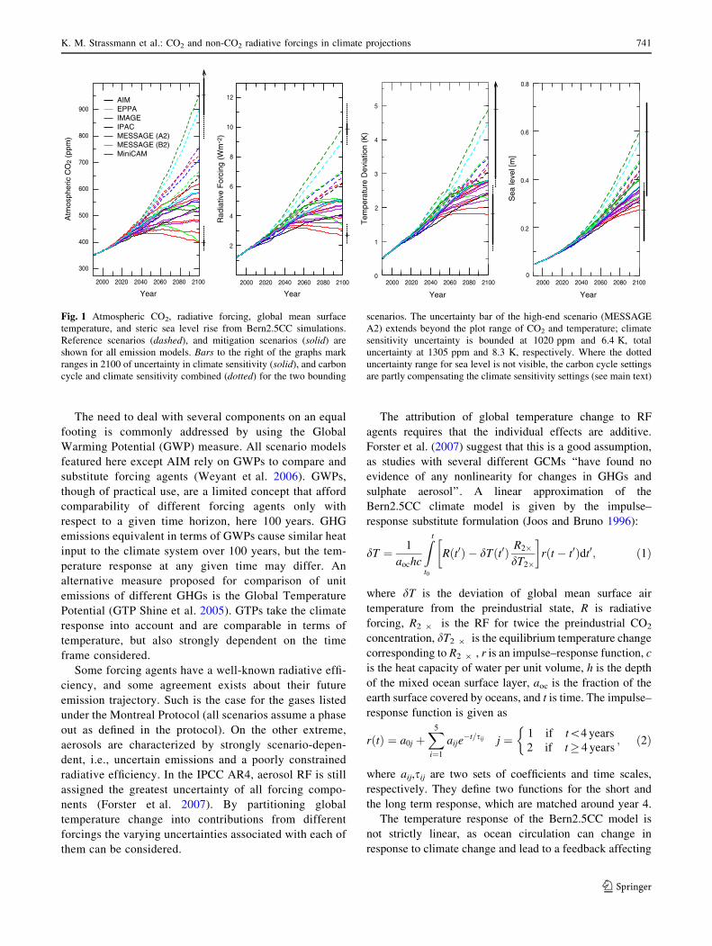
Fig. 1 Atmospheric CO2, radiative forcing, global mean surface

temperature, and steric sea level rise from Bern2.5CC simulations.

Reference scenarios (dashed), and mitigation scenarios (solid) are

shown for all emission models. Bars to the right of the graphs mark

ranges in 2100 of uncertainty in climate sensitivity (solid), and carbon

cycle and climate sensitivity combined (dotted) for the two bounding

scenarios. The uncertainty bar of the high-end scenario (MESSAGE

A2) extends beyond the plot range of CO2 and temperature; climate

sensitivity uncertainty is bounded at 1020 ppm and 6.4 K, total

uncertainty at 1305 ppm and 8.3 K, respectively. Where the dotted

uncertainty range for sea level is not visible, the carbon cycle settings

are partly compensating the climate sensitivity settings (see main text)


123

ocean heat uptake. Thus the substitute model does not

reproduce the temperature changes simulated with the origi-

nal Bern2.5CC perfectly. However, in the range of conditions

and timescales considered here, this nonlinearity is small

(Plattner et al. 2001), with substitute model temperatures at

2100 within 0.2�C of the complete model, except in the

sensitivity simulations with high climate sensitivity or low-

CO2 settings combined with high RF, where most substitute

simulations are about 0.5�C too small, and the ones with the

highest RF up to more than 1�C too small. This nonlinearity

arises due to strong changes in the AMOC which occur under

strong warming. However, for the scenarios considered

here, the relative contributions of different forcings are less

sensitive, because they are all similarly affected by the

deviation between Bern2.5CC and its substitute. Thus the

separation of the individual forcing contributions is reliable.

The global mean surface temperature change attribu-

table to each GHG or aerosol, dTi is obtained by solving

Eq. 1 for the corresponding forcing Ri, withP

idTi = dT

for the sum over all forcings.

In the standard setup of Bern2.5CC with a climate

sensitivity of dT2 9 = 3.2�C, global temperature change

affects ocean and land uptake of carbon, resulting in a

positive climate–carbon cycle feedback. This leads to

higher atmospheric CO2. The temperature change due to

CO2 without the carbon cycle–climate feedback is obtained

by inserting in Eq. 1 the RF corresponding to the atmo-

spheric CO2 from a Bern2.5CC simulation with climate

sensitivity set to zero in Bern2.5CC. The temperature

change in the standard simulation results from all anthro-

pogenic forcing agents including CO2, non-CO2 GHGs,

and aerosols.

The relationship between RF and climate change is

affected by the uncertainty in climate sensitivity. However,

this uncertainty affects all forcings in a similar way, except

for CO2, which is influenced by the climate–carbon cycle

feedback. The climate–carbon cycle feedback plays a

limited role in the results discussed here. The warmings

due to this feedback are governed by the main temperature

response of each scenario and vary accordingly. This vari-

ation among scenarios is small compared with the total

warming and does not greatly affect the temperature dif-

ferences between the scenarios in the standard model setup.

The feedback generally amplifies the general warming

trend and therefore does not introduce a qualitatively dif-

ferent behaviour (Fig. 2).

The carbon cycle uncertainty for the substitute simula-

tions was estimated using the RF from the Bern2.5CC

sensitivity simulations as described in Sect. 2.1.

A similar decomposition of temperature change for

different forcings has been done before, to allocate miti-

gation burdens according to historical responsibility for

climate change (den Elzen et al. 2005; den Elzen and

Schaeffer 2002; Trudinger and Enting 2005). This neces-

sitates an attribution of climate change to emissions, and,

unlike the RF-temperature relationship, involves essential

nonlinearities and a choice among several possible attri-

bution formalisms.

−1

01

23

45

∆T (

K)

ref

emf

AIM

ref

emf

IPAC

ref

emf

EPPA

refA

2

4.5

refB

2

emf

3.2

MESSAGE

ref

emf

4.5

4.0

3.5

MiniCAM

ref

emf

5.3

3.7

2.9

2.6

IMAGEyr 2

000

feedback

2O3 + Montreal Gases

6

3

CO2 without climate-C cycle feedbackClimate-C cycleCH4 + stratospheric HStratospheric ON2OOther halocarbons + SFTropospheric OSulfate + BC/OC Aerosols

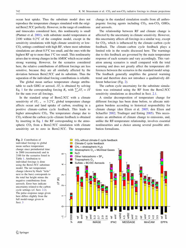
Fig. 2 Contribution of

individual forcings to global

mean surface temperature

change since preindustrial time

in 2000 (reconstructed) and in

2100 for the scenarios listed in

Table 1. Attribution to

individual forcings is done

using the Bern2.5CC substitute

model. The net temperature

change (shown by black ‘‘ticks’’

next to the bars) corresponds to

the total bar height minus the

negative contributions from

aerosols. Error bars indicate

uncertainty related to the carbon

cycle settings (cf. Sect. 2.2).

The pulse–response range given

here differs slightly from the

full model-range given in

Sect. 3


123

3 Results

The reference scenarios (Table 1) provide a range of

plausible future emissions in the absence of specific miti-

gation policies. These emissions lead to climate change

characterized by global mean surface air temperature rise

above preindustrial levels by the year 2100 of 3–3.5�C for

scenarios based on the B2 storyline and about 4.5–5�C for

others, not including the climate and carbon cycle model

uncertainty (Fig. 1; Table 1). The corresponding range in

RF is 6–7 Wm-2 (B2), and 9–10 Wm-2 (others), respec-

tively; the range in CO2 is 650–760 ppm (B2), and 900–

960 ppm (others), respectively.

The mitigation scenarios demonstrate that the imple-

mentation of technological measures and political

mechanisms for mitigation can have a profound impact on

the climate change expected under the same scenario sto-

rylines. The set of mitigation scenarios considered here

includes scenarios with radiative forcing targets from 2.6 to

5.3 Wm-2 (Fig. 1). Global temperature deviations in 2100

range from 1.8 to 2.8 K above preindustrial levels at the

standard climate sensitivity of 3.2�C. Simulated RF and

CO2 are in the range of 2.7–5.1 Wm-2 and 400–619 ppm,

respectively.

Trends in the year 2100 indicate that radiative forcing is

stabilized by the end of this century in many mitigation

scenarios (IMAGE 2.6–3.7 Wm-2, IPAC-EMF, MES-

SAGE-EMF), or close to stabilization (IMAGE 5.3 Wm-2,

EPPA-EMF, see Fig. 1). A number of mitigation scenarios

show a negative forcing trend in 2100 (IMAGE 2.6–2.9,

MESSAGE 3.2–4.6).

Temperatures respond to stabilizing RF levels with

some delay. While the temperatures for the more stringent

mitigation scenarios seem stable in 2100 or even declining,

the temperatures for the scenarios that comply with the

4.5 Wm-2 target of the EMF are still rising in 2100.

However, the rate of temperature increase and therefore of

climate change is greatly reduced with respect to the ref-

erence scenarios.

Sea level responds to global warming by thermal

expansion on centennial to millenial timescales. The con-

trast between the reference and mitigation scenarios

appears later than with temperature and evolves more

slowly, and accordingly, none of the mitigation scenarios

show a stabilized sea level in 2100. However, the simula-

tions still indicate a mitigation potential of 1–2 tenths of a

meter until 2100. The reference scenarios span a range of

0.41–0.60 m above the preindustrial sea level, as opposed

to 0.27–0.40 m for the mitigation scenarios. Further, steric

sea level rise is markedly decelerating in all mitigation

scenarios while in all the reference scenarios it is still

accelerating in 2100.

Thus, the magnitude and the rate of climate change and

steric sea level rise, as well as the trends at the turn of the

twent-second century show a substantial abatement due to

mitigation policies.

The uncertainty in carbon cycle and climate feedbacks

as defined in Sect. 2.1 strongly affects the effects and

impacts of emissions (Fig. 1). For example, for the MES-

SAGE A2-based reference scenario, the climate sensitivity

range of 1.5–4.5�C for a nominal doubling of CO2 in 2100

translates to a range of 883–1,015 ppm for atmospheric

CO2 and 2.9–6.4 �C for global mean surface temperature,

respectively. The carbon cycle uncertainty corresponds to a

range of 800–1213 ppm and 4.2–6.0�C, and the combined

climate–carbon cycle uncertainty to a range of 789–

1,305 ppm, and 2.6–8.3�C, respectively. For comparison,

the multimodel range of CO2 SRES-A2 projections from

the C4MIP project (Friedlingstein et al. 2006), is 730–

1,020 ppm in 2100. Non-CO2 RF is not included in

C4MIP, thus temperature projections are not comparable.

The likely (in the IPCC sense) range given in the IPCC

AR4 Summary for Policymakers for an A2 scenario is 2.7–

6.1�C above preindustrial for global mean surface air

temperature in the last decade of this century, assuming a

pre-2000 warming of 0.7�C, which corresponds to the

Bern2.5CC simulation with the standard setup and is

compatible with observations (Alley et al. 2007). Though

the feedback strength determining the absolute climate

response remains fairly uncertain, the contrast from refer-

ence to mitigation scenarios is qualitatively similar in any

setup.

The uncertainty range for steric sea level rise is related

to that of surface temperature, with two exceptions: (1) for

a time scale of one century it is more limited at the upper

end (0.72 m in 2100 for MESSAGE A2 reference) because

it takes more time to heat up the ocean, and (2) the carbon

cycle sensitivity settings have partly compensating effects:

In the low-CO2 case, for example, efficient ocean mixing

means relatively stronger ocean heat uptake and thermal

expansion, but at the same time, atmospheric CO2 and

surface temperatures driving sea level rise are lower, partly

due to increased ocean uptake, but mostly due to increased

land carbon storage. The converse applies to the high-CO2

case.

3.1 The contribution of forcing agents to climate

change in the past and in this century

In 2000, the most important GHG, CO2, accounts for about

the same global mean surface temperature change since

preindustrial as do the other GHGs combined. The simu-

lated cooling by aerosols in 2000 offsets about half of the

warming by all GHGs (Fig. 2).


123

However, the share of warming caused by CO2 increases

after the year 2000 in all scenarios. By 2100, it accounts for

twice the warming attributed to the non-CO2 GHGs or

more in many scenarios, particularly some mitigation

scenarios (cf. Sect. 3.2). Toward the end of the century, the

share of GHG warming attributable to CO2 decreases again

slightly only for the scenarios MESSAGE 3.2 (after 1960)

and MESSAGE 4.5 (after 1990). MESSAGE mitigation

scenarios feature the steepest reduction of net CO2 emis-

sions in the set. The climate–carbon cycle feedback

contributes to the growing influence of CO2. It is compa-

rable in magnitude to the individual non-CO2 GHGs.

The partitioning of non-CO2 GHG warming varies

across models. In the reference scenarios, generally CH4

ranks first, followed by tropospheric ozone, N2O, HFCs/

PFCs/SF6 and the Montreal gases and stratospheric ozone.

This pattern is less clear in the mitigation scenarios, as

different GHGs can be reduced at different rates. Never-

theless, in all cases CH4 is still the most important non-CO2

gas (cf. Sect. 3.2). Model-specific differences are apparent,

e.g., CH4 contributes a particularly large fraction of non-

CO2 warming in all MESSAGE scenarios.

Aerosol cooling peaked in the seventies, offsetting 75%

of GHG warming around 1970 (not shown). Since then,

global SO2 emissions have stagnated and eventually

declined according to the estimate used here (Stern 2005).

This decline is immediately expressed in aerosol RF,

leading to stagnating aerosol cooling while GHG warming

continued. The decline of SO2 emissions is projected to

continue into the future in reference and mitigation sce-

narios alike, while the OC/BC aerosol loading as estimated

here does not show consistent decrease. However, the net

positive forcing due to OC/BC aerosols never fully com-

pensates the sulfate aerosol cooling as simulated for any of

the scenarios.

3.2 The role of forcing agents in mitigation

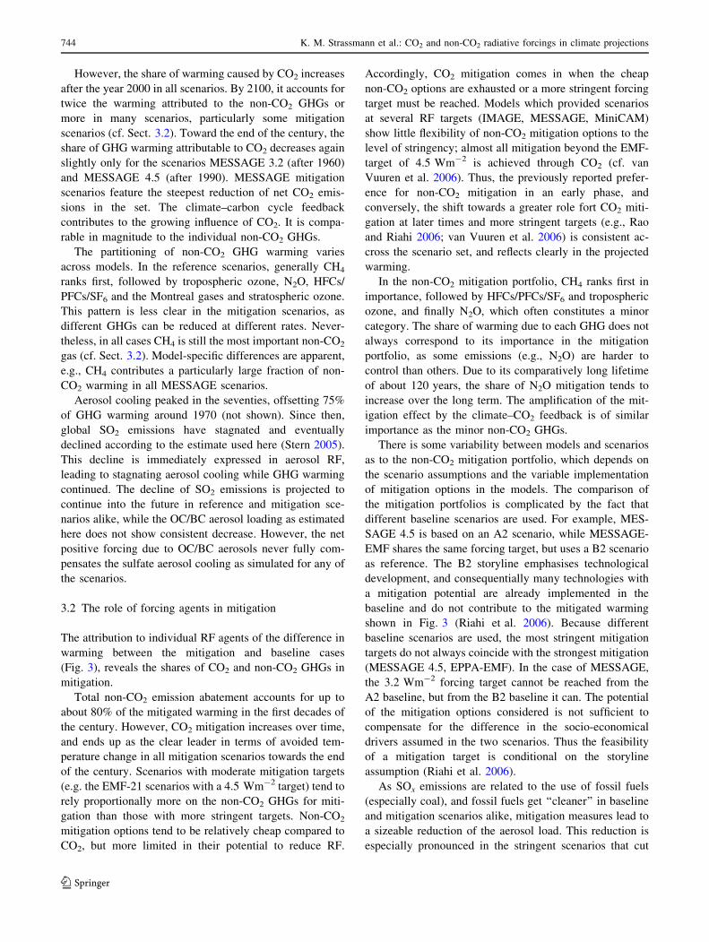
The attribution to individual RF agents of the difference in

warming between the mitigation and baseline cases

(Fig. 3), reveals the shares of CO2 and non-CO2 GHGs in

mitigation.

Total non-CO2 emission abatement accounts for up to

about 80% of the mitigated warming in the first decades of

the century. However, CO2 mitigation increases over time,

and ends up as the clear leader in terms of avoided tem-

perature change in all mitigation scenarios towards the end

of the century. Scenarios with moderate mitigation targets

(e.g. the EMF-21 scenarios with a 4.5 Wm-2 target) tend to

rely proportionally more on the non-CO2 GHGs for miti-

gation than those with more stringent targets. Non-CO2

mitigation options tend to be relatively cheap compared to

CO2, but more limited in their potential to reduce RF.

Accordingly, CO2 mitigation comes in when the cheap

non-CO2 options are exhausted or a more stringent forcing

target must be reached. Models which provided scenarios

at several RF targets (IMAGE, MESSAGE, MiniCAM)

show little flexibility of non-CO2 mitigation options to the

level of stringency; almost all mitigation beyond the EMF-

target of 4.5 Wm-2 is achieved through CO2 (cf. van

Vuuren et al. 2006). Thus, the previously reported prefer-

ence for non-CO2 mitigation in an early phase, and

conversely, the shift towards a greater role fort CO2 miti-

gation at later times and more stringent targets (e.g., Rao

and Riahi 2006; van Vuuren et al. 2006) is consistent ac-

cross the scenario set, and reflects clearly in the projected

warming.

In the non-CO2 mitigation portfolio, CH4 ranks first in

importance, followed by HFCs/PFCs/SF6 and tropospheric

ozone, and finally N2O, which often constitutes a minor

category. The share of warming due to each GHG does not

always correspond to its importance in the mitigation

portfolio, as some emissions (e.g., N2O) are harder to

control than others. Due to its comparatively long lifetime

of about 120 years, the share of N2O mitigation tends to

increase over the long term. The amplification of the mit-

igation effect by the climate–CO2 feedback is of similar

importance as the minor non-CO2 GHGs.

There is some variability between models and scenarios

as to the non-CO2 mitigation portfolio, which depends on

the scenario assumptions and the variable implementation

of mitigation options in the models. The comparison of

the mitigation portfolios is complicated by the fact that

different baseline scenarios are used. For example, MES-

SAGE 4.5 is based on an A2 scenario, while MESSAGE-

EMF shares the same forcing target, but uses a B2 scenario

as reference. The B2 storyline emphasises technological

development, and consequentially many technologies with

a mitigation potential are already implemented in the

baseline and do not contribute to the mitigated warming

shown in Fig. 3 (Riahi et al. 2006). Because different

baseline scenarios are used, the most stringent mitigation

targets do not always coincide with the strongest mitigation

(MESSAGE 4.5, EPPA-EMF). In the case of MESSAGE,

the 3.2 Wm-2 forcing target cannot be reached from the

A2 baseline, but from the B2 baseline it can. The potential

of the mitigation options considered is not sufficient to

compensate for the difference in the socio-economical

drivers assumed in the two scenarios. Thus the feasibility

of a mitigation target is conditional on the storyline

assumption (Riahi et al. 2006).

As SOx emissions are related to the use of fossil fuels

(especially coal), and fossil fuels get ‘‘cleaner’’ in baseline

and mitigation scenarios alike, mitigation measures lead to

a sizeable reduction of the aerosol load. This reduction is

especially pronounced in the stringent scenarios that cut


123

CO2 emissions early on (Fig. 3). In the first decades of the

twenty-first century, the warming due to SO2 emission

abatement rivals the cooling due to GHG mitigation in

many scenarios, especially those with stringent targets.

While aerosol abatement is a co-benefit for air pollution

reduction, it potentially lessens the impact of mitigation

measures in the early twenty-frist century (e.g., Smith and

Wigley 2006; van Vuuren et al. 2006). Furthermore, it

increases the uncertainty of climate projections over this

period. However, the warming due to aerosol abatement

tends to quickly stabilise, while GHG abatement leads to

increasing mitigation. This is due to the fact that in the

mitigation scenarios, the bulk of aerosol precursor emission

reductions occurs in the first half of the century and then

reaches a minimum level, while the reference scenarios

reduce less and later.

3.3 Warming rate and the role of forcing agents

The rate of change in temperature and other climatic

variables is an issue of importance quite independent of

that of the mitigation target and stabilization level. Rates of

change codetermine the impact of climate change and costs

of adaptation (e.g., Adger et al. 2007).

Mitigation does not show strong effects on temperature

evolution over several decades. Several factors explain this

slow start. The first is inertia in the climate system and

in the socio-technological system. The second is that the

−2.

5−

2.0

−1.

5−

1.0

−0.

50.

00.

5−

0.5

−0.

3−

0.1

0.0

0.1

∆T

20402070

2100

emf emf 5.3 3.7 2.9 2.6 emf 4.5 emf 3.2 emf 4.5 4.0 3.5 emf

AIM IMAGE IPAC MESSAGE MiniCAM EPPA

CO2 without climate-C cycle feedbackClimate-C cycle feedbackCH4 + stratospheric H2OStratospheric O3 + Montreal GasesN2OOther halocarbons + SF6

Tropospheric O3

Sulfate + BC/OC Aerosols

∆T/1

0 yr

Fig. 3 Effect of mitigation on

temperature change attributed to

individual forcings using the

Bern2.5CC substitute model.

The difference DT in global

mean surface temperature

between each mitigation

scenario and the corresponding

reference scenario is shown in

the top panel (DT = 0 in the

year 2000), and the difference in

the mean rate of change in the

bottom panel. Each three

adjacent bars correspond to

temperatures in 2040, 2070, and

2100, and to 25 year-average

rates from these dates

backwards, respectively. The

net temperature contrast due to

mitigation is shown by black

‘‘ticks’’


123

‘‘deadline’’ of the RF target is still too far to induce sub-

stantial mitigation efforts in the scenarios with moderate

targets. The third is sulfate aerosol abatement as discussed

in Sect. 3.2. Scenarios with stringent RF targets show

particularly rapid and strong SO2 emission abatement. Due

to the very short atmospheric lifetime of aerosols, high-

aerosol warming rates can result (Fig. 3, bottom). Conse-

quently, even in aggressive mitigation scenarios global

temperature increases at rates not far below the baseline

rates of change until the mid twenty-frist century (Fig. 4).

A similar result has been reported for the IMAGE (van

Vuuren et al. 2006) and for the MiniCAM scenarios (Smith

and Wigley 2006) using the climate component of these

IAMs (MAGICC).

The second half of the century only reveals the huge

difference between baseline and mitigation scenarios.

Some mitigation scenarios show a trend reversal in rates of

temperature change for certain forcings (particularly, CH4,

tropospheric and stratospheric O3 from IMAGE and

MiniCAM). Rates of temperature change due to CO2 are

strongly decreased in the more ambitious mitigation sce-

narios, and negative rates (including the climate–carbon

cycle feedback) are seen in the IMAGE 2.6 and the

MESSAGE 3.2 scenarios. This is the delayed response to

atmospheric CO2 levels receding since the 2050ies in these

scenarios as a result of major CO2 emission reductions.

While warming decelerates in mitigation scenarios as

stabilization at the forcing target is approached (-0.01 to

0.18�C /decade over the last 25 years), it further acceler-

ates in the references (0.26–0.54�C/decade). Thus the

substantial difference in the temperature levels reached in

2100 builds up during quite a short period. Looking further

2000 − 2025

∆T10

yr

−0.

10.

00.

10.

20.

30.

40.

5

2025 − 2050

∆T10

yr

−0.

10.

00.

10.

20.

30.

40.

5

2050 − 2075

∆T10

yr

−0.

10.

00.

10.

20.

30.

40.

5

2075 − 2100

∆T10

yr

−0.

10.

00.

10.

20.

30.

40.

5

ref

emf

ref

emf

5.3

3.7

2.9

2.6

ref

emf

refA

24.

5re

fB2

emf

3.2

ref

emf

4.5

4.0

3.5

ref

emf


ref

emf

ref

emf

5.3

3.7

2.9

2.6

ref

emf

refA

24.

5re

fB2

emf

3.2

ref

emf

4.5

4.0

3.5

ref

emf


CO2 without climate-C cycle feedbackClimate-C cycle feedbackCH4 + stratospheric H2OStratospheric O3 + Montreal GasesN2OOther halocarbons + SF6

Tropospheric O3

Sulfate + BC/OC Aerosols

Fig. 4 Rate of global mean surface temperature change. Contribu-

tions of individual radiative forcing agents are attributed using the

Bern2.5CC substitute model. Each panel shows the mean rate of

change over a 25-year period, as indicated in the panels. The net

warming rate is shown by the black ticks at the side of each bar. For

comparison, the average global warming rate from 1901 to 2005 is

estimated to 0.06–0.07�C per decade (Trenberth et al. 2007)


123

ahead after 2100, it is clear that this gap must continue to

widen drastically, as the emissions and warming trends of

the reference scenarios continue unchecked through the

year 2100.

4 Discussion and conclusions

Simulated CO2 warming, non-CO2 GHG warming, and net

aerosol cooling are about equal in magnitude in the year

2000. Later in the century, the cooling influence of sulfate

aerosols decreases while the temperature change due to

GHGs continues to grow, led by the main GHG, CO2. The

relative contribution of CO2 to the total warming increases

in all scenarios with respect to the year 2000. Only in the

scenarios with the strongest CO2 drawdown (MESSAGE

4.5, 3.2) this share starts declining again towards the end of

the century. There are several reasons behind this shift.

First, activities that cause CO2 emissions (mostly energy

use) are projected to grow much faster than activities that

cause emissions of the major non-CO2 GHGs CH4 and N2O

(mostly agriculture). Second, while oceans and the terres-

trial biosphere absorb much of the emitted CO2, a sizeable

fraction accumulates in the atmosphere and remains air-

borne for hundreds and even thousands of years. In

contrast, the major non-CO2 GHGs (CH4, tropospheric O3,

N2O) are relatively short-lived. Third, the contribution

from the carbon cycle–climate feedback is growing in the

course of the century. Finally, the potential of non-CO2

abatement to reduce RF is limited. To offset CO2 warming

over longer times, ever increasing emission cuts in non-

CO2 agents would be necessary, eventually exhausting the

non-CO2 mitigation potential. Thus the situation seen pri-

marily in scenarios with moderate RF targets where non-

CO2 GHGs contribute an important share to mitigation, is

transitory. Stabilization of scenarios complying with the

EMF-21 target at RF levels reached in 2100 implies an

equilibrium global mean temperature change of about 4�C

above preindustrial assuming standard model settings.

Even such moderate mitigation would require that net CO2

emissions be eventually reduced to very low levels com-

pared to today, as demonstrated by the allowable emissions

calculated for corresponding stabilization pathways (e.g.,

Plattner et al. 2008).

The limited potential of non-CO2 mitigation is already

apparent before 2100, in that the share of mitigation due to

CO2 emission cuts increases with the stringency of the RF

target (cf. Rao and Riahi 2006; van Vuuren et al. 2006).

Almost all mitigation beyond the EMF-target of 4.5 Wm-2

is achieved through CO2 abatement. Sink technologies are

instrumental to make these additional net CO2 emissions

reductions possible (Rao and Riahi 2006; Smith and

Wigley 2006; van Vuuren et al. 2006). The feasibility of

sink options such as CCS and afforestation on an appro-

priate scale is, however, uncertain.

Mitigation of rising atmospheric CO2 concentrations is

important not only with respect to climate change, but also

with respect to the impacts of elevated CO2 on natural

ecosystems, particularly ocean acidification. Steinacher et al.

(2008) show that the Arctic surface ocean will become

corrosive to the aragonite shells of marine organisms for

CO2 above about 460 ppm. In the most stringent scenarios,

this concentration is not exceeded. The impact of elevated

CO2 concentrations on agriculture and possibly other eco-

system services may be favorable, but is also very uncertain

(Fischlin et al. 2007). These are additional reasons why CO2

mitigation is not substitutable and why focusing on non-CO2

mitigation can only be a short-to-medium term strategy.

Although non-CO2 mitigation does not rid us of the need

to tackle CO2 emissions, it does lend flexibility to the

mitigation problem. Non-CO2 mitigation is a significant

item in the mitigation portfolio, accounting for the greater

part of mitigated warming until mid-century in many sce-

narios. In the context of a given stabilization target, the

abatement of non-CO2 RF increases the cumulative

allowable CO2 emissions. Consequently, the consideration

of non-CO2 options lead to significantly lower simulated

costs of mitigation (Fujino et al. 2006; Jiang et al. 2006;

Rao and Riahi 2006; Reilly et al. 2006; Smith and Wigley

2006; van Vuuren et al. 2006).

While temperature increases above the preindustrial

average projected for 2100 exceed present levels by several

times, the speed at which we experience global change

today is already very high in historical context. Joos and

Spahni (2008) show that rates of change in RF from CO2,

CH4, and N2O in the twentieth century are at least an order

of magnitude higher than during the past 20000 yr. They

find that the current rate of change in net anthropogenic RF

exceeds decadal-scale rates of change in natural forcings of

the last millenium. The reference scenarios show how

failure to address climate mitigation can lead to acceleration

of RF change further beyond the natural range. Projected

temperatures rise at multi-decadal rates unprecedented at

global scale in the documented human experience (e.g.,

Esper et al. 2002; Mann and Jones 2003), reaching about

0.3�C/decade (B2 storylines), and about 0.5�C/decade

(others), respectively. Considerably higher rates of climate

change are possible if the assumptions on efficiency

improvements and lowered carbon intensities in these ref-

erence scenarios prove too optimistic (Pielke et al. 2008).

IAMs tend to implement costly mitigation efforts as late

as it is compatible with the forcing target. Additionally, the

implementation of abatement policies is also impeded by

socio-economic inertia. Nevertheless, substantial CO2

emission abatement starts before about 2030 in all mitigation

scenarios and earlier for the lowest targets, because the RF


123

target is a strong constraint on the cumulative CO2 emissions

over the century. Non-CO2 emission abatement starts even

earlier than CO2 abatement. This is related to the use of GWP

as a constant exchange rate between the prices of emission

reductions in different GHGs. Early abatement of short-lived

GHGs such as methane is not cost-effective in the context

of a RF target for the year 2100 (Manne and Richels

2001; van Vuuren et al. 2006), but can nonetheless be con-

sidered to be beneficial and reasonable (van Vuuren et al.

2006), since the ‘‘deadline’’ at 2100 is arbitrary and as such

no basis for delaying mitigation.

Despite early inception of mitigation efforts, warming

progresses at similar rates in mitigation as in reference

scenarios over the first half of the century. Climate inertia

delays the response of global temperature to emission

reductions, and adds commited warming carried over from

twentieth century emissions. A further delay can arise from

aerosol abatement as a by-product of mitigation efforts. In

the second half of the century, however, the impact of

mitigation efforts unfolds, with drastically reduced rates of

change in CO2, RF, and temperature in the mitigation sce-

narios. In 2100, rates of temperature change are below

simulated present levels in all mitigation scenarios, and

even reach zero for the lowest RF targets of around

3 Wm-2. Timely and extensive mitigation efforts address-

ing emissions of all RF agents, in particular CO2, are

required to avoid a further acceleration of climate change.

Acknowledgements This work was funded by the Sixth Framework

Programme of the European Commission through the GAINS-ASIA

project, the Swiss National Science Foundation, and the Swiss Federal

Office for the Environment. We thank the modeling teams partici-

pating in the EMF-21 project for sharing scenario data. Thanks are

due to Keywan Riahi and Detlef van Vuuren for comments and

inspiring discussions, and to three anonymous reviewers for their

careful work.

References

Adger W, Agrawala S, Mirza M, Conde C, O’Brien K, Pulhin J,

Pulwarty R, Smit B, Takahashi K (2007) Assessment of

adaptation practices, options, constraints and capacity. In: Parry

M, Canziani O, Palutikof J, van der Linden P, Hanson C (eds)

Climate Change 2007: Impacts, Adaptation and Vulnerability.

Contribution of Working Group II to the Fourth Assessment

Report of the Intergovernmental Panel on Climate Change.

Cambridge University Press, Cambridge, pp 717–743

Alley RB, Berntsen T, Bindoff NL, Chen Z, Chidthaisong A,

Friedlingstein P, Gregory JM, Hegerl GC, Heimann M, Hewit-

son B, Hoskins BJ, Joos F, Jouzel J, Kattsov V, Lohmann U,

Manning M, Matsuno T, Molina M, Nicholls N, Overpeck J, Qin

D, Raga G, Ramaswamy V, Ren J, Rusticucci M, Solomon S,

Somerville R, Stocker TF, Stott PA, Stouffer RJ, Whetton P,

Wood RA, Wratt D (2007) Summary for policymakers. In:

Solomon S, Qin D, Manning M, Chen Z, Marquis M, Averyt K,

Tignor M, Miller H (eds) Climate Change 2007: the Physical

Science Basis, Contribution of Working Group I to the Fourth

Assessment Report of the Intergovernmental Panel on Climate

Change. Cambridge University Press, New York

Clarke LE, Edmonds JA, Jacoby HD, Pitcher HM, Reilly JM, Richels

RG (2008) Scenarios of greenhouse gas emissions and atmospheric

concentrations. Synthesis and Assessment Product 2.1a. A Report

by the US Climate Change Science Program and the Subcommittee

on Global Change Research. Department of Commerce, NOAA’s

National Climatic Data Center, Washington, DC

Cubasch U, Meehl GA, Boer GJ, Stouffer RJ, Dix M, Noda A, Senior

CA, Raper S, Yap KS (2001) Projections of future climate

change. In: Houghton JT, Ding Y, Griggs D, Noguer M, van der

Linden P, Dai X, Maskell K, Johnson CA (eds) Climate Change

2001: the Scientific Basis. Contribution of Working Group I to

the Third Assessment Report of the Intergovernmental Panel

on Climate Change. Cambridge University Press, Cambridge,

pp 525–582

den Elzen M, Schaeffer M (2002) Responsibility for past and future

global warming: uncertainties in attributing anthropogenic

climate change. Clim Change 54:29–73

den Elzen M, Fuglestvedt J, Hohne N, Trudinger C, Lowe J,

Matthews B, Romstad B, de Campos CP, Andronova N (2005)

Analysing countries’ contribution to climate change: scientific

and policy-related choices. Environ Sci Policy 8:614–636

Enting IG, Wigley TML, Heimann M (1994) Future emissions and

concentrations of carbon dioxide: Key ocean/atmosphere/land

analyses. Technical Report 31, CSIRO, Division of Atmospheric

Research, Melbourne, Victoria

Esper J, Cook ER, Schweingruber FH (2002) Low-frequency signals

in long tree-ring chronologies for reconstructing past tempera-

ture variability. Science 295:2250–2253

Fischlin A, Midgley G, Price J, Leemans R, Gopal B, Turley C,

Rounsevell M, Dube O, Tarazona J, Velichko A (2007)

Ecosystems, their properties, goods, and services. In: Parry M,

Canziani O, Palutikof J, van der Linden P, Hanson C (eds)

Climate Change 2007: Impacts, Adaptation and Vulnerability.

Contribution of Working Group II to the Fourth Assessment


Cambridge University Press, Cambridge, pp 211–272

Forster P, Ramaswamy V, Artaxo P, Berntsen T, Betts RA, Fahey

DW, Haywood J, Lean J, Lowe DC, Myhre G, Nganga J, Prinn

R, Raga G, Schulz M, Dorland RV (2007) Chapter 2: changes in

atmospheric constituents and in radiative forcing. In: Solomon S,

Qin D, Manning M, Chen Z, Marquis M, Averyt K, Tignor M,

Miller H (eds) Climate Change 2007: the Physical Science Basis.

Contribution of Working Group I to the Fourth Assessment


Cambridge University Press, New York

Friedlingstein P, Cox P, Betts R, Bopp L, von Bloh W, Brovkin V,

Doney S, Eby M, Fung I, Govindasamy B, John J, Jones C, Joos

F, Kato T, Kawamiya M, Knorr W, Lindsay K, Matthews HD,

Raddatz T, Rayner P, Reick C, Roeckner E, Schnitzler KG,

Schnur R, Strassmann K, Thompson S, JWeaver A, Yoshikawa

C, Zeng N (2006) Climate-carbon cycle feedback analysis:

results from the C4MIP model intercomparison. J Clim 19:3337–

3353

Fujino J, Nair R, Kainuma M, Masui T, Matsuoka Y (2006) Multi-gas

mitigation analysis on stabilization scenarios using AIM global

model. Energy J 27:343–353

Jiang K, Hu X, Songli Z (2006) Multi-gas mitigation analysis by

IPAC. Energy J 27:425–440

Joos F, Bruno M (1996) Pulse response functions are cost-efficient

tools to model the link between carbon emissions, atmospheric

CO2 and global warming. Phys Chem Earth 21:471–476

Joos F, Spahni R (2008) Rates of change in natural and anthropogenic

radiative forcing over the past 20000 years. Proc Natl Acad Sci

USA 105(5):1425–1430


123

Joos F, Bruno M, Fink R, Stocker TF, Siegenthaler U, Le Quere C,

Sarmiento JL (1996) An efficient and accurate representation of

complex oceanic and biospheric models of anthropogenic carbon

uptake. Tellus 48B:397–417

Joos F, Plattner GK, Stocker TF, Marchal O, Schmittner A (1999)

Global warming and marine carbon cycle feedbacks on future

atmospheric CO2. Science 284:464–467

Joos F, Prentice IC, Sitch S, Meyer R, Hooss G, Plattner GK, Gerber

S, Hasselmann K (2001) Global warming feedbacks on terres-

trial carbon uptake under the Intergovernmental Panel on

Climate Change (IPCC) emission scenarios. Global Biogeochem

Cycles 15:891–907

Knutti R, Stocker TF (2000) Influence of the thermohaline circulation

on projected sea level rise. J Clim 13:1997–2001

Levy II H, Shindell D, Gilliland A, Horowitz L, Schwarzkopf M (eds)

(2008) Climate projections based on emissions scenarios for long-

lived and short-lived radiatively active gases and aerosols. A report

by the US Climate Change Science Program and the Subcommittee

on Global Change Research. Department of Commerce, NOAA’s

National Climatic Data Center, Washington, DC

Mann ME, Jones PD (2003) Global surface temperatures over the past

two millennia. Geophys Res Lett 30

Manne AS, Richels RG (2001) An alternative approach to establish-

ing trade-offs among greenhouse gases. Nature 410:675–677

Meehl GA, Covey C, McAvaney B, Latif M, Stouffer RJ (2005)

Overview of the coupled model intercomparison project. Bull

Am Meteorol Soc 86:89–9

Meehl GA, Stocker TF, Collins WD, Friedlingstein P, Gaye AT,

Gregory JM, Kitoh A, Knutti R, Murphy JM, Noda A, Raper SC,

Watterson IG, Weaver AJ, Zhao ZC (2007) Chapter 10: Global

climate projections. In: Solomon S, Qin D, Manning M, Chen Z,

Marquis M, Averyt K, Tignor M, Miller H (eds) Climate Change

2007: the Physical Science Basis. Contribution of Working

Group I to the Fourth Assessment Report of the Intergovern-

mental Panel on Climate Change. Cambridge University Press,

New York

Metz B, Davidson O, Swart R, Pan J (eds) (2001) Contribution of

Working Group III to the Third Assessment Report of the

Intergovernmental Panel on Climate Change (IPCC). Cambridge

University Press, Cambridge

Myhre G, Highwood EJ, Shine KP, Stordal F (1998) New estimates of

radiative forcing due to well mixed greenhouse gases. Geophys

Res Lett 25:2715–2718

Nakicenovic N, Swart R (eds) (2000) Special Report on Emission

Scenarios. Intergovernmental Panel on Climate Change, Cam-

bridge University Press, New York

Pielke R Jr, Wigley T, Green C (2008) Dangerous assumptions

(commentary). Nature 452(3):531–532

Plattner GK, Joos F, Stocker TF, Marchal O (2001) Feedback

mechanisms and sensitivities of ocean carbon uptake under

global warming. Tellus 53B:564–592

Plattner GK, Knutti R, Joos F, Stocker TF, von Bloh W, Brovkin V,

Cameron D, Driesschaert E, Dutkiewiz S, Eby M, Edwards NR,

Fichefet T, Hargreaves JC, Jones CD, Loutre MF, Matthews HD,

Mouchet A, Muller SA, Nawrath S, Price A, Sokolov A, Strassmann

KM, Weaver AJ (2008) Long-term climate commitments projected

with climate–carbon cycle models. J Clim 21:2721–2751

Prather M, Ehhalt D, Dentener F, Derwent R, Dlugokencky E,

Holland E, Isaksen I, Katima J, Kirchhoff V, Matson P, Midgley

P, Wang M (2001) Atmospheric chemistry and greenhouse

gases. In: Houghton JT, Ding Y, Griggs D, Noguer M, van der

Linden P, Dai X, Maskell K, Johnson CA (eds) Climate Change

2001: the Scientific Basis. Contribution of Working Group I to

the Third Assessment Report of the Intergovernmental Panel

on Climate Change. Cambridge University Press, Cambridge,

pp 239–287

Prentice IC, Farquhar GD, Fasham MJ, Goulden MI, Heimann M,

Jaramillo VJ, Kheshgi HS, LeQuere C, Scholes RJ, Wallace

DWR (2001) The carbon cycle and atmospheric CO2. In:

Houghton JT, Ding Y, Griggs D, Noguer M, van der Linden P,

Dai X, Maskell K, Johnson CA (eds) Climate Change 2001: the

Scientific Basis. Contribution of Working Group I to the Third

Assessment Report of the Intergovernmental Panel on Climate

Change. Cambridge University Press, Cambridge, pp 183–237

Rao S, Riahi K (2006) The role of non-CO2 greenhouse gases in

climate change mitigation: long-term scenarios for the 21st

century. Energy J 27:177–200

Reilly J, Sarofim M, Paltsev S, Prinn R (2006) The role of non-CO2

ghgs in climate policy: analysis using the MIT IGSM. Energy J

27:503–520

Riahi K, Grubler A, Nakicenovic N (2007) Scenarios of long-term

socio-economic and environmental development under climate

stabilization. Technol Forecast Soc Change 74:887–935, doi:

10.1016/j.techfore.2006.05.026

Schimel D, Grubb M, Joos F, Kaufmann RK, Moos R, Ogana W, Richels

R, Wigley T (1997) IPCC Technical Paper III. Stabilisation of

atmospheric greenhouse gases: physical, biological, and socio-

economic implications. In: Houghton JT, Meira Filho LG, Griggs

DJ, Maskell K (eds) Intergovernmental Panel on Climate Change

Shine K, Fuglestvedt J, Hailemariam K, Stuber N (2005) Alternatives

to the global warming potential for comparing climate impacts of

emissions of greenhouse gases. Clim Change 68(3):281–302

Smith SJ, Wigley TML (2006) Multi-gas forcing stabilization with

MINICAM. Energy J 27:373–391

Steinacher M, Joos F, Frolicher TL, Plattner GK, Doney SC (2008)

Imminent ocean acidification projected with the NCAR global

coupled carbon cycle–climate model. Biogeosci Discuss 5(6):

4353–4393

Stern DI (2005) Global sulfur emissions from 1850 to 2000.

Chemosphere 58:163–175

Trenberth K, Jones P, Ambenje P, Bojariu R, Easterling D, Tank AK,

Parker D, Rahimzadeh F, Renwick J, Rusticucci M, Soden B, Zhai P

(2007) Chapter 3: Observations: surface and atmospheric climate

change. In: Solomon S, Qin D, Manning M, Chen Z, Marquis M,

Averyt K, Tignor M, Miller H (eds) Climate Change 2007: the

Physical Science Basis. Contribution of Working Group I to the

Fourth Assessment Report of the Intergovernmental Panel on

Climate Change. Cambridge University Press, New York

Trudinger C, Enting I (2005) Comparison of formalisms for

attributing responsibility for climate change: non-linearities in

the brazilian proposal approach. Clim Change 68:67–99

United Nations (1992) United Nations Framework Convention on

Climate Change. http://unfccc.int

van Vuuren DP, Eickhout B, Lucas PL, den Elzen MGJ (2006) Long-

term multi-gas scenarios to stabilise radiative forcing—exploring

costs and benefits within an integrated assessment framework.

Energy J 27:201–233

van Vuuren DP, Meinshausen M, Plattner GK, Joos F, Strassmann

KM, Smith SJ, Wigley TML, Raper SCB, Riahi K, de la

Chesnaye F, den Elzen MGJ, Fujino J, Jiang K, Nakicenovic N,

Paltsev S, Reilly JM (2008) Temperature increase of 21st

century mitigation scenarios. Proc Natl Acad Sci 105(40):15,

258–15,262. doi:10.1073/pnas.0711129105

van Vuuren DP, Weyant J, de la Chesnaye F (2006) Multi-gas

scenarios to stabilize radiative forcing. Energy Econ 28:102–120

Weyant JR, de la Chesnaye FC, Blanford GJ (2006) Overview of emf-

21: Multigas mitigation and climate policy. Energy J 27:1–32

Wigley TML, Raper SCB (2001) Interpretation of high projections for

global-mean warming. Science 293:451–454

Wigley TML, Richels R, Edmonds JA (1996) Economic and

environmental choices in the stabilization of atmospheric CO2

concentrations. Nature 379:240–243


123

http://dx.doi.org/10.1016/j.techfore.2006.05.026

http://unfccc.int

http://dx.doi.org/10.1073/pnas.0711129105

co and non-co radiative forcings in climate projections

Documents