front range aggregates optimizes feeder movements …inside.mines.edu/~anewman/mckenzieetal.pdf ·...

Vol. 38, No. 6, November–December 2008, pp. 436–447issn 0092-2102 �eissn 1526-551X �08 �3806 �0436

informs ®

doi 10.1287/inte.1080.0403©2008 INFORMS

Front Range Aggregates OptimizesFeeder Movements at Its Quarry

Peter McKenzieFreeport-McMoRan Copper & Gold, Bagdad, Arizona 86321, [email protected]

Alexandra M. NewmanDivision of Economics and Business, Colorado School of Mines, Golden, Colorado 80401, [email protected]

Luis TenorioMathematical and Computer Sciences Department, Colorado School of Mines, Golden, Colorado 80401,

[email protected]

Front-end loaders extract sand and gravel (aggregate) from a pit and haul it to a feeder, which releases theaggregate onto a conveyor belt that is connected to a stockpile; the material is subsequently distributed to aprocessing plant. As mining progresses, the mining frontier moves farther away from the feeder, increasingloader cycle time. In turn, plant managers add loaders to maintain production rates. Eventually, the feeder mustbe moved closer to the mining frontier. Such a move requires shutting down production so that a crew canmove the feeder. Historically, because a feeder movement did not occur until all loaders were in operation, suchfeeder movements overtaxed the loaders and lacked advance warning. We present a model to determine howoften the feeder should be moved to the mining frontier. A shortest-path algorithm can quickly solve our modelto minimize feeder movement and loader cycle-time costs. This model revolutionizes how aggregate companies,specifically Front Range Aggregates, plan feeder movements.

Key words : optimization; network models; shortest-path models; applications; quarry-mining operations;production planning.

History : This paper was refereed.

Aggregate consists of (i) crushed stone, and(ii) sand and gravel, including cobble. Both cat-

egories include boulders. In 2007, US crushed stoneoutput was 1.59 billion tons with a value of $14billion, distributed over 1,370 companies principallyoperating 3,360 quarries (Willett 2008). US sand andgravel output was an estimated 1.17 billion tons in2007. Its value was about $8 billion, distributed over4,000 companies (Bolen 2008).In 2004, Front Range Aggregates, with estimated

annual sales of between $1 million and $2.5 million,acquired the Parkdale property, a 100-acre glacialgranite deposit at the southern end of the ColoradoFront Range. The deposit contains sand, gravel, cob-ble, and boulders. The sand and gravel resulted froma load of sediment that meltwater deposited in frontof a glacier many thousands of years ago; the cob-ble arrived by glacial transport; the boulders werethe result of a flood. Previous investigations suggest

that a few million tons of sand, gravel, and granitelie within the deposit. Another aggregate companyhad owned and operated the deposit from 1999–2003before declaring bankruptcy in March 2003.At its Parkdale Property, Front Range Aggregates

employs a plant manager and 13 hourly workers infive 10-hour production shifts and five 8-hour main-tenance shifts per week. Typically, three people per-form maintenance and the remainder work on theproduction shift. The company uses five major piecesof machinery. Three wheel loaders, each with a capac-ity of approximately 8–10 tons and a capability oftraveling at about 30 feet per second (20 mph), extractaggregate from the deposit and transport it to a feeder(a large funnel). A skid-steer loader clears large rockand other debris from the area around the loaderpaths and near the feeder. A track excavator is usedfor dewatering ditches. For the purposes of our study,we assume that all equipment in the mine has been

436

McKenzie, Newman, and Tenorio: Front Range Aggregates Optimizes Feeder Movements at Its QuarryInterfaces 38(6), pp. 436–447, © 2008 INFORMS 437

Loader cycle Feeder

Deposit

Mining frontier

To plant Stockpile

Con

veyo

rFigure 1: Loaders excavate material from a mining frontier that separatesthe excavated from the unexcavated material. They haul the material to afeeder, where the material is funneled onto a conveyor belt, transportedto a (surge) stockpile, and then fed to a processing plant.

determined; i.e., we make no decisions regarding thetype of equipment to purchase or use. We also assumethat the loaders are placed into operation in decreas-ing order of their efficiency.The feeder regulates the flow of suitably sized rock

onto a conveyor belt, which runs to a stockpile near aprocessing plant. The stockpile acts as a buffer so thatthe plant receives material at a constant rate. Figure 1depicts the flow of material from the mining frontier,i.e., the area from which material is currently beingextracted, to the feeder, then to the stockpile, andfinally to the plant (Figure 2).At the processing plant, the rock is separated by

size using gravity and agitation. Excavators first re-move boulders from the material, which is thenpassed through a set of steel bars (the grizzly) thatseparates cobble from the rest of the material. A jawcrusher breaks the remaining material finely enoughto pass through two rectangular 8 by 20-foot vibratingdeck screens that categorize the aggregate as: (1) notfine enough to pass through the first screen, (2) fineenough to pass through the first, but not the sec-ond screen, or (3) fine enough to pass through bothscreens. The resulting fine-granularity rock bypassesthe primary cone crusher, while the coarser rock isground more finely than in the jaw crusher. Three 8by 20-foot stacked, vibrating deck screens divide theaggregate into four different granularities. From there,the rock may be categorized into pea gravel or con-crete stone, as sand and washed with a sand screwbefore being used in concrete, or the rock may be sent

Figure 2: A loader dumps material into a feeder (top); the feeder is con-nected to a series of conveyor belts (bottom) that transports the aggregateto a stockpile prior to transporting it to the processing plant. Sources: loaderphoto retrieved from Web August 31, 2005; conveyor photo retrieved fromhttp://www.rocksystems.com/images/inventory/506-P-4.jpg.

through either another three deck screens (7 by 20 feetin dimension) and/or a secondary cone crusher andcategorized as 3/4-inch rock, 1/2-inch rock, or crusherfines. Splitters, the granularity of the deck screens,and the settings on the crushers regulate the size ofrock that flows through various parts of the plantand ultimately into piles of finished product. Thesesettings are important for meeting demand specifica-tions, and the combination of settings allows the plantto run smoothly. For example, a splitter might ensurethat fine material avoids a crusher, and a crusherproduces smaller, more-jagged rocks to meet productspecifications. Figure 3 depicts a schematic of the pro-cessing plant.The company’s end-products are sand, concrete

stone, 3/4-inch rock, crusher fines, 1/2-inch rock, pea

McKenzie, Newman, and Tenorio: Front Range Aggregates Optimizes Feeder Movements at Its Quarry438 Interfaces 38(6), pp. 436–447, © 2008 INFORMS

Grizzly

Primarycone crusher

Two deck8 × 20

Splitter

Three deck7× 20

Three deck8 × 20

Sand screw

Sand Pea gravel Concrete stone Secondarycone crusher

3/4′′ rock Crusherfines

Tails (waste)

Jawcrusher

1/2′′ rock

Figure 3: The processing plant uses gravity and agitation to recover sand, pea gravel, concrete stone, two sizesof rock, and crusher fines from the aggregate. Crushers grind the rock while splitters and screens appropriatelycategorize it.

gravel, and cobble, with percentages of total outputas 29, 18, 18, 14, 11, 7, and 3 percent, respectively.Boulders contribute a negligible amount to overalloutput. Sand, pea gravel, concrete stone, 3/4-inchrock, and 1/2-inch rock are used in the production ofconcrete and asphalt. Crusher fines and sand are usedprimarily for structural fills and beddings (e.g., as areliable material on which a road can be built). Cob-ble, rock fragment between 2�5 inches and 10 inchesin diameter, is used for erosion control in constructionsuch as housing developments. Boulders are used aslandscaping materials. A loader transports end prod-ucts from piles of output at the plant directly to arail car on a track that circumscribes the plant. Thisspur connects to a main rail line, which runs to FrontRange transloading sites, where customers (ready-mixed concrete and asphalt manufacturers, construc-tion contractors, and landscape designers) use trucksto transport the end product to their sites.

Economic AnalysisEconomic analysts use geographic sampling, expectedoperational costs, and market information to deter-mine if a mine is likely to be profitable. Geologicalinvestigators sample the field by drilling holes to findthe approximate composition of the proposed min-ing area. They consider fixed costs associated withdepreciation, exploration, development, permitting,

insurance (e.g., for floods), equipment, employeesalaries, and county, state, and federal income taxes.Analysts must also consider the cost of building andmaintaining a rail line on the property. In addition tofixed costs, expenses include wages of hourly employ-ees, and costs associated with plant and equipmentmaintenance and repair, loader fuel, utilities (primar-ily electricity), and stripping (i.e., removing vegeta-tion, topsoil, and overlying waste material from thedeposit).Economic analysts compare these costs to the cur-

rent average selling prices for aggregate products. If amine could yield a profit, the mining company mustensure that its operations are efficient and its extrac-tion costs are low. Some gravel pits and aggregatequarries operate on such a thin margin that the com-pany realizes a profit only when, at the end of themine’s life, the company seals the resulting hole andsells it to a city or county for use as a water reservoir.

Related WorkA large body of optimization research in surface min-ing addresses the ultimate pit limit problem, i.e., deter-mining the boundaries of the mine such that theextracted material is, on average, profitable. Ahujaet al. (1993) show that the ultimate pit limit problemis a maximum-flow model. In this context, researchoften focuses on making efficiency improvements to


Lerchs and Grossmann’s (1965) seminal exact algo-rithm for determining ultimate pit limits, e.g., Under-wood and Tolwinski (1998) and Hochbaum (2001).Other authors provide heuristic approaches to the

problem without including assumptions, e.g., Sevimand Lei (1998). Wilke and Reimer (1977) and Johnson(1969) formulate linear programming production-scheduling models for use in the short and longterms, respectively. Generally speaking, their modelsdetermine the amount of material to extract and pro-cess either over a single period in the short term orover multiple periods in the long term to maximizeprofits subject to operational (e.g., block sequencing)or quality constraints, and production-capacity con-straints. Johnson (1969) suggests a decomposition pro-cedure to solve problem instances. Fytas et al. (1993)combine simulation (to model long-term decisions)and linear programming (to model short-term deci-sions) to maximize cash flow over the life of a mine.Akaike and Dagdelen (1999), Erarslan and Celebi(2001), Johnson et al. (2002), and Caccetta and Hill(2003) propose integer programming generalizationsof the above. Onur and Dowd (1993) and Ramazanand Dimitrakopoulos (2004) take the ultimate pit lim-its as given; however, they consider the inclusion ofroadways in a mine and variability in the grade of aproduction block, respectively. For a more completereview of the literature on open pit mine scheduling,we refer the reader to the references contained in theabove papers, especially in Erarslan and Celebi (2001),who provide a thorough review of optimizing openpit mine scheduling operations.Aggregate quarries are homogeneous and usually

relatively shallow because they contain solid rockor shale. Ultimate pit limits are relevant in a 2,000foot-deep deposit that might have metal of vary-ing qualities at various depths; however, low-qualityaggregate is simply left unmined because the qual-ity of the material deeper in the shallow pit is notlikely to improve. Aggregate mining operations arefundamentally different, and, in some sense, less com-plicated than those described in the generalizationsof the work of Lerchs and Grossmann (1965). How-ever, aggregate mines do use some quantitative mod-els. For example, Norton (1991) describes mine- andquarry-design software to locate haulage roads anddewatering pipelines, and to quantify the economic

impacts of certain mine-planning decisions. Gove andMorgan (1994) describe software designed to balancethe number and type of trucks and the number andtype of loaders in a simple truck-and-shovel oper-ation. The goal is to meet production levels whileminimizing operating costs. Our operation is slightlydifferent in that it uses a conveyor belt, rather thantrucks, to “haul” the excavated material. Additionally,neither of these software applications describes a for-mal optimization model.Optimization applications in underground mining

also exist, as Carlyle and Eaves (2001), Kuchta et al.(2004), and Sarin and West-Hansen (2005) discuss,although there are fundamental differences in miningmethods and their corresponding models.

Previous Method of OperationPrior to using an optimization model, mine man-agers usually placed the feeder in a centralized, “intu-itive” location and ran loaders between the feeder andthe mining frontier, adding loaders as the distancebetween the feeder and the mining frontier increased.However, mine managers would become reluctant toremove loaders from operation to perform mainte-nance; the delayed maintenance had adverse long-term effects on equipment functionality and resultedin excessively high operational costs. When all loaderswere in use and the mine managers realized that theloader cycle times were so long that planned produc-tion levels could not be met, mine managers stoppedoperations and moved the feeder. However, there wassuch a short time between the realization that themanagers had to move the feeder and its actual move-ment that stockpiles could not meet demand duringstopped production. Furthermore, the lack of advanceplanning precluded other types of maintenance, e.g.,plant modifications, from being scheduled simultane-ously with the feeder movement; this increased totaldowntime at the facility.Hence, the lack of a robust model to systematically

determine feeder-movement policies had a twofoldadverse effect: (1) movement policies were subopti-mal, and (2) lack of advance warning of a feedermovement resulted in a crisis when the feeder wasmoved. Our model mitigates both of these problems.


Optimization ModelOur mathematical model determines feeder move-ments in multiples of 20 feet in a forward directiondown the midpoint of a straight-line trajectory oflength L and width 2a from an initial (predetermined)location. When the area along the trajectory is com-pletely mined out, the feeder is moved laterally a dis-tance of 2a; the same moves can be followed along thetrajectory back in the opposite direction. In total, thefeeder is moved laterally p − 1 times, where 2ap rep-resents the total width of the pit. We assume that theaggregate is fairly homogeneous in its composition,which precludes a need to move the feeder to anotherarea of the mine to meet production requirements fordifferent product types. We also assume that the areain which we make feeder movements is devoid ofirregularities, i.e., areas that must be avoided, such asa lake or an already mined-out area. Figure 4 showsa typical mining area with irregularities at each end,and a regular, rectangular area divided into widthsof 2a along which our model determines feeder move-ments. Mine planners can use our model to enu-merate alternatives and evaluate them to determinefeeder movements in the irregular areas of the pit.We model this problem as a dynamic program on

a network consisting of collections of nodes and arcs,

......

F.

Mining direction

Typicalwidth

= 2a

Trajectory along which to determinefeeder movements

L

Irregularities

Figure 4: The rectangular area (bounded horizontally by the dotted anddashed lines) is suitable for dividing into trajectories of length L andwidth 2a along which our model determines how far to move the feeder(F) at one time.

where each node in the network is spaced 20 feet fromthe previous node and represents a possible feederlocation. Forward arcs exist between a node and allnodes of greater distance than the current node. Anarc �i� j� is used in the network if the feeder has beenat location i and is moved to location j . Each arc, ifused, incurs a cost, which is the sum of a fixed and avariable cost.Our optimization model requires input data on the

fixed cost of a feeder movement and the variable costof traveling from the mining frontier to the feeder,dumping a load of excavated material, and return-ing to the mining frontier. The feeder is moved usingone or more 20-foot conveyor-belt extensions. Theseextensions, and the labor and equipment required tomove the feeder, are sunk costs. The mine owns theconveyor belt extensions and equipment; mine work-ers, who would otherwise be performing other jobs(e.g., running the loaders) move the feeder. Therefore,the fixed cost of moving the feeder does not consistof labor or equipment costs, but rather includes onlythe opportunity cost of deferring production for thetime required to move the feeder. We can computethis opportunity cost as the product of the profit mar-gin per ton of aggregate, the required production rateper day (based on initial economic analysis, includinganticipated selling prices), and the number of daysrequired to move the feeder. This fixed cost, which isincurred each time the feeder is moved, is invariantwith the distance that the feeder is moved.The variable cost is more complicated to compute.

Given that the feeder is at location i and is notmoved again until the mining frontier reaches loca-tion j (a specified number of feet away from i), wecan compute the average haul distance for a loadermoving between the feeder and the mining frontierby approximating the number of feet a loader moves,on average, between i and j within a rectangle witha length of j − i and a width of a (because the feederposition is symmetric about the width). We com-pute the distance based on rectangular shapes, which,when divided into small squares (appendix), closelyapproximate arc-like frontiers. In the appendix, wealso show the high dependency of average costs onthe chosen geometry, and therefore the criticality ofan appropriately chosen geometry. Using this aver-age haul distance, we can compute the average cycle


. . . . . .i. . . .

f + v12

f + v2j

f + vij

3 = 401 = 0 2 = 20 . . . . . . n2a

L

Mining direction

1 unit supply

1 unit demand

j

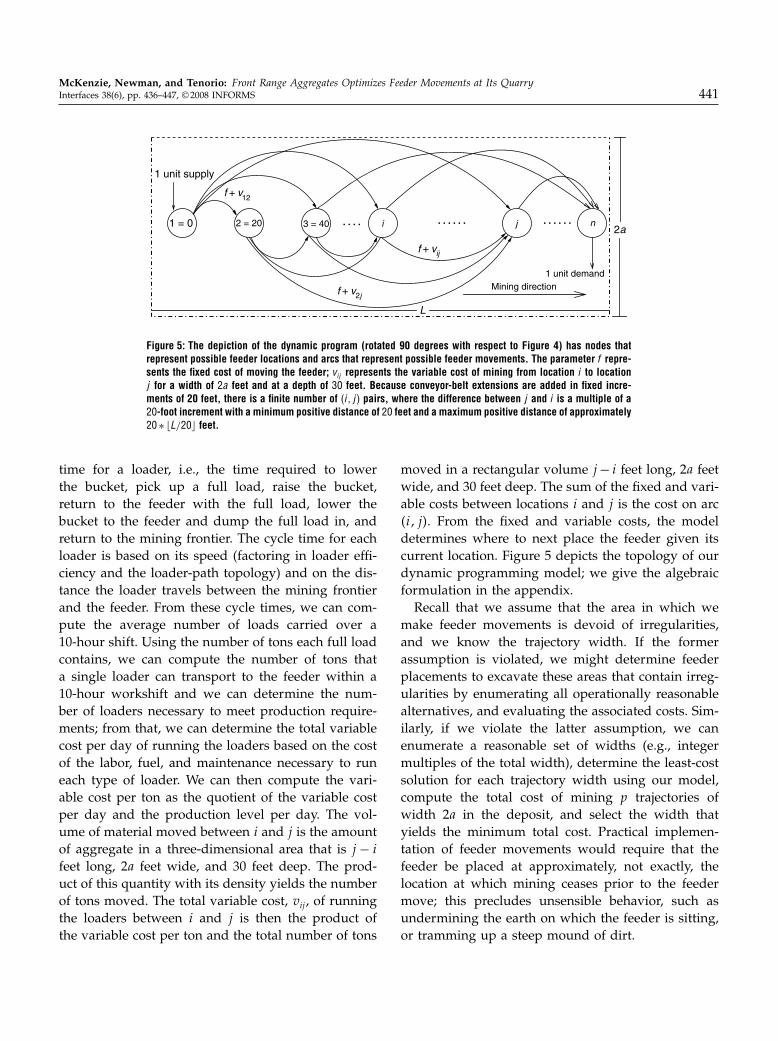
Figure 5: The depiction of the dynamic program (rotated 90 degrees with respect to Figure 4) has nodes thatrepresent possible feeder locations and arcs that represent possible feeder movements. The parameter f repre-sents the fixed cost of moving the feeder; vij represents the variable cost of mining from location i to locationj for a width of 2a feet and at a depth of 30 feet. Because conveyor-belt extensions are added in fixed incre-ments of 20 feet, there is a finite number of �i� j� pairs, where the difference between j and i is a multiple of a20-foot increment with a minimum positive distance of 20 feet and a maximum positive distance of approximately20 ∗ �L/20� feet.

time for a loader, i.e., the time required to lowerthe bucket, pick up a full load, raise the bucket,return to the feeder with the full load, lower thebucket to the feeder and dump the full load in, andreturn to the mining frontier. The cycle time for eachloader is based on its speed (factoring in loader effi-ciency and the loader-path topology) and on the dis-tance the loader travels between the mining frontierand the feeder. From these cycle times, we can com-pute the average number of loads carried over a10-hour shift. Using the number of tons each full loadcontains, we can compute the number of tons thata single loader can transport to the feeder within a10-hour workshift and we can determine the num-ber of loaders necessary to meet production require-ments; from that, we can determine the total variablecost per day of running the loaders based on the costof the labor, fuel, and maintenance necessary to runeach type of loader. We can then compute the vari-able cost per ton as the quotient of the variable costper day and the production level per day. The vol-ume of material moved between i and j is the amountof aggregate in a three-dimensional area that is j − i

feet long, 2a feet wide, and 30 feet deep. The prod-uct of this quantity with its density yields the numberof tons moved. The total variable cost, vij , of runningthe loaders between i and j is then the product ofthe variable cost per ton and the total number of tons

moved in a rectangular volume j − i feet long, 2a feetwide, and 30 feet deep. The sum of the fixed and vari-able costs between locations i and j is the cost on arc�i� j�. From the fixed and variable costs, the modeldetermines where to next place the feeder given itscurrent location. Figure 5 depicts the topology of ourdynamic programming model; we give the algebraicformulation in the appendix.Recall that we assume that the area in which we

make feeder movements is devoid of irregularities,and we know the trajectory width. If the formerassumption is violated, we might determine feederplacements to excavate these areas that contain irreg-ularities by enumerating all operationally reasonablealternatives, and evaluating the associated costs. Sim-ilarly, if we violate the latter assumption, we canenumerate a reasonable set of widths (e.g., integermultiples of the total width), determine the least-costsolution for each trajectory width using our model,compute the total cost of mining p trajectories ofwidth 2a in the deposit, and select the width thatyields the minimum total cost. Practical implemen-tation of feeder movements would require that thefeeder be placed at approximately, not exactly, thelocation at which mining ceases prior to the feedermove; this precludes unsensible behavior, such asundermining the earth on which the feeder is sitting,or tramming up a steep mound of dirt.


Dynamic programming models with a structuresimilar to ours have been successfully applied in in-dustries other than in mining, e.g., to minimize travelexpenses for federal employees (Huising et al. 2001),to determine the locations at which larvicide should besprayed (Solomon et al. 1992), and to schedule projects(Darrah 1984).

Results and ComparisonsThe Parkdale property consists of a deposit dividedinto two parts, each 1,200 feet wide. One deposit partis 1,800 feet long; the second is 1,000 feet long. Thesedeposit parts are free from irregularities. Our goalis to determine for each deposit part: (1) an opti-mal trajectory width from a set of candidate widths,and (2) optimal feeder moves along the trajectoryof that given width. Mine planners are interested inconsidering evenly spaced trajectory widths, i.e., tra-jectory widths that are multiples of 1,200 feet. There-fore, for each of the two deposit parts, we computethe optimal trajectory moves and the associated totalcost of mining the deposit for widths of 100, 200, 300,400, 600, and 1,200 feet. Because each network modelsolves quickly, the computational burden of solvingsix model instances for each deposit part is minimal.We implement the network as a shortest-path model

and process the results in a series of Excel worksheets.In the first worksheet, we accept cost information andthe desired trajectory width and compute arc costsbased on this information (appendix). We set up thesecond worksheet to handle the shortest-path networktopology of a deposit part of a given length; as inputs,it takes the costs in the first worksheet and computesthe optimal series of feeder movements along a trajec-tory of that given length for the width specified in thefirst worksheet. The underlying solver, invoked witha click of the “solve” button, is the Jensen NetworkSolver (coded by Paul Jensen at the University of Texasat Austin); it operates in a spreadsheet and can solvenetwork models as large as ours (i.e., models that con-tain 50–100 nodes and a few thousand arcs) in a mat-ter of seconds. The solver displays the solution andobjective function value in that second spreadsheet, inwhich we have created a macro, “capture flow,” thattranslates the arcs with a corresponding value of 1in the optimal solution to feeder locations and placesthese feeder moves in another worksheet.

Figure 6 shows the worksheet in which the net-work is solved as a shortest-path model. The rightside depicts representative cost information that iscollected on the first of the three worksheets. In theupper right corner, the spreadsheet shows the resultsof the “capture flow” macro, which translates theshortest-path solution into feeder locations and placesthe information in a third worksheet.For the 1,800-foot-length part of the deposit, optimal

feeder moves are spaced either 440 or 460 feet apart,and occur along a trajectory width of 1,200 feet. Specif-ically, the optimal mining plan is to place the feederat an initial location in the deposit that is 600 feetaway from its sides, excavate until the mining fron-tier reaches 440 feet from that initial location, movethe feeder approximately 440 feet, excavate until themining frontier reaches 900 feet from the initial loca-tion, move the feeder 460 feet, excavate until the min-ing frontier reaches 1,360 feet from the initial location,move the feeder to that point, and then excavate untilthe end of that part of the deposit. Optimal feedermoves for the 1,000-foot part of the deposit are similar:for a 1,200-foot-deposit width, move the feeder onceto 500 feet. In each case, no more than three loadersare needed.Without our model, mine planners would ignore

feeder movements until production requirementscould no longer be met using the existing fleet of load-ers. If we compute the costs associated with this sub-optimal policy using the trajectory widths that aremultiples of 1,200 feet, the lowest-cost widths for the1,800 and 1,000-foot-deposit parts are 1,200 and 600feet, respectively. For the 1,800-foot part of the deposit,the suboptimal policy would result in the feeder beingmoved once, at 1,260 feet (after which three load-ers could not meet production requirements). For the1,000-foot part of the deposit, no feeder move wouldbe necessary. For the 1,800-foot part of the deposit,the cost of the suboptimal policy is 14 percent higherthan the optimal solution; results for the 1,000-footpart of the deposit are similar; the cost of the subop-timal policy is 13 percent higher. The savings gainedfrom the use of our model apply to costs that con-stitute about half of the operating expenses at thequarry. (The other half is associated with plant oper-ation and train loading.) Note that these percentagesare actually lower bounds on the cost savings for two


Figure 6: We implement the network model and process the results using three Excel worksheets, which gathercost information (see the right side in this example), use this information and an underlying network solver (i.e.,the Jensen solver) to compute an optimal solution, and translate the optimal solution into a series of feedermovements (see the upper right corner).

reasons: (1) we assume that the mine would choosethe optimal trajectory width while determining feedermoves without our model, and (2) we do not considerthe detrimental effects of poor loader-maintenanceschedules, lack of coordination between feeder move-ments and scheduled downtime at the plant, and lowcustomer satisfaction because of late delivery resultingfrom suboptimal feeder movements.We began to develop the model at the start of 2004.

After working on it for a few months, we realizedthat a dynamic program solvable as a shortest-pathmodel would accurately capture the relevant deci-sions. In early 2005, we embedded our application ina spreadsheet; we transitioned the model to the minethat fall. While developing the model, two coauthors

met with the mine manager to verify the model’susefulness and validate the assumptions and calcula-tions therein. Upon its completion, one coauthor (andher research assistant) visited the mine site for sev-eral hours to install the software on the mine man-ager’s computer, explain the software to him, andgive him an instruction sheet. That manager, whohas been using the software since its installation inOctober 2005, now runs the model himself; he canmake changes to the number and type of operatingequipment and to the characteristics of the operatingequipment, such as costs and efficiency factors.Front Range Aggregates began to implement the

model recommendations mentioned above at itsParkdale property in January of 2006. Prior to the


implementation, the company used the authors’ rec-ommendations to mine its irregular areas. Althoughthese recommendations were not the result of theshortest-path solutions, they are relevant to the dis-cussion because: (1) they validated the cost structureswe use in our network model, and (2) they were doneusing our advice regarding the (small) enumerationprocedure we mention above. Subsequent to miningthe irregularities, the mine manager has been miningthe 1,000-foot part of the deposit, having placed thefeeder according to our recommendations. The modelis closely tracking the actual loader time requiredto feed the plant as the frontier moves away fromthe feeder. The manager plans to continue to movethe feeder according to our recommendations. Morethan one year later (as of this writing), the companyhas verified the cost savings we estimate, and hasrealized pit-haulage cost improvements approaching33 percent compared with the previous year’s lev-els. These savings are better than predicted becauseof both the conservative nature of our estimates andexternal factors. For example, the plant was able torun continuously because of, inter alia, favorable mar-ket conditions; additionally, the loaders experiencedno major mechanical problems. The company plans tocontinue to use the model where mine reserve char-acteristics allow its application.The usefulness of our dynamic program is evi-

dent from this cost comparison. Our model usesonly basic data and is relatively straightforward toimplement; the model does not require understandingof sophisticated mathematical modeling and yieldseasily executable and simple-to-understand policies.Finally, it produces solutions that improve the way inwhich aggregate quarries in general can plan feedermovements.

Appendix

Formulation

Indicesi� j = location of feeder along a straight-line trajectory.

n = last node = �L/20�.SetsN = nodes, i.e., feasible feeder locations (multiples of

20 feet from an initial location).

A = feasible adjacent feeder-location pairs (multiplesof 20 feet apart, terminal node > incident node).

Parametersf = fixed cost of moving feeder ($).

vij = variable cost of extracting and hauling all minedmaterial in the pit between location j and thefeeder located at i given a width of 2a feet anda depth of 30 feet ($).

Decision Variables

xij =

⎧⎪⎪⎪⎪⎪⎨⎪⎪⎪⎪⎪⎩

1 if the feeder is moved along its straight-line trajectory to location j , having lastbeen moved to location i,

0 otherwise�

Objectivemin

∑�i� j�∈A

�f + vij �xij �

Constraints

∑j

x1j = 1� (1)

∑i

xij =∑k

xjk ∀ j ∈ N� j �= 1�n� (2)

∑i

xin = 1� (3)

0≤ xij ≤ 1 ∀ �i� j� ∈ A� (4)

We minimize the total fixed costs of moving thefeeder and the variable extraction costs betweenfeeder movements. The constraint set forms sim-ple flow-balance requirements for a shortest-pathproblem, with a single unit supplied at the origin(node 1) and a single unit demanded at the destina-tion (node n).

Deriving the Average Haul Distance for a LoaderSuppose that we assume, without loss of generality,that the feeder is at the corner of an a × b rectangle(Figure A.1). We wish to compute the average hauldistance between the feeder and the mining frontier,where the mining frontier lies within the rectangle.We divide the rectangle into small squares, each oflength �, and approximate the distance between thefeeder and the mining frontier within one of the small


b = j– i(n of these)

aFeeder ... ΔΔ Δ Δ Δ

ΔΔΔ

Δ

...

•

•

•

•

•

•

•

••

•

(m of these)

Figure A.1: To derive the average haul distance for a loader between thefeeder and the mining frontier in an a × b rectangle, we divide the rect-angle into squares, and take the average distance from the feeder (at thebottom left corner) to the center of all squares inside the rectangle.

squares as the distance between the feeder and thecenter of said square. The average haul distance is thenthe average (two-way) distance between the feederand the center of all such squares within the a × b

rectangle. The lines in Figure A.1 comprised of bothdashes and dots show some representative distances.If we assume that the horizontal side of the rectan-

gle consists of m intervals of length �, and that thevertical side of the rectangle consists of n such inter-vals, then �i�+�/2� j�+�/2� for i = 0� � � � �m−1 andj = 0� � � � �n − 1 are the x and y coordinates, �xi� yj �,respectively, of the center of any small square withinthe a × b rectangle. The distance between the feederand the center of the �i� j�th square is

dij =√

�2�0�5+ i�2 + �2�0�5+ j�2�

and the haul distance D between the feeder and themining frontier in the a × b rectangle is the averagedistance across all such squares as the size of thesquares approaches zero:

D = limm�n→�

1nm

m−1∑i=0

n−1∑j=0

dij = 1ab

∫ a

0

∫ b

0

√x2 + y2 dx dy

=√

a2 + b2

3+ a2

6bln(

a + b + √a2 + b2

a − b + √a2 + b2

)

− b2

6aln(

b

a + √a2 + b2

)� (5)

a a

1 2... m 2... n

0

a /2 3a /2

1

Γ Γ Γ Δ Δ Δ.... ΔΓ....

Figure A.2: We show using a one-dimensional example how the approx-imation for the distance between the feeder and the mining frontierdepends on the geometry of the section.

Equation (5) follows from the definition of integral asa limit of Riemann sums. We can then calculate theintegral by dividing the rectangular domain into twoequal triangles and doing a polar coordinate transfor-mation in each triangle.

Geometry of the MineNote that the approximation for the distance betweenthe feeder and the mining frontier depends on thegeometry of the section, i.e., in our case, that we haveelected to use a rectangle for the shape of the minedarea, and squares for the subdivided areas, ratherthan other shapes. To see the importance of care-fully selecting a geometry that represents or closelyapproximates the actual loader movements, considerthe one-dimensional example in Figure A.2. We sep-arate a line segment of length 2a into two equal seg-ments, each of length a, and then subdivide one suchsegment into m subsegments and the other segmentinto n subsegments, where each of the first set of sub-segments has width � = a/m and each of the secondset has width � = a/n.Then, the average distance D�m�n� from the left

endpoint to the n + m segments along the line is

D�m�n� = 1m + n

( m∑i=1

i� +n∑

i=1

�a + i��

)

= 1m + n

��m�m + 1�/2+ an + �n�n + 1�/2

= a

m + n��m + 1�/2+ n + �n + 1�/2

= a

(12

+ 1+ 1/n

m/n + 1

)� (6)

If we let m = kn, where k is a positive integergreater than 1, and substitute this value for m into (6),


as n → �, we obtain

D�kn�n� = a

(12

+ 1+ 1/n

k + 1

)→ a

2

(k + 3k + 1

)∈ �a/2� a�

Hence, depending on the value for k, the average dis-tance from the left endpoint to any point on the linelies somewhere between halfway between the originand the midpoint of the line segment, and the mid-point of the line segment.If, however, we reverse the relationship between m

and n such that n = km, by the same logic, it followsthat the average distance from the left endpoint toanywhere on the line is

D�m�km� → a

2

(3k + 1k + 1

)∈ �a�3a/2

as m → �; thus, the average distance from the leftendpoint to any point on the line lies somewhere be-tween the midpoint of the line segment, and halfwaybetween the midpoint of the line segment and the endof the segment.Hence, we conclude that we cannot arbitrarily as-

sign dimensions to subsections of the mining fron-tier to approximate average loader travel distance.Instead, we must carefully choose a pattern thatclosely approximates actual loader movement.

AcknowledgmentsWe acknowledge the information and assistance that TomMaul, general manager of Front Range Aggregates, pro-vided. We also extend special thanks to Paul Jensen of theUniversity of Texas at Austin for supplying his solver freeof charge.

ReferencesAhuja, R., T. Magnanti, J. Orlin. 1993. Network Flows. Prentice Hall,

Englewood Cliffs, NJ.Akaike, A., K. Dagdelen. 1999. A strategic production method

for an open pit mine. 28th APCOM Sympos., Golden, CO,729–738.

Bolen, W. 2008. Mineral commodity summaries. Retrieved August 1,http://minerals.usgs.gov/minerals/pubs/commodity/aggregates.

Caccetta, L., S. Hill. 2003. An application of branch and cut to openpit mine scheduling. J. Global Optim. 27 349–365.

Carlyle, M., B. C. Eaves. 2001. Underground planning at StillwaterMining Company. Interfaces 31(4) 50–60.

Darrah, D. 1984. Project planning networks improve control. Build-ing 247(46) 91.

Erarslan, K., N. Celebi. 2001. A simulative model for optimum openpit design. CIM Bull. 94(1055) 59–68.

Fytas, K., J. Hadjigeorgiou, J. Collins. 1993. Production schedulingoptimization in open pit mines. Internat. J. Surface Mining Recla-mation 7 1–9.

Gove, D., W. Morgan. 1994. Optimizing truck-loader matching.Mining Engrg. 46(10) 1179–1185.

Hochbaum, D. 2001. A new-old algorithm for minimum-cut andmaximum-flow in closure graphs. Networks 37(4) 171–193.

Huising, J., H. Yamauchi, R. Zimmerman. 2001. Saving federaltravel dollars. Interfaces 31(5) 13–23.

Johnson, T. 1969. Optimum open-pit mine production scheduling.A. Weiss, ed. A Decade of Digital Computing in the Mineral Indus-try. AIME, New York, 539–561.

Johnson, T., K. Dagdelen, S. Ramazan. 2002. Open pit mine schedul-ing based on fundamental tree algorithm [sic]. 30th APCOMSympos., Phoenix, AZ, 147–159.

Kuchta, M., A. Newman, E. Topal. 2004. Implementing a pro-duction schedule at LKAB’s Kiruna Mine. Interfaces 34(2)124–134.

Lerchs, H., I. Grossmann. 1965. Optimum design of open pit mines.CIM Bull. 58(633) 47–54.

Norton, J. 1991. Three-dimensional surface modelling for mines andquarries. Quarry Management 18(9) 37–38.

Onur, A., P. Dowd. 1993. Open-pit optimization—Part 2: Produc-tion scheduling and inclusion of roadways. Trans. Inst. MiningMetallurgy Sect. A Mining Indust. 102 105–113.

Ramazan, S., R. Dimitrakopoulos. 2004. Traditional and new MIPmodels for production scheduling with in-situ grade variabil-ity. Internat. J. Surface Mining 18(2) 85–98.

Sarin, S., J. West-Hansen. 2005. The long-term mine productionscheduling problem. IIE Trans. 37(2) 109–121.

Sevim, H., D. Lei. 1998. The problem of production planning inopen pit mines. INFOR 36(1–2) 1–12.

Solomon, M., A. Chalifour, J. Desrosiers, J. Boisvert. 1992. An appli-cation of vehicle-routing methodology to large-scale larvicidecontrol programs. Interfaces 22(3) 88–99.

Underwood, R., B. Tolwinski. 1998. A mathematical programmingviewpoint for solving the ultimate pit problem. Eur. J. Oper.Res. 107 96–107.

Wilke, F., T. Reimer. 1977. Optimizing the short term produc-tion schedule for an open pit iron ore mining operation. 15thAPCOM Sympos., Brisbane, Australia, 425–433.

Willet, J. 2008. Mineral commodity summaries. Retrieved August 1,http://minerals.usgs.gov/minerals/pubs/commodity/aggregates.

Thomas M. Maul, General Manager, Front RangeAggregates, LLC, 3655 Outwest Drive, ColoradoSprings, CO 80910, writes: “Planning of pit feedermovements in the aggregates industry is rarely per-formed using sophisticated techniques. Traditionally,mine managers have tended to defer the cost andeffort of this task until absolutely necessary, i.e., untilproduction requirements can no longer be met withfull utilization of the existing mobile equipment fleet.Contributing to the problem is the fact that manyaggregate mines exist on a scale that does not justify


a management “team,” many having a single personmanaging the entire mine. Such a person does nothave a great deal of time to perform lengthy optimiza-tion analyses, and so the planning of unit operationsis driven by the desire to meet short-term objectives;not long term performance.“The spreadsheet model described in this paper

allows mine planners (managers) to quickly enter rel-evant operating cost data, and describe pit dimen-sions. The optimization model then uses this data tocompute a sequence of pit feeder movements whichminimizes pit operating costs over the life of the pit.Changing the data inputs is relatively simple and doesnot take much time, making the model practicallyapplicable to most equipment and pit configurationsfound in typical alluvial aggregate mining operations.

“Front Range Aggregates (FRA) implemented themodel recommendations for pit feeder placement atour Parkdale aggregates mine in January of 2006, andto date (approximately 12 months of operation) haverealized pit haulage cost improvements approaching33% compared to 2005 levels. We have not yet com-pleted one full cycle of pit feeder movements, butoperational characteristics of the pit are closely con-forming to those predicted in the model at this point,and we expect full cycle results to be consistent withthose predicted by the model over the life of the mine,barring unforeseen external influences.“FRA will continue to utilize the model where mine

reserve characteristics allow its application, and weexpect it to be a useful tool for our operation staff inour efforts to optimize operational performance.”

front range aggregates optimizes feeder movements …inside.mines.edu/~anewman/mckenzieetal.pdf ·...

Documents