From Weber to Kafka: Political Activism and theEmergence of an Inefficient Bureaucracy

Gabriele Gratton,∗ Luigi Guiso,†

Claudio Michelacci‡ and Massimo Morelli§

July 29, 2015- Preliminary

Abstract

This paper models the relationship between legislative activity and bureaucracy.

We characterize the Weberian Steady State and the Kafkian Steady State, and we show

what type of shocks can lead to a transition from a good Weberian economy to a

Kafkian one. The main message is that excessive political activism (frequent reforms

and new laws, due for example to political instability) reduce bureaucratic efficiency,

and this in turn creates more incentives for incompetent politicians to further increase

their legislative activities, which bring to further inefficiency.

1 Introduction“Corruptissima re publica plurimae leges"1

Cornelius Tacitus, Annals, Book III, 27

With the term "bureaucracy" we usually refer to the body of non-elective governmentofficials who provide important services to individuals like regulation, certification, en-forcement and implementation of laws. In other words, politicians "choose" (policies orlaws, hence think of legislative as well as executive branch) and bureaucrats are called to"implement".

∗UNSW, email: g.gratton@unsw.edu.au.†EIEF and CEPR, email: luigi.guiso@tin.it‡EIEF and CEPR, email:c.michelacci1968@gmail.com§Bocconi University and Igier, email: massimo.morelli@unibocconi.it1Translation: When the republic is at its most corrupt the laws are most numerous

1

Broadly speaking, we can say that there are two main views about bureaucracy. Onthe one hand, the German sociologist Max Weber argued that bureaucracy constitutes themost efficient and rational way in which human activity can be organized. He argued thathaving systematic processes and organized hierarchies is necessary to maintain order,maximize efficiency and eliminate favoritism in economies.2 The second view, whichis dominant these days, is that bureaucracies sometimes become too complex, and tooinflexible. The dehumanizing effects of excessive bureaucracy were a major theme inthe work of Franz Kafka in his two classic unfinished novels titled “Der Process” (theTrial) (published in 1925) and “Das Schloss” (the Castle) (published in 1926). A Kafkianbureaucracy is marked by a senseless disorienting, often menacing complexity, whichultimately leads to a country’s stagnation.

This paper offers a theoretical explanation and an empirical investigation of the maincauses of a transition from a Weberian bureaucracy to an inefficient Kafkian one. More-over, we do so by focusing primarily on the role of political instability and political ac-tivism by legislators, rather than zooming on the bureaucracy organization as a set ofspecific agencies with different career concerns.3

In the 19th century, the bureaucracy of the Habsburg Monarchy was taken as an exam-ple of bureaucratic efficiency (see e.g. Becker, Boeckh, Hainz and Woessmann, forthcom-ing). But at a point the system collapsed.4 What could be the reason of this sharp transfor-mation happening just before Kafka’s books? The answer that we will provide will referto a set of political instability shocks reported by historians: in the Austro-Hungarianempire ethnic conflicts became open political confrontations in that period, and substan-tial nationalistic pressures from more than 12 different ethnicities and tensions betweendifferent ideologies (liberalism versus ancient regime) gave rise to a big jump in politicalinstability. As a result the number of political parties exploded—for example there were50 political parties participating to the election of 1911—and the number of MPs in theLower house increased substantially—from 203 to 516 over the 1867-1918 period. Overthe same period, Austria had 29 Ministers Presidents.

Can political instability be the source of the transition from Weber to Kafka? This pa-

2Even Weber saw unfettered bureaucracy as a threat to individual freedom, in which an increase in thebureaucratization of human life cantrap individuals in an "iron cage" of rule-based, rational control, but hisoverall evaluation remained one of necessity and efficiency.

3For an overview of the large literature on the agency problems in the construction of a bureaucracy,see Gailmard and Patty (2012).

4The payment of a simple tax in Wien at the beginning of the 20th century required the contributionof 27 public officials; the cost of collecting taxes in Dalmacia was superior to the amount of tax revenuecollected; in 1903, the English Embassy had to wait 10 months before receiving information on how to paytaxes to import Canadian Whiskey (MacMillan, 2013).

2

per says definitely yes. We propose a dynamic model in which political activism in theform of multiplication of laws and reforms can affect bureaucratic efficiency and we char-acterize the consequent politics bureaucracy nexus. We will see that (1) starting from aWeberian steady state characterized by high bureaucratic efficiency there exist shocks interms of political instability and/or need of reforms that could increase legislative ac-tivism enough to make bureaucracy collapse and converge towards a Kafkian steadystate; (2) moreover, even when an increase in reforms and new laws comes from compe-tent technocrats, the effect on the deterioration of bureaucracy is still present, and couldinduce further bad reforms by bad politicians going forward; (3) the probability of badreforms is decreasing in the efficiency of bureaucracy and the length of a legislature.

Bureaucracy is more powerful and/or more inefficient when the amount of laws in-crease. In turn, we emphasize that whenever bureaucracy is more inefficient, politiciansare more active in passing new laws. This two-way connection leads naturally to the pos-sibility of multiple equilibria in the short run and multiple steady states in the dynamicanalysis.

There could be multiple mechanisms underpinning the finding that a more inefficientbureaucracy generates greater legislative activism: one mechanism was already empha-sized by Tacito: when bureaucracy is corrupt, politicians introduce new laws useful toattack political enemies, to protect vested interests and to appropriate rents in the econ-omy. Another mechanism is trivial: politicians introduce more laws to simply reform theinefficient powerful bureaucracy. The third mechanism, which has been overlooked andis key in our analysis, is the following: An essential feature of bureaucracy in advancedeconomies is to provide a high quality monitoring of political activity. When bureaucracyis powerful (or inefficient), politicians are inaccurately monitored and politicians becometempted to inundate the system with a tsunami of laws to build up their reputation ofskillful reformers. This third mechanism that we emphasize has the testable implicationthat the increase of reform incentives when bureaucracy is inefficient should come pri-marily from low quality politicians, and this is a micro test that we will undertake.

Model characterization Our model is characterized by two schedules, that can be bothdepicted in the h-1/α space (h in x-axis and 1/α in y-axis). Think of h as a measure ofpolitical activism or amount of regulation in the economy. Think that 1/α measures the in-efficiency or the Power of bureaucracy. The latter is one interpretation for why α decreaseswhen there are more laws in the system (when h goes up). Now the steady state of theeconomy is characterized by two lines. One is a technological constraint, that we callthe Power of bureaucracy line (the PB-line thereafter). This line says that the higher ish, the less efficient (or more powerful) is bureaucracy (higher 1/α). Given our assump-

3

tions, this is a stepwise increasing function with just one step corresponding to hw. Butgenerally we should think that the PB line is positively sloped: bureaucracy is more pow-erful and/or more inefficient when the amount of regulation (laws, political activism)increases. The second line is instead a relation that says that whenever bureaucracy ismore inefficient, politicians are more active in passing new laws. This establishes (an-other) positively sloped relation between 1/α and h. We call this the Tacito line (T-linethereafter). There are several reasons that explain why this line is positively sloped. Oneis emphasized by Tacito: when bureaucracy is corrupted, politicians introduce new lawsuseful to attack political enemies, to protect vested interests and to appropriate rents inthe economy. Another is trivial: politicians introduce more laws to simply reform theinefficient powerful bureaucracy. We emphasize another one. An essential feature ofbureaucracy in advanced economies is to provide a high quality monitoring of politicalactivity. When bureaucracy is powerful (or inefficient), politicians are unaccurately mon-itored and politicians become tempted to inundate the system with a tsunami of laws tobuild up their reputation of skill-full reformers. This increases the amount of regulationin the system. Since both the T-line and the PB-line are positively sloped, multiple equi-libria are possible (Weber vs Kafka equilibria). We emphasize that some parameters shiftthe T-line (while leaving the PB-line unchanged), and in particular we emphasize that po-litical instability makes the T-line flatter and makes more likely that the Kafkian equilib-rium emerges. Luigi has provided some evidence in favor of the existence of the PB line:there is a positively sloped relation between amount of regulation in the economy andthe power of bureaucracy. The former is measured by the number of procedures neededto start-up businesses, to register property, to get electricity and to obtain a constructionpermit (using the Doing Business World Bank Dataset). The latter is measured by howopaque and little transparent is bureaucracy in the country. We are trying to show thatcountries that have experienced higher past political instability (short lived governments)are more likely to end up in a situation where bureaucracy is inefficient and regulation ispervasive. END

A few notes on the relationship with the literature are in order. Our results are ob-tained when thinking about (and modeling) bureaucracy as complementary rather thansubstitute to politics. Maskin and Tirole (2004), Alesina and Tabellini (2007; 2008) askunder what conditions it is better to delegate choices to a bureaucracy and under whatconditions it is instead better to let elected officials make the policy calls. We believeinstead that most policies require both a legislative or executive decision by politiciansand necessary procedures of enforcement, implementation and alike by the non-electivebureaucracy. Castanheira, Herrera, and Ting (2015) start from the same premise about

4

complementarity of politicians and bureaucrats in policy making, and also start from theempirical observation of a negative correlation between length of legislatures and bu-reaucratic performance, but focus the analysis on the role of ideology and on the choicebetween patronage system and civil service. On the other hand, we assume a simple formof bureaucracy, of the civil service type (appointed for life) and avoid dealing with ideol-ogy altogether, focusing instead on the politicians’ incentives to legislate even when thereis no need of reforms.

Nath (2015) provides evidence that electoral competition affects negatively bureau-cratic performance, but the mechanism she focuses on relates to the internal functioningof the bureaucracy rather than on the legislators’ incentives. She emphasizes that incum-bents with longer tenure can use sort of dynamic contracts, rewarding bureaucrats withfuture payoffs or threatening implicitly to change their jobs in case of delay. Given thatour theoretical analysis focuses on political activism, we provide empirical evidence notonly about the direct consequences of more legislative activism on bureaucratic perfor-mance, but also on the feedback effect, namely on the greater incentives to make reformsby bad politicians when the expected duration of office is low and bureaucracy is alreadyslow.

Persson, Tabellini, and Trebbi (2003) explore the effects of electoral institutions on cor-ruption, but do not address the effects of electoral turnover.

2 Model

2.1 Setup

We consider an infinitely lived economy where the production of output requires publiccapital,5 which is jointly produced by politicians and bureaucracy.

Time is continuous and indexed by τ ≥ 0.

Politicians The economy is ran by a continuum of ministries indexed over the unit in-terval, i ∈ [0, 1]. Ministry i is ran by a politician who remains in power for one legisla-ture.6 The duration of each legislature equals ` ≥ ` > 0.7 Legislatures are indexed by

5We intend public capital to capture the whole body of public regulations, organizations, and infras-tructures that facilitate production and trade.

6See Appendix B for a robustness exercise looking at a two-period model in which politicians can bereelected.

7The lower bound ` is determined by technological constraints on the functioning of ministries and theelectoral system.

5

t = 1, 2, . . . , where legislature t starts at date τt ≡ (t− 1) `.At the beginning of legislature t, a new politician is elected to run each ministry. For

simplicity, we refer to the politician elected in ministry i in legislature t as “minister it.”Minister it privately knows her type θit ∈ {0, 1}. If θit = 1, then minister it is competent.Otherwise, she is incompetent. Each minister is competent with identical probability π.

At the start of her mandate, minister it is endowed with a reform. With probabil-ity pθit, the reform is good; otherwise it is bad. The minister then immediately chooseswhether to start the reform.8 Notice that only competent politicians can start good re-forms, but all politicians can start bad reforms. The probability p is meant to capture theeconomy’s need for reforms.

Bureaucracy Reforms are completed by the bureaucracy. Reforms started at beginningof legislature t are completed at Poisson arrival rate αt = α (ht), where ht is the stockof incomplete reforms inherited from the previous legislature. Notice that αt is constantover legislature t. The value αt measures the efficiency of the bureaucracy during legislaturet.

The function α is decreasing in ht: a higher stock of uncompleted reforms reduces thecompletion rate of reforms. There are several reasons why the efficiency of bureaucracyis decreasing in the amount of political activism. One could be technological: more re-forms congestion the bureaucratic apparatus that becomes inefficient due to its limitedability to handle an excessive stock of information. But we can also think that more polit-ical reforms ht give more power to bureaucracy and a more powerful bureaucracy becomesopaque, complex and obsessed with formalism. This is the natural reaction of an institu-tion that builds up complexity to preserve its power. One way or the other, more politicalactivism makes bureaucracy more inefficient which explains why the function α (ht) isdecreasing in ht. For simplicity we omit modeling the instinct of preservation and powerbuilding of bureaucracies, because, in practice, the exact reason for why bureaucratic effi-ciency falls with political activism is irrelevant to explain why countries might experiencea transition from a Weberian to a Kafkian bureaucracy. For simplicity we assume that αt

can assume only two values, α and α, with 0 < α < α. The function α : R+ → {α, α} canthen be expressed as

α (ht) =

α if ht ≤ hK

,

α if ht > hK (1)

8The assumption that reforms must be started at the beginning of the legislature greatly simplify theanalysis by eliminating unintuitive (and not robust) equilibria in which good reforms are delayed for repu-tational concerns.

6

where hK

is the Kafkian threshold of hanging reforms beyond which bureaucratic effi-ciency collapses—i.e., the completion rate of reforms falls from α to α. We refer to a bu-reaucracy with αt = α as Weberian and to a bureaucracy with αt = α as Kafkian.

The Economy and Welfare The economy is populated by a representative householdwith zero discount rate, no access to savings, and income at time τ given by

Akτ (2)

where kτ > 0 is the stock of public capital at τ and A > 0. Aggregate welfare is thereforegiven by average-over-time long-run aggregate income.

Once completed, a good reform yields q units of public capital. Bad reforms produceno economic outcomes, even when completed. Competent ministers maintain their gooduncompleted reforms up-to-date during their mandate, but after their mandate expires,good (either completed or uncompleted) reforms turn into bad at Poisson arrival rate ν.The idea is that competent politicians have the skill of keeping alive their good reformsby adapting their reforms to the changing economic environment. After the mandate ofthe politician expires, reforms are out of the control of the politician who proposed themand reforms depreciate at rate ν. The idea is that reforms are good just in a determinedeconomic context. As the economy evolves they eventually get obsolete and useless.

Public Reputation At the end of each legislature t and for each ministry i ∈ [0, 1], thepublic observes whether the incumbent politician has started a reform, whether the re-form has been completed and if so the amount of capital services it has produced. Wedenote by ρit the beliefs of the public about minister it being competent at the end oflegislature t—at time τt + `.

Politicians in power have reputational concerns. Minister it’s payoff is given by

Et [φρit − γθitI (ρit = 0)] (3)

where I denotes the indicator function while Et is the expectation operator conditionalon the information available at the start of legislature t. Here φ > 0 measures the pri-vate value of reputation to politicians while γ is the moral cost suffered by a competentpolitician, θ = 1, if the public believes she is incompetent (ρit = 0). There are severalreasons why reputation matters to politicians. For example reputation could have valuein the private market and politician with higher reputation can extract higher rents in the

7

market once their mandate expires.9 In this interpretations φ just measures the marketvalue of reputation. The specification in (3) is also consistent with the idea that politiciansare motivated by re-election concerns,10 provided that re-election probabilities are strictlyincreasing in the reputation of politicians. In either interpretation the value of reputa-tion φ would be endogenous, but since φ does not play any specific role in the analysisbelow—of course provided it remains strictly positive, φ > 0—we omit characterizingthe equilibrium value of reputation.11

We intepret γ as a moral cost. Alternatively, it can be thought of as a competent politi-cian’s cost of losing access to a labor market in which competence is revealed with strictlypositive probability.12 In the analysis below we assume that the moral cost γ is highenough so that the following assumption holds:

Assumption 1. Assume that γ > φ.

Assumption 1 guarantees that competent politicians start a reform only if they havethe opportunity of a good reform.

Given Assumption 1, the only strategic choice in the model is the incompetent politi-cians’ choice of whether to start a reform. We denote by σt ≡ σit (αt) the probability thatminister it starts a reform when the the level of efficiency of the bureaucracy equals αt.The focus on symmetric and stationary strategies is without loss of generality.

We focus on perfect Bayesian equilibria with neutral off-equilibrium beliefs:

Definition 1. An equilibrium is a strategy σ and belief ρit, ∀i ∈ [0, 1] , t ∈N such that

σt = arg maxσ∈[0,1]

Et [φρit − γθitI (ρit = 0)]

and ρit is derived by Bayes’ rule whenever possible, and ρit = π otherwise.

9See e.g. Mattozzi and Merlo (2008).10An implicit assumption if we interpreted φ as value of reelection is that being a good politician today

does not increase the probability of being a competent politician tomorrow over π (for example becauseskills in time of crisis may be uncorrelated with skills in time of boom), because otherwise the public wouldalways reelect the same politician revealed to be competent once, and hence the fix probability π acrossperiods would be an inconsistent assumption. See appendix B for a robustness exercise looking at a two-period model in which indeed π may depend on the revealed information on incumbent when reelected.

11It is important to stress that the gains from reputation to politicians should be interpreted as a transferfrom households to politicians, so aggregate welfare at time τ is still given by (2).

12Details are available upon request.

8

3 Dynamics

To better understand the analysis, it is useful to separately study some non-strategic dy-namics of the model.

Recall that the level of efficiency of the bureacracy αt depends on the stock of unreal-ized reforms inherited by legislature t from all previous legislatures, ht (i.e. ht is the stockof hanging reforms just before time τt). For any t = 1, 2, . . . , ht evolves according to thefollowing first order difference equation:

ht = e−αt−1` (ht−1 + rt−1) (4)

This says that the stock of unrealized reforms immediately before the beginning of legis-lature t is equal to the fraction e−αt−1` of reforms present at the beginning of the t− 1thlegislature that have not come to completion. The amount of uncompleted reforms at thebeginning of the t− 1th legislature is equal to the sum of uncompleted reforms inheritedfrom all the legislatures prior to the t− 1th, equal to ht−1, plus the mass of newly startedreforms in the t− 1th legislature

rt−1 = πp + (1− π) σt−1 (5)

which is equal to the sum of the good reforms started by competent politicians πp plusthe mass of bad reforms started by incompetent politicians, equal to (1− π) σt−1. The lawof motion in (4) implies that the steady state number of uncompleted reforms at the startof each legislature is equal to ht = ht−1 = h∗:

Lemma 1. The steady state stock of uncompleted reforms at the start of each legislature is givenby

h∗ =r∗

eα∗` − 1(6)

where r∗ = πp+ (1− π) σ∗ denotes the steady state flow of new reforms started at the beginningof each legislature where σ∗ denotes the steady state probability that an incompetent politicianstarts a reform.

We are interested in determining aggregate welfare. Recall that aggregate welfareis monotonically increasing in capital, which is produced when good reforms are com-pleted. For any τ ∈ [τt, τt + `) we denote by gτ the stock of good uncompleted reformsinherited from previous legislature at time τ and by nτ the stock at time τ of uncompletedgood reforms which have been newly started in the current legislature. The stock of goodold reforms during the t-th legislature gτ decreases at rate αt + ν, because some of them

9

are completed at Poisson arrival rate αt while some get obsolete and bad at Poisson ar-rival rate ν. This implies that for any τ ∈ [τt, τt + `) the stock of good uncompleted oldreforms is equal to

gτ = e−(αt+ν)(τ−τt)gt (7)

where gt is the stock of good reforms at the beginning of legislature t. The amount ofnewly started uncompleted good reforms at time τ is equal to

nτ = e−αt(τ−τt)πp. (8)

Therefore,gt = e−(αt−1+ν)`gt−1 + e−αt−1`πp. (9)

Finally, for any τ ∈ [τt, τt + `), we have that the stock of capital evolves as

dkτ

dτ= qαt (gτ + nτ)− νkτ. (10)

We can now substitute (8) and (7) into (10) to obtain that ∀τ ∈ [τt, τt + `)

dkτ

dτ= qαte−αt(τ−τt)

[e−ν(τ−τt)gt + πp

]− νkτ (11)

Notice that (9) and (11) represent a recursive system: given gt and αt, use (11) to obtain

kτ = kτt e−ν(τ−τt) +

qαtπp(ν− αt)

[e−αt(τ−τt) − e−ν(τ−τt)

]+ qgt

[e−ν(τ−τt) − e−(αt+ν)(τ−τt)

](12)

where kτt denotes the capital stock at the beginning of legislature t. By evaluating thisexpression at τt+1 = τt + ` and after remembering that by continuity we have kt = kτt , wecan also write the following first order difference equation in the beginning of legislaturecapital stock kt :

kt+1 = e−ν`kt +qαtπp(ν− αt)

[e−αt` − e−ν`

]+ qgt

[e−ν` − e−(αt+ν)`

], (13)

Now we can use (9) to conclude that in steady state gt is equal to

g∗ =e−α∗`πp

1− e−(α∗+ν)`(14)

where α∗ denotes the steady state completion rate of reforms. We can now use the expres-sion for g∗ in (14) to replace gt in (13). After imposing that the steady state capital stock

10

at the beginning of legislature should satisfy kt = kt−1 = k∗ we obtain that

k∗ =qπp

1− e−ν`

α∗(

e−α∗` − e−ν`)

ν− α∗+

1− e−α∗`

e(α∗+ν)` − 1

. (15)

We can now calculate the steady state average-over-time capital sock:

Lemma 2. The steady state average-over-time capital stock is equal to

k∗=

´ `0 kτt+sds

`=

qπpν`

(1− νe−α∗`

α∗ + ν

). (16)

Proposition 1. Aggregate welfare is monotonically increasing in the steady state completion rateof reforms α∗.

Even if agents have a zero discount rate, a higher α∗ increases welfare because higherα∗ means that good reforms yields greater expected income, because a higher α∗ reducesthe risk that good reforms becomes obsolete before they are completed, which would leadto no output gains.

3.1 First best

With no asymmetric information, there are no reputation concerns because the type ofpoliticians is perfectly observable. So (i) incompetent politicians do not start any reformsand (ii) competent politicians start reforms only if they have the opportunity for a goodreform, which occurs with probability p at the start of each legislature. As a result, andgiven Assumption 2, we have that the long-run completion rate of reforms α∗ is equalto α. This implies that aggregate welfare as measured by k

∗in (16) is maximum. We

can also calculate what it would be the optimal duration of a legislature in this first bestenvironment. We can derive k

∗in (16) with respect to ` to obtain

∂k∗

∂`= −qπp

ν`2

[1− ν

ν + α(1 + α`) e−α`

]< 0

This derivative is negative because the function (1 + α`) e−α` is strictly decreasing in `

for any ` ≥ 0 and it is smaller than one. Figure 1 plots the profile of the average capitalstock in the economy k

∗as a function of the duration of the legislature ` at the Weberian

completion rate of reforms α and at the Kafkian one α.

11

ℓ

𝑘 ∗

ℓ∗ ℓ∗∗

•

•

•

𝐹𝐵

𝐴

𝐵

𝑘 ∗(𝛼 )

ℓ

𝑘 ∗(α)

Figure 1: Welfare and the duration of the legislature

Since k∗

is strictly decreasing in `, we have that the optimal duration of a legislature isthe lowest as possible, `FB = `, which corresponds to point FB in Figure 1. This is becausea shorter legislature allows to maximize the flows of good reforms into the system. Wecan summarize all these considerations by stating the following proposition:

Proposition 2. Under Assumption 2, in the economy with no asymmetric information, all com-petent politicians with a good reform, and only them, start a reform. This leads to a first bestaverage-over time capital stock equal to

k∗FB ≡

qπpν`

(1− νe−α`

α + ν

).

The length of the legislature which maximizes steady state welfare in the economy with no asym-metric information is `FB = `, where ` is the minimal feasible duration of a legislature.

4 Political Equilibrium

We now turn to the analysis of the equilibrium of the model with reputational concernsdue to asymmetric information. We start by characterizing the optimal strategy of an

12

incompetent politician.By Assumption 1, competent politicians do not start bad reforms. We also know that

competent politicians always start good reforms whenever an opportunity arrives. Noticethat if σt = 0 (all bad politicians never start reforms), the reputation at the end of themandate of a politician who has not started a reform is equal to ρ ≡ π(1−p)

1−πp . This is simplythe ratio between the probability that the politician is good and and he did not have agood reform—which happens with probability π (1− p)—over the probability that nogood reform was available to the politician—which happens with probability 1− πp. Wecan extend the same logic for an arbitrary value of σt. By Bayes’ rule, we then obtain

ρit =

ρn

t ≡π(1−p)

π(1−p)+(1−π)(1−σt)if no reform is started

ρyt ≡

πpπp+(1−π)σt

if a reform is started and is not completed

θ if a reform is started and is completed.

(17)

Here ρnt is simply the ratio between the probability that the politician is competent and

and he did not have a good reform, over the probability that no reform was started (ei-ther because the politician is competent and did not have any good reform to pursue orbecause the politician is incompetent and decided not to start any reform). By a similarlogic we can calculate the reputation of a politician in case a reform is started but did notcome to realization during the legislature, which is denoted by ρ

yt . By Bayes’ rule, ρ

yt is the

ratio between the probability that the politician is competent and and he started a reform,over the probability that a reform was started by either a competent or an incompetentpolitician.

Given (3), the incompetent politician chooses σt so as to maximize his expected repu-tation at the end of the mandate. If an incompetent politician does not start any reformhis reputation at the end of the legislature is equal to ρn

t while if she starts a reform, hisexpected reputation at the end of her legislature is equal to e−αt`ρ

yt , where e−αt` is the

probability that the reform was not completed over the mandate of the politician. Noticethat it is never optimal to choose σt = 1, because under σt = 1 and given (17) we haveρ

yt e−αt` < ρn

t , which immediately implies a contradiction. The incompetent politicianchooses σt = 0 if ρ

yt e−αt` < ρn

t , which is equivalent to

αt` > − ln(

ρ)

. (18)

13

Otherwise, σt ∈ (0, 1) is determined by the indifference condition

e−αt`ρyt = ρn

t (19)

Notice that (18) together with (19) implies that σt is continuous in any change of parameters.We can then summarize these considerations by stating the following proposition, fullyproved in the Appendix, that characterizes the optimal strategy of an incompetent politi-cian:

Proposition 3. The equilibrium probability that an incompetent politician starts a reform equals

σt ≡ σ (αt) =

0, if αt` > − ln

(ρ)

p− p(1−p)(1−e−αt`)(1−π)[1−p(1−e−αt`)]

, otherwise.(20)

The probability σt has the following properties: (i) it is smaller than p; (ii) it is increasing in theneed of reforms of the country as measured by p; while (iii) it is decreasing in the duration of thelegislature `, in the probability that a politician is competent π, and the completion rate of reformsαt. Finally we have (iv) that the difference p − σt is (weakly) increasing in the duration of thelegislature ` and the completion rate of reforms αt, while it is decreasing in the need of reforms ofthe country as measured by p.

5 Equilibirum Dynamics

We turn now to the analysis of the long run steady-state behavior. We say that a steady-state is Weberian if in it the bureacuracy is Weberian and politicians only start good re-forms. In contrast, a steady-state is Kafkian if in it the bureaucracy is Kafkian and politi-cians start bad reforms with strictly positive probability. Our ultimate goal is to under-stand what causes a Weberian economy to become Kafkian. In order to do so, we imposeupon the model parameters sufficient and necessary conditions for the existence of a We-berian steady state.

Assumption 2. The Weberian completion rate reforms α is such that

πpeα` − 1

≤ hK

and α` ≥ − ln(

ρ)

.

14

To see why Assumption 2 guarantees the existence of a Weberian steady state for any` ≥ `, notice that for a Weberian steady state to exist we need to satisfy two conditions: (i)that a Weberian economy remains Weberian if only good reforms are started, and (ii) thatin equilibrium only good reforms are started in a Weberian economy. Recall that if onlygood reforms are started, then the steady state stock of hanging reforms at the beginningof a new legislature h∗ equals

πpeα` − 1

≤ πpeα` − 1

≤ hK

.

Thus, the first condition in Assumption 2 says that if only good reforms are started when-ever the bureaucracy is Weberian, then the bureacuracy remains Weberian. From Propo-sition (3), it is easy to see that the second condition in Assumption 2 says that, in equilib-rium, when the bureaucracy is Weberian, only good reforms are started.

Notice that Assumption 2 also guarantees that all steady states are either Weberian orKafkian.

5.1 The emergence of a Kafkian equilibrium

An important implication of Proposition 3 is that an inefficient bureaucracy (lower αt)gives incompetent politicians the incentive to start bad reforms. This effect will be moreimportant the shorter the legislature `. An efficient bureaucracy allows the public to eval-uate the activity of politicians. But when bureaucracy is inefficient, the public becomesunable to evaluate whether reforms are successful and as a result incompetent politiciansinundate the system with a "tsunami of reforms", which will eventually cause a collapseof the bureaucratic apparatus and the emergence of a Kafkian bureaucracy. We now betterinvestigate this mechanism.

The law of motion of the stock of uncompleted reforms ht is given in (4). The mass ofreforms introduced in the system at the start of legislature t is equal to rt in (5), which,given Proposition (3), can be expressed as equal to

rt =

πp, if αt` > ln(

ρ)

pp+(1−p)eαt`

, otherwise.(21)

Now notice that∂ ln

(ρ)

∂p=

p (1− π)

(1− πp) (1− p)> 0

15

while∂ ln

(ρ)

∂π= − 1

π (1− πp)< 0

which says that incompetent politicians are more likely to start a reform when p is highor π is low. It is interesting to notice that (21) implies that when σt > 0 the flow of newreforms introduced in the system is independent of π. The steady state mass of uncom-pleted reforms at the start of each legislature is given in (6), with r∗ satisfying (21). Afterusing Proposition 3 and (21) we can now state the following Proposition:

Proposition 4. There always exists a Weberian steady-state with

hW ≡ πpeα` − 1

≤ hK

. (22)

A Kafkian steady state exists if and only if both

α` < ln(

1− πpπ (1− p)

)(23)

andhK ≡ p[

p + (1− p) eα`] (

eα` − 1) > h

K(24)

The Kafkian steady-state is more likely to exist when (i) the need for reforms is high (p high), (ii)legislatures are short (` low), (iii) there are few competent politicians (π low), and (iv) a Kafkianbureaucracy is highly inefficient (α low).

High p, low ` and low α make more likely that both conditions (23) and (24) are sat-isfied, while low π makes more likely that the Kafkian equilibrium can arise by makingcondition (23) more likely to be satisfied.

In Figure 2 we characterize the law of motion of ht in (4) as a function of ht−1, whenboth the Weberian and the Kafkian equilibrium can arise, so that both (23) and (24) hold.Notice that (4) implies that ht is always flatter than the 45 degree line. The Weberianequilibrium corresponds to point W in Figure 2, the Kafkian equilibrium to point K.

5.2 Transitory shocks

A key feature of the model is that, when (23) and (24) hold, transitory shocks can leadthe economy to a transition from a Weberian equilibrium to a Kafkian equilibrium, whichwill then persist. Generally this happens because a temporary increase in the amount ofnew reforms introduced in the system can lead to a fall in bureaucratic efficiency, which

16

ℎ��

ℎ�

ℎ���

�

�

ℎ�ℎ

Figure 2: Phase Diagram

makes αt fall. But with a lower α incompetent politicians start to introduce bad reforms(see Proposition 3), which inundates the system with a "tsunami of reforms", that furthercollapses bureaucracy and makes the Kafkian equilibrium persist.

We now isolate three transitory shocks that could lead to transition towards the Kafkianequilibrium: (i) a temporary increase in p, which we associate with an increase in the needof reforms of the country; (ii) a temporary reduction in the duration of legislature `, whichwe associate with a temporary surge in political instability; and (iii) a transitory increasein π, which we associate with a temporary increase in the competence of governments,say because the government is temporarily led by technocrats. We now analyze thesethree cases in detail.

Too many reform opportunities When (23) and (24) hold a Kafkian steady state exists.Now suppose that during legislature t, p increases to pt > p. Also assume that the econ-omy is initially in a Weberian steady state with a stock of hanging reform hW as definedin (22). Then the transitory shock surely leads to a Kafkian steady state if

ht+1 = e−α`(

hW + πpt

)> h

K.

17

These considerations immediately lead to the following proposition:

Proposition 5 (The reform opportunity fallacy). Suppose that conditions (23) and (24) holdand the economy is initially in a Weberian steady state with a mass of hanging reforms hW . Then,a temporary increase in p in legislature t to a value pt > pK equal to

pK ≡ eα`hK − hW

π(25)

leads the economy to a Kafkian steady-state.

Figure 3 characterizes the dynamic response of the system to the once-and-for-all tem-porary increase in p during legislature t.

ℎ�

ℎ���

�

�

�′

ℎ� ℎ ℎ ℎ′

Figure 3: Transition to a Kafkian equilibrium due to a once and for all legislature shock inp

The temporary increase in the number of hanging reforms during legislature t makesbureaucratic efficiency fall. But with an inefficient bureaucracy politicians now find opti-mal to introduce bad reforms that eventually collapses the efficiency of the bureaucraticapparatus, even when the transitory shock vanishes. This makes the Kafkian equilibriumpersist.

18

Notice that Proposition 5 just sets a sufficient condition for a transition from a We-berian to a Kafkian steady state. Given (20) an increase in p makes more likely thatincompetent politicians start introducing bad reforms in the system (since ∂ρ/∂p < 0),which could lead to σt > 0 and thereby make more likely that the next period stock ofhanging reforms ht+1 is above the critical Kafkian threshold h

K, that leads to a collapse in

bureaucracy.

A temporary surge in political instability The same logic can be applied to a temporaryreduction in the duration of the legislature t, which characterizes a temporary surge inpolitical instability. This allows to conclude that

Proposition 6 (A surge in political instability). Suppose that conditions (23) and (24) holdand the economy is initially in a Weberian steady state with a mass of hanging reforms hW . Then,a temporary reduction in the duration of the legislature t to a value `t < `K equal to

`K =1α

ln(

hW + πp

hK

)(26)

causes the economy to move to a Kafkian steady-state.

Notice that, once again, Proposition 5 just sets a sufficient condition for a transitionfrom a Weberian to a Kafkian steady state. Given (20) a reduction in ` makes more likelythat incompetent politicians start introducing bad reforms in the system (since α` obvi-ously falls), which could lead to σt > 0 and thereby make more likely that the next periodstock of hanging reforms ht+1 is above the critical Kafkian threshold h

K. For simplicity

we avoid stating the necessary and sufficient conditions whereby a temporary surge inpolitical instability lead to a transition from a Weberian to a Kafkian steady state.

Short-lived governments led by technocrats Recently many economies have experi-enced an increase in the probability that governments are led by technocrats that remainin power for a short legislature. These governments are typically formed by highly com-petent ministers (say the government is characterized by high π) who are asked to reformthe country in a short amount of time. By applying the same considerations as above wecan then conclude that

Proposition 7 (The malady of short-lived technocratic governments). Suppose that condi-tions (23) and (24) hold and the economy is in a Weberian steady state with a mass of hangingreforms hW . Then, a temporary increase in the competence of government in legislature t to a

19

value πt > πK equal to

πK ≡ eα`hK − hW

p(27)

leads the economy to a Kafkian steady-state.

Notice that, differently from Proposition 6 and 5, Proposition 7 sets a necessary andsufficient condition for a transition from a Weberian to a Kafkian steady state. Given(20) and the fact that ∂ρ/∂π > 0, an increase in π makes less likely that incompetentpoliticians start introducing bad reforms in the system, which implies that σt remainsequal to zero even in the legislature that experiences the temporary increase in π to πt.

The simplest intuition for our result about technocratic governments is that a jump upin π makes it impossible to continue to have σ = 0 in equilibrium, because the incentiveof the bad politicians to mimick the good ones goes up. Once the Weberian steady stateexistence condition is violated due to this, the precipitation towards the Kafkian steadystate is unavoidable.

5.3 Reforming the system

Once the economy is stuck in a Kafkian steady state with a highly inefficient bureaucracy,the system needs to be shocked with a sufficiently large parametric change (especially iftemporary) in the opposite direction (jump down in p or jump up in ` for example) inorder to cause a transition back to a Weberian steady state.

Beside the possibility of exogenous shocks in the opposite direction to those causingthe Kafkian collapse, we can consider some types of policy interventions:

1. Banning reforms Once the economy is in a Kafkian steady state it is optimal to ban alltypes of reforms even the good ones. This would allow to decongestion the bureau-cratic apparatus. In this situation "no reform is better than a good reform". How canwe give politicians the incentive to stop reforming the system ? How can we tem-porarily stop even competent politicians from starting their good reforms? Whichincentives can the public provide to them? In the model this could be obtained bymodifying the utility function of politicians: in a world where the public becomesaware of the direct and indirect consequences of reforms on the bureaucracy, a rep-utation cost γ′ should be added to discourage reforms.

2. Dropping old reforms Once the system is in a Kafkian steady state, dropping an oldsometimes obsolete reform is better than introducing a new good reform. How can

20

the public reward politicians in power for dropping old obsolete reforms rather thanfor introducing new reforms?

3. Reforming bureaucracy Investing resources to increase hK

and α.

5.4 The optimal duration of legislatures

In Section 3.1 we have studied the optimal duration of a legislature `, when the type ofpoliticians is perfectly observable to the public. As shown in Proposition 2, in the absenceof any asymmetric information, it is optimal to minimize the duration of legislatures asmuch as possible in order to maximize the flow of new (good) reforms introduced in theeconomy. This arises because, for given α, k

∗in (16) is a strictly decreasing function in

`. But in an economy where the type of politicians is unobservable, the duration of alegislature ` can also affect the incentives of incompetent politicians to start bad reformswhich could ultimately lead to a collapse in the bureaucratic apparatus, as measured bythe completion rate of reforms α. In this sense the completion rate of reforms becomesfunctions of `. Proposition 4 has established sufficient conditions for the existence of anequilibrium where the completion rate of reforms is maximum and equal to α and ` isoptimal as in the first best economy without asymmetric information. But in choosingthe optimal duration of legislatures, we might not only want to maximize steady welfarebut also eliminate the risk of ending up in Kafkian trap, where welfare is low becauseof the excessive amount of reforms which are progressively introduced in the system byincompetent politicians. To rule out a Kafkian equilibrium and given (23) and (24) inProposition 4, it has to be that the duration of the legislature ` is either greater than

`∗ =− ln

(ρ)

α(28)

(so that incompetent politicians never start a reform) or greater than the threshold `∗∗ thatsolves

p[p + (1− p) eα`∗∗

] (eα`∗∗ − 1

) = hK

, (29)

which guarantees that the flows of bad reforms started by incompetent politicians is lowenough to lead to a steady state mass of hanging reforms in the system which remainslower than the critical Kafkian threshold h

K, beyond which bureaucratic efficiency col-

lapses. In brief this means that, to rule out a Kafkian equilibrium, the duration of thelegislature ` should be greater than min {`∗, `∗∗} . A planner might then want to max-imize the aggregate average-over-time capital stock k

∗in (16) subject to the constraint

21

that a Kafkian equilibrium can never be sustained. Under this welfare criterion we canconclude that

Proposition 8. The optimal length of legislatures in the economy with asymmetric informationis generally bigger than under complete information and it is equal to

`O = max {`FB, min {`∗, `∗∗}}

where `∗ and `∗∗ are the unique lengths of legislatures that solve (28) and (29), respectively.

In Figure 1 the optimal duration of a legislature that rules out the risk of ending upin a Kafkian trap is equal to `∗. The resulting equilibrium amount of average over timecapital in the economy k

∗corresponds to point A in the Figure. The difference between

the value of k∗

in FB and the value in A measures the loss in welfare in the Weberianequilibrium that the society pays to rule out the risk of ending up in a Kafkian trap.

6 The Gresham’s law of bureaucracy

An essential feature of an efficient bureaucracy is to allow the public to properly mea-sure the talent of politicians. So an inefficient bureaucracy discourages talented peoplefrom starting a career in politics but also in the bureaucratic apparatus. We call this theGresham’s law of bureaucracy whereby "Bad bureaucracy drives out good politicians (aswell as good bureaucrats)". We now study this mechanism more in detail.

So far we have assumed that the fraction of competent politicians in the economy π

is exogenous. In practice this will depend on the relative supply of politicians. We nowshow that when bureaucracy becomes inefficient the relative supply of bad politiciansincreases and π falls. This is what we call the Gresham’s law of bureaucracy whereby"bad bureaucracy drives out good politicians."

Let U1 denote the expected utility of a good politician in power. This is equal to

U1 = φp[1−

(1− ρ

yt)

e−αt`]+ φ(1− p)ρn

t (30)

where ρyt and ρn

t are given in (17). Similarly let U0 denote the expected utility of a badpolitician in power. This is equal to

U0 = φσte−αt`ρyt + φ(1− σt)ρ

nt (31)

In general the probability that a politician is competent depends on the supply of

22

competent relative to incompetent politicians. We can think that the supply of each typeof politicians depends on the utility that she expects to obtain once in power. So we canpostulate that the relative supply of competent politicians is given by L (U1/U0) so thatin equilibrium

π = L(

U1

U0

)(32)

where L : R+ → [0, 1] is strictly increasing and convex.13 The following proposition, fullyproved in the Appendix, states that π falls when αt falls:

Proposition 9 (The Gresham’s law of bureaucracy). A fall in the efficiency of bureaucracy αt

leads to a fall in the relative supply of competent politicians, so π falls.

Notice that (21) implies that when σt > 0 the flow of new reforms introduced in thesystem is independent of π. This means that the fall in π does not alter the amount ofhanging reforms in the system. It just reduces the inflow of good reforms in the system.

We could also endogenize the quality of bureaucrats along the same lines. For ex-ample we could assume that in the economy there are bureaucrats of different skill s. Abureaucrat of skill s completes reforms at Poisson arrival rate

αt (ht) s

where αt (ht) is as in (1). The equilibrium completion rate of reforms is then equal to

αt = αt (ht) st

where st denotes the average quality of bureaucrats in society. Now suppose that bu-reaucrats are promoted on the basis of merit, as measured by the amount of completedreforms. When αt (ht) falls then the return to bureaucratic skills falls and as a result theaverage quality of bureaucrats st falls which leads to a fall in the equilibrium completionrate of reforms αt. This further increases the amount of hanging reforms in the system,that further reduces the quality of bureaucrats and worsens the welfare properties of theKafkian equilibrium. So the Gresham’s law of bureaucracy apply to both good politiciansand good bureaucrats, and eventually we have that "Bad bureaucracy drives out bothgood politicians and good bureaucrats". This further exacerbates the negative welfareconsequences of a Kafkian equilibrium.

13This intuitive mapping from relative utility for different types from an occupation and the incentives ofsuch different types to apply for such an occupation is consistent with multiple occupational choice models.See e.g. Caselli and Morelli (2004).

23

In practice the Gresham’s law of bureaucracy implies that excessive political activismby incompetent politicians can lead the economy to a Kafkian trap also through self-selection of individuals into political and bureaucratic careers.

7 Empirical Evidence

In this section we provide evidence about the key mechanism through which politicalinstability can drift an economy from the Weberian efficient bureaucracy to a Kafkianequilibrium. We do so by relying on Italy’s members of parliament (MPs) legislative ac-tivity with data covering 26 years and 7 legislatures, from the X to the XVI. Italian data areparticularly fit for our task. First, Italy is the country that, according to the Cross NationalTime Series Data Archive has the highest number major government crisis over the past40 years, with an average number of 1.2 per years (Figure 4). If our mechanism is present,this latent political instability offers a good chance for it to be detected. In fact, the lengthof the legislatures varies as some terminate before their natural term. This provides varia-tion in MPs incentives to rely on legislation activism. Over our sample period three out ofseven legislatures have ended before the 5-year normal term, in all cases after two yearsfrom start. Third, using within country data has the great advantage of holding constanta large number of institutional features (formal and informal) that would be a source ofconfound if cross country data were used. Finally, we have access to MPs individual levelinformation on their earnings capacity both during term and, most importantly, before,with separate details on the compensation as MP and the earning from any market ac-tivity. This will proves important to obtain a measure of MPs ability: we identify it withtheir ability to produce market income, as in Gagliarducci and Nannicini (2013). We firstdiscuss the empirical model, then the data and finally the evidence.

7.1 Empirical model

The main prediction that we want to test is that bad politicians have stronger incentivesto rely on legislative activism when they anticipate a shorter legislature. We test thisimplication of our theory by estimating variants of the following empirical model

Aitl = α + βZitl + γBitl + δLl × Bitl + fl + εitl

where Aitl is a measure of legislative activism by MP i, in year t and legislature l.The vector Zitl includes a number of characteristics of the MPs, except their quality. This

24

is measured by Bitl which is an index of bad politicians, while L is the length of the lth

legislature, fl a set of legislature dummies and εitl an error term. We have no predictionregarding the direct effect of bad politicians on activism—i.e. on the parameter γ. Ourmodel instead has a distinct implication for δ—the coefficient on the interaction termbetween the length of the legislature and the index of bad politicians. The latter shouldbe less active when they anticipate a longer legislature, i.e. when there is less politicalinstability. It is this specific prediction that we will be testing.

7.2 Data

We have data on all Italian MPs, for both chambers, the house of representatives and thesenate. These data come into separate files. The first reports for each bill proposed in eachof the legislatures in the sample, data on the date of presentation, when and whether itwas discussed in a Commission, presented to the chambers and approved (If not turneddown) as law and when. For each bill we have also the identifies of the main MP signer.The second dataset reports for each MP her demographic characteristics (age, gender,marital status, number of kids, level of education, and region of birth) and indicators ofher parliamentary career and appointments (previous parliamentary experience, whetheris a life senator, appointment at a party at national or local level, president or secretary ofa committee, member of a committee, deputy or minister in government, political affilia-tion), legislative activity), which we use as controls in model (xx).

7.2.1 Measuring legislative activity

We use the first dataset to obtain measures of legislature activity for each MP and overa legislature. In particular, we measure legislative activity Aitl by the number of billspresented by MP i in year t in legislature l; as an additional measures we use the numberof laws instead of the number of bills.

7.2.2 Measuring politicians quality

One unique feature of this dataset is that, because MPs have to disclose their incomes,we have data on the various sources of income of each politician. Not only we observethe compensation as MPs but also all the earnings for any market activity they held dur-ing term and the incomes from labor they earned in the year before appointment, grossand net of tax. We use this data to obtain an estimate of the ability of MPs. Drawingon a large literature in labor (e.g. xxx) , we infer politicians ability from their earnings

25

capacity in the market. Because we have a panel of observations for all MPs, with theirincomes varying over time and covering both the earnings while in term as well as (forthose newly elected) the income from labor in the year before the term, we run mincerianregressions on total earnings. Because we control for total compensation as MP, the resid-ual variation only reflects market earnings. We explain the latter with time fixed effectsto capture common time variation and individual fixed effects. We take the latter as ourmeasure of politicians ability. From this continuous measure we define Bitl - the indica-tor of low quality politician - to be equal to 1 if the estimated fixed effect is below thecross sectional median; a tighter definition uses the 25th percentile as a threshold for lowquality. Alternatively, we run the same regressions without the fixed effects but adding avector of individual controls in addition to the time dummies. We than take the residu-als from these regression and define two similar alternative indicators of Bitl. We call thefirst the fixed-effect indicator and the second the "residual" indicator. Empirically the twomeasures are highly correlated (correlation xx). Table 1 shows summary statistics for ourdata.

7.3 Results

Table 2 show the results of the estimates of our model. The first column uses the fixed-effect measure of politicians quality, the second that based on the average residuals. Forbrevity, we only report the relevant coefficients. Being a low quality politician in itself hasno effect on legislative activism. However, low quality politicians are systematically andsignificantly less active when operating in a complete legislature. When the legislatureends prematurely and thus shortens their horizon, low quality politicians are more activein presenting bills. Economically, a low quality politician in a shorter legislature presents1.2 more bills than a high quality politician. Because MPs present on average 6.7 bills, thiseffect amounts to 18

These results support the idea in the model that when the legislature is too short, lowquality MPs have a stronger incentive to rely on bills and laws to signal their activismbecause laws, like durable goods, reveal their quality only with time. Hence, poor lawsare more likely to be found to be so only after the end of the legislature.

Table 3 reports some robustness exercises. The first three columns use the fixed-effectbased measure of quality and the other three the residuals-based measure. As a first ro-bustness check, we define low quality as those MPs with a fixed-effect (or average resid-ual) below the 25th percentile of the cross sectional distribution. Second, we drop 51outliers observations of MPs that are very active in originating bills; third we restrict the

26

sample to MPs that present at least one bill, loosing 1239 cases of MPs/legislature thatpresented no bills. Results are basically unchanged. The effect is somewhat smaller thanin Table 1, but of the same order of magnitude. Not surprising precision is lost when wedrop those that presented no bills but even in this case the point estimate of the effect isof the same size. Results are similar using the residual based measure.

Table 4 measures activism with the number of laws instead of the number of bills;results go through also using this alternative measure: low quality politicians are moreactive in signing and proposing new bills that translate into laws when the length oflegislature is shorter. On average they propose 0.3 more laws in an aborted legislaturecompared to a high quality politicians. Since the mean number of laws per MP is 0.91,this difference is quite sizeable as it amount to 1/3 of the sample mean.

Finally, in Table 5 we try to provide some validation of our measure of MPs quality.Only a fraction of the bills presented make it into laws and they have to pass a numberof filters that, among other things, screen for quality. If our measure of politicians qualityactually captures some notion of ability, we would expect that bills signed by low qualitypoliticians are less likely to end up as laws. The table shows Tobit estimates of the shareof bills proposed by each MP that are approved as laws, which is a measure of the suc-cess rate of the bills signed. We unambiguously find that bills proposed by low qualitypoliticians and less likely to be successful. The difference in the probability of success isbetween 2 and 6 percentage points depending on the definition of politician quality. Aneffect that ranges between 25

It would be tempting to think that law quality politicians anticipating that early pre-sentation of bills of dubious value raises the chances that this is found out, time bills pre-sentation, procrastinating it, particularly during complete legislatures. Hence, if so lowquality politicians should reveal a higher survival rate of the bills presented compared tohigher quality MPs, particularly in complete legislatures. Our model however predictsthat this strategy is unlikely to be observed. In fact, because the timing of presentation ofthe bills is observed, delaying it would reveal the quality of the politician. To avoid thisbad politicians should mimic good politicians and follow the same timing as their. Figure5 shows Kaplan-Meier survival estimates according to politicians quality and by legis-lature completion. The figures concords with the model: low quality politicians mimicclosely the behavior of their colleagues. Table 6 reaches this conclusions using formalregressions.

To conclude, the microeconomic evidence lends support to the mechanism highlightedin the model. Bills and laws are proposed to signal activism and when political instabilitybecomes more marked this incentive is amplified, resulting in overproduction of laws.

27

8 Concluding Remarks

References

[1] Alesina, A. and G. Tabellini (2007). "Bureaucrats or Politicians? Part I: A Single PolicyTask." American Economic Review, 97 (1): 169–179.

[2] Alesina, A. and G. Tabellini (2008). "Bureaucrats or Politicians? Part II: MultiplePolicy Task." Journal of Public Economics, 92 (3): 426–447.

[3] Becker, S.O., K. Boeckh, C. Hainz and L. Woessmann (forthcoming). “The Empire IsDead, Long Live the Empire! Long-Run Persistence of Trust and Corruption in theBureaucracy.” The Economic Journal.

[4] Caselli, F., and M. Morelli (2004): “Bad Politicians”, Journal of Public Economics

[5] Castanheira M., H. Herrera and M. Ting (2015). “Comparative Bureaucracy.”

[6] Dewatripont

[7] Gagliarducci, S. and T. Nannicini (2013). “Do Better Paid Politicians Perform Better?Disentangling Incentives from Selection.” Journal of the European Economic Association,11 (2): 369–398.

[8] Gailmard, S. and J. Patty (2012). Learning While Governing. University of ChicagoPress.

[9] MacMillan, M. (2013). The War that Ended in Peace: The Road to 1914. Penguin Canada.

[10] Maskin, E., and J. Tirole (2004). “The Politician and the Judge.” American EconomicReview, 94 (4): 1034–1054.

[11] Mattozzi, A. and A. Merlo (2008). “Political Careers or Career Politicians?” Journal ofPublic Economics, 92: 597–608.

[12] Nath, A. (2015). “Bureaucrats and Politicians: How Does Electoral Competition Af-fect Bureaucratic Performance?” Boston University Working Paper.

[13] Persson, T., G. Tabellini, and F. Trebbi (2003). “Electoral Rules and Corruption.” Jour-nal of the European Economic Association, 1 (4): 958–989.

[14] Spigler, R. (): “Placebo Reforms”

28

A Omitted Derivations

A.1 Proof of Lemma 2

We derive first (12), then (15), and finally prove the lemma.

A.1.1 Derivation of (12)

We solve for kτ in (11) by guessing and then verifying that for ∀τ ∈ [τt, τt + `)

kτ = ae−ν(τ−τt) + be−αt(τ−τt) + ce−(αt+ν)(τ−τt) (33)

Clearly we also have the initial condition that says that

a + b + c = kτt (34)

Under the guess in (33) we have that (11) reads as follows

dkτ

dτ= −νae−ν(τ−τt) − αtbe−αt(τ−τt) − (αt + ν) ce−(αt+ν)(τ−τt)

= qαt

[e−(αt+ν)(τ−τt)zt + e−αt(τ−τt)πp

]− νae−ν(τ−τt) − νbe−αt(τ−τt) − νce−(αt+ν)(τ−τt)

which is equivalent to

− αtbe−αt(τ−τt) − (αt + ν) ce−(αt+ν)(τ−τt)

= qαt

[e−(αt+ν)(τ−τt)zt + e−αt(τ−τt)πp

]− νbe−αt(τ−τt) − νce−(αt+ν)(τ−τt)

So we have that our guess is verified if and only if

(ν− αt) b = qαtπp

− (αt + ν) c = qαtzt − νc

After using (34), we conclude that our guess is verified if

b =qαtπp(ν− αt)

c = −qzt

a = kτt −qαtπp(ν− αt)

+ qzt

29

This implies that (33) reads as follows

kτ = kτt e−ν(τ−τt) +

qαtπp(ν− αt)

[e−αt(τ−τt) − e−ν(τ−τt)

]+ qgt

[e−ν(τ−τt) − e−(αt+ν)(τ−τt)

]which proves (12).

A.1.2 Derivation of (15)

By using (13) and after imposing kt = kt−1 = k∗ we obtain that in steady state the begin-ning of period capital stock in the economy is equal to

k∗ ≡ 1(1− e−ν`

) · qα∗πp(ν− α∗)

(e−α∗` − e−ν`

)+

e−α∗`qπp[e−ν` − e−(α

∗+ν)`]

1− e−(α∗+ν)`

=

qπp1− e−ν`

α∗(

e−α∗` − e−ν`)

ν− α∗+

1− e−α∗`

e(α∗+ν)` − 1

which immediately proves (15).

We can now calculate the average capital stock over a legislature when the capitalstock at the beginning of its legislature is in steady state, kt = kt−1 = k∗. We then obtain

k∗

=

´ `0 kτt+sds

`=

k∗

ν`

(1− e−ν`

)+

α∗qπpα∗ − ν

[1− e−ν`

ν`− 1− e−α∗`

α∗`

]

+qg∗[

1− e−ν`

ν`− 1− e−(α

∗+ν)`

(α∗ + ν) `

]

=qα∗πp

ν` (ν− α∗)·(

e−α∗` − e−ν`)+

qπp(

1− e−α∗`)

ν`[e(α∗+ν)` − 1

] + α∗qπpα∗ − ν

[1− e−ν`

ν`− 1− e−α∗`

α∗`

]

+e−α∗`qπp

1− e−(α∗+ν)`

[1− e−ν`

ν`− 1− e−(α

∗+ν)`

(α∗ + ν) `

]

where in the first row we used the expression for kτ in (12) and in the second we used (15)

30

to replace k∗ and (14) to replace g∗. After manipulating the above expression we obtain

k∗

=qα∗πp

ν` (ν− α∗)·(

e−α∗` − e−ν`)+

qπpe−(α∗+ν)`

(1− e−α∗`

)ν`[1− e−(α∗+ν)`

]+

α∗qπpα∗ − ν

[1− e−ν`

ν`− 1− e−α∗`

α∗`

]

+qπp

ν`[1− e−(α∗+ν)`

] · [e−α∗` − e−(α∗+ν)`

]− e−α∗`qπp

(α∗ + ν) `

which can be written as follows:

k∗

=α∗qπp

(α∗ − ν) ν`·(

e−ν` − e−α∗`)+

α∗qπpα∗ − ν

[1− e−ν`

ν`− 1− e−α∗`

α∗`

]

+qπp

ν`[1− e−(α∗+ν)`

] · [e−α∗` − e−(2α∗+ν)`]− e−α∗`qπp

(α∗ + ν) `

After some manipulation we obtain

k∗

=α∗qπp

(α∗ − ν) ν`·(

1− e−α∗`)− α∗qπp

(α∗ − ν) α∗`·(

1− e−α∗`)

+qπp

ν`[1− e−(α∗+ν)`

] · [e−α∗` − e−(2α∗+ν)`]− e−α∗`qπp

(α∗ + ν) `

which can be further simplified to obtain

k∗

=qπpν`·(

1− e−α∗`)

+qπp

ν`[1− e−(α∗+ν)`

] · [e−α∗` − e−(2α∗+ν)`]− e−α∗`qπp

(α∗ + ν) `

which can also be written as follows

k∗=

qπpν`·(

1− e−α∗`)+

e−α∗`qπpν`

− e−α∗`qπp(α∗ + ν) `

After simplifying we obtain

k∗=

qπpν`− e−α∗`qπp

(α∗ + ν) `

which proves (16).

31

A.2 Proof of Proposition 3

Using (17), the indifference condition in (19) is given by

(1− p)π (1− p) + (1− π) (1− σt)

= e−αl pπp + (1− π) σt

σt = p(1− πp) e−αt` − π (1− p)(1− π)

[1− p

(1− e−αt`

)]= p−

p (1− p)(1− e−αt`

)(1− π)

[1− p

(1− e−αt`

)]which is the expression in Proposition 3.

Given (20), all the comparative statics results are obvious with the possible exceptionof the result that σt is increasing in p. But from taking the derivative of σt in (20) withrespect to p, we immediately see that

∂σt

∂p=

σt

p+

pe−αt`(1− e−αt`

)(1− π)

[1− p

(1− e−αt`

)]2 > 0

This concludes the proof of Proposition 3

A.3 Proof of Proposition 9

First, notice that U1 and U2 are continuous in αt because ρyt , ρn

t , and σt are continuous inαt. We divide the proof in two cases.

Case 1: σt = 0. If σt = 0, then ρyt and ρn

t are independent of σt and it is easy to see thatdU1/dαt > 0 and dU0/dαt = 0. Therefore dL (U1/U0) /dαt > 0. Furthermore, using(17)

U1

U0=

pρn

t+ φ (1− p)

=p[(1− p) +

(1π − 1

)]1− p

+ φ(1− p)

which is decreasing in π. Thus, since in equilibrium

π = L(

U1

U0

)an increase in αt causes an increase in π.

32

Case 1: σt > 0. If σt > 0, by Proposition 3

U1 = φp(

1− e−αt`)+ φe−αt`ρ

yt = φp− φ

(p− ρ

yt)

e−αt` (35)

anddU1

dαt=

[(p− ρ

yt)`+

dρyt

dσt· dσt

dαt

]φe−αt`

Now (17) immediately implies that ρyt is decreasing in σt, while Proposition 3 implies

that σt is decreasing in the completion rate of reforms of αt. Therefore dU1/dαt > 0.Furthermore, U0 = φρn

t anddU0

dαt= φ

dρnt

dσt· dσt

dαt

Now (17) immediately implies that ρnt is increasing in σt, while Proposition 3 implies

that σt is decreasing in the completion rate of reforms of αt. Therefore dU0/dαt < 0.We can conclude that L (U1/U0) is increasing in αt.Furthermore,

U1

U0= 1 +

p(eαt` − 1

)ρ

yt

(36)

where ρyt is given in ((17)) so that after substituting for σt in Proposition (3) we

obtain thatρ

yt =

p

p + p (1π−p)e−αt`−(1−p)

[1−p(1−e−αt`)]

which is increasing in π. Thus, L (U1/U0) is decreasing in π. Since in equilibrium

π = L(

U1

U0

)an increase in αt causes an increase in π.

B Reelection Extension

We study a two-legislature extension of our model where voters can re-elect politiciansfor multiple legislatures. We show that our main message holds in this context: a lessefficient bureaucracy and shorter legislatures today lead to more reforms being started byincompetent politicians today and an even less efficient bureaucracy tomorrow.

We consider a simple two-legislature version of our model with re-election. There aretwo legislatures, t = 1, 2, each lasting ` ≥ `. In each legislature, the economy is ran

33

by a continuum of ministries indexed over the unit interval, i ∈ [0, 1]. At the beginningof legislature 1, new politicians are drawn to run ministries i ∈ [0, 1]. Each politician iscompetent with probability π and incompetent with probability 1− π.

At the start of her mandate, minister i chooses whether to start a reform. At the endof legislature 1, voters can either keep the incumbent politician or replace her with a newone whose type is drawn from an identical distribution.

Each competent politician in each election has an independent probability p of havingan opportunity for a good reform. Voters are forward looking and care about the amountof future good reforms and a random realization of a bias either for the incumbent or forthe new draw. That is, voters keep the incumbent politician in ministry i with probabilityP (ρi1) ∈ [0, 1], where P : [0, 1] → [0, 1] is an increasing function of voters’ beliefs, withP (0) = 0 and P (1) = 1.

Politicians value re-election: the expected payoff of a politician of type θ = 0, 1 inministry i elected in legislature 1 is given by:

P (ρi1) [φR − γθI (ρi1,2 = 0)]− [1− P (ρi1)] γθI (ρi1 = 0)

where φR is the value of re-election and ρi,2 is the public’s belief about the politicianelected in legislature 1 at the end of legislature 2. We keep the assumption that com-petent politicians do not start bad reforms and start a good reform whenever they havethe opportunity to do so.

Assumption 3. Competent politicians start a reform if and only if they have the opportunity of agood reform.

We study the unique symmetric perfect Bayesian equilibrium of this model. We showhow the equilibrium probability that an incompetent politician starts a reform in legisla-ture 1 and the equilibrium stock of hanging reforms in legislature 2 depend on the initialefficiency of the bureaucracy α1, the length of the legislature `, and the need for reformsp.

For an incompetent politician, the expected payoff of starting starting a reform andnot starting a reform are respectively given by

E [u (reform)] = e−α1`P (ρy) φR;

E [u (no reform)] = P (ρn) φR

34

where equilibrium beliefs ρy1 and ρn

y are given by Bayes’ rule as

ρy =πp

πp + (1− π) σ1;

ρn =π (1− p)

π (1− p) + (1− π) (1− σ1).

As in Section 3.1, we notice that if σt = 0 (all incompetent politicians never start reforms),the reputation at the end of the mandate of a politician who has not started a reform isequal to ρ ≡ π(1−p)

1−πp .The following lemma characterizes the expected payoff functions for an incompetent

politician.

Lemma 3. For an incompetent politician, (1) the expected payoff of starting a reform is decreasingin σ1 and (2) the expected payoff of not starting a reform is increasing in σ1. Furthermore, we have(3):

E [u (reform) | σ1 = 0] < E [u (no reform) | σ1 = 0]

if an only if α1` > − ln(

ρ/φR

)and (4):

E [un (reform) | σ1 = 1] < E [un (no reform) | σ1 = 1] .

Proof. Parts (1) and (2) follow from ρy being decreasing in σ1 and ρn being increasing inσ1 for all σ1 ∈ (0, 1), respectively. Thus,

dE [un (reform)]

dσ1= e−α1`

dP (ρy)

dρydρy

dσ1φR < 0;

dE [un (no reform)]

dσ1=

dP (ρn)

dρndρn

dσ1φR > 0

for all σ ∈ (0, 1).Part (3) is given by

E [u (reform) | σ1 = 0] = e−α1`φR < ρ = E [u (no reform) | σ1 = 0] .

Part (4) is given by

E [un (reform) | σ1 = 1] = e−α1`P(

πpπp + (1− π)

)φR < φR = E [un (no reform) | σ1 = 1]

where the inequality follows from e−α1` < 1 and P (ρ) ≤ 1 for all α1` > 0 and ρ ∈

35

[0, 1].

We now turn to the characterization of the unique equilibrium. Proposition 10 saysthat when bureaucracy is sufficiently efficient or the legislature is sufficiently long, inequilibrium, the risk an incompetent politician faces when starting a reform is too largeand she prefers not to start one.

Proposition 10. The probability σ1 that an incompetent politician starts a reform in legislature 1is (i) 0 if α1` > − ln

(ρ/φR

)and (ii) strictly decreasing in the efficiency of the bureaucracy and

the length of the legislature otherwise.

Proof. Step 1: From Lemma 3, Part 4, there is no equilibrium with σ1 = 1. Thus, in equi-librium we either have σ1 = 0 and

E [u (reform) | σ1 = 0] = e−α1`φR < ρ = E [u (no reform) | σ1 = 0] (37)

or σ1 ∈ [0, 1) solvesE [un (reform)] = E [un (no reform)] . (38)

Step 2: From Lemma 3, Parts 1, 2, and 3, equation (38) has exactly one solution in [0, 1)if e−α1`φR ≥ ρ and no solution in [0, 1) otherwise.

Step 2: Suppose e−α1`φR < ρ, then in equilibrium σ1 = 0, proving part (i). Supposee−α1`φR ≤ ρ. Then σ1 solves equation (38). Since E [un (reform)] is decreasing in α1`, thenalso is σ1, proving part (ii).

The total amount of reforms started in legislature 1 is given by πp + (1− π) σ1. Thefollowing proposition shows how the total amount of reforms started in legislature 1changes with the efficiency of the bureaucracy and the length of the legislature.

Proposition 11. The amount of reforms started in legislature 1 is (i) given by pπ if α1` >

− ln(

ρ/φR

)and (ii) strictly decreasing in the efficiency of the bureaucracy and the length of the

legislature otherwise.

Proof. Follows immediately from Proposition 10.

We now turn our attention to the stock of uncompleted reforms at the beginning oflegislature 2 (i.e., before politicians choose whether to start reforms in legislature 2). Recallthat when this stock is higher, then bureaucracy is slower in legislature 2 (α2 is smaller).

Notice that when legislature 1 is longer (` greater) or the bureaucracy is more efficient(α1 smaller), the probability that a reform is completed by the end of the legislature 1−e−α1` is greater. Thus, fixed the number of reforms r1 started at the beginning of legislature

36

1, a longer legislature or a more efficient bureaucracy reduce the stock of uncompletedreforms at the beginning of legislature 2, r1

(1− e−α1`

). From Proposition 11, the amount

of reforms started at the beginning of legislature 1 is also decreasing in the length of thelegislature and the efficiency of the bureaucracy. Thus, the total stock of uncompletedreforms at the beginning of legislature 2

e−α1` [πp + (1− p) σ1]

is also decreasing in the length of the legislature and the efficiency of the bureaucracy.This proves the following proposition.

Proposition 12. The stock of uncompleted reforms at the beginning of legislature 2 is (i) givenby e−α1`pπ if α1` > − ln

(ρ/φR

)and (ii) strictly decreasing in the initial efficiency of the

bureaucracy and the length of legislature 1 otherwise.

Intuitively, a longer legislature and a more efficient bureaucracy contemporaneouslydecrease the amount of reforms started (Proposition 11) and how many of these reformsare still hanging by the end of the legislature.

Recall thatρ ≡ π (1− p)

1− πp

and notice that ρ is decreasing in p. Thus, incompetent politicians are more likely to start

bad reforms with positive probability (α1` < − ln(

ρ/φR

)) when the need for reforms p is

larger. Also, the amount of reforms started in legislature 1, r1 = πp + (1− p) σ1, and thestock of uncompleted reforms at the beginning of legislature 2, e−α1`r1 are both increasingin p.

Proposition 13. A higher need for reforms induces (i) both competent and incompetent politi-cians to start more reforms in legislature 1 and (ii) a higher stock of uncompleted reforms at thebeginning of legislature 2.

C Empirical evidence

37

 Table  1.    Summary  statistics  

 Variable   Mean   Median   sd  

Number  of  bills   6.69   3   11.71  Number  of  laws   0.91   0   2.12  Success  rate   0.08   0   0.179          

 Table  2.  Legislative  activism,  legislature  duration  and  politicians  quality  

The  table  shows  the  results  of  OLS  estimates  of  the  number  of  bills  presented  by  MPs  on  members  of  parliament  quality,   measured   by   gross   market   return   to   human   capital.   All   regressions   control   for   MPs   demographic  characteristics   (age,   gender,   marital   status,   number   of   kids,   level   of   education,   dummies   for   region   of   birth),  dummies   for   chamber   of   parliament,   life   senator,   previous   parliament   experience,   appointment   in   party   at  nation  and  local  level,  dummies  member  of  European  parliament,  president  or  secretary  of  a  committee,  member  of  a  committee,  deputy-­‐president  or  minister  in  government,  dummies  for  political  affiliation  (left  or  right),  and    a  full  set  of  legislature  dummies.  Regression  compute  robust  standard  errors;    p-­‐values  are  shown  in  parenthesis  :    ***  significant<=  1%;  **  significant<  5%  ;  *  significant<  =10%.       Whole  sample   Sample  splits     Quality  measure:  

fixed  effect  Quality  measure:  Mean  residual  

Complete  Legislature  

Incomplete  Legislature  

         Low  quality  politician   -­‐0.63   0.00   -­‐2.10**   -­‐0.36     (0.266)   (0.995)   (0.027)   (0.507)  Complete  legislature  *  low  quality  politician  

-­‐1.21**   -­‐1.10**      

  (0.036)   (0.044)                Observations   4,903   4,903   2,610   2,293  R-­‐squared   0.104   0.103   0.090   0.080    

Table  3.  Robustness      The  table  shows  the  results  of  OLS  estimates  of  the  number  of  bills  presented    on  members  of  parliament  quality.  In  the  first  column  this  is  measures  by  net  of  tax  income  prior  to  election.  In  columns  2  and  3  by  gross  income  prior  to  election.    Column  2  drops  observations  with  more  than  54  bills  (the  99th  percentile  of  the  number  of  bills  distribution);   the   third   column   only   considers  MPs  with   a   positive   number   of   bills   presented.  All   regressions  control   for   MPs   demographic   characteristics   (age,   gender,   marital   status,   number   of   kids,   level   of   education,  dummies  for  region  of  birth),  dummies  for  chamber  of  parliament,  life  senator,  previous  parliament  experience,  appointment  in  party  at  nation  and  local  level,  dummies  member  of  European  parliament,  president  or  secretary  of   a   committee,   member   of   a   committee,   deputy-­‐president   or   minister   in   government,   dummies   for   political  affiliation  (left  or  right),  and    a  full  set  of   legislature  dummies.  Regression  compute  robust  standard  errors;    p-­‐values  are  shown  in  parenthesis  :    ***  significant<=  1%;  **  significant<  5%  ;  *  significant<  =10%.    

  Quality  measured  with  fixed  effects   Quality  measured  with  average  residuals  

  Low  quality  Fe  <25th  

No  outliers     At  least  one  bill  

Low  quality  Resid  <25th  

No  outliers     At  least  one  bill  

Low  quality  politician   -­‐0.44   -­‐0.32   -­‐1.13   -­‐0.36   -­‐0.37   0.17     (0.369)   (0.399)   (0.136)   (0.417)   (0.207)   (0.753)  Complete  legis.  *  low  quality  polit.   -­‐0.99*   -­‐0.97**   -­‐0.88   -­‐0.99   -­‐0.81**   -­‐1.12*     (0.089)   (0.014)   (0.227)   (0.117)   (0.036)   (0.09)                Observations   4,903   4,852   3,613   4,903   4,852   3,613  R-­‐squared   0.103   0.131   0.100   0.103   0.132   0.098  

 Table  4.  The  effect  on  the  number  of  laws  

The  table  shows  the  results  of  OLS  estimates  of  the  number  of  laws  presented  by  MPs  on  members  of  parliament  quality,   measured   by   gross   market   return   to   human   capital.   All   regressions   control   for   MPs   demographic  characteristics   (age,   gender,   marital   status,   number   of   kids,   level   of   education,   dummies   for   region   of   birth),  dummies   for   chamber   of   parliament,   life   senator,   previous   parliament   experience,   appointment   in   party   at  nation  and  local  level,  dummies  member  of  European  parliament,  president  or  secretary  of  a  committee,  member  of  a  committee,  deputy-­‐president  or  minister  in  government,  dummies  for  political  affiliation  (left  or  right),  and    a  full  set  of  legislature  dummies.  Regression  compute  robust  standard  errors;    p-­‐values  are  shown  in  parenthesis  :    ***  significant<=  1%;  **  significant<  5%  ;  *  significant<  =10%.               FE  <  median     FE  25th  pct   Resid  median   Resid  25h  pct            Low  quality  politician   0.01   0.05   -­‐0.02   0.01     (0.921)   (0.441)   (0.753)   (0.853)  Complete  legislature  *  low  quality  politician  

-­‐0.32**   -­‐0.32**   -­‐0.15   -­‐0.44***  

  (0.016)   (0.012)   (0.255)   (0.004)            Observations   3,613   3,613   3,613   3,613  R-­‐squared   0.161   0.160   0.160   0.163      

Table  5.  Successful  bills  and  politician  quality  The  table  shows  the  results  of  Tobit  estimates  of  the  share  of  approved  bills  on  members  of  parliament  quality,  measured  by  gross  market  return  to  human  capital.    All  regressions  control  for  MPs  demographic  characteristics  (age,   gender,   marital   status,   number   of   kids,   level   of   education,   dummies   for   region   of   birth),   dummies   for  chamber  of  parliament,   life   senator,  previous  parliament  experience,   appointment   in  party  at  nation  and   local  level,  dummies  member  of  European  parliament,  president  or  secretary  of  a  committee,  member  of  a  committee,  deputy-­‐president   or  minister   in   government,   dummies   for   political   affiliation   (left   or   right),   and     a   full   set   of  legislature   dummies.   Regression   compute   robust   standard   errors;     p-­‐values   are   shown   in   parenthesis   :     ***  significant<=  1%;  **  significant<  5%  ;  *  significant<  =10%.    

  FE  <  median    

FE  <  25th  pct  

Resid  <  median  

Resid  <  25h  pct  

         Low  quality  politician     -­‐0.04***   -­‐0.06***   -­‐0.02***   -­‐0.04***  

  (0.000)   (0.000)   (0.000)   (0.000)            

Observations   3,612   3,612   3,612   3,612    

Table  6.  Timing  the  legislature  when  presenting  a  bill  The  table  shows  the  results  of  a  Cox  proportional  hazard  model  estimate  where  OLS  regression  on  the  number  of  days  to  the  end  of  the  legislature  when  a  bill  was  presented  on  a  dummy  for  of  the  probability  of  not  surviving  the   presentation   of   a   bill   after   n   days   since   the   start   of   the   legislature.     All   regressions   control   for   MPs  demographic  characteristics  (age,  gender,  marital  status,  number  of  kids,  level  of  education,  dummies  for  region  of  birth),  dummies  for  chamber  of  parliament,  life  senator,  previous  parliament  experience,  appointment  in  party  at   nation   and   local   level,   dummies   member   of   European   parliament,   president   or   secretary   of   a   committee,  member  of   a   committee,  deputy-­‐president  or  minister   in   government,  dummies   for  political   affiliation   (left   or  right),  and    a   full   set  of   legislature  dummies.  Robust  standard  errors  are  clustered  at   the  MP   level.  p-­‐values   in  parenthesis.    ***  significant<=  1%;  **  significant<  5%  ;  ***  significant    10%  

    Low  politician  quality  measure     FE  <  median     FE  <  25th  pct   Resid  <  median   Resid  <  25h  pct            Low  quality  politician   -­‐0.03   -­‐0.02   0.06***   0.06***     (0.425)   (0.599)   (0.007)   (0.007)  Complete  legislature  *  low  quality  politician  

0.04   0.07   -­‐0.10**   -­‐0.10**  

  (0.337)   (0.127)   (0.043)   (0.043)            Observations   35,301   35,301   35,301   35,301                        

   Figure  4.  Political  instability  across  countries  Average  number  of  major  government  crisis  per  year  between  1970  and  2013  from  the  Cross  National  Time  Series  Data  Archive.  The  figures  shows  the  data  for  the  countries  with  at  least  one  crisis.      

 0   0.2   0.4   0.6   0.8   1   1.2  

 Singapore   Bhutan   Mali  

�Slovenia  �Djibouti   Belize   Samoa   Palau  

Micronesia,  Fed.  Sts.  �Cameroon  �Tanzania  

 Swaziland  

Equatorial  Guinea  

Croatia  

�Dominica   Jamaica   Togo  

Sudan  

�Bulgaria   Fiji   Libya  

Pakistan  -­‐  Karachi   Indonesia  -­‐  Surabaya   Brazil  -­‐  S„o  Paulo  

Kyrgyz  Republic  

Finland   Solomon  Islands   Iran,  Islamic  Rep.  

Panama   Latvia  

Czech  Republic   Greece   Haiti  

Ecuador   Japan  

Belgium   Ukraine  

 Argentina   Turkey  

Average  number  of  government  crisis    

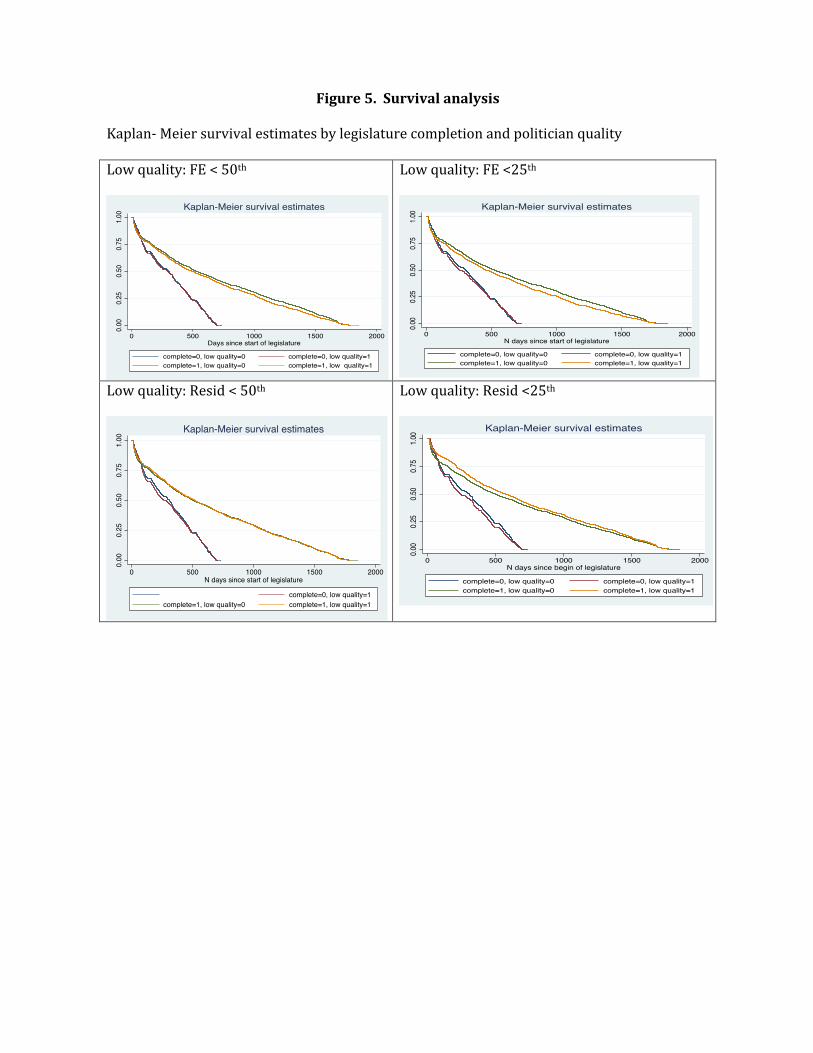
Figure  5.    Survival  analysis    Kaplan-­‐  Meier  survival  estimates  by  legislature  completion  and  politician  quality      Low  quality:  FE  <  50th      

 

Low  quality:  FE  <25th      

 Low  quality:  Resid  <  50th      

 

Low  quality:  Resid  <25th      

 

     

0.00

0.25

0.50

0.75

1.00

0 500 1000 1500 2000Days since start of legislature

complete=0, low quality=0 complete=0, low quality=1complete=1, low quality=0 complete=1, low quality=1

Kaplan-Meier survival estimates

0.00

0.25

0.50

0.75

1.00

0 500 1000 1500 2000N days since start of legislature

complete=0, low quality=0 complete=0, low quality=1complete=1, low quality=0 complete=1, low quality=1

Kaplan-Meier survival estimates

0.00

0.25

0.50

0.75

1.00

0 500 1000 1500 2000N days since start of legislature

complete=0, low quality=1complete=1, low quality=0 complete=1, low quality=1

Kaplan-Meier survival estimates0.0

00.2

50.5

00.7

51.0

0

0 500 1000 1500 2000N days since begin of legislature

complete=0, low quality=0 complete=0, low quality=1complete=1, low quality=0 complete=1, low quality=1

Kaplan-Meier survival estimates