From Mesh Generation to Scientific Visualization:An End-to-End Approach to Parallel Supercomputing

Tiankai Tu∗ Hongfeng Yu† Leonardo Ramirez-Guzman‡

Jacobo Bielak§ Omar Ghattas¶ Kwan-Liu Ma‖ David R. O’Hallaron∗∗

Abstract

Parallel supercomputing has traditionally focused on theinner kernel of scientific simulations: the solver. Thefront and back ends of the simulation pipeline—problemdescription and interpretation of the output—have taken aback seat to the solver when it comes to attention paidto scalability and performance, and are often relegated tooffline, sequential computation. As the largest simulationsmove beyond the realm of the terascale and into the petas-cale, this decomposition in tasks and platforms becomesincreasingly untenable. We propose an end-to-end approachin which all simulation components—meshing, partitioning,solver, and visualization—are tightly coupled and execute

∗Computer Science Department, Carnegie Mellon University,Pittsburgh, PA 15213, tutk@cs.cmu.edu

†Department of Computer Science, University of California,Davis, CA 95616, hfyu@ucdavis.edu

‡Department of Civil and Environmental Engineering,Carnegie Mellon University, Pittsburgh, PA 15213,lramirez@andrew.cmu.edu

§Department of Civil and Environmental Engineering, CarnegieMellon University, Pittsburgh, PA 15213, jbielak@andrew.cmu.edu

¶Institute for Computational Engineering and Sciences, JacksonSchool of Geosciences, and Departments of Mechanical Engineer-ing, Biomedical Engineering and Computer Sciences, The Univer-sity of Texas at Austin, Austin, TX 78077, omar@ices.utexas.edu

‖Department of Computer Science, University of California,Davis, CA 95616, ma@cs.ucdavis.edu

∗∗Computer Science Department and Department of Electricaland Computer Engineering, Carnegie Mellon University, PA15213, droh@cs.cmu.edu

Permission to make digital or hard copies of all or part ofthis work for personal or classroom use is granted without feeprovided that copies are not made or distributed for profit orcommercial advantage and that copies bear this notice and thefull citation on the first page. To copy otherwise, to republish, topost on servers or to redistribute to lists, requires prior specificpermission and/or a fee.

SC2006 November 2006, Tampa, Florida, USA0-7695-2700-0/06 $20.00 c©2006 IEEE

in parallel with shared data structures and no intermediateI/O. We present our implementation of this new approachin the context of octree-based finite element simulation ofearthquake ground motion. Performance evaluation on upto 2048 processors demonstrates the ability of the end-to-end approach to overcome the scalability bottlenecks of thetraditional approach.

1 Introduction

The traditional focus of parallel supercomputing has beenon the inner kernel of scientific simulations: the solver, aterm we use generically to refer to solution of (numericalapproximations of) the partial differential, ordinary differen-tial, algebraic, integral, or particle equations that govern thephysical system of interest. Great effort has gone into thedesign, evaluation, and performance optimization of scalableparallel solvers, and a number of Gordon Bell prizes haverecognized these achievements. However, the front andback ends of the simulation pipeline—problem descriptionand interpretation of the output—have taken a back seatto the solver when it comes to attention paid to scalabilityand performance. This of course makes sense: solvers areusually the most cycle-consuming component, which makesthem a natural target for performance optimization efforts forsuccessive generations of parallel architecture. The front andback ends, on the other hand, often have sufficiently smallmemory footprints and compute requirements that they canbe relegated to offline, sequential computation.

However, as scientific simulations move beyond therealm of the terascale and into the petascale, this decom-position in tasks and platforms becomes increasingly un-tenable. In particular, multiscale three-dimensional PDEsimulations often require variable-resolution unstructuredmeshes to efficiently resolve the spatially heterogeneousscales of behavior. The problem description phase canthen require generation of a massive unstructured mesh;the output interpretation phase then involves unstructured-mesh volume rendering of even larger size. As the largestunstructured mesh simulations move into the hundred mil-lion to billion element range, the memory and compute

requirements for mesh generation and volume renderingpreclude the use of sequential computers. On the other hand,scalable parallel algorithms and implementations for large-scale mesh generation and unstructured mesh volume visu-alization are significantly more difficult than their sequentialcounterparts.1

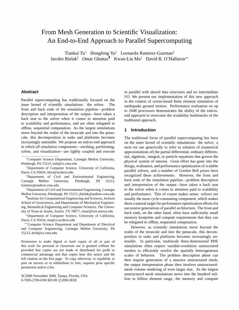
We have been working over the last several years todevelop methods to address some of these front-end andback-end performance bottlenecks, and have deployed themin support of large-scale simulations of earthquakes [3].For the front end, we have developed a computationaldatabase system that can be used to generate unstructuredhexahedral octree-based meshes with billions of elementson workstations with sufficiently large disks [26, 27, 28, 30].For the back end, we have developed special I/O strategiesthat effectively hide I/O costs when transferring individualtime step data to memory for rendering calculations [32],which themselves run in parallel and are highly scalable[16, 17, 19, 32]. Figure 1 illustrates the simulation pipelinein the context of our earthquake modeling problem, and,in particular, the sequence of files that are read and writtenbetween components.

Physical modeling

Meshing Partitioning Solving Visualizing

Scientific understanding

Vel

(m/s

)

time

FEM mesh~100GB

Partitioned mesh~1000 files

Spatial-temporal output ~10TB

Figure 1: Traditional simulation pipeline.

However, despite our best efforts at devising scalablealgorithms and implementations for the meshing, solver,and visualization components, as our resolution and fidelityrequirements have grown to target hundred million to multi-billion element simulations, significant bottlenecks remainin storing, transferring, and reading/writing multi-terabytefiles between these components. In particular, I/O of multi-terabyte files remains a pervasive performance bottleneck onparallel computers, to the extent that the offline approachto the meshing–partitioning–solver–visualization simulationpipeline becomes intractable for billion-unknown unstruc-tured mesh simulations. Ultimately, beyond scalability andI/O concerns, the biggest limitation of the offline approachis its inability to support interactive visualization of the

1For example, in a report identifying the prospects of scalabilityof a variety of parallel algorithms to petascale architectures [22],mesh generation and associated load balancing are categorized asClass 2, which includes algorithms that are expected to be “scalableprovided significant research challenges are overcome.”

simulation; the ability to debug and monitor the simulationat runtime based on volume-rendered visualizations becomesincreasingly crucial as problem size grows.

Thus, we are led to conclude that in order to (1)deliver necessary performance, scalability, and portabilityfor ultrascale unstructured mesh computations, (2) avoidunnecessary bottlenecks associated with multi-terabyte I/O,and (3) support runtime visualization steering, we must seekan end-to-end solution to the meshing–partitioning–solver–visualization parallel simulation pipeline. The key idea is toreplace the traditional, cumbersome file interface with a scal-able, parallel, runtime system that supports the simulationpipeline in two ways: (1) providing a common foundationon top of which all simulation components operate, and(2) serving as a medium for sharing data among simulationcomponents.

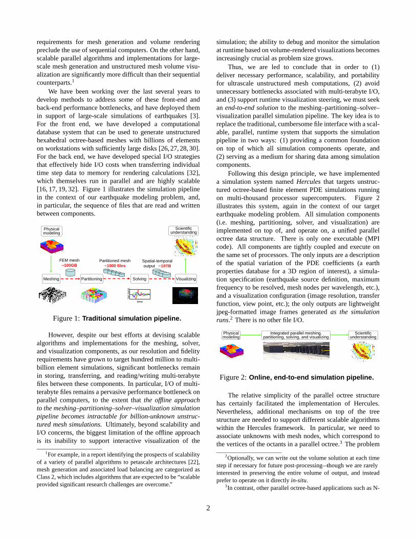
Following this design principle, we have implementeda simulation system named Hercules that targets unstruc-tured octree-based finite element PDE simulations runningon multi-thousand processor supercomputers. Figure 2illustrates this system, again in the context of our targetearthquake modeling problem. All simulation components(i.e. meshing, partitioning, solver, and visualization) areimplemented on top of, and operate on, a unified paralleloctree data structure. There is only one executable (MPIcode). All components are tightly coupled and execute onthe same set of processors. The only inputs are a descriptionof the spatial variation of the PDE coefficients (a earthproperties database for a 3D region of interest), a simula-tion specification (earthquake source definition, maximumfrequency to be resolved, mesh nodes per wavelength, etc.),and a visualization configuration (image resolution, transferfunction, view point, etc.); the only outputs are lightweightjpeg-formatted image frames generated as the simulationruns.2 There is no other file I/O.

Physical modeling

Scientific understanding

Integrated parallel meshing, partitioning, solving, and visualizing

Figure 2: Online, end-to-end simulation pipeline.

The relative simplicity of the parallel octree structurehas certainly facilitated the implementation of Hercules.Nevertheless, additional mechanisms on top of the treestructure are needed to support different scalable algorithmswithin the Hercules framework. In particular, we need toassociate unknowns with mesh nodes, which correspond tothe vertices of the octants in a parallel octree.3 The problem

2Optionally, we can write out the volume solution at each timestep if necessary for future post-processing—though we are rarelyinterested in preserving the entire volume of output, and insteadprefer to operate on it directly in-situ.

3In contrast, other parallel octree-based applications such as N-

2

of how to handle octree mesh nodes alone represents anontrivial challenge to meshing and solving. Furthermore,in order to provide unified data access services throughoutthe simulation pipeline, a flexible interface to the underlyingparallel octree has to be designed and exported such that allcomponents can share simulation data efficiently.

It is worth noting that while the only post-processingcomponent we have incorporated in Hercules is volumerendering visualization, there should be no technical dif-ficulty in adding other components. We have chosen 3Dvolume rendering over others mainly because it is one of themost demanding back ends in terms of algorithm complexityand difficulty of scalability. By demonstrating that online,integrated, highly parallel visualization is achievable, weestablish the viability of the proposed end-to-end approachand argue that it can be implemented for a wide variety ofother simulation pipeline configurations.

We have assessed the performance of Hercules on theAlpha EV68-based supercomputer at the Pittsburgh Super-computing Center for modeling earthquake ground motionin heterogeneous basins. Performance and scalability results(Section 4) show:

• Fixed-size scalability of the entire end-to-end simu-lation pipeline from 128 to 2048 processors at 64%overall parallel efficiency for 134 million mesh nodesimulations

• Isogranular scalability of the entire end-to-end simu-lation pipeline from 1 to 748 processors at combined81% parallel efficiency for 534 million mesh nodesimulations

• Isogranular scalability of the meshing, partitioning,and solver components at 60% parallel efficiency on2000 processors for 1.37 billion node simulations

We are able to demonstrate—we believe for the firsttime—scalability to 2048 processors of an entire end-to-endsimulation pipeline, from mesh generation to wave prop-agation to scientific visualization, using a unified, tightly-coupled, online, minimal I/O approach.

2 Octree-based finite element method

Octrees have been used as a basis for finite element approx-imation since at least the early 90s [31]. Our interest inoctrees stems from their ability to adapt to the wavelengthsof propagating seismic waves while maintaining a regularshape of finite elements. Here, leaves associated with thelowest level of the octree are identified with trilinear hexahe-dral finite elements and used for a Galerkin approximationof a suitable weak form of the elastic wave propagationequation. The hexahedra are recursively subdivided into8 elements until a local refinement criterion is satisfied.For seismic wave propagation in heterogeneous media, the

body simulations do not need to manipulate octants’ vertices.

criterion is that the longest element edge should be such thatthere result at least p nodes per wavelength, as determined bythe local shear wave velocity β and the maximum frequencyof interest fmax . In other words, hmax < β

pfmax. For trilinear

hexahedra and taking into account the accuracy with whichwe know typical basin properties, we usually take p = 10.An additional condition that drives mesh refinement is thatthe element size not differ by more than a factor of twoacross neighboring elements (the octree is then said to bebalanced). Note that the octree does not explicitly representmaterial interfaces within the earth, and instead accepts O(h)error in representing them implicitly. This is usually justifiedfor earthquake modeling since the location of interfaces isknown at best to the order of the seismic wavelength, i.e. toO(h). If warranted, higher-order accuracy in representingarbitrary interfaces can be achieved by local adjustment ofthe finite element basis (e.g., [31]).

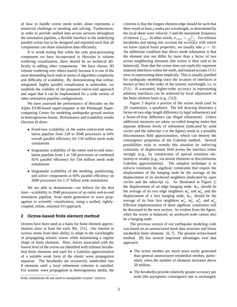
Figure 3 depicts a portion of the octree mesh (and its2D counterpart, a quadtree). The left drawing illustrates afactor-of-two edge length difference (a legal refinement) anda factor-of-four difference (an illegal refinement). Unlessadditional measures are taken, so-called hanging nodes thatseparate different levels of refinement (indicated by solidcircles and the subscript d in the figure) result in a possiblydiscontinuous field approximation, which can destroy theconvergence properties of the Galerkin method. Severalpossibilities exist to remedy this situation by enforcingcontinuity of displacement field across the interface eitherstrongly (e.g., by construction of special transition ele-ments) or weakly (e.g., via mortar elements or discontinuousGalerkin approximation). The simplest technique is toenforce continuity by algebraic constraints that require thedisplacement of the hanging node be the average of thedisplacement of its anchored neighbors (indicated by opencircles and the subscript a). As illustrated in Figure 3,the displacement of an edge hanging node, ud, should bethe average of its two edge neighbors ui

a and uja, and thedisplacement of a face hanging node, ud, should be theaverage of its four face neighbors ui

a, uja, uka, and ula.Efficient implementation of these algebraic constraints willbe discussed in the next section. As evident from the figure,when the octree is balanced, an anchored node cannot alsobe a hanging node.

The previous version of our earthquake modeling codewas based on an unstructured mesh data structure and lineartetrahedral finite elements [6, 7]. The present octree-basedmethod [8] has several important advantages over thatapproach:

• The octree meshes are much more easily generatedthan general unstructured tetrahedral meshes, partic-ularly when the number of elements increases above50 million.

• The hexahedra provide relatively greater accuracy pernode (the asymptotic convergence rate is unchanged,

3

d t dui

a ud uja

legal -

illegal¾

¡¡¡

¡¡¡

¡¡¡

¡¡¡

¡¡¡

¡¡¡

¡¡¡

¡¡¡

tt t

t

td d

d d

udud

uia uk

a

uja ul

a

t

d

hanging node

anchored node

Figure 3: Quadtree- and octree-based meshes.

but the constant is typically improved over tetrahedralapproximation).

• The hexahedra all have the same form of the elementstiffness matrices, scaled simply by element size andmaterial properties (which are stored as vectors), andthus no matrix storage is required at all. This resultsin a substantial decrease in required memory—aboutan order of magnitude, compared to our node-basedtetrahedral code.

• Because of the matrix-free implementation, (stiffness)matrix-vector products are carried out at the elementlevel. This produces much better cache utilization byrelegating the work that requires indirect addressing(and is memory bandwidth-limited) to vector opera-tions, and recasting the majority of the work of thematrix-vector product as local element-wise densematrix computations. The result is a significant boostin performance.

These features permit earthquake simulations to substan-tially higher frequencies and lower resolved shear wavevelocities than heretofore possible. In the next section, wedescribe the octree-based discretization and solution of theelastic wave equation.

2.1 Wave propagation model

We model seismic wave propagation in the earth via Navier’sequations of elastodynamics. Let u represent the vector fieldof the three displacement components; λ and µ the Lamemoduli and ρ the density distribution; b a time-dependentbody force representing the seismic source; t the surfacetraction vector; and Ω an open bounded domain in R

3 withfree surface ΓFS , truncation boundary ΓAB , and outwardunit normal to the boundary n. The initial–boundary value

problem is then written as:

ρ u − ∇ ·[µ(∇u + ∇u

T

)+ λ(∇ · u)I

]= b in Ω× (0, T ) ,

n × n × t = n × n × u√ρµ on ΓAB × (0, T ) ,

n · t = n · u√ρ(λ+ 2µ) on ΓAB × (0, T ) ,

(1)

t = 0 on ΓFS × (0, T ) ,

u = 0 in Ω× t = 0 ,

u = 0 in Ω× t = 0 ,

With this model, p waves propagate with velocity α =√(λ+ 2µ)/ρ, and s waves with velocity β =

√µ/ρ. The

continuous form above does not include material attenuation,which we introduce at the discrete level via a Rayleigh damp-ing model. The vector b comprises a set of body forces thatequilibrate an induced displacement dislocation on a faultplane, providing an effective representation of earthquakerupture on the plane. For example, for a seismic excitationidealized as a point source, b = −µvAMf(t)∇δ(x−ξ) [4].In this expression, v is the average earthquake dislocation;A the rupture area; M the (normalized) seismic momenttensor, which depends on the orientation of the fault; f(t) the(normalized) time evolution of the rupture; and ξ the sourcelocation.

Since we model earthquakes within a portion of theearth, we require appropriately positioned absorbing bound-aries to account for the truncated exterior. For simplicity, in(1) the absorbing boundaries are given as dashpots on ΓAB ,which approximate the tangential and normal componentsof the surface traction vector t with time derivatives ofcorresponding components of the displacement vector. Eventhough this absorbing boundary is a low-order approxima-tion of the true radiation condition, it is local in both spaceand time, which is particularly important for large-scaleparallel implementation. Finally, we enforce traction-freeconditions on the earth surface.

2.2 Octree discretization

We apply standard Galerkin finite element approximation inspace to the appropriate weak form of the initial-boundaryvalue problem (1). Let U be the space of admissible solutions(which depends on the regularity of b), Uh be a finite elementsubspace of U , and vh be a test function from that subspace.Then the weak form is written as follows:Find uh ∈ Uh such that∫

Ω

[ρuh · vh +

µ

2

(∇uh + ∇uT

h

)·(∇vh + ∇vT

h

)]dx

+

∫

Ω

[λ(∇ · uh)(∇ · vh)− b · vh] dx (2)

=

∫

ΓAB

√ρµ (n × n × uh) · (n × n × vh) ds

+

∫

ΓAB

√ρ(λ+ 2µ) (n · uh) (n · vh) ds, ∀vh ∈ Uh.

4

Finite element approximation is effected via piecewisetrilinear basis functions and associated trilinear hexahedralelements on an octree mesh. This strikes a balance betweensimplicity, low memory (since all element stiffness matricesare the same modulo scale factors), and reasonable accu-racy.4 Upon spatial discretization, we obtain a system ofordinary differential equations of the form

Mu +(C

AB + Catt

)u + Ku = b,

u(0) = 0, (3)

u(0) = 0,

where M and K are mass and stiffness matrices, arisingfrom the terms involving ρ and (µ, λ) in (2), respectively;b is a body force vector resulting from a discretization ofthe seismic source model; and damping matrix CAB reflectscontributions of the absorbing boundaries. We have alsointroduced the damping matrix Catt to simulate the effectof energy dissipation due to anelastic material behavior;it consists of a linear combination of mass and stiffnessmatrices and its form will be discussed in the next section.

2.3 Temporal approximation

The time dimension is discretized using central differences.The algorithm is made explicit using a diagonalization schemethat (1) lumps the mass matrix M , the absorbing boundarymatrix CAB , and the mass component of the the materialattenuation matrix Catt (all of which have Gram structureand are therefore spectrally equivalent to the identity), and(2) splits the diagonal and off-diagonal portions of thestiffness component of Catt, time-lagging the latter. Theresulting update for the displacement field at time step k+1is given by

[M +

∆t

2CAB

diag +∆t

2Catt

diag

]uk+1

=[2M −∆t2K − ∆t

2C

ABoff − ∆t

2C

attoff

]uk (4)

+[∆t

2C

AB +∆t

2C

att − M

]uk−1 +∆t2bk.

The time increment ∆t must satisfy a local CFL condi-tion for stability. Space is discretized over the octree mesh(each leaf corresponds to a hexahedral element) that resolveslocal seismic wavelengths as discussed above. This insuresthat the CFL-limited time step is of the order of that neededfor accuracy, and that excessive dispersion errors do not arisedue to over-refined meshes.

Spatial discretization via refinement of an octree pro-duces a non-conforming mesh, resulting in a discontinuousdisplacement approximation. We restore continuity of thedisplacement field across refinement interfaces by imposing

4The output quantities of greatest interest are displacements andvelocities, as opposed to stresses.

algebraic constraints that require the displacement at a hang-ing node to be consistent with the approximation along theneighboring element face or edge, as discussed above.

We can express these algebraic continuity constraints inthe form

u = Bu,

where u denotes the displacements at the anchored (i.e.,independent) nodes, and B is a sparse constraint matrix. Inparticular, Bij = 1

4if hanging node i is a face neighbor of

anchored node j and 1

2if it is an edge neighbor; Bij = 1

simply identifies a anchored node; and Bij = 0 otherwise.Rewriting the linear system (4) as

Auk+1 = c(uk,uk−1)

we can impose the continuity constraints via the projection

BTABuk+1 = B

Tc(uk,uk−1). (5)

The reduced matrix BTAB is then further lumped to renderit diagonal, so that the constrained update (5) is explicit. Infact the resulting reduced matrix can be constructed simplyby dividing the contributions of the hanging nodes andadding them in equal portions to diagonal components of thecorresponding anchored nodes. The righthand side of (5) isdetermined at each time step by computing c(uk,uk−1), i.e.the righthand side of (4), in an element-by-element fashion,and then applying the reduction BTc. This amounts againto dividing the contributions of the hanging components of cequally among the corresponding anchored nodes. The workinvolved in enforcing the constraints is proportional to thenumber of hanging nodes, which can be a sizable fraction ofthe overall number of nodes for a highly irregular octree, butis at most of O(N). Therefore, the per-iteration complexityof the update (5) remains linear in the number of nodes.

The combination of an octree-based wavelength-adaptivemesh, piecewise trilinear Galerkin finite elements in space,explicit central differences in time, constraints that enforcecontinuity of the displacement approximation, and local-in-space-and-time absorbing boundaries yields a second-order-accurate in time and space method that is capable of scalingup to the very large problem sizes that are required for highresolution earthquake modeling.

3 An end-to-end approach

The octree-based finite element method just described can beimplemented using a traditional, offline, file-based approach[3, 19, 26, 27, 32]. However, the inherent pitfalls, as outlinedin Section 1, cannot be eliminated unless we introduce amajor change in design principle.

Our new computational model thus follows the online,end-to-end approach overviewed in the Section 1. We viewdifferent components of a simulation pipeline as integralparts of a tightly-coupled parallel runtime system, ratherthan individual stand-alone programs. A number of technicaldifficulties emerge in the process of implementing this new

5

methodology within an octree-based finite element simu-lation system. This section discusses several fundamen-tal issues to be resolved, outlines the interfaces betweensimulation components, and presents a sketch of the corealgorithms.

Some of the techniques presented here are specific to thetarget class of octree-based methods. On the other hand, thedesign principles are more widely applicable; we hope theywill help accelerate the adoption of end-to-end approachesto parallel supercomputing where applicable.

3.1 Fundamental issues

Below we discuss fundamental issues encountered in de-veloping a scalable octree-based finite element simulationsystem. The solutions provided are critical to efficientimplementation of different simulation components.

3.1.1 Organizing a parallel octree

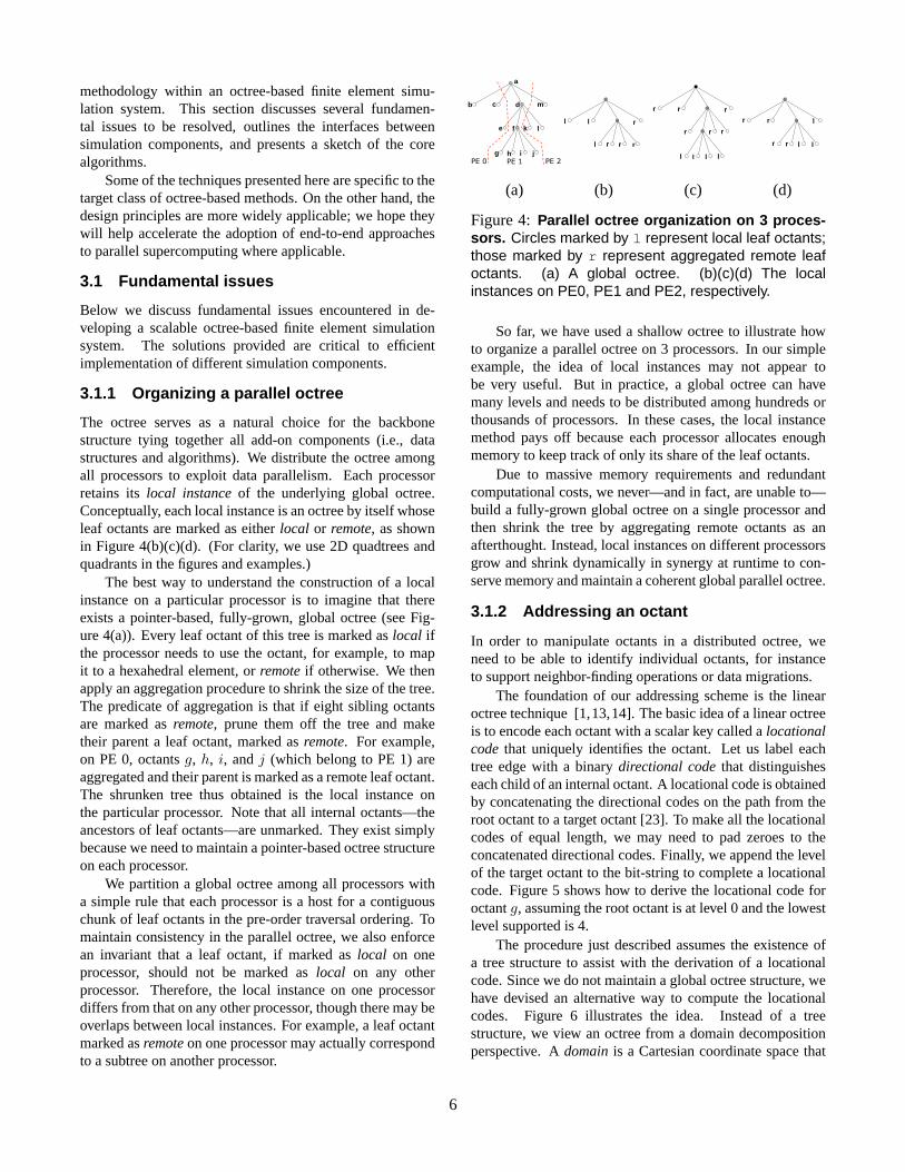
The octree serves as a natural choice for the backbonestructure tying together all add-on components (i.e., datastructures and algorithms). We distribute the octree amongall processors to exploit data parallelism. Each processorretains its local instance of the underlying global octree.Conceptually, each local instance is an octree by itself whoseleaf octants are marked as either local or remote, as shownin Figure 4(b)(c)(d). (For clarity, we use 2D quadtrees andquadrants in the figures and examples.)

The best way to understand the construction of a localinstance on a particular processor is to imagine that thereexists a pointer-based, fully-grown, global octree (see Fig-ure 4(a)). Every leaf octant of this tree is marked as local ifthe processor needs to use the octant, for example, to mapit to a hexahedral element, or remote if otherwise. We thenapply an aggregation procedure to shrink the size of the tree.The predicate of aggregation is that if eight sibling octantsare marked as remote, prune them off the tree and maketheir parent a leaf octant, marked as remote. For example,on PE 0, octants g, h, i, and j (which belong to PE 1) areaggregated and their parent is marked as a remote leaf octant.The shrunken tree thus obtained is the local instance onthe particular processor. Note that all internal octants—theancestors of leaf octants—are unmarked. They exist simplybecause we need to maintain a pointer-based octree structureon each processor.

We partition a global octree among all processors witha simple rule that each processor is a host for a contiguouschunk of leaf octants in the pre-order traversal ordering. Tomaintain consistency in the parallel octree, we also enforcean invariant that a leaf octant, if marked as local on oneprocessor, should not be marked as local on any otherprocessor. Therefore, the local instance on one processordiffers from that on any other processor, though there may beoverlaps between local instances. For example, a leaf octantmarked as remote on one processor may actually correspondto a subtree on another processor.

c d m

e f k l

g h ji

b

PE 0 PE 1 PE 2

a

r

l r

l r r

l

r r

r r r

l l ll

r

r

r l

r l l

r

(a) (b) (c) (d)

Figure 4: Parallel octree organization on 3 proces-sors. Circles marked by l represent local leaf octants;those marked by r represent aggregated remote leafoctants. (a) A global octree. (b)(c)(d) The localinstances on PE0, PE1 and PE2, respectively.

So far, we have used a shallow octree to illustrate howto organize a parallel octree on 3 processors. In our simpleexample, the idea of local instances may not appear tobe very useful. But in practice, a global octree can havemany levels and needs to be distributed among hundreds orthousands of processors. In these cases, the local instancemethod pays off because each processor allocates enoughmemory to keep track of only its share of the leaf octants.

Due to massive memory requirements and redundantcomputational costs, we never—and in fact, are unable to—build a fully-grown global octree on a single processor andthen shrink the tree by aggregating remote octants as anafterthought. Instead, local instances on different processorsgrow and shrink dynamically in synergy at runtime to con-serve memory and maintain a coherent global parallel octree.

3.1.2 Addressing an octant

In order to manipulate octants in a distributed octree, weneed to be able to identify individual octants, for instanceto support neighbor-finding operations or data migrations.

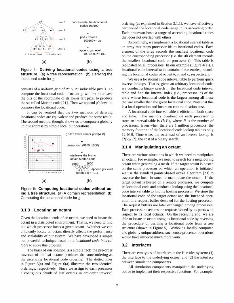
The foundation of our addressing scheme is the linearoctree technique [1,13,14]. The basic idea of a linear octreeis to encode each octant with a scalar key called a locationalcode that uniquely identifies the octant. Let us label eachtree edge with a binary directional code that distinguisheseach child of an internal octant. A locational code is obtainedby concatenating the directional codes on the path from theroot octant to a target octant [23]. To make all the locationalcodes of equal length, we may need to pad zeroes to theconcatenated directional codes. Finally, we append the levelof the target octant to the bit-string to complete a locationalcode. Figure 5 shows how to derive the locational code foroctant g, assuming the root octant is at level 0 and the lowestlevel supported is 4.

The procedure just described assumes the existence ofa tree structure to assist with the derivation of a locationalcode. Since we do not maintain a global octree structure, wehave devised an alternative way to compute the locationalcodes. Figure 6 illustrates the idea. Instead of a treestructure, we view an octree from a domain decompositionperspective. A domain is a Cartesian coordinate space that

6

a

c d m

e f k l

g h ji

b00 01 10 11

00 01 10 11

00 01 10 11

Level 0

Level 1

Level 2

Level 3

: Interior octant : Leaf octant

append g’s level 10010000

concatenate the directional codes 100100

pad 2 zeroes 100100 00

011

(a) (b)

Figure 5: Deriving locational codes using a treestructure. (a) A tree representation. (b) Deriving thelocational code for g.

consists of a uniform grid of 2n × 2n indivisible pixels. Tocompute the locational code of octant g, we first interleavethe bits of the coordinate of its lower left pixel to producethe so-called Morton code [21]. Then we append g’s level tocompose the locational code.

It can be verified that the two methods of derivinglocational codes are equivalent and produce the same result.The second method, though, allows us to compute a globallyunique address by simple local bit operations.

0 1 2 3 4 5 6 87 109 1211 13 14 15x

0

1

2

3

4

5

6

7

8

910

11

12

13

14

15

y

b c

eg h

i j

k l

m

0100

10010000

1000

interleave the bits to obtain Morton code

g’s left lower corner pixel(4, 8)

binary form (0100, 1000)

011append g’s level

(a) (b)

Figure 6: Computing locational codes without us-ing a tree structure. (a) A domain representation. (b)Computing the locational code for g.

3.1.3 Locating an octant

Given the locational code of an octant, we need to locate theoctant in a distributed environment. That is, we need to findout which processor hosts a given octant. Whether we canefficiently locate an octant directly affects the performanceand scalability of our system. We have developed a simplebut powerful technique based on a locational code intervaltable to solve this problem.

The basis of our solution is a simple fact: the pre-ordertraversal of the leaf octants produces the same ordering asthe ascending locational code ordering. The dotted linesin Figure 5(a) and Figure 6(a) illustrate the two identicalorderings, respectively. Since we assign to each processora contiguous chunk of leaf octants in pre-order traversal

ordering (as explained in Section 3.1.1), we have effectivelypartitioned the locational code range in its ascending order.Each processor hosts a range of ascending locational codesthat does not overlap with others.

Accordingly, we implement a locational interval table asan array that maps processor ids to locational codes. Eachelement of the array records the smallest locational codeon the corresponding processor (i.e. the ith element recordsthe smallest locational code on processor i). This table isreplicated on all processors. In our example (Figure 4(a)), alocational code interval table contains three entries, record-ing the locational codes of octant b, g, and k, respectively.

We use a locational code interval table to perform quickinverse lookups. That is, given an arbitrary locational code,we conduct a binary search in the locational code intervaltable and find the interval index (i.e., processor id) of theentry whose locational code is the largest among all thosethat are smaller than the given locational code. Note that thisis a local operation and incurs no communication cost.

A locational code interval table is efficient in both spaceand time. The memory overhead on each processor tostore an interval table is O(P ), where P is the number ofprocessors. Even when there are 1 million processors, thememory footprint of the locational code lookup table is only12 MB. Time-wise, the overhead of an inverse lookup isO(logP ), the cost of a binary search.

3.1.4 Manipulating an octant

There are various situations in which we need to manipulatean octant. For example, we need to search for a neighboringoctant when generating a mesh. If the target octant is hostedon the same processor on which an operation is initiated,we use the standard pointer-based octree algorithm [23] totraverse the local instance to manipulate the octant. If thetarget octant is hosted on a remote processor, we computeits locational code and conduct a lookup using the locationalcode interval table to find its hosting processor. We store thelocational code of the target octant and the intended oper-ation in a request buffer destined for the hosting processor.The request buffers are later exchanged among processors.Each processor executes the requests issued by its peers withrespect to its local octants. On the receiving end, we areable to locate an octant using its locational code by reversingthe procedure of deriving a locational code from a treestructure (shown in Figure 5). Without a locally computedand globally unique address, such cross-processor operationswould have involved much more work.

3.2 Interfaces

There are two types of interfaces in the Hercules system: (1)the interface to the underlying octree, and (2) the interfacebetween simulation components.

All simulation components manipulate the underlyingoctree to implement their respective functions. For example,

7

the mesher needs to refine or coarsen the tree structure toeffect necessary spatial discretization. The solver needsto attach runtime solution results to mesh nodes. Thevisualization component needs to process the attached data.In order to support such common operations efficiently, weimplement the backbone parallel octree in two abstract datatypes (ADTs): octant t and octree t, and provide asmall application program interface (API) to manipulate theADTs. For instance, at the octant level, we provide functionsto search for an octant, install an octant, and sprout or prunean octant. At the octree level, we support various tree traver-sal operations as well as the initialization and adjustment ofthe locational code lookup table. This interface allows usto encapsulate the complexity of manipulating the backboneparallel octrees within the abstract data types.

Note that there is one (and only one) exception to thecleanliness of the interface. We reserve a place-holderin octant t, that allows a simulation component (e.g.,a solver) to install a pointer to a data structure wherecomponent-specific data can be stored and retrieved. Nev-ertheless, such flexibility does not undermine the robustnessof the Hercules system because any structural changes tothe backbone octree must still be carried out through a pre-defined API call.

We have also designed binding interfaces between thesimulation components. However, unlike the octree/octantinterface, the inter-component interfaces can be clearly ex-plained only in the context of the simulation pipeline. There-fore, we defer the description of the inter-component in-terfaces to the next section where we outline the corealgorithms of individual simulation components.

3.3 Algorithms

Engineering a complex parallel simulation system like Her-cules not only involves careful software architectural design,but also demands non-trivial algorithmic innovations. Thissection highlights important algorithm and implementationfeatures of Hercules. We have omitted many of the technicaldetails.

3.3.1 Meshing and partitioning

We generate octree meshes online in-situ [29]. That is, wegenerate an octree mesh in parallel on the same processorswhere a solver and a visualizer will be running. Meshelements and nodes are created where they will be usedinstead of on remote processors. This strategy requiresthat mesh partitioning be an integral part of the meshingcomponent. The partitioning method we use is simple [5,11].We sort all octants in ascending locational code order, oftenreferred to as the Z-order [12], and divide them into equallength chunks in such a way that each processor will beassigned one and only one chunk. Because the locationalordering of the leaf octants corresponds exactly to the pre-order traversal of an octree, the partitioning and data redis-tribution often involve leaf octants migrating only between

adjacent processors. Whenever data migration occurs, localinstances of participating processors are adjusted to maintaina consistent global data structure. As shown in Section 4, thissimple strategy works well and yields almost ideal speedupfor fixed-size problems.

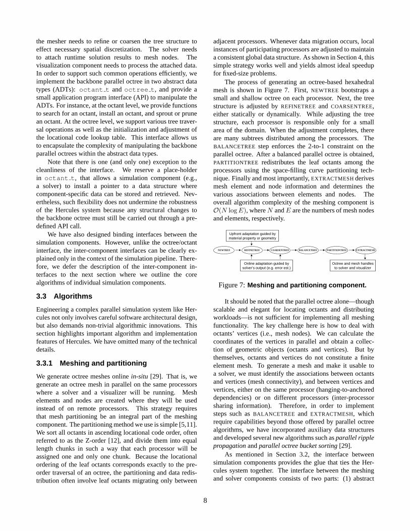
The process of generating an octree-based hexahedralmesh is shown in Figure 7. First, NEWTREE bootstraps asmall and shallow octree on each processor. Next, the treestructure is adjusted by REFINETREE and COARSENTREE,either statically or dynamically. While adjusting the treestructure, each processor is responsible only for a smallarea of the domain. When the adjustment completes, thereare many subtrees distributed among the processors. TheBALANCETREE step enforces the 2-to-1 constraint on theparallel octree. After a balanced parallel octree is obtained,PARTITIONTREE redistributes the leaf octants among theprocessors using the space-filling curve partitioning tech-nique. Finally and most importantly, EXTRACTMESH derivesmesh element and node information and determines thevarious associations between elements and nodes. Theoverall algorithm complexity of the meshing component isO(N logE), where N and E are the numbers of mesh nodesand elements, respectively.

NEWTREE REFINETREE COARSENTREE BALANCETREE PARTITIONTREE EXTRACTMESH

Octree and mesh handles to solver and visualizer

Upfront adaptation guided by material property or geometry

Online adaptation guided by solver’s output (e.g. error est.)

Figure 7: Meshing and partitioning component.

It should be noted that the parallel octree alone—thoughscalable and elegant for locating octants and distributingworkloads—is not sufficient for implementing all meshingfunctionality. The key challenge here is how to deal withoctants’ vertices (i.e., mesh nodes). We can calculate thecoordinates of the vertices in parallel and obtain a collec-tion of geometric objects (octants and vertices). But bythemselves, octants and vertices do not constitute a finiteelement mesh. To generate a mesh and make it usable toa solver, we must identify the associations between octantsand vertices (mesh connectivity), and between vertices andvertices, either on the same processor (hanging-to-anchoreddependencies) or on different processors (inter-processorsharing information). Therefore, in order to implementsteps such as BALANCETREE and EXTRACTMESH, whichrequire capabilities beyond those offered by parallel octreealgorithms, we have incorporated auxiliary data structuresand developed several new algorithms such as parallel ripplepropagation and parallel octree bucket sorting [29].

As mentioned in Section 3.2, the interface betweensimulation components provides the glue that ties the Her-cules system together. The interface between the meshingand solver components consists of two parts: (1) abstract

8

data types, and (2) callback functions. When meshing iscompleted, a mesh abstract data type (mesh t), along witha handle to the underlying octree (octree t), is passedforward to a solver. The mesh t ADT contains all theinformation a solver would need to initialize an executionenvironment. On the other hand, a solver controls thebehavior of a mesher via callback functions that are passedas parameters to the REFINETREE and COARSENTREE stepsat runtime. The latter interface allows us to perform runtimemesh adaptation, which is critical for future extension of theHercules framework to support solution adaptivity.

3.3.2 Solver

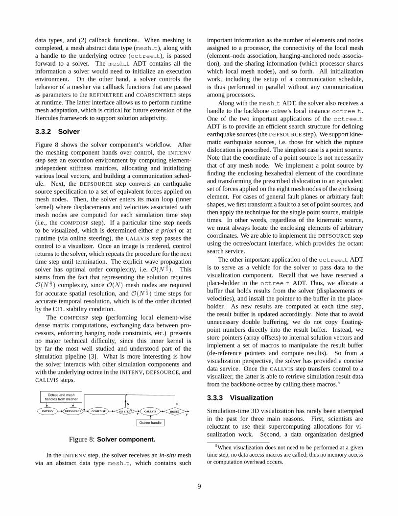
Figure 8 shows the solver component’s workflow. Afterthe meshing component hands over control, the INITENV

step sets an execution environment by computing element-independent stiffness matrices, allocating and initializingvarious local vectors, and building a communication sched-ule. Next, the DEFSOURCE step converts an earthquakesource specification to a set of equivalent forces applied onmesh nodes. Then, the solver enters its main loop (innerkernel) where displacements and velocities associated withmesh nodes are computed for each simulation time step(i.e., the COMPDISP step). If a particular time step needsto be visualized, which is determined either a priori or atruntime (via online steering), the CALLVIS step passes thecontrol to a visualizer. Once an image is rendered, controlreturns to the solver, which repeats the procedure for the nexttime step until termination. The explicit wave propagationsolver has optimal order complexity, i.e. O(N

4

3 ). Thisstems from the fact that representing the solution requiresO(N

4

3 ) complexity, since O(N) mesh nodes are requiredfor accurate spatial resolution, and O(N

1

3 ) time steps foraccurate temporal resolution, which is of the order dictatedby the CFL stability condition.

The COMPDISP step (performing local element-wisedense matrix computations, exchanging data between pro-cessors, enforcing hanging node constraints, etc.) presentsno major technical difficulty, since this inner kernel isby far the most well studied and understood part of thesimulation pipeline [3]. What is more interesting is howthe solver interacts with other simulation components andwith the underlying octree in the INITENV, DEFSOURCE, andCALLVIS steps.

INITENV DEFSOURCE COMPDISP

Octree and mesh handles from mesher

VIS STEP? CALLVIS DONE?

Octree handle

N N

Y Y

Figure 8: Solver component.

In the INITENV step, the solver receives an in-situ meshvia an abstract data type mesh t, which contains such

important information as the number of elements and nodesassigned to a processor, the connectivity of the local mesh(element–node association, hanging-anchored node associa-tion), and the sharing information (which processor shareswhich local mesh nodes), and so forth. All initializationwork, including the setup of a communication schedule,is thus performed in parallel without any communicationamong processors.

Along with the mesh t ADT, the solver also receives ahandle to the backbone octree’s local instance octree t.One of the two important applications of the octree tADT is to provide an efficient search structure for definingearthquake sources (the DEFSOURCE step). We support kine-matic earthquake sources, i.e. those for which the rupturedislocation is prescribed. The simplest case is a point source.Note that the coordinate of a point source is not necessarilythat of any mesh node. We implement a point source byfinding the enclosing hexahedral element of the coordinateand transforming the prescribed dislocation to an equivalentset of forces applied on the eight mesh nodes of the enclosingelement. For cases of general fault planes or arbitrary faultshapes, we first transform a fault to a set of point sources, andthen apply the technique for the single point source, multipletimes. In other words, regardless of the kinematic source,we must always locate the enclosing elements of arbitrarycoordinates. We are able to implement the DEFSOURCE stepusing the octree/octant interface, which provides the octantsearch service.

The other important application of the octree t ADTis to serve as a vehicle for the solver to pass data to thevisualization component. Recall that we have reserved aplace-holder in the octree t ADT. Thus, we allocate abuffer that holds results from the solver (displacements orvelocities), and install the pointer to the buffer in the place-holder. As new results are computed at each time step,the result buffer is updated accordingly. Note that to avoidunnecessary double buffering, we do not copy floating-point numbers directly into the result buffer. Instead, westore pointers (array offsets) to internal solution vectors andimplement a set of macros to manipulate the result buffer(de-reference pointers and compute results). So from avisualization perspective, the solver has provided a concisedata service. Once the CALLVIS step transfers control to avisualizer, the latter is able to retrieve simulation result datafrom the backbone octree by calling these macros.5

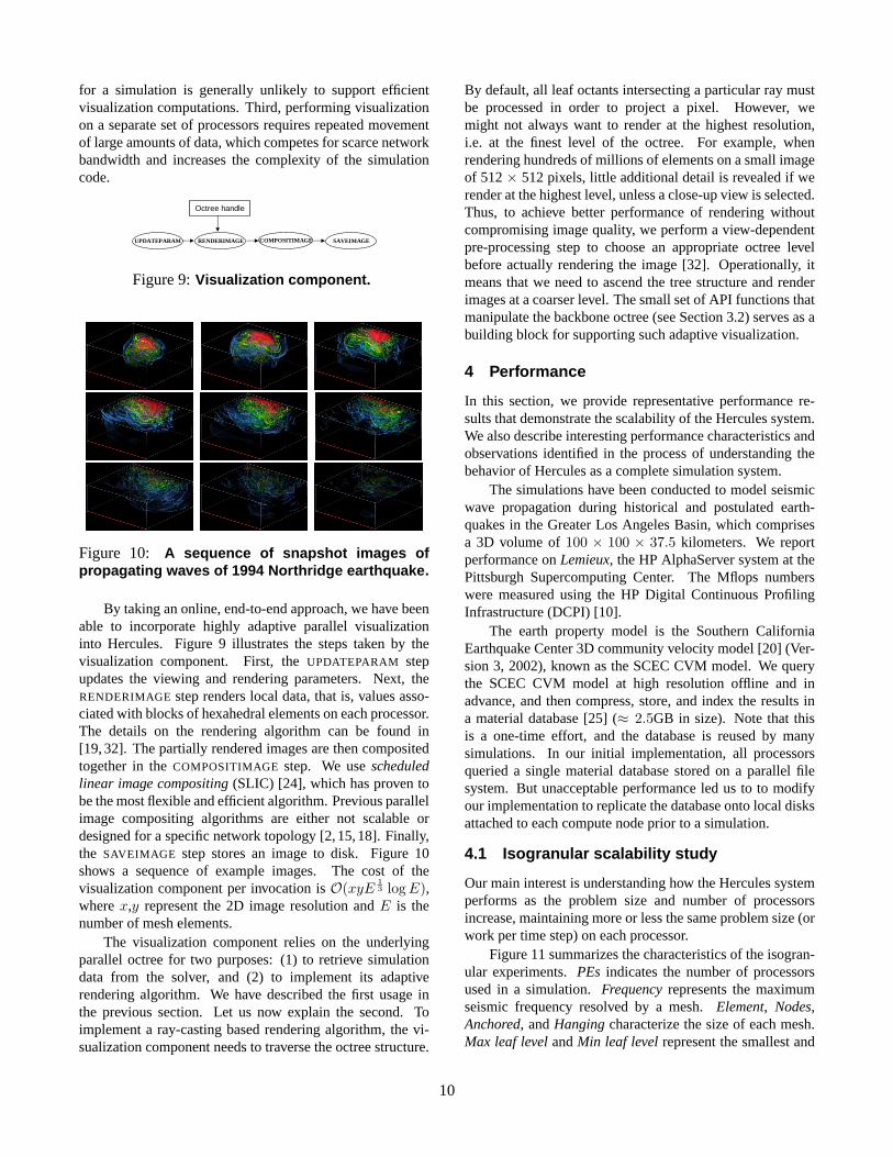
3.3.3 Visualization

Simulation-time 3D visualization has rarely been attemptedin the past for three main reasons. First, scientists arereluctant to use their supercomputing allocations for vi-sualization work. Second, a data organization designed

5When visualization does not need to be performed at a giventime step, no data access macros are called; thus no memory accessor computation overhead occurs.

9

for a simulation is generally unlikely to support efficientvisualization computations. Third, performing visualizationon a separate set of processors requires repeated movementof large amounts of data, which competes for scarce networkbandwidth and increases the complexity of the simulationcode.

UPDATEPARAM

Octree handle

RENDERIMAGE COMPOSITIMAGE SAVEIMAGE

Figure 9: Visualization component.

Figure 10: A sequence of snapshot images ofpropagating waves of 1994 Northridge earthquake.

By taking an online, end-to-end approach, we have beenable to incorporate highly adaptive parallel visualizationinto Hercules. Figure 9 illustrates the steps taken by thevisualization component. First, the UPDATEPARAM stepupdates the viewing and rendering parameters. Next, theRENDERIMAGE step renders local data, that is, values asso-ciated with blocks of hexahedral elements on each processor.The details on the rendering algorithm can be found in[19, 32]. The partially rendered images are then compositedtogether in the COMPOSITIMAGE step. We use scheduledlinear image compositing (SLIC) [24], which has proven tobe the most flexible and efficient algorithm. Previous parallelimage compositing algorithms are either not scalable ordesigned for a specific network topology [2, 15, 18]. Finally,the SAVEIMAGE step stores an image to disk. Figure 10shows a sequence of example images. The cost of thevisualization component per invocation is O(xyE

1

3 logE),where x,y represent the 2D image resolution and E is thenumber of mesh elements.

The visualization component relies on the underlyingparallel octree for two purposes: (1) to retrieve simulationdata from the solver, and (2) to implement its adaptiverendering algorithm. We have described the first usage inthe previous section. Let us now explain the second. Toimplement a ray-casting based rendering algorithm, the vi-sualization component needs to traverse the octree structure.

By default, all leaf octants intersecting a particular ray mustbe processed in order to project a pixel. However, wemight not always want to render at the highest resolution,i.e. at the finest level of the octree. For example, whenrendering hundreds of millions of elements on a small imageof 512 × 512 pixels, little additional detail is revealed if werender at the highest level, unless a close-up view is selected.Thus, to achieve better performance of rendering withoutcompromising image quality, we perform a view-dependentpre-processing step to choose an appropriate octree levelbefore actually rendering the image [32]. Operationally, itmeans that we need to ascend the tree structure and renderimages at a coarser level. The small set of API functions thatmanipulate the backbone octree (see Section 3.2) serves as abuilding block for supporting such adaptive visualization.

4 Performance

In this section, we provide representative performance re-sults that demonstrate the scalability of the Hercules system.We also describe interesting performance characteristics andobservations identified in the process of understanding thebehavior of Hercules as a complete simulation system.

The simulations have been conducted to model seismicwave propagation during historical and postulated earth-quakes in the Greater Los Angeles Basin, which comprisesa 3D volume of 100 × 100 × 37.5 kilometers. We reportperformance on Lemieux, the HP AlphaServer system at thePittsburgh Supercomputing Center. The Mflops numberswere measured using the HP Digital Continuous ProfilingInfrastructure (DCPI) [10].

The earth property model is the Southern CaliforniaEarthquake Center 3D community velocity model [20] (Ver-sion 3, 2002), known as the SCEC CVM model. We querythe SCEC CVM model at high resolution offline and inadvance, and then compress, store, and index the results ina material database [25] (≈ 2.5GB in size). Note that thisis a one-time effort, and the database is reused by manysimulations. In our initial implementation, all processorsqueried a single material database stored on a parallel filesystem. But unacceptable performance led us to to modifyour implementation to replicate the database onto local disksattached to each compute node prior to a simulation.

4.1 Isogranular scalability study

Our main interest is understanding how the Hercules systemperforms as the problem size and number of processorsincrease, maintaining more or less the same problem size (orwork per time step) on each processor.

Figure 11 summarizes the characteristics of the isogran-ular experiments. PEs indicates the number of processorsused in a simulation. Frequency represents the maximumseismic frequency resolved by a mesh. Element, Nodes,Anchored, and Hanging characterize the size of each mesh.Max leaf level and Min leaf level represent the smallest and

10

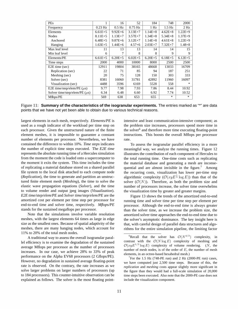
PEs 1 16 52 184 748 2000Frequency 0.23 Hz 0.5 Hz 0.75 Hz 1 Hz 1.5 Hz 2 HzElements 6.61E+5 9.92E+6 3.13E+7 1.14E+8 4.62E+8 1.22E+9Nodes 8.11E+5 1.13E+7 3.57E+7 1.34E+8 5.34E+8 1.37E+9

Anchored 6.48E+5 9.87E+6 3.12E+7 1.14E+8 4.61E+8 1.22E+9Hanging 1.63E+5 1.44E+6 4.57+6 2.03E+7 7.32E+7 1.48+8

Max leaf level 11 13 13 14 14 15Min leaf level 6 7 8 8 9 9Elements/PE 6.61E+5 6.20E+5 6.02E+5 6.20E+5 6.18E+5 6.12E+5Time steps 2000 4000 10000 8000 2500 2500E2E time (sec) 12911 19804 38165 48668 13033 16709

Replication (sec) 22 71 85 94 187 251Meshing (sec) 20 75 128 150 303 333Solver (sec) 8381 16060 31781 42892 11960 16097Visualization (sec) 4488 3596 6169 5528 558 *

E2E time/step/elem/PE (µs) 9.77 7.98 7.93 7.86 8.44 10.92Solver time/step/elem/PE (µs) 6.34 6.48 6.60 6.92 7.74 10.52Mflops/PE 569 638 653 655 * *

Figure 11: Summary of the characteristics of the isogranular experiments. The entries marked as “*” are datapoints that we have not yet been able to obtain due to various technical reasons.

largest elements in each mesh, respectively. Elements/PE isused as a rough indicator of the workload per time step oneach processor. Given the unstructured nature of the finiteelement meshes, it is impossible to guarantee a constantnumber of elements per processor. Nevertheless, we havecontained the difference to within 10%. Time steps indicatesthe number of explicit time steps executed. The E2E timerepresents the absolute running time of a Hercules simulationfrom the moment the code is loaded onto a supercomputer tothe moment it exits the system. This time includes the timeof replicating a material database stored on a shared parallelfile system to the local disk attached to each compute node(Replication), the time to generate and partition an unstruc-tured finite element mesh (Meshing), the time to solve theelastic wave propagation equations (Solver), and the timeto volume render and output jpeg images (Visualization).E2E time/step/elem/PE and Solver time/step/elem/PE are theamortized cost per element per time step per processor forend-to-end time and solver time, respectively. Mflops/PEstands for the sustained megaflops per processor.

Note that the simulations involve variable resolutionmeshes, with the largest elements 64 times as large in edgesize as the smallest ones. Because of spatial adaptivity of themeshes, there are many hanging nodes, which account for11% to 20% of the total mesh nodes.

A traditional way to assess the overall isogranular paral-lel efficiency is to examine the degradation of the sustainedaverage Mflops per processor as the number of processorsincreases. In our case, we achieve 28% to 33% of peakperformance on the Alpha EV68 processors (2 Gflops/PE).However, no degradation in sustained average floating-pointrate is observed. On the contrary, the rate increases as wesolve larger problems on larger numbers of processors (upto 184 processors). This counter-intuitive observation can beexplained as follows. The solver is the most floating point-

intensive and least communication-intensive component; asthe problem size increases, processors spend more time inthe solver6 and therefore more time executing floating-pointinstructions. This boosts the overall Mflops per processorrate.

To assess the isogranular parallel efficiency in a moremeaningful way, we analyze the running times. Figure 12illustrates the contribution of each component of Hercules tothe total running time. One-time costs such as replicatingthe material database and generating a mesh are inconse-quential and are almost invisible in the figure.7 Amongthe recurring costs, visualization has lower per-time stepalgorithmic complexity (O(xyE

1

3 logE)) than that of thesolver (O(N)). Therefore, as both the problem size andnumber of processors increase, the solver time overwhelmsthe visualization time by greater and greater margins.

Figure 13 shows the trends of the amortized end-to-endrunning time and solver time per time step per element perprocessor. Although the end-to-end time is always greaterthan the solver time, as we increase the problem size, theamortized solver time approaches the end-to-end time due tothe solver’s asymptotic dominance. The key insight here isthat, with careful design of parallel data structures and algo-rithms for the entire simulation pipeline, the limiting factor

6Recall that the solver has O(N4/3) complexity, incontrast with the O(N logE) complexity of meshing andO(xyE1/3 logE) complexity of volume rendering. (N , thenumber of mesh nodes, is of the order of E, the number of meshelements, in an octree-based hexahedral mesh.)

7For the 1.5 Hz (748-PE run) and 2 Hz (2000-PE run) cases,we have computed just 2,500 time steps. Because of this, thereplication and meshing costs appear slightly more significant inthe figure than they would had a full-scale simulation of 20,000time steps been executed. Also note that the 2000-PE case does notinclude the visualization component.

11

0%

20%

40%

60%

80%

100%

1PE 16PE 52PE 184PE 748PE 2000PE

Replicating Meshing Solving Visualizing

Figure 12: The percentage contribution of eachsimulation component to the total running time.

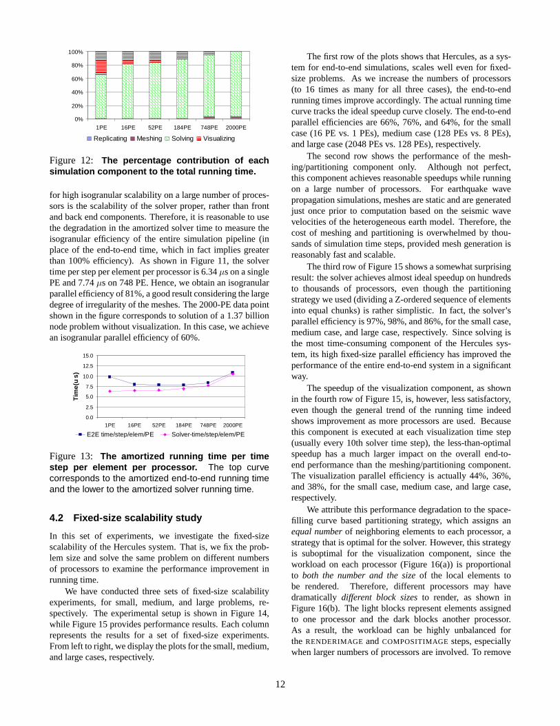
for high isogranular scalability on a large number of proces-sors is the scalability of the solver proper, rather than frontand back end components. Therefore, it is reasonable to usethe degradation in the amortized solver time to measure theisogranular efficiency of the entire simulation pipeline (inplace of the end-to-end time, which in fact implies greaterthan 100% efficiency). As shown in Figure 11, the solvertime per step per element per processor is 6.34 µs on a singlePE and 7.74 µs on 748 PE. Hence, we obtain an isogranularparallel efficiency of 81%, a good result considering the largedegree of irregularity of the meshes. The 2000-PE data pointshown in the figure corresponds to solution of a 1.37 billionnode problem without visualization. In this case, we achievean isogranular parallel efficiency of 60%.

0.0

2.5

5.0

7.5

10.0

12.5

15.0

1PE 16PE 52PE 184PE 748PE 2000PE

Tim

e(u

s)

E2E time/step/elem/PE Solver-time/step/elem/PE

Figure 13: The amortized running time per timestep per element per processor. The top curvecorresponds to the amortized end-to-end running timeand the lower to the amortized solver running time.

4.2 Fixed-size scalability study

In this set of experiments, we investigate the fixed-sizescalability of the Hercules system. That is, we fix the prob-lem size and solve the same problem on different numbersof processors to examine the performance improvement inrunning time.

We have conducted three sets of fixed-size scalabilityexperiments, for small, medium, and large problems, re-spectively. The experimental setup is shown in Figure 14,while Figure 15 provides performance results. Each columnrepresents the results for a set of fixed-size experiments.From left to right, we display the plots for the small, medium,and large cases, respectively.

The first row of the plots shows that Hercules, as a sys-tem for end-to-end simulations, scales well even for fixed-size problems. As we increase the numbers of processors(to 16 times as many for all three cases), the end-to-endrunning times improve accordingly. The actual running timecurve tracks the ideal speedup curve closely. The end-to-endparallel efficiencies are 66%, 76%, and 64%, for the smallcase (16 PE vs. 1 PEs), medium case (128 PEs vs. 8 PEs),and large case (2048 PEs vs. 128 PEs), respectively.

The second row shows the performance of the mesh-ing/partitioning component only. Although not perfect,this component achieves reasonable speedups while runningon a large number of processors. For earthquake wavepropagation simulations, meshes are static and are generatedjust once prior to computation based on the seismic wavevelocities of the heterogeneous earth model. Therefore, thecost of meshing and partitioning is overwhelmed by thou-sands of simulation time steps, provided mesh generation isreasonably fast and scalable.

The third row of Figure 15 shows a somewhat surprisingresult: the solver achieves almost ideal speedup on hundredsto thousands of processors, even though the partitioningstrategy we used (dividing a Z-ordered sequence of elementsinto equal chunks) is rather simplistic. In fact, the solver’sparallel efficiency is 97%, 98%, and 86%, for the small case,medium case, and large case, respectively. Since solving isthe most time-consuming component of the Hercules sys-tem, its high fixed-size parallel efficiency has improved theperformance of the entire end-to-end system in a significantway.

The speedup of the visualization component, as shownin the fourth row of Figure 15, is, however, less satisfactory,even though the general trend of the running time indeedshows improvement as more processors are used. Becausethis component is executed at each visualization time step(usually every 10th solver time step), the less-than-optimalspeedup has a much larger impact on the overall end-to-end performance than the meshing/partitioning component.The visualization parallel efficiency is actually 44%, 36%,and 38%, for the small case, medium case, and large case,respectively.

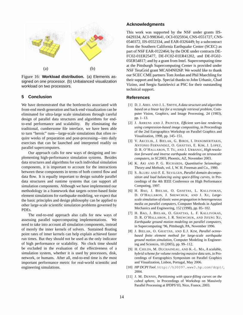
We attribute this performance degradation to the space-filling curve based partitioning strategy, which assigns anequal number of neighboring elements to each processor, astrategy that is optimal for the solver. However, this strategyis suboptimal for the visualization component, since theworkload on each processor (Figure 16(a)) is proportionalto both the number and the size of the local elements tobe rendered. Therefore, different processors may havedramatically different block sizes to render, as shown inFigure 16(b). The light blocks represent elements assignedto one processor and the dark blocks another processor.As a result, the workload can be highly unbalanced forthe RENDERIMAGE and COMPOSITIMAGE steps, especiallywhen larger numbers of processors are involved. To remove

12

PEs 1 2 4 8 16 32 64 128 256 512 1024 2048

Small case (0.23 Hz, 0.8M nodes) x x x x xMedium case (0.5 Hz, 11M nodes) x x x x xLarge case (1 Hz, 134M nodes) x x x x x

Figure 14: Setup of fixed-size speedup experiments. Entries marked with “x” represent experiment runs.

0

2000

4000

6000

8000

10000

12000

14000

0 4 8 12 16

E2E time Ideal speedup time

0

5000

1000015000

20000

2500030000

3500040000

0 16 32 48 64 80 96 112 128

E2E time Ideal speedup time

02000400060008000

1000012000140001600018000

0 256 512 768 1024 1280 1536 1792 2048

E2E time Ideal speedup time

Small case end-to-end time Medium case end-to-end time Large case end-to-end time

02468

10121416182022

0 4 8 12 16

Meshing time Ideal speedup time

0102030405060708090

100110

0 16 32 48 64 80 96 112 128

Meshing time Ideal speedup time

0255075

100125150175200225

0 256 512 768 1024 1280 1536 1792 2048

Meshing time Ideal speedup time

Small case meshing time Medium case meshing time Large case meshing time

0100020003000400050006000700080009000

0 4 8 12 16

Sovling time Ideal speedup time

0

5000

10000

15000

20000

25000

30000

35000

0 16 32 48 64 80 96 112 128

Solving time Ideal speedup time

0

2000

40006000

8000

1000012000

1400016000

0 256 512 768 1024 1280 1536 1792 2048

Solving time Ideal speedup time

Small case solver time Medium case solver time Large case solver time

0500

100015002000250030003500400045005000

0 4 8 12 16

Visualizing time Ideal speedup time

0

1000

2000

3000

4000

5000

6000

7000

0 16 32 48 64 80 96 112 128

Visualzing time Ideal speeup time

0200

400600

8001000

12001400

1600

0 256 512 768 1024 1280 1536 1792 2048

Visualizing time Ideal speedup time

Small case visualization time Medium case visualization time Large case visualization time

Figure 15: Speedups of fixed-size experiments. The horizontal axes represent the number of processors. Thevertical axes represent the running time in seconds. The first row shows the end-to-end running time; the secondthe meshing and partitioning time; the third the solver time; and the fourth the visualization time.

this performance bottleneck, a viable approach is to use anew hybrid rendering scheme that balances the workloaddynamically by taking into account the cost of transferringelements versus that of pixels [9]. An element is renderedlocally only if the rendering cost is lower than the costof sending the resulting projected image to the processor

responsible for compositing the image. Alternatively, we canre-evaluate the space-filling curve based partitioning strategyand develop a new scheme that better accommodates both thesolver and the visualization components. Striking a balancebetween the data distributions for the two is an inherent issuefor parallel end-to-end simulations.

13

(a) (b)

Figure 16: Workload distribution. (a) Elements as-signed on one processor. (b) Unbalanced visualizationworkload on two processors.

5 Conclusion

We have demonstrated that the bottlenecks associated withfront-end mesh generation and back-end visualization can beeliminated for ultra-large scale simulations through carefuldesign of parallel data structures and algorithms for end-to-end performance and scalability. By eliminating thetraditional, cumbersome file interface, we have been ableto turn “heroic” runs—large-scale simulations that often re-quire weeks of preparation and post-processing—into dailyexercises that can be launched and interpreted readily onparallel supercomputers.

Our approach calls for new ways of designing and im-plementing high-performance simulation systems. Besidesdata structures and algorithms for each individual simulationcomponents, it is important to account for the interactionsbetween these components in terms of both control flow anddata flow. It is equally important to design suitable paralleldata structures and runtime systems that can support allsimulation components. Although we have implemented ourmethodology in a framework that targets octree-based finiteelement simulations for earthquake modeling, we expect thatthe basic principles and design philosophy can be applied toother large-scale scientific simulation problems governed byPDEs.

The end-to-end approach also calls for new ways ofassessing parallel supercomputing implementations. Weneed to take into account all simulation components, insteadof merely the inner kernels of solvers. Sustained floatingpoint rates of inner kernels can help explain achieved fasterrun times. But they should not be used as the only indicatorof high performance or scalability. No clock time shouldbe excluded in the evaluation of the effectiveness of asimulation system, whether it is used by processors, disk,network, or humans. After all, end-to-end time is the mostimportant performance metric for real-world scientific andengineering simulations.

Acknowledgments

This work was supported by the NSF under grants IIS-0429334, ACI-9983641, OCI-0325934, CNS-0551727, CNS-0540372, IIS-0552334, and EAR-0326449; by a subcontractfrom the Southern California Earthquake Center (SCEC) aspart of NSF EAR-0122464; by the DOE under contracts DE-FC02-01ER25477, DE-FC02-01ER41202, and DE-FG02-05ER54817; and by a grant from Intel. Supercomputing timeat the Pittsburgh Supercomputing Center is provided underNSF TeraGrid grant MCA04N026P. We would like to thankour SCEC CME partners Tom Jordan and Phil Maechling fortheir support and help. Special thanks to John Urbanic, ChadVizino, and Sergiu Sanielevici at PSC for their outstandingtechnical support.

References

[1] D. J. ABEL AND J. L. SMITH, A data structure and algorithmbased on a linear key for a rectangle retrieval problem, Com-puter Vision, Graphics, and Image Processing, 24 (1983),pp. 1–13.

[2] J. AHRENS AND J. PAINTER, Efficient sort-last renderingusing compression-based image compositing, in Proceedingsof the 2nd Eurographics Workshop on Parallel Graphics andVisualization, 1998, pp. 145–151.

[3] V. AKCELIK, J. BIELAK, G. BIROS, I. IPANOMERITAKIS,ANTONIO FERNANDEZ, O. GHATTAS, E. KIM, J. LOPEZ,D. R. O’HALLARON, T. TU, AND J. URBANIC, High resolu-tion forward and inverse earthquake modeling on terasacalecomputers, in SC2003, Phoenix, AZ, November 2003.

[4] K. AKI AND P. G. RICHARDS, Quantitative Seismology:Theory and Methods, vol. I, W. H. Freeman and Co., 1980.

[5] S. ALURU AND F. E. SEVILGEN, Parallel domain decompo-sition and load balancing using space-filling curves, in Pro-ceedings of the 4th IEEE Conference on High PerformanceComputing, 1997.

[6] H. BAO, J. BIELAK, O. GHATTAS, L. KALLIVOKAS,D. O’HALLARON, J. SHEWCHUK, AND J. XU, Large-scale simulation of elastic wave propagation in heterogeneousmedia on parallel computers, Computer Methods in AppliedMechanics and Engineering, 152 (1998), pp. 85–102.

[7] H. BAO, J. BIELAK, O. GHATTAS, L. F. KALLIVOKAS,D. R. O’HALLARON, J. R. SHEWCHUK, AND JIFENG XU,Earthquake ground motion modeling on parallel computers,in Supercomputing ’96, Pittsburgh, PA, November 1996.

[8] J. BIELAK, O. GHATTAS, AND E.J. KIM, Parallel octree-based finite element method for large-scale earthquakeground motion simulation, Computer Modeling in Engineer-ing and Sciences, 10 (2005), pp. 99–112.

[9] H. CHILDS, M. DUCHAINEAU, AND K.-L. MA, A scalable,hybrid scheme for volume rendering massive data sets, in Pro-ceedings of Eurographics Symposium on Parallel Graphicsand Visualization, Lisbon, Portugal, May 2006.

[10] HP DCPI Tool. http://h30097.www3.hp.com/dcpi/,2004.

[11] J. M. DENNIS, Partitioning with space-filling curves on thecubed sphere, in Proceedings of Workshop on MassivelyParallel Processing at IPDPS’03, Nice, France, 2003.

14

[12] C. FALOUTSOS AND S. ROSEMAN, Fractals for secondarykey retrieval, in Proceedings of the Eighth ACM SIGACT-SIGMID-SIGART Symposium on Principles of DatabaseSystems (PODS), 1989.

[13] I. GARGANTINI, An effective way to represent quadtrees,Communications of the ACM, 25 (1982), pp. 905–910.

[14] , Linear octree for fast processing of three-dimensionalobjects, Computer Graphics and Image Processing, 20 (1982),pp. 365–374.

[15] T.-Y. LEE, C. S. RAGHAVENDRA, AND J. B. NICHOLAS,Image composition schemes for sort-last polygon renderingon 2D mesh multicomputers, IEEE Transactions on Visual-ization and Computer Graphics, 2 (1996), pp. 202–217.

[16] K.-L. MA AND T. CROCKETT, A scalable parallel cell-projection volume rendering algorithm for three-dimensionalunstructured data, in Proceedings of 1997 Symposium onParallel Rendering, 1997, pp. 95–104.

[17] , Parallel visualization of large-scale aerodynamicscalculations: A case study on the Cray T3E, in Proceedings of1999 IEEE Parallel Visualization and Graphics Symposium,San Francisco, CA, October 1999, pp. 15–20.

[18] K.-L. MA, J. S. PAINTER, C. D. HANSEN, AND M. F.KROGH, Parallel volume rendering using binary-swap com-positing, IEEE Computer Graphics and Applications, 14(1994), pp. 59–67.

[19] K.-L. MA, A. STOMPEL, J. BIELAK, O. GHATTAS, AND

E. KIM, Visualizing large-scale earthquake simulations, inSC2003, Phoenix, AZ, November 2003.

[20] H. MAGISTRALE, S. DAY, R. CLAYTON, AND R. GRAVES,The SCEC Southern California reference three-dimensionalseismic velocity model version 2, Bulletin of the Seismologi-cal Soceity of America, (2000).

[21] G. M. MORTON, A computer oriented geodetic data base anda new technique in file sequencing. Tech. Report, IBM, 1966.

[22] 1997 Petaflops algorithms workshop summary report.http://www.hpcc.gov/pubs/pal97.html, 1997.

[23] H. SAMET, Applications of Spatial Data Structures: Com-puter Graphics, Image Processing and GIS, Addison-WesleyPublishing Company, 1990.

[24] A. STOMPEL, K.-L. MA, E. LUM, J. AHRENS, AND

J. PATCHETT, SLIC: Scheduled linear image compositingfor parallel volume rendering, in Proceedings of IEEE Sym-poisum on Parallel and Large-Data Visualization and Graph-ics, October 2003.

[25] T. TU, D. O’HALLARON, AND J. LOPEZ, The Etree library:A system for manipulating large octrees on disk, Tech. Re-port CMU-CS-03-174, Carnegie Mellon School of ComputerScience, July 2003.

[26] T. TU AND D. R. O’HALLARON, Balanced refinementof massive linear octrees, Tech. Report CMU-CS-04-129,Carnegie Mellon School of Computer Science, April 2004.

[27] , A computational database system for generating un-structured hexahedral meshes with billions of elements, inSC2004, Pittsburgh, PA, November 2004.

[28] , Extracting hexahedral mesh structures from balancedlinear octrees, in Proceedings of the Thirteenth InternationalMeshing Roundtable, Williamsburgh, VA, September 2004.

[29] T. TU, D. R. O’HALLARON, AND O. GHATTAS, Scal-able parallel octree meshing for terascale applications, inSC2005, Seattle, WA, November 2005.

[30] T. TU, D. R. O’HALLARON, AND J. LOPEZ, Etree –a database-oriented method for generating large octreemeshes, in Proceedings of the Eleventh International MeshingRoundtable, Ithaca, NY, September 2002, pp. 127– 138. Alsoin Engineering with Computers (2004) 20:117–128.

[31] D. P. YOUNG, R. G. MELVIN, M. B. BIETERMAN, F. T.JOHNSON, S. S. SAMANT, AND J. E. BUSSOLETTI, Alocally refined rectangular grid finite element: Applicationto computational fluid dynamics and computational physics,Journal of Computational Physics, 92 (1991), pp. 1–66.

[32] H. F. YU, K-L MA, AND J. WELLING, A parallel visual-ization pipeline for terascale earthquake simulations, in SC2004, Pittsburgh, PA, November 2004.

15