from diﬀusions to semimartingales

Chapter 1

From Diffusions to

Semimartingales

This chapter is a quick review of the theory of semimartingales, these

processes being those for which statistical methods are considered in this

book.

A process is a collection X = (Xt) of random variables with values

in the Euclidean space Rd for some integer d ≥ 1, and indexed on the

half line R+ = [0,∞), or a subinterval of R+, typically [0, T ] for some

real T > 0. The distinctive feature however is that all these variables

are defined on the same probability space (Ω,F ,P). Therefore, for any

outcome ω ∈ Ω one can consider the path (or “trajectory”), which is the

function t 7→ Xt(ω), and X can also be considered as a single random

variable taking its values in a suitable space of Rd-valued functions on

R+ or on [0, T ].

In many applications, including the modeling of financial data, the

index t can be interpreted as time, and an important feature is the way

the process evolves through time. Typically an observer knows what hap-

pens up to the current time t, that is, (s)he observes the path s 7→ Xs(ω)

for all s ∈ [0, t], and wants to infer what will happen later, after time t.

In a mathematical framework, this amounts to associating the “history”

of the process, usually called the filtration. This is the increasing family

(Ft)t≥0 of σ-fields associated with X in the following way: for each t,

Ft is the σ-field generated by the variables Xs for s ∈ [0, t] (more pre-

cise specifications will be given later). Therefore, of particular interest is

the law of the “future” after time t, that is of the family (Xs : s > t),

conditional on the σ-field Ft.

3

© Copyright, Princeton University Press. No part of this book may be distributed, posted, or reproduced in any form by digital or mechanical means without prior written permission of the publisher.

4 Chapter 1

In a sense, this amounts to specifying the dynamics of the process,

which again is a central question in financial modeling. If the process

were not random, that would consist in specifying a differential equation

governing the time evolution of our quantity of interest, or perhaps a

non-autonomous differential equation where dXt = f(t,Xs : s ≤ t) dt for

a function f depending on time and on the whole “past” ofX before t. In

a random setting, this is replaced by a “stochastic differential equation.”

Historically, it took quite a long time to come up with a class of pro-

cesses large enough to account for the needs in applications, and still

amenable to some simple calculus rules. It started with the Brownian

motion, or Wiener process, and then processes with independent and

stationary increments, now called Levy processes after P. Levy, who in-

troduced and thoroughly described them. Next, martingales were consid-

ered, mainly by J. L. Doob, whereas K. Ito introduced (after W. Feller

and W. Doeblin) the stochastic differential equations driven by Brownian

motions, and also by Poisson random measures. The class of semimartin-

gales was finalized by P.-A. Meyer in the early 1970s only.

In many respects, this class of processes is the right one to consider by

someone interested in the dynamics of the process in the sense sketched

above. Indeed, this is the largest class with respect to which stochastic

integration is possible if one wants to have something like the dominated

(Lebesgue) convergence theorem. It allows for relatively simple rules for

stochastic calculus. Moreover, in financial mathematics, it also turns out

to be the right class to consider, because a process can model the price

of an asset in a fair market where no arbitrage is possible only if it is a

semimartingale. This certainly is a sufficient motivation for the fact that,

in this book, we only consider this type of process for modeling prices,

including exchange rates or indices, and interest rates.

Now, of course, quite a few books provide extensive coverage of semi-

martingales, stochastic integration and stochastic calculus. Our aim in

this chapter is not to duplicate any part of those books, and in partic-

ular not the proofs therein: the interested reader should consult one of

them to get a complete mathematical picture of the subject, for example,

Karatzas and Shreve (1991) or Revuz and Yor (1994) for continuous pro-

cesses, and Dellacherie and Meyer (1982) or Jacod and Shiryaev (2003)

for general ones. Our aim is simply to introduce semimartingales and

the properties of those which are going to be of constant use in this

book, in as simple a way as possible, starting with the most commonly

known processes, which are the Brownian motion or Wiener process and

the diffusions. We then introduce Levy processes and Poisson random


From Diffusions to Semimartingales 5

measures, and finally arrive at semimartingales, presented as a relatively

natural extension of Levy processes.

1.1 Diffusions

1.1.1 The Brownian Motion

The Brownian motion (or Wiener process), formalized by N. Wiener and

P. Levy, has in fact been used in finance even earlier, by T. N. Thiele and

L. Bachelier, and for modeling the physical motion of a particle by A.

Einstein. It is the simplest continuous-time analogue of a random walk.

Mathematically speaking, the one-dimensional Brownian motion can

be specified as a process W = (Wt)t≥0, which is Gaussian (meaning that

any finite family (Wt1 , . . . ,Wtk) is a Gaussian random vector), centered

(i.e. E(Wt) = 0 for all t), and with the covariance structure

E(WtWs) = t ∧ s (1.1)

where the notation t ∧ s means min(t, s). These properties completely

characterize the law of the process W , by Kolmogorov’s Theorem,

which allows for the definition of a stochastic process through its finite-

dimensional distributions, under conditions known as consistency of the

finite-dimensional distributions. And, using for example the Kolmogorov

continuity criterion (since E(|Wt+s −Ws|4) = 3s2 for all nonnegative t

and s), one can “realize” the Brownian motion on a suitable probability

space (Ω,F ,P) as a process having continuous paths, i.e. t 7→ Wt(ω) is

continuous and with W0(ω) = 0 for all outcomes ω. So we will take the

view that a Brownian motion always starts atW0 = 0 and has continuous

paths.

One of the many fundamental properties of Brownian motion is that

it is a Levy process, that is it starts from 0 and has independent and

stationary increments: for all s, t ≥ 0 the variable Wt+s−Wt is indepen-

dent of (Wr : r ≤ t), with a law which only depends on s: here, this law

is the normal law N (0, s) (centered with variance s). This immediately

follows from the above definition. However, a converse is also true: any

Levy process which is centered and continuous is of the form σW for

some constant σ ≥ 0, where W is a Brownian motion.

Now, we need two extensions of the previous notion. The first one is

straightforward: a d-dimensional Brownian motion is an Rd-valued pro-

cess W = (Wt)t≥0 with components W it for i = 1, . . . , d (we keep the

same notation W as in the one-dimensional case), such that each com-


6 Chapter 1

ponent process W i = (W it )t≥0 is a one-dimensional Brownian motion,

and all components are independent processes. Equivalently, W is a cen-

tered continuous Gaussian process with W0 = 0, and with the following

covariance structure:

E(W it W

js ) =

t ∧ s if i = j

0 if i 6= j.(1.2)

A d-dimensional Brownian motion retains the nice property of being a

Levy process.

The second extension is slightly more subtle, and involves the concept

of a general filtered probability space, denoted by (Ω,F , (Ft)t≥0,P). Here

(Ω,F ,P) is a probability space, equipped with a filtration (Ft)t≥0: this

is an increasing family of sub-σ-fields Ft of F (that is, Ft ⊂ Fs ⊂ Fwhen t ≤ s ), which is right-continuous (that is Ft = ∩s>tFs ). The

right-continuity condition appears for technical reasons, but is in fact

an essential requirement. Again, Ft can be viewed as the amount of

information available to an observer up to (and including) time t.

We say that a process X is adapted to a filtration (Ft), or (Ft)-adapted, if each variable Xt is Ft-measurable. The filtration generated

by a process X is the smallest filtration with respect to which X is

adapted. It is denoted as (FXt ), and can be expressed as follows:

FXt = ∩s>t σ(Xr : r ∈ [0, s])

(this is right-continuous by construction).

We suppose that the reader is familiar with the notion of a martingale

(a real process M = (Mt)t≥0 is a martingale on the filtered space if it

is adapted, if each variable Mt is integrable and if E(Mt+s | Ft) = Mt

for s, t ≥ 0), and also with the notion of a stopping time: a [0,∞]-valued

random variable τ is a stopping time if it is possible to tell, for any t ≥ 0,

whether the event that τ has occurred before or at time t is true or not,

on the basis of the information contained in Ft; formally, this amounts

to saying that the event τ ≤ t belongs to Ft, for all t ≥ 0. Likewise, Fτdenotes the σ-field of all sets A ∈ F such that A ∩ τ ≤ t ∈ Ft for all

t ≥ 0, and it represents the information available up to (and including)

time τ .

A process X is called progressively measurable if for any t the function

(ω, s) 7→ Xs(ω) is Ft ⊗ B([0, t])-measurable on Ω × [0, t]; here, B([0, t])denotes the Borel σ-field of the interval [0, t], that is the σ-field generated

by the open sets of [0, t]. Then, given a stopping time τ and a progres-

sively measurable process Xt, the variable Xτ 1τ<∞ is Fτ -measurable;



moreover one can define the new process Xτ∧t, or X stopped at τ , and

this process is again adapted. We note the following useful property:

if M is a martingale and τ1 and τ2 are two stopping times such that

0 ≤ τ1 ≤ τ2 ≤ T a.s. (almost surely), then E(Mτ2 | Fτ1) =Mτ1.

Coming back to Brownian motion, we say that a d-dimensional pro-

cess W = (W i)1≤i≤d is a Brownian motion on the filtered space

(Ω,F , (Ft)t≥0,P), or an (Ft) -Brownian motion, if it satisfies the fol-

lowing three conditions:

1. It has continuous paths, with W0 = 0.

2. It is adapted to the filtration (Ft).

3. For all s, t ≥ 0 the variableWt+s−Wt is independent of the σ-field

Ft, with centered Gaussian law N (0, sId) (Id is the d × d identity

matrix).

It turns out that a Brownian motion in the previously stated restricted

sense is an (FWt )-Brownian motion. This property is almost obvious: it

would be obvious if FWt were σ(Wr : r ∈ [0, t]), and its extension comes

from a so-called 0− 1 law which asserts that, if an event is in FWs for all

s > t and is also independent of FWv for all v < t, then its probability

can only equal 0 or 1.

Another characterization of the Brownian motion, particularly well

suited to stochastic calculus, is the Levy Characterization Theorem.

Namely, a continuous (Ft)-adapted process W with W0 = 0 is an (Ft)-Brownian motion if and only if it satisfies

the processes W it and W i

tWjt − δijt are (Ft)−martingales (1.3)

where δij = 1 if i = j and 0 otherwise denotes the Kronecker symbol.

The necessary part is elementary; the sufficient part is more difficult to

prove.

Finally, we mention two well known and important properties of the

paths of a one-dimensional Brownian motion:

• Levy modulus of continuity: almost all paths satisfy, for any inter-

val I of positive length,

lim supr→0

1√r log(1/r)

sups,t∈I,|s−t|≤r

|Wt −Ws| =√2. (1.4)


8 Chapter 1

• Law of iterated logarithm: for each finite stopping time T , almost

all paths satisfy

lim supr→0

1√r log log(1/r)

(WT+r −WT ) =√2. (1.5)

By symmetry, the lim inf in the law of iterated logarithm is equal to

−√2. Despite the appearances, these two results are not contradictory,

because of the different position of the qualifier “almost all.” These facts

imply that, for any ρ < 1/2, almost all paths are locally Holder with

index ρ, but nowhere Holder with index 1/2, and a fortiori nowhere

differentiable.

1.1.2 Stochastic Integrals

A second fundamental concept is stochastic integration. The paths of

a one-dimensional Brownian motion W being continuous but nowhere

differentiable, a priori the “differential” dWt makes no sense, and neither

does the expression∫ t0 HsdWs. However, suppose that H is a “simple,”

or piecewise constant, process of the form

Ht =∑

i≥1

Hti−1 1[ti−1,ti)(t), (1.6)

where 0 = t0 < t1 < · · · and tn → ∞ as n → ∞. Then it is natural to

set ∫ t

0Hs dWs =

∑

i≥1

Hti−1(Wt∧ti −Wt∧ti−1). (1.7)

This would be the usual integral if t 7→Wt were the distribution function

of a (signed) measure on [0, t], which it is of course not. Nevertheless it

turns out that, due to the martingale properties (1.3) of W , this “inte-

gral” can be extended to all processes H having the following properties:

H is progressively measurable, and not too big,

in the sense that∫ t0 H

2sds <∞ for all t.

(1.8)

The extension is still denoted as∫ t0 HsdWs or, more compactly, as

H •Wt. It is called a stochastic integral, which emphasizes the fact that

it is not a Stieltjes (ω-wise) integral. In particular, it is only defined

“up to a null set,” meaning that another variable Y is also a version

of the stochastic integral if and only if we have Y = H • Wt a.s. So

we emphasize that every statement about a stochastic integral variable

H • Xt or process (H • Xt)t≥0 is necessarily true “up to a null set”



only, although for simplicity we usually omit the qualifier “almost surely”

(exactly as, for the conditional expectation, one simply writes an equality

such as E(Y | G) = Z without explicitly mentioning “a.s.”).

Stochastic integrals enjoy the following properties:

• the process (H •Wt)t≥0 is a continuous (local) martingale

starting at 0

• the process (H •Wt)2 −

∫ t0 H

2s ds is a (local) martingale

• the map H 7→ H •W is linear

• We have a “dominated convergence theorem”: if Hn → H

pointwise and |Hn| ≤ H ′ with H ′ as in (1.8), then

Hn •W u.c.p.=⇒ H •W.

(1.9)

In this statement, two notions need some explanation. First,u.c.p.=⇒ stands

for “local uniform convergence in probability,” that is we write Xn u.c.p.=⇒

X if for all t we have sups≤t |Xns −Xs| P−→ 0 (convergence in probability).

Second, a local martingale is a process M for which there exists an

increasing sequence of stopping times Tn with infinite limit (called a

“localizing sequence”), such that each “stopped” process t 7→Mt∧Tn is a

martingale. In other words, M behaves like a martingale up to suitably

chosen stopping times; martingales are local martingales but the converse

is not true.

Let us also mention that the first statement (1.9) is shorthand for the

more correct “one can find versions of the stochastic integrals H •Wt

such that almost all paths t 7→ H •Wt are continuous and start at 0, and

further (H •Wt)t≥0 is a local martingale.” And, as mentioned before,

the third statement in (1.9) is true “up to null sets.”

More generally, let W be a d-dimensional Brownian motion. Then one

can integrate “componentwise” a d-dimensional process H = (Hi)1≤i≤dwhose components each satisfy (1.8), thus getting the following one-

dimensional process:

H •Wt =

∫ t

0Hs dWs =

d∑

i=1

∫ t

0His dW

is .

We still have the properties (1.9), with the norm of Hn instead of the

absolute value in the fourth property. Moreover if H and K are two

integrable processes, the process

(H •Wt)(K •Wt)−∫ t

0

d∑

i=1

HisK

is ds is a local martingale. (1.10)


10 Chapter 1

Before stating the “change of variable” formula for stochastic integrals,

we give our first (restricted) definition of a semimartingale:

Definition 1.1. A one-dimensional continuous Ito semimartingale (also

called a “generalized diffusion,” or a “Brownian semimartingale” some-

times) is an adapted process X which can be written as

Xt = X0 +

∫ t

0bs ds+

∫ t

0σs dWs, (1.11)

where W is a q-dimensional Brownian motion, and σ is a q-dimensional

process, integrable in the above sense (i.e., its components satisfy (1.8)),

and b = (bt)t≥0 is another progressively measurable process such that∫ t0 |bs|ds <∞ for all t.

A d-dimensional continuous Ito semimartingale is a process whose

each one of the d components is a continuous Ito semimartingale.

If X is as above, one can integrate a process K with respect to it, by

setting

K •Xt =

∫ t

0Ks dXs =

∫ t

0Ksbs ds+

∫ t

0Ksσs dWs

(with an obvious interpretation when X and K are q-dimensional). We

need Kσ to be integrable with respect to W , as in (1.8), and also Kb

to be integrable with respect to the Lebesgue measure on each finite

interval [0, t] (this integral is an “ordinary,” or ω-wise, integral). A precise

description of all processes K which can thus be integrated is somewhat

complicated, but in any case we can integrate all processes K which are

progressively measurable and locally bounded (meaning we have |Ks| ≤ n

for any 0 < s ≤ Tn, where Tn is a sequence of stopping times increasing

to ∞); note that no condition on K0 is implied. In this case, the integral

process K •X is also a continuous Ito semimartingale.

The last process on the right hand side of (1.11) is called the continu-

ous martingale part of X , although it usually is a local martingale only,

and it is denoted as Xc (with components X i,c in the multidimensional

case). We also associate the family of processes, for j, l = 1, . . . , q and q

the dimension of X :

Cjlt =d∑

i=1

∫ t

0σjis σ

lis ds. (1.12)

Another notation for Cjlt is 〈Xj,c, X l,c〉t and it is called the quadratic

variation-covariation process. From this formula, the q2-dimensional pro-



cess C = (Cjl)1≤j,l≤q takes its values in the cone of all positive semi-

definite symmetric q × q matrices, and is continuous in t and increasing

(in t again) for the strong order in this cone (that is, Ct−Cs is also posi-

tive semi-definite if t ≥ s). Note also the following obvious but important

fact:

If X =W is a Brownian motion, then Xc =W and Cjlt = δjlt.

This definition of the quadratic variation is based upon the definition

(1.11). However, there are two other characterizations. First, one can

rewrite (1.10) as

Xj,cX l,c − Cjl is a local martingale. (1.13)

Conversely, C is the unique (up to null sets) adapted continuous pro-

cess, starting at C0 = 0, with path t 7→ Cjlt having finite variation over

compact intervals, and such that (1.13) holds.

Second, the name “quadratic variation” comes from the following

property: let ((t(n, i) : i ≥ 0) : n ≥ 1) be a sequence of subdivi-

sions on R+ with meshes going to 0. This means that for each n we

have t(n, 0) = 0 < t(n, 1) < · · · and t(n, i) → ∞ as i → ∞, and also

supi≥1(t(n, i)− t(n, i− 1)) → 0 as n→ ∞. Then we have

∑

i≥1:t(n,i)≤t

(Xjt(n,i) −Xj

t(n,i−1)

)(X lt(n,i) −X l

t(n,i−1)

)P−→ Cjlt . (1.14)

Historically this is the way the quadratic variation has been introduced,

indeed as a tool for defining stochastic integrals. We will give below

a (simple) proof of this property, deduced from Ito’s formula, and for

general semimartingales. The reason for giving the proof is that from an

applied viewpoint (and especially for financial applications) (1.14) is an

important property in high-frequency statistics: the left hand side, say

when j = l = 1, is the so-called realized quadratic variation, or realized

volatility, of the component X1, along the observation times t(n, i) for

i ≥ 0, whereas the process C11 is what is called “integrated (squared)

volatility.”

We are now ready to state the change of variable formula, more com-

monly called Ito’s formula: for any C2 real-valued function f on Rd

(twice continuously differentiable) and any d-dimensional continuous Ito

semimartingale X = (Xj)1≤j≤d, the process Y = f(X) is also a con-

tinuous Ito semimartingale; moreover, if f ′i and f

′′ij denote the first and


12 Chapter 1

second partial derivatives of f , we have

f(Xt) = f(X0) +d∑

i=1

∫ t

0f ′i(Xs) dX

is (1.15)

+1

2

d∑

i,j=1

∫ t

0f ′′ij(Xs) d〈X i,c, Xj,c〉s .

Note that the processes f ′i(Xs) and f

′′ij(Xs) are continuous, hence locally

bounded, and adapted; so the first integrals in the right hand side above

are stochastic integrals with respect to the Ito semimartingales X i, and

the second integrals are ordinary (Stieltjes) integrals with respect to the

functions t 7→ Cijt = 〈X i,c, Xj,c〉t, which are absolutely continuous by

(1.12).

When Xc = 0, that is, when the functions t 7→ X it are absolutely

continuous, the last sum in (1.15) vanishes, and the formula reduces to

the usual change of variable formula (then of course f being C1 would be

sufficient). The fact that in general this additional last term is present is

one of the key observations made by K. Ito.

1.1.3 A Central Example: Diffusion Processes

As the other name “generalized diffusion processes” for continuous Ito

semimartingales suggests, the main examples of such processes are diffu-

sions processes. Historically speaking, they were the first relatively gen-

eral semimartingales to be considered, and they play a central role in

modeling, in the physical sciences and in finance, although in many cases

they can be far from sufficient to account for all encountered empirical

features of the processes being measured.

Going from general to particular, one can characterize diffusions as

those continuous Ito semimartingales which are Markov processes. These

may be homogeneous or not, and for simplicity we only consider the ho-

mogeneous case below, since they are by far the most common ones. More

specifically, following for example Cinlar and Jacod (1981), if a continu-

ous d-dimensional Ito semimartingale of the form (1.11) is a homogeneous

Markov process, then the two random “infinitesimal coefficients” bt and

σt take the form

bt = b(Xt), σt = σ(Xt),

where b = (bi)1≤d and σ = (σij)1≤i≤d,1≤j≤q are functions on Rd. That



is,

Xt = X0 +

∫ t

0b(Xs) ds+

∫ t

0σ(Xs) dW

js (1.16)

or, componentwise,

X it = X i

0 +

∫ t

0bi(Xs) ds+

q∑

j=1

∫ t

0σij(Xs) dW

js , ∀i = 1, . . . , d.

Now, the law of a Markov processes is also characterized by the law of

its initial value X0 and its transition semi-group (Pt)t≥0 (defined as the

operator which returns Ptf(x) = E(f(Xt) |X0 = x) when applied to any

Borel bounded test function f, and x ∈ Rd), and in turn the semi-group

is characterized by its infinitesimal generator (in general an unbounded

operator defined on a suitable domain). Whereas there is no hope in

general to have an explicit expression for the semi-group, one can easily

compute the infinitesimal generator, at least when the test function is C2.

Namely, with the notation c(x) = σ(x)σ(x)∗ (where σ∗ is the transpose

of σ), we observe that, by virtue of (1.12), 〈X i,c, Xj,c〉t = Cijt =∫ t0 c

ijs ds.

Then Ito’s formula (1.15) implies that

Mft = f(Xt)− f(X0)−

d∑

i=1

∫ t

0b(Xs)

if ′i(Xs) ds

− 1

2

d∑

i,j=1

∫ t

0c(Xs)

ijf ′′ij(Xs) ds

is a local martingale. With the notation

Af(x) =d∑

i=1

b(x)if ′i(x) +

1

2

d∑

i,j=1

c(x)ijf ′′ij(x), (1.17)

we then have Mft = f(Xt) − f(X0) −

∫ t0 Af(Xs)ds. If further f has

compact support, say, and if the coefficients b and σ are locally bounded,

then Af is bounded. Hence Mf is a martingale and not only a local

martingale, and by taking the expectation and using Fubini’s Theorem

we obtain

Ptf(x) = f(x) +

∫ t

0PsAf(x)ds.

In other words, f belongs to the domain of the infinitesimal generator,

which is Af (as defined above) for such a function.

Of course, this does not fully specify the infinitesimal generator: for

this we should exhibit its full domain and say how it acts on functions


14 Chapter 1

which are in the domain but are not C2 with compact support (and

the domain always contains plenty of such functions). But in the “good”

cases, the complete infinitesimal generator is simply the closure of the

operator A acting on C2 functions with compact support as in (1.17).

Now, diffusions can also be viewed, and historically have been intro-

duced, as solutions of stochastic differential equation, or SDE in short.

Coming back to (1.16), a convenient way of writing it is in “differential

form,” as follows, and with the convention Y = X0:

dXt = b(Xt)dt+ σ(Xt)dWt, X0 = Y (1.18)

despite the fact that the differential dWt is a priori meaningless. Now, we

can consider (1.18) as an equation. The “solution” will be a d-dimensional

process X , whereas W is a q-dimensional Brownian motion, and the

following ingredients are given: the initial condition Y (an Rd-valued

random vector, most often a constant Y = x ∈ Rd) and the coefficients

b and σ which are Borel functions on Rd, with the suitable dimensions

(they are respectively called the drift and diffusion coefficients).

The word “solution” for an SDE like (1.18) may have several dif-

ferent meanings. Here we consider the simplest notion, sometimes called

solution-process or strong solution. Namely, we are given a q-dimensional

(Ft)-Brownian motionW and a d-dimensional F0-measurable variable Y

on some filtered probability space (Ω,F , (Ft)t≥0,P), and a solution is a

continuous adapted processX which satisfies (1.18), which is a shorthand

way of writing (1.16) with X0 = Y .

In particular, the integrals on the right side of (1.16) should make

sense: so the functions b and σ should be measurable and not “too big”;

more important, the process σ(Xt) should be progressively measurable,

so (unless of course σ is constant) we need X itself to be progressively

measurable, and since it is continuous in time this is the same as say-

ing that it is adapted. Finally, it follows in particular that X0 is F0-

measurable, which is the reason why we impose the F0-measurability to

the initial condition Y .

Of course, as ordinary differential equations, not all SDEs have a so-

lution. Let us simply mention that, if the two functions b and σ are

locally Lipschitz and with at most linear growth on Rd, then (1.18) has

a solution, and furthermore this solution is unique: the uniqueness here

means that any two solutions X and X ′ satisfy Xt = X ′t a.s. for all t,

which is the best one can hope since in any case stochastic integrals are

defined only up to null sets. An interesting feature is that, under the



previous assumptions on b and σ, existence and uniqueness hold for all

initial conditions Y .

These Lipschitz and growth conditions are by far not the only avail-

able conditions implying existence and/or uniqueness. In fact, existence

and/or uniqueness is somehow related to the fact that the operator A de-

fined by (1.17) for C2 functions f with compact support can be extended

as a bona fide infinitesimal generator.

Example 1.2. The following one-dimensional example (d = q = 1):

dXt = κ(ν −Xt)dt+ η√XtdWt, X0 = Y (1.19)

where κ, η ∈ R and ν ∈ R+ are given constants, is known as Feller’s

equation or in finance the Cox-Ingersoll-Ross (CIR) model, and it shows

some of the problems that can occur. It does not fit the previous setting,

for two reasons: first, because of the square root, we need Xt ≥ 0; so the

natural state space of our process is not R, but R+. Second, the diffusion

coefficient σ(x) = η√x is not locally Lipschitz on [0,∞).

Let us thus provide some comments:

1. In the general setting of (1.18), the fact that the state space is not

Rd but a domainD ⊂ Rd is not a problem for the formulation of the

equation: the coefficients b and σ are simply functions on D instead

of being functions on Rd, and the solution X should be a D-valued

process, provided of course that the initial condition Y is also D-

valued. Problems arise when one tries to solve the equation. Even

with Lipschitz coefficients, there is no guarantee that X will not

reach the boundary of D, and here anything can happen, like the

drift or the Brownian motion forcing X to leave D. So one should

either make sure that X cannot reach the boundary, or specify

what happens if it does (such as, how the process behaves along

the boundary, or how it is reflected back inside the domain D).

2. Coming back to the CIR model (1.19), and assuming Y > 0, one

can show that with the state spaceD = (0,∞) (on which the coeffi-

cients are locally Lipschitz), then the solution X will never reach 0

if and only if 2κν > η2. Otherwise, it reaches 0 and uniqueness fails,

unless we specify that the process reflects instantaneously when it

reaches 0, and of course we need κ > 0.

All these problems are often difficult to resolve, and sometimes require

ad hoc or model-specific arguments. In this book, when we have a dif-

fusion we suppose in fact that it is well defined, and that those difficult


16 Chapter 1

problems have been solved beforehand. Let us simply mention that the

literature on this topic is huge, see for example Revuz and Yor (1994)

and Karatzas and Shreve (1991).

1.2 Levy Processes

As already said, a Levy process is an Rd-valued process starting at 0 and

having stationary and independent increments. More generally:

Definition 1.3. A filtered probability space (Ω,F , (Ft)t≥0,P) being

given, a Levy process relative to the filtration (Ft), or an (Ft)-Levyprocess, is an Rd-valued process X satisfying the following three condi-

tions:

1. Its paths are right-continuous with left limit everywhere (we say, a

cadlag process, from the French acronym “continu a droite, limite

a gauche”), with X0 = 0.

2. It is adapted to the filtration (Ft).

3. For all s, t ≥ 0 the variable Xt+s−Xt is independent of the σ-field

Ft, and its law only depends on s.

These are the same as the conditions defining an (Ft)-Brownian mo-

tion, except that the paths are cadlag instead of continuous, and the laws

of the increments are not necessarily Gaussian. In particular, we asso-

ciate with X its jump process, defined (for any cadlag process, for that

matter) as

∆Xt = Xt −Xt− (1.20)

where Xt− is the left limit at time t, and by convention ∆X0 = 0.

Regarding the nature of the sample paths of a Levy process, note that

the cadlag property is important to give meaning to the concept of a

“jump” defined in (1.20) where we need as a prerequisite left and right

limits at each t. When a jump occurs at time t, being right-continuous

means that the value after the jump, Xt+, is Xt. In finance, it means

that by the time a jump has occurred, the price has already moved to

Xt = Xt+ and it is no longer possible to trade at the pre-jump value

Xt−.

Although the process can have infinitely many jumps on a finite inter-

val [0, T ], the cadlag property limits the total number of jumps to be at

most countable. It also limits the number of jumps larger than any fixed



value ε > 0 on any interval [0, t] to be at most finite. Further, the paths

of a Levy process are stochastically continuous, meaning that XsP−→ Xt

(convergence in probability) for all t > 0, and as s → t (here, t is non-

random). This condition does not make the paths of X continuous, but it

excludes jumps at fixed times. All it says is that at any given non-random

time t, the probability of seeing a jump at this time is 0.

1.2.1 The Law of a Levy Process

One can look at Levy processes per se without consideration for the con-

nection with other processes defined on the probability space or with the

underlying filtration. We then take the viewpoint of the law, or equiva-

lently the family of all finite-dimensional distributions, that is the laws

of any n-tuple (Xt1 , . . . , Xtn), where 0 ≤ t1 < · · · < tn.

Because of the three properties defining X above, the law of

(Xt1 , . . . , Xtn) is the same as the law of (Y1, Y1 + Y2, . . . , Y1 + · · ·+ Yn),

where the Yj ’s are independent variables having the same laws as

Xtj−tj−1 . Therefore the law of the whole process X is completely de-

termined, once the one-dimensional laws Gt = L(Xt) are known.

Moreover, Gt+s is equal to the convolution product Gt ∗ Gs for all

s, t ≥ 0, so the laws Gt have the very special property of being infinitely

divisible: the name comes from the fact that, for any integer n ≥ 1,

we can write Xt =∑nj=1 Yj as a sum of n i.i.d. random variables Yj

whose distribution is that of Xt/n; equivalently, for any n ≥ 1, the law

Gt is the n-fold convolution power of some probability measure, namely

Gt/n here. This property places a restriction on the possible laws Gt,

and is called infinite divisibility. Examples include the Gaussian, gamma,

stable and Poisson distributions. For instance, in the Gaussian case, any

Xt ∼ N (m, v) can be written as the sum of n i.i.d. random variables

Yj ∼ N (m/n, v/n).

Infinite divisibility implies that the characteristic function Gt(u) =

E(eiu

∗Xt

)=∫ei u

∗xGt(dx) (where u ∈ Rd and u∗x is the scalar product)

does not vanish and there exists a function Ψ : Rd → R, called the

characteristic exponent of X , such that the characteristic function takes

the form

Gt(u) = exp (tΨ(u)) , u ∈ Rd, t > 0. (1.21)

Indeed we have Gt+s(u) = Gt(u)Gs(u) and Gt(u) is cadlag in t, which

imply that the logarithm of Gt(u) is linear, as a function of t; of course

these are complex numbers, so some care must be taken to justify the

statement.


18 Chapter 1

In fact it implies much more, namely that Ψ(u) has a specific form

given by the Levy-Khintchine formula, which we write here for the vari-

able X1:

G1(u) = exp(u∗b− 1

2u∗cu+

∫ (ei u

∗x−1−iu∗x1‖x‖≤1)F (dx)

). (1.22)

In this formula, the three ingredients (b, c, F ) are as follows:

• b = (bi)i≤d ∈ Rd,

• c = (cij)i,j≤d is a symmetric nonnegative matrix,

• F is a positive measure on Rd

with F (0) = 0 and∫(‖x‖2 ∧ 1)F (dx) <∞.

(1.23)

and u∗cu =∑di,j=1 uicijuj. The integrability requirement on F in

(1.23) is really two different constraints written in one: it requires∫‖x‖≤1 ‖x‖2F (dx) < ∞, which limits the rate at which F can diverge

near 0, and∫‖x‖≥1 F (dx) <∞. These two requirements are exactly what

is needed for the integral in (1.22) to be absolutely convergent, because

ei u∗x − 1− iu∗x1‖x‖≤1 ∼ (u∗x)2 as x→ 0, and ei u

∗x − 1 is bounded.

We have written (1.2) at time t = 1, but because of (1.21), we also

have it at any time t. A priori, one might think that the triple (bt, ct, Ft)

associated with Gt would depend on t in a rather arbitrary way, but this

is not so. We have, for any t ≥ 0, and with the same (b, c, F ) as in (1.22),

• Gt(u) = etΨ(u),

• Ψ(u) = u∗b− 12u

∗cu+∫ (

ei u∗x − 1− iu∗x1‖x‖≤1

)F (dx),

(1.24)

and Ψ(u) is called the characteristic exponent of the Levy process.

In other words, the law of X is completely characterized by the triple

(b, c, F ), subject to (1.23), thus earning it the name characteristic triple

of the Levy process X . And we do have a converse: if (b, c, F ) satisfies the

conditions (1.23), then it is the characteristic triple of a Levy process.

The measure F is called the Levy measure of the process, c is called the

diffusion coefficient (for reasons which will be apparent later), and b is

the drift (a slightly misleading terminology, as we will see later again).

In Section 1.2.5 below, we will see that the different elements on the

right-hand side of (1.22) correspond to specific elements of the canonical

decomposition of a Levy process in terms of drift, volatility, small jumps

and big jumps.

We end this subsection by pointing out some moment properties of



Levy processes. First, for any reals p > 0 and t > 0 we have

E(‖Xt‖p) <∞ ⇔∫

‖x‖>1‖x‖p F (dx) <∞. (1.25)

In particular the pth moments are either finite for all t or infinite for all

t > 0, and they are all finite when F has compact support, a property

which is equivalent to saying that the jumps of X are bounded, as we

will see later.

Second, cumulants and hence moments of the distribution of Xt of

integer order p can be computed explicitly using (1.24) by differentiation

of the characteristic exponent and characteristic function. For example,

in the one-dimensional case and when E(|Xt|n) < ∞, the nth cumulant

and nth moment of Xt are

κn,t =1

in∂n

∂un(tΨ(u))|u=0 = tκn,1,

ϕn,t =1

in∂n

∂un

(etΨ(u)

))|u=0.

The first four cumulants, in terms of the moments and of the centered

moments µn,t = E((Xt − φ1,t)n), are

κ1,t = ϕ1,t = E(Xt),

κ2,t = µ2,t = ϕ2,t − ϕ21,t = Var(Xt),

κ3,t = µ3,t = ϕ3,t − 3ϕ2,tϕ1,t + 2ϕ31,t,

κ4,t = µ4,t − 3µ22,t.

In terms of the characteristics (b, c, F ) of X , we have

κ1,t = t(b+

∫|x|≥1 xF (dx)

),

κ2,t = t(c+

∫x2 F (dx)

),

κp,t = t∫xp F (dx) for all integers p ≥ 3.

All infinitely divisible distributions with a non-vanishing Levy measure

are leptokurtic, that is κ4 > 0. The skewness and excess kurtosis of Xt,

when the third and fourth moments are finite, are

skew(Xt) =κ3,t

κ3/22,t

=skew(X1)

t1/2

kurt(Xt) =κ4,tκ22,t

=kurt(X1)

t

which both increase as t decreases.


20 Chapter 1

1.2.2 Examples

The Brownian motion W is a Levy process, with characteristic triple

(0, Id, 0). Another (trivial) example is the pure drift Xt = bt for a vector

b ∈ Rd, with the characteristic triple (b, 0, 0). Then Xt = bt+σWt is also

a Levy process, with characteristic triple (b, c, 0), where c = σσ∗. Those

are the only continuous Levy processes – all others have jumps – and

below we give some examples, starting with the simplest one. Note that

the sum of two independent d-dimensional Levy processes with triples

(b, c, F ) and (b′, c′, F ′) is also a Levy process with triple (b′′, c+c′, F+F ′)

for a suitable number b′′, so those examples can be combined to derive

further ones.

Example 1.4 (Poisson process). A counting process is an N-valued

process whose paths have the form

Nt =∑

n≥1

1Tn≤t, (1.26)

where Tn is a strictly increasing sequence of positive times with limit +∞.

The usual interpretation is that the Tn’s are the successive arrival times

of some kind of “events,” and Nt is the number of such events occurring

within the interval [0, t]. The paths of N are piecewise constant, and

increase (or jump) by 1. They are cadlag by construction.

A Poisson process is a counting process such that the inter-arrival

times Sn = Tn−Tn−1 (with the convention T0 = 0) are an i.i.d. sequence

of variables having an exponential distribution with intensity parameter

λ. Using the memoryless property of the exponential distribution, it is

easy to check that a Poisson process is a Levy process, and Nt has a Pois-

son distribution with parameter λt, that is, P (Nt = n) = exp(−λt) (λt)n

n!

for n ∈ N. The converse is also easy: any Levy process which is also a

counting process is a Poisson process.

In particular, E(Nt) = λt so λ represents the expected events arrival

rate per unit of time, and also Var(Nt) = λt. The characteristic function

of the Poisson random variable Nt is

Gt(u) = exp(tλ(eiu − 1

)), (1.27)

and the characteristic triple of N is (λ, 0, λε1), where εa stands for the

Dirac mass sitting at a; note that (1.27) matches the general formula

(1.24). When λ = 1 it is called the standard Poisson process.

Another property is important. Assume that N is an (Ft)-Poissonprocess on the filtered space (Ω,F , (Ft)t≥0,P); by this, we mean a Poisson



process which is also an (Ft)-Levy process. Because of the independence

of Nt+s −Nt from Ft, we have E(Nt+s −Nt | Ft) = λs. In other words,

Nt − λt is an (Ft)-martingale. (1.28)

This is the analogue of the property (1.3) of the Brownian motion. And,

exactly as for the Levy characterization of the Brownian motion, we have

the following: if N is a counting process satisfying (1.28), then it is an

(Ft)-Poisson process. This is called the Watanabe characterization of

the Poisson process.

Nt − λt is called a compensated Poisson process. Note that the

compensated Poisson process is no longer N-valued. The first two mo-

ments of (Nt − λt) /λ1/2 are the same as those of Brownian motion:

E((Nt − λt) /λ1/2

)= 0 and Var

((Nt − λt) /λ1/2

)= t. In fact, we have

convergence in distribution of (Nt − λt) /λ1/2 to Brownian motion as

λ→ ∞.

Finally, if Nt and N′t are two independent Poisson processes of inten-

sities λ and λ′, then Nt +N ′t is a Poisson process of intensity λ+ λ′.

Example 1.5 (Compound Poisson process). A compound Poisson

process is a process of the form

Xt =∑

n≥1

Yn 1Tn≤t, (1.29)

where the Tn’s are like in the Poisson case (i.e., the process N associated

by (1.26) is Poisson with some parameter λ > 0) and the two sequences

(Tn) and (Yn) are independent, and the variables (Yn) are i.i.d. with

values in Rd\0, with a law denoted by G. The Tn’s represent the jump

times and the Yn’s the jump sizes.

On the set Nt = n, the variable Xt is the sum of n i.i.d. jumps Yn’s

with distribution F , so

E(eiu

∗Xt

∣∣∣Nt = n)= E

[eiu

∗(Y1+...+Yn)]= E

[eiu

∗Y1

]n= G(u)n

where G(u) =∫

Rd eiu∗xG(dx) is the characteristic function of Y1. There-

fore the characteristic function of Xt is

E(eiu

∗Xt

)=∑∞

n=0E(eiu

∗Xt

∣∣∣Nt = n)

P (Nt = n)

= e−tλ∑∞

n=0

(λG(u)t

)n

n!= e−λt(1−G(u))

= exp

(tλ

∫ (eiu

∗x − 1)G(dx)

).


22 Chapter 1

Again, proving that a compound Poisson process is Levy is a (rel-

atively) easy task, and the above formula shows that its characteristic

triple is (b, 0, λG), where b = λ∫|x‖≤1 xG(dx). The converse is also

true, although more difficult to prove: any Levy process whose paths are

piecewise constant, that is, have the form (1.29), is a compound Poisson

process.

Example 1.6 (Symmetrical stable process). A symmetrical stable

process is by definition a one-dimensional Levy process such that X and

−X have the same law, and which has the following scaling (or self-

similarity) property, for some index β > 0:

for all t > 0, the variables Xt and t1/βX1 have the same law. (1.30)

By virtue of the properties of Levy processes, this implies that for any

a > 0, the two processes (Xat)t≥0 and (a1/βXt)t≥0 have the same (global)

law.

By (1.24), the log-characteristic function of Xt satisfies Ψ(u) = Ψ(−u)because of the symmetry, so (1.30) immediately yields Ψ(u) = −φ|u|βfor some constant φ. The fact that ψ is the logarithm of a characteristic

function has two consequences, namely that φ ≥ 0 and that β ∈ (0, 2],

and φ = 0 will be excluded because it corresponds to having Xt = 0

identically. Now, we have two possibilities:

1. β = 2, in which case X =√2φW , with W a Brownian motion.

2. β ∈ (0, 2), and most usually the name “stable” is associated with

this situation. The number β is then called the index, or stability

index, of the stable process. In this case the characteristic triple of

X is (0, 0, F ), where

F (dx) =aβ

|x|1+β dx (1.31)

for some a > 0, which is connected with the constant φ by

φ =

a π if β = 12a β sin( (1−β)π

2 )(1−β)Γ(2−β) if β 6= 1

(Γ is the Euler gamma function). The requirement in (1.23) that

F integrates the function 1 ∧ x2 is exactly the property 0 < β < 2.

The case β = 1 corresponds to the Cauchy process, for which the

density of the variable Xt is explicitly known and of the form x 7→1/(taπ2(1 + (x/taπ)2)

).



Note that the value of β controls the rate at which F diverges near 0:

the higher the value of β, the faster F diverges, and, as we will see later,

the higher the concentration of small jumps of the process. But the same

parameter also controls the tails of F near ∞. In the case of a stable

process, these two behaviors of F are linked. Of course, this is the price

to pay for the scaling property (1.30).

Finally, we note that these processes are stable under addition: if

X(1), ..., X(n) are n independent copies of X, then there exist numbers

an > 0 such that X(1)t + · · ·+X

(n)t

d= anXt.

Example 1.7 (General stable process). As said before, we exclude

the case of the Brownian motion here. The terminology in the non-

symmetrical case is not completely well established. For us, a stable pro-

cess will be a Levy process X having the characteristic triple (b, 0, F ),

where b ∈ R and F is a measure of the same type as (1.31), but not

necessarily symmetrical about 0:

F (dx) =

(a(+)β

|x|1+β 1x>0 +a(−)β

|x|1+β 1x<0

)dx, (1.32)

where a(+), a(−) ≥ 0 and a(+) + a(−) > 0, and β ∈ (0, 2) is again called

the index of the process. This includes the symmetrical stable processes

(take b = 0 and a(+) = a(−) = a).

The scaling property (1.30) is lost here, unless either β = 1 and b ∈ R

and a(+) = a(−), or β 6= 1 and b = β(a(+)−a(−))1−β . The variables Xt for

t > 0 have a density, unfortunately almost never explicitly known, but one

knows exactly the behavior of this density at infinity, and also at 0, as

well as the explicit (but complicated) form of the characteristic function;

see for example the comprehensive monograph of Zolotarev (1986). Note

also that, by a simple application of (1.25), we have for all t > 0

p < β ⇒ E(|Xt|p) <∞, p ≥ β ⇒ E(|Xt|p) = ∞.

Finally, let us mention that the density of the variable Xt is positive

on R when β ≥ 1, and also when β < 1 and a(+), a(−) > 0. When

β < 1 and a(−) = 0 < a(+), (resp. a(+) = 0 < a(−)), the density of

Xt is positive on (b′t,∞), resp. (−∞, b′t), and vanishes elsewhere, where

b′ = b −∫|x|≤1 xF (dx) is the “true drift.” If β < 1 and b′ ≥ 0 and

a(−) = 0 < a(+), almost all paths of X are strictly increasing, and we

say that we have a subordinator.


24 Chapter 1

Example 1.8 (Tempered stable process). A tempered stable pro-

cess of index β ∈ (0, 2) is a Levy process whose characteristic triple is

(b, 0, F ), where b ∈ R and F is

F (dx) =(a(+) β e−B+|x|

|x|1+β 1x>0 +a(−) β e−B−|x|

|x|1+β 1x<0)dx,

for some a(+), a(−) ≥ 0 with a(+) + a(−) > 0, and B−, B+ > 0. The

reason for introducing tempered stable processes is that, although they

somehow behave like stable processes, as far as “small jumps” are con-

cerned, they also have moments of all orders (a simple application of

(1.25) again). Those processes were introduced by Novikov (1994) and

extended by Rosinski (2007) to a much more general situation than what

is stated here.

Example 1.9 (Gamma process). The gamma process is in a sense a

“tempered stable process with index 0.” It is an increasing Levy process

X having the characteristics triple (0, 0, F ), where

F (dx) =a e−Bx

x1x>0 dx,

with a,B > 0. The name comes from the fact that the law of Xt is the

gamma distribution with density x 7→ 1Γ(ta) e

−BxBtaxta−11x>0.

1.2.3 Poisson Random Measures

In this subsection we switch to a seemingly different topic, whose (fun-

damental) connection with Levy processes will be explained later. The

idea is to count the number of jumps of a given size that occur between

times 0 and t. We start with a sketchy description of general Poisson

random measures, also called Poisson point processes, or “independently

scattered point processes.” We consider a measurable space (L,L). Arandom measure on L, defined on the probability space (Ω,F ,P), is a

transition measure p = p(ω, dz) from (Ω,F) into (L,L). If for each ω the

measure p(ω, .) is an at most countable sum of Dirac masses sitting at

pairwise distinct points of L, depending on ω, we say that p is associated

with a “simple point process” in L, and p(A) is simply the number of

points falling into A ⊂ L.

Definition 1.10. A random measure p associated with a simple point

process is called a Poisson random measure if it satisfies the following

two properties:



1. For any pairwise disjoint measurable subsets A1, . . . , An of L the

variables p(A1), . . . , p(An) are independent.

2. The intensity measure q(A) = E(p(A)) is a σ-finite measure on

(L,L), without atoms (an atom is a measurable set which has pos-

itive measure and contains no subset of smaller but positive mea-

sure).

In this case, if q(A) = ∞ we have p(A) = ∞ a.s., and if q(A) <∞ the

variable p(A) is Poisson with parameter q(A), that is,

P(p(A) = n

)= exp(−q(A)) (q(A))

n

n!

for n ∈ N. Hence the “law” of p is completely characterized by the in-

tensity measure q. It is also characterized by the “Laplace functional,”

which is

Φ(f) := E(e−

∫f(x)p(dx)

)= exp

(−∫ (

1− e−f(x))q(dx)

).

for any Borel nonnegative (non-random) function f on L, with the con-

vention e−∞ = 0.

A last useful (and simple to prove) property is the following one: if

A1, A2, . . . are pairwise disjoint measurable subsets of L, we have:

the restrictions of p to the An’s are independent Poisson

random measures, whose intensity measures

are the restrictions of q to the An’s.

(1.33)

The situation above is quite general, but in this book we specialize as

follows: we let L = R+ × E, where (E, E) is a “nice” topological space

with its Borel σ-field, typically E = Rq (it could be a general Polish

space as well): for the measure associated with the jumps of a process,

see below, R+ is the set of times and Rq the set of jump sizes.

Moreover, we only consider Poisson random measures p having an

intensity measure of the form

q(dt, dx) = dt⊗Q(dx), (1.34)

where Q is a σ-finite measure on (E, E). In this case it turns out that,

outside a null set, the process at = p(t × E) (which a priori takes its

values in N) actually takes only the values 0 and 1, and the (random) set

D = t : at = 1 is countable: this is the set of times where points occur.


26 Chapter 1

Upon deleting the above null set, it is thus not a restriction to assume

that p has the representation

p =∑

t∈Dε(t,Zt), (1.35)

where as usual εa denotes the Dirac measure sitting at a, and Z = (Zt)t≥0

is a measurable process.

When Q(A) < ∞, the process p([0, t] × A) is a Poisson process with

parameter Q(A). Exactly as in the previous subsection, in which Levy

processes (and in particular Poisson processes) relative to a filtration (Ft)were defined, we introduce a similar notion for Poisson random measures

whose intensity has the form (1.34). Suppose that our random measure

p is defined on a filtered probability space (Ω,F , (Ft)t≥0,P); we then say

that p is a Poisson measure relative to (Ft), or an (Ft)-Poisson random

measure, if it is a Poisson measure satisfying also:

1. The variable p([0, t]×A) is Ft-measurable for all A ∈ E and t ≥ 0.

2. The restriction of the measure p to (t,∞)×E is independent of Ft.

This implies that for all A with Q(A) < ∞, the process p([0, t] ×A) is an (Ft)-Poisson process, and we have a (not completely trivial)

converse: if p is a random measure of the form (1.35) such that for any

A with Q(A) < ∞ the process p([0, t] × A) is an (Ft)-Poisson process

with parameter Q(A), then p is an (Ft)-Poisson random measure with

the intensity measure given by (1.34).

If E = 1 the measure p is entirely characterized by the process

Nt = p([0, t]× 1). In this case p is an (Ft)-Poisson random measure if

and only if N is an (Ft)-Poisson process; this is the simplest example of

a Poisson random measure.

Example 1.11. If X is an Rd-valued cadlag process, we associate its

jump measure, defined as follows (recall the notation (1.20) for the

jumps):

µX =∑

s>0:∆Xs 6=0

ε(s,∆Xs), (1.36)

which is (1.35) when E = Rd and Zt = ∆Xt and D = t : ∆Xt 6= 0.Note that µX([0, t] × A) is the number of jumps of size falling in the

measurable set A ⊂ E, between times 0 and t:

µX([0, t]×A) =∑

0<s≤t1∆Xs∈A.



Then it turns out that the measure µX is a Poisson random measure

when X is a Levy process and an (Ft)-Poisson random measure when X

is an (Ft)-Levy process, and in those cases the measure Q in (1.34) is

equal to the Levy measure of the process; we thus have independence of

the number of jumps both serially (over two disjoint time intervals [t1, t2]

and [t3, t4]) and cross-sectionally (jump sizes in two disjoint sets A1 and

A2).

The cross-sectional independence is not simple to prove, but the time

independence is quite intuitive: the value µX((t, t+s]×A) = µX((0, t+s]×A)−µX((0, t]×A) is the number of jumps of size in A, in the time interval

(t, t+s], so it only depends on the increments (Xt+v−Xt)v≥0. Then, the

(Ft)-Levy property, say, implies that this variable µX((t, t + s] × A) is

independent of Ft, and also that its law only depends on s (by stationarity

of the increments of X). Therefore the process µX((0, t]×A) is an (Ft)-Levy process, and also a counting process, hence an (Ft)-Poisson process.

1.2.4 Integrals with Respect to Poisson Random

Measures

For any random measure µ on R+ × E, where (E, E) is a Polish space,

and for any measurable function U on Ω× R+ × E, we set

U ∗ µt(ω) =

∫ t

0

∫

EU(ω, s, x)µ(ω; ds, dx), (1.37)

whenever this makes sense, for example when U ≥ 0 and µ is positive.

Suppose that p is an (Ft)-Poisson random measure, with intensity

measure q given by (1.34). If U(ω, t, x) = 1A(x) with Q(A) < ∞, then

both U ∗ptand U ∗q

tare well defined. Keep in mind that p is random, but

that q, its compensator, is not. And by (1.28) the compensated difference

U ∗ p−U ∗ q is a martingale on (Ω,F , (Ft)t≥0,P). This property extends

to any finite linear combination of such U ’s, and in fact extends much

more, as we shall see below.

To this end, we first recall that we can endow the product space Ω×R+

with the predictable σ-field P , that is, the σ-field generated by the sets

B × 0 for B ∈ F0 and B × (s, t] for s < t and B ∈ Fs, or equivalently(although this is not trivial) the σ-field generated by all processes that are

adapted and left-continuous, or the σ-field generated by all processes that

are adapted and continuous. By extension, the product σ-field P = P⊗Eis also called the predictable σ-field on Ω×R+×E, and a P-measurable

function on this space is called a predictable function.


28 Chapter 1

If U is a predictable function on Ω×R+×E such that E(|U | ∗qt) <∞

for all t, the difference U ∗ p − U ∗ q is again a martingale (this is an

easy result, because the linear space spanned by all functions of the form

U(ω, t, x) = 1B(ω)1(u,v](t)1A(x) is dense in the sets of all predictable

functions in L1(P ⊗ q)). Slightly more generally, if |U | ∗ qt<∞ for all t,

then we have |U | ∗ pt< ∞ as well, and the difference U ∗ p− U ∗ q is a

local martingale. Moreover, the cadlag process U ∗ p − U ∗ q has jumps

obviously satisfying for t > 0:

∆(U ∗ p− U ∗ q

)t

=

∫

EU(t, x)p(t × dx) = U(t, Zt)

(where we use the representation (1.35) for the last equality, and ∆Y is

the jump process of any cadlag process Y ).

At this stage, and somewhat similar to stochastic integrals with re-

spect to a Brownian motion, one can define stochastic integrals with

respect to the Poisson random measure p, or rather with respect to the

compensated measure p− q, as follows: if U is a predictable function on

Ω× R+ × E such that

(|U | ∧ U2) ∗ qt< ∞ ∀ t ≥ 0, (1.38)

there exists a local martingale M having the following properties:

• M is orthogonal to all continuous martingales,

meaning that the product MM ′ is a local martingale

for any continuous martingale M ′;

• outside a null set, M0 = 0 and t > 0

⇒ ∆Mt =∫E U(t, x)p(t × dx) = U(t, Zt).

This local martingale is unique (up to a null set again), and we use either

one of the following notations:

Mt = U ∗ (p− q)t =

∫ t

0

∫

EU(s, x)(p− q)(ds, dx). (1.39)

We have the following four properties, quite similar to (1.9):

• the map U 7→ U ∗ (p− q) is linear;

• we have a “dominated convergence theorem”:

if Un → U pointwise and |Un| ≤ V and V satisfies (1.38),

then Un ∗ (p− q)u.c.p.=⇒ U ∗ (p− q);

• if |U | ∗ qt<∞ for all t, then U ∗ (p− q) = U ∗ p− U∗q

(otherwise, the processes U∗p and U∗q may be ill-defined);

• if U2 ∗ qt<∞ for all t, then U ∗ (p− q) is a locally

square-integrable local martingale.

(1.40)



Sometimes, the local martingale M = U ∗ (p − q) is called a “purely

discontinuous” local martingale, or a “compensated sum of jumps”; the

reason is that in the third property (1.40), U ∗pt=∑s∈D U(s, Zs)1s≤t

is a sum of jumps, and U ∗ q is the unique predictable process starting

at 0 and which “compensates” U ∗ p, in the sense that the difference

becomes a (local) martingale.

The notion of stochastic integral can be extended to random measures

of the type (1.35) which are not necessarily Poisson, and below we con-

sider the only case of interest for us, which is the jump measure µ = µX

of an Rd-valued cadlag adapted process X ; see (1.36).

For any Borel subset A of Rd at a positive distance of 0, the process

µ([0, t] × A) is an adapted counting process, taking only finite values

because for any cadlag process the number of jumps with size bigger than

any ε > 0 and within the time interval [0, t] is finite. Therefore one can

“compensate” this increasing process by a predictable increasing cadlag

process Y (A) starting at 0, in such a way that the difference µ([0, t]×A)−Y (A)t is a martingale (this is like U ∗p−U ∗q in the previous paragraph),

and Y (A) is almost surely unique (this is a version of the celebrated

Doob-Meyer decomposition of a submartingale). The map A 7→ µ([0, t]×A) is additive, and thus so is the map A 7→ Y (A), up to null sets. Hence

it is not a surprise (although it needs a somewhat involved proof, because

of the P-negligible sets) that there exists an almost surely unique random

measure ν on R+ × Rd such that, for all A ∈ Rd at a positive distance

of 0,

ν([0, t]×A) is predictable, and is a version of Y (A). (1.41)

The measure ν = νX is called the compensating measure of µ. Of course,

when µ is further a Poisson random measure, its compensating measure

ν is also its intensity, and is thus not random.

We can rephrase the previous statement as follows, with the notation

(1.37): If U(ω, t, x) = 1A(x), with A Borel and at a positive distance of

0, then U ∗ ν is predictable and the difference U ∗ µ − U ∗ ν is a local

martingale. Exactly as in the previous paragraph, this extends to any U

which is predictable and such that

(|U | ∧ U2) ∗ νt < ∞ ∀ t ≥ 0. (1.42)

Namely, there exists an almost surely unique local martingale M satis-


30 Chapter 1

fying

• M is orthogonal to all continuous martingales

• outside a null set, we have M0 = 0 and, for all t > 0,

∆Mt =∫E U(t, x)µ(t × dx) −

∫E U(t, x)ν(t × dx).

(1.43)

As in (1.39), we use either one of the following notations:

Mt = U ∗ (µ− ν)t =

∫ t

0

∫

EU(s, x)(µ− ν)(ds, dx),

and all four properties in (1.40) are valid here, with p and q substituted

with µ and ν.

There is a difference, though, with the Poisson case: the process γt =

ν(t × Rd) takes its values in [0, 1], but it is not necessarily vanishing

everywhere. When it is (for example when µ is a Poisson measure), the

second property in (1.43) can be rewritten as

∆Mt =

∫

EU(t, x)µ(t × dx) = U(t,∆Xt) 1∆Xt 6=0 (1.44)

and the condition (1.42) describes the biggest possible class of predictable

integrands U . When γt is not identically 0, (1.44) is wrong, and it is

possible to define U ∗ (µ− ν) for a slightly larger class of integrands (see

for example Jacod (1979) for more details).

1.2.5 Path Properties and Levy-Ito Decomposition

Now we come back to our d-dimensional Levy processes X , defined on

the filtered probability space (Ω,F , (Ft)t≥0,P).

A fundamental property, already mentioned in Example 1.11, is that

the jump measure µ = µX of X is a Poisson random measure on L =

R+ × Rd, with the intensity measure

ν(dt, dx) = dt⊗ F (dx),

where F is the Levy measure of X . Below, we draw some consequences

of this fact.

First, since µ(A) is Poisson with parameter ν(A) if ν(A) < ∞ and



µ(A) = ∞ a.s. otherwise, we see that

• F = 0 ⇒ X is continuous (we knew this already) (1.45)

• 0 < F (Rd) <∞ ⇒ X has a.s. finitely many jumps on any (1.46)

interval [0, t] and a.s. infinitely many on R+

• F (Rd) = ∞ ⇒ X has a.s. infinitely many jumps on any (1.47)

interval [t, t+ s] such that s > 0.

Definition 1.12. In the case of (1.46) we say that we have finite activ-

ity for the jumps, whereas if (1.47) holds we say that we have infinite

activity.

Next, let g be a nonnegative Borel function on Rd with g(0) = 0.

By using the Laplace functional for the functions f(r, x) = λ(g(x) ∧1)1(t,t+s](r) and the fact that a nonnegative variable Y is a.s. finite if

E(e−λY ) → 1 as λ ↓ 0 and a.s. infinite if and only if E(e−λY ) = 0 for all

λ > 0, we deduce∫(g(x) ∧ 1)F (dx) <∞ ⇔ ∑

s≤t g(∆Xs) <∞,

a.s. ∀ t > 0∫(g(x) ∧ 1)F (dx) = ∞ ⇔ ∑

t<r≤t+s g(∆Xr) = ∞,

a.s. ∀ t ≥ 0, s > 0

(1.48)

which is particularly useful for the absolute power functions g(x) = ‖x‖pwhere p > 0.

We now set

I =p ≥ 0 :

∫

‖x‖≤1‖x‖p F (dx) <∞

, β = inf(I). (1.49)

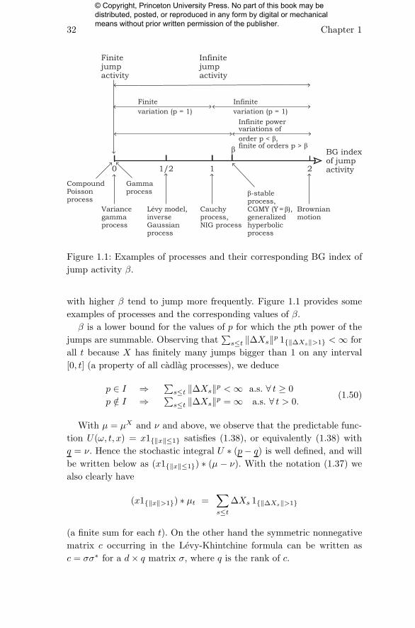
The number β defined above is called the Blumenthal-Getoor index of

the processX , as introduced by Blumenthal and Getoor (1961), precisely

for studying the path properties of Levy processes. Note that, since the

function p 7→ ‖x‖p is decreasing when ‖x‖ ≤ 1, the set I is necessarily

of the form [β,∞) or (β,∞), whereas 2 ∈ I always by (1.23), hence

β ∈ [0, 2].

There is no conflicting notation here: for a stable or tempered sta-

ble process, the stability index and the Blumenthal-Getoor index agree.

Those are examples where I = (β,∞). A gamma process has Blumenthal-

Getoor index β = 0 and again I = (β,∞). For a compound Poisson pro-

cess we have β = 0 and I = [β,∞). More generally, the jumps have finite

activity if and only if 0 ∈ I. Later on, we will see that β can be quite nat-

urally generalized, and interpreted as a jump activity index : processes


32 Chapter 1

Finitejumpactivity

0 1/2 1 2

Infinitejumpactivity

BG indexof jumpactivity

CompoundPoissonprocess

Gammaprocess

Variancegammaprocess

Lévy model,inverseGaussianprocess

Cauchyprocess,NIG process

Finite

variation (p = 1)

Infinite

variation (p = 1)

Infinite powervariations of

order p < β,finite of orders p > β

β-stableprocess,CGMY (Y= β),generalizedhyperbolicprocess

Brownianmotion

β

Figure 1.1: Examples of processes and their corresponding BG index of

jump activity β.

with higher β tend to jump more frequently. Figure 1.1 provides some

examples of processes and the corresponding values of β.

β is a lower bound for the values of p for which the pth power of the

jumps are summable. Observing that∑s≤t ‖∆Xs‖p 1‖∆Xs‖>1 <∞ for

all t because X has finitely many jumps bigger than 1 on any interval

[0, t] (a property of all cadlag processes), we deduce

p ∈ I ⇒ ∑s≤t ‖∆Xs‖p <∞ a.s. ∀ t ≥ 0

p /∈ I ⇒ ∑s≤t ‖∆Xs‖p = ∞ a.s. ∀ t > 0.

(1.50)

With µ = µX and ν and above, we observe that the predictable func-

tion U(ω, t, x) = x1‖x‖≤1 satisfies (1.38), or equivalently (1.38) with

q = ν. Hence the stochastic integral U ∗ (p− q) is well defined, and will

be written below as (x1‖x‖≤1) ∗ (µ − ν). With the notation (1.37) we

also clearly have

(x1‖x‖>1) ∗ µt =∑

s≤t∆Xs 1‖∆Xs‖>1

(a finite sum for each t). On the other hand the symmetric nonnegative

matrix c occurring in the Levy-Khintchine formula can be written as

c = σσ∗ for a d× q matrix σ, where q is the rank of c.



With all this notation, and with b as in (1.24), one can show that

on (Ω,F , (Ft)t≥0,P) there is a q-dimensional Brownian motion W , in-

dependent of the Poisson measure µ, and such that the Levy process X

is

Xt = bt+ σWt + (x1‖x‖≤1) ∗ (µ− ν)t + (x1‖x‖>1) ∗ µt. (1.51)

This is called the Levy-Ito decomposition of X . This decomposition is

quite useful for applications, and also provides a lot of insight on the

structure of a Levy process.

A few comments are in order here:

1. When c = 0 there is no σ, and of course the Brownian motion W

does not show in this formula.

2. The independence of W and µ has been added for clarity, but one

may show that if W and µ are an (Ft)-Brownian motion and an

(Ft)-Poisson measure on some filtered space (Ω,F , (Ft)t≥0,P), then

they necessarily are independent.

3. The four terms on the right in the formula (1.51) correspond to

a canonical decomposition of Xt into a sum of a pure drift term,

a continuous martingale, a purely discontinuous martingale con-

sisting of “small” jumps (small meaning smaller than 1) that are

compensated, and the sum of the “big” jumps (big meaning big-

ger than 1). As we will see, this is also the structure of a general

semimartingale.

4. The four terms in (1.51) are independent of each other; for the last

two terms, this comes from (1.33).

5. These four terms correspond to the decomposition of the charac-

teristic function (1.24) into four factors, that is,

E(eiu

∗Xt

)=

4∏

j=1

φj(u),

whereφ1(u) = eiu

∗bt, φ2(u) = e−12 tu

∗cu,

φ3(u) = et∫‖x‖≤1(e

iu∗x−1−iu∗x)F (dx),

φ4(u) = et∫‖x‖>1(e

iu∗x−1)F (dx).

The terms φ1 and φ2 are the characteristic functions of bt and

σWt, and the last one is the characteristic function of the com-

pound Poisson variable which is the last term in (1.51). For the


34 Chapter 1

third factor, one can observe that on the one hand the variable

(x1(1/n)<‖x‖≤1) ∗ (µ− ν)t is a compound Poisson variable minus

t∫(1/n)<‖x‖≤1 xF (dx), whose characteristic function is

exp t

∫

(1/n)<‖x‖≤1

(eiu

∗x − 1− iu∗x)F (dx),

whereas on the other hand it converges to the third term in (1.51)

as n→ ∞ by the dominated convergence theorem in (1.40).

6. Instead of truncating jumps at 1 as in (1.51), we can decide to

truncate them at an arbitrary fixed ε > 0, in which case the de-

composition formula becomes

Xt = bεt+ σWt + (x1‖x‖≤ε) ∗ (µ− ν)t + (x1‖x‖>ε) ∗ µt

with the drift term changed to

bε = b+

∫x(1‖x‖≤ε − 1‖x‖≤1

)F (dx).

We can more generally employ a truncation function h(x) in lieu of

1‖x‖≤ε, as long as h(x) = 1+ o(‖x‖) near 0 and h(x) = O(1/|x|)near ∞, so that

eiu∗x − 1− iu · xh(x) = O(‖x‖2) as x→ 0

eiu∗x − 1− iu · xh(x) = O(1) as ‖x‖ → ∞

and∫(‖x‖2 ∧ 1)F (dx) <∞ ensures that

∫ ∣∣ eiu∗x − 1− iu∗xh(x)∣∣F (dx) <∞.

The drift needs again to be adjusted to

bh = b+

∫x(h(x)− 1‖x‖≤1

)F (dx)

Different choices of ε or h do not change (c, F ) but they are re-

flected in the drift bh, which is therefore a somewhat arbitrary

quantity. Since the choice of truncation is essentially arbitrary, so

is the distinction between small vs. big jumps. The only distin-

guishing characteristic of big jumps is that there are only a finite

number of them, at the most.



7. Recall that the reason we cannot simply take x ∗ µt is that, whenthe process has infinite jump activity, the series x∗µt =

∑s≤t∆Xs

may be divergent even though the number of jumps is at most

countable. The variable (x1‖x‖>ε) ∗ µt =∑s≤t∆Xs 1‖∆Xs‖>ε,

being a finite sum for all ε > 0, is well defined, but its limit as ε→ 0

may not exist because of the infinitely many jumps. Compensat-

ing solves that problem and (x 1ε<‖x‖≤1) ∗ (µ− ν)t converges as

ε → 0. On the other hand, we cannot simply compensate without

truncating and take x ∗ (µ − ν)t, because (x 1‖x‖>1) ∗ νt may be

divergent; hence the solution which consists in breaking the sum

(or integrals) into two parts, compensated small jumps, and un-

compensated large jumps, both of which are convergent.

8. If the process has finite variation, that is, if ‖x‖ ∗ µt < ∞ almost

surely for all t, or equivalently if∫(‖x‖ ∧ 1)F (dx) < ∞ (note the

absence of a square on ‖x‖), then the integral x ∗ µt is convergent,and the compensation is not needed. The difference between the

representation

Xt = b′t+ σWt + x ∗ µtand (1.51) for a finite variation process consists in a change of drift

from b to b′.

1.3 Semimartingales

1.3.1 Definition and Stochastic Integrals

We now reach the main topic of this chapter. Among all processes, the

class of semimartingales plays a very special role. For example they are

the most general processes with respect to which a (stochastic) inte-

gration theory, having the usual “nice” properties like a Lebesgue con-

vergence theorem, can be constructed. This fact may even be used as

the definition of semimartingales, according to the Bichteler-Dellacherie-

Mokobodski theorem. In mathematical finance they also play a special

role, since one of the most basic results (the so-called fundamental as-

set pricing theorem) says that if no arbitrage is allowed, then the price

process should be a semimartingale.

Definition 1.13. A real-valued process X on the filtered probability space

(Ω,F , (Ft)t≥0,P) is called a semimartingale if it can be written as

X = A+M, (1.52)


36 Chapter 1

where M is a local martingale and A is an adapted cadlag process “with

finite variation,” which means that the total variation of each path t 7→At(ω) is bounded over each finite interval [0, t].

Intuitively, the finite variation process plays the role of a “drift” term

(such as∫ t0 bsds) whereas the local martingale part is “pure randomness”

(such as∫ t0 σsdWs). A deterministic process is a semimartingale if and

only if it has finite variation. This decompositionX =M+A is essentially

not unique, since we can always add to A and subtract fromM the same

martingale with finite variation. Both A and M may be discontinuous.

A d-dimensional semimartingale X = (X i)1≤i≤d is a process whose

components are real-valued semimartingales. A semimartingale is always

adapted and cadlag. Every adapted process of finite variation (e.g. Pois-

son or pure drift) is a semimartingale. Every martingale (e.g. Brownian

motion) is a semimartingale. By virtue of the Levy-Ito decomposition

(1.51), any Levy process is a semimartingale, since it is the sum of a

square integrable martingale and a finite variation process: one may for

example take At = bt+ (x1‖x‖>1) ∗ µt to get a decomposition (1.52).

Now we introduce stochastic integrals with respect to a semimartin-

gale X , starting with the one-dimensional case. Exactly as for the Brow-

nian motion, and substituting W with X , one may define the integral∫ t0 HsdXs by (1.7) for any simple process H of the form (1.6).

Again as for the Brownian motion, this elementary integral can be

extended to a much larger class of integrands. An important difference

with the Brownian case is the fact that we need the integrand to be

predictable, a fundamental requirement without which the whole theory

breaks down. More precisely, we consider processes H with the following

properties:

H is predictable, and locally bounded in the sense that

we have |Ht(ω)| ≤ n for all 0 < t ≤ Tn(ω),

where (Tn) is a sequence of stopping times increasing to ∞.

(1.53)

This is not the largest possible class of integrands, but it will be sufficient

for our purposes. The extension is of course still denoted by∫ t0 HsdXs or

H •Xt, and is uniquely defined up to a null set again. It has properties



analogous to (1.9):

• the process H •Xt is a semimartingale starting at 0

• if X is a local martingale, then so is H •X• the maps H 7→ H •X and X 7→ H •X are linear

• we have a “dominated convergence theorem”:

if Hn → H pointwise and |Hn| ≤ H ′

where H ′ satisfies (1.53), then Hn •X u.c.p.=⇒ H •X.

(1.54)

When X is d-dimensional, one can integrate componentwise a d-

dimensional predictable locally bounded process H = (Hi)1≤i≤d, thus

getting the following one-dimensional process:

H •Xt =

∫ t

0Hs dXs =

d∑

i=1

∫ t

0His dX

is.

Why the predictability requirement? There are two reasons. A first

“mathematical” reason is that, for a general semimartingale, it is im-

possible to extend integrals of simple integrands to all cadlag adapted

processes while preserving the dominated convergence theorem. Second,

in financial applications, trading strategies must be predictable to avoid

arbitrage opportunities. Imagine an investor trading an asset with price

process X at times Ti, 0 = T0 < T1 < · · · < Tn+1 = T , and holding

HTi shares of the asset between Ti and Ti+1. The capital gain from that

strategy isn∑

i=0

HTi (XTi+1 −XTi) =

∫ T

0HtdXt.

The transaction times Ti may be fixed, or more generally they may be

non-anticipating random times (that is, stopping times). For example

the investor may trade the first time X crosses a barrier: this would be

a limit order. Also, HTi is chosen based on information known at Ti: it

is FTi-measurable. The investor’s holdings at each time t are given by

Ht = H010(t) +n∑

i=0

HTi1(Ti,Ti+1](t).

The investor decides to trade at Ti; immediately afterwards, the portfolio

changes from HTi−1 to HTi . Therefore Ht is left-continuous with right-

limits (caglad). This makes it a predictable process.

Trading strategies must be predictable when jumps are present, oth-

erwise there may be arbitrage opportunities. Consider for example Xt =

λt − Nt, where N is a Poisson process with intensity λ. Let T1 denote


38 Chapter 1

the time of the first jump. At that time, X jumps by −1. Consider the

strategy that buys 1 unit of the asset at time 0 for price X0 = 0 and sells

it right before the crash at T1. H is not a predictable process, since it is

impossible to implement this strategy without knowing ahead the time

when T1 will happen. The holdings Ht are given by 1 between [0, T1).

The fact that the interval is open on the right means that this strategy is

not predictable because of the properties of the jump times of a Poisson

process. The strategy generates sure profits since

∫ t

0HsdXs =

λt for t < T1λT1 for t ≥ T1

and does that with zero initial investment, so it is an arbitrage. This

explains why, in the presence of jumps, only predictable strategies are

admissible.

1.3.2 Quadratic Variation

For defining the quadratic variation, one needs to recall some proper-

ties. The first is that a local martingale M can always be written as

Mt =M0+Mct +M

dt , whereM

c0 =Md

0 = 0 and M c is a continuous local

martingale, and Md is a local martingale orthogonal to each continuous

(local) martingale. The second is that a local martingale starting from

0, which has bounded variation in the sense explained after (1.52), and

which is continuous, is almost surely vanishing everywhere. Therefore, if

we consider two decompositions X = M + A = M ′ + A′ as (1.52), then

necessarily M c =M ′c a.s. In other words, we can write the semimartin-

gale X as

Xt = X0 +Xct +Mt +At,

where A0 = M0 = 0 and where A is of finite variation and M is a

local martingale orthogonal to all continuous martingales, and Xc is a

continuous local martingale starting at 0. In this decomposition the two

processes M and A are still not unique, but the process Xc is unique

(up to null sets), and it is called the continuous martingale part of X

(although it usually is a local martingale only). When X is d-dimensional,

so are Xc, M and A, and the components of Xc are denoted X i,c.

Now, we saw in Subsection 1.1.2 that, when two continuous local mar-

tingales M and M ′ are stochastic integrals with respect to a (possibly

multidimensional) Brownian motion, one can define the quadratic covari-

ation (or variation, if M ′ =M). The same is true of all continuous local

martingales: based on the Doob-Meyer decomposition of submartingales



again, we have a unique (up to null sets) continuous adapted process

〈M,M ′〉 starting at 0, with finite variation, and such that

MM ′ − 〈M,M ′〉 is a local martingale,

and further 〈M,M〉 is increasing.At this point, we can introduce the quadratic variation of a one-

dimensional semimartingale X as being

[X,X ]t = 〈Xc, Xc〉t +∑

s≤t(∆Xs)

2. (1.55)

The sum above makes sense, since it is a sum of positive numbers on

the countable set s : ∆Xs 6= 0 ∩ [0, t]. What is not immediately

obvious is that it is a.s. finite, but this fact is one of the main prop-

erties of semimartingales. Hence the process [X,X | is increasing and

cadlag, and also adapted (another intuitive but not mathematically ob-

vious property). Another name for [X,X ] is the “square bracket.” Note

that [X,X ] = 〈X,X〉 when X is a continuous local martingale, and in

general [Xc, Xc] = 〈Xc, Xc〉 is the “continuous part” of the increasing

process [X,X ] (not to be confused with its “continuous martingale part,”

which is identically 0).

For example, if Xt = σWt, where W is Brownian motion, then

[X,X ]t = σ2t. So [X,X ]t is not random, and coincides with the variance

of Xt. This is not the case in general: [X,X ]t, unlike the variance, is a

random variable. It is not defined by taking expectations. For example,

for a Poisson process, since N jumps by 1 whenever it does, [N,N ]t = Ntis the number of jumps of the process between 0 and t, and we also have

[X,X ]t = Nt for the martingale Xt = Nt−λt if λ is the parameter of the

Poisson process N . Moreover, [X,X ]t is well defined for all semimartin-

gales, including those with infinite variance.

If now X and X ′ are two real-valued semimartingales we set

[X,X ′]t = 〈Xc, X ′c〉t +∑

s≤t∆Xs∆X

′s. (1.56)

Here again the sum above is a.s. absolutely convergent, by the finiteness

in (1.55) for X and X ′ and the Cauchy-Schwarz inequality. The process

[X,X ′] is adapted and of finite variation, but not necessarily increasing

any more, and is called the quadratic covariation process of X and X ′.

For example, if Xt =∫ t0 σsdWs and X ′

t =∫ t0 σ

′sdW

′s, where W and W ′

are two Brownian motions with correlation coefficient ρ, then [X,X ′]t =∫ t0 ρσsσ

′s ds.


40 Chapter 1

For any real a and any other semimartingale X ′′ we have

[X + aX ′, X ′′] = [X,X ′′] + a[X ′, X ′′], [X,X ′] = [X ′, X ].

Another useful property, which immediately follows from this, is the po-

larization identity:

[X,X ′] =1

4

([X +X ′, X +X ′]− [X −X ′, X −X ′]

)(1.57)

which expresses the quadratic covariation in terms of quadratic variations

only. Finally, the following is obvious:

[X,X ′] = [X −X0, X′ −X ′

0]. (1.58)

When X is d-dimensional, we thus have a d × d matrix-valued process

[X,X ] = ([X i, Xj])1≤i,j≤d. For all s, t ≥ 0 the matrix [X,X ]t+s− [X,X ]tis symmetric nonnegative.

We end this subsection with a set of inequalities, known under

the name of Burkholder-Gundy inequalities when p > 1 and Davis-

Burkholder-Gundy when p = 1 (when p = 2 it is also a version of Doob’s

inequality). These inequalities assert that, if X is a local martingale and

p ≥ 1 and S ≤ T are two arbitrary stopping times, then

E(sups∈[S,T ] |XS+s −Xs|p | FS

)

≤ Kp E(([X,X ]T − [X,X ]S)

p/2 | FS),

(1.59)

whereKp is a universal constant depending on p only, and [X,X ]T stands

on the set T = ∞ for the increasing (possibly infinite) limit of [X,X ]tas t increases to infinity, and [X,X ]T − [X,X ]S = 0 on the set where

S = T = ∞. As a matter of fact, we also have the inequality (1.59) in

the other direction, and with another constant Kp, but this will not be

useful for us.

1.3.3 Ito’s Formula

We are now ready to state the general form of Ito’s formula, which ex-

tends (1.15). From their very definition, semimartingales form a vector

space; linear combinations of a finite number of semimartingales are semi-

martingales. But the class of semimartingales is closed under much more

general transformations, and much of its usefulness comes from this fact.

If f is a C2 function on Rd and X is a d-dimensional semimartingale, the



process Y = f(X) is also a semimartingale and is given by

f(Xt) = f(X0) +d∑

i=1

∫ t

0f ′i(Xs−) dX

is

+1

2

d∑

i,j=1

∫ t

0f ′′ij(Xs−) d〈X i,c, Xj,c〉s (1.60)

+∑

s≤t

(f(Xs)− f(Xs−)−

d∑

i=1

f ′i(Xs−)∆X

is

).

The reader will notice that all processes f ′i(Xt−) and f ′′

ij(Xs−) are left-

continuous with right limits, so they are locally bounded and predictable

and the first (stochastic) and second (ordinary) integrals make sense.

Moreover, the sth summand in the last sum is smaller than Kn‖∆Xs‖2on the set sups≤t ‖Xs‖ ≤ n, for a constant Kn. Since

∑s≤t ‖∆Xs‖2 <

∞ (because the quadratic variation is finite), this last sum is in fact

absolutely convergent. In other words, all terms on the right of (1.60) are

well defined.

We end this subsection with the promised proof of (1.14), in the gen-

eral setting of semimartingales. The result is stated in the form of a theo-

rem, which is unusual in this chapter but motivated by its importance in

the econometrics literature and more generally for high-frequency statis-

tics.

Theorem 1.14. Let X and X ′ be two semimartingales. For each n, let

T (n, 0) = 0 < T (n, 1) < T (n, 2) < · · · be a strictly increasing sequence

of stopping time with infinite limit, and suppose that the mesh πn(t) =

supi≥1(T (n, i) ∧ t− T (n, i− 1) ∧ t) goes to 0 for all t, as n → ∞. Then

we have the following convergence in probability:

∑i≥1

(XT (n,i)∧t −XT (n,i−1)∧t

)(X ′T (n,i)∧t −X ′

T (n,i−1)∧t)

u.c.p.

=⇒ [X,X ′]t.(1.61)

Moreover, for any given t we also have

∑i≥1, T (n,i)≤t

(XT (n,i) −XT (n,i−1)

)(X ′T (n,i) −X ′

T (n,i−1)

)

P−→ [X,X ′]t.(1.62)

in restriction to the set ∆Xt = 0 ∪ ∆X ′t = 0 on which either X or

X ′ have no jump at time t, and on the whole set Ω when further, for any

n, there is an index i such that T (n, i) = t.


42 Chapter 1

The convergence (1.62) may actually fail on the set ∆Xt 6= 0,∆X ′t 6=

0. For example, if for all n there is no i such that T (n, i) = t, the left

side of (1.62) converges in probability (on Ω) to the left limit [X,X ′]t−,

which equals [X,X ′]t −∆Xt∆X′t.

The theorem (and its proof below) assumes that πn(t) → 0 pointwise,

but the condition πn(t)P−→ 0 is indeed enough for the results to hold.

Proof. In view of (1.58) we can replaceX andX ′ by X−X0 and X′−X ′

0,

or equivalently assume that X0 = X ′0 = 0. The proof is based on the

elementary equality (x− y)(x′ − y′) = xx′ + yy′ − y(x′ − y′)− y′(x− y)

applied with x = XT (n,i)∧t and y = XT (n,i−1)∧t and x′ = X ′

T (n,i)∧t and

y′ = X ′T (n,i−1)∧t. Summing over all i ≥ 1, we deduce that the left side of

(1.61) is equal to

XtX′t −

∫ t

0Hns dX

′s +

∫ t

0H ′ns dXs

(recall X0 = X ′0 = 0), where we have set

Hns =

∑

i≥1

XT (n,i−1) 1(T (n,i−1),T (n,i)](s)

and a similar formula for H ′ns , with X ′ instead of X . The processes Hn

are adapted and left-continuous, hence predictable, and |Hn| ≤ Z where

Z is the predictable locally bounded process defined by Zs = sup(|Xr| :r ∈ [0, s)). Moreover, since the mesh of the subdivision goes to 0, we

have Hn → X− pointwise. Then the dominated convergence theorem

for stochastic integrals, see (1.54), yields Hn • X ′ u.c.p.=⇒ X− • X ′, and

H ′n •X u.c.p.=⇒ X ′

− •X holds by the same argument. In other words, the

left side of (1.61) converges in the u.c.p. sense to

XtX′t −

∫ t

0Xs− dXs +

∫ t

0X ′s− dXs.

It remains to apply Ito’s formula to the two-dimensional semimartingale

with components X and X ′ and the function f(x, x′) = xx′: we deduce

from (1.56) that the above expression is equal to [X,X ′]t, and thus (1.61)

is proved. When for each n there is i such that T (n, i) = t, the left sides

of (1.61) and (1.62) are the same, so (1.62) is proved. Finally, in general,

the difference between the left sides of (1.61) and (1.62) is smaller than

ρ(ε) = sup(|Xt −Xt−s| |X ′t −X ′

t−s| : s ∈ [0, ε]) as soon as πn(t) ≤ ε. On

the set ∆Xt = 0 ∪ ∆X ′t = 0 we have ρ(ε) → 0 as ε → 0. Then the

convergence (1.62) in restriction to this set readily follows from the fact

that πn(t) → 0.



1.3.4 Characteristics of a Semimartingale and the

Levy-Ito Decomposition

Here, X is a d-dimensional semimartingale on (Ω,F , (Ft)t≥0,P), and we

are now almost ready to define the characteristics of X .

The process∑s≤t∆Xs 1‖∆Xs‖>1, or equivalently (x1‖x‖>1) ∗ µ

where µ = µX is the jump measure of X defined by (1.36), is of finite

variation. Then we can rewrite (1.52) as

Xt = X0 +A′t +Mt +

∑

s≤t∆Xs 1‖∆Xs‖>1

where M0 = A′0 = 0 and A′ is of finite variation and M is a local

martingale. Now, one can show that the semimartingale A′ +M , which

has jumps smaller than 1 by construction, can be written in a unique (up

to null sets) way as A′ +M = B +N , where again N0 = B0 = 0 and N

is a local martingale and B is a predictable process of finite variation.

Definition 1.15. The characteristics of the semimartingale X are the

following triple (B,C, ν):

(i) B = (Bi)1≤i≤d is the predictable process of finite variation defined

above;

(ii) C = (Cij)1≤i,j≤d is the quadratic variation of the continuous local

martingale part Xc of X, that is, Cij =⟨X i,c, Xj,c

⟩;

(iii) ν is the (predictable) compensating measure of the jump measure

µ = µX of X, as defined in (1.41).

Sometimes one says “predictable characteristics” or “local character-

istics” of the semimartingale X . The name comes from the fact that,

when X is a Levy process with characteristics triple (b, c, F ), then its

characteristics in the semimartingale sense are

Bt(ω) = bt, Ct(ω) = ct, ν(ω, dt, dx) = dt⊗ F (dx). (1.63)

So (B,C, ν) and (b, c, F ) convey the same information. Note that in this

case the characteristics (B,C, ν) are not random. This turns out to be

“necessary and sufficient.” More precisely, a semimartingale X has non-

random characteristics if and only if it has (Ft)-independent increments;

and it has characteristics of the form (1.63) if and only if it is an (Ft)-Levy process.

The reader should not be misled: unlike for Levy processes (or more

generally for processes with independent increments), the characteristics

do not characterize the law of the process in general. Whether they do


44 Chapter 1

characterize the law in specific cases is an important problem, closely

related to the uniqueness of (weak) solutions of some associated SDEs,

and we will come back to this point later.

Now, although the characteristics do not always characterize the pro-

cess X , they provide useful information, especially on the jumps. For

example, we have a (partial) analogue of (1.48): for any nonnegative

Borel function g on Rd with g(0) = 0 and any t > 0,

the two sets (g ∧ 1) ∗ νt <∞ and g ∗ µt <∞are a.s. equal

(1.64)

and in particular, similar to (1.50), for any p ≥ 0 we have

the two sets (‖x‖p ∧ 1) ∗ νt <∞and

∑s≤t ‖∆Xs‖p <∞

are a.s. equal.

(1.65)

The triple (B,C, ν) satisfies a number of structural properties, coming

from its definition. The process C is such that Ct+s −Ct is a symmetric

nonnegative d × d matrix, as already mentioned. Next, B and ν are

predictable, with finite variation for B, but there are other necessary

requirements, namely there is a version of (B, ν) satisfying identically

(‖x‖2 ∧ 1) ∗ νt(ω) <∞, ν(ω, t × Rd) ≤ 1,

‖∆Bt(ω)‖ ≤ 1, ν(ω, t × Rd) = 0 ⇒ ∆Bt(ω) = 0.(1.66)

The analogy with Levy processes goes further; for example we have a

formula similar to the Levy-Ito decomposition, that is,

Xt = X0 +Bt +Xct + (x 1‖x‖≤1) ∗ (µ− ν)t + (x 1‖x‖>1) ∗ µt, (1.67)

where the stochastic integral above makes sense because of the first prop-

erty in (1.66). However, this may look like (1.51), but µ is not a Poisson

measure and Xc is not a Brownian motion here.

1.4 Ito Semimartingales

1.4.1 The Definition

As seen above, quite a few properties of Levy processes extend to gen-

eral semimartingales, but there are also big differences, like the fact that

ν(ω, t×Rd) may be positive. There is, however, a class of semimartin-

gales which is a more direct extension of Levy processes:



Definition 1.16. A d-dimensional semimartingale X is an Ito semi-

martingale if its characteristics (B,C, ν) are absolutely continuous with

respect to the Lebesgue measure, in the sense that

Bt =

∫ t

0bsds, Ct =

∫ t

0csds, ν(dt, dx) = dt Ft(dx), (1.68)

where b = (bt) is an Rd-valued process, c = (ct) is a process with values in

the set of all d× d symmetric nonnegative matrices, and Ft = Ft(ω, dx)

is for each (ω, t) a measure on Rd. The terms (bt, ct, Ft) are called the

spot characteristics of X.

These bt, ct and Ft necessarily have some additional measurability

properties, so that (1.68) makes sense: we may choose bt and ct pre-

dictable (or simply progressively measurable, this makes no difference in

the sequel and does not change the class of Ito semimartingales), and Ftis such that Ft(A) is a predictable process for all A ∈ Rd (or progressively

measurable, again this makes no difference). The last three requirements

of (1.66) are automatically fulfilled here, and we can and will choose a

version of Ft which satisfies identically

∫(‖x‖2 ∧ 1) Ft(ω, dx) < ∞

and∫ t0 ds

∫(‖x‖2 ∧ 1) Ft(ω, dx) < ∞.

(1.69)

In view of (1.63), any Levy process is an Ito semimartingale.

There is an apparent contradiction between Definitions 1.1 and 1.16:

a continuous Ito semimartingale in the former sense (or Brownian semi-

martingale) is also Ito in the latter sense, but the converse is not obvious

when X is continuous. However, this contradiction is only apparent.

To be more specific, assume for example that d = 1 and that X is

continuous, and an Ito semimartingale in the sense of (1.16), and also

that Bt = 0 identically, so X = Xc. The question becomes: can we find

a Brownian motion W and a progressively measurable process H such

that Xt =∫ t0 HsdWs ? If this is the case, we necessarily have H2

t = ct, so

since we know that ct ≥ 0, natural candidates are

Ht =√ct, Wt =

∫ t

0

1

HsdXs.

Of course the second integral does not make sense if ct vanishes some-

where, and it should thus be replaced by

Wt =

∫ t

0

1

Hs1Hs 6=0 dXs.


46 Chapter 1

This defines a continuous martingaleW starting at 0, and with quadratic

variation∫ t0 1cs>0 ds, which may be different from t: hence W is not

necessarily a Brownian motion; when for example ct = 0 for all t ≤ 1 it

is quite possible that the σ-field F1 is trivial and thus there simply does

not exist any (Ft)-Brownian motion on (Ω,F , (Ft)t≥0,P).

The solution to this problem needs an extension of the original prob-

ability space. The need for an extension also arises in other contexts in

this book, so we devote the next subsection to the general question of

“extending” the probability space.

1.4.2 Extension of the Probability Space

The space (Ω,F , (Ft)t≥0,P) is fixed. Let (Ω′,F ′) be another measurable

space, and Q(ω, dω′) be a transition probability from (Ω,F) into (Ω′,F ′).

We can define the products

Ω = Ω× Ω′, F = F ⊗ F ′, P(dω, dω′) = P(dω)Q(ω, dω′). (1.70)

The probability space (Ω, F , P) is called an extension of

(Ω,F , (Ft)t≥0,P). Any variable or process which is defined on ei-

ther Ω or Ω′ is extended in the usual way to Ω, with the same symbol;

for example Xt(ω, ω′) = Xt(ω) if Xt is defined on Ω. In the same way, a

set A ⊂ Ω is identified with the set A×Ω′ ⊂ Ω, and we can thus identify

Ft with Ft ⊗ ∅,Ω′, so (Ω, F , (Ft)t≥0, P) is a filtered space.

The filtration (Ft) on the extended space does not incorporate any

information about the second factor Ω′. To bridge this gap we consider

a bigger filtration (Ft)t≥0 on (Ω, F), that is with the inclusion property

Ft ⊂ Ft, ∀t ≥ 0.

The filtered space (Ω, F , (Ft)t≥0, P) is then called a filtered extension of

(Ω,F , (Ft)t≥0,P).

In many, but not all cases the filtration (Ft) has the product form

Ft = ∩s>t Fs ⊗F ′s (1.71)

where (F ′t) is a filtration on (Ω′,F ′). Quite often also, the transition prob-

ability Q has the simple form Q(ω, dω′) = P′(dω′) for some probability

on (Ω′,F ′). In the latter case we say that the extension is a product ex-

tension, and if further (1.71) holds we say that we have a filtered product

extension, which is simply the product of two filtered spaces.



A filtered extension is called very good if it satisfies

ω 7→∫1A(ω, ω

′)Q(ω, dω′) is Ft-measurable

for all A ∈ Ft, all t ≥ 0.(1.72)

Under (1.71), this is equivalent to saying that ω 7→ Q(ω,A′) is Ft-measurable for all A′ ∈ F ′

t and t ≥ 0. A very good filtered extension

is very good because it has the following nice properties:

• any martingale, local martingale, submartingale,

supermartingale on (Ω,F , (Ft)t≥0,P)

is also a martingale, local martingale, submartingale,

supermartingale on (Ω, F , (Ft)t≥0, P)

• a semimartingale on (Ω,F , (Ft)t≥0,P)

is a semimartingale on (Ω, F , (Ft)t≥0, P),

with the same characteristics.

(1.73)

Statement (1.72) is equivalent to saying that any bounded martingale

on (Ω,F , (Ft)t≥0,P) is a martingale on (Ω, F , (Ft)t≥0, P). For example

a Brownian motion on (Ω,F , (Ft)t≥0,P) is also a Brownian motion on

(Ω, F , (Ft)t≥0, P) if the extension is very good, and the same for Poisson

random measures.

Many extensions are not very good: for example take Q(ω, .) to be

the Dirac mass εU(ω), on the space (Ω′,F ′) = (R,R) endowed with the

filtration F ′t = F ′ for all t, and where U is an R-valued variable on

(Ω,F) which is not measurable with respect to the P-completion of F1,

say. Then Q(ω,A′) = 1A′(U(ω)) is not F1-measurable in general, even

when A′ ∈ F ′1, and the extension is not very good.

1.4.3 The Grigelionis Form of an Ito Semimartingale

We are now ready to give our representation theorem. The difficult part

comes from the jumps of our semimartingale, and it is fundamentally a

representation theorem for integer-valued random measure in terms of a

Poisson random measure, a result essentially due to Grigelionis (1971).

The form given below is Theorem (14.68) of Jacod (1979), and we will call

the representation given here the Grigelionis form of the semimartingale

X .

We have the d-dimensional Ito semimartingale X with characteristics

(B, c, ν) given by (1.68). Moreover, d′ is an arbitrary integer with d′ ≥ d,

and E is an arbitrary Polish space with a σ-finite and infinite measure


48 Chapter 1

λ having no atom, and q(dt, dx) = dt ⊗ λ(dx). Then one can construct

a very good filtered extension (Ω, F , (Ft)t≥0, P), on which are defined a

d′-dimensional Brownian motion W and a Poisson random measure p on

R+ × E with intensity measure λ, such that

Xt = X0 +∫ t0 bsds+

∫ s0 σsdWs

+(δ1‖δ‖≤1) ⋆ (p− q)t + (δ1‖δ‖>1) ⋆ pt,(1.74)

where σt is an Rd ⊗ Rd′

-valued process on (Ω,F , (Ft)t≥0,P) which is

predictable (or only progressively measurable), and δ is a predictable

Rd-valued function on Ω×R+×E, both being such that the integrals in

(1.74) make sense.

The process bt is the same here and in (1.68), and we have close

connections between (σt, δ(t, z)) and (ct, Ft). Namely, a version of the

spot characteristics ct and Ft is given by the following:

• ct(ω) = σt(ω)σ⋆t (ω)

• Ft(ω, .) = the image of the measure λ

restricted to the set x : δ(ω, t, x) 6= 0by the map x 7→ δ(ω, t, x).

(1.75)

Conversely, any process of the form (1.74) (with possibly b, σ and

δ defined on the extension instead of (Ω,F , (Ft)t≥0,P)) is an Ito semi-

martingale on (Ω, F , (Ft)t≥0, P), and on (Ω,F , (Ft)t≥0,P) as well if it is

further adapted to (Ft). Therefore, the formula (1.74) may serve as the

definition of Ito semimartingales, if we do not mind extending the space,

and for practical applications we do not mind ! Therefore, in the sequel

we freely use the Grigelionis form above, pretending that it is defined on

our original filtered space (Ω,F , (Ft)t≥0,P).

There is a lot of freedom in the choice of the extension, of the space E

and the function δ, and even of the dimension d′ and the process σ: for the

latter, for example, the requirement being σtσ⋆t = ct, we can always take

an arbitrary d′ ≥ d, or more generally a d′ not smaller than the maximal

rank of the matrices ct(ω). A natural choice for E is E = Rd, but this

is not compulsory and we may take in all cases E = R with λ being the

Lebesgue measure. For example, if we have several Ito semimartingales,

and even countably many of them, we can use the same measure p for

representing all of them at once.

For a Levy process, the Grigelionis form coincides with its Levy-Ito

representation, upon taking p = µ and δ(ω, t, x) = x. More generally, in

equation (1.74), the term (δ1‖δ‖≤1) ⋆ (p− q)t corresponds to the small



jumps of the process, while the term (δ1‖δ‖>1) ⋆ pt corresponds to the

big jumps of the process.

1.4.4 A Fundamental Example: Stochastic

Differential Equations Driven by a Levy

Process

We have already mentioned stochastic differential equations (SDE) of the

form (1.18), driven by a Brownian motion. Natural extensions of them

are SDEs driven by a Levy process Z, written as

dXt = a(Xt−) dZt, X0 = Y. (1.76)

Here Z is a q-dimensional Levy process, the “solution” X will be d-

dimensional, so Y is an F0-measurable Rd-valued variable, and a is a

function from Rd into Rd×Rq. As for (1.18), a (strong) solution is a cadlag

adapted process X which satisfies the following, written componentwise:

X it = Y i +

q∑

j=1

∫ t

0a(Xs−)

ij dZjs . (1.77)

The fact that we take the left limit a(Xs−) in the integral above, and

not a(Xs), is absolutely crucial, because the integrand needs to be pre-

dictable, otherwise the stochastic integral a priori makes no sense. Of

course when Z is continuous, hence the solution X as well, we have

a(Xs−) = a(Xs).

Note that (1.18) is a special case of (1.76), although it may not be

apparent at first glance: in (1.18), if W is q′-dimensional, we take q =

q′ + 1 and Zj =W j for j ≤ q′ and Zqt = t, and the coefficient a defined

by aij = σij when j ≤ q′ and aiq = bi.

Here again, a wide variety of conditions on a imply existence and/or

uniqueness of the solution of (1.76). The simplest one is that a is locally

Lipschitz with at most linear growth, but many other conditions exist,

sometimes related with the specific properties of the driving Levy process

Z.

Now, assuming (1.77), the process X is of course a semimartingale,

and even an Ito semimartingale. If (β, γ, F ) is the characteristic triple

of Z, and using the Levy-Ito representation of Z with p = νZ and q =


50 Chapter 1

νX = dt⊗ F (dz) and σ such that σσ∗ = γ, we can rewrite (1.77) as

X it = X i

0 +

q∑

j=1

∫ t

0a(Xs−)

ijβj ds+

q∑

j,k=1

∫ t

0a(Xs−)

ijσjk dW ks

+

q∑

j=1

∫ t

0

∫

Rq

a(Xs−)ijzj 1‖z‖≤1 (p− q)(ds, dz)

+

q∑

j=1

∫ t

0

∫

Rq

a(Xs−)ijzj 1‖z‖>1 p(ds, dz).

Therefore, the characteristics (B,C, ν) of X take the form (1.68) with

the following (where a(x)z stands for the d-dimensional vector with com-

ponents∑qj=1 a(x)

ijzj):

bit =∑qj=1 a(Xt−)ij

(βj+

+∫

Rq zj(1‖z‖≤1 − 1‖a(Xt−)z‖≤1

)F (dz)

)

cijt =∑qk,l=1 a(Xt−)ikγkl a(Xt−)jl

Ft(ω, dx) = the image of the measure F

by the map z 7→ a(Xt−(ω))z.

(1.78)

These characteristics have a complicated form, although they indeed

come naturally as functions of the coefficient a: the problem of find-

ing a process which is an Ito semimartingale with characteristics given a

priori in the form (1.78) reduces in fact to solving Equation (1.76).

Now, we also have, in a somewhat more immediate way, the Grigelionis

form of X , provided we take for W and p the terms coming in the Levy-

Ito decomposition of Z. Namely, in (1.74) the process bt is the same

(complicated) process as above, but σt and δ take the simple form

σikt =

q∑

j=1

a(Xt−)ijσjk, δ(t, z)i =

q∑

j=1

a(Xt−)ijzj.

In fact, equations like (1.68) are not really the most natural ones to

consider in a discontinuous setting. It is also useful to consider equa-

tions which are driven directly by a Brownian motion W and a (general)

Poisson random measure p on R+ × E for some “abstract” space E and

with intensity measure q = dt ⊗ λ(dz). This amounts to considering an



equation of the form

Xt = Y +

∫ t

0b(Xs−)ds+

∫ s

0σ(Xs−)dWs

+

∫ t

0

∫

Ev(Xs−, z)1‖v(Xs−,z)‖≤1 (p− q)(ds, dz) (1.79)

+

∫ t

0

∫

Ev(Xs−, z)1‖v(Xs−,z)‖>1 p(ds, dz),

where b is an Rd-valued function on Rd and σ is an Rd⊗Rq-valued function

on Rd (where q is the dimension of W ) and v is an Rd-valued function on

Rd ×E. This type of equation includes (1.77) and immediately gives the

Grigelionis form of the solution. When existence and uniqueness hold for

all initial conditions Y , the solution is a homogeneous Markov process,

and the restriction of its infinitesimal generator to the C2 functions takes

the form

Af(x) =d∑

i=1

b(x)if ′i(x) +

1

2

d∑

i,j=1

c(x)ijf ′′ij(x)

+

∫

E

(f(x+ v(x, z))− f(x) (1.80)

−d∑

i=1

f ′i(x)v(x, z)

i 1‖v(x,z)‖≤1)λ(dz),

where c = σσ∗. This extends (1.17), and one may show that any homo-

geneous Markov process which is an Ito semimartingale is of this form.

More generally even, one can interpret the Grigelionis form (1.74) as

a generalized SDE similar to (1.79), but with “coefficients” bt(ω), σt(ω)

and δ(ω, t, z) which may depend on the whole past of X before time

t, and also on ω in an arbitrary (predictable) way. In this setting the

infinitesimal generator is replaced by the so-called extended generator

Atf(x) =d∑

i=1

bitf′i(x) +

1

2

d∑

i,j=1

cijt f′′ij(x)

+

∫

E

(f(x+ δ(t, z))− f(x)

−d∑

i=1

f ′i(x)δ(t, z)

i 1‖δ(t,z)‖≤1)λ(dz),

so At is a second order integro-differential operator mapping the C2 func-

tions into the set of random variables. This extended generator is no


52 Chapter 1

longer the generator of a semi-group, but the characteristic martingale

property of the generator is preserved, and it reads as follows: for any C2

function f , the process

Mft = f(Xt)− f(X0)−

∫ t

0Asf ds

is a local martingale.

As a consequence of all these considerations, one may state (in a some-

what heuristic way) that the characteristics (B,C, ν), or equivalently

(and perhaps more appropriately) (bt, ct, Ft), determine the dynamics of

the process. They are thus of fundamental importance for modeling pur-

poses. More precisely, the problem of describing the process X is often

considered as “solved” when one knows the characteristics (B,C, ν), in

connection with X itself and perhaps with other random inputs.

1.5 Processes with Conditionally

Independent Increments

In most problems considered in this book we start with an underlying

process X which is an Ito semimartingale on some given filtered prob-

ability space (Ω,F , (Ft)t≥0,P). We then consider various functionals of

X , such as the approximate quadratic variation defined as the left side of

(1.61) or (1.62). We are interested first in the convergence in probability

of these functionals, as in Theorem 1.14, and ultimately in the rate of

convergence and, whenever possible, in the “second order” asymptotic

behavior, or Central Limit Theorem, associated with the convergence in

probability. As it turns out, the limit when such a CLT holds will almost

always be defined on an extension of (Ω,F , (Ft)t≥0,P), as introduced in

(1.70), and what will be available is the law of the limit under the mea-

sures Q(ω, dω′), or equivalently the F -conditional law of the limit; the

reader can look immediately at Chapter 3 for a (relatively) simple case

for which this situation occurs.

Actually, the putative limits will (almost) always be a stochastic pro-

cess U belonging to a special and relatively restricted class, namely the

processes having F -conditionally independent increments. The aim of

this section is to describe those processes, which have an interest by

themselves and can in fact be defined independently of any limiting pro-

cedure. Toward this aim, we first need to consider processes which extend

Levy processes.



1.5.1 Processes with Independent Increments

A q-dimensional process U defined on a space (Ω,F , (Ft)t≥0,P) is called

a process with independent increments, relative to (Ft), if it is cadlag,

with U0 = 0, adapted, and the increment Ut+s−Ut is independent of Ftfor all s, t ≥ 0. In other words, we have all properties of Definition 1.1

except that the law of Ut+s − Ut may depend on both s and t. When

(Ft) = (FUt ) is the filtration generated by U we simply say a process with

independent increments.

When the increments are stationary, U is simply a Levy process.

Otherwise, it still exhibits similar features. In particular, when it is a

semimartingale, its characteristics relative to (Ft) are deterministic (this

property characterizes semimartingales with independent increments).

We can thus decompose its third (deterministic) characteristic ν as a sum

ν = νc + νd, where, using the notation D = t > 0 : ν(t × Rq) > 0and its complement Dc in R+,

νc(dt, dx) = ν(dt, dx)1Dc(t), νd(dt, dx) =∑

s∈Dεs(dt)⊗ ν(s, dx)

(there is no randomness here). We thus have two types of jumps: those

occurring at a time outside the countable set D, which are like the jumps

of a Levy process except that the associated Poisson measure is non-

homogeneous (it admits νc as its intensity measure), and those occurring

at a time in D, which are called fixed times of discontinuity because we

have

P(∆Ut 6= 0) > 0 ⇐⇒ t ∈ D.

Although it is possible to describe all processes with independent in-

crements, we restrict our attention to those which are encountered as

limits in this book. This class of processes, denoted for short as Lq0 be-

low (q stands for the dimension), is in fact rather special: it is the class

of all processes of the form

Ut =∑

n: tn≤tv(tn)Yn +

∫ t

0v′(s) dW ′

s (1.81)

where

• v is a measurable function on R+, with dimension q ×Q

• v′ is a measurable locally square-integrable function on R+,

with dimension q ×Q′

• W ′ is a Q′-dimensional Brownian motion

• tn ∈ (0,∞], tn 6= tm if n 6= m and tn <∞• the RQ-valued variables Yn are i.i.d. and independent of W ′,


54 Chapter 1

and we suppose that at least one of the following two sets of conditions

holds:

(i) 0 < E(‖Y1‖) <∞ and∑n: tn≤t ‖v(tn)‖ <∞

(ii) E(Y1) = 0, 0 < E(‖Y1‖2) <∞ and∑n: tn≤t ‖v(tn)‖2 <∞.

Under (i) the first sum in (1.81) is absolutely convergent. Under (ii)

this is no longer necessarily true, but it converges in L2 and the resulting

process is a square-integrable martingale. Since P(Yn 6= 0) > 0, the set

of fixed times of discontinuity of U is the set of all finite tn’s such that

v(tn) 6= 0.

The following (obvious) fact is important:

Any U in Lq0 has independent increments, and its law is

determined by the functions v and v′, the set

D = tn : n ≥ 1 ∩ (0,∞), and the law η of the variables Yn,

(1.82)

and we can relabel the sequence tn at will. Finally, under the previous

conditions we have, relative to the filtration (FUt ) generated by U :

• U is a centered Gaussian process

⇔ either η is a centered Gaussian law or v = 0 on D

• U is a continuous centered Gaussian martingale

⇔ v = 0 on D.

(1.83)

1.5.2 A Class of Processes with F-Conditionally

Independent Increments

Generally speaking, a q-dimensional process U on an extension (Ω, F , P)of the original probability space (Ω,F ,P), see (1.68), is called a process

with F-conditionally independent increments if, for P-almost all ω, it is

a process with independent increments under the measure Q(ω, .).

As previously, we restrict our attention to those U which, under

Q(ω, .), belong to the class Lq0 described above, and we even suppose

that the law η (as in (1.82)) is the same for all ω. Therefore, in order to

construct such a process, we start with the following ingredients:

• a progressively measurable process V with dimension q ×Q

• a progressively measurable, locally square-integrable

process V ′ with dimension q ×Q′

• a probability measure η on RQ

• a sequence Tn of stopping times, with Tn 6= Tmon the set Tn <∞ if n 6= m.



We also suppose that V and η satisfies at least one of the following two

conditions:

(i) 0 <∫‖x‖ η(dx) <∞ and

∑n:Tn≤t ‖VTn‖ <∞

(ii) 0 <∫‖x‖2 η(dx) <∞,

∫x η(dx) = 0,

and∑n:Tn≤t ‖VTn‖2 <∞.

(1.84)

The construction of a version of the process U is now quite simple. We

choose an extra space (Ω′,F ′,P′) endowed with the following objects:

• a q′-dimensional Brownian motion W ′

• a sequence (Yi)i≥1 of i.i.d. variables,

independent of W ′, with law η.

(1.85)

Then we define the product extension

Ω = Ω× Ω′, F = F ⊗ F ′, P = P ⊗ P′. (1.86)

We also consider the smallest filtration (Ft)t≥0 on Ω which contains

(Ft)t≥0 (recall that any variable on Ω or Ω′ can be considered as a vari-

able on the product Ω, so Ft is also a σ-field on Ω), and to which W ′

is adapted, and such that each Yn is FTn -measurable. Due to the inde-

pendence built in (1.85) and (1.86), the process W ′ is an (Ft)-Brownianmotion and the processes V, V ′ are (Ft)-progressively measurable. Then

it is an easy job to prove that the next formula defines a process U on

the extension, with all the required properties:

Ut =∑

n:Tn≤tVTn Yn +

∫ t

0V ′s dW

′s. (1.87)

It is useful to have explicit formulas for the conditional first and second

moments of the process U in this setting. Letting

Mj =∫xjη(dx), Mjk =

∫xjxkη(dx),

C′jkt =

∑q′

l=1

∫ t0 V

′jls V ′kl

s ds,(1.88)

we get

(1.84)-(i) ⇒ E(U jt | F) =∑s≤t∑qk=1 V

jks Mk

(1.84)-(ii) ⇒

E(U jt | F) = 0

E(U jt Ukt | F) = C′jk

t

+∑s≤t∑ql,m=1 V

jls V

kms Mlm.


56 Chapter 1

Finally, if D(ω) = Tn(ω) : n ≥ 1 ∩ (0,∞), the next two equivalences

follow from (1.83):

• U is F -conditionally a centered Gaussian process

⇔ η is centered Gaussian or V = 0 on D

• U is F -conditionally a continuous

centered Gaussian martingale ⇔ V = 0 on D.

(1.89)

We conclude with an important particular case. In many instances,

the process U given by (1.87) is continuous, that is, Ut =∫ t0 V

′s dW

′s. The

law of a continuous centered process U with independent increments is

completely specified by its covariance matrix E(U itUjt ), as a function of

time. This is of course still true when U is continuous, with F -conditional

mean 0 and with F -conditionally independent increments. That is, the

F -conditional law of U in this case is completely specified by the process

C′ given in (1.88).

In practice, one usually goes the other way around: one starts with a

q × q-dimensional process C′ of the form

C′t =

∫ t

0c′s ds,

with c′ adapted, with values in the set of nonnegative symmetric q × q

matrices. Then, what precedes gives us a process U which is continuous

and F -conditionally centered and with independent increments (equiv-

alently: F -conditionally a centered Gaussian martingale). For this, it

suffices to choose a q × Q-dimensional process V which is adapted and

is a square root of c′, that is, c′t = VtV∗t ; this is always possible by a

measurable selection theorem, up to null sets, and with any choice of Q

with Q ≥ q, or even with Q ≥ supω,t rank(c′t(ω)).


from diﬀusions to semimartingales

Documents