frequently asked questions pertaining to tariff - nersa
TRANSCRIPT
Frequently Asked Questions (FAQ):
Tariff Methodology for the Setting and Approval of Tariffs in the
Petroleum Pipelines Industry
Version 4
Approved on
29 July 2013

FAQ Version 4: Approved on 29 July 2013.
Page 1 of 59
Frequently Asked Questions (FAQ):
Tariff Methodology for the Setting and Approval of Tariffs in the Petroleum Pipelines Industry
29 July 2013
Answers and guidance to Frequently Asked Questions are provided in this
document.
Glossary of Terms and Abbreviations ................................................................... 2
Regualtory Asset Base (RAB) ................................................................................. 3
WACC – General ...................................................................................................... 9
WACC – Beta .......................................................................................................... 14
WACC – The Market Return (MR) ......................................................................... 18
WACC – The Riskfree Rate (Rf) ............................................................................ 19
WACC – Cost of Equity (Ke).................................................................................. 21
WACC – Cost of Debt (Kd) .................................................................................... 25
DEPRECIATION ...................................................................................................... 29
EXPENSES – Land rehabilitation .......................................................................... 30
F-FACTOR .............................................................................................................. 35
CLAWBACK ............................................................................................................ 35
TAX .......................................................................................................................... 39
Tariff model on NERSA’s website ........................................................................ 45
Notes on multi-year tariff applications ................................................................. 46

FAQ Version 4: Approved on 29 July 2013 by ER.
Page 2 of 59
GLOSSARY OF TERMS AND ABBREVIATIONS
ALSI - All share total return index on the Johannesburg stock exchange
C - Claw-back adjustments
CPI - Consumer price index
D - Depreciation. The charge (normal depreciation and amortisation on
the write-up) for the tariff period under review
E - Expenditure. Maintenance and operating expenses for the tariff
period under review.
F - Approved revenue addition to meet debt obligations
IRR - Internal rate of return
JSE - Johannesburg stock exchange
Kd - Cost of debt
Ke - Cost of equity
MR - Market return
RAB - Regulatory asset base
Rf - Riskfree rate of interest
ROE - Return on Equity
STC - Secondary tax on companies
T - Tax expense. Flow-through and notional tax options
TOC - Trended original cost
TRI - Total return index
PPE - Value of property, plant and equipment net of accumulated
depreciation
w - Net working capital
WACC - Weighted average cost of capital
FAQ Version 4: Approved on 29 July 2013 by ER.
Page 3 of 59
REGUALTORY ASSET BASE (RAB)
Question 1
Why is the original value (historical cost) of the regulatory asset base trended?
Answer
1.1 Regulation 4(6)(e) of the Regulations in terms of the Petroleum Pipelines
Act, 2003 (Act No. 60 of 2003) (‘the Regulations’1) stipulates that the value
of the regulatory asset base (RAB) is to be on an inflation-adjusted base.
The inflation adjustment is calculated by trending the original (historical)
cost on an annual basis with the consumer price index (CPI) to give the
trended original cost (TOC). The TOC value therefore reflects the nominal
value of the RAB.
1.2 The return on the RAB is calculated in real terms on the nominal value of
the RAB.
1.3 The result of applying a real return on a nominal RAB is that tariffs become
back-loaded. Back-loading of tariffs implies that tariff levels will increase in
real terms over time. This approach ensures that tariffs do not deflate in real
terms as the asset ages, but keep up with the trend of inflation. (This is also
discussed in 4.1.)
1.4 The back-loading of tariffs also reflects the economic reality of prices
generally becoming inflated over time and will therefore counter the effect of
huge price increases when new assets replace old assets.
1See Government Notice R342, Government Gazette No. 30905 of 04 April 2008

FAQ Version 4: Approved on 29 July 2013 by ER.
Page 4 of 59
1.5 The way to calculate the TOC value of the RAB (inclusive of depreciation
and amortisation of the write-up) is demonstrated in Table 1 below. This
table is also published on the NERSA website.

FAQ Version 4: Approved on 29 July 2013 by ER.
Page 5 of 59
Table 1: Calculation of TOC value of RAB (inclusive of depreciation and amortisation of the write-up)
Trending of Asset Value (TOC) Formula for
year 2 (column "C")
A B C D E F G H I J K
1 Tariff Period 0 1 2 3 4 5 6 7 8 9 10
Remaining Asset Useful Life 10 9 8 7 6 5 4 3 2 1
3 Depreciated Original Cost b/f +B3-B4
100.00 90.00 80.00 70.00 60.00 50.00 40.00 30.00 20.00 10.00 4 Depreciation (historic) +$B$3/$B$2
10.00 10.00 10.00 10.00 10.00 10.00 10.00 10.00 10.00 10.00
5 Depreciated original cost (PPE--d) RAB Bal c/f +C3-C4
90.00 80.00 70.00 60.00 50.00 40.00 30.00 20.00 10.00 0.00
7 Inflation write-up balance
8 Inflation write-up bal b/f +B12
0.00 4.50 8.20 11.03 12.93 13.81 13.60 12.21 9.55 5.51
9 Current period inflation write-up +B13*$A$9 5.00% 5.00 4.73 4.41 4.05 3.65 3.19 2.68 2.11 1.48 0.78
10 Write up balance on which WACC should be earned =SUM(C8:C9)
5.00 9.23 12.61 15.09 16.58 17.00 16.28 14.32 11.03 6.29
11 Amortization of write-up +C10/C2
0.50 1.03 1.58 2.16 2.76 3.40 4.07 4.77 5.5
1 6.29
12
Write-up bal net of amortization carried forward =C10-C11
4.50 8.20 11.03 12.93 13.81 13.60 12.21 9.55 5.51 0.00
13 TOC Closing Balance (c/f) =C5+C12 100.00 94.50 88.20 81.03 72.93 63.81 53.60 42.21 29.55 15.5
1 0.00
TOC Opening Balance (b/f) balance to inflate +B13
100.00 94.50 88.20 81.03 72.93 63.81 53.60 42.21 29.55 15.51
Amount to be used Tariff application
15 Total amount on which WACC should be earned =+C3+C10
105.00 99.23 92.61 85.09 76.58 67.00 56.28 44.32 31.03 16.29
16 Historic Depreciation +C4
10.00 10.00 10.00 10.00 10.00 10.00 10.00 10.00 10.00 10.00
17 Amortization of write up +C11
0.50 1.03 1.58 2.16 2.76 3.40 4.07 4.77 5.51 6.29
18 Total [d] as per Allowable revenue Sum(C16:C17)
10.50 11.03 11.58 12.16 12.76 13.40 14.07 14.77 15.51 16.29
FAQ Version 4: Approved on 29 July 2013 by ER.
Page 6 of 59
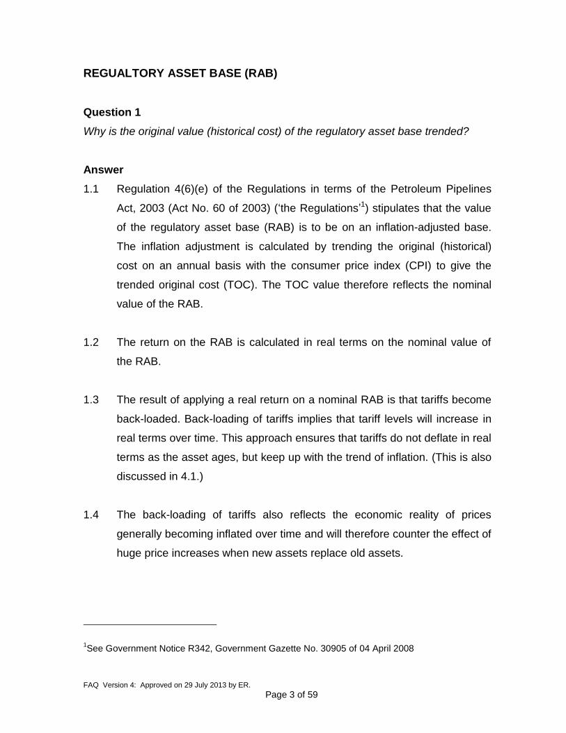
Note:
Further clarity on the meaning of non-current assets allowable in the RAB can be
obtained from the Regulatory Reporting Manual, Volume 4, which gives the following
classifications:
ASSETS AND OTHER DEBITS
Current Assets
100 Cash and Cash Equivalents
110 Accounts Receivable
110.003 Accounts Receivable – Trade
110.004 Accounts Receivable – Other
115 Accumulated Provision for Doubtful Debts
120 Inventory
120.001 Materials and Operating Supplies
120.003 Petroleum Inventory
125 Prepayments
135 Other Current Assets
Deferred Debits
142 Preliminary Surveys and Investigation Charges
147 Other Deferred Debits
Non-Current Assets
171.001 Plant in Service
171.002 Accumulated Depreciation – Plant in Service
172.001 Plant under capital leases and Improvements to leased facilities
172.002 Accumulated Depreciation – Leased Plant and Improvements
176 Line Fill
195.002 Other Intangible Assets

FAQ Version 4: Approved on 29 July 2013 by ER.
Page 7 of 59
LIABILITIES AND OTHER CREDITS
Current Liabilities
200 Bank Overdraft
205 Accounts Payable
206 Account Payable to Affiliated Companies
212 Obligations under Capital Leases – Current Portion
216 Interest Payable and Accrued
220 Dividends Payable
230 Accrued Income Taxes Payable
235 Other Current Liabilities
Deferred Credits
238 Unamortized Debt Premium and Expenses
241 Other deferred credits
Non-Current Liabilities
245 Provision for Pension and Benefits
255 Long-Term Debt
256 Long-Term Debt-Advances from Affiliated Companies
265 Other Non-Current Liabilities
265.001 Obligations under capital lease – non-current
265.002 Accumulated provision for self insurance
Owners’ Equity
275 Equity Issued
275.001 Ordinary shares issued
275.002 Preference shares issued
280 Contributed Surplus
285 Reserves including excess of appraisal value over depreciated plant
cost
290 Retained Earnings

FAQ Version 4: Approved on 29 July 2013 by ER.
Page 8 of 59
Question 2
Why is the Trended Original Cost not applied to the working capital component of the
RAB-formula?
Answer
2.1 Working capital resets itself each year and therefore there is an automatic
annual adjustment for inflation in the components of working capital.
2.2 If a multi-year tariff application is submitted, the working capital (W) should
be inflated with the CPI as at 12 months prior to the specific tariff period.
Question 3
What benchmarks are used for determining the allowable amounts for the respective
elements in the formula for determining the working capital?
Net working capital = inventory + linefill + receivables +
operating cash – trade payables
Answer
3.1 Inventory: Inventory is to be valued at the lower of cost or net realisable
value.
3.2 Llinefill: Linefill is to be valued at cost of product.
3.3 Receivables: Receivables is to be based on a maximum of 30 days of a
licensee’s allowable revenue.
3.4 Operating cash: Operating cash is to be based on a licensee’s standard
practice subject to a maximum of 45 days’ maintenance and operating
expenses, excluding depreciation and deferred taxes. Added to this amount
will be the minimum cash requirements of a licensee’s lender(s).

FAQ Version 4: Approved on 29 July 2013 by ER.
Page 9 of 59
3.5 Trade payables: Trade payables is to be based on a maximum of 45 days
of a licensee’s allowable revenue.
3.6 If licensees have proof that their actual values for the above benchmarks
are higher, the higher values can be used.
Question 4
Why is a deferred tax liability deducted and a deferred tax asset added to the RAB in
the RAB formula?
Answer
4.1 A deferred tax liability represents a temporary return of capital on which no
return is allowed and therefore it is deducted from the RAB. As the licensee
starts repaying the deferred taxation to the Receiver of Revenue, the
deduction from the RAB reduces.
4.2 A deferred tax asset represents additional capital investment. The NERSA
tax formula (paragraph 4.5 of the Tariff Methodology for the setting of tariffs
in the petroleum pipelines industry – hereinafter ‘the Methodology’)
assumes the cash 'to be received' from the fiscus, but the actual cash flow
benefit from the fiscus materialises only in later years and therefore a return
would be allowed on this investment. Deferred tax assets arise mostly as a
result of assessed taxation losses not utilised and carried forward.
4.3 The deferred taxation liabilities and assets are not trended.
WACC – GENERAL
Question 5
Why is a real WACC and not a nominal WACC applied?

FAQ Version 4: Approved on 29 July 2013 by ER.
Page 10 of 59
Answer
5.1 As explained under question 1, Regulation 4(6)(e) stipulates that the value of
the RAB has to reflect an inflation-adjusted value. Because the nominal value
of the RAB is used, a real rate of return is used [as reflected in the real
weighted average cost of capital (WACC)]. This requirement is also stipulated
in section 28(3)(c) of the Petroleum Pipelines Act, 2003 (Act No. 60 of 2003).
5.2 Inflation is added to the asset base (RAB) and is therefore 'taken out' of the
nominal return (WACC). Nominal returns on real assets would constitute a
double count of CPI and thus 'real returns' are used.
Question 6
What is to be understood by the following two statements?
i) Section 28(3)(c) of the Petroleum Pipelines Act 2003 (Act No. 60 of 2003) (the
Act):
(3) The tariffs set or approved by the Authority must enable the licensee to-
(c) make a profit commensurate with the risk;
ii) Section 4(6) of the Regulations made in terms of the Petroleum Pipelines Act
(see Government Notice R432, Government Gazette No. 30905 of 04 April
2008):
(6) The allowed revenue to be derived from tariffs contemplated in sub-
regulation (2) must include:
a) reasonable operating expenses
b) reasonable maintenance expenses
c) depreciation expenses
d) reasonable working capital
e) reasonable real return on the regulatory asset base which should
be determined on the assets’ inflation-adjusted cost less
accumulated depreciation; and
f) other applicable obligations.

FAQ Version 4: Approved on 29 July 2013 by ER.
Page 11 of 59
Answer
6.1 The reasonable return relates to the return earned by the licensee on the RAB
and not to the return earned by an equity investor on the RAB. Note that Sub-
regulation (2) refers to an ‘efficient licensee’ and not an equity holder as an
entity different from the licensee.
6.2 In view of the fact that Section 28(3) of the Act does not stipulate that the ‘profit
commensurate with risk’ is to be earned in each year, it is taken that the ‘profit’
(return) is to be earned over the total life of the asset. This profit relates to the
profit of the licensee on the RAB and not to the profit of an equity investor as a
separate construct.
6.3 The actual return that will be earned by the equity investor each year is a
function of the capital structure of the licensee. If the funding structure of the
licensee requires the debt funding to be repaid earlier or faster than the life of
the asset, it is viewed that the equity holder has chosen to become a 'patient
capital' investor. The ‘patient capital’ investor will therefore wait for the debt
capital to be repaid before the full return on equity can be earned.
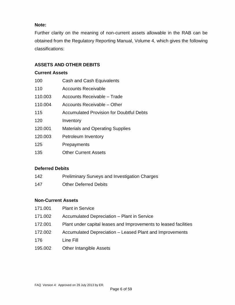
6.4 Figures 1, 2, 3 and 4 demonstrate the effect on the annual returns on equity
(ROE) under the following two scenarios (patient capital investor):
a) debt tenure of 10 years; and
b) debt tenure of 25 years.
FAQ Version 4: Approved on 29 July 2013 by ER.
Page 12 of 59
Figure 1: ROE per annum (debt = 10 years with equity earned over a period of 10 years)
Figure 2: ROE per annum (debt = 10 years with equity earned over a period of 25 years)
ROE per annum (10 years debt)
0.0%
5.0%
10.0%
15.0%
20.0%
25.0%
1 2 3 4 5 6 7 8 9 10 11
Years
RO
E %
Notional TAX with Deferred Tax adjusted to RAB Required ROE Flow-through actual tax
ROE per annum (10 year debt)
0%
10%
20%
30%
40%
50%
60%
70%
80%
90%
100%
1 2 3 4 5 6 7 8 9 10 11 12 13 14 15 16 17 18 19 20 21 22 23 24 25
Years
RO
E %
Notional TAX with Deferred Tax adjusted to RAB Flow-through actual tax Required ROE
FAQ Version 4: Approved on 29 July 2013 by ER.
Page 13 of 59
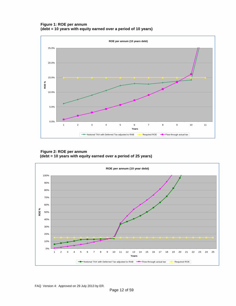
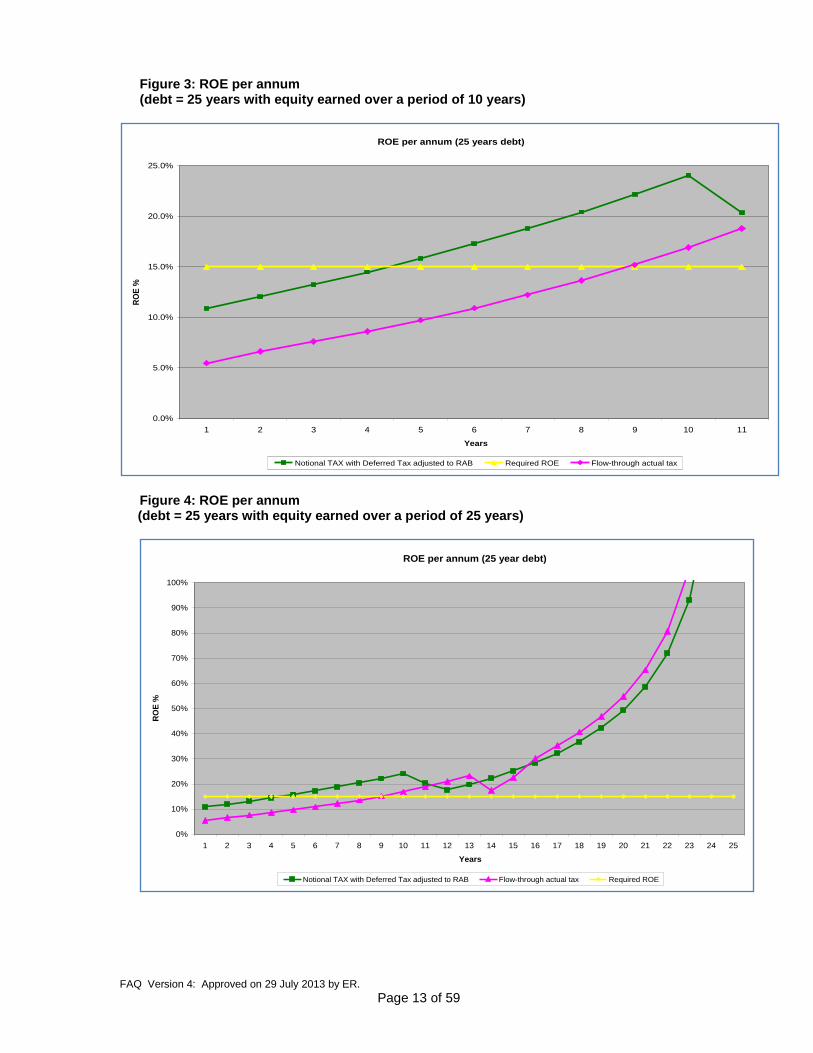
Figure 3: ROE per annum (debt = 25 years with equity earned over a period of 10 years)
Figure 4: ROE per annum (debt = 25 years with equity earned over a period of 25 years)
ROE per annum (25 years debt)
0.0%
5.0%
10.0%
15.0%
20.0%
25.0%
1 2 3 4 5 6 7 8 9 10 11
Years
RO
E %
Notional TAX with Deferred Tax adjusted to RAB Required ROE Flow-through actual tax
ROE per annum (25 year debt)
0%
10%
20%
30%
40%
50%
60%
70%
80%
90%
100%
1 2 3 4 5 6 7 8 9 10 11 12 13 14 15 16 17 18 19 20 21 22 23 24 25
Years
RO
E %
Notional TAX with Deferred Tax adjusted to RAB Flow-through actual tax Required ROE
FAQ Version 4: Approved on 29 July 2013 by ER.
Page 14 of 59
Note
1. Once the debt has been paid off, the equity starts ‘catching up’ (around years
six to eight) and the actual return to equity is at higher levels. The higher
levels of equity returns reflect the ‘catching up’ of returns that should have
been earned in previous years, but were forfeited because of having to pay
off debt (‘patient capital’).
2. The conversion of the RAB to a nominal value (TOC) and the subsequent real
WACC that is to be earned on the nominal value result in the ‘addition’ of CPI
values to the asset base that do not match the ‘reduction’ of the value of the
return in earlier years, because the return is calculated in real terms. The
returns in earlier years are lower as it takes time for the TOC effect to catch
up with the real return effect. Over the life of the asset, the return equalises
out.
3. Note that a minimum debt to total capital level of 30 per cent is assumed as
per paragraph 5.1.4 of the Methodology.
WACC – BETA
Question 7
Why is a beta derived from international companies used in relation to the conditions
of the local market?
Answer
7.1 There are no suitable comparative companies listed on the local markets.
Question 8
What are the criteria for selecting the betas of specific companies as a proxy for local
companies?

FAQ Version 4: Approved on 29 July 2013 by ER.
Page 15 of 59
Answer
8.1 The proxy companies must be listed on stock exchanges.
Question 9
Does NERSA publish beta values?
Answer
9.1 Yes, NERSA publishes the value of the unlevered beta applicable to the
petroleum industry. The names of the proxy companies utilised for determining
the beta value as well as quarterly updates on monthly beta values are
published on NERSA’s website.
Question 10
When are adjustments to the industry beta allowed?
Answer
10.1 No adjustments to the beta are allowed. The beta is a measure of systematic
risk. Company or project-specific risks should be accounted for separately from
the beta as explained in the tariff methodology.
Question 11
Which company is used as a supplier of data on beta values of proxy companies?
Answer
11.1 Data is collected monthly on the beta values of proxy companies and is based
on data provided by Bloomberg.
Question 12
At what frequency and over which period is data on the beta value of proxy companies
collected?

FAQ Version 4: Approved on 29 July 2013 by ER.
Page 16 of 59
Answer
12.1 Monthly data for a period of five years is collected. The five-year period is the
period ending the year immediately preceding the date of publication, which is
at the end of March of every year.
Question 13
Is a statistical correction factor applied to the values of the beta?
Answer
13.1 NERSA does not apply any additional correction factor to data utilised for
calculating the beta.
Question 14
How is the beta calculated?
Answer
14.1 The following example demonstrates how the beta (β) is calculated.
For licensees that are not publicly listed and where there are insufficient
publicly listed competitors, the equity beta is derived from a proxy beta. To
make adjustments for differences in gearing between the proxy and the
licensee the process involves ‘un-levering’ and ‘re-levering’ as follows:
i. obtaining the equity beta for the proxy company;
ii. un-levering the beta of the proxy company by the gearing level of the
proxy company – this unlevered beta is known as the asset beta;
iii. calculating the weighted average of the asset betas for the chosen
proxy companies; and
iv. re-levering the average asset beta by the (approved) gearing of the
licensee.

FAQ Version 4: Approved on 29 July 2013 by ER.
Page 17 of 59
14.2 Further clarification
i. The Harris and Pringle formula, which excludes the tax shields in the
notation, will be used.
ii. The following steps must be followed when calculating the beta value:
Step 1 – Calculate asset beta (or un-levered beta) for proxy firms
The following formula must be used to determine the asset beta:
β a1 = β1 / [1 + Dt/Eq]
Where:
βa1 = Asset beta for proxy company 1
β1 = Beta of proxy company 1
Dt = Debt of proxy company 1
Eq = Equity of proxy company 1
Repeat Step 1 for each of the six (or more) chosen proxy firms.
Market values for proxy companies will be used where such
market values exists. Where no market values exist for proxy
companies, book values will be used.
Step 2 – Calculate weighted average asset beta of proxy firms
Weight each of the 6 (or more) proxy firm asset betas by their
proportion of the total debt plus equity of the 6 (or more) proxy firms
and sum the results using the following formula:
n
n
1nna
n
1nn
na )(*
EqDt
EqDtE
Where:
βaE = Weighted average asset beta of the proxy companies
nEqDt = Sum of the debt and equity for a specific proxy
company

FAQ Version 4: Approved on 29 July 2013 by ER.
Page 18 of 59
na = Asset beta of the corresponding specific proxy
company
nn
1nEqDt
= Sum of debt and equity for all proxy companies
n = Number of proxy companies
Step 3 – Calculation of beta (β) for licensee (re-levering of beta)
The following formula must be used to determine the beta for the
licensee:
BL = βaE * [1 + Dt/Eq]
Where:
ΒL = Beta for the licensee
βaE = The weighted average β of the proxy firms asset betas
from Step 2. The Energy Regulator may adjust this
factor to take account of a difference in country risk
ratings between the host country of the proxy firms and
South Africa.
Dt = The interest bearing debt of the licensee subject to a
minimum gearing level of 30 per cent
Eq = The equity of the licensee
WACC – THE MARKET RETURN (MR)
Question 15
What market index will be used as a proxy for the performance of the South African
market?
Answer
15.1 The All Share Total Return Index (ALSI) is used as a proxy for the performance
of the South African market as it represents the widest possible spectrum of

FAQ Version 4: Approved on 29 July 2013 by ER.
Page 19 of 59
industries trading in the South African market, as measured by the
Johannesburg Stock Exchange (JSE).
Question 16
Why is a post-tax market return (MR) used for determining the market risk premium
(MRP)?
Answer
16.1 The market returns, as represented by the various JSE indices, reflect earnings
after taxation has been provided for (i.e. data is presented on an after-tax
basis).
16.2 No adjustment for Capital Gains tax is made as it is assumed that the equity
return holders will hold the investment to maturity and therefore the total return
index (TRI) is used.
16.3 There are flaws and challenges inherent in using the ‘post-tax’ MR as a basis
and converting it to a ‘pre-tax’ MR by grossing it up with the tax rate. This
method is thus not used by NERSA.
16.4 As the Allowable Revenue formula treats Taxation as a separate ‘operational’
item (T), the WACC calculations are all performed on a post-tax basis.
WACC – THE RISKFREE RATE (RF)
Question 17
Why are government bonds with a maturity of ten years or longer used?
Answer
17.1 An investor in pipeline infrastructure normally has a long-term investment
horizon of at least ten years. A maturity of less than ten years is considered to

FAQ Version 4: Approved on 29 July 2013 by ER.
Page 20 of 59
be subject to short-term fluctuations in the economic environment which could
impact on the volatility and validity of this measure for the industry.
17.2 Longer term investment instruments are also more in line with the 25-year MR
data used in calculating the WACC.
Question 18
What data sources does NERSA use and how frequently does NERSA publish
economic data for the purpose of tariff setting and approval?
Answer
18.1 The sources of the economic data utilised by NERSA and the frequency of
updating the economic data are provided in Table 2 below.
Table 2: Economic data sources and frequency of updates as provided by
NERSA for tariff setting and approval in the petroleum industry
Data Source Date & frequency of updating the
data on NERSA’s website
CPI-Historical
Statistics SA
Quarterly updates of monthly data
RSA 10-year Bonds
Reserve Bank of SA
Quarterly updates of monthly data
Market Return
ALL Share Total Return Index
(ALSI-TRI) on the JSE
Quarterly updates of monthly data
List of Beta proxy
companies as well as the
value of the beta applicable
for the tariff period
Quarterly updates of monthly data

FAQ Version 4: Approved on 29 July 2013 by ER.
Page 21 of 59
WACC – COST OF EQUITY (KE)
Question 19
Are any adjustments to the cost of equity allowed?
Answer
19.1 The following adjustments to the Cost of Equity (Ke) will be considered on a
case-by-case basis:
CRA = Country risk adjustment.
(The real CRA will be added to the riskfree rate. The CRA is
for assets in another country outside South Africa that are an
integral part of the same asset/s within South Africa. The
adjustment is for the other country concerned)
SSP = Small stock premium. An adjustment to compensate for the
lack of specific qualitative abilities of a licensee if warranted
α = Project specific risk if the circumstances warrant such an
adjustment
LP = Liquidity premium to accommodate assets which are not
publicly traded if the circumstances warrant such an
adjustment.
Note
A small stock premium and project specific risk adjustment
will be considered in the following cases:
a) SSP adjustments:
If the answers to the following two questions are ‘No’,
then a SSP adjustment may be applied:
In running its business:
i. does the licensee have access to legal, financial and
operational/technical expertise within its own

FAQ Version 4: Approved on 29 July 2013 by ER.
Page 22 of 59
structures/or can the licensee obtain this expertise
from its shareholders; and
ii. is there a history of the licensee having had access to
this expertise under its a previous shareholding
dispensation?
b) Project specific risk adjustments (if the circumstances
warrant such an adjustment)
The Energy Regulator needs to be provided with proof of
the following project specific risk factors:
- construction;
- management;
- technology;
- customer base;
- supplier chain; and
- other.
Question 20
How is the cost of equity calculated?
Answer
20.1 A practical example for calculating the Ke is presented below, making use of
assumed values for the respective elements in the formula for calculating Ke.
The formula for determining the Ke is:
Ke = Rf + (β *MRP)
Where:
Ke = Post-tax, real cost of equity
FAQ Version 4: Approved on 29 July 2013 by ER.
Page 23 of 59
Rf = Riskfree rate of interest (real).
(This is the average of the real monthly marked-to-market
riskfree rate for the preceding 300 months for all Government
bonds with at least a 10 year maturity as at 12 months before
the commencement of the tariff period under review)
β = ‘Beta’ is the systematic risk parameter for regulated entities
providing pipeline, storage and loading facility services
(The beta must be determined by proxy. As a proxy the
average of at least six pipeline companies listed on stock
exchanges is used. The value of the proxy is as at 12 months
before the commencement of the tariff period under review).
MRP = Market risk premium (post-tax, real).
[The proxy used for the market is the Johannesburg Stock
Exchange (JSE) All Share Total Return Index (ALSI with JSE
Code J203T) for the preceding 300 months as at 12 months
before the commencement of the tariff period under review.
The arithmetic average for the 300 months is used.]
Note
Two scenarios are considered – the first where the cost of equity is adjusted for
liquidity by multiplying a factor, and the second where the cost of equity is
adjusted for liquidity by adding a factor. Examples to calculate these are
presented next.
Multiplying to adjust for liquidity:
In the practical example for calculating the Ke (and multiplying to adjust for
liquidity), the values for the elements in the Ke formula are assumed to be as
follows:
Rf = 4.5%
CRA = 0.2%
MRP = 7%
β = 0.5

FAQ Version 4: Approved on 29 July 2013 by ER.
Page 24 of 59
SSP = 2.25%
α = 0.10%
LP = 5%
Based on the above assumed values, the value of the Ke is calculated to be:
Ke = [(Rf + CRA) + (MRP * beta) + SSP + α] * (1 + LP)
= [(4.5% + 0.2%) + (7% * 0.5) + 2.25% + 0.10 %] *(1 + 5%)
= (4.7% + 3.5% + 2.25% + 0.10%) *1.05%
= 11.08%
Adding to adjust for liquidity:
In the practical example for calculating the Ke (and adjust for liquidity through
adding), the values for the elements in the Ke formula are assumed to be as
follows:
Rf = 4.5%
CRA = 0.2%
MRP = 7%
β = 0.5
SSP = 2.25%
α = 0.10%
LP = 0.53%
Based on the above assumed values, the value of the Ke is calculated to be:
Ke = (Rf + CRA) + (MRP * beta) + SSP + α + LP
= (4.5% + 0.2%) + (7% * 0.5) + 2.25% + 0.10 % + 0.53%
= 4.7% + 3.5% + 2.25% + 0.10% + 0.53%
= 11.08%
FAQ Version 4: Approved on 29 July 2013 by ER.
Page 25 of 59
WACC – COST OF DEBT (Kd)
Question 21
Why is the real cost of debt (Kd) used and not the nominal cost of debt?
Answer
21.1 The inflation adjustment in the cost of debt (Kd) is ‘taken out’ as this is
‘replaced’ with the trending of the full value (PPE-d) of the original cost to give
the nominal TOC of the RAB.
21.2 Nominal returns on real assets would constitute a double count of CPI and
therefore ‘real returns’ are used.
Question 22
Under what scenario will equity investors be in a position to earn their full return as
embedded in the Ke portion of the WACC?
Answer
22.1 The reasonable return relates to the return on the asset for the licensee and not
for the equity investors. The actual return that will be earned by the equity
investor is a function of the capital structure of the licensee as was explained
under question 5. If the funding structures of the licensee require the debt
funding to be repaid earlier or faster, it is viewed that the equity holder has
chosen to become a ‘patient capital’ investor. The ‘patient capital’ investor will
wait for the debt capital to be repaid before they receive their required return.
22.2 The conversion of the asset base (PPE-d) to a nominal value (TOC) and the
subsequent conversion of WACC into real WACC results in the ‘addition’ of CPI
to the asset that does not ‘match’ the ‘reduction’ of the rate in earlier years.
Therefore, the returns in earlier years are lower as it takes time for the TOC
effect to catch up with the real return effect. Once the catch up has taken place

FAQ Version 4: Approved on 29 July 2013 by ER.
Page 26 of 59
(around years 6 to 8), the return will be superior. (See graphs in question 4
above.)
Question 23
Does the post-tax, real WACC not allow the entity enough allowable revenue to pay
back its debt which is payable in pre-tax nominal terms? [The WACC (Ke & Kd) is
provided for only on a post tax, real basis.]
Answer
23.1 No. The tax shield in the Kd is provided for in the tax formula where the post-tax
Kd is grossed up with the tax shield portion of the Kd. This ensures a pre-tax Kd
is provided for in the allowable return to match the payment of the financing
costs in nominal values. (See formula in paragraph 7.3 of Methodology.)
23.2 In tables 3 and 4 below, the calculation of tax (as per the tax formula in the tariff
Methodology) is demonstrated. For each component which is taxable, a gross-
up at the existing tax rate is performed. Tax allowances are therefore provided
for in these grossed-up balances and will be included in the total balance of the
allowable revenue.
23.3 As can be seen from tables 3 and 4, the grossing up of balances also applies to
the Kd to ensure the tax shield on the Kd is properly accounted and provided
for.

FAQ Version 4: Approved on 29 July 2013 by ER.
Page 27 of 59
Table 3: Treatment of WACC with Notional Tax
Allowable Revenue = (RAB x WACC) + E + T + D + F ± C.
RAB WACC E D (historic) D
(amortisation of write-up)
T taxation) Total
allowable revenue
WACC = [Rf + (MRP*beta)*Ke] + [Kd*debt] Ke Kd WACC
Gearing 51% 49%
NERSA decision (returns %) 9.52% 3.47% 6.56%
NERSA decision value (R million) 105.00 5.10 1.78 6.88 3.00 4.00 0.20 14.08
NRBTA = {(RAB*WACC) + D + E + F ±C} - {E + D(historic)}.
0.00 0.00 0.00 (3.00) (4.00) (7.00)
NRBTA 5.10 1.78 6.88 0.00 0.00 0.20 0.00 7.08
Taxation (gross up and notional tax) 1.98 0.69 2.68 0.00 0.00 0.08 2.75 2.75
Add back tax deductions 0.00 0.00 0.00 3.00 4.00 0.00 0.00 7.00
Total revenue including notional tax 7.08 2.48 9.56 3.00 4.00 0.28 2.75 16.84
All these WACC components are not deducted to arrive at a taxable income before tax allowance. They first become grossed up. By grossing up and then adding a notional tax allowance, they all effectively become pre-tax. The applicant therefore receives the tax which he is going to pay to the fiscus.
These components are tax deductible and there-fore do not need a tax shield.
The argument sometimes is that the amortisation of the write-up (effectively to counter for the "loss" of CPI in the conversion of nominal rates to real rates) is affecting the after-tax returns. This component is also awarded a tax shield in the calculation and the applicant receives the tax allowance it needs to pay the fiscus. There is obviously a time delay.

FAQ Version 4: Approved on 29 July 2013 by ER.
Page 28 of 59
Table 4: Treatment of WACC with flow-through tax
Allowable Revenue = (RAB x WACC) + E + T + D + F + C
RAB WACC E D & wear &
tear (historic)
D (amortisation of write-up)
T(taxation) Total
allowable revenue
WACC=[Rf+(MRP*beta)*Ke]+[Kd*debt] Ke Kd WACC
Gearing 51% 49%
Returns % 9.52% 3.47% 6.56%
Returns (R million)
105.00 5.10 1.78 6.88 3.00 4.00 0.20 14.08
NRBTA ={(RAB*WACC)+D(historic & write-up)+ E+F+-C}-{E+wear & tear allowance(historic) +Kd(nominal)} 0.00 (5.88) 0.00 (3.00) (10.00) (13.00)
NPBT excl tax allowance 5.10 (4.10) 6.88 0.00 (6.00) 0.20 0.00 1.08
Taxation (gross-up and notional tax) 1.98 (1.59) 0.39 0.00 (2.33) 0.08 (1.87) (1.87)
Add back tax deductions 0.00 5.88 0.00 3.00 10.00 0.00 0.00 13.00
Total revenue including flow- through tax with tax shield on Kd
7.08 0.19 7.27 3.00 1.67 0.28 (1.87) 12.22
All these WACC components (except Kd) are not deducted to arrive at a taxable income before tax
allowance. By grossing up and then adding a notional tax allowance, they all effectively
become pre-tax. The applicant therefore receives the tax which he is going to pay. Tax shield on
Kd not given.
These components are tax deductable and therefore do not need a tax shield.
The argument is sometimes that the amortisation of the write-up (effectively to counter for the "loss" of CPI in the conversion of nominal rates to real rates) is affecting the after-tax returns. This component is also awarded a tax shield in the calculation.
FAQ Version 4: Approved on 29 July 2013 by ER.
Page 29 of 59
Question 24
Why is Vanilla WACCreal (pre-tax Kd and post-tax Ke) not used instead of grossing up
the post-tax Kd to ensure that the tax shield of the Kd is provided for in the before tax
allowable revenue?
Answer
24.1 Vanilla WACC is a calculation where the Ke is post-tax and the Kd is pre-tax.
24.2 The taxation component for the cost of debt is ‘given’ to the investor by allowing
the ‘tax shield’ in the calculation of taxation allowance (T) as is demonstrated in
the above Table 3 and Table 4.
24.3 The Vanilla WACCreal results in a higher return relative to the notional or flow-
through (with tax shield) options and therefore it is not utilised by NERSA. This is
demonstrated in the published model in the TAB ‘flow-through Vanilla’ where the
return achieved is 15.5 per cent, which is higher than the 15 per cent required
return.
DEPRECIATION
Question 25
How is depreciation and amortisation of the write-up portion calculated?
Answer
25.1 See example in Table 1 of Question 1.

FAQ Version 4: Approved on 29 July 2013 by ER.
Page 30 of 59
EXPENSES – LAND REHABILITATION
Question 26
What is the legal and regulatory foundation for the recovery of land rehabilitation cost?
Answer
26.1 In terms of the Petroleum Pipelines Act, 2003 (Act No. 60 of 2003) the authority
may require a licensee to submit a financial security, or make such other
arrangements as may be acceptable to the Authority, to ensure compliance with
any licence condition relating to health, safety, security, or the environment, prior
to, during or after the period of validity of the licence. Regulation 9 (4) of the
regulations in terms of the Petroleum Pipelines Act, 2003 (Act No. 60 of 2003)
provides that the authority must require the licensee to provide financial security
for the purpose of rehabilitating land used in connection with a licensed activity
and the composition and amount of such security. Paragraph 6.4.7 of the
Methodology states ‘Provision for land rehabilitation costs are permitted, subject
to adequate justification. These funds must be kept in accordance with the
Petroleum Pipelines Act, 2003 (Act No. 60 of 2003) and sub-regulation 9 of
Regulations made in terms of the Act published under GN R342 in Government
Gazette 30905 of 4 April 2008’.
26.2 Paragraph 6.2 and 6.3 of the methodology refers to the classification and
calculation of the operating expenses (inclusive of the land rehabilitation costs as
per paragraph 6.4.7)
26.3 Sub-regulation 9 states:
(1) Licensees must, not less than six months prior to termination,
relinquishment or abandonment of licensed activities, submit to the
Authority a plan for approval for the closure, removal and disposal, as the
case may be, of all installations relating to such licensed activities.
(2) The plan contemplated in sub-regulation (1) must include information

FAQ Version 4: Approved on 29 July 2013 by ER.
Page 31 of 59
regarding—
(a) alternatives investigated for further use and alternative disposal of
the installations;
(b) decommissioning activities;
(c) site cleanup, removal and disposal of dangerous material and
chemicals; and
(d) an environmental impact assessment of the termination and
abandonment of the licensed activity concerned.
(3) The Authority may approve the plan contemplated in sub-regulation (1)
subject to any condition or amendment that the Authority may determine.
(4) The Authority must require the licensee to provide financial security for
purposes of rehabilitating land used in connection with a licensed activity
and the composition and amount of such security.
(5) Financial security contemplated in sub-regulation (4) may be in any form
acceptable to the Authority and may only be used with the approval of
the Authority.
(6) The Authority may, in writing, at any time, require written confirmation
from a licensee that it is in compliance with the requirements of the
National Environmental Management Act, 1998 (Act No. 107 of 1998).
(7) The Authority may require written proof from the licensee that the
authority responsible for administering the Act referred to in sub-
regulation (6) has approved the environmental impact assessment
required by the Act in question.
(8) The Authority may not, before it is in receipt of a certificate from an
independent consultant competent to conduct environmental impact
assessments in accordance with the provisions of the National
Environmental Management Act, 1998 (Act No. 107 of 1998), stating that
the site has been rehabilitated, give consent to the termination of a
financial security arrangement contemplated in sub-regulations (4) and
(5).

FAQ Version 4: Approved on 29 July 2013 by ER.
Page 32 of 59
26.4 The financial instrument must be in a form acceptable to the Energy Regulator as
required by section 9 (5) of the regulations. To ensure compliance in this regard it
would be the most practical for the financial security structure to be approved by
the Energy Regulator in advance. The guidelines the Energy Regulator would
apply when evaluating the financial security as referred to in regulation 9 (4) and
(5) are:
- a secure financial instrument with the objective of beating inflation; and
- a legal framework to ensure that such funds cannot be accessed by
normal operational funding needs or creditors. This would probably
require some sort of Trust structure.
Question 27
How should land rehabilitation costs be calculated and recovered trough the Allowable
Revenue?
Answer
27.1 Land rehabilitation costs are recovered as part of operating expenses.
27.2 Land rehabilitation cost can therefore NOT be included as part of Property, Plant
and Equipment (RAB) and therefore no return is earned thereon.
27.3 The mechanism to collect the land rehabilitation costs is the present value of the
future liability less the value of funds in the ‘decommissioning fund’ to arrive at a
balance still to be collected. The remaining balance is then divided by the
remaining years to decommission the asset. The formula for this is:
PMT=[PVfund value]/n
Where
N = the number of remaining years to decommission
PVfund value = the present value of decommissioning costs

FAQ Version 4: Approved on 29 July 2013 by ER.
Page 33 of 59
Fund value = the current balance in the decommissioning fund, being historic
contributions (provision for decommissioning costs) plus net
returns on such contributions.
27.4 An example of how the land rehabilitation cost is to be calculated is presented in
Table 5.

FAQ Version 4: Approved on 29 July 2013 by ER.
Page 34 of 59
Table 5: An example on the calculation of land rehabilitation costs
Asset value
10,00
0 PV of expected
rehabilitation cost
6,000
Life of Asset
10yrs
1 2 3 4 5 6 7 8 9 10
CPI a 5% 6% 4% 4% 6% 7% 8% 5% 4% 5% Net returns [after tax] in the fund b 6% 7% 5% 4% 6% 7% 8% 4% 4% 5%
Remaining Life c 10 9 8 7 6 5 4 3 2 1
Present value of Land rehabilitation liability
d=opening* (1+a)
6,000
6,360
6,614
6,879
7,292 7,802
8,426
8,848 9,202 9,662
Fund value at beginning of the year e= 0 (618) (1,317) (2,061) (2,846) (3,780) (4,877) (6,190) (7,341) (8,584)
Still to be recovered over remaining life f=d+e
6,000
5,742
5,297
4,817
4,446 4,022
3,549
2,658 1,860 1,078
To be recovered "this" year g=f/c
600
638
662
688
741 804
887
886 930 1,078
Value of fund
Opening Balance h=j
-
618
1,317
2,061
2,846 3,780
4,877
6,190 7,341 8,584 Contribution from allowable revenue via the tariff g
600
638
662
688
741 804
887
886 930 1,078
Net returns [after tax] in the fund i=(h+g*50%)*b
18
61
82
96
193 293
426
265 312
Closing Balance of fund j=h+g+i
618
1,317
2,061
2,846
3,780 4,877
6,190
7,341 8,584 9,662
Liability less Fund value k=d-j
5,382
5,043
4,553
4,033
3,512 2,925
2,236
1,506 618 -
Note
The value of the land rehabilitation liability in year 10 (R9,662) is covered by the value
of the fund at the end of that year (R9,662) excluding the investment returns in that
year.
27.5 For the above example, the Depreciation in the Allowable Revenue formula
compared to the allowance of the land rehabilitation on an annual basis is
demonstrated in Figure 5 below. Note that the upward trend is similar to achieving
the goal of raising tariffs as intended by the nominal assets, real return principle
used in the methodology.

FAQ Version 4: Approved on 29 July 2013 by ER.
Page 35 of 59
Figure 5: Depreciation and TOC Amortisation vs Land Rehabilitation cots
F-FACTOR
Question 28
How is the F-factor calculated and how will it be recovered?
Answer
28.1 Details are provided in Section 4.2.14 of the Tariff Methodology. The F-factor will
be treated as a return of capital, i.e. deducted from/added to the RAB.
CLAWBACK
Question 29
When will clawbacks be applied?
-
200
400
600
800
1 000
1 200
1 400
1 600
1 800
1 2 3 4 5 6 7 8 9 10
Depreciation and TOC amortization vs Land rehabilitation costs
Depreciation and TOC amortization Land rehabiliatation cost

FAQ Version 4: Approved on 29 July 2013 by ER.
Page 36 of 59
Answer
29.1 In the tariff period following the release of audited financial statements of the
applicant.
Question 30
Are there examples of specific clawback calculations?
Answer
30.1 The formula for clawback adjustments is as follows:
Clawback adjustments = ARA +(PPE-d)A + DA + KdA + EA + OeA + + + GA
Where:
ARA = Allowable revenue adjustment
(PPE-d)A = Allowable revenue adjustment on (PPE-d)updates
DA = Depreciation and amortisation of inflation write-up adjustment
KdA = Cost of debt adjustment
EA = Expenses adjustment
GA = General adjustment for any remaining differences between
projected allowable revenue and actual allowable revenue not
resulting from efficiency gains, for example:
i. debt ratio and the effect thereof on beta, cost of equity,
WACC and the taxation effect of these adjustments
ii. taxation adjustments
iii. other
OeA = Operating efficiency adjustment (Only if more efficient)
Note: Operating efficiency could result in clawbacks to or from a
licensee.
30.2 More detail on the formulas to determine clawbacks is presented below.

FAQ Version 4: Approved on 29 July 2013 by ER.
Page 37 of 59
30.2.1 Allowable Revenue adjustment (ARA)
The allowable revenue adjustment compensates the licensee and customers for
differences between allowable revenue planned and allowable revenue realised
in a specific tariff period. The following formula applies:
ARA = ARa - ARr
Where
ARA = Allowable revenue adjustment
ARa = Allowable revenue approved
ARr = Allowable revenue realised
30.2.2 Value of new operating property, plant and equipment adjustment (PPE-d)
The net value adjustment for operating property, plant and equipment (PPE-d)A
compensates licensees and customers for differences in operating assets
estimated to be in use and operating assets actually in use in the tariff period
under review. This pertains to changes arising from additions, decommissioning
and disposals of operating assets – as well as to the timing of implementing
these changes. Timing refers to the difference between the projected date and
the actual date when the changes were implemented.
Adjustments to the net value of the operating assets (PPE-d)A is determined by
applying the formula below:
(PPE-d)A = Allowable revenue adjustment on (PPE-d)updates
= [(PPE-d)updates x (Dya – Dyp)/365] x WACC
Where:
(PPE-d)updates = Net value of the operating assets that will be
commissioned, decommissioned or disposed of during the
tariff period under review.
Dya = Actual number of days from the date when the operating
asset(s) was commissioned, decommissioned or disposed of
to the end of the tariff period.

FAQ Version 4: Approved on 29 July 2013 by ER.
Page 38 of 59
Dyp = Projected number of days from the date when the operating
asset(s) was planned to be put into use, decommissioned
or disposed of to the end of the tariff period.
30.2.3 Depreciation and amortisation of inflation write-up adjustment (DA)
The depreciation and amortisation of inflation write-up adjustment provides for
the differences between the projected depreciation made at the time the
allowable revenue was determined and the actual depreciation for the specific
tariff period. The following formula must be applied:
DA = Da – Dp
Where:
DA = Depreciation and amortisation of inflation write-up adjustment
Da = Depreciation and amortisation of inflation write-up actual
Dp = Depreciation and amortisation of inflation write-up approved
30.2.4 Cost of Debt Adjustment (KdA)
If there is a difference between the estimated cost of debt in the allowable
revenue and the actual cost of debt for that tariff period, then the allowable
revenue must be recalculated using the actual cost of debt and the difference
added to or subtracted from the clawback adjustment. The following formula must
be used to determine the KdA:
KdA = Allowable Revenue recalculated using actual cost of debt –
Allowable Revenue calculated using approved cost of debt2
30.2.5 Expense adjustment – Operating and Maintenance Adjustment (EA)
Adjustments on operating and maintenance expenditure provides for differences
between expenditure projected at the time of setting the tariffs and the actual
2 All other factors and quantum in estimated Allowable Revenue remain the same.
FAQ Version 4: Approved on 29 July 2013 by ER.
Page 39 of 59
expenditure for the tariff period and is calculated by applying the following
formula:
EA = Ep – Ea
Where:
EA = Operating and maintenance expense adjustment
Ep = Operating and maintenance expense projected
Ea = Operating and maintenance expense actual
30.2.6 General adjustment (GA)
Provision is made for a general adjustment. This adjustment is for any
remaining differences between projected allowable revenue and actual
allowable revenue not resulting from efficiency gains, for example:
i. debt ratio and the effect thereof on beta, cost of equity, WACC and the
taxation effect of these adjustments;
ii. taxation adjustments; and
iii. other.
TAX
Choice between two different tax approaches
Question 31
What is the difference between flow-through tax and notional tax?
Answer
31.1 Section 10.2 of the Methodology states that the flow-through tax is the actual tax
paid by the entity and this is allowed as a tax allowance. Notional tax expense is
the tax due according to accounting requirements. Flow-through tax neither
awards the tax shield nor the benefits of accelerated wear and tear (or deferred
taxation).

FAQ Version 4: Approved on 29 July 2013 by ER.
Page 40 of 59
Question 32
How is the tax calculated under the following scenarios?
Flow-through tax
Notional tax
Answer
32.1 Examples on the calculation of tax under the two scenarios are provided in tables
6, 7, 8 and 9.
32.2 Calculation of the flow-through tax.
Tax = {(NRBTA) / (1-t)}*t
Where:
NRBTA = Net revenue before tax allowance
= {(RAB*WACC)+E+D(historic & write up)+F± C} -
{E+D(historic) +Kd(nominal)}.
t = prevailing corporate tax rate of the licensee

FAQ Version 4: Approved on 29 July 2013 by ER.
Page 41 of 59
Table 6: Example of the calculation of flow-through taxes
Ke a 5.10
Kd b 1.78
WACC c=a+b 6.88
E d 3.00
D (historic) e 4.00
D (write-up) ee 0.20
Wear and tear allowance eee 10.00
F f -
C [Claw back Excluding Tax claw back] g -
NRBTA=Allowable revenue before tax allowance h=c+d+e+ee+f+g 14.08
t j 28%
Kd (nominal) n 5.88
NRBTA={(RAB*WACC)+E+D(historic & write up)+F+-C}-{E+D(historic)
+Kd(nominal)} Note that interest is deducted as an actual tax
calculation is performed k=h-d-e-n (4.80)
Tax={(NRBTA excl tax allowance)/(1-t)}*t l={k/(1-j)}*j (1.87)
Total Allowable revenue m=h+l 12.22
Test tax rate l/(k+l) 28%
Note that no other non-taxable income or non-deductible expenses have been
included above. These will form part of the actual calculation when detail is
available.

FAQ Version 4: Approved on 29 July 2013 by ER.
Page 42 of 59
Table 7: The effect of using flow-through tax
Allowable Revenue = (RAB x WACC) + E + T + D + F + C
RAB WACC E D & wear and tear (historic)
D (amortisation of write-up)
T(taxation) Total
allowable revenue
WACC=[Rf+(MRP*beta)*Ke]+[Kd*debt] Ke Kd WACC
Gearing 51% 49%
Returns % 9.52% 3.47% 6.56%
Returns (R million)
105.00 5.10 1.78 6.88 3.00 4.00 0.20 14.08
NPBT excl tax allowance={(RAB*WACC)+E+D(historic & write-up)+F+-C}-{E+wear & tear allowance (historic) +Kd(nominal)} 0.00 (5.88) 0.00 (3.00) (10.00) (13.00)
NPBT excl tax allowance 5.10 (4.10) 6.88 0.00 (6.00) 0.20 0.00 1.08
Taxation (gross-up & notional tax) 1.98 (1.59) 0.39 0.00 (2.33) 0.08 (1.87) (1.87)
Add back tax deductions 0.00 5.88 0.00 3.00 10.00 0.00 0.00 13.00
Total revenue including flow-through tax with tax shield on Kd
7.08 0.19 7.27 3.00 1.67 0.28 (1.87) 12.22

FAQ Version 4: Approved on 29 July 2013 by ER.
Page 43 of 59
Table 8: Example on the calculation of notional tax
Tax = {(NRBTA) / (1-t)}*t Where NRBTA = Net revenue before tax allowance
= {(RAB*WACC) +E+D(historic & write-up) +F ± C} - {E+D(historic)}.
t = prevailing corporate tax rate of the licensee
Ke a
5.10
Kd b
1.78
WACC c=a+b
6.88
E d
3.00
D (historic) e
4.00
D (write-up) ee
0.20
Wear and tear allowance eee
10.00
F f -
C [Claw back Excluding Tax claw back] g -
NRBTA=Net revenue before tax allowance h=c+d+e+
ee+f+g
14.08
t j 28%
Kd (nominal) n
5.88
NRBTA={(RAB*WACC)+E+D(historic & write up)+F+-C}-{E+D (historic) } Note that interest is not deducted to allow for the tax shield on after tax real Kd. k=h-d-e 7.08
Tax={(NRBTA)/(1-t)}*t l={k/(1-
j)}*j 2.75
Total Allowable revenue m=h+l
16.83
Test tax rate l/(k+l) 28%

FAQ Version 4: Approved on 29 July 2013.
Page 44 of 59
Table 9: The impact of the ‘tax shield’ when notional tax is used
Allowable Revenue = (RAB x WACC) + E + T + D + F + C
RAB WACC E D
(historic)
D (amortisation of write-up)
T(taxation) Total
allowable revenue
WACC=[Rf+(MRP*beta)*Ke]+[Kd*debt] Ke Kd WACC
Gearing 51% 49%
Returns % 9.52% 3.47% 6.56%
Returns (R million)
105.00 5.10 1.78 6.88 3.00 4.00 0.20 14.08
NPBT excl tax allowance={(RAB*WACC)+E+D+F+-C}-{E+D(historic)}
0.00 0.00 0.00 (3.00) (4.00) (7.00)
NPBT excl tax allowance 5.10 1.78 6.88 0.00 0.00 0.20 0.00 7.08
Taxation (gross-up and notional tax) 1.98 0.69 2.68 0.00 0.00 0.08 2.75 2.75
Add back tax deductions 0.00 0.00 0.00 3.00 4.00 0.00 0.00 7.00
Total revenue including notional tax 7.08 2.48 9.56 3.00 4.00 0.28 2.75 16.84
Tax – deferred tax (dtax)
Question 33
Why is the deferred tax asset/liability not included in the RAB formula when the flow-
through tax option is chosen?
Answer
33.1 Deferred tax liabilities do not arise relative to the allowable revenue awarded
when the flow-through approach is taken because it is merely a timing issue of
when the tax will be paid and therefore it is not deducted in the RAB formula.
33.2 Deferred tax assets arising from tax losses in earlier years are not added in the
RAB formula to counteract the previous ‘competitive advantage’ enjoyed by the
entity because of this asset class.

FAQ Version 4: Approved on 29 July 2013 by ER.
Page 45 of 59
TARIFF MODEL ON NERSA’S WEBSITE
Question 34
Is there a practical example of how to incorporate all the elements of the tariff
methodology into one template?
Answer
34.1 NERSA has published a model on its website with the intention of
demonstrating the various options and scenarios by way of testing the target
cost of equity by the outcome of the internal rate of return (IRR) of cash flows to
investors.
34.2 Some general notes on the model as published on NERSA’s website are:
i. Base case – The model presents a base case scenario using the
notional tax option where no adjustments are made for deferred taxation
to the RAB.
ii. F-Factor – The model demonstrates the treatment of the F-factor as a
return of capital, i.e. the full value of the F-factor is deducted from/or
added to the RAB.
iii. Notional tax – This is the notional tax option with the deferred taxation
adjusted in RAB. Note that IRR is higher than targeted as the actual tax
and deferred tax cash flows practically lag one year.
iv. Tax formula notional – The model demonstrates the tax formula for
year 1 and also demonstrates the tax shield for each component of
allowable revenue.
v. Flow-through using Vanilla WACC – This represents a flow-through
option but with the Kd pre-tax. This means that the tax shield on the Kd
is not allowed in the tax calculation as the tax is already included in the
pre-tax rate. Also note that the ‘achieved IRR’ in this option is higher

FAQ Version 4: Approved on 29 July 2013 by ER.
Page 46 of 59
(15.50 per cent) than the targeted 15 per cent, which is why this option
is not followed.
vi. Flow-through actual – Flow-through tax is defined in the Methodology
(paragraph 10.2) as actual tax payments. As can be seen, the resultant
IRR is below the target IRR of 15 per cent, which is a result of the tax
shield on cost of debt not being allowed. For this reason, NERSA uses
the tax flow-through formula to calculate the tax allowance in the model.
vii. Graphs – The model also has ‘worksheet tabs’ comparing, by way of
data or graphs, the differences between the various tax options (flow-
through and notional tax) and tenures of debt (10 years versus 25
years).
NOTES ON MULTI-YEAR TARIFF APPLICATIONS
Question 35
How will NERSA treat multi-year tariff applications?
Answer
The treatment of multi-year tariffs is presented in the section that follows.
FAQ Version 4: Approved on 29 July 2013.
Page 47 of 59
Notes on multi-year tariffs in terms of the Petroleum Pipelines Act
Approved on 18 September 2012
1. Purpose
1.1 Regulating the tariffs charged for pipelines, storage and loading facilities within
the petroleum pipelines industry is a function of the National Energy Regulator
of South Africa (NERSA or ‘the Energy Regulator’). In doing so, NERSA applies
its tariff methodologies3. Throughout this paper, these methodologies are
referred to as ‘the Methodologies’. These Methodologies meet all the
requirements of the Petroleum Pipelines Act, 2003 (Act No. 60 of 2003) (‘the
Act’) and the Regulations in terms of this Act (‘the Regulations’).
1.2 Regulation 4(9)(a) of the Regulations provides licensees with the option to
follow a multi-year tariff dispensation when applying for tariff increases. Some
licensees have indicated that they intend to follow this approach and this
document serves to provide clarifying notes on implementing multi-year tariffs
within the petroleum pipelines industry.
3 Methodologies:
1. Tariff methodology for the setting of tariffs in the petroleum pipelines industry. 6th Edition.
Approved on 31 March 2011.
2. Tariff methodology for the approval of loading facilities and storage facilities. 2nd
Edition.
Approved on 31 March 2011.

FAQ Version 4: Approved on 29 July 2013 by ER.
Page 48 of 59
2. Summary
2.1 Tariffs are typically set for periods of one year, however in the case of multi-
year decisions, tariffs are set for a period of two to five years. Tariffs for the
years ahead are necessarily based on forecasts for various parameters. As a
general rule, the longer the forecast period is, the less accurate the forecasts
towards the end of the period are likely to be.
2.2 With the passing of time forecasts can be replaced with actual data for those
parameters. When sufficient actual data is available for a tariff year, the tariff
will be recalculated. If there is a difference, as is often the case, clawbacks or
give backs will be calculated. This will be done each year during a multi-year
tariff decision. Because actual data for tariff year one will only become available
in tariff year two, any clawback or giveback will only be implemented in tariff
year three
2.3 To lessen the impact of the uncertainty brought about with having to work with
estimated, forecasted and proxy values in a multi-year tariff determination, there
will be instances where NERSA will have to update such values with more
recent values. When the update needs to be done, it may require the opening of
the public participation process in order to amend the multi-year tariffs set or
approved. (See paragraph 6.2 for more detail.)
3. Definition of multi-year tariffs
3.1 The term ‘multi-year’ tariff determination means that tariffs for multiple
years/periods are being determined at one point in time.
FAQ Version 4: Approved on 29 July 2013 by ER.
Page 49 of 59
3.2 The Methodologies define a tariff period as a period of one year (12 months) –
which is the financial year of the licensee.
3.3 A multi-year tariff application implies that each of the components in the formula
for determining the allowable revenue (AR) for each of the years/periods will
have different values that need to be brought into consideration when setting
the allowable revenue for each of these years.
3.4 The adjustments to the values of the components are brought into account by
applying clawbacks (to and from the licensee). Guidance on how and when
these clawbacks will be done, as well as the terms and conditions for revising
the decision and therefore the re-opening of the public consultation process
pertaining to a specific multi-year tariff determination, are presented in the rest
of this document.
4. Components
The values of the components referred to above, are the values of specifically
identified components as contained in the following formulas:
4.1 Formula to calculate the allowable revenue (AR):
AR = (RAB x WACC) + D + E +F ± C + T
Where:
AR = Allowable revenue
WACC = Weighted average cost of capital
D = Depreciation and amortisation of inflation write-up for the tariff
period under review

FAQ Version 4: Approved on 29 July 2013 by ER.
Page 50 of 59
E = Expenses: actual and accrued operating and maintenance
expenses, including provisions for land rehabilitation costs, for
the tariff period under review
F = Projected revenue addition to meet debt obligations for the tariff
period under review
C = Clawback adjustments in all elements of clawback formula to
correct for differences between actuals and approved for a
preceding tariff period or periods.
T = Tax expense: estimated notional or flow through tax expense for
the tariff period under review
4.2 Formula pertaining to the composition of the RAB:
RAB = (PPE – d) + w ± dtax
Where:
PPE = Value of original and inflation write-up of operating assets
(property, plant and equipment)
d = Accumulated depreciation and accumulated amortisation of
inflation write-up for the period up to the commencement of the
tariff period under review
w = Net working capital
dtax = Deferred tax
4.3 Formula to calculate the weighted average cost of capital (WACC):
Kd*
EqDt
DtKe*
EqDt
Eq WACC
Where:
Eq = Shareholders equity
Dt = Interest bearing debt
Ke = Post-tax, real cost of equity derived from the capital asset pricing
model (CAPM)
Kd = Post-tax, real cost of debt

FAQ Version 4: Approved on 29 July 2013 by ER.
Page 51 of 59
4.4 Components in the formula to determine the cost of equity (Ke):
− Riskfree rate (Rf)*
− Market risk premium (MRP)* and
− Beta ( )*
Note:
The * indicates that as per these Methodologies, these values are to be
determined as at 12 months prior to the commencement of a specific tariff
year/period.
In a multi-year tariff determination, this means as at 12 months prior to the
commencement of each of the respective tariff years/periods. The application,
however, will reflect the value of these components only as at 12 months prior
to the first tariff year/period because only these are available.
4.5 Formula to determine the cost of debt(Kd):
1 - CPI 1
t)]-(1*[Kd1 Kd
nomtax,prenominaltax,-post
Where:
Kdpre-tax,nominal = Projected cost of debt, pre-tax, nominal, for the tariff period
under review
t = Prevailing corporate tax rate of the licensee.
CPI = Actual annual consumer price index (CPI) as at 12 months
prior to the commencement of the current tariff period under
review.
Note
This annual CPI is the same actual annual CPI included in the
calculation of the average used for converting year 25 in the
market risk premium (MRP) formula from its nominal to real
value.

FAQ Version 4: Approved on 29 July 2013 by ER.
Page 52 of 59
5. Categories of values
The values of the components can broadly be classified into the following three
categories:
5.1 Estimated Values
i. These are the estimated values of the components as at the time of
applying for the tariff determination. These values are then later updated
with the actual values. The differences between the estimated and actual
values for a particular year will be clawed back (to or from the licensee).
The clawback will be calculated once a particular tariff year/period has
expired and the actual values are available.
ii. The following components are included in this category:
- the regulated asset base [RAB];
- operational expenditure [E];
- depreciation [D];
- nominal cost of debt [Kdnom];
- debt ratio;
- tax rate [t]; and
- volumes shipped [Vol].
5.2 Proxy Values
i. The value of these components is 'proxies' based on actual data 12
months prior to the commencement of the tariff period. In a single year
tariff application, these values will always be known at the time of the
application and no adjustments need be made.
ii. In a multi-year/period tariff application, the value for the first year (Y1) is
to be determined in the same way as for a single year tariff application:
as at 12 months prior to the commencement of Y1. The final values for
the remaining years (Y2, Y3, Y4 and Y5) can only be determined in

FAQ Version 4: Approved on 29 July 2013 by ER.
Page 53 of 59
future and therefore the values for Y1 will also be used as the value for
these years until such time that the proxy values for these years can be
determined with certainty as at 12 months prior to the start of each of
these years.
iii. The value of Y2, Y3, Y4 and Y5 will then be corrected by performing a
clawback calculation once that particular year has passed and clawback
calculations on the actual values for that particular year are being
implemented.
Note:
The tariffs for these remaining years (Y2, Y3, Y4 and Y5) will not be
updated at the beginning of each of these respective years as this will be
done in the year when the clawbacks for each of these particular years
are being implemented.
iv. The components falling into this category are mainly the components for
determining the cost of equity [Ke]:
- the risk free rate [Rf]
- the market risk premium [MRP]; and
- the beta [ ].
5.3 Forecasted Values
i. The only component in this category is the forecast for the consumer
price index [CPI]. The CPIf for Y1 will be the forecast which is
determined by using the actual forecast for CPI as at 12 months prior to
the commencement of the tariff period as proposed in paragraph 4.5.
ii. The components affected by the CPIf are:
- the RAB: to calculate the trended original cost (TOC) addition to
property, plant and equipment (PPE-d); and
- cost of debt: to convert the nominal cost of debt (Kd) to real cost of
debt.

FAQ Version 4: Approved on 29 July 2013 by ER.
Page 54 of 59
iii. The CPIf will be set at the actual forecasts as at 12 months prior to the
commencement of Y1.
iv. The CPIf will not necessarily be the same as was determined for Y1
throughout the multi-year tariff period, as the inflation outlook will be
different looking further into the future. However, this outlook will not be
updated for the remaining years (Y2, Y3, Y4, and Y5) at the beginning of
these years but rather ‘corrected’ by way of clawbacks in the year when
the clawbacks applicable to each of these respective remaining years
are being implemented. The reason for this is because the effect of the
CPIf on the RAB, as a result of the trending of the RAB (TOC), is
complicated and we propose the final TOC be done once the final
forecasted value to be used in the clawback is known.
v. In this document, the forecasts on volumes are also done at the
beginning of the multi-year tariff period.
6. Terms and conditions for the amendment to a multi-year tariff decision
6.1 NERSA may, during the course of a multi-year tariff period, adjust the multi-year
tariff. The legal basis for this is Regulation 4(9) of the Regulations:
4(9) The Authority must as appropriate-
(a) for a period between 3 and 5 years, adjust pipeline tariffs in a
manner that seeks to-
i. take into account rising operating and maintenance costs; and
ii. increase efficiency of the operation of the pipeline; and
(b) at the end of period contemplated in sub-regulation (a), or any other
time if the need arises, conduct a comprehensive tariff setting exercise in
the manner contemplated in sub-regulation (2).
6.2 After a multi-year tariff decision has been made, NERSA will monitor the trends
in the variables listed below to decide whether or not changes in these variables
since the start of the multi-year tariff period would result in a new tariff that

FAQ Version 4: Approved on 29 July 2013 by ER.
Page 55 of 59
exceeds the threshold as per paragraph 6.3 below. If the threshold is exceeded,
NERSA will:
a) publish a draft amendment to the multi-year tariff decision; and
b) consult the public in this regard.
Variables
i. regulated asset base (RAB);
ii. operational expenses;
iii. volumes;
iv. debt ratio; and
v. values of the estimated, forecasted and proxy components listed above
under number 5 in order to determine the WACC.
6.3 Should changes in the values of the above listed variables and the relevant
clawbacks for each 12-month period have an impact of 20 per cent or more
(increase or decrease) on the tariff level(s) as per the original multi-year tariff
decision, it would signal the need for NERSA to open the public consultation
process in order to amend the multi-year tariffs set or approved.
6.4 For NERSA to be able to monitor the trend in the values of the variables listed
above in 6.2, a licensee will have to submit data to NERSA on an annual basis
throughout the multi-year tariff period.
6.5 It is important to note that a licensee can, in terms of Section 28(5) of the Act,
request NERSA to review its tariffs from time to time. Section 28(5) is also
applicable to a multi-year tariff decision.
7. Conclusion
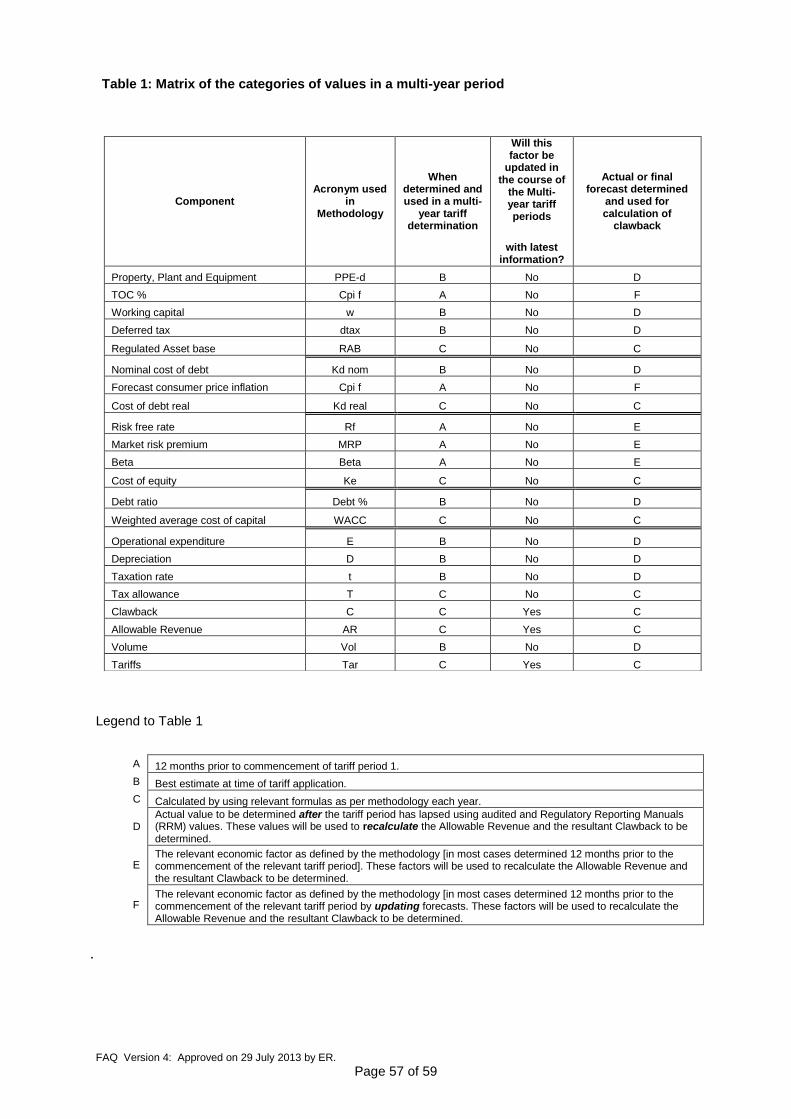
i. A matrix of the different categories of values and the timing thereof are
presented in Table 1 on the pages 57 to 72.
ii. It should be noted that clawbacks from previous tariff determinations
(single or multi-year) will still be implemented as required.

FAQ Version 4: Approved on 29 July 2013 by ER.
Page 56 of 59
8. Annexures
Annexure A:
Practical example reflecting the treatment of claw backs in a multi-year tariff
determination
FAQ Version 4: Approved on 29 July 2013 by ER.
Page 57 of 59
Table 1: Matrix of the categories of values in a multi-year period
Legend to Table 1
A 12 months prior to commencement of tariff period 1.
B Best estimate at time of tariff application.
C Calculated by using relevant formulas as per methodology each year.
D Actual value to be determined after the tariff period has lapsed using audited and Regulatory Reporting Manuals (RRM) values. These values will be used to recalculate the Allowable Revenue and the resultant Clawback to be determined.
E The relevant economic factor as defined by the methodology [in most cases determined 12 months prior to the commencement of the relevant tariff period]. These factors will be used to recalculate the Allowable Revenue and the resultant Clawback to be determined.
F The relevant economic factor as defined by the methodology [in most cases determined 12 months prior to the commencement of the relevant tariff period by updating forecasts. These factors will be used to recalculate the Allowable Revenue and the resultant Clawback to be determined.
.
Component
Acronym used in
Methodology
When determined and used in a multi-
year tariff determination
Will this factor be
updated in the course of
the Multi-year tariff periods
with latest information?
Actual or final forecast determined
and used for calculation of
clawback
Property, Plant and Equipment PPE-d B No D
TOC % Cpi f A No F
Working capital w B No D
Deferred tax dtax B No D
Regulated Asset base RAB C No C
Nominal cost of debt Kd nom B No D
Forecast consumer price inflation Cpi f A No F
Cost of debt real Kd real C No C
Risk free rate Rf A No E
Market risk premium MRP A No E
Beta Beta A No E
Cost of equity Ke C No C
Debt ratio Debt % B No D
Weighted average cost of capital WACC C No C
Operational expenditure E B No D
Depreciation D B No D
Taxation rate t B No D
Tax allowance T C No C
Clawback C C Yes C
Allowable Revenue AR C Yes C
Volume Vol B No D
Tariffs Tar C Yes C
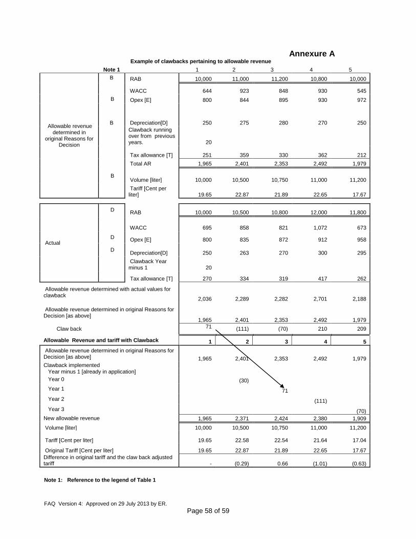
FAQ Version 4: Approved on 29 July 2013 by ER.
Page 58 of 59
Annexure A Example of clawbacks pertaining to allowable revenue
Note 1
1 2 3 4 5
Allowable revenue determined in
original Reasons for Decision
B RAB 10,000 11,000 11,200 10,800 10,000
WACC 644 923 848 930 545
B Opex [E] 800 844 895 930 972
B Depreciation[D] 250 275 280 270 250
Clawback running over from previous years. 20
Tax allowance [T] 251 359 330 362 212
Total AR 1,965 2,401 2,353 2,492 1,979
B
Volume [liter] 10,000 10,500 10,750 11,000 11,200
Tariff [Cent per
liter] 19.65 22.87 21.89 22.65 17.67
Actual
D RAB 10,000 10,500 10,800 12,000 11,800
WACC 695 858 821 1,072 673
D Opex [E] 800 835 872 912 958
D
Depreciation[D]
250
263 270 300 295
Clawback Year
minus 1 20
Tax allowance [T] 270 334 319 417 262
Allowable revenue determined with actual values for clawback
2,036 2,289 2,282 2,701 2,188
Allowable revenue determined in original Reasons for Decision [as above]
1,965 2,401 2,353 2,492 1,979
Claw back
71 (111) (70) 210 209
Allowable Revenue and tariff with Clawback 1 2 3 4 5
Allowable revenue determined in original Reasons for Decision [as above] 1,965 2,401 2,353 2,492 1,979
Clawback implemented
Year minus 1 [already in application]
Year 0
(30)
Year 1
71
Year 2
(111) Year 3
(70)
New allowable revenue
1,965 2,371 2,424 2,380 1,909
Volume [liter] 10,000 10,500 10,750 11,000 11,200
Tariff [Cent per liter] 19.65
22.58 22.54 21.64 17.04
Original Tariff [Cent per liter] 19.65 22.87 21.89 22.65 17.67
Difference in original tariff and the claw back adjusted tariff - (0.29) 0.66 (1.01) (0.63)
Note 1: Reference to the legend of Table 1