frequency analysis of extreme events

~ .

~) CHAPTER 181!;, ,

f';' FREQUENCY ANALYSIS OF

~,. EXTREME EVENTSif"

~i,

t';:

?,r;

~.';

~~ Jery R. Stedingeri; School of (:'ivil and Envir~nme.ntal Engineeringri!J; Cornell University"',i; Ithaca, New York~w

~:, Richard M. Vogel

~ Department of Civil Engineering

~ Tufts University\;;; .~" Medford, Massachusetts~,I!&~ Ef " F f I G .~l; I OU OU a- eorglou~ Department of Civil and Mineral Engineering~; University of Minnesota"~1 Minneapolis, Minnesota~~~(1~'"~~,I~i:'~'c~.~:j~

I:

Ir;,:'~B~'~;~l 18. 1 INTRODUCTION TO FREQUENCY~[ ANAL YSIS~'~~!1 Extreme rainfall events and the resulting floods can take thousands oflives and cause~ billions of dollars in damage. Rood plain management and designs for flood control~ .'orks, reservoirs, bridges, and other investigations ne~d to reflect the likelihood or~f probability of such events. Hydrologic studies also need to address the impact ofil~ unusually low stream flows and pollutant loadings because of their effects on water~ quality and water supplies.('C1-',,~~, TIlt Basic Problem. Frequency analysis is an information problem: if one had a~ sufficiently long record of flood flows, rainfall, low flows, or pollutant loadings, then~ .frequency distribution for a site could be precisely detennined, so long as change~f over time due to urbanization or natural processes did not alter the relationships of~~ concern. In most situations, available data are insufficient to precisely define the risk~~ or large floods, rainfall, pollutant loadings, or low flows. This forces hydrologists toi.~ U5C practical knowledge of the processes involved, and efficient and robust statistical

i~):i1"

--~

18.2 CHAPTER EIGHTEEN

techniques, to develop the best estimates of risk that theycan."s These techniques aregenerally restricted, with I a to 100 sample observations to estjmate events exceededwith a chance of at least I in lOO, corresponding to exceedance probabilities of Ipercent or more. In some cases, they are used to estimate the rainfall exceeded with achance of I in 1000, and even the flood flows for spillway design exceeded with achance of I in 10,000.

The hydrologist should be aware that in practice the true probability distributionsof the phenomena in question are not known. Even if they were, their functionalrepresentation would likely have too many parameters to be of much practical use.The practical issue is how to select a reasonable and simple distribution to describethe phenomenon of interest, to estimate that distribution's parameters, and thus toobtain risk estimates of satisfactory accuracy for the problem at hand.

Common Problems. The hydrologic problems addressed by this chapter primarilydeal with the magnitudes of a single variable. Examples include annual minimum7-day-average low flows, annual maximum flood peaks, or 24-h maximum precipi-tation depths. These annual maxima and minima for successive years can generallybe considered to be independent and identically distributed, making the requiredfrequency analyses straightforward.

In other instances the risk may be attributable to more than one factor. flood riskat a site may be due to different kinds of events which occur in different seasons, ordue to risk from several sources of flooding or coincident events, such as both localtributary floods and large regional floods which result in backwater flooding from areservoir or major river. When the magnitudes of different factors are independent, amixture model can be used to estimate the combined risk (see Sec. 18.6.2). In otherinstances, it may be necessary or advantageous to consider all events that exceed aspecified threshold because it makes a larger data set available, or because of theeconomic consequences of every event; such partia/ duration series are discussed inSec. 18.6.1.

18.1.1 Probability Concepts

Let the upper case letter X denote a random variab/e, and the lower case letter x apossible value of x. For a random variable X, its cumulative distribution function( cdf), denoted F x<x), is the probability the random variable X is less than or equal tox:

FX<x)=F(X$x) (18.1.1)

F x<x) is the nonexceedance probability for the value x.Continuous random variables take on values in a continuum. For example, the

magnitude of floods and low flows is described by positive real values, so that X ?; 0.The probability density function (pdf) describes the relative likelihood that a contin-uous random variable X takes on different values, and is the derivative of the cumu-lative distribution function:

fx<x) = ¥2 (18.1.2)

Section 18.2 and Table 18.2.1 provide examples of cdf's and pdf's.

FREQUENCY ANALYSIS OF EXTREME EVE"" '.3

1812 Quant;les, Exceedance P.obabil;t;es, Odds Rat;os, and ReturnPer;ods

m hydrology the p"c"'tiles 0. quontiles of a distribution are oftcn used as design"entsThe lOOp pe,centile or the plh quanlile x, is the ,alue with cumulative

p,ob,b"ity p

Fxlx,)~p (18C3)

The lOOp percentile ", is often called the 100(1- pj pe'cente'ceedanceevent be-cause ;t will be exceeded with probability I -p

The ,eturn pe,iod (sometimes called the 'eruffence inte"alj i, of\en specilied'aIhcr than the exceedance probab;lity For e,ample, (he annual maximum fIood-nowe,ceeded with a I pe,"en( probability in any yea" mchance of I in 100, i, calledIhe lOO-yea, nood In gencral, x, is the T-yea, floOd fo,

IT~- ( 1814 )I-p

Hcre are two ways that returo period can be unde"tood Fi,," in a fixed T-yea,"riod the expected numbe, ofe,ceedaoce, of(he T-yea, even( ffi e,act;y I, if tiredi,(ribution of flood, does no( change ovcr (h,t period (hw on avcrage one floOdgrea(e, (h,n the T-yea, flood Ie,cl ocr"" in a T-yea, pe,iod

Ahemativcly, iffloods a,e independent f,om yea, to year, (he p,oh,b;lity Ihat thefi"I e,ceedance oflevcl x, occurs in yea, k ;s the p,obability of(k -I) years wilhoulaa e'ceed,nce followed by a year in which the value of x ex=d,x,

P(exacIlykycarsuntiIX"x,j~p'-'(I-p} (18C5)

Thisi,ageometric d;stribut;on with mean 11(1- p} Thu,(he a'emgctime until thelevclx,ffie,ceededequai, Tyears Howeve" the p'obability(hat x, i, not excceded ina T-yea",riod ffipr~(1 -IIT)', which for 11(1 -p)~ T" 25 isapprox;matelyJ6J ","ent, mabout a chance of I in 3

Return "riod is a meam of exprcs,;ng the exceed,nce p,obabilily Hyd,olog;s(,one, ""k of the 20-yea, nood or the I 000-yea, ,ainfal;, ,athcr (han evenl' exceeded.;Ih p,obabililiesof5 0'0! pe,cent in any yea" conespondingto chances of I in 20,°,ofl in 1000 Rctum penodhasbeen inco"ecllyunderstood to mean Ihatone andoaly one T-year event should occu, e'ery T years Actually, (he p,obability of theTye,r nood being exceeded i, IITin every yeac The awkwa,dnes' of small proba-bililie"nd the inconect ;mpliea(ion ofretum periods can both be avoided by report-;'godds mtivslhwthe I pe,eentexceedance eveulcan be described a, a value with aI i, 100 chance of being exceeded each yeac

1813 P.oduct Moments and the;, Sample Estimatoffi

Se'eral summary statist;cs can de",;be the cha,acte, of the p,ohab;lity d;stribulionor a candom variabk Moment, and quanliles a,e u"d 10 de,cribe the iocation OC'"trnl kndency of a candom variable, and ;,' 'p,ead, as deocribed ;n Sec 172 andr,ble 17LC The mean ofa rnndom variable X is defined as

~ !'x~E[X] (1816)


The second moment about the mean is the variance, denoted Var {X) or 0"1- where

ai= Var (X) = E[(X-px)2] (18.1.7)

The standard deviation 0" x is the square root of the variance and describes the widthor scale of a distribution. These are examples of product moments because theydepend upon powers of X.

A dimensionless measure of the variability in X, appropriate for use with positiverandom variables X ~ 0, is the coefficient of variation, defined in Table 18.1.1. Table18.1.1 also defines the coefficient of skewness Yx, which describes the relative asym-metry of a distribution, and the coefficient of kurtosis, which describes the thicknessof a distribution's tails.

Sample Estimators. From a set of observations (XI, ..., Xn), the moments of adistribution can be estimated. Estimators of the mean, variance, and coefficient ofskewness are

-n X,f1x=X= L -!.

;-1 n

n

L {X; -X)2

a-1-=S2=[~] {18.1.8)

nn 2: {X; -X)3

y =G= ;-1x {n- 1){n -2)S3

TABLE 18.1.1 Definitions of Dimensionless Product-Moment and L-Moment Ratios

Name Denoted

Product-moment ratios

Coefficient of variation CV x ax/Jlx

E(X- )3Coefficient of skewness. Yx 311xax

E(X- )4Coefficient of Kurtosisf -at-

L-moment ratios

L-coefficient of variation* L-CV,1"2 A.2/A.,L-coefficient of skewness L-skewness, TJ A.J/).2L-coefficient of kurtosis L-kurtosis, T4 A.4/ ).2

.Some texts define .81 = [Yxr as a measure of skewness.t Some texts define the kurtosis as {E[{X -.Ux)4]!ai -3}; others use

the term excess kurtosis for this difference because the nonnal distribu-tion has a kurtosis of 3.

.Hosking 72 uses r instead of -r2 to represent the L-CV ratio.

FREQUENCY ANAL YSIS OF EXTREME EVENTS 18.5

Some studies use different versions of fJi- and y x that result from replacing (n -1 )and (n -2) in Eq. ( 18.1.8) by n. This makes relatively little difference for large n. Thefactor (n -1) in the expression for uk yields. an unbiased estimator of the varianceO'l. The factor n/[(n -I )(n -2)] in expression for rx yields an unbiased estimator ofE[(X-Jl.x)3], and generally reduces but does not eliminate the bias ofyx(Ref. 159).Kirby84 derives bounds on the sample estimators of the coefficients of variation andskewness; in fact, the absolute value ofboth S and G cannot exceed .fii for the sampleproduct-moment estimators in Eq. ( 18.1.8).

Use of Logarithmic Transformations. When data vary widely in magnitude, as oftenhappens in water-quality monitoring, the sample product moments of the logarithmsof the data are often employed to summarize the characteristics of a data set or toestimate parameters of distributions. A logarithmic transformation is an effectivevehicle for normalizing values which vary by orders of magnitude, and also forkeeping occasionally large values from dominating the calculation of product-moment estimators. However, the danger with use of logarithmic transformations isthat unusually small observations ( or low outliers) are given greatly increased weight.This is a concern if it is the large events that are of interest, small values are poorlymeasured, small values reflect rounding, or small values are reported as zero if theyfall below some threshold.

18.1.4 L Moments and Probability-Weighted Moments

L moments are another way to summarize the statistical properties of hydrologicdata.72 The first L-moment estimator is again the mean:

).,=E[X] (18.1.9)

Let X(lln) be the ith-largest observation in a sample of size n (i = I corresponds to thelargest). Then, for any distrib~tion, the second L moment is a description or scalebased on the expected difference between two randomly selected observations:

).2 = t E[X(112) -X(212)] (18.1.10)

; Similarly, L-moment measures of skewness and kurtosis use

).3 = t E[X(113) -2X(213) + X(3f3)]

(18.1.11)).4 = t E[X(lf4) -JX(214) + JX(314) -X(414)]

as shown in Table 18.1.1.

Advantages of L Moments. Sample estimators of L moments are linear combina-tions (hence the name L moments) of the ranked observations, and thus do notinvolve squaring or cubing the observations as do the product-moment estimators inEq. ( 18.1.8). As a result, L-moment estimators of the dimensionless coefficients ofvariation and skewness are almost unbiased and have very nearly a normal distribu-tion; the product-moment estimators of the coefficients of variation and ofskewnessin Table 18.1.1 are both highly biased and highly variable in small samples. BothHosking72 and Wallis'63 discuss these issues. In many hydrologic applications anoccasional event may be several times larger than other values; when product mo-

;.';i" ments are used, such values can mask the information provided by the other observa-

~f~

1 B. 6 CHAPTER EIGHTEEN

tions, while product moments of the logarithms of sample values can overemphasizesmall values. In a wide range of hydrologic applications, L moments provide simpleand reasonably efficient estimators of the characteristics of hydrologic data and of adistribution's parameters.

L-Moment Estimators. J ust as the variance, or coefficient of skewness, of a randomvariable are functions of the moments E[X], E[X2], and E[X3]," L moments can bewritten as functions of prohahility-weighted moments (PWMS),48.72 which can bedefined as

Pr = E{X [F(X)]r) (18.1.12)

where F(X) is the cdf for X. Probability-weighted moments are the expectation of Xtimes powers of F(X). (Some authors define PWMs in terms of powers of[ 1 -F(X)].)For r = 0, Po is the population mean Jlx.

Estimators ofL moments are mostly simply written as linear fungions of estima-tors ofPWMs. The first PWM estimator ho of Po is the sample mean X in Eq. ( 18.1.8).

To estimate other PWMs, one employs the ordered observations, or the orderstatistics X(n) ~ ...~X(I)' corresponding to the sorted or ranked observations in asample (X;li = 1, ..., n). A simple estimator of Pr for r ~ 1 is

hr* = .!. i X(j) r 1 -(j -o.35)lr (18.1.13)n j= I L n J

where 1 -(j -0.35}/n are estimators of F(X(j)}. hr* is suggested for use when esti-mating quantiles and fitting a distribution at a single site; though it is biased, itgenerally yields smaller mean square error quantile estimators than the unbia5(.'destimators in Eq. (18.1.14) below.68.89

When unbiasedness is important, one can employ unbiased PWM estimators

ho=Xn-1 (n -j)X .b = ~ ~,. J 1./1.(j)

I £J n( n- I )j-1 (18.1.14)

n-2 (n -j) (n -j -l)X "b = ~ ~~J J I \'J J '1./I.U>2 j~1 n(n- l)(n -2)

b = n-3 (n -j) (n -j -1) (n -L -2)X(j)

3 j~1 n(n- l)(n -2)(n -3}

These are examples of1he general formula

( n -j\ ( n -j\-I n -, \ r ) XU) 1 n -, \ r ) XU)

P,=br=- Ln = L -cr (18.1.15) nj-1 n-1 (r+ l)j=l n

r r+1

for r= I, ..., n- I [see Ref. 89, which defines PWMs in terms of powers 0(( I -F)J; this formula can be derived using the fact that (r + 1 )P, is the expected valueof the largest observation in a sample of size (r + 1 ). The unbiased estimators arerecommended for calculating L moment diagrams and for use with regionalization

procedures where unbiasedness is important.

-


For any distribution, L moments are easily calculated in tenns of PWMs from

).1 = Po

).2 = 2Pf -Po

(18.1.16)).3 = 6P2 -6Pl +Po

).4 = 20P3 -30P2 + 12p/ -Po

Estimates of the ).j are obtained by replacing the unknown Pr by sample estimators brfrom Eq. (18.1.14). Table 18.1.1 contains definitions of dimensionless L-momentcoefficients of variation T 2, of skewness T J , and of kurtosis !4. L-moment ratios arebounded. In particular, for nondegenerate distributions with finite means, I !rl < 1 forr = 3 and 4, and for positive random variables, X> 0, O < T2 < I. Table 18.1.2 gives

expressions for )./ , A2, ! J , and !4 for several distributions. Figure 18.1.1 shows rela-lionships between T3 and T4. (A library of FORTRAN subroutines for L-momentanalyses is available; 74 see Sec. 18.11. ) .

Table 18.1.3 provides an example of the calculation of L moments and PWMs.The short rainfall record exhibits relatively little variability and almost zero skew-ness. The sample product-moment CY for the data of 0.25 is about twice the L-CY !2equal to 0.14, which is typical because )..2 is often about half of a.

L-Moment and PWM Parameter Estimators. Because the first r L moments arelinear combinations of the first r PWMs, fitting a distribution So as to reproduce thefirst r sample L moments is equivalent to using the corresponding sample PWMs.Infact, PWMs were developed first in terms of powers of ( I -F) and used as effectivestatistics for fitting distributions.89.90 Later the PWMs were expressed as L momentswhich are more easily interpreted.72./28 Section 18.2 provides formulas for the pa-rameters of several distributions in terms of sample L moments, many of which areobtained by inverting expressions in Table 18.1.2. (See als~ Ref. 72.)

18.1.5 Parameter Estimation

Fitting a distribution to data sets provides a compact and smoothed representation ofthe frequency distribution revealed by the available data, and leads to a systematicprocedure for extrapolation to frequencies beyond ~he range of the data set. Whenflood flows, low flows, rainfall, or water-quality variables are well-described by somefamily of distributions, a task for the hydrologist is to estimate the parameters e ofthat distribution so that required quantiles and expectations can be calculated withthe "fitted" model. For example, the normal distribution has two parameters, .u andDl. Appropriate choices for distribution functions can be based on examination ofthe data using probability plots and moment ratios (discussed in Sec. 18.3), thephysical origins of the data, previous experience, and administrative guidelines.

Several general approaches are available for estimating the parameters of a distri-bution. A simple approach is the method of moments. which uses the availableA .sample to compute an estimate e of e so that the theoretical moments of thedistribution of X exactly equal the corresponding sample moments described in Sec.18.1.3. Alternatively, parameters can be estimated using the sample L momentsdjscussed in Sec. 18.1.4, corresponding to the method of L moments.

Still another method that has strong statistical motivation is lhe method of ma..\'i-mum likelihood. Maximum likelihood estimators (MLEs) have very good statistical

1 8.8 CHAPTER EIGHTEEN

TABLe 18.1.2 Values ofL Moments and Relationships for the Inverse of the cdfforSeveral Distributions

Distribution and inverse cdf L moments"

p+a. p-aUniform: ).1 = ~ ).2 = ~

x = a + <P -a)F T3 = T4 = 0

IIExponential:* ).1 = t. + p ).2 = 2P

In [ 1 -FJ IIx = ~ -T3 = -T4 = -

p 3 6

(1Norrnalt ).1 =JL A2 = ~

x = JL + (1<!>-I[FJ T3 = 0 T4 = 0.1226

Gumbel: ).1 = ~ + 0.5772 a ).2 = a In 2x = t. -a In [-In F] !3 = 0.1699 T4 = 0.1504

a aGEV: ).1=t.+-{I-r[I+K]} ).2=-(1-2-I()r(I+K)

K K

a .{2(1 -3-1() }x = ~ + -{ I -[ -In F]1 T 3 = --3K (1-21

1- 5(4-K) + 10(3-1- 6(2-1T4 = I -2-1(

a aGeneralized Pareto: ).1 = ~ + m ).2 = (I + K)(2 + K)

a 1 -K ( I -K)(2 -K)

x=~+K{I-[I-F]1 T3=3"+K T4=(3+K)(4+K)

Lognormal See Eqs. (18.2.12), (18.2.13)

Gamma See Eqs. (18.2.30), (18.2.31)

.Alternative parameterization consistent with that for Pareto and GEV distributions is:x = f. -a In[ I -F] yielding A.1 = f. + a; A.2 = a/2.

t $-1 denotes the inverse of the standard normal distribution (see Sec. 18.2.1 ).Note: F denotes cdf F x<x).Source: Adapted from Ref. 72, with corrections.

properties in large samples, and experience has shown that they generally do well

with records available in hydrology. However, often MLEs cannot be reduced to

simple formulas, so estimates must be calculated using numerical methods.8s MLEssometimes perfonn poorly when the distribution of the observations deviates in

significant ways from the distribution being fit.

A different philosophy is embodied in Bayesian inference, which combines prior

infonnation and regional hydrologic information with the likelihood function foravailable data. Advantages of the Bayesian approach are that it allows the explicitmodeling of uncertainty in parameters, and provides a theoretically consistentframework for integrating systematic flow records with regional and other hydrologicinfonnation.3.88.127.lso

1 8.1 O CHAPTER EIGHTEEN

Occasionally nonparametric methods are employed to estimate frequency rela.tionships. These have the advantage that they do not assume that floods are drawnfrom a particular family of distributions.2.7 Modern nonparametric methods havcnot yet seen much use in practice and have rarely been used officially. However,curve-fitting procedures which employ plotting positions discussed in Sec. 18.3.2 arcnonparametric procedures often used in hydrology.

Of concern are the bias, variability, and accuracy of parameter estimaton8[x. , ...,Xn], where this notation emphasizes that an estimator 8 is a randomvariable whose value depends on observed sample values {XI' ...Xn). Studies 01estimators evaluate an estimator's bias, defined as

Bias [8] = E[8] -8 (18.1.17;

and sample-to-sample variability, described by Var [8]. One wants estimators tobcnearly unbiased so that on average they have nearly the correct value, and also t<Jhave relatively little variability. One measure of accuracy which combines bias andvariability is the mean square error, defined as

A A A AMSE [8] = E[(8 -8)2] = {Bias [8])2 + Var [8] (18.1.18;

An unbia,fjed estimator (Bias [8] = 0) will have a mean square error equal to i~variance. For a given sample size n, estimators with the smallest possible mean squarcerrors are said to be efficient.

Bias and mean square error are statistically convenient criteria for evaluatin@estimators of a distribution's parameters or of quantiles. In particular situations'hydrologists can also evaluate the expected probability and under- or overdesign, 01use economic loss functions related to operation and design decisions.112,124

18.2 PROBABILITY DISTRIBUTIONS FOREXTREME EVENTS

This section provides descriptions of several families of distributions commonly usedin hydrology. These include the normal/lognormal family, the Gumbel/Weibul11generalized extreme value family, and the exponential/Pearson/log-Pearson type 3family. Table 18.2.1 provides a summary of the pdf or cdf of these probabilitydistributions, and their means and variances. (See also Refs. 54 and 85.) The Lmoments for several distributions are reported in Table 18.1.2. Manyotherdistribu.tions have also been successfully employed in hydrologic applications, including thcfive-parameter Wakeby distribution,69,75 the Boughton distribution, 14 and the TCEVdistribution (corresponding to a mixture of two Gumbel distributions I 19).

18.2.1 Normal Family: N. LN. LN3

The normal (N), or Gaussian distribution is certainly the most popular distributionin statistics. It is also the basis of the lognormal (LN) and three-parameter lognormal(LN3) distributions which have seen many applications in hydrology. This sectiondescribes the basic properties of the normal distribution first, followed by a discus-sion of the LN and LN3 distributions. Goodness-of-fit tests are discussed in Sec. 18.3and standard errors of quantile estimators in Sec. 18.4.2.

iff~fI ;1, FREQUENCY ANAL YSJS OF EXTREME EVENTS 1 8.11

,,"",,~i'c~1~\ Tilt Normal Distribution. The normal distribution is useful in hydrology for de-~~f scribing well-behaved phenomena such as average annual stream flow, or average1!,:f~-" annual pollutant loadings. The central limit theorem demonstrates that if a random[:r: variable X is the sum of n independent and identically distributed random variables;;,~~ \\cith finite variance, then with increasing n the distribution of X becomes normal~;1,~ rtgardless of the distribution of the original random variables.I~~!C The pdf for a normal random variable X is~:f§i;;:r,:i I l I ~ x -J1 )2

Jit.;~;,' fX<x) = exp --x (18.2.1)~!,'j}, v'2;tUt 2 u x,,'~!7 .x

~JI~t: X is unbounded both above and below, with mean .Ux and variance uk. The normal.!~#i; distribution's skew coefficient is zero because the distribution is symmetric. The~1~; product-moment coefficient of kurtosis, E[(X- .UX)4]/U4, equals 3. L moments are~r~~'c given in Table 18.1.2.i;c~ The two moments of the normal distribution, Jlx and uk, are its natural parame-i];i![ ters. They are generally estimated by the sample mean and variance in Eq. ( 18.1.8);;i; these are the maximum likelihood estimates if ( n -I) is replaced by n in the denomi-\t";\~, nator of the sample variance. The cdf of the normal distribution is not available inIJi;! closed form. Selected points Zp for the standard normal distribution with zero mean~;~, and unit variance are given in Table 18.2.2; because the normal distribution isc symmetric, Zp = -ZI-p.

An approximation, generally adequate for simple tasks and plotting, for the stan-dard normal cdf, denoted q,(z), is

r (83z + 351)z + 5621ii;: q,(z) = I -0.5 exp L- 7031z + 165 J (18.2.2)

:i;~ ..;"~,f for O < z :5 5. An approximatIon for the Inverse of the standard normal cdf, denoted..'~"" I .\:i,:.;',,~: 4»- (p) IS,,:~,,1;rt"'C 1!1"-:'

.1. t'i',c",1

~!~~;;;, p O.13S - ( I - p) O.13S

~~!,"' -I 8.:lfif; q, (p) = Zp = 0 1975 (I .2.3a)I"',""~tl]c .

:;(;W or the more accurate expression valid for 10-7 <p < 0.5;~i; -I = =- I y2[(4y+100)y+205]

q, (p) Zp -y [(2y + 56)y + 192]y + 131 ( 18.2.3b)

where y = -In (2p). [Eqs. (18.2.2) and (18.2.3b) are from Ref. 35.]

~', Lognormal Distribution. Many hydrologic processes are positively skewed and are:1:! nol nonnally distributed. However, in many cases for strictly positive random vari-!:l~j abies X > 0 their logarithm:!;!"'h ,~~f'WJ~' y= In (X) (18.2.4)

t~,

::'~(; is well-described by a normal distribution. This is particularly true if the hydrologic, variable results from some multiplicative process, such as dilution. Inverting Eq.

( J 8.2.4) yields

"'c x= exp (Y)i,;'

~f~:

TABLE 18.2.1 Commonly Used Frequency Distributions in Hydrology (see also Table 18.1.2)

Distribution pdfand/orcdf Range Moments

I [ I (X-JlX )2]Normal fX<x)=-exp ~<x<~ Jlxandqi;Jlx=O

~ 2 O'x

I [ I (In(X) -JlY )2] ( q~)Lognormal* fx<x) = exp --x > 0 Jlx = exp JlY + 2x~ 2 qy

qi = Jli[exp (q~) -1]

Jlx= 3CVx+CV;

Pearson type 3 fX<x) = IPI[P(x -{)]a-1 exp [~~ -,)] a > 0 Jlx = , + i; qi = ~

2r(a) is the gamma function for P > 0: x > , and Jlx = ~

-2(for P > 0 and, = 0: Yx = 2 CV x) for P < 0: x < , and Yx -~

exp {-p[ln (x) -c;]}log-Pearson type 3 fX<x) = LPKP[ln (x) -c;]}a-1 xr(a) See Eq. (18.2.34)

for p< 0, 0 <x< exp (,); for p> 0, exp {,) <x < ~

IIExponential fx<x) =.8exp [-.8(x- ,)] x> ,for.8> 0 Jlx='+p; O"k=p2

FZ<x)-l-exp{-P(x-~)} "x-2

I [ x-~ ( x-~ )]Gumbel fx<x) -;;- exp -a- -exp -a- -~ < x < ~ Jlx- ~ + O.5772a

[ ( x- ~)] 1r2a2FX<x)=exp -exp --a- O"i=6=1.645a2;yx=I.1396

{ [ K{X- ,) ] I/K } (a)GEV F x<x) = exp -I -a {q; exists for K > -0.5) Jlx = , + K [I -r(1 + K)]

when K> 0, X< ( ,+~); K< 0, X> ( ,+~) q}= (~)2{r(1 + 2K) -[r(1 +.K)]2}

Weibull fX<x) = (~) (~)"-I exp [ -(~)"] x> O;a, k>O .ux=a r ( I +i)

FX<x)= I-exp [-(x/a)"] q}=a2{r( I+i)-[ r( l+i)J}

( I ) [ (x- ,) ]I/K-I aGeneralized Pareto fx<x) = -I -/C- .forK<O, 'sx< ~ .Ux='+-

a a (1 + K)

[ (X-,) ] I/~ a FX<x) = 1- 1- K-a- forK>O, ,sxs'+K 0"}= a2/[(1 + /C)2(1 + 2K)]

2(1- K)(I + 2K)I/2(Yxexistsfor/C>-0.33) Yx= (1 + 3/C)

.Here y -In (X). Text gives formulas for three-parameter lognormal distribution, and for two- and three-parameter lognormal with common base 10logarithms.


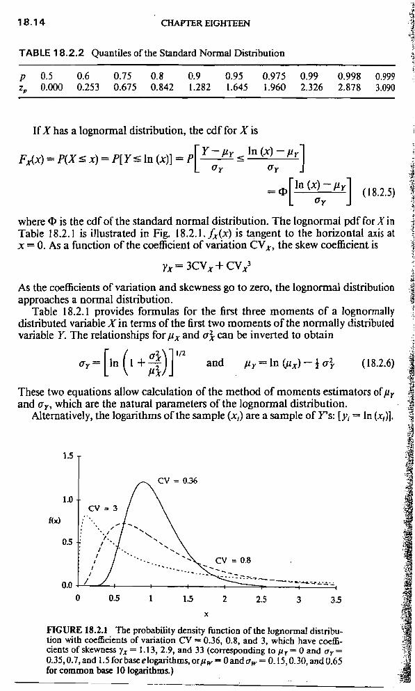
TABLe 18.2.2 Quantiles of the Standard Normal Distribution

p 0.5 0.6 0.75 0.8 0.9 0.95 0.975 0.99 0.998 0.999Zp 0.000 0.253 0.675 0.842 1.282 1.645 1.960 2.326 2.878 3.090

If X has a lognonDal distribution, the cdf for X is

F x<x) = P(X~ x) = P[Y~ In (x)] = pr.!::=f-r ~ In (x) -Jly 1

L ay ay J

="'[~] (18.2.5)

where <1> is the cdf of the standard nonDal distribution. The lognonDal pdf for X inTable 18.2.1 is illustrated in Fig. 18.2.1. f x(x) is tangent to the horizontal axis atx = 0. As a function of the coefficient of variation CY x, the skew coeffIcient is

rx= 3CY x+ CY xJ

As the coefficients of variation and skewness go to zero, the lognonDal distributionapproaches a nonDal distribution.

Table 18.2. I provides fonDulas for the first three mQments of a lognonnallydistributed variable X in tenDS of the first two moments of the nonD'aUy distributedvariable Y. The relationships forJlx and a} can be inverted to obtain

r { a2 \ 11/2ay=Lln\I+17iJJ and Jly=ln(jlx)-ta} (18.2.6)

These two equations allow calculation of the method of moments estimators of/lrand ay, which are the natural parameters of the lognonDal distribution.

Alternatively, the logarithms of the sample (xi) are a sample of Y's: [Yi = In {Xu].

1.5

cy = 0.36

1.0CV=3

f(x) : .., ..., , /: ...I

05 : ,..., .II

( .~ ..8( ..~...~

I .-/ ..~...~0.0 --~~ "'"'".:.'.=.--Z

0 0.5 1 1.5 2 2.5 3 3.5

x

FIGURE 18.2.1 The probability density function of the lognormal distribu-bon with coefficients of variation cy = 0.36, 0.8, and 3, which have coeffi-cients of skewness yx = 1.13, 2.9, and 33 (corresponding to Jly = O and O"y =

0.35,0.7, and 1.5 forbaseelogarithms,or,llw= Oandt1w= 0.15,0.30, andO.65for common base 10 logarithms.) ,

FREQUENCY ANALYSIS OF EXTREME EVENTS 18.15

The sample mean and variance of the observed (Y,), obtained by using Eq. (18.18),are the maximum-Iikelihood estimators of the log~omlal distribution's parameters if(n- I) is replaced by n in the denominator of 4. The moments of the Y:s are botheasier to compute and generally more efficient than the moment estimators in Eq.(18.2.6), provided the sample does not include unusually small values;'26 see discus-sion of logarithmic transfomlations in Sec. 18.1.3.

Hydrologists often use common base 10 logarithms instead of natural logarithms.Let Wbe the common logarithm of X, log (X). Then Eq. (18.2.5) becomes

FX<X)=P[ ~S 10g(X)-Jlw ] =<1> [log(X) -Jlw

](Jw (Jw (Jw

The moments of X in terms of those of Ware

Jlx= IO"w+ID('oJo'wI2 and (Ji=Jli(IOID(loJo'w-l) (18.2.7)

where In(10) = 2.303. These expressions may be inverted to obtain:

[10 (1+(J2/2) ] 1/2 uw= g In(IO)JlX and Jlw=log(Jlx)-!ln(10)(J1v (18.2.8)

Three-Parameter Lognormal Distribution. In many cases the logarithms of a ran-dom variable X are not quite normally distributed, but subtracting a lower boundparameter.; before taking logarithms may resolve the probleril. Thus

Y=ln(X-c;) (18.2.9a)

is modeled as having a nomlal distribution, so that

X=.;+exp(Y) (18.2.9b)

For any probability level p, the quantile Xp is given by

xp=.;+exp(Jly+(JyZp) (18.2.9c)

In this case the first two moments of X are

Jlx=.;+exp(jly+!(Jj.) and (Ji=[exp(2Jly+(J})][exp«(J})-I]

(18.2.10a)

with skewness coefficient

Yx=31J+1JJ

where 1J = [ exp( (J} ) -I ]05. If common base 10 logarithms are employed so that

W= log (X- .;), the value of.; and the fomlula for Yx are unaffected, but Eq.(18.2.10a) becomes

Jlx=.;+ 10"w+In(10)a'wI2 and (Ji=(jlx-.;-)'1J2 (18.2.10b)

with 1> = (10In(loJo'wI2 -1)05.

Method-of-moment estimators for the three-parameters lognomlal distributionare relatively inefficient. A simple and efficient estimator of.; is the quanlile-lawer-bound eslimalar

x x -X2p ~= ~(I)~(n) -~m-D (18.2.11) X(I) + X(n) 2xm-D

-

r

~p1 8.1 4 CHAPTER EIGHTEEN 'I'.."

"~~

TABLE 18.2.2 Quantiles of the Standard Normal Distribution ;~0?(.~~

p 0.5 0.6 0.75 0.8 0.9 0.95 0.975 0.99 0.998 0,999 -~iZp 0.000 0.253 0.675 0.842 1.282 1.645 1.960 2.326 2.878 3.090 ';

~,j\:~

If X has a lognonnal distribution, the cdf for X is ~-;4'

Ly -11 In (x) -11 ] ~FX<x) = P(X~ x) = P[Ys In (x)] = p y ~ y ~

ay ay ,i

=t1>r~ 1 (18.2.5) iiL ay J '~

1..,where <1> is the cdf of the standard nonnal distribution. The lognormal pdf for X in ~dTable 18.2.1 is illustrated in Fig. 18.2.1. J x(x) is t3;ngent to the horizontal axis at '~x = 0. As a function of the coefficient of variation cy x' the skew coefficient is ~

c~Yx= 3CY x+ CY X3 i1

;.i

As the coefficients of v~ria~ion. and skewness go to zero, the lognormal distribution :japproaches a nonnal dlstnbutlon. :~

Table 18.2.1 provides fonnulas for the first three moments of a lognormally ~distributed variable X in tenns of the first two moments of the normally distributed .~

1variable Y. The relationships forl1x and ai can be inverted to obtain -;

",,;

ay=r1n(1+4\11/2 and Jly=ln(ux)-!a} (18.2.6) IL \ JlxJJ ,~

~1These two ~quations allow calculation of the method of mon;ten.ts e~timators of 'Ur jand a y, which are the natural parameters of the lognormal distnbutlon. ~

Alternatively, the logarithms of the sample (xi) are a sample of rs: [Yi = In (Xi)]. ~,~

~~.,~,'.;15 ~~ ..;':ji

t

~1.0

1cv = 3 ;,'- ~

..:f(x) :' .." ~

I' ./ '""-. I ".

, .: I.. ;I¥ 0.5 I .1~

I c

, 8 .~

I' -,

, :;

I 11;! -:--"T~ ,.-00 / --~ : :. ., ,\#

0 0.5 1 1.5 2 2,5 3 3.5 ~

'~"'

1~GU~ 18.2.1. The prob~b~ty densityxfunctiOn of the logn.ormal distribu- ~bon Wlth coeffiCIents of vanabon CY = 0.36, 0.8, and 3, which have coeffi- :~,. f 2 .,'!J Clents O skewness Yx = 1.13, ..9, and 33 (corI"esponding to 'Uy = O and ay = ;;~

0.35,0.7,and 1.5 for base eloganthms,orJlw = OandO'w = O.15,0.30,andO.651 c,\;

for common base 10 logarithms.) ';~

-;

FREQUENCY ANALYSIS OF EXTREME EVENTS 18.15

.he sample mean and variance of the observed (yJ, obtained by using Eq. ( [8.1.8),re the maximum-likelihood estimators of the logl)onual distribution's parameters if, -I) is replaced by n in the denominator of sly. The moments of the y,'s are bothasier to compute and generally more efficient than the moment estimators in Eq.18.2.6), provided the sample does not include unusually small values;"' see discus-on of logarithmic transfonuations in Sec. 18.1.3.

Hydrologists often use common base 10 logarithms instead of natural logarithms.et Wbe the common logarithm of X, log (X). Then Eq. (18.2.5) becomes

FX<X)=P[ ~'; log(X)-JJw] =fl> [log(X)-JJw

](Jw (Jw (Jw

he moments of Xin tenus of those of Ware

JJx= lOU.+In(lo>a'.I' and (Ji=J1i(101n('°>a'.-I) (18.2.7)

here In(IO) = 2.303. These expressions may be inverted to obtain:

[IOg(I+(J'/JJ') ]II' "w= x x and JJw=log(J1x)-!ln(IO)(JJv (18.2.8)

In(IO)

\ree-Parameter Lognormal Distribution. In many cases the logarithms of a ran-Jm variable X are not quite normally djstributed, but subtrac;ting a lower boundIrameter ~ before taking logarithms may resolve the problem. Thus

Y=ln (X-fJ (18.2.9a)

modeled as having a nonual distribution, so that

X=~+exp(Y) (18.2.9b)

Jr any probability level p, the quantile Xp is given by

xp=~+exp(J1y+(JyZp) (18.2.9c)

this case the first two moments of X are

=<;+exp(J1y+!(Jj,) and (Ji=[exp(2J1y+(Jj,)][exp«(Jj,)-I]

(18.2.10a)

lh skewness coefficient

Jlx=3<p+<pJ

iere .p = [exp«(J}) -1]0'. If common base 10 logarithms are employed so that= log (X- I'.), the value of I'. and the formula for Yx are unaffected, but Eq.

\.2.10a) becomes

J1x=~+ lOU.+In(IO)u'.I' and (Ji=(J1x-I'.)'.P' (18.2.10b)

h.p=(tO'n(JO>a'.t'-l)Q,.Method-of-moment estimators for the three-parameters lognonual distributionrelatively inefficient. A simple and efficient estimator of I'. is the quantile-lower-Ind estimator:

{~ X(I)XW-X~odian (18.2.11)X(I) + X~=" -~-


when X(I) + X(n) -2xmedian > 0, where X(I) and X(n) are, respectively, the largest andsmallest observed values; Xmedian is the sample medium equal to X(k+ I) for odd samplesizes n = 2k + 1, and 1(X(k) + X(k+ I» for even n = 2k. [When X(I) + X(n) -2xmedian <

0, the formula provides an upper bound so that In( ~ -x) would be normally distrib-uted.] Given ~, one can estimate)1yand cr}by using the sample mean and varianceof Yi = In (xi -~), or wi = log (xi -~). The quantile-lower-bound estimator's per.fonnance with the resultant sample estimators of)1 y and 0-} is better than method-of.moments estimators and competitive with maximum likelihood estimators.61.126

For the two-parameter and three-parameterlognormal distribution, the second Lmoment is

A.2 = exp ~ )1y + -1 ) erf~ ~ ) = 2 exp ~ )1y + -1 ) L (f>~ -Ji) -~J (18.2.12)

The following polynomial approximates, withiaO.0005 forIT31<0.9, the relationship'between the third and fourth L-moment ratios, and is thus useful for comparingsample values of those ratios with the theoretical values for two- or three-parameterlognonnal distributions: 73

T4 = 0.12282 + 0.77518 T~ + 0.12279 -r1- 0.13638 T~ + 0.11368 'l"~ (18.2.13)

18.2.2 GEV Family: Gumbel, GEV, Weibull .

Many random variables in hydrology correspond to the maximum of several similarprocesses, such as the maximum rainfall or flood discharge in a year, or the loweststream flow. The physical origin of such random variables suggests that their distri.bution is likely to be one of several extreme value (EV) distributions described byGumbel.51 The cdf of the largest of n independent variates with common cdf F(.~) issimply F(x)n. (See Sec. 18.6.2.) For large n and many choices for F(x), F(x)" con.verges to one of three extreme value distributions, called types I, II, and III. Unfor1u-nately, for many hydrologic variables this convergence is too slow for this argumentalone to justify adoption of an extreme value distribution as a model of annualmaxima and minima.

This section first considers the EV type I distribution, called the Gumbel distribu.tion. The generalized extreme value distribution (GEV) is then introduced. It spansthe three types of extreme value distributions for maxima popularized by Gum.bel.68.8° Finally, the Weibull distribution is developed, which is the extreme value tYJXIII distribution for minima bounded below by zero. Goodness-of-fit tests are dis-cussed in Sec. 18.3 and standard errors of quantile estimators in Sec. 18.4.4.

The Gumbel Distribution. Let MI, ..., M n be a set of daily rainfall, stream flow,or pollutant concentrations, and let the random variableX= max (Mi) be the ma,j.mum for the year. If the Mi are independent and identically distributed randomvariables unbounded above, with an "exponential-like" upper tail ( examples includethe normal, Pearson type 3, and lognormal distributions), then for large n the variattX has an extreme value type I distribution, or Gumbel distribution.3.51 For example,the annual-maximum 24-h rainfall depths are often described by a Gumbel distribu.tion, as are annual maximum stream flows.

The Gumbel distribution has the cdf, mean, and variance given in Table 18.2.1.and corresponding L moments are given in Table 18.1.3. The cdfiseasily inverted toobtain

Xp = ~ -a In [-In (p)] (18.2.

,

!

¥;

1 8.18 CHAPTER EIGHTEEN ii}:

,

'~~

order r PWM Pr of a GEV distribution is ;;;

!

Pr=(r+ 1)-lt~+;ll -mJJ (18.2.20) f~

,

F"

L moments for the GEV distribution are given in Table 18. 1.2. :+;

For 0 :5 <5 :5 I, a good approximation of the gamma function, useful with Eqs. ~:

(18.2.19) and (18.2.20) is .i~

5 ,¥~

,~

r(1 + <5) = I + L a;<5i + E (18.2.21) :~~

i= I ,~";

where a l = -0.5748646 :fiq

,

a2 = 0.951 2363 ~'

c;"

a3 = -0.6998588 t~

c'c

a4 = 0.424 5549 '~j

a =-0.1010678 ;,

5 ct

~1,-

with lei :5 5 X 10-5 [Eq. (6.1.35) in Ref. I]. For larger arguments one can use the ~,

relationship r(1 + w) = wr(w) repeatedly until 0 < w < I; for integer "', ,~

r( I + w) = w! is the factorial function. ~~

The parameters of the GEV distribution in terms of L moments are68 :l

,it

K = 7.8590c + 2.9554c2 ( 18.2.220) {,

K}..2

a = r(1 + K) (1 -2-K) (18.2.22b)

+ a rr(, t K') -11

~ = }..1 ~ ~[~:J.<f ] ( 18.2.22c)

where

2}..2 In (2) 2PI -Po In (2)

c=--=-

}..3 + 3}..2 In (3) 3P2 -Po In (3)

The quantiles of the GEV distribution can be calculated from

a "

Xp = ~ + -{1- [-In (p)]K} (18.2.23)

K :'

where p is the cumulative probability of interest. Typically IKI :5 0.20. :'

When data are drawn from a Gumbel distribution (K = 0), using the biased esti.

mator b~ in Eq. (18.1.13) to calculate the L-moment estimators in Eq. (18.2.22), lbe

resultant estimator of K has a mean of 0 and variance68

Var (K) = ~ (18.2.24)

n

Comparison of the statistic Z = R:"n/0.5633 with standard normal quantiles alloM

construction of a powerful test of whether K = 0 or not when fitting a GEV distribu-

tion.68.72 Chowdhury et al.22 provide formulas for the sampling variance of the sam.

pie L-moment skewness and kurtosis !3 and !4 as a function of K for the GEV 'i;;,

c,.~

I~


distribution so that one can test if a particular data set is consistent with a GEV

distribution with a regional value of K.

Weibull Distribution. If Wj are the minimum stream flows in different days of the

i: year, then the annual minimum is the smallest of the Wj, each ofwhich is boundedc below by zero. In this case the random variable X = min ( W; ) may be well-described

by the EV type III distribution for minima, or the Weibull distribution. Table 18.2.1

includes the Weibull cdf, mean, and variance. The skewness coefficient is the nega-

tive of that in Eq. (18.2.19) with K = l/k. The second L moment is

A2 = a(l -2-'/k) r~l + I) (18.2.25)

Equation ( 18.2.21) provides an approximation for r( 1 + J).For k < 1 the Weibull pdf goes to infinity as x approaches zero, and decays slowly

for large x. For k = 1 the Weibull distribution reduces to the exponential distribution

in Fig. 18.2.2 corresponding to )1 = 2 and apJ = 1 in that figure. For k > 1, the

.Weibull density function is like a Pearson type 3 distribution's density function in

Fig. 18.2.2 for small x and apJ = k, but decays to zero faster for large x. Parameter

estimation methods are discussed in Refs. 57 and 85.

There are important relationships between the Weibull, Gumbel, and GEV distri-

butions. If X has a Weibull distribution, then Y = -In [X] has a Gumbe1 distribu-

tion. This allows parameter estimation procedures [Eqs. ( 18.2.15) to ( 18.2.17)] and

goodness-of-fit tests available for the Gumbel distribution to be used for the Weibull;

c thus if + In (X) has mean A,,(,nX) and L-moment A2,onX), X has Weibull parameters

,

i.:~ In (2) ~ 0.5772)~:iic k = 1 and a = exp A.,(InX) +k ( 18.2.26)"'",);c It

""¥I! 2.(1nX)~'2; .

~;!~i, Section 18.1.3 discusses use of logarithmic transformations.l!"-,,c~!!~X If y has a .EV type III distribution (GEV distribution with K > 0) for maxima

~;:'~!; bounded above, then (~ + a/K) -Yhas a Weibull distribution with k= l/K; thus for

~;'{' k > 0, the third and fourth L-moment ratios for the Weibull distribl:.tion equal -1"3

fuc{ and !4 for the GEVdistribution in Table 18.1.2. A three-parameterWeibull distribu-

~!; tion can be fit by the method of L moments by using Eq. ( 18.2.22) applied to -x.

I

11518.2.3 Pearson Type 3 Family: Pearson Type 3 and Log-Pearsoni\i'"j?",~!1Ii7,';Type 3~~ii]:;:

lit Another family of distributions used in hydrology is that based on the Pearson type 3

~ii~ (PJ) distribution.'J It is one of several families of distributions the statistician Pear-

f~~f" son proposed as convenient models of random variables. Goodness-of-fit tests are

~ii!. discussed in Sec. 18.3, and standard errors of quantile estimators, in Sec. 18.4.3.

~:::c The pdf of the P3 distribution is given in Table 18.2.1. For p > ° and lower boundfi:fr { = 0, the P3 distribution reduces to the gamma distribution for which )1 x = 2CV ~..

W~i; In some instances, the PJ distribution is used withP < 0, yielding a negatively skewed

~tt~; distribution with an upper bound of ~.

~,~ Figure 18.2.2 illustrates the shape of the P3 pdf for various values of the skew

~ctP coefficient )1. For a fixed mean and variance, in the limit as the shape parameter a

r:~ goes to infinity and the skew coefficient )I goes to zero, the Pearson type 3 distribution

~;: converges to the normal distribution. For a < I and skew coefficient }' > 2, the P3

H:","'";1".~,

18.20 CHAJYfER EIGHTEEN

pdf goes to infinity at the lower bound. For a = I and y = 2, the two-parameterexponential distribution is obtained; see Table 18.2.1.

The moments of the P3 distribution are given in Table 18.2.1. The momentequations can be inverted to obtain

a = 4/y}

2p=-

ax Yx (18.2.27)

a axC;= 11 --=11-2-x p x Yx

which allows computation of method-of-moment estimators. The method of maxi-mum likelihood is seldom used with this distribution; it does not generate estimatesof a less than I, corresponding to skew coefficients in excess of 2.

A closed-fonn expression for the cdf of the P3 distribution is not available. Tablesor approximations must be used. Many tables providefrequency factors Kp(Y) whichare the pth quantile of a standard P3 variate with skew coefficient Y, mean zero, andvariance 1.20,79 For any mean and standard deviation, the pth P3 quantile can bewritten

Xp = 11 + a Kp (y) (18.2.28)

With this parameterization, it is not necessary to estimate the underlying values ora and p when the method of moments is used because the quantiles of the fitteddistribution are written as a function of the mean, standard deviation, and thefrequency factor. Tables of frequency factors are provided in Ref. 79. The frequencyfactors for 0.01 s p s 0.99 and Iyl < 2 are well-approximated by the Wilson-Hilferty

3.00

2.50

y= 2.82.00

f(x) 1.50

1. y = 0.7

050 11' "

II

0.00 I

0 0.5 1.5 2.5 3 3x

FIGURE 18.2.2 The probability density function for the Pearson type 3 (P3) distribution with tQ'll"CIbound C; = 0, mean 11 = I, and coefficients of skewness y = 0.7, 1.4, 2.0, and 2.8 (corresponding to .gamma distribution and shape parameters a = 8,2, I, and 0.5, respectively).

!~~j FREQUENCY ANALYSIS OF EXTREME EVENTS 18.21

I;~,~,~l' transformation~:~,:1fi!' 2 ~ )'z )'2,)3 2i;~; K p ()') = -1 + .!..:l?6 -- 36 --( 18.2.29)

~:~; )' )'

ri;?!~'c where Zp is the pth quantile of the zero-mean unit-variance standard normal distribu-~,:~: lion in Eq. ( 18.2.3). (Reference 83 provides a better approximation; Ref. 21 evaluatesl'~:~c several approximations. )~:;\ For the P3 distribution, the first two L moments arek1,~.;f a r(a + 0.5)f(,t' 1 -.I= + and 1 - ( 18 2 30))l\;f /1.1 -~ -p /1.2 -r ..

!~'t',; " 1l p r (a )~¥:;c

ff~i' An approximation which describes the relationship between the third and fourthZi L-moment ratios, accurate to within 0.0005 for li31 < 0.9, is73:;,!'c, !4 = 0.1224 + 0.30115 i~ + 0.95812 ~ -0.57488 -r1 + 0.19383 i~ (18.2.31)

ii;~!~~ Log-Pearson Type 3 Distribution. The log-Pearson type 3 distribution (LP3) de-1{; scribes a random variable whose logarithms are P3-distributed. Thus;",\;~ Q = exp [X] ( 18.2.32)r;:~;,~J1 where X has a P3 distribution with shape, scale, and location parameters a, p, and ~.r~'c' Thus the distribution of the logarithms X of the data is described by Fig. 18.2.2, Eqs.;" ( 18.2.27) to ( 18.2.29), and the corresponding relationships in Table 18.2.1.

The product moments of Q are computed for p > r or p < ° by using,,"'

~':~c E[Qr] = erl. { + \a (18.2.33),"," \p r J

~'i: ..~~! YIelding~~"' " "," l ~} I,;' , ,)!~J},.\ p a p a p la

II JlQ=el.~P=-I) (1Q2=e2l. ~p=2) -~P=-I) (18.2.34)

!'~":'I~t~ .:~~: and

"J"J![!,'4!",

~i E[ Q3] -3 Jln E[ Q2] + 2 Jl~i;!]1""" )' = ~ ~ , . ,~ ;; Q(13 ~~ " Q"" "m

~.. "+~IThe parameter ~ is a lower bound on the logarithms of the random variable if p isI~" JXJSitive, and is an upper bound if p is negative. The shape of the real-space floodg" distribution is a complex function ofa and p.II-13 Ifone considers Wequal to the~~; common logarithm of Q, log ( Q), then all the parameters play the same roles, but theI"' ~~ newp' and ~' are smaller by a factor of I/In (10) = 0.4343.

'.~~f This distribution was recommended for the description of floods in the United~~i" st!tcs by the u.s. Water Resources Council in Bulletin 1779 and in Australia by their~ Institute of Engineers; 110 Sec. 18.7.2 describes the Bulletin 17 method. It fits a P3

~1~: distribution by a modified method of moments to the logarithms of observed flood

dJ: SC'rics using Eq. ( 18.2.28). Section] 8.1.3 discusses pros and cons of logarithmic'1' transformations. Estimation procedures for the LP3 distribution are reviewed in

.:"', Rcf 5,cc ..':;.j: "

..,

r

18.22 CHAPTER EIGHTEENi]

18.2.4 Generalized Pareto Distribution ,\~

The generalized Pareto distribution (GPD) is a simple distribution useful for describ-ing events which exceed a specified lower bound, such as all floods above a thresholdor daily flows above zero. Moments of the GPD are described in Tables 18.1.2 and18.2.1. A special case is the 2-parameter exponential distribution (for K = 0).

For a given lower bound I'., the shape K and scale a parameters can be estimatedeasily with L-moments from

A-I'.K=T-2 and a=(AI-f.)(I+K) (18.2.35),

or the mean and variance formula in Table 18.2.1. In general for K < 0, L-momentestimators are preferable. Hosking and Wallis 70 review alternative estimation proce-dures and their precision. Section 18.6.3 develops a relationship between the Paretoand GEV distributions. If I'. must be estimated, the smaller observation is a goodestimator.

"1

18.3 PROBABILITY PLOTS AND 1;jGOODNESS-OF-FIT TESTS i

;i!18.3.1 Principles and Issues in Selecting a Distribution ':,;

'!Probability plots are extremely useful for visually revealing the character of a data sct.Plots are an effective way to see what the data look like and to determine if filleddistributions appear consistent with the data. Analytical goodness-to-fit criteria artuseful for gaining an appreciation for whether the lack of fit is likely to be due tosample-to-sample variability, or whether a particular departure of the data from Imodel is statistically significant. In most cases several distributions will pro\idestatistically acceptable fits to the available data so that goodness-of-fit tests are una~to identify the "true" or "best" distribution to use. Such tests are valuable when theycan demonstrate that some distributions appear inconsistent with the data.

Several fundamental issues arise when selecting a distribution.82 One should dis-tinguish between the following questions: :

'\,~I. What is the true distribution from which the observations are drawn? :~

2. What distrib~tion sho~ld be used to ob~aif! reasonably accurate and robust esli.;1mates of desIgn quantlles and hydrologic nsk? {);;

3. Is a proposed distribution consistent with the available data for a site? ~~

Question 1 is often. asked. U~fortunately, the true distribut!on is probably ~Icomplex to be of practIcal use. StIll, l.rmoment skewness-kurtosIS and CY -skewnC8idiagrams discussed in Secs. 18.1.4 and 18.3.3 are good for investigating what sim,*~families of distributions are consistent with available data sets for a region. Standard ~,goodness-of-fit statistics, such as probability plot correlation tests in Sec. 18.3.2, ha~ :1also been used to see how well a member of each family of distributions can 611 ~sample. Unfortunately, such goodness-of-fit statistics are unlikely to identiry tIw{!actual family from which the samples are drawn -rather, the most flexible familG 1~generally fIt the data best. Regional L-moment diagrams focus on the charact~rli~sample statistics which describe the "parent" distribution fo~ available sampkl.;~rather than goodness-of-fit. Goodness-of-fit tests address QuestIon 3. I

~

i~ ~Q'."~"&""0"'m,M"m~

~ Q"",;O" 2 " ;m,""", ;" h,d,oio,;, ",I;ffi';O"' ."d h~ be,o 'h, "bjw or,~"",""d;.(R"29".m"";,,,"d'R",)28c90 "c '2',Mo",';m,'h,j1d;"rib"'io",h""""""~'h,"'."'w~".'fo,r",","","",,;,.,,b",i"

h""h""p,ro.,hb.,"owho,"'."cl,.b.",°"'"S",h,,,=d"";,"0.",i'i",I '" "m"i", ""rn';"", i" 'h, d," O..",i"", ,m"'"", """' b, difJ,re",

.'i,",'"oOO"eq",""""d".roc".;"'b,;,re,..,ti',ro"",ri,,,bo"'dhob..d" .rom"i""io" Or"."".,i~';," orwoc, ",.m,"o .od "li".m",/Mo""C,,',,",,",'io",ofdilf,re",,"im"ioo,ro,""",'ofi",'i"ribmioo~";m"';0"""ed""romh;"";0",wh;,h,i,'d"h,b',Oo00"".",;","dri,k~';m"~Soch"im""0"'ffi'"dmh""beffi".'h".."o~re="b"W.Uroc..'d,"0"of

i, ~::"i:~;;,~:~'E;:,~8:;~i;~~?,~~:f~*;,~~:i:::J~;~:~~rr 'h",h,oom,".ri

1832 Plott;"9PO'i';oo""dProb,b;",,Plo1'c

Th",.,hiffi""."";o"of'h"'eq"."or,"""di"rib"booi",",,ill,..c","",db"fo'ti",U"0"'""io"'w'h"'h"wow""",,,o"m"cl,o",~igh'h",;r"",w",dd;"rib"';o"w,re'b"ru,di"ribw;o""omwhicl',",",,""iorn w,re d"w" Tbi, ffi" be dM' w;'h 'h, 0" of -OJ ,"mm,"i"""."b",rob,b;li",...ofo,wm,d"o1bmiM,O'w;'h'b,ro"",",rn"crh.;,""=",OOb,,,MWb;cl',",0,..,;."'.."""00"'"""iM IcL2,1".""~,'h",.,himld;",",of,""

""X"',"01"",ob.",d,"""."dX,",",i,"'.".,,,,",i"."m,\c",,'X,",.X'"". .X"' Th","d"m,.ri"bl,U,dclro'd~

U-'-FJX,"J ('83")

E[UJ---'- "83"'"+1

.


Exceedence probability

0.998 0.99 0.9 0.7 0.5 0.3 0.1 0.01 0.002

~ 100.000 2831

u .

111~ "

(1) ~

e' E

a

.£:

.~ 101000 283

o

.

1000 28

-3 -2 -1 0 2 3

Standard normal variable z

FIGURE 18.3.1 A probability plot using a normal scale of 44 annual maxima for the Guada.

lupe River near Victoria, Texas. (Reproduced with permissionfrom Ref 20. p. 398.)

ance probability of the ith-Iargest event is often estimated using the Weibull plo/ti",

position:

i

qj = n+l (18.3.4)

!

corresponding to the mean of Vi.

Choice of plotting position. Hazen59 originally developed probability paper and

imagined the probability scale divided into n equal intervals with midpoints q, -

(i- 0.5)/n, i = I, ..., n; these served as his plotting positions. Gumbel5t rejected

this formula in part because it assigned a return period of 2n years to the largest

observation (see also Harter58); Gumbel promoted Eq. (18.3.4).

Cunnane26 argued that plotting positions qj should be assigned so that on average

X(j) would equal G-I( I -q;); that is, q; would capture the mean of X(;) so that

;

E[X(i)] = G-t(1 -q;) (18.3.5) 1

,

c

Such plotting positions would be almost quantile-unbiased. The Weibull plotlina f

positions i/(n + I) equal the average exceedance probability of the ranked observa- \

tions X(i) , and hence are probability-unbiased plotting positions. The two criteria m ;

different because of the nonlinear relationship between X(i) and U(i) .

Different plotting positions attempt to achieve almost quantile-unbiasedness for "

different distributions; many can be written

l-a

qi = + 1 2 (18.3.6) ~n -a ":'"which is symmetric so that qi = 1 -qn+ t-i. Cunanne recommended a = 0.40 r(X' :

obtaining nearly quantile-unbiased plotting positions for a range of distribulion1 ,

:

FREQUENCY ANALYSIS OF

Other alternatives are Blom's plotting positio ( = f), w iquantiles for the nonnal distribution, and the .ngort nyields optimized plotting positions for the larg st bse atbution.49TheseQresummarized in Table 18.3.1, hich IsT, = I/q" assigned to the largest observation. e tion 18. .

lions for records that contain censored values.The differences between the Hazen fonnul , Cuna n

Ihe Weibull fonnula is modest for i of 3 or ore. oappreciable for i= I, corresponding to the I g st ob esmallest observation). Remember that the act a! excee awilh the largest observation is a random variabl ith ill adeviation of nearly I/(n+ 1);seeEqs.(18.3.2)a d(183. )tions give crude estimates of the unknown exc e ance rthe largest (and smallest) events.

A good method for illustrating this uncertai t is to c s.distribution of the actual exceedance probabilit socia elion X(ll. The actual exceedance probability o the I rsample IS between 0.29/n and 1.38/(n + 2) n rl 50 rtween 0.052/n and 3/(n + 2) nearly 90 percent ft e tim .assess the consistency of the largest (or , by symm t , thefilled distribution better than does a single plot i g posi i

Probability Paper. It is now possible to see o pro astructcd for many distributions. A probability p o is a alions .1:(i) versus an approximation of their expe t d val e

TABLE 18.3.1 Alternative Plotting Positions and h ir

Name Fonnula a T,

Weibull n + IOn + t ii p obab lit s

.'1 j-0.317503 7+5 .1 .

...edlan n+0.365 .175 1.4n 0. ii I lIe

j-0.35APL -0.35 1.54n .1. 3 ]

n

i- 3/8Blom n+[f4 0.375 1.60n + 0.4 s

i-0.40 .Cunnane n+o2 0.40 1.67n + 0.3 nbl

G .i- 0.440 9 . nngorten -

0 2 .44 1.7 n+0.2 tnb t n

n + .1

Hazen i -0.5 0.50 2n

n

.Here a is the plotting-posilion parameter in Eq (18.3. ) n ch pi tt 9

~tion assigns to the largest observation in a sample of sizet For i = I and n, Ihe exact value is ql = 1 -q, = I -0.5 ',.


mal distribution

G-I(I-qJ=,u+a<1>-I(l-qi) (18.3.7

Thus, except for intercept and slope, a plot of the observations X(i) versus G-I [ 1 -qiis visually identical to a plot of X(i) versus <!>-1( 1 -qi). The values of qi are afterprinted along the abscissa or horizontal axis. Lognormal paper is obtained by using (log scale to plot the ordered logarithms log (X(i» versus a normal-probability scalewhich is equivalent to plotting log (X(iy verus <!>-1( I -qi). Figure 18.3.1 illustrate:use of lognormal paper with Blom's plotting positions.

For the Gumbel distribution,

G-l(1 -qi) = ~ -a In [-In (1- qi)] (18.3.8:

Thus a plot of X(i) versus G-I(I -qi) is identical to a plot of X(i) versus the reduceGGumbel variate .

Yi = -In [-In (I -qi)] (18.3.9)

It is easy to construct probability paper for the Gumbel distribution by plotting X(i) asa function of Yi ; the horizontal axis can show the actual values of y or, equivalently,the associated qi, as in Fig. 18.3.1 for the lognormal distribution.

Special probability papers are not available for the Pearson type 3 or log Pearsontype 3 distributions because the frequency factors depend on the skew coefficient.However, for a given value for the coefficient of skewness y one can plot the observa-tion X(i) for a P3 distribution, or log (X(i» for the LP3 distribution, versus the fre-quency factors Kp(Y) defined in Eq. (18.2.29) with Pi = 1- qi. This should yield a

straight line except for sampling error if the correct skew coefficient is employed.Alternatively for the P3 or LP3 distributions, normal or lognormal probability paperis often used to compare the X(i) and a fitted P3 distribution, which plots as a curved

TABLE 18.3.2 Generation of Probability Plots for Different Distributions

Normal probability paper. Plot x(;) versus Zp, given in Eq. ( 18,2.3), where p; = 1 -q;. Blom'sformula (a = 318) provides quantile-unbiased plotting positions.

Lognormal probability paper. Plot ordered logarithms log [x(;J versus Zp. Blom's formula(a = 318) provides quantile-unbiased plotting positions.

Exponential probability paper. Plot ordered observations x(;) versus f. -In (q;)IP or just-In (qJ. Gringorten's plotting positions (a = 0.44) work well.

Gumbel and Weibull probability paper. For Gumbel distribution plot ordered observationsx(;) versus f.-a In [-In (I-q;)] or just Yj=-ln [-In (l-q;)]. Gringorten's plottingpositions (a = 0.44) were developed for this distribution. For Weibull distribution plot In[x(jJ versus In (a) + In [-In (qJ]lk or just In [-In (qj)]. (See Ref. 154.)

GEV distribution. Plot ordered observationsx(i) versus f. + (a/K) { I -[-In ( I -qj)]K, or just(IlK) {1 -[-In (1 -qj)]K}. Alternatively employ Gumbel probability paper on which GEVwill be curved. Cunnane's plotting positions (a = 0.4) are reasonable.s2

Pearson type 3 probability paper. Plot ordered observations x(j) versus Kpf(Y)' where pj = I -qj. Blom's formula (a = 318) is quantile-unbiased for normal distribution and makes sensefor small Y. Or employ normal probability paper. (See Ref. 158.)

Log Pearson type 3 probability paper. Plot ordered logarithms log [-\"(;J versus Kp,(Y) wherep; = 1 -qj. Blom's formula (a = 318) makes sense for small Y. Or employ lognormal proba-

bility paper, (See Ref. 158.)Uniform probability paper. Plot x(j) versus I -q;, where qj are the Weibull plotting positions

(a = 0). (See Ref. 154.)


mal distribution

G-I(I -qJ = ,u + a <1>-1(1- qJ (18.3.7

Thus, except for intercept and slope, a plot of the observations X(i) versus G-I [ 1 -qiis visually identical to a plot of X(i) versus <1>-1( 1 -qi). The values of qi are afterprinted along the abscissa or horizontal axis. Lognormal paper is obtained by using (log scale to plot the ordered logarithms log (x(j» versus a normal-probability scalewhich is equivalent to plotting log (x(;y verus <1>-1( I -qj). Figure 18.3.1 illustrate:use of lognormal paper with Blom's plotting positions.

For the Gumbel distribution,

G-l(1 -qj) = <:' -a In [-In (1- qj)] (18.3.8:

Thus a plot of X(i) versus G-I(I -q;) is identical to a plot of X(i) versus the reduce,Gumbel variale .

Y; = -In [-In (I -qj)] (18.3.9)

It is easy to construct probability paper for the Gumbel distribution by plotting x(;) asa function of Yj ; the horizontal axis can show the actual values of y or, equivalently,the associated qj, as in Fig. 18.3.1 for the lognonnal distribution.

Special probability papers are not available for the Pearson type 3 or log Pearsontype 3 distributions because the frequency factors depend on the skew coefficient.However, for a given value for the coefficient of skewness y one can plot the observa-tion x(j) for a P3 distribution, or log (x(j» for the LP3 distribution, versus the fre-quency factors Kp(Y) defined in Eq. (18.2.29) with pj = 1- qj. This should yield a

straight line except for sampling error if the correct skew coefficient is employed.Alternatively for the P3 or LPJ distributions, normal or lognormal probability paperis often used to compare the x(j) and a fitted P3 distribution, which plots as a curved

T ABLE 1 8.3.2 Generation of Probability Plots for Different Distributions

Normal probability paper. Plot x(j) versus Zpj given in Eq. ( 18,2.3), where pj = 1 -qj. Blom'sformula (a = 318) provides quantile-unbiased plotting positions.

Lognormal probability paper. Plot ordered logarithms log [x(jJ versus Zp. Blom's formula(a = 318) provides quantile-unbiased plotting positions.

Exponential probability paper. Plot ordered observations x(j) versus c. -In (qj)IP or just-In (qJ. Gringorten's plotting positions (a = 0.44) work well.

Gumbel and Weibull probability paper. For Gumbel distribution plot ordered observationsx(j) versus f.-a In [-In (I-qj)] or just y;=-ln [-In (I-qj)]. Gringorten's plottingpositions (a = 0.44) were developed for this distribution. For Weibull distribution plot In[x(;J versus In (a) + In [-In (qJ]lk or just In [-In (q;)]. (See Ref. 154.)

GEV distribution. Plot ordered observationsx(j) versus ~ + (a/K) { I -[-In ( I -qi)]K, or just(IlK) {I -[-In (I -q;)]K}. Alternatively employ Gumbel probability paper on which GEVwill be curved. Cunnane's plotting positions (a = 0.4) are reasonable.s2

Pearson type 3 probability paper. Plot ordered observations x(;) versus Kp,(Y), where pj = I -q;. Blom's formula (a = 318) is quantile-unbiased for normal distribution and makes sense

for small y. Or employ normal probability paper. (See Ref. 158.)Log Pearson type 3 probability paper. Plot ordered logarithms log [-\"(jJ versus Kp,(Y) where

pj = I -q/. Blom's formula (a = 318) makes sense for small Y. Or employ lognonnal proba-

bility paper. (See Ref. 158.)Uniform probability paper. Plot x(;) versus 1 -q;, where q; are the Weibull plotting positions

(a = 0). (See Ref. 154.)

""""'""","",,,",",",

:;::~',:,"::::"""'0"".'0"".'OC."'O"ru"OOw.",

,,"" ~"'","",'..",".CM".",0..,,",".

L


TABLE 18.3.3 Lower Critical Values of theProbability Plot Correlation Test Statistic forthe Normal Distribution Using Pi = (i -3/8)1

(n + 1/4)

Significance level

n 0;10 0.05 0.01

10 0.9347 0.9180 0.880415 0.9506 0.9383 0.911020 .0.9600 0.9503 0.929030 0.9707 0.9639 0.949040 0.9767 0.9715 0.959750 0.9807 0.9764 0.966460 0.9835 0.9799 0.971075 0.9865 0.9835 0.9757

100 0.9893 0.9870 0.9812300 0.99602 0.99525 0.99354

1000 0.99854 0.99824 0.99755

Source: Refs. 101, 152, 153. Used with permission.

TABLE 18.3.4 Lower Critical Values of theProbability Plot Correlation Test Statistic forthe Gumbel and Two-Parameter WeibullDistributions Using Pi = (i -0.44)/(n + 0.12)

Significance level-

n 0.10 0.05 0.01

10 0.9260 0.9084 0.863020 0.9517 0.9390 0.906030 0.9622 0.9526 0.919140 0.9689 0.9594 0.928650 0.9729 0.9646 0.938960 0.9760 0.9685 .0.946770 0.9787 0.9720 0.950680 0.9804 0.9747 0.9525

100 0.9831 0.9779 0.9596300 0.9925 0.9902 0.9819

1000 0.99708 0.99622 0.99334

Source: Refs. 152, 153. See also Table 18.3.2.

!~f,:~$J; FREQUENCY ANAL YSIS OF EXTREME EVENTS 18.29

~Ilj~~;: GEV distribution using the sample L-moment estimator OfK. Similarly, ifobserva-~(r' tions have a normal distribution, then T3 has mean zero and Var [T3J = (0.1866 +~;;;; O.8(n)/n, all.owing coAnstt;!!ction ofa powerfullest of normality against skewed alter-f;;K: natlves72 usIng Z= T3/v(0.l866/n + 0.8/n2).

I'I,!; 18.4 STANDARD ERRORS AND CONFIDENCE;~'1\: INTERVALS FOR QUANTILES

N~1;~i~.: A simple measure of the precision of a quantile estimator is its variance Var (Xp),~;ii which equals the square of the standard error, SE, so that SE2 = Var (Xp). Confidence~~ intervals are another description of precision. Confidence intervals for a quantile are~;\\\' often calculated using the quantile's standard error. When properly constructed, 90~;~& or 99 percent confidence intervals will, in repeated sampling; contain the parameteri:Wf o~ quantil~ of interest 90 or ?9 percent of the tim~. Thus they are an interval which~i%) W1l1 contaIn a parameter of rnterest most of the tIme.

lii,~~~i;c 18.4.1 Confidence Intervals for Quantiles~~~;i",~\:~l The classic confidence interval formula is for the mean /1 x of a normally distributed~~ random variable X. If sample observations Xi are independent and normally distrib-r~:r; uted with the same mean and variance, then a 100( 1 -a)% confidence interval for¥:(;:(!,:c .r,f'\'1,: .Ux IS

~il;,;}"j"", -S X -S X~i~"" X-- v'n tl-a/2,n-l S/1xSX+-

v'n ll-a/2,n-l (18.4.1)

!if"", n n~!i!(!{r;~:"'""\?i~:":~i~" where (l-a/2,n-1 is the upper 100(a/]J~/o perce~tile of Student's t distribution with~J?f" n -1 degrees of freedom. Here s x/-rn IS the estimated standard err:9! of t11e sample~~~j; mean; that is, it is the square root of the variance of the estimator X of /1 x. In large~~c samples (n > 40), the tdistribution is well-approximated by a ncrmal distribution, so~#~!f that ZI-af2 from Table 18.2.2 can replace t1-a/2,n-1 in Eq. (18.4.1).~;~)! I n hydrology, attention often focuses on quantiles of various distributions, such asf~I[; ~he IO-year 7-da.y low flow, or the rainfall depth excee~ed w~th a 1 percent pro?abil-~$f Ity: C?nfiden.ce mtervals can be constr.ucted.for qual!tile estImators. ~sy~ptotlcal~y~iJ ("1th Increasrngly large n), most quantlle estImators Xp are normally dlstnbuted. If Xpf~!!( has variance Var (Xp) and is essentially normally distributed, then an approximate~,;~: 100(1- a)% confidence interval based on Eq. (18.4.1) is~~[i~i~[, Xp -Z.-a /2 ~ to Xp + ZI-a/2 ~ (18.4.2)~[i!"

II~Equat!on ( 18.4.2) allows calcu~ati?n ?f approxim.ate confiden~e intervals f~ri~~If; quantlles (or parameters) of dlstnbutlons for which good estImates of their~t~i' standard errors, ~, are available.85

I!:~1",18.4.2 Results for Normal/lognormal Quantiles

~:lf For a normally distributed random variable, the traditional estimator of Xp is~i):c~£j;:i x = x+ z Sx (18.4.3)~,,"c p p~..,~"~~~;'1i:!.~c,,";;1.!'~)::'C

fj ! "

I '

" i

i' FREQUENCY ANALYSIS OFEXT 18.31~:~~: 18.4.3 Results for Pearson{log-Pearson T pe 3 Ouantile

[i; Confidence intervals for normal quantiles can be xtended to ob in approxi~ate~~i, confidence intervals for ?earson.Type 3 (?3) quant les Y. for kno.wn skew coefficient:it yby using a scalIng factor 1/, obtaIned from afirst-or erasymptotlca proXJmatlon of~t the P3/normal quantile variance ratio:~~':1\ [V If, )] 1/2I :i = ~ "" (18.4.11)

" '1 Var (Xp)

t"l, where K. is the standard P3 quantile (frequenc factor) in Eq .(18.2.28) and~j (18.2.29) with cumulative probability 1! fo~ skew c fficient y;129 z. .s the frequ:ncy'i factor for the standard normal dlstnbutlon In Eq. (I .2.3)employed ocomputex.1n

Eq. ( 18.4.3). An approximate 100( I -2a)% confid nce interval for he pth P3 quan-1 tile is

~ Y.+'1«(,-a..-Z.)Sy<Y.<Y. (18.4.12)

.1, wherey.=y+K.sy.; Chowdhury and Stedinger21 show that a general zation ofEq. (I .4.12) should be

" " used when the skew coefficient y is estimated by t e at-site sample kew coefficient" ~;; G" a generalized re~onal es.timate Gg, or a wei ted estimate of G, and G~. For

f \ example, If a generalized regional estImate G 9 of t e coefficIent of kewness IS em-~t ployed! and Gg has variance Var(Gg) about the true skew coefficient, then the scalingI factor In Eq. ( 18.4.12) should be calculated as2'

~;'; -+lh(I+:Y.y2)K'-+nVar(G)(.K./.,2 , , 1/- I i' 2 (18.4.13) ; + n z. , ;;

where, from Eq. (18.2.29),ti ': ;, aK I y 2 y 2 ,

=:e = - (Z2 -I ) [I -3 (- ) ] + (z' -6z ) -+ -z~\ ay 6. 6 ..543.

~ );c

Equation ( 18.4.16) also provides a reasonable estimate ofVar (x) for use with biasedPWMs. These values can be used in Eq. (18.4.2) to obtain app~oximate confidenceintervals. Reference 109 provides formulas for Var (Xp) when maximum likelihoodestimators are employed.

GEV I ndex Flood Procedures. The Gum bel and GEV distributions are often used asnormalized regional distributions or regional growth curves, as discussed in Sec.18.5.1. In that case the variance of Xp is given by Eq. ( 18.5.3).

GEV with Fixed K. The GEV distribution can be used when the location and scaleparameters are estimated by using L moments via Eqs. ( 18.2.22b) and ( 18.2.22c) witha fixed regional value of the shape parameter K, corresponding to a two-parameterindex flood procedure (Sec. 18.5.1 ). For fixed K the asymptotic variance of the pthquantile estimator with unbiased L-moment estimators is

Var (Xp) = a2(cl + c2y + cJy2) (18.4.17)

n

where Y = 1 -[In (p )]" when K =1= 0 and c1 , C2' cJ are coefficients which depend on K.The asymptotic values of CI , C2' cJ for -0.33 < K < 0.3 are well-approximated by~

c1 = 1.1128 -0.2384K + 0.0908K2 + 0.1 084KJ

where, for K > 0,

c2 = 0.4580- 3.0561K + 1.1104K2 -0.4071KJ

cJ = 0.8046- 2.8890K + 8.7874K~ -10.375KJ

and, for K < 0,

c2 = 0.4580 -7 .5124K + 5.0832K2 -11.623KJ + 2.250 In ( 1 + 2K)

cJ = 0.8046 -2:6215K + 6.8989K2 + 0.003KJ -0.1 In ( 1 + 3K)

For K = 0, use Eq. (18.4.16).

Estimation of Three GEV Parameters. All three parameters of the GEV distributioncan be estimated with L moments by using Eq. ( 18.2.22).68 Asymptotic formulas forthe variance ofthree-parameter GEV quantile estimators are relatively inaccurate insmall samples;96 an estimate of the variance of the pth quantile estimator with

TABLE 18.4.1 Coefficients for an Eq. (18.4.18) That Approximates Variance ofThree-Parameter GEV Quantile Estimators

--Cumulative probability level p

Coefficient 0.80 0.90 0.95 0.98 0.99 0.998 0.999

ao -1.813 -2.667 -3.222 -3.756 -4.147 -5.336 -5.943a. 3.017 4.491 5.732 7.185 8.216 10.711 11.815a2 -1.401 -2.207 -2.367 -2.314 -0.2033 -1:193 -0.630a3 0.854 1.802 2.512 4.075 4.780 5.300 6.262

Source: Ref. 96.

unbiased L-moment estimators for -0.33 < K < 0.3 is

Var (Xp) = exp [ao(P) + al(P) exp (-K) + a2(p)K2 + a3(p)K3] (18.4.18)

n

with coefficients aj(p ) for selected probabilities P in Table 18.4.1 based on the actualsampling variance of unbiased L-moment quantile estimators in samples of size

~ n= 40; the variances provided by Eq. (18.4.18) are relatively accurate for sample, sizes 20 :s; n :s; 70 and K > -0.20.

18.5 REGIONALIZATION

Frequency analysis is a problem in hydrology because sufficient information is sel-dom available at a site to adequately determine the frequency of rare events. At somesites no information is available. When one has 30 years of data to estimate the eventexceeded with a chance of I in 100 (the 1 percent exceedance event), extrapolation isrequired. Given that sufficient data will seldom be available at the site of interest, itmakes sense to use climatic and hydrologic data from nearby and similar locations.

The National Research Council (Ref. 104, p. 6) proposed three principles forhydrometeoro1ogical modeling: "( 1 ) 'substitute space for time'; (2) introduction ofmore 'structure' into models; and (3) focus on extremes or tails as opposed to, or evento the exclusion of, central characteristics." One substitutes space for time by usinghydrologic information at .different locations to compensate for short records at asingle site. This is easier to do for rainfall which in regions without appreciable reliefshould have fairly uniform characteristics over large areas. It is more difficult forfloods and particularly low flows because of the effects of catchment topography andgeology. A successful example of regionalization is the index flood method discussedbelow. Many other regionalization procedures are available.28 See also Secs. 18.7.2and 18.7.3.

Section 18.5.2 discusses regression procedures for deriving regional relationshipsrelating hydrologic statistics to physiographic basin characteristics. These are partic-ularly useful at ungauged sites. When floods at a short-record site are highly corre-lated with floods at a site with a longer record, the record augmentation procedures

" described in Sec. 18.5.3 can be employed. These are both ways of making use of; regional hydrologic information.

J!L 18.5.1 Index Flood,

The index flood procedure is a simple regionalization technique with a long history inhydrology and flood frequency analysis.31 It uses data sets from several sites in an

~ effort to construct more reliable flood-quantile estimators. A similar regionalization~ ' approach in precipitation frequency analysis is the station-year method, which com-I : j bines rainfall data from several sites without adjustment to obtain a large composite, i; record to support frequency analyses. IS One can also smooth the precipitation quan-

~'. tiles derived from analysis of the records from different stations.63!(11;;' The concept underlying the index flood method is that the distributions of floodsI " ,,::1 at different sites in a region are the same except for a scale or index-flood parameter

~:; which reflects the size, rainfall, and runoff characteristics of each watershed. Gener-I ally the mean is employed as the index flood. The problem of estimating the pth

",

i~~

quantile Xp is then reduced to estimation of the mean fora siteJlx, and the ratioxp/'Ux ~of the pth quantile to the mean. The mean can often be estimated adequately with the ~record available at a site, even if that record is short. The indicated ratio is estimated Iby using regional information. The British Flood Studies Report 105 calls these nor- ~

malized regional flood distributions growth curves. The index flood method was also Ifound to be an accurate and reproducible method for use at ungauged sites.1o7 I

At one time the British attempted to normalize the floods available at each site so ~Ithat a large composite sample could be constructed to estimate their growth ,curves;IO5 this approach was shown to be relatively inefficient.69 Regional PWM ;~'~ index flood frequency estimation procedures that employ PWM and L moments, :;"

and often the GEV or Wakeby distributions, have been studied!1.81.91."2.'62 These '!~i;.re.sults demo~strate that L-mo~ent/GEV index flood procedures should in practice ;~with appropnately defined regions be reasonably robust and more accurate than IIprocedures that attempt to estimate two or more parameters with the short records c¥,often available at many sites. Outlined below is the L-moment/GEV version of the talgorithm initially proposed by Landwehr, Matalas, and Wallis (personal communi- ".cation, 1978), and popularized by Wallis and others.69,160.162 "

Let there be K sites in a region with records [x,(k)], t = I, ..., nk, and "

k = 1, ..., K. The L-moment/GEV index-flood procedure is ,,"

-A A .

1. At each site k compute the three L-moment estimators A1(k), A2(k), )..j(k) using the :!unbiased PWM estimators br. i;;,

2. To obtain a normalized frequency distribution for the region, compute the re- ;g~c"

gional average of the normalized L moments of order r = 2 and 3: J~":l

K A A ,,"L Wk [)..r(k)/A1(k)] ,

A)..rR=k=1 K forr=2,3 (18.5.1) ;,

L Wkk=1

For r = 1,1f = I. Here Wk are weights~ a simple choice is Wk = nk' where nk is the " .

sample size for site k. However, weighting by the sample sizes when some sites !J"have much longer records may give them undue influence. A better choice which j"limits the weight assigned to sites with longer records is c

nknRWk= nk + nR ,

',;~where nk are the sample sizes and nR = 25~ the optimal value of the weighting 'l

l ' .

parameter nR depends on the heterogeneity ofa region.138.'41 ';:t

3. Using the averag~ normalized L moments 11R,.12R",and 1JR in Eqs. (.1 8.2.22~ and "t'.(18.2.23), determine the parameters and quantlles XpR of the normalIzed regional ~t~GEV distribution. f!

4. The estimator of the lOOp percentile of the flood distribution at any site k is

A (k) -, k " R ( 18 5 2) \

Xp -/ll Xp ..-,,c

where A1k is the at-site sample mean for site k:

A. 1 111A1k = -L x,(k) ,

nk ,= I :'\! .c.Ifr.

Of value is an estimate of the precision of flood quantiles obtained with Eq.(18.5.2). Across the region of interest, let the variance of the differences ~ -x:between the actual normalized quantile ~ for a random site and the average regionalestimator xR be denoted tJ2; tJ2 describes the heterogeneity of a region. TPen thevariance offhe error associated with the flood quantile estimator Xp, equal to )..1 x: for

at-site sample mean ~1' can be written

Var (Xp) = E[~1 x: -)..1 x:p = Var (X,) E[(x:)2] + (A,)2 1>2 (18.5.3)

The expected error in Xp is a combination of sampling error in site k's sample mean

A -0"2Var ()..1) = Var [~k)] = 2nk

and the precision 1>2 of the regional flood quantile xR as an estimator of the normal-ized quantile ~ for a site in the region. In practice tJl is generally difficult to estimate.The generalized least squares regional regression methodology in Sec. 18.5.2 ad-dresses the relevant issues and can provide a useful estimator.

A key to the success of the index flood approach is identification of reasonablysimilar sets ofbasins to keep the error in the regional quantiles tJ2 small.94 Basins canbe grouped geographically, as well as by physiographic characteristics includingdrainage area and elevation. Regions need not be geographically contiguous. Eachsite can potentially be assigned its own unique region consisting of sites with which itis particularly similar,'7 or regional regression equations can be derived to computenormalized regional quantiles as a function of a site's physiographic characteristics,

or other statistics.12°For regions which exhibit a large 1>2, or when the record length for a site is on the

order of 40 or more, then a two-parameter index flood procedure that uses theregional value of 1( with at-site estimates of the GEV distribution's ~ and a parametersbecomes attractive.94 Chowdhury et al}2 provide goodness-of-fit tests to assesswhether a particular dimensionless regional GEV distribution, or a specified regionalK, is consistent with the data available at a questionable site.

18.5.2 Regional Regression

Regression can be used to derive equations to predict the values ofvarious hydrologicstatistics (including means, standard deviations, quantiles, and normalized regionalflood quantiles) as a function of physiographic characteristics and other parameters.Such relationships are needed when little or no flow data are available at or near a site.Figure 18.5.1 illustrates the estimated prediction errors for regression models oflow-flow, mean annual flows, and flood flows in the Potomac River Basin in theUnited States. Regional regression models have long been used to predict floodquantiles at ungauged sites, and in a nationwide test this method did as well or better

than more complex rainfall-runoff modeling procedures.'o7Consider the traditionallog-linear model for a statistic Y; which is to be estimated

by using watershed characteristics such as drainage area and slope:

Y; = a + P,log (area) + P21og (slope) + ...+ E (18.5.4)

A challenge in analyzing this model and estimating its parameters with availablerecords is that one only obtains sample estimates, denoted Y;, of the hydrologicstatistics Y; .Thus the observed error E is a combination of: ( I) the time-sampling error

t :i'1 '".

'" :

;""1!

!;J~:;.;;5O-year Flood .';!!I:

ci;":lo-year Flood ;

2-year Hood

Stand. Dev. Ann. How,

A verage Annual Flow ,':;"'4

..',]~10% DaJly Discharge :1

c'

5O'ro Daily Discharge 1;TI

,!~,-.,JJJ:

90% Daily Discharge 1~gi:O~2-yr 7-day Low How :}~

j)!j20-yr 7-day Low How :;'1~7

~'0 20 40 60 80 100 120 ;~;(;,

;'["'1!Estimated Percent Error for Regional Regression Models ii;

:!FIGURE 18.5.1 Percentage error for regional regression estimators of different statistics in the ,r~Potomac River Basin in the United States. (From Ref 142.) ;t~

,G

in sample estimators ofy; (these errors a~ different sites can be cross-correlate.d if the }fl!'E!:

records are concurrent) and (2) underlyIng model error (lack of fit) due to failure of ~:

the model to exactly predict the true value of the y;'s at every site. Often these "j~J.

problems have been ignored and standard ordinary least squares (OLS) regression ,;f :

has been employed.142 Stedinger and Tasker130-132 develop a specialized generalized :i\"

least squares (GLS) regression methodology to address these issues. Advantages of ~;~

the GLS procedure inc.lude more efficient pa.rameter estimates when so~e.sites have [;}~

short records, an unbiased model-error estimator, and a better descnptlon of the ~:~~

relationship between hydrologic data and information for hydrologic network analy- ,;;

sis and design;13°.141 see also Sec. 17.4.8. Examples are provided by Tasker and ;\~~

Driver,l40 Vogel and Kroll,156 and Potter and Faulkner.111 ;kt

,

18.5.3 Record Augmentation and Extension "

One can fill in missing observations in a short record by using a longer nearby record t~. .

,

with w~ich observations in ~he short record ar~ ~ighly corre~ated. Such cross. (~

correlation can be used to fill In a few scattered missIng observatIons, to extend the ~l;;f\I!

shorter record, or to improve estimates of the mean and variance of the events at the

short-record site. For this third purpose it is not necessary to actually construct the

extended series; one needs only the improved estimates of the moments. This idea is

called record augmentation (Ref. 97, Ref. 105, App. 7 in Ref. 79).

Let x and y denote the flow record at the long- and short-record sites, respectively;

let subscript I denote sample means and variances calculated for the period of

concurrent record and subscript 2 denote the sample mean and variance for the

long-record x site calculated using only the observations for which there is no corre-

sponding y. The Matalas-Jacobs augmented-record estimator of the mean is

f,ty= YI + n2 b (x2 -xI) nl ~ 4 (18.5.5)

nl + n2

"I"' 0,;-

!~~

,"

.,~' :

"

.7

c

,1wl where n I is the number ofconcurrent observations and n2 is the number of additional

:~{ observations available at the x site. Their estimator of the variance is essentially

1\,"~". n::,' " 2 2 + 2 b2 ( 2 2 ) 6 ( 18 5 6),?Jf- Q"y=Syl + sx2-sxl n1~ ..,," nl n2"",!ii

, ,~l except for several negligible adjustments; here

iuj

.wr b = " 2!( 18 5 7), Pxy ..

"°ii; s~, xi~;~'~ is the standard linear regression estimator of change in y from a change in x. Equation~ (18.5.5) is relatively effective at improving estimates of the mean when the cross-C! correlation is 0.70 or greater; Eq. ( 18.5.6) transfers less information about the var-]\ iance, which generally requires across-correlation 0fatleast 0.85 to be worthwhile.J's1jr~ If the observations are serially correlated, considerably less information is trans-,'~ ~erred 137.157,i, II ,

111' In some cases one actually wants to create a longer series that will be used in

t~t; sim~lation or archive~ as described in Sec. 17:4.10. In such ?a~es it w?uld be prefera-

I ble If the extended senes Yt had the same vanance as the onginal senes and was not

I} smoothed by the process of regressing one record on another. This idea of record

JI extension is d.evel?ped in Refs. 64, 65, and 151 and, for the multivariate case with

~ cross-correlatlon, In Ref. 50.~~'"

:"{['\'lii'

f

~~ 18.6 PARTIAL DURA TION SERIES, MIXTURES,

~l~i AND CENSORED DA T A~,,;, -

~!~~, This section discusses situations where data describing hydrologic events are not a

~I simple series of annual values. Partial duration series and mixture models discussed

;~ i~ Secs. 18.6.1 an~ 18.6.2 des?~be hydrologic events by more tha~ an average or .a

~~;c sIngle annual maxImum or mInimum. These are examples of the Idea of stochastIc

I; structure discussed in the introduction to Sec. 18.5. Section 18.6.3 discusses methods""'!~

~I,k for dealing with censored data sets that occur when some observations fall below a.~,; d'

th h Id~~), recor mg res o .t""'

~!11!" 18.6.1 Partial Duration Series

W~r* Two general approaches are available for modeling flood, rainfall, and many other

~t; hydrologic series. Using an annual maximum series, one considers the largest event

~I;- in each year; using a partial duration series (PDS) or peaks-over-threshold (POT)

~~;:; approach, the analysis includes all peaks above a truncation or threshold level. An

~~ objection to using annual maximum series is that it empl?ys only the largest event in

1ff;c ~ch year, regardless of whether the second largest event In a year exceeds the large,st"",1, .lii events of other years. Moreover, the largest annual flood flow in a dry year In some

I~~ arid or semiarid regions may be zero, or so small that calling them floods is mislead-

it ingpartial duration series analyses avoid such problems by considering all indepen-'I~i~ dent peaks which exceed a specified threshold. Fortunately one can estimate annual, ~I exceedance probabilities from the analysis ofPDS with Eq. ( 18.6.4), below, or empir-

1 -1t ,'!c

: ~:

~I,Vr:1:iI"~~I;i:t1j!:,1

ical relationships.63 Arguments in favor ofPDS are that relatively long and re)iablePDS records are often available, and if the arrival rate for peaks over the threshold islarge enough (1.65 events/year for the Poisson anival with exponential exceedancemodel), PDS analyses should yield more accurate estimates of extreme quantilesthan the corresponding annual-maximum frequency analyses.JO5,JI8,145 Still, a draw-back of PDS analyses is that one must have criteria to identify only independentpeaks (and not multiple peaks corresponding to the same event); thus PDS analysiscan be more complicated than analyses using annual maxima.

Partial duration models are applicable to modeling flood or rainfall events thatexceed some threshold depth, or the occurrence of runoff carrying non-POint-pollution loads. Partial duration models, perhaps with parameters that vary by sea.son, are often used to estimate expected damages from hydrologic events when morethan one damage-causing event can occur in a season or within a year .108

Two issues arise in modeling PDS. First, one must model the arrival rate of eventslarger than the threshold level; second, one lriust model the magnitudes of thoseevents. For example, a Poisson distribution is often used to model the arrival ofevents, and an exponential distribution to describe the magnitudes of peaks whichexceed the threshold. 16 For large-retum-period events, the actual probabilistic model

for arrivals is not important, provided different models yield the same average num.ber of arrivals per y~ar.27,IOS

There are several general relationships between the probability distribution forannual maximum and the frequency of events in a partial duration series. For a PDS,let). be the arrival rate, equal to the average number of events per year larger than athreshold Xo; let G(x) be the probability that events when they occur are less than x,and thus falls in the range (xo, x). Then the arrival rate for any level x, with x ~ Xo, is

It* = ).[1- G(x)] (18,6.1)

The cdf F a(X) for the correspondi ng annual maximum series is the probability thatthe annual maximum for a year will not exceed x. For independent events, theprobability of no exceedances of x over a l-year period is given by the Poissondistribution, so that

F a(X) = exp (-' It*) = exp (-It[ 1 -G(x)]} ( 18.6.2)

[This relationship can be derived by dividing a year into m intervals, each with arrivalrate It*/m. Then for small It*/m, the probability o(no arrivals in a year is essentially(I -It*/m)m. Equation (18.6.2) is obtained in the limit as m -00.]

Equati'on 18.6.2 reveals the relationship between the cdf for the annual maxi-mums, and the arrival rate of and distribution for partial duration peaks. If theannual exceedance probability I -F a(X) is denoted I/T a' for an annual return pe-riod T a (denoted as T elsewhere in the chapter) and the corresponding exceedanceprobability [ 1 -G(x)] for level x in the partial duration series is denoted qe' then Eq.(18.6.2) can be written

* = 1 -exp (-It qe) = 1 -exp ( -*) (18.6.3a)

where Tp = l/).qe is the average return period for level x in the PDS. Equation( 18.6.3a) can be solved for T p to obtain

.1Tp=-ln(I-1/Ta) (18.6.3b)

T p is less than T a because more than one event can occur per year in a PDS.

Equation ( 18.6.3a) transforms the average arrival rate Aqe for events larger than xinto the annual exceedance probability l/T a in the annual maximum series. Forlevels x with T a > 10, corresponding to infrequent events. the annual exceedanceprobability l/Ta essentially equals the average arrival rate Aqe = ).. [1 -G(x)] for thePDS, so that Ta = Tp (Ref. 93). [See also Eq. (18.10.1).]

i Consider a useful application ofEq. ( 18.6.2). Suppose a generalized Pareto distri-: bution (Sec. 18.2.4) describes the distribution G(x) of the magnitude of events largeri than a threshold Xo :

r ( x -x \ 11/"G(X)=l-ll-K\~)J forK=1=O (18.6.4)

For positive K this cdf has upper bound Xmax = Xo + a/K; for K < 0, an unboundedand thick-tailed distribution results; K = 0 yields a two-parameter exponentialdistri-

bution. Substitution of Eq. ( 18.6.4) for G( .) into Eq. ( 18.6.2) yields a GEV distribu-tion for the annual maximum series greater than Xo ifK =1= 0:34.70.125

[ f x -~\ 1/" 1F a(X) = exp -\ 1 -K -c; ) J K=1= 0 ( 18.6.5a)

and a Gumbel distribution for K = 0:16

Fa(x) = exp l-~ ~) J (18.6.5b)

when x ~ Xo; the transformed parameters ~ and a* are defined by

a(l -)..-K)~ = Xo + a* = a)..-K K=1= 0K ., (18.6.6)

~ = Xo + a In (A.) K = 0

This general Poisson-Pareto model is a flexible and physically reasonable model ofmany phenomena. It has the advantage that regional estimates of the GEV distribu-tion's shape parameter K from annual maximum and PDS analyses can be used

interchangeably.In practice the arrival rate A. can simply be estimated by the average number of

exceedances of Xo per year. For either the exponential or generalized Pareto distribu-tions in Table 18.1.2 for G(x), the lower bound (denoted <; in Table 18.1.2) equals Xo .The other parameters in Eqs. ( 18.6.5) and ( 18.6.6) can be estimated by substitutingsample estimators into the inverse of the relationships in Table 18.1.2:

.u-xFor K =1= 0: K = T -2; a = (u -Xo)( 1 + K)

(18.6.7)1For fixed K = 0: ti = a = .u -xo

where.u = A.1 is the mean of X, A.2 is the second L moment, and p is the exponential

distribution's scale parameter in Tables 18.1.2 and 18.2.1.

'{~~

18.6.2 Mixtures ,~If:~j

A common problem in hydrology is that annual maximum series are composed of fi~events that may arise from distinctly different processes. Precipitation series may i;j~1correspon~ to different storm types in different seas.ons (suc~ as summer thu~d.er. !1storms, wmter frontal storms, and remnants of tropIcal humcanes). Floods arIsing 'Ifr.om different ty.p.es o~pr~cip~tation events, or from snow melt, may have distinctly j~1different probablhty dIstnbutions.168 i~i

The annual maximum series M can be viewed as the maximum of the maxim'um i~~c-,summer event S and the maximum winter event W: :;~

:\;"y"II

M = max (S, W) ( 18.6.8) t,:~~

'0,~j!iH~re .s: and ~ may be define? by arigjdly ~p~cified calendar period, a loosely defined ~iclimatic penod, or the physIcal charactenstics of the phenomena. PI

Let the cdfofthe Sand Wvariables be Fs(s) and F w(w). Then, if the magnitudes ~!~of the summer and winter events are statistically independent, meaning that knowing i;;~one has no effect on the probability distribution of the other, the cdf for M is :Jt).

C'i

i~;F~m) = P[M= max (S, W) ~ m] = Fs(m) Fw(m) (18.6.9) ::$

j.,'ci"because M will be less than m only if both S and UI are less than m. If two or more :;:;

independent series of events contribute to an annual maximum, the distribution of :~;,the maximum is the product of their cdfs. t~

An im~o.rta~t question is w~en it is advisable to model. se:eral different compo. jnent precIpitation or flood senes separately, and when It IS better to model the ;1composite annual maximum series directly. I[several series are modeled, then more ;;i!parameters must be estimated, but more data are available than if the annual maxi. c;i~mum series (or the partial duration series) for each type of event is employed. Fortu. ;t~nately, the distributions of large events caused by different mechanisms can be ~~relatively similar.62 Modeling the component series separately is most attractive j~'when the annual maximum series is composed of components with distinctly differ. '~~ent distributions which are individually easy to model because classical two. wparameter qum bel or logno~~1 distributions des~ribe them well,. andsuch.a simple :-itmodel provIdes a poor descnptlon of the composIte annual maxImum senes. ~1

~'~

;t\18.6.3 Analysis of Censored Data ~~

,',rIn some water-quality investigations, a substantial portion of reported values of ~~many contaminants is below limits of detection. Likewise, low-Oow and sometimes ;,~"flood-Oow observations are rounded to or reported as zero. Such data sets are called 1i~t.censored samples because it is as if the values of observations in a complete samp/e '~"t';that fell above or below some level were removed, or censored. Several approaches ~~are available for analysis of censored data sets, including probability plots and ;.~probability-plot r~~ession, wei~~ed-moment estimators, maxi~um likelihood esti- ~tllif. mators, and condItional probabIlIty models.55.57,61 See a1so SectIon 17.5. !~

P~obabi~ity-plot metho~s for use with ce~so~ed data are discussed below. Theyare \~relatIvely sImple and efficIent when the maJorIty of values a.re o~set;"Ved, and un?b- l~served values are known to be below (above) some detection hmlt or perception }ithreshold which serves as an upper (lower) bound. In such cases, probability-plot ~Jregression estimators of moments and quantiles are as accurate as maximum likeli. ;;:~hood estimators, and almost as good as estimators computed with complete sam- !t~

I

ples.33,6O Partial PWMs are the expectation of xF(xY for x values above a threshold;they are conceptually similar to probability-plot regression estimators and provide a

useful alternative for fitting some distributions.l64Weighted moment estimators are used in flood frequency analyses with data sets

that include both a complete gauged record and a historical flood record consisting ofall events above a perception threshold.79,133.165 (See Sec. 18.7.4.) Weighted momentestimators weight values above and below the threshold levels so as to obtain mo~ment estimators consistent with a complete sample. These methods are reasonablewhen a substantial fraction of the observations remain after censoring (at least 10percent), and a value is either observed accurately or falls below a threshold and thus

is censored.Maximum likelihood estimators are quite flexible, and are more efficient than

plotting and weighted moment estimators when the frequency with which a thresh-old was exceeded represents most of the sample information.23.133 They allow therecorded values to be represented by exact values, ranges, and various thresholds thateither were or were not exceeded at various times; this can be particularly importantwith historical flood data sets because the magnitudes of many historical floods arenot recorded precisely, and it may be known that a threshold was never crossed or wascrossed at most once or twice in a long period.23 (See Sec. 18.7.4.) In these casesmaximum likelihood estimators are perhaps the only approach that can make effec-tive use of the available information.33

Conditional probability models are appropriate for simple cases wherein the cen-soring occurs because small observations are recorded as zero, as often happens withlow-flow and some flood records. An extra parameter describes the probability Pothat an observation is zero. A continuous distribution G(x) is derived for the strictlypositive nonzero values of X; the parameters of the cdf G can be estimated by anyprocedure appropriate for complete samples. The unconditional cdf F(x) for any

value x > 0 is then

F(x) = Po + (I -Po) G(x) ( 18.6.10)

Equations ( 18.7.6) to ( 18.7.8) provide an example of such a model. ,

Plotting Positions for Censored Data. Section 18.3.2 discusses plotting positionsuseful for graphical fitting methods, as well as visual displays of data. Suppose thatamong n samples a detection limit or perception threshold is exceeded by water-quality observations or flood flows rtimes. The natural estimator of the exceedanceprobability qe of the perception threshold is r/n. If the r values which exceeded thethreshold are indexed by i = 1, ..., r, reasonable plotting positions approximatingthe exceedance probabilities within the interval (0, qe) are

~ . ) ~ . )l-a r l-aq i = q e r + I -2~ = '1;" r + 1 -2a ( 18.6. II )

where a is a value from Table 18.3.1. For r ~ (I -2a), qjis indistinguishable from(i- a)/(n + 1 -2a) for a single threshold. Reasonable choices for a generally makelittle difference to the resulting plotting positions.60

The idea of an exceedance probability for the threshold is important when detec-tion limits change over time, generating multip,le thresholds. In such cases, an excee-dance probability should be estimated for each threshold so that a consistent set ofplotting positions can be computed for observations above, below, or betweenthresholds.60,66 For example, consider a historical flood record with an h-year histori-

:\cal period in addition to a complete s-year gauged flood record. Assume ~hat during Ithe total n = (s + h) years ofrecord, a total of r floods exceeded a perceptIon thresh. j~old (censoring level) for historical floods. These r floods can be plotted by using Eq. I

8 6 ) .,~

(1..11. i~

Let e be the number of gauged-record floods that exceeded the threshold and ;1

"J

hence are counted among the r exceedances of that threshold. Plotting positions {~,¥

within (qe, I) for the remaining (s -e) below-threshold gauged-record floods are J;~:

.j{" ~ . ) ,.; l-a !i~,

qj=qe+(I-qe) +1 2 (18.6.12) 7\'s-e -a "',"

"ii~1",!:,

(:0

for j = I through,s -e, where again a is a value from Table 18.3.1. This approach :~t

directly generalizes to several thresholds.60,66 For records with an r of only lor 2, Ref. jfi

166 proposes fitting a parametric model to the gauged record to estimate qe; these are ,,1

cases when nonparametric estimators of qe and q; in Eq. ( 18.6.11) are inaccurate,66 ;J11

and MLEs are particularly attractive for parameter estimation?3.133 !ff;

.~~

Probability-Plot Regression. Probability-plot regression has been shown to be a 'Ti

robust procedure fo! fitting a distribution and.estimati.ng various ~tatistics with JJ

censored .wa~er-<!ualtty ~ata.60 When water-quallty data IS well-descnbed by a log. !;ii

normal dlstnbutlon, available values log [%(1)] ~ ...~ log [%(r)] can be regressed :l\i'

upon <1>-1[1 -q;] for i = I, ..., r, where the r largest observation in a sample or of~~

size n are available~ and q; are their plotting positions. Ifregression yields constant m \~'

and slope s, a good estimator of the pth quantile is J~I,

Xp = IOm+szp (18.6.13)

for cumulative probability p > (1 -r/n). To estimate sample means and otherstatis-

tics, one can fill in the missing observations as

%(i)= IOY(i) fori=r+ 1, ..., n (18.6.14)

where y(i) = m+ s <1>-1(1 -q;) and an approximation for <1>-1 is given in Eq,

(18;2.3). Once a complete sample is constructed, standard estimators of the samplc

mean and variance can be calculated, as can medians and ranges. By filling in the

missing small observations, and then using complete-sample estimators of statistics

of interest, the procedure is made relatively insensitive to the assumption that thc

observations actually have a lognormal distribution.60

18.7 FREQUENCY ANAL YSIS OF FLOODS

,

Lognormal, Pearson type 3, and generalized extreme value distributions are reason.

able choices for describing flood flows using the fitting methods described in Sec.

18.2. However, as suggested in Sec. 18.3.3, it is advisable to use regional experience to

select a distribution for a region and to reduce the number of parameters estimat~

for an individual site. This section describes sources of flood flow data and particular

procedures adopted for flood flow.ftequency analysis in the United States and the,

United Kingdom, and discusses the use of historical flood flow information. ,

;,

c

{,

;ci

:i

18.7.1 Selection of Data and Sources

I\ con venient wa y to find information on U ni ted States water data is through the U. S.~ational Water Data Exchange (NA WDEX) assistance centers. [For information;ontact NAWDEX, U.S. Geological Survey (USGS), 421 National Center, Reston,Va. 22092; tel. 703-648-6848.] Records are also published in annual U .S. Geological~urvey water data reports. Computerized records are stored in the National WaterData Storage and Retrieval System (W A TSTORE). Many of these records (climatejata, daily and annual maximum stream flow, water-quality parameters) have beenput on compact disc read-only memories (CD-ROMs) sold by Earthlnfo Inc. (5541Central Ave., Boulder, Colo. 80301; tel. 303-938-1788; fax 303-938-8183) so that thejata can be accessed directly with personal computers. The W A TSTORE peak-flowrecords contain annual maximum instantaneous flood-peak discharge and stages,and dates of occurrence as well as associated partial duration series for many sites.USGS offices also publish sets of regression relationships (often termed state equa-lions) for predicting flood and low-flow quantiles at ungauged sites in the UnitedStates.

18.7.2 Bulletin 1 7B Frequency Analysis

Recommended procedures for flood-frequency analyses by U.S. federal agencies arejescribed in Bulletin 17B.79 Bulletin no.15, " A Uniform Technique for Determining

Rood How Frequencies," released in December 1967, recommended the log-Pear-)()n type 3 distribution for use by U .S. federal agencies. The original Bulletin 17,released in March 1976, extended Bulletin 15 and recommended the log-Pearsontype 3 distribution with a regional estimator of the log-space skew coefficient. Bulle-tin 17 A followed in 1977. Bulletin 17B was issued in September 1981 with correc-lions in March 1982. ThomasJ43 describes the development of these procedures.

The Bulletin 17 procedures were essentially finalized in the mid-1970s, so they didnot benefit from subsequent advances in multisite regionalization techniques. Stud--ies in the 1980s demonstrated that use of reasonable index flood procedures shouldprovide substantially better flood quantile estimates, with perhaps half the standard~rror.9J.112.162 Bulletin 17 procedures are much less dependent Oh regional multisiteanalyses than are index flood estimators, and Bulletin 17 is firmly established in theUnited States, Australia, and other countries. However, App. 8 of the bulletin doesdescribe a procedure for weighting the bulletin's at-site estimator and a regionalregression estimator of the logarithms of a flood quantile by the available recordlength and the effective record length, respectively. The resulting weighted estimatorreflects a different approach to combining regional and at-site information than thatemployed by index flood procedures.

Bulletin 17B recommends special procedures for zero flows, low outliers, historicpeaks, regional information, confidence intervals, and expected probabilities forcstimated quantiles. This section describes only major features of Bulletin 17B. Thefull Bulletin 17B procedure is described in that publication and is implemented in theHECWRC computer program discussed in Sec. 18.11.

The bulletin describes procedures for computing flood flow frequency curvesusing annual flood series with at least 10 years of data. The recommended techniquefits a Pearson type 3 distribution to the common base 10 logarithms of the peakdischarges. The flood flow Q associated with cumulative probability p is then

log(Qp)=X+KpS (18.7.1)

where X and s are the sample mean and standard deviation of the base 10 logarithms,and Kp is a frequency factor which depends on the skew coefficient and selectedexceedance probability; see Eq. { 18.2.28) and discussion of the log-Pearson type 3distribution in Sec. 18.2.3. The mean, standard deviation, and skew coefficient ofstation data should be computed by Eq. { t 8.1.8), where Xi are the base 10 logarithmsof the annual peak flows. Section 18.1.3 discusses advantages and disadvantages oflogarithmic transformations.

The following sections discuss three major features of the bulletin: generalizedskew coefficients, outliers, and the conditional probability adjustment. Expectedprobability adjustments are also discussed. Confidence intervals for Pearson distri.butions with known and generaiized skew coefficient estimators are discussed in Sec.18.4.3. Use ofhistoricai information is discussed in Sec. 18.7.4, mixed populations inSec. 18.6.2, and record augmentation in Sec. 18.5.3.

Generalized Skew Coefficient. Because of the variability of at-site sample skewcoeffIcients in small samples, the bulletin recommends weighting the station skewcoefficient with a generalized coefficient of skewness, which is a regional estimate ofthe log-space skewness. In the absence of detailed studies, the generalized skewcoefficient G 9 for sites in the U nited States can be read from Plate I in the bulletin.Assuming that the generalized skew coefficient is unbiased and independent of thestation skew coefficient, the mean square error {MSE) of the weighted estimate isminimized by weighting the station and generalized skew coefficients inversely pro-portional to their individual mean square errors:

G = Gs/MSE(Gs) + Gg/MSE(Gg) {1872)w I/MSE(Gs) + I/MSE{Gg) ..

Here G w is the weighted skew coefficient, G s is the station skew coefficient, and G, isthe generalized regional estimate of the skew coefficient; MSE( ) is the mean squareerror of the indicated variable. When generalized regional skew coefficients are readfrom its Plate I, Bulletin 17 recommends using MSE( G g) = 0.302.

From Monte Carlo experiments,JS9 the bulletin recommends that MSE{G,) beestimated using the bulletin's Table I, or an expression equivalent to

10 a+b ;

,

MSE(Gs) = ~ (18.7.3),t;

';ii

~q

i;;~

where :j;(

ii

a = -0.33 + 0.081Gsi if IGsi$ 0.90 !\

;\!

= -0.52 + 0.301Gsi if IGsi> 0.90 ';~

";J!!

b = 0.94- 0.261Gsi if IGsi~ 1.50 1~

= 0.55 if IGsi> 1.50 \

MSE{Gs) is essentially 5/n for small Gsand 10 ..s; n s 50. Gg should be used in place of

Gs in Eq. (18.7.3) when estimating MSE{Gs) to avoid correlation between Gsand the

estimate of MSE( G s) (Ref. 138). McCuen98 and Tasker and Stedingerl38 discuss the

development of skew-coefficient maps, and regression estimators of G g and

MSE(Gg).

Outliers. Bulletin 17B defines outliers to be "Data points which depart significanlly :

from the trend of the remaining data. " In experimental statistics an outlier is often a ;~

;'

~-i"

;?"

,",W

'i~

~li

"

J;~

rogue observation which may result from unusual conditions or observational orrecording error; such observations are often discarded. In this application low out-liers are generally valid observations, but because Bulletin 17 uses the logarithms ofthe observed flood peaks to fit a two-parameter distribution with a generalized skewcoefficient, one or more unusual low-flow values can distort the entire fitted fre-quency distribution. Thus detection of such values is important and fitted distribu-tions should be compared graphically with the data to check for problems.

The thresholds used to define high and low outliers in log space are

X :t KnS (18.7.4)

where X and S are the mean and standard deviations of the logarithms of the floodpeaks, excluding outliers previously detected, and Kn is ~ critical value for sample sizen. For normal data the largest observation will exceed X + KnS with a probability ofonly 10 percent; thus Eq. ( 18.7.4 ) is a one-sided.outlier test with a 10 percent signifi-cance level. Values of Kn are tabulated in Bulletin 17B; for 5 s n s 150, Kn can becomputed by using the common base 10 logarithm of the sample size

Kn = -0.9043 + 3.345 ~ -0.40461og (n) (18.7.5)

Flood peaks identified as low outliers are deleted from the record and a conditionalprobability adjustment is recommended. High outliers are retained unless historicalinfoffilation is identified showing that such floods are the largest in an extendedperiod.

Conditional Probability Adjustment. A conditional probability procedure is rec-ommended for frequency analysis at sites whose record ofannual peaks is truncatedby the omission of peaks below a minimum recording threshold,. years with zero flow,or low outliers. The bulletin does not recommend this procedure when more than 25percent of the record is below the truncation level. Section 18.6.3 discusses othermethods.

Let G(x) be the Pearson type 3 (P3) distribution fit to the r logarithms of theannual maximum floods that exceeded the truncation level and are included in therecord, after deletions ofzero, low outliers, and other events. If the original recordspanned n years (n > r), then an estimator of the probability the truncation level isexceeded is

rqe = -( 18.7.6)

~

Aood flows exceeded with a probability q :S qe in any year are obtained by solving

q = qe[1 -G(x)] (18.7.7)

to obtain

G(x)=l-!L= I-q{~\ (18.7.8)qe \ r J

Bulletin 17 uses Eq. ( 18.7.8) to calculate the logarithms of flood flows which willbe exceeded with probabilities of q = 0.50, 0.10, and 0.0 I. These three values areused to define a new Pearson type 3 distribution for the logarithms of the flood flowswhich reflects the unconditional frequency of above threshold values. The new Pear-son type 3 distribution is defined by its mean Ma, variance S~, and skew coefficient

~;

~

G Q' which are calculated as "1~

,':~

Ga = -2.50 + 3.12 log (QO.99/Qo.90) '::~

log (Qo.90/QO.SO) :;;

,;?)

Sa = log (Qo.99/QO.SO) (18.7.9)"!;

Ko.99 -Ko.so

Ma = log (Qo.so) -Ko.so Sa

for log-space skew coefficients between -2.0 and + 2.5. The Pearson type 3 distribu.

tion obtained with the moments in Eq. ( 18.7.9) should not be used to describe thc

frequency offlood flows below the median Qo.so. Fitted quantiles near the threshold

are likely to be particularly poor if the P3 distribution G(x) fit to the above threshold

values has a lower bound less than the truncation level for zeros and low outliers,

which is thus a lower bound for x.

Expected Probability. A fundamental issue is what a hydrologist should provide

when requested to estimate the flood flow exceeded with probability q = I/T usinl

short flood flow records. It is agreed that one wants the flood quantile x,-qwhich \\iU

be exceeded with probability q. An unresolved question is what should be the statisti.

cal characteristics ofestimatorsil-q. Most estimators in Sec. 18.2 yield il-q thatm

almost unbiased estimators of XI-q:

E[i1-q]=Xl-q (18.7.10)

and which have a relatively small variance or mean square error. However, an

equally valid argument suggests that one wants i1-q to be a value which in the future

will be exceeded with probability q, so that

P(X> XI-q) = q (18.7.11)

when both X and il-q are viewed as random variables. If one had a very long record,

these two criteria would lead to almost the same design value XI-q. With shon

records they lead to different estimates because of the effect of the uncertainty in the

estimated parameters.8.113.121

Fornormal samples, App. II in Bulletin 17B 19 (see also Ref. 20) provides forrnu.

las for the probabilities that the almost-unbiased estimator ip = x + Zps of the lOOp

percentile will be exceeded. For p = 0.99 the formula is

A verage exceedance probability for iO.99 = 0.0 I ~ I + ~ ) ( 18.7.12)

For samples of size 16, estimates of the 99 percentile will be exceeded with a proba.

bility of 2 percent on average. Bulletin 17B notes that for lognormal or log-PeaooD

distributions, the equations in its App. II can be used to make an expected probabil-

ity adjustment.

U nfortunately , while the expected probability correction can eliminate the bias in

the expected exceedance probability of a computed T -year event, the corrections

would generally increase the bias in estimated damages calculated for dwellings and

economic activities located at fixed locations in a basin.4.121 This paradox ari~

because the estimated T-year flood is a (random) level computed by the hydrologist

based on the fitted frequency distribution, whereas the expected damages are calcu.

lated for human and economic activities at fixed flood levels. Expected probability ~

issues are related to Ba y esian inference.121 :~~;~

ji~

"~~,:

.;i'

~',.",

~;"'1\,L 1 B. 7.3 British Frequency Analysis Procedures!;,~ The Flood Studies ReportlOS contains hydrological, meteorological, and flood rout-; ing studies for the British Isles. The report concluded that the GEV distributiont. provided the best description of British and Irish annual maximum flood distribu-; tions and was recommended for general use in those countries. The three parameter

PJ and LP3 distribution also described the data well (Ref. 105, pp. 241,242).A key recommendation was use of an index flood procedure. The graphically

derived normalized regional flood distributions were summarized by dimensionlessGEV distributions called growth curves. Reevaluation of the original method showedthat the L-moment index flood procedure is to be preferred.69 (See Sec. 18.5.1.) Thertport distinguishes between sites with less than 10 years of record, those with 10 to25 years ofrecord, and those with more than 25 years of record (Ref. 105, pp. 14 and

243):

Sites with n < 10 Years. The report recommends a regional growth curve with Qoblalned from catchment characteristics (see Sec. 18.5.2), or at-site data extended ifpossible by correlation with data at other sites (see Sec. 18.5.3).

Sites with 10 s n s 25 Years. Use either the index flood procedure with at-site datato estimate Q or, if the return period T < 2n, the Gumbel distribution.

Sites with n > 25 Years. Use either an index flood estimator with at-site data toestimate Q or, if the return period T < 2n, GEV distribution (see Sec. 18.2.2).

For T > 500. Use Q with a special country-wide growth curve.

1 B. 7.4 Historical Flood Information

A vailable at-site systematic gauged records are the traditional and most obvioussource of infonnation on the frequency of floods, but they are of limited length.Another source of potentially valuable at-site information is historical and paleo-Oood records. Historical information includes written and other records of largefloods left by human observers: newspaper accounts, letters, and flood markers. The

.1tffi1 paleoflood information describes the many botanical and geophysical sourcesof information on large floods which are not limited to the locations ofpast humanobservations or recording devices.6.2s.134 Botanical data can consist of the systematicinterpretation of tipped trees, scars, and abnormal tree rings along a water courseproviding a history of the frequency with which one or more thresholds were ex-ceeded.77,78 Recent advances in physical pal eo flood reconstruction have focused onthe use of slack-water deposits and scour lines, as indicators of paleoflood stages, andthe absence oflarge flows that would have left such evidence; such physical evidenceor flood stage along a water course has been used with radiocarbon and other datingtechniques to achieve a relatively accurate and complete catalog of paleofloods infavorable settings with stable channels.86

Character of I nformation. Different processes can generate historical and physicalpaJeoflood records. A flood leaving a high-water mark, or known to be the largestOood of record from written accounts, is the largest flood to have occurred in someIXriod of time which generaUy extends back beyond the date at which that flood

, occurred.66 In other cases, several floods may be recorded (or none at all), becausei!:c they exceed some perception level defined by the location of dwellings and economic

~iif,w. 1,:.

1 check data for outliers and consistency. Interpretation of data is needed tont for liquid precipitation versus snow equivalent and observation time differ-Stations submitting data to NCDC are expected to operate standard equip-

and follow standard procedures with observations taken at standard times.169infall frequency analysis is usually based on annual maximum series or partialon series at one site (at-site analysis) or several sites (regional analysis). Since11 data are usually published for fixed time intervals, e.g., clock hours, theyyield the true maximum amounts for the indicated durations. For example,

mnual maximum 24-h rainfalls for the United States are on the average 13nt greater than annual maximum daily values corresponding to a fixed 24-h1.63 Adjustment factors are usually employed with the results of a frequencysis ofannual maximum series. Such factors depend on the number of observa-I reporting times within the duration of interest. (See Ref. 172, p. 5-36).lother source of data which has been used to derive estimates of the probablemum precipitation, and to a lesser extent for rainfall frequency analysis, is theArmy Corps of Engineers catalog of extreme storms. The data collection and:ssing were a joint effort of the U.S. Army Corps of Engineers and the U.S.her Bureau. Currently, a total of 563 storms, most of which occurred betweenand 1940, have been completed and published in Ref. 146; see also Refs. 104123. There are problems associated with the use of this catalog for frequency'sis. Jt may be incomplete because the criteria used for including a storm in the:Jg are not well-defined and have changed. Also, the accuracy in the estimation

e storm depths varies.

~.2 Frequency Analysis Studies

Rainfall Frequency Atlas.63 known as TP-40, provides an extended rainfalllency study for the United States from approximately 4000 stations. The Gum-istribution (Sec. 18.2.2; see also Ref. 172) was used to produce the point precipi-n frequency maps of durations ranging from 30 min to 24 h and exceedancelabilities from 10 to 1 percent. The report also contains diagrams for making

I ipitation estimates for other durations and exceedance probabilities. The U .S..ther Bureau, in a publication called TP-49,149 published rainfall maps for dura-s of 2 to 10 days. Isohyetal maps (which partially supersede TP-40) for durationsto 60 min are found in Ref. 46, known as HYDRO-35, and for 6 to 24 h for theem United States in NOM Atlas 2.100 Examples of frequency maps can be found

'hap.3.~or a site for which rainfall data are available, a frequency analysis can be per-ned. Common distributions for rainfall frequency analysis are the Gumbel, log-rson type 3, and GEY distributions with K < 0, which is the standard distribution

j in the British Isles.'osYtaps presented in TP-40 and subsequent publications have been produced byrpolation and smoothing of at -site freq uency analysis results. Regional freq uencylysis, which uses data from many sites, can reduce uncertainties in estimators of"erne quantiles (Refs. 15 and 161; see Sec. 18.5.1 ). Regional analysis requiresction of reasonably homogeneous regions. Schaeferl2° found that rainfall data inshington State have CY and y which systematically vary with mean areal precipi-on. He used mean areal precipitation as an explanatory variable to develop a

ional analysis methodology for a heterogeneous region, thereby eliminatingIndary problems that would be introduced if subregions were defined.Models of daily precipitation series (as opposed to annual maxima) are con-

structed for purposes of simulating some hydrologic systems. As Chap. 3 discusses,models of daily series need to describe the persistence of wet-day and dry-day se-quences. The mixed exponent distribution, and the Weibull distribution with k=0.7 to 0.8, have been found to be good models of daily precipitation depths on rainydays, though an exponential distribution has often been used. 122,173

,18.8.3 Intensity-Duration-Frequency Curves

Rainfall intensity-duration-frequency (IDF) curves allow calculation of the averagedesign rainfall intensity for a given exceedance probability over a range of durations.IDF curves are available for several U .8. cities; two are shown in Fig. 18.8.1.148 Whenan lDF curve is not available, or a longer data base is available than in TP-25 orTP-40, a hydrologist may need to perfonu the frequency analyses necessary to con-struct an IDF curve (see p. 456 in Ref. 20).

IDF curves can be described mathematically to facilitate calculations. For exam-ple, one can use

i=~ (18.8.1)

where i is the design rainfall intensity (inches per hour), t is the duration (minutes), cis a coefficient which depends on the exceedance probability, and e and fare coeffi-cients which vary with location. 170 For a given return period, the three constants can

be estimated to reproduce i for three different t's spanning a range of interest. Forexample, for a I in 10 year event, values for Los Angeles are c = 20.3, e = 0.63, andf= 2.06, while for St. Louis c= 104.7, e= 0.89, andf=.9.44.

More recently, generalized intensity-duration-frequency relationships for theUnited States have been constructed by Chenl9 using three depths: the 10-year I-hrainfall (RIO), the 10-year 24-h rainfall (R!~), and the 100-year I-h rainfall (RlOO) fromTP-40. These depths describe the geographic pattern of rainfall in tenus of thedepth-duration ratio (RT / Rr4) for any return period T, and the depth-frequency ratio(RlOOjRlO) for any duration t. Chen's general rainfall IDF relation for the rainfalldepth RT in inches for any duration t (in minutes) and any return period T (in years)IS

alRJO [x- 1)log(TpjIO) + I] (-k)

RT= (t+bl)Cl (18.8.2)

where x = (R loo / R 10), T p is the return period for the partial duration series (equal tothe reciprocal of the average number of exceedances per year), and al , hl , and c1 arecoefficients obtained from Fig. 18.8.2 as functions of(RIO/R!~) with the assumptionthat this ratio does not vary significantly with T. Chen uses T p = -I jlri ( I -I j 7) torelate T p to the return period T for the annual maximum senes (see Sec. 18.6.1 ); forT > 10 there is little difference between the two return periods. The coefficientsobtained from Fig. 18.8.2 are intended for use with TP-40 rainfall quantiles.

For many design problems, the time distribution of precipitation (hyetograph) isneeded. In the design of a drainage system the time of occurrence of the maximumrainfall intensity in relation to the beginnihg of the stonu may be important. Designhyetographs can be developed from IDF curves following available procedures (seeChap.3).

ployed to estimate the joint probability distribution of selected storm characteristics

(such as maximum storm-center depth, storm shape parameters, storm orientation,storm depth spatial variability, etc. ). Then, the probability distribution of the posi-tion of the storm centers within the transposition area is determined. This distribu-tion is generally not uniform because the likelihood of storms of a given magnitude

will vary across a region.45 Integration over the distribution of storm characteristicsand storm locations allows calculation of annual exceedance probabilities for variouscatchment depths. An advantage of the SST method is that it explicitly considers themorphology of the storms including the spatial distribution of storm depth and itsrelation to the size and shape of the catchment of interest-

,'.,i;"'r t 8.9 FREQUENCY ANAL YSJS OF LOW FLOWS:ic

Low-flow quantiles are used in water-quality management applications includingwaste-Ioad allocations and discharge permits, and in siting treatment plants and

sanitary landfills. Low-flow statistics are also used in water-supply planning to deter-\~ mine allowable water transfers and withdrawals. Other applications of low-fl.ow

tc frequency analysis include detennination of ~inimum downstream r~~e~se requlre-!;{~!~ ments from hydropower, water-supply, coolIng plants, and other facultIes.~"

~!~;- 18.9.1 Selection of Data and Sourcesi~"; Annual- Event- Based Low- Flow Statistics. Sources of stream flow and low-flow dataI:' are discussed in Sec. 18.7. 1. The most widely used low-flow index in the U nited"'; States is the one in 10-year 7-day-average low flow, denoted Q7.0.l0 (Ref. 117). In~, general, Qd,p is the annual minimum d-day consecutive average discharge not ex-

i: ceeded with probability p.~); Prior to performing low-flow frequency analyses, an effort should be made to~ "deregulate" low flow series to obtain "natural" streamflows. This includes account-~.~ ing for the impact of large withdrawals and diversions including water- and~{; wastewater-treatment facilities, as well as urbanization, lake regulation, and other~p; factors. Since low flows result primarily from groundwater inflow to the stream~) channel, substantial year-to-year carryover in groundwater storage can cause se-ld~\ q~enc~s of annual mi~imu.m low flows to be correlat~d from one year ~o the next (see

i~ FIg, 9 ~n Ref. 11 ? or ~Ig. 2 In Ref. 157). Low-flow ~enes should be subjected to trend

~r: analysIs so that IdentIfied trends can be reflected In frequency analyses.

~;r[~f:: The Flow-Duration Curve. Flow-duration curves are an alternative to analysis of

fb:;: annual minimum d-day averages (see Sec. 8.6.1 ). A flow-duration curve is the empir-~!; ical cumulative distribution function of all the daily ( or weekly) stream flow recorded~1;}c at a site, A flow-duration curve describes the fraction of the time over the entire~;:ffi record that different daily flow levels were exceeded. Flow-duration curves are often

~~t u~d in hydrol?gic studies for run-o!-river hydropower, water supply, irrigation pl~n-

W;iJ mng and design, and water-quallty management.J6,40.4J,5J.l21 The flow-duratIon-1;'~;- curves should not be interpreted on an annual event basis, as is Qd,p, because the.);¥{ Dow-durat~on curve pro.vi?es o.nly the fraction of the time that a ~tr~am.flow level was1~~1 exceeded; It does not dIstInguish between regular seasonal vanatlon In flow levels,"""

~; and random variations from s~asonal averages.

1 1~"'c .~)';

~I;

18.9.2 Frequency Analysis Methods for Low Flows and Treatment ofZeros

Estimation of Qd,p from stream flow records is generally done by fitting a probabilitydistribution to the annual minimum d-day-average low-flow series. The literature onlow-flow frequency analysis is relatively sparse. The extreme value type III or Weibulldistribution (see Sec. 18.2.2) is a theoretically plausible distribution for low flows.Studies in Canada and the eastern United States have recommended the three.parameter Weibull, the log-Pearson type 3, and the two-parameter and three.parameter lognormal distributions based on apparent goodness-of-fit.24.IJ9.ls4 Fittingmethods for complete samples are described in Sec. 18.2.

Low-flow series often contain years with zero values. In some arid areas, zeroflows are recorded more often than nonzero flows. Stream flows recorded as zeroimply either that the stream was completely dry or that the actual stream flow wasbelow a recording limit. At most U.S. Geological Survey gauges there is a lowerstream flow level (0.05 ftJ /s) below which any measurement is reported as a zero. Thisimplies that low-flow series are censored data sets, discussed in Sec. 18.6.3. Zerovalues should not simply be ignored, nor do they necessarily reflect accurate mea-surements of the minimum flow in a channel. Based on the hydraulic configurationof a gauge, and knowledge of the rating curve and recording policies, one can gener.ally determine the lowest discharge which can be reliably estimated and would not berecorded as a zero.

The plotting-position method or the conditional probability model in Sec. 18.6.3are reasonable procedures for fitting a probability distribution with data sets contain.ing recorded zeros. The graphical plotting position approach without a formal statis-tical model is often sufficient for low-flow frequency analyses. One can define visu.ally the low-flow frequency curve or estimate the parameters of a parametricdistribution using probability-plot regression. .

18.9.3 Regional Estimates of Low-Flow Statistics

Regional regression procedures are often employed at ungauged sites to estimatelow-flow statistics by using basin characteristics. If no reliable regional regressionequations are available, one can also consider the drainage area ratio, regional statis-tics, or base-flow correlation methods described below.

Regional Regression Procedures. Many investigators have developed regionaJmodels for the estimation oflow-flow statistics at ungauged sites using physiographicbasin parameters. This methodology is discussed in Sec. 18.5.2. Unfortunately, mostlow-f1ow regression models have large prediction errors, as shown in Fig. 18.5.1,because they are unable to capture important land-surface and subsurface geologicaJcharacteristics of a basin. In a few regions, efforts to regionalize low-flow statisticshave been improved by including basin parameters which in some manner describethe geohydrologic response of each watershed.9.18.ls6 Conceptual watershed rnodeIscan be used to formulate regional regression models oflow-f1ow statistics.ISS

Drainage Area Ratio Method. Perhaps the simplest regional approach for estima.tion of low-flow statistics is the drainage area ratio method, which would estimate alow-flow quantile Yp for an ungauged site as

Yp = ( ~ \ Xp (18.9.1) ,\A J "x ;;~

;,:1

.

where Xp is the corresponding low-flow quantile for a nearby gauging station and Aand Ay are the drai~a~e areas for ~he gau~ng station and ungauged site, respectively:Seepage ~ns, consistmg of a senes of discharge measurements along a river reach~unng pe~ods ofbase ~ow, are usefu~ for deteffilining the applicability of this simplelInear dramage-area discharge relatlOn.116 Some studies employ a scaling factor{Ay/Ax)b to allow for losses by using an exponent b < 1 derived by regional regression.(See Sec. 18.5.2.)

Regional Statistics Methods. One can sometimes use a gauging station record toconstruct a monthly stream flow record at an ungauged site using

y(i,}) = M(y;) + SO'i) [x(~t2;~ M(x;~l (18.9.2)

where y(i,)) and x(i,)) are monthly stream flows at the ungauged and nearby gaugedsites, respectively, in month i and year j; M(x;) and S(x;)are the mean and standarddeviation of the observed flows at the gauged site in month i; and M(yi) and S(Y.) arethe corresponding mean and standard deviation of the monthly flows at th~ un-gauged site obtained from regional regression equations, discussed in Sec. 18.5.2.Hirsch64 found that this method transfe1Ted the characteristics of low flows from thegauged site to the ungauged site.

Base Flow Correlation Procedures. When base flow measurement.\' (instantaneousor average daily values) can be obtained at an otherwise ungauged site, they can becorrelated with concurrent stream flows at a nearby gauged site for which a long flowrecord is available.114.116 Estimators oflow-flow moments at the ungauged site can bedeveloped by using bivariate and multivariate regression, as well as estimates of theirstandard errors.l44 This is an extension to the record augmentation idea in Sec.18.5.3. Ideally the nearby gauged site is hydrologically similar in teffils of topogra-phy, geology, and base flow recession characteristics. For a single gauged record, ifregression of concurrent daily flows at the two stations yields a model

y=a+bx+E with Var(E)=S~ (18.9.3)

estimators of the mean and variance of annual minimum d-day-average flows yare

M(y) = a + b M(x)S2(y) = b2 S2(X) + s~ (18.9.4)

where M(x) and S2(X) are the estimators of the mean and variance of the annualminimum d-day averages at the gauged x site. Base flow correlation procedures aresubject to considerable error when only a few discharge measurements are used toestimate the parameters of the model in Eq. ( 18.9.3), as well as error introduced fromuse of a model constructed between base flows for use in relating annual minimumd-day averages. (Thus the model R2 should be at least 70 percent; see also Refs. 56and 144.)

18. 10 FREQUENCY ANAL YSIS OF WA TER-QUALITY v ARIABLES ,

In the early 1980s, most U .S. water-quality improvement programs aimed at obviousand visible pollution sources resulting from direct point di.\'charges of sewage and

wastewaters to surface waters. This did not always lead to major improvements in thequality of receiving waters subject to non-point-source pollution loadings, cone-sponding to storm-water runoff and other discharges that carry sediment and pollu-tants from various distributed sources. The analyses of point- and nonpoint-sourcewater-quality problems differ. Point sources are often sampled regularly, are lessvariable, and frequently have severe impacts during periods of low stream flow.Nonpoint sources often occur only during runoff-producing storm events, which is

.when nonpoint discharges generally have their most severe effect on water quality.

18.10.1 Selection of Data and Water-Quality Monitoring

Water -quality problems can be q uantified by a num ber of variables, including biode-gradable oxygen demand (BOD) and concentrations of nitrogenous compounds,chlorophyll, metals, organic pesticides, and suspended or dissolved solids. Water-quality monitoring activities include both design and actual data acquisition, and thedata's utilization. 102. 167 Monitoring programs require careful attention to the defini-

tion of the population to be sampled and the sampling plan.47 A common issue is thedetection of trends or changes that have occurred over time because of developmentor pollution control efforts, as discussed in Chap. 17.

The statistical analysis of water-quality data is complicated by the facts thatquality and quantity measurements are not always made simultaneously, the timeinterval between water-quality samples can be irregular, the precision with whichdifferent constituents can be measured varies, and base flow samples (from whichbackground levels may be derived) are often unavailable in studies of non-point-source pollution. The U .S. National Water Data Exchange provides access to data onambient water quality; see Sec. 18. 7.1. A list of other non-point-source water-qualitydata bases appears in Ref. 76. .

18.10.2 Frequency Analysis Methods and Water-Quality Data

It is often inappropriate to use the conventional approach of selecting a single designflow for managing the quality of receiving waters. The most critical impact of pollu-tant loadings on receiving water quality does not necessarily occur under low flowconditions; often the shock loads associated with intennittent urban storm-waterrunoffare more critical.99 Nevertheless, water-quality standards are usually stated intenns ofa maximum allowable d-day average concentration. 147 The most common

type of design event for the protection of aquatic life is based on the one in T -yeard-day average annual low stream flOW.lO

For problems with regular data collection programs yielding continuous or regu-larly spaced observations, traditional methods of frequency analysis can be em-ployed to estimate exceedance probabilities for annual maxima, or the probabilitythat monthly observations will exceed various values. Event mean concentrations(EMC) corresponding to highway storm-water runoff, combined sewer overflows,urban runoff, sewage treatment plants, and agricultural runoff are often well approx-imated by lognormal distributions,39 which have been a common choice for consti-tuent concentrations.47 Section 18.1.3 discusses advantages and disadvantages oflogarithmic transformations. Procedures in Sec. 18.3 for sel~cting an appropriateprobability distribution may be employed.

Investigations of the concentrations associated with trace substances in receivingwaters are faced with a recurring problem: a substantial portion of water sample

concentrations are below the limits of detection for analytical laboratories. Measure-~ ments below the detection limit are often reported as "less than the detection limit"c

i rather than by numerical values, or as zero.47 Such data sets are called censored data'( in the field of statistics. Probability-plot regression and maximum likelihood tech-

Ii ;,!ccc niques for parameter estimation with censored data sets are discussed in Sec.), 18 6 3 60,61I '"" ...

~t~ For intermittent loading problems the situation is more difficult and corresponds

~~:; roughly to partial duration series, discussed in Sec. 18.6.1. In the context of urban

, ",,'C"

i i~[ storm-water problems, the average recurrence interval (in years) of a design event has

~*Mii been estimated as

I ~Ii' Ii:.' T= NP(C;2: Co) (18.10.1)

,

where N is the average number of rainfall runoff events in a year, C is a constituent

.,' concentration, and the probability P( C ;2: Co) that an observation C exceeds a stan-

f~" dard Co in a runoff event is obtained by fitting a frequency distribution to the

Z'% concentrations measured in observed runoff events.37 This corresponds to Eq.'"""~'llic ( 18.6.3) of Sec. 18.6.1 with event arrival rate A. = N. Models such as SWMM (see

~;\~!. Chap. 21) can also be used to estimate T directly.

~";j:,'"",t~' 18. 11 COMPUTER PROGRAMS FOR --!;;;"

f;~:;, FREQUENCY ANAL YSIS

!~;i

~i~c: Many frequency computations are relatively simple and are easily performed with

~;j,~ standard functions on hand calculators, spreadsheets, or geFleral-purpose statistical

~]t packages. However, maximum likelihood estimators and several other procedures

(~'c can be quite involved. Water management agencies in most countries have computer

1;;1 packages to perform the standard procedures they employ. Four sets of routines for

f,:, flood frequency analyses are discussed below.

~::;

~~, U.S. Army Corps of Engineers Flood Flow Frequency Analysis (HECWRC). The

~:;i, U.S. Army Corps of Engineers has developed a library of60 FORTRAN routines to

~;," support statistical analysis on MS-DOS personal computers. The library includes

~~ir routines for performing the standard Bulletin 17B analyses, as well as general-

~~; purpose functions including general statistics, time series, duration curves, plotting

~r~: positions, and graphical display. Information can be obtained by contacting Hood

!~:',~ Frequency Investigations, Department of the Army, COE 51 Support Center, Hy-~c "~-; drologic Engineering Center, 609 Second St., Davis, Calif. 95616-46897. HECWRC

V;;,t and other HEC software, with some improvements in the user interface and user

t]~i support, are actively marketed by several private vendors. The U .S. Geological Sur-

'I vey als? provides a pr~gram for Bullet!n I!B analyses (Chief Hydrologist, U.S.

t!\~' Geological Survey, NatIonal Center, Mall Stop 437, Reston, Va. 22092).

r1;itf~j~ British Flood Studies Software. Micro-FSR is a microcomputer-based implemen-

~~~i tation of the flood-frequency analysis methods developed by the Institute ofHydrol-

~~' ogy.l0S It also contains menu-driven probable maximum precipitation, unit hydro-

~~: graph, and reservoir routing calculations for personal computers running MS-DOS.

I The package and training inf.<>n:nation can be obtai~ed from So~ware Sales, Instit~te

~~;: of Hydrology, Maclean Bulldmg, Crowmarsh Glfford, Walhngford, Oxfordshlfe

~~ i~;;:

OXIO 38800, United Kingdom; phone, 0491 38800; telex, 849365 HYDROL a;fax, 0491 32256

Consolidated Frequency Analysis (CFA) Package. The package incorporates FOR-TRAN routines developed by Environment Canada for flood-frequency analyses inthat country with MS-DOS computers. Routines allow fitting of three-parameterlognormal, Pearson, log.;.Pearson, GEV, and Wakeby distributions using moments,maximum likelihood, and sometimes probability-weighted moment analyses. Capa-bilities are provided for nonparametric trend and tests of independence, as well asemploying maximum likelihood procedures for historical information with a singlethreshold. Contact Dr. Paul Pilon, lruand Waters Directorate, Water ResourcesBranch, Ottawa, Ontario KIA OE7, Canada.

FORTRAN Routines for Use with the Method ofL Moments. Hosking 14 describes a

set of FOR TRAN- 77 subroutines useful for analyses employing L moments, includ-ing subroutines to fit 10 different distributions. Index-flood procedures and regionaldiagnostic analyses are included. Contact Dr. J. R. M. Hosking, MathematicalSciences Dept., IBM Research Division, T. J. Watson Research Center, YorktownHeights, N. Y. 10598. The routines are available through ST A TLIB, a system fordistribution of stati:)tical software by electronic mail. To obtain the software sendthe message "send Imoments from general" to the e-mail address:[email protected] u.ed u.

REFERENCES

I. Abramowitz, M., and I. A. Stegun, Handbook of Ma[hema[ical Func[ions, Appl. Math.Ser. 55, National Bureau of Standards, U.S. Government Printing Office, Washington,D.C., 1964.

2. Adamowski, K., " A Monte Carlo Comparison ofParametric and Nonparametric Estima-

tion ofFIood Frequencies," J. Hydrol., vol. 108, pp. 295-308, 1989.

3. Ang, A. H-S., and W. H. Tang, Probabili[y Concepts in Engineering, Planning and Design,vol. I, Basic Principles, Wiley, New York, 1984.

4. Ameli, N., "Expected Annual Damages and Uncertainties in Flood Frequency Estima-tion," J. Water Resour. Plann. Manage., vol. 115, no.1, pp. 94-107, 1989.

5. Arora, K., and V. P. Singh, " A Comparative Evaluation of the Estimators of the Log

Pearson Type (LP) 3 Distribution," J. Hydrol., vol. 105, no. 1/2, pp. 19-37,1989.

6. Baker, V. R., R. C. Kochel, and P. C. Pat ton, eds., Flood Geomorphology, Wiley, NewYork, 1988.

7. Bardsley, W. E., "Using Histori<;al Data in Nonparametric Flood Estimation," J. Hydrol.,vol. 108, no.1-4, pp. 249-255, 1989.

8. Beard, L. R., "Impact ofHydrologic Uncertainties on Flood Insurance," J. Hydraul. Div.,Am. Soc. Civ. Eng., (now I. Hydraul. Eng.), vol. 104, no. HY11, pp. 1473~ 1483,1978.

9. Bingham, R. H., '.Regionalization of Low-Flow Characteristics of Tennessee Streams,"U.S. Geological Survey, Water Resources Investigations report 85-4191, 1986.

10. Biswas, H., and B. A. Bell, " A Method for Establishing of Site-Specific Stream Design

Flows for Wasteload Allocations," J. Water Pollut. Con[rol Fed., vol. 56, no.10, pp.1123-1130,1984.

11. Bobee, B., "The Log Pearson Type 3 Distribution and Its Applications in Hydrology,"Water Resour. Res., vol. 14, no.2, pp. 365-369, 1975.

~,~~~J~, 12. Bobee, B., and R. Robitaille, "The Use of the Pearson Type 3 Distribution and Log~f[ Pearson Type 3 Distribution Revisited," Water Resour. Res., vol. 13, no.2, pp. 427 -443,1;i1, 1977I.~e' .,."~:~; 13. Bobee, B., and F. Ashkar, The Gamma Distribution and Derived Distributions Applied inl',t Hydrology, Water Resources Press, Littleton, Colo., 1991.

~1"% 14. Boughton, W. C., '.A Frequency Distribution for Annual Floods," Water Resour. Res.,i,~ vol. 16, no.2, pp. 347-354,1980.

~,j 15. Buishand, T. A., '.Bivariate Extreme-Value Data and the Station- Year Method," J. Hy-"c!\1 drol., vol. 69, pp. 77-95, 1984.I',;;t:~ 16. Buishand, T. A., '.Bias and Variance of Quantile Estimates from a Partial Durationt\W1. Series," J. Hydrol., vol. 120, no. 1/4, pp. 35-49, 1990."';"f 17. Bum, D. H., "Evaluation of Regional flood Frequency Analysis with a Region of Influ-;\ ence Approach," Water Resour. Res., vol. 26, no.10, pp. 2257-2265,1990.,:i 18. Cervione, M. A., R. L. Melvin, and K. A. Cyr, '.A Method for Estimating the 7-Day: 10- Year Low flow of Streams in Connecticut," Connecticut Water Resources Bulletin

i,! No.34, Department of Environmental Protection, Hartford, Conn., 1982.

i! 19. Chen, C., "Rainfall Intensity-Duration-Frequency Formulas," J. Hydraul. Eng., vol. 109,';{ no. 12, pp. 1603-1621,1983."';:,c;; 20. Chow, V. T., D. R. Maidment, and L. W. Mays, Applied Hydrology, McGraw-Hill, New~'t York, 1988.t(c!1*" 21. Chowdhury, I. U., and J. R. Stedinger, "Confidence Intervals for Design floods with~t Estimated Skew Coefficient," J. Hydraul. Eng., vol. 117, no.7, pp. 811-831,1991..'"~f 22. Chowdhury, I. U., J. R. Stedinger, and L-H. Lu, "Goodness-of-Fit Tests for Regional1\~: GEV Flood Distributions," Water Resour. Res., vol. 27, no.7, pp. 1765-1776, 1991.'0"ti(i 23. Cohn, T. A., and J. R. Stedinger, .'Use of Historical Information in a Maximum-.:; Likelihood Framework," J. Hydrol., vol. 96, no.1-4, pp. 215-223, 1987.

,T" 24. Condie, R., and G. A. Nix, "Modeling of Low flow Frequency Distributions and Parame-1-

;~ ter Estimation," Int. Water Resour. Symp. on Water for Arid Lands, Teheran, Iran, Dec.,;) 8-9 1975.,.: 25. Costa, J. E., " A History of Paleoflood Hydrology in the United States, 1800-1970," EOS,

val. 67, pp. 425-430,1986.; 26. Cunnane, C., .'Unbiased Plotting Positions-A Review," J. Hydrol., vol. 37, no. 3/4, pp.cc 205-222,1978.

27. Cunnane, C., "A Note on the Poisson Assumption in Partial Duration Series Models,"Water Resour. Res., vol. 15, no.2; pp. 489-494, 1979.

' 28. Cunnane, C., "Methods and Merits of Regional flood Frequency Analysis," J. Hydrol.,.vol. loo, pp. 269-290, 1988.

29. Cunnane, C., "Statistical Distributions for Flood Frequency Analysis, Operational Hy-drology Report No.33, World Meteorological Organization WMO-No. 718, Geneva,Switzerland, 1989.

30. D' Agostino, R. B., and M. A. Stephens, Goodness-of Fit Procedures, Marcel Dekker, Newc York, 1986.c; 31. Dalrymple, T ., "flood Frequency Analysis," U.S. Geological Survey, Water Supply Paper

:f 1543-A, 1960.",,:~);; 32. Damazio, J. M., Comment on "QuantileEstim:ition with More or Less Floodlike Distri-:;i~ butions," by J. M. Landwehr, N. C. Matalas, andJ. R. Wallis, Water Resour. Res., vol. 20,

'\; no.6, pp. 746- 750, 1984.!;c:W' 33. David, H. A., Order Statistics, 2d ed., Wiley, New York, 1981.",~~', 34. Davison, A. C., "Modeling Excesses over High Thresholds, with an Application," in~~!c Statistical Extremes and Applications, J. Tiago de Oliveira, ed., D. Reidel, Dordrecht,~!ij\f Holland, pp. 461-482, 1984.!":.I'"i1tt,"

,""",,;,:;~1i1t'

~,;r~k,",...c

35. Derenzo, S. E., " Approx-imations for Hand Calculators Using Small Integer Coefficients,'

Math. Computation, vol. 31, no.137, pp. 214-225, 1977.

36. Dingman, S. L., "Synthesis of F1ow-Duration Curves for Unregulated Streams in Ne~Hampshire," Water Resour. Bull., vol. 14, no.6, pp. 1481-1502, 1978.

37. DiToro, D. M., and E. D. Driscoll, " A Probabilistic Methodology for Analyzing Watel

Quality Effects of Urban Runoff on Rivers and Streams," U .S. Environmental ProtectiorAgency, Washington, D.C., 1984.

38. Downton, F., "Line~r Estimates of Parameters of the Extreme Value Distribution,'

Technometrics. vol, 8, pp. 3- 17, 1966.

39. Driscoll, E. D., "Lognormality of Point and Non-Point Source Pollutant Concentrations," Urban Runoff Quality, Proceedings of an Engineering Foundation ConferenceNew England College, Henniker, N.H., pp. 438-458, 1986.

40. Fennessey, N., and R. M. Vogel, "Regional F1ow-Duration Curves for Ungauged Sites irMassachusetts," J. fVaterResour. Plann. Manage., vol. 116, no.4, pp. 530-549,1990

41. Filliben, J. J ., "The Probability Plot Correlation Test for Normality ," Technometrics,vol17, no. l,pp.III-117,1975.

42. Fontaine, T. A., and K. W. Potter, "Estimating Probabilities of Extreme Rainfalls," JHydraulic Eng. ASCE, vol. 115, no.11, pp. 1562- 1575, 1989.

43. Foster, II. A., "Duration Curves," Trans. Am. Soc. Civ. Eng., vol. 99, pp. 1213-12671934.

44. Foufoula-Georgiou, E., " A Probabilistic Storm Transposition Approach for Estimatin~

Exceedance Probabilities of Extreme Precipitation Depths," Water Resour. Res., vol. 25no.5, pp. 799-815, 1989.

45. Foufoula-Georgiou, E., and L. L. Wilson," In Search of Regularities in Extreme Rainstorms," J. Geophys. Res., vol. 95, no. D3, pp. 2061-2072, 1990.

46. Frederick, R. H., V. A. Meyers, and E. P. Auciello, "Five and Sixty Minute PrecipitatiorFrequency for Eastern and Central United States," NOAA tech. memorandum Hydro-35Silver Springs, Md., 1977.

47. Gilbert, R. 0., Statistical Methods for Environmental Pollution Monitoring, Van Nos.trand Reinhold, New York, 1987.

48. Greenwood,J. A.,J. M. Landwehr,N. C. Matalas,andJ. R. Wallis, "Probability Weighte(Moments: Definitions and Relation to P'!rameters of Several Distributions Expressible irInverse Form," Water Resour. Res., vol. 15, no.6, pp. 1049-1054, 1979.

49. Gringorten, I. I., "A Plotting Rule for Extreme Probability Paper," J. Geophys. Res., vol68, no.3, pp. 813-814, 1963.

50. Grygier, J. C., J. R. Stedinger, and H. B. Yin, " A Generalized Move Procedure fol

Extending Correlated Series," WaterResour. Res., vol. 25, no.3, pp. 345-350, 1989.

51. Gumbel, E. J ., Statistics of Extremes, Columbia University Press, New York, 1958.52. Guo, S. L., " A Discussion on Unbiased Plotting Positions for the General Extreme Valu(

Distribution," J. Hydrol., vol. 121, no.1-4, pp. 33-44, 1990.

53. Gupta, R. S., Hydrology and Hydraulic Systems, Prentice-Hall, Englewood Cliffs, N.J.,pp. 363-367, 1989.

54. Haan, C. T., Statistical Methods in Hydrology, Iowa State University Press, Ames, Iowa,1977.

55. Haas, C. N., and P. A. Scheff, "Estimation of Averages in Truncated Samples," Environ.Sci. Technol., vol. 24, no.6, pp. 912-919,1990.

56. Hardison, C. H., and M. E. Moss, "Accuracy of Low-F1ow Characteristics Estimated b)Correlation of Base-flow M~asurements," U.S. Geological Survey, Water Supply Papel1542-B, pp. 350-355, 1972.

57. Harlow, D. G., "The Effect of Proof- Testing on the Weibull Distribution," J. MaterialScience, vol. 24, pp. 1467-1473,1989.

j8 Haner, H L, "Annther Look at Plo"ingPosi'ions:' Comm"n Slalistlcal.Theory and

M,thadswlJ3,nnJ3,PPJ6J3-t633,J984j9 H"en, A" "Di,"u"inn 00 'F1nod J]nws' by W E. Futler," T,"ns Am" Soc C;, Eng"

wl77,ppj26-632,191460 Hel"l, D R" and T A Cohn, "Estim.tionorDmliptive Statisti~rnr Multiply Censored

W"e, Qu.lity D.ta," Waw, R,souc Re, wl 24, 00 12, pp 1997-2004,1988

6c Hel"l, D R" "Le" Th.n Obvinns Statis"",1 Tre.tment nrD.ta Below the Delectinn

Umic" En'i,on Sci Tffhnof wl 24, 00 J2, pp 1767-1774, J990

62 He"h/ield, Q M" .nd W T Wilson, "A Cnmp.ri,on nrExtreme R..nr.IJ Deplhs rrom

Tropi,.J .nd Nnn"npi,,1 Stnnns," J G,ophys Res" vol 6j, pp 959-982, 1960

61 He"h/ield, Q M" "R.inr.tI F,equen,y AtI" ortJte United States ror Du"tion, froD130

Minutes 10 24 HoD" .nd Rerum Peliods rmm 1 to 100 Ye."," tech p.1"r 40, USW"thec Bure.u, W.,hington, QC" 1961

64 Hi",h, R M" "An Evalu.tinn nrSome Record R.construclinn Techniq""s," Wal"

R,rouc R" wll5, no6,pp 1781-1790,1919.

6' H;",h, R M" "A Cnmpolison ofFou, Record Extension Techniques," War" Re",ucR" wlI8,no4,pp 1081-1088, 198L

66 Hi",h, R M" .nd J R Stedinger, "Plou;ng Posirinn, for HiStolical F1oods .nd Th,ir

P,ecision," Wale'R,rouc Re" vol23, Do 4, pp 7J5-727, 19876' Hoshi, K" J R Stedinge" .nd S Bu,ges, "e,t;m.tion ofLog NormoJ Qu.nt;le"Mo.te

C"lo Resnlts .nd F;"t-Order Approxim.tiow," J Hydrof. vnl 71, no 112, pp 1-30,1984

68 Hnsking,J R M"J R W.tI;s,.ndE F Wond,"e,"m.tionnrtheGene"lizroExtreme.V.,"e D,stnb""on by the Method orprob.bil"y We,ghted Moments," Tff},nomelries

wl2',nQ3,pp251-261,198j69 Hnsking, J R M" J R W.llis, .nd E F Wond. "An App"i,,1 nfthe Reginnw F1ood

F,eq"encyProced",ein the UKF1nod St"diesRepo"," Hl'iroc Sc' Jnu," voL 30, no 1,pp8j-109,1985

'Q Hnsking.J R M".ndJ R W.l!is, "P."meterandQnantileEstim."onrortheGen,",l-iz,d P"eto Distlibutinn," Technom",i,s wL 29, Do J, pp 3J9-J49, 198c

7c Hnsking, J R M" and J R Wwlis, "The Effect oflnte"ite De1"ndeoce on RegionwFlnnd Freq"en,y Anwys,s," Wawr Resour Res" voL 24, nQ 4, pp 588-600, 1988

'c Hnsking, J R M" "L-Moments Anwysis .nd EStim.tion orDistlihut;ons Us;n. L;n",

Cnmh;",t;ons nrOtder Statisti"," J Roynl S'a,i'""al Soc" B ,0L 52, Do 2, pp 105-124.1990

'1 Hnsk;ng, J R M" "Approxim.tinns rM Use in Cnnstru,"n8 L~moment Ratio Dia.

groms," ,e"",h ,epo" RC-1663j, IBM R=",h Di,;s;nn, T J W.tson Re"",hC,ntcr, Yn,ktnwn Heights, N Y" M",h 12, 199J

74 Hnsk;ng, J R M" ..Fnrt"n Rn"tines rM u" with the Method ofL-Momenls," rese""h

'epo" RC-17097, IBM R=.rch Di,is;nn, T J W.tsnn Re"",h Cente" Yn,ktownHeights, NY" Augnst 21, 1991

" Hn"ghton, J C" .'Binh or. P"en" Th, W.keby Distribntion fo, Model!ng F1ond

F1nws," Wawr R,sour Re," wL 14, Do 6, pp 111!5-1109,1978'6 H"be" W C" .nd J p H",ney, "U,ban R.infwl-Run"ff-Qn.Uly D." B.se," EPA-6001

8-7'.009 (NTIS PB-270 065), Envirnnm,ntaJ Prot","on A.en"y, C;ncin",t;, 197c

7c Hupp, C R" "BoJani,,1 E,jdencc or F1oods and PaJeoJInod Hi,IQry," Reg;o",1 F(wd

F"quencyAna{ysi, V P Singh. ed" D Reidel, Dn,dre,h', pp Jjj-369, J987'8 Hupp, C R" "Plant Ecolngicw Aspects Dr F1nod Genmo'Phology .nd Pweol!ood H;,.

tn'Y," Ch.p 20 in Flood Geomorphology V R B.ker, R C Kochel.nd P C. P"ton,

Wiley,NewYMk,198879 Interngency Ad,isnryCnmmiuee on W.ter D.ta, Guidelm"sfor D,lermining F;ood Flow

Frequency, Bulletin 17B, US Depanof Water Data Coordination, Reston,

80 Jenkinson, A F, "Statistics ofExtre e , , i ,NQ 233, TP 126 (tech note OQ 98), I 3

81 Jin, M, and J R Stedinger, "Rood u

Infnrmation," Water Resou, Res, vo 5,82. Kelman, J, "Cheias E Aproveitamen

haria. Rio de Janeiro, 198c

83 Kirby, W, "ComputerOriented Wilso -ilThree Moments aod the Lower Bou of tResou, Res. vol8, nQ 5, pp 1251-125, I

84 Kirhy, W, "Algebraic Boundnessof Sa

pp 220-222, 1974

85 Kite, a w" Frequency and Risk Anal i i

Littleton, CoIQ, !98886 Kochel, R C, and V R Baker, "Paleo

21 in }loodGeomorphology. V R Bake ,

York, 1988

8c Kuczera. a, "Robust Rood Frequency

315-324,198288. Kuczera, a, "Effects of Sampling Unc

Bayes Procedure for Combining Site an4, pp 373-398, 1983

89 Landwehr, J M" N C Matalas, and

Compared with Some Traditional Tec i uQuantiles," Water Resou, Res, vol !5,

90 Landwehr, J M" N C. Matalas, and J R.

Roodlike Distributions," fVater Resou,

91 Landwehr,JM,aDTasker,andRD.

Pea"on "' Procedures, by J R. Wallis an

pp 1206-1210, !98c

92 Lane, W L" "Paleohydrologic Data anFlood Frequency Analysis, V P Singh, e

93 Langbein, W B, "Annual Roods and thAGU vol30, nQ 6, pp 879-88!, 1949

94 Lettenmaier, D. P, J R Wallis, and ERood Frequency Estimation," Waler Re

95 Loucks, Q P, J R Stedinger, and D A

Analysis, Prentice-Hall, EngJewood Cliffs

96 Lu, L, and J R Stedinger, "VarianceEstimato" Formulas, Confidence Interva1/2, pp 247-268, 1992

9c Matalas, N C, and B Jacobs, "A Corre

Data,' US Geological Survey, pro( pape

98 McCuen, R H, "Map Skew?T!," J Wate es

Eng (now)! WaterResPlannManage" I 1 , Qvoll07, nQ WR2, p 582, 1981], 1979

99 Medina, M A, "Level III Receiving Wa

Management: EPA-600/2-79-100, Enviro100 Miller, J F, R H Frederick, and R J.

Conterminous Western United States (byService, Silver Spring, Md, 1973

~14ff.;IOI. Minitab, Minitab Rererence Manual. Release 5, Minitab, Inc., State College, Pa., De-"~ '1'iii~;" cember 1986.",C"'c1102. Montgomery, R. H., and T. G. Sanders, "Uncertainty in Water Quality Data;' in Statisti-~;Zc cal Aspects of JVater Quality Monitoring. A. H. EI-Sharwi and R. E. Kwiatkowski, eds.,

1*, Elsevier, New York, pp. 17-29,1985.;ct'!!~103. Mye~, v. A., and R. M. Zehr, "A Methodology for Point-to-Area Rainfall Frequency;,r Ratios," NOM. National Weather Service tech. rep. 24, 1980.,c,(~~ 104. National Research Council, Committee on Techniques for Estimating Probabilities of;W Extreme Floods, Estimating Probabilities of Extreme Floods, Methods and Recom-~~~; mended Research. National Academy Press, Washington, D.C., 1988.

,"'~~105. Natu.ral Environmental Research Council, Flood Studies Report. vol. I, Hydrological

*;!!Jj; Studies, London, 1975.",1i"~r( 106. Newton, D. W., "Realistic Assessment of Maximum Flood Potentials," I. Hydraul. Eng.,

"c['1' ASCE, voI. 109, no.6, pp. 905-918, 1983."~~';lI07. Newton, D. W ., and J. C. Herrin, " Assessment of commonly used flood frequency meth-

;') ads," Transportation Research Record Series TRR896, Washington, D.C., 1982.

,",~j; 108. North, M., "Time-dependent Stochastic Model of Floods," I. Hydraul. Div., Am. Soc.

: Civ. Eng. (now I. Hydraul. Eng.), vol. 106, no. HY5, pp. 649-665,1980.! 109. Phien, H. N., " A Method of Parameter Estimator for the Extreme Value type 1 Distribu-

; tion: I. Hydrol., vol. 90, pp. 251-268, 1987.,;, 110. Pilgrim, D. H., ed., Australian Rainfall and Runoff, A Guide to Flood Estimation, vol.l,!; The In~titute of Engineers, Barton ACT , Australia, (rev. ed.), 1987.

III. Potter, K. W., and E. B. Faulkner, "Catchment Response Times as a Predictor of Flood, Quantiles," Water Resour. Bull., vol. 23, no.5, pp. 857 -861, 1987.f 112. Potter, K. W ., and D. P. Lettenmaier, " A Comparison of Regional Flood Frequency: Estimation Methods Usinga Resampling Method," Water Resour. Res., vol. 26, no.3, pp.

415-424,1990. .113. Rasmussen, P. F., and D. Rosbjerg, "Risk Estimation in Partial Duration Series," Water

Resour. Res., vol. 25, no.11, pp. 2319-2330, 1989.114. Riggs, H. C., "Estimating Probability Distributions of Drought Flows," Water and Sew-

age JVorks, vol. 112, no.5, pp. 153-157, 1965.115. Riggs, H. C., Chap. 3, "Frequency Curves," U .S. Geological Survey Surface Water Tech-

niques Series, Book 2, U.S. Geological Survey, Washington, D.C., 1966.116. Riggs, H. C., "Low Flow Investigations," U.S. Ge%gical Survey Techniques of Water

e ources In vest i ations, Book 4, U .S. Geological Survey, Washington, D.C., 1972.

!If1;4

JJ

:1~

125. Smith, R. L., "Threshold Methods for Sample Extremes," in Statistical Extremes and ;~~

,.'

Applications, J. Tiago de Oliveira, ed., D. Reidel, Dordrecht, Holland, pp. 621- 638, 1984. ;~

"1"

126. Stedinger, I. R., "Fitting Log Normal Distributions to Hydrologic Data," Water Resour. ;~

Res., vol. 16, no.3, pp. 481-490, 1980. .fi:

c"

127. Stedinger, J. R., "Design Events with Specified Flood Risk," U'ater Resour. Res., vol. 19, 11i

no.2, pp.511-522, 1983. .;~i

128. Stedinger, J. R., "Estimating a Regional Rood Frequency Distribution," WaterResour. ~

Res., vol. 19, no.2, pp. 503-510, 1983. :~

j"

129. Stedinger, I. R., "Confidence Intervals for Design Events," J. Hydraul. Div., Am. Sac. Civ. ~2

Eng. (now J. Hydraul. Eng.) vol. 109, no. HYI, pp. 13-27, 1983. {1J

130. Stedinger, J. R., and G. D. Tasker, "Regional Hydrologic Regression, 1. Ordinary, i

Weighted and Generalized Least Squares Compared," Water Resour. Res., vol. 21, no.9, l~

pp. 1421-1432,1985. ;~

131. Stedinger, J. R., and G. D. Tasker, "Correction to 'Regional Hydrologic Analysis, I. .~~

Ordinary, Weighted and Generalized Least Squares Compared,' " Water Resour. Res., i~

vol. 22, no.5, p. 844, 1986. '\~

".;

132. Stedinger, J. R., and G. D. Tasker, "Regional Hydrologic Analysis, 2. Model Error Esti- ;~

mates, Estimation of Sigma, and Log-Pearson Type 3 Distributions," Water Resour. Res., '~

vol. 22, no.10, pp. 1487-1499, 1986. ,~:

133. Stedinger, J. R., and T. A. Cohn, "Flood Frequency Analysis with Historical and Paleo- ,';

flood Information," Water Resour. Res., vol. 22, no.5, pp. 785-793,1986. ,;

134. Stedinger, J. R., and V. R. Baker, "Surface Water Hydrology: Historical and Paleoflood :

Information," Reviews ofGeophysics, vol. 25, no.2, pp. 119-124, 1987.

135. Stedinger, J., R. Surani, and R. Therivel, "Max Users Guide: A Program for Flood

Frequency Analysis Using Systematic-Record, Historical, Botanical, Physical Paleohy-

drologic and Regional Hydrologic Information Using Maximum Likelihood Tech-

niques," Department of Environmental Engineering, Comell University, Ithaca, N. Y., c.;

1988. .i:j

136. Stephens, M., "E.D.F. Statistics for Goodness of Fit," J. Amer. Statistical Assoc., vol.69, '~

pp. 730- 737, 1974. ;i'

137. Tasker, G. D., "Effective Record Length for the T- Year Event," J. Hydrol., vol. 64, pp. !

39-47,1983. ':

138. Tasker, G. D., and J. R. Stedinger, "Estimating Generalized Skew with Weighted Least .£

"0

Squares Regression," J. Water Resour. Plann. Manage., vol. 112, no.2, pp. 225-237, ':~

1986. 'c':'

cj

139. Tasker, G. D., "A Comparison of Methods for Estimating Low Flow Characteristics of ;;

Streams," Water Resour. Bull., vol. 23, no.6, pp. 1077 -1083, 1987. !

140. Tasker, G. D., and N. E. Driver, "Nationwide Regression Models for Predicting Urban ;',;

Runoff Water Quality at Unmonitored Sites," Water Resour. Bull, vol. 24, no.5, pp. i

1091-1101,1988. 4

;"

141. Tasker, G. D., and J. R. Stedinger, "An Operational GLS Model for Hydrologic Regres- ~

sion," J. Hydrol., vol. 111, pp. 361-375, 1989. ~

142. Tho.mas, D. ~., and M. A: B.enson, "Generaliz.ation of Stream flow Characteristics from ,:1

Dramage-Basm Charactenstlcs," U.S. GeologIcal Survey, Water Supply Paper 1975, ;1t

1970. ;~

~~143. Thomas, W. O ., " A U niforrn Technique for Flood Frequency Analysis, " J. Water Resollr. ;;;~

,

Plann, Management, vol. 111, no.3, pp. 321- 337, 1985. $

..'

144. Thomas, W. 0., and J. R. Stedinger, "Estimating Low-Row Characteristics at Gaging ,i

Stations and Through the Use ofBase-Row Measurements," pp. 197- 205, in Proceedings ,~

of the US-PRC Bilateral Symposium on Droughts and Arid-Region Hydrology, W. H. ;~i

Kirby and W. Y. Tan, eds., open-file report 81-244, U .S. Geological Survey, Reston, Va., !f'

1991. ,,1

;:~,

';,il

.~'i!1i

~:I

145. Todorovic, P., "Stochastic Models of Floods," Water Resour. Res., vol. 14, no.2, pp.345-356, 1978.

146. U.S. Army Corps of Engineers, "Stonn Rainfall on the United States," Office of the ChiefEngineer, Washington, D.C., ongoing publication since 1945.

147. U.S. Environmental Protection Agency, "Quality Criteria for Water-1986," EPA 44015-86-00 I, Office of Water Regulations and Standards, Washington, D.C., 1986.

148. U.S. Weather Bureau, "Rainfall Intensity-Duration Frequency Curves (for Selected sta-tions in the United States, Alaska, Hawaiian Islands, and Puerto Rico)," tech. paper no.25, Washington, D.C., 1955.

149. U.S. Weather Bureau, .'Two-to-Ten-Day Precipitation for Return Period of 2 to 100, Years in the Contiguous United States," tech. paper no.49, Washington, D.C., 1964.

,~ 150. Vicens, G. J., I. Rodriguez-Iturbe, andJ. C. Schaake, Jr., "A Bayesian Framework for the\~ Use of Regional Infonnation in Hydrology," Water Resour. Res., vol. 11, no.3, pp.

405-414,1975.(i 151. Vogel, R. M., and J. R. Stedinger, "Minimum Variance Streamflow Record Augmenta-, tion Procedures," J-JIaterResour. Res., vol. 21, no.5, pp. 715- 723,1985.

152. Vogel, R. M., "The Probability Plot Correlation Coefficient Test for Normal, Lognormal,and Gumbel Distributional Hypotheses," Water Resour. Res., vol. 22, no.4, pp. 587-590, 1986.

153. Vogel, R. M., "Correction to 'The Probability Plot Correlation Coefficient Test for Nor-mal, Lognormal, and Gumbel Distributional Hypotheses," Water Resour. Res., vol. 23,no.10, p. 2013, 1987.

154. Vogel, R. M", and C. N. Kroll, "Low-Flow Frequency Analysis Using Probability-PlotCorrelation Coefficients," J. Water Resour. Plann. Manage., ASCE, vol. 115, no.3, pp.338-357,1989.

155. Vogel, R. M., C. N. Kroll, and K. M. Driscoll, "Regional Geohydrologic-GeomorphicRelationships for the Estimation ofLow-Flows," Proceedings ofthe International Confer-ence on Channel Flow and Catchment Runo.O; B. C. Yen, e<;l., University of Virginia,Charlottesville, pp. 267-277, 1989.

156. Vogel, R. M., and C. N. Kroll, "Generalized Low-Aow Frequency Relationships forUngauged Sites in Massachusetts," Water Resour. Bull, vol. 26, rio. 2, pp. 241- 253, 1990.

157. Vogel, R. M., and C. N. Kroll, "The Value ofStreamOow Augmentation Procedures inLow Flow and Flood-Flow Frequency Analysis," J. Hydrol., vol. 125, pp. 259- 276, 1991.

158. Vogel, R. M., and D. E. McMartin, "Probability Plot Goodness-of-Fit and SkewnessEstimation Procedures for the Pearson Type III Distribution," Water Resour. Res., vol.27, no.12, pp. 3149-3158, 1991.

159. Wallis, J. R., N. C. Matalas, and J. R. Slack, "Just a Moment!," Water Resour. Res., vol.10, no.2, pp. 211-221,1974.

160. Wallis, J. R., "Risk and Uncertainties in the Evaluation of Flood Events for the Design ofHydraulic Structures," in Piene e Siccita, E; Guggino, G. Rossi, and E. Todini, eds.,Fondazione Politecnica del Mediterraneo, Catania, Italy, pp. 3-36, 1980.

161. Wallis, J. R., "Probable and Improbable Rainfall in California," res. rep. RD9350, IBM,Arrnonk, N. Y., 1982.

162. Wallis, J. R., and E. F. Wood, "Relative Accuracy of Log Pearson III Procedures," J.Hydraul. Eng., vol. 111, no.7, pp. 1043-1056 [with discussion and closure, J. Hydraul.Eng., vol. 113, no.7, pp. 1205-1214, 1987], 1985.

163. Wallis, J. R., "Catastrophes, Computing and Containment: Living in Our Restless Habi-tat," Speculation in Science and Technology, vol. II, no.4, pp. 295-315, 1988.

164. Wang, Q. J ., "Estimation of the GEV Distribution from Censored Samples by Method ofPartial Probability Weighted Moments," J. Hydrol., vol. 120, no. 1-4, pp. 103-114,1990a.

165. Wang, Q. J., "Unbiased Estimation ofProbability Weighted Moments and Partial pioba-

"C:~r;iibility Weighted Moments for Systematic and Historical Rood Infornlation and Their ;i~!;\~::.

Application to Estimating the GEV Distribution," J. Hydro!.. vol. 120, no.1-4, pp. ."r~;

115-124 1990 fiJf', .;7*:

166. Wang, Q. J., "Unbiased Plotting Positions for Historical Rood Information," J. I/)'drol.. ,;j~:'

vol. 124, no.3-4, pp. 197-206,1991. :~!"

.,'c;~~ ,167. Ward, R. C.,J. C. Loft IS, and G. B. McBride, Design of Water Quality Monitoriltf i\~{~' ,

Systems. Van Nostrand Reinhold, New York, 1991. ;»~~.l,I\{;'" ,

168. Waylen, P., and M-K. Woo, "Prediction of Annual Roods Generated by Mixed Proc-:};~

esses," Water Resour. Res.. vol. 18, no.4, pp. 1283-1286, 1982. fjli~l

"':::;:169. WB-ESSA, Weather Bureau Observing Handbook No.2, Substation Observations, O~ ,i:ii~~': !

"",,

ofMeteorological Operations, Weather Bureau, Environmental Sciences Administration,-;,F~;;"'S.I S .Md 1970 "c!'0,-,

1 ver pnng, ., .,~~~!ft7i,

170. Wenzel, H. G., "Rainfall for Urban Stonnwater Design," in Urban Storm Water l/ydrol.:1'f!: ,

..c" ,,'ogy. D. F. Kibler, ed., Water Resources Monograph 7, AGU, Washmgton, D.C., 1981 'i~~~;" -'ed"

171. Wilson, L. L., and E. Foufoula-Georgiou, "Regional Rainfall Frequency Analysis 'tia":~;,~

Stochastic Storm Transposition," J. Hydraul. Eng.. vol. 116, no.7, pp. 859-880,1990. ';~~);,!!9,'-'

172. World Meteorological Organization, Guide to Hydrological Practices. vol. II, Analysts. ;!;f~~'.:

Forecasting. and Other Applications, WMO no.168 ( 4th ed.), Geneva, 1983. -'1t:~ ,

,cC'1'"'- ,

173. Woolhiser, D. A., and J. Roldan, "Stochastic Daily Precipitation Models, 2. A Comparl.:~!)'t:,

son of Distributions of Amounts," Water Resour. Res., vol. 18, no.5, pp. 1461-1468, if¥j'1982 :\,! ,";f?",

.'I.

frequency analysis of extreme events

Documents

potomac river

conditional

station skew

generalized

regional regression

annual maximum

regional regression

index flood